A COMPARATIVE STUDY FOR NONLINEAR STRUCTURE OF THE

A COMPARATIVE STUDY FOR NONLINEAR STRUCTURE OF THE INTEREST RATE PASS-THROUGH

A THESIS SUBMITTED TO THE GRADUATE SCHOOL OF SOCIAL SCIENCES

OF MIDDLE EAST TECHNICAL UNIVERSITY

BY

OSMAN DEĞER

IN PARTIAL FULFILLMENT OF THE REQUIREMENTS FOR

THE DEGREE OF MASTER OF SCIENCE IN

THE DEPARTMENT OF ECONOMICS

SEPTEMBER 2012

Approval of the Graduate School of Social Sciences

Prof. Dr. Meliha ALTUNIŞIK

Director

I certify that this thesis satisfies all the requirements as a thesis for the degree of

Master of Science.

Prof. Dr. Erdal ÖZMEN

Head of Department

This is to certify that we have read this thesis and that in our opinion it is fully

adequate, in scope and quality, as a thesis for the degree of Master of Science.

Dr. Dilem Yıldırım

Supervisor

Examining Committee Members

Dr. Dilem Yıldırım (METU,ECON)

Assoc. Prof. Dr. Işıl Erol (METU,ECON)

Assoc. Prof. Dr. Tolga Omay (Çankaya Uni., ECON)

iii

I hereby declare that all information in this document has been obtained and

presented in accordance with academic rules and ethical conduct. I also

declare that, as required by these rules and conduct, I have fully cited and

referenced all material and results that are not original to this work.

Name, Last name : OSMAN, DEĞER

Signature :

iv

PLAGIARISM

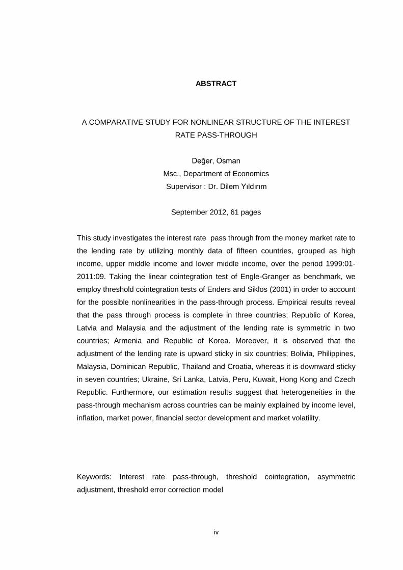
ABSTRACT

A COMPARATIVE STUDY FOR NONLINEAR STRUCTURE OF THE INTEREST

RATE PASS-THROUGH

Değer, Osman

Msc., Department of Economics

Supervisor : Dr. Dilem Yıldırım

September 2012, 61 pages

This study investigates the interest rate pass through from the money market rate to

the lending rate by utilizing monthly data of fifteen countries, grouped as high

income, upper middle income and lower middle income, over the period 1999:01-

2011:09. Taking the linear cointegration test of Engle-Granger as benchmark, we

employ threshold cointegration tests of Enders and Siklos (2001) in order to account

for the possible nonlinearities in the pass-through process. Empirical results reveal

that the pass through process is complete in three countries; Republic of Korea,

Latvia and Malaysia and the adjustment of the lending rate is symmetric in two

countries; Armenia and Republic of Korea. Moreover, it is observed that the

adjustment of the lending rate is upward sticky in six countries; Bolivia, Philippines,

Malaysia, Dominican Republic, Thailand and Croatia, whereas it is downward sticky

in seven countries; Ukraine, Sri Lanka, Latvia, Peru, Kuwait, Hong Kong and Czech

Republic. Furthermore, our estimation results suggest that heterogeneities in the

pass-through mechanism across countries can be mainly explained by income level,

inflation, market power, financial sector development and market volatility.

Keywords: Interest rate pass-through, threshold cointegration, asymmetric

adjustment, threshold error correction model

v

ÖZ

FAİZ ORANI YANSIMASININ DOĞRUSAL OLMAYAN YAPISININ

KARŞILAŞTIRMALI ÇALIŞMASI

Değer, Osman

Yüksek Lisans, İktisat Bölümü

Tez Yöneticisi: Dr. Dilem Yıldırım

Eylül, 2012, 61 Sayfa

Bu çalışma 01/1999 ve 09/2011 zaman aralığında, yüksek gelirli, orta gelirli ve

düşük gelirli olarak gruplandırılmış 15 ülkenin aylık verilerini kullanarak para

piyasası faiz oranının kredi faiz oranına yansımasını incelemektedir.Engle-

Granger’ın doğrusal eştümleşme sınamasını baz alarak yansıma mekanizmasındaki

olası doğrusalsızlıkları açıklayabilmek için Enders ve Siklos’un eşikli eştümleşme

sınaması uygulanmaktadır. Ampirik sonuçlar faiz yansıması sürecinin Güney Kore,

Letonya ve Malezya olmak üzere üç ülkede tamamlanmış olduğunu ve kredi faiz

oranı uyumunun Güney Kore ve Ermenistan olmak üzere iki ülke için bakışımlı

olduğunu göstermektedir.Buna ek olarak, Bolivya, Filipinler, Malezya, Dominik

Cumhuriyeti, Tayland ve Hırvatistan olmak üzere altı ülke için kredi faiz oranı

uyumunun yukarı yönlü yapışkan olduğu ve Ukrayna, Sri Lanka, Letonya, Peru,

Kuveyt, Hong Kong, Çek Cumhuriyeti olmak üzere 7 ülke için bu uyumun aşağı

yönlü yapışkan olduğu gözlenmektedir. Ayrıca, tahmin sonuçlarımız yansıma

mekanizmasının ülkeler arası heterojenliğinin temel olarak gelir düzeyi, enflasyon,

piyasa gücü, finans sektöründeki gelişmişlik ve piyasa oynaklığıyla

açıklanabileceğini göstermektedir.

Anahtar kelimeler: faiz yansıması, eşikli eştümleşme, bakışımsız uyum, eşikli hata

düzeltme modeli.

vi

To My Family

vii

ACKNOWLEDGMENTS

I am deeply indebted to my thesis supervisor Dr. Dilem Yıldırım for her stimulating

support and enlightening supervision throughout this study. I also tender my thanks

to examining committee members, Assoc. Prof. Dr. Işıl Erol and Assoc. Prof. Dr.

Tolga Omay.

I also thank my colleague from Middle East Technical University, Department of

Economics; research assistant Ceren Akbıyık for her valuable support and interest.

I would like to express my gratitude to my family for their understanding, assistance,

and for providing me with all the motivation and encouragement I need to fulfill this

study.

I also would like to express my very great appreciation to TUBİTAK for the financial

support I have received throughout my MSc. degree education.

viii

TABLE OF CONTENTS

PLAGIARISM ........................................................................................................... iii

ABSTRACT ............................................................................................................. iv

ÖZ ............................................................................................................................ v

DEDICATION .......................................................................................................... vi

ACKNOWLEDGMENTS ......................................................................................... vii

TABLE OF CONTENTS ......................................................................................... viii

LIST OF TABLES ..................................................................................................... x

LIST OF FIGURES ................................................................................................. xii

LIST OF ABBREVIATIONS ................................................................................... xiii

CHAPTER

1.INTRODUCTION .................................................................................................. 1

2. LITERATURE REVIEW ....................................................................................... 4

3. DATA ..................................................................................................................11

4. METHODOLOGY ...............................................................................................19

4.1 Linear Cointegration ......................................................................................19

4.2 Nonlinear Cointegration .................................................................................21

4.3 Nonlinear Threshold Error Correction Models ................................................24

5. EMPIRICAL RESULTS ......................................................................................26

5.1 Linear and Nonlinear Cointegration Test Results ..........................................26

5.1.1 Country Specific Results .........................................................................37

5.1.2 Results for Country Income Groups ........................................................43

5.2 Threshold ECM Results.................................................................................45

6. CONCLUSIONS .................................................................................................50

REFERENCES .......................................................................................................52

APPENDICES

A. Descriptive Statistics .......................................................................................58

ix

B. Macroeconomic and Financial Indicators ........................................................59

C. Tez Fotokopi İzin Formu .................................................................................61

x

LIST OF TABLES

TABLES

Table 1: Groups of Countries ..................................................................................11

Table 2: Ng and Perron (2001) Unit Root Test Results ...........................................18

Table 3: Estimated Long-run Equilibrium Relationships ..........................................27

Table 4: Cointegration Test Results for High Income Countries ..............................34

Table 5: Cointegration Test Results for Upper Middle Income Countries ................35

Table 6: Cointegration Test Results for Lower Middle Income Countries ................36

Table 7: Estimated Threshold Error-Correction Models for High Income Countries .47

Table 8: Estimated Threshold Error-Correction Models for Upper Middle Income ......

Countries ................................................................................................................48

Table 9: Estimated Threshold Error-Correction Models for Lower Middle Income ......

Countries ................................................................................................................49

Table 10:Correlation Coefficient between the Markup and the Money Market Rate ...

...............................................................................................................................58

Table 11:Macroeconomic and Financial Indicators .................................................59

https://sqrl.metu.edu.tr/src/THESIS.docx#_Toc334367158




xi

LIST OF FIGURES

FIGURES

Figure 1: Money Market Rate, Lending Rate and Markup Series of High Income

Countries over the Period 1999:01 to 2011:09 ........................................................13

Figure 2: Money Market Rate, Lending Rate and Markup Series of Upper Middle

Income Countries over the Period 1999:01 to 2011:09 ...........................................14

Figure 3: Money Market Rate, Lending Rate and Markup Series of Lower Middle

Income Countries over the Period 1999:01 to 2011:09 ...........................................15

Figure 4: Change in the Error-Correction Term Series of High Income Countries ...38

Figure 5: Change in the Error-Correction Term Series of Upper Middle Income

Countries ................................................................................................................39

Figure 6: Change in the Error-Correction Term Series of Lower Middle Income

Countries ................................................................................................................40












xii

LIST OF ABBREVIATIONS

AIC Akaike Information Criterion

CV Coefficient of Variation

ECM Error-Correction Model

ECT Error-Correction Term

EG Engle-Granger

GDP Gross Domestic Product

GNP Gross national Product

IPT Interest Rate Pass-Through

MTAR Momentum Threshold Autoregressive

TAR Threshold Autoregressive

1

CHAPTER 1

INTRODUCTION

Monetary policy is important for an economy in order to cope with the cyclical

downturns while attaining the price stability and promoting the economic growth.

This study analyses the dynamics of the monetary policy that is implemented

through the interest rate channel. Via this channel, most of the central banks use

their short term official rates to control the retail rates of banks which in turn enable

them to control the real side of the economy. Effectiveness of the monetary policy

depends on how fast and to what extend the retail rates respond to the changes in

the official rate.

The interest rate pass through (IPT) process includes two steps. In the first step,

central banks aim to alter the money market rate by changing the short term official

rates; and in the second step retail rates of banks change following changes in the

money market rate. The first step of the interest rate pass through is assumed to be

complete, so that changes in the official rate are fully transmitted to the money

market rate. As many studies1 show, the second step, however, may not be

complete and the speed of the pass through could change across countries.

According to the studies2, low level of competition among banks and asymmetric

information are the possible reasons behind an incomplete IPT. Moreover,

adjustment of retail rates to changes in the money market rate (or the official rate)

might differ across countries due to differences in level of income, inflation rate,

1 Cotterelli and Kourelis (1994), Mojon (2000), Sorensen and Werner (2006), Adams (2011),

Leuvensteijn (2011), Gigineishvili (2011), Hoffman (2006), Crespo-Cuaresma, Egert and Reininger (2006), Chinois and Leon (2005), de Bondt (2005), Liu, Margaritis and Tourani-Rad (2007), Hansen and Welz (2011), Friasancho-Mariscal and Howells (2011), Jobst and Kwapil (2008), Tai, Sek and Har (2012)

2 Sander and Kleimeier (2004a), Payne and Waters (2008), Wang and Lee (2009)

2

market uncertainty and the level of development of the financial sector. Furthermore,

an important number of studies3 show that retail rates adjust asymmetrically to

changes in the money market rate depending on different nonlinear drivers. Main

pillars of this asymmetry are given as switching, searching and menu costs, the

market power and moral hazard problems caused by imperfect information.

In this study, we aim to explore the pass through of the money market rate on the

lending rate4 over the sample period January 1999 – September 2011, in fifteen

countries which can be grouped according to the income levels as; high, upper

middle and lower middle. Various macroeconomic and financial indicators are

utilized to explain the heterogeneities in terms of the interest rate pass through

process across our sample countries. In order to reveal and compare the dynamics

of the pass through mechanism in our sample countries, we start with investigation

of the long-run relationship between the lending rate and the money market rate in

order to assess the completeness of the pass through process in these countries.

Next, taking the possibility of asymmetric adjustment of lending rates into account,

we perform the threshold autoregressive (TAR) and momentum threshold

autoregressive (MTAR) cointegration tests of Enders and Siklos (2001). Finally, we

employ threshold error correction models to uncover both short-run and long-run

dynamics of the interest rate pass through mechanism.

Our empirical findings show that the pass through mechanism is incomplete in

majority of our sample countries. Even though we expect to find a complete pass

through for high income countries, lending rates of majority of high income countries

exhibit incomplete pass through due to low level of competition in the banking

sector, high market volatility and relatively less developed financial market. For

3 Sholnick (1999), Crespo-Cuaresma, Egert, Reininger (2004), Mizen and Hofmann (2002),

Fuertes, Heffernan and Kalotychou (2009), Gambacorta and Iannotti (2005), Karagiannis, Panagopoulos and Vlamis (2010), Cecchin (2011), Liu, Margaritis and Tourani-Rad (2007), Amasekara (2005), Tkacz (2001), Payne and Waters (2008), Payne (2007a 2007b), Wang and Lee (2009), Thompson (2006), Sander and Kleimeier (2002, 2004a, 2004b), Hovarth (2004) and Sznajderska (2012).

4 The pass through from money market rate to deposit rate will be explored in a further

study.

3

almost all of our sample countries5 we observe substantial asymmetry in the

adjustment of lending rates. Moreover, the lending rate appears to be upward rigid

for Bolivia, Philippines, Malaysia, Dominican Republic, Thailand and Croatia, while

significant downward rigidity is observed for the lending rates of Sri Lanka, Ukraine,

Latvia, Peru, Kuwait, Hong Kong and Czech Republic. Heterogeneities in terms of

market volatility and market power seem to be possible reasons to observe different

form of asymmetries across countries. Furthermore, our nonlinear threshold error

correction model estimates suggest that the money market rate is weakly

exogenous in all countries, which constitutes the basis of our univariate modeling.

Contributions of this study are twofold. First, we explore the pass through

mechanism in seven countries6 which has not been studied so far. Second, we

reveal substantial differences in terms of completeness, speed of adjustment and

type of asymmetry in adjustment across countries by taking income level,

macroeconomic and financial indicators into account.

This study is organized as follows; Chapter 1 briefly introduces the study, Chapter 2

reviews the theoretical and empirical literature of the interest rate pass-through

mechanism, Chapter 3 presents the data with preliminary analysis, Chapter 4

describes the TAR and MTAR models, Chapter 5 discusses the empirical results

and finally Chapter 6 concludes the study.

5 The adjustment of the lending rate to changes in the money market rate is symmetric only

in Republic of Korea and Armenia.

6 Croatia, Kuwait, Dominican Republic, Peru, Ukraine, Armenia and Bolivia.

4

CHAPTER 2

1. LITERATURE REVIEW

Official short-term interest rates are one of the principal tools of implementing

monetary policy for many central banks. When the central bank changes its official

rate, it aims to affect first the money market rate, marginal cost of funds faced by

banks, and then the retail (loan and deposit) rates offered by banks to non-financial

institutions and households. Changes in retail rates will alter spending on durable

and investment goods along with the goals of monetary policy. Hence, effectiveness

of monetary policy depends on how complete and fast the pass-through to the

money market and retail rates is.

In the literature, the first step of the interest rate pass through (IPT) process is

generally assumed to be complete that is, changes in the official rate are fully

transmitted to the money market rate. With this assumption almost all existing

studies focus on the pass-through from the official rate or the money market rate to

retail rates.

Despite the importance of the speed, completeness and dynamics of the interest

rate pass through to observe the impact of the monetary policy on real side of

economy; earlier studies are more concentrated on the pass through of exchange

rates rather than interest rates. However, with the introduction of Euro and

especially after the 2008-2009 world financial crisis, the way retail rates respond to

money market and/or official rate changes has become a growing concern of

researchers. Consequently, literature on the interest rate pass through (IPT) to retail

rates has grown in the last decades.

Depending on financial and money market conditions, retail rates may adjust slowly

to money market rate (official rate) changes, suggesting a sticky structure, which in

5

turn may breed an incomplete pass through. For example, in low income countries

with low level of gross domestic product (GDP) and an undeveloped financial sector,

banks may adjust their retail rates slowly due to being in a less competitive

environment, where the variety of banks’ products is limited and consumers are not

informed well about the market and choices they have. As suggested by the

standard Cournot model in microeconomics, those banks will have more power over

the market and be more profitable, which may result in a sluggish adjustment. In

high income countries, on the other hand, due to developed financial sector and

high competition among banks, which implies a low bank concentration ratio (a

competitiveness measure), we would expect a faster adjustment in retail rates.

There is no doubt that the IPT process will be affected by consumers’ behaviors as

well. High demand for loans or other products will lead to higher number of suppliers

which in turn decreases the bank concentration ratio, increases competitiveness of

the market along with the adjustment of retail rates. Regarding money market

conditions, the inflation rate and market uncertainty could be quite effective on the

IPT. In a high inflationary environment, banks should update their rates (especially

the lending rate, in order to make sure that the real interest rate is positive) more

frequently, speeding up the pass through. Higher volatility of the money market rate

or the official rate, on the other hand, may slow down the adjustment, since banks

will hesitate to make changes.

Being in line with the discussion above, Cotterelli and Kourelis (1994), reveal that

less barriers to competition speed up the pass through mechanism. Similarly, Mojon

(2000), Sorensen and Werner (2006), Adams (2011), Leuvensteijn (2011) and

Gigineishvili (2011) show that bank concentration (competition) lowers (increases)

the adjustment speed of retail rates following changes in the money market rate (or

the official rate). Gigineishvili (2011) reveals further that the IPT is faster for

countries with higher per capita GDP. Regarding effect of monetary conditions,

Cotterelli and Kourelis (1994) and Gigineishvili (2011) provide empirical support for

the positive impact of inflation on speed of adjustment, while Giginieishvili (2011),

Cotterelli and Kourelis (1994), Mojon (2000) and Sander and Kleimeier (2004b)

point out that the higher the market volatility, the lower the speed of the IPT process

is.

6

Beside these, there are also studies aim to explore whether there is a structural

break effect on the speed and completeness of the IPT. In this sense, Hofmann

(2006), Egert, Crespo-Cuaresma, and Reininger (2007), Chionis and Leon (2005)

and de Bondt (2005) examine the effect of introduction of the single currency, Euro,

on the pass through of interest rates. Analyzing different types of retail rates through

error correction models, they find out that the speed of pass through has increased

with the introduction of the euro for all EU members, except Germany. Similarly, Liu,

Margaritis and Tourani-Rad (2007), uncovers that introduction of official cash rate7

in New Zeland has increased the speed of pass through. Hansen and Welz (2011),

Friasancho-Mariscal and Howells (2011) and Jobst and Kwapil (2008) investigate

the effect of 2008 crisis on the speed of pass through. The overall conclusion is

crisis has weakened the interest rate pass through in Sweden, Austria, US and EU

as well as UK if deposit rates are considered. Tai, Sek and Har (2012) obtain

similar results for Asian countries after the Asian crisis.

The literature discussed above presumably assumes symmetric adjustment of

interest rates to money market rate changes. However, generally, it is not the case.

Besides financial and money market conditions discussed above, there are various

reasons to expect an asymmetric pass-through. Existence of switching costs8 and

searching costs9 are some of the reasons to observe asymmetries in adjustment.

Existence of these costs increase the market power of banks, Lowe and Rohling

(1992), and enable banks to increase (decrease) their lending rates faster (slower)

when the money market rate rises (falls), Scholnick (1999). Secondly, asymmetric

pass-through of lending rates may arise from the imperfect information problem.

According to Striglitz and Weiss (1981), for banks, riskiness of the loan is as

important as the interest revenue collected. Since the demand for loans would be

less elastic for risky borrowers, an increase in the lending rate will attract more risky

borrowers compared to credible ones. In order to overcome the moral hazard

7 A policy –controlled benchmark interest rate, on money market and residential lending

rates in New Zeland. Liu et Al. (2007)

8 The costs incurred when customers change their banks or change the type of loan they are

using.

9For banks,e.g. cost of gathering information about the customer; for customers, e.g. cost of

learning the rates offered and the payment schedule by each individual bank,

7

problem, banks may act slowly following an increase in the money market rate.

Moreover, Hannan and Berger (1991), Neumark and Sharpe (1992) and Scholnick

(1996) argue that asymmetric adjustment may stem from collusive pricing

arrangements and adverse customer reaction. Collusive pricing arrangement theory

suggests that it is unprofitable for a bank to act against collusive pricing behaviour.

In cases of both increasing and decreasing the lending rate the bank faces costs.

Yet, additional cost generated by decreasing the lending rate is greater than the cost

while increasing it.Therefore, lending rates should be downward sticky.On the other

hand, adverse customer reaction theory suggests that when a bank acts against the

collusive pricing and alters the lending rate, customers may react negatively to the

change. If additional costs generated by altering the lending rate depend heavily on

negative reaction of the cumstomers, the bank will act more slowly to increase its

lending rate. Thirdly, menu costs10 (adjustment costs) might lead banks to act slowly

when changes in money market rate are relatively small, but respond faster

following large changes in the money market rate. Finally, as Dueker (2000)

suggests, asymmetric pass-through is expected due to business cycles. He asserts

that banks are risk averse so that they act slowly to lower their lending rates during

cyclical downturns, suggesting that the expansionary monetary policy will be less

effective on the economy compared to the contractionary monetary policy.

Due to the reasons discussed above, recent literature is mainly focused on

asymmetric structure of the IPT in order to explore the dynamics of the adjustment

process more precisely. Empirical studies investigating asymmetries in the interest

rate pass-through employ generally nonlinear threshold error-correction models

(ECMs), where the long run equilibrium is represented in terms of cointegration

between official rate or the money market rate and the retail loan rate. Within this

framework, the pass-through is examined for a number of countries in studies:

Mizen and Hofmann (2002) and Fuertes, Heffernan and Kalotychou (2009) for UK,

Tkacz (2001), Scholnick (1999), Karagiannis, Panagopoulos and Vlamis (2010),

Thompson (2006), Wang and Lee (2009), Payne and Waters (2008), and Payne

(2006,2007) for US, Karagiannis et al. (2010) and Sander and Kleimeier

(2002,2004) for EU countries, Scholnick (1999) for Canada, Crespo-Cuaresma,

10

The cost of changing the initial lending rate such as cost of advertising or announcement, labor time devoted to apply changes.

8

Egert, Reininger (2004), for Czech Republic, Hungary and Poland, Gambacorta and

Iannotti (2005), for Italy, Amasekara (2005), for Sri Lanka, Cecchin(2011), for

Switzerland, Horvarth (2004), for Hungary, Sznajderska (2012), for Poland, Liu et

Al. (2007) for New Zealand and Wang and Lee(2009) for Asian countries.

The studies allowing for asymmetry in the IPT process can be separated into two in

terms of determination of the threshold value. While some of the studies determine

the threshold value exogenously, others treat the threshold as an unknown

parameter and estimate it by an appropriate methodology. In this sense, Scholnick

(1999), Crespo-Cuaresma et al. (2004), Mizen and Hofmann (2002) and Fuertes et

Al. (2009), Gambacorta and Iannotti (2005), Karagiannis et al. (2010), Cecchin

(2011) and Liu et al. (2007) set exogenous threshold values, while Tkacz (2001),

Payne and Waters (2008), Payne (2006, 2007), Wang and Lee (2009), Thompson

(2006), Sander and Kleimeier (2002, 2004a), Hovarth (2004) and Sznajderska

(2012) utilize methods allowing for an endogenously determined threshold value.

The first group of studies on asymmetric IPT set threshold value to zero in order to

observe asymmetries driven by negative/positive deviations from the equilibrium.

However the threshold is not necessarily zero, it may change according to the

structure of the data. In this sense, finding a consistent estimator for the unknown

threshold value is important to explore the IPT process more precisely. All of the

studies11 in the second group except for Tkacz (2001) employ Threshold

Autoregressive (TAR) and Momentum Threshold Autoregressive (MTAR) models

proposed by Enders and Siklos (2001) to test for asymmetry and cointegration while

estimating the unknown threshold value through the methodology of Chan (1993).

Empirical studies on the asymmetric pass through of American interest rates with an

endogenously determined threshold value reach to opposing conclusions. While

Tkacz (2001) fail to detect an asymmetry in the adjustment of the prime rate to

changes in the Federal Funds rate, Payne and Waters (2008) and Payne (2007)

reveal significant asymmetries in the adjustment of prime rate and adjustable rate

11

Tkacz (2001) estimates threshold using Hansen’s grid search method.

9

mortgages: on newly built homes and previously owned homes, respectively, with

the rates reacting slower (faster) when there is an increase (decrease) in the

Federal Funds rate. Analyzing the spread between the prime rate and the deposit

rate, Thompson (2006) points out that the spread is more sluggish when it is above

its threshold value.

Sander and Kleimeier (2002, 2004) employ both exogenously and endogenously

determined threshold values to explore the asymmetric nature of the IPT in fifteen

EU countries. According to their findings, majority of EU countries have asymmetry

in the IPT. They argue further that the introduction of euro has not changed the

heterogeneous nature of the IPT across Euro area. In other words, changes in

money market rates result in different pass through nature in the area even after the

introduction of euro.

In terms of asymmetric adjustment of interest rates in other countries; Wang and

Lee (2009) uncover that, lending rates adjust asymmetrically in Philippines, Taiwan,

and Hong Kong, exhibiting downward stickiness. In Poland, relatively longer term

credits show downward rigidity whereas short term loans such as credit rates to

consumers exhibit upward rigidity. Hovarth (2004) and Sznajderska (2012) also

reveal that larger shocks are eliminated rather quickly in Hungary and Poland,

respectively.

This study aims to explore the pass through from the money market rate to the retail

loan rates in 15 different countries. Similar to the most recent studies we aim to

reveal asymmetries, nonlinearites,in the responses of loan rates through univariate

threshold autoregressive (TAR) and momentum threshold autoregressive (MTAR)

models of Enders and Siklos (2001). Our study, however, differs from the existing

ones in that we account not only for asymmetries but also income differences across

countries. In that sense, we group Croatia, Czech Republic, Hong Kong, Kuwait and

Republic of Korea as high income, Latvia, Malaysia, Dominican Republic, Peru and

Thailand as upper middle income and Ukraine, Armenia, Sri Lanka, Philippines and

Bolivia as lower middle income countries. Among our sample countries, the pass

10

through from money market rate (or the official rate) to lending rates is studied for

the countries Hong Kong, Republic of Korea, Malaysia, Philippines and Thailand

Wang and Lee (2009), Sri Lanka by Amasekara (2005), Czech Republic by Crespo-

Cuaresma et al. (2004) and Sander and Kleimeier (2004b), and Latvia by Sander

and Kleimeier (2004b). Investigation of the IPT for the rest of the countries in our

sample; Croatia, Kuwait, Dominican Republic, Peru, Ukraine, Armenia and Bolivia

will be first in literature.

11

HIGH INCOME UPPER MIDDLE INCOME LOWER MIDDLE INCOME

Kuwait Latvia Ukraine

Hong Kong Malaysia Armenia

Republic of Korea Dominican Republic Sri Lanka

Czech Republic Peru Philippines

Croatia Thailand Bolivia

CHAPTER 3

5. DATA

This study utilizes monthly data of fifteen countries – (Kuwait, Hong Kong, Republic

of Korea, Czech Republic, Croatia, Latvia, Malaysia, Dominican Republic, Peru,

Thailand, Ukraine, Armenia, Sri Lanka, Philippines, Ukraine) to analyze the interest

rate pass through process from the money market rate to the lending rate. For each

country; money market and lending rate monthly series covering the period of

January 1999 to September 2011 are obtained from International Financial Statistics

(IFS) database. The starting date of 1999 is selected in order to avoid the effects of

the Asian crisis in 1997 and 1998, which results in extraordinary behaviors in

interest rates.

Countries in interest are grouped according to country classification method of the

World Bank. High income group refers to the countries with gross national income

(GNI) per capita of $12.476 or more. Countries that have GNI per capita between

$4,036 and $12,475 fall into the upper middle income group and finally lower middle

income group covers the countries with GNI per capita between $1,026 and

$4,03512. Table 1 summarizes the countries according to their income levels.

Table 1: Groups of Countries

12

Countries are grouped according to their 2011 GNI per capita levels.

12

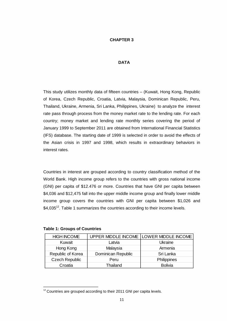
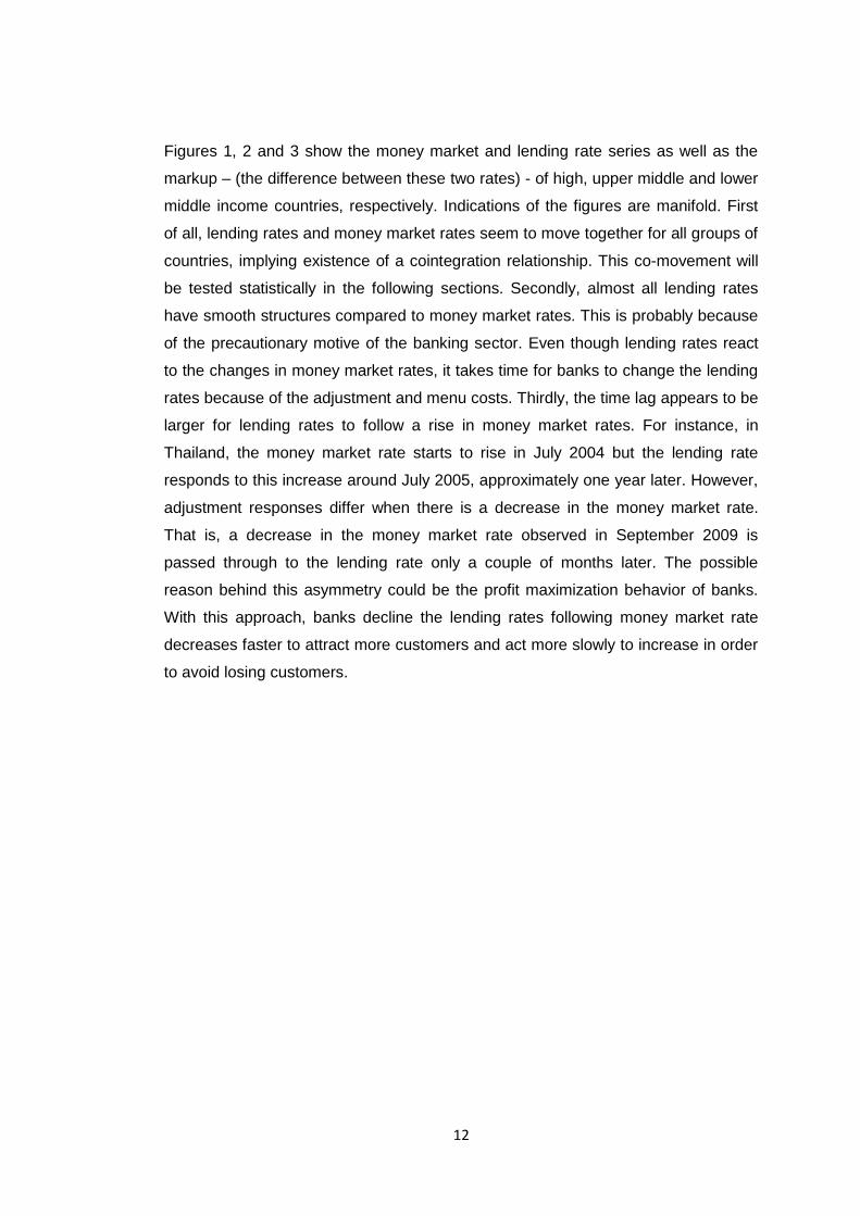
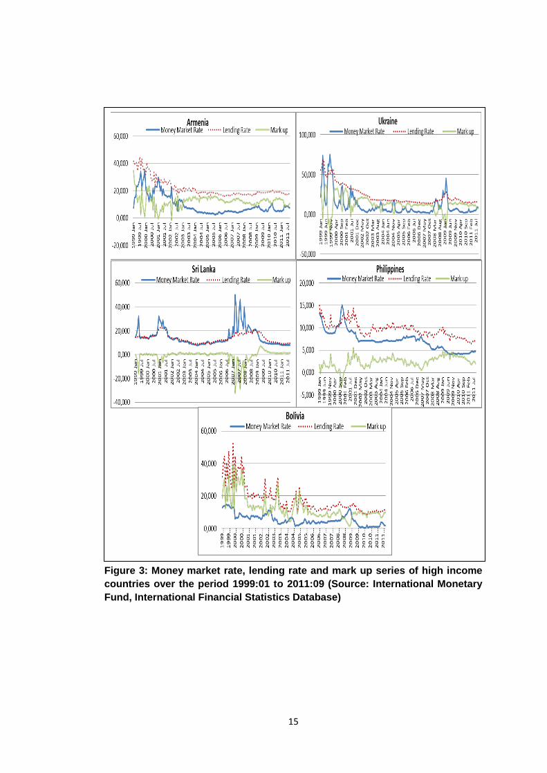
Figures 1, 2 and 3 show the money market and lending rate series as well as the

markup – (the difference between these two rates) - of high, upper middle and lower

middle income countries, respectively. Indications of the figures are manifold. First

of all, lending rates and money market rates seem to move together for all groups of

countries, implying existence of a cointegration relationship. This co-movement will

be tested statistically in the following sections. Secondly, almost all lending rates

have smooth structures compared to money market rates. This is probably because

of the precautionary motive of the banking sector. Even though lending rates react

to the changes in money market rates, it takes time for banks to change the lending

rates because of the adjustment and menu costs. Thirdly, the time lag appears to be

larger for lending rates to follow a rise in money market rates. For instance, in

Thailand, the money market rate starts to rise in July 2004 but the lending rate

responds to this increase around July 2005, approximately one year later. However,

adjustment responses differ when there is a decrease in the money market rate.

That is, a decrease in the money market rate observed in September 2009 is

passed through to the lending rate only a couple of months later. The possible

reason behind this asymmetry could be the profit maximization behavior of banks.

With this approach, banks decline the lending rates following money market rate

decreases faster to attract more customers and act more slowly to increase in order

to avoid losing customers.

13

FIGURE 1: Money market rate, lending rate and markup series of high income

countries over the period 1999:01 to 2011:09. (Source: International Monetary

Fund, International Financial Statistics Database)

14

-

Figure 2: Money market rate, lending rate and markup series of upper middle income countries over the period 1999:01 to 2011:09. (Source: International Monetary Fund, International Financial Statistics Database)

15

Figure 3: Money market rate, lending rate and mark up series of high income

countries over the period 1999:01 to 2011:09 (Source: International Monetary

Fund, International Financial Statistics Database)

16

Moreover, as seen in Figures 1-3, the spread (markup) between two rates is smaller

for high income economies, generally lower than five percent. For the upper middle

income group, on the other hand, the markup gets as high as almost thirty percent,

and for lower middle income countries, a markup that is around forty percent is

experienced. Inflation could be the main cause of such differences among income

groups. As expected, the inflation rate in lower middle income countries is much

higher than the one in upper middle and high income groups. The annual average

inflation rate over the period from 1999 to 2011 is between 0.2% and 3.5% for high

income countries, %2.3 and %11.7 for upper middle income group, %4 and %13.2

for lower middle income group13. Moreover, as may be expected, the markup

becomes negative during crisis which occurs more frequently in lower middle

income group countries14.

Finally, the negative relationship between money market rates and the markups can

be easily seen from the figures. Simply, when the money market increases

(decreases) while the lending rate stays relatively same, we will observe a decline

(rise) in markup, resulting in a negative correlation between the money market rate

and the markup. Given this, it can be concluded that the slower the adjustment of

lending rates the stronger the negative relationship would be. As an example, the

coefficient of correlation between the money market rate and the markup is -0.029 in

Latvia, indicating very weak negative linear relationship and hence, raising the

possibility of complete pass-through. For Philippines, on the other hand, a relatively

13

Sri Lanka is the only country that does not suit to this relation. It has one of the highest inflation rates (9.61%) within our sample countries with a markup very close to zero. However, this surprising relation originates from the fact that most of the large banks in Sri Lanka are state-owned. In order to promote economic growth, state banks do not add noticeable markup to their marginal costs-(money market rate).

14 A negative markup denotes that banking sector is open to outside shocks and there is a

coordination problem between policy makers and banks. During crisis, money market rates increase sharply and unexpectedly. As it takes time for banks to adjust their rates, they have lower lending rate (or price) than the money market rate (or the marginal cost) during the shocks, signaling that banking sector is making losses raising the risk of bankruptcy. Lower middle income countries face this problem more frequently, related to their underdeveloped financial system and openness to shocks.

17

high correlation coefficient of -0.668 is observed and this may suggest an

incomplete IPT process15.

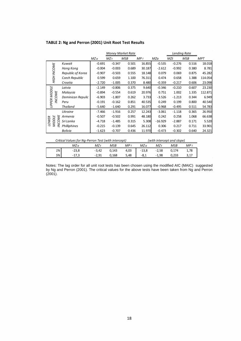
As a preliminary analysis, we prefer to employ Ng and Perron (2001)16 unit root

tests, since they are modified versions of the existing unit root tests with better

performance in terms of power and size distortions. Unit root test results together

with the corresponding critical values are represented in Table 2. As is frequently

the case for interest rates, a conventional unit root analysis does not reject the null

hypothesis of a unit root in each interest rate series for all countries at the 5 percent

level. Although macroeconomic arguments may point to the stationarity of interest

rates, our data have statistical properties associated with nonstationary, or near-

nonstationary, I(1) series. Consequently, and following earlier studies, we proceed

to a cointegration analysis of the pass-through.

15

See Appedix-A for correlation coefficients of all countries.

16 Ng and Perron (2001) constructed four different unit root test statistics that are estimated

using generalized least squares (GLS) de-trended data for each variable. These test statistics are modified forms of Phillips and Perron statistic, the Bhargava (1986) statistic and Elliot, Rothenberg and Stock (ERS) point optimal statistic. Traditional unit root tests typically suffer from severe finite sample power and size problems, whereas Ng-Perron test corrects for size distortions and has good power in finite sample.

18

TABLE 2: Ng and Perron (2001) Unit Root Test Results

Notes: The lag order for all unit root tests has been chosen using the modified AIC (MAIC) suggested by Ng and Perron (2001). The critical values for the above tests have been taken from Ng and Perron (2001).

MZ a MZ t MSB MP T MZa MZt MSB MPT

Kuwait -0.691 -0.347 0.501 16.855 -0.535 -0.276 0.516 18.018

Hong Kong -0.004 -0.003 0.689 30.187 -2.612 -0.992 0.380 8.781

Republic of Korea -0.907 -0.503 0.555 18.148 0.079 0.069 0.875 45.282

Czech Republic 0.599 0.659 1.100 76.311 0.474 0.658 1.388 114.054

Croatia -2.720 -1.005 0.370 8.480 -0.359 -0.217 0.606 23.098

Latvia -2.149 -0.806 0.375 9.640 -0.346 -0.210 0.607 23.230

Malaysia -0.894 -0.554 0.619 20.976 0.751 1.002 1.335 112.871

Dominican Repulic -6.903 -1.807 0.262 3.733 -3.526 -1.213 0.344 6.949

Peru -0.191 -0.162 0.851 40.535 0.249 0.199 0.800 40.540

Thailand -5.640 -1.640 0.291 16.077 -0.968 -0.495 0.511 54.783

Ukraine -7.466 -1.916 0.257 12.243 -3.061 -1.118 0.365 26.950

Armenia -0.507 -0.502 0.991 48.180 0.242 0.258 1.068 66.638

Sri Lanka -4.718 -1.485 0.315 5.308 -16.929 -2.887 0.171 5.520

Philliphines -0.215 -0.139 0.645 26.112 0.306 0.217 0.711 33.901

Bolivia -1.623 -0.707 0.436 11.970 -0.473 -0.302 0.640 24.321

MZ a MZ t MSB MP T MZ a MZ t MSB MP T

1% -23,8 -3,42 0,143 4,03 -13,8 -2,58 0,174 1,78

5% -17,3 -2,91 0,168 5,48 -8,1 -1,98 0,233 3,17

Critical Values for Ng-Perron Test (with intercept) (with intercept and slope)

Money Market Rate Lending RateH

IGH

INC

OM

EU

PP

ER M

IDD

LE

INC

OM

E

LOW

ER

MID

DLE

INC

OM

E

19

CHAPTER 4

5. METHODOLOGY

In this study, we investigate the interest rate pass through from money market rates,

proxy for official rates, to retail lending rates. Under the assumption of weak

exogeneity of money market rates to lending rates, we utilize a single equation

modeling approach to reveal short run and long run dynamics of the pass through

mechanism.

4.1 Linear Cointegration

Given the I(1) structures of the interest rates along with the co-movement of lending

rates ( lr ) and money market rates ( mmr ) observed from Figures 1-3, our starting

point for formulizing the pass through process is the linear cointegration test. In this

sense, we utilize the Engle and Granger (1987) cointegration test to figure out the

relationship between lending rate and money market rate and estimate the following

long run equilibrium regression by the Ordinary Least Squares (OLS) method:

t t tlr mmr u

where tmmr and tlr refer to the money market and lending rates, respectively, and

tu is the stochastic disturbance term measuring the deviation of the lending rate

from its equilibrium path. In this regression, captures the mark-up between mmr

and lr , while , the degree of pass through, measures the magnitude of the

change in mmr that is passed on to lr in the long run. The pass through is complete

(1)

20

if 1 , since under this circumstance, any change in the mmr is fully transmitted to

the lr . On the other hand, if 1 the pass through is incomplete, in the sense

that, even in the long run, changes in mmr are reflected partially on lr .

Completeness of the pass through mechanism is an indicator of the effectiveness of

monetary policy, for this reason, the null hypothesis of complete pass through:

0 : 1H , is statistically tested17.

Once the residuals, ˆtu , are obtained from the regression (1), the second step of

Engle-Granger testing methodology involves testing for cointegration, stationarity of

ˆtu through the regression:

1

1

ˆ ˆ ˆp

t t i t p t

i

u u u

17

Although in equation (1) exhibits the degree of pass through, Benarjee, Dolado, Hendry

and Smith (1986) indicate that the estimator of the degree of pass through may suffer from biasedness and underestimation problems. To overcome this problem, Bardsen (1989) suggests the following ARDL model:

1 1* * * *

0

1 0

p q

t i t i i t i p t p q t q t

i i

lr lr mmr lr mmr

where p and q are the optimal lag lengths observed by Akaike’s Information Criterion with

the upper limit of

0.25

100, int 12 Tp q

where T is the sample size.

The unbiased estimator of the coefficient that measures the degree of pass through is

ˆˆ

ˆ

q

p

with the corresponding standard error being;

22

* * * * *ˆ ˆ ˆ ˆ ˆˆ ˆ ˆ ˆ ˆ ˆ( ) var( ) var( ) 2 cov( , )p q p p qse

Finally, testing for a complete pass-through turns to testing the null hypothesis of

0 : 1H

(2)

21

where, t is identically and independently distributed (iid) disturbance term and p is

the lag order that ensures the iid structure of t . Then, simply rejecting the null

hypothesis of 0 implies stationarity of ˆtu , namely existence of a long-run

equilibrium between the money market and lending rate.

4.2 Nonlinear Cointegration

As discussed in Chapter 2, there are many reasons to expect an asymmetric

structure in the interest rate pass through. In the presence of asymmetry,

nonlinearity, the linear cointegration test proposed by Engle and Granger (1987)

may be misleading, since it assumes symmetric adjustment to the equilibrium.

Enders and Siklos (2001) address to this misspecification problem and suggest

nonlinear cointegration tests allowing for a threshold autoregressive (TAR) and

momentum threshold autoregressive (MTAR) type adjustments.

In order to test for TAR type cointegration, similar to Engle-Granger methodology,

we first obtain residuals from equation (1), and then estimate the following

secondary regression:

1 1 2 1

1

ˆ ˆ ˆ ˆ1p

t t t t t i t p t

i

u I u I u u

where t is the iid disturbance term, ensured by the lag order p and tI is the

Heaviside Indicator function such that:

1

1

ˆ1

ˆ0

t

t

t

uifI

uif

(3)

(4)

22

where, is the unknown threshold value, such that if the previous period’s residual ,

1ˆ

tu , is above this threshold, the speed of adjustment is measured by 1 and if it is

below the threshold, 2 is the coefficient for speed of adjustment. It is easy to see

that when 1 2 , the TAR model turns to the standard Engle- Granger model.

Hence, Engle-Granger cointegration test which assumes symmetric adjustment is a

special case of the TAR model.

In order to obtain a consistent estimator for the unknown threshold value, , we

follow the procedure proposed by Chan (1993). In this context, we start with ranking

the residuals obtained from equation (1) in ascending order. Then, for each potential

threshold value , which is typically in the middle 70% of the ordered values of the

residuals, we estimate the TAR model (3) by OLS. Finally, the consistent estimator

of the threshold value is determined by minimizing the sum of squared residuals

over these estimations.

Once the threshold value is observed, the TAR model is estimated by OLS and the

existence of the cointegration between the lending rate and money market rate is

tested by the null hypothesis of: 0 1 2: 0H . The test statistic is symbolized as

and does not follow a standard F distribution, due to the threshold value being

unidentified under the null hypothesis of no cointegration (the well-known Davies

(1987) problem). To address this issue, Enders and Siklos (2001) perform a Monte

Carlo simulation in order to obtain the relevant critical values.

When significance of the cointegration is achieved and necessary and sufficient

conditions18 for the stationary of ˆ

tuholds, the next step is testing for significance of

asymmetry. As such, the null hypothesis of 1 2 is tested by a standard F test.

Chan and Tong (1989) show that; if consistency of the estimated threshold value is

18

According to the study of Petrucelli and Woolford (1984), 1 and 2 should be negative

and 1 2(1 )(1 ) 1 for any threshold value.

23

established, the asymptotic normality of the coefficients will hold, which in turn

allows us to employ standard F test.

The steps of testing for MTAR type asymmetric cointegration are not far different

from the TAR model. The main difference between these two models is simply the

type of asymmetry that is considered. The TAR model assumes that the adjustment

rate of residuals, 1 and 2 , differ depending on whether one lagged value of

residuals is above or below the threshold value. Hence, if the threshold value takes

a value close to zero, asymmetry with regard to the sign of the disequilibrium is

expected. However, the MTAR model considers the asymmetry that may be caused

by the change in the 1ˆ

tu rather than its level form.

In order to utilize the MTAR model, we start with estimation of the equation (1) and

obtain residuals. Then, employing the residuals, equation.(3) is estimated with the

following indicator function:.

1

1

ˆ1

ˆ0

t

t

t

uifI

uif

where, is the unknown threshold value estimated following the methodology of

Chan (1993), as in TAR type asymmetry. 1 ( 2 ) is the adjustment coefficient if

previous period’s change in residuals is relatively large (small), in other words,

change in 1ˆ

tu is greater than or equal to (less than) the threshold value.

(5)

24

4.3 Nonlinear Threshold Error Correction Model

When a non-linear cointegration relationship is achieved, the next step should be

constructing an appropriate threshold error-correction model to reveal both short run

and long run dynamics of the interest rate pass through simultaneously. The

asymmetric error correction model (ECM) has the form:

0 1 1 2 1 1

1 1

ˆ ˆ(1 )p p

t i t i i t i t t t t t

i i

lr lr mmr I u I u

where p is required number of lagged variables of lending rate and money market

rate that ensures the i.i.d. structure of the error term 1t , 1 1 1t t tu lr mmr

and the indicator function tI takes the form given in (4) and (5) for TAR-ECM and

MTAR-ECM, respectively. 1 ( 2 ) is the error correction term or the speed of

adjustment of lending rates to the long-run equilibrium in when is 1ˆtu ( 1

ˆtu )

for the TAR model and 1ˆtu ( 1

ˆtu ) for the MTAR model. i and i are the

coefficients of the lagged values of change in the lending rate and the money market

rate, respectively. Significance of i represents that changes in lending rate

depends on not only the changes in the money market rate but also its own past. i

, on the other hand, shows whether the previous periods’ changes in the money

market rate shapes this period’s change in the lending rate. Consequently rejection

of the null hypothesis of 0 1: ... 0pH indicates that money market rate

Granger causes the lending rate in the short run.

Similar to many existing studies in the interest rate pass-through literature, we

assume that the lending rate is affected by money market rate changes while the

money market rate is weakly exogenous to the lending rate. Even though it is

important to examine the exogeneity in order to investigate the pass-through

(6)

25

mechanism in a more comprehensive manner, very few studies19 perform weak

exogeneity of the money market rate and granger-causality tests. To test for the

validity of weak exogenity assumption we re-construct the nonlinear ECM with the

dependent variable being the money market rate as follows:

0 1 1 2 1 2

1 1

ˆ ˆ(1 )p p

t i t i i t i t t t t t

i i

mmr lr mmr I u I u

This form of ECM allow us to explore the weak exogeneity of the money market rate

making use of the error correction terms 1 and 2 ,such that if both error correction

terms are statistically insignificant, weak exogeneity assumption will be supported.

i and i are the coefficients of the lagged values of change in the lending rate and

the money market rate, as before. Significance of i represents that changes in the

money market rate depends on previous periods’ changes in the lending rate.

Failure of rejection of the null hypothesis: 0 1: ... 0pH suggests that the

money market rate is not Granger caused by the lending rate. However, as Engle,

Hendry and Richard (1983) underlines, changes in the money market rate may be

affected by changes in the lending rate, in other words the money market rate may

be Granger caused by the lending rate in the short-run, but this does not violate the

weak exogeneity of the money market rate. On the other hand, i are the

coefficients on the previous periods’ changes in the money market rate, hence

rejecting the null hypothesis 0 1: ... 0pH shows that a change in the money

market rate does not have impacts on changes in latter periods.

19

Payne(2007), Enders and Siklos (2001), Amasekara (2005)

(7)

26

CHAPTER 5

.EMPRICAL RESULTS

As mentioned before, our aim is to explore the pass through of the money market

rate on the lending rate over the sample period January 1999 – September 2011, in

fifteen countries which can be grouped according to their income levels as; high,

upper middle and lower middle making use of financial and macroeconomic

indicators. As such, after discussing the long-run relationship between the lending

rate and the money market rate for these countries through linear and nonlinear

cointegration tests (section 5.1), the estimated threshold ECMs are provided in

section 5.2.

5.1 Linear and Nonlinear Cointegration Test Results

Given the nonstationary structures of the interest rates, we first employ the standard

Engle-Granger cointegration approach in order to test for cointegration between the

lending rates and the money market rates. As such, we first estimate the long run

equilibrium equation given in (1). Before proceeding with the Engle-Granger

cointegration test results, we discuss the estimates of (1) in order to gain some

inference regarding the mark-up (down) and the degree (extend) of the pass-

through. Table 3 represents the estimation results of (1) for all countries. Regarding

the mark-up pricing policy, overall we observe that the mark-up values increase as

the income level decreases so that lowest mark-up values are observed in high

income countries. Moreover, it is seen that countries with high (low) markups

27

Table 3: Estimated Long-run Equilibrium Relationships

Notes: α and β are estimated parameters of (1) with standard errors given in parentheses.

4.845 0.633

(0.118) (0.029)

4.668 0.689

(0.063) (0.020)

3.161 0.897

(0.250) (0.061)

4.839 0.474

(0.068) (0.019)

10.165 0.227

(0.201) (0.036)

6.676 0.957

(0.478) (0.121)

3.806 0.885

(0.397) (0.135)

13.903 0.588

(0.579) (0.034)

19.677 0.774

(0.373) (0.052)

6.062 0.325

(0.170) (0.068)

16.093 0.664

(0.825) (0.046)

14.677 0.741

(0.555) (0.046)

8.338 0.369

(0.432) (0.026)

5.213 0.611

(0.265) (0.035)

8.536 1.716

-1.005 (0.155)

Philippiness No

Bolivia No

Armenia No

Sri Lanka No

Thailand No

LOWER MIDDLE INCOME

Ukraine No

Dominician Republic No

Peru No

UPPER MIDDLE INCOME

Latvia Yes

Malaysia Yes

Czech Republic No

Croatia No

Hong Kong No

Republic of Korea Yes

HIGH INCOME

Kuwait No

1

28

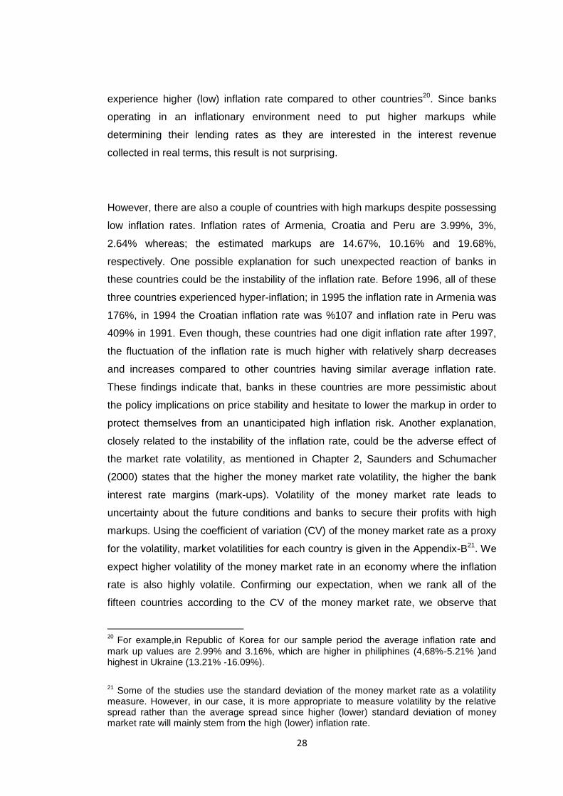
experience higher (low) inflation rate compared to other countries20. Since banks

operating in an inflationary environment need to put higher markups while

determining their lending rates as they are interested in the interest revenue

collected in real terms, this result is not surprising.

However, there are also a couple of countries with high markups despite possessing

low inflation rates. Inflation rates of Armenia, Croatia and Peru are 3.99%, 3%,

2.64% whereas; the estimated markups are 14.67%, 10.16% and 19.68%,

respectively. One possible explanation for such unexpected reaction of banks in

these countries could be the instability of the inflation rate. Before 1996, all of these

three countries experienced hyper-inflation; in 1995 the inflation rate in Armenia was

176%, in 1994 the Croatian inflation rate was %107 and inflation rate in Peru was

409% in 1991. Even though, these countries had one digit inflation rate after 1997,

the fluctuation of the inflation rate is much higher with relatively sharp decreases

and increases compared to other countries having similar average inflation rate.

These findings indicate that, banks in these countries are more pessimistic about

the policy implications on price stability and hesitate to lower the markup in order to

protect themselves from an unanticipated high inflation risk. Another explanation,

closely related to the instability of the inflation rate, could be the adverse effect of

the market rate volatility, as mentioned in Chapter 2, Saunders and Schumacher

(2000) states that the higher the money market rate volatility, the higher the bank

interest rate margins (mark-ups). Volatility of the money market rate leads to

uncertainty about the future conditions and banks to secure their profits with high

markups. Using the coefficient of variation (CV) of the money market rate as a proxy

for the volatility, market volatilities for each country is given in the Appendix-B21. We

expect higher volatility of the money market rate in an economy where the inflation

rate is also highly volatile. Confirming our expectation, when we rank all of the

fifteen countries according to the CV of the money market rate, we observe that

20

For example,in Republic of Korea for our sample period the average inflation rate and

mark up values are 2.99% and 3.16%, which are higher in philiphines (4,68%-5.21% )and highest in Ukraine (13.21% -16.09%).

21 Some of the studies use the standard deviation of the money market rate as a volatility

measure. However, in our case, it is more appropriate to measure volatility by the relative spread rather than the average spread since higher (lower) standard deviation of money market rate will mainly stem from the high (lower) inflation rate.

29

Armenia, Croatia and Peru listed among the highest volatile group. Market structure

might also explain the reason of high markups observed in these three countries.

According to Monti-Klein22 model, for markets that are far from perfect competition,

the demand for goods (bank products) will be less elastic which will in turn result in

higher markups. In other words, it is easy and profitable for banks to set high

markups in the absence of competition. Following the literature, we measure the

degree of competition by the bank concentration ratio23. Peru and Armenia have the

highest second and third bank concentration ratios among all fifteen countries.

Hence, it is also possible to explain high markups in Armenia and Peru by low level

of competition.

Besides Armenia, Croatia and Peru, the markup estimation for Sri Lanka is also

interesting. Sri Lanka is the only country with a markup that is lower than the

inflation rate24. As discussed in Chapter 3, most of the banks in Sri Lanka are state

owned. In order to promote economic growth banks probably do not add noticeable

markups, which also explains the fact that profitability25 of banks in Sri Lanka is very

low compared to other countries.

Turning to the slope coefficient of the equation (1), which is an indicator for the

degree of the pass-through, we expect the process to be complete in high income

countries due to economic growth and financial developments. However, as seen in

Table 3, Republic of Korea26 is the only high income country providing empirical

evidence in favor of a complete pass-through. Regarding the upper middle income

countries, our results reveal that money market rate changes are reflected to lending

rates fully in the long-run only for Latvia and Malaysia. This finding is in line with our

22

See Freixas and Rochet (1997) and Sander and Kleimeier (2004) for further information.

23 See Appendix B to explore bank concentration ratios of all countries.

24 Inflation rate in Sri Lanka is 9.61% while the markup is 8.34%.

25 Profitability is measured by Return on Assets (ROA). See Appendix B for detail.

26 Our results differ from Wang and Lee (2009) who find incomplete pass through for

Republic of Korea and Malaysia, probably because they employ different sample period.

30

expectations since Latvia and Malaysia have the highest two GNP per capita levels

within their group. For lower middle income countries, on the other hand, estimation

results suggest incomplete pass through for all countries except Bolivia where the

pass-through appears to be over complete27.

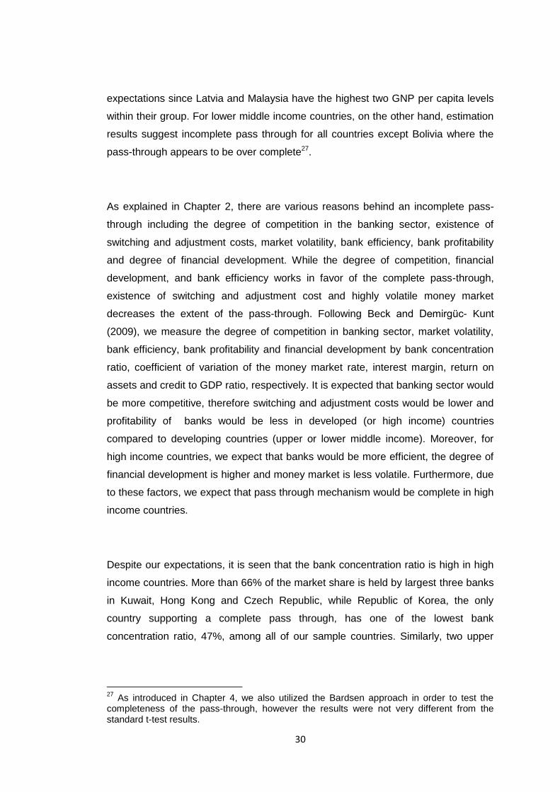
As explained in Chapter 2, there are various reasons behind an incomplete pass-

through including the degree of competition in the banking sector, existence of

switching and adjustment costs, market volatility, bank efficiency, bank profitability

and degree of financial development. While the degree of competition, financial

development, and bank efficiency works in favor of the complete pass-through,

existence of switching and adjustment cost and highly volatile money market

decreases the extent of the pass-through. Following Beck and Demirgüc- Kunt

(2009), we measure the degree of competition in banking sector, market volatility,

bank efficiency, bank profitability and financial development by bank concentration

ratio, coefficient of variation of the money market rate, interest margin, return on

assets and credit to GDP ratio, respectively. It is expected that banking sector would

be more competitive, therefore switching and adjustment costs would be lower and

profitability of banks would be less in developed (or high income) countries

compared to developing countries (upper or lower middle income). Moreover, for

high income countries, we expect that banks would be more efficient, the degree of

financial development is higher and money market is less volatile. Furthermore, due

to these factors, we expect that pass through mechanism would be complete in high

income countries.

Despite our expectations, it is seen that the bank concentration ratio is high in high

income countries. More than 66% of the market share is held by largest three banks

in Kuwait, Hong Kong and Czech Republic, while Republic of Korea, the only

country supporting a complete pass through, has one of the lowest bank

concentration ratio, 47%, among all of our sample countries. Similarly, two upper

27

As introduced in Chapter 4, we also utilized the Bardsen approach in order to test the completeness of the pass-through, however the results were not very different from the standard t-test results.

31

middle income countries, Malaysia28 and Latvia suggest a complete pass-through

with bank concentration ratios of 44% and 54%, respectively.

In line with our expectations, net interest margins are very low for the countries that

we found complete pass-through (Republic of Korea, Latvia, Malaysia) indicating

higher bank efficiency promoting the completeness of the process. Moreover, credit

to GDP ratio is very high for these countries (117% for Republic of Korea and 112%

for Malaysia), which represents the high usage of credits by agents in these

economies speeding up the IPT mechanism. Furthermore, low market volatility

appears to be another reason for completeness of IPT. Malaysia and Republic of

Korea have the lowest market volatility among all fifteen countries. For instance, the

market volatility in Malaysia is four times less than the market volatility in Hong

Kong.

Next we consider the high income countries for which estimation results have shown

incompleteness of IPT, namely; Kuwait, Hong Kong, Croatia and Czech Republic.

Contrary to the cases in Republic of Korea, Latvia and Malaysia, the indicators we

employ suggest slower adjustment of retail rates and incomplete IPT. To begin with,

the market volatility is high in all of these countries. Even though, the market

volatility in Czech Republic (0.52) is less than Kuwait, Hong Kong or Croatia, it is

twice the volatility in Republic of Korea and almost three times more than the

volatility in Malaysia. Moreover, Czech Republic (41%), Croatia (54%) and Kuwait

(61%) have a lower level of financial development when compared to Republic of

Korea (117%) and Malaysia (112%). When we take bank profitability indicator into

account the results are much or less the same. Hong Kong and Kuwait have the

largest return on assets ratio among all fifteen countries arising as a possible reason

for incompleteness of IPT since profitability (market power) has negative effect on

speed of pass through.

28

Malaysia has the lowest bank concentration ratio among our sample countries. See appendix for more detail.

32

For middle income countries suggesting incomplete pass through, overall, the

market volatility is high, financial development and bank efficiency are very low.

Therefore, it is not surprising to observe incomplete pass through in these middle

income countries. However, Bolivia appears to be an exceptional with an over

complete pass through. De Bondt (2005) argues that if the number of risky

borrowers or projects is high; banks adjust very quickly to increases in the money

market rate (or the official rate) in order to compensate for the risk of default on

loans. Hence sensitiveness of banks to changes in the money market rate due to

the risk factor could be an explanation for the over completeness of IPT in Bolivia.

Having discussed the estimates of the long-run equilibrium equation (1), we can

proceed with the results of the Engle-Granger cointegration test together with the

TAR and MTAR type cointegration tests of Enders and Siklos (2001). Tables 4, 5

and 6 present the results for high, upper middle and lower middle income countries,

respectively.

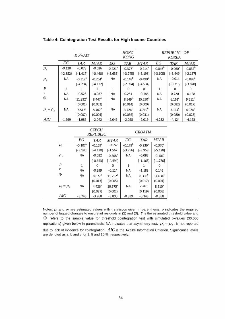
According to the Engle-Granger test, the null hypothesis of no cointegration is

rejected at the 5% significance level for high income countries, Hong Kong, Republic

of Korea and Croatia for upper middle income countries, Peru, and Thailand and for

lower-middle income countries Ukraine, Armenia, Philippines and Bolivia. It fails to

provide a significant cointegration for the countries Sri Lanka, Latvia, Malaysia,

Dominican Republic, Kuwait and Czech Republic. As discussed in Chapter 4, the

Engle-Granger methodology assumes symmetric adjustment and therefore might

produce misleading results if the adjustment is in fact asymmetric. For that reason

we continue with TAR and MTAR type cointegration testing procedures that account

for asymmetries in the adjustment process.

Estimating the equation (3) with the Heaviside indicator functions (4) and (5), we

perform TAR and MTAR type cointegration tests, respectively. At the 5%

33

significance level, based on the F test, , and corresponding simulated p-values29,

the TAR type cointegration test rejects the null hypothesis of no cointegration,

1 2 0, for the countries Republic of Korea, Malaysia, Peru, Thailand, Ukraine,

Armenia, Philippines. However, it fails to support cointegration inferences of the

standard Engle-Granger test for Bolivia and Republic of Korea. For the countries

supporting TAR type cointegration, we continue with testing the null of symmetric

adjustment 1 2 by a standard F-test. The results provide empirical support for

asymmetric adjustment (at the 5% level) for Thailand and (at the 10% level) for

Republic of Korea and Philippines Moving on to the MTAR cointegration test,

equations (3) and (5), we observe that existence of the cointegration between the

lending rate and the money market rate is strongly supported for all countries.

Furthermore, the null hypothesis of symmetric adjustment, 1 2 , is rejected for all

cases at the 5% level with the exception being Thailand and Armenia. While we fail

to detect asymmetric adjustment for Armenia, evidence of asymmetry is supported

at the 10% level with the p-value of 0.060 for Thailand. The consistent estimator of

the threshold value, , is close to zero in almost all countries demonstrating

asymmetric adjustment. Therefore, the adjustment speed depends on the sign of the

change in the ECT ( 1ˆ

tu ). However, for Latvia and Bolivia the estimated thresholds

are -1.676 and 1.180, respectively. Hence adjustment will have more momentum in

one direction than other depending on these values. Moreover, based on the Akaike

Information Criterion (AIC), the MTAR model appears to be the most appropriate

model for all countries30, except Hong Kong and Republic of Korea, for which TAR

and Engle-Granger models gives the best fit, respectively. However, for Hong Kong

we prefer to continue with the MTAR type adjustment since null hypothesis of no

cointegration rejected with a lower significance level when the MTAR type

asymmetry is allowed.

29

In order to employ exact critical values for our sample size and the augmentation order of (3), we perform a Monte Carlo simulation following Enders and Siklos (2001) and provide simulated p-values.

30 We choose MTAR model to describe the cointegration relation between the lending rate

and the money market rate in Sri Lanka. EG and TAR methodologies could not detect cointegration relation, however, at the 10% significance level these two rates are asymmetrically cointegrated according to MTAR model cointegration test results.

34

-0.128 -0.078 -0.026 -0.221b -0.377a -0.214a -0.046b -0.060a -0.032b

{-2.852} [-1.417] [-0.460] {-3.636} [-3.745] [-3.198] {-3.605} [-3.449] [-2.167]

NA -0.312a -0.264a NA -0.148b -0.490a NA -0.014 -0.098a

[-4.704] [-4.122] [-2.094] [-4.534] [-0.716] [-3.828]

2 1 2 1 0 0 1 0 0

NA -0.528 -0.037 NA 0.254 -0.186 NA 0.720 -0.128

NA 11.832a 8.447b NA 8.549b 15.290a NA 6.161c 9.611b

(0.001) (0.033) (0.014) (0.000) (0.082) (0.017)

NA 7.512a 8.407a NA 3.724c 4.719b NA 3.114c 4.924b

(0.007) (0.004) (0.056) (0.031) (0.080) (0.028)

-1.999 -1.986 -2.042 -2.046 -2.058 -2.019 -4.232 -4.124 -4.193

-0.107b -0.169a -0.057 -0.179b -0.236a -0.370a

{-3.186} [-4.130] [-1.567] {-3.756} [-3.958] [-5.128]

NA -0.032 -0.308a NA -0.088 -0.104c

[-0.643] [-4.494] [-1.168] [-1.780]

1 0 0 1 1 0

NA -0.399 -0.114 NA -1.188 0.146

NA 8.677b 11.252a NA 8.308b 14.634a

(0.013) (0.005) (0.017) (0.001)

NA 4.426b 10.375a NA 2.461 8.210a

(0.037) (0.002) (0.119) (0.005)

-3.746 -3.768 -3.800 -0.339 -0.343 -0.358

KUWAITHONG

KONGREPUBLIC OF

KOREA

EG TAR MTAR EG TAR MTAR EG TAR MTAR

1

2

p

1 2

AIC

CZECHREPUBLIC

CROATIA

EG TAR MTAR EG TAR MTAR

1

2

p

1 2

AIC

Table 4: Cointegration Test Results for High Income Countries

Notes: ρ1 and ρ2 are estimated values with t statistics given in parenthesis. p indicates the required number of lagged changes to ensure iid residuals in (2) and (3). is the estimated threshold value and

refers to the sample value for threshold cointegration test with simulated p-values (30.000

replications) given below in parenthesis. NA indicates that asymmetry test, 1 2 , is not reported

due to lack of evidence for cointegration. AIC is the Akaike Information Criterion. Significance levels

are denoted as a, b and c for 1, 5 and 10 %, respectively.

35

Table 5: Cointegration Test Results for Upper Middle Income Countries






-0.154 -0.213a -0.100c -0.019 -0.037a -0.065a -0.094 -0.069 -0.299a

{-3.032} [-3.516] [-1.852] {-2.815} [-4.674] [-4.184] {-2.765} [-1.466] [-4.795]

NA -0.026 -0.506a NA 0.015 -0.008 NA -0.119b -0.041

[-0.296] [-3.536] [1.397] [-1.015] [-2.536] [-1.060]

1 1 1 3 3 3 2 2 3

NA -2,456 -1,676 NA 0.238 0.035 NA -3,696 0.588

NA 6.165c 8.158b NA 11.848a 9.495b NA 4,089 11.843a

(0.081) (0.044) (0.001) (0.016) (0.295) (0.004)

NA 3.072c 6.826b NA NA 10.598a NA 0.608 12,564

(0.082) (0.010) (0.001) (0.437) (0.000)a

1,340 1,332 1,307 -5,243 -5,330 -5,301 0.803 0.812 0.720

-0.154b -0.195 -0.102b -0.078a -0.101a -0.094a

{-3.796} [-3.630] [-2.443] {-5.943} [-6.953] [-3.554]

NA -0.103 -0.499a NA -0.003 -0.038a

[-1.752] [-4.840] [-0.121] [-2.701]

1 1 1 0 0 0

NA 3,007 -0.488 NA -0.795 0.032

NA 7.854b 14.229a NA 24.015a 9.898b

(0.024) (0.000) (0.000) (0.014)

NA 1,362 12.988a NA 10.751a 3.590c

(0.245) (0.000) (0.001) (0.060)

0.606 0.610 0.535 -3,780 -3,836 -4,025

LATVIA MALAYSIADOMINICANREPUBLIC


1

2

p

1 2

AIC

PERU THAILANDEG TAR MTAR EG TAR MTAR

1

2

p

1 2

AIC

36

-0.201b -0.175a -0.119c -0.410a -0.419a -0.371a -0.097 -0.016 -0,019

{-3.675} [-2.951] [-1.732] {-5.371} [-5.132] [-4.162] {-1.790} [-0.236] [-0,303]

NA -0.295a -0.328a NA -0.352a -0.428a NA -0.234a -0.307a

[-2.922] [-4.944] [-3.146] [-4.360] [-3.164] [-3.647]

5 5 4 2 1 1 4 5 5

NA -4.656 -0.080 NA 1.209 -1.822 NA 2.045 -0.675

NA 7.321b 12.747a NA 16.695a 16.659a NA 4.973 6,605c

(0.029) (0.002) (0.000) (0.000) (0.154) (0.099)

NA 1.213 5.426b NA 0.257 0.198 NA 5.063b 8,222a

(0.273) (0.021) (0.613) (0.657) (0.026) (0.005)

2.824 2.829 2.802 2.130 2.129 2.129 0.704 0.661 0.639

-0.276b -0.407a -0.495a -0.240b -0.270a -0.366a

{-3.901} [-4.060] [-4.654] {-3.547} [-3.306] [-4.097]

NA -0.172c -0.144c NA -0.184c -0.094

[-1.913] [-1.697] [-1.714] [-0.986]

1 1 1 1 1 1

NA 0.743 0.440 NA -2.102 1.180

NA 9.344a 11.539a NA 6.445c 8.644b

(0.009) (0.004) (0.065) (0.033)

NA 3.332c 7.315a NA 0.440 4.496b

(0.070) (0.008) (0.508) (0.036)

-0.594 -0.603 -0.629 3.207 3.218 3.190

UKRAINE ARMENIA SRI LANKA


1

2

p

1 2

AIC

PHILIPPINES BOLIVIA

EG TAR MTAR EG TAR MTAR

1

2

p

1 2

AIC

Table 6: Cointegration Test Results for Lower Middle Income Countries






37

Discussion of the estimated speed of adjustments requires more attention, as they

will uncover the nature of the pass through. In this sense, we will discuss them first

on a country specific base (Section 5.1.1), and then accounting for the possible

income effect, we will provide a discussion across the income groups (Section

5.1.2).

5.1.1 Country Specific Results

As discussed in Chapter 2, existence of switching and searching costs is one of the

possible reasons to expect asymmetric adjustment of retail rates. These costs are

higher for banks and customers if banks are operating in a less competitive

environment. High degree of competition in banking sector may force banks to act

slower (faster) to increases (decreases) in the money market rate, indicating upward

stickiness of lending rates. Market volatility is another factor that may cause

asymmetric adjustment. Higher market volatility implies frequent and sharp changes

in official rate which creates shocks to banking sector leading to uncertainty and

asymmetric information problems. Hence, in order to avoid short-run losses, banks

may act slowly when decreasing their lending rates, initiating downward stickiness of

the lending rates. Beside these factors, collusive pricing arrangement and adverse

customer reaction hypothesis may explain the downward and upward stickiness of

lending rates respectively.

Regarding the speed of adjustments observed from MTAR type cointegration, it is

seen that Ukraine lending rates respond more to money market rate changes when

change in the ECT is positive. Payne (2007) argues that negative realizations of the

change in ECT stem from the rise in the money market rate which in turn decreases

the gap between the lending rate and the money market rate. Therefore, negative

changes in ECT point to increases in the money market rate.

Figure 4,5 and 6 plots the changes in the ECT along with the estimated threshold

value for high income, upper middle income and lower middle income countries,

38

-3

-2

-1

0

1

2

3

99 00 01 02 03 04 05 06 07 08 09 10 11

Change in ECT threshold value

KUWAIT

-1.5

-1.0

-0.5

0.0

0.5

1.0

1.5

99 00 01 02 03 04 05 06 07 08 09 10 11


HONG KONG

-0.8

-0.4

0.0

0.4

0.8

1.2

1.6

99 00 01 02 03 04 05 06 07 08 09 10 11


CZECH REPUBLIC

-4

-2

0

2

4

6

99 00 01 02 03 04 05 06 07 08 09 10 11


CROATIA

respectively. Being in line with the estimated speed of adjustment coefficients,

Figure 6 illustrates that negative changes in the ECT dies quicker compared to

positive changes for Ukraine. This clearly implies that Ukraine lending rate follows

money market rate increases closely, while they are reluctant to follow declines in

the money market rate. High market volatility (highest among all countries),

uncertainty about the market and high inflation rate could be possible reasons

behind this downward rigidity.

FIGURE 4: Change in the Error-Correction Term Series of High Income

Countries

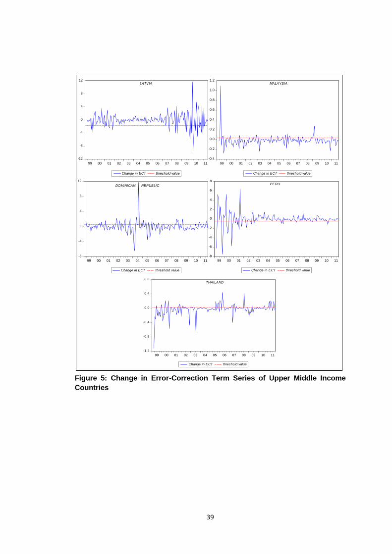
39

-12

-8

-4

0

4

8

12

99 00 01 02 03 04 05 06 07 08 09 10 11


LATVIA

-8

-4

0

4

8

12

99 00 01 02 03 04 05 06 07 08 09 10 11


DOMINICAN REPUBLIC

-8

-6

-4

-2

0

2

4

6

8

99 00 01 02 03 04 05 06 07 08 09 10 11


PERU

-0.4

-0.2

0.0

0.2

0.4

0.6

0.8

1.0

1.2

99 00 01 02 03 04 05 06 07 08 09 10 11


MALAYSIA

-1.2

-0.8

-0.4

0.0

0.4

0.8

99 00 01 02 03 04 05 06 07 08 09 10 11


THAILAND

Figure 5: Change in Error-Correction Term Series of Upper Middle Income

Countries

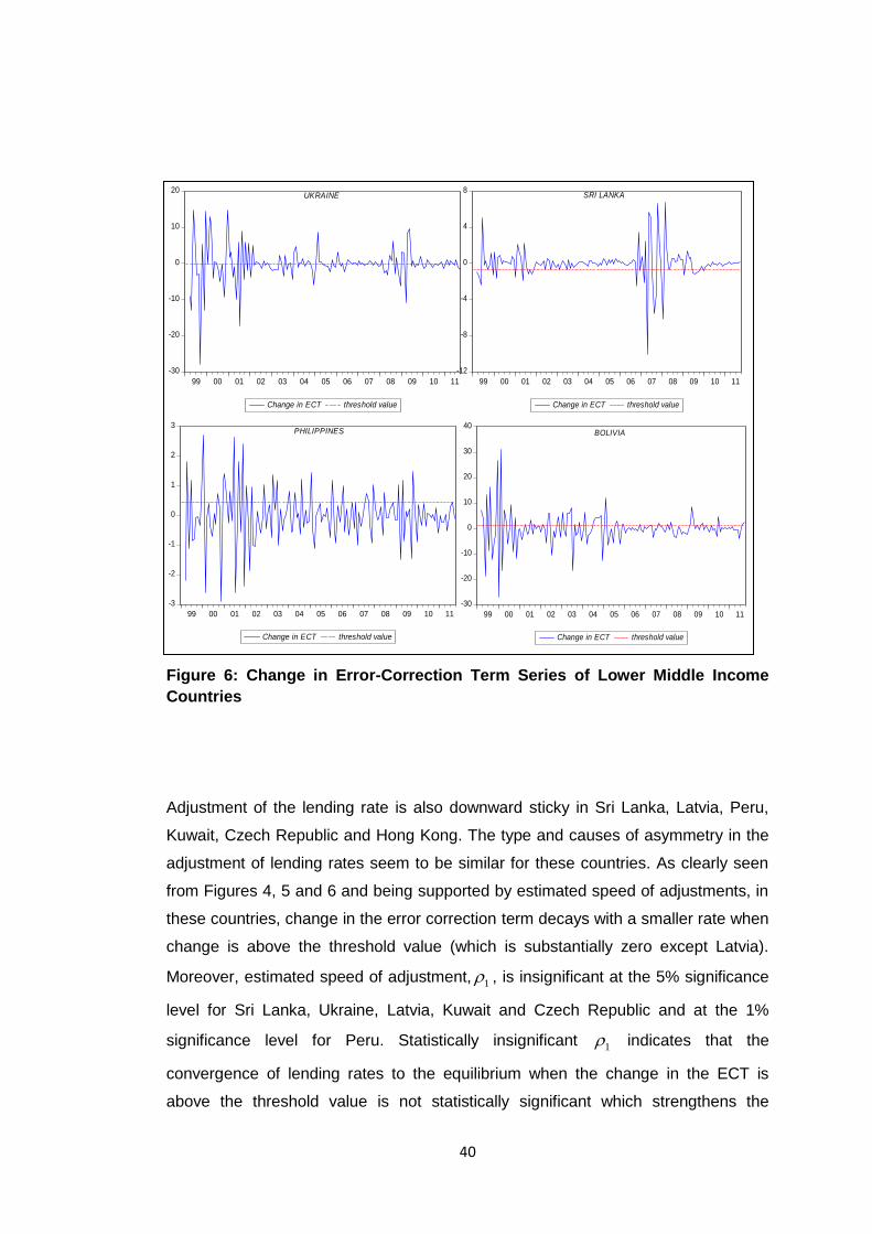
40

-30

-20

-10

0

10

20

99 00 01 02 03 04 05 06 07 08 09 10 11


UKRAINE

-30

-20

-10

0

10

20

30

40

99 00 01 02 03 04 05 06 07 08 09 10 11


BOLIVIA

-12

-8

-4

0

4

8

99 00 01 02 03 04 05 06 07 08 09 10 11


SRI LANKA

-3

-2

-1

0

1

2

3

99 00 01 02 03 04 05 06 07 08 09 10 11


PHILIPPINES

Figure 6: Change in Error-Correction Term Series of Lower Middle Income

Countries

Adjustment of the lending rate is also downward sticky in Sri Lanka, Latvia, Peru,

Kuwait, Czech Republic and Hong Kong. The type and causes of asymmetry in the

adjustment of lending rates seem to be similar for these countries. As clearly seen

from Figures 4, 5 and 6 and being supported by estimated speed of adjustments, in

these countries, change in the error correction term decays with a smaller rate when

change is above the threshold value (which is substantially zero except Latvia).

Moreover, estimated speed of adjustment, 1 , is insignificant at the 5% significance

level for Sri Lanka, Ukraine, Latvia, Kuwait and Czech Republic and at the 1%

significance level for Peru. Statistically insignificant 1 indicates that the

convergence of lending rates to the equilibrium when the change in the ECT is

above the threshold value is not statistically significant which strengthens the

41

downward stickiness of lending rates in these countries. Main cause of this type of

asymmetry seems to be the fact that the banking sector is highly concentrated in

most of these countries except Latvia. Banks in these countries have noticeable

market power which enables them to adapt to the increases in the money market

rate more quickly compared to the decreases. Moreover, high market volatility in

Hong Kong and Peru and Latvia supports the downward sluggishness of lending

rates in these countries. Among the countries for which we observe downward

sluggishness of lending rates, Latvia is the only country having a threshold value

substantially different from zero (-1.676). It seems that for Latvia, the speed of

adjustment increases when the increase in the money market rate is above a certain

level. Hence, we can deduce that banks in Latvia act slowly to small changes in the

money market rate, but act faster when increase in money market rate is noticeably

large. High and relatively unstable inflation may the hidden cause of such

asymmetry.

Unlike the countries discussed above, we observe upward stickiness of lending

rates in Philippines, Malaysia, Thailand, Dominican Republic, Croatia and Bolivia.

Figures 4, 5 and 6 depict the fact that positive deviations from the equilibrium are

eliminated quickly, which is also supported by estimated speed of adjustments with

faster adjustment following positive changes in the ECT. Moreover, the speed of

adjustment when the change in ECT is below the threshold value, 2 , is statistically

insignificant at the 10% significance level for Bolivia, Malaysia, Dominican Republic

and at the 5% significance level for Philippines and Croatia. Insignificance of 2

supports our finding in terms of upward stickiness in these countries since

adjustment of lending rates to increases in the money market rate is statistically

insignificant. Upward stickiness of lending rates may be attributed to high degree of

competition in Malaysia, Thailand, Croatia and Bolivia whereas it may be attributed

to low market volatility in Philippines, and Dominican Republic. As discussed in

chapter 2, we expect lower profitability of banks if the degree of competition in

banking sector is high which in turn indicates that banks have low market power. In

the light of this peculiar expectation and corresponding to it, bank concentration ratio

is widely used in the literature in order to measure the degree of competition.

However, we cannot ignore the fact that banks may operate in competitive market

even though the concentration is high. Therefore, we take the profitability of banks in

42

Dominican Republic in consideration in order to make sure that high concentration

results from less competition. Profitability of banks in Dominican Republic is very

low31 which may be due to high competition in banking sector, supporting the

upward rigidity of the lending rate. Among these countries Bolivia is unique in terms

of estimated threshold value which is substantially positive. The positive threshold

indicates that adjustment is faster following large decreases in the money market

are realized. Integrating the over completeness of the IPT mechanism in Bolivia into

the discussion, it is possible that Bolivian banks not only pass the increases in the

money market rate to the lending rate, but also increase the markups on the lending

rate. Larger markups prevent losses that would occur due to sudden increases in

the money market rate which may be the reason for banks to act slowly to small

decreases and any increase in the money market rate. Moreover, due to high

inflation, banks in Bolivia anticipate increases rather than decreases in the money

market rate, hence, they hesitate to adjust to small decreases and wait for a

noticeable decrease in the money market rate. When a relatively large fall in the

money market rate is realized, banks act faster due to the high degree of

competition among banks.

When we consider the collusive pricing arrangements and adverse customer

reaction hypothesis, the downward rigidity of lending rates in Ukraine, Peru, Latvia32,

Czech Republic, Hong Kong33 and Kuwait is supported by collusive pricing

arrangements theory, whereas upward rigidity of lending rates in Philippines, Bolivia,

31

Lowest among all countries. Profitability measured by returns on assets.

32 Sander and Kleimeier (2004b), Crespo-Cuaresma et al (2004) and Amarasekara (2005)

find symmetric adjustment of lending rates in Latvia, Czech Republic and Sri Lanka respectively, while we uncover significant asymmetries for these countries. The type of loans under consideration, sample periods and the methodology utilized may have caused differences in findings.

33 Our inference in favor of downward rigidity of the lending rates in Hong Kong is in line with

the MTAR approach of Wang and Lee (2009), though some substantial differences regarding other countries remain. While they fail to find significant cointegration between the lending rates and the money market rate for Thailand, Republic of Korea and Malaysia, we provide strong empirical evidences for cointegration. Moreover, contrary to our findings, they conclude that Philippines’ lending rates exhibit downward rigidities. The possible reason for these different inferences could be simply the sample period employed.

43

Thailand, Dominican Republic, Malaysia and Croatia is supported by the adverse

customer reaction theory. It is worth to note that Republic of Korea and Armenia are

the only countries with symmetric34 IPT mechanism according to our estimation

results.

5.1.2. Results for Country Income Groups

As discussed in chapter 2, inflation has positive impact on the speed of adjustment.

From tables 4, 5 and 6, we realize that speeds of adjustment parameters are higher

for especially lower middle income group countries. Adjustment of lending rates to

changes in the money market rate seems to be faster for Latvia, Peru and

Dominican Republic within upper middle income group confirming the positive effect

of inflation on pass through. On the other hand, inflation rate is lower for high

income countries as a group. However, all countries except Republic of Korea

experience relatively quick adjustment of rates. Contrary to other income groups,

most outstanding reason to find speedier adjustment in these countries is the high

level of income since GDP per capita, which is expected to increase the speed of

pass through as indicated by Gigineshvili (2011). In addition, highly developed

financial sector seems to increase the speed of pass through in Croatia, Hong Kong

and Kuwait, while low level of market volatility boosts the speed of adjustment in

Czech Republic. Among our sample countries, lending rates in Malaysia, Thailand

and Republic of Korea seem to adjust slower in both directions compared to other

countries despite the positive effect of low market volatility, low concentration and

high level of financial development. The inflation rate is low in all these three

countries. One possible explanation for low speed of adjustment could be the menu

costs. Banks in these countries wait long enough to change their rates to avoid

adjustment costs such as cost of advertising, printing menus, labor time devoted for

the adjustments.

34

As discussed in Chapter 2, insignificant switching and searching costs, high level of

competition, perfect information about the market conditions may produce symmetric adjustments in these countries. Comparison of the speed of adjustments suggests that the IPT process works faster in Armenia. High inflationary environment may force Armenian banks to change their rates quickly whereas Korean banks act slowly due to menu costs caused by the low level of inflation.

44

As shown in figures 4-6, we observe that threshold cuts only large spreads of the

changes in the ECT for almost all countries35 which indicates that the speed of

adjustment is speedier when there is a large change in the ECT whether it is

positive or not36. Hence, size of the change in the money market rate is as important

as the sign of the change in terms of effectiveness of the monetary policy. Small

increases or decreases in the official rate (or the money market rate) will not have

significant impact on the lending rate especially in short-run. When we consider the

figures 4-6, it is clear to see that spreads are wider in lower middle income

countries. Due to high inflation, policy makers need to take more drastic measures.

When we consider the type of asymmetry (downward or upward rigidity) results, we

observe that income level plays only a marginal role in explanation of the type of

asymmetry. Taking market structures into consideration, we expect upward

stickiness of lending rates in high income countries. However, high income level

does not guarantee high level of financial development, high level of competition

among banks or low market volatility. Due to these conditions, we find upward

rigidity in some lower income countries such as Bolivia and Malaysia, while we

observe downward rigidity in most of the high income countries; Hong Kong, Kuwait,

Czech Republic. Hence, even though countries are homogenous in terms of income

level within their group, they are not homogenous in terms of financial and

macroeconomic indicators.

Having established the MTAR type cointegration between the lending rate and the

money market rate for all countries (except Republic of Korea and Armenia), we

continue with estimation of MTAR type nonlinear ECMs given in (6) and (7) with the

indicator function (5) and the consistent estimate of the threshold value presented

in Tables 6, 7 and 8.

35

Size of the change in the ECT seems to have marginal effect in Ukraine and Kuwait.

36 Similar to findings of Sznajderska (2012) for Poland

45

5.2. Threshold ECM Results

The speed of adjustment parameters 1 and 2 obtained from the MTAR model and

given in Tables 4, 5 and 6 are in line with the error correction terms ( 1 and 2 )

observed from the nonlinear threshold ECM models presented in Tables 7, 8 and 9

for all countries37. Hence, as expected, all inferences discussed in detail in the

previous section are valid for threshold ECMs.

As mentioned before, our single equation modeling relies on the weak exogeneity

assumption of the money market rate to the lending rate. This assumption is

satisfied when the error-correction term does not have a significant impact on

changes in the money market rate; namely when 1 and 2 are statistically

insignificant in the money market rate equations. Our results support the weak

exogeneity of the money market rate at the 5% significance level38.

Moreover, as seen in Tables 7 – 9; the null hypothesis 0 1 ... 0pH could

be rejected at the 1% significance level for Thailand, Ukraine, and Sri Lanka and at

the 5% significance level for Hong Kong when the ECM model presented by

equation (7) is estimated. This indicates that, the lending rate granger causes the

money market rate in the short-run only for Thailand, Ukraine, Sri Lanka and Hong

Kong. However, these results do not indicate that the money market is determined

by the lending rate but imply that changes in the money market rate may be affected

37

The exceptions are Ukraine and Hong Kong.

38 Estimated speed of adjustment coefficient is significant at the 5% level in Dominican

Republic, however, the estimated value is positive which indicates that the money market rate does not converge to an equilibrium, suppoting the weak exogeneity of the money market rate. On the other hand, the money market rate in Latvia converges to the equilibrium when change in ECT is below the threshold value. A bi-variate model instead of a uni-variate model may fit better to interest rate pass through analysis of Latvia.

46

by the changes in the lending rate in the short-run, without violating the weak

exogeneity of the money market rate39.

39

See Engle et al. (1983) for further information

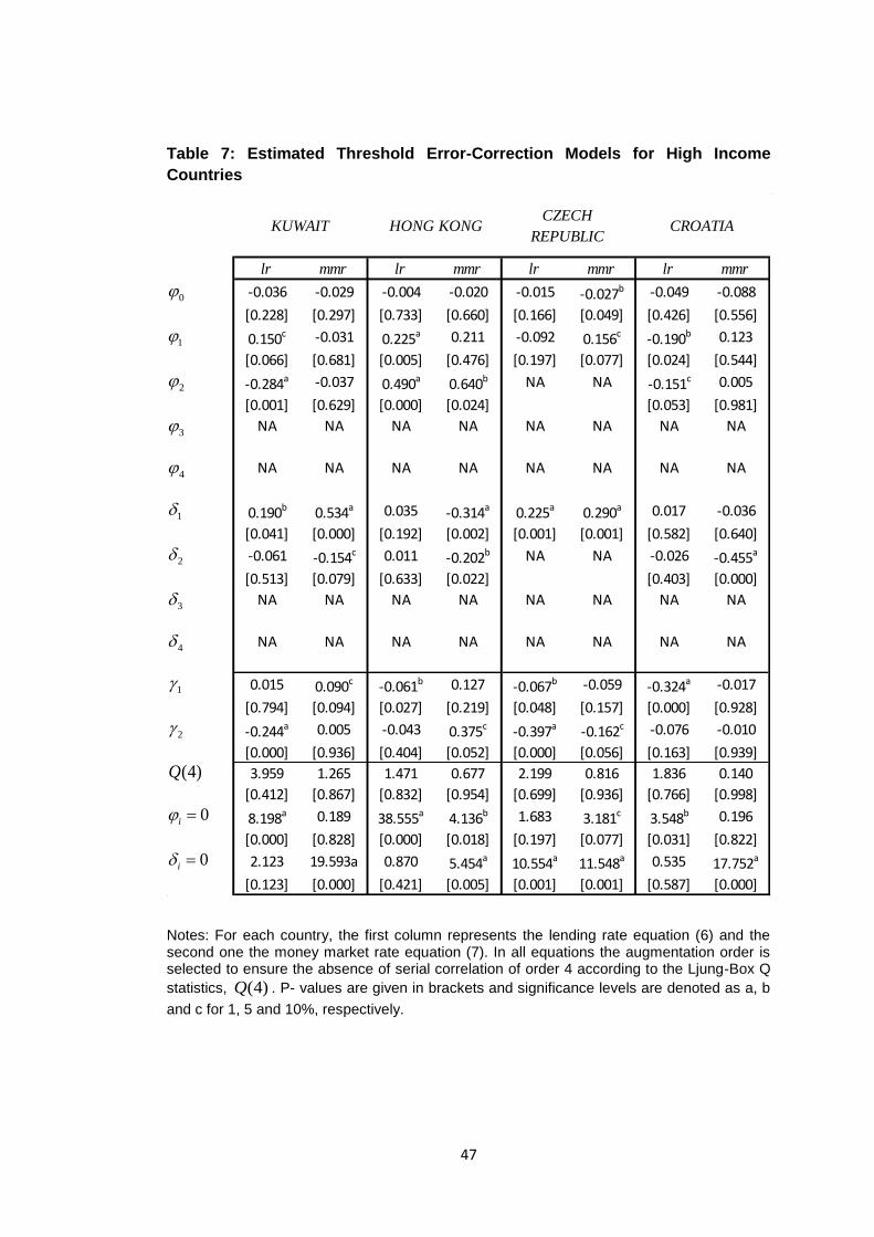
47

lr mmr lr mmr lr mmr lr mmr

-0.036 -0.029 -0.004 -0.020 -0.015 -0.027b -0.049 -0.088

[0.228] [0.297] [0.733] [0.660] [0.166] [0.049] [0.426] [0.556]

0.150c -0.031 0.225a 0.211 -0.092 0.156c -0.190b 0.123

[0.066] [0.681] [0.005] [0.476] [0.197] [0.077] [0.024] [0.544]

-0.284a -0.037 0.490a 0.640b NA NA -0.151c 0.005

[0.001] [0.629] [0.000] [0.024] [0.053] [0.981]

NA NA NA NA NA NA NA NA


0.190b 0.534a 0.035 -0.314a 0.225a 0.290a 0.017 -0.036

[0.041] [0.000] [0.192] [0.002] [0.001] [0.001] [0.582] [0.640]

-0.061 -0.154c 0.011 -0.202b NA NA -0.026 -0.455a

[0.513] [0.079] [0.633] [0.022] [0.403] [0.000]



0.015 0.090c -0.061b 0.127 -0.067b -0.059 -0.324a -0.017

[0.794] [0.094] [0.027] [0.219] [0.048] [0.157] [0.000] [0.928]

-0.244a 0.005 -0.043 0.375c -0.397a -0.162c -0.076 -0.010

[0.000] [0.936] [0.404] [0.052] [0.000] [0.056] [0.163] [0.939]

3.959 1.265 1.471 0.677 2.199 0.816 1.836 0.140

[0.412] [0.867] [0.832] [0.954] [0.699] [0.936] [0.766] [0.998]

8.198a 0.189 38.555a 4.136b 1.683 3.181c 3.548b 0.196

[0.000] [0.828] [0.000] [0.018] [0.197] [0.077] [0.031] [0.822]

2.123 19.593a 0.870 5.454a 10.554a 11.548a 0.535 17.752a

[0.123] [0.000] [0.421] [0.005] [0.001] [0.001] [0.587] [0.000]

CZECH

REPUBLIC CROATIAKUWAIT HONG KONG

0

1

2

3

4

1

2

3

4

1

2

(4)Q

0i

0i

Table 7: Estimated Threshold Error-Correction Models for High Income

Countries

Notes: For each country, the first column represents the lending rate equation (6) and the second one the money market rate equation (7). In all equations the augmentation order is selected to ensure the absence of serial correlation of order 4 according to the Ljung-Box Q

statistics, (4)Q . P- values are given in brackets and significance levels are denoted as a, b

and c for 1, 5 and 10%, respectively.

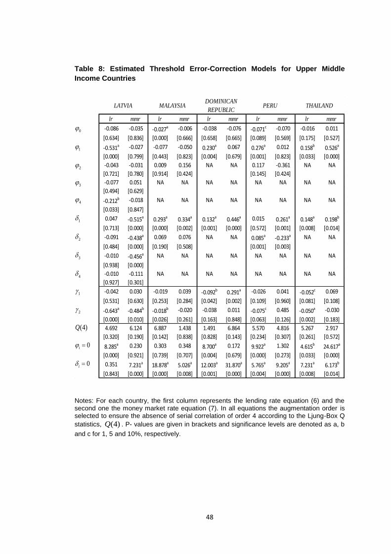
48

lr mmr lr mmr lr mmr lr mmr lr mmr

-0.086 -0.035 -0.027a -0.006 -0.038 -0.076 -0.071c -0.070 -0.016 0.011

[0.634] [0.836] [0.000] [0.666] [0.658] [0.665] [0.089] [0.569] [0.175] [0.527]

-0.531a -0.027 -0.077 -0.050 0.230a 0.067 0.276a 0.012 0.158b 0.526a

[0.000] [0.799] [0.443] [0.823] [0.004] [0.679] [0.001] [0.823] [0.033] [0.000]

-0.043 -0.031 0.009 0.156 NA NA 0.117 -0.361 NA NA

[0.721] [0.780] [0.914] [0.424] [0.145] [0.424]

-0.077 0.051 NA NA NA NA NA NA NA NA

[0.494] [0.629]

-0.212b -0.018 NA NA NA NA NA NA NA NA

[0.033] [0.847]

0.047 -0.515a 0.293a 0.334a 0.132a 0.446a 0.015 0.261a 0.148a 0.198b

[0.713] [0.000] [0.000] [0.002] [0.001] [0.000] [0.572] [0.001] [0.008] [0.014]

-0.091 -0.438a 0.069 0.076 NA NA 0.085a -0.233a NA NA

[0.484] [0.000] [0.190] [0.508] [0.001] [0.003]

-0.010 -0.456a NA NA NA NA NA NA NA NA

[0.938] [0.000]

-0.010 -0.111 NA NA NA NA NA NA NA NA

[0.927] [0.301]

-0.042 0.030 -0.019 0.039 -0.092b 0.291a -0.026 0.041 -0.052c 0.069

[0.531] [0.630] [0.253] [0.284] [0.042] [0.002] [0.109] [0.960] [0.081] [0.108]

-0.643a -0.484b -0.018b -0.020 -0.038 0.011 -0.075c 0.485 -0.050a -0.030

[0.000] [0.010] [0.026] [0.261] [0.163] [0.848] [0.063] [0.126] [0.002] [0.183]

4.692 6.124 6.887 1.438 1.491 6.864 5.570 4.816 5.267 2.917

[0.320] [0.190] [0.142] [0.838] [0.828] [0.143] [0.234] [0.307] [0.261] [0.572]

8.285a 0.230 0.303 0.348 8.700a 0.172 9.922a 1.302 4.615b 24.617a

[0.000] [0.921] [0.739] [0.707] [0.004] [0.679] [0.000] [0.273] [0.033] [0.000]

0.351 7.231a 18.878a 5.026a 12.003a 31.870a 5.765a 9.205a 7.231a 6.173b

[0.843] [0.000] [0.000] [0.008] [0.001] [0.000] [0.004] [0.000] [0.008] [0.014]

THAILANDLATVIA MALAYSIADOMINICAN

REPUBLIC PERU

0

1

2

3

4

1

2

3

4

1

2

(4)Q

0i

0i

Table 8: Estimated Threshold Error-Correction Models for Upper Middle

Income Countries




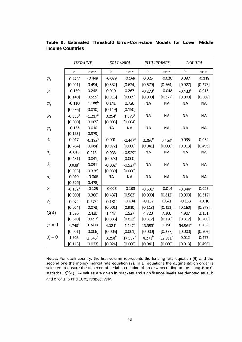
49

lr mmr lr mmr lr mmr lr mmr

-0.475a -0.449 -0.039 -0.169 0.025 -0.020 0.037 -0.118

[0.001] [0.494] [0.532] [0.624] [0.679] [0.564] [0.927] [0.276]

-0.129 0.248 0.010 0.267 -0.270a -0.048 -0.430a 0.013

[0.140] [0.555] [0.915] [0.605] [0.000] [0.277] [0.000] [0.502]

-0.110 -1.155b 0.141 0.726 NA NA NA NA

[0.236] [0.010] [0.119] [0.150]

-0.355a -1.217a 0.254a 1.376a NA NA NA NA

[0.000] [0.005] [0.003] [0.004]

-0.125 0.010 NA NA NA NA NA NA

[0.135] [0.979]

0.017 -0.192c 0.001 -0.447a 0.286b 0.468a 0.035 0.059

[0.464] [0.084] [0.972] [0.000] [0.041] [0.000] [0.913] [0.493]

-0.015 0.216b -0.038b -0.529a NA NA NA NA

[0.481] [0.041] [0.023] [0.000]

0.038c 0.091 -0.032b -0.527a NA NA NA NA

[0.053] [0.338] [0.039] [0.000]

0.019 -0.066 NA NA NA NA NA NA

[0.326] [0.478]

-0.152a -0.125 -0.026 -0.103 -0.531a -0.014 -0.344a 0.023

[0.000] [0.366] [0.437] [0.583] [0.000] [0.812] [0.000] [0.312]

-0.072b 0.275c -0.181a -0.034 -0.137 0.041 -0.133 -0.010

[0.024] [0.073] [0.001] [0.910] [0.113] [0.421] [0.160] [0.678]

1.596 2.430 1.447 1.527 4.720 7.200 4.907 2.151

[0.810] [0.657] [0.836] [0.822] [0.317] [0.126] [0.317] [0.708]

4.746a 3.743a 4.324a 4.247a 13.353a 1.190 34.561a 0.453

[0.001] [0.006] [0.006] [0.001] [0.000] [0.277] [0.000] [0.502]

1.903 2.946b 3.258b 17.597a 4.271b 32.911a 0.012 0.473

[0.113] [0.023] [0.024] [0.000] [0.041] [0.000] [0.913] [0.493]

UKRAINE SRI LANKA PHILIPPINES BOLIVIA

0

1

2

3

4

1

2

3

4

1

2

(4)Q

0i

0i

Table 9: Estimated Threshold Error-Correction Models for Lower Middle

Income Countries




50

CHAPTER 6

CONCLUSION

In this study we investigate the nature of the pass-through of the money market rate

to the lending rate in fifteen countries grouped as high income, upper middle income

and lower middle income within the context of univariate threshold error-correction

models. Our aim is to account for not only asymmetries but also possible

heterogeneities arising from income differences. The preliminary results reveal that

the pass-through from the money market rate to the lending rate is incomplete for all

countries except Republic of Korea, Latvia and Malaysia. Even though income level

in these countries are higher compared to most our sample countries, it seems that

income has only a marginal effect on the completeness of the pass-through

mechanism. We observe incomplete IPT in rest of our sample countries, possibly

due to high market volatility, low degree of competition in banking sector and lower

level of financial development.

TAR and MTAR cointegration tests uncover the crucial role of the nonlinearities in

our pass-through analysis, as it is observed that all lending rates adjust

asymmetrically following money market rate changes. Moreover, the MTAR type

nonlinear adjustment appears to be more appropriate than TAR type adjustment for

almost all cases except Republic of Korea and Armenia. Specifically, the loan rates

of Ukraine, Sri Lanka, Latvia, Peru, Kuwait, Hong Kong and Czech Republic

increase faster (slower) following a rise (fall) in the money market rate, whereas

lending rates in Bolivia, Philippines, Malaysia, Dominican Republic, Thailand and

Croatia exhibit upward sticky adjustment. Even though we expect upward

(downward) stickiness in high (middle) income countries, these findings indicate that

income does not have a substantial effect on the form of the asymmetry. Differences

in the financial market and macroeconomic conditions seem to be possible reasons

51

for differences within and between country groups in terms of asymmetric

adjustment of lending rates.

Overall, our results suggest that lending rates of the countries, where the degree of

competition is high (low) and bank profitability and market volatility are low (high),

exhibit upward (downward) stickiness. Unlike most of the studies in the literature, we

have tested both long-run and short-run dynamics of the IPT. Our empirical results

for threshold ECMs show that the weak exogeneity of the money market rate, which

is the basis of our univariate analysis, is satisfied.

In this study we considered only the pass through from the money market rate to the

lending rate. However, nature of the IPT to deposit rates is as important as loan

rates; therefore an important task for future research could be analyzing the

responses of deposit rates with different maturities. Another interesting direction for

future research on the interest rate pass through could be setting a multivariate

system with money market, lending and deposit rates and allowing for the

interactions between lending and deposit rates.

52

REFERENCES

Adams, R and Amel, D.F. (2011). “Market Structure and the Pass-Through of the

Federal Funds Rate”. Journal of Banking and Finance, 35, 5, 1087-96.

Amarasekara, C. (2005). “Interest Rate Pass-through in Sri Lanka”. Central Bank of

Sri Lanka Stuff Studies, 35, 1&2, 1-32.

Banerjee, A., J. J. Dolado, D. F Hendry, and G. W. Smith. (1986). “Exploring

Equilibrium Relationships in Econometrics Through Static Models: Some Monte

Carlo evidence”. Oxford Bulletin of Economics and Statistics, 48, 253-277.

Bardsen, G. (1989). “The Estimation of Long-run Coefficients from Error-Correction

Models”. Oxford Bulletin of Economics and Statistics, 51, 345-50.

Beck, T. and Demirgüc-Kunt, A. (2009). “Financial Institutions and Markets Across

Countries and Over Time: Data and Analysis”. World Bank Policy Research Working

Paper No. 4943.

Cecchin, I. (2011). “Mortgage Rate Pass-Through in Switzerland”. Swiss National

Bank Working Papers 2011-8.

Chan, K. (1993). “Consistency and Limiting Distribution of the Least Squares

Estimator of a Threshold Autoregressive Model”. Annals of Statistics, 21, 520-33.

Chan, K. S. and H. Tong (1990). “On Likelihood Ratio Tests for Threshold

Autoregression.” Journal of the Royal Statistical Society, Series B, 52, 469–476.

Chionis, D.P. and Leon C.A. (2006). “Interest Rate Transmission in Greece: Did

EMU Cause a Structural Break?”. Journal of Policy Modeling, 28, 453-66.

Cook, S. (2007). “A Threshold Cointegration Test with Increased Power”.

Mathematics and Computers in Simulation, 73 (6), 386-92.

53

Cottarelli, C. and Kourelis, A. (1994). “ Financial Structure, Bank Lending Rates, and

the Transmission Mechanism of Monetary Policy”. IMF Staff Papers, 41, 587-623.

Crespo-Cuaresma, J., Egert, B. and Reininger, T. (2004). “Interest Rate Pass-

Through in New EU States: The Case of the Czech Republic, Hungary and Poland”.

William Davidson Institute Working Paper 671.

De Bondt, G. (2005). “Interest Rate Pass-Through: Emprical Results for the Euro

Area”. German Economic Review, 6, 37-78.

Dueker, M. (2000). “Are Prime Rate Changes Asymmetric?”. Federal Reserve Bank

of St. Louis Review September/October, 33-40.

Egert, B., Crespo-Cuaresma, J. and Reininger, T. (2007). “Interest Rate Pass-

Through in Central and Eastern Europe: Reborn from Ashes Merely to Pass

Away?”. Journal of Policy Modeling, 29 (2), 209-25.

Enders, W. and Siklos, P. (2001). “ Cointegration and Threshold Adjustment”.

Journal of Business and Economic Statistics, 19, 166-76.

Engle, R., Hendry, D. and Richard J-F. (1983). “Exogeneity”. Econometrica, 51 (2),

277-304.

Engle, R. F. and Granger, C. W. J. (1987). “Co-integration and Error Correction:

Representation, Estimation and Testing”. Econometrica, 55, 251-276.

Freixas, X. and Rochet, J. D. (1997). “Microeconomics of Banking”. MIT Press,

Cambridge, MA.

Frisancho-Mariscal, I. B. and Howells, P. (2011). “Interest Rate Pass-Through and

Risk”. Economic Issues, 16 (2), 93-114.

Fuertes, A-M., Heffernan, S. and Kalotychou, E. (2010). “How do UK Banks React to

Changing Central Bank Rates?”. Journal of Financial Services Research , 37, 99-

130.

54

Gambacorta, L. and Iannotti, S. (2007). “Are There Asymmetries in the Response of

Bank Interest Rates to Monetary Shocks?”. (2007). Applied Economics, 39 (19),

2503-17.

Gigineishvili, N. (2011). “Determinants of the Interest Rate Pass-Through: Do

Macroeconomic Conditions and Financial Market Structure Matter?”. IMF Working

Paper 11/176.

Hannan, T. H. and Berger, A. N. (1991). “The Rigidity of Prices: Evidence from

Banking Industry”. American Economic Review, 81, 938-45.

Hansen, N-J. H. and Welz, P. (2011). “Interest Rate Pass-Through During Global

Financial Crisis: The Case of Sweden”. OECD Economics Department Working

Papers, 855.

Hofmann, B. (2006). “EMU and the Transmission of Monetary Policy: Evidence from

Business Lending Rates”. Emprica, 33 (4), 209-29.

Horvath, Cs., Kreko, J. and Naszodi, A. (2004). “Interest Rate Pass-Through: The

Case of Hungary”. National Bank of Hungary Working Paper 8.

IMF. (2012). International Financial Statistics. Retrieved from http://elibrary-

data.imf.org/QueryBuilder.aspx?key=19784651&s=322 (04.03.2012)

Jobst, C. and Kwapil, C. (2008). “The Interest Rate Pass-Through in Austria –

Effects of the Financial Crisis”. Monetary Policy and the Economy Q4/08, Vienna:

OeNB, 54-67.

Karagiannis, S., Panagopoulos, Y. And Vlamis, P. (2010). “Interest Rate Pass-

through in Europe and the US: Monetary Policy After the Financial Crisis”. Journal of

International Financial Markets, Institutions and Money, 20(5), 323-338.

55

Leuvensteijn, M., Bikker, J.A., Rixtel, A.A.R.J.M., and Sorensen, K.C. (2011). “A

new Approach to Measuring Competition in the Loan Markets of the Euro Area”.

Applied Economics, 43, 23, 3155-67.

Liu, M-H., Margaritis, D. and Tourani-Rad, A. (2008). “Monetary Policy

Transparency and Pass-Through of Retail Interest Rates”. Journal of Banking and

Finance, 32 (4), 501-11.

Lowe, P. and Rohling, T. (1992) “Loan Rate Stickiness: Theory and Evidence”.

Research Discussion Paper, Reserve Bank of Australia.

Mizen, P. and Hofmann B. (2002). “Base Rate Pass-Through: Evidence from Banks’

and Building Societies’ Retail Rates”. Working Paper 170, Bank of England.

Mojon, B. (2000). "Financial Structure and the Interest Channel of ECB Monetary

Policy". ECB Working Paper, No. 40

Neumark, D. and Sharpe, S. A. (1992). “Market Structure and the Nature of Price

Rigidity: Evidence from the Market for Consumer Deposits”. Quarterly Journal of

Economics, 107, 657-80.

Ng, S. and Perron, P. (2001). “Lag Length Selection and the Construction of Unit

Root Tests with Good Size and Power”. Econometrica, 69 (6), 1519-54.

Payne, J. (2006). “The Response of the Conventional Mortgage Rate to the Federal

Funds Rate: Symmetric or Asymmetric Adjustment?”. Applied Financial Economics

Letters, 2, 279-84.

Payne, J. (2007). “Interest Rate Pass-Through and Asymmetries in Adjustable Rate

Mortgages”. Applied Financial Economics, 17, 1369-76.

Payne, J. and Waters, G. A. (2008). “Interest Rate Pass-Through and Asymmetric

Adjustment: Evidence from the Federal Funds Rate Operating Target Period”.

Applied Economics, 40 (11), 1355-1362.

56

Sander, H. And Kleimeier, S. (2002). “Asymmetric Adjustment of Commercial Bank

Interest Rates in the Euro Area: An Emprical Investigation into Interest Rate Pass-

Through”. Kredit und Kapital, 35, 161-92.

Sander, H. and Kleimeier, S. (2004a). “Convergence in Euro-Zone Retail Banking?

What Interest Rate Pass-Through Tells Us about Monetary Policy Transmission,

Competition and Integration”. Journal of International Money and Finance, 23 (3),

461-492.

Sander, H. and Kleimeier, S. (2004b). Interest Rate Pass-Through in an Enlarged

Europe: The Role of Banking Market Structure for Monetary Policy Transmission in

Transition Economies”. University of Maastricht METEOR Research Memoranda,

045.

Saunders, A. and Schumacher, L. (2000). “The Determinants Bank Interest Rate

Margins: An International Study”. Journal of International Money and Finance, 19

(6), 813-32.

Scholnick, B. (1996). “Asymmetric Adjustment of Commercial Bank Interest Rates:

Evidence from Malaysia and Singapore”. Journal of International Money and

Finance, 15, 485-96.

Scholnick, B. (1999). “Interest Rate Adjustments in Long Term Loan and Deposit

Markets”. Journal of Financial Services Research, 16, 5-26.

Sorensen, C. K. and Werner, T. (2006). “Bank Interest Rate Pass-Through in the

Euro Area: A Cross Country Comparison”. ECB Working Paper, 580.

Stiglitz, J. E. and Weiss, A. (1981). “Credit Rationing in Markets with Imperfect

Information”. American Economic Review, 71, 917-26.

Sznajderska, A. (2012). “On the Empirical Evidence of Asymmetry Effects in the

Interest Rate Pass-Through in Poland”. National Bank of Poland Working Paper

No.114.

57

Tai, P. T., Sek, S. K., and Har, W. M. (2012). “Interest Rate Pass-Through and

Monetary Transmission in Asia”. International Journal of Economics and Finance, 4,

2, 163-74.

Thompson, M. A. (2006). “Asymmetric Adjustment in the Prime Lending-Deposit

Rate Spread”. Review of Financial Economics, 15, 323-9.

Tkacz, G. (2001). “Endogenous Thresholds and Tests dor Asymmetry in US Prime

Rate Movements”. Economics Letters, 73, 207-11.

Wang, K-M. and Lee, Y-M. (2009). “Market Volatility and Retail Interest Rate Pass-

through”. Economic Modelling, 26, 1270-82.

World Bank. (2012). A Database on Financial Development and Structure. Retrieved from http://econ.worldbank.org/WBSITE/EXTERNAL/EXTDEC/EXTRESEARCH/0,,contentMDK:20696167~pagePK:64214825~piPK:64214943~theSitePK:469382,00.html (14.06.2012)

58

Kuwait -0.715

Hong Kong -0.791

Republic of Korea -0.135

Czech Republic -0.917

Croatia -0.869

Latvia -0.029

Malaysia -0.069

Dominican Republic -0.704

Peru -0.334

Thailand -0.630

Ukraine -0.514

Armenia -0.415

Sri Lanka -0.892

Philliphines -0.668

Bolivia 0.352

Correlation Coefficient

(Markup and the Money

Market Rate)

APPENDIX A

DESCRIPTIVE STATISTICS

Table 10: Correlation Coefficient between the Markup and the Money Market Rate

Notes: Table represents the coefficient of correlation between the mark-up and the money

market rate. High income, upper middle income and lower middle income countries are

represented with dark grey, grey and light grey, respectively.

59

APPENDIX B

MACROECONOMIC AND FINANCIAL INDICATORS

Table 11: Macroeconomic and Financial Indicators

Notes: Market volatility is measured by coefficient of variation in the money market rate. Degree of competition and financial development are measured by annual average (1999-2009) of bank concentration ratio and private credit to GDP ratio, provided by World Bank’s database on Financial Development and Structure. NA indicates that the data is missing for that indicator and/or country. High income, upper middle income and lower middle income countries are represented with dark grey, grey and light grey, respectively.

Malaysia 0,186 Malaysia 0,447 Hong Kong 1,432

Republic of Korea 0,266 Ukraine 0,458 Republic of Korea 1,174

Philliphines 0,310 Republic of Korea 0,473 Malaysia 1,123

Thailand 0,498 Thailand 0,486 Thailand 0,958

Czech Republic 0,519 Latvia 0,536 Kuwait 0,613

Sri Lanka 0,521 Croatia 0,606 Croatia 0,543

Kuwait 0,573 Bolivia 0,611 Latvia 0,519

Dominican Republic 0,614 Sri Lanka 0,650 Bolivia 0,451

Bolivia 0,661 Dominican Republic 0,661 Czech Republic 0,415

Latvia 0,681 Czech Republic 0,666 Philliphines 0,339

Armenia 0,754 Kuwait 0,689 Sri Lanka 0,286

Croatia 0,776 Hong Kong 0,691 Dominican Republic 0,233

Peru 0,791 Armenia 0,690 Peru 0,216

Hong Kong 0,896 Peru 0,728 Armenia 0,091

Ukraine 1,270 Philliphines 0,737 Ukraine NA

Market Volatility Degree of Competition Financial Development

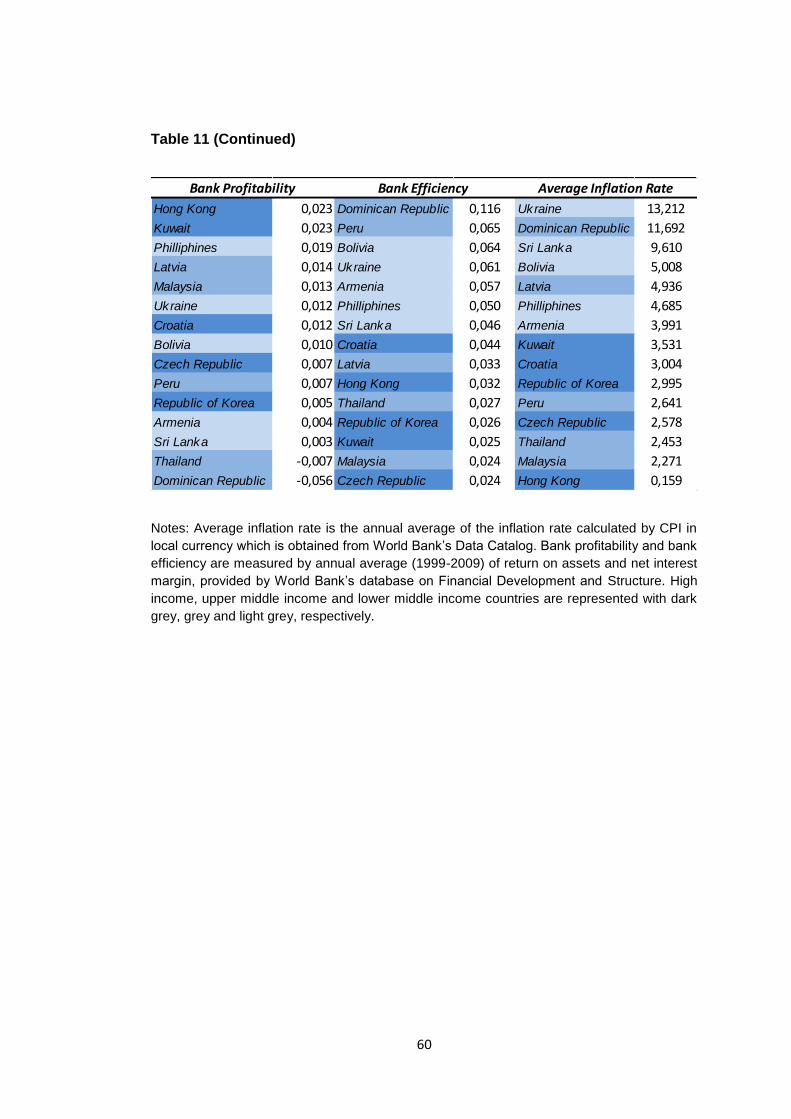
60

Table 11 (Continued)

Notes: Average inflation rate is the annual average of the inflation rate calculated by CPI in

local currency which is obtained from World Bank’s Data Catalog. Bank profitability and bank

efficiency are measured by annual average (1999-2009) of return on assets and net interest

margin, provided by World Bank’s database on Financial Development and Structure. High

income, upper middle income and lower middle income countries are represented with dark

grey, grey and light grey, respectively.

Hong Kong 0,023 Dominican Republic 0,116 Ukraine 13,212

Kuwait 0,023 Peru 0,065 Dominican Republic 11,692

Philliphines 0,019 Bolivia 0,064 Sri Lanka 9,610

Latvia 0,014 Ukraine 0,061 Bolivia 5,008

Malaysia 0,013 Armenia 0,057 Latvia 4,936

Ukraine 0,012 Philliphines 0,050 Philliphines 4,685

Croatia 0,012 Sri Lanka 0,046 Armenia 3,991

Bolivia 0,010 Croatia 0,044 Kuwait 3,531

Czech Republic 0,007 Latvia 0,033 Croatia 3,004

Peru 0,007 Hong Kong 0,032 Republic of Korea 2,995

Republic of Korea 0,005 Thailand 0,027 Peru 2,641

Armenia 0,004 Republic of Korea 0,026 Czech Republic 2,578

Sri Lanka 0,003 Kuwait 0,025 Thailand 2,453

Thailand -0,007 Malaysia 0,024 Malaysia 2,271

Dominican Republic -0,056 Czech Republic 0,024 Hong Kong 0,159

Bank Profitability Bank Efficiency Average Inflation Rate

61

APPENDIX C

TEZ FOTOKOPİ İZİN FORMU

ENSTİTÜ

Fen Bilimleri Enstitüsü

Sosyal Bilimler Enstitüsü

Uygulamalı Matematik Enstitüsü

Enformatik Enstitüsü

Deniz Bilimleri Enstitüsü

YAZARIN

Soyadı : DEĞER Adı : OSMAN Bölümü : İKTİSAT

TEZİN ADI (İngilizce) : A COMPARATIVE STUDY FOR NONLINEAR STRUCTURE OF THE INTEREST RATE PASS-THROUGH

TEZİN TÜRÜ : Yüksek Lisans Doktora

1. Tezimin tamamı dünya çapında erişime açılsın ve kaynak gösterilmek

şartıyla tezimin bir kısmı veya tamamının fotokopisi alınsın.

2. Tezimin tamamı yalnızca Orta Doğu Teknik Üniversitesi kullancılarının erişimine açılsın. (Bu seçenekle tezinizin fotokopisi ya da elektronik kopyası Kütüphane aracılığı ile ODTÜ dışına dağıtılmayacaktır.)

3. Tezim bir (1) yıl süreyle erişime kapalı olsun. (Bu seçenekle tezinizin

fotokopisi ya da elektronik kopyası Kütüphane aracılığı ile ODTÜ dışına dağıtılmayacaktır.)

Yazarın imzası ............................ Tarih .............................

X

X

X

62

Documents

A COMPARATIVE STUDY FOR NONLINEAR STRUCTURE OF THE