Steady-State

Nonisothermal Reactor Design

If you can't stand the heat. get out of the kitchen. Harry S Truman

Oveniew. Because most reactions we not carried out isothermally, we now focus our attention on heat effecrs in chemical reactors. The basic design equations, rate laws, and stoichiomctrjc relationships derived and used in Chapter 4 for isothermal reactor design are still valid for the design of nonisothermal reactors. The major difference lies in the method of evaluating the design equation when temperature varies along the length of a PFR or when heat is removed from a CSm. In Section 8.1, we show why we need the energy balance and how it will be used to solve: reactor design problems. h Sectior18.2, we develop the energy balance to a point where it can be applied to different types of reactors and then give the end result relating temperature and ~on\~ersion or reaction rate for the main types of reactors we have been studying. Section 8.3 shows how the energy balance is easily applied to design adiabatic reactors, while Section 8.4 deveIops the eneey balance on PFRsPBRs with heat exchange. In Section 8.5, the chemical equilibrium limitation on conver- sion is treated along with a strategy for staging reactors to overcome this limitadon. Sections 8.6 and 8.7 describe the: algorithm for a CSTR with heat effects and CSTRs with multiple steady states, respectively. Section 8.8 describes one of the most important tapics of the entire text. multiple reactions with heat effects, which is unique to this textbook. We close the chapter in Section 8.9 by considering hoth axial and radiat concenrrations and temperature gradients. The Prqf~ssiorrol AefEirnce Shdf R8.4 on the CD-ROM describes a typical nonisothermal industrial reactor and reac- tion, the SO2 oxidation, and gives many practical details.

472 Steady-State Nonisothermal Reactor Design CI

8.1 Rationale

To identify the additional information necessary to design nonisothermal tors, we consider the following example, in which a highly exothermic seas is carried out adiabatically in a plugflow reactor.

I Example 8-1 What Additional hiformation Is Required?

( Calculate the reactor volume necessary for 70% conversion.

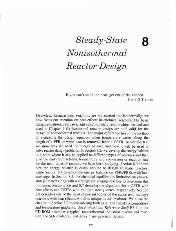
The reaction is exothermic and the reactor is operated adiabnticarly. As a resul temperature will increase with conversion down the length of the reactor.

- 1 1. Mole Balance (design equation):

2. Rate Law:

V - - I we know that k is a funct~on oh temperature, T.

3. Stoichiometry (liquid phase): u = uo

Combining Equations (Eg-1. I f , (ES-I.2). and (EX- 1.4) and canceling the er ing concentration. C,,, yields

v

Because T varies along the length of the reactor, k will also vary. which not the case for isothermal plug-flow reactors. Combining Equations (ES- and (E8-f -6) gives us

C, = C,(1 -X) (E8-

4. Combining:

I Sec. 8.2 The Energy Balance 473

Why we need the energy balance

, T,, = Entering

I Temperature

= Heat of React~on

i C,, = Heat Capacity

We see that we need another relationship relating X and Tor T and V to solve this equation. The mcrgy bnlance wiIl provide u.7 with this relationship. So we add another step to our algorithm. this step is the energy baIance.

5. Energy Balance: In this step. we will find the appropriate energy balance to relate temperature and convecsian or reaction rate. For example, if the reaction i s adiabatic. we will show the temperature-conversion relationship csn be wtitten in a form such as

We now have all the equations we need to solve for the conversion and tem- perature profiles.

I 8.2 The Energy Balance

I 8.2.1 First Law of Thermodynamics

We begin with the application of the first law of thermodynamics first to a closed system and then to an open system. A system is any bounded portion of the universe, moving or stationary, which is chosen for the application of the various thermodynamic equations. For a closed system, in which no ma2s crosses the system boundaries, the change in total energy of the system, d E , is equal to the heat flow to the system, 6Q, minus the work done by the sys- tem on the surroundings, 6W For a closed system, the energy balance is

d k = E Q - ~ W (8-1)

The 6's signify that SQ and FW are not exact differentials of a state function. The continuous-flow reactors we have been discussing are open systems

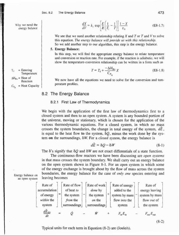
in that mass crosses the system bundary. We shalI carry out an energy halance on the open system shown in Figure 8-1. For an open system in which some of the energy exchange is brought about by the flow of mass across the system

Energy balance on boundaries, the energy balance for the case of on(v one species entering and an open system leaving becomes

(8-2)

Typical units for each term in Equation (8-2) are (Joulds).

7

Rate of accumulation

of energy within the

system j

- <

Rate of flow o f heat to

the system from the

surroundings

' -

- Rate of work

done by

the system on the

surroundings

+

- Rate o f energy

added to the system by mass

flow into the system

-

- - Rate o f

energy leaving system by mass

flow out of

the system A

Steady-State Nonisothermal Reactor Dasian Chap. 8

The s~aning point

Flow work and shaft wurk

Figure 8-1 Energy balance on a well-mixed open system: schematic.

We will assume the contents of the system volume are well mixed, an assumption that we could reIax but that would require a couple pages o f text to develop. and the end result would be the same! The unsteady-state energy balance for an open well-mixed system that has n species, each entering and leaving the system at their respective molar flow rates F, (moles of i per time) and with their respective energy Ei (joules per male of i ) , is

We will now discuss each of the terms in Quation (8-3).

8.2.2 Evaluating the Work Term

It is customary to separate the work rerm, W , into flow work and orher work, & . The term W,, often referred to as the shaft ~ ~ o r k , could be produced from such things as a stirrer in a CSTR or a turbine in a PFR. Flo~b uwrk is work that is necessary to get the mass into and our of the system. For example. when shear stresses are absent, we write

[Rate of flow work]

- where P i s the pressure (Pa) [ I Pa = 1 Newton/m2 = 1 kg d s 2 / m 2 ] and V, is the specific molar volume of species i (rn3/lmol of i).

Let's look at the units of the flow work term. which is

where Fi i s in molJs. P is Pa 1( 1 Pa = 1 Newton/m2), and ci is rn3/rnol.

- n ~ o l . Nenton , rn' F ; P . Y , [=I - - - - 1 - (Newtan*m).- = JouEesls = Watts s ,? mol S

Set, 8.2 The Energy Balance 475

We see that the units for flow work are consistent with the other terms in Equation (8-2), i.e., Its.

Jn most instances, the flow work term is combined with those terns in the energy balance that represent the energy exchange by mass flow across the system boundaries. Substjturing Equation (8-4) into (8-3) and grouping terms, we have

The energy Ei is the sum of the internal energy (U,), the kinetic enerm [u,2/2), the potential energy (gzi), and any other energies, such as electric or magnetic energy or light:

In almost all chemical reactor situations, the kinetic, potential, and "other" energy terms are negligible jn comparison with the entbalpy, heat transfer, and work terms, and hence will be omitted: that is.

Wc recall that the enfhalpy, H, (Jlrnol), is defined in terms of the internal energy U, (Jlmol). and the product PV, (1 %.m3/mol = 1 Jlmol):

Enthalpy Hi = ui + pQi (8-8)

Typical units of Hj are

J (Hi) = - Btu cal or - or - mol i Ib mol i mol i

Edthalpy carried into lor out of) the system can be expressed as the sum of the net internal energy carried into (or out of) the system by mass Aow plus the flow work:

F,H, = F,(u,+PV,) Combining Equations (8-5), (8-T), and (8-8). we can now write the energy bal- ance in the form

The energy of the system at any instant i n time, .k,!,, is the sum of the products of the number of moles of each species in the system multiplied by their respective energies. This term will be discussed in more detail when unsteady-state reactor operation i s considered in Chapter 9.

476 Steady-State Nonisothermal Reactor Design Ch

We shall let the subscript "0" represent the inlet conditions. Un scripted variables represent the conditions at the outlet of the chosen sy: volume.

F 4 , FH.,&~ I

-i'iT out In Section 8.1, we discussed that in order to solve reaction enginec

problems with heat effects, we needed to relate temperature, conversion,

rate of reaction. The energy balance as given in Equation (8-9) is the most venient starting point as we proceed to develop this relationship.

8.2.3 Overview of Energy Balances

What is the Plan? In the following pages we manipulate Equation (8-1 order to apply i t lo each of the reactor types we have been discussing, b PFR, PBR, and CSTR. The end result of the application of the energy bal to each type of reactor is shown in Table 8-1. The equations are used in St af the algorithm discussed in Example E8-1. The equations in Table 8-1 I

temperature to conversion and molar Row rates and to the system pararnr such as the overall heat-transfer coefficient and area. Ua, and correspor ambient temperature, T,. and the heat of reaction, AHRn-

End results of manipulating the

energy balance Sec- tions 8.1.1 to 8.4,

R 6, and 8.8.

F

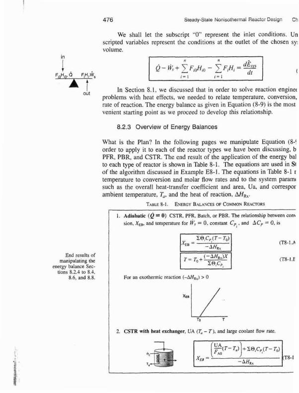
1. Adiabatic (L) = 0) CSTR, PFR, Batch, or PBR. The relationship between con\ sion. XEB, and temperature for W* = 0, constant Cp and ACp = 0, is

I '

ITS- I .A

(T8- 1 .E

For an exothermic reaction (-AHR,) > 0

70 T

2. CSTR with h a t exchanger, UA (T, - T ) , and large coolant flow rate.

Sec. 8.2 The Energy Balance 477

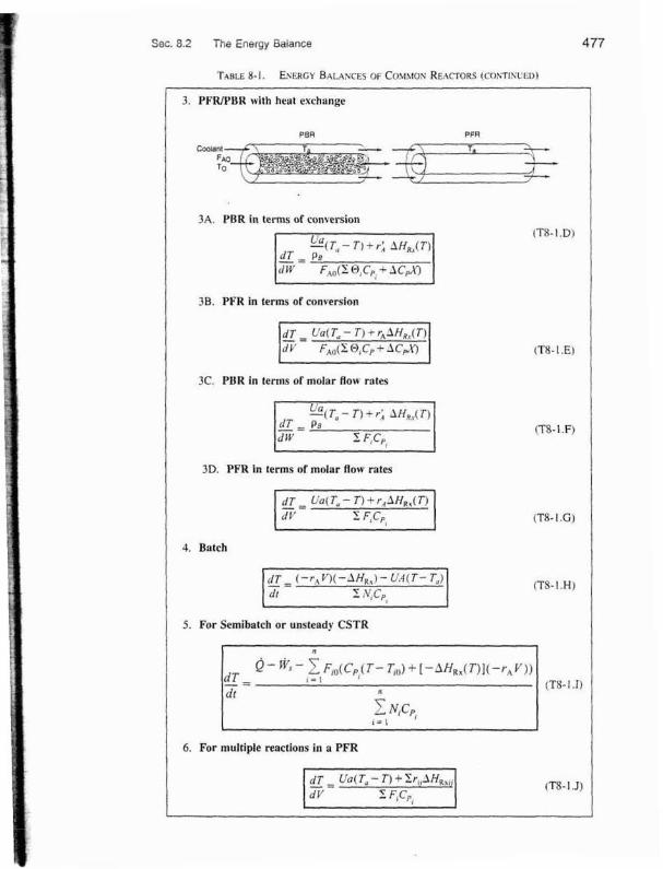
T.~BLE 8-1. E ~ E R G Y BALAXCES OF COMMON RE~ZCTORS (~Y)h'Tlhf El))

3A. PER in terms of conversion

38. PFR in terms of conversion

3C. PBR in terms of molar BOW rates

3D. PFR in terms of molar flaw rats

5 . For Semibatch or unsteady CSTR

6. For multiple teactlons in a PFR

dT - Ua( T, - T) + Xr,AH,,, (TS-l.J>

5 S,CrI

Adiabatic

478 Steadystate Nonisothermal Reactor Design Chap. El

TABLE 8-1. ENERGY BALANCES OF COMMON REACTORS (CO-D)

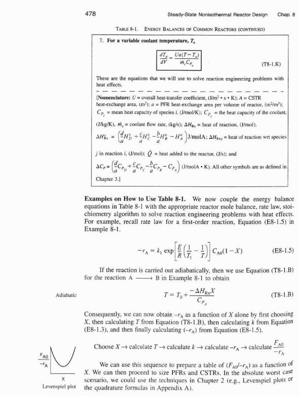
7. For a variable codant temperature, T,

(7-8-1.K)

These are the equations that we will use to sokve reaction engineering problems with heat effects. - - - - - - - + - - - - - - - - + - - - - -

[Nomenclaturr: I: = overall heat-transfer coefficient, (Jh? * s K): A = CSTR heat-exchange area, Im2). a = PFR heat-exchange area per volume of reactor. (m21m'l; CS = mean heat capacity of species i, (JlmolK): C p = the heat capacity of the coolant.

(JkJlkglK), ni, = coolant flour rate, tkgls); AH,, = hear of reactLon. Illmol):

b A H ; , = kD + f ~ ; - - H i - Jimol.4: AH..,, = heat of reaction w n species a a 1

j in reaction i. (JEmoll; Q = heat added to the reactor, (Jls); and

e C Up= -cPD+;cpc illrno1.A * K) AII other syrnhols are as dehned in

Chapter 3.1

Examples on How to Use Table 8-1. We now couple the energy balance equations in Table 8-1 with the appropriate reactor mole balance, rate law, smi- chiometry algorithm to solve reacdon engineering problems with heat effects. For example, recall rate law for a first-order reaction, Equation (Eg-1.5) in Example 8- 1 .

If the reaction is carried out adiabatically. then we use Equation IT&- I .B) for the reaction A d B in Example 8-1 to obtain

Consequently. we can now obtai~. -r, as a function of X done by first choosing X. then calculating T from Equation (TE- 1 .B). then calculating k from Equation (E8-1.3). and then finally calculating (-r,) from Equation (Eg-1.5).

F~~ Choose X 4 calculate T + calculate k + caIcuIate -rA + calculate - - ?'*

We can use this sequence lo prepare a table of (FA,+-r,) as a function of X . We can then proceed to size P F R ~ and CSTRs. In the absolute worst case

x scenario, we could use (he techniques in Chapter 2 (e.g.. Levenspiel plots or Lel'enspiel plot the quadrature formulas in Appendix A ) .

Sec. 8.2 The Energy Balance 479

Non-adiabatic PFR

Non-adiabatic CSTR

However, instead of using a Levenspiel plot, we will most likely use Polymath to solve our coupled differential energy and mole balance equations.

If there is cooling along the Iength of a PFR. we could then apply Qua- tion (T8-I .€) to this reaction to arrive at two coupled differential equations.

which are easily solved using an ODE solver such as Polymath. Similarly, for the case of the reaction A + B carried out in a CSTR. we

could use Polymath or MATLAB to solve two nonlinear equations in X and T. These two equations are combined moIe balance

and the application of Equation (T8-3 .C), which is rearranged in the form

From these three cases, (1) adiabatic PFR and CSTR, ( 2 ) PFR and PBR with heat effects. and (3) CSTR with heat effects, ane can see how one couples the energy balances and mole balances. In principle, one could simply use Table 8-1 to apply to different reactors and reaction systems without further discussion. However, understanding the derivation of these equations will greatly facilitate their proper application and evaluation to various reactors and reacfion systems. ConsequentIy, the following Sections 8.2. 8.3. 8.4, 8.6. and 8.8 will derive the equations given in Table 8-1.

why hother' Why bother to derive the equations in Table 8-1 ? Because I have found Here is why'! that students can a p l ~ l ~ these equations mucll more accurately to solve reaction

engineering problems with heat effects if they have gone through the deriva- tion to understand the assumptions and manipulations used in arriving at the equations in Table 8.1.

8.2.4 Dissecting the Steady-State Molar FEow Rates to Obtain the Heat of Reaction

To begin our journey, we start with the energy balance equation (8-9) and then proceed to finally arrive at the equations given i n Table 8-1 by first dissecting two terms.

480 Steady-State Noniscthermal Reactor Design Ch

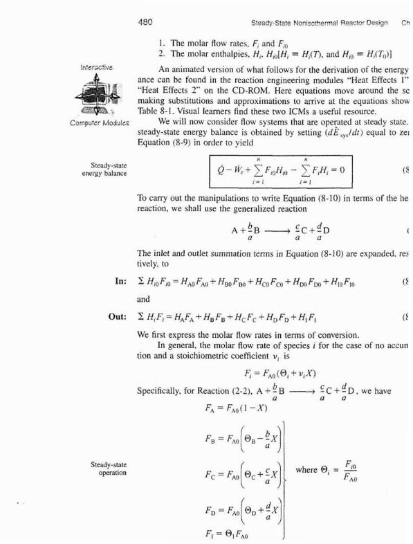
!. The molar Row sates. F, and FA, 2. The molar enthalpies, Hi. H,,,[H, = H,(n, and Ha HAT,)]

lnteractrvc An animated version of what foIlaws for the derivation of the energy ance can be found in the reaction engineering modules "Heat Effects 1" 'Weat Effects 2" on the CD-ROM. Here equations move around the sc making substitutions and approximations to arrive at the equations show

*~-'v.h Table 8-1. Visual learners find these two ICMS a useful resource. Cornpu:~: Modules We wiIl now consider Row systems that are operated at steady state.

steady-state energy balance is obtained by setting (dE',,,/dr) equaI to zel Equation (8-9) in order to yield

Steady -state energy balance

To carry out the manipulations to write Equation 18-10) in terms of the he reaction, we shall use the generalized reaction

The inlet and outIet summation tems in Equation (8- 10) are expanded. re: tively, to

In: Z HIo F,o = HAo FAo + ffBD FBo + Ha F*,, + Hm Fm + H10 FIO I F

and

We first express the molar Row rates in tems of conversion. In general. the molar Row rate of species i for the case of no accun

tion and a stoichiometric coefficient v, is

F, = FA, (Oi -+ v , X ) b d SpecificalIy, for Reaction (2-21, A -t - B + G C + - D , we have a a a

FA = FAD(I -X)

Steady-state operation

Sec. 8.2 The f nergy Balance 481

Heat of reaction at temperature T

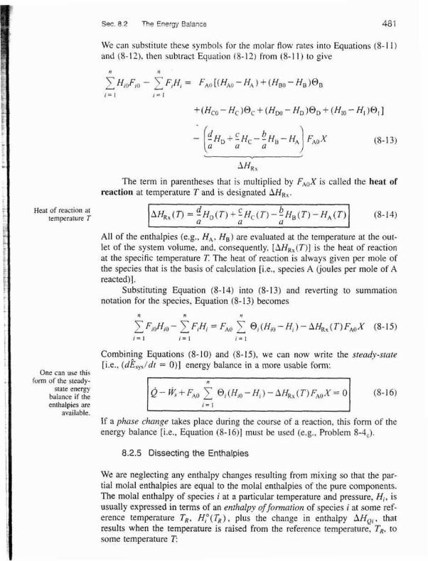
We can substitute thege symbolc for the molar flow rates into Equations (8-1 1 ) and (8-13). then subtract Equation (8-12) From (8-1 1 ) to give

The term in parentheses that is multiplied by FAOX is called the heat of reaction at temperature T and is designated AHR,.

All d the enthalpies (e.g., H A , HB) are evaluated at the temperature at the out- tet of the system volume, and, consequently. [AH,,(T)] is the heat of reaction at the specific temperature T. The heat of reaction is always given per mole of the species that is the basis of calculation [i.e., species A coules per mole of A reacted)].

Substituting Equation (8-14) into 18-13] and reverting to summation notation for the species. Equation (8- 13) becomes

Combining Equations (8-10) and (8-15), we can now write the steady-smte live., (dESy/d! = O)] energy balance in a more usable form:

One can use t h i ~ Form of the steady-

state energy balance if the enthalpres m

ava~lable. If a phase change takes place during the course of a reaction, this form of the energy balance [i.e., Equation (8-1611 must be used (e.g., Problem 5-4,).

8.2.5 Dissecting the Enthalpies

We are neglecting any enthalpy changes resulting from mixing so that the par- tial rnolal enthatpies are equaf to the mob1 enthalpies of the pure components. The molal enthalpy of species i at a particuIar temperature and pressure, Hi, is usually expressed in terms of an enthulpy offormarion of species i at some ref- erence temperature T,. H I 0 ( T R ) , plus the change in enthalpy AHQ,, that results when the temperature is raised from the reference temperature, TR. to some temperature T:

482 Steady-State Monisothermal Reactor Design Chap. B

Calculating the enthalpy when phase changes are involved

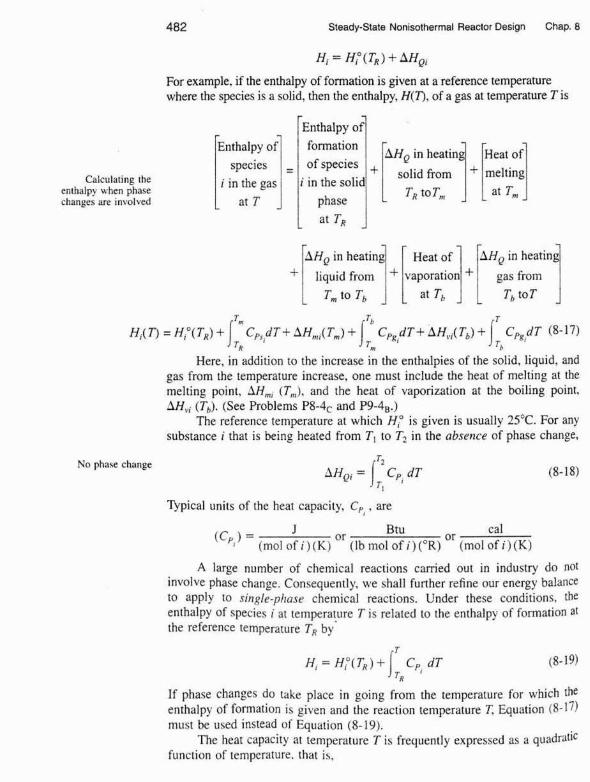
For example, if the enrhalpy of formation is given at a reference temperature where the species is a solid, then the enthalpy, H(?), of a gas a! tempemre T is

Here, in addition to the increase in the enthalpies of the solid, liquid. and gas from the temperature increase, one must include the heat of melting at the melting point, AH,, (T,,), and the heat of vaporizarion at the boiling point. AHvi (Tb). (See Problems P8-4c md P9-4B.)

The reference temperature at which HP is given is usuaIly 25OC. For any substance i that is being heated from TI to T2 in the absence of phase change,

Enthalpy of species in =

at T -

No phase change

Qpical units of the heat capacity, C,, , are

- - Enthalpy of formation ofspecies

i intbtbid at I;P -

or Btu or cal ( C p l ) = (moi of i ) (K) (Ib rnoi of i ) ( O R ) (mol of i ) (K)

AHQ in heating Heat of + 1 S:ptIp," ] + ",:I

A large number of chemical reactions carried out in industry do no1 involve phase change. Consequently, we shall further refine our energy balance to apply to single-phase chemical reactions. Under these conditions, the enthalpy of species i at temperature T is related to the enthalpy of formation at the reference temperature T, by-

H, = HP(T,) +J'p, d~ (8-19)

If phase changes do take place in going from the temperature for which the enthalpy of formatron i s given and the reaction temperature T, Equation 18-17] must be used insread of Equation (8-1 9).

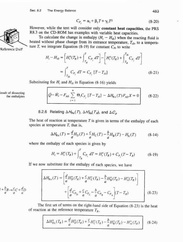
The heat capacity at temperature T i s frequently expressed as a quadratic function of temperature, that is.

S ~ C . 8.2 The Energy Balance 483

However, while the text will consider only constant heat capacities, the PRS R8.3 on the CD-ROM has examples with variable heat capacities.

To calculate the change in enthalpy (HI - H,v) when the reacting Ruid is heated without phase change from its entrance temperature, 4,, to a tempera- ture T, we integrare Equation (8-19) for constant C, to write

Reference Chef

Substituting for H, and in Equation (8-16) yieIds

Result of dissecttng the enthalpies

r = l

8.2.6 Relating A 4, ( T ) , A H",A TR), and A c,, The heat of reaction at temperature T is given in terms of the enthalpy of each species at temperature T, that is,

d b Af fk , (T) = -H~(T)+<H,(T)--H.(T)-H,(T)

a a a (8-14)

where the enthalpy of each species is given by

If we now substitute for the enthalpy of each species, we have

6 d 3 +-B+:c+-D a a a

The first set of terms on the right-hand side of Equation (8-23) is the beat of reaction at the reference temperature T,?

+ : H : ( T ~ ) - ~ H ; ( T , j -x : (T~) a

+ ;CP,,+

1 I" (8-23)

484 Steady-State Nonfsothermal Reactor Desiqn Cha

One can look up The enthalpies of formation of many compounds, HdO ITR) . are, usually ta the heats Ot lated at 25°C and ran readily be found in the Hnndbook of Chemisfq (

formation at TR. then calculate the Physics1 and simiSar handbooks. For other substances, the heat of combust

heat of reaction at (also available in these handbooks) can be used to determine the enthaipy this reference formation. The method of calculation is described in these handbooks. Fr temperature.

these values of the standard heat of formation, HP (7'') , we can calculate heat of reaction at the reference temperature T, from Equation (8-24).

The second term in brackets on the right-hand side of Equation (8-23 the overall change in the heat capacity per mole of A reacted. ACp,

Heat of reaction at tempraturc T

Note:

Combining Equations (8-25), (8-241, and 18-23) gives us

AHR, ( T ) = AH:, (TR) + ACp(T- TR)

Equation (8-26) gives the heat of reaction at any temperature Tin 1e1 of the heat of reaction at a reference temperature (usually 298 K) and the C term. Techniques for determining the heat of reaction at pressures above air spheric can be found in Chem2 For the reaction of hydrogen and nitroger 4WC, it was shown that the heat of reaction increased by only 670 as the pt sure was raised from 1 arm lo 200 atm!

Example 8-2 Heat of Reaction

Calculate the heat of reaction for the synthesis of ammonia from hydrogen nitrogen at ISVC in kcallrnol of N, reacted and also in Wrnol o f Hz reacted.

Solution N2 + 3H2 2NH3

Calculate the heat of reaction at the reference temperature using the heats of for tion of the reacting species obtained from Perry's r-landbook3 or the Handbaol Ckemisrry and Physics.

The heats of formation of the elements (HI, N,) are zero at 25°C.

I CRC Handbook of Chemistry and Phvsics (Boca Raton. Ra.: CRC Press, 2003). N. H. Chen, Process Reactor Design (Needham Heights, Mass.: Allyn and Bat 19831, p. 26.

3 31. P e q . D. W. Green, and D. Green. eds.. P~rry's Chemicai Engineers' Handbc 7th ed. (New York: McGraw-Hill, 1999).

Sec. 8.2 The Energy Balance

cal = 2 ( - 1 1.020) -

mol N? = -22,040 callmol N, reacted

AHz..(298 K) = -22.04 kcaltmol N, reacted

= -92.22 kJ/mol N, reacted

A ~ P = 2ChH3 - 3CpH2 - CsN2

= 2(8.92) - 3f6.992) - 6.984

= - 10.12 callmol N, reacted .K

E~othemrc reaction

= -23,3EO calJrnolN, = -23.31 kcatJrnol N?

= -23.3 kcal/rnol N, X 4.184 kJ/kcal

= -97.5 klfmol N2 (Recall: I kcal = 4.184 kJ)

The heat of reaction based on the moles of H2 reacted is

The minus sign indicates the reaction is exothermic. If the heat capacities are con- stant or ~f the mean heat capacities over the range 25 to 35O"C are readily available, the determination of AH,, at 150°C i c quite simple.

AH1, (423 K) = 5 3 mol Hz (-91.53 &) kJ = -32.51 - at423 K

rnol H2

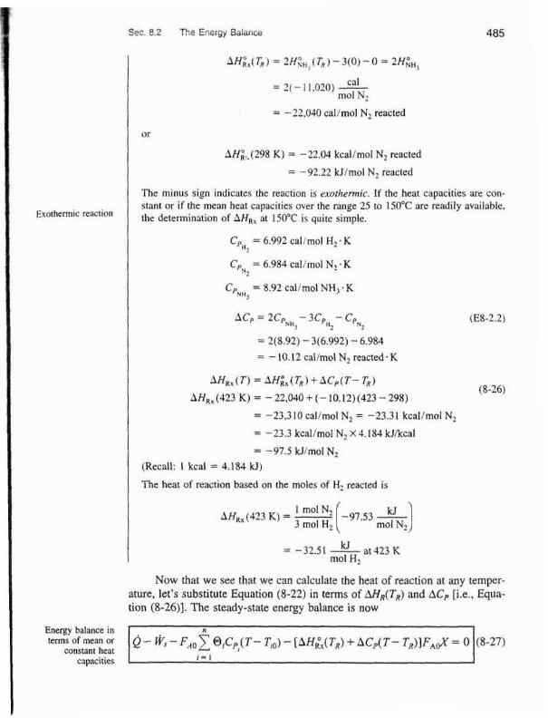
Now that we see that we can calculate the heat of reaction at any temper- ature, let's substitute Equation (8-22) in terns of AHR(TR) and AC, line., Equa- tion (8-2611. The steady-state energy balance is now

(8-27) Energy balance in terms of mean or

constant heat capacities . I = I

, n

Q- WS-FAOC @,Cp,(T- T id - [AHlx(Tf i ) + ACp(T- T,)]FAJ = 0

486 Steady-Stata Nonisothem1 Reactor Design Chap. I

Aom here on, for the sake of brevity we will let

unless otherwise specified. In most systems, the work term, w ~ , can be neglected (note the excep-

tion in the California Registration Exam Problem P8-5B at the end of this chapter) and the energy balance becomes

In almost all of the systems we will study, the reactants will be entering the system at the same temperature; therefore, T, = Tp

We can use Equation (8-28) to relate temperature and conversion and then proceed to evaluate the algorithm described in Example 8-1. However. unless the reaction i s carried out adiabatically, Equation (8-28) is still difficult to evaluare because in nooadiabatic reactors, the heat added ro or removed from the system varies along the length of the reactor. This problem does not occur in adiabatic reactors, which are frequently found in industry. Therefore, the adiabatic tubular reactor will be analyzed first.

8.3 Adiabatic Operation

Reactions in industry are frequently carried out adiabaticaIly with heating or cooling provided either upstream or downstream. Consequently, analyzing and sizing adiabatic reactors is an important task.

8.3.1 Adiabatic Energy Balance

In the previous section, we derived Equation (8-28). which relates conversion to temperature and the heat added to the reactor. Q. Let's stop a minute and consider a system wlth the special set of conditions of no work, Ws = 0 , adi- abatic operation i) = 0 , and then rearrange (8-27) into the form

For adiabatic operation. Example

8 I can now be solved' (8-29)

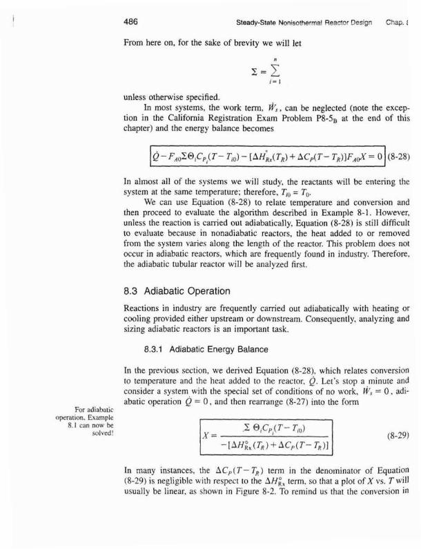
In many instances, the hC,(T-T,) term in the denominator of Equation (8-29) is negligible with respect to the AH;, term, so that a plot of X vs. Twill usually be linear, as shown in Figure 8-2. To remind us that the conversion i n

Sec. 8.3 Adiabatic Operation 487

Relationship between X and T

for udiahuric exothermic

reactions

Energy balance for adiabatic operation

of PER

this plot was obtained from the energy balance rather than the mole balance, it is given the subscript EB (i.e., XEs j in Figure 8-2. Equation (8-29) applies to a CSTR, PI%. PBR, and also to a batch (as will be shown in Chapter 9). For

= 0 and W, = 0, Equation (8-29) gives us the explicit relationship between X and T needed to be used in conjunction with the mole balance to solve Wac- tion engineering problems as discussed in Section 8.1.

CSTR PFR PBR Batch

XER

Figum 8-2 Adiabatic temperatuw-conversion relat~nn~hip.

6.3.2 Adiabatic Tubular Reactor

We can rearrange Equation (8-29) to solve for temperature as a function of conversion: that is

This equation will be coupled with the differential mole balance

to obtain the temperature, conversion. and concentration profifes along the length of the reactor. One way of analyzing this combination is to use Equation (8-30) to construct a table of T as a function of X. Once we have T as a func- tion of X, we can obtain k (T) as a function of X and hence -r, as a function of X alone. We could then use the procedures detailed in Chapter 2 ro size the

488 Steady-State Nonisotherrnal Reactor Des~gn Chal

different types of reactors; however. software packages such as Polymath z MATLAB can be used to solve the coupled energy balance and mole batar differential equations more easily.

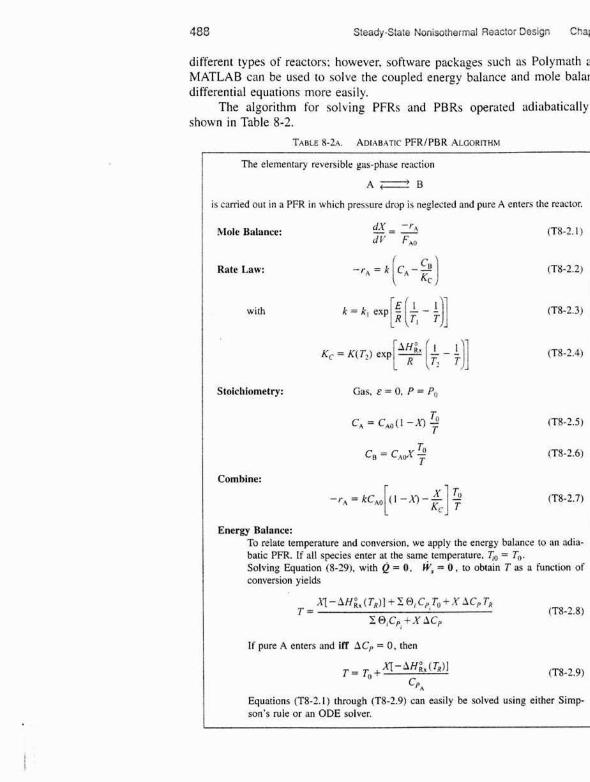
The algorithm far solving PFRs and PBRs operated adiabatically shown in Table 8-2.

TABLE 8-ZA. ADIABAT~C PFRIPBR ALGORITHM

with

A ~ B

is carried out in a PFR in which pressure drop i s neglected and pure A enten the reactor.

Mole Balance: d X - -r, fl8-2. I j ' F,,

(T8-2.2)

Gas, E = 0. P = Po

To c, = C*,II -x, - r To

CB = C A J 7

(T8-2.7)

Energy Balance: To relate temperature and conversion, we apply the energy balance to an adia- batic PFR. If all species enter at the same temperature, To = To. Solving Equation (8-29), with Q = O. W, = 0 , to obtain T as a function of conversion yields

X [ - i H i , ( T R ) ] + Z f ) , C p d T o L X . l C p T R (TR-2.8)

Z qc,, + X AC,

If pure A enters and IR AC, = 0, then

r= T,+ X [ - W , (&) I (T8-2.9) cpA

Sec. 8.3 Adiabatic Ooerar~on 489

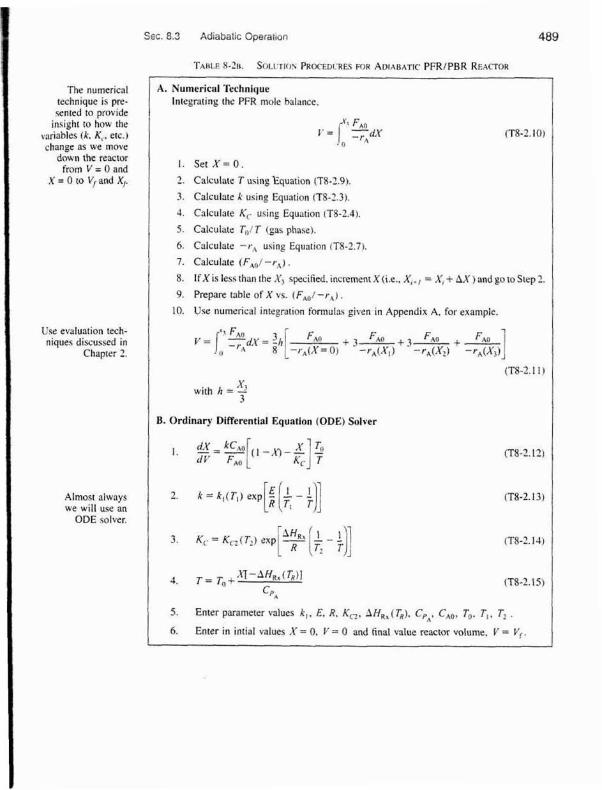
The numerrcal technique is pre- sented to provide

m i g h t to how the variables (k. K, , etc.) change as we move

down the reactor from V = 0 and

X = 0 to V, and XI.

TAHLF H-?H SOL^ Tft l l PROCEDCRE FOR ADIABATIC PER/PBR REACTOR

A. Numerical Technique

I Inletrating thc PFR mole balance.

Lree evaluation tech- niques discussed in

Chapter 2.

X with h = -!

3

I B. Ordinary Diffewntiai Equatinn (ODE) Solver

Almost always we will use an

ODE solver.

I. Set X = 0.

2 . Calculate T unng 'Equalion (T8-3.9)

3. Calculate 8 uslng Equation ITS-? 3).

4. CalcuIate K, uslng Equation (T8-2.4).

5 . Calculate T,,/ 7 (gas phaw).

6 Calculate -r , using Equation (T8-2 .7)

7. Calculate (F,,I - x , ) . 8. ITXIS less then the XI s~c i f ied . ~ncrementX(i.e.. X,., = X, t L Y )andgolo Step?,.

9. Prepare table of X VF (FA,/ -u, I . 10. Use numerical integration FormuIa~ pven in Appendix A. for example.

5 . Enter parameter values k, . E, R, Kc,, AH,, ( TR). CPAa C,,, To# T I , T? . 6. Enter in inrial vnlufi X = 0, Y = 0 and final value reactor volume, Y = Yr .