Noncommutative Gravity andQuantum Field Theory on

Noncommutative Curved Spacetimes

Dissertation zur Erlangung des

naturwissenschaftlichen Doktorgrades

der Bayerischen Julius-Maximilians-Universitat Wurzburg

vorgelegt von

Alexander Schenkel

aus Hardheim

Wurzburg 2011

Eingereicht am: 14. Juni 2011

bei der Fakultat fur Physik und Astronomie

1. Gutachter: Prof. Dr. Thorsten Ohl

2. Gutachter: Prof. Dr. Haye Hinrichsen

3. Gutachter: Prof. Dr. Peter Schupp (Jacobs University Bremen)

der Dissertation

1. Prufer: Prof. Dr. Thorsten Ohl

2. Prufer: Prof. Dr. Haye Hinrichsen

3. Prufer: Prof. Dr. Peter Schupp (Jacobs University Bremen)

4. Prufer: Prof. Dr. Thomas Trefzger

im Promotionskolloquium

Tag des Promotionskolloquiums: 24. Oktober 2011

Doktorurkunde ausgehandigt am:

Abstract

Over the past decades, noncommutative geometry has grown into an established field in pure mathematicsand theoretical physics. The discovery that noncommutative geometry emerges as a limit of quantum gravityand string theory has provided strong motivations to search for physics beyond the standard model of particlephysics and also beyond Einstein’s theory of general relativity within the realm of noncommutative geometries.A very fruitful approach in the latter direction is due to Julius Wess and his group, which combines deformationquantization (?-products) with quantum group methods. The resulting gravity theory does not only includenoncommutative effects of spacetime, but it is also invariant under a deformed Hopf algebra of diffeomorphisms,generalizing the principle of general covariance to the noncommutative setting.

The purpose of the first part of this thesis is to understand symmetry reduction in noncommutative gravity,which then allows us to find exact solutions of the noncommutative Einstein equations. These are importantinvestigations in order to capture the physical content of such theories and to make contact to applicationsin e.g. noncommutative cosmology and black hole physics. We propose an extension of the usual symmetryreduction procedure, which is frequently applied to the construction of exact solutions of Einstein’s field equations,to noncommutative gravity and show that this leads to preferred choices of noncommutative deformations ofa given symmetric system. We classify in the case of abelian Drinfel’d twists all consistent deformations ofspatially flat Friedmann-Robertson-Walker cosmologies and of the Schwarzschild black hole. The deformedsymmetry structure allows us to obtain exact solutions of the noncommutative Einstein equations in many of ourmodels, for which the noncommutative metric field coincides with the classical one.

In the second part we focus on quantum field theory on noncommutative curved spacetimes. We develop a newformalism by combining methods from the algebraic approach to quantum field theory with noncommutativedifferential geometry. The result is an algebra of observables for scalar quantum field theories on a large classof noncommutative curved spacetimes. A precise relation to the algebra of observables of the correspondingundeformed quantum field theory is established. We focus on explicit examples of deformed wave operators andfind that there can be noncommutative corrections even on the level of free field theories, which is not the case inthe simplest example of the Moyal-Weyl deformed Minkowski spacetime. The convergent deformation of simpletoy-models is investigated and it is shown that these quantum field theories have many new features compared toformal deformation quantization. In addition to the expected nonlocality, we obtain that the relation betweenthe deformed and the undeformed quantum field theory is affected in a nontrivial way, leading to an improvedbehavior of the noncommutative quantum field theory at short distances, i.e. in the ultraviolet.

In the third part we develop elements of a more powerful, albeit more abstract, mathematical approachto noncommutative gravity. The goal is to better understand global aspects of homomorphisms between andconnections on noncommutative vector bundles, which are fundamental objects in the mathematical descriptionof noncommutative gravity. We prove that all homomorphisms and connections of the deformed theory canbe obtained by applying a quantization isomorphism to undeformed homomorphisms and connections. Theextension of homomorphisms and connections to tensor products of modules is clarified, and as a consequencewe are able to add tensor fields of arbitrary type to the noncommutative gravity theory of Wess et al. As anontrivial application of the new mathematical formalism we extend our studies of exact noncommutative gravitysolutions to more general deformations.

i

Zusammenfassung

Uber die letzten Jahrzehnte hat sich die nichtkommutative Geometrie zu einem etablierten Teilgebiet derreinen Mathematik und der theoretischen Physik entwickelt. Die Entdeckung, dass gewisse Grenzfalle derQuantengravitation und Stringtheorie zu nichtkommutativer Geometrie fuhren, motivierte die Suche nach Physikjenseits des Standardmodells der Elementarteilchenphysik und der Einstein’schen allgemeinen Relativitatstheorieim Rahmen von nichtkommutativen Geometrien. Einen ergiebigen Ansatz zu letzteren Theorien, welcherDeformationsquantisierung (Sternprodukte) mit Methoden aus der Theorie der Quantengruppen kombiniert,wurde von der Gruppe um Julius Wess entwickelt. Die resultierende Gravitationstheorie ist nicht nur imstandenichtkommutative Effekte der Raumzeit zu beschreiben, sondern sie erfullt ebenfalls ein generalisiertes allge-meines Kovarianzprinzip, welches durch eine deformierte Hopf Algebra von Diffeomorphismen beschriebenwird.

Gegenstand des ersten Teils dieser Dissertation ist es Symmetriereduktion im Rahmen von nichtkommutativerGravitation zu verstehen und damit exakte Losungen der nichtkommutativen Einstein’schen Gleichungen zukonstruieren. Diese Untersuchungen sind von großer Bedeutung um den physikalischen Inhalt dieser Theorienherauszuarbeiten und den Kontakt zu Anwendungen, z.B. im Rahmen nichtkommutativer Kosmologie und Physikschwarzer Locher, herzustellen. Wir verallgemeinern die ubliche Methode der Symmetriereduktion, welcheeine Standardtechnik im Auffinden von Losungen der Einstein’schen Gleichungen ist, auf nichtkommutativeGravitation. Es wird gezeigt, dass unsere Methode zur nichtkommutativen Symmetriereduktion fur ein gegebenessymmetrisches System zu bevorzugten Deformationen fuhrt. Fur Abelsche Drinfel’d Twists klassifizieren wiralle konsistenten Deformationen von raumlich flachen Friedmann-Robertson-Walker Kosmologien und desSchwarzschild’schen schwarzen Loches. Aufgrund der deformierten Symmetriestruktur dieser Modelle konnenwir viele Beispiele von exakten Losungen der nichtkommutativen Einstein’schen Gleichungen finden, bei welchendas nichtkommutative Metrikfeld mit dem klassischen ubereinstimmt.

Im Fokus des zweiten Teils sind Quantenfeldtheorien auf nichtkommutativen gekrummten Raumzeiten. Dazuentwickeln wir einen neuen Formalismus, welcher algebraische Methoden der Quantenfeldtheorie mit nichtkom-mutativer Differentialgeometrie verknupft. Als Resultat unseres Ansatzes erhalten wir eine Observablenalgebrafur skalare Quantenfeldtheorien auf einer großen Klasse von nichtkommutativen gekrummten Raumzeiten. Eswird eine prazise Relation zwischen dieser Algebra und der Observablenalgebra der undeformierten Quan-tenfeldtheorie hergeleitet. Wir studieren ebenfalls explizite Beispiele von deformierten Wellenoperatoren undfinden, dass im Gegensatz zu dem einfachsten Modell des Moyal-Weyl deformierten Minkowski-Raumes, imAllgemeinen schon die Propagation freier Felder durch die nichtkommutative Geometrie beeinflusst wird. DieEffekte von konvergenten Deformationen werden in einfachen Spezialfallen untersucht, und wir beobachtenneue Aspekte in diesen Quantenfeldtheorien, welche sich in formalen Deformationen nicht zeigten. Zusatzlichzu der erwarteten Nichtlokalitat finden wir, dass sich die Beziehung zwischen der deformierten und der unde-formierten Quantenfeldtheorie nichttrivial verandert. Wir beweisen, dass dies zu einem verbesserten Verhaltender nichtkommutativen Theorie bei kurzen Abstanden, d.h. im Ultravioletten, fuhrt.

Im dritten Teil dieser Arbeit entwickeln wir Elemente eines leistungsfahigeren, jedoch abstrakteren, mathema-tischen Ansatzes zur Beschreibung der nichtkommutativen Gravitation. Das Hauptaugenmerk liegt auf globalenAspekten von Homomorphismen zwischen und Zusammenhangen auf nichtkommutativen Vektorbundeln, welchefundamentale Objekte in der mathematischen Beschreibung von nichtkommutativer Gravitation sind. Wirbeweisen, dass sich alle Homomorphismen und Zusammenhange der deformierten Theorie mittels eines Quan-tisierungsisomorphismus aus den undeformierten Homomorphismen und Zusammenhangen ableiten lassen. Eswird ebenfalls untersucht wie sich Homomorphismen und Zusammenhange auf Tensorprodukte von Modulninduzieren lassen. Das Verstandnis dieser Induktion erlaubt es uns die nichtkommutative Gravitationstheorie vonWess et al. um allgemeine Tensorfelder zu erweitern. Als eine nichttriviale Anwendung des neuen Formalismuserweitern wir unsere Studien zu exakten Losungen der nichtkommutativen Einstein’schen Gleichungen aufallgemeinere Klassen von Deformationen.

iii

Contents

Abstract i

Zusammenfassung iii

Introduction and Outline 1

Part I. Noncommutative Gravity 7

Chapter 1. Basics 91. The Hopf algebra of diffeomorphisms 92. Deformed diffeomorphisms 113. Noncommutative differential geometry 134. Quantum Lie algebras 155. ?-covariant derivatives, curvature and Einstein equations 16

Chapter 2. Symmetry reduction 191. Physical idea and the case of classical gravity 192. Deformed symmetry reduction: General considerations 203. Deformed symmetry reduction: Abelian Drinfel’d twists 214. Application to cosmology and the Schwarzschild black hole 23

Chapter 3. Exact solutions 291. Noncommutative gravity in the nice basis 292. Cosmological solutions 313. Black hole solutions 334. General statement on noncommutative gravity solutions 35

Chapter 4. Open problems 37

Part II. Quantum Field Theory on Noncommutative Curved Spacetimes 41

Chapter 5. Basics 431. Motivation 432. Some basics of Lorentzian geometry 433. Normally hyperbolic operators, Green’s operators and the solution space 444. Symplectic vector space and quantization 465. Algebraic states and representations 47

Chapter 6. Formalism 491. Notation 492. Condensed review of noncommutative differential geometry 493. Deformed action functional and wave operators 504. Deformed Green’s operators and the solution space 525. Symplectic R[[λ]]-module and quantization 556. Algebraic states and representations 57

Chapter 7. Properties 591. Symplectic isomorphism to a simplified formalism 592. Symplectic isomorphisms to commutative field theory 623. Consequences of the symplectic isomorphisms 64

v

vi CONTENTS

Chapter 8. Applications 671. Examples of deformed wave operators 672. Homothetic Killing deformations of FRW universes 713. Towards quantum field theory on the isotropically deformed de Sitter spacetime 784. A new noncommutative Euclidean quantum field theory 80

Chapter 9. Open problems 83

Part III. Noncommutative Vector Bundles, Homomorphisms and Connections 85

Chapter 10. Motivation and outline 87

Chapter 11. Preliminaries and notation 89

Chapter 12. Hopf algebras, twists and deformations 931. Twist deformation preliminaries 932. The quantization isomorphism DF 94

Chapter 13. Module homomorphisms 991. Quantization of endomorphisms 992. Quantization of homomorphisms 1023. Quasi-commutative algebras and bimodules 1034. Product module homomorphisms 106

Chapter 14. Bimodule connections 1111. Connections on right and left modules 1112. Quantization of connections 1123. Quasi-commutative algebras and bimodules 1144. Extension to product modules 1145. Extension to the dual module 116

Chapter 15. Curvature and torsion 121

Chapter 16. Noncommutative gravity solutions revisited 125

Chapter 17. Open problems and outlook 129

Conclusions 131

Appendix 135

Appendix A. Formal power series and the λ-adic topology 137

Appendix B. On the twist deformation of the algebra of field polynomials 145

Appendix C. O(λ2) Green’s operators for a noncommutative Minkowski spacetime 147

Appendix D. Diagrammatic proof of the associativity of ⊗R 149

Appendix E. Symbol index for Part III 151

Bibliography 153

Acknowledgements 157

List of publications 159

Lebenslauf 161

Erklarung 163

Introduction and Outline

Introduction

Physics has gone through a number of major conceptual changes in the early twentieth century. In particular,experiments in atomic physics revealed the quantum structure of nature at microscopic distances, and Einstein’stheory of general relativity provided us with a deeper understanding of space and time. Quantum mechanicswas later successfully combined with special relativity, leading to quantum field theory and eventually to thestandard model of particle physics. However, the understanding of how to combine general relativity with theconcepts of quantum mechanics is not yet complete, and quantum gravity remains a very active field of researchin mathematics, mathematical physics and also phenomenology. There are by now a number of serious candidatestowards a theory of quantum gravity with string theory, see e.g. [Pol05a, Pol05b], and loop quantum gravity,see e.g. [Rov07, Thi07], being the most prominent examples. These theories focus on different key aspects oneexpects of quantum gravity: String theory in particular on the unification of all fundamental interactions andloop quantum gravity on background independence. In addition to these two major frameworks, there are alsoother influential approaches like asymptotic safety [Reu98] and causal dynamical triangulations [AL98], whichhave already led to interesting insights into the quantum nature of spacetime and might be able to guide futurequantum gravity research.

Looking again at the two major conceptual changes in the early twentieth century one notices a puzzling feature:Classical mechanics is described in terms of geometry of the phasespace, which is a field in mathematics calledPoisson geometry. On the other hand, quantum mechanics is described in terms of noncommutative algebrasgenerated by position and momentum operators satisfying the canonical commutation relations [xi, pj ] = i~ δij 1.This noncommutativity and the resulting uncertainty relations are experimentally required and have been testedto a great precision. The formulation of general relativity is based on (pseudo-) Riemannian geometry, which is,similarly to Poisson geometry, a subfield of differential geometry. This means that, on the mathematical level,general relativity is comparable to classical mechanics, because both are formulated in a geometric language,which does not include any quantum effects. Since the transition from classical to quantum mechanics is atransition from geometry to noncommutative algebra, it is natural to ask the following question: Can we comecloser to a quantum theory of gravity by replacing the geometrical structures underlying general relativity bynoncommutative algebraic structures?

In mathematics, there are several examples of geometric structures which can be entirely described in algebraicterms. Based on a seminal theorem by Gel’fand and Naimark [GN94], we can equivalently describe topologicalspaces of a certain kind (locally compact Hausdorff spaces) by commutative C∗-algebras. In addition, Serre[Ser55] and Swan [Swa62] have shown that vector bundles are equivalent to finitely generated and projectivemodules over these algebras. The algebraic equivalent of Riemannian spin-geometry was found and investigatedintensively by Connes, see e.g. [Con94], and led to the definition of commutative spectral triples, consisting ofcommutative algebras, Hilbert spaces and Dirac operators. Note that all algebraic structures corresponding toclassical geometries are commutative. A natural generalization of classical geometry is thus obtained by allowingalso for noncommutative algebras. In this respect, a noncommutative topological space is a noncommutativeC∗-algebra, a noncommutative vector bundle is a finitely generated and projective module over this algebra and anoncommutative Riemannian spin-manifold is a noncommutative spectral triple.

Having understood the algebraic objects required to formulate noncommutative geometry there is still thequestion which noncommutative algebra or which noncommutative vector bundle we should choose in orderto appropriately describe a certain physical situation. Unfortunately, constructing a noncommutative theoryfrom scratch is in general very complicated, since, in contrast to classical geometry, we are often missingphysical intuition in the quantum case. An approach which turned out to be very fruitful in order to constructnoncommutative theories is quantization. In general terms, quantization is a set of rules (axioms) how toassociate to a commutative system a noncommutative one. A systematic approach to quantization, calleddeformation quantization, was developed in [BFF+78a, BFF+78b], see also Waldmann’s book [Wal07] for anintroduction. The starting point of this approach is a Poisson algebra, i.e. a commutative algebra A with a Poissonstructure ·, ·, which is quantized by introducing a new noncommutative product, the ?-product. This ?-productdepends on a deformation parameter, ~ in the case of quantum mechanics, and one demands that for ~→ 0 the?-commutator reduces to the Poisson bracket at leading order [a ?, b] = i~a, b+O(~2).

Motivated by the example of quantum mechanics we can start thinking about introducing a ?-product onspacetime in order to quantize it. In this case a natural deformation parameter is given by the Planck length,i.e. the scale where we expect quantum effects of geometry to become relevant. However, in contrast toclassical mechanics, we did not yet observe a Poisson structure on spacetime. Thus, it is not clear whichPoisson tensor should be used to construct the ?-product, or in other words, in which “direction” we shouldquantize. In order to understand the basic features of a deformation let us assume some Poisson tensor Θµν(x) onspacetime. The ?-commutator between coordinate functions at leading order in the deformation parameter λ reads

3

[xµ ?, xν ] = iλΘµν(x) +O(λ2). Thus, similar to the Planck cells in quantum mechanics, there will be minimalareas in spacetime due to the associated coordinate uncertainty relations. These minimal areas may dependon the position because of the x-dependence of the Poisson tensor. As it has been shown in [DFR94, DFR95],coordinate uncertainty relations are capable to limit the intrinsic resolution of spacetime, such that black holescan not be produced in the process of sharp localization. Moreover, the modified ultraviolet structure of spacetimeimmediately rises the hope to improve the mathematical description of physics, in particular the ultravioletdivergences in quantum field theory and curvature singularities in general relativity.

A possible explanation for the Poisson tensor and also the ?-product on spacetime is provided by stringtheory. There it has been found that open strings ending on D-branes in a B-field background Bµν are subjectto noncommutative geometry effects, see e.g. [CH99, Sch99, SW99] and references therein. These effectsmanifest themselves on the level of string theory in terms of modified scattering amplitudes. Taking the effectivefield theory limit, the B-field background still affects the physics on the brane, and leads to a noncommutativeYang-Mills theory thereon.

The relation to string theory and physical motivations led phenomenologists to study in great detail possibleeffects of noncommutative geometry in particle physics and cosmology. An overview of the work done in particlephysics can be obtained from [HPR01, HKM04, JMS+01, CJS+02, MPKT+05a, MPKT+05b, OR04, AOR06,AOR07] and for cosmology see e.g. [LMMP02, KYR05, ABJ+08, ABJ+09, KM11], and references therein.The model which was mostly used in these studies is the so-called canonical, or Moyal-Weyl, deformation, whereone assumes that [xµ ?, xν ] = i λΘµν is constant. In contrast to commutative theories, the noncommutativeones displayed a violation of Lorentz invariance in scattering amplitudes and preferred directions in the cosmicmicrowave background.

Assuming spacetime to be noncommutative, there is still the question of how to describe gravitation. Besidesusing noncommutative metric fields, see e.g. [A+05, ADMW06, KS07], there are also approaches based onhermitian metrics, see e.g. [CFF93, Cha01], or vielbeins, see e.g. [Cha04, AC09a, AC09b] and references therein.In addition to these rather conventional approaches, noncommutative geometry seems to provide a naturalmechanism for emergent gravity from noncommutative gauge theory and matrix models, see [Riv03, Yan09,Yan07, Ste07, Ste09, Ste10]. For reviews on different approaches to noncommutative gravity see [Sza06, MH08].

In our work we are guided by the approach of Wess and his group to noncommutative gravity [A+05,ADMW06]. In this theory the symmetries of general relativity, i.e. the diffeomorphisms, are considered as thefundamental object and are deformed. The generalization of the diffeomorphism symmetry is formulated in thelanguage of Hopf algebras, a mathematical object which is suitable for studying quantizations of Lie groupsor Lie algebras, see e.g. [Maj95, Kas95] for an introduction. A gravity theory is then constructed such that ittransforms covariantly under the deformed diffeomorphisms, which automatically results in noncommutativegeometry. Note that in noncommutative gravity we take into account quantum effects of the underlying manifold(λ-deformation), but a phasespace quantization of the metric field (~-deformation) is not yet included. Thus, weexpect noncommutative gravity to be a valid approximation of a full quantum gravity theory, which should bequantized in ~ and λ, in configurations where quantum fluctuations in the metric field are negligible. We canalso see noncommutative gravity in the following, more speculative, way. Since the ~-quantization of generalrelativity is plagued by serious difficulties, like the perturbative nonrenormalizability, the λ-deformation of theunderlying manifold might be the missing ingredient to improve the ~-quantization of the metric field.

In addition to noncommutative gravity, an interesting field of research is noncommutative quantum fieldtheory. The focus there is on quantum fields propagating on a fixed noncommutative spacetime and the resultingeffects. Due to the minimal areas present in a noncommutative spacetime, one expects improved mathematicalproperties of these quantum field theories in the ultraviolet, as well as interesting and distinct new physical effects.Noncommutative quantum field theory comes in many different varieties, in particular it was studied in a Euclideanand Lorentzian setting. In the Euclidean setting, remarkable results were obtained by Grosse and Wulkenhaar[GW05a, GW05b, GW04, GW09] and later also by Rivasseau and his group [RVTW06, GMRVT06, DGMR07]after a long series of investigations. It has been found that the Φ4-theory on the Moyal-Weyl space has interestingquantum properties, if one includes an additional quadratic term in the action. In particular, the theory isrenormalizible to all orders in the perturbation theory and the infamous Landau pole is not present. This isan improvement compared to the commutative Φ4-theory and rises hope for obtaining a rigorously definedinteracting 4-dimensional Euclidean quantum field theory by using noncommutative geometry methods. Eventhough there have been many attempts in this direction, see e.g. the review [BKSW10], similar results do not yetexist for noncommutative gauge theories. In the Lorentzian case, a considerable amount of research has beendone in order to understand perturbatively interacting quantum field theories. The model mostly used for thesestudies is the Moyal-Weyl deformed Minkowski spacetime. Different approaches to perturbation theory have

4

been investigated, see e.g. [Bah04, Zah06b], and there was for a long time the hope that the infamous UV/IR-mixing problem is not present in the Minkowski case. Recently, it was shown in [Bah10] and [Zah11b] thatthe UV/IR-mixing also occurs in the Hamiltonian and Yang-Feldman approach to noncommutative Minkowskiquantum field theory, even though the mechanism is different to the Euclidean case. These new results questionthe mathematical consistency of these approaches.

When going from the Minkowski spacetime to more general Lorentzian spacetimes, in particular curvedones, the number of approaches to noncommutative quantum field theory reduces considerably. An interestingformalism for deformed quantum field theory in the language of algebraic quantum field theory was developedby Dappiaggi, Lechner and Morfa-Morales [DLMM11], which is based on the concept of warped convolutionspreviously studied by Lechner and collaborators [GL07, GL08, BLS10]. In this approach an algebraic quantumfield theory, described by a net of observable algebras, is deformed by using methods similar to those developedby Rieffel [Rie93]. A different approach, focusing primarily on spectral geometry, was investigated by Paschkeand Verch [PV04]. In this thesis we will present a third approach to quantum field theory on noncommutativecurved spacetimes developed by myself and collaborators [OS10, SU10a, Sch11, Sch10], which is formulated inclose contact to the noncommutative gravity theory of Wess et al.

Outline of this thesis

This thesis consists of three main parts, focusing on different, but strongly connected, aspects of noncom-mutative geometry, gravity and quantum field theory. The purpose of this section is to provide a broad andnontechnical overview of the content of all three parts.

Part I. We are going to focus on physical aspects of the noncommutative gravity theory of Wess and hisgroup. Even though this theory was already developed in 2006, no results on its application to physical situations,for example cosmology or black hole physics, have been published until recently1. A detailed investigationof explicit models is an essential step to capture the physical content of the noncommutative gravity theory,and it is therefore a very important task for future developments in this field. This provides the motivationfor Part I. In Chapter 1 we review the noncommutative gravity theory under consideration [A+05, ADMW06].Since this theory makes use of mathematical methods of Hopf algebra theory, we first give a gentle introductionto Hopf algebras and their Drinfel’d twist deformations using explicit examples. Based on this we explainhow spacetime, as well as its differential geometry, can be deformed, leading to examples of noncommutativegeometries. We equip these noncommutative spacetimes with covariant derivatives, define their curvature andeventually a noncommutative version of Einstein’s equations, which are the underlying dynamical equationsof noncommutative gravity. After this introductory chapter we present in Chapter 2 our approach to symmetryreduction in noncommutative gravity [OS09b]. Remember that in classical general relativity, Friedmann-Robertson-Walker cosmologies and Schwarzschild black holes are characterized as configurations which areinvariant under a certain symmetry group (or Lie algebra). We generalize this definition to theories covariantunder deformed Hopf algebra symmetries, making use of the concept of infinitesimal deformed isometries,described by almost quantum Lie algebras. As an application we classify all possible abelian twist deformationsof spatially flat Friedmann-Robertson-Walker cosmologies and Schwarzschild black holes satisfying our axiomsof deformed symmetry reduction. The physical content of these models is briefly discussed and we find aparticularly interesting cosmological model, which is invariant under all classical rotations, and a deformed blackhole model, which is invariant under all classical black hole symmetries. In Chapter 3 we take the natural nextstep and construct exact solutions of the noncommutative Einstein equations within our models. The work wepresent was published in [OS09a] and appeared at the same time as the related articles by Schupp and Solodukhin[SS09] and Aschieri and Castellani [AC10], all of them focusing on different aspects of exact noncommutativegravity solutions. The main result of our work, which was also found in [SS07, SS09, AC10], is that the classicalmetric field satisfies the noncommutative Einstein equations exactly if the deformation is generated by sufficientlymany Killing vector fields. We show that this condition is fulfilled for most of our physically viable modelsof noncommutative cosmologies and black holes, thus leading to a large class of explicit physics examples. Inparticular, we show that also the isotropically deformed cosmological model solves the noncommutative Einsteinequations exactly in presence of a cosmological constant. Even though the metric field for these configurationsdoes not receive noncommutative corrections, the underlying manifold is quantized, leading to distinct physicaleffects which will be discussed. We conclude Part I by pointing out open problems in noncommutative gravity,which are the motivation for the developments described in Part III.

1 While working on this subject [OS09a] I became aware of earlier investigations by Schupp and Solodukhin on noncommutative blackholes, which were presented at conferences in 2007 [SS07] and later published in 2009 [SS09].

5

Part II. After the discussion of noncommutative background spacetimes in Part I we focus in Part II onnoncommutative quantum field theory. This is an important step towards extracting physical observables innoncommutative cosmology and black hole physics, for example the two-point correlation function yieldinginformation on the cosmological power spectrum or the Hawking radiation. Since noncommutative quantum fieldtheory is usually studied on the Moyal-Weyl deformed Minkowski spacetime, the analysis of our models requirestwo generalizations: Curved spacetimes and more general deformations. In other words, we have to developa formalism for quantum field theory on noncommutative curved spacetimes. In order to fix notation we firstreview in Chapter 5 the algebraic approach to quantum field theory on commutative curved spacetimes, whichhas turned out to be very fruitful, see e.g. [Wal94, BGP07, BF09]. We present our approach to quantum fieldtheory on noncommutative curved spacetimes [OS10] in Chapter 6, which combines algebraic quantum fieldtheory methods with noncommutative differential geometry. The result of this construction is a deformed algebraof observables for a scalar quantum field theory on a large class of deformed curved spacetimes. In Chapter 7 weexplore mathematical properties of our approach to quantum field theory on noncommutative curved spacetimesand in particular prove that each deformed quantum field theory can be mapped bijectively to an undeformedone [Sch10]. Chapter 8 is devoted to explicit examples of field and quantum field theories on noncommutativecurved spacetimes. We present examples of deformed wave operators on noncommutative Minkowski, de Sitter,Schwarzschild and anti-de Sitter spacetimes [SU10a]. We study in detail the explicit construction of a scalarquantum field theory on the isotropically deformed de Sitter spacetime, which is a nontrivial step towards physicalapplications in cosmology. As two more applications we focus on homothetic Killing deformations, yieldingsimple examples of exactly treatable models [Sch11], and we present a new perturbatively interacting quantumfield theory on a nonstandard deformed Euclidean space [SU10b], which shows remarkable similarities to therecently studied Horava-Lifshitz theories [Hor09] and has improved quantum properties. We close this part witha discussion of open problems in quantum field theory on noncommutative curved spacetimes.

Part III. In this part we focus on mathematical aspects of noncommutative geometry, which are basedon ongoing work with Paolo Aschieri [AS11]. The main motivation for these studies comes from the openproblems in noncommutative gravity and quantum field theory, which have shown that in particular metricfields and covariant derivatives are not yet completely understood in the noncommutative setting. To explainthe content of this part we remind the reader that in noncommutative geometry spacetime is described by anoncommutative algebra A and a vector bundle by a (finitely generated and projective) module V over A. Weconsider the situation where we have an action of a Hopf algebra H on A and V . This is a generalization ofthe setting we encounter in the noncommutative gravity theory of Part I, where the Hopf algebra H describesthe deformed diffeomorphisms, A the quantized functions on spacetime and V the quantized vector fields ordifferential forms. After fixing the notation in Chapter 11 and exploring some technical aspects of Drinfel’dtwist deformations in Chapter 12, we focus in Chapter 13 on module endomorphisms and homomorphisms. Weshow that every module endomorphism on V can be quantized to yield a module endomorphism on the twistquantized module V?, and even more that every module endomorphism on V? can be obtained in this way. Thus,there is an isomorphism between the quantized and unquantized module endomorphisms. We extend the resultsto homomorphisms between two modules. As a direct consequence, we find that the quantized dual module isisomorphic to the dual quantized module, meaning that there are no ambiguities in considering duals. We concludethis chapter by studying the extension of module homomorphisms to tensor products of modules, i.e. tensorfields. In Chapter 14 we investigate covariant derivatives (more precisely connections) in noncommutativegeometry. We consider connections on the module V satisfying the right Leibniz rule and provide a quantizationprescription to obtain connections on the deformed module V?. As in case of module homomorphisms, thisquantization map is an isomorphism, meaning that there is a one-to-one correspondence between the quantizedand unquantized connections. We show that for quasi-commutative algebras and bimodules2 we can extendconnections canonically to tensor products of modules. This is exactly the situation we face in noncommutativegravity when we want to extend the connection to tensor fields. The curvature and torsion of connections is studiedin Chapter 15. In Chapter 16 we apply our formalism to reinvestigate exact noncommutative gravity solutions. Incontrast to the investigations based on local coordinate patches in Chapter 3, we can now study solutions of thenoncommutative Einstein equations on a global level. In particular, we are able to extend the known results of[SS07, SS09, OS09a, AC10], see also Chapter 3, to a larger class of Drinfel’d twists. We conclude in Chapter 17by giving an outlook to further interesting applications that can be studied within our formalism and point outopen issues which remain to be solved for completing the construction of a noncommutative theory of gravity.

2 An algebra or bimodule is said to be quasi-commutative, if it is commutative up to the action of an R-matrix, see Chapter 13, Section3 for details.

Part I

Noncommutative Gravity

CHAPTER 1

Basics

In this chapter we give an introduction to the noncommutative gravity theory of Wess and his group [A+05,ADMW06].

1. The Hopf algebra of diffeomorphisms

LetM be an N -dimensional smooth manifold and let Ξ be the space of complex and smooth vector fields onM. Locally, there exists a basis ∂µ ∈ Ξ : µ = 1, . . . , N, such that every vector field v ∈ Ξ can be written asv = vµ(x)∂µ, where vµ(x) ∈ C∞(M), for all µ, are the coefficient functions. The space of vector fields can benaturally equipped with a Lie bracket, i.e. an antisymmetric C-bilinear map [·, ·] : Ξ× Ξ→ Ξ, which satisfiesthe Jacobi identity. Locally, the Lie bracket reads

[v, w] =(vµ(x)∂µw

ν(x)− wµ(x)∂µvν(x)

)∂ν , (1.1)

for all v, w ∈ Ξ. Thus,(Ξ, [·, ·]

)forms a complex Lie algebra.

The Lie algebra of vector fields(Ξ, [·, ·]

)plays an important role in differential geometry, namely it describes

the infinitesimal diffeomorphisms ofM. The action of(Ξ, [·, ·]

)on tensor fields is via the Lie derivative L. Note

that the Lie derivative and the Lie bracket are compatible, i.e. Lv Lw − Lw Lv = L[v,w], for all v, w ∈ Ξ.Let us point out two important operations one always has in mind when dealing with Lie algebras. These

observations are essential to understand the step how to go over from Lie algebras to Hopf algebras. We willdiscuss only the case of the Lie algebra

(Ξ, [·, ·]

), even though the same statements hold true for every Lie algebra(

g, [·, ·]). Firstly, note that for each vector field v ∈ Ξ, which we interpret as an infinitesimal diffeomorphism,

there is the inverse infinitesimal diffeomorphism vinv = −v ∈ Ξ. Secondly, having a product of representations,e.g. a tensor product τ ⊗ τ ′ of two tensor fields τ, τ ′, we can apply the Leibniz rule

Lv(τ ⊗ τ ′

)= Lv(τ)⊗ τ ′ + τ ⊗ Lv(τ ′) , (1.2)

for all v ∈ Ξ. Let us introduce also a third operation, which at the moment should be interpreted as a normalizationcondition. We define a map ε : Ξ→ C , v 7→ ε(v) = 0, which associates to all vector fields the number zero.

From the vector space Ξ we can always construct the free associative and unital algebra Afree. Elements ofAfree are finite sums of finite products of vector fields and the unit element 1. In order to encode informationon the Lie algebra structure of

(Ξ, [·, ·]

), we consider the ideal I generated by the elements v w − w v − [v, w],

for all v, w ∈ Ξ. The universal enveloping algebra of the Lie algebra(Ξ, [·, ·]

)is then defined to be the factor

algebra UΞ := Afree/I. Provided a representation, say tensor fields, of the Lie algebra(Ξ, [·, ·]

), we can extend

it to a left representation of UΞ by defining Lξ η = Lξ Lη , for all ξ, η ∈ UΞ, and L1 = id. The latter definitionallows us to interpret 1 as the trivial diffeomorphism.

We now implement the three additional operations we have for the Lie algebra into UΞ, starting with theLeibniz rule. Note that (1.2) gives us a prescription of how to transform products of representations. In a moreabstract language, not making use of the representation, the information of (1.2) can be encoded into a C-linearmap ∆ : UΞ→ UΞ⊗ UΞ, which on the generators reads

∆(v) = v ⊗ 1 + 1⊗ v , ∆(1) = 1⊗ 1 , (1.3)

for all v ∈ Ξ. We can extend this map to UΞ by demanding multiplicativity ∆(ξ η) = ∆(ξ) ∆(η), for allξ, η ∈ UΞ. The product on UΞ⊗ UΞ is given by (ξ ⊗ η) (ξ′ ⊗ η′) = ξ ξ′ ⊗ η η′. We can easily check that thisdefinition is consistent with the ideal I

∆(v w − w v) =(v ⊗ 1 + 1⊗ v

) (w ⊗ 1 + 1⊗ w

)− (v ↔ w)

= v w ⊗ 1 + v ⊗ w + w ⊗ v + 1⊗ v w − (v ↔ w)

= [v, w]⊗ 1 + 1⊗ [v, w] = ∆([v, w]) , (1.4)

for all v, w ∈ Ξ.Next, we implement the inverse operation vinv = −v ∈ Ξ. Again on a more abstract level, we are looking for

a C-linear map S : UΞ→ UΞ, which on the generators gives S(v) = −v, for all v ∈ Ξ, and S(1) = 1, since 1

9

10 1. BASICS

is the trivial diffeomorphism. Since we want to interpret S as a map giving the inverse of an element ξ ∈ UΞ, itis natural to extend it to UΞ as an antimultiplicative map, i.e. S(ξ η) = S(η)S(ξ), for all ξ, η ∈ UΞ. We cancheck that S defined like this is compatible with the ideal I

S(v w − w v) = S(v w)− S(w v) = S(w)S(v)− S(v)S(w)

= w v − v w = −[v, w] = S([v, w]) , (1.5)

for all v, w ∈ Ξ.It remains to extend the normalization ε to UΞ. We define the C-linear map ε : UΞ→ C on the generators by

ε(v) = 0, for all v ∈ Ξ, ε(1) = 1, and extend it to UΞ multiplicatively. This definition is consistent with theideal I

ε(v w − w v) = ε(v)ε(w)− ε(w)ε(v) = 0 = ε([v, w]) , (1.6)

for all v, w ∈ Ξ.Let us summarize this construction: Starting from the Lie algebra

(Ξ, [·, ·]

)we have constructed the universal

enveloping algebra UΞ. The intuitive notions of Leibniz rule, inverse and normalization, which we have on theLie algebra, were encoded on the level of UΞ in terms of C-linear maps ∆ : UΞ→ UΞ⊗ UΞ, S : UΞ→ UΞand ε : UΞ→ C. While ∆ and ε are multiplicative maps, the map S associated to inversion is antimultiplicative.The object which is of interest in the following is the quintuple H =

(UΞ, µ,∆, ε, S

), where µ denotes the

multiplication map in UΞ, which above was written simply as juxtaposition.The object H we have derived above from physical considerations is a structure which is well-known in

mathematics, namely a Hopf algebra. We refer to Part III for a mathematical definition of Hopf algebras and wewill continue in this section with our nontechnical treatment. Roughly speaking, a Hopf algebra is an algebratogether with three maps ∆, S and ε as above, which satisfy certain compatibility conditions. The map ∆ iscalled the coproduct, ε the counit and S the antipode. We shall now show that all these conditions hold true forour explicit example H =

(UΞ, µ,∆, ε, S

). This proves that we are indeed dealing with a Hopf algebra, which

will be of great importance later in this part. For H to be a Hopf algebra, the following three conditions have tohold true, for all ξ ∈ H , (

∆⊗ id)∆(ξ) =

(id⊗∆

)∆(ξ) , (1.7a)(

ε⊗ id)∆(ξ) = ξ =

(id⊗ ε

)∆(ξ) , (1.7b)

µ((S ⊗ id

)∆(ξ)

)= ε(ξ) 1 = µ

((id⊗ S

)∆(ξ)

), (1.7c)

where µ(ξ ⊗ η) = ξ η denotes the multiplication map. In order to check the conditions (1.7) we introduce aconvenient notation according to Sweedler: For any ξ ∈ H we write for the coproduct ∆(ξ) = ξ1 ⊗ ξ2 (sumunderstood). In this notation the conditions (1.7) read

ξ11⊗ ξ12

⊗ ξ2 = ξ1 ⊗ ξ21⊗ ξ22

, (1.8a)

ε(ξ1) ξ2 = ξ = ξ1 ε(ξ2) , (1.8b)

S(ξ1) ξ2 = ε(ξ) 1 = ξ1 S(ξ2) . (1.8c)

We first check these conditions on the level of the generators of H . For ξ = 1 the conditions trivially hold true.For ξ = u ∈ Ξ the left hand side of the first condition reads

u11⊗ u12

⊗ u2 = u1 ⊗ u2 ⊗ 1 + 11 ⊗ 12 ⊗ u = u⊗ 1⊗ 1 + 1⊗ u⊗ 1 + 1⊗ 1⊗ u . (1.9)

Evaluating the right hand side we obtain the same result, thus the first condition holds true. The second conditionalso holds for all generators u ∈ Ξ

ε(u1)u2 = ε(u) 1 + ε(1)u = u = u1 ε(u2) . (1.10)

Analogously, the third condition holds true

S(u1)u2 = S(u) 1 + S(1)u = −u+ u = 0 = ε(u) 1 = u1 S(u2) . (1.11)

In order prove that the conditions (1.7) are satisfied for generic elements of H it is sufficient to show that theyhold true for the product ξ η ∈ H , provided they hold for the individual ξ, η ∈ H . In the notation of (1.8) we

2. DEFORMED DIFFEOMORPHISMS 11

find

(ξ η)11⊗ (ξ η)12

⊗ (ξ η)2 = ξ11η11⊗ ξ12

η12⊗ ξ2 η2

=(ξ11⊗ ξ12

⊗ ξ2) (η11⊗ η12

⊗ η2

)=(ξ1 ⊗ ξ21

⊗ ξ22

) (η1 ⊗ η21

⊗ η22

)= ξ1 η1 ⊗ ξ21 η21 ⊗ ξ22 η22 = (ξ η)1 ⊗ (ξ η)21 ⊗ (ξ η)22 , (1.12a)

ε((ξ η)1) (ξ η)2 = ε(ξ1 η1) ξ2 η2 = ε(ξ1)ε(η1) ξ2 η2 = ε(ξ1) ξ2 ε(η1) η2 = ξ η , (1.12b)

and

S((ξ η)1) (ξ η)2 = S(ξ1 η1) ξ2 η2 = S(η1)S(ξ1) ξ2 η2 = ε(ξ) ε(η) 1 = ε(ξ η) 1 . (1.12c)

The right hand sides of the second and third condition (1.8) are shown analogously.The calculations performed above lead us to the following conclusion: We can associate to the Lie algebra

of diffeomorphisms(Ξ, [·, ·]

)a Hopf algebra H =

(UΞ, µ,∆, ε, S

). This Hopf algebra will be called the Hopf

algebra of diffeomorphisms. It includes information on the Leibniz rule (via the coproduct ∆) and on the inverseof a diffeomorphism (via the antipode S), and further has a normalization operation (via the counit ε). Vice versa,we can extract the Lie algebra

(Ξ, [·, ·]

)from H as follows: As a vector space, Ξ is isomorphic to the space of all

elements ξ ∈ H with coproduct

∆(ξ) = ξ ⊗ 1 + 1⊗ ξ . (1.13)

This vector space can be equipped with a Lie bracket by employing the commutator [ξ, η] = ξ η − η ξ, for allξ, η ∈ H . The resulting Lie algebra is isomorphic to

(Ξ, [·, ·]

).

2. Deformed diffeomorphisms

The Hopf algebra of diffeomorphisms H , as well as every Hopf algebra constructed from a Lie algebra alongthe lines presented above, has a particular feature: Taking the coopposite coproduct ∆cop(ξ) = ξ2 ⊗ ξ1 of ageneric element ξ ∈ H agrees with the coproduct itself, i.e. ∆ = ∆cop. This property is called cocommutativityand correspondingly the Hopf algebra H is called a cocommutative Hopf algebra. From the point of view ofHopf algebra theory this is a very special feature, which allows for generalizations. As we will point out in thissection, deformations of H will in general not be cocommutative anymore, but the coopposite coproduct willbe equal to the coproduct up to conjugation by an element R ∈ H ⊗ H , called the universal R-matrix. Thesame R-matrix will also appear in the commutation relations of two quantized functions, thus it encodes thenoncommutative structure of spacetime.

In order to deform H we have to introduce a deformation parameter λ, which in physical situations shall berelated to the Planck length. For our investigations we treat λ as a formal parameter, which can be seen as aperturbative approach. Nonperturbative, i.e. convergent, deformations are mathematically much more involvedand rare, such that for an investigation of the leading effects of our deformations using a formal approach seemsreasonable. As a drawback of the formal approach we have to extend the Hopf algebra H and the complexnumbers C by formal powers of λ, denoted by H[[λ]] and C[[λ]], respectively. Elements of H[[λ]] are given byformal power series ξ =

∑∞n=0 λ

n ξ(n), where ξ(n) ∈ H for all n ≥ 0. The zeroth order describes the classicalpart and higher orders describe possible corrections due to the deformation. The extension H[[λ]] is again a Hopfalgebra: The algebra structure is given by

ξ + η =

∞∑n=0

λn (ξ(n) + η(n)) , ξ η =

∞∑n=0

λn∑

m+k=n

ξ(m) η(k) , (1.14)

and the maps ∆, ε, S are defined componentwise, e.g.

∆(ξ) =

∞∑n=0

λn ∆(ξ(n)) . (1.15)

For mathematical details on formal power series, which we do not require for the present part, we refer to theAppendix A. In the remaining part the formal power series extension will be implicitly understood and we drop[[λ]] for notational convenience. This is a typical convention in the physics literature.

We now consider deformations of the Hopf algebra H . A Drinfel’d twist is an invertible element F ∈ H ⊗Hsatisfying the following two conditions

F12 (∆⊗ id)F = F23 (id⊗∆)F , (1.16a)

(ε⊗ id)F = 1 = (id⊗ ε)F , (1.16b)

12 1. BASICS

where F12 = F ⊗ 1 and F23 = 1⊗ F . We additionally demand that F = 1⊗ 1 +O(λ) in order to leave thezeroth order unchanged, which is reasonable since we interpret the zeroth order as the classical part. As an aside,this object is precisely a normalized 2-cocycle of the Hopf algebra H . From the physics perspective, the twoconditions (1.16) have a direct consequence for the noncommutative geometry we are going to construct later:The first condition ensures that the ?-product is associative, while the second leads to trivial ?-multiplications offunctions with the unit element. For later convenience we introduce the notationF = fα⊗fα andF−1 = fα⊗fα(sum over α understood) for the twist and its inverse. Note that fα, fα, fα, fα are elements in H .

Provided a twist F of the Hopf algebra H , there is a well-known theorem telling us that we can construct anew Hopf algebra HF :=

(UΞ, µ,∆F , ε, SF

)by deforming the coproduct and antipode according to

∆F (ξ) := F ∆(ξ)F−1 , SF (ξ) := χS(ξ)χ−1 , (1.17)

where χ := fα S(fα) and χ−1 = S(fα) fα. See for example Majid’s book [Maj95] for more details. Weintroduce the short notation ∆F (ξ) = ξ1F ⊗ ξ2F for the deformed coproduct.

Given the deformed Hopf algebra of diffeomorphisms HF the question arises if, and in which sense, it isdifferent to the Hopf algebra H we started with. For this remember that H is a cocommutative Hopf algebra,i.e. ∆cop = ∆. If we now consider the deformed coproduct ∆F we obtain for an arbitrary ξ ∈ HF

(∆F )cop(ξ) = F21 ∆cop(ξ)F−121 = F21 F−1 F ∆(ξ)F−1 F F−1

21 = F21 F−1 ∆F (ξ)F F−121 , (1.18)

where F21 = fα ⊗ fα and F−121 = fα ⊗ fα. Thus, the coopposite deformed coproduct is related to ∆F by

conjugation of the element R = F21F−1 ∈ HF ⊗HF , for all ξ ∈ HF ,

(∆F )cop(ξ) = R∆F (ξ)R−1 . (1.19)

This element is called a universal R-matrix. We introduce the convenient notation R = Rα ⊗ Rα andR−1 = Rα ⊗ Rα (sum over α understood) for the R-matrix and its inverse. The R-matrix satisfies in addition to(1.19) the following conditions

(∆F ⊗ id)R = R13R23 , (id⊗∆F )R = R13R12 , R21 = R−1 , (1.20)

where R12 = R⊗ 1, R23 = 1⊗R, R13 = Rα ⊗ 1⊗Rα and R21 = Rα ⊗Rα. A Hopf algebra together withan R-matrix satisfying (1.19) and (1.20) is called a triangular Hopf algebra. If the last property in (1.20) doesnot hold true, the Hopf algebra is called quasitriangular.

Note that while both HF and H are triangular Hopf algebras1, HF is in general not cocommutative (see theexample below). This means that HF is structurally different to the Hopf algebras generated by Lie algebras viathe universal enveloping algebra construction. As a consequence of this non-cocommutative behavior of HF , wewill obtain a noncommutative structure on the “spaces” the Hopf algebra acts on, e.g. the algebra of functions onM.

Let us present an explicit example of a particular deformed Hopf algebra of diffeomorphisms. We considerM = RN and denote by xµ, µ = 1, . . . , N , global coordinate functions onM. The derivatives ∂µ along xµ

provide a global basis of Ξ, such that every vector field v ∈ Ξ can be written as v = vµ(x)∂µ, with coefficientfunctions vµ ∈ C∞(RN ). In particular, ∂µ ∈ Ξ are globally defined vector fields for all µ = 1, . . . , N . Considerthe following element in UΞ⊗ UΞ

F = exp

(− iλ

2Θµν∂µ ⊗ ∂ν

), (1.21)

where Θµν is a constant and antisymmetric N ×N -matrix. A short calculation shows that F satisfies (1.16) andis invertible via

F−1 = exp

(iλ

2Θµν∂µ ⊗ ∂ν

). (1.22)

This means that F is a twist of H , the so-called Moyal-Weyl twist. The R-matrix of the deformed Hopf algebraHF reads

R = F21 F−1 = exp(iλΘµν∂µ ⊗ ∂ν

), (1.23)

and thus is nontrivial. The deformed coproduct of the vector fields ∂µ ∈ HF is undeformed, i.e.

∆F (∂µ) = ∆(∂µ) , (1.24)

1 The R-matrix of H is the trivial one 1⊗ 1.

3. NONCOMMUTATIVE DIFFERENTIAL GEOMETRY 13

since all ∂µ mutually commute. However, the deformed coproduct of the vector field v = Mνµx

µ∂ν ∈ Ξ, whereMνµ is a constant N ×N -matrix, reads

∆F (v) = v ⊗ 1 + 1⊗ v − iλ

2

(ΘρµMν

µ −ΘνµMρµ

)∂ρ ⊗ ∂ν . (1.25)

As it will become more clear in the following section, the Hopf algebra HF with F given by (1.21) describesthe diffeomorphism symmetries of the Moyal-Weyl space RNΘ , which is a noncommutative space. Equipping RN

with the Minkowski metric g = −dx1 ⊗ dx1 +∑Ni=2 dx

i ⊗ dxi and restricting the vector fields to Killing vectorfields K ⊆ Ξ, we obtain the deformed isometry Hopf algebra (UK, µ,∆F , ε, SF ) of the noncommutative space(RNΘ , g

). This Hopf algebra is also called the Θ-twisted Poincare Hopf algebra [CKNT04, CPT05].

3. Noncommutative differential geometry

In classical differential geometry, the Lie algebra of vector fields(Ξ, [·, ·]

)acts on tensor fields via the Lie

derivative L. As explained above, this action extends to a left action of H via Lξ η = Lξ Lη, for all ξ, η ∈ H ,and L1 = id. The aim of this section is to construct deformations of scalar, vector and tensor fields, whichtransform covariantly under the deformed Hopf algebra of diffeomorphisms HF . In order to simplify the notationwe will suppress the symbol L for the Lie derivative and simply write ξ(·) := Lξ(·), for all ξ ∈ UΞ.

Let us first focus on the simplest type of tensor field, namely the smooth and complex functions C∞(M). Thisspace can be equipped with an algebra structure by employing the pointwise multiplication (h k)(x) = h(x) k(x),for all h, k ∈ C∞(M). The algebra structure is covariant under the Hopf algebra H , since the followingproperties hold true, for all 1, h, k ∈ C∞(M) and ξ ∈ H ,

ξ(h k) = ξ1(h) ξ2(k) , ξ(1) = ε(ξ) 1 . (1.26)

In mathematical terms, this means that the algebra(C∞(M), ·

)equipped with the pointwise multiplication · is a

left H-module algebra.For nontrivial deformations F , the algebra

(C∞(M), ·

)fails to be covariant under HF (see the example

below). This failure is due to the nontrivial coproduct structure on HF . However, the algebra(C∞(M), ·

)can

be made covariant under HF , if we deform the product accordingly to F . This is a well-known and very generaltheorem in mathematics, see e.g. [Maj95] and Part III. In this section we explain this deformation using examples.For this consider the following deformed multiplication (?-product)

h ? k := fα(h) fα(k) , (1.27)

for all h, k ∈ C∞(M), where fα ⊗ fα = F−1 is the inverse twist. Due to the properties (1.16) of the twistthe ?-product is associative, i.e. (h ? k) ? l = h ? (k ? l), and fulfills 1 ? h = h = h ? 1. Thus,

(C∞(M), ?

)is

an associative algebra with unit, which however is in general noncommutative (see the example below). Thenoncommutativity is governed by the inverse R-matrix, since

h ? k = fα(h) fα(k) = fα(k) fα(h)

= (fβ fγ fα)(k) (fβ fγ fα)(h) = Rα(k) ? Rα(h) , (1.28)

for all h, k ∈ C∞(M). In the second line we have inserted the unit 1⊗ 1 = F−1 F .We now focus on the action of HF on the algebra

(C∞(M), ?

). Since HF and H are equal as algebras,

a left action of HF on the vector space C∞(M) is given by the usual Lie derivative. It remains to check if(C∞(M), ?

)is covariant under HF , i.e. if the deformed algebra is a left HF -module algebra. We obtain by an

explicit calculation

ξ(h ? k) = ξ(fα(h) fα(k)

)= (ξ1 f

α)(h) (ξ2 fα)(k)

= (fβ fγ ξ1 fα)(h) (fβ fγ ξ2 fα)(k) = ξ1F (h) ? ξ2F (k) , (1.29)

which means that the deformed coproduct ∆F is compatible with the ?-multiplication.This observation allows us to make the following interpretation of HF : Similarly as H describes the diffeo-

morphism symmetries of the classical manifoldM, the deformed Hopf algebraHF describes the diffeomorphismsymmetries of the noncommutative space

(C∞(M), ?

).

Before going on in the construction of a noncommutative differential geometry let us discuss an explicitexample. LetM = RN and F be the Moyal-Weyl twist (1.21). The corresponding ?-product then reads

h ? k = h eiλ2

←−∂µΘµν

−→∂ν k , (1.30)

14 1. BASICS

which is the usual Moyal-Weyl product. The algebra(C∞(RN ), ?

)transforms covariantly under the deformed

diffeomorphisms HF . Due to the nontrivial R-matrix of HF , the algebra(C∞(RN ), ?

)is noncommutative. In

particular, the commutation relations of the coordinate functions xµ ∈ C∞(RN ) read

[xµ ?, xν ] = xµ ? xν − xν ? xµ = iλΘµν 1 . (1.31)

We proceed in the construction of a noncommutative differential geometry. In classical differential geometryan object of central interest is the exterior algebra of differential forms

(Ω• :=

⊕Nn=0 Ωn,∧,d

), where Ωn is

the space of smooth and complex n-forms, ∧ : Ωn ⊗ Ωm → Ωm+n the wedge product and d : Ωn → Ωn+1

the exterior differential. Note that Ω0 = C∞(M). The exterior algebra is graded commutative, i.e. ω ∧ ω′ =

(−1)deg(ω)deg(ω′)ω′ ∧ ω, and it is covariant under H , since for all ω, ω′ ∈ Ω• and ξ ∈ H

ξ(ω ∧ ω′) = ξ1(ω) ∧ ξ2(ω′) . (1.32)

The differential d is equivariant under the action of H , for all ω ∈ Ω• and ξ ∈ H ,

ξ(dω) = d(ξ(ω)) , (1.33)

and satisfies the graded Leibniz rule, for all ω, ω′ ∈ Ω•,

d(ω ∧ ω′) = (dω) ∧ ω′ + (−1)deg(ω) ω ∧ (dω′) . (1.34)

Furthermore, the wedge product in Ω• provides us with a(C∞(M), ·

)-bimodule structure on the space of

n-forms. This is simply the pointwise multiplication of an n-form by a function from left or right, respectively.Due to the H-covariance of the exterior algebra, the bimodule structure is automatically covariant under H , i.e.

ξ(hω) = ξ1(h) ξ2(ω) , ξ(ω h) = ξ1(ω) ξ2(h) , (1.35)

for all h ∈ C∞(M), ω ∈ Ωn and ξ ∈ H .In order to render Ω• covariant under the deformed Hopf algebra of diffeomorphisms HF we introduce the

?-wedge product

ω ∧? ω′ := fα(ω) ∧ fα(ω′) , (1.36)

for all ω, ω′ ∈ Ω•. Due to (1.16) this product is associative and satisfies 1 ∧? ω = ω = ω ∧? 1, for all ω ∈ Ω•.It also defines a

(C∞(M), ?

)-bimodule structure on the space on n-forms. The covariance of these structures

under HF is easily checked and we obtain

ξ(ω ∧? ω′) = ξ1F (ω) ∧? ξ2F (ω′) , (1.37)

for all ω, ω′ ∈ Ω• and ξ ∈ HF . Analogously to the case of the deformed algebra of functions, the inverseR-matrix determines the deviation of

(Ω•,∧?

)from being graded commutative, more precisely we have

ω ∧? ω′ = (−1)deg(ω)deg(ω′)Rα(ω′) ∧? Rα(ω) , (1.38)

for all ω, ω′ ∈ Ω•.The deformed exterior algebra can be equipped with a differential. Due to the equivariance property (1.33) the

undeformed differential satisfies, for all ω, ω′ ∈ Ω•,

d(ω ∧? ω′) = (dω) ∧? ω′ + (−1)deg(ω)ω ∧? (dω′) , (1.39)

and thus is a differential on(Ω•,∧?

). We call

(Ω•,∧?,d

)the deformed differential calculus.

Another important geometric object we want to deform is the space of smooth and complex vector fields Ξ.This space has no algebra structure, but it is a bimodule over the algebra

(C∞(M), ·

). The left and right action

is given by the pointwise multiplication of a vector field by a function. The bimodule structure is H-covariant,i.e. for all h ∈ C∞(M), v ∈ Ξ and ξ ∈ H we have

ξ(h v) = ξ1(h) ξ2(v) , ξ(v h) = ξ1(v) ξ2(h) . (1.40)

Analogously to the case of n-forms above we introduce the deformed left and right multiplication

h ? v := fα(h) fα(v) , v ? h := fα(v) fα(h) , (1.41)

turning Ξ into a(C∞(M), ?

)-bimodule, which is covariant under HF .

Since in differential geometry vector fields and one-forms are dual to each other, we have a contraction〈·, ·〉 : Ξ× Ω1 → C∞(M). The contraction map Ω1 × Ξ→ C∞(M) will be denoted for notational simplicityby the same symbol. These contractions are H-covariant in the sense that

ξ(〈v, ω〉

)= 〈ξ1(v), ξ2(ω)〉 , (1.42)

4. QUANTUM LIE ALGEBRAS 15

for all v ∈ Ξ, ω ∈ Ω1 and ξ ∈ H . Furthermore, they satisfy the important property

〈h v, k ω l〉 = h 〈v k, ω〉 l , (1.43)

for all h, k, l ∈ C∞(M), v ∈ Ξ and ω ∈ Ω1. In order to make 〈·, ·〉 covariant under HF we use again the inversetwist and define

〈v, ω〉? := 〈fα(v), fα(ω)〉 , (1.44)

for all v ∈ Ξ and ω ∈ Ω1. It follows that the ?-contraction satisfies, for all h, k, l ∈ C∞(M), v ∈ Ξ and ω ∈ Ω1,

〈h ? v, k ? ω ? l〉? = h ? 〈v ? k, ω〉? ? l . (1.45)

The next step in the construction of the noncommutative differential geometry is to define deformed tensorfields. Consider the tensor algebra

(T ,⊗A

)generated by Ω1 and Ξ. The symbol ⊗A denotes the tensor product

over the algebra A =(C∞(M), ·

).2 The tensor product is by definition of the Lie derivative H-covariant, i.e.

ξ(τ ⊗A τ ′) = ξ1(τ)⊗A ξ2(τ ′) , (1.47)

for all τ, τ ′ ∈ T and ξ ∈ H . The desired HF -covariance of the tensor algebra is obtained by introducing thedeformed tensor product

τ ⊗A? τ ′ := fα(τ)⊗A fα(τ ′) , (1.48)

for all τ, τ ′ ∈ T . Let τ = τα ⊗A? τα ∈ T (sum over α understood) be a tensor field with τα, τα ∈ Ξ for all α(the same holds true for Ω1). We say that τ is symmetric/antisymmetric, if

τ = ± Rβ(τα)⊗A? Rβ(τα) . (1.49)

We can always evaluate the ?-tensor product and write the tensor field τ in terms of the usual tensor product τ =τα⊗A τα. Our definition of symmetry/antisymmetry in this basis reduces to the usual definition τ = ±τα⊗A τα.Thus, every classical symmetric/antisymmetric tensor field is also a deformed symmetric/antisymmetric tensorfield. As examples, deformed two-forms are antisymmetric tensor fields and the deformed metric field to bedefined later will be symmetric.

4. Quantum Lie algebras

In the sections above the focus was on the deformed Hopf algebra HF of diffeomorphisms. Since we requirethis concept later, we now show that we can associate to HF a quantum Lie algebra, similarly as we couldassociate to H the Lie algebra

(Ξ, [·, ·]

)of vector fields. We will be rather nontechnical in this section and refer

to [ADMW06] for details.In order to better understand the construction of the quantum Lie algebra, we first show that there is a Hopf

algebra H?, which is isomorphic to HF , but more convenient for later. Note that the undeformed Hopf algebraH acts on itself via the adjoint action

Adξ(η) := ξ1 η S(ξ2) . (1.50)

More precisely, the algebra(UΞ, µ

)is a left H-module algebra. Using the same twist deformation methods as

above, we deform this module algebra by introducing the ?-product

ξ ? η := Adfα(ξ) Adfα(η) , (1.51)

for all ξ, η ∈ UΞ. There is a remarkable relation between the algebras(UΞ, µ?

)and

(UΞ, µ

), namely they are

isomorphic. This has been observed first in [GM94] for this particular example and we later found out that ananalogous statement holds true for more general classes of algebras (see Chapter 12). The algebra isomorphismD :

(UΞ, µ?

)→(UΞ, µ

)is given by

D(ξ) := Adfα(ξ) fα , (1.52)

2 Remember that given two bimodules V,W over an algebra A, we can define their tensor product (over A) V ⊗A W as follows:Consider the free A-bimodule (V ×W )free generated by the Cartesian product V ×W and the A-subbimodule N generated by theelements

(v + v′, w)− (v, w)− (v′, w) , (v, w + w′)− (v, w)− (v, w′) , (1.46a)

(a v,w)− a (v, w) , (v a,w)− (v, aw) , (v, w a)− (v, w) a , (1.46b)

for all a ∈ A, v, v′ ∈ V andw,w′ ∈W . The tensor product V ⊗AW is defined by the quotientA-bimodule V ⊗AW := (V ×W )free/N .We denote by v ⊗A w the image of (v, w) ∈ V ×W under the natural map V ×W → V ⊗A W .

16 1. BASICS

for all ξ ∈ UΞ. For a proof we refer to Chapter 12. Due to this isomorphism we can pull-back the Hopfalgebra structure on HF to a Hopf algebra structure on

(UΞ, µ?

). We denote this Hopf algebra by H? =(

UΞ, µ?,∆?, ε?, S?), where the coproduct, counit and antipode are given by

∆? := (D−1 ⊗D−1) ∆F D , (1.53a)ε? := ε D , (1.53b)

S? := D−1 SF D . (1.53c)

This Hopf algebra is also triangular with R-matrix R? := (D−1 ⊗D−1)(R). Since H? and HF are isomorphicHopf algebras, any representation of HF is also a representation of H?. We denote the H?-action by the ?-Liederivative, for all ξ ∈ UΞ,

L?ξ := LD(ξ) . (1.54)

Let us now focus on the ?-coproduct ∆? of vector fields Ξ. One obtains the very compact expression

∆?(v) = v ⊗ 1 +D−1(Rα)⊗ Rα(v) , (1.55)

for all v ∈ Ξ. Acting with the ?-Lie derivative on, for example, a ?-tensor product of tensor fields we obtain

L?v(τ ⊗A? τ ′) = L?v(τ)⊗A? τ ′ + Rα(τ)⊗A? L?Rα(v)(τ′) , (1.56)

for all v ∈ Ξ and τ, τ ′ ∈ T . Note that this is up to the R-matrix the usual Leibniz rule for a vector field.With this observation we are able to construct a quantum Lie algebra in the sense of Woronowicz [Wor89].

Consider the vector fields Ξ equipped with the ?-Lie bracket [·, ·]? : Ξ× Ξ→ Ξ defined by

[v, w]? := [fα(v), fα(w)] , (1.57)

for all v, w ∈ Ξ. This bracket satisfies the deformed antisymmetry property

[v, w]? = −[Rα(w), Rα(v)]? , (1.58)

and the deformed Jacobi identity

[v, [w, z]?]? = [[v, w]?, z]? + [Rα(w), [Rα(v), z]?]? , (1.59)

for all v, w, z ∈ Ξ. Note that the following three properties hold true:

(1) Ξ generates H?

(2) [Ξ,Ξ]? ⊆ Ξ(3) ∆?(Ξ) ⊆ Ξ⊗ 1 + UΞ⊗ Ξ

Thus,(Ξ, [·, ·]?

)is a quantum Lie algebra corresponding to H?. This quantum Lie algebra acts on deformed

tensor fields via the ?-Lie derivative (1.54).Observe that the conditions a quantum Lie algebra has to satisfy are slight deformations of the Lie algebra

case. In particular, the deformed Lie bracket is allowed to be antisymmetric up to an R-matrix and the coproductis allowed to deviate in a controlled way from the usual Leibniz rule.

The quantum Lie algebra(Ξ, [·, ·]?

)should be interpreted as the infinitesimal deformed diffeomorphisms.

Covariance under(Ξ, [·, ·]?

)implies covariance under H?, since Ξ generates H?, and vice versa, which means

that we can now work completely on the level of quantum Lie algebras, without focusing on the Hopf algebraH?.

As a last remark, the Hopf algebra H? is more suitable for the definition of a quantum Lie algebra, since itsquantum Lie algebra is as a vector space simply Ξ. Using the isomorphism D, we obtain that the quantum Liealgebra ofHF is given as a vector space byD(Ξ) ⊆ UΞ, i.e. higher order products of vector fields. Working withΞ is simpler than working with D(Ξ), this is why we prefer H?. However, due to the isomorphism H? ' HFboth approaches are equivalent.

5. ?-covariant derivatives, curvature and Einstein equations

In this section we introduce covariant derivatives, torsion and curvature in the framework of the noncommuta-tive differential geometry presented in the section above. We will again suppress the symbol L for the (usual) Liederivative in order to compactify notation, i.e. ξ(·) = Lξ(·).

5. ?-COVARIANT DERIVATIVES, CURVATURE AND EINSTEIN EQUATIONS 17

A ?-covariant derivative O?v along a vector field v ∈ Ξ is a C-linear map O?v : Ξ → Ξ satisfying, for allv, w, z ∈ Ξ and h ∈ C∞(M),

O?v+wz = O?vz + O?wz , (1.60a)

O?h?vz = h ? O?vz , (1.60b)

O?v(h ? z) = L?v(h) ? z + Rα(h) ? O?Rα(v)z . (1.60c)

Given a ?-covariant derivative, its ?-torsion and ?-curvature are C-linear maps Tor? : Ξ ⊗ Ξ → Ξ andRiem? : Ξ⊗ Ξ⊗ Ξ→ Ξ defined by

Tor?(v, w) := O?vw − O?Rα(w)Rα(v)− [v, w]? , (1.61a)

Riem?(v, w, z) := O?vO?wz − O?Rα(w)O

?Rα(v)z − O

?[v,w]?

z , (1.61b)

for all v, w, z ∈ Ξ. These maps satisfy the antisymmetry properties

Tor?(v, w) = −Tor?(Rα(w), Rα(v)

), (1.62a)

Riem?(v, w, z) = −Riem?(Rα(w), Rα(v), z

), (1.62b)

and

Tor?(h ? v, k ? w) = h ? Tor?(v ? k,w) , (1.63a)

Riem?(h ? v, k ? w, l ? z) = h ? Riem?(v ? k,w ? l, z) , (1.63b)

for all v, w, z ∈ Ξ and h, k, l ∈ C∞(M).In order to construct the ?-Ricci tensor Ric? : Ξ ⊗ Ξ → C∞(M) we require a (local) basis ea : a =

1, . . . , N of Ξ. The dual basis θa : a = 1, . . . , N is defined by the conditions 〈ea, θb〉? = δba. The ?-Riccitensor is defined by the contraction

Ric?(v, w) :=

N∑a=1

〈θa,Riem?(ea, v, w)〉? , (1.64)

for all v, w ∈ Ξ. It is independent on the choice of basis and satisfies

Ric?(h ? v, k ? w) = h ? Ric?(v ? k,w) , (1.65)

for all h, k ∈ C∞(M) and v, w ∈ Ξ.Let us consider the example ofM = RN equipped with the Moyal-Weyl twist (1.21). In this case we have the

global basis ∂µ ∈ Ξ : µ = 1, . . . , N of vector fields Ξ. The ?-covariant derivative is completely specified bythe Christoffel symbols

O?∂µ∂ν = Γ?ρµν ? ∂ρ = Γ?ρµν ∂ρ , (1.66)

where in the last equality we have used that the twist acts trivially on all ∂ρ. In this basis the ?-torsion, ?-curvatureand ?-Ricci tensor reads

Tor?(∂µ, ∂ν) =(Γ?ρµν − Γ?ρνµ

)∂ρ , (1.67a)

Riem?(∂µ, ∂ν , ∂ρ) =(∂µΓ?σνρ − ∂νΓ?σµρ + Γ?τνρ ? Γ?σµτ − Γ?τµρ ? Γ?σντ

)∂σ , (1.67b)

Ric?(∂ν , ∂ρ) = ∂µΓ?µνρ − ∂νΓ?µµρ + Γ?τνρ ? Γ?µµτ − Γ?τµρ ? Γ?µντ , (1.67c)

where it was extensively used that the twist acts trivially on ∂ρ. For more general deformations, or a differentbasis of vector fields, these equations will be much more complicated, in the sense that R-matrices appear.

For a noncommutative gravity theory we require one more ingredient, a metric field g = gα ⊗A? gα ∈Ω1 ⊗A? Ω1. We demand g to be symmetric, real and nondegenerate. In particular, every classical metric fieldg ∈ Ω1 ⊗A Ω1 is also a metric field in the sense above. The ?-inverse metric g−1 = g−1α ⊗A? g−1

α ∈ Ξ⊗A? Ξis defined via the conditions

〈〈v, g〉?, g−1〉? = 〈v, gα〉? ? 〈gα, g−1β〉? ? g−1β = v , (1.68a)

〈〈ω, g−1〉?, g〉? = 〈ω, g−1β〉? ? 〈g−1β , gα〉? ? gα = ω , (1.68b)

for all v ∈ Ξ and ω ∈ Ω1.In Einstein’s theory of general relativity the metric field constitutes the dynamical degree of freedom and the

covariant derivative is fixed to be the Levi-Civita connection, i.e. the unique torsion-free and metric compatiblecovariant derivative. In noncommutative gravity, the existence and uniqueness of a ?-Levi-Civita connection,i.e. torsion-free ?-covariant derivative which is compatible with the metric tensor, is not yet completely understood.

18 1. BASICS

We will come back to this issue in Chapter 3, where we show that under certain conditions there is a unique?-Levi-Civita connection.

Continuing in the construction of the noncommutative Einstein equations, we define the ?-curvature scalar asthe contraction

R? := Ric?(g−1α, g−1α ) . (1.69)

The ?-Einstein tensor is given by the map G? : Ξ⊗ Ξ→ C∞(M),

G?(v, w) := Ric?(v, w)− 1

2g(v, w) ?R? , (1.70)

for all v, w ∈ Ξ, where g(v, w) := 〈v, 〈w, gα〉? ? gα〉?. It satisfies the property

G?(h ? v, k ? w) = h ? G?(v ? k,w) , (1.71)

for all h, k ∈ C∞(M) and v, w ∈ Ξ. The noncommutative Einstein equations for vacuum are thus

G?(v, w) = 0 , (1.72)

for all v, w ∈ Ξ. Provided a suitable stress-energy tensor T ? : Ξ ⊗ Ξ → C∞(M), one can also consider theEinstein equations coupled to matter

G?(v, w) = 8πGN T?(v, w) , (1.73)

for all v, w ∈ Ξ.Let us go back to the exampleM = RN deformed by the Moyal-Weyl twist (1.21). Using again that the twist

acts trivially on ∂ρ we can write for the metric field g = dxµ ⊗A dxνgµν = dxµ ⊗A? dxν ? gµν , since all ? dropout. The ?-inverse metric field g−1 = gµν ∂µ ⊗A ∂ν = gµν ? ∂µ ⊗A? ∂ν is determined by

gµν ? gνρ = δρµ , gµν ? gνρ = δµρ . (1.74)

It is simply the ?-inverse matrix of gµν . For this model there is a unique ?-Levi-Civita connection, see Chapter 3.The corresponding Christoffel symbols are given by

Γ?ρµν =1

2gρσ ? (∂µgνσ + ∂νgµσ − ∂σgµν) . (1.75)

Thus, the ?-Einstein tensor can be expressed completely in terms of the metric and the noncommutative Einsteinequations give rise to dynamical equations for the metric field.

CHAPTER 2

Symmetry reduction

In this chapter we present an approach to symmetry reduction in noncommutative gravity and its applicationto noncommutative cosmology and black hole physics. These results have been published in the research article[OS09b] and the proceedings article [Sch09].

1. Physical idea and the case of classical gravity

Consider a physical system consisting of a metric field g and a collection of matter fields (tensor fields)Φii∈I on a manifoldM. Since symmetry reduction in presence of gauge fields is more involved, we aregoing to neglect the effects of gauge fields in the present chapter. An example of such a system is inflationarycosmology, where one typically considers the metric field g and an inflaton field Φ on a suitable manifoldM(e.g.M = R4 orM = R× S3).

We assume that the dynamics of our system is described by Einstein’s equations Ric − 12gR = 8πGN T

and geometric differential equations for Φii∈I . Finding the most general solution of these highly nonlineardifferential equations turns out to be extremely hard and, even worse, practically impossible. In order to anyhowextract certain classes of exact solutions of the equations above, we have to make some physics input andassumptions. Symmetry reduction turns out to be a very powerful tool to do so.

We first explain the basic idea of symmetry reduction using the example of cosmology. From observations weknow that the universe, at large scales, is almost isotropic and homogeneous. So it seems to be reasonable to do azeroth order approximation and assume the universe to be exactly isotropic and homogeneous. The fluctuationswe observe for example in the cosmic microwave background (CMB) are then described in a second step byconsidering small perturbations on top of the highly symmetric background fields. If we demand the metric g andall matter fields Φii∈I to be isotropic and homogeneous, Einstein’s equations reduce to Friedmann’s equationsand also the differential equations for the matter fields simplify drastically. For certain models one can thenfind exact solutions, describing the evolution of a homogeneous and isotropic universe filled with homogeneousand isotropic matter. This model serves as a background for perturbative studies in cosmology, in particularphenomenological investigations on the CMB.

Let us now investigate symmetry reduction from the mathematical, i.e. differential geometric, perspective. LetM be a manifold, g a metric field and Φii∈I be a family of tensor fields. Let

(g, [·, ·]

)be a Lie subalgebra

of the Lie algebra of vector fields(Ξ, [·, ·]

). We implement the symmetries described by g on our system by

demanding the metric and all tensor fields to be invariant under g

Lg(g) = 0 , Lg(Φi) = 0 , ∀i ∈ I . (2.1)

As an aside, the symmetry condition (2.1) would be too strict for fields χ which also transform under someinfinitesimal gauge symmetry h. A reasonable definition in this case would be Lg(χ) ⊆ δh(χ), which means thatgauge equivalence classes should be invariant under g.

Demanding the symmetry condition (2.1) on the level of the fundamental fields the question arises if compositefields, like e.g. the curvature or the stress-energy tensor, are also invariant under g. This propagation of symmetriesis of great importance, since it ensures that the equations of motion are consistent when restricted to the symmetryreduced fields.

In classical differential geometry the propagation of symmetries is ensured by the coproduct of vector fields(the Leibniz rule) ∆(v) = v ⊗ 1 + 1⊗ v, for all v ∈ Ξ. Since all differential geometric constructions are definedsuch that they transform covariantly with respect to this coproduct, constructions out of g-invariant fields willbe g-invariant. Let us give some examples to clarify this: The tensor product of two invariant tensor fields τ, τ ′

is invariant, since Lv (τ ⊗A τ ′) = Lv(τ) ⊗A τ ′ + τ ⊗A Lv(τ ′) = 0, for all v ∈ g. Contractions of τ, τ ′ arealso invariant, since Lv(〈τ, τ ′〉) = 〈Lv(τ), τ ′〉+ 〈τ,Lv(τ ′)〉 = 0, for all v ∈ g. Furthermore, one easily showsthat the Levi-Civita connection, Riemann tensor, Ricci tensor, curvature scalar and finally the Einstein tensor isg-invariant in case the metric is.

19

20 2. SYMMETRY REDUCTION

2. Deformed symmetry reduction: General considerations

While in classical symmetry reduction one is interested in suitable Lie subalgebras(g, [·, ·]

)⊆(Ξ, [·, ·]

)of the Lie algebra of vector fields onM, in the noncommutative case Lie algebras are not expected to be anappropriate algebraic structure. This can be already seen on the level of the infinitesimal diffeomorphisms, whichare described by the quantum Lie algebra

(Ξ, [·, ·]?

)associated to the deformed Hopf algebra of diffeomorphisms

H?. So the basic ingredient for a deformed symmetry reduction should be given by a suitable subset g? ⊆ Ξcarrying some algebraic structures to be specified now. Since g? will be later interpreted as deformed infinitesimalisometries/symmetries of our models, there are natural conditions we would like to demand:

g? is a vector space (2.2a)

[g?, g?]? ⊆ g? (2.2b)

∆?(g?) ⊆ g? ⊗ 1 + UΞ⊗ g? (2.2c)

While the reason for demanding the first two conditions is obvious, we have to explain why we also demandthe third one. As explained in detail in the last section, an important feature of classical differential geometry isthat demanding symmetries for all fundamental fields, the symmetries propagate due to the Leibniz rule also tocomposite fields. Since the deformed Leibniz rule of vector fields, i.e. the coproduct ∆?, does not necessarilyhave this property, we have to make an assumption on ∆? in order to ensure that symmetries propagate tocomposite deformed fields. Let us explain why the third property leads to a propagation of the symmetry usingan example. Let τ, τ ′ ∈ T be two tensor fields, which are g?-invariant, i.e.

L?g?(τ) = L?g?(τ ′) = 0 . (2.3)

Due to the third condition (2.2c) we find for all v ∈ g?

L?v(τ ⊗A? τ ′) = L?v(τ)⊗A? τ ′ + Rα(τ)⊗A? L?Rα(v)(τ′) = 0 . (2.4)

The same holds true for all other deformed differential geometric operations, since they are covariant under H?.Note that the three conditions above are much weaker than demanding g? to be a quantum Lie algebra, since

this would require to replace (2.2c) by the stronger condition ∆?(g?) ⊆ g? ⊗ 1 + Ug? ⊗ g?. However, since(g?, [·, ·]?

)satisfies almost all conditions of a quantum Lie algebra we call it an almost quantum Lie subalgebra

of(Ξ, [·, ·]?

).

Provided an almost quantum Lie subalgebra(g?, [·, ·]?

)⊆(Ξ, [·, ·]?

), taking the deformation parameter

λ → 0 gives us a Lie subalgebra(g, [·, ·]

)⊆(Ξ, [·, ·]

)of the Lie algebra of vector fields onM. Thus, every

quantum symmetry gives rise to a classical Lie algebra in the commutative limit. For our purpose, the other wayaround is more interesting. Let

(g, [·, ·]

)⊆(Ξ, [·, ·]

)be a Lie subalgebra, which we interpret as the symmetries of

some classical physics model, e.g. translations and rotations in cosmology. It is important to find out under whichconditions we can construct an almost quantum Lie subalgebra

(g?, [·, ·]?

)such that λ → 0 yields

(g, [·, ·]

).

Note that this construction is always possible by making the choice g? = g + λΞ, which means that elementsof g? are given by v =

∑∞n=0 λ

n v(n), where v(0) ∈ g and v(n) ∈ Ξ for n > 0. Since in this case the higherorders in g? are∞-dimensional, demanding invariance under g? would provide too strong restrictions on tensorfields. This is why we consider this choice as unphysical and introduce the condition that g? has the samedimension as g. In the remaining part we will be even more restrictive and demand g? = g as vector spaces.The motivation for this choice is threefold: Firstly, it simplifies our explicit investigations in the next sections.Secondly, deforming only the action of a symmetry and not its underlying vector space structure fits into thedeformation philosophy of Chapter 1. Thirdly, this choice is mathematically distinguished from all other choicessince g? = g is a topologically free C[[λ]]-module (see Appendix A). With the choice g? = g the first condition(2.2a) is fulfilled. The second condition (2.2b) demands that the ?-Lie bracket closes on g. Taking a basisti ∈ g : i = 1, . . . ,dim(g) we thus require the existence of deformed structure constants f? kij ∈ C, such that

[ti, tj ]? = f? kij tk . (2.5)

By classical correspondence we know that f? kij = f kij +O(λ), where f k

ij are the structure constants of(g, [·, ·]

).

On the level of the generators ti, the third condition (2.2c) requires the existence of elements Q? ji ∈ UΞ, suchthat

∆?(ti) = ti ⊗ 1 +Q? ji ⊗ tj . (2.6)

It turns out that provided the most general twist F and the most general Lie subalgebra g the two conditions(2.5) and (2.6) are not satisfied. There are obstructions which give us relations between the deformation F andthe classical symmetries g which we want to quantize. This result is physically very attractive, since it meansthat if we want to deform g-symmetric systems, we can not use the most general twist, but the requirements

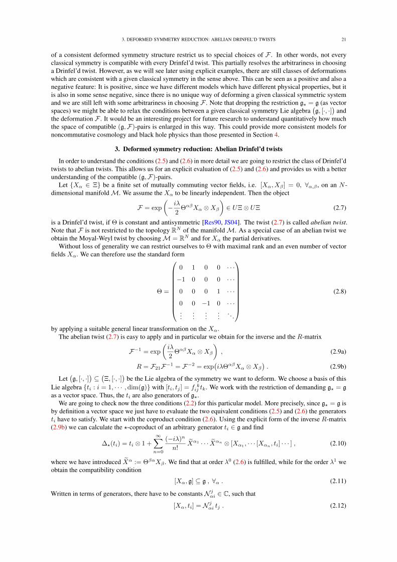
3. DEFORMED SYMMETRY REDUCTION: ABELIAN DRINFEL’D TWISTS 21

of a consistent deformed symmetry structure restrict us to special choices of F . In other words, not everyclassical symmetry is compatible with every Drinfel’d twist. This partially resolves the arbitrariness in choosinga Drinfel’d twist. However, as we will see later using explicit examples, there are still classes of deformationswhich are consistent with a given classical symmetry in the sense above. This can be seen as a positive and also anegative feature: It is positive, since we have different models which have different physical properties, but itis also in some sense negative, since there is no unique way of deforming a given classical symmetric systemand we are still left with some arbitrariness in choosing F . Note that dropping the restriction g? = g (as vectorspaces) we might be able to relax the conditions between a given classical symmetry Lie algebra

(g, [·, ·]

)and

the deformation F . It would be an interesting project for future research to understand quantitatively how muchthe space of compatible (g,F)-pairs is enlarged in this way. This could provide more consistent models fornoncommutative cosmology and black hole physics than those presented in Section 4.

3. Deformed symmetry reduction: Abelian Drinfel’d twists

In order to understand the conditions (2.5) and (2.6) in more detail we are going to restrict the class of Drinfel’dtwists to abelian twists. This allows us for an explicit evaluation of (2.5) and (2.6) and provides us with a betterunderstanding of the compatible (g,F)-pairs.

Let Xα ∈ Ξ be a finite set of mutually commuting vector fields, i.e. [Xα, Xβ ] = 0, ∀α,β , on an N -dimensional manifoldM. We assume the Xα to be linearly independent. Then the object

F = exp

(− iλ

2ΘαβXα ⊗Xβ

)∈ UΞ⊗ UΞ (2.7)

is a Drinfel’d twist, if Θ is constant and antisymmetric [Res90, JS04]. The twist (2.7) is called abelian twist.Note that F is not restricted to the topology RN of the manifoldM. As a special case of an abelian twist weobtain the Moyal-Weyl twist by choosingM = RN and for Xα the partial derivatives.

Without loss of generality we can restrict ourselves to Θ with maximal rank and an even number of vectorfields Xα. We can therefore use the standard form

Θ =

0 1 0 0 · · ·

−1 0 0 0 · · ·

0 0 0 1 · · ·

0 0 −1 0 · · ·...

......

.... . .

(2.8)

by applying a suitable general linear transformation on the Xα.The abelian twist (2.7) is easy to apply and in particular we obtain for the inverse and the R-matrix

F−1 = exp

(iλ

2ΘαβXα ⊗Xβ

), (2.9a)

R = F21F−1 = F−2 = exp(iλΘαβXα ⊗Xβ

). (2.9b)

Let(g, [·, ·]

)⊆(Ξ, [·, ·]

)be the Lie algebra of the symmetry we want to deform. We choose a basis of this

Lie algebra ti : i = 1, · · · ,dim(g) with [ti, tj ] = f kij tk. We work with the restriction of demanding g? = g

as a vector space. Thus, the ti are also generators of g?.We are going to check now the three conditions (2.2) for this particular model. More precisely, since g? = g is

by definition a vector space we just have to evaluate the two equivalent conditions (2.5) and (2.6) the generatorsti have to satisfy. We start with the coproduct condition (2.6). Using the explicit form of the inverse R-matrix(2.9b) we can calculate the ?-coproduct of an arbitrary generator ti ∈ g and find

∆?(ti) = ti ⊗ 1 +

∞∑n=0

(−iλ)n

n!Xα1 · · · Xαn ⊗ [Xα1

, · · · [Xαn , ti] · · · ] , (2.10)

where we have introduced Xα := ΘβαXβ . We find that at order λ0 (2.6) is fulfilled, while for the order λ1 weobtain the compatibility condition

[Xα, g] ⊆ g , ∀α . (2.11)

Written in terms of generators, there have to be constants N jαi ∈ C, such that

[Xα, ti] = N jαi tj . (2.12)

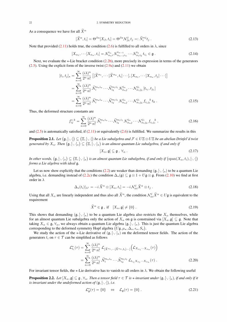
22 2. SYMMETRY REDUCTION

As a consequence we have for all Xα

[Xα, ti] = Θβα[Xβ , ti] = ΘβαN jβi tj =: Nαj

i tj . (2.13)

Note that provided (2.11) holds true, the condition (2.6) is fulfilled to all orders in λ, since

[Xα1 , · · · [Xαn , ti] = N inαniN in−1

αn−1in· · · N i1

α1i2ti1 ∈ g . (2.14)

Next, we evaluate the ?-Lie bracket condition (2.2b), more precisely its expression in terms of the generators(2.5). Using the explicit form of the inverse twist (2.9a) and (2.11) we obtain

[ti, tj ]? =

∞∑n=0

(iλ)n

2n n!

[[Xα1 , · · · [Xαn , ti] · · · ], [Xα1

, · · · [Xαn , tj ] · · · ]]

=

∞∑n=0

(iλ)n

2n n!Nαnini · · · Nα1i1

i2N jnαnj· · · N j1

α1j2[ti1 , tj1 ]

=

∞∑n=0

(iλ)n

2n n!Nαnini · · · Nα1i1

i2N jnαnj· · · N j1

α1j2f ki1j1 tk . (2.15)

Thus, the deformed structure constants are

f? kij =

∞∑n=0

(iλ)n

2n n!Nαnini · · · Nα1i1

i2N jnαnj· · · N j1

α1j2f ki1j1 , (2.16)

and (2.5) is automatically satisfied, if (2.11) or equivalently (2.6) is fulfilled. We summarize the results in this

Proposition 2.1. Let(g, [·, ·]

)⊆(Ξ, [·, ·]

)be a Lie subalgebra and F ∈ UΞ⊗UΞ be an abelian Drinfel’d twist

generated by Xα. Then(g, [·, ·]?

)⊆(Ξ, [·, ·]?

)is an almost quantum Lie subalgebra, if and only if

[Xα, g] ⊆ g , ∀α . (2.17)

In other words,(g, [·, ·]?

)⊆(Ξ, [·, ·]?

)is an almost quantum Lie subalgebra, if and only if

(span(Xα, ti), [·, ·]

)forms a Lie algebra with ideal g.

Let us now show explicitly that the conditions (2.2) are weaker than demanding (g, [·, ·]?) to be a quantum Liealgebra, i.e. demanding instead of (2.2c) the condition ∆?(g) ⊆ g⊗ 1 + Ug⊗ g. From (2.10) we find at firstorder in λ

∆?(ti)|λ1 = −i Xα ⊗ [Xα, ti] = −iN jαiX

α ⊗ tj . (2.18)

Using that all Xα are linearly independent and thus also all Xα, the condition N jαiX

α ∈ Ug is equivalent to therequirement

Xα ∈ g , if [Xα, g] 6= 0 . (2.19)

This shows that demanding (g, [·, ·]?) to be a quantum Lie algebra also restricts the Xα themselves, whilefor an almost quantum Lie subalgebra only the action of Xα on g is constrained via [Xa, g] ⊆ g. Note thattaking Xα ∈ g, ∀α, we always obtain a quantum Lie algebra (g, [·, ·]?). This is just the quantum Lie algebracorresponding to the deformed symmetry Hopf algebra

(Ug, µ?,∆?, ε?, S?

).

We study the action of the ?-Lie derivative of (g, [·, ·]?) on the deformed tensor fields. The action of thegenerators ti on τ ∈ T can be simplified as follows

L?ti(τ) =

∞∑n=0

(iλ)n

2n n!L[Xα1 ,···[Xαn ,ti]··· ]

(LXα1

···Xαn (τ))

=

∞∑n=0

(iλ)n

2n n!Nαnini · · · Nα1i1

i2Lti1Xα1

···Xαn (τ) . (2.20)

For invariant tensor fields, the ?-Lie derivative has to vanish to all orders in λ. We obtain the following useful

Proposition 2.2. Let [Xα, g] ⊆ g ,∀α. Then a tensor field τ ∈ T is ?-invariant under (g, [·, ·]?), if and only if itis invariant under the undeformed action of (g, [·, ·]), i.e.

L?g(τ) = 0 ⇔ Lg(τ) = 0 . (2.21)

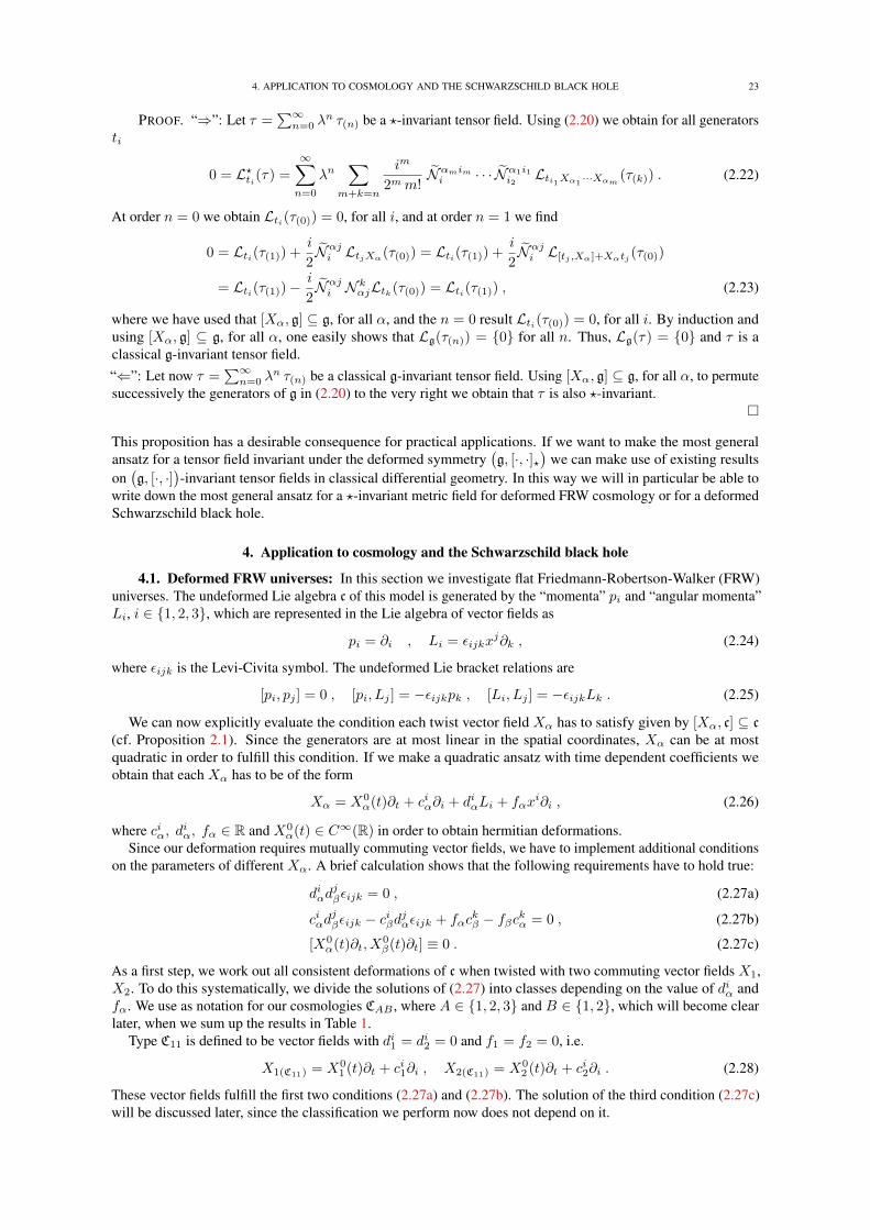
4. APPLICATION TO COSMOLOGY AND THE SCHWARZSCHILD BLACK HOLE 23

PROOF. “⇒”: Let τ =∑∞n=0 λ

n τ(n) be a ?-invariant tensor field. Using (2.20) we obtain for all generatorsti

0 = L?ti(τ) =

∞∑n=0

λn∑

m+k=n

im

2mm!Nαmimi · · · Nα1i1

i2Lti1Xα1 ···Xαm (τ(k)) . (2.22)

At order n = 0 we obtain Lti(τ(0)) = 0, for all i, and at order n = 1 we find

0 = Lti(τ(1)) +i

2Nαji LtjXα(τ(0)) = Lti(τ(1)) +

i

2Nαji L[tj ,Xα]+Xαtj (τ(0))

= Lti(τ(1))−i

2Nαji N

kαjLtk(τ(0)) = Lti(τ(1)) , (2.23)

where we have used that [Xα, g] ⊆ g, for all α, and the n = 0 result Lti(τ(0)) = 0, for all i. By induction andusing [Xα, g] ⊆ g, for all α, one easily shows that Lg(τ(n)) = 0 for all n. Thus, Lg(τ) = 0 and τ is aclassical g-invariant tensor field.“⇐”: Let now τ =

∑∞n=0 λ

n τ(n) be a classical g-invariant tensor field. Using [Xα, g] ⊆ g, for all α, to permutesuccessively the generators of g in (2.20) to the very right we obtain that τ is also ?-invariant.

This proposition has a desirable consequence for practical applications. If we want to make the most generalansatz for a tensor field invariant under the deformed symmetry

(g, [·, ·]?

)we can make use of existing results

on(g, [·, ·]

)-invariant tensor fields in classical differential geometry. In this way we will in particular be able to

write down the most general ansatz for a ?-invariant metric field for deformed FRW cosmology or for a deformedSchwarzschild black hole.

4. Application to cosmology and the Schwarzschild black hole

4.1. Deformed FRW universes: In this section we investigate flat Friedmann-Robertson-Walker (FRW)universes. The undeformed Lie algebra c of this model is generated by the “momenta” pi and “angular momenta”Li, i ∈ 1, 2, 3, which are represented in the Lie algebra of vector fields as

pi = ∂i , Li = εijkxj∂k , (2.24)

where εijk is the Levi-Civita symbol. The undeformed Lie bracket relations are

[pi, pj ] = 0 , [pi, Lj ] = −εijkpk , [Li, Lj ] = −εijkLk . (2.25)

We can now explicitly evaluate the condition each twist vector field Xα has to satisfy given by [Xα, c] ⊆ c(cf. Proposition 2.1). Since the generators are at most linear in the spatial coordinates, Xα can be at mostquadratic in order to fulfill this condition. If we make a quadratic ansatz with time dependent coefficients weobtain that each Xα has to be of the form

Xα = X0α(t)∂t + ciα∂i + diαLi + fαx

i∂i , (2.26)

where ciα, diα, fα ∈ R and X0

α(t) ∈ C∞(R) in order to obtain hermitian deformations.Since our deformation requires mutually commuting vector fields, we have to implement additional conditions

on the parameters of different Xα. A brief calculation shows that the following requirements have to hold true:

diαdjβεijk = 0 , (2.27a)

ciαdjβεijk − c

iβd

jαεijk + fαc

kβ − fβckα = 0 , (2.27b)

[X0α(t)∂t, X

0β(t)∂t] ≡ 0 . (2.27c)

As a first step, we work out all consistent deformations of c when twisted with two commuting vector fields X1,X2. To do this systematically, we divide the solutions of (2.27) into classes depending on the value of diα andfα. We use as notation for our cosmologies CAB , where A ∈ 1, 2, 3 and B ∈ 1, 2, which will become clearlater, when we sum up the results in Table 1.

Type C11 is defined to be vector fields with di1 = di2 = 0 and f1 = f2 = 0, i.e.

X1(C11) = X01 (t)∂t + ci1∂i , X2(C11) = X0

2 (t)∂t + ci2∂i . (2.28)

These vector fields fulfill the first two conditions (2.27a) and (2.27b). The solution of the third condition (2.27c)will be discussed later, since the classification we perform now does not depend on it.

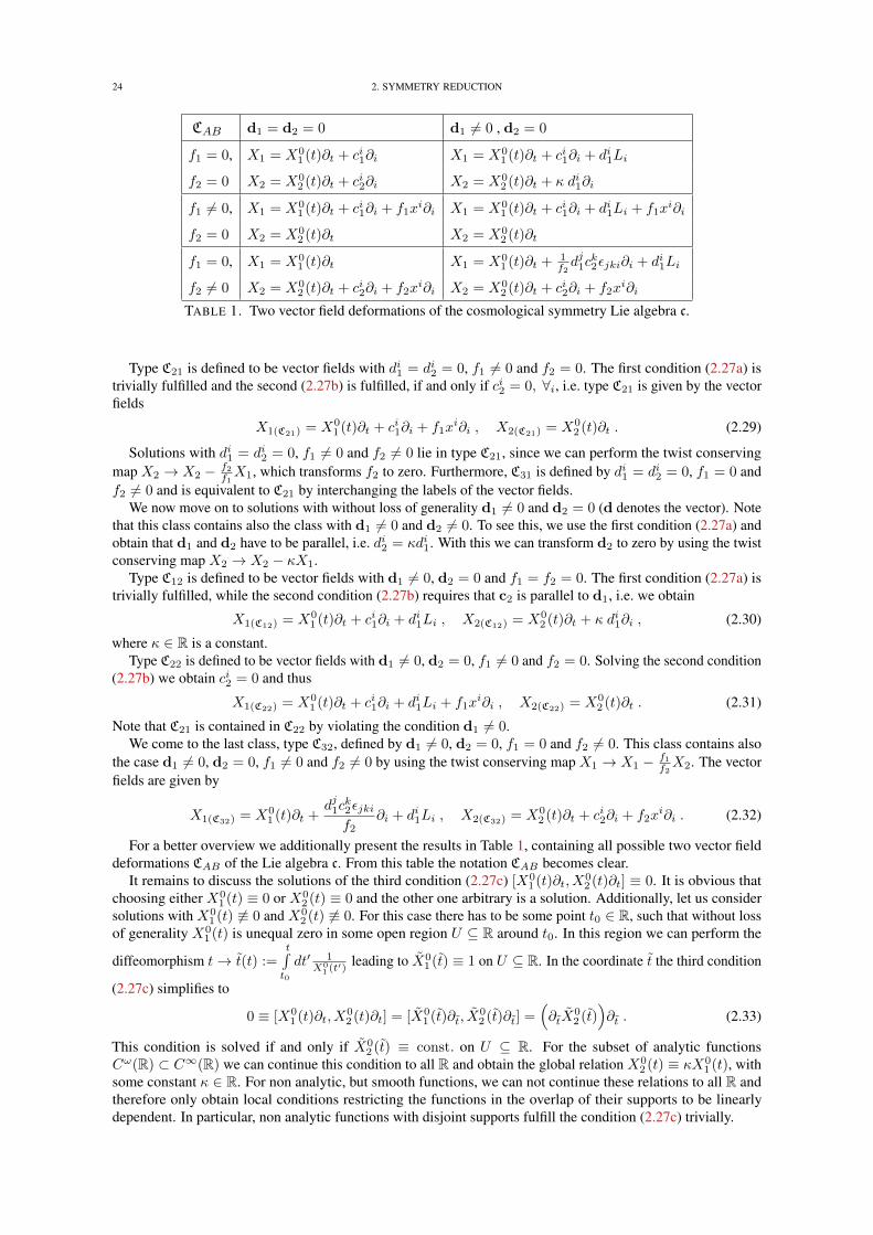
24 2. SYMMETRY REDUCTION

CAB d1 = d2 = 0 d1 6= 0 , d2 = 0

f1 = 0, X1 = X01 (t)∂t + ci1∂i X1 = X0

1 (t)∂t + ci1∂i + di1Li

f2 = 0 X2 = X02 (t)∂t + ci2∂i X2 = X0

2 (t)∂t + κ di1∂i

f1 6= 0, X1 = X01 (t)∂t + ci1∂i + f1x

i∂i X1 = X01 (t)∂t + ci1∂i + di1Li + f1x

i∂i

f2 = 0 X2 = X02 (t)∂t X2 = X0

2 (t)∂t

f1 = 0, X1 = X01 (t)∂t X1 = X0

1 (t)∂t + 1f2dj1c

k2εjki∂i + di1Li

f2 6= 0 X2 = X02 (t)∂t + ci2∂i + f2x

i∂i X2 = X02 (t)∂t + ci2∂i + f2x

i∂i

TABLE 1. Two vector field deformations of the cosmological symmetry Lie algebra c.

Type C21 is defined to be vector fields with di1 = di2 = 0, f1 6= 0 and f2 = 0. The first condition (2.27a) istrivially fulfilled and the second (2.27b) is fulfilled, if and only if ci2 = 0, ∀i, i.e. type C21 is given by the vectorfields

X1(C21) = X01 (t)∂t + ci1∂i + f1x

i∂i , X2(C21) = X02 (t)∂t . (2.29)

Solutions with di1 = di2 = 0, f1 6= 0 and f2 6= 0 lie in type C21, since we can perform the twist conservingmap X2 → X2 − f2

f1X1, which transforms f2 to zero. Furthermore, C31 is defined by di1 = di2 = 0, f1 = 0 and

f2 6= 0 and is equivalent to C21 by interchanging the labels of the vector fields.We now move on to solutions with without loss of generality d1 6= 0 and d2 = 0 (d denotes the vector). Note

that this class contains also the class with d1 6= 0 and d2 6= 0. To see this, we use the first condition (2.27a) andobtain that d1 and d2 have to be parallel, i.e. di2 = κdi1. With this we can transform d2 to zero by using the twistconserving map X2 → X2 − κX1.

Type C12 is defined to be vector fields with d1 6= 0, d2 = 0 and f1 = f2 = 0. The first condition (2.27a) istrivially fulfilled, while the second condition (2.27b) requires that c2 is parallel to d1, i.e. we obtain

X1(C12) = X01 (t)∂t + ci1∂i + di1Li , X2(C12) = X0

2 (t)∂t + κ di1∂i , (2.30)

where κ ∈ R is a constant.Type C22 is defined to be vector fields with d1 6= 0, d2 = 0, f1 6= 0 and f2 = 0. Solving the second condition

(2.27b) we obtain ci2 = 0 and thus

X1(C22) = X01 (t)∂t + ci1∂i + di1Li + f1x

i∂i , X2(C22) = X02 (t)∂t . (2.31)

Note that C21 is contained in C22 by violating the condition d1 6= 0.We come to the last class, type C32, defined by d1 6= 0, d2 = 0, f1 = 0 and f2 6= 0. This class contains also

the case d1 6= 0, d2 = 0, f1 6= 0 and f2 6= 0 by using the twist conserving map X1 → X1 − f1

f2X2. The vector

fields are given by

X1(C32) = X01 (t)∂t +

dj1ck2εjkif2

∂i + di1Li , X2(C32) = X02 (t)∂t + ci2∂i + f2x

i∂i . (2.32)

For a better overview we additionally present the results in Table 1, containing all possible two vector fielddeformations CAB of the Lie algebra c. From this table the notation CAB becomes clear.

It remains to discuss the solutions of the third condition (2.27c) [X01 (t)∂t, X

02 (t)∂t] ≡ 0. It is obvious that

choosing either X01 (t) ≡ 0 or X0

2 (t) ≡ 0 and the other one arbitrary is a solution. Additionally, let us considersolutions with X0

1 (t) 6≡ 0 and X02 (t) 6≡ 0. For this case there has to be some point t0 ∈ R, such that without loss

of generality X01 (t) is unequal zero in some open region U ⊆ R around t0. In this region we can perform the

diffeomorphism t→ t(t) :=t∫t0

dt′ 1X0

1 (t′)leading to X0

1 (t) ≡ 1 on U ⊆ R. In the coordinate t the third condition

(2.27c) simplifies to

0 ≡ [X01 (t)∂t, X

02 (t)∂t] = [X0

1 (t)∂t, X02 (t)∂t] =

(∂tX

02 (t)

)∂t . (2.33)

This condition is solved if and only if X02 (t) ≡ const. on U ⊆ R. For the subset of analytic functions

Cω(R) ⊂ C∞(R) we can continue this condition to all R and obtain the global relation X02 (t) ≡ κX0

1 (t), withsome constant κ ∈ R. For non analytic, but smooth functions, we can not continue these relations to all R andtherefore only obtain local conditions restricting the functions in the overlap of their supports to be linearlydependent. In particular, non analytic functions with disjoint supports fulfill the condition (2.27c) trivially.

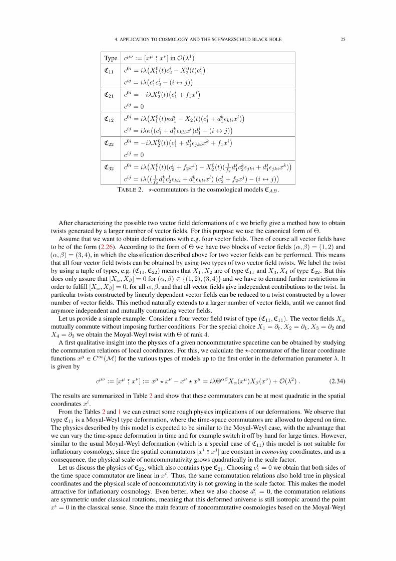
4. APPLICATION TO COSMOLOGY AND THE SCHWARZSCHILD BLACK HOLE 25

Type cµν := [xµ ?, xν ] in O(λ1)

C11 c0i = iλ(X0

1 (t)ci2 −X02 (t)ci1

)cij = iλ

(ci1c

j2 − (i↔ j)

)C21 c0i = −iλX0

2 (t)(ci1 + f1x

i)

cij = 0

C12 c0i = iλ(X0

1 (t)κdi1 −X2(t)(ci1 + dk1εklixl))

cij = iλκ((ci1 + dk1εklix

l)dj1 − (i↔ j))

C22 c0i = −iλX02 (t)

(ci1 + dj1εjkix

k + f1xi)

cij = 0

C32 c0i = iλ(X0

1 (t)(ci2 + f2xi)−X0

2 (t)( 1f2dj1c

k2εjki + dj1εjkix

k))

cij = iλ(( 1f2dk1c

l2εkli + dk1εklix

l) (cj2 + f2xj)− (i↔ j)

)TABLE 2. ?-commutators in the cosmological models CAB .

After characterizing the possible two vector field deformations of c we briefly give a method how to obtaintwists generated by a larger number of vector fields. For this purpose we use the canonical form of Θ.

Assume that we want to obtain deformations with e.g. four vector fields. Then of course all vector fields haveto be of the form (2.26). According to the form of Θ we have two blocks of vector fields (α, β) = (1, 2) and(α, β) = (3, 4), in which the classification described above for two vector fields can be performed. This meansthat all four vector field twists can be obtained by using two types of two vector field twists. We label the twistby using a tuple of types, e.g. (C11,C22) means that X1, X2 are of type C11 and X3, X4 of type C22. But thisdoes only assure that [Xα, Xβ ] = 0 for (α, β) ∈ (1, 2), (3, 4) and we have to demand further restrictions inorder to fulfill [Xα, Xβ ] = 0, for all α, β, and that all vector fields give independent contributions to the twist. Inparticular twists constructed by linearly dependent vector fields can be reduced to a twist constructed by a lowernumber of vector fields. This method naturally extends to a larger number of vector fields, until we cannot findanymore independent and mutually commuting vector fields.

Let us provide a simple example: Consider a four vector field twist of type (C11,C11). The vector fields Xα

mutually commute without imposing further conditions. For the special choice X1 = ∂t, X2 = ∂1, X3 = ∂2 andX4 = ∂3 we obtain the Moyal-Weyl twist with Θ of rank 4.

A first qualitative insight into the physics of a given noncommutative spacetime can be obtained by studyingthe commutation relations of local coordinates. For this, we calculate the ?-commutator of the linear coordinatefunctions xµ ∈ C∞(M) for the various types of models up to the first order in the deformation parameter λ. Itis given by

cµν := [xµ ?, xν ] := xµ ? xν − xν ? xµ = iλΘαβXα(xµ)Xβ(xν) +O(λ2) . (2.34)

The results are summarized in Table 2 and show that these commutators can be at most quadratic in the spatialcoordinates xi.

From the Tables 2 and 1 we can extract some rough physics implications of our deformations. We observe thattype C11 is a Moyal-Weyl type deformation, where the time-space commutators are allowed to depend on time.The physics described by this model is expected to be similar to the Moyal-Weyl case, with the advantage thatwe can vary the time-space deformation in time and for example switch it off by hand for large times. However,similar to the usual Moyal-Weyl deformation (which is a special case of C11) this model is not suitable forinflationary cosmology, since the spatial commutators [xi ?, xj ] are constant in comoving coordinates, and as aconsequence, the physical scale of noncommutativity grows quadratically in the scale factor.

Let us discuss the physics of C22, which also contains type C21. Choosing ci1 = 0 we obtain that both sides ofthe time-space commutator are linear in xi. Thus, the same commutation relations also hold true in physicalcoordinates and the physical scale of noncommutativity is not growing in the scale factor. This makes the modelattractive for inflationary cosmology. Even better, when we also choose di1 = 0, the commutation relationsare symmetric under classical rotations, meaning that this deformed universe is still isotropic around the pointxi = 0 in the classical sense. Since the main feature of noncommutative cosmologies based on the Moyal-Weyl

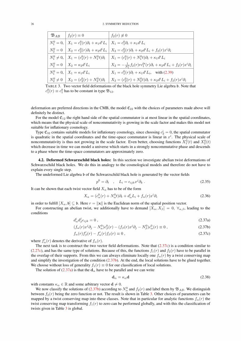
26 2. SYMMETRY REDUCTION

BAB f2(r) ≡ 0 f2(r) 6≡ 0

N01 = 0, X1 = c01(r)∂t + κ1d

iLi X1 = c01∂t + κ1diLi

N02 = 0 X2 = c02(r)∂t + κ2d

iLi X2 = c02(r)∂t + κ2diLi + f2(r)xi∂i

N01 6= 0, X1 = (c01(r) +N0

1 t)∂t X1 = (c01(r) +N01 t)∂t + κ1d

iLi

N02 = 0 X2 = κ2d

iLi X2 = − 1N0

1f2(r)rc0′1 (r)∂t + κ2d

iLi + f2(r)xi∂i

N01 = 0, X1 = κ1d

iLi X1 = c01(r)∂t + κ1diLi, with (2.39)

N02 6= 0 X2 = (c02(r) +N0

2 t)∂t X2 = (c02(r) +N02 t)∂t + κ2d

iLi + f2(r)xi∂i

TABLE 3. Two vector field deformations of the black hole symmetry Lie algebra b. Note thatc01(r) ≡ c01 has to be constant in type B12.

deformation are preferred directions in the CMB, the model C22 with the choices of parameters made above willdefinitely be distinct.

For the model C12 the right hand side of the spatial commutator is at most linear in the spatial coordinates,which means that the physical scale of noncommutativity is growing in the scale factor and makes this model notsuitable for inflationary cosmology.

Type C32 contains suitable models for inflationary cosmology, since choosing ci2 = 0, the spatial commutatoris quadratic in the spatial coordinates and the time-space commutator is linear in xi. The physical scale ofnoncommutativity is thus not growing in the scale factor. Even better, choosing functions X0

1 (t) and X02 (t)

which decrease in time we can model a universe which starts in a strongly noncommutative phase and descendsto a phase where the time-space commutators are approximately zero.

4.2. Deformed Schwarzschild black holes: In this section we investigate abelian twist deformations ofSchwarzschild black holes. We do this in analogy to the cosmological models and therefore do not have toexplain every single step.

The undeformed Lie algebra b of the Schwarzschild black hole is generated by the vector fields

p0 = ∂t , Li = εijkxj∂k . (2.35)

It can be shown that each twist vector field Xα has to be of the form

Xα = (c0α(r) +N0αt)∂t + diαLi + fα(r)xi∂i (2.36)

in order to fulfill [Xα, b] ⊆ b. Here r = ‖x‖ is the Euclidean norm of the spatial position vector.For constructing an abelian twist, we additionally have to demand [Xα, Xβ ] = 0, ∀α,β , leading to the

conditions

diαdjβεijk = 0 , (2.37a)

(fα(r)xj∂j −N0α)c0β(r)− (fβ(r)xj∂j −N0

β)c0α(r) ≡ 0 , (2.37b)

fα(r)f ′β(r)− f ′α(r)fβ(r) ≡ 0 , (2.37c)

where f ′α(r) denotes the derivative of fα(r).The next task is to construct the two vector field deformations. Note that (2.37c) is a condition similar to

(2.27c), and has the same type of solutions. Because of this, the functions f1(r) and f2(r) have to be parallel inthe overlap of their supports. From this we can always eliminate locally one fα(r) by a twist conserving mapand simplify the investigation of the condition (2.37b). At the end, the local solutions have to be glued together.We choose without loss of generality f1(r) ≡ 0 for our classification of local solutions.

The solution of (2.37a) is that the dα have to be parallel and we can write

dα = καd (2.38)

with constants κα ∈ R and some arbitrary vector d 6= 0.We now classify the solutions of (2.37b) according to N0

α and f2(r) and label them by BAB . We distinguishbetween f2(r) being the zero function or not. The result is shown in Table 3. Other choices of parameters can bemapped by a twist conserving map into these classes. Note that in particular for analytic functions fα(r) thetwist conserving map transforming f1(r) to zero can be performed globally, and with this the classification oftwists given in Table 3 is global.

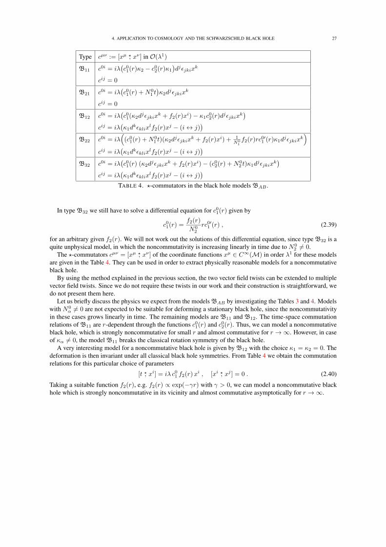
4. APPLICATION TO COSMOLOGY AND THE SCHWARZSCHILD BLACK HOLE 27

Type cµν := [xµ ?, xν ] in O(λ1)

B11 c0i = iλ(c01(r)κ2 − c02(r)κ1

)djεjkix

k

cij = 0

B21 c0i = iλ(c01(r) +N0

1 t)κ2d

jεjkixk

cij = 0

B12 c0i = iλ(c01(κ2d

jεjkixk + f2(r)xi)− κ1c

02(r)djεjkix

k)

cij = iλ(κ1d

kεklixlf2(r)xj − (i↔ j)

)B22 c0i = iλ

((c01(r) +N0

1 t)(κ2djεjkix

k + f2(r)xi) + 1N0

1f2(r)rc0′1 (r)κ1d

jεjkixk)

cij = iλ(κ1d

kεklixlf2(r)xj − (i↔ j)

)B32 c0i = iλ

(c01(r) (κ2d

jεjkixk + f2(r)xi)− (c02(r) +N0

2 t)κ1djεjkix

k)

cij = iλ(κ1d

kεklixlf2(r)xj − (i↔ j)

)TABLE 4. ?-commutators in the black hole models BAB .

In type B32 we still have to solve a differential equation for c01(r) given by

c01(r) =f2(r)

N02

rc0′1 (r) , (2.39)

for an arbitrary given f2(r). We will not work out the solutions of this differential equation, since type B32 is aquite unphysical model, in which the noncommutativity is increasing linearly in time due to N0

2 6= 0.The ?-commutators cµν = [xµ ?, xν ] of the coordinate functions xµ ∈ C∞(M) in order λ1 for these models

are given in the Table 4. They can be used in order to extract physically reasonable models for a noncommutativeblack hole.

By using the method explained in the previous section, the two vector field twists can be extended to multiplevector field twists. Since we do not require these twists in our work and their construction is straightforward, wedo not present them here.

Let us briefly discuss the physics we expect from the models BAB by investigating the Tables 3 and 4. Modelswith N0

α 6= 0 are not expected to be suitable for deforming a stationary black hole, since the noncommutativityin these cases grows linearly in time. The remaining models are B11 and B12. The time-space commutationrelations of B11 are r-dependent through the functions c01(r) and c02(r). Thus, we can model a noncommutativeblack hole, which is strongly noncommutative for small r and almost commutative for r →∞. However, in caseof κα 6= 0, the model B11 breaks the classical rotation symmetry of the black hole.

A very interesting model for a noncommutative black hole is given by B12 with the choice κ1 = κ2 = 0. Thedeformation is then invariant under all classical black hole symmetries. From Table 4 we obtain the commutationrelations for this particular choice of parameters

[t ?, xi] = iλ c01 f2(r)xi , [xi ?, xj ] = 0 . (2.40)

Taking a suitable function f2(r), e.g. f2(r) ∝ exp(−γr) with γ > 0, we can model a noncommutative blackhole which is strongly noncommutative in its vicinity and almost commutative asymptotically for r →∞.

CHAPTER 3

Exact solutions

In this chapter we discuss exact solutions of the noncommutative gravity theory introduced in Chapter 1.These results have been published in the research article [OS09a] and the proceedings article [Sch09]. We alsocomment briefly on the related work by Schupp and Solodukhin [SS07, SS09] and Aschieri and Castellani[AC10].

1. Noncommutative gravity in the nice basis

The noncommutative gravity theory presented in Chapter 1 is formulated in a highly abstract way in ordermake it suitable for mathematical studies. However, for practical applications it is convenient to express allformulae of noncommutative differential geometry and gravity in a suitable (local) basis of vector fields andone-forms. This allows for straightforward calculations using “indices” and helps us to understand explicitexamples in more detail. Rewriting noncommutative gravity in terms of a suitable basis of vector fields andone-forms is the subject of this section.

Using a generic local basis ea ∈ Ξ : a = 1, . . . , N of vector fields turns out to be not helpful for simplifyingthe formalism, since the R-matrices appearing in the formulae of Chapter 1 will complicate practical calculations.When we have discussed the example of the Moyal-Weyl deformation in Chapter 1, Section 5, we have observedthat the resulting formulae take a simple form and, in particular, no R-matrix appeared. The reason for this is thatthe basis ∂µ : µ = 1, . . . , N is invariant under the Moyal-Weyl twist, i.e. the twist is generated by a subspaceof vector fields which commute with all basis vector fields ∂µ. Assuming such an invariant basis to exist globallywould be too restrictive. However, as we will see in the next sections, for many of our models discussed in Chapter2, we can find for almost all points p ∈ M an open region U 3 p and a local basis ea ∈ Ξ : a = 1, . . . , N,such that the vector fields F ⊆ Ξ generating the twist commute with all ea. Even more, we obtain that we canchoose the ea to be mutually commuting, i.e. [ea, eb] = 0 for all a, b. A basis with these properties is called anice basis. After finishing our article [OS09a], it was shown in [AC10] that for a large class of abelian twistsa nice basis always exists for open regions around almost all points inM. The basic idea is to show that theopen submanifoldMreg ⊆M of regular point, i.e. points p ∈M where there is an open region U 3 p, such thatdim(span(Xα)) is constant on U , is dense inM. Under the assumption that for each p ∈Mreg there is an openregion U ⊆Mreg, such that ΘαβXα ⊗Xβ = ΘαβXα ⊗ Xβ , where the Xα are pointwise linearly independent,the abelian twist reduces locally to the Moyal-Weyl twist in an appropriate coordinate system on U . The existenceof a nice basis for the Moyal-Weyl deformation ensures the existence of a local nice basis for this class of abeliantwists around almost all points p ∈M. Deformed tensor fields and the ?-Levi-Civita connection are then treatedlocally onMreg and extended toM by demanding smoothness. Note that, in contrast to what was claimed in[AC10], the assumption stated above does not hold true for all abelian twists, meaning that not all abelian twistsreduce locally to the Moyal-Weyl twist. These deformations will be called exotic. A prime example of an exoticdeformation is given byM = R2 twisted with X1 = ∂x and X2 = y∂x, where x, y denote global coordinates.Using the normalization Θ12 = 1 we have ΘαβXα ⊗Xβ = ∂x ⊗ y∂x − y∂x ⊗ ∂x. The corresponding twist isnontrivial, since the tensor product is over C, even though the vector fields X1 and X2 are pointwise linearlydependent. As we have shown in the letter [SU10b], see also Chapter 8, Section 4, exotic deformations can leadto very interesting quantum field theories, which completely differ from the usual Moyal-Weyl deformation. Thisis expected, since the corresponding twists are not even locally of Moyal-Weyl type. Exotic deformations ofgravity are not yet completely understood and remain an interesting subject for future investigations. The mainproblem is the following: If we can not locally reduce the deformation to the Moyal-Weyl deformation, we cannot yet construct a ?-Levi-Civita connection, which is one of the main ingredients of noncommutative gravity.See, however, Chapter 16 for a possible way to circumvent this problem by quantizing directly commutativeLevi-Civita connections.

For the remaining part of this section let M be an N -dimensional smooth manifold and F ∈ UF ⊗ UFbe a Drinfel’d twist. We assume that we have around almost all points a local nice basis of vector fields

29

30 3. EXACT SOLUTIONS

ea ∈ Ξ : a = 1, . . . , N, i.e. [F, ea] = 0 and [ea, eb] = 0 for all a, b. This is in particular given for allnonexotic abelian Drinfel’d twist. All formulae which follow will be valid locally in this special basis.

As a consequence of the nice basis ea, the ?-dual basis θa ∈ Ω1 : a = 1, . . . , N is equal to theundeformed dual basis, since

δba = 〈ea, θb〉? = 〈fα(ea), fα(θb)〉 = 〈ea, θb〉 . (3.1)

The opposite ?-contraction satisfies

〈θb, ea〉? = 〈θb, ea〉 = 〈ea, θb〉 = δba , (3.2)

thus θb is dual to ea from both sides. Employing the Leibniz rule we find for all v ∈ F

0 = v(δba) = v(〈θb, ea〉) = 〈v(θb), ea〉 , (3.3)

which implies LF(θb) = 0 for all b, i.e. θb is an invariant basis of Ω1.Let τ ∈ T be an arbitrary (q, r)-tensor field. Due to the invariance of the bases ea and θb we have locally

the two equivalent expressions

τ = τa1...aqb1...br

θb1 ⊗A · · · ⊗A θbr ⊗A ea1⊗A · · · ⊗A eaq (3.4a)

= τa1...aqb1...br

? θb1 ⊗A? · · · ⊗A? θbr ⊗A? ea1 ⊗A? · · · ⊗A? eaq . (3.4b)

Note that the coefficient functions τa1...aqb1...br

in both expressions are identical and that the position where we putτa1...aqb1...br

does not matter, e.g. we can also write it on the right.Let O? be a ?-covariant derivative on Ξ. Using the local basis ea we define the Christoffel symbols

O?eaeb = Γ?cab ec = Γ?cab ? ec . (3.5)

Consider now a ?-covariant derivative O? on one-forms Ω1. In the local basis we can express it in terms ofChristoffel symbols

O?eaθb = Γ?bac θ

c = Γ?bac ? θc . (3.6)

Demanding compatibility between the ?-covariant derivative on Ξ and Ω1 we obtain

0 = ea(δcb) = ea(〈θc, eb〉?) = 〈O?eaθc, eb〉? + 〈θc,O?eaeb〉?

= 〈Γ?cad ? θd, eb〉? + 〈θc,Γ?dab ? ed〉? = Γ?cab + Γ?cab , (3.7)

i.e. we have Γ?cab = −Γ?cab. The ?-covariant derivative is extended to tensor fields via

O?eaτ =(ea(τ

a1...aqb1...br

)− τa1...aq

b...br? Γ?bab1 − · · ·+ τa1...a

b1...br? Γ

?aqaa

)θb1 ⊗A · · · ⊗A eaq . (3.8)

For mathematical details on this extension see Part III. We denote the coefficient functions of O?eaτ by(O?eaτ

)a1...aq

b1...br= ea(τ

a1...aqb1...br

)− τa1...aq

b...br? Γ?bab1 − · · ·+ τa1...a

b1...br? Γ

?aqaa . (3.9)

Note that τa1...aqb1...br

and Γ?cab in the expressions above are coefficient functions. This means that the action of eais the Lie derivative on functions and all ?-products are ?-products between functions and do not “act on theindices”.

The ?-torsion and ?-curvature of O? take a simple form in the nice basis ea. We obtain

Tor?(ea, eb) = (Γ?cab − Γ?cba)ec , (3.10)

and

Riem?(ea, eb, ec) =(ea(Γ?dbc )− eb(Γ?dac) + Γ?ebc ? Γ?dae − Γ?eac ? Γ?dbe

)ed . (3.11)

We denote the coefficient functions of these tensors by

T ?cab = Γ?cab − Γ?cba , (3.12a)

R? dabc = ea(Γ?dbc )− eb(Γ?dac) + Γ?ebc ? Γ?dae − Γ?eac ? Γ?dbe . (3.12b)

The coefficient functions of the ?-Ricci tensor are given by R?ab = R? ccab, where the sum over c is understood.

Let g = θa ⊗A θb gab = θa ⊗A? θb ? gab be a metric field. The coefficient functions are real gab = g∗ab(provided the basis is real), symmetric gab = gba and invertible as a matrix. The ?-inverse metric fieldg−1 = ea ⊗A eb gab = ea ⊗A? eb ? gab is given by the ?-inverse matrix

gab ? gbc = gcb ? gba = δca . (3.13)

2. COSMOLOGICAL SOLUTIONS 31

The ?-covariant derivative acts on the metric field as(O?eag

)bc

= ea(gbc)− gbc ? Γ?bab − gbc ? Γ?cac . (3.14)

We can now prove analogously to the undeformed case that there is a unique ?-Levi-Civita connection, i.e. a?-covariant derivative which is metric compatible and ?-torsion free. The steps in this proof are the same as inthe corresponding undeformed version of the theorem. First, we assume that there is a ?-Levi-Civita connection.As a consequence, we have

0 =(O?eag

)bc

+(O?ebg

)ac−(O?ecg

)ab

= ea(gbc) + eb(gac)− ec(gab)− gdc ? Γ?dab − gbd ? Γ?dac

− gdc ? Γ?dba − gad ? Γ?dbc + gdb ? Γ?dca + gad ? Γ?dcbT?cab=0

= ea(gbc) + eb(gac)− ec(gab)− 2 gcd ? Γ?dab . (3.15)

This yields an expression for Γ?cab in terms of the metric

Γ?cab =1

2gcd ?

(ea(gbd) + eb(gad)− ed(gab)

). (3.16)

Thus, the ?-Levi-Civita connection is unique. It also exists, since O? can be constructed from the Christoffelsymbols (3.16).

The ?-curvature scalar is given by

R? = gab ? R?ab (3.17)

and we obtain the ?-Einstein tensor

G?ab = R?ab −1

2gab ?R

? . (3.18)

For the ?-Levi-Civita connection (3.16), the ?-Einstein tensor only depends on the metric gab. The equation ofmotion for vacuum noncommutative Einstein gravity are thus given by

G?ab = 0 . (3.19)

We can couple the metric to a suitable deformed stress-energy tensor T ? = θa ⊗A θb T ?ab = θa ⊗A? θb ? T ?ab viathe equation

G?ab = 8πGN T?ab . (3.20)

The goal of the next two sections is to discuss explicit solutions of these equations.

2. Cosmological solutions

We study examples of exact noncommutative gravity solutions. For this we make use of the cosmologicalmodels investigated in Chapter 2, Section 4. These models allow for a consistent deformed symmetry reductionand thus are expected to be appropriate for noncommutative cosmology. From the discussion in Chapter 2,Section 4, we have obtained that for inflationary cosmology only the model C22 with ci1 = 0 and C32 with ci2 = 0are suitable, since for all other models the physical scale of noncommutativity grows in the scale factor1. Dueto inflation this would lead to a highly noncommutative late universe, which we consider as unphysical. Wesimplify our discussion and assume the functions X0

1 (t) and X02 (t) in model C22 and C32 to be analytic. The

vector fields Xα generating these twists are then given by

C22 : X1 = di1Li + f1xi∂i , X2 = X(t)∂t , (3.21a)

C32 : X1 = κ1X(t)∂t + di1Li , X2 = κ2X(t)∂t + f2xi∂i . (3.21b)

Here Li := εijkxj∂k are the generators of rotations.

We can understand our models better by choosing without loss of generality d1 = (0, 0, d) and transformingfrom Cartesian coordinates xi to spherical coordinates (r, ζ, φ). The vector fields then read

C22 : X1 = d∂φ + f1r∂r , X2 = X(t)∂t , (3.22a)

C32 : X1 = κ1X(t)∂t + d∂φ , X2 = κ2X(t)∂t + f2r∂r . (3.22b)

1 Note that for C22 we can also obtain a physically acceptable model for ci1 6= 0 by demanding a rapidly decreasing function X02 (t),

such that |a(t)X02 (t)| does not grow in time, where a(t) is the scale factor. For late times this model can be approximated by the same

model with di1 = f1 = 0 and is equivalent to a time-dependent Moyal-Weyl deformation. Since we are interested in non-Moyal-Weyldeformations, this model is not of too much interest for us and we do not discuss it further in the following.

32 3. EXACT SOLUTIONS

The nontrivial ?-commutation relations between appropriate functions in spherical coordinates are:

C22 :

[t ?, exp iφ] = 2 exp iφ sinh

(λd2X(t)∂t

)t

[t ?, r] = −2ir sin(λf2

2X(t)∂t

)t

(3.23a)

C32 :

[t ?, exp iφ] = 2 exp iφ sinh

(λdκ2

2X(t)∂t

)t

[t ?, r] = 2ir sin(λf2κ1

2X(t)∂t

)t

exp iφ ? r = e−λdf2 r ? exp iφ

(3.23b)

In particular, our models include time-angle, time-radius and angle-radius noncommutativity. Note that the?-commutators simplify dramatically for the choice X(t) ≡ 1. This will be further explained below, when wediscuss specific parameter choices in these models.

For our cosmological models we can make the following choice for a nice local basis of vector fields

e1 = X(t)∂t , e2 = r∂r , e3 = ∂ζ , e4 = ∂φ , if X(t) 6≡ 0 , (3.24a)

e1 = ∂t , e2 = r∂r , e3 = ∂ζ , e4 = ∂φ , if X(t) ≡ 0 . (3.24b)

The required conditions [ea, eb] = 0 and [Xα, eb] = 0 hold true for all a, b, α. Note that (3.24a) is only a localbasis in open regions around times t, where X(t) 6= 0. Since X(t) is assumed to be analytic, the points aroundwhich we do not have a nice basis are a null set inM. Knowing a smooth tensor field on this dense set, we canuse smoothness in order to extend it to all ofM.

Let us move on to exact cosmological solutions of the noncommutative Einstein equations. For this we canuse Proposition 2.2 in order to find the right ansatz for the symmetry reduced metric field g. This propositiontells us that a tensor field is invariant under the deformed action of the deformed symmetries, if and only if it isinvariant under the undeformed action of the undeformed symmetries. We make the ansatz g = dxµ ⊗A dxνgµνin the commutative coordinate basis with

gµν = diag(−1, a(t)2, a(t)2, a(t)2

)µν, (3.25)

and calculate the required coefficient functions gab in the nice basis by solving

θa ⊗A θbgab = dxµ ⊗A dxνgµν , (3.26)

using the explicit expressions for the nice basis vector fields (3.24).It can be checked explicitly that for the choice f1 = 0 in model C22 (3.22a) and the choice κ1 = 0 in model

C32 (3.22b) the ?-Levi-Civita connection (3.16), the ?-Riemann tensor (3.12b) and finally the ?-Einstein tensor(3.18) receive no contributions in the deformation parameter λ, thus reducing to the undeformed counterparts.The reason is that, for the restrictions mentioned above, one twist vector field Xα ∈ c is a Killing vector fieldand therefore deformed operations among invariant tensor fields reduce to the undeformed ones, since Xα ∈ cannihilates the tensors due to invariance.

Since the noncommutative stress-energy tensor of symmetry reduced matter fields reduces to the undeformedone due to the same reason, these noncommutative models are exactly solvable, if the undeformed model isexactly solvable. Note that the reduction of the deformed symmetry reduced tensor fields to the undeformedones does not mean that our models are trivial. In particular, we will obtain in general a deformed dynamics forfluctuations on the symmetry reduced backgrounds (see Part II), as well as a nontrivial coordinate algebra (3.23).

Let us discuss physical implications of the nontrivial coordinate algebras of our models. Consider the modelC22 (3.22a) with f1 = 0 and for simplicity X(t) ≡ 1. The coordinate algebra (3.23a) reduces to the algebra of aquantum mechanical particle on the circle, i. e.

[t, E] = λE , (3.27)

where we have introduced the abstract operators t and E := exp iφ and set d = 1. This algebra previouslyappeared e.g. in the context of noncommutative field theory [CDPT01, BGMTS04] and the noncommutativeBTZ black hole [DGS07]. It is well-known that the operator t can be represented as a differential operatoracting on the Hilbert space L2(S1) of square integrable functions on the circle and the spectrum can be shownto be given by σ(t) = λ(Z + δ), where δ ∈ [0, 1) labels unitary inequivalent representations. The spectrumshould be interpreted as possible time eigenvalues, i.e. our model has a discrete time. This feature can be used torealize singularity avoidance in cosmology. Consider for example an inflationary background with a(t) = tp,where p > 1 is a parameter. This so-called power-law inflation can be realized by coupling a scalar field

3. BLACK HOLE SOLUTIONS 33

with exponential potential to the geometry even in our noncommutative model, since the symmetry reducednoncommutative gravity theory reduces to the undeformed one as explained above. Note that the scale factorgoes to zero at the time t = 0 and leads to a singularity in the curvature scalar. But as we have discussed above,the possible time eigenvalues are λ(Z + δ), which does not include the time t = 0 for δ 6= 0.

For the more complicated solvable model C32 (3.22b) with κ1 = 0 we obtain time-angle and angle-radiusnoncommutativity. We set without loss of generality the parameters d = f2 = 1. Firstly, we choose X(t) ≡ 0leading to a pure angle-radius noncommutativity. The algebra (3.23b) becomes in this case

Er = e−λ rE . (3.28)

This algebra can be represented on the Hilbert space L2(S1) as

E = exp iφ , r = L exp(−iλ∂φ

), (3.29)

leading to the spectrum σ(r) = L exp(λ(Z + δ)

), where δ ∈ [0, 1) is again a parameter labeling unitary

inequivalent representations and L is some length scale. The radius becomes discrete. Note that this modeldescribes a kind of “condensating geometry” around the origin r = 0, since the shells of constant r accumulateat this point.

Secondly, we choose X(t) ≡ 1 in (3.23b). We obtain the abstract algebra

[t, E] = λE , Er = e−λ rE . (3.30)

We find the representation on L2(S1)

E = exp iφ , t = τ 1− iλ∂φ , r = L exp(−iλ∂φ

). (3.31)

Note that we had to introduce a real parameter τ ∈ R and the identity operator 1 in order to cover the wholespacetime.

The last cosmological model we want to briefly discuss is the isotropic model C22 with d = 0 (3.22a). It turnsout that both Xα are not Killing vector fields and the symmetry reduced noncommutative gravity theory doesnot automatically reduce to the undeformed one. Thus, we expect corrections in λ to the ?-Einstein equations(3.18) and its solutions. However, we have found a special exact solution of this model which is physically veryinteresting.

Consider the (undeformed) de Sitter space given by a(t) = expHt, where H is the Hubble parameter. It turnsout that all ?-products entering the deformed geometrical quantities reduce to the undeformed ones, if X(t) ≡ 1.Thus, the undeformed de Sitter space solves exactly the ?-Einstein equations in presence of a cosmologicalconstant for this particular choice of twist. Note that in contrast to the solutions above, we have required theexplicit form of the scale factor a(t).

3. Black hole solutions

We now turn to examples of noncommutative black hole solutions, making use of the models investigated inChapter 2, Section 4. From the discussion in this section we found that the only physically viable noncommutativeblack hole models are B11 and B12, since all other models have a noncommutativity growing linearly in time.As a reminder, the twist generating vector fields Xα for these models are given by

B11 : X1 = c01(r)∂t + κ1diLi , X2 = c02(r)∂t , (3.32a)

B12 : X1 = c01∂t + κ1diLi , X2 = c02(r)∂t + κ2d

iLi + f2(r)xi∂i , (3.32b)

where c01 in B12 has to be constant and r := ‖x‖ is the radial coordinate. We have set without loss of generalityκ2 = 0 in B11. Let us again choose d = (0, 0, d) and transform from Cartesian coordinates xi to sphericalcoordinates (r, ζ, φ). The twist generating vector fields read in this basis

B11 : X1 = c01(r)∂t + κ1∂φ , X2 = c02(r)∂t , (3.33a)

B12 : X1 = c01∂t + κ1∂φ , X2 = c02(r)∂t + κ2∂φ + f(r)∂r . (3.33b)

34 3. EXACT SOLUTIONS

Note that we have defined f(r) := f2(r)r and absorbed the parameter d into κα in order to simplify theexpressions. The nontrivial ?-commutation relations between appropriate functions in spherical coordinates are:

B11 :

[t ?, exp iφ] = λ exp iφ κ1c02(r) (3.34a)

B12 :

[t ?, exp iφ] = exp iφ

(2 sinh

(λκ1

2

(c02(r)∂t + f(r)∂r

))t− λκ2c

01

)[t ?, r] = iλc01f(r)

[exp iφ ?, r] = −2 exp iφ sinh(λκ1

2f(r)∂r

)r

(3.34b)

In particular, our models include time-angle, time-radius and angle-radius noncommutativity. Note that the?-commutators simplify dramatically for the choice f(r) = r and c02(r) ≡ const.. This will be further explainedbelow, when we discuss specific choices for the parameters.

We now study for which parameter choices the deformation is nonexotic. This is required to set up thenoncommutative Einstein equations. We assume that c01(r), c02(r) and f(r) are analytic functions to simplify theinvestigations. Model B11 is nonexotic for κ1 6= 0. A nice basis is given by

e1 = X2 , e2 = ∂r + tc0′2 (r)

c02(r)∂t +

φ

κ1

(c0′1 (r)− c01(r)c0′2 (r)

c02(r)

)∂t, e3 = ∂ζ , e4 = X1 , (3.35a)

where c0′1 (r) and c0′2 (r) denotes the derivative of c01(r) and c02(r), respectively. This basis is only defined in openregions around radii r satisfying c02(r) 6= 0 and on φ ∈ (0, 2π) (due to the term linear in φ). Since c02(r) 6≡ 0 isassumed to be nonvanishing in order to have a nontrivial deformation and analytic, this is a dense set inM.

We now come to B12 with f(r) 6≡ 0 (otherwise B12 becomes part of B11). This model is nonexotic and wefind the nice basis

e1 = ∂t , e2 = f(r)∂r + c02(r)∂t , e3 = ∂ζ , e4 = ∂φ , (3.35b)

which is defined in open regions around radii r with f(r) 6= 0. Since f(r) is assumed to be analytic this set isdense inM.

We use again Proposition 2.2 and make the ansatz

gµν = diag(−Q(r), S(r), r2, (r sin ζ)2

)µν

(3.36)

for the metric field g = dxµ ⊗A dxνgµν in the commutative spherical coordinate basis. The metric in the nicebasis can be calculated using (3.35a) or (3.35b), respectively. Concerning the solution of the ?-Einstein equationswe are in a comfortable position, since X1 ∈ b in B12 is a Killing vector field, which means that the symmetryreduced noncommutative gravity theory reduces to the undeformed one. Choosing in B11 either c01(r) ≡ const.or c02(r) ≡ const., we obtain X1 ∈ b or X2 ∈ b. Note that in this case B11 becomes part of type B12 by settingf(r) ≡ 0. This leads in the exterior of our noncommutative black hole to the metric (3.36) with

Q(r) = S(r)−1 = 1− rsr, (3.37)

where rs is the Schwarzschild radius. As in the case of the cosmological models, the reduction of the symmetryreduced tensor fields to the undeformed counterparts does not mean that our models are trivial. Field fluctuations,as well as the coordinate algebras, will in general receive distinct noncommutative effects.

Taking a look at the coordinate algebra of the black hole B12 (3.34b), we observe that it includes in particularthe algebra of a quantum mechanical particle on the circle for the time and angle coordinate, if we choosec02(r) ≡ 0 and f(r) ≡ 0. This leads to discrete times. Another simple choice is c01 = κ2 = 0, c02(r) ≡ 0, κ1 = 1and f(r) = r. The radius spectrum in this case is σ(r) = L exp

(λ(Z + δ)

), describing a fine grained geometry

around the black hole. The phenomenological problem with this model is that the spacings between the radiuseigenvalues grow exponentially in r. This can be fixed by considering a modified twist like e. g. c01 = κ2 = 0,c02(r) ≡ 0, κ1 = 1 and f(r) = tanh r

L , where L is some length scale. The essential modification is to choosea bounded f(r). Consider the coordinate change r → η = log sinh( rL ). Note that r and not η is the physicalradial coordinate of a Schwarzschild observer, η is just introduced in order to simplify the calculation. In termsof η the algebra (3.34b) reduces to

[E, η] = −λLE , (3.38)

leading to the spectrum σ(η) = λL

(Z + δ

). The spectrum of the physical radius r is then given by σ(r) =

L arcsinh exp(λL (Z + δ)

). This spectrum approaches constant spacings between the eigenvalues for large r.

4. GENERAL STATEMENT ON NONCOMMUTATIVE GRAVITY SOLUTIONS 35

As a last model we consider B12 with κ1 = κ2 = 0, c02(r) ≡ 0 and the normalization c01 = 1. This model isinvariant under all classical black hole symmetries. The nontrivial commutation relation is given by

[t, r] = i λ f(r) . (3.39)

For the special case f(r) = r we obtain the κ-commutation relations [t, r] = i λ r. The κ-commutation relationscan be represented on L2(R) by the operators

t = −iλ ∂

∂s, r = Le−s . (3.40)

This representation is unique up to unitary equivalence [DP10]. The spectrum of the time and radius operatoris σ(t) = R and σ(r) = (0,∞), respectively. Thus, there is no discretization of time or radius, however, thisspacetime is noncommutative which leads to distinct effects in the propagation of fields (see Part II).

We omit a discussion of further possible models, since our main goal was to present the very explicit andsimple examples shown above. We conclude this section with one remark. Our class of black hole models (3.33b)has a nonvanishing overlap with the noncommutative black hole models found before by Schupp and Solodukhin[SS07, SS09]. They also observed that the symmetry reduced dynamics reduces to the undeformed one, providedthe deformation is constructed by sufficiently many Killing vector fields. In addition, they have constructedmodels based on a nonabelian and projective twist, that is not part of the class of abelian twists we have used forour investigations. Their black holes exhibit discrete radius eigenvalues as well.

4. General statement on noncommutative gravity solutions

After studying explicit examples of exact solutions of the noncommutative Einstein equations, we gathereda sufficient understanding in order to make more general statements on solutions [SS07, SS09, OS09a, AC10].Let g be a classical metric field and Φii∈I be a collection of classical matter fields which are invariant undersome symmetry Lie algebra g ⊆ Ξ and solve classical Einstein equations and geometric differential equationsfor Φii∈I . Consider a deformation by a nonexotic abelian Drinfel’d twist (2.7) with linearly independentXα. If now either the vector field Xα or Xα = ΘβαXβ is a Killing vector field for all α, then the classicalsolutions g and Φi also solve the noncommutative Einstein equations and the corresponding deformed geometricdifferential equations for Φi. Let us explain why: Because everything is assumed to be smooth, it is sufficient tocheck if the noncommutative equations of motion are solved in open regions around every regular point. In theseregions we can choose a nice basis ea satisfying [ea, eb] = 0 and [Xα, ea] = 0, for all a, b, α, and its dualθa satisfying LXα(θb) = 0, for all b, α. Writing a generic g-invariant tensor field in this basis, the coefficientfunctions will be annihilated by all Xα and Xα which are Killing vector fields, since the basis is invariantunder these transformations. From the formulae of Section 1 in this chapter we find that all deformed geometricquantities are calculated in the nice basis by using ?-products between coefficient functions. The ?-productsbetween g-invariant tensor coefficient functions drop out, since either Xα or Xα is a Killing vector field for allα. The deformed equations of motion then agree with the undeformed ones and thus are solved exactly. Let usmention again that the equations of motion for fluctuations around the g-invariant sector obtain noncommutativecorrections, see Part II.

CHAPTER 4

Open problems

In this chapter we comment on open problems in the noncommutative gravity theory [ADMW06], which wehave found during our investigations.

Exotic deformations and global approach: As discussed in detail above, the existence of a local nicebasis of vector fields is guaranteed only in case of nonexotic abelian twists, i.e. Drinfel’d twists which reduceto the Moyal-Weyl twist in open regions around almost all points inM. However, for the present formulationof noncommutative gravity, this nice basis of vector fields is required, since otherwise we can not yet provethe existence and uniqueness of a ?-Levi-Civita connection, one of the main ingredients of noncommutativegravity. As discussed in Chapter 8, Section 4, there are very interesting exotic deformations of scalar quantumfield theories, which might also be relevant for noncommutative gravity. Therefore, it is important to understandnoncommutative gravity beyond the nice basis.

Another motivation for a global and basis free understanding of noncommutative gravity comes from conver-gent deformations. As compared to formal deformations, the localization in open regions around points becomesimpossible in the convergent setting, since the twist acts as a nonlocal operator and in general does not preservethese patches. This means that we can not use a local nice basis in the convergent case, but we have to workin a global approach. A first step towards convergent deformations is thus to understand formal deformationson a global level, without referring to any local bases. This is a motivation for our global investigations onnoncommutative gravity in Part III. As a first successful application of this formalism we are going to study inChapter 16 solutions of the noncommutative Einstein equations in a global approach.

Inverse metric field: Since this problem also occurs for the Moyal-Weyl deformation of RN , we restrictourselves to this case in order to make our argument simple. Consider a metric field g = dxµ ⊗A? dxν ? gµν =dxµ⊗A dxνgµν , where we have used that dxµ is invariant under the twist. By definition, the metric is symmetricgµν = gνµ and real g∗µν = gµν . However, the inverse metric field g−1 = gµν∂µ ⊗A ∂ν defined by

gµν ? gνρ = gρν ? gνµ = δρµ (4.1)

is in general neither symmetric nor real, but only hermitian gµν∗ = gνµ. This leads to an asymmetry between themetric field and its inverse, and the question arises which one we should demand to be symmetric and real, thuspaying the price that the other one is only hermitian. Another option is to use hermitian metrics for formulatingnoncommutative gravity, see e.g. [CFF93, Cha01], which however leads to new degrees of freedom compared toEinstein’s gravity.

A further issue is that the ?-Levi-Civita connection is in general not compatible with the inverse metric. Tosee this, let us again focus on the Moyal-Weyl deformation of RN . The Christoffel symbols of the ?-Levi-Civitaconnection are uniquely defined by symmetry Γ?ρµν = Γ?ρνµ and metric compatibility

0 = ∂µgνρ − gτρ ? Γ?τµν − gντ ? Γ?τµρ , (4.2)

yielding the expression

Γ?ρµν =1

2gρσ ?

(∂µgνσ + ∂νgµσ − ∂σgµν

). (4.3)

As a consequence of (4.1) the inverse metric satisfies

0 = ∂µgνρ + Γ?νµσ ? g

σρ + gνε ? gτσ ? Γ?τµε ? gσρ . (4.4)

For noncentral Christoffel symbols this leads to a violation of the compatibility condition for the inverse metric,i.e.

0 6= ∂µgνρ + gτρ ? Γ?νµτ + gντ ? Γ?ρµτ . (4.5)

37

38 4. OPEN PROBLEMS

To be explicit, we consider a conformally flat metric field gµν = Φ ηµν , where Φ is a positive definite functionand ηµν is the Minkowski metric. The Christoffel symbols read

Γ?ρµν =1

2Φ−1? ?

(∂µΦδρν + ∂νΦδρµ − ∂ρΦηµν

), (4.6)

where the index of ∂ρ is raised with the Minkowski metric and Φ−1? is the ?-inverse function of Φ. We obtain

∂µgνρ + gτρ ? Γ?νµτ + gντ ? Γ?ρµτ =

(∂µΦ−1? + Φ−2? ? ∂µΦ

)ηνρ

=(−Φ−1? ? ∂µΦ ? Φ−1? + Φ−2? ? ∂µΦ

)ηνρ 6= 0 . (4.7)

Covariant derivatives and their extension: One problem which we could solve in this thesis is theextension of covariant derivatives to tensor fields, see Part III. To understand why this improvement wasnecessary, we show explicitly where the original definition of [ADMW06] breaks down. As a reminder, a?-covariant derivative is defined to be a C-linear map O?u : Ξ→ Ξ satisfying

O?v+wz = O?vz + O?wz , (4.8a)

O?h?vz = h ? O?vz , (4.8b)

O?v(h ? z) = L?v(h) ? z + Rα(h) ? O?Rα(v)z . (4.8c)

The extension of the ?-covariant derivative to bivector fields Ξ⊗A? Ξ was given in [ADMW06] by

O?v(w ⊗A? z) =(O?vw

)⊗A? z + Rα(w)⊗A? O?Rα(v)z . (4.9)

Let us study this equation in more detail for the Moyal-Weyl deformation of RN . By definition of the ?-tensorproduct and invariance of the basis ∂µ we have (h ? ∂ν) ⊗A? ∂ρ = ∂ν ⊗A? (h ? ∂ρ), for all functions h. The?-covariant derivative should respect this middle linearity property in order to be well-defined. However, we findfor (4.9) by an explicit calculation

O?∂µ((h ? ∂ν)⊗A? ∂ρ) = O?∂µ(h ? ∂ν)⊗A? ∂ρ + h ? ∂ν ⊗A? O?∂ν∂ρ= ∂µh ? ∂ν ⊗A? ∂ρ + h ?

(O?∂µ∂ν ⊗A? ∂ρ + ∂ν ⊗A? O?∂µ∂ρ

)(4.10a)

and

O?∂µ(∂ν ⊗A? (h ? ∂ρ)) = O?∂µ∂ν ⊗A? h ? ∂ρ + ∂ν ⊗A? O?∂µ(h ? ∂ρ)

= O?∂µ∂ν ⊗A? h ? ∂ρ + ∂ν ⊗A? ∂µh ? ∂ρ + ∂ν ⊗A? h ? O?∂µ∂ρ= ∂µh ? ∂ν ⊗A? ∂ρ + O?∂µ∂ν ⊗A? h ? ∂ρ + h ? ∂ν ⊗A? O?∂µ∂ρ . (4.10b)

Note that the second term of (4.10a) is different to (4.10b) in case the Christoffel symbols are noncentral, whichis the generic case. This problem has been resolved and we show in Chapter 14 that there is a consistent definitionof a ?-covariant derivative on tensor fields.

Einstein tensor: As already discussed above, there are issues concerning the reality of the inverse metricfield. Similarly, the ?-curvature and ?-Einstein tensor turn out to be not real. To show this explicitly let us consideragain the Moyal-Weyl deformation of RN and a conformally flat metric field gµν = Φ ηµν . The Christoffelsymbols read

Γ?ρµν =1

2Φ−1? ?

(∂µΦδρν + ∂νΦδρµ − ∂ρΦηµν

)=: uµδ

ρν + uνδ

ρµ − uρηµν , (4.11)

where we have defined uµ = Φ−1? ? ∂µΦ/2. The ?-Ricci tensor reads

R?µν = ∂νuµ − (N − 1)∂µuν − ∂ρuρ ηµν + (N − 2)(uµ ? uν − uρ ? uρ ηµν

)(4.12)

and for the ?-curvature scalar we find

R? = Φ−1? ?(

2(1−N) ∂µuµ − (N − 2)(N − 1)uµ ? u

µ). (4.13)

Complex conjugation yields

u∗µ = Φ ? uµ ? Φ−1? , (∂µuν)∗ = Φ ? ∂νuµ ? Φ−1? . (4.14)

Using this we find for the ?-Ricci tensor and the ?-curvature scalar(R?µν

)∗= Φ ? R?νµ ? Φ−1? ,

(R?)∗

= Φ2? ?R? ? Φ−2? . (4.15)

The conjugation of the ?-Einstein tensor is(G?µν

)∗= Φ ? G?νµ ? Φ−1? . (4.16)

4. OPEN PROBLEMS 39

Reality (or hermiticity) of the ?-Einstein tensor is an essential aspect of noncommutative gravity. Demandingthe metric field to be real and symmetric (or hermitian), it is important that the dynamics preserves this property.From (4.16) one could expect that there is a modified hermiticity property, namely hermiticity up to ?-conjugationby Φ. Whether this is an artefact of using a conformally flat metric field is not yet clear.

Discussion: Even though the present formulation of noncommutative gravity is plagued by some unsolvedissues, the discussion of our exact solutions in Chapter 3 is not affected by these problems. The reason is that wehave considered symmetric spacetimes and we have chosen the deformation such that the symmetry reduced sectorof noncommutative gravity is undeformed. This would also hold true for modified noncommutative Einsteinequations, provided they are constructed according to the principle of deformed general covariance, i.e. by a twist.However, for investigating gravitational fluctuations around these highly symmetric noncommutative gravitybackgrounds, a more complete understanding of noncommutative gravity is required. Since noncommutativegravitons are not only important to study the stability of noncommutative gravity solutions, but they are also ofinterest in cosmological applications, we have resolve the issues which are present in the current formulation.This has been the main motivation for Part III of this thesis.

Part II

Quantum Field Theory on NoncommutativeCurved Spacetimes

CHAPTER 5

Basics

We review the algebraic approach to quantum field theory on commutative curved spacetimes following mostly[BGP07]. The focus is on a non-selfinteracting real scalar quantum field, which is coupled to a given classicalgravitational background.

1. Motivation

Quantum field theory on commutative curved spacetimes is by now a well established and far developed theory,see e.g. [Wal94, BGP07, BF09]. Early investigations on these theories have shown that the quantum field theoryon a generic curved spacetime differs drastically from the usual quantum field theory on the Minkowski spacetime,as presented in every introductory textbook. The main difference is that while on Minkowski spacetime we havea unique vacuum state for the quantum field theory, this uniqueness fails to be present in general. This is becausethe Minkowski spacetime has a very large isometry group, the Poincare group, which poses strong restrictions onpossible vacua, while a generic spacetime has no isometries. We therefore do not have sufficiently many criteriaat hand to choose from the huge space of all states a distinct one. Since Stone-von Neumann’s theorem does nothold true for infinitely may degrees of freedom, as in quantum field theory, different choices of vacuum states canlead to physically distinct predictions, because the corresponding Hilbert space representations are not unitaryequivalent. In other words, the choice of vacuum is an input we have to make which influences the physics resultswe extract from the quantum field theory. Another new feature one has to deal with when going from Minkowskito a generic spacetime is that the concept of particles becomes observer dependent. On Minkowski spacetime wehave preferred observers, living in an inertial frame, and all of them agree when measuring the particle numberof a state. However, for noninertial observers, such as the Unruh observer which moves in some direction with aconstant acceleration a, there is not anymore an agreement in the measured particle number, in particular, theUnruh observer “sees” the Minkowski vacuum state as a thermal state with temperature T = a/(2π) in naturalunits. Since on a generic spacetime there are no preferred observers, there is also no preferred notion of particles.Hence, on curved spacetimes quantum field theory is indeed a theory of fields and not of particles.

Due to the nonuniqueness of the vacuum state we have to treat all possible states on the same footing andit is therefore not convenient to start with a specific Hilbert space representation from the beginning. This isthe reason why quantum field theories on curved spacetimes are typically treated in the algebraic framework.The basic idea of this approach is to split the problem of constructing the quantum field theory into two steps:Firstly, one constructs an abstract algebra of observables for the quantum field theory, which should include theobservables we can in principle measure. Some properties of these observables can already be studied withoutreferring to a representation. In the second step, one considers algebraic states on this algebra, which associate toevery observable operator its expectation value. The connection to the usual framework of quantum field theoryusing Hilbert spaces is then made by constructing from the algebra and state the GNS-representation.

2. Some basics of Lorentzian geometry

We introduce some basic notions of Lorentzian geometry which will appear frequently in this part. We followthe presentation of [BGP07], since it is suitable for our purposes. More details and a thorough introduction toLorentzian geometry can e.g. be found in [BEE96, O’N83].

LetM be an N -dimensional smooth (Hausdorff) manifold and let g ∈ Ω1 ⊗A Ω1 be a smooth metric field ofsignature (−,+,+, · · · ,+). We call the tuple (M, g) a Lorentzian manifold. At each point p ∈M the metricfield gp ∈ T ∗pM⊗ T ∗pM is equivalent to the Minkowski metric. We say that a tangent vector vp ∈ TpM istimelike, lightlike or spacelike, if gp(vp, vp) < 0, gp(vp, vp) = 0 or gp(vp, vp) > 0, respectively. A non-spacelikevector is also called a causal vector. A time orientation on a Lorentzian manifold is a smooth vector field w ∈ Ξsuch that at all points p ∈M the vector wp ∈ TpM is timelike. A Lorentzian manifold together with a choiceof such a vector field is called time-oriented. A causal vector vp ∈ TpM is called future/past directed if theinner product with the time orientation is negative/positive, i.e. gp(wp, vp) ≶ 0. A piecewise C1-curve γ inM is

43

44 5. BASICS

called timelike, lightlike, spacelike, causal, future directed, or past directed, if its tangent vectors are timelike,lightlike, spacelike, causal, future directed, or past directed, respectively.

The causal future J+(p) of a point p ∈M is the set of points that can be reached from p by future directedcausal curves and p itself. The causal future of a subset A ⊆M is defined to be J+(A) :=

⋃p∈A J+(p). The

causal past J−(A) of a subset A ⊆M is defined analogously by replacing future directed by past directed. Wewill use the notation J(A) := J+(A)∪ J−(A) for the domain of causal influence of a set A ⊆M. Similarly, wedefine the chronological future/past I±(A) of a subset A ⊆M by replacing causal curves by timelike curves.

For the most general time-oriented Lorentzian manifold there can be physical pathologies, like e.g. the existenceof closed causal curves. In order to remove these unphysical examples, we have to add more requirements on(M, g). We say that a Lorentzian manifold satisfies the causality condition, if it does not contain any closedcausal curve. It satisfies the strong causality condition, if there are no almost closed causal curves. This meansthat for each p ∈M and for each open U 3 p, there exists an open neighborhood U ′ ⊆ U of p, such that eachcausal curve starting and ending in U ′ is entirely contained in U .

We can go on and define a physically very attractive class of Lorentzian manifolds.

Definition 5.1. A time-oriented connected Lorentzian manifold is called globally hyperbolic if it satisfies thestrong causality condition and if for any p, q ∈M the intersection J+(p) ∩ J−(q) is compact.

There are equivalent characterizations of globally hyperbolic Lorentzian manifolds, which we want to reviewnow. For this we first have to define the notion of a Cauchy surface: A subset Σ ⊂ M of a time-orientedconnected Lorentzian manifold (M, g) is called a Cauchy surface if each inextendible timelike curve inMmeets Σ at exactly one point. We can now state without a proof the following theorem [BGP07], which is inparts based on the work [BS05].

Theorem 5.2 ([BGP07]). Let (M, g) be a time-oriented connected Lorentzian manifold. Then the following areequivalent:

(1) (M, g) is globally hyperbolic.(2) There exists a Cauchy surface inM.(3) (M, g) is isometric to R× Σ with metric −β dt⊗A dt+ gt, where β is a smooth positive function, gt

is a Riemannian metric on Σ depending smoothly on t and each t ×Σ is a smooth spacelike Cauchysurface inM.

Let us discuss this theorem. From the physics point of view, the existence of a Cauchy surface is stronglymotivated, since it is a necessary ingredient for formulating a Cauchy problem for differential equations onM.Because the existence of a Cauchy surface is equivalent to global hyperbolicity, we have a motivation for thisrequirement. The third equivalent formulation, which was obtained originally in [BS05], is very helpful forchecking explicitly if a given Lorentzian manifold is globally hyperbolic.

We finish this section with a technical lemma we require later for our investigations.

Lemma 5.3 ([BGP07]). Let K,K ′ ⊆ M be two compact subsets of a time-oriented, connected and globallyhyperbolic Lorentzian manifold (M, g), then J+(K) ∩ J−(K ′) is compact.

For a proof of this lemma see the Appendix A.5. of [BGP07].

3. Normally hyperbolic operators, Green’s operators and the solution space

An interesting class of wave operators on a Lorentzian manifold (M, g) is given by normally hyperbolicoperators P : C∞(M)→ C∞(M). An operator P is normally hyperbolic, if on all local coordinate patchesU ⊆M there are smooth functions Aµ, B ∈ C∞(U), such that it can be written as

P |U = gµν(x)∂µ∂ν +Aµ(x)∂µ +B(x) , (5.1)

where gµν are the coefficient functions of the inverse metric field. An example of such a map is the Klein-Gordonoperator P = g −M2, where g is the d’Alembert operator corresponding to g and M2 ∈ [0,∞) is a massparameter. An operator P : C∞(M)→ C∞(M) is called formally selfadjoint with respect to the natural scalarproduct on (M, g) (

ϕ,ψ)

:=

∫M

ϕ∗ ψ volg , (5.2)

if we have (ϕ, P (ψ)

)=(P (ϕ), ψ

), (5.3)

3. NORMALLY HYPERBOLIC OPERATORS, GREEN’S OPERATORS AND THE SOLUTION SPACE 45

for all ϕ,ψ ∈ C∞(M) with supp(ϕ) ∩ supp(ψ) compact. Here volg is the canonical volume form on (M, g).The Klein-Gordon operator is formally selfadjoint.

Normally hyperbolic operators P on time-oriented, connected and globally hyperbolic Lorentzian manifolds(M, g) have attractive mathematical properties. In particular, the Cauchy problem can always be solved [BGP07].For our purposes we are also interested in the existence of retarded and advanced Green’s operators, since theyenter the quantum field theory construction later. Remember the following

Definition 5.4. Let (M, g) be a time-oriented connected Lorentzian manifold and P : C∞(M)→ C∞(M) bea normally hyperbolic operator. A linear map ∆± : C∞0 (M)→ C∞(M) satisfying

P ∆± = idC∞0 (M) , (5.4a)

∆± P∣∣C∞0 (M)

= idC∞0 (M) , (5.4b)

supp(∆±(ϕ)

)⊆ J±

(supp(ϕ)

), for all ϕ ∈ C∞0 (M) , (5.4c)

is called a retarded/advanced Green’s operator for P .

For globally hyperbolic manifolds the existence and uniqueness of Green’s operators is guaranteed.

Theorem 5.5 ([BGP07]). Let (M, g) be a time-oriented, connected and globally hyperbolic Lorentzian manifoldand P : C∞(M)→ C∞(M) be a normally hyperbolic operator. Then there exist unique retarded and advancedGreen’s operators ∆± : C∞0 (M)→ C∞(M) for P .

For a proof we refer to [BGP07].For formally selfadjoint normally hyperbolic operators P we can obtain a useful relation between the retarded

and advanced Green’s operators.

Lemma 5.6 ([BGP07]). Let (M, g) be a time-oriented, connected and globally hyperbolic Lorentzian manifoldand P : C∞(M)→ C∞(M) be a formally selfadjoint normally hyperbolic operator. Let ∆± be the Green’soperators for P . Then (

∆±(ϕ), ψ)

=(ϕ,∆∓(ψ)

)(5.5)

holds true for all ϕ,ψ ∈ C∞0 (M).

PROOF. We sketch the proof following [BGP07] in order to understand why in (5.5) ± on the left hand sideis replaced by ∓ on the right hand side. Using the properties of the Green’s operators (5.4) we obtain(

∆±(ϕ), ψ)

=(∆±(ϕ), P (∆∓(ψ))

)=(P (∆±(ϕ)),∆∓(ψ)

)=(ϕ,∆∓(ψ)

). (5.6)

For the first equality we have used that P (∆∓(ψ)) = ψ by definition of the Green’s operators. The secondequality holds sinceP is formally selfadjoint and supp(∆±(ϕ))∩supp(∆∓(ψ)) ⊆ J±(supp(ϕ))∩J∓(supp(ψ))is compact for a globally hyperbolic manifold, see Lemma 5.3. For the last equality we have used thatP (∆±(ϕ)) = ϕ by definition of the Green’s operators.

Note that when we would use P (∆±(ψ)) = ψ in the first equality we can not do the required “integration byparts” in the second step, since the functions have noncompact overlap. Thus, we understand why ± on the lefthand side is replaced by ∓ on the right hand side.

The next step is to construct the solution space of P . For this let us make the following definition: We definethe space of spacelike compact functions C∞sc (M) ⊆ C∞(M) to be the set of all ϕ ∈ C∞(M) for which thereis a compact K ⊆M such that supp(ϕ) ⊆ J(K). The solution space of P is then defined as

SolP :=ϕ ∈ C∞sc (M) : P (ϕ) = 0

. (5.7)

It turns out that for time-oriented, connected and globally hyperbolic Lorentzian manifolds we can generate thesolution space by using the retarded-advanced Green’s operator1 ∆ := ∆+ −∆− : C∞0 (M)→ C∞sc (M).

Theorem 5.7 ([BGP07]). Let (M, g) be a time-oriented, connected and globally hyperbolic Lorentzian manifoldand P : C∞(M)→ C∞(M) be a normally hyperbolic operator. Let ∆± be the Green’s operators for P . Thenthe sequence of linear maps

0 −→ C∞0 (M)P−→ C∞0 (M)

∆−→ C∞sc (M)P−→ C∞sc (M) (5.8)

is a complex which is exact everywhere.

1 In this part we use ∆ for the retarded-advanced Green’s operator, while we have used ∆ for the coproduct in a Hopf algebra in Part I.From the context it should be clear whether ∆ denotes a coproduct or a Green’s operator.

46 5. BASICS

For the proof of this theorem we refer to [BGP07]. However, let us show explicitly how we can construct thesolution space from this data.

Since (5.8) is a complex, the composition of two subsequent maps yields zero. This means in particular thatacting with ∆ on compactly supported functions generates solutions of P . Due to the exactness of the complex,all solutions of P are given in this way, i.e. ∆[C∞0 (M)] = SolP . However, ∆ is no isomorphism betweencompactly supported functions and solutions, since it has a nontrivial kernel. From the information that (5.8) is acomplex we know that P [C∞0 (M)] ⊆ Ker(∆), and exactness tells us P [C∞0 (M)] = Ker(∆). The map ∆ thusgives rise to an isomorphism

I : C∞0 (M)/P [C∞0 (M)]→ SolP , [ϕ] 7→ ∆(ϕ) . (5.9)

4. Symplectic vector space and quantization

In this section we assume (M, g) to be a time-oriented, connected and globally hyperbolic Lorentzianmanifold, and that our scalar field and the normally hyperbolic operator P are real. Furthermore, we assume Pto be formally selfadjoint. In order to quantize the space of real solutions SolRP we have to introduce one morestructure.

Definition 5.8. A (weak) symplectic vector space(V, ω

)is a vector space V over R together with an antisym-

metric and R-bilinear map ω : V × V → R, such that ω(v, v′) = 0 for all v′ ∈ V implies v = 0. The map ω iscalled a (weak) symplectic structure.

Similar to [BGP07] we suppress the term weak in the following. For the system under consideration there is acanonical symplectic vector space. Consider V := C∞0 (M,R)/P [C∞0 (M,R)], which is isomorphic to SolRPvia (5.9), and the R-bilinear map

ω : V × V → R , ([ϕ], [ψ]) 7→ ω([ϕ], [ψ]) =(ϕ,∆(ψ)

). (5.10)

This map is well-defined and antisymmetric, since due to Lemma 5.6 we have(ϕ,∆(ψ)

)= −

(∆(ϕ), ψ

), (5.11)

for all ϕ,ψ ∈ C∞0 (M,R). It is also weakly nondegenerate, due to the following reason: Let ψ ∈ C∞0 (M,R)be fixed. Then

(ϕ,∆(ψ)

)= 0 for all ϕ ∈ C∞0 (M,R) implies ∆(ψ) = 0. Due to Theorem 5.7 this means that

ψ ∈ P [C∞0 (M,R)] and thus ψ ∼ 0 is equivalent to zero. Let us summarize the result in this

Proposition 5.9. Let (M, g) be a time-oriented, connected and globally hyperbolic Lorentzian manifold andP : C∞(M,R)→ C∞(M,R) be a real and formally selfadjoint normally hyperbolic operator. We denote theGreen’s operators for P by ∆± and ∆ = ∆+ −∆−. Then

(V, ω

)with V = C∞0 (M,R)/P [C∞0 (M,R)] and ω

defined in (5.10) is a symplectic vector space.

This symplectic vector space can be quantized in terms of CCR-algebras (also called Weyl algebras), yieldingthe observable algebras for the quantum field theory. For this we first have to define a Weyl system.

Definition 5.10. A Weyl system of a symplectic vector space(V, ω

)consists of a unital C∗-algebra A and a map

W : V → A such that for all v, u ∈ V we have

W(0) = 1 , (5.12a)

W(−v) =W(v)∗ , (5.12b)

W(v)W(u) = e−i ω(v,u)/2W(v + u) . (5.12c)

Note that the symplectic structure ω determines the noncommutativity of the Weyl system. Associated to aWeyl system there is the notion of a CCR-algebra.

Definition 5.11. A Weyl system(A,W

)of a symplectic vector space

(V, ω

)is a CCR-representation of

(V, ω

)if A is generated as a C∗-algebra by the elements W(v), v ∈ V . In this case A is called a CCR-algebra of(V, ω

).

There are strong results on mathematical properties of Weyl systems, see e.g. [BGP07] Chapter 4. For ourpurpose it is sufficient to note the uniqueness (up to ∗-isomorphisms) of the CCR-representation.

Theorem 5.12 ([BGP07]). Let(V, ω

)be a symplectic vector space and let

(A1,W1

)and

(A2,W2

)be two CCR-

representations of(V, ω

). Then there exists a unique ∗-isomorphism π : A1 → A2, such that π(W1(v)) =W2(v)

for all v ∈ V .

5. ALGEBRAIC STATES AND REPRESENTATIONS 47

For a proof we refer to [BGP07]. The existence of a CCR-representation has been shown in [BGP07] by anexplicit construction.

A corollary of this theorem which we will require later reads

Corollary 5.13 ([BGP07]). Let(V1, ω1

)and

(V2, ω2

)be two symplectic vector spaces and let S : V1 → V2 be

a symplectic linear map, i.e. ω2(S(v), S(u)) = ω1(v, u) for all v, u ∈ V1. Then there exists a unique injective∗-homomorphism S : A1 → A2 between the CCR-algebras A1 and A2, such that S(W1(v)) =W2(S(v)), forall v ∈ V1.

Roughly speaking, this corollary shows that we can canonically associate to each symplectic linear map a∗-homomorphism between the corresponding CCR-algebras. In practical applications, one typically has theaction of symmetries, e.g. isometries, on the symplectic vector space of the field theory. This corollary impliesthat we also have a natural action of the same transformations on the CCR-algebra.

5. Algebraic states and representations

Provided a C∗-algebra A of observables we still require a way to associate to each element a ∈ A itsexpectation value. This leads to the notion of an algebraic state.

Definition 5.14. An algebraic state (or simply state) on a C∗-algebra A is a C-linear map Ω : A→ C such that

Ω(1) = 1 , Ω(a∗a) ≥ 0 , for all a ∈ A . (5.13)

Ω is called faithful, if Ω(a∗a) = 0 implies a = 0.

This now would be sufficient structure to make certain physics predictions, i.e. calculate expectation values ofsuitable observables a ∈ A. However, in order to make contact to the usual framework of quantum field theorybased on Hilbert spaces we require one more step, namely a representation of the algebra A on a Hilbert spaceH.

Definition 5.15. Let A be a C∗-algebra. A representation of A is a tuple(H, π

), where H is a Hilbert space

and π : A → B(H) is a ∗-homomorphism into the algebra of bounded operators on H. The representation iscalled faithful, if π is injective.A vector |0〉 ∈ H is called cyclic, if π[A]|0〉 is dense inH.A triple

(H, π, |0〉

)is called a cyclic representation of A, if

(H, π

)is a representation of A and |0〉 ∈ H is cyclic.

A powerful, and even constructive, theorem on representations of C∗-algebras has been found by Gel’fand,Naimark and Segal.Theorem 5.16 (GNS).

(i) Let A be a C∗-algebra and Ω a state on A. Then there exists a cyclic representation(H, π, |0〉

)of A,

such that

Ω(a) = 〈0|π(a)|0〉 , for all a ∈ A . (5.14)

The triple(H, π, |0〉

)is called the GNS-representation of Ω.

(ii)(H, π, |0〉

)is unique up to unitary equivalence, i.e. let

(H, π, |0〉

)be another cyclic representation

of A satisfying Ω(a) = 〈0|π(a)|0〉 for all a ∈ A, then there is a unitary U : H → H, such thatUπ(a)U−1 = π(a), for all a ∈ A, and U |0〉 = |0〉.

A proof of this theorem can be found in every textbook on C∗-algebras, e.g. [BR87].The GNS-Theorem shows that we can always go over from the algebraic approach using C∗-algebras and

algebraic states to a “conventional” Hilbert space approach to quantum field theory. As a last remark we wantto mention that the GNS-representation is not restricted to C∗-algebras and a similar theorem also applies tounital ∗-algebras without a norm: Provided a unital ∗-algebra A and an algebraic state Ω on A, there is a densesubspace D ⊆ H of a Hilbert spaceH, a representation π : A→ L(D) in terms of linear operators on D and avector |0〉 ∈ D, such that

Ω(a) = 〈0|π(a)|0〉 , for all a ∈ A , (5.15a)

D = π[A]|0〉 . (5.15b)

For quantum field theory there are natural conditions we can demand for the state Ω. To explain these, considerthe CCR-algebra A of a symplectic vector space

(V, ω

)with state Ω and the GNS-representation

(H, π, |0〉

)of

Ω. In many cases of physical interest there is a group G of transformations acting on the algebra A, for example

48 5. BASICS

the group of isometries of symmetric manifolds (M, g). Since we want to interpret Ω as a vacuum state, it isnatural to demand it to be invariant under G. More technically, we say that a state Ω is G-symmetric, if

Ω(α(a)) = Ω(a) , (5.16)

for all a ∈ A and α ∈ G. Another natural requirement is regularity, i.e. we assume the one-parameter familyof operators π(W(t v)), t ∈ R, to be strongly continuous for all v ∈ V . Then there exist selfadjoint generatorsΦπ(v) ∈ L(D), where D ⊆ H is a dense subspace, such that formally π(W(v)) = eiΦπ(v). The operators Φπ(v)are interpreted as smeared linear field operators and we define the smeared n-point correlation functions by

Ωn(v1, . . . , vn) := 〈0|Φπ(v1) · · ·Φπ(vn)|0〉 . (5.17)

Since we are dealing with free field theories, only coupled to a fixed gravity background, it is also natural todemand that all n-point functions factorize into products of 2-point functions. States Ω with this property arecalled quasi-free. A last condition which is typically demanded is the Hadamard condition, or equivalently themicrolocal spectrum condition (µSC) [Rad96, BFK96]. A regular quasi-free state Ω is said to fulfill the µSC, ifthe wavefront set of its 2-point correlation function regarded as a distribution satisfies

WF(Ω2) ⊂

(x1, k1), (x2,−k2) ∈ T ∗M2 \ 0 : (x1, k1) ∼ (x2, k2) and k01 ≥ 0

, (5.18)

where the relation (x1, k1) ∼ (x2, k2) means that there exists a lightlike geodesic connecting x1 and x2 withcotangent vectors k1 at x1 and k2 at x2. For an introduction to microlocal analysis and wavefront sets we referto [Hor90]. Let us skip the mathematical details at this moment and discuss the consequences of the µSC. TheµSC poses restrictions on the singularities of the 2-point function. Provided it holds true, one can constructWick-polynomials of field operators Φπ(x) and eventually the stress-energy tensor. Thus, the µSC is an importantcondition which is essential for extending the algebra of observables by physically important operators, suchas interaction operators or the stress-energy tensor, which all require the product of quantum fields at the samepoint. We do not discuss further developments in modern quantum field theory on curved spacetimes, since wedo not need them for our work, and refer to the book [BF09] for an overview of these topics.

CHAPTER 6

Formalism

We present the algebraic approach to quantum field theory on noncommutative curved spacetimes developedin [OS10].

1. Notation

In this chapter we will work in a formal deformation quantization setting. We are going to use a more strictmathematical language, since compared to the physical applications in Part I we are now going to develop amathematical formalism, which requires this precision in notation. An extensive review on formal power seriesextensions of fields, vector spaces and linear maps, and their topological properties is given in the Appendix A.In this section we are going to state the definitions and properties which are essential for this chapter.

As already discussed in Part I, formal deformation quantization requires us to replace the underlying fieldK = C or R by the commutative and unital ring of formal power series K[[λ]], where λ denotes the deformationparameter. Elements of K[[λ]] are given by K[[λ]] 3 β =

∑∞n=0 λ

n β(n), where β(n) ∈ K for all n. The sumand product on K[[λ]] is induced from the field structure on K and reads

β + γ :=

∞∑n=0

λn(β(n) + γ(n)

), β γ :=

∞∑n=0

λn∑

m+k=n

β(m)γ(k) , (6.1)

for all β, γ ∈ K[[λ]].Let V be a vector space over K. Its formal power series extension V [[λ]] can be equipped with a K[[λ]]-module

structure by defining

v + v′ :=

∞∑n=0

λn(v(n) + v′(n)

), β v :=

∞∑n=0

λn∑

m+k=n

β(m) v(k) , (6.2)

for all β ∈ K[[λ]] and v, v′ ∈ V [[λ]]. Note that a K[[λ]]-module is not necessarily of the type V [[λ]]. Ifit is, it is called a topologically free K[[λ]]-module. A K[[λ]]-module homomorphism is a map between twoK[[λ]]-modules preserving the K[[λ]]-module structure. We also call these maps K[[λ]]-linear maps. Note that afamily of K-linear maps P(n) : V →W , n ∈ N0, between the vector spaces V,W induces a K[[λ]]-linear mapP? : V [[λ]]→W [[λ]] by defining for all v ∈ V [[λ]]

P?(v) :=

∞∑n=0

λn∑

m+k=n

P(m)(v(k)) . (6.3)

We shall use the notation P? =∑∞n=0 λ

nP(n). The other way around, let P? : V [[λ]]→W [[λ]] be a K[[λ]]-linearmap, then it gives rise to a family of K-linear maps P(n) : V →W , n ∈ N0, defined by P(n)(v) :=

(P?(v)

)(n)

,

for all v ∈ V . P? can be expressed in terms of the P(n) by (6.3).1

An algebra A over K[[λ]] is a K[[λ]]-module together with an associative K[[λ]]-bilinear map µ : A×A→A , (a, b) 7→ µ(a, b) = a b (product). An algebra A over K[[λ]] is called unital if it contains a unit element 1 ∈ A.For topological algebras, which are important for treating Drinfel’d twist deformations mathematically precise,see Appendix A. A ∗-algebra A over C[[λ]] is an algebra over C[[λ]] equipped with a C[[λ]]-antilinear map∗ : A→ A (involution) satisfying (a b)∗ = b∗ a∗ and (a∗)∗ = a, for all a, b ∈ A. A ∗-algebra homomorphism isan algebra homomorphism κ : A→ B satisfying

(κ(a)

)∗= κ(a∗), for all a ∈ A.

2. Condensed review of noncommutative differential geometry

In order to construct the deformed quantum field theory we are making use of the noncommutative differentialgeometry presented in Chapter 1. Let us briefly review the essential tools in a very compact manner. As newelements, we will focus on reality properties and integration in this section.

1 For this proof one requires the λ-adic topology on V [[λ]], see Proposition A.7.

49

50 6. FORMALISM

LetM be an N -dimensional smooth manifold and Ξ be the smooth and complex vector fields onM. Theformal power series extension of the Hopf algebra of diffeomorphisms is denoted by H =

(UΞ[[λ]], µ,∆, ε, S

).

Let F ∈ (UΞ⊗ UΞ)[[λ]] be a Drinfel’d twist of H , i.e. F is invertible and satisfies

F12 (∆⊗ id)F = F23 (id⊗∆)F , (6.4a)

(ε⊗ id)F = 1 = (id⊗ ε)F , (6.4b)

where F12 = F ⊗ 1 and F23 = 1⊗F . We additionally demand that F = 1⊗ 1 +O(λ) in order to have a goodclassical limit. The inverse twist is denoted by (sum over α understood)

F−1 = fα ⊗ fα ∈ (UΞ⊗ UΞ)[[λ]] . (6.5)

In this chapter we are going to focus on reality properties of our theories. It is convenient to choose a realtwist, i.e. to demand that F∗⊗∗ = (S ⊗ S)F21. As a consequence, the ?-product in the deformed algebraof functions

(C∞(M)[[λ]], ?

)defined by h ? k := fα(h) fα(k), for all h, k ∈ C∞(M)[[λ]], is hermitian,

i.e. (h ? k)∗ = k∗ ? h∗. Remember that the Hopf algebra H (and its deformation HF ) acts on functions, vectorand tensor fields via the Lie derivative, ξ(·) := Lξ(·), for all ξ ∈ UΞ[[λ]].

The deformed differential calculus(Ω•[[λ]],∧?,d

)employs the deformed wedge-product ω∧?ω′ := fα(ω)∧

fα(ω′), for all ω, ω′ ∈ Ω•[[λ]]. The differential d is undeformed and satisfies the graded Leibniz rule with respectto ∧?. The involution on the deformed differential calculus satisfies (ω ∧? ω′)∗ = ω′∗ ∧? ω∗, in case F is real,and (dω)∗ = (−1)1+deg(ω) d(ω∗).

The vector fields are deformed by introducing the(C∞(M)[[λ]], ?

)-bimodule structure h ? v = fα(h) fα(v)

and v ? h = fα(v) fα(h), for all h ∈ C∞(M)[[λ]] and v ∈ Ξ[[λ]]. For real twists we have (h ? v)∗ = v∗ ? h∗

and (v ? h)∗ = h∗ ? v∗.The tensor algebra

(T ,⊗A

)over C∞(M) generated by Ξ and Ω1 is deformed by introducing the ?-tensor

product τ ⊗A? τ ′ := fα(τ)⊗A fα(τ ′), for all τ, τ ′ ∈ T [[λ]]. For real twists we have (τ ⊗A? τ ′)∗ = τ ′∗⊗A? τ∗.The contraction between vector fields and one-forms is deformed by 〈·, ·〉? := 〈fα(·), fα(·)〉. The involution

relates the left and right contraction via 〈v, ω〉∗? = 〈ω∗, v∗〉?, in case the twist is real. Furthermore, we have theimportant relation

〈τ ⊗A? v ? h, ω ⊗A? τ ′〉? = τ ⊗A? 〈v, h ? ω〉? ? τ ′ , (6.6)

for all τ, τ ′ ∈ T [[λ]], h ∈ C∞(M)[[λ]], v ∈ Ξ[[λ]] and ω ∈ Ω1[[λ]].Let us now define an integral on top-forms ΩN [[λ]]. Since the classical integral is a C-linear map

∫M : ΩN →

C, we can extend it to a C[[λ]]-linear map∫M

: ΩN [[λ]]→ C[[λ]] , ω 7→∫M

ω =

∞∑n=0

λn∫M

ω(n) . (6.7)

Note that in general the integral over ω ∧? ω′ does not agree with the integral over (−1)deg(ω) deg(ω′)ω′ ∧? ω,for ω, ω′ ∈ Ω•[[λ]] with deg(ω) + deg(ω′) = N . In other words, the integral is in general not graded cyclic.2

Since graded cyclicity is a property which simplifies drastically our investigations we are going to assume it. Aspointed out in [AC09a, AC09b], graded cyclicity is fulfilled if the twist satisfies S(fα)fα = 1. This is the casefor all abelian twists, which is the class of twists we have investigated in Part I. Thus, we do not loose examplesfor explicit models when making this restriction. As a consequence of S(fα)fα = 1 we obtain∫

M

ω ∧? ω′ = (−1)deg(ω)deg(ω′)

∫M

ω′ ∧? ω =

∫M

ω ∧ ω′ , (6.8)

for all ω, ω′ ∈ Ω•[[λ]] with deg(ω) + deg(ω′) = N and supp(ω) ∩ supp(ω′) compact.3

An interesting topic for future research is to find out if the deformed quantum field theory constructionpresented in this chapter is also possible for all real twists, not subject to the condition S(fα)fα = 1.

3. Deformed action functional and wave operators

Using the tools of the previous section we are in the position to construct a deformed action functional for a realscalar field Φ. For this we require two more ingredients, namely a deformed metric field g? ∈

(Ω1⊗AΩ1

)[[λ]] and

a deformed volume form vol? ∈ ΩN [[λ]] onM. Natural choices would be given by the exact noncommutativegravity solutions presented in Chapter 3. In this case the noncommutative metric field g? and also vol? are

2 An example for a twist without this property is the Jordanian twist F = exp(12H ⊗ log(1 + λE)

)with [H,E] = 2E.

3 Let ω =∑∞

n=0 λn ω(n) ∈ Ω•[[λ]] and ω′ =

∑∞n=0 λ

n ω′(n)∈ Ω•[[λ]]. The statement supp(ω) ∩ supp(ω′) compact is an

abbreviation for supp(ω(n)) ∩ supp(ω′(m)

) compact for all n,m ∈ N0.

3. DEFORMED ACTION FUNCTIONAL AND WAVE OPERATORS 51

equal to the commutative metric field and volume form volg, i.e. they have no corrections in the deformationparameter λ. For sake of generality, however, we do not want to exclude from the beginning models which containcorrections in λ, since they can be valid solutions of the noncommutative Einstein equations. In this respect, weconsider deformed metric fields g? ∈

(Ω1 ⊗A Ω1

)[[λ]], which yield at zeroth order in the deformation parameter

a classical Lorentzian metric g?|λ=0 = g onM. Similarly, we consider deformed volume forms vol? ∈ ΩN [[λ]],which at lowest order yield the classical volume form vol?|λ=0 = volg and that are real vol∗? = vol?. TheHF -covariant construction of a deformed volume form from a deformed metric field is still an open problemin noncommutative gravity, which deserves for a solution. However, note that we can always associate to adeformed metric field g? (regarded as a formal power series of classical tensors) a volume form volg? via theclassical construction. The resulting volume form then would be nondegenerate and real, which are exactly theproperties we require. Fortunately, for our explicit physics examples of Part I the semi-Killing property of thetwist makes the choice vol? = volg natural.

We call the quadruple (M, g?, vol?,F) a deformed Lorentzian manifold. By definition, we obtain at orderλ0 a Lorentzian manifold (M, g). Employing the noncommutative differential geometry we define a deformedaction functional for a real scalar field Φ

S?[Φ] := −1

2

∫M

(〈〈dΦ, g−1

? 〉?,dΦ〉? +M2 Φ ? Φ)? vol? . (6.9)

Here M2 ∈ [0,∞) is a mass parameter, g−1? = g−1α ⊗A? g−1

α is the ?-inverse metric field corresponding tog? and we have used in the kinetic term the abbreviation 〈〈dΦ, g−1

? 〉?,dΦ〉? = 〈dΦ, g−1α〉? ? 〈g−1α ,dΦ〉?. The

action S?[Φ] is real, for all Φ ∈ C∞0 (M,R)[[λ]],(S?[Φ]

)∗ REF= −1

2

∫M

vol∗? ?(〈dΦ∗, g−1∗

α 〉? ? 〈g−1α∗,dΦ∗〉? +M2 Φ∗ ? Φ∗)

REvol?,g?,Φ= −1

2

∫M

vol? ?(〈dΦ, g−1α〉? ? 〈g−1

α ,dΦ〉? +M2 Φ ? Φ)

GC= −1

2

∫M

(〈〈dΦ, g−1

? 〉?,dΦ〉? +M2 Φ ? Φ)? vol? = S?[Φ] , (6.10)

where we have used the reality of the twist (REF ), the reality of the volume form, metric and Φ (REvol?,g?,Φ)and graded cyclicity (GC) as defined in (6.8).

Varying the action (6.9) by functions δΦ ∈ C∞0 (M,R)[[λ]] of compact support we obtain

δS?[Φ] =

∫M

δΦ P top? (Φ) , (6.11)

with the top-form valued C[[λ]]-linear map P top? : C∞(M)[[λ]]→ ΩN [[λ]] given by

P top? (ϕ) =

1

2

(?(ϕ) ? vol? + vol? ?

(?(ϕ

∗))∗ −M2 ϕ ? vol? −M2 vol? ? ϕ

), (6.12)

for all ϕ ∈ C∞(M)[[λ]]. As usual, the d’Alembert operator is defined by∫M

ϕ ??(ψ) ? vol? := −∫M

〈〈dϕ, g−1? 〉?,dψ〉? ? vol? , (6.13)

for all ϕ,ψ ∈ C∞(M)[[λ]] with supp(ϕ) ∩ supp(ψ) compact.In order to obtain a scalar valued deformed wave operator we employ the C[[λ]]-module isomorphism

?? : C∞(M)[[λ]]→ ΩN [[λ]] , ϕ 7→ ϕ ? vol? and define

P? := ?−1? P top

? : C∞(M)[[λ]]→ C∞(M)[[λ]] . (6.14)

The equation of motion resulting from the action (6.9) then reads

P?(Φ) = 0 ⇔ P top? (Φ) = 0 . (6.15)

Let us discuss some properties of the deformed wave operator P?. This operator is formally selfadjoint withrespect to the deformed scalar product (

ϕ,ψ)?

:=

∫M

ϕ∗ ? ψ ? vol? . (6.16)

52 6. FORMALISM

More precisely, we have (ϕ, P?(ψ)

)?

=(P?(ϕ), ψ

)?, (6.17)

for all ϕ,ψ ∈ C∞(M)[[λ]] with supp(ϕ) ∩ supp(ψ) compact. Furthermore, since it is a C[[λ]]-linear endomor-phism on C∞(M)[[λ]] we can equivalently express it in terms of a family of C-linear maps P(n) : C∞(M)→C∞(M), n ∈ N0, via P? =

∑∞n=0 λ

n P(n). The zeroth order is simply the undeformed Klein-Gordon operatorP(0) = g −M2, which is a normally hyperbolic operator. Thus, P? is a formal deformation of a normallyhyperbolic operator on (M, g). The last important property we note is a modified reality property of P?. Thetop-form valued equation of motion operator is real, since it is obtained by varying a real action with respectto a real function, i.e.

(P top? (ϕ)

)∗= P top

? (ϕ∗), for all ϕ ∈ C∞(M)[[λ]]. As a consequence, P? is not real inthe conventional sense, but satisfies vol? ?

(P?(ϕ)

)∗= P?(ϕ

∗) ? vol?, for all ϕ ∈ C∞(M)[[λ]]. This modifiedreality property will become important later in our construction of the deformed quantum field theory.

4. Deformed Green’s operators and the solution space

After obtaining the explicit example of a deformed Klein-Gordon operator in the previous section, we now turnto the construction of the deformed Green’s operators corresponding to P?. Analogously to the commutative case,we say that a C[[λ]]-linear map ∆?± =

∑∞n=0 λ

n ∆(n)± : C∞0 (M)[[λ]]→ C∞(M)[[λ]] is a retarded/advanceddeformed Green’s operator for P? if it satisfies

P? ∆?± = idC∞0 (M)[[λ]] , (6.18a)

∆?± P?∣∣C∞0 (M)[[λ]]

= idC∞0 (M)[[λ]] , (6.18b)

supp(∆(n)±(ϕ)

)⊆ J±

(supp(ϕ)

), for all ϕ ∈ C∞0 (M) and n ∈ N0 . (6.18c)

In the expression above the causal future/past J± is with respect to the classical metric g = g?|λ=0.The existence and uniqueness of the zeroth order of the deformed Green’s operators in ensured by Theorem

5.5. We denote these operators by ∆± := ∆(0)±. In order to prove the existence and uniqueness of ∆?± toall orders in λ we have to introduce some technical support conditions on the deformation: We assume that(M, g?, vol?,F) is a compactly deformed time-oriented, connected and globally hyperbolic Lorentzian manifold.This means that the underlying classical manifold (M, g = g?|λ=0) is time-oriented, connected and globallyhyperbolic, and the deformation is of compact support. More precisely, we demand that the twist F is generatedby compactly supported vector fields and that the noncommutative corrections g(n) of the metric and vol(n) ofthe volume form are of compact support, for all n > 0. As a consequence, the deformed Klein-Gordon operatorP? satisfies the support condition P(n) : C∞(M)→ C∞0 (M), for all n > 0.

Note that similar requirements appear in the construction of perturbatively interacting quantum field theories,where all interactions are assumed to be compactly supported in order to make the formal power series constructionwell-defined. As in our case this is just a technical assumption, which is not motivated by physics. However,from experience in perturbative quantum field theory we know that we can even treat models not fulfilling thiscondition by introducing an infrared regulator. The regularized theory is then used to make predictions for localobservables and it turns out that the results do not depend on details of the regularization, in particular the limitof vanishing infrared regularization is well-defined, see e.g. [DF99]. For our models we can take the same road.We regularize our deformation by deformations of compact support, extract physical predictions and finally try tosend the infrared regulator to zero. The hope then is to capture the most important noncommutative geometryeffects in this way. The existence and properties of this limit remain to be studied in detail, see however AppendixC for a simple example in order λ2.

For compactly deformed time-oriented, connected and globally hyperbolic Lorentzian manifolds we can clarifythe existence and uniqueness of deformed Green’s operators. This is not only possible for the deformed Klein-Gordon operator, but also for all compactly deformed normally hyperbolic operators P?, i.e. P? =

∑∞n=0 λ

n P(n)

with P = P(0) normally hyperbolic and P(n) : C∞(M)→ C∞0 (M) finite-order differential operators, for alln > 0.

Theorem 6.1. Let (M, g?, vol?,F) be a compactly deformed time-oriented, connected and globally hyperbolicLorentzian manifold and let P? be a compactly deformed normally hyperbolic operator acting on C∞(M)[[λ]].Then there exist unique deformed Green’s operators ∆?± for P?.

The explicit expressions for ∆(n)±, n > 0, read

∆(n)± =

n∑k=1

n∑j1=1

· · ·n∑

jk=1

(−1)kδj1+···+jk,n ∆± P(j1) ∆± P(j2) · · · ∆± P(jk) ∆± , (6.19)

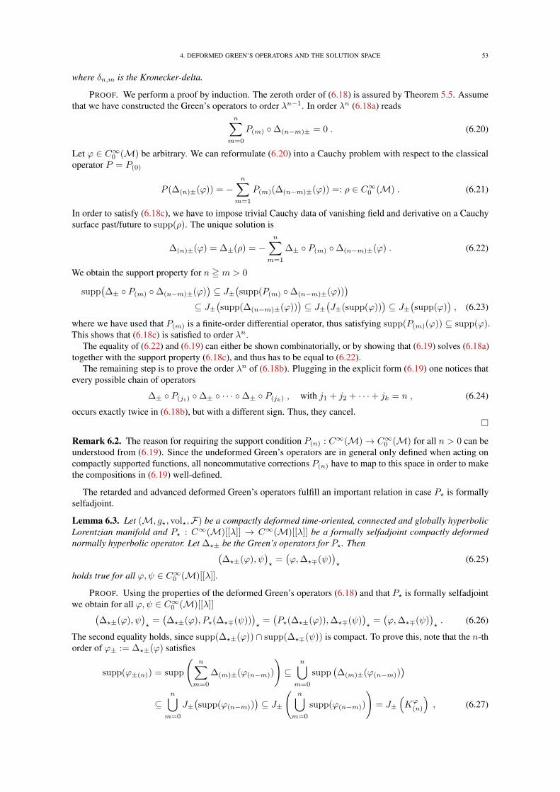
4. DEFORMED GREEN’S OPERATORS AND THE SOLUTION SPACE 53

where δn,m is the Kronecker-delta.

PROOF. We perform a proof by induction. The zeroth order of (6.18) is assured by Theorem 5.5. Assumethat we have constructed the Green’s operators to order λn−1. In order λn (6.18a) reads

n∑m=0

P(m) ∆(n−m)± = 0 . (6.20)

Let ϕ ∈ C∞0 (M) be arbitrary. We can reformulate (6.20) into a Cauchy problem with respect to the classicaloperator P = P(0)

P (∆(n)±(ϕ)) = −n∑

m=1

P(m)(∆(n−m)±(ϕ)) =: ρ ∈ C∞0 (M) . (6.21)

In order to satisfy (6.18c), we have to impose trivial Cauchy data of vanishing field and derivative on a Cauchysurface past/future to supp(ρ). The unique solution is

∆(n)±(ϕ) = ∆±(ρ) = −n∑

m=1

∆± P(m) ∆(n−m)±(ϕ) . (6.22)

We obtain the support property for n = m > 0

supp(∆± P(m) ∆(n−m)±(ϕ)

)⊆ J±

(supp(P(m) ∆(n−m)±(ϕ))

)⊆ J±

(supp(∆(n−m)±(ϕ))

)⊆ J±

(J±(supp(ϕ))

)⊆ J±

(supp(ϕ)

), (6.23)

where we have used that P(m) is a finite-order differential operator, thus satisfying supp(P(m)(ϕ)) ⊆ supp(ϕ).This shows that (6.18c) is satisfied to order λn.

The equality of (6.22) and (6.19) can either be shown combinatorially, or by showing that (6.19) solves (6.18a)together with the support property (6.18c), and thus has to be equal to (6.22).

The remaining step is to prove the order λn of (6.18b). Plugging in the explicit form (6.19) one notices thatevery possible chain of operators

∆± P(j1) ∆± · · · ∆± P(jk) , with j1 + j2 + · · ·+ jk = n , (6.24)

occurs exactly twice in (6.18b), but with a different sign. Thus, they cancel.

Remark 6.2. The reason for requiring the support condition P(n) : C∞(M)→ C∞0 (M) for all n > 0 can beunderstood from (6.19). Since the undeformed Green’s operators are in general only defined when acting oncompactly supported functions, all noncommutative corrections P(n) have to map to this space in order to makethe compositions in (6.19) well-defined.

The retarded and advanced deformed Green’s operators fulfill an important relation in case P? is formallyselfadjoint.

Lemma 6.3. Let (M, g?, vol?,F) be a compactly deformed time-oriented, connected and globally hyperbolicLorentzian manifold and P? : C∞(M)[[λ]] → C∞(M)[[λ]] be a formally selfadjoint compactly deformednormally hyperbolic operator. Let ∆?± be the Green’s operators for P?. Then(

∆?±(ϕ), ψ)?

=(ϕ,∆?∓(ψ)

)?

(6.25)

holds true for all ϕ,ψ ∈ C∞0 (M)[[λ]].

PROOF. Using the properties of the deformed Green’s operators (6.18) and that P? is formally selfadjointwe obtain for all ϕ,ψ ∈ C∞0 (M)[[λ]](

∆?±(ϕ), ψ)?

=(∆?±(ϕ), P?(∆?∓(ψ))

)?

=(P?(∆?±(ϕ)),∆?∓(ψ)

)?

=(ϕ,∆?∓(ψ)

)?. (6.26)

The second equality holds, since supp(∆?±(ϕ)) ∩ supp(∆?∓(ψ)) is compact. To prove this, note that the n-thorder of ϕ± := ∆?±(ϕ) satisfies

supp(ϕ±(n)) = supp

(n∑

m=0

∆(m)±(ϕ(n−m))

)⊆

n⋃m=0

supp(∆(m)±(ϕ(n−m))

)⊆

n⋃m=0

J±(supp(ϕ(n−m))

)⊆ J±

(n⋃

m=0

supp(ϕ(n−m))

)= J±

(Kϕ

(n)

), (6.27)

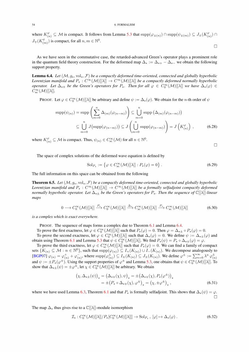
54 6. FORMALISM

where Kϕ(n) ⊆ M is compact. It follows from Lemma 5.3 that supp(ϕ±(n)) ∩ supp(ψ∓(m)) ⊆ J±(Kϕ

(n)) ∩J∓(Kψ

(m)) is compact, for all n,m ∈ N0.

As we have seen in the commutative case, the retarded-advanced Green’s operator plays a prominent rolein the quantum field theory construction. For the deformed map ∆? := ∆?+ −∆?− we obtain the followingsupport property.

Lemma 6.4. Let (M, g?, vol?,F) be a compactly deformed time-oriented, connected and globally hyperbolicLorentzian manifold and P? : C∞(M)[[λ]] → C∞(M)[[λ]] be a compactly deformed normally hyperbolicoperator. Let ∆?± be the Green’s operators for P?. Then for all ϕ ∈ C∞0 (M)[[λ]] we have ∆?(ϕ) ∈C∞sc (M)[[λ]].

PROOF. Let ϕ ∈ C∞0 (M)[[λ]] be arbitrary and define ψ := ∆?(ϕ). We obtain for the n-th order of ψ

supp(ψ(n)) = supp

(n∑

m=0

∆(m)(ϕ(n−m))

)⊆

n⋃m=0

supp(∆(m)(ϕ(n−m))

)⊆

n⋃m=0

J(supp(ϕ(n−m))

)⊆ J

(n⋃

m=0

supp(ϕ(n−m))

)= J

(Kϕ

(n)

), (6.28)

where Kϕ(n) ⊆M is compact. Thus, ψ(n) ∈ C∞sc (M) for all n ∈ N0.

The space of complex solutions of the deformed wave equation is defined by

SolP? :=ϕ ∈ C∞sc (M)[[λ]] : P?(ϕ) = 0

. (6.29)

The full information on this space can be obtained from the following

Theorem 6.5. Let (M, g?, vol?,F) be a compactly deformed time-oriented, connected and globally hyperbolicLorentzian manifold and P? : C∞(M)[[λ]] → C∞(M)[[λ]] be a formally selfadjoint compactly deformednormally hyperbolic operator. Let ∆?± be the Green’s operators for P?. Then the sequence of C[[λ]]-linearmaps

0 −→ C∞0 (M)[[λ]]P?−→ C∞0 (M)[[λ]]

∆?−→ C∞sc (M)[[λ]]P?−→ C∞sc (M)[[λ]] (6.30)

is a complex which is exact everywhere.

PROOF. The sequence of maps forms a complex due to Theorem 6.1 and Lemma 6.4.To prove the first exactness, let ϕ ∈ C∞0 (M)[[λ]] such that P?(ϕ) = 0. Then ϕ = ∆?± P?(ϕ) = 0.To prove the second exactness, let ϕ ∈ C∞0 (M)[[λ]] such that ∆?(ϕ) = 0. We define ψ := ∆?±(ϕ) and

obtain using Theorem 6.1 and Lemma 5.3 that ψ ∈ C∞0 (M)[[λ]]. We find P?(ψ) = P? ∆?±(ϕ) = ϕ.To prove the third exactness, let ϕ ∈ C∞sc (M)[[λ]] such that P?(ϕ) = 0. We can find a family of compact

sets K(n) ⊆ M : n ∈ N0, such that supp(ϕ(n)) ⊆ I+(K(n)) ∪ I−(K(n)). We decompose analogously to[BGP07] ϕ(n) = ϕ+

(n) + ϕ−(n), where supp(ϕ±(n)) ⊆ I±(K(n)) ⊆ J±(K(n)). We define ϕ± :=∑∞n=0 λ

n ϕ±(n)

and ψ := ±P?(ϕ±). Using the support properties of ϕ± and Lemma 5.3, one obtains that ψ ∈ C∞0 (M)[[λ]]. Toshow that ∆?±(ψ) = ±ϕ±, let χ ∈ C∞0 (M)[[λ]] be arbitrary. We obtain(

χ,∆?±(ψ))?

=(∆?∓(χ), ψ

)?

= ±(∆?∓(χ), P?(ϕ

±))?

= ±(P? ∆?∓(χ), ϕ±

)?

=(χ,±ϕ±

)?, (6.31)

where we have used Lemma 6.3, Theorem 6.1 and that P? is formally selfadjoint. This shows that ∆?(ψ) = ϕ.

The map ∆? thus gives rise to a C[[λ]]-module isomorphism

I? : C∞0 (M)[[λ]]/P?[C∞0 (M)[[λ]]]→ SolP? , [ϕ] 7→ ∆?(ϕ) . (6.32)

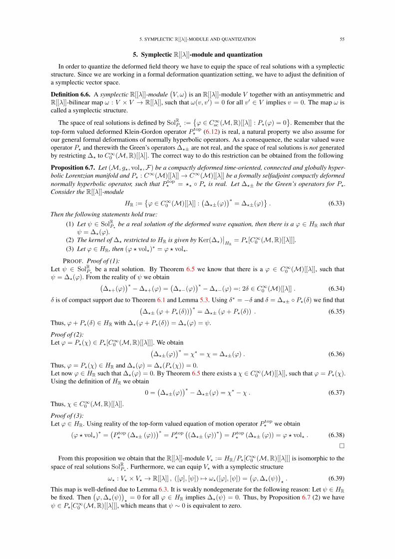
5. SYMPLECTIC R[[λ]]-MODULE AND QUANTIZATION 55

5. Symplectic R[[λ]]-module and quantization

In order to quantize the deformed field theory we have to equip the space of real solutions with a symplecticstructure. Since we are working in a formal deformation quantization setting, we have to adjust the definition ofa symplectic vector space.

Definition 6.6. A symplectic R[[λ]]-module(V, ω

)is an R[[λ]]-module V together with an antisymmetric and

R[[λ]]-bilinear map ω : V × V → R[[λ]], such that ω(v, v′) = 0 for all v′ ∈ V implies v = 0. The map ω iscalled a symplectic structure.

The space of real solutions is defined by SolRP? :=ϕ ∈ C∞sc (M,R)[[λ]] : P?(ϕ) = 0

. Remember that the

top-form valued deformed Klein-Gordon operator P top? (6.12) is real, a natural property we also assume for

our general formal deformations of normally hyperbolic operators. As a consequence, the scalar valued waveoperator P? and therewith the Green’s operators ∆?± are not real, and the space of real solutions is not generatedby restricting ∆? to C∞0 (M,R)[[λ]]. The correct way to do this restriction can be obtained from the following

Proposition 6.7. Let (M, g?, vol?,F) be a compactly deformed time-oriented, connected and globally hyper-bolic Lorentzian manifold and P? : C∞(M)[[λ]]→ C∞(M)[[λ]] be a formally selfadjoint compactly deformednormally hyperbolic operator, such that P top

? = ?? P? is real. Let ∆?± be the Green’s operators for P?.Consider the R[[λ]]-module

HR :=ϕ ∈ C∞0 (M)[[λ]] :

(∆?±(ϕ)

)∗= ∆?±(ϕ)

. (6.33)

Then the following statements hold true:(1) Let ψ ∈ SolRP? be a real solution of the deformed wave equation, then there is a ϕ ∈ HR such that

ψ = ∆?(ϕ).(2) The kernel of ∆? restricted to HR is given by Ker(∆?)

∣∣HR

= P?[C∞0 (M,R)[[λ]]].

(3) Let ϕ ∈ HR, then (ϕ ? vol?)∗ = ϕ ? vol?.

PROOF. Proof of (1):Let ψ ∈ SolRP? be a real solution. By Theorem 6.5 we know that there is a ϕ ∈ C∞0 (M)[[λ]], such thatψ = ∆?(ϕ). From the reality of ψ we obtain(

∆?+(ϕ))∗ −∆?+(ϕ) =

(∆?−(ϕ)

)∗ −∆?−(ϕ) =: 2δ ∈ C∞0 (M)[[λ]] . (6.34)

δ is of compact support due to Theorem 6.1 and Lemma 5.3. Using δ∗ = −δ and δ = ∆?± P?(δ) we find that(∆?± (ϕ+ P?(δ))

)∗= ∆?± (ϕ+ P?(δ)) . (6.35)

Thus, ϕ+ P?(δ) ∈ HR with ∆?(ϕ+ P?(δ)) = ∆?(ϕ) = ψ.

Proof of (2):Let ϕ = P?(χ) ∈ P?[C∞0 (M,R)[[λ]]]. We obtain(

∆?±(ϕ))∗

= χ∗ = χ = ∆?±(ϕ) . (6.36)

Thus, ϕ = P?(χ) ∈ HR and ∆?(ϕ) = ∆?(P?(χ)) = 0.Let now ϕ ∈ HR such that ∆?(ϕ) = 0. By Theorem 6.5 there exists a χ ∈ C∞0 (M)[[λ]], such that ϕ = P?(χ).Using the definition of HR we obtain

0 =(∆?±(ϕ)

)∗ −∆?±(ϕ) = χ∗ − χ . (6.37)

Thus, χ ∈ C∞0 (M,R)[[λ]].

Proof of (3):Let ϕ ∈ HR. Using reality of the top-form valued equation of motion operator P top

? we obtain

(ϕ ? vol?)∗

=(P top? (∆?± (ϕ))

)∗= P top

?

((∆?± (ϕ))

∗)= P top

? (∆?± (ϕ)) = ϕ ? vol? . (6.38)

From this proposition we obtain that the R[[λ]]-module V? := HR/P?[C∞0 (M,R)[[λ]]] is isomorphic to the

space of real solutions SolRP? . Furthermore, we can equip V? with a symplectic structure

ω? : V? × V? → R[[λ]] , ([ϕ], [ψ]) 7→ ω?([ϕ], [ψ]) =(ϕ,∆?(ψ)

)?. (6.39)

This map is well-defined due to Lemma 6.3. It is weakly nondegenerate for the following reason: Let ψ ∈ HRbe fixed. Then

(ϕ,∆?(ψ)

)?

= 0 for all ϕ ∈ HR implies ∆?(ψ) = 0. Thus, by Proposition 6.7 (2) we haveψ ∈ P?[C∞0 (M,R)[[λ]]], which means that ψ ∼ 0 is equivalent to zero.

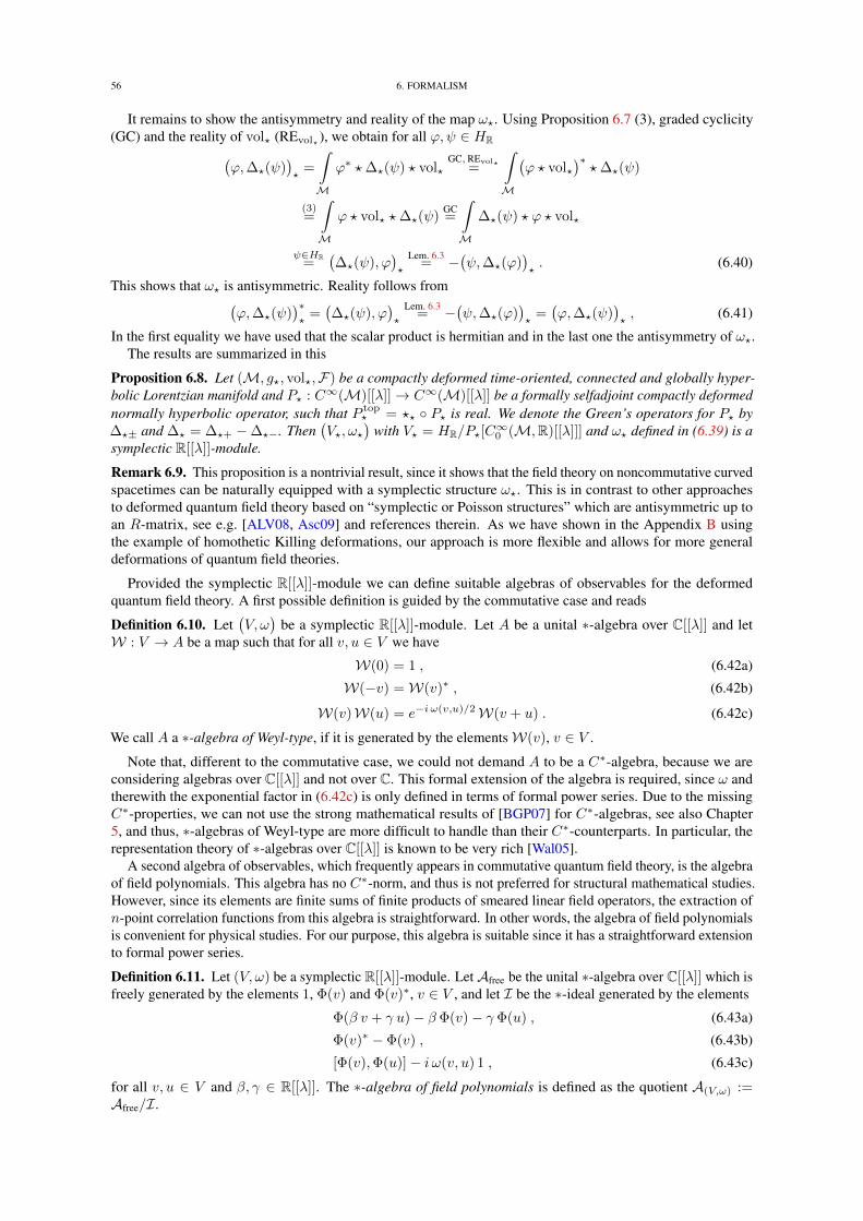
56 6. FORMALISM

It remains to show the antisymmetry and reality of the map ω?. Using Proposition 6.7 (3), graded cyclicity(GC) and the reality of vol? (REvol? ), we obtain for all ϕ,ψ ∈ HR(

ϕ,∆?(ψ))?

=

∫M

ϕ∗ ?∆?(ψ) ? vol?GC,REvol?=

∫M

(ϕ ? vol?

)∗?∆?(ψ)

(3)=

∫M

ϕ ? vol? ?∆?(ψ)GC=

∫M

∆?(ψ) ? ϕ ? vol?

ψ∈HR=

(∆?(ψ), ϕ

)?

Lem. 6.3= −

(ψ,∆?(ϕ)

)?. (6.40)

This shows that ω? is antisymmetric. Reality follows from(ϕ,∆?(ψ)

)∗?

=(∆?(ψ), ϕ

)?

Lem. 6.3= −

(ψ,∆?(ϕ)

)?

=(ϕ,∆?(ψ)

)?, (6.41)

In the first equality we have used that the scalar product is hermitian and in the last one the antisymmetry of ω?.The results are summarized in this

Proposition 6.8. Let (M, g?, vol?,F) be a compactly deformed time-oriented, connected and globally hyper-bolic Lorentzian manifold and P? : C∞(M)[[λ]]→ C∞(M)[[λ]] be a formally selfadjoint compactly deformednormally hyperbolic operator, such that P top

? = ?? P? is real. We denote the Green’s operators for P? by∆?± and ∆? = ∆?+ −∆?−. Then

(V?, ω?

)with V? = HR/P?[C

∞0 (M,R)[[λ]]] and ω? defined in (6.39) is a

symplectic R[[λ]]-module.

Remark 6.9. This proposition is a nontrivial result, since it shows that the field theory on noncommutative curvedspacetimes can be naturally equipped with a symplectic structure ω?. This is in contrast to other approachesto deformed quantum field theory based on “symplectic or Poisson structures” which are antisymmetric up toan R-matrix, see e.g. [ALV08, Asc09] and references therein. As we have shown in the Appendix B usingthe example of homothetic Killing deformations, our approach is more flexible and allows for more generaldeformations of quantum field theories.

Provided the symplectic R[[λ]]-module we can define suitable algebras of observables for the deformedquantum field theory. A first possible definition is guided by the commutative case and reads

Definition 6.10. Let(V, ω

)be a symplectic R[[λ]]-module. Let A be a unital ∗-algebra over C[[λ]] and let

W : V → A be a map such that for all v, u ∈ V we have

W(0) = 1 , (6.42a)

W(−v) =W(v)∗ , (6.42b)

W(v)W(u) = e−i ω(v,u)/2W(v + u) . (6.42c)

We call A a ∗-algebra of Weyl-type, if it is generated by the elementsW(v), v ∈ V .

Note that, different to the commutative case, we could not demand A to be a C∗-algebra, because we areconsidering algebras over C[[λ]] and not over C. This formal extension of the algebra is required, since ω andtherewith the exponential factor in (6.42c) is only defined in terms of formal power series. Due to the missingC∗-properties, we can not use the strong mathematical results of [BGP07] for C∗-algebras, see also Chapter5, and thus, ∗-algebras of Weyl-type are more difficult to handle than their C∗-counterparts. In particular, therepresentation theory of ∗-algebras over C[[λ]] is known to be very rich [Wal05].

A second algebra of observables, which frequently appears in commutative quantum field theory, is the algebraof field polynomials. This algebra has no C∗-norm, and thus is not preferred for structural mathematical studies.However, since its elements are finite sums of finite products of smeared linear field operators, the extraction ofn-point correlation functions from this algebra is straightforward. In other words, the algebra of field polynomialsis convenient for physical studies. For our purpose, this algebra is suitable since it has a straightforward extensionto formal power series.

Definition 6.11. Let (V, ω) be a symplectic R[[λ]]-module. LetAfree be the unital ∗-algebra over C[[λ]] which isfreely generated by the elements 1, Φ(v) and Φ(v)∗, v ∈ V , and let I be the ∗-ideal generated by the elements

Φ(β v + γ u)− β Φ(v)− γ Φ(u) , (6.43a)

Φ(v)∗ − Φ(v) , (6.43b)

[Φ(v),Φ(u)]− i ω(v, u) 1 , (6.43c)

for all v, u ∈ V and β, γ ∈ R[[λ]]. The ∗-algebra of field polynomials is defined as the quotient A(V,ω) :=Afree/I.

6. ALGEBRAIC STATES AND REPRESENTATIONS 57

For notational convenience we do not write the brackets for equivalence classes in A(V,ω) and denote thelinear field operators by Φ(v) ∈ A(V,ω) and not by [Φ(v)].

6. Algebraic states and representations

In order to extract physical observables from the ∗-algebras of observables of the deformed quantum fieldtheory discussed in the previous section we require the notion of an algebraic state. Defining a state on a ∗-algebraA over C[[λ]] to be a positive C-linear map Ω : A→ C turns out to be too naive, since one is immediately facedwith convergence problems or one has to ignore the higher order corrections in λ [Wal05]. A more suitabledefinition is the following

Definition 6.12. An algebraic state (or simply state) on a unital ∗-algebra A over C[[λ]] is a C[[λ]]-linear mapΩ : A→ C[[λ]] such that

Ω(1) = 1 , Ω(a∗a) ≥ 0 , for all a ∈ A . (6.44)

The ordering on R[[λ]] is defined by

R[[λ]] 3 γ =

∞∑n=n0

λn γ(n) > 0 :⇐⇒ γ(n0) > 0 . (6.45)

Ω is called faithful, if Ω(a∗a) = 0 implies a = 0.

A state as defined above associates to each element a ∈ A its expectation value Ω(a) ∈ C[[λ]], which candepend on the deformation parameter λ. Thus, λ can have effects on measurements, which is exactly what wewant.

As argued in [Wal05], suitable spaces on which we can represent ∗-algebras over C[[λ]] are pre-Hilbert spacesover C[[λ]].Definition 6.13.

(a) A C[[λ]]-moduleH with a map 〈·|·〉 : H×H → C[[λ]] is called a pre-Hilbert space over C[[λ]] if1.) 〈·|·〉 is C[[λ]]-linear in the second argument,2.) 〈ψ|φ〉∗ = 〈φ|ψ〉 for all φ, ψ ∈ H,3.) 〈ψ|ψ〉 > 0 for all ψ 6= 0.

(b) Let A be a ∗-algebra over C[[λ]]. A representation of A is a tuple(H, π

), where H is a pre-Hilbert

space over C[[λ]] and π : A→ Lad(H) is a ∗-algebra homomorphism into the algebra of adjoinableoperators onH.A vector |0〉 ∈ H is called cyclic, if π[A]|0〉 = H.A triple

(H, π, |0〉

)is called a cyclic representation ofA, if

(H, π

)is a representation ofA and |0〉 ∈ H

is cyclic.

Similar to the case of unital ∗-algebras over C there is a GNS-construction for unital ∗-algebras over C[[λ]],see [BW98, Wal05] for details. The main result of this construction is summarized in the followingTheorem 6.14 ([BW98, Wal05]).

(i) Let A be a unital ∗-algebra over C[[λ]] and Ω a state on A. Then there exists a cyclic representation(H, π, |0〉

)of A, such that

Ω(a) = 〈0|π(a)|0〉 , for all a ∈ A . (6.46)

The triple(H, π, |0〉

)is called the GNS-representation of Ω.

(ii)(H, π, |0〉

)is unique up to unitary equivalence, i.e. let

(H, π, |0〉

)be another cyclic representation

of A satisfying Ω(a) = 〈0|π(a)|0〉 for all a ∈ A, then there is a unitary U : H → H, such thatUπ(a)U−1 = π(a), for all a ∈ A, and U |0〉 = |0〉.

This theorem shows that, even in the formal power series framework, we can go over from ∗-algebras and statesto a formulation in terms of pre-Hilbert spaces and operators thereon. However, note that there is one essentialdifference: All pre-Hilbert spaces are not equipped (and thus also not complete) with a norm ‖ · ‖ : H → C.Since the usual spectral calculus for operators on Hilbert spaces strongly makes use of this completeness, it isexpected that a spectral calculus in the formal framework will be much more involved.

The last point we want to discuss in this chapter is the choice of an algebraic state for the deformed quantumfield theory. In general, this will be even more ambiguous than the choice of a state for the undeformed quantumfield theory, due to the freedom we get from the formal power series extension. However, as we will show

58 6. FORMALISM

in Chapter 7, there is a ∗-algebra homomorphism from the ∗-algebra of field polynomials of the deformedquantum field theory A(V?,ω?) to the formal power series extension of the ∗-algebra of field polynomials of theundeformed one A(V,ω)[[λ]]. This allows us to induce states from A(V,ω)[[λ]] to A(V?,ω?). There is even thepossibility to induce faithful states from A(V,ω) to faithful states on A(V?,ω?). A faithful state Ω : A(V,ω) → Cfor the undeformed (and unextended) quantum field theory provides a faithful state Ω : A(V,ω)[[λ]]→ C[[λ]] bydefining, for all a ∈ A(V,ω)[[λ]],

Ω(a) :=

∞∑n=0

λn Ω(a(n)) . (6.47)

The map (6.47) is C[[λ]]-linear, satisfies Ω(1) = 1 on A(V,ω)[[λ]], and

Ω(a∗a) =

∞∑n=0

λn∑

m+k=n

Ω(a∗(m) a(k))

= λ2n0 Ω(a∗(n0) a(n0)) +O(λ2n0+1) > 0 , for all a 6= 0 , (6.48)

where n0 ∈ N0 denotes the first nonvanishing term in a =∑∞n=0 λ

n a(n). This state can be pulled-back toA(V?,ω?).

CHAPTER 7

Properties

In this chapter we first reformulate the quantum field theory on noncommutative curved spacetimes presentedin Chapter 6 into a simpler but equivalent setting. This makes in particular reality properties more obvious. Thenwe show that there exist symplectic isomorphisms between the field theory on the deformed and the field theoryon the undeformed spacetime. This eventually leads to ∗-algebra isomorphisms between the corresponding∗-algebras of field polynomials. The mathematical and physical consequences are studied. The results of thischapter appeared in the proceedings article [Sch10] and are influenced by our investigations on special classes ofdeformations, the homothetic Killing deformations [Sch11].

1. Symplectic isomorphism to a simplified formalism

1.1. Wave operators: Let us go back to the deformed wave operator P top? : C∞(M)[[λ]] → ΩN [[λ]]

(6.12). In Chapter 6 we have used the C[[λ]]-module isomorphism

?? : C∞(M)[[λ]]→ ΩN [[λ]] , h 7→ h ? vol? (7.1)

in order to define the scalar valued wave operator

P? := ?−1? P top

? : C∞(M)[[λ]]→ C∞(M)[[λ]] . (7.2)

The resulting operator is formally selfadjoint with respect to the deformed scalar product(ϕ,ψ

)?

=

∫M

ϕ∗ ? ψ ? vol? . (7.3)

However, instead of using ?? we can also employ the undeformed Hodge operator ?g to define a C[[λ]]-moduleisomorphism

?g : C∞(M)[[λ]]→ ΩN [[λ]] , h 7→ h volg =

∞∑n=0

λn h(n) volg . (7.4)

The resulting scalar valued wave operator is

P? := ?−1g P top

? : C∞(M)[[λ]]→ C∞(M)[[λ]] . (7.5)

Since ?? and ?g are isomorphisms, the following equations of motion are equivalent

P?(Φ) = 0 ⇔ P?(Φ) = 0 ⇔ P top? (Φ) = 0 , (7.6)

and therewith also the solution spaces SolP? = SolP? = SolP top?

.We define the C[[λ]]-module automorphism

ι := ?−1g ?? : C∞(M)[[λ]]→ C∞(M)[[λ]] , (7.7)

which relates P? and P? as follows

P? = ι P? . (7.8)

The deformed scalar product (7.3) is related to the undeformed one(ϕ,ψ

)=

∫M

ϕ∗ ψ volg , (7.9)

for all ϕ,ψ ∈ C∞(M)[[λ]] with supp(ϕ) ∩ supp(ψ) compact by(ϕ, ι(ψ)

)=

∫M

ϕ∗ ι(ψ) volg =

∫M

ϕ∗(ψ ? vol?

) GC=

∫M

ϕ∗ ? ψ ? vol? =(ϕ,ψ

)?, (7.10a)

(ι(ϕ), ψ

)=

∫M

(ι(ϕ) volg

)∗ψ =

∫M

(ϕ ? vol?

)∗ψ

GC=

∫M

ϕ∗ ? ψ ? vol? =(ϕ,ψ

)?, (7.10b)

59

60 7. PROPERTIES

where we have used graded cyclicity (GC) (6.8) and the reality of vol?.Let P? : C∞(M)[[λ]]→ C∞(M)[[λ]] be a wave operator which is 1.) a formal deformation of a normally

hyperbolic operator and 2.) formally selfadjoint with respect to the deformed scalar product (7.3). Then we canalways define the wave operator P? := ι P?, which is 1.) a formal deformation of the same normally hyperbolicoperator and 2.) formally selfadjoint with respect to the undeformed scalar product (7.9). The first propertyfollows from ι = id +O(λ) and the second one from a small calculation:(

P?(ϕ), ψ)

=(ι−1 P?(ϕ), ψ

)?

=(P?(ϕ), ψ

)?

=(ϕ, P?(ψ)

)?

=(ϕ, ι P?(ψ)

)=(ϕ, P?(ψ)

), (7.11)

for all ϕ,ψ ∈ C∞(M)[[λ]] with supp(ϕ) ∩ supp(ψ) compact. Vice versa, let P? : C∞(M)[[λ]] →C∞(M)[[λ]] be a wave operator which is 1.) a formal deformation of a normally hyperbolic operator and2.) formally selfadjoint with respect to the undeformed scalar product (7.9). Then we can always define thewave operator P? := ι−1 P?, which is 1.) a formal deformation of the same normally hyperbolic operator and2.) formally selfadjoint with respect to the deformed scalar product (7.3). Furthermore, if (M, g?, vol?,F) isa compactly deformed Lorentzian manifold, then demanding P? or P? to be a compactly deformed normallyhyperbolic operator is equivalent. Thus, studying wave operators of the type P? or P? is equivalent, and therelation is given by P? = ι P?.

The advantage of studying operators of the type P?, compared to the type P?, is that they are real, in case P top?

is real. To see this, note that the isomorphism ?g is real and therewith reality of the top-form valued operatorP top? is equivalent to the reality of P?.

1.2. Green’s operators: For a compactly deformed time-oriented, connected and globally hyperbolicLorentzian manifold (M, g?, vol?,F) we have shown in Theorem 6.1 that there exist unique Green’s operatorsfor all compactly deformed normally hyperbolic operators. Thus, the existence and uniqueness of Green’soperators for both, P? and P?, is guaranteed. We can also derive an explicit map relating the Green’s operators∆?± for P? and the Green’s operators ∆?± for P?. For this consider the following maps

∆?± := ∆?± ι−1 : C∞0 (M)[[λ]]→ C∞(M)[[λ]] . (7.12)

These maps are well-defined, since ι restricts to a C[[λ]]-module automorphism on compactly supported functionsι : C∞0 (M)[[λ]] → C∞0 (M)[[λ]]. We explicitly check the conditions for ∆?± to be Green’s operators for P?(6.18). The first and second condition follow from small calculations

P? ∆?± = ι P? ∆?± ι−1 = ι ι−1 = idC∞0 (M)[[λ]] , (7.13a)

∆?± P?∣∣C∞0 (M)[[λ]]

= ∆?± ι−1 ι P?∣∣C∞0 (M)[[λ]]

= idC∞0 (M)[[λ]] . (7.13b)

To prove the third condition, let ϕ ∈ C∞0 (M) be arbitrary. We obtain

supp(∆(n)±(ϕ)

)= supp

(n∑

m=0

∆(m)±(ι−1(n−m)(ϕ))

)

⊆n⋃

m=0

J±(supp(ι−1

(n−m)(ϕ)))⊆ J±(supp(ϕ)) , (7.13c)

since supp(ι−1(n)(ϕ)) ⊆ supp(ϕ) for all n. Thus, (7.12) are the unique Green’s operators for P?.

We define the retarded-advanced Green’s operator for P? by

∆? := ∆?+ − ∆?− = ∆? ι−1 : C∞0 (M)[[λ]]→ C∞sc (M)[[λ]] . (7.14)

Then the following sequence of C[[λ]]-linear maps is a complex, which is exact everywhere

0 −→ C∞0 (M)[[λ]]P?−→ C∞0 (M)[[λ]]

∆?−→ C∞sc (M)[[λ]]P?−→ C∞sc (M)[[λ]] . (7.15)

Let us make some comments on the proof of this statement. The sequence trivially is a complex, since ∆?± areGreen’s operators for P?. The exactness follows from the exactness of the corresponding complex for P? and∆?, see Theorem 6.5. For completeness, we perform the proof. To show the first exactness, let ϕ ∈ C∞0 (M)[[λ]]

such that P?(ϕ) = ι(P?(ϕ)) = 0. Then due to Theorem 6.5 and the fact that ι is an isomorphism we haveϕ = 0. To show the second exactness, let ϕ ∈ C∞0 (M)[[λ]] such that ∆?(ϕ) = ∆?(ι

−1(ϕ)) = 0. Thenι−1(ϕ) ∈ P?[C∞0 (M)[[λ]]] and ϕ ∈ P?[C∞0 (M)[[λ]]]. To show the third exactness, let ϕ ∈ C∞sc (M)[[λ]] suchthat P?(ϕ) = ι(P?(ϕ)) = 0. Then P?(ϕ) = 0 and ϕ ∈ ∆?[C

∞0 (M)[[λ]]] = ∆?[C

∞0 (M)[[λ]]].

1. SYMPLECTIC ISOMORPHISM TO A SIMPLIFIED FORMALISM 61

The result is that we have the isomorphism

I? : C∞0 (M)[[λ]]/P?[C∞0 (M)[[λ]]]→ SolP? , [ϕ] 7→ ∆?(ϕ) . (7.16)

1.3. Symplectic R[[λ]]-modules: In Proposition 6.7 we have shown that the R[[λ]]-submodule

HR :=ϕ ∈ C∞0 (M)[[λ]] :

(∆?±(ϕ)

)∗= ∆?±(ϕ)

(7.17)

generates by the action of ∆? all real solutions of the wave equation given by P?. As a consequence, theR[[λ]]-module V? = HR/P?[C

∞0 (M,R)[[λ]]] is isomorphic to the space of real solutions SolRP? . We have

equipped V? with the symplectic structure

ω? : V? × V? → R[[λ]] , ([ϕ], [ψ]) 7→(ϕ,∆?(ψ)

)?. (7.18)

For the operator P? the space of real solutions is generated by acting with ∆? on the R[[λ]]-moduleV? := C∞0 (M,R)[[λ]]/P?[C

∞0 (M,R)[[λ]]], more precisely V? is isomorphic to SolR

P?= SolRP? . The natu-

ral symplectic structure on V? reads

ω? : V? × V? → R[[λ]] , ([ϕ], [ψ]) 7→(ϕ, ∆?(ψ)

), (7.19)

where now we use the undeformed scalar product (7.9).There is a symplectic isomorphism between the symplectic R[[λ]]-modules (V?, ω?) and (V?, ω?), which

we are going to construct now. Firstly, note that the map ι provides an R[[λ]]-module isomorphism ι : HR →C∞0 (M,R)[[λ]]. To see this let ϕ ∈ C∞0 (M,R)[[λ]] be arbitrary, then ι−1(ϕ) ∈ HR since(

∆?±(ι−1(ϕ)))∗

=(∆?±(ϕ)

)∗= ∆?±(ϕ) = ∆?±(ι−1(ϕ)) , (7.20)

where we have used that ∆?± are real due to the reality of P?. Let now ϕ ∈ HR be arbitrary, then there is aψ ∈ C∞0 (M)[[λ]], such that ϕ = ι−1(ψ). We find that ψ is real

0 =(∆?±(ϕ)

)∗ −∆?±(ϕ) = ∆?±(ψ∗ − ψ) ⇔ ψ∗ = ψ . (7.21)

The isomorphism ι : HR → C∞0 (M,R)[[λ]] gives rise to an isomorphism between the factor spaces V? and V?,since

ι(ϕ+ P?(ψ)) = ι(ϕ) + P?(ψ) , (7.22)

for all ϕ ∈ HR and ψ ∈ C∞0 (M,R)[[λ]]. Even more, it is a symplectic isomorphism between (V?, ω?) and(V?, ω?), since

ω?([ι(ϕ)], [ι(ψ)]

)=(ι(ϕ), ∆?(ι(ψ))

)=(ϕ,∆?(ψ)

)?

= ω?([ϕ], [ψ]

), (7.23)

for all [ϕ], [ψ] ∈ V?.

1.4. ∗-algebra of field polynomials: The symplectic isomorphism ι : V? → V? leads to an isomorphismbetween the corresponding ∗-algebras of field polynomials A(V?,ω?) and A(V?,ω?), defined in Definition 6.11.This is a consequence of the following

Proposition 7.1. Let (V1, ω1) and (V2, ω2) be two symplectic R[[λ]]-modules and let S : V1 → V2 be asymplectic linear map. Then there exists a ∗-algebra homomorphism S : A(V1,ω1) → A(V2,ω2), such that

S(1) = 1 , (7.24a)

S(Φ1(v)

)= Φ2(S(v)) , (7.24b)

for all v ∈ V1. If S is a symplectic isomorphism then S is a ∗-algebra isomorphism.

PROOF. We construct a ∗-algebra homomorphism σ : Afree1→ Afree2

between the free algebras by definingon the generators

σ(1) = 1 , (7.25a)

σ(Φ1(v)

)= Φ2(S(v)) , (7.25b)

σ(Φ1(v)∗

)= Φ2(S(v))∗ , (7.25c)

62 7. PROPERTIES

for all v ∈ V1, and extending σ toAfree1as a ∗-algebra homomorphism. The ∗-algebra homomorphism σ induces

a ∗-algebra homomorphism S : A(V1,ω1) → A(V2,ω2), since it includes the ∗-ideals (6.43) σ[I1] ⊆ I2, i.e.

σ(Φ1(β v + γ u)− β Φ1(v)− γ Φ1(u)

)= Φ2(β S(v) + γ S(u))− β Φ2(S(v))− γ Φ2(S(u)) , (7.26a)

σ(Φ1(v)∗ − Φ1(v)

)= Φ2(S(v))∗ − Φ2(S(v)) , (7.26b)

σ([Φ1(v),Φ1(u)]− i ω1(v, u) 1

)= [Φ2(S(v)),Φ2(S(u))]− i ω2

(S(v), S(u)

)1 , (7.26c)

are elements of I2 for all v, u ∈ V1 and β, γ ∈ R[[λ]].If S is a symplectic isomorphism, then the map σ is a ∗-algebra isomorphism, which induces a ∗-algebra

isomorphism S : A(V1,ω1) → A(V2,ω2), since σ[I1] = I2.

This proposition has the following consequence: We can equivalently describe a deformed quantum fieldtheory in terms of the ∗-algebra of field polynomials A(V?,ω?) or A(V?,ω?). However, the physical interpretationhas to be adapted properly. Due to the modified reality property of the R[[λ]]-module HR, see Proposition 6.7,we should interpret the generators Φ?([ϕ]) ofA(V?,ω?) as smeared field operators “Φ?([ϕ]) =

∫MΦ? ?ϕ? vol?”.

The property (ϕ ? vol?)∗ = ϕ ? vol?, for all ϕ ∈ HR, implies that formally Φ?([ϕ])∗ = Φ?([ϕ]). On the other

hand, since V? is based on the space of real compactly supported functions C∞0 (M,R)[[λ]], the correspondinggenerators Φ?([ϕ]) of A(V?,ω?) should be interpreted as smeared field operators “Φ?([ϕ]) =

∫M Φ? ϕ volg”

without ?-products.

2. Symplectic isomorphisms to commutative field theory

In this section we provide a theorem showing that the deformed symplectic R[[λ]]-module (V?, ω?) isisomorphic, via a symplectic isomorphism, to the formal power series extension of the undeformed symplecticvector space1 (V [[λ]], ω), where V := C∞0 (M,R)/P [C∞0 (M,R)] and

ω : V [[λ]]× V [[λ]]→ R[[λ]] , ([ϕ], [ψ]) 7→ ω([ϕ], [ψ]) =(ϕ,∆(ψ)

). (7.27)

Here P = P?|λ=0 is the undeformed wave operator and ∆ = ∆?|λ=0 is the corresponding undeformedretarded-advanced Green’s operator. For the undeformed field theory we have the isomorphism

I : C∞0 (M)[[λ]]/P [C∞0 (M)[[λ]]]→ SolP , [ϕ] 7→ ∆(ϕ) , (7.28)

which leads to an isomorphism V [[λ]] ' SolRP .

Lemma 7.2. Let (M, g?, vol?,F) be a compactly deformed time-oriented, connected and globally hyperbolicLorentzian manifold and P? : C∞(M)[[λ]]→ C∞(M)[[λ]] be a real compactly deformed normally hyperbolicoperator. Let ∆?± be the Green’s operators for P?. Then the maps T± : SolR

P?→ SolRP defined by

T± := idC∞sc (M)[[λ]] + t± = idC∞sc (M)[[λ]] + ∆± ∞∑n=1

λn P(n) (7.29)

are R[[λ]]-module isomorphisms.

PROOF. The compositions ∆± P(n) are well-defined due to the support condition on P(n), n > 0.Additionally, the maps ∆± P(n) are real for all n > 0. The composition of P and T± is given by

P T± = P + P ∆± ∞∑n=1

λn P(n) = P +

∞∑n=1

λn P(n) =

∞∑n=0

λn P(n) = P? , (7.30)

where we have used that P ∆± = idC∞0 (M)[[λ]]. Thus, for all Φ ∈ SolRP?

we have T±(Φ) ∈ SolRP .The inverse of T± is constructed by the geometric series

T−1± =

(idC∞sc (M)[[λ]] + t±

)−1=

∞∑m=0

(−t±)m (6.19)

= idC∞sc (M)[[λ]] − ∆?± ∞∑n=1

λn P(n) (7.31)

1 Note that C∞0 (M,R)[[λ]]/P [C∞0 (M,R)[[λ]]] ' V [[λ]] via the map C∞0 (M,R)[[λ]]/P [C∞0 (M,R)[[λ]]]→ V [[λ]] , [ϕ] 7→∑∞n=0 λ

n [ϕ(n)] . This natural identification will be used frequently throughout this section, without explicitly denoting the correspondingmap by some symbol.

2. SYMPLECTIC ISOMORPHISMS TO COMMUTATIVE FIELD THEORY 63

and satisfies

P? T−1± = P? − P? ∆?±

∞∑n=1

λn P(n) = P? −∞∑n=1

λn P(n) = P , (7.32)

where we have used that P? ∆?± = idC∞0 (M)[[λ]]. Thus, for all Φ ∈ SolRP we have T−1± (Φ) ∈ SolR

P?.

It turns out that in general T+ and T− differ. To see this let Φ ∈ SolRP?

be arbitrary. Then there is a

ϕ ∈ C∞0 (M,R)[[λ]], such that Φ = ∆?(ϕ). We obtain

T+(Φ)− T−(Φ) = ∆

( ∞∑n=1

λn P(n)

(∆?(ϕ)

))= −∆

(P(

∆?(ϕ)))

. (7.33)

The difference between T+ and T− is thus related to the operator ∆ P ∆?. Notice that this operator is notzero in general, since the relation ∆ P = 0 just holds when acting on functions of compact support, while ∆?

maps to functions of noncompact support. To be more explicit we expand the operator ∆ P ∆? to first orderin λ by using (6.19) and find

∆ P ∆? = ∆ P (∆− λ(∆+ P(1) ∆+ −∆− P(1) ∆−)

)+O(λ2)

= −λ∆ P(1) ∆ +O(λ2) . (7.34)

Since P(1) comes from the choice of deformation, while ∆ describes the commutative dynamics, these operatorsare independent and ∆ P ∆? in general does not vanish.

Remark 7.3. The maps T± can be interpreted as retarded/advanced isomorphisms, since they depend on theretarded/advanced Green’s operators. Due to the support property of ∆± and the support condition on P(n),n > 0, we obtain order by order in λ that T±(Φ) is equal to Φ for sufficiently small/large times, i.e. for t→ ∓∞.

Employing the isomorphisms T±, the isomorphism I? (7.16) and its commutative counterpart I (7.28), weobtain the R[[λ]]-module isomorphisms T± := I−1 T± I? : V? → V [[λ]]. We can map the deformedsymplectic R[[λ]]-module (V?, ω?), via a symplectic isomorphism, to the symplectic R[[λ]]-module (V [[λ]], ω?),where by definition

ω?([ϕ], [ψ]

):= ω?

(T−1±([ϕ]),T−1±([ψ])), (7.35)

for all [ϕ], [ψ] ∈ V [[λ]]. This expression can be simplified and we obtain

ω?([ϕ], [ψ]

)=(T−1± ([ϕ]), ∆?

(T−1± ([ψ])

))=(T−1± ([ϕ]), T−1

±(∆(ψ)

))=(T−1†±(T−1± ([ϕ])

),∆(ψ)

)= −

(∆(T−1†±(T−1± ([ϕ])

)), ψ), (7.36)

where we have used the adjoint map

T−1†± = idC∞0 (M)[[λ]] −

∞∑n=1

λn P(n) ∆?∓ (7.37)

and that ∆ is antihermitian. Defining the map ∆? : C∞0 (M)[[λ]]→ SolP by

∆? := ∆ T−1†± I−1

? T−1± ∆ , (7.38)

we have for all [ϕ], [ψ] ∈ V [[λ]]

ω?([ϕ], [ψ]

)=(ϕ, ∆?(ψ)

). (7.39)

Analogously to (7.28) and (7.16) we define the isomorphism

I? : C∞0 (M)[[λ]]/P [C∞0 (M)[[λ]]]→ SolP , [ϕ] 7→ ∆?(ϕ) , (7.40)

which leads to an isomorphism V [[λ]] ' SolRP . We obtain the following

64 7. PROPERTIES

Theorem 7.4. The map S : V [[λ]]→ V [[λ]] defined by S =∞∑n=0

λnS(n), where

S(0) = idV , (7.41a)

S(1) =1

2I−1 I(1) , (7.41b)

S(n) =1

2

(I−1 I(n) −

n−1∑m=1

S(m) S(n−m)

), ∀n ≥ 2 , (7.41c)

provides a symplectic isomorphism between (V [[λ]], ω?) and (V [[λ]], ω), i.e. for all v, u ∈ V [[λ]] we haveω?(v, u) = ω(S(v),S(u)).

PROOF. The map S is invertible, since it is a formal deformation of the identity map. Let v, u ∈ V [[λ]] bearbitrary. We obtain

ω(S(v),S(u)) =

∞∑n=0

λn∑

m+k+i+j=n

ω(S(m)(v(k)), S(i)(u(j))

)=

∞∑n=0

λn∑

k+j+l=n

∑m+i=l

ω(S(m)(v(k)), S(i)(u(j))

). (7.42)

Note that for all v, u ∈ V we have ω(v, S(0)(u)) = ω(S(0)(v), u) (trivially) and

ω(v, S(1)(u)) =1

2ω(1)(v, u) = −1

2ω(1)(u, v) = ω(S(1)(v), u) . (7.43)

By induction it follows that ω(v, S(n)(u)) = ω(S(n)(v), u) for all n ≥ 0.Using this, the inner sum of (7.42) reads

∑m+i=l

ω(S(m)(v(k)), S(i)(u)(j)) = ω

(v(k),

l∑m=0

S(m) S(l−m)(u(j))

). (7.44)

It remains to simplify the map∑lm=0 S(m) S(l−m). For l = 0 this is simply the identity map and for l = 1 it

reads 2S(1) = I−1 I(1). For l ≥ 2 we find

l∑m=0

S(m) S(l−m) = 2S(l) +

l−1∑m=1

S(m) S(l−m) = I−1 I(l) . (7.45)

Thus, (7.42) reads

ω(S(v),S(u)) =

∞∑n=0

λn∑

k+j+l=n

ω(v(k), I−1 I(l)(u(j))

)= ω?(v, u) . (7.46)

As a direct consequence we obtain

Corollary 7.5. The maps S± := S T± : V? → V [[λ]] are symplectic isomorphisms between (V?, ω?) and(V [[λ]], ω), i.e. ω

(S±(v), S±(u)

)= ω?

(v, u)

for all v, u ∈ V?.Moreover, the maps S± := S± ι : V? → V [[λ]] are symplectic isomorphisms between (V?, ω?) and (V [[λ]], ω).

3. Consequences of the symplectic isomorphisms

We study the consequences of the symplectic isomorphisms S± : V? → V [[λ]]. Analogous results hold truefor the symplectic isomorphisms S± : V? → V [[λ]].

3.1. ∗-algebra of field polynomials: Consider the ∗-algebras of field polynomialsA(V?,ω?) andA(V [[λ]],ω)

of the deformed and undeformed quantum field theory, respectively. From Proposition 7.1 we immediately obtain

Corollary 7.6. There exist ∗-algebra isomorphisms S± : A(V?,ω?) → A(V [[λ]],ω).

3. CONSEQUENCES OF THE SYMPLECTIC ISOMORPHISMS 65

This means that we can mathematically describe the quantum field theory on noncommutative curvedspacetimes by a formal power series extension of the corresponding quantum field theory on commutativecurved spacetimes. However, the physical interpretation has to be adapted properly: If we want to probe thedeformed quantum field theory with a set of smearing functions [ϕi] in order to extract physical observables(e.g. correlation functions) we have to probe the corresponding commutative quantum field theory with a differentset of smearing functions S±([ϕi]) in order to obtain the same result. We will come back to this point whenwe discuss n-point functions.

There is a mathematical subtlety at this point: Instead of the algebra A(V [[λ]],ω) for the undeformed quantumfield theory we could also consider the algebra A(V,ω)[[λ]], where we first construct the ∗-algebra of fieldpolynomials over C and afterwards extend by formal power series. There is a natural identification of elements inA(V [[λ]],ω) with elements in A(V,ω)[[λ]] given by regarding the generators Φ(v), v ∈ V [[λ]], as formal powerseries Φ(v) =

∑∞n=0 λ

n Φ(v(n)), where on the right hand side Φ(v(n)), v(n) ∈ V , denote the generators ofA(V,ω). However, this identification just provides a ∗-algebra homomorphism A(V [[λ]],ω) → A(V,ω)[[λ]], whichis no isomorphism in general. Employing methods from the Appendix A, we obtain that A(V,ω)[[λ]] is the λ-adiccompletion of A(V [[λ]],ω). For the deformed quantum field theory this means that there is in addition to the∗-algebra isomorphism A(V?,ω?) ' A(V [[λ]],ω) also a ∗-algebra homomorphism A(V?,ω?) → A(V,ω)[[λ]], whichis not necessarily invertible.

3.2. Symplectic automorphisms: An important class of symmetries of quantum field theories are thosewhich are induced by symplectic automorphisms of the corresponding symplectic R[[λ]]-module.

Definition 7.7. Let (V, ω) be a symplectic R[[λ]]-module. A map α ∈ EndR[[λ]](V ) is called a symplecticautomorphism, if it is invertible and if ω(α(v), α(u)) = ω(v, u), for all v, u ∈ V . The set G(V,ω) ⊆ EndR[[λ]](V )of all symplectic automorphisms forms a group under the usual composition of endomorphisms. This group iscalled the group of symplectic automorphisms.

Due to the symplectic isomorphisms S± : V? → V [[λ]] we obtain the following

Corollary 7.8. There exist group isomorphisms S±G : G(V [[λ]],ω) → G(V?,ω?) , α 7→ S−1± α S±.

The group of symplectic automorphisms of a symplectic R[[λ]]-module (V, ω) can be represented on its∗-algebra of field polynomials by defining on the generators, for all α ∈ G(V,ω),

α(1) = 1 , α(Φ(v)

)= Φ(α(v)) , for all v ∈ V , (7.47)

and extending to A(V,ω) as ∗-algebra homomorphisms.

Example 7.9. Let (M, g?, vol?,F) be a compactly deformed time-oriented, connected and globally hyperbolicLorentzian manifold and P? : C∞(M)[[λ]]→ C∞(M)[[λ]] be the deformed Klein-Gordon operator. Assumethat the underlying classical Lorentzian manifold (M, g) has a group Giso of isometries. Due to the Giso-invariance of the classical Klein-Gordon operator and the classical Green’s operators we have Giso ⊆ G(V [[λ]],ω),where the action ofGiso on V [[λ]] is given by the geometric action. Corollary 7.8 states that the deformed quantumfield theory A(V?,ω?) enjoys the same transformations as symplectic automorphisms, i.e. Giso ⊆ G(V?,ω?), notdependent on details of the deformation. The action is given by α? := S−1

± α S± and it is in general differentto the geometric action. Thus, the deformation does not break isometries of the undeformed quantum field theory,but replaces geometric symmetries by nongeometric ones.

3.3. Algebraic states: Due to the symplectic isomorphisms S± : V? → V [[λ]] the space of algebraic stateson A(V?,ω?) and A(V [[λ]],ω) can be related in a precise way. To explain this, we require the following

Lemma 7.10. Let A1 and A2 be two unital ∗-algebras over C[[λ]] and κ : A1 → A2 be a ∗-algebra homomor-phism. Then each state Ω2 on A2 induces a state Ω1 on A1 by defining

Ω1(a) := Ω2(κ(a)) , (7.48)

for all a ∈ A1.

PROOF. Ω1 : A1 → C[[λ]] is a C[[λ]]-linear map. We have Ω1(1) = Ω2(κ(1)) = Ω2(1) = 1 and

Ω1(a∗a) = Ω2

(κ(a∗a)

)= Ω2

((κ(a))∗κ(a)

)≥ 0 , (7.49)

for all a ∈ A1.

The state Ω1 defined above is called the pull-back of Ω2 under the ∗-algebra homomorphism κ. Note thatfor ∗-algebra isomorphisms κ : A1 → A2 there is bijection between the states on A1 and A2. We immediatelyobtain from Corollary 7.6 and the Lemma above

66 7. PROPERTIES

Corollary 7.11. The ∗-algebra isomorphisms S± : A(V?,ω?) → A(V [[λ]],ω) provide bijections between thestates on A(V?,ω?) and A(V [[λ]],ω). G(V [[λ]],ω)-symmetric states are pulled-back to G(V?,ω?)-symmetric states,and vice versa.

As discussed before in Chapter 6, Section 6, we can induce faithful states on A(V,ω)[[λ]] from faithful stateson the undeformed and unextended quantum field theory A(V,ω). The ∗-algebra homomorphism A(V?,ω?) →A(V,ω)[[λ]] allows us to pull-back also these states on the deformed quantum field theory.

3.4. n-point functions: We now focus on n-point functions in the deformed and undeformed quantum fieldtheory. Let Ω be an algebraic state on A(V [[λ]],ω). We define the n-point correlation functions by

Ωn : C∞0 (M,R)[[λ]]×n → C[[λ]] , (ϕ1, . . . , ϕn) 7→ Ω(Φ([ϕ1]) · · ·Φ([ϕn])

). (7.50)

Using the ∗-algebra isomorphism S± we can pull-back the state Ω to a state Ω? on the deformed quantum fieldtheory A(V?,ω?). The deformed n-point correlation functions can be expressed in terms of the undeformed onesvia

Ω?n : H×nR → C[[λ]] , (ϕ1, . . . , ϕn) 7→ Ω(Φ(S±([ϕ1])) · · ·Φ(S±([ϕn]))

). (7.51)

Note that Ω?n is defined on HR, such that we can not directly compare it to the undeformed correlationfunctions Ωn, acting on compactly supported real functions. This is due to the different smearing interpretationwe have for the generators Φ([ϕ]) of A(V [[λ]],ω) and Φ?([ϕ]) of A(V?,ω?) (the latter ones are smeared with?-products). Composing Ω?n with the isomorphism

(ι−1)×n

: C∞0 (M,R)[[λ]]×n → H×nR we obtain thecorrelation functions for the quantum field theory A(V?,ω?)

Ω?n := Ω?n (ι−1)×n

: C∞0 (M,R)[[λ]]×n → C[[λ]] ,

(ϕ1, . . . , ϕn) 7→ Ω(Φ(S±([ϕ1])) · · ·Φ(S±([ϕn])

). (7.52)

Since both, Ωn and Ω?n, are maps on real functions of compact support, we can compare them. Due to the mapsS±, the undeformed and deformed correlation functions evaluated on the same functions do not agree

Ωn(ϕ1, . . . , ϕn) 6= Ω?n(ϕ1, . . . , ϕn) . (7.53)

Because the functions ϕi which localize the correlation functions are fixed by details of the experimental setup,using the same apparatus we could in principle distinguish between the deformed and undeformed quantumfield theory in the state Ω? and Ω, respectively. For example, in cosmology the usual prescription to extract theprimordial power spectrum is to evaluate the 2-point correlation function, regarded as a distribution kernel, onequal-time hypersurfaces. If we apply the same prescription to the deformed quantum field theory we obtain

Ω2(x1, x2) 6= Ω?2(x1, x2) . (7.54)

This discussion shows that the deformed quantum field theory in the induced state Ω? is physically inequivalentto the undeformed quantum field theory in the state Ω. It remains to exclude the possibility that there is a differentstate Ω′ of the undeformed quantum field theory such that all n-point functions Ω′n in this state coincide withthe deformed n-point functions Ω?n. If this would be the case, then we would in particular have, for allϕ,ψ ∈ C∞0 (M,R)[[λ]],

Ω?2(ϕ,ψ) = Ω′2(ϕ,ψ) . (7.55)

This is, however, inconsistent with the canonical commutation relations, since for a nontrivial S±

Ω?2(ϕ,ψ)− Ω?2(ψ,ϕ) = ω?(ϕ,ψ) 6= ω(ϕ,ψ) = Ω′2(ϕ,ψ)− Ω′2(ψ,ϕ) . (7.56)

This proves that the deformation can lead to new physical effects, even though the underlying algebras ofobservables are isomorphic, i.e. mathematically equivalent.

CHAPTER 8

Applications

We now study explicit examples of deformed classical and quantum field theories. This chapter is mainlybased on the articles [SU10a, SU10b, Sch11].

1. Examples of deformed wave operators

For discussing explicit examples of deformed wave operators it is convenient to rewrite the deformed actionfunctional (6.9) for the real scalar field Φ in terms of local bases.

Firstly, let us use a generic local coordinate basis ∂µ ∈ Ξ[[λ]] : µ = 1, . . . , N for the vector fields Ξ[[λ]].We define the ?-dual basis of one-forms dxµ? ∈ Ω1[[λ]] : µ = 1, . . . , N by 〈∂µ, dxν?〉? = δνµ. As a consequenceof F = 1⊗ 1 +O(λ) we obtain dxµ? = dxµ +O(λ), for all µ, where dxµ is the undeformed dual basis of∂µ defined by 〈∂µ, dxν〉 = δνµ. The differential d acting on functions corresponds to the undeformed one.Thus, we have in the undeformed basis dϕ = dxµ ∂µϕ, for all ϕ ∈ C∞(M)[[λ]]. Since dxµ? is also a basis ofΩ1[[λ]] we can find for all ϕ coefficient functions ∂?µϕ ∈ C∞(M)[[λ]], such that dϕ = dxµ ∂µϕ = dxµ? ?∂?µϕ.Evaluating the ?-products and dxµ? on the right hand side of this expression we can construct the deformedpartial derivatives ∂?µ order by order in λ. The inverse metric field can be expressed in the local basis asg−1? = ∂µ ⊗A? g

µν? ? ∂ν . The involution ∗ on Ξ[[λ]] satisfies ∂∗µ = −∂µ [ADMW06]. From this, the reality of

the twist and the hermiticity of g−1? we obtain for the coefficient functions(

gµν?)∗

= gνµ? . (8.1)

Furthermore, for real functions ϕ we have

dϕ = −(dϕ)∗ = −(dxµ? ? ∂?µϕ)∗ = −(∂?µϕ

)∗? dxµ∗? . (8.2)

With this we can express the kinetic term in the deformed action (6.9) in terms of the local coordinate basis

〈〈dΦ, g−1? 〉?,dΦ〉? = −

(∂?µΦ

)∗? 〈dxµ∗? , ∂ν〉? ? gνρ? ? 〈∂ρ, dxσ? 〉? ? ∂?σΦ

= −(∂?µΦ

)∗? 〈∂∗ν , dxµ? 〉∗? ? gνρ? ? ∂?ρΦ

∂∗ν=−∂ν=

(∂?µΦ

)∗? gµρ? ? ∂?ρΦ . (8.3)

The deformed action (6.9) then reads in the basis

S?[Φ] = −1

2

∫M

((∂?µΦ

)∗? gµν? ? ∂?νΦ +M2 Φ ? Φ

)? vol? , (8.4)

where we could also express the volume form in terms of the basis, vol? = γ? ? dx1? ∧? · · · ∧? dxN? . By classical

correspondence we know that γ? =√−det(gµν) +O(λ). The equation of motion in the basis can be derived

from (8.4) order by order in λ via multiple integrations by parts. Even though the deformed action (8.4) lookspretty familiar and simple, there are two issues which in general complicate the application of this formula: Onerequires the inverse metric field gµν? in the ?-basis and one has to determine the deformed partial derivatives ∂?µ,which are higher differential operators, to all orders in λ recursively.

As we have observed in Chapter 3, Section 1, the formulae of noncommutative differential geometry simplifywhen we use a nice basis. As a reminder, a nice basis ea ∈ Ξ[[λ]] : a = 1, . . . , N satisfies the conditions[ea, eb] = 0 and [F, ea] = 0, for all a, b, where F ⊆ Ξ is the Lie subalgebra generating the twist, i.e. F ∈(UF⊗ UF)[[λ]]. For a large class of abelian twists, the nonexotic ones, such a basis exists for opens U ⊆Maround almost all points p ∈M [AC10]. Let us now derive an expression for the deformed action (6.9) in thenice basis ea and its dual θa, which is also F-invariant LF(θa) = 0. For the inverse metric field we canwrite g−1

? = ea⊗A? gab? ?eb = ea⊗A gab? eb. The differential of a function ϕ reads dϕ = θa ?ea(ϕ) = θa ea(ϕ),where ea(·) denotes the vector field action (Lie derivative) of ea on functions. The basis expression for the kineticterm is

〈〈dΦ, g−1? 〉?,dΦ〉? = ea(Φ) ? 〈θa, eb〉? ? gbc? ? 〈ec, θd〉? ? ed(Φ) = ea(Φ) ? gab? ? eb(Φ) . (8.5)

67

68 8. APPLICATIONS

Plugging this into the action yields

S?[Φ] = −1

2

∫M

((ea(Φ) ? gab? ? eb(Φ) +M2 Φ ? Φ

)? γ? ? cnt , (8.6)

where cnt = θ1 ∧? · · · ∧? θN = θ1 ∧ · · · ∧ θN is the basis top-form satisfying LF(cnt) = 0 and γ? is thevolume factor determined by vol? = γ? ? cnt = γ? cnt. The obvious advantage of (8.6) compared to (8.4) is thatno higher differential operators ∂?µ appear. Using graded cyclicity (6.8), integration by parts, F-invariance of cntand Lea(cnt) = 0, for all a, we can easily calculate the equation of motion operator by varying (8.6) and obtain

P top? (Φ) =

1

2

(ea(gab? ? eb(Φ) ? γ?

)+ ea

(γ? ? eb(Φ) ? gba?

)−M2

(Φ ? γ? + γ? ? Φ

))? cnt . (8.7)

The scalar valued equation of motion operator is given by

P?(Φ) =1

2

(ea(gab? ? eb(Φ) ? γ?

)+ ea

(γ? ? eb(Φ) ? gba?

)−M2

(Φ ? γ? + γ? ? Φ

))? γ−1?

? , (8.8)

where γ−1?? is the ?-inverse of γ?, i.e. γ? ? γ−1?

? = γ−1?? ? γ? = 1. For completeness, the real equation of motion

operator P? reads

P?(Φ) =1

2

(ea(gab? ? eb(Φ) ? γ?

)+ ea

(γ? ? eb(Φ) ? gba?

)−M2

(Φ ? γ? + γ? ? Φ

))γ−1 , (8.9)

where γ−1 is the inverse volume factor of the undeformed volume form volg = γ cnt.We are now going to derive explicit examples of these operators, where the twist is given by an abelian twist

F = exp

(− iλ

2ΘαβXα ⊗Xβ

), (8.10)

with [Xα, Xβ ] = 0 for all α, β and Θ canonical.

1.1. Noncommutative Minkowski spacetimes: The simplest example is to consider the 4-dimensionalMinkowski spacetime, i.e.M = R4 with metric g−1

? = g−1 = ∂µ ⊗A gµν∂ν , where in Cartesian coordinatesgµν = diag(−1, 1, 1, 1)µν . The volume form is taken to be the classical one vol? = volg = dt∧dx1∧dx2∧dx3.

If we deform this spacetime with the Moyal-Weyl twist, the nice basis and coordinate basis chosen abovecoincide and we find for the equation of motion operators (8.8) and (8.9)

P?(Φ) = P?(Φ) = P (Φ) = gµν∂µ∂νΦ−M2 Φ . (8.11)

Thus, the wave operator for the Moyal-Weyl deformed Minkowski spacetime is undeformed, which is a well-known result.

Consider now the abelian twist (8.10) with X1 = r∂r and X2 = ∂t, where r is the spatial radius coordinate.The resulting commutation relations are [t ?, r] = −i λ r, i.e. we are dealing with a κ-deformed Minkowskispacetime. Note that since X2 is a Killing vector field, the undeformed metric field solves the noncommutativevacuum Einstein equations exactly. A nice basis for this deformation is given by

e1 = ∂t , e2 = r∂r , e3 = ∂ζ , e4 = ∂φ , (8.12)

where ζ is the polar and φ is the azimuthal angle. The dual basis is

θ1 = dt , θ2 =dr

r, θ3 = dζ , θ4 = dφ . (8.13)

The inverse metric field in this basis reads gab? = diag(−1, r−2, r−2, (r sin ζ)−2

)aband the volume factor is

γ? = γ = r3 sin ζ. Note that γ−1?? = γ−1 = r−3 (sin ζ)−1. Evaluating all ?-products in the equation of motion

operator (8.8) we obtain

P?(Φ) = −1

2

(1 + ei3λ∂t

)(∂2t +M2

)Φ +

1

2

(e−iλ∂t + ei4λ∂t

)4 Φ , (8.14)

where4 is the spatial Laplacian. The tilded operator reads

P?(Φ) = − cosh

(3λ

2i∂t

)(∂2t +M2

)Φ + cosh

(5λ

2i∂t

)4 Φ . (8.15)

For this derivation the following identities are useful

(rn) ? h = rn einλ2 ∂th , h ? (rn) = rn e−

inλ2 ∂th , (8.16)

for all n ∈ Z and h ∈ C∞(M)[[λ]].Thus, we obtain a nontrivial wave operator for the scalar field on the deformed Minkowski spacetime. The

second order corrections to the Green’s operators for this model are calculated in the Appendix C.

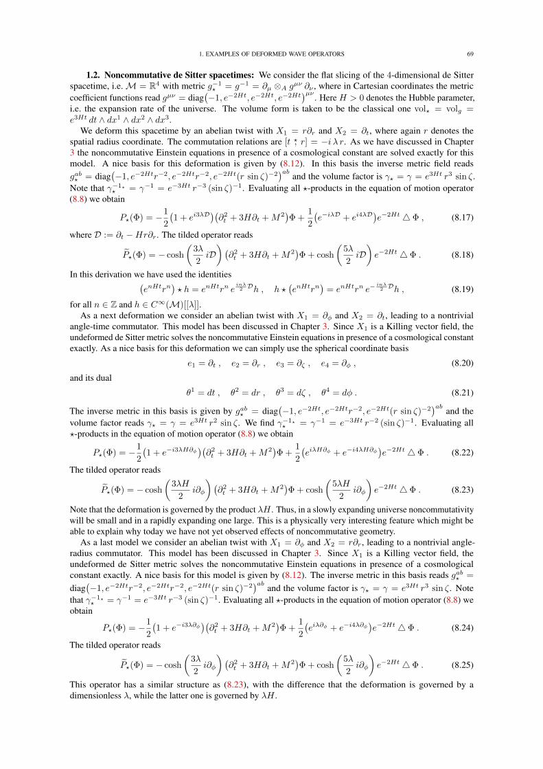
1. EXAMPLES OF DEFORMED WAVE OPERATORS 69

1.2. Noncommutative de Sitter spacetimes: We consider the flat slicing of the 4-dimensional de Sitterspacetime, i.e.M = R4 with metric g−1

? = g−1 = ∂µ ⊗A gµν ∂ν , where in Cartesian coordinates the metriccoefficient functions read gµν = diag

(−1, e−2Ht, e−2Ht, e−2Ht

)µν. Here H > 0 denotes the Hubble parameter,

i.e. the expansion rate of the universe. The volume form is taken to be the classical one vol? = volg =e3Ht dt ∧ dx1 ∧ dx2 ∧ dx3.

We deform this spacetime by an abelian twist with X1 = r∂r and X2 = ∂t, where again r denotes thespatial radius coordinate. The commutation relations are [t ?, r] = −i λ r. As we have discussed in Chapter3 the noncommutative Einstein equations in presence of a cosmological constant are solved exactly for thismodel. A nice basis for this deformation is given by (8.12). In this basis the inverse metric field readsgab? = diag

(−1, e−2Htr−2, e−2Htr−2, e−2Ht(r sin ζ)−2

)aband the volume factor is γ? = γ = e3Ht r3 sin ζ.

Note that γ−1?? = γ−1 = e−3Ht r−3 (sin ζ)−1. Evaluating all ?-products in the equation of motion operator

(8.8) we obtain

P?(Φ) = −1

2

(1 + ei3λD

)(∂2t + 3H∂t +M2

)Φ +

1

2

(e−iλD + ei4λD

)e−2Ht 4 Φ , (8.17)

where D := ∂t −Hr∂r. The tilded operator reads

P?(Φ) = − cosh

(3λ

2iD)(

∂2t + 3H∂t +M2

)Φ + cosh

(5λ

2iD)e−2Ht 4 Φ . (8.18)

In this derivation we have used the identities(enHtrn

)? h = enHtrn e

inλ2 Dh , h ?

(enHtrn

)= enHtrn e−

inλ2 Dh , (8.19)

for all n ∈ Z and h ∈ C∞(M)[[λ]].As a next deformation we consider an abelian twist with X1 = ∂φ and X2 = ∂t, leading to a nontrivial

angle-time commutator. This model has been discussed in Chapter 3. Since X1 is a Killing vector field, theundeformed de Sitter metric solves the noncommutative Einstein equations in presence of a cosmological constantexactly. As a nice basis for this deformation we can simply use the spherical coordinate basis

e1 = ∂t , e2 = ∂r , e3 = ∂ζ , e4 = ∂φ , (8.20)

and its dual

θ1 = dt , θ2 = dr , θ3 = dζ , θ4 = dφ . (8.21)

The inverse metric in this basis is given by gab? = diag(−1, e−2Ht, e−2Htr−2, e−2Ht(r sin ζ)−2

)aband the

volume factor reads γ? = γ = e3Ht r2 sin ζ. We find γ−1?? = γ−1 = e−3Ht r−2 (sin ζ)−1. Evaluating all

?-products in the equation of motion operator (8.8) we obtain

P?(Φ) = −1

2

(1 + e−i3λH∂φ

)(∂2t + 3H∂t +M2

)Φ +

1

2

(eiλH∂φ + e−i4λH∂φ

)e−2Ht 4 Φ . (8.22)

The tilded operator reads

P?(Φ) = − cosh

(3λH

2i∂φ

)(∂2t + 3H∂t +M2

)Φ + cosh

(5λH

2i∂φ

)e−2Ht 4 Φ . (8.23)

Note that the deformation is governed by the product λH . Thus, in a slowly expanding universe noncommutativitywill be small and in a rapidly expanding one large. This is a physically very interesting feature which might beable to explain why today we have not yet observed effects of noncommutative geometry.

As a last model we consider an abelian twist with X1 = ∂φ and X2 = r∂r, leading to a nontrivial angle-radius commutator. This model has been discussed in Chapter 3. Since X1 is a Killing vector field, theundeformed de Sitter metric solves the noncommutative Einstein equations in presence of a cosmologicalconstant exactly. A nice basis for this model is given by (8.12). The inverse metric in this basis reads gab? =

diag(−1, e−2Htr−2, e−2Htr−2, e−2Ht(r sin ζ)−2

)aband the volume factor is γ? = γ = e3Ht r3 sin ζ. Note

that γ−1?? = γ−1 = e−3Ht r−3 (sin ζ)−1. Evaluating all ?-products in the equation of motion operator (8.8) we

obtain

P?(Φ) = −1

2

(1 + e−i3λ∂φ

)(∂2t + 3H∂t +M2

)Φ +

1

2

(eiλ∂φ + e−i4λ∂φ

)e−2Ht 4 Φ . (8.24)

The tilded operator reads

P?(Φ) = − cosh

(3λ

2i∂φ

)(∂2t + 3H∂t +M2

)Φ + cosh

(5λ

2i∂φ

)e−2Ht 4 Φ . (8.25)

This operator has a similar structure as (8.23), with the difference that the deformation is governed by adimensionless λ, while the latter one is governed by λH .

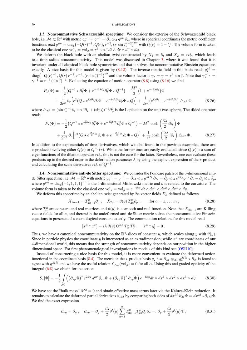
70 8. APPLICATIONS

1.3. Noncommutative Schwarzschild spacetime: We consider the exterior of the Schwarzschild blackhole, i.e.M⊂ R4 with metric g−1

? = g−1 = ∂µ⊗A gµν ∂ν , where in spherical coordinates the metric coefficientfunctions read gµν = diag

(−Q(r)−1, Q(r), r−2, (r sin ζ)−2

)µνwith Q(r) = 1− rs

r . The volume form is takento be the classical one vol? = volg = r2 sin ζ dt ∧ dr ∧ dζ ∧ dφ.

We deform the black hole with an abelian twist constructed by X1 = ∂t and X2 = r∂r, which leadsto a time-radius noncommutativity. This model was discussed in Chapter 3, where it was found that it isinvariant under all classical black hole symmetries and that it solves the noncommutative Einstein equationsexactly. A nice basis for this model is given by (8.12). The inverse metric field in this basis reads gab? =

diag(−Q(r)−1, Q(r) r−2, r−2, (r sin ζ)−2

)aband the volume factor is γ? = γ = r3 sin ζ. Note that γ−1?

? =

γ−1 = r−3 (sin ζ)−1. Evaluating the equation of motion operator (8.8) using (8.16) we find

P?(Φ) = −1

2

(Q−1 ? ∂2

t Φ + e−i3λ∂t∂2t Φ ? Q−1

)− M2

2

(1 + e−i3λ∂t

)Φ

+1

2r2∂r

[r2(Q ? eiλ∂t∂rΦ + e−i4λ∂t∂rΦ ? Q

)]+

1

2r2

(eiλ∂t + e−i4λ∂t

)4S2 Φ , (8.26)

where4S2 = (sin ζ)−1∂ζ sin ζ∂ζ + (sin ζ)−2∂2φ is the Laplacian on the unit two-sphere. The tilded operator

reads

P?(Φ) = −1

2

(Q−1 ? e

i3λ2 ∂t∂2

t Φ + e−i3λ2 ∂t∂2

t Φ ? Q−1)−M2 cosh

(3λ

2i∂t

)Φ

+1

2r2∂r

[r2(Q ? e

i5λ2 ∂t∂rΦ + e−

i5λ2 ∂t∂rΦ ? Q

)]+

1

r2cosh

(5λ

2i∂t

)4S2 Φ . (8.27)

In addition to the exponentials of time derivatives, which we also found in the previous examples, there are?-products involving either Q(r) or Q−1(r). While the former ones are easily evaluated, since Q(r) is a sum ofeigenfunctions of the dilation operator r∂r, this is not the case for the latter. Nevertheless, one can evaluate theseproducts up to the desired order in the deformation parameter λ by using the explicit expression of the ?-productand calculating the scale derivatives r∂r of Q−1.

1.4. Noncommutative anti-de Sitter spacetime: We consider the Poincare patch of the 5-dimensional anti-de Sitter spacetime, i.e.M = R5 with metric g−1

? = g−1 = ∂M ⊗A gMN ∂N = ∂µ⊗A e2kygµν ∂ν + ∂y ⊗A ∂y ,where gµν = diag

(−1, 1, 1, 1

)µνis the 4-dimensional Minkowski metric and k is related to the curvature. The

volume form is taken to be the classical one vol? = volg = e−4ky dt ∧ dx1 ∧ dx2 ∧ dx3 ∧ dy.We deform this spacetime by an abelian twist generated by 2n vector fields Xα defined as follows

X2a−1 = Tµ2a−1∂µ , X2a = ϑ(y)Tµ2a∂µ , for a = 1, . . . , n , (8.28)

where Tµα are constant and real matrices and ϑ(y) is a smooth and real function. Note that X2a−1 are Killingvector fields for all a, and therewith the undeformed anti-de Sitter metric solves the noncommutative Einsteinequations in presence of a cosmological constant exactly. The commutation relations for this model read

[xµ ?, xν ] = iλ ϑ(y) Θαβ Tµα Tνβ , [xµ ?, y] = 0 . (8.29)

Thus, we have a canonical noncommutativity on the R4-slices of constant y, which scales along y with ϑ(y).Since in particle physics the coordinate y is interpreted as an extradimension, while xµ are coordinates of our4-dimensional world, this means that the strength of noncommutativity depends on our position in the higherdimensional space. For first phenomenological investigations in models of this kind see [OSU10].

Instead of constructing a nice basis for this model, it is more convenient to evaluate the deformed actionfunctional in the coordinate basis (8.4). The metric in the ?-product basis g−1

? = ∂M ⊗A? gMN? ? ∂N is found to

agree with gMN and we have the useful relation LXα(volg) = 0 for all α. Using this and graded cyclicity of theintegral (6.8) we obtain for the action

S?[Φ] = −1

2

∫M

((∂?µΦ

)∗e2ky gµν ∂?νΦ +

(∂?yΦ

)∗∂?yΦ

)e−4kydt ∧ dx1 ∧ dx2 ∧ dx3 ∧ dy . (8.30)

We have set the “bulk mass” M2 = 0 and obtain effective mass terms later via the Kaluza-Klein reduction. Itremains to calculate the deformed partial derivatives ∂?M by comparing both sides of dxM ∂MΦ = dxM ?∂?MΦ.We find the exact expression

∂?µ = ∂µ , ∂?y = ∂y +iλ

2ϑ′(y)

n∑a=1

Tµ2a−1Tν2a∂µ∂ν =: ∂y +

iλ

2ϑ′(y)T , (8.31)

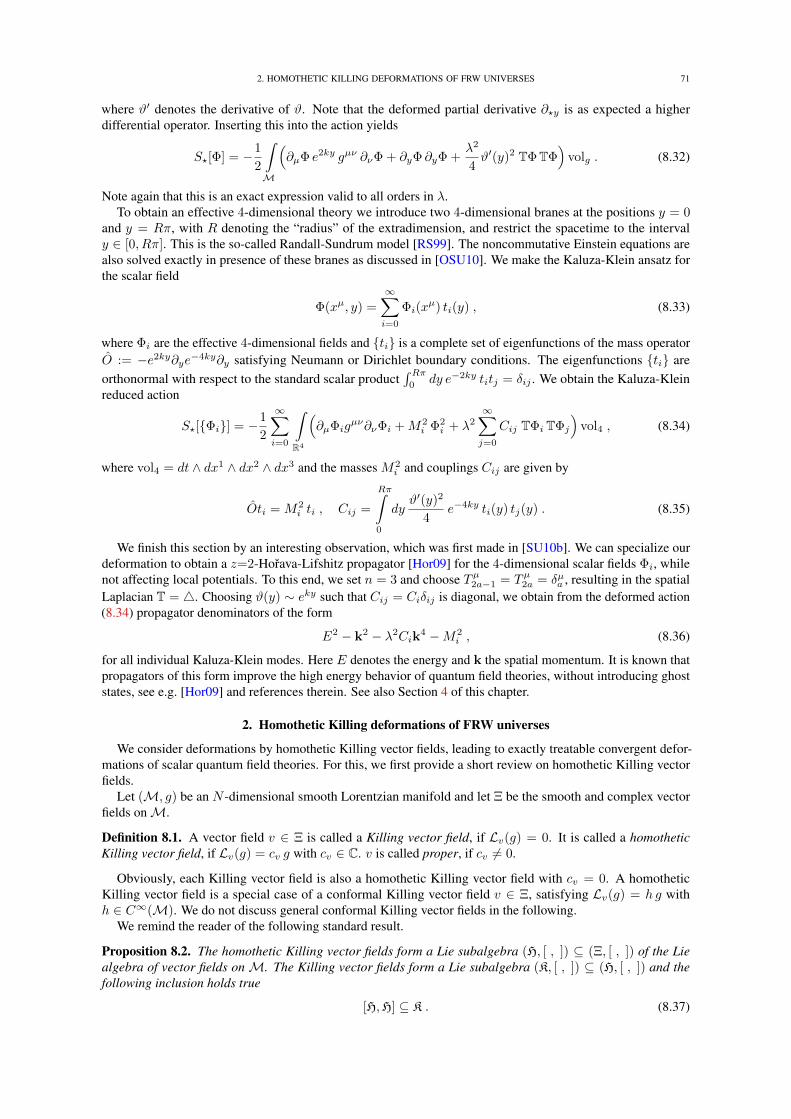
2. HOMOTHETIC KILLING DEFORMATIONS OF FRW UNIVERSES 71

where ϑ′ denotes the derivative of ϑ. Note that the deformed partial derivative ∂?y is as expected a higherdifferential operator. Inserting this into the action yields

S?[Φ] = −1

2

∫M

(∂µΦ e2ky gµν ∂νΦ + ∂yΦ ∂yΦ +

λ2

4ϑ′(y)2 TΦTΦ

)volg . (8.32)

Note again that this is an exact expression valid to all orders in λ.To obtain an effective 4-dimensional theory we introduce two 4-dimensional branes at the positions y = 0

and y = Rπ, with R denoting the “radius” of the extradimension, and restrict the spacetime to the intervaly ∈ [0, Rπ]. This is the so-called Randall-Sundrum model [RS99]. The noncommutative Einstein equations arealso solved exactly in presence of these branes as discussed in [OSU10]. We make the Kaluza-Klein ansatz forthe scalar field

Φ(xµ, y) =

∞∑i=0

Φi(xµ) ti(y) , (8.33)

where Φi are the effective 4-dimensional fields and ti is a complete set of eigenfunctions of the mass operatorO := −e2ky∂ye

−4ky∂y satisfying Neumann or Dirichlet boundary conditions. The eigenfunctions ti areorthonormal with respect to the standard scalar product

∫ Rπ0

dy e−2ky titj = δij . We obtain the Kaluza-Kleinreduced action

S?[Φi] = −1

2

∞∑i=0

∫R4

(∂µΦig

µν∂νΦi +M2i Φ2

i + λ2∞∑j=0

Cij TΦi TΦj

)vol4 , (8.34)

where vol4 = dt ∧ dx1 ∧ dx2 ∧ dx3 and the masses M2i and couplings Cij are given by

Oti = M2i ti , Cij =

Rπ∫0

dyϑ′(y)2

4e−4ky ti(y) tj(y) . (8.35)

We finish this section by an interesting observation, which was first made in [SU10b]. We can specialize ourdeformation to obtain a z=2-Horava-Lifshitz propagator [Hor09] for the 4-dimensional scalar fields Φi, whilenot affecting local potentials. To this end, we set n = 3 and choose Tµ2a−1 = Tµ2a = δµa , resulting in the spatialLaplacian T = 4. Choosing ϑ(y) ∼ eky such that Cij = Ciδij is diagonal, we obtain from the deformed action(8.34) propagator denominators of the form

E2 − k2 − λ2Cik4 −M2

i , (8.36)

for all individual Kaluza-Klein modes. Here E denotes the energy and k the spatial momentum. It is known thatpropagators of this form improve the high energy behavior of quantum field theories, without introducing ghoststates, see e.g. [Hor09] and references therein. See also Section 4 of this chapter.

2. Homothetic Killing deformations of FRW universes

We consider deformations by homothetic Killing vector fields, leading to exactly treatable convergent defor-mations of scalar quantum field theories. For this, we first provide a short review on homothetic Killing vectorfields.

Let (M, g) be an N -dimensional smooth Lorentzian manifold and let Ξ be the smooth and complex vectorfields onM.

Definition 8.1. A vector field v ∈ Ξ is called a Killing vector field, if Lv(g) = 0. It is called a homotheticKilling vector field, if Lv(g) = cv g with cv ∈ C. v is called proper, if cv 6= 0.

Obviously, each Killing vector field is also a homothetic Killing vector field with cv = 0. A homotheticKilling vector field is a special case of a conformal Killing vector field v ∈ Ξ, satisfying Lv(g) = h g withh ∈ C∞(M). We do not discuss general conformal Killing vector fields in the following.

We remind the reader of the following standard result.

Proposition 8.2. The homothetic Killing vector fields form a Lie subalgebra (H, [ , ]) ⊆ (Ξ, [ , ]) of the Liealgebra of vector fields onM. The Killing vector fields form a Lie subalgebra (K, [ , ]) ⊆ (H, [ , ]) and thefollowing inclusion holds true

[H,H] ⊆ K . (8.37)

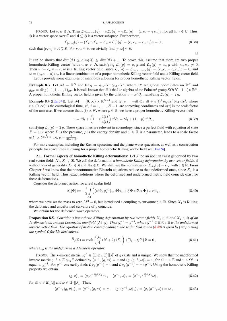
72 8. APPLICATIONS

PROOF. Let v, w ∈ H. Then Lβ v+γ w(g) = βLv(g) + γLw(g) = (β cv + γ cw)g, for all β, γ ∈ C. Thus,H is a vector space over C and K ⊆ H is a vector subspace. Furthermore,

L[v,w](g) = (Lv Lw − Lw Lv)(g) = (cv cw − cw cv)g = 0 , (8.38)

such that [v, w] ∈ K ⊆ H. For v, w ∈ K we trivially find [v, w] ∈ K.

It can be shown that dim(K) ≤ dim(H) ≤ dim(K) + 1. To prove this, assume that there are two properhomothetic Killing vector fields v, w ∈ H, satisfying Lv(g) = cv g and Lw(g) = cw g with cv, cw 6= 0.Then u := cw v − cv w is a Killing vector field, since Lu(g) = Lcw v−cv w(g) = (cwcv − cvcw)g = 0, andw = (cw v − u)/cv is a linear combination of a proper homothetic Killing vector field and a Killing vector field.

Let us provide some examples of manifolds allowing for proper homothetic Killing vector fields.

Example 8.3. Let M = RN and let g = gµνdxµ ⊗A dxν , where xµ are global coordinates on RN and

gµν = diag(−1, 1, . . . , 1)µν . It is well-known that K is the Lie algebra of the Poincare group SO(N−1, 1)nRN .A proper homothetic Killing vector field is given by the dilation v = xµ∂µ, satisfying Lv(g) = 2 g.

Example 8.4 ([Ear74]). Let M = (0,∞) × RN−1 and let g = −dt ⊗A dt + a(t)2 δijdxi ⊗A dxj , where

t ∈ (0,∞) is the cosmological time, xi, i = 1, . . . , N − 1, are comoving coordinates and a(t) is the scale factorof the universe. If we assume that a(t) ∝ tp, where p ∈ R, we have a proper homothetic Killing vector field

v = t∂t +

(1− t a(t)

a(t)

)xi∂i = t∂t + (1− p)xi∂i , (8.39)

satisfying Lv(g) = 2 g. These spacetimes are relevant in cosmology, since a perfect fluid with equation of stateP = ωρ, where P is the pressure, ρ is the energy density and ω ∈ R is a parameter, leads to a scale factora(t) ∝ t

23(ω+1) , i.e. p = 2

3(ω+1) .

For more examples, including the Kasner spacetime and the plane-wave spacetime, as well as a constructionprinciple for spacetimes allowing for a proper homothetic Killing vector field see [Ear74].

2.1. Formal aspects of homothetic Killing deformations: Let F be an abelian twist generated by tworeal vector fields X1, X2 ∈ Ξ. We call the deformation a homothetic Killing deformation by two vector fields, ifwithout loss of generality X1 ∈ K and X2 ∈ H. We shall use the normalization LX2

(g) = c g, with c ∈ R. FromChapter 3 we know that the noncommutative Einstein equations reduce to the undeformed ones, since X1 is aKilling vector field. Thus, exact solutions where the deformed and undeformed metric field coincide exist forthese deformations.

Consider the deformed action for a real scalar field

S?[Φ] := −1

2

∫M

(〈〈dΦ, g−1

? 〉?,dΦ〉? + ξΦ ?R ? Φ)? volg , (8.40)

where we have set the mass to zero M2 = 0, but introduced a coupling to curvature ξ ∈ R. Since X1 is Killing,the deformed and undeformed curvature of g coincide.

We obtain for the deformed wave operators

Proposition 8.5. Consider a homothetic Killing deformation by two vector fields X1 ∈ K and X2 ∈ H of anN -dimensional smooth Lorentzian manifold (M, g). Then g−1

? = g−1, where g−1 ∈ Ξ⊗A Ξ is the undeformedinverse metric field. The equation of motion corresponding to the scalar field action (8.40) is given by (suppressingthe symbol L for Lie derivatives)

P?(Φ) = cosh

(λc

4(N + 2) iX1

) (g − ξR

)Φ = 0 , (8.41)

where g is the undeformed d’Alembert operator.

PROOF. The ?-inverse metric g−1? ∈

(Ξ⊗A Ξ

)[[λ]] of g exists and is unique. We show that the undeformed

inverse metric g−1 ∈ Ξ⊗A Ξ defined by 〈g−1, 〈g, v〉〉 = v and 〈g, 〈g−1, ω〉〉 = ω, for all v ∈ Ξ and ω ∈ Ω1, isequal to g−1

? . For g−1 one easily finds LX1(g−1) = 0 and LX2

(g−1) = −c g−1. Using the homothetic Killingproperty we obtain

〈g, v〉? = 〈g, e− iλc2 X1v〉 , 〈g−1, ω〉? = 〈g−1, eiλc2 X1ω〉 , (8.42)

for all v ∈ Ξ[[λ]] and ω ∈ Ω1[[λ]]. Thus,

〈g−1, 〈g, v〉?〉? = 〈g−1, 〈g, v〉〉 = v , 〈g, 〈g−1, ω〉?〉? = 〈g, 〈g−1, ω〉〉 = ω , (8.43)

2. HOMOTHETIC KILLING DEFORMATIONS OF FRW UNIVERSES 73

by using the invariance of g and g−1 under X1.For the metric volume form one finds that LX1

(volg) = 0 and LX2(volg) = cN

2 volg . For the curvature we haveLX1(R) = 0 and LX2(R) = −cR [AC10]. Using this, (8.42) and graded cyclicity in order to remove one ?under the integral, we obtain for the variation of the action (8.40) by functions δΦ of compact support

δS?[Φ] =

∫M

δΦ volg cosh

(λc

4(N + 2)iX1

) (g − ξR

)Φ . (8.44)

Remark 8.6. Note that in case we deform by two Killing vector fields X1, X2 ∈ K we have c = 0 and theequation of motion operator P? (8.41) is undeformed. This is a generalization of the well-known result that thedynamics of a free scalar field theory on the Moyal-Weyl deformed Minkowski spacetime is undeformed.

Let now (M, g) be a connected, time-oriented and globally hyperbolic Lorentzian manifold. The constructionof the Green’s operators corresponding to the deformed equation of motion operator (8.41) is straightforward.We define

∆?± := ∆± cosh

(λc

4(N + 2) iX1

)−1

, (8.45)

where the inverse of cosh(λc4 (N + 2) iX1

)is understood in terms of formal power series and ∆± are the

unique retarded and advanced Green’s operators corresponding to the undeformed equation of motion operatorP = g − ξR. We find

P? ∆?± = idC∞0 (M)[[λ]] , (8.46a)

∆?± P?|C∞0 (M)[[λ]] = idC∞0 (M)[[λ]] , (8.46b)

and the support property

supp(∆?±(ϕ)

)⊆ J±

(supp(ϕ)

), (8.46c)

for all ϕ ∈ C∞0 (M), since the noncommutative corrections to ∆± are finite order differential operators at everyorder in λ.

The retarded-advanced Green’s operator for this model is

∆? := ∆?+ − ∆?− = ∆ cosh

(λc

4(N + 2) iX1

)−1

, (8.47)

resulting in the following symplectic structure on V? = C∞0 (M,R)[[λ]]/P?[C∞0 (M,R)[[λ]]]

ω?([ϕ], [ψ]) =(ϕ, ∆?(ψ)

). (8.48)

The symplectic isomorphism to the undeformed symplectic R[[λ]]-module (V [[λ]], ω) is obviously given by

S : V? → V [[λ]] , [ϕ] 7→ [Sϕ] , (8.49)

where

S =

√cosh

(λc

4(N + 2) iX1

)−1

. (8.50)

We have ω?([ϕ], [ψ]) = ω(S[ϕ],S[ψ]), for all [ϕ], [ψ] ∈ V?.

Remark 8.7. Note that the retarded and advanced symplectic isomorphism S± of Chapter 7 coincide forhomothetic Killing deformations by two vector fields.

The quantum field theory can be constructed along the lines of Chapter 6.This shows that the formal theory of homothetic Killing deformations by two vector fields is very simple. This

allows us to discuss convergent examples, which is the main goal of the remaining part of this section.

2.2. A spatially flat FRW toy-model: We apply the formalism presented in the previous subsectionto a toy-model. We use a special choice of the FRW spacetime of Example 8.4. Let M = (0,∞) × R3,i.e. N = 4, and let t and xi, i ∈ 1, 2, 3, be global coordinates. The metric field we consider is given byg = −dt⊗A dt+ t2 δijdx

i ⊗A dxj . Note that in our conventions the spatial coordinates xi are dimensionless.The reason for choosing the scale factor a(t) ∝ t is that in this case a proper homothetic Killing vector field isgiven by X2 = t∂t and all Killing vector fields commute with X2. The most general real Killing vector field isk(ξ,η) := ξi∂i + ηkεkijx

i∂j , where ξ, η ∈ R3.

74 8. APPLICATIONS

The undeformed theory: We start by collecting useful formulae of the undeformed free, real, massless andcurvature coupled scalar quantum field theory on our particular FRW spacetime. They will be used later to studythe noncommutative deformation. We frequently use the Fourier transformation on the spatial hypersurfaces R3

defined by t = const. We indicate this transformation by a hat and use the conventions

ϕ(t, k) =

∫R3

d3x eikx ϕ(t, x) , ϕ(t, x) =

∫R3

d3k

(2π)3e−ikx ϕ(t, k) . (8.51)

The wave operator P = g − ξR in Fourier space is given by

P(ϕ)(t, k) = −

(∂2t +

3

t∂t +

k2 + 6ξ

t2

)ϕ(t, k) . (8.52)

The corresponding retarded and advanced Green’s operators read

∆±(ϕ)(t, k) = −

t∫t±

dττ3 ∆(t, τ, k) ϕ(τ, k) , (8.53)

where t+ = 0, t− =∞ and

∆(t, τ, k) =t√

1−k2−6ξτ−√

1−k2−6ξ − t−√

1−k2−6ξτ√

1−k2−6ξ

2tτ√

1− k2 − 6ξ. (8.54)

We obtain for the retarded-advanced Green’s operator ∆ = ∆+ −∆−

∆(ϕ)(t, k) = −

∞∫0

dττ3 ∆(t, τ, k) ϕ(τ, k) , (8.55)

resulting in the pre-symplectic structure

ω(ϕ,ψ) = −∞∫

0

dtt3∞∫

0

dττ3

∫R3

d3k

(2π)3ϕ(t,−k) ∆(t, τ, k) ψ(τ, k) . (8.56)

We define the geometric action of (R, a) ∈ SO(3) nR3 on C∞(M) by(α(R,a)ϕ

)(t, x) := ϕ

(t, R−1(x− a)

). (8.57)

In Fourier space, these transformations are given by(α(R,a)ϕ

)(t, k) = eika ϕ(t, R−1k) . (8.58)

We easily obtain that SO(3) n R3 ⊆ G(V,ω) are symplectic automorphisms of the symplectic vector space(V, ω) =

(C∞0 (M,R)/P [C∞0 (M,R)], ω

).

In this section we are working in a convergent framework and all symplectic modules are vector spaces overR. Thus, we can apply the powerful theory of CCR-algebras in order to quantize the symplectic vector space(V, ω), i.e. in order to define the quantum field theory, see Chapter 5.

The deformed theory with X1 = ∂1: We study a convergent deformation of our FRW model. We chooseX1 = ∂1, i.e. a translation along the x1-direction. The flow generated by X1 = ∂1 is noncompact. The condition[X1, X2] = 0, which is required for our deformations, is satisfied. Our strategy is to make a convergent definitionof the maps S =

√cosh(3λi∂1)−1 and S−1 =

√cosh(3λi∂1), which enter the construction of the deformed

quantum field theory. Using these maps we construct the deformed quantum field theory and investigate itsproperties.

We first define a convenient space of functions C∞0,S (M) ⊂ C∞(M), whereM = (0,∞)× R3. A functionϕ ∈ C∞(M) is in C∞0,S (M), if (1.) for all fixed x ∈ R3 ϕ(t, x) ∈ C∞0 ((0,∞)) and (2.) for all fixed t ∈ (0,∞)

ϕ(t, x) ∈ S (R3) is a Schwartz function. We have C∞0 (M) ⊂ C∞0,S (M) ⊂ C∞(M). The spatial Fouriertransformation is an automorphism of C∞0,S (M), i.e. let ϕ(t, x) ∈ C∞0,S (M) then ϕ(t, k) ∈ C∞0,S (M) and viceversa.

Using the spatial Fourier transformation we define the map S : C∞0,S (M)→ C∞0,S (M) by(Sϕ)(t, k) :=

√cosh(3λk1)−1 ϕ(t, k) . (8.59)

This map is injective. The inverse map S−1 : S[C∞0,S (M)

]→ C∞0,S (M) is given by(

S−1ϕ)(t, k) =

√cosh(3λk1) ϕ(t, k) . (8.60)

2. HOMOTHETIC KILLING DEFORMATIONS OF FRW UNIVERSES 75

Note that S[C∞0,S (M)

]⊂ C∞0,S (M), since S

[C∞0,S (M)

]includes only functions with Fourier spectra decreas-

ing faster than e−3λ|k1|/2 for large |k1|.We can now construct the deformed quantum field theory. For simplifying the notation we drop the tilde on

the deformed maps. We define the deformed Green’s operators by

∆?±(ϕ)(t, k) := ∆±

(S2ϕ

)(t, k) = −

t∫t±

dττ3 ∆(t, τ, k)

cosh(3λk1)ϕ(τ, k) . (8.61)

This results in the deformed retarded-advanced Green’s operator

∆?

(ϕ)(t, k) = −

∞∫0

dττ3 ∆(t, τ, k)

cosh(3λk1)ϕ(τ, k) , (8.62)

and the deformed pre-symplectic structure on C∞0 (M,R)

ω?(ϕ,ψ) = −∞∫

0

dtt3∞∫

0

dττ3

∫R3

d3k

(2π)3ϕ(t,−k)

∆(t, τ, k)

cosh(3λk1)ψ(τ, k) . (8.63)

The deformed retarded-advanced Green’s operator satisfies Ker(∆?) = Ker(∆). To prove this, let ϕ ∈C∞0 (M,R). Using (8.62) we find

∆?

(ϕ)(t, k) = cosh(3λk1)−1 ∆

(ϕ)(t, k) , (8.64)

and the proof follows from the positivity of cosh(3λk1)−1. From the general considerations in Chapter 5we know that Ker(∆) = P [C∞0 (M,R)]. Thus, we can define the deformed symplectic vector space as(V?, ω?) :=

(C∞0 (M,R)/P [C∞0 (M,R)], ω?

). Different to formal deformation quantization this is now a vector

space over R and not a module over the ring R[[λ]].The construction of the deformed quantum field theory in terms of a CCR-representation of (V?, ω?) can be

performed analogously to the undeformed case (see Chapter 5), since (V?, ω?) is symplectic vector space over R.This results in a unique (up to ∗-isomorphisms) deformed CCR-algebra A? describing the deformed quantumfield theory.

Physical features of the deformed theory: Let us investigate some physical features of the deformed fieldtheory. In the following we assume that λ > 0. We study in more detail the map S2 acting on C∞0 (M). Notethat in position space this map is given by the following convolution(

S2ϕ)(t, x) =

∫R

dy1 1

6λ cosh(π(x1 − y1)/6λ

) ϕ(t, y1, x2, x3) , (8.65)

for all ϕ ∈ C∞0 (M). It is easy to check that the image S2[C∞0 (M)] 6⊆ C∞0 (M). For this assume thatϕ ∈ C∞0 (M) is a positive semidefinite function localized in some compact region K ⊂M, e.g. a bump function.Since the convolution kernel is of noncompact support and strictly positive, the resulting function S2ϕ is ofnoncompact support in the x1-direction. However, S2ϕ will be of rapid decrease, since the convolution kernel isa Schwartz function.

Physically, this means that causality is lost. We immediately obtain that the relation ∆?±(ϕ) ⊆ J±(supp(ϕ)

),

for all ϕ ∈ C∞0 (M), is violated. Thus, external sources couple in a nonlocal way to our deformed field theory,which is a feature not present in the commutative counterpart. Since ∆?± depends on the value of λ through(8.65), we can determine λ (in principle) by measuring the response of the field to external excitations.

Consider now the deformed pre-symplectic structure in position space

ω?(ϕ,ψ) =

∫M

ϕ∆(S2ψ) volg . (8.66)

Due to the appearance of the nonlocal map S2 (8.65) there are functions ϕ,ψ with causally disconnected supportsatisfying ω?(ϕ,ψ) 6= 0. For our choice of deformation (X1 = ∂1 and X2 = t∂t) this nonlocality only affectsthe x1-direction, but its range is infinite. We still obtain that ω?(ϕ,ψ) = 0 if arbitrary translations of supp(ψ)along the x1-direction and supp(ϕ) are causally disconnected. In the quantum field theory described by A? thisnonlocal behavior leads to a noncommutativity between observables located in spacelike separated regions inspacetime.

76 8. APPLICATIONS

∗-isomorphism between the deformed and a nonstandard undeformed quantum field theory: Wehave shown in the previous paragraph that S2[C∞0 (M,R)] 6⊆ C∞0 (M,R). The map S defined in (8.59) canalso be written in terms of a convolution in position space, similar to S2, but the convolution kernel is morecomplicated. Its explicit form is not of importance to us.

From S2[C∞0 (M,R)] 6⊆ C∞0 (M,R) we can infer that S[C∞0 (M,R)] 6⊆ C∞0 (M,R). To prove this, assumethat S[C∞0 (M,R)] ⊆ C∞0 (M,R) then we would find S2[C∞0 (M,R)] ⊆ C∞0 (M,R) by applying S twice,which contradicts the observation above.

The bijective map S : C∞0 (M,R) → C∞img(M,R) ⊂ C∞0,S (M,R) induces a symplectic isomorphismbetween (V?, ω?) and (Vimg, ω) :=

(C∞img(M,R)/S

[P [C∞0 (M,R)]

], ω), i.e. the deformed field theory can be

related to a nonstandard undeformed one. Using Corollary 5.13, this map induces a unique ∗-isomorphismbetween the CCR-algebras A? and Aimg.

Let us consider the symmetries of the deformed quantum field theory. As we have seen above, the undeformedsymplectic vector space (V, ω) contains SO(3) nR3 in the group of symplectic automorphisms. The represen-tation is given by the geometric action (8.58). However, the space C∞img(M,R) ⊂ C∞0,S (M,R), which servesas a pre-symplectic vector space for (Vimg, ω), is not invariant under the action of SO(3) nR3. The preservedsubgroup is SO(2) nR3, where the SO(2)-rotation preserves the x1-axis. Thus, the deformed quantum fieldtheory A? is ∗-isomorphic to a nonsymmetric undeformed quantum field theory Aimg. This, in particular, showsthat the results of Chapter 7 are restricted to formal deformation quantization.

Physical interpretation: As shown above, we do not have a ∗-isomorphism between the deformed quantumfield theory A? and the standard undeformed quantum field theory A for convergent deformations. This fact hasa very natural physical interpretation, which we will explain now.

Consider the extended symplectic vector space (Vext, ω) :=(C∞0,S (M,R)/Ker(∆), ω

). This vector space

carries a representation of SO(3) nR3 via the geometric action (8.58). A CCR-representation of (Vext, ω) yieldsthe extended CCR-algebra Aext. Aext carries a representation of the group SO(3) nR3. The algebra Aext is anextension of the usual CCR-algebra A, where also certain delocalized observables are allowed. This alreadyshows that Aext is more suitable to study the connection between deformed and undeformed quantum fieldtheories.

Analogously to above, we define the deformed extended symplectic vector space (Vext?, ω?) := (Vext, ω?) anda CCR-representation of (Vext?, ω?) yields the deformed extended CCR-algebra Aext?.

The bijective map S : C∞0,S (M,R) → C∞img′(M,R) ⊂ C∞0,S (M,R) induces a symplectic isomorphismbetween (Vext?, ω?) and (Vimg′ , ω). Furthermore, S induces a symplectic embedding (Vext?, ω?) → (Vext, ω).Using Corollary 5.13 we can induce a unique ∗-isomorphism between the CCR-algebras Aext? and Aimg′ , as wellas a unique injective, but not surjective, ∗-homomorphism fromAext? toAext. We thus haveAext? ' Aimg′ ⊂ Aext.

Physically, this means that due to the noncommutative deformation the quantum field theory looses observables.Since C∞img′(M,R) depends on the value of λ, the observables we loose also depend on the value of λ. Note thatall functions in C∞img′(M,R) have Fourier spectra which decrease faster than e−3λ|k1|/2 for large |k1|. Increasingλ leads to a sharper localization in momentum space and therefore a weaker localization in position space. Thus,the deformed quantum field theory looses those observables that are strongly localized in position space, whichis physically very natural.

Induction of states: The injective ∗-homomorphism S : A? → Aext, or its extension Sext : Aext? → Aext,is useful for inducing states via the pull-back. Assume that we have an SO(3)nR3-invariant state Ωext : Aext → C.Defining Ω? := Ωext S : A? → C induces a state on A?, which is invariant under the unbroken symmetrygroup SO(2) nR3. The same holds true for Ωext? := Ωext Sext : Aext? → C.

Noncommutative effects on the cosmological power spectrum: In order to show that our models lead tonontrivial physical effects we briefly discuss the cosmological power spectrum. We shall work with the extendedCCR-algebras Aext? and Aext. Let Ω : Aext → C be a regular, quasi-free and translation invariant (i.e. R3-invariant) state. We denote by

(H, π, |0〉

)the GNS-representation of (Aext,Ω). Employing the ∗-homomorphism

Sext : Aext? → Aext we obtain a representation π? = π Sext of Aext? onH. The vector |0〉 might not be cyclicwith respect to this representation and we define the Hilbert subspaceH? = π?[Aext?]|0〉. By the GNS-Theoremthe cyclic representation

(H?, π?, |0〉

)is unitary equivalent to the GNS-representation of (Aext?,Ω?).

Using regularity of the state Ω we can define the selfadjoint linear field operators Φ(v) ∈ L(D), v ∈ Vext, asthe generators of the Weyl operators π

(W (v)

)∈ B(H). They are related to the deformed field operators Φ?

by Φ?(v) = Φ(Sv) ∈ L(D), which are the generators of π?(W?(v)

)= π

(W (Sv)

). Thus, n-point functions of

the deformed field operators can be related to n-point functions of the undeformed ones. Due to the quasi-freeassumption on the state Ω only the 2-point function is of interest and all higher n-point functions can be derived

2. HOMOTHETIC KILLING DEFORMATIONS OF FRW UNIVERSES 77

from it, in the undeformed and also deformed case. We define the deformed 2-point function

Ω?2(ϕ,ψ) := 〈0|Φ?([ϕ])Φ?([ψ])|0〉 = 〈0|Φ([Sϕ])Φ([Sψ])|0〉 = Ω2(Sϕ, Sψ) , (8.67)

for all ϕ,ψ ∈ C∞0 (M,R), where Ω2 is the undeformed 2-point function.In order to calculate the power spectrum we require the kernel of Ω2 (Ω?2) in Fourier space. Making use of

the translation invariance of the state Ω we have

Ω2(ϕ,ψ) =

∞∫0

dtt3∞∫

0

dττ3

∫R3

d3k

(2π)3Ω2(t, τ, k) ϕ(t, k) ψ(τ,−k) . (8.68)

It follows that

Ω?2(ϕ,ψ) = Ω2(Sϕ, Sψ) =

∞∫0

dtt3∞∫

0

dττ3

∫R3

d3k

(2π)3

Ω2(t, τ, k)

cosh(3λk1)ϕ(t, k) ψ(τ,−k) . (8.69)

The undeformed power spectrum is then given by

P(t, k) := Ω2(t, t, k) , (8.70)

and the deformed power spectrum reads

P?(t, k) =P(t, k)

cosh(3λk1). (8.71)

The physical feature of P? compared to P is an exponential loss of power for large |k1|.

2.3. A spatially compact FRW toy-model: The flow generated by the vector field X1 = ∂1 in the modelabove is noncompact. We now investigate if deformations along vector fields X1 generating compact flowsdiffer from the noncompact case. A possible choice of toy-model would be the model of Subsection 2.2 withX1 = x2∂3 − x3∂2, i.e. a rotation around the x1-axis, and X2 = t∂t.

However, there is an even simpler model which we can use for our studies. Consider the manifoldM =(0,∞) × S1, where S1 is the 1-dimensional circle, equipped with the metric g = −dt ⊗A dt + t2dφ ⊗A dφ.Here t ∈ (0,∞) denotes time and φ ∈ [0, 2π) is the angle. A proper homothetic Killing vector field is X2 = t∂tand X1 = 2∂φ is a Killing vector field.1 The necessary condition [X1, X2] = 0 is satisfied. The calculation ofthe undeformed wave operator P = g − ξR and the corresponding retarded and advanced Green’s operators∆± is standard. We do not need to present the explicit results here.

We investigate in detail the convergent version of S =√

cosh(3λi∂φ)−1 and S−1 =√

cosh(3λi∂φ). For thiswe make use of the Fourier transformation on the spatial hypersurfaces S1. Since S1 is compact, the momentan ∈ Z are discrete. We define in Fourier space(

Sϕ)(t, n) :=

√cosh(3λn)−1 ϕ(t, n) , (8.72a)(

S−1ϕ)(t, n) =

√cosh(3λn) ϕ(t, n) . (8.72b)

It remains to discuss the domains of the maps S and S−1. Note that a function ϕ on the circle S1 is smooth ifand only if its Fourier spectrum is of rapid decrease. From this and (8.72a) we infer S : C∞0 (M)→ C∞0 (M).However, S−1 can not be defined on all of C∞0 (M), provided we restrict the image of S−1 to smooth functions.Since S is injective, we find the isomorphism S : C∞0 (M)→ C∞img(M) ⊂ C∞0 (M).

Analogously to the situation where X1 generates a noncompact flow we find that the symplectic isomorphismmaps between the deformed symplectic vector space (V?, ω?) and a nonstandard undeformed symplectic vectorspace (Vimg, ω). In case of models with additional isometries (Vimg, ω) carries only a representation of theunbroken subgroup. Furthermore, the map S embeds (V?, ω?) into the undeformed symplectic vector space(V, ω). This is also analogous to the situation before, with the difference that we do not have to extend thesymplectic vector space. All linear symplectic maps induce unique injective ∗-homomorphisms between thecorresponding CCR-algebras due to Corollary 5.13.

We find again that the deformed quantum field theory looses observables, depending on the value of λ. Sincethe functions in C∞img(M) have Fourier spectra which decrease faster than e−3λ|n|/2 for large |n| we loose thoseobservables that are strongly localized in position space.

1 The factor 2 in the definition of X1 is a convenient normalization.

78 8. APPLICATIONS

2.4. Physical inequivalence of the deformed and undeformed quantum field theory: In this subsectionwe collect arguments that our deformed quantum field theory is physically inequivalent to standard commutativequantum field theories. This discussion is very important, since it has been shown [Poh68, BP68] that it isnot possible in the framework of Wightman quantum field theory on the undeformed Minkowski spacetime toconstruct a nonlocal theory with nonlocalities in the commutator function that fall off faster than exponentially.Indeed, Wightman theories with a faster than exponentially vanishing nonlocality in the commutator function oftwo fundamental fields are equivalent to local quantum field theories. Therefore, we have to ensure that a similarresult does not apply to our deformed models.

The first sign for an inequivalence of our deformed quantum field theories to standard commutative ones comesfrom the nonlocal behavior of the deformed Green’s operators ∆?± discussed above. Coupling our deformedtheories to external sources (or introducing perturbative interactions) then leads to nonlocal effects which inprinciple can be used to measure the deformation parameter λ.

The second sign comes from the form of the deformed power spectrum (8.71). Commutative quantum fieldtheories on FRW spacetimes typically have a power spectrum, which goes as P(t, k) ∝ |k|ns−4, where nsis the spectral index. Our deformed power spectrum (8.71) shows, additionally to this power-law behavior,an exponential drop-off for large |k1|. Such a drop-off, and with this also the value of λ, can in principle bemeasured.

The third sign comes from the nonlocality of the symplectic structure (8.66). We consider analogously to[Poh68, BP68] the correlation function

〈0|[Φ?([ϕ1]),Φ?([ϕ2])

]Φ?([ϕ3])Φ?([ϕ4])|0〉 , (8.73)

which, in our case, reduces due to the canonical commutation relations to

〈0|[Φ?([ϕ1]),Φ?([ϕ2])

]Φ?([ϕ3])Φ?([ϕ4])|0〉 = i ω?(ϕ1, ϕ2) 〈0|Φ?([ϕ3])Φ?([ϕ4])|0〉

= i ω?(ϕ1, ϕ2) Ω?2(ϕ3, ϕ4) . (8.74)

Since, as explained above, the commutator function ω? can be nonzero for functions ϕ1, ϕ2 with spacelikeseparated support, (8.73) is nonzero for these ϕ1, ϕ2 and for all ϕ3, ϕ4 such that Ω?2(ϕ3, ϕ4) 6= 0. Thus, ourquantum field theory is nonlocal.

3. Towards quantum field theory on the isotropically deformed de Sitter spacetime

We make some important steps towards constructing a scalar quantum field theory on the isotropicallydeformed de Sitter spacetime. The wave operator for this model is given by (8.18)

P? = − cosh

(3λ

2iD)(

∂2t + 3H∂t +M2

)+ cosh

(5λ

2iD)e−2Ht4 , (8.75)

where D = ∂t −H xi∂i. In this section only the tilded wave operator and Green’s operators will appear. In orderto simplify the notation we are going to drop the tilde on all quantities.

We follow a similar strategy as for the homothetic Killing deformations and first rewrite formally the deformedwave operator in convenient coordinates, such that the nonlocal operators cosh

(3λ2 iD

)and cosh

(5λ2 iD

)are

multiplication operators in a suitable Fourier space. Starting from spherical coordinates (t, r, ζ, φ) we performthe following coordinate transformation

r =1

HeHρ , ρ =

1

Hlog(Hr) . (8.76)

In the coordinates (t, ρ, ζ, φ) we have D = ∂t − ∂ρ. The second coordinate transformation is given by

τ± = t± ρ , t =1

2(τ+ + τ−) , ρ =

1

2(τ+ − τ−) . (8.77)

This leads to D = 2∂−, where ∂− is the derivative along τ−. The deformed wave operator in the coordinates(τ+, τ−, ζ, φ) reads

P? = − cosh(3λ i∂−)((∂+ + ∂−)2 + 3H(∂+ + ∂−) +M2

)+ cosh(5λ i∂−) e−2Hτ+ (

(∂+ − ∂−)2 +H(∂+ − ∂−) +H2∆S2

), (8.78)

where ∆S2 is the Laplacian on the unit two-sphere S2. The volume form reads in the new coordinates

volg =1

2H2e3Hτ+

sin ζ dτ− ∧ dτ+ ∧ dζ ∧ dφ . (8.79)

3. TOWARDS QUANTUM FIELD THEORY ON THE ISOTROPICALLY DEFORMED DE SITTER SPACETIME 79

We make use of the Fourier transformation

ϕ(τ+, τ−, ζ, φ) =

∫R

dp

2πe−ipτ

−ϕ(τ+, p, ζ, φ) , ϕ(τ+, p, ζ, φ) =

∫R

dτ− eipτ−ϕ(τ+, τ−, ζ, φ) . (8.80)

In Fourier space the deformed wave operator is given by

P? = cosh(3λp)(−((∂+ − ip)2 + 3H(∂+ − ip) +M2

)+

cosh(5λp)

cosh(3λp)e−2Hτ+ (

(∂+ + ip)2 +H(∂+ + ip) +H2∆S2

)). (8.81)

Defining

e2Hδp :=cosh(5λp)

cosh(3λp)(8.82)

and the translation operator

(Taϕ)(τ+, p, ζ, φ) := ϕ(τ+ + a, p, ζ, φ) , (8.83)

we observe that the deformed wave operator is given by a p-dependent translation and rescaling of the undeformedone

P? = cosh(3λp) T−δp P Tδp . (8.84)

Correspondingly, we deform the retarded and advanced Green’s operators by

∆?± =1

cosh(3λp) T−δp ∆± Tδp . (8.85)

Let us now focus on the deformed pre-symplectic structure

ω?(ϕ,ψ) =

∫M

ϕ(τ+,−p, ζ, φ)(∆?(ψ)

)(τ+, p, ζ, φ) volg , (8.86)

where volg is the integration measure in Fourier space. Shifting the τ+ integral by δp we obtain

ω?(ϕ,ψ) =

∫M

(Tδp ϕ)(τ+,−p, ζ, φ)(∆(Tδp ψ)

)(τ+, p, ζ, φ)

1

cosh(3λp)e3Hδp volg

=

∫M

(Tδp ϕ)(τ+,−p, ζ, φ)(∆(Tδp ψ)

)(τ+, p, ζ, φ)

cosh(5λp)3/2

cosh(3λp)5/2volg , (8.87)

where in the last equality we have used the definition of δp (8.82). From this we find that the deformedpre-symplectic structure is related to the undeformed one via the map(

Sϕ)(τ+, p, ζ, φ) :=

cosh(5λp)3/4

cosh(3λp)5/4ϕ(τ+ + δp, p, ζ, φ) . (8.88)

Denoting by S the position space version of the linear symplectic map we have

ω?(ϕ,ψ) = ω(Sϕ, Sψ) . (8.89)

Thus, we were able to explicitly construct the formal symplectic isomorphism between the deformed andundeformed field theory. As shown in Chapter 7, this symplectic isomorphism provides a ∗-algebra isomorphismbetween the deformed and undeformed quantum field theory. In particular, given a state on the undeformedquantum field theory (e.g. the Bunch-Davies vacuum) with 2-point function Ω2, we can pull it back to thedeformed quantum field theory and obtain for the deformed 2-point function

Ω?2(ϕ,ψ) = Ω2(Sϕ, Sψ) . (8.90)

The noncommutative corrections to the power spectrum are thus contained in S and can in principle be calculatedto the desired order in λ by using (8.88). This is not the goal of the present work.

Note that the symplectic linear map was constructed in a way also suitable for nonformal investigations. Sincein (8.88) the deformation parameter only appears in multiplication operators, we can set it to a finite value λ ∈ Rand obtain a convergent definition of S. However, this does not yet lead to a convergent deformation of thequantum field theory on the isotropically deformed de Sitter spacetime. In particular, it remains to study ifthe action of S on all compactly supported functions C∞0 (M) is well-defined and if the image of S lies in thedomain of ∆. This then would provide a nonformal definition of the symplectic structure ω?. These studies are

80 8. APPLICATIONS

considerably more complicated than the corresponding investigations we have made for the homothetic Killingdeformations above. We hope to come back to this issue in a future work.

4. A new noncommutative Euclidean quantum field theory

Interacting quantum field theories on the Euclidean Moyal-Weyl space R4Θ gathered a lot of attention after it

was shown by Grosse and Wulkenhaar, and later also by the group around Rivasseau, that the Φ4-theory with aharmonic oscillator potential on R4

Θ has improved quantum properties, compared to the commutative Φ4-theory.In particular, this model has no Landau pole, is renormalizible to all orders and it is a good candidate for arigorous interacting quantum field theory in 4-dimensions. For details and properties of the Grosse-Wulkenhaarmodel see [GW05a, GW05b, GW04, GW09, RVTW06, GMRVT06, DGMR07, GR09, SK10] and referencestherein. Despite its mathematical beauty, the Grosse-Wulkenhaar model has two phenomenological drawbacks.Firstly, it is formulated on Euclidean space and it is not clear how to generalize it to the Minkowski spacetime.See [FS09, FS10] for a recent approach in this direction, however, there seem to be unsolved issues as pointedout in [Zah11a]. Secondly, the harmonic oscillator term of the Grosse-Wulkenhaar model leads to a strongmodification of the propagator in the infrared, which will make it very hard to render such theories compatiblewith experiments in particle and astrophysics. The phenomenologically problematic term can be traced back toan infamous feature called UV/IR-mixing, which is typically present in quantum field theories on the EuclideanMoyal-Weyl space. The reason for this mixing lies in the phase factors entering the Feynman rules of suchtheories, which originate from the deformed Φ4-potential.

We are going to present now an alternative deformation of the Euclidean space RN , on which the perturbativelyinteracting quantum field theory has completely different features as on RNΘ .

The deformation: Consider the Euclidean space RN with metric g = δµν dxµ ⊗A dxν . We choose one

direction, say xN , and denote the orthogonal coordinates by xi, i = 1, . . . , N − 1. Analogously to the anti-deSitter spacetime in Section 1 of this chapter we consider the following 2n vector fields

X2a−1 = T ia∂i , X2a = ϑ(xN )T ia∂i , for all a = 1, . . . , n , (8.91)

where T ia are constant and real matrices and ϑ is a smooth and real function. Note that X2a−1 and X2a areparallel for all a. At first sight one might expect that the deformation generated by these vector fields via theabelian twist is trivial, since every two smooth functions h, k commute, i.e. [h ?, k] = 0. But this is not the case,because the ?-product acts nontrivially between functions and one-forms. In particular, we find for the basisone-forms dxµ and a smooth function h

dxN ? h = dxN h , dxi ? h = dxi h− dxN iλ2ϑ′(xN )

n∑a=1

T iaTja∂jh , (8.92)

where ϑ′ denotes the derivative of ϑ. Note that this is an exact expression valid to all orders in λ.

The deformed action: We evaluate the deformed action (8.4) for our model. The inverse metric in thedeformed basis agrees with the inverse metric in the undeformed one, i.e. gµν? = δµν . The volume form isgiven by vol? = volg = dx1 ∧ · · · ∧ dxN and satisfies LXα(vol?) = 0 for all α. Comparing both sides ofdxµ ∂µh = dxµ ? ∂?µh order by order in the deformation parameter we find for the deformed partial derivatives

∂?N = ∂N +iλ

2ϑ′(xN )

n∑a=1

T iaTja∂i∂j =: ∂N +

iλ

2ϑ′(xN )T , ∂?i = ∂i . (8.93)

Plugging this into the action (8.4) we find for the free and massless action

Sfree? [Φ] =

1

2

∫RN

(∂µΦ ∂µΦ +

λ2

4ϑ′2 TΦTΦ

)volg . (8.94)

Let us now also introduce a ?-local potential V?(Φ). Since all ?-products between functions reduce to thepointwise products, the potential term is undeformed, i.e. V?(Φ) = V (Φ). For the deformed action of aninteracting scalar field we thus find

S?[Φ] =

∫RN

(1

2∂µΦ ∂µΦ +

λ2

8ϑ′2 TΦTΦ + V (Φ)

)volg . (8.95)

Note that this is an exact result, valid to all orders in λ.

4. A NEW NONCOMMUTATIVE EUCLIDEAN QUANTUM FIELD THEORY 81

z=2 scalar field propagator: The action of a scalar field with a z=2 anisotropic scaling in the sense of[Hor09] can be obtained from (8.95) by choosing n = N − 1, T ia = δia and ϑ(xN ) = 2γ xN , where the factor 2

is for later convenience. In this case we have T = ∂i∂i and, including a quadratic potential term V (Φ) = M2

2 Φ2,we find for the action (8.95)

S?[Φ] =1

2

∫RN

(∂µΦ ∂µΦ + β2 ∂i∂

iΦ ∂j∂jΦ +M2 Φ2

)volg , (8.96)

where β2 = λ2γ2 ≥ 0. The propagator denominator in momentum space corresponding to this action is given by

E2 + k2 + β2 k4 +M2 , (8.97)

where E/ki are the momenta associated to xN/xi.This result provides an explanation for anisotropic propagators in the sense of [Hor09] from noncommutative

geometry. The noncommutativity scale λ and the slope γ of ϑ(xN ) set the scale β of the propagator modification,which we assume to be the Planck scale. At small momenta, the propagator can be approximated byE2+k2+M2,leading to a theory which is approximately invariant under the Euclidean group ISO(N), up to 1/Mpl-corrections.

One-loop structure of the deformed Φ4-theory: In order to check if the approximate ISO(N)-symmetryof our theory is also present at the quantum (one-loop) level, we study the potential V (Φ) = M2

2 Φ2 + g4

4! Φ4

in N = 4 dimensions. Remember that for our deformation all ?-products drop out of the potential. As aconsequence, we do not obtain the infamous UV/IR-mixing. The inverse propagator of our model is given by(8.97). Due to the additional k4-term the divergences are tamed and we find for the one-loop correction Π to the2-point function

Π∣∣ΛE/Λk=const. = − g4√

8π2

√ΛEβ3

+ finite , (8.98)

where ΛE and Λk denote the momentum space cutoff for E and k =√kiki, respectively. The ratio ΛE/Λk is

kept fixed for the limit ΛE ,Λk → ∞. The one-loop corrections to the 4-point function are found to be finite.Thus, due to our noncommutative deformation we have obtained an improved one-loop structure of the Φ4-theory.On top of that, the Landau pole, which arises through the renormalization group running of the coupling g4 inthe commutative case, is absent in our noncommutative theory at the one-loop level due to the finiteness of the4-point function. Power-counting suggests that this result extends to higher orders in the perturbation theory. Theresult (8.98) shows that the SO(4)-violating k4-term receives no renormalization at the one-loop level, whichmeans that the approximate ISO(4)-symmetry at small momenta is still present in the perturbatively interactingquantum field theory. This is an advantage compared to the Φ4-theory on the Euclidean Moyal-Weyl space, sincethere one-loop effects lead to infrared modifications of the propagator.

An interesting project for future research would be to find out if there are similar improvements for Yang-Millsand perturbative quantum gravity theories when deformed by this special choice of twist. Furthermore, comparingthe resulting theory to Horava’s gravity theory [Hor09] and understanding similarities and differences would beinteresting.

CHAPTER 9

Open problems

We have proven in Chapter 6 that, in the framework of formal deformation quantization, the construction of ascalar quantum field theory on a large class of noncommutative curved spacetimes is possible. We were able totreat explicit models of field and quantum field theories on noncommutative curved spacetimes, see Chapter 8,where in some cases we were even able to go over to a convergent setting for the deformations. Because of thissuccess, the open problems in quantum field theory on noncommutative curved spacetimes are not concernedwith the basic formalism, but they include specific applications and extensions of it.

Explicit investigations in cosmology and black hole physics: The examples of deformed wave operatorsdiscussed in Chapter 8, Section 1, provide interesting models for noncommutative cosmology and black holephysics. These models are distinct from the usual Moyal-Weyl deformation and they are exact solutions of thenoncommutative Einstein equations. Making use of the general formalism of Chapter 6 we would be able toconsider perturbative noncommutative geometry effects in the cosmological power spectrum of a scalar field orthe Hawking radiation in presence of a noncommutative black hole. However, for a full understanding of thenoncommutative geometry effects in these models, including possible nonlocalities, we have to take into accountall orders in the deformation parameter λ. For toy-models in the class of homothetic Killing deformations, wewere able to do so, see Chapter 8, Section 2, and we have found that the convergently deformed quantum fieldtheory differs drastically from the formally deformed one. Trying to extend these investigations to more realisticmodels of noncommutative cosmologies and black holes, like e.g. the models in Chapter 8, Section 1, is animportant topic for future research. For the quantum field theory on the isotropically deformed de Sitter universewe have done relevant steps towards this goal in Chapter 8, Section 3.

Extension to spinor and gauge fields: As usual in quantum field theory on curved spacetimes, we startedwith the simplest model of a free scalar field. However, the constituents of the standard model of particle physicsare spinor and gauge fields, and the only scalar field is the up to now undetected Higgs. This motivates toextend our formalism to include fermions and gauge fields. For Dirac fermions, we expect that this extension isstraightforward by combining methods from noncommutative vielbein gravity [AC09a, AC09b] with the Diracfield on commutative curved spacetimes, see e.g. [DHP09]. Nevertheless, the explicit construction along thelines presented in Chapter 6 is a nontrivial and important topic for future research.

For gauge fields this extension turns out to be more complicated. To explain why, we consider the simple caseofM = R4 deformed by the Moyal-Weyl twist. Let g = dxµ ⊗A? gµν ? dxν be a metric field, which is notinvariant under the twist. A possible deformation of the U(1) action functional is given by

S?[A] = −1

4

∫RN

Fµν ? gµρ ? gνσ ? Fρσ ? vol? , (9.1)

where gµν is the ?-inverse matrix of gµν and Fµν = ∂µAν − ∂νAµ − e [Aµ ?, Aν ] is the field strength. UnderU(1) gauge transformations the field strength transforms in the ?-adjoint, i.e.

δεFµν = −e [Fµν ?, ε] . (9.2)

For the action to be invariant under gauge transformations, we also have to transform the inverse metric andvolume form in the ?-adjoint of U(1), i.e.

δεgµν = −e [gµν ?, ε] , δεvol? = −e [vol? ?, ε] . (9.3)

Fixing a metric field which is noncentral, i.e. [gµν ?, ε] 6= 0, then leads to a broken gauge symmetry. This problemdoes not occur on the Moyal-Weyl deformed Minkowski spacetime, since there the metric is central. Let us givea speculative interpretation of this feature. It seems that in noncommutative geometry gauge and gravitationaldegrees of freedom are coupled via ?-gauge invariance in such a way that separating the gauge degrees of freedomis in general not possible. As a consequence, we have to focus on situations where both, the gauge and metricfield, are dynamical. This indicates that there is a fundamental connection between noncommutative gauge theoryand gravity, see also [Sza06, Ste10] and references therein.

83

84 9. OPEN PROBLEMS

From the practical point of view, the observation above shows that discussing gauge theories on fixednoncommutative curved spacetimes is in general not possible due to the breaking of gauge invariance by themetric. One way out is to allow for metric perturbations, i.e. gravitons, which are dynamical and transform underthe ?-gauge transformations. The gauge field-graviton system then can be analyzed perturbatively. However, inorder to do so we have to improve our understanding of noncommutative gravity and in particular noncommutativegravitons, see Chapter 4.

Perturbative interactions: We have explicitly shown in Chapter 8, Section 2, that convergent deformationscan lead to an improved ultraviolet behavior of the Green’s operators and 2-point functions. The hyperboliccosine factor in (8.69) leads to an exponential drop off in certain directions in spatial momentum space andthus tames the singularities in the 2-point function. It would be very interesting to study how this ultravioletimprovement of the free field theory modifies the structure of the quantum field theory in presence of perturbativeinteractions. Of particular interest are investigations proving the presence or absence of UV/IR-mixing in thesemodels. The Yang-Feldman formalism [YF50, BDFP02, Zah10] to perturbative quantum field theory is expectedto be suitable for these studies.

Part III

Noncommutative Vector Bundles,Homomorphisms and Connections

CHAPTER 10

Motivation and outline

The fundamental object in noncommutative geometry is a noncommutative algebra A, which we interpretas the algebra of functions on the quantized manifold. Diffeomorphisms of the noncommutative manifold aredescribed in terms of a Hopf algebra H , which may also carry additional structures, such as an R-matrix. Avector bundle on the noncommutative manifold is a module V over the algebra A, which we interpret as themodule of sections of the quantized vector bundle, i.e. vector fields. All algebras and modules are assumed totransform covariantly under the Hopf algebra H , a property which we have called “deformed general covariance”,and all operations on algebras and modules shall respect this covariance.

The main aim of this part is to understand important classes of what was called “operations” above inthe deformed covariant setting. We shall focus, in particular, on the endomorphisms of a module V , thehomomorphisms between two modules V and W and connections on a module V . This part is based on ongoingwork with Paolo Aschieri [AS11].

Let us explain why these structures are important for noncommutative gravity and also Yang-Mills theory.Modules of primary interest in (noncommutative) gravity are the (quantized) vector fields Ξ and one-formsΩ1. These modules are defined to be dual to each other, i.e. vector fields are homomorphisms from Ω1 to thealgebra A. A metric field can be seen as an invertible homomorphism between Ξ and Ω1, subject to reality,symmetry or hermiticity conditions. A covariant derivative is modeled in terms of a connection on Ξ or Ω1. InYang-Mills theory the focus is on a representation module V of the gauge group, e.g. quark fields being in thefundamental representation of SU(3). The gauge field is described in terms of a connection on this module andgauge transformations are module endomorphisms of V . The field strength is a homomorphism between V andV ⊗A Ω2.

A nontechnical outline of the content of this part is as follows: In Chapter 11 we fix the notation and provide adefinition of the basic algebraic objects appearing in our studies. We review standard properties of these algebraicstructures and state precisely what it means for an algebra or module to be covariant under the action of a Hopfalgebra.

In Chapter 12 we first review well-known results on the deformation of a Hopf algebra and its modulesby a Drinfel’d twist. In the second part of this chapter we focus on a class of algebras carrying a particularstructure, namely in addition of being covariant under the Hopf algebra H we also have a compatible rightmodule structure with respect to the algebra structure of H . It is shown that algebras of this type appear quitenaturally, in particular, the endomorphism algebra of a module and the Hopf algebra itself are of this type. Weprove that under these assumptions the deformed algebra is isomorphic to the undeformed one.

The focus of Chapter 13 is on module endomorphisms and homomorphisms. We prove that the algebra ofendomorphisms of a twist quantized module is isomorphic to a quantization of the algebra of endomorphisms ofthe undeformed module. This, in particular, gives us a prescription of how to quantize a classical endomorphismand moreover tells us that all endomorphisms of the quantized module can be obtained by this quantizationprescription. We extend the results to homomorphisms between two modules. As an application we showthat the module obtained by quantizing the dual of a module is isomorphic to the one obtained by dualizingthe quantized module, i.e. that there are no ambiguities in defining the dual of a module in a twist quantizedsetting. Motivated by the example of noncommutative gravity we focus on algebras and modules which arecommutative up to the action of an R-matrix. In this setting, we prove that there is an isomorphism between thehomomorphisms respecting the right module structure and homomorphisms respecting the left module structure.Similar to the commutative case, this result allows us to restrict our studies to either right or left homomorphisms,since the other ones can be obtained canonically by this isomorphism. We finish this chapter by investigatinghow homomorphisms can be extended to yield homomorphisms on the tensor product of two modules. Thequantization of the product of two homomorphisms is discussed and we obtain that it is (up to isomorphisms)equal to the deformed product of the quantized homomorphisms. Thus, there are no ambiguities in constructingproduct module homomorphisms in a twist quantized setting.

In Chapter 14 we focus on connections on modules. We first provide a precise definition of a connectionon a left or right module. We then prove that all connections on a twist quantized module can be obtained by

87

88 10. MOTIVATION AND OUTLINE

quantizing connections on the undeformed module. Motivated again by the example of noncommutative gravity,we then focus on algebras and modules which are commutative up to an R-matrix and show that there is anisomorphism between the connections satisfying the left Leibniz rule and the connections satisfying the rightLeibniz rule. Thus, analogously to the homomorphisms above, we can restrict our studies to either left or rightconnections. As a next step we investigate the extension of connections to the tensor product of two modulesand to the dual of a module. This study is essential for noncommutative gravity since it allows us to express theconnection on tensor fields in terms of a fundamental connection on either vector fields or one-forms. We showthat the extension of connections to tensor products is compatible with twist quantization in the sense that thequantization of the extended connection is (up to isomorphisms) equal to the deformed extension of the quantizedconnection.

We focus in Chapter 15 on the curvature and torsion of connections. In particular, we express the curvatureand torsion of a connection in the twist quantized setting in terms of the corresponding undeformed connection.

In Chapter 16 we reinvestigate noncommutative gravity solutions in the new formalism. We can extend theresults obtained before to exotic abelian deformations and, even more, general Drinfel’d twists. This provides anontrivial application of our formalism.

In Chapter 17 we discuss problems which are still unsolved and give an outlook to possible applications of theformalism developed in this part.

The Appendix E contains a list of the mathematical symbols appearing in this part.

CHAPTER 11

Preliminaries and notation

In this chapter we fix the notation and recall some basic facts about Hopf algebras and their modules. Theintention is to provide a collection of the algebraic structures relevant for this part. This is why we present thischapter in a rather dry and minimalistic language, focusing only mathematical aspects. We refer the reader toChapter 1 for a more elementary introduction to Hopf algebras based on examples relevant in physics. Thischapter also contains more explanations why the structures defined below are important for noncommutativegeometry and in particular noncommutative gravity.

Let K be a commutative unital ring.1 A K-module A is an abelian group with an action K × A → A,(β, a) 7→ β a of the ring on the module, such that for all β, γ ∈ K and a, b ∈ A,

(βγ) a = β (γ a) , β (a+ b) = β a+ β b , (β + γ) a = β a+ γ a , 1 a = a . (11.1)

Note that in the special case where K is a field, a K-module is typically called a vector space. A K-modulehomomorphism (or K-linear map) ϕ : A → B between the K-modules A and B is a homomorphism of theabelian groups that satisfies, for all a ∈ A and β ∈ K, ϕ(β a) = β ϕ(a).

An algebra A over K is a module over the ring K together with a K-linear map µ : A⊗A→ A (product). Wedenote by a⊗ b the image of (a, b) under the natural K-bilinear map A×A→ A⊗A and write for the productµ(a⊗ b) = a b. The algebra is called associative, if the following diagram commutes

A⊗A⊗A

µ⊗id

id⊗µ// A⊗A

µ

A⊗A µ// A

(11.2)

For a⊗ b⊗ c ∈ A⊗A⊗A this means that

(a b) c = a (b c) . (11.3)

The algebra A is unital, if there exists a K-linear map e : K→ A (unit) satisfying

A⊗Aµ

""FFFF

FFFF

F

K⊗A

e⊗id

OO

'// Aoo

A⊗Aµ

""FFFF

FFFF

F

A⊗ K

id⊗e

OO

'// Aoo

(11.4)

We denote by 1 := e(1) ∈ A the element satisfying 1 a = a 1 = a, for all a ∈ A. Algebras will always beassociative and unital if not stated otherwise.

“Reversing the arrows” in the commutative diagrams above yields a coalgebra. A coalgebra A is a K-moduletogether with a K-linear map ∆ : A→ A⊗A (coproduct) and a K-linear map ε : A→ K (counit) satisfying

A∆ //

∆

A⊗A

∆⊗id

A⊗Aid⊗∆

// A⊗A⊗A

(11.5a)

A⊗A

ε⊗id

K⊗A '// A

∆

bbFFFFFFFFFoo

A⊗A

id⊗ε

A⊗ K '// A

∆

bbFFFFFFFFFoo

(11.5b)

1 In noncommutative gravity the ring K will be C[[λ]] or R[[λ]].

89

90 11. PRELIMINARIES AND NOTATION

It is useful to introduce a compact notation (Sweedler’s notation) for the coproduct, for all a ∈ A, ∆(a) = a1⊗a2

(sum understood). The diagrams (11.5a) and (11.5b) in this notation read, for all a ∈ A,

a11 ⊗ a12 ⊗ a2 = a1 ⊗ a21 ⊗ a22 =: a1 ⊗ a2 ⊗ a3 , (11.6a)

ε(a1) a2 = a1 ε(a2) = a . (11.6b)

We denote the three times iterated application of the coproduct on a ∈ A by a1 ⊗ a2 ⊗ a3 ⊗ a4.A bialgebra A is an algebra and coalgebra satisfying the compatibility conditions

A⊗Aµ

//

∆⊗∆

A

∆

A⊗A⊗A⊗A(µ⊗µ)(id⊗τ⊗id)

// A⊗A

(11.7a)

Aε // K

A⊗A

µ

OO

ε⊗ε

<<xxxxxxxxx

Ke //

e⊗e""FF

FFFF

FFF A

∆

A⊗A

(11.7b)

In the first diagram τ denotes the flip map τ(a⊗ b) = b⊗ a. On the level of elements the conditions read, for alla, b ∈ A,

∆(a b) = a1 b1 ⊗ a2 b2 , (11.8a)

ε(a b) = ε(a) ε(b) , ∆(1) = 1⊗ 1 . (11.8b)

Definition 11.1. A Hopf algebra H is bialgebra together with a K-linear map S : H → H (antipode) satisfying

Hε //

∆

Ke // H

H ⊗Hid⊗S , S⊗id

// H ⊗H

µ

OO(11.9)

On the level of elements the condition reads, for all ξ ∈ H ,

S(ξ1) ξ2 = ξ1 S(ξ2) = ε(ξ) 1 . (11.10)

It can be shown that the antipode of a Hopf algebra is unique and satisfies the following standard properties

S µ = µ (S ⊗ S) τ , S e = e , (11.11a)

(S ⊗ S) ∆ = τ ∆ S , ε S = ε , (11.11b)

which on the level of elements read, for all ξ, η ∈ H ,

S(ξ η) = S(η)S(ξ) , S(1) = 1 , (11.12a)

S(ξ1)⊗ S(ξ2) = S(ξ)2 ⊗ S(ξ)1 , ε(S(ξ)) = ε(ξ) . (11.12b)

Definition 11.2. A left module V over an algebra A (i.e., a left A-module) is a K-module with a K-linear map· : A⊗ V → V satisfying

A⊗A⊗ V

µ⊗id

id⊗·// A⊗ V

·

A⊗ V ·// V

A⊗ V·

""FFFF

FFFF

F

K⊗ V

e⊗id

OO

'// Voo

(11.13)

Using the notation a · v = ·(a⊗ v) the conditions read on the level of elements, for all a, b ∈ A, v ∈ V ,

a · (b · v) = (a b) · v , 1 · v = v . (11.14)

The map · : A⊗V → V is called an action ofA on V or a representation ofA on V . The class of leftA-modulesis denoted by AM .

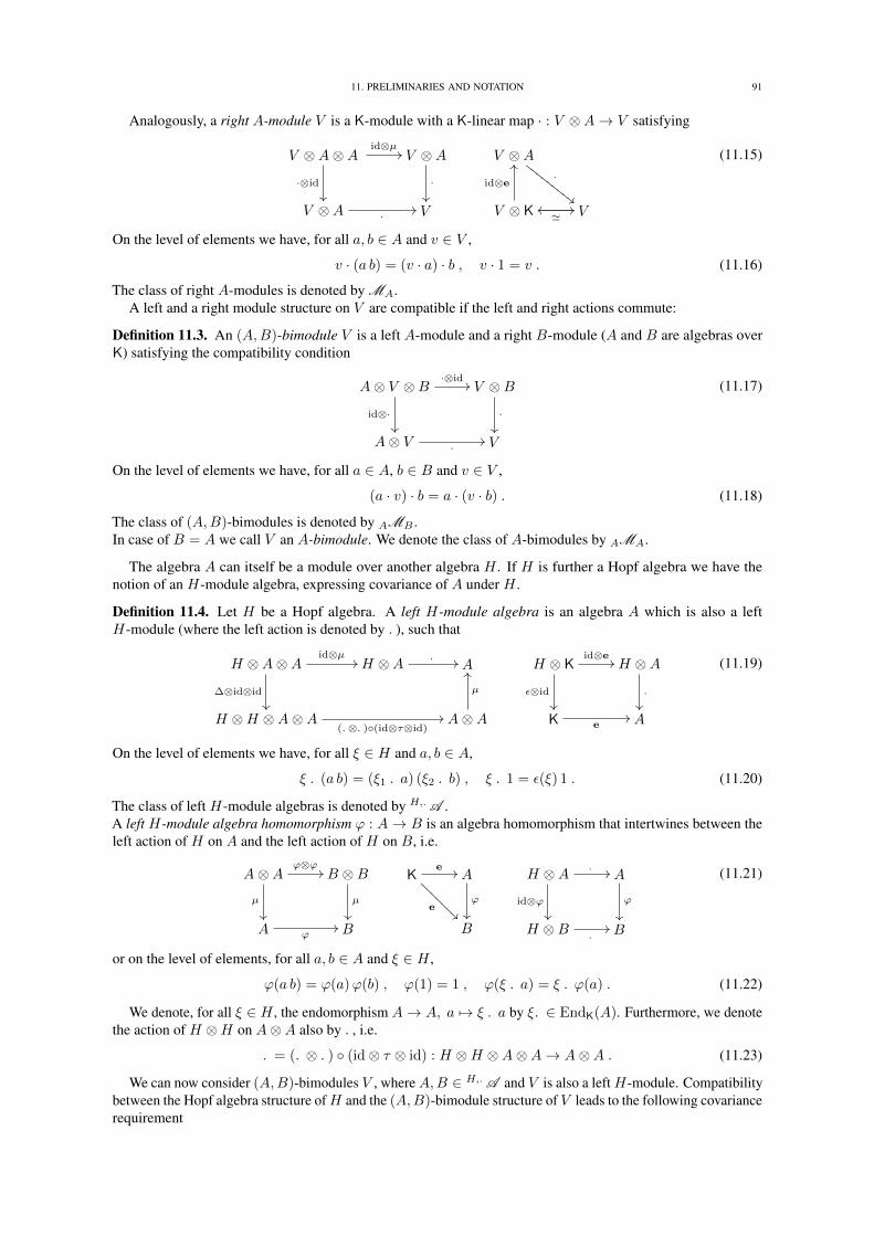
11. PRELIMINARIES AND NOTATION 91

Analogously, a right A-module V is a K-module with a K-linear map · : V ⊗A→ V satisfying

V ⊗A⊗A

·⊗id

id⊗µ// V ⊗A

·

V ⊗A ·// V

V ⊗A·

""FFFF

FFFF

F

V ⊗ K

id⊗e

OO

'// Voo

(11.15)

On the level of elements we have, for all a, b ∈ A and v ∈ V ,

v · (a b) = (v · a) · b , v · 1 = v . (11.16)

The class of right A-modules is denoted by MA.A left and a right module structure on V are compatible if the left and right actions commute:

Definition 11.3. An (A,B)-bimodule V is a left A-module and a right B-module (A and B are algebras overK) satisfying the compatibility condition

A⊗ V ⊗B·⊗id

//

id⊗·

V ⊗B

·

A⊗ V ·// V

(11.17)

On the level of elements we have, for all a ∈ A, b ∈ B and v ∈ V ,

(a · v) · b = a · (v · b) . (11.18)

The class of (A,B)-bimodules is denoted by AMB .In case of B = A we call V an A-bimodule. We denote the class of A-bimodules by AMA.

The algebra A can itself be a module over another algebra H . If H is further a Hopf algebra we have thenotion of an H-module algebra, expressing covariance of A under H .

Definition 11.4. Let H be a Hopf algebra. A left H-module algebra is an algebra A which is also a leftH-module (where the left action is denoted by .), such that

H ⊗A⊗Aid⊗µ

//

∆⊗id⊗id

H ⊗A . // A

H ⊗H ⊗A⊗A(.⊗.)(id⊗τ⊗id)

// A⊗A

µ

OO H ⊗ Kid⊗e

//

ε⊗id

H ⊗A

.

K e// A

(11.19)

On the level of elements we have, for all ξ ∈ H and a, b ∈ A,

ξ . (a b) = (ξ1 . a) (ξ2 . b) , ξ . 1 = ε(ξ) 1 . (11.20)

The class of left H-module algebras is denoted by H,.A .A left H-module algebra homomorphism ϕ : A→ B is an algebra homomorphism that intertwines between theleft action of H on A and the left action of H on B, i.e.

A⊗Aϕ⊗ϕ

//

µ

B ⊗Bµ

A ϕ// B

Ke //

e

@@@@

@@@ A

ϕ

B

H ⊗A . //

id⊗ϕ

A

ϕ

H ⊗B .// B

(11.21)

or on the level of elements, for all a, b ∈ A and ξ ∈ H ,

ϕ(a b) = ϕ(a)ϕ(b) , ϕ(1) = 1 , ϕ(ξ . a) = ξ . ϕ(a) . (11.22)

We denote, for all ξ ∈ H , the endomorphism A→ A, a 7→ ξ . a by ξ. ∈ EndK(A). Furthermore, we denotethe action of H ⊗H on A⊗A also by ., i.e.

. = (.⊗ .) (id⊗ τ ⊗ id) : H ⊗H ⊗A⊗A→ A⊗A . (11.23)

We can now consider (A,B)-bimodules V , whereA,B ∈ H,.A and V is also a leftH-module. Compatibilitybetween the Hopf algebra structure ofH and the (A,B)-bimodule structure of V leads to the following covariancerequirement

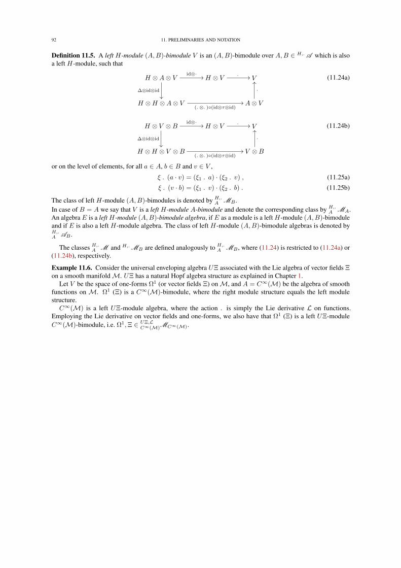
92 11. PRELIMINARIES AND NOTATION

Definition 11.5. A left H-module (A,B)-bimodule V is an (A,B)-bimodule over A,B ∈ H,.A which is alsoa left H-module, such that

H ⊗A⊗ Vid⊗·

//

∆⊗id⊗id

H ⊗ V . // V

H ⊗H ⊗A⊗ V(.⊗.)(id⊗τ⊗id)

// A⊗ V

·

OO(11.24a)

H ⊗ V ⊗Bid⊗·

//

∆⊗id⊗id

H ⊗ V . // V

H ⊗H ⊗ V ⊗B(.⊗.)(id⊗τ⊗id)

// V ⊗B

·

OO(11.24b)

or on the level of elements, for all a ∈ A, b ∈ B and v ∈ V ,

ξ . (a · v) = (ξ1 . a) · (ξ2 . v) , (11.25a)

ξ . (v · b) = (ξ1 . v) · (ξ2 . b) . (11.25b)

The class of left H-module (A,B)-bimodules is denoted by H,.A MB .

In case of B = A we say that V is a left H-module A-bimodule and denote the corresponding class by H,.A MA.

An algebra E is a left H-module (A,B)-bimodule algebra, if E as a module is a left H-module (A,B)-bimoduleand if E is also a left H-module algebra. The class of left H-module (A,B)-bimodule algebras is denoted byH,.A AB .

The classes H,.A M and H,.MB are defined analogously to H,.A MB , where (11.24) is restricted to (11.24a) or

(11.24b), respectively.

Example 11.6. Consider the universal enveloping algebra UΞ associated with the Lie algebra of vector fields Ξon a smooth manifoldM. UΞ has a natural Hopf algebra structure as explained in Chapter 1.

Let V be the space of one-forms Ω1 (or vector fields Ξ) onM, and A = C∞(M) be the algebra of smoothfunctions on M. Ω1 (Ξ) is a C∞(M)-bimodule, where the right module structure equals the left modulestructure.C∞(M) is a left UΞ-module algebra, where the action . is simply the Lie derivative L on functions.

Employing the Lie derivative on vector fields and one-forms, we also have that Ω1 (Ξ) is a left UΞ-moduleC∞(M)-bimodule, i.e. Ω1,Ξ ∈ UΞ,L

C∞(M)MC∞(M).

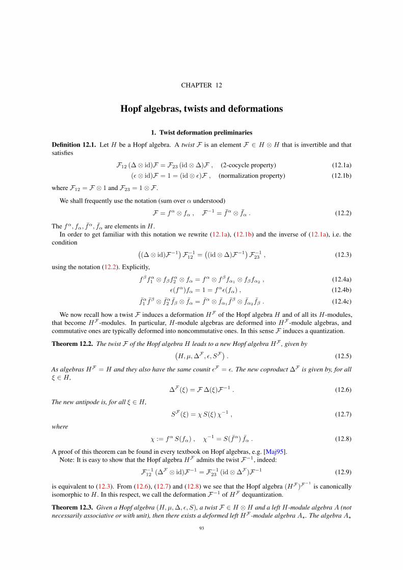
CHAPTER 12

Hopf algebras, twists and deformations

1. Twist deformation preliminaries

Definition 12.1. Let H be a Hopf algebra. A twist F is an element F ∈ H ⊗ H that is invertible and thatsatisfies

F12 (∆⊗ id)F = F23 (id⊗∆)F , (2-cocycle property) (12.1a)

(ε⊗ id)F = 1 = (id⊗ ε)F , (normalization property) (12.1b)

where F12 = F ⊗ 1 and F23 = 1⊗F .

We shall frequently use the notation (sum over α understood)

F = fα ⊗ fα , F−1 = fα ⊗ fα . (12.2)

The fα, fα, fα, fα are elements in H .In order to get familiar with this notation we rewrite (12.1a), (12.1b) and the inverse of (12.1a), i.e. the

condition ((∆⊗ id)F−1

)F−1

12 =((id⊗∆)F−1

)F−1

23 , (12.3)

using the notation (12.2). Explicitly,

fβfα1 ⊗ fβfα2 ⊗ fα = fα ⊗ fβfα1⊗ fβfα2

, (12.4a)

ε(fα)fα = 1 = fαε(fα) , (12.4b)

fα1 fβ ⊗ fα2 fβ ⊗ fα = fα ⊗ fα1

fβ ⊗ fα2fβ . (12.4c)

We now recall how a twist F induces a deformation HF of the Hopf algebra H and of all its H-modules,that become HF -modules. In particular, H-module algebras are deformed into HF -module algebras, andcommutative ones are typically deformed into noncommutative ones. In this sense F induces a quantization.

Theorem 12.2. The twist F of the Hopf algebra H leads to a new Hopf algebra HF , given by(H,µ,∆F , ε, SF

). (12.5)

As algebras HF = H and they also have the same counit εF = ε. The new coproduct ∆F is given by, for allξ ∈ H ,

∆F (ξ) = F ∆(ξ)F−1 . (12.6)

The new antipode is, for all ξ ∈ H ,

SF (ξ) = χS(ξ)χ−1 , (12.7)

where

χ := fα S(fα) , χ−1 = S(fα) fα . (12.8)

A proof of this theorem can be found in every textbook on Hopf algebras, e.g. [Maj95].Note: It is easy to show that the Hopf algebra HF admits the twist F−1, indeed:

F−112 (∆F ⊗ id)F−1 = F−1

23 (id⊗∆F )F−1 (12.9)

is equivalent to (12.3). From (12.6), (12.7) and (12.8) we see that the Hopf algebra (HF )F−1

is canonicallyisomorphic to H . In this respect, we call the deformation F−1 of HF dequantization.

Theorem 12.3. Given a Hopf algebra (H,µ,∆, ε, S), a twist F ∈ H ⊗H and a left H-module algebra A (notnecessarily associative or with unit), then there exists a deformed left HF -module algebra A?. The algebra A?

93

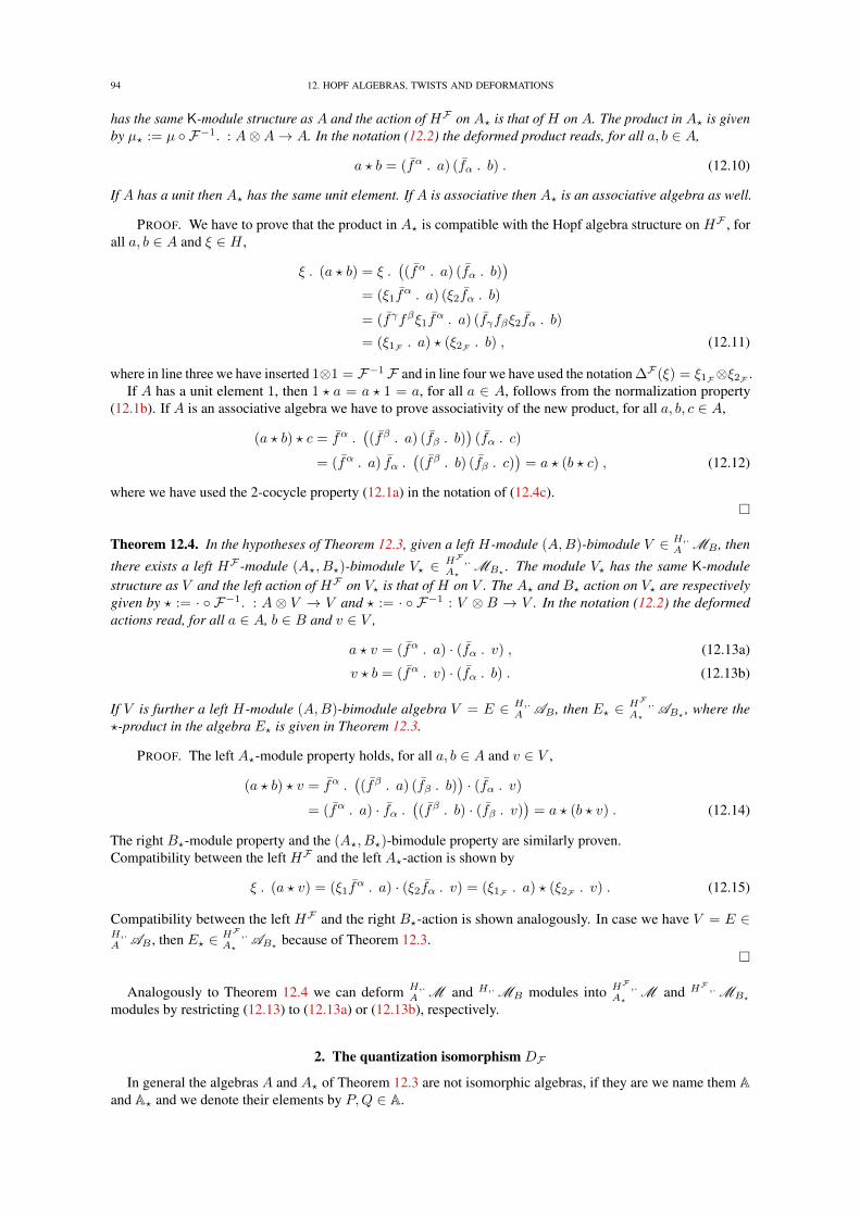
94 12. HOPF ALGEBRAS, TWISTS AND DEFORMATIONS

has the same K-module structure as A and the action of HF on A? is that of H on A. The product in A? is givenby µ? := µ F−1. : A⊗A→ A. In the notation (12.2) the deformed product reads, for all a, b ∈ A,

a ? b = (fα . a) (fα . b) . (12.10)

If A has a unit then A? has the same unit element. If A is associative then A? is an associative algebra as well.

PROOF. We have to prove that the product in A? is compatible with the Hopf algebra structure on HF , forall a, b ∈ A and ξ ∈ H ,

ξ . (a ? b) = ξ .((fα . a) (fα . b)

)= (ξ1f

α . a) (ξ2fα . b)

= (fγfβξ1fα . a) (fγfβξ2fα . b)

= (ξ1F . a) ? (ξ2F . b) , (12.11)

where in line three we have inserted 1⊗1 = F−1 F and in line four we have used the notation ∆F (ξ) = ξ1F⊗ξ2F .If A has a unit element 1, then 1 ? a = a ? 1 = a, for all a ∈ A, follows from the normalization property

(12.1b). If A is an associative algebra we have to prove associativity of the new product, for all a, b, c ∈ A,

(a ? b) ? c = fα .((fβ . a) (fβ . b)

)(fα . c)

= (fα . a) fα .((fβ . b) (fβ . c)

)= a ? (b ? c) , (12.12)

where we have used the 2-cocycle property (12.1a) in the notation of (12.4c).

Theorem 12.4. In the hypotheses of Theorem 12.3, given a left H-module (A,B)-bimodule V ∈ H,.A MB , then

there exists a left HF -module (A?, B?)-bimodule V? ∈ HF ,.A?

MB? . The module V? has the same K-modulestructure as V and the left action of HF on V? is that of H on V . The A? and B? action on V? are respectivelygiven by ? := · F−1. : A ⊗ V → V and ? := · F−1 : V ⊗ B → V . In the notation (12.2) the deformedactions read, for all a ∈ A, b ∈ B and v ∈ V ,

a ? v = (fα . a) · (fα . v) , (12.13a)

v ? b = (fα . v) · (fα . b) . (12.13b)

If V is further a left H-module (A,B)-bimodule algebra V = E ∈ H,.A AB , then E? ∈ HF ,.

A?AB? , where the

?-product in the algebra E? is given in Theorem 12.3.

PROOF. The left A?-module property holds, for all a, b ∈ A and v ∈ V ,

(a ? b) ? v = fα .((fβ . a) (fβ . b)

)· (fα . v)

= (fα . a) · fα .((fβ . b) · (fβ . v)

)= a ? (b ? v) . (12.14)

The right B?-module property and the (A?, B?)-bimodule property are similarly proven.Compatibility between the left HF and the left A?-action is shown by

ξ . (a ? v) = (ξ1fα . a) · (ξ2fα . v) = (ξ1F . a) ? (ξ2F . v) . (12.15)

Compatibility between the left HF and the right B?-action is shown analogously. In case we have V = E ∈H,.A AB , then E? ∈ HF ,.

A?AB? because of Theorem 12.3.

Analogously to Theorem 12.4 we can deform H,.A M and H,.MB modules into HF ,.

A?M and HF ,.MB?

modules by restricting (12.13) to (12.13a) or (12.13b), respectively.

2. The quantization isomorphism DF

In general the algebras A and A? of Theorem 12.3 are not isomorphic algebras, if they are we name them Aand A? and we denote their elements by P,Q ∈ A.

2. THE QUANTIZATION ISOMORPHISM DF 95

Theorem 12.5. Let A be a left H-module algebra (not necessarily associative or with unit) and also a rightmodule with respect to the algebra (H,µ) (the right action of (H,µ) on A is simply denoted by juxtaposition),with the compatibility conditions, for all P,Q ∈ A and ξ, η ∈ H ,

(PQ)ξ = P (Qξ) , (12.16a)

(Pξ)Q = P (ξ1 . Q)ξ2 , (12.16b)

ξ . (Pη) = (ξ1 . P )(ξ2 . η) , (12.16c)

where ξ . η = ξ1 η S(ξ2) is the adjoint action of H on H . In this case the algebras A and A? are isomorphicalgebras.

Before proving this theorem notice that A in the hypotheses above is a left module with respect to the algebra(H,µ) by defining, for all ξ ∈ H and P ∈ A,

ξP := (ξ1 . P )ξ2 . (12.17)

Indeed, we have for all ξ, η ∈ H and P ∈ A

ξ(ηP ) = ξ((η1 . P )η2

)=(ξ1 .

((η1 . P )η2

))ξ2 = (ξ1η1 . P )(ξ2 . η2)ξ3

= (ξ1η1 . P )ξ2η2S(ξ3)ξ4 = (ξ1η1 . P )ξ2η2 = (ξη)P . (12.18)

Moreover, A is an (H,µ)-bimodule, i.e. we have for all ξ, η ∈ H and P ∈ A,

ξ(Pη) =(ξ1 . (Pη)

)ξ2 =

((ξ1 . P )(ξ2 . η)

)ξ3 = (ξ1 . P )ξ2ηS(ξ3)ξ4 = (ξP )η . (12.19)

The Hopf algebra action . on A is just the adjoint action with respect to this bimodule structure

ξ . P = ξ1PS(ξ2) . (12.20)

Condition (12.16b) then simply reads

(Pξ)Q = P (ξQ) , (12.21)

for all P,Q ∈ A and ξ ∈ H . We obtain for the left (H,µ)-action, for all ξ ∈ H and P,Q ∈ A,

ξ(PQ) = (ξP )Q . (12.22)

In case A is unital with 1A ∈ A we also find, for all ξ ∈ H ,

ξ1A = (ξ1 . 1A)ξ2 = 1Aε(ξ1)ξ2 = 1Aξ . (12.23)

Vice versa, if A is an algebra and an (H,µ)-bimodule satisfying (12.16a), (12.21) and (12.22) (as well as(12.23) in case A is unital), then ξ .P := ξ1 PS(ξ2) defines a leftH-module structure on A that satisfies (12.16b)and (12.16c). Hence, Theorem 12.5 equivalently reads

Theorem 12.6. Consider a Hopf algebra H and an (H,µ)-bimodule A that is also an algebra (not necessarilyassociative or with unit). If, for all ξ ∈ H and P,Q ∈ A, the “generalized associativity” conditions

(PQ)ξ = P (Qξ) , (Pξ)Q = P (ξQ) , ξ(PQ) = (ξP )Q , (12.24a)

and in case of A unital also the condition

ξ1A = 1Aξ , (12.24b)

hold true, then the adjoint action (12.20) structures A as a left module algebra with respect to the Hopf algebraH . Given a twist F of the Hopf algebra H , the twist quantized algebra A? is isomorphic to A, via the map

DF : A? → A , P 7→ DF (P ) = (fα . P )fα = fα1 PS(fα2 )fα . (12.25)

PROOF. DF is obviously a K-linear map. We prove that

DF µ? = µ (DF ⊗DF ) , (12.26)

for all P,Q ∈ A,

DF (P ? Q) = DF((fβ . P )(fβ . Q)

)=(fα .

((fβ . P )(fβ . Q)

))fα

= (fα1 fβ . P )(fα2 fβ . Q)fα = (fα . P )(fα1

fβ . Q)fα2fβ

= (fα . P )fα (fβ . Q)fβ = DF (P )DF (Q) , (12.27)

where in the second equality in the second line we have used (12.4c) and in the first equality in the third line wehave used

(fα1fβ . Q)fα2

= fα1(fβ . Q)S(fα2

)fα3= fα(fβ . Q) . (12.28)

96 12. HOPF ALGEBRAS, TWISTS AND DEFORMATIONS

This shows that DF is an algebra homomorphism and it remains to prove its invertability. We can simplify(12.25) by using (12.4) as follows

DF (P ) = fα1 PS(fα2 )fα = fαfγPS(fα1 fβfγ)fα2 fβ

= fαfγPS(fγ)S(fβ)ε(fα)fβ = fγPS(fγ)χ−1 , (12.29)

where χ−1 = S(fα)fα. Therefore, DF is invertible and we have for all P ∈ A

D−1F (P ) = fαPχS(fα) , (12.30)

where χ = fβS(fβ).Finally, if A is unital, DF maps the unit of A? to the unit of A because of the normalization property of the

twist (12.1b),

DF (1A) = (fα . 1A)fα = 1Aε(fα)fα = 1A1 = 1A . (12.31)

In the hypotheses of Theorem 12.6, the Hopf algebra properties immediately imply that the algebra A has aleft HF -module algebra structure given by the adjoint HF -action, for all ξ ∈ H and P ∈ A,

ξ .F P := ξ1FPSF (ξ2F ) . (12.32)

Theorem 12.7. The algebra isomorphism DF : A? → A of Theorem 12.6 is also an isomorphism betweenthe left HF -module algebra A? ∈ HF ,.A and the left HF -module algebra A ∈ HF ,.FA , i.e. DF intertwinesbetween the left HF -actions . and .F , for all ξ ∈ H and P ∈ A,

DF (ξ . P ) = ξ .F DF (P ) . (12.33)

PROOF. Using (12.29) we obtain

DF (ξ . P ) = fβ(ξ . P )S(fβ)χ−1 = fβξ1PS(fβξ2)χ−1 = ξ1F fβPS(ξ2F fβ)χ−1

= ξ1F fβPS(fβ)χ−1χS(ξ2F )χ−1 = ξ1FDF (P )SF (ξ2F ) = ξ .F DF (P ) . (12.34)

Remark 12.8. We have discussed above that HF admits the twist F−1 leading to (HF )F−1

= H . Theassociated quantization isomorphism is exactly D−1

F given in (12.30). This can be shown by using (12.29) and ashort calculation, for all P ∈ A,

(fα .F P )fα = fαPSF (fα)χ−1F = fαPχS(fα)χ−1χ = D−1

F (P ) , (12.35)

where we have used that χ−1F = SF (fα)fα = χ.

In order to show that algebras of the type A actually appear quite naturally we provide some examples.

Example 12.9. Given a left H-module algebra A (not necessarily associative or with unit) consider the crossedproduct (or smash product) A]H . By definition the underlying K-module of A]H is A⊗H , and the product isgiven by

(a⊗ ξ)(b⊗ η) = a(ξ1 . b)⊗ ξ2η . (12.36)

Note that in case A is associative, then so is A]H , and that in case A is unital, then so is A]H with unit1A ⊗ 1H . The algebra A]H is a left H-module algebra with the action ξ . (a⊗ η) = (ξ1 . a)⊗ (ξ2 . η). Theright (H,µ)-module structure is given by (a⊗ ξ)η = a⊗ (ξη) and the compatibility conditions (12.16) holdtrue. Hence, the requirements of Theorem 12.5 are satisfied. Notice that A is always a subalgebra of A]H viaa 7→ a⊗ 1H , for all a ∈ A. If A is unital, then H is also a subalgebra of A]H via ξ 7→ 1A ⊗ ξ, for all ξ ∈ H .

Example 12.10. Given an associative and unital algebra A that admits a homomorphism ρ : H → A, then thehypotheses of Theorem 12.6 immediately hold, just define the (H,µ)-bimodule structure of A by, for all ξ ∈ Hand P ∈ A, ξP := ρ(ξ)P and Pξ := Pρ(ξ). A particular case is when A = H and we consider the identityhomomorphism. Then we recover the (Hopf algebra) isomorphism D : H? → HF discussed in Chapter 1,Section 4, see also [GM94, ADMW06].

Example 12.11. Given a Hopf algebra H over the ring K and a left H-module V , consider the algebra EndK(V )of K-linear maps (K-module homomorphisms) from V to V . Since H is a Hopf algebra the left action of H onV lifts to a left action of H on EndK(V ), defined by, for all ξ ∈ H and P ∈ EndK(V ),

ξ I P := ξ1 . P S(ξ2). , (12.37)

2. THE QUANTIZATION ISOMORPHISM DF 97

where denotes the usual composition of morphisms and ξ. ∈ EndK(V ) the endomorphism v 7→ ξ . v. Thealgebra EndK(V ) is thus a left H-module algebra, i.e. EndK(V ) ∈ H,IA . The algebra homomorphism H →EndK(V ) , ξ 7→ ξ. implies, by using the previous example, the isomorphism DF : EndK(V )? → EndK(V ),where the composition law in EndK(V )? is given by the ?-composition, for all P,Q ∈ EndK(V )?,

P ? Q := (fα I P ) (fα I Q) . (12.38)

By Theorem 12.7 we even obtain a left HF -module algebra isomorphism DF between EndK(V )? ∈ HF ,IA

and EndK(V ) ∈ HF ,IFA .

CHAPTER 13

Module homomorphisms

1. Quantization of endomorphisms

In this section we study the algebras EndK(V ) and EndB(V ) of endomorphisms of a module V ∈ H,.A MB .

We then investigate how they behave under twist quantization.

Proposition 13.1. Let A ∈ H,.A and V ∈ H,.A M , then the algebra EndK(V ) of K-linear maps from V to V is

a left H-module A-bimodule algebra

EndK(V ) ∈ H,IA AA , (13.1)

where I is the adjoint H-action, for all ξ ∈ H and P ∈ EndK(V ),

ξ I P := ξ1 . P S(ξ2). , (13.2)

and the A-bimodule structure is given by, for all a ∈ A and P ∈ EndK(V ),

a · P := la P , (13.3a)P · a := P la , (13.3b)

where, for all v ∈ V , la(v) := a · v.If V is also a right module over B ∈ H,.A , such that V ∈ H,.

A MB , then the subalgebra of right B-linearendomorphisms of V , EndB(V ) ⊆ EndK(V ), is still a left H-module A-bimodule algebra

EndB(V ) ∈ H,IA AA , (13.4)

with H and A actions given in (13.2) and (13.3), respectively.

PROOF. EndK(V ) is an A-bimodule, since for all a, b ∈ A and P ∈ EndK(V ),

a · (b · P ) = la (lb P ) = lab P = (ab) · P ,

(P · a) · b = (P la) lb = P lab = P · (ab) ,a · (P · b) = la (P lb) = (la P ) lb = (a · P ) · b . (13.5)

It is straightforward to check that EndK(V ) is a left H-module algebra, for all ξ, η ∈ H and P,Q ∈ EndK(V ),

ξ I (η I P ) = (ξη) I P , ξ I idV = ε(ξ) idV , (13.6)

and

ξ I (P Q) = (ξ1 I P ) (ξ2 I Q) . (13.7)

In order to show that EndK(V ) is a left H-module A-bimodule algebra it remains to prove the compatibilitiesξ I (a · P ) = (ξ1 . a) · (ξ2 I P ) and ξ I (P · a) = (ξ1 I P ) · (ξ2 . a). They immediately follow from (13.7)and ξ I la = lξ.a, for all ξ ∈ H and a ∈ A. The latter property is simply shown to hold

(ξ I la)(v) = ξ1 .(la(S(ξ2) . v)

)= ξ1 .

(a · (S(ξ2) . v)

)= (ξ1 . a) · (ξ2S(ξ3) . v) = (ξ . a) · v = lξ.a(v) , (13.8)

for all v ∈ V .Finally, let V ∈ H,.

A MB , then (by definition) V is an (A,B)-bimodule and we in particular have a · (v · b) =(a · v) · b, hence la ∈ EndB(V ) for all a ∈ A. Therefore, a ·P ∈ EndB(V ) and P · a ∈ EndB(V ) for all a ∈ Aand P ∈ EndB(V ). Furthermore, for all ξ ∈ H and P ∈ EndB(V ) we have ξ I P ∈ EndB(V ), since

(ξ I P )(v · b) = ξ1 .(P((S(ξ3) . v) · (S(ξ2) . b)

))=(ξ1 .

(P (S(ξ4) . v)

))·(ξ2 .

(S(ξ3) . b

))= (ξ I P )(v) · b , (13.9)

for all v ∈ V and b ∈ B.

99

100 13. MODULE HOMOMORPHISMS

Let H be a Hopf algebra with twist F ∈ H ⊗ H , and let A,B ∈ H,.A , V ∈ H,.A MB . As a conse-

quence, EndK(V ),EndB(V ) ∈ H,IA AA. We have two possible deformations of the endomorphisms EndK(V ),

EndB(V ): The first, EndK(V )?,EndB(V )? ∈ HF ,IA?

AA? is obtained by applying Theorem 12.4 to the leftH-module A-bimodule algebras EndK(V ), EndB(V ). It is characterized by a deformed composition lawP ? Q = (fα I P ) (fα I Q). The second option is simply to consider the K-linear or right B?-linear endo-morphisms of the deformed module V?. From Proposition 13.1 we have EndK(V?),EndB?(V?) ∈ HF ,IF

A?AA? .

Here the product is the usual composition law and the action is the adjoint HF -action, for all ξ ∈ HF andP ∈ EndK(V?),

ξ IF P := ξ1F . P SF (ξ2F ) . . (13.10)

Theorem 13.2. The map

DF : EndK(V )? → EndK(V?) , P 7→ DF (P ) = (fα I P ) fα. (13.11)

is an isomorphism between the leftHF -moduleA?-bimodule algebras EndK(V )? ∈ HF ,IA?

AA? and EndK(V?) ∈HF ,IFA?

AA? . It restricts to a left HF -module A?-bimodule algebra isomorphism

DF : EndB(V )? → EndB?(V?) . (13.12)

We call DF (P ) the quantization of the endomorphism P ∈ EndB(V ).

PROOF. Since V = V? as HF -modules, we have as left HF -module algebras EndK(V?) = EndK(V ).The left HF -module algebra isomorphism (13.11) is therefore the isomorphism DF : EndK(V )? → EndK(V )discussed in Example 12.11.

The A?-bimodule structure of EndK(V )? is given by (cf. Theorem 12.4), for all a ∈ A and P ∈ EndK(V ),

a ? P := lfα.a (fα I P ) = (fα I la) (fα I P ) = la ? P , (13.13a)

P ? a := (fα I P ) lfα.a = (fα I P ) (fα I la) = P ? la . (13.13b)

The A?-bimodule structure of EndK(V?) is given by (cf. Proposition 13.1), for all a ∈ A? and P? ∈ EndK(V?),

aFP? := l?a P? , (13.14a)

P?Fa := P? l?a , (13.14b)

where, for all v ∈ V?, l?a(v) := a ? v. The map DF is a left HF -module A?-bimodule algebra isomorphism,because (cf. Theorem 12.6) DF (a ? P ) = DF (la ? P ) = DF (la) DF (P ), DF (P ? a) = DF (P ) DF (la)and DF (la) = l?a. The last property follows from a short calculation

DF (la)(v) = (fα I la)(fα . v) = lfα.a(fα . v) = a ? v = l?a(v) , (13.15)

for all v ∈ V .In order to show that DF restricts to an isomorphism between the left HF -module A?-bimodule subalgebrasEndB(V )? ∈ HF ,I

A?AA? and EndB?(V?) ∈ HF ,IF

A?AA? , we have to prove that for all P ∈ EndB(V ) we have

DF (P ) ∈ EndB?(V?) and that for all P? ∈ EndB?(V?) we have D−1F (P?) ∈ EndB(V ). Employing Remark

12.8 it is sufficient to prove the first statement, since the second follows from dequantization with F−1. Weobtain by a short calculation, for all v ∈ V and b ∈ B,

DF (P )(v ? b) = (fα I P )((fα1

fβ . v) · (fα2fβ . b)

)= (fα1 f

β I P )(fα2 fβ . v

)· (fα . b)

= fα .(DF (P )(v)

)· (fα . b) = DF (P )(v) ? b , (13.16)

where in the second line we have used the 2-cocycle property of the twist (12.4c) and the fact that ξ I P ∈EndB(V ) for all ξ ∈ H and P ∈ EndB(V ).

We have so far studied right B-linear endomorphisms EndB(V ), but we as well could have studied leftA-linear endomorphisms AEnd(V ) of V ∈ H,.

A MB . These are related to the right linear endomorphisms by a“mirror” construction.

Recall that given a Hopf algebra (H,µ,∆, ε, S) with an invertible antipode S, we have the Hopf algebrasHcop and Hop. With an abuse of notation denoting also the underlying K-module by H , we have explicitlyHcop = (H,µ,∆cop, ε, S−1) and Hop = (H,µop,∆, ε, S

−1), where the coopposite coproduct is defined by,for all ξ ∈ H , ∆cop(ξ) = ξ1cop ⊗ ξ2cop = ξ2 ⊗ ξ1, and the opposite product is given by, for all ξ, η ∈ H ,µop(ξ ⊗ η) = µ(η ⊗ ξ) = η ξ. Note that Hcop

op = (H,µop,∆cop, ε, S) even exists when S is not invertible. For

1. QUANTIZATION OF ENDOMORPHISMS 101

a simplified mirror construction based on Hcop (and not on Hcopop ) we are going to assume from now on that

S−1 exists. This assumption is motivated by the fact that S−1 exists, in particular, for all quasitriangular Hopfalgebras (see e.g. [Maj95]), which will be the main subject of our studies.

We observe that for any left module V ∈ AM there is a right module V op ∈MAop . As K-modules V = V op,the algebra Aop is the algebra with opposite product and its right action on V op is given by v ·op a := a · v.Similarly, for any right module V ∈MA there is a left module V op ∈ AopM , and (V op)op = V .

Moreover, if we have a left H-module algebra A ∈ H,.A then the opposite algebra is a left Hcop-modulealgebra

A ∈ H,.A =⇒ Aop ∈ Hcop,.A , (13.17)

where the Hopf algebra action is unchanged. This easily leads to the following

Lemma 13.3. Let A,B ∈ H,.A and V ∈ H,.A MB , then Aop, Bop ∈ Hcop,.A and V op ∈ Hcop,.

Bop MAop . IfE ∈ H,.

A AB , then Eop ∈ Hcop,.Bop AAop .

We apply these observations to the algebra of endomorphisms of the module V and obtain

Proposition 13.4. Let A,B ∈ H,.A and V ∈ H,.A MB , then

(AEnd(V )

)op ∈ H,Icop

B AB , where for all ξ ∈ Hand P ∈ AEnd(V ),

ξ Icop P := ξ2 . P S−1(ξ1). , (13.18)

i.e. the action Icop is just the adjoint action of Hcop, ξ Icop P = ξ1cop . P Scop(ξ2cop). .

PROOF. The hypothesis and Lemma 13.3 implies Aop, Bop ∈ Hcop,.A , V op ∈ Hcop,.Bop MAop , and hence

EndAop(V op) ∈ Hcop,Icop

Bop ABop . Because of Lemma 13.3 we have(EndAop(V op)

)op ∈ H,Icop

B AB . The prooffollows by using the canonical algebra isomorphism

EndAop(V op) ' AEnd(V ) (13.19)

given by the identity map. Indeed, if P ∈ EndAop(V op), then for all a ∈ A and v ∈ V ,

P (a · v) = P (v ·op a) = P (v) ·op a = a · P (v) , (13.20)

hence P ∈ AEnd(V ), and vice versa.

The B-bimodule structure of(AEnd(V )

)opexplicitly reads, for all b ∈ B and P ∈ AEnd(V ),

b · P = P lopb = P rb , P · b = lop

b P = rb P , (13.21)

where, for all v ∈ V , rb(v) := v · b.Similar to Theorem 13.2 we have a left quantization map.

Theorem 13.5. Let H be a Hopf algebra with twist F ∈ H ⊗H , and let A,B ∈ H,.A , V ∈ H,.A MB . The map

DcopF :

((AEnd(V )

)op)?→(A?End(V?)

)op, P 7→ Dcop

F (P ) = (fα Icop P ) fα. (13.22)

is an isomorphism between the left HF -module B?-bimodule algebras((AEnd(V )

)op)?∈ HF ,Icop

B?AB? and(

A?End(V?))op ∈ HF ,(IF )cop

B?AB? .

We call DcopF (P ) the left quantization of the endomorphism P ∈ AEnd(V ).

PROOF. Recall that if F is a twist ofH , then Fcop = F21 is a twist of the Hopf algebraHcop. From Lemma13.3, Proposition 13.1, and the Theorems 12.3 and 12.4 we have(

EndAop(V op))?cop ∈

(Hcop)Fcop

,Icop

(Bop)?copA(Bop)?cop , (13.23a)

and

End(Aop)?cop ((V op)?cop) ∈ (Hcop)Fcop

,(Icop)Fcop

(Bop)?copA(Bop)?cop , (13.23b)

where ?cop is the ?-product of Fcop. Theorem 13.2 implies the left (Hcop)Fcop

-module (Bop)?cop-bimodulealgebra isomorphism

DFcop = DcopF :

(EndAop(V op)

)?cop → End(Aop)?cop ((V op)?cop) . (13.24)

Observe that

(Aop)?cop = (A?)op , (Bop)?cop = (B?)

op , (V op)?cop = (V?)op , (13.25a)

102 13. MODULE HOMOMORPHISMS

as well as

(Hcop)Fcop

= (HF )cop , (Icop)Fcop = (IF )cop . (13.25b)

Using the canonical algebra isomorphism EndAop(V op) ' AEnd(V ) we have(EndAop(V op)

)?cop '

(AEnd(V )

)?cop =

((AEnd(V )

)op op)?cop =

((AEnd(V )

)op) op

?(13.26a)

and

End(Aop)?cop ((V op)?cop) = End(A?)op((V?)op) ' A?End(V?) . (13.26b)

The proof of the theorem follows by applying Lemma 13.3 to (13.24), leading to the leftHF -moduleB?-bimodulealgebra isomorphism (13.22).

2. Quantization of homomorphisms

Let H be a Hopf algebra, A,B ∈ H,.A and V,W ∈ H,.A M . In this section we focus on K-linear maps from

V to W , denoted by HomK(V,W ), and their quantization. In case of V,W ∈ H,.A MB , we can also consider

right B-linear homomorphisms HomB(V,W ) from V to W . Properties of left A-linear homomorphismsAHom(V,W ) and their quantization will follow from a mirror construction. The results are analogous to thosefor the endomorphisms above. For completeness and for a better overview we will briefly present the mainpropositions and theorems.

Proposition 13.6. Let A ∈ H,.A and V,W ∈ H,.A M , then the K-module HomK(V,W ) of K-linear maps from

V to W is a left H-module A-bimodule

HomK(V,W ) ∈ H,IA MA , (13.27)

where I is the adjoint H-action, for all ξ ∈ H and P ∈ HomK(V,W ),

ξ I P := ξ1 . P S(ξ2). , (13.28)

and the A-bimodule structure is given by, for all a ∈ A and P ∈ HomK(V,W ),

a · P := la P , (13.29a)P · a := P la , (13.29b)

where we used for notational simplicity the same symbol la for the left multiplication map on V and W .If V,W are also right B-modules, such that V,W ∈ H,.

A MB , then the K-submodule of right B-linear homomor-phisms, HomB(V,W ) ⊆ HomK(V,W ), is still a left H-module A-bimodule

HomB(V,W ) ∈ H,IA MA , (13.30)

with H and A actions given in (13.28) and (13.29), respectively.

The proof of this proposition is analogous to Proposition 13.1 so that we can omit it here.Let now H be a Hopf algebra with twist F ∈ H ⊗ H , and let A,B ∈ H,.A , V,W ∈ H,.

A MB . Asa consequence, HomK(V,W ),HomB(V,W ) ∈ H,I

A MA. Analogously to the endomorphisms, we have twopossible deformations of the homomorphisms HomK(V,W ) and HomB(V,W ). The first option, HomK(V,W )?,HomB(V,W )? ∈ HF ,I

A?MA? , is obtained by applying Theorem 12.4. The second option, HomK(V?,W?),

HomB?(V?,W?) ∈ HF ,IFA?

MA? , is just to consider homomorphisms between the quantized modules V? and W?.Similar to Theorem 13.2 we can relate these two constructions.

Theorem 13.7. The map

DF : HomK(V,W )? → HomK(V?,W?) , P 7→ DF (P ) = (fα I P ) fα. (13.31)

is an isomorphism between the left HF -module A?-bimodules HomK(V,W )? ∈ HF ,IA?

MA? and

HomK(V?,W?) ∈ HF ,IFA?

MA? . It restricts to a left HF -module A?-bimodule isomorphism

DF : HomB(V,W )? → HomB?(V?,W?) . (13.32)

We call DF (P ) the quantization of the homomorphism P ∈ HomB(V,W ).

3. QUASI-COMMUTATIVE ALGEBRAS AND BIMODULES 103

Since the proof is analogous to the one of Theorem 13.2 we do not have to provide it here.For completeness, we also briefly discuss left A-linear homomorphisms AHom(V,W ) and their quantization.

We have(AHom(V,W )

)op ∈ H,Icop

B MB , where the left H-action is given by, for all ξ ∈ H and P ∈AHom(V,W ),

ξ Icop P := ξ2 . P S−1(ξ1). , (13.33a)

and the B-bimodule structure reads, for all b ∈ B and P ∈ AHom(V,W ),

b · P := P rb , P · b := rb P . (13.33b)

The quantization of left A-linear homomorphisms is understood analogously to Theorem 13.7.

Theorem 13.8. Let H be a Hopf algebra with twist F ∈ H ⊗H , and let A,B ∈ H,.A , V,W ∈ H,.A MB . The

map

DcopF :

((AHom(V,W )

)op)?→(A?Hom(V?,W?)

)op, P 7→ Dcop

F (P ) = (fα Icop P ) fα. (13.34)

is an isomorphism between the left HF -module B?-bimodules((AHom(V,W )

)op)?∈ HF ,Icop

B?MB? and(

A?Hom(V?,W?))op ∈ HF ,(IF )cop

B?MB? .

We call DcopF (P ) the left quantization of the homomorphism P ∈ AHom(V,W ).

This theorem can be proven with a mirror construction (analogously to Theorem 13.5), or equivalently by directa calculation.

Example 13.9. Let A ∈ H,.A and V ∈ H,.A MA. The dual module of V is defined by V ′ := HomA(V,A).

Since A can be regarded as a left H-module A-bimodule, we have by Proposition 13.6 V ′ ∈ H,IA MA. Let

F ∈ H ⊗ H be a twist of H and consider the deformed HF -modules A? ∈ HF ,.A and V? ∈ HF ,.A?

MA? .

We have two possible deformations of the dual module, (V ′)? = HomA(V,A)? ∈ HF ,IA?

MA? and (V?)′ =

HomA?(V?, A?) ∈ HF ,IFA?

MA? . Due to Theorem 13.7 there is a left HF -module A?-bimodule isomorphismDF , such that (V?)

′ ' (V ′)?. In words, dualizing the quantized module is (up to isomorphism) equivalentto quantizing the dual one. Note that by Theorem 13.8 similar statements hold true for the left A-linear dual′V =

(AHom(V,A)

)opand its quantization.

3. Quasi-commutative algebras and bimodules

In many examples Hopf algebras come with the additional structure of an R-matrix. In particular, all modelsfrom Part I and Part II fall into this class. This justifies to study properties of endomorphisms and homomorphismsin presence of this extra structure.

Definition 13.10. A quasi-cocommutative Hopf algebra (H,R) is a Hopf algebra H together with an invertibleelement R ∈ H ⊗H (called universal R-matrix) such that, for all ξ ∈ H ,

∆cop(ξ) = R∆(ξ)R−1 . (13.35)

A quasi-cocommutative Hopf algebra is called quasitriangular if

(∆⊗ id)R = R13R23 , (id⊗∆)R = R13R12 , (13.36)

and triangular if additionally

R21 = R−1 . (13.37)

Example 13.11. The Hopf algebra UΞ of diffeomorphisms of a manifoldM (see Chapter 1) is triangular withtrivial R-matrix R = 1 ⊗ 1. The twist deformation UΞF of UΞ is triangular with R-matrix RF = F21 F−1.Moreover, the twist deformation of any (quasi)triangular Hopf algebra (H,R) is (quasi)triangular with R-matrixRF = F21RF−1.

From the definition of a quasitriangular Hopf algebra the following standard properties follow (see e.g. [Maj95,Kas95])

(ε⊗ id)R = 1 , (id⊗ ε)R = 1 , (13.38a)

(S ⊗ id)R = R−1 , (id⊗ S)R−1 = R , (13.38b)

and

R12R13R23 = R23R13R12 . (13.38c)

104 13. MODULE HOMOMORPHISMS

Notice that the properties (13.36) and (13.38c) imply that R is a twist of the Hopf algebra H , and from (13.35)we obtain HR = Hcop. The Hopf algebra Hcop is quasitriangular with R-matrix R21.

Similar to the twist we introduce the notations R = Rα ⊗Rα and R−1 = Rα ⊗ Rα (sum over α understood).

Definition 13.12. Let (H,R) be a quasitriangular Hopf algebra. A left H-module algebra A ∈ H,.A is calledquasi-commutative if, for all a, b ∈ A,

a b = (Rα . b) (Rα . a) . (13.39)

Similarly, a left H-module A-bimodule V ∈ H,.A MA is quasi-commutative if, for all a ∈ A and v ∈ V ,

v · a = (Rα . a) · (Rα . v) . (13.40)

Note that as a consequence of (13.40) we have

a · v = (Rα . v) · (Rα . a) . (13.41)

Example 13.13. Consider the Hopf algebra of diffeomorphisms UΞ of a manifoldM. Then trivially the algebraof smooth functions C∞(M) is quasi-commutative, since it is commutative and R = 1 ⊗ 1. Furthermore,the C∞(M)-bimodules Ω1 and Ξ of one-forms and vector fields are quasi-commutative bimodules. Let Fbe a twist of UΞ. Then UΞF is triangular with R = F21F−1 and the deformed algebra (C∞(M), ?), aswell as the deformed bimodules Ω1

? and Ξ?, are quasi-commutative. In general, the twist quantization of anyquasi-commutative algebra or bimodule is quasi-commutative.

Proposition 13.14. Let (H,R) be a quasitriangular Hopf algebra and let A ∈ H,.A and V,W ∈ H,.A MA be

quasi-commutative. Then for all P ∈ HomA(V,W ), a ∈ A and v ∈ VP (a · v) = (Rα . a) · (Rα I P )(v) . (13.42)

Similarly, for all P ∈ AHom(V,W ), a ∈ A and v ∈ VP (v · a) = (Rα I

cop P )(v) · (Rα . a) . (13.43)

PROOF. We show (13.42), for all P ∈ HomA(V,W ), a ∈ A and v ∈ V ,

P (a · v) = P((Rα . v) · (Rα . a)

)= P (Rα . v) · (Rα . a)

= (RβRα . a) · Rβ .(P (Rα . v)

)= (RβRα . a) · Rβ .

(P (S(Rα) . v)

)= (Rα . a) · Rα1

.(P (S(Rα2

) . v))

= (Rα . a) · (Rα I P )(v) , (13.44)

where in line three we have used (13.38b) and in line four (13.36). The property (13.43) is proven analogously.

This immediately leads us to the following

Corollary 13.15. Let (H,R) be a quasitriangular Hopf algebra and letA ∈ H,.A and V,W ∈ H,.A MA be quasi-

commutative. Then HomA(V,W ) ∈ H,IA MA and

(AHom(V,W )

)op ∈ H,Icop

A MA are quasi-commutative.

PROOF. We first show that HomA(V,W ) is quasi-commutative, for all P ∈ HomA(V,W ) and a ∈ A,

P · a = P la = lRα.a (Rα I P ) = (Rα . a) · (Rα I P ) , (13.45)

where in the second equality we have used (13.42).Similarly, we show that

(AHom(V,W )

)opis quasi-commutative, for all P ∈ AHom(V,W ) and a ∈ A,

P · a = ra P = (Rα Icop P ) rRα.a = (Rα . a) · (Rα Icop P ) , (13.46)

where in the second equality we have used (13.43).

Remark 13.16. Let (H,R) be a quasitriangular Hopf algebra and let A ∈ H,.A and V ∈ H,.A MA be quasi-

commutative. Due to the corollary above we know that EndA(V ) ∈ H,IA AA and

(AEnd(V )

)op ∈ H,Icop

A AA

are quasi-commutative left H-module A-bimodules. However, EndA(V ) and(AEnd(V )

)opare in general not

quasi-commutative as algebras.

Example 13.17. Let A ∈ H,.A and V ∈ H,.A MA be quasi-commutative. Then the right dual module V ′ =

HomA(V,A) ∈ H,IA MA and the left dual module ′V =

(AHom(V,A)

)op ∈ H,Icop

A MA are quasi-commutative.

3. QUASI-COMMUTATIVE ALGEBRAS AND BIMODULES 105

Let us now focus on the quantization with twist F = R of the quasi-commutative left H-modules A ∈ H,.Aand V ∈ H,.

A MA in case of a triangular R-matrix. Note that in this case we have in addition to (13.40), for alla ∈ A and v ∈ V ,

a · v = (Rα . v) · (Rα . a) = (Rα . v) · (Rα . a) , (13.47)

where the first equality always holds (as a consequence of (13.40)) and in the second equality we have usedtriangularity R21 = R−1.

Lemma 13.18. Let (H,R) be a triangular Hopf algebra with twist F = R and let A ∈ H,.A and V ∈ H,.A MA

be quasi-commutative. Then HR = Hcop, A? = Aop ∈ Hcop,.A and V? = V op ∈ Hcop,.Aop MAop , where ?

denotes the deformation associated to the twist F = R (cf. Theorems 12.3 and 12.4).

PROOF. The proof that HR = Hcop is standard. Let us consider A?. We have, for all a, b ∈ A,

a ? b = (Rα . a) (Rα . b) = b a = µop(a⊗ b) , (13.48)

where in the second equality we have used quasi-commutativity of A. Similarly we have for all a ∈ A and v ∈ V

a ? v = (Rα . a) · (Rα . v) = v · a = a ·op v , (13.49a)

v ? a = (Rα . v) · (Rα . a) = a · v = v ·op a , (13.49b)

where in the second equality we have used (13.40) and (13.47), respectively. Thus, A? = Aop and V? = V op.

Using this lemma and Theorems 13.2 and 13.7 we find an isomorphism between left and right A-linearendomorphisms and homomorphisms.

Theorem 13.19. Let (H,R) be a triangular Hopf algebra with twist F = R and let A ∈ H,.A and V,W ∈H,.A MA be quasi-commutative. Then there is an isomorphism

DR : (EndA(V )?)op →

(AEnd(V )

)op, P 7→ DR(P ) = (Rα I P ) Rα. (13.50)

between the left H-module A-bimodule algebras (EndA(V )?)op ∈ H,I

A AA and (AEnd(V ))op ∈ H,Icop

A AA.Similarly, there is an isomorphism (denoted by the same symbol)

DR : HomA(V,W )→(AHom(V,W )

)op, P 7→ DR(P ) = (Rα I P ) Rα. (13.51)

between the left H-module A-bimodules HomA(V,W ) ∈ H,IA MA and (AHom(V,W ))op ∈ H,Icop

A MA.

PROOF. We first prove the statement for endomorphisms. From Proposition 13.1 we know that EndA(V ) ∈H,IA AA and from Theorem 12.3 and Theorem 12.4 we obtain EndA(V )? ∈ HR,I

A?AA? . Lemma 13.18 leads to

EndA(V )? ∈ Hcop,IAop AAop and Lemma 13.3 implies

(EndA(V )?

)op ∈ H,IA AA. By Proposition 13.4 we also

have(AEnd(V )

)op ∈ H,Icop

A AA. Thus, the module structure is as claimed above.From Theorem 13.2 we have a left Hcop-module Aop-bimodule algebra isomorphism

DR : EndA(V )? → EndA?(V?) . (13.52)

Using Lemma 13.18 we find EndA?(V?) = EndAop(V op) ' AEnd(V ), where the last isomorphism is canonical.This observation leads to a left Hcop-module Aop-bimodule algebra isomorphism

DR : EndA(V )? → AEnd(V ) , (13.53)

and the proof follows since this map canonically induces a left H-module A-bimodule algebra isomorphism(denoted by the same symbol)

DR :(EndA(V )?

)op →(AEnd(V )

)op. (13.54)

The construction of DR for the homomorphisms is analogous, leading to a left H-module A-bimoduleisomorphism

DR :(HomA(V,W )?

)op →(AHom(V,W )

)op. (13.55)

It remains to show that (HomA(V,W )?)op = HomA(V,W ) as leftH-moduleA-bimodules. Since HomA(V,W )

is quasi-commutative (cf. Corollary 13.15), Lemma 13.18 implies (HomA(V,W )?)op = (HomA(V,W ))op op =

HomA(V,W ).

106 13. MODULE HOMOMORPHISMS

By Remark 12.8 and triangularity R21 = R−1 we obtain for the inverse of DR, respectively,

D−1R :

(AEnd(V )

)op → (EndA(V )?)op , P 7→ D−1

R (P ) = (Rα Icop P ) Rα. (13.56a)

and

D−1R :

(AHom(V,W )

)op → HomA(V,W ) , P 7→ D−1R (P ) = (Rα I

cop P ) Rα . . (13.56b)

Example 13.20. Let (H,R) be a triangular Hopf algebra and let A ∈ H,.A and V ∈ H,.A MA be quasi-

commutative. Then by Theorem 13.19 there is a left H-module A-bimodule isomorphism between the right dualV ′ = HomA(V,A) and the left dual ′V =

(AHom(V,A)

)op.

4. Product module homomorphisms

Given two K-modules V,W ∈ M we can consider the tensor product module (over K) V ⊗ W ∈ M .Provided K-linear maps P ∈ HomK(V, V ) and Q ∈ HomK(W, W ) between the K-modules V,W, V , W ∈M

we define a K-linear map P ⊗Q ∈ HomK(V ⊗W, V ⊗ W ) by

(P ⊗Q)(v ⊗ w) := P (v)⊗Q(w) . (13.57)

If V , W ∈M are two further K-modules and P ∈ HomK(V , V ), Q ∈ HomK(W , W ), then(P ⊗ Q

)(P ⊗Q

)= (P P )⊗ (Q Q) . (13.58)

Let us now study left H-modules V,W, V , W ∈ H,.M over a Hopf algebra H . Employing the coproduct onH we have V ⊗W ∈ H,.M by defining, for all ξ ∈ H , v ∈ V and w ∈W ,

ξ . (v ⊗ w) := (ξ1 . v)⊗ (ξ2 . w) . (13.59)

The K-modules HomK(V, V ), HomK(W, W ) and HomK(V ⊗W, V ⊗W ) can be equipped with a leftH-modulestructure by employing the adjoint action. We consider now the action of ξ ∈ H on the tensor product map(13.57). Using (13.58) and (13.59) we obtain

ξ I (P ⊗Q) = (ξ1 . ⊗ξ2. ) (P ⊗Q) (S(ξ4) . ⊗S(ξ3).)

=(ξ1 . P S(ξ4).

)⊗(ξ2 . Q S(ξ3).

)=(ξ1 . P S(ξ3).

)⊗ (ξ2 I Q) . (13.60)

This is for a non-cocommutative Hopf algebra different to the map (ξ1 I P )⊗ (ξ2 I Q), i.e. the tensor productof K-linear maps (13.57) is in general incompatible with the left H-module structure induced by (13.59). Thisincompatibility can be understood as follows: Thinking of K-linear maps as acting from left to right, the orderingon the left hand side of (13.57) is P,Q, v, w, while the ordering on the right hand side is P, v,Q,w, i.e. P and vdo not appear properly ordered in the definition (13.57). For a quasitriangular Hopf algebra (H,R) this can beimproved by redefining the tensor product of K-linear maps, see also [Maj95] Chapter 9.3.

Definition 13.21. Let (H,R) be a quasitriangular Hopf algebra and V,W, V , W ∈ H,.M be left H-modules.The R-tensor product of K-linear maps is defined by, for all P ∈ HomK(V, V ) and Q ∈ HomK(W, W ),

P ⊗R Q := (P Rα. )⊗ (Rα I Q) ∈ HomK(V ⊗W, V ⊗ W ) , (13.61)

where ⊗ is defined in (13.57).

We can rewrite (13.61) in a way convenient for the further investigations

P ⊗R Q = (P Rα. )⊗ (Rα I Q)

= (P Rα. )⊗(Rα1

. Q S(Rα2).)

= (P RαRβ. )⊗(Rα . Q S(Rβ).

)= (P RαRβ. )⊗

(Rα . Q Rβ.

)= (P ⊗ id) τR (Q⊗ id) τ−1

R , (13.62)

where τR is the R-flip map and τ−1R its inverse, for all v ∈ V and w ∈W ,

τR(w ⊗ v) = (Rα . v)⊗ (Rα . w) , (13.63a)

τ−1R (v ⊗ w) = (Rα . w)⊗ (Rα . v) . (13.63b)

We now show that the R-tensor product is compatible with the left H-module structure, associative andsatisfies a generalized composition law.

4. PRODUCT MODULE HOMOMORPHISMS 107

Proposition 13.22. Let (H,R) be a quasitriangular Hopf algebra and V,W,Z, V , W , Z, V , W ∈ H,.M beleft H-modules. The R-tensor product is compatible with the left H-module structure, i.e. for all ξ ∈ H ,P ∈ HomK(V, V ) and Q ∈ HomK(W, W ),

ξ I (P ⊗R Q) = (ξ1 I P )⊗R (ξ2 I Q) . (13.64a)

Furthermore, the R-tensor product is associative, i.e. for all P ∈ HomK(V, V ), Q ∈ HomK(W, W ) andT ∈ HomK(Z, Z), (

P ⊗R Q)⊗R T = P ⊗R

(Q⊗R T

), (13.64b)

and satisfies the composition law, for all P ∈ HomK(V, V ), Q ∈ HomK(W, W ), P ∈ HomK(V , V ) andQ ∈ HomK(W , W ), (

P ⊗R Q)(P ⊗R Q

)=(P (Rα I P )

)⊗R

((Rα I Q) Q

). (13.64c)

PROOF. The R-flip map τR and its inverse τ−1R are left H-module isomorphisms, i.e. for all ξ ∈ H ,

ξ I τR = ε(ξ) τR , ξ I τ−1R = ε(ξ) τ−1

R . (13.65)

Using this and (13.62) we can prove (13.64a)

ξ I (P ⊗R Q) = ξ I((P ⊗ id) τR (Q⊗ id) τ−1

R

)= (ξ1 I P ⊗ id) τR (ξ2 I Q⊗ id) τ−1

R

= (ξ1 I P )⊗R (ξ2 I Q) , (13.66)

where in the second line we have used that ξ I (P ⊗ id) = ξ I P ⊗ id, for all ξ ∈ H , which follows from(13.60).

We now prove (13.64b). The left hand side of (13.64b) can be simplified as follows(P ⊗R Q

)⊗R T =

((P ⊗R Q

)(Rα1 . ⊗Rα2 .

))⊗(Rα I T

)=(P RβRα1 .

)⊗(

(Rβ I Q) Rα2 .)⊗(Rα I T

)=(P RβRα.

)⊗(

(Rβ I Q) Rγ.)⊗(RγRα I T

), (13.67a)

where in the third line we have used (13.36). This is equal to the right hand side of (13.64b)

P ⊗R(Q⊗R T

)=(P Rα.

)⊗(Rα1I Q⊗R Rα2

I T)

=(P Rα.

)⊗(

(Rα1I Q) Rγ.

)⊗(RγRα2

I T)

=(P RβRα.

)⊗(

(Rβ I Q) Rγ.)⊗(RγRα I T

), (13.67b)

where in the third line we have used (13.36). A diagrammatic proof of the associativity property is given in theAppendix D.

Finally, we show (13.64c). The left hand side of (13.64c) can be written with the help of (13.62) as follows(P ⊗R Q

)(P ⊗R Q

)= (P ⊗ id) τR (Q⊗ id) τ−1

R (P ⊗ id) τR (Q⊗ id) τ−1R . (13.68)

For the middle part we obtain

τR (Q⊗ id) τ−1R (P ⊗ id) =

(RβRα . P

)⊗(Rβ . Q Rα.

)=(RβRα . P

)⊗(Rβ . Q S(Rα).

)=(Rα . P

)⊗(Rα1

. Q S(Rα2).)

=(Rα . P

)⊗(Rα I Q

)=((Rα1 I P ) Rα2 .

)⊗(Rα I Q

)=((Rα I P ) Rβ.

)⊗(RβRα I Q

)= (Rα I P )⊗R (Rα I Q) , (13.69)

108 13. MODULE HOMOMORPHISMS

where in line two we have used (13.38b) and in line three and six (13.36). Inserting (13.69) into (13.68) andusing again (13.62) we find(

P ⊗R Q)(P ⊗R Q

)= (P ⊗ id) (Rα I P ⊗ id) τR (Rα I Q⊗ id) (Q⊗ id) τ−1

R

=(P (Rα I P )

)⊗R

((Rα I Q) Q

), (13.70)

where in the second line we have also used (13.58).

Let us now consider the case V, V ∈ H,.M and W, W ∈ H,.MA, where A ∈ H,.A . Then we can equipV ⊗W (as well as V ⊗ W ) with a right A-module structure by defining (v ⊗ w) · a := v ⊗ (w · a), for allv ∈ V , w ∈W and a ∈ A. Moreover, we have V ⊗W ∈ H,.MA and V ⊗ W ∈ H,.MA by employing the leftH-action (13.59). We obtain the following

Proposition 13.23. Let (H,R) be a quasitriangular Hopf algebra, A ∈ H,.A , V, V ∈ H,.M and W, W ∈H,.MA. Then we have for all P ∈ HomK(V, V ) and Q ∈ HomA(W, W )

P ⊗R Q ∈ HomA(V ⊗W, V ⊗ W ) . (13.71)

PROOF. The proof follows from a short calculation, for all a ∈ A, v ∈ V and w ∈W ,

(P ⊗R Q)((v ⊗ w) · a

)= (P ⊗R Q)

(v ⊗ (w · a)

)= P

(Rα . v

)⊗ (Rα I Q)(w · a)

= P(Rα . v

)⊗((Rα I Q)(w) · a

)=((P ⊗R Q)(v ⊗ w)

)· a , (13.72)

where in the second line we have used that ξ I Q ∈ HomA(W, W ), for all ξ ∈ H .

We now consider the case V, V ∈ H,.MA and W, W ∈ H,.A MA, where A ∈ H,.A . Let also A, W and W be

quasi-commutative. We consider the tensor product overA and have V ⊗AW ∈ H,.MA and V ⊗A W ∈ H,.MA.The image of (v, w) under the natural map V ×W → V ⊗AW is denoted by v ⊗A w. We obtain the following

Proposition 13.24. Let (H,R) be a quasitriangular Hopf algebra, A ∈ H,.A , V, V ∈ H,.MA and W, W ∈H,.A MA. Let also A, W and W be quasi-commutative. Then we have for all P ∈ HomA(V, V ) and Q ∈HomA(W, W )

P ⊗R Q ∈ HomA(V ⊗AW, V ⊗A W ) . (13.73)

PROOF. It remains to show that P ⊗R Q is compatible with middle A-linearity, for all a ∈ A, v ∈ V andw ∈W ,

(P ⊗R Q)((v · a)⊗A w

)= P

(Rα . (v · a)

)⊗A (Rα I Q)(w)

= P (Rα1 . v) · (Rα2 . a)⊗A (Rα I Q)(w)

= P (Rα . v)⊗A (Rβ . a) · (RβRα I Q)(w)

= P (Rα . v)⊗A (Rα I Q)(a · w)

= (P ⊗R Q)(v ⊗A (a · w)

), (13.74)

where in the third line we have used (13.36) and in line four (13.42).

We finish this section by studying the behavior of P ⊗R Q under twist quantization.

Theorem 13.25. Let (H,R) be a quasitriangular Hopf algebra with twistF ∈ H⊗H and V,W, V , W ∈ H,.M .Then for all P ∈ HomK(V, V ) and Q ∈ HomK(W, W ) we have

DF (P )⊗RF DF (Q) = ι−1 DF((fα I P )⊗R (fα I Q)

) ι , (13.75)

where RF = F21RF−1 and ι = F−1. .

PROOF. Firstly, note that

(fα I P )⊗R (fα I Q) =(fα I P ⊗ id

) τR

(fα I Q⊗ id

) τ−1

R

=(fα I (P ⊗ id)

) τR

(fα I (Q⊗ id)

) τ−1

R

= (P ⊗ id) ? τR ? (Q⊗ id) ? τ−1R , (13.76)

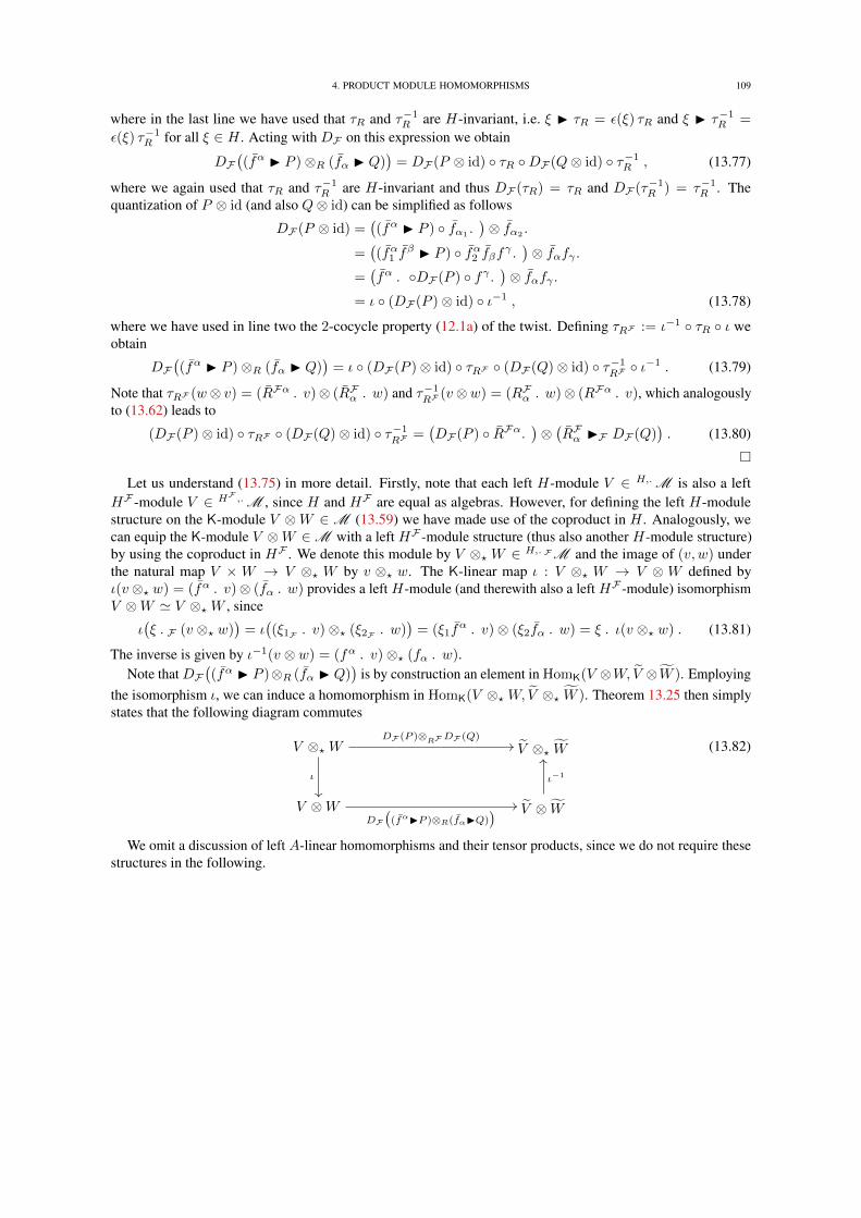
4. PRODUCT MODULE HOMOMORPHISMS 109

where in the last line we have used that τR and τ−1R are H-invariant, i.e. ξ I τR = ε(ξ) τR and ξ I τ−1

R =

ε(ξ) τ−1R for all ξ ∈ H . Acting with DF on this expression we obtain

DF((fα I P )⊗R (fα I Q)

)= DF (P ⊗ id) τR DF (Q⊗ id) τ−1

R , (13.77)

where we again used that τR and τ−1R are H-invariant and thus DF (τR) = τR and DF (τ−1

R ) = τ−1R . The

quantization of P ⊗ id (and also Q⊗ id) can be simplified as follows

DF (P ⊗ id) =((fα I P ) fα1.

)⊗ fα2.

=((fα1 f

β I P ) fα2 fβfγ.)⊗ fαfγ.

=(fα . DF (P ) fγ.

)⊗ fαfγ.

= ι (DF (P )⊗ id) ι−1 , (13.78)

where we have used in line two the 2-cocycle property (12.1a) of the twist. Defining τRF := ι−1 τR ι weobtain

DF((fα I P )⊗R (fα I Q)

)= ι (DF (P )⊗ id) τRF (DF (Q)⊗ id) τ−1

RF ι−1 . (13.79)

Note that τRF (w⊗ v) = (RFα . v)⊗ (RFα . w) and τ−1RF

(v⊗w) = (RFα . w)⊗ (RFα . v), which analogouslyto (13.62) leads to

(DF (P )⊗ id) τRF (DF (Q)⊗ id) τ−1RF

=(DF (P ) RFα.

)⊗(RFα IF DF (Q)

). (13.80)

Let us understand (13.75) in more detail. Firstly, note that each left H-module V ∈ H,.M is also a leftHF -module V ∈ HF ,.M , since H and HF are equal as algebras. However, for defining the left H-modulestructure on the K-module V ⊗W ∈M (13.59) we have made use of the coproduct in H . Analogously, wecan equip the K-module V ⊗W ∈M with a left HF -module structure (thus also another H-module structure)by using the coproduct in HF . We denote this module by V ⊗? W ∈ H,.FM and the image of (v, w) underthe natural map V × W → V ⊗? W by v ⊗? w. The K-linear map ι : V ⊗? W → V ⊗ W defined byι(v ⊗? w) = (fα . v)⊗ (fα . w) provides a left H-module (and therewith also a left HF -module) isomorphismV ⊗W ' V ⊗?W , since

ι(ξ .F (v ⊗? w)

)= ι((ξ1F . v)⊗? (ξ2F . w)

)= (ξ1f

α . v)⊗ (ξ2fα . w) = ξ . ι(v ⊗? w) . (13.81)

The inverse is given by ι−1(v ⊗ w) = (fα . v)⊗? (fα . w).Note that DF

((fα I P )⊗R (fα I Q)

)is by construction an element in HomK(V ⊗W, V ⊗W ). Employing

the isomorphism ι, we can induce a homomorphism in HomK(V ⊗?W, V ⊗? W ). Theorem 13.25 then simplystates that the following diagram commutes

V ⊗?W

ι

DF (P )⊗RFDF (Q)// V ⊗? W

V ⊗WDF

((fαIP )⊗R(fαIQ)

) // V ⊗ W

ι−1

OO(13.82)

We omit a discussion of left A-linear homomorphisms and their tensor products, since we do not require thesestructures in the following.

CHAPTER 14

Bimodule connections

1. Connections on right and left modules

We briefly review the notion of a connection on a right or left module, see e.g. [DV01, Mad00] for anintroduction.

Let A be a unital and associative algebra over K. A differential calculus(Ω•,∧,d

)over A is an N0-graded

algebra(Ω• =

⊕n≥0 Ωn,∧

)over K,1 where Ω0 = A, together with a K-linear map d : Ω• → Ω• of degree one,

satisfying d d = 0 and

d(ω ∧ ω′) = (dω) ∧ ω′ + (−1)deg(ω) ω ∧ (dω′) , (14.1)

for all ω, ω′ ∈ Ω•. The differential d and product ∧ give rise to K-linear maps (denoted by the same symbols)d : Ωn → Ωn+1 and ∧ : Ωn ⊗ Ωm → Ωn+m. Note that in the hypotheses above the K-modules Ωn, n > 0, areA-bimodules, i.e. Ωn ∈ AMA.

Example 14.1. LetM be an N -dimensional smooth manifold and A = C∞(M) be the smooth and complexvalued functions onM. The exterior algebra of differential forms

(Ω• =

⊕n≥0 Ωn,∧

)is an N0-graded algebra

over C, where Ω0 = A and ΩN+n = 0, for all n > 0. The exterior differential d is a differential on(Ω•,∧

),

leading to the differential calculus(Ω•,∧,d

). In this special case Ω• is graded commutative.

Another example is given by the twist deformed differential calculus(Ω•[[λ]],∧?,d

), see Chapter 1. There, the

algebra(Ω•[[λ]],∧?

)is graded quasi-commutative, i.e.

ω ∧? ω′ = (−1)deg(ω) deg(ω′) (Rα . ω′) ∧? (Rα . ω) . (14.2)

Definition 14.2. Let A be a unital and associative algebra over K and(Ω•,∧,d

)be a differential calculus over

A. A connection on a right A-module V ∈ MA is a K-linear map O : V → V ⊗A Ω1, satisfying the rightLeibniz rule, for all v ∈ V and a ∈ A,

O(v · a) = (Ov) · a+ v ⊗A da . (14.3)

Similarly, a connection on a left A-module V ∈ AM is a K-linear map O : V → Ω1 ⊗A V , satisfying the leftLeibniz rule, for all v ∈ V and a ∈ A,

O(a · v) = a · (Ov) + da⊗A v . (14.4)

In case V ∈ AMA is an A-bimodule, we say that a K-linear map O : V → V ⊗A Ω1 is a right connection on V ,if (14.3) is satisfied. Analogously, we say that a K-linear map O : V → Ω1 ⊗A V is a left connection on V , if(14.4) is satisfied.

We denote by ConA(V ) the set of all connections on a right A-module V ∈MA and by ACon(V ) the set ofall connections on a left A-module V ∈ AM . Similarly, we denote by ConA(V ) and ACon(V ) respectively theset of all right and left connections on an A-bimodule V ∈ AMA. Note that given any connection O ∈ ConA(V )and any homomorphism P ∈ HomA(V, V ⊗A Ω1), then O′ = O+ P ∈ ConA(V ) is again a connection, since

O′(v · a) = O(v · a) + P (v · a) = (Ov) · a+ P (v) · a+ v ⊗A da = (O′v) · a+ v ⊗A da . (14.5)

Similarly, let O ∈ ACon(V ) and P ∈ AHom(V,Ω1 ⊗A V ), then O′ = O+ P ∈ ACon(V ), since

O′(a · v) = O(a · v) + P (a · v) = a · (Ov) + a · P (v) + da⊗A v = a · (O′v) + da⊗A v . (14.6)

This means that ConA(V ) and ACon(V ) are affine spaces over the homomorphisms HomA(V, V ⊗A Ω1) orAHom(V,Ω1 ⊗A V ), respectively.

1 In order to stress the analogy to classical differential geometry we denote the product in Ω• by a wedge ∧. However, one has to be abit careful with this notation, since in contrast to the ∧-product in differential geometry our wedge is not necessarily graded commutative.

111

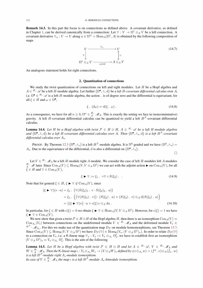
112 14. BIMODULE CONNECTIONS

Remark 14.3. In this part the focus is on connections as defined above. A covariant derivative, as definedin Chapter 1, can be derived canonically from a connection: Let O : V → Ω1 ⊗A V be a left connection. Acovariant derivative Ou : V → V along u ∈ Ω1′ = HomA(Ω1, A) is obtained by the following composition ofmaps

V

O

Ou // V

Ω1 ⊗A V u⊗id// A⊗A V

'

OO(14.7)

An analogous statement holds for right connections.

2. Quantization of connections

We study the twist quantization of connections on left and right modules. Let H be a Hopf algebra andA ∈ H,.A be a left H-module algebra. Let further

(Ω•,∧,d

)be a left H-covariant differential calculus over A,

i.e. Ω• ∈ H,.A is a left H-module algebra, the action . is of degree zero and the differential is equivariant, forall ξ ∈ H and ω ∈ Ω•,

ξ . (dω) = d(ξ . ω) . (14.8)

As a consequence, we have for all n ≥ 0, Ωn ∈ H,.A MA. This is exactly the setting we face in (noncommutative)

gravity. A left H-covariant differential calculus can be quantized to yield a left HF -covariant differentialcalculus.

Lemma 14.4. Let H be a Hopf algebra with twist F ∈ H ⊗ H , A ∈ H,.A be a left H-module algebraand

(Ω•,∧,d

)be a left H-covariant differential calculus over A. Then

(Ω•,∧?,d

)is a left HF -covariant

differential calculus over A?.

PROOF. By Theorem 12.3(Ω•,∧?

)is a left HF -module algebra. It is N0-graded and we have (Ω0,∧?) =

A?. Due to the equivariance of the differential, d is also a differential on(Ω•,∧?

).

Let V ∈ H,.MA be a left H-module right A-module. We consider the case of left H-modules left A-modulesH,.A M later. Since ConA(V ) ⊆ HomK(V, V ⊗A Ω1) we can act with the adjoint action I on ConA(V ), for allξ ∈ H and O ∈ ConA(V ),

ξ I O := ξ1 . O S(ξ2) . . (14.9)

Note that for general ξ ∈ H , ξ I O 6∈ ConA(V ), since

(ξ I O)(v · a) = ξ1 .(O(S(ξ2)1 . v · S(ξ2)2 . a)

)= ξ1 .

((O(S(ξ3) . v)

)· (S(ξ2) . a) + (S(ξ3) . v)⊗A d(S(ξ2) . a)

)=((ξ I O)v

)· a+ ε(ξ) v ⊗A da . (14.10)

In particular, for ξ ∈ H with ε(ξ) = 0 we obtain ξ I O ∈ HomA(V, V ⊗A Ω1). However, for ε(ξ) = 1 we haveξ I O ∈ ConA(V ).

We now show that given a twist F ∈ H⊗H of the Hopf algebraH , then there is an isomorphism ConA(V ) 'ConA?(V?) between connections on the undeformed module V ∈ H,.MA and the deformed module V? ∈HF ,.MA? . For this we make use of the quantization map DF on module homomorphisms, see Theorem 13.7.Since ConA(V ) ⊆ HomK(V, V ⊗A Ω1) we have DF (O) ∈ HomK(V?, (V ⊗A Ω1)?). In order to relate DF (O)to a connection on V?, i.e. a K-linear map O? : V? 7→ V? ⊗A? Ω1

?, we have to establish first an isomorphism(V ⊗A Ω1)? ' V? ⊗A? Ω1

?. This is the aim of the following

Lemma 14.5. Let H be a Hopf algebra with twist F ∈ H ⊗ H and let A ∈ H,.A , V ∈ H,.MA andW ∈ H,.

A MA. Then the K-linear map ι : V?⊗A?W? → (V ⊗AW )? defined by ι(v⊗A?w) = (fα.v)⊗A(fα.w)is a left HF -module right A?-module isomorphism.In case of V ∈ H,.

A MA the map ι is a left HF -module A?-bimodule isomorphism.

2. QUANTIZATION OF CONNECTIONS 113

PROOF. The map ι is well-defined as it is compatible with middle A?-linearity, for all a ∈ A, v ∈ V andw ∈W ,

ι((v ? a)⊗A? w

)=((fα1 f

β . v) · (fα2 fβ . a))⊗A (fα . w)

= (fα . v)⊗A((fα1

fβ . a) · (fα2fβ . w)

)= ι(v ⊗A? (a ? w)

), (14.11)

where in line two we have used (12.4c). Furthermore, ι is a right A?-module homomorphism, for all a ∈ A,v ∈ V and w ∈W ,

ι(v ⊗A? w ? a

)=((fα . v)⊗A (fα1

fβ . w))· (fα2

fβ . a)

= fα .((fβ . v)⊗A (fβ . w)

)· (fα . a) = ι(v ⊗A? w) ? a , (14.12)

and also a left HF -module homomorphism, for all ξ ∈ H , v ∈ V and w ∈W ,

ι(ξ . (v ⊗A? w)

)= ι((ξ1F . v)⊗A? (ξ2F . w)

)= (ξ1f

α . v)⊗A (ξ2fα . w) = ξ . ι(v ⊗A? w) . (14.13)

The inverse ι−1 : (V ⊗AW )? → V? ⊗A? W? is given by ι−1(v ⊗A w) = (fα . v)⊗A? (fα . w).In case of V ∈ H,.

A MA, ι is also a left A?-module homomorphism, for all a ∈ A, v ∈ V and w ∈W ,

ι(a ? v ⊗A? w

)= (fα1 f

β . a) ·((fα2 fβ . v)⊗A (fα . w)

)= (fα . a) · fα .

((fβ . v)⊗A (fβ . w)

)= a ? ι(v ⊗A? w) . (14.14)

We obtain a quantization map DF : ConA(V ) → ConA?(V?) for right module connections by composingDF (O) : V? → (V ⊗A Ω1)? with the isomorphism ι−1 : (V ⊗A Ω1)? → V? ⊗A? Ω1

? according to the followingcommuting diagram

V?

DF (O)((QQQQQQQQQQQQQQ

DF (O)// V? ⊗A? Ω1

?

(V ⊗A Ω1)?

ι−1

OO(14.15)

Theorem 14.6. Let H be a Hopf algebra with twist F ∈ H ⊗ H , A ∈ H,.A be a left H-module algebra,(Ω•,∧,d

)a left H-covariant differential calculus and V ∈ H,.MA a left H-module right A-module. Then the

K-linear map

DF : ConA(V )→ ConA?(V?) , O 7→ DF (O) = ι−1 (DF (O)

)= ι−1 (fα I O) fα. (14.16)

is an isomorphism.

PROOF. The proof follows from a short calculation. Let O ∈ ConA(V ), then for all v ∈ V and a ∈ A,

DF (O)(v ? a) = (fα I O)((fα1 f

β . v) · (fα2 fβ . a))

=((fα I O)(fα1

fβ . v))· (fα2

fβ . a) + ε(fα) (fα1fβ . v)⊗A d(fα2

fβ . a)

=((fα1 f

β I O)(fα2 fβ . v))· (fα . a) + (fβ . v)⊗A d(fβ . a)

= DF (O)(v) ? a+ (fβ . v)⊗A (fβ . da) . (14.17)

In the second line we have used (14.10), in the third line (12.1) and in the last line (14.8) and (14.9). Applyingι−1 we obtain

DF (v ? a) = DF (O)(v) ? a+ v ⊗A? da . (14.18)

DF is invertible via the map O? 7→ D−1F (O?) = ι D−1

F (O?), since for all O ∈ ConA(V ),

D−1F(DF (O)

)= ι

(fα IF (ι−1 DF (O))

) fα. = ι ι−1

(fα IF DF (O)

) fα.

= D−1F(DF (O)

)= O , (14.19)

where for the second equality we have used that ι is a left HF -module isomorphism, thus ξ IF ι−1 = ε(ξ) ι−1,for all ξ ∈ H .

The property D−1F (O?) ∈ ConA(V ), for all O? ∈ ConA?(V?), follows from dequantization of HF and all its

modules via the twist F−1.

114 14. BIMODULE CONNECTIONS

An analogous statement holds true for the quantization of connections on left H-module left A-modules.

Theorem 14.7. Let H be a Hopf algebra with twist F ∈ H ⊗ H , A ∈ H,.A be a left H-module algebra,(Ω•,∧,d

)a left H-covariant differential calculus and V ∈ H,.

A M a left H-module left A-module. Then theK-linear map

DcopF : ACon(V )→ A?Con(V?) , O 7→ Dcop

F (O) = ι−1 (DcopF (O)

)= ι−1 (fα I

cop O) fα.(14.20)

is an isomorphism.

Since the proof is analogous to Theorem 14.6 we can omit it here.

3. Quasi-commutative algebras and bimodules

Let (H,R) be a triangular Hopf algebra and A ∈ H,.A be quasi-commutative. We obtained in Theorem13.19 that the map DR, i.e. the quantization isomorphism with F = R, provides an isomorphism of right and leftmodule homomorphisms between quasi-commutative bimodules. The aim of this section is to prove a similarstatement for right and left connections on a quasi-commutative bimodule V ∈ H,.

A MA.

Theorem 14.8. Let (H,R) be a triangular Hopf algebra and A ∈ H,.A , V ∈ H,.A MA be quasi-commutative.

Let further(Ω•,∧,d

)be a graded quasi-commutative left H-covariant differential calculus over A. Then the

K-linear map

DR : ConA(V )→ ACon(V ) , O 7→ DR(O) = τR (DR(O)

)(14.21)

is an isomorphism, where DR is the quantization isomorphism with F = R and τR : V ⊗A Ω1 7→ Ω1 ⊗A V isthe R-flip map, i.e. τR(v ⊗A ω) = (Rα . ω)⊗A (Rα . v).

PROOF. By Lemma 13.18 we have A? = Aop, Ω? = Ωop and V? = V op. Using this and Theorem 14.6 weobtain, for all O ∈ ConA(V ), a ∈ A and v ∈ V ,

DR(O)(a · v) = DR(O)(v ? a) = DR(O)(v) ? a+ (Rα . v)⊗A d(Rα . a)

= a ·DR(O)(v) + (Rα . v)⊗A (Rα . da) . (14.22)

Applying the bimodule isomorphism τR and using triangularity R21 = R−1 we find

DR(O)(a · v) = a · DR(O)(v) + da⊗A v . (14.23)

Thus, DR(O) ∈ ACon(V ). The map DR is invertible via

D−1R : ACon(V )→ ConA(V ) , O 7→ D−1

R (O) = τR (D−1R (O)

), (14.24)

where D−1R (O) = Dcop

R (O) = (Rα Icop O) Rα.. (Note that τR = τ−1R since H is triangular.)

4. Extension to product modules

Motivated by the studies on product module homomorphisms in Chapter 13, Section 4, we now investigate theextension of connections to product modules. This is of major importance for noncommutative gravity, since itprovides a construction principle for connections on deformed tensor fields in terms of a fundamental connectionson the deformed vector fields or one-forms. For the construction presented below it is essential to assume atriangular Hopf algebra and quasi-commutative algebras and modules.

Theorem 14.9. Let (H,R) be a triangular Hopf algebra and A ∈ H,.A , W ∈ H,.A MA be quasi-commutative.

Let further(Ω•,∧,d

)be a graded quasi-commutative left H-covariant differential calculus over A and V ∈

H,.MA, OV ∈ ConA(V ) and OW ∈ ConA(W ). Then the K-linear map OV ⊕R OW : V ⊗A W → V ⊗AW ⊗A Ω1 defined by

OV ⊕R OW := τR 23 (OV ⊗R id) + id⊗R OW (14.25)

is a connection on V ⊗AW ∈ H,.MA. Here τR 23 = id⊗ τR is the R-flip map acting on the second and thirdleg of the tensor product and the R-tensor product of K-linear maps was defined in (13.61).

4. EXTENSION TO PRODUCT MODULES 115

PROOF. Firstly, note that OV ⊗R id = OV ⊗ id, since id is H-invariant. We have to show that (14.25)satisfies the right Leibniz rule (14.3) and that it is compatible with A-middle linearity on V ⊗A W . For theproof we denote both connections OV and OW by O in order to simplify the notation. We start with the formerproperty, for all v ∈ V , w ∈W and a ∈ A,

(O⊕R O)(v ⊗A w · a) = τR 23

((Ov)⊗A w · a

)+ (Rα . v)⊗A (Rα I O)(w · a)

= (O⊕R O)(v ⊗A w) · a+ ε(Rα) (Rα . v)⊗A w ⊗A da

= (O⊕R O)(v ⊗A w) · a+ v ⊗A w ⊗A da , (14.26)

where in the second line we have used that τR is a bimodule isomorphism and (14.10), and in the last line thenormalization property of the R-matrix (13.38a)

We now prove compatibility of (14.25) with A-middle linearity, for all v ∈ V , w ∈W and a ∈ A,

(O⊕R O)(v · a⊗A w) = τR 23

(O(v · a)⊗A w

)+ (Rα . (v · a))⊗A (Rα I O)(w)

= τR 23

((Ov)⊗A a · w + v ⊗A da⊗A w

)+ (Rα . v)⊗A (Rβ . a) · (RβRα I O)(w)

= τR 23

((Ov)⊗A a · w

)+ (Rα . v)⊗A (Rα I O)(a · w)

= (O⊕R O)(v ⊗A a · w) , (14.27)

where in the second line we have used the right Leibniz rule (14.3) and the property (13.36) of the R-matrix. Thethird line follows by using quasi-commutativity, triangularity, the properties (13.36) and (13.38) of the R-matrixand (14.10). (Hint: It is easier to show that line two follows from line three.)

The Hopf algebra H acts on the connection OV ⊕R OW via the adjoint action I. We obtain for all ξ ∈ H

ξ I (OV ⊕R OW ) = ξ I(τR 23 (OV ⊗R id) + id⊗R OW

)= τR 23

((ξ I OV )⊗R id

)+ id⊗R (ξ I OW )

= (ξ I OV )⊕R (ξ I OW ) , (14.28)

where we have used that τR and id are invariant under H and (13.64a).The sum ⊕R of connections canonically extends to arbitrary tensor products and is compatible with the

bimodule isomorphism τR due to the following

Theorem 14.10. Let (H,R) be a triangular Hopf algebra and A ∈ H,.A , W,Z ∈ H,.A MA be quasi-

commutative. Let further(Ω•,∧,d

)be a graded quasi-commutative left H-covariant differential calculus

over A and V ∈ H,.MA, OV ∈ ConA(V ), OW ∈ ConA(W ) and OZ ∈ ConA(Z). Then(OV ⊕R OW

)⊕R OZ = OV ⊕R

(OW ⊕R OZ

)(14.29)

and

OZ ⊕R OW = τR 12 (OW ⊕R OZ

) τR , (14.30)

where τR 12 = τR ⊗ id is the R-flip map acting on the first and second leg of the tensor product.

PROOF. We denote by τR i i+1 = id⊗ · · · ⊗ τR ⊗ · · · ⊗ id the R-flip map acting on the i-th and (i+ 1)-thleg of a tensor product. The R-flip map exchanging the i-th leg with the (i+1)-th and (i+2)-th leg is denoted byτR i (i+1 i+2) and similarly τR (i i+1) i+2 is theR-flip map exchanging the i-th and (i+1)-th leg with the (i+2)-thleg. For example, τR (12)3(a⊗b⊗c) = (Rα .c)⊗ Rα . (a⊗b) and τR 1(23)(a⊗b⊗c) = Rα . (b⊗c)⊗ (Rα .a).Let us first show the associativity property (14.29). To simplify notation we denote all connections by O.

(O⊕R O)⊕R O = τR 34 ((O⊕R O)⊗R id

)+ id⊗R id⊗R O

= τR 34 (τR 23 (O⊗R id⊗R id) + id⊗R O⊗R id

)+ id⊗R id⊗R O

= τR 34 τR 23 (O⊗R id⊗R id) + τR 34 (id⊗R O⊗R id) + id⊗R id⊗R O= τR 2(34) (O⊗R id⊗R id) + id⊗R

(τR 23 (O⊗R id) + id⊗R O

)= τR 2(34) (O⊗R id⊗R id) + id⊗R (O⊕R O)

= O⊕R (O⊕R O) . (14.31)

We have frequently used (13.64c) together with the fact that id and τR are H-invariant. In line four we have alsoused τR 2(34) = τR 34 τR 23, which follows from the properties of the R-matrix (13.36).

116 14. BIMODULE CONNECTIONS

We now show the property (14.30). The strategy is to express all R-tensor products by usual ones using(13.62). Note that τ−1

R = τR for a triangular Hopf algebra.

OZ ⊕R OW = τR 23 (OZ ⊗ id) + id⊗R OW= τR 23 (OZ ⊗ id) + τR (12)3 (OW ⊗ id) τR= τR 23 (OZ ⊗ id) + τR 12 τR 23 (OW ⊗ id) τR= τR 12

(τR 12 τR 23 (OZ ⊗ id) τR + τR 23 (OW ⊗ id)

) τR

= τR 12 (OW ⊕R OZ) τR . (14.32)

In line three we have used τR (12)3 = τR 12 τR 23, which follows from the properties of the R-matrix (13.36).

It remains to study the quantization of the sum of two connections (14.25). By construction,DF (OV ⊕ROW ) :(V ⊗AW )? → (V ⊗AW ⊗A Ω1)? is a K-linear map. Analogously to Lemma 14.5 there is a left HF -moduleright A?-module isomorphism ι123 : V? ⊗A? W? ⊗A? Ω1

? → (V ⊗A W ⊗A Ω1)? given by the followingcommuting diagram2

V? ⊗A? W? ⊗A? Ω1?

ι123++VVVVVVVVVVVVVVVVVV

ι23

ι12 // (V ⊗AW )? ⊗A? Ω1?

ι(12)3

V? ⊗A? (W ⊗A Ω1)? ι1(23)

// (V ⊗AW ⊗A Ω1)?

(14.33)

Theorem 14.11. Let (H,R) be a triangular Hopf algebra with twist F ∈ H ⊗H and A ∈ H,.A , W ∈ H,.A MA

be quasi-commutative. Let further(Ω•,∧,d

)be a graded quasi-commutative left H-covariant differential

calculus and V ∈ H,.MA, OV ∈ ConA(V ) and OW ∈ ConA(W ). Then the following diagram commutes

V? ⊗A? W?

DF (OV )⊕RF DF (OW )//

ι

V? ⊗A? W? ⊗A? Ω1?

(V ⊗AW )?DF (OV ⊕ROW )

// (V ⊗AW ⊗A Ω1)?

ι−1123

OO(14.34)

PROOF. To simplify notation we denote all connections by O. Using K-linearity of DF and that τR and idare invariant under H , we obtain

DF (O⊕R O) = DF(τR 23 (O⊗R id) + id⊗R O

)= τR 23 DF (O⊗R id) +DF (id⊗R O) . (14.35)

Theorem 13.25 and H-invariance of id implies

DF (O⊕R O) = τR 23 ι(12)3 (DF (O)⊗RF id

) ι−1 + ι1(23)

(id⊗RF DF (O)

) ι−1

= τR 23 ι(12)3 ι12 (DF (O)⊗RF id

) ι−1 + ι1(23) ι23

(id⊗RF DF (O)

) ι−1 ,

(14.36)

where in the last line we have also used (13.64c) and that ι and id are H-invariant.We now compose this with ι from the right and with ι−1

123 from the left. Using the diagram (14.33), τR 23 ι1(23) = ι1(23) τR 23 and τRF 23 = ι−1

23 τR 23 ι23, we find

ι−1123 DF (O⊕R O) ι = τRF 23

(DF (O)⊗RF id

)+(id⊗RF DF (O)

)= DF (O)⊕RF DF (O) . (14.37)

5. Extension to the dual module

It remains to provide an extension of connections O ∈ ConA(V ) to the dual module V ′ = HomA(V,A). Thisconstruction is of major importance in noncommutative gravity, since given a connection on e.g. vector fields Ξ,we have to know how to obtain from it a connection on one-forms Ω1, the dual of Ξ. We focus only on rightconnections ConA(V ) and the right dual V ′ = HomA(V,A) of a module V , since left connections and left dualsfollow from a mirror construction as above.

2 The indices on ι label the legs it acts on.

5. EXTENSION TO THE DUAL MODULE 117

For the discussion we have to assume that the module V is finitely generated and projective, a propertywhich is also required in every other approach to connections on modules known to us, see e.g. [DV01, Mad00].For describing noncommutative vector bundles this restriction is motivated by the Serre-Swan theorem [Ser55,Swa62], stating that vector bundles over commutative, smooth and compact manifolds are equivalent to finitelygenerated and projective modules over the algebra of smooth functions. Before defining and discussing finitelygenerated and projective modules in detail, let us briefly explain why this property is essential for describingdual connections. Using a connection O ∈ ConA(V ) and the differential d on A, we can induce a K-linear mapV ′ → HomA(V,Ω1) by v′ 7→ d v′ −∧ (v′ ⊗ id) O. For a finitely generated and projective module V thereis an isomorphism HomA(V,Ω1) ' Ω1 ⊗A V ′. Composing the induced map V ′ → HomA(V,Ω1) with thisisomorphism we obtain a K-linear map V ′ → Ω1 ⊗A V ′. We are going to prove in detail that this map is a leftconnection on V ′. Using Theorem 14.8 we can induce from this left connection a right connection on V ′ in thequasi-commutative setting.

There are various equivalent definitions of a finitely generated and projective module over a ring, see e.g. thebook [Lam99]. We do not have to go into the details and use the very convenient characterization of this type ofmodule in terms of a pair of dual bases.

Lemma 14.12 (Dual Basis Lemma). LetA ∈ A be a unital and associative algebra. A rightA-module V ∈MA

is finitely generated and projective, if and only if there exists a family of elements vi ∈ V : i = 1, . . . , n andA-linear functionals v′i ∈ V ′ = HomA(V,A) : i = 1, . . . , n with n ∈ N, such that for any v ∈ V we have

v =

n∑i=1

vi · v′i(v) . (14.38)

Analogously, a left A-module V ∈ AM is finitely generated and projective, if and only if there exists a familyof elements vi ∈ V : i = 1, . . . , n and A-linear functionals v′i ∈ ′V = AHom(V,A) : i = 1, . . . , n withn ∈ N, such that for any v ∈ V we have

v =

n∑i=1

v′i(v) · vi . (14.39)

A proof of this lemma can be found e.g. in [Lam99]. The set vi, v′i : i = 1, . . . , n is loosely referred to “pairof dual bases” for V , even though vi is just a generating set of V and not a basis.

Finitely generated and projective modules enjoy the following important properties.

Proposition 14.13. Let V ∈MA be a finitely generated and projective right A-module with a pair of dual basesvi, v′i : i = 1, . . . , n. For any v ∈ V let v′′ ∈ V ′′ := AHom(V ′, A) be defined by v′′(v′) := v′(v), for allv′ ∈ V ′. We have

(1) v′i, v′′i : i = 1, . . . , n is a pair of dual bases for V ′

(2) V ′ is a finitely generated and projective left A-module(3) The natural map V → V ′′ , v 7→ v′′ is an isomorphism of right A-modules

PROOF. Proof of (1):We have to show that v′ =

∑ni=1 v

′′i (v′) · v′i, for all v′ ∈ V ′. Evaluating the right hand side on an arbitrary v ∈ V

we obtainn∑i=1

v′′i (v′) v′i(v) =

n∑i=1

v′(vi) v′i(v) = v′

(n∑i=1

vi · v′i(v)

)= v′(v) . (14.40)

Proof of (2):Follows directly from the dual basis lemma.Proof of (3):The map V → V ′′ , v 7→ v′′ is injective, since let 0 = v′′ we have v′′(v′) = v′(v) = 0, for all v′ ∈ V ′, and thusby the dual basis lemma v =

∑ni=1 vi · v′i(v) = 0. It is also surjective, since v′′i is a generating set of V ′′.

We now come to the property of finitely generated and projective modules which is most relevant for ourstudies.

Proposition 14.14. Let V ∈MA be a finitely generated and projective right A-module and let W ∈MA. Thenthere exists an isomorphism ϕ : W ⊗A V ′ → HomA(V,W ).If in addition V,W ∈ AMA are A-bimodules, then ϕ is an isomorphism between the A-bimodules W ⊗A V ′ ∈AMA and HomA(V,W ) ∈ AMA.

118 14. BIMODULE CONNECTIONS

For left H-module A-bimodules V,W ∈ H,.A MA, ϕ is an isomorphism between the left H-module A-bimodules

W ⊗A V ′ ∈ H,.A MA and HomA(V,W ) ∈ H,I

A MA.

PROOF. We define a K-linear map ϕ : W ⊗A V ′ → HomA(V,W ) by, for all v ∈ V ,(ϕ(w ⊗A v′)

)(v) :=

w · v′(v). Employing the pair of dual bases this map is invertible via

ϕ−1 : HomA(V,W )→W ⊗A V ′ , P 7→ ϕ−1(P ) =

n∑i=1

P (vi)⊗A v′i . (14.41)

Indeed, we obtain for all v ∈ V and P ∈ HomA(V,W ),(ϕ(ϕ−1(P ))

)(v) =

n∑i=1

(ϕ(P (vi)⊗A v′i)

)(v) =

n∑i=1

P (vi) · v′i(v)

= P

(n∑i=1

vi · v′i(v)

)= P (v) , (14.42)

and for all w ∈W and v′ ∈ V ′

ϕ−1(ϕ(w ⊗A v′)

)=

n∑i=1

w · v′(vi)⊗A v′i = w ⊗An∑i=1

v′′i (v′) · v′i = w ⊗A v′ . (14.43)

Let now V,W ∈ AMA be A-bimodules, then V ′,W ⊗A V ′ and HomA(V,W ) are also A-bimodules. Theisomorphism ϕ respects the bimodule structure, since for all a, b ∈ A, w ∈W , v′ ∈ V ′ and v ∈ V ,(

ϕ(a · w ⊗A v′ · b))(v) = a · w · v′(b · v) = a ·

(ϕ(w ⊗A v′)

)(b · v)

=(a · ϕ(w ⊗A v′) · b

)(v) . (14.44)

Let V,W ∈ H,.A MA be left H-module A-bimodules, then V ′,W ⊗A V ′ and HomA(V,W ) are also left

H-module A-bimodules. The isomorphism ϕ respects the left H-module structure, since for all ξ ∈ H , w ∈W ,v′ ∈ V ′ and v ∈ V ,(

ϕ(ξ . (w ⊗A v′)))(v) = (ξ1 . w) · (ξ2 I v′)(v) = (ξ1 . w) ·

(ξ2 . v

′(S(ξ3) . v))

= ξ1 .(w · v′(S(ξ2) . v)

)=(ξ I

(ϕ(w ⊗A v′)

))(v) . (14.45)

This property of finitely generated and projective modules now allows us to induce a connection on thedual module V ′ = HomA(V,A), see also [DV01, Mad00] for similar discussions. Let A ∈ A be a unitaland associative algebra and let

(Ω•,∧,d

)be a differential calculus over A. Let further V ∈MA be a finitely

generated and projective right A-module. Given a connection O ∈ ConA(V ) we define the following K-linearmap

OHom : V ′ → HomA(V,Ω1) , v′ 7→ OHom(v′) = d v′ − ∧ (v′ ⊗ id) O . (14.46)

In the second term we have canonically extended v′ ∈ HomA(V,A) to a right A-linear map v′ ⊗ id : V ⊗AΩ1 → A ⊗A Ω1 by (v′ ⊗ id)(v ⊗A ω) := v′(v) ⊗A ω. The map ∧ : A ⊗A Ω1 → Ω1 is the A-bimodulehomomorphism associated to the product in Ω•, i.e. ∧(a ⊗A ω) = a ∧ ω = a · ω. The right A-linearity ofOHom(v′) ∈ HomA(V,Ω1) is easily shown, for all a ∈ A, v′ ∈ V ′ and v ∈ V ,(

OHom(v′))

(v · a) = d(v′(v · a)

)− ∧

((v′ ⊗ id)

(O(v · a)

))= d(v′(v)) · a+ v′(v) · da− ∧

((v′ ⊗ id)

(Ov))· a− ∧

((v′ ⊗ id)(v ⊗A da)

)=(OHom(v′)

)(v) · a . (14.47)

Employing the left A-module isomorphism ϕ−1 : HomA(V,Ω1) → Ω1 ⊗A V ′ (14.41) we can induce aK-linear map O′ : V ′ → Ω1 ⊗A V ′ via the following diagram

V ′OHom

//

O′((QQQQQQQQQQQQQQQ HomA(V,Ω1)

ϕ−1

Ω1 ⊗A V ′

(14.48)

5. EXTENSION TO THE DUAL MODULE 119

The map O′ acting on v′ ∈ V ′ reads explicitly

O′(v′) = ϕ−1(OHom(v′)

)=

n∑i=1

(d(v′(vi))− ∧

((v′ ⊗ id)(Ovi)

))⊗A v′i . (14.49)

We can now show that O′ is a connection on V ′, see also [DV01, Mad00].

Theorem 14.15. In the hypotheses above, the map O′ (14.48) is a connection on the left A-module V ′ ∈ AM .

PROOF. Using (14.49) we have for all a ∈ A and v′ ∈ V ′

O′(a · v′) =

n∑i=1

(d(a v′(vi))− a · ∧

((v′ ⊗ id)(Ovi)

))⊗A v′i

=

n∑i=1

(da · v′(vi) + a · d(v′(vi))− a · ∧

((v′ ⊗ id)(Ovi)

))⊗A v′i

= da⊗An∑i=1

v′′i (v′) · v′i + a · O′(v′)

= da⊗A v′ + a · O′(v′) . (14.50)

This well-known theorem serves as a basis for discussing the twist quantization of dual connections. For thiswe require the following technical

Lemma 14.16. Let H be a Hopf algebra with twist F ∈ H ⊗ H , A ∈ H,.A and V,W ∈ H,.MA. Letfurther V be finitely generated and projective. We denote by ϕ : W ⊗A V ′ → HomA(V,W ) the left H-moduleisomorphism of Proposition 14.14 and by ϕ? : W? ⊗A? (V?)

′ → HomA?(V?,W?) the K-linear map defined by,for all v ∈ V?,

(ϕ?(w ⊗A? v′?)

)(v) := w ? v′?(v). Then the following diagram commutes

W? ⊗A? (V?)′ ϕ? //

id⊗D−1F

HomA?(V?,W?)

D−1F

W? ⊗A? (V ′)?

ι

(W ⊗A V ′)? ϕ// (HomA(V,W ))?

(14.51)

PROOF. Using the explicit expression for D−1F (12.30), we find when going the upper path, for all v ∈ V?,(

D−1F(ϕ?(w ⊗A? v′?)

))(v) = fα .

(w ? v′?

(χS(fα) . v

))= (fα1 f

β . w) · fα2 fβ . v′?(χS(fα) . v

)= (fα . w) · fα1

fβ . v′?(χS(fβ)S(fα2

) . v)

= (fα . w) ·(fα I D

−1F (v′?)

)(v) , (14.52)

where in line three we have used the cocycle condition (12.4c). Following the lower path we find, for all v ∈ V?,(ϕ(ι(w ⊗A? D−1

F (v′?))))

(v) =(ϕ(

(fα . w)⊗A(fα I D

−1F (v′?)

)))(v)

= (fα . w) ·(fα I D

−1F (v′?)

)(v) . (14.53)

We now prove that quantizing the dual connection is equivalent to dualizing the quantized connection.

Theorem 14.17. Let H be a Hopf algebra with twist F ∈ H ⊗H , A ∈ H,.A and V ∈ H,.MA. Let further(Ω•,∧,d

)be a left H-covariant differential calculus and let V be finitely generated and projective. Then the

120 14. BIMODULE CONNECTIONS

following diagram commutes

ConA(V )′

//

DF

ACon(V ′)

DcopF

ConA?(V?) ′//A?Con((V?)

′) ' A?Con((V ′)?)

(14.54)

PROOF. Let O ∈ ConA(V ) be a connection on V . Following the upper path in the diagram, we firstconstruct its dualO′ ∈ ACon(V ′) and then apply the quantization map Dcop

F yielding the connection DcopF (O′) ∈

A?Con((V ′)?). In particular, DcopF (O′) is a map (V ′)? → Ω1

? ⊗A? (V ′)?. Using that ϕ is a left H-moduleisomorphism, we have

DcopF (O′) = ι−1 Dcop

F (ϕ−1 OHom) = ι−1 ϕ−1 DcopF (OHom) . (14.55)

When acting on an element v′ ∈ (V ′)? we get(DcopF (O′)

)(v′) = ι−1

(ϕ−1

(d ? v′ − ∧ ? (v′ ⊗ id) ? O

)). (14.56)

Going the lower path, we first quantize the connection O yielding the connection DF (O) ∈ ConA?(V?) andthen construct its dual

(DF (O)

)′ ∈ A?Con((V?)′). In particular,

(DF (O)

)′is a map (V?)

′ → Ω1? ⊗A? (V?)

′,which reads when acting on v′? ∈ (V?)

′(DF (O)

)′(v′?) = ϕ−1

?

(d v′? − ∧? (v′? ⊗ id) DF (O)

). (14.57)

Since (V ′)? ' (V?)′ via the map DF , equality of the connections Dcop

F (O′) and(DF (O)

)′means that the

following diagram has to commute

(V ′)?DcopF (O′)

//

DF

Ω1? ⊗A? (V ′)?

id⊗DF

(V?)′ (

DF (O))′ // Ω1

? ⊗A? (V?)′

(14.58)

Going the upper path, using (14.56) and acting with ϕ? = DF ϕ ι (id⊗D−1F ) (see (14.51)) on the result,

we obtain

ϕ?

((id⊗DF )

(DcopF (O′)(v′)

))= DF

(d ? v′ − ∧ ? (v′ ⊗ id) ? O

)= d DF (v′)− ∧? ι−1 DF

(v′ ⊗ id

) ι DF (O) , (14.59)

where we have used that d and ∧ are H-invariant and ∧? = ∧ ι. Going the lower path, using (14.57) and actingalso with ϕ? on the result, we obtain

ϕ?

((DF (O)

)′(DF (v′))

)= d DF (v′)− ∧? (DF (v′)⊗ id) DF (O) . (14.60)

These two expressions are equal, since (DF (v′)⊗ id) = ι−1 DF(v′ ⊗ id

) ι due to Theorem 13.25.

In the quasi-commutative setting, i.e. assuming (H,R) to be a triangular Hopf algebra, and A ∈ H,.A ,(Ω•,∧,d) and V ∈ H,.

A MA to be (graded) quasi-commutative, we can derive a right connection on V ′ byemploying Theorem 14.8. The right connections O ∈ ConA(V ) and D−1

R (O′) ∈ ConA(V ′) then can beextended to arbitrary tensor products of V and V ′ as shown in Theorem 14.10. In the case of (noncommutative)gravity, this provides us with a prescription to construct a connection on arbitrary tensor fields.

CHAPTER 15

Curvature and torsion

The aim of this chapter is to introduce curvature and torsion into the framework developed above. This is anessential step towards noncommutative gravity, see Chapter 16, and also noncommutative Yang-Mills theory. Foran introduction to connections, curvature and torsion, see [DV01, Mad00].

Let A ∈ A be a unital and associative algebra, (Ω•,∧,d) be a differential calculus over A and V ∈MA aright A-module. We can extend any connection O ∈ ConA(V ) to a K-linear map O : V ⊗A Ω1 → V ⊗A Ω2 bydefining

O := (id⊗ ∧) (O⊗ id) + (id⊗ d) , (15.1)

where the A-bimodule homomorphism ∧ : Ω1 ⊗A Ω1 → Ω2 is given by the product in Ω•. The map O iswell-defined, since it is compatible with middle A-linearity, for all v ∈ V , ω ∈ Ω1 and a ∈ A,

O(v · a⊗A ω

)= (id⊗ ∧)

((Ov) · a⊗A ω + v ⊗A da⊗A ω

)+ v · a⊗A dω

= (id⊗ ∧)((Ov)⊗A a · ω

)+ v ⊗A

(da ∧ ω + a · dω

)= O

(v ⊗A a · ω

). (15.2)

Definition 15.1. The curvature of a connection O ∈ ConA(V ) is defined by the right A-linear map

R := O O : V → V ⊗A Ω2 . (15.3)

We show that R is right A-linear. First, note that for all v ∈ V , ω ∈ Ω1 and a ∈ A,

O(v ⊗A ω · a

)= (id⊗ ∧)

((Ov)⊗A ω · a

)+ v ⊗A d(ω · a)

= (id⊗ ∧)((Ov)⊗A ω

)· a+ v ⊗A

((dω) · a− ω ∧ da

)= O

(v ⊗A ω

)· a− (id⊗ ∧)

(v ⊗A ω ⊗A da

). (15.4)

Using this we obtain, for all v ∈ V and a ∈ A,

R(v · a) = O(O(v · a)

)= O

((Ov) · a+ v ⊗A da

)= O

(Ov)· a− (id⊗ ∧)

((Ov)⊗A da

)+ (id⊗ ∧)

((Ov)⊗A da

)+ v ⊗A dda

= R(v) · a . (15.5)

Remark 15.2. In classical pseudo-Riemannian geometry the usual definition of curvature is as a map Riem :Ξ⊗AΞ⊗AΞ→ Ξ, see also Chapter 1, which is antisymmetric in the first two legs. This map can be equivalentlydescribed by a tensor in Ξ⊗A Ω1 ⊗A Ω2, the Riemann tensor, which, due to duality of Ξ and Ω1, canonicallygives rise to a map Ω1 → Ω1 ⊗A Ω2. In classical pseudo-Riemannian geometry this map coincides with thecurvature defined above. For our purpose it is more convenient to work with the Definition 15.1.

We now study the behavior of the curvature R under twist quantization. For this let H be a Hopf algebrawith twist F ∈ H ⊗ H and let A ∈ H,.A , V ∈ H,.MA and

(Ω•,∧,d

)be a left H-covariant differential

calculus over A. Twist quantization yields the deformed Hopf algebra HF , the left HF -modules A? ∈ HF ,.A ,V? ∈ HF ,.MA? and the left HF -covariant differential calculus

(Ω•,∧?,d

), see Theorems 12.2, 12.3, 12.4 and

Lemma 14.4. Let O? ∈ ConA?(V?) be any connection on deformed module V?, then its curvature is given by theright A?-linear map R? : V? → V? ⊗A? Ω2

?

R? = O? O? = (id⊗ ∧?) (O? ⊗ id) O? + (id⊗ d) O? . (15.6)

Due to Theorem 14.6 there is a unique connection O ∈ ConA(V ), such that O? = DF (O) = ι−1 DF (O). Wefind the following expression for the curvature R? in terms of the undeformed connection O.

Proposition 15.3. In the hypotheses above, the curvature R? of any connection O? ∈ ConA?(V?) can beexpressed in terms of the corresponding undeformed connection O ∈ ConA(V ) by

R? = ι−1 DF(

(id⊗ ∧) ? (O⊗ id) ? O+ (id⊗ d) ? O), (15.7)

121

122 15. CURVATURE AND TORSION

where the ?-composition was defined in (12.38) and ι−1 in Lemma 14.5.

PROOF. We investigate the individual terms in (15.6) and make use of Theorem 13.25.Firstly, the following diagram commutes

V? ⊗A? Ω1? ⊗A? Ω1

?

id⊗∧? //

ι123

V? ⊗A? Ω2?

(V ⊗A Ω1 ⊗A Ω1)?DF (id⊗∧)

// (V ⊗A Ω2)?

ι−1

OO(15.8)

Here it is essential to note that ∧ is a left H-module homomorphism, i.e. ξ I ∧ = ε(ξ)∧ for all ξ ∈ H .For the second term, O? ⊗ id, we find the following commuting diagram

V? ⊗A? Ω1?

O?⊗id//

ι

V? ⊗A? Ω1? ⊗A? Ω1

?

(V ⊗A Ω1)?DF (O⊗id)

// (V ⊗A Ω1 ⊗A Ω1)?

ι−1123

OO(15.9)

Since the differential d is equivariant, we obtain the commuting diagram

V? ⊗A? Ω1?

id⊗d//

ι

V? ⊗A? Ω2?

(V ⊗A Ω1)?DF (id⊗d)

// (V ⊗A Ω2)?

ι−1

OO(15.10)

Combining these results, we can express the curvature R? in terms of O by (15.7).

In (noncommutative) gravity a module V of particular interest is the module of one-forms Ω1. A rightconnection O ∈ ConA(Ω1) is also called a linear connection. Choosing V = Ω1 allows us to define andstudy torsion and the Ricci curvature, a particular contraction of the curvature R above. Since these objects areimportant for noncommutative gravity we are now going to investigate their properties and behavior under twistquantization.

Let A ∈ A be a unital and associative algebra and (Ω•,∧,d) be a differential calculus over A.

Definition 15.4. The torsion of a linear connection O ∈ ConA(Ω1) is defined by the right A-linear map

T : Ω1 → Ω2 , ω 7→ T(ω) = ∧(Oω)

+ dω . (15.11)

We now show that T is right A-linear, for all ω ∈ Ω1 and a ∈ A,

T(ω · a) = ∧((Oω) · a+ ω ⊗A da

)+ d(ω · a)

= ∧((Oω)

)· a+ ω ∧ da+ (dω) · a− ω ∧ da

= T(ω) · a . (15.12)

Remark 15.5. In classical pseudo-Riemannian geometry the usual definition of torsion is as a map Tor :Ξ⊗A Ξ→ Ξ, see also Chapter 1, which is antisymmetric. This map can be equivalently described by a tensor inΞ⊗A Ω2, the torsion tensor, which, due to duality of Ξ and Ω1, canonically gives rise to a map Ω1 → Ω2. Inclassical pseudo-Riemannian geometry this map coincides with the torsion defined above.

We now study the behavior of the torsion T under twist quantization. For this let H be a Hopf algebrawith twist F ∈ H ⊗H , A ∈ H,.A and let

(Ω•,∧,d

)be a left H-covariant differential calculus over A. Let

O? ∈ ConA?(Ω1?) be any linear connection on deformed module Ω1

?, then its torsion is given by the rightA?-linear map T? : Ω1

? → Ω2?

T? = ∧? O? + d . (15.13)

Due to Theorem 14.6 there is a unique linear connectionO ∈ ConA(Ω1), such thatO? = DF (O) = ι−1DF (O).We find the following expression for the torsion T? in terms of the undeformed linear connection O.

15. CURVATURE AND TORSION 123

Proposition 15.6. In the hypotheses above, the torsion T? of any linear connection O? ∈ ConA?(Ω1?) can be

expressed in terms of the corresponding undeformed linear connection O ∈ ConA(Ω1) by

T? = DF (T) . (15.14)

PROOF. Using ∧? = ∧ ι and O? = ι−1 DF (O) we obtain for (15.13)

T? = ∧ DF (O) + d = DF (T) , (15.15)

where in the second equality we have used that ξ I ∧ = ε(ξ)∧ and ξ I d = ε(ξ) d, for all ξ ∈ H .

These results on the curvature and torsion hold in a very general setting. In particular, we did not haveto assume the Hopf algebra to be (quasi)triangular and the modules to be finitely generated and projective orquasi-commutative. However, for constructing the Ricci curvature as a contraction of the curvature R we have toadd some additional assumptions. In the following, let (H,R) be a triangular Hopf algebra and let A ∈ H,.A bequasi-commutative. Let further

(Ω•,∧,d

)be a graded quasi-commutative left H-covariant differential calculus

over A and Ω1 ∈ H,.A MA be finitely generated and projective as a right A-module. Moreover, we assume that

there is an injective left H-module A-bimodule homomorphism Ω2 → Ω1 ⊗A Ω1.1

In order to construct the Ricci curvature we first have to define a contraction map. In the hypotheses above, letV ∈ H,.

A MA be quasi-commutative, and finitely generated and projective as a right A-module. We define thecontraction map contr : V ⊗A V ′ → A by the following diagram

V ⊗A V ′

τR))RRRRRRRRRRRRR

contr // A

V ′ ⊗A V

ev

OO(15.16)

where ev : V ′ ⊗A V → A is the evaluation map defined by ev(v′ ⊗A v) = v′(v). Note that ev is a leftH-module A-bimodule homomorphism, and hence contr is also a left H-module A-bimodule homomorphismas a composition of maps with this property.

Due to the assumed injective left H-module A-bimodule homomorphism Ω2 → Ω1 ⊗A Ω1, we can regard thecurvature as a right A-linear map Ω1 → Ω1 ⊗A Ω1 ⊗A Ω1, simply by composing R with this homomorphism.Applying also the map ϕ−1 : HomA(Ω1,Ω1 ⊗A Ω1 ⊗A Ω1)→ Ω1 ⊗A Ω1 ⊗A Ω1 ⊗A Ω1′ of Proposition 14.14,we obtain from the curvature R the curvature tensor R ∈ Ω1 ⊗A Ω1 ⊗A Ω1 ⊗A Ω1′.

Definition 15.7. In the hypotheses above, the Ricci curvature of a linear connection O ∈ ConA(Ω1) is definedby the application of the following contraction on the curvature tensor

Ω1 ⊗A Ω1 ⊗A Ω1 ⊗A Ω1′ id⊗id⊗contr// Ω1 ⊗A Ω1 ⊗A A

id⊗∧// Ω1 ⊗A Ω1 , (15.17a)

i.e.

Ric := (id⊗ ∧)(

(id⊗ id⊗ contr)(R))

. (15.17b)

We are now going to discuss the behavior of the contraction map and the Ricci curvature under twistquantization.

Proposition 15.8. Let in the hypotheses above F ∈ H ⊗H be a twist. Then the following diagram commutes

V? ⊗A? (V?)′

id⊗D−1F

contr? // A?

V? ⊗A? (V ′)? ι// (V ⊗A V ′)?

contr

OO(15.18)

1 In classical differential geometry this homomorphism exists, since two-forms can be regarded as antisymmetric tensor fields inΩ1 ⊗A Ω1. The same hold true in twist deformed differential geometry, since there two-forms can be regarded as R-antisymmetric tensorfields.

124 15. CURVATURE AND TORSION

PROOF. Our strategy is to extend the diagram (15.16) for the deformed contraction by the natural isomor-phisms and to show that all subdiagrams commute.

V? ⊗A? (V ′)?

ι

V? ⊗A? (V?)′id⊗D−1

Foocontr? //

τRF))TTTTTTTTTTTTTTT

A? (V ′ ⊗A V )?evoo

(V ⊗A V ′)?τR

(V?)′ ⊗A? V?

ev?

OO

D−1F ⊗id

// (V ′)? ⊗A? V?

ι

OO

(V ′ ⊗A V )?ι−1

// (V ′)? ⊗A? V?DF⊗id

55jjjjjjjjjjjjjjj

(15.19)

The middle subdiagram commutes by definition of contr?. The right subdiagram commutes as shown by thissmall calculation

ev(ι((D−1F ⊗ id)(v′? ⊗A? v)

))= ev

(fα I

(D−1F (v′?)

)⊗A fα . v

)=(fα I

(D−1F (v′?)

))(fα . v) =

(DF(D−1F (v′?)

))(v) = v′?(v) . (15.20)

Commutativity of the left subdiagram is easily shown by a similar calculation, which we do not have to presenthere explicitly.

The proof follows by going the long path in the diagram above.

As a consequence, we obtain for the deformed Ricci curvature of a deformed curvature tensor R? ∈ Ω1? ⊗A?

Ω1? ⊗A? Ω1

? ⊗A? (Ω1?)′, i.e.

Ric? = (id⊗ ∧?)(

(id⊗ id⊗ contr?)(R?

)), (15.21)

the following property.

Corollary 15.9. For all R? ∈ Ω1? ⊗A? Ω1

? ⊗A? Ω1? ⊗A? (Ω1

?)′,

Ric? =(ι−1 (id⊗ ∧) (id⊗ id⊗ contr) ι1234 (id⊗ id⊗ id⊗D−1

F ))(

R?

). (15.22)

PROOF. The proof follows by using ∧? = ∧ ι, (15.18) and that ∧ and contr are left H-module homomor-phisms.

(id⊗ ∧?) (id⊗ id⊗ contr?) = (id⊗ ∧) ι23 (id⊗ id⊗ contr) ι34 (id⊗ id⊗ id⊗D−1F )

= ι−1 ι (id⊗ ∧) (id⊗ id⊗ contr) ι2(34) ι34 (id⊗ id⊗ id⊗D−1F )

= ι−1 (id⊗ ∧) (id⊗ id⊗ contr) ι1(234) ι2(34) ι34 (id⊗ id⊗ id⊗D−1F )

= ι−1 (id⊗ ∧) (id⊗ id⊗ contr) ι1234 (id⊗ id⊗ id⊗D−1F ) . (15.23)

We briefly study the double contraction of an element of Ω1 ⊗A Ω1 with an element of Ω1′ ⊗A Ω1′ defined bythe map

contr (∧ ⊗ id) (id⊗ contr⊗ id) : Ω1 ⊗A Ω1 ⊗A Ω1′ ⊗A Ω1′ → A . (15.24)

This will be required in the next chapter to study the curvature scalar. In the twist quantized setting, this map canbe expressed in terms of the undeformed maps ∧ and contr by using (15.18) as follows

contr? (∧? ⊗ id) (id⊗ contr? ⊗ id) =

contr (∧ ⊗ id) (id⊗ contr⊗ id) ι1234 (id⊗ id⊗D−1F ⊗D

−1F ) . (15.25)

CHAPTER 16

Noncommutative gravity solutions revisited

In this chapter we provide a nontrivial application of the formalism developed above to noncommutativegravity solutions. Remember that in Chapter 3 we have made use of a local nice basis of vector fields in order todiscuss when a commutative metric field also solves the noncommutative Einstein equations. Even though wewere able to provide interesting models for noncommutative cosmology and black hole physics, there are twoproblems associated to this approach: Firstly, a nice basis of vector fields is only ensured to exist for the class ofnonexotic abelian twists, i.e. twists which are locally equivalent to the Moyal-Weyl twist. Secondly, even if anice basis exists, it will in general be a local basis defined on some coordinate patch. If we would go over fromformal deformations to convergent ones, these patches are in general not preserved under the action of the twist,so that we can not rely on local constructions.

In this chapter we resolve these two problems by making use of the improved understanding of homomorphismsand connections developed above. We discuss noncommutative gravity solutions in a completely global and basisfree formulation. In addition to providing a more elegant discussion of the solutions found before, we can extendthese results to general twists.

Let (M, g) be an N -dimensional pseudo-Riemannian manifold and A = C∞(M) the algebra of complexvalued smooth functions onM. The metric tensor g ∈ Ω1 ⊗A Ω1 gives rise to a right A-linear map g : Ξ→ Ω1,where Ξ = Ω1′ := HomA(Ω1, A) denotes the complexified and smooth vector fields and Ω1 the complexifiedand smooth one-forms onM. The diffeomorphisms ofM are described by the Hopf algebra UΞ, see Chapter 1,which acts on A,Ξ and Ω1 by the Lie derivative. The algebraic structures of the objects above are

A ∈ UΞ,LA , Ξ,Ω1 ∈ UΞ,LA MA . (16.1)

We assume in the following that Ω1 and thus also Ξ are finitely generated and projective modules (since A and Ξare commutative, these modules are finitely generated and projective as left and right A-modules).

For quantizing this system we have to extend it by formal powers in a deformation parameter λ. In order tosimplify our discussion we do not explicitly display this extension and also do not focus on topological aspects offormal power series, see the Appendix A. For a discussion of the latter see the next chapter. In this setting a twistis an element F ∈ UΞ⊗ UΞ, which leads to a quantization of the Hopf algebra and its modules, see Theorems12.2, 12.3 and 12.4. The twist quantized Hopf algebra is denoted by UΞF , the twist quantized algebra by A? andthe twist quantized one-forms by Ω1

?. The twist quantized vector fields Ξ? = HomA(Ω1, A)? are isomorphic to(Ω1

?)′ = HomA?(Ω1

?, A?) via the map DF , see Theorem 13.7. The classical metric g : Ξ→ Ω1 can be quantizedvia the following diagram

(Ω1?)′

D−1F

g? // Ω1?

Ξ?

DF (g)

77oooooooooooooo

(16.2)

to yield a deformed metric g? : (Ω1?)′ → Ω1

?. Vice versa, any deformed metric is the quantization of a classicalone, see Theorem 13.7. On the level of metric tensors, (16.2) implies that g? = ι−1(g) ∈ Ω1

? ⊗A? Ω1?, where ι is

the isomorphism of Lemma 14.5.Let us make our first observation: Consider the inverse classical metric g−1 : Ω1 → Ξ defined by g g−1 = id

and g−1 g = id. Then its quantization (g−1)? : Ω1? → (Ω1

?)′ defined by

Ω1?

DF (g−1)''OOOOOOOOOOOOOO

(g−1)?// (Ω1

?)′

Ξ?

DF

OO(16.3)

125

126 16. NONCOMMUTATIVE GRAVITY SOLUTIONS REVISITED

is in general not equal to the ?-inverse metric g−1? : Ω1

? → (Ω1?)′ defined by g−1

? g? = id and g? g−1? = id.

Indeed, we find

g? (g−1)? = DF (g) DF (g−1) = DF (g ? g−1) 6= id , (16.4)

due to the ?-composition (12.38). In order to ensure the UΞF -covariance of the noncommutative gravity theorythe correct choice for an inverse metric is the ?-inverse metric g−1

? and not (g−1)?.Our method for extracting exact solutions of the noncommutative Einstein equations in Chapter 3 was based on

searching for special deformations of symmetric pseudo-Riemannian manifolds (M, g), where the deformationhas no effect on the curvature and on the Einstein tensor. We denote the Lie algebra of Killing vector fields by g.In the setting above, this means that we are looking for deformations such that, in particular, g−1

? = (g−1)?. Asufficient condition for the inequality in (16.4) to become an equality is to assume that the inverse twist is of theform

F−1 − 1⊗ 1 ∈ UΞ g⊗ UΞ + UΞ⊗ UΞ g . (16.5)

This means that for all higher orders in the inverse twist there is a Killing vector field on the very right in the leftor right leg. This is a generalization of the condition found for the abelian twist in Chapter 3, Section 4. Due tothis property and the g-invariance of g and g−1, the ?-composition in (16.4) reduces to the usual composition andwe obtain

g? (g−1)? = id , (g−1)? g? = id . (16.6)

Note that on the level of metric tensors, (g−1)? = g−1? implies that g−1

? = (DF ⊗DF )(ι−1(g−1)

)∈ (Ω1

?)′⊗A?

(Ω1?)′, where g−1 ∈ Ξ⊗A Ξ is the classical inverse metric tensor.

The classical Levi-Civita connection O ∈ ConA(Ω1) is defined uniquely by demanding metric compatibilityand the torsionfree condition. Regarding the metric as a tensor field g ∈ Ω1 ⊗A Ω1, the former condition reads

(O⊕ O)(g)

= 0 , (16.7)

where ⊕ is the sum of connections (14.25) with trivial R-matrix 1⊗ 1. The torsion as given in Definition 15.4 isa right A-linear map T : Ω1 → Ω2 defined by, for all ω ∈ Ω1,

T(ω) = ∧(Oω)

+ dω . (16.8)

In the deformed case, we say that a connection O? ∈ ConA?(Ω1?) is metric compatible, if

(O? ⊕R O?)(g?)

= 0 , (16.9)

where R = F21 F−1 and g? ∈ Ω1? ⊗A? Ω1

? is the metric tensor. The torsion is the right A?-linear mapT? : Ω1

? → Ω2? defined by, for all ω ∈ Ω1

?,

T?(ω) = ∧?(O?ω

)+ dω . (16.10)

From Theorem 14.6 we know that we can find for all connections O? ∈ ConA?(Ω1?) a unique connection

O ∈ ConA(Ω1), such that O? = ι−1 DF (O). Even more, Theorem 14.11 tells us that

O? ⊕R O? = ι−1123 DF (O⊕ O) ι . (16.11)

The deformed metric compatibility condition is then equivalent to

0 = ι123 (O? ⊕R O?)(g?)

= DF (O⊕ O)(ι(g?)

). (16.12)

Using that (16.2) implies g? = ι−1(g), the deformed metric compatibility reduces to the condition

DF (O⊕ O)(g)

= 0 . (16.13)

As shown in Proposition 15.6, the torsion T? of O? and torsion T of the corresponding undeformed connectionO are related by T? = DF (T). Thus, the torsion of a connection O? vanishes, if and only if the torsion of thecorresponding undeformed connection O vanishes.

Let now the twist be of the form (16.5) and consider the classical Levi-Civita connection O ∈ ConA(Ω1).Then the remaining DF in the deformed metric compatibility condition (16.13) drops out, since g and O areinvariant under g. The deformed torsion condition is also fulfilled, thus O? = ι−1 DF (O) is a deformedLevi-Civita connection. We now show that all curvatures of this deformed Levi-Civita connection coincide (up tonatural isomorphisms) with the undeformed ones.

As shown in Proposition 15.3, the curvature R? of the connection O? can be expressed in terms of thecorresponding undeformed connection O via

R? = ι−1 DF(

(id⊗ ∧) ? (O⊗ id) ? O+ (id⊗ d) ? O). (16.14)

16. NONCOMMUTATIVE GRAVITY SOLUTIONS REVISITED 127

For a twist of the form (16.5) the remaining ?-compositions (12.38) reduce to the usual compositions and we findthat R? is equal to R up to the natural isomorphisms

R? = ι−1 DF (R) . (16.15)

The corresponding curvature tensor R? ∈ Ω1? ⊗A? Ω1

? ⊗A? Ω1? ⊗A? (Ω1

?)′ then can be expressed in terms of the

undeformed curvature tensor R by

R? =(id⊗ id⊗ id⊗DF

)(ι−11234

(R))

. (16.16)

Using (15.22) we can express the deformed Ricci curvature in terms of the undeformed one, Ric, by

Ric? = ι−1(Ric) . (16.17)

We define the curvature scalar as the double contraction

R? :=(contr? (∧? ⊗ id) (id⊗ contr? ⊗ id)

)(Ric? ⊗A? g−1

? ) . (16.18)

The relation (15.25) and (16.5) implies that the deformed and undeformed curvature scalars coincide

R? =(contr (∧ ⊗ id) (id⊗ contr⊗ id)

)(ι1234(ι−1(Ric)⊗A? ι−1(g−1)

)=(contr (∧ ⊗ id) (id⊗ contr⊗ id)

)(Ric⊗A g−1

)= R . (16.19)

Finally, the deformed Einstein tensor is up to the natural isomorphisms equal to the undeformed one

Ric? −1

2g? ?R? = ι−1

(Ric− 1

2g ?R

)= ι−1

(Ric− 1

2g ·R

), (16.20)

where in the last equality we have used that g and R are g-invariant.We can now make statements about exact solutions of the noncommutative Einstein equations, extending the

results of Chapter 3, Section 4. We start with the simplest case of Einstein manifolds1. Let (M, g) be a classicalEinstein manifold with Lie algebra of Killing vector fields g and let the twist F be of the form (16.5). Then thedeformed manifold (M, g? = ι−1(g),F) is deformed Einstein, since due to (16.20) we have

Ric? −1

2g? ?R? = ι−1

(Ric− 1

2g ·R

)= ι−1 (Λ g) = Λ g? . (16.21)

Consider now a classical manifoldM with a metric field g ∈ Ω1 ⊗A Ω1 and a collection of matter fields(tensor fields) Φi. Assume that g and Φi are invariant under a symmetry Lie algebra g and that the fieldssolve exactly the classical Einstein equations and geometric differential equations for the matter fields. If the twistis of the form (16.5), then the deformed Einstein tensor reduces, up to natural isomorphisms, to the undeformedone. Constructing a deformed stress-energy tensor with the same twist deformation methods, it will also reduce(up to the natural isomorphisms) to the undeformed tensor when evaluated on g-symmetric configurations. Thisis because the g-invariance of all fields prevents any corrections in the deformation parameter λ coming from thetwist (16.5). The same holds true for the deformed equations of motion for the matter fields. Thus, the classicalsolution gives rise to an exact solution of the deformed system via the natural isomorphisms.

1 Remember that (M, g) is an Einstein manifold, if Ric− 12g ·R = Λ g with Λ ∈ R.

CHAPTER 17

Open problems and outlook

Topological algebras and modules: In this part we have considered the situation where the underlyingcommutative and unital ring K is generic. The tensor product over K was taken to be the algebraic tensorproduct. However, in deformation quantization the underlying ring is K[[λ]] (where K is a field), which isequipped with the λ-adic topology, see the Appendix A. As also explained in this appendix, the algebraictensor product over K[[λ]] is not always appropriate in this setting, and it has to be replaced by its λ-adiccompletion, called the topological tensor product. A prime example which explains why this completion isrequired comes from the Moyal-Weyl twist F = exp(− iλ2 Θµν∂µ ⊗ ∂ν). Note that this twist is not an element ofH[[λ]]⊗K[[λ]] H[[λ]], but only an element of the completion of this K[[λ]]-module, i.e. the topological tensorproduct module H[[λ]]⊗H[[λ]]. As a consequence, algebras should be replaced by topological algebras, wherethe product is a K[[λ]]-linear map µ : A[[λ]]⊗A[[λ]]→ A[[λ]]. Note that not all elements in A[[λ]]⊗A[[λ]] aregiven by finite sums of products a⊗ b, but the elements which can be written in this way are only dense. Sincein the part above we have frequently checked properties of maps by acting on the simple elements a ⊗ b, weare in general missing some elements in the topological setting. Thus, as presented in the chapters above, ourstatements are only valid in a non-topological setting.

As investigated in the Appendix A, for a special choice of the underlying K[[λ]]-modules, the topologicallyfree modules V [[λ]] given by formal extension of vector spaces V , the λ-adic completion is quite harmless. Inparticular, given any K[[λ]]-linear map between incomplete K[[λ]]-modules, there is a canonical construction ofa K[[λ]]-linear map between the completions. Using this construction we can for example associate to any usualalgebra with product µ : A[[λ]]⊗K[[λ]] A[[λ]]→ A[[λ]] a topological algebra with product µ : A[[λ]]⊗A[[λ]]→A[[λ]]. Since A[[λ]]⊗K[[λ]] A[[λ]] is by definition dense in the topological tensor product and any K[[λ]]-linearmap between topologically free modules is continuous, a condition satisfied on this dense subset is indeedsatisfied on all of topological tensor product module.

Such arguments should allow us to extend all of our results to the topological setting, at least in case allunderlying modules are topologically free. This is not in the scope of the present work and has to be left forfuture research.

Finishing the construction of a noncommutative gravity theory: We have made in this part some impor-tant steps towards constructing a noncommutative gravity theory. In particular, we obtained a better understandingof module homomorphisms and connections, which are the main ingredients of noncommutative gravity. Theextension of connections to the dual module and to tensor products of modules was clarified, thus allowing us toinclude arbitrary tensor fields into our theory.

In order to complete the construction of a noncommutative theory of gravity there are still some unsolved issues.In particular, implementing reality conditions and clarifying the existence of a unique deformed Levi-Civitaconnection are not yet completely understood. Since we have shown above that all deformed homomorphisms,tensor fields and connections can be obtained by quantizing undeformed homomorphisms, tensor fields andconnections, we can rewrite the noncommutative gravity theory in terms of the unquantized quantities, paying theprice that ?-compositions might appear. An interesting project for future work is to find out if this reformulationin terms of the unquantized quantities can lead to any new insights into reality conditions and the existence of aunique Levi-Civita connection.

Noncommutative gauge theory: The formalism developed in this part also allows us to study kinematicalaspects of noncommutative gauge theories. For this case one takes V to be a representation module of the desiredgauge group, i.e. the module of sections of an associated vector bundle of the principal bundle underlying theclassical gauge theory. The gauge field is described in terms of a connection on this module. Due to our workabove, the twist quantization of this setting is understood and we can in particular express every noncommutativegauge field (described by a connection O?) in terms of a commutative connection O. In the deformed curvature(15.7) there will be ?-compositions, making it in general different to the undeformed one.

129

130 17. OPEN PROBLEMS AND OUTLOOK

An interesting project for future research is to find out if and under which conditions twist deformations canmodify the value of the topological action, given for a four-dimensional manifold by [CL01, LvS06]

Top(V ) =

∫M

TrV(R2). (17.1)

Note that all operations required to extend this definition to the twist deformed setting have been clarified above,in particular the trace TrV can be expressed in terms of the contraction map contr (15.16).

For studying dynamical problems in noncommutative gauge theory, like e.g. instantons [CL01, LvS06], weare still missing one ingredient in the deformed setting, the Hodge operator. For twists of the form (16.5), it isexpected that the deformed Hodge operator is (up to the natural isomorphisms) equal to the undeformed one.Since the deformations (16.5) do not assume all vector fields in the twist to be Killing vector fields, these modelsgo beyond the ones discussed in [CL01, LvS06]. It is interesting to study if there are qualitatively new featuresin the properties of noncommutative instantons in this more general setting. A detailed investigation of gaugeinvariance in these models, see Chapter 9, would also be important.

Conclusions

Summary of the results

In this thesis we have studied different, but strongly connected, aspects of noncommutative geometry, gravityand quantum field theory. A particular focus was on developing the required mathematical formalism and methodsin order to bring noncommutative gravity closer to physical applications, like for example in noncommutativecosmology and black hole physics.

In Part I we have investigated symmetry reduction and exact solutions in noncommutative gravity. The usualsymmetry reduction procedure, which is frequently applied to construct exact solutions of Einstein’s equations,could not be directly applied and had to be modified in order to be compatible with the deformed Hopf algebrastructure of the diffeomorphisms. We have proposed in Chapter 2 a possible generalization of symmetry reductionto the noncommutative setting by making use of almost quantum Lie subalgebras of the quantum Lie algebraof diffeomorphisms. These algebraic structures replace the usual Lie algebra structure of Killing vector fieldsin Einstein’s theory of gravity, and shall be interpreted as isometries of noncommutative spacetimes. We havestudied under which conditions a classical Lie algebra of Killing vector fields can be quantized to yield analmost quantum Lie subalgebra and we have found that there are compatibility conditions among the classicalsymmetries and the twist deformation we use. This singles out preferred choices of twists. For the special case ofabelian Drinfel’d twists, we have shown that these conditions reduce to the very simply conditions [Xα, g] ⊆ g,for all α, where Xα are the vector fields generating the twist and g is the classical Lie algebra we want todeform. Taking the physically interesting models of a spatially flat Friedmann-Robertson-Walker universe and aSchwarzschild black hole, we have classified all possible abelian twist deformation of these systems satisfying ouraxioms for deformed symmetry reduction. This classification yielded interesting noncommutative cosmologicaland black hole models.

After establishing a formalism for symmetry reduction in noncommutative gravity we have taken the naturalnext step in Chapter 3 and focussed on exact solutions of the noncommutative Einstein equations. This is in generala highly nontrivial task, since the noncommutative Einstein equations derived by Wess et al. [A+05, ADMW06]are not only nonlinear, but also contain arbitrarily high derivatives due to the noncommutative deformation.We have explicitly studied the noncommutative Einstein equations for symmetric background spacetimes, inparticular for the noncommutative Friedmann-Robertson-Walker and Schwarzschild spacetimes found in ourclassification before. We have found that for special choices of the twist, all noncommutative corrections in theEinstein equations drop out, thus leading to exact solutions where the noncommutative metric field coincides withthe undeformed metric field. It was recognized that this is in particular the case when the twist is constructed fromsufficiently many Killing vector fields, such that all ?-products in the noncommutative Einstein equations reduceto the usual products due to the invariance of the tensors. Even though the noncommutative metric field coincideswith the undeformed one for these solutions, the underlying manifold is noncommutative, leading to distincteffects in the coordinate algebra, and thus on the localization of spacetime points, and on fields propagating onthese spacetimes.

In order to understand quantitatively the new effects in these models we have turned in Part II to noncommu-tative quantum field theory. In the literature, noncommutative quantum field theory is typically studied on theMoyal-Weyl deformed Minkowski spacetime. However, for our models a more general formalism is required,covering also curved spacetimes and more general deformations. This provided us with the motivation to developand study an approach to quantum field theory on noncommutative curved spacetimes, which was presented inChapter 6. Our strategy was to combine methods from the algebraic approach to quantum field theory on curvedspacetimes with noncommutative differential geometry. The starting point is a compactly deformed normallyhyperbolic operator on a compactly deformed Lorentzian manifold acting on a scalar field. We have providedexplicit examples of such operators coming from an action principle. We have shown that, on the level of formaldeformations, this operator admits unique retarded and advanced Green’s operators, provided the deformedLorentzian manifold is time-oriented, connected and globally hyperbolic in the classical limit. The solutionspace of the deformed wave equation was characterized abstractly in terms of the image of the retarded-advancedGreen’s operator, a feature which is analogous to commutative field theories. We have proven that the solutionspace can be equipped with a symplectic structure, and thus can be quantized in terms of ∗-algebras of fieldpolynomials or ∗-algebras of Weyl-type. This yielded the algebra of observables for a scalar quantum field theoryon a large class of noncommutative curved spacetimes. In Chapter 7 we have studied mathematical aspects ofthe quantum field theories constructed in Chapter 6. We in particular have shown that there is an easier, butequivalent, formulation of such theories, where reality properties are more obvious. Also in this chapter wehave derived a remarkable relation between the quantum field theories on noncommutative curved spacetimesand their commutative counterparts. We have first shown that there are one-to-one maps between solutions ofthe deformed and undeformed wave equation. These maps gave rise to symplectic isomorphisms, such that thedeformed field theory can be equivalently described by an undeformed one. The symplectic isomorphisms lift to

133

algebra isomorphisms between the algebras of observables of the deformed and undeformed quantum field theory,meaning that the deformed quantum field theory can be described mathematically in terms of the correspondingundeformed one. We have shown that despite this mathematical equivalence, the deformed quantum field theoryis able to lead to new physical effects, provided we include a physical interpretation.

In order to study properties of quantum field theories on noncommutative curved spacetimes in more detailwe have considered explicit applications in Chapter 8. The first goal was to derive deformed wave operatorsfor explicit examples of noncommutative Minkowski, de Sitter, Schwarzschild and anti-de Sitter spacetimes.We then have studied the quantum field theory on toy-models of Friedmann-Robertson-Walker spacetimes,which were deformed by a twist generated by homothetic Killing vector fields. The special structure of thesedeformations allowed us to go beyond the formal power series setting. In the convergent approach we haveobtained interesting new features, in particular, we have shown that the deformed quantum field theory is notanymore isomorphic to the undeformed one, but only to a subalgebra which does not include strongly localizedobservables. This is a particular realization of the intuitive picture that noncommutative geometry should lead toan improvement of quantum field theories in the ultraviolet. As a further application, we have considered a morerealistic cosmological model and we have explicitly constructed the symplectic isomorphism mapping betweenthe deformed and the undeformed theory. We have closed the chapter on applications by discussing briefly anew model for a perturbatively interacting quantum field theory on a nonstandard noncommutative Euclideanspace. This model has completely opposite features compared to the usual Moyal-Weyl space, and we haveshown in particular that our model has improved quantum properties at the one-loop level and that the infamousUV/IR-mixing does not appear. We have pointed out a remarkable relation between our model and the recentlyproposed Horava-Lifshitz theories.

Motivated by the open problems and unsolved issues we have faced during our studies on noncommutativegravity, we have concentrated in Part III on mathematical developments in this field. A particular pointwhich had to be clarified was the extension of connections to tensor fields. In Chapter 11 and 12 we haveprovided a mathematical introduction to the algebraic structures which are relevant for this part. Motivated bynoncommutative field theory and gravity, we have considered a Hopf algebra H , describing the symmetries of oursystem, acting covariantly on a noncommutative algebra A, describing the quantized functions on spacetime. Wehave further considered modules V and W over A, transforming covariantly under H , which shall be interpretedas quantized sections of a vector bundle, e.g. quantized vector fields or one-forms. We have focused in Chapter 13on endomorphisms of and homomorphisms between modules of this type. The rich algebraic structure and twistquantization of these spaces was discussed. We have proven that there is an isomorphism between the quantizedalgebra of endomorphisms and the algebra of endomorphisms of the quantized module. This has shown, inparticular, that any undeformed endomorphism can be quantized to yield a deformed one, and that all deformedendomorphisms can be obtained via this quantization map. We have extended the result to homomorphismsbetween two modules. Motivated again by noncommutative gravity, we have studied in detail the situation wherethe Hopf algebra is triangular and all algebras and bimodules are commutative up the action of the R-matrix.In this quasi-commutative setting we have proven that there is an isomorphism between the endomorphismsrespecting the left module structure and the ones respecting the right module structure of the bimodule. Thesame result applies to homomorphisms between quasi-commutative bimodules. As a consequence, we wereable to establish a precise relation between the left linear and right linear dual of a bimodule. The extensionof homomorphisms to tensor products of bimodules was studied in detail, and we have obtained an explicitexpression for the quantization of a product module homomorphism.

In Chapter 14 we have turned to connections on modules and also bimodules. We have developed a new theoryfor the extension of connections to products of bimodules, making heavy use of our results on homomorphisms.We have shown that this extension is compatible with twist quantization. Even more, we have proven that allconnections on the quantized module can be obtained by quantizing connections on the undeformed module.In the quasi-commutative setting we have also shown that there is an isomorphism between the connectionssatisfying the left Leibniz rule and the connections satisfying the right Leibniz rule. In Chapter 15 we gavea preliminary study of the curvature and torsion of connections. We have derived explicit expressions for thedeformed curvature and torsion in terms of the undeformed connection. The mathematical results of Chapters13, 14 and 15 have been applied in Chapter 16 to noncommutative gravity solutions. Making use of the newmathematical techniques, we were able to rederive our results on exact noncommutative gravity solutions in anelegant, global and basis free way, and also to extend them to nonabelian twists.

134

Outlook

There are still open issues and room for further investigations in noncommutative gravity and quantum fieldtheory. On the mathematical side, noncommutative gravity is not yet a complete theory, and there remains a lotof hard work in order to consistently fill up the missing parts. Of major importance is to provide an existenceand uniqueness theorem for a noncommutative Levi-Civita connection and to understand reality properties ofthe curvature, torsion and Ricci tensor in the realm of noncommutative geometry. Comparing, and maybe alsocombining, our approach with the recently developed methods by Beggs and Majid [BM11, BM10] may befruitful. A detailed investigation of gravitational fluctuations around a given noncommutative gravity backgroundand finding out the number of propagating degrees of freedom is also a relevant topic for future research.

On the phenomenological side, we have now reached the stage where we are able to go beyond the standardexample of the Moyal-Weyl Minkowski spacetime. The methods developed in this thesis allow us to study a largevariety of deformations of not only Minkowski spacetimes, but also curved ones, like e.g. Friedmann-Robertson-Walker universes and Schwarzschild black holes. A first phenomenological application of our formalism appearedin [OSU10], where we have studied deformations of Randall-Sundrum spacetimes and their effects on scatteringexperiments in particle physics. By using a non-Moyal-Weyl deformation, possible experimental signatures ofnoncommutative geometry in this model are different to the usual noncommutative standard model. In particular,in our model only the Kaluza-Klein excitations of gravitons are subject to noncommutative geometry effects, anddeviations from the standard model are only expected at the graviton resonance.

The investigation of noncommutative geometry effects, which are not of the Moyal-Weyl type, in cosmologyis an important next step. In particular, the model investigated in Chapter 8, Section 3, is an excellent candidate tostudy. Since this model is isotropic around one point, an observer located at this point will not detect any preferreddirections in the cosmological microwave background radiation, opposed to noncommutative cosmologies basedon the Moyal-Weyl deformation. The possible experimental signatures of this model will thus be distinct, and areworth to be worked out in detail.

Another important test for noncommutative quantum field theories is the Unruh effect and Hawking radiation.These two effects are very robust predictions of quantum field theories on commutative curved spacetimes, which,however, still wait for their experimental detection. Any deviation from the standard predictions would be a veryinteresting result, which also may offer the possibility to pin down in future experiments the noncommutativestructure of spacetime.

Appendix

APPENDIX A

Formal power series and the λ-adic topology

In this appendix we introduce the required mathematical methods in order to precisely describe formaldeformations. We follow mostly [Kas95], but at some points we add more information and interpretations, whichwe expect to help the reader to understand the basic ideas and features.

1. The ring K[[λ]] and its topology

Let K = R or C be the field of real or complex numbers. We consider the formal power series extensionK[[λ]], whose elements are given by

K[[λ]] 3 β =

∞∑n=0

λn β(n) , (A.1)

where β(n) ∈ K for all n ≥ 0. Using the field structure of K we can equip K[[λ]] with the structure of acommutative and unital ring by defining

β + γ :=

∞∑n=0

λn (β(n) + γ(n)) , (A.2a)

β γ :=

∞∑n=0

λn∑

m+k=n

β(m) γ(k) , (A.2b)

for all β, γ ∈ K[[λ]]. Any polynomial in λ can be considered as an element of K[[λ]]. The polynomials in λ withcoefficients in K are denoted by K[λ]. In particular, 1 ∈ K gives the unit in K[[λ]] by this identification. Notethat K[[λ]] is no field due to the following

Lemma A.1. An element β ∈ K[[λ]] is invertible in K[[λ]] if and only if β(0) 6= 0.

PROOF. β ∈ K[[λ]] is invertible if and only if there is a γ ∈ K[[λ]], such that β γ = 1. By (A.2b) this isequivalent to β(0) γ(0) = 1 and

β(0) γ(n) + β(1)γ(n−1) + · · ·+ β(n)γ(0) = 0 , (A.3)

for all n > 0. The equation β(0) γ(0) = 1 shows that β(0) 6= 0 is a necessary condition for the invertability of β.This condition is also sufficient, since γ(0) = 1/β(0) and (A.3) can be used to determine recursively the elementsγ(n) for n > 0.

As explained in Section 6 of this appendix, the ring K[[λ]] is isomorphic to the inverse limit lim←−nK[λ]/(λn),

where (λn) is the ideal generated by λn. It thus can be equipped with a topology, called the inverse limit topology.In our setting this topology is also called the λ-adic topology. The λ-adic topology is a metric topology, where themetric is defined as follows: For any nonzero β ∈ K[[λ]] we define ω(β) as the unique nonnegative integer, suchthat β(ω(β)) 6= 0 and β(n) = 0 for all n < ω(β). We set ω(0) = +∞. We define a map | · | : K[[λ]]→ [0,∞) by

|β| = 2−ω(β) , (A.4)

for β 6= 0 and |0| = 0. The map | · | satisfies obviously for all β, γ ∈ K[[λ]]

|β| = 0 ⇐⇒ β = 0 , | − β| = |β| , |β + γ| ≤ max(|β|, |γ|) . (A.5)

Corollary A.2. Define d(β, γ) = |β − γ| for any β, γ ∈ K[[λ]]. Then d is an ultrametric on K[[λ]], i.e. we havefor all β, γ, δ ∈ K[[λ]]

(i) d(β, γ) = 0 ⇐⇒ β = γ ,

(ii) d(β, γ) = d(γ, β) ,

(iii) d(β, δ) ≤ max(d(β, γ), d(γ, δ)

).

137

138 A. FORMAL POWER SERIES AND THE λ-ADIC TOPOLOGY

Lemma A.3. With respect to the λ-adic topology the polynomials K[λ] are dense in K[[λ]].

PROOF. Let β ∈ K[[λ]] be arbitrary. We have to find a family βk ∈ K[λ], k > 0, such that β−βk ∈ λkK[[λ]]

for all k > 0. We define βk =∑k−1n=0 λ

n β(n) and find β − βk =∑∞n=k λ

n β(n) ∈ λkK[[λ]] for all k > 0.

2. Topologically free K[[λ]]-modules

As a reminder, a module over a unital ring is a generalization of a vector space over a field.

Definition A.4. A left R-module M over a unital ring R consists of an abelian group (M,+) and a map· : R×M →M , such that for all r, s ∈ R and m,n ∈M

r · (m+ n) = r ·m+ r · n , (A.7a)

(r + s) ·m = r ·m+ s ·m , (A.7b)

(r s) ·m = r · (s ·m) , (A.7c)1 ·m = m . (A.7d)

For a commutative ring we can drop the term left. We will also drop · in this section and write the action of thering K[[λ]] on its modules simply by juxtaposition.

Let M,N be two K[[λ]]-modules. A K[[λ]]-module homomorphism P ∈ HomK[[λ]](M,N) is a map P :M → N , such that

P (β m) = β P (m) , (A.8a)

P (m+m′) = P (m) + P (m′) , (A.8b)

for all β ∈ K[[λ]] and m,m′ ∈M . We call this type of maps also K[[λ]]-linear maps.Let M be a K[[λ]]-module. The family of K[[λ]]-modules (Mn = M/λnM)n≥0 together with the natural

projections (pn : Mn →Mn−1)n>0 forms an inverse system of K[[λ]]-modules. We define the K[[λ]]-module

M := lim←−nMn , (A.9)

which has a natural topology, namely the inverse limit topology. The module M is called the completion of M .The projections in : M →Mn induce a unique K[[λ]]-linear map i : M → M , such that πn i = in for all n(see Proposition A.10). We say that the module M is separated, if Ker(i) = 0, and that M is complete, if iis surjective. For a separated and complete module i provides an isomorphism M ∼= M and we can induce atopology on M . As before, we call the topology induced by the inverse limit topology the λ-adic topology.

Proposition A.5. Let M,N be two separated and complete K[[λ]]-modules and let P ∈ HomK[[λ]](M,N) bearbitrary. Then P is a continuous map with respect to the λ-adic topology.

PROOF. We have to show that for all m ∈ M and all open balls P (m) + λnN , n > 0, there is an openneighborhood Un ofm, such that P (Un) ⊆ P (m)+λnN . Let Un = m+λnM , then P (Un) = P (m+λnM) =P (m) + λnP (M) ⊆ P (m) + λnN , where we used that P is a K[[λ]]-module homomorphism.

Provided a K[[λ]]-linear map between M and N there is a canonical construction of a K[[λ]]-linear mapbetween the completions M and N . Consider the inverse systems (Mn = M/λnM,pn)n≥0 and (Nn =N/λnN, p′n)n≥0. The map P : M → N induces a family of K[[λ]]-linear maps by

Pn : Mn → Nn , [m] 7→ [P (m)] . (A.10)

These maps are well-defined since P [λnM ] ⊆ λnN . The requirements of Proposition A.11 (more precisely theanalogous statement for modules) are satisfied and we obtain the K[[λ]]-linear map

lim←−nPn : M → N . (A.11)

We now consider a restricted, but very important, class of separated and complete K[[λ]]-modules. Let V be avector space over K and let V [[λ]] be its formal power series extension. Any element of V [[λ]] is of the form

V [[λ]] 3 v =

∞∑n=0

λn v(n) , (A.12)

3. HOMOMORPHISMS BETWEEN TOPOLOGICALLY FREE K[[λ]]-MODULES 139

where v(n) ∈ V for all n ≥ 0. The K-vector space structure of V allows us to induce a K[[λ]]-module structureon V [[λ]] by defining

v + v′ :=

∞∑n=0

λn (v(n) + v′(n)) , (A.13a)

β v :=

∞∑n=0

λn∑

m+k=n

β(m) v(k) , (A.13b)

for all β ∈ K[[λ]] and v, v′ ∈ V [[λ]]. K[[λ]]-modules of the type V [[λ]], where V is a K-vector space, are calledtopologically free.

The K[[λ]]-module V [[λ]] can be equipped with the λ-adic topology. This topology can be induced from ametric similarly to Corollary A.2: For any nonzero v ∈ V [[λ]] we define ω(v) as the unique nonnegative integer,such that v(ω(v)) 6= 0 and v(n) = 0 for all n < ω(v). We set ω(0) = +∞. We define a map | · | : V [[λ]]→ [0,∞)by

|v| = 2−ω(v) , (A.14)

for v 6= 0 and |0| = 0. The metric on V [[λ]] is then defined by d(v, v′) = |v − v′|, for all v, v′ ∈ V [[λ]].Analogously to Lemma A.3 one can show that the polynomials V [λ] are dense in V [[λ]] with respect to the

λ-adic topology.There is a simple characterization of topologically free modules. We state it without proof and refer to [Kas95]

for details.

Proposition A.6. A K[[λ]]-module is topologically free if and only if it is separated, complete and torsion-free(i.e. λm 6= 0 for all m 6= 0).

3. Homomorphisms between topologically free K[[λ]]-modules

Let V,W,Z be K-vector spaces and let V [[λ]],W [[λ]], Z[[λ]] be the corresponding topologically free K[[λ]]-modules. It turns out that all P ∈ HomK[[λ]](V [[λ]],W [[λ]]) can be equivalently described by a family (P(n) :V →W )n≥0 of vector space homomorphisms.

Proposition A.7. Let (P(n) : V →W )n≥0 be an arbitrary family of K-linear maps, then

P : V [[λ]]→W [[λ]] , v 7→ P (v) =

∞∑n=0

λn∑

m+k=n

P(m)(v(k)) (A.15)

is a K[[λ]]-linear map.Let now P ∈ HomK[[λ]](V [[λ]],W [[λ]]) be arbitrary, then we can define a family of K-linear maps (P(n) : V →W )n≥0 by P(n)(v) :=

(P (v)

)(n)

for all v ∈ V . The original P is equal to the map (A.15) constructed by theseP(n).

PROOF. We have to check if (A.15) is a K[[λ]]-linear map. We have for all v, v′ ∈ V [[λ]] and β ∈ K[[λ]]

P (v + v′) =

∞∑n=0

λn∑

m+k=n

P(m)(v(k) + v′(k))

=

∞∑n=0

λn( ∑m+k=n

P(m)(v(k)) +∑

m+k=n

P(m)(v′(k)))

= P (v) + P (v′) , (A.16)

140 A. FORMAL POWER SERIES AND THE λ-ADIC TOPOLOGY

and

P (β v) =

∞∑n=0

λn∑

m+k=n

P(m)

( ∑i+j=k

β(i) v(j)

)=

∞∑n=0

λn∑

m+i+j=n

P(m)

(β(i) v(j)

)=

∞∑n=0

λn∑

m+i+j=n

β(i) P(m)(v(j))

=

∞∑n=0

λn∑i+k=n

β(i)

∑m+j=k

P(m)(v(j))

= β P (v) . (A.17)

Let now P ∈ HomK[[λ]](V [[λ]],W [[λ]]) and define a family of K-linear maps (P(n) : V → W )n≥0 byP(n)(v) :=

(P (v)

)(n)

, for all v ∈ V . Obviously, P(n)(v + v′) =(P (v + v′)

)(n)

=(P (v) + P (v′)

)(n)

=

P(n)(v) + P(n)(v′) and P(n)(β v) =

(P (β v)

)(n)

=(β P (v)

)(n)

= β P(n)(v), for all v, v′ ∈ V and β ∈ K.Since all K[[λ]]-linear maps are continuous and V [λ] is dense in V [[λ]] it is sufficient to proof that P is equal to(A.15) constructed by the P(n) above on V [λ]. We obtain for all v ∈ V [λ]

P (v) = P( N∑n=0

λn v(n)

)=

N∑n=0

λnP (v(n))

=

N∑n=0

λn∞∑m=0

λm(P (v(n))

)(m)

=

∞∑m=0

N∑n=0

λn+m P(m)(v(n))

=

∞∑m=0

λm∑

n+k=m

P(n)(v(k)) . (A.18)

For the map (A.15) we introduce the following convenient notation

P =

∞∑n=0

λn P(n) . (A.19)

Given P,Q ∈ HomK[[λ]](V [[λ]],W [[λ]]) and β ∈ K[[λ]] we can define new K[[λ]]-linear maps β P and P +Qby

(β P )(v) := β P (v) , (P +Q)(v) := P (v) +Q(v) , (A.20)

for all v ∈ V [[λ]]. This means that HomK[[λ]](V [[λ]],W [[λ]]) is a K[[λ]]-module itself. Note that due to (A.19)the K[[λ]]-module HomK[[λ]](V [[λ]],W [[λ]]) is topologically free. In the notation (A.19) we have

β P =

∞∑n=0

λn∑

m+k=n

β(m) P(k) , P +Q =

∞∑n=0

λn(P(n) +Q(n)

), (A.21)

where on the right hand side we have used the K-vector space structure on K-linear maps.Let now P ∈ HomK[[λ]](V [[λ]],W [[λ]]) and Q ∈ HomK[[λ]](W [[λ]], Z[[λ]]). We can compose P and Q,

yielding Q P ∈ HomK[[λ]](V [[λ]], Z[[λ]]) defined by (Q P )(v) := Q(P (v)), for all v ∈ V [[λ]]. In thenotation (A.19) the composed map reads

Q P =

∞∑n=0

λn∑

m+k=n

Q(m) P(k) , (A.22)

where on the right hand side the composition is the composition of K-linear maps.

4. THE TOPOLOGICAL TENSOR PRODUCT 141

4. The topological tensor product

Let M,N be K[[λ]]-modules. The algebraic tensor product of M and N , denoted by M ⊗K[[λ]] N , is as usualdefined as the quotient of the free K[[λ]]-module over the Cartesian product M ×N by the submodule generatedby

(m+m′, n)− (m,n)− (m′, n) , (A.23a)

(m,n+ n′)− (m,n)− (m,n′) , (A.23b)

(β m, γ n)− β γ (m,n) , (A.23c)

for all m,m′ ∈M , n, n′ ∈ N and β, γ ∈ K[[λ]]. Given m ∈M and n ∈ N we denote by m⊗K[[λ]] n the imageof (m,n) under the natural K[[λ]]-bilinear map M ×N →M ⊗K[[λ]] N .

For reasons which become clear later in this section, the algebraic tensor product is not always suitable whendealing with formal power series.

Definition A.8. LetM,N be two K[[λ]]-modules. The topological tensor productM⊗N is defined as the λ-adiccompletion of M ⊗K[[λ]] N , i.e.

M⊗N :=(M ⊗K[[λ]] N

)= lim←−n

(M ⊗K[[λ]] N

)/λn

(M ⊗K[[λ]] N

). (A.24)

Given m ∈ M and n ∈ N we denote by m⊗n the image of (m,n) under the natural maps M × N →M ⊗K[[λ]] N →M⊗N . The span of these elements lies dense in M⊗N . Furthermore, the topological tensorproduct has the following properties, for all K[[λ]]-modules M,N,L

(M⊗N)⊗L ∼= M⊗(N⊗L) , (A.25a)

M⊗N ∼= N⊗M , (A.25b)

K[[λ]]⊗M = M = M⊗K[[λ]] . (A.25c)

This is a direct consequence of the definition of the topological tensor product as an inverse limit, the cor-responding K[[λ]]-module isomorphisms for the algebraic tensor product and Proposition A.11. For a betterunderstanding we prove (A.25b): Let τ : M ⊗K[[λ]] N → N ⊗K[[λ]] M be the corresponding K[[λ]]-moduleisomorphism for the algebraic tensor product. The K[[λ]]-linear maps

τn :M ⊗K[[λ]] N/λn(M ⊗K[[λ]] N)→ N ⊗K[[λ]] M/λn(N ⊗K[[λ]] M) , [v] 7→ [τ(v)] , (A.26)

are well-defined isomorphisms since τ [λn(M ⊗K[[λ]]N)] = λn(N ⊗K[[λ]]M). The requirements for PropositionA.11 are satisfied and we obtain a unique K[[λ]]-module isomorphism M⊗N → N⊗M .

The topological tensor product is functorial, i.e. provided K[[λ]]-linear maps P : M →M ′ and Q : N → N ′

then there is a K[[λ]]-linear map

P ⊗Q : M⊗N →M ′⊗N ′ (A.27)

enjoying the formal properties of the algebraic tensor product. Let us be more detailed at this point and explainthe construction of P ⊗Q. Let P ⊗K[[λ]] Q : M ⊗K[[λ]] N →M ′ ⊗K[[λ]] N

′ be the K[[λ]]-linear map defined byP ⊗K[[λ]] Q(m⊗K[[λ]] n) = P (m)⊗K[[λ]] Q(n), for all m ∈M and n ∈ N . We define a family of K[[λ]]-linearmaps

(P ⊗K[[λ]] Q)n :M ⊗K[[λ]] N/λn(M ⊗K[[λ]] N)→M ′ ⊗K[[λ]] N

′/λn(M ′ ⊗K[[λ]] N′) ,

[v] 7→ [P ⊗K[[λ]] Q(v)] . (A.28)

These maps are well-defined since due to K[[λ]]-linearity (P ⊗K[[λ]]Q)[λn(M ⊗K[[λ]]N)] ⊆ λn(M ′⊗K[[λ]]N′).

The requirements for Proposition A.11 are satisfied and we define P ⊗Q := lim←−n(P ⊗K[[λ]]Q)n. For composeable

maps P ⊗Q and P ′⊗Q′ we obtain

(P ′⊗Q′) (P ⊗Q) = (P ′ P )⊗(Q′ Q) . (A.29)

The topological tensor product closes on topologically free modules.

Proposition A.9. Let V,W be K-vector spaces. Then V [[λ]]⊗W [[λ]] = (V ⊗K W )[[λ]].

For a proof of this proposition we refer to [Kas95].

142 A. FORMAL POWER SERIES AND THE λ-ADIC TOPOLOGY

5. Topological algebras, Hopf algebras and modules

The definition of topological algebras, Hopf algebras and modules is analogous to the algebraic case (seeChapter 11), with the difference that all algebraic tensor products are replaced by topological ones. Forcompleteness, we are going to review them.

A topological algebra is a triple (A,µ, e), where A is a K[[λ]]-module, µ : A⊗A→ A and e : K[[λ]]→ Aare K[[λ]]-linear maps, such that

µ (µ⊗idA) = µ (idA⊗µ) , (A.30a)

µ (e⊗idA) = idA = µ (idA⊗e) . (A.30b)

A homomorphism ϕ : (A,µ, e)→ (A′, µ′, e′) of topological algebras is a K[[λ]]-linear map ϕ : A→ A′, suchthat

ϕ µ = µ′ (ϕ⊗ϕ) , ϕ e = e′ . (A.31)

Let us provide some examples. Identifying K[[λ]]⊗K[[λ]] with K[[λ]], we have the topological algebra(K[[λ]], idK[[λ]], idK[[λ]]). Furthermore, given two topological algebras (A,µ, e) and (A′, µ′, e′) then(

A⊗A′, µ⊗µ′ (idA⊗τ⊗idA′), e⊗e′), (A.32)

where τ : A′⊗A→ A⊗A′ is the canonical isomorphism, is a topological algebra.A topological bialgebra is a quintuple (A,µ, e,∆, ε), where (A,µ, e) is a topological algebra, ∆ : A→ A⊗A

and ε : A→ K[[λ]] are homomorphisms of topological algebras, such that

(idA⊗∆) ∆ = (∆⊗idA) ∆ , (A.33a)

(ε⊗idA) ∆ = idA = (idA⊗∆) ∆ . (A.33b)

A homomorphism ϕ : (A,µ, e,∆, ε) → (A′, µ′, e′,∆′, ε′) of topological bialgebras is a homomorphism ϕbetween the underlying topological algebras, such that

(ϕ⊗ϕ) ∆ = ∆′ ϕ , ε = ε′ ϕ . (A.34)

A topological Hopf algebra is a sextuple (H,µ, e,∆, ε, S), where (H,µ, e,∆, ε) is a topological bialgebraand S : H → H is a K[[λ]]-linear map, such that

µ (idH⊗S) ∆ = µ (S⊗idH) ∆ = e ε . (A.35)

A topological rightA-module is a triple(V, (A,µ, e), ·

), where V is a K[[λ]]-module, (A,µ, e) is a topological

algebra and · : V ⊗A→ V is a K[[λ]]-linear map, such that

· (idV ⊗µ) = · (·⊗idA) , · (idV ⊗e) = idV . (A.36)

A topological left A-module and A-bimodule are defined analogously.

6. Appendix: Inverse limits

Since inverse limits might not be familiar to the reader, we briefly review the basic ideas and definitionsfollowing [Kas95]. An inverse system of abelian groups (An, pn) is a family (An)n≥0 of abelian groups and ofgroup homomorphisms (pn : An → An−1)n>0. Given this data we can define the inverse limit lim←−n

An by

lim←−nAn :=

(xn)n≥0 ∈

∏n≥0

An : pn(xn) = xn−1 for all n > 0. (A.37)

The inverse limit can be equipped with an abelian group structure by defining (xn)n + (yn)n = (xn + yn)n,for all (xn)n, (yn)n ∈ lim←−n

An. Remark: (xn)n + (yn)n ∈ lim←−nAn, since pn(xn + yn) = pn(xn) + pn(yn) =

xn−1 + yn−1 for all n > 0.There is a natural group homomorphism πk : lim←−n

An → Ak , (xn)n 7→ xk, for all k ∈ N0. If all pn are

surjective, then so are the πn. By definition of the inverse limit we have pn πn = πn−1, for all n > 0.Let C be any abelian group and f : C → lim←−n

An be a group homomorphism. Then we can define a family of

group homomorphisms (fn := πn f : C → An)n≥0, satisfying pn fn = pn πn f = πn−1 f = fn−1,for all n > 0. The other way around is also possible due to

6. APPENDIX: INVERSE LIMITS 143

Proposition A.10. For any abelian group C and any given family (fn : C → An)n≥0 of group homomorphismssuch that pn fn = fn−1 for all n > 0, there exists a unique group homomorphism

f : C → lim←−nAn , (A.38)

such that πn f = fn for all n ≥ 0.

PROOF. The family (fn)n defines a unique group homomorphism f from C to∏n≥0An. Due to pn fn =

fn−1, for all n > 0, the image of f is contained in the inverse limit. This shows the existence of f .Assume that there are two maps f, f satisfying the hypothesis above. Then πn (f − f) = fn − fn = 0 for

all n ≥ 0, and thus f = f . This shows the uniqueness of f .

This proposition establishes a one-to-one correspondence between group homomorphisms into the inverselimit and families of group homomorphisms into the inverse system satisfying the hypothesis above.

The inverse limit is functorial, i.e. provided a homomorphism between inverse systems there is a uniquehomomorphism between the corresponding inverse limits.

Proposition A.11. Let (An, pn) and (A′n, p′n) be two inverse systems of abelian groups and let (fn : An →

A′n)n≥0 be a family of group homomorphisms such that p′n fn = fn−1 pn for all n > 0. Then there exists aunique group homomorphism

f = lim←−nfn : lim←−n

An → lim←−nA′n , (A.39)

such that π′n f = fn πn for all n ≥ 0.

PROOF. Consider the family of group homomorphisms (fnπn : lim←−nAn → A′n)n≥0. We have p′nfnπn =

fn−1 pn πn = fn−1 πn−1, for all n > 0. By Proposition A.10 there is a unique f : lim←−nAn → lim←−n

A′n, such

that π′n f = fn πn, for all n ≥ 0.

Let (An, pn), (A′n, p′n) and (A′′n, p

′′n) be three inverse systems of abelian groups and let (fn : An → A′n)n≥0

and (gn : A′n → A′′n)n≥0 be two families of group homomorphisms such that p′′n gn = gn−1 p′n andp′n fn = fn−1 pn for all n > 0. Obviously, the family of group homomorphisms (gn fn : An → A′′n)n≥0

satisfies p′′n gn fn = gn−1 fn−1 pn for all n > 0, and by Proposition A.11 there is a unique grouphomomorphism lim←−n

(gn fn) : lim←−nAn → lim←−n

A′′n satisfying π′′n lim←−n(gn fn) = gn fn πn, for all n ≥ 0.

We obtain by employing the uniqueness

g f =(lim←−n

gn)(lim←−n

fn)

= lim←−n(gn fn) , (A.40)

since π′′n g f = gn π′n f = gn fn πn for all n ≥ 0. As a consequence, a group homomorphismf = lim←−n

fn : lim←−nAn → lim←−n

A′n is an isomorphism, if fn : An → A′n are group isomorphisms for all n ≥ 0. The

inverse is f−1 = lim←−nf−1n : lim←−n

A′n → lim←−nAn.

Remark A.12. Analogously one can define an inverse system of rings, modules, algebras, etc., by replacing theabelian groups An and group homomorphisms pn by the desired algebraic objects and morphisms, respectively.

To become more familiar with these notions let us provide an

Example A.13. Let K = R or C and K[[λ]] the ring of formal power series. We denote the (ring) ideal generatedby λn by (λn) and define Kn := K[[λ]]/(λn) for all n ∈ N0. Note that Kn is isomorphic (as a ring) to thetruncated polynomials K[λ]/(λn), where (λn) here denotes the ideal w.r.t. the polynomial ring K[λ].

Due to the inclusion (λn) ⊂ (λn−1) the identity map id : K[[λ]] → K[[λ]] reduces to surjective ringhomomorphisms pn : Kn → Kn−1. Using representatives, pn is given by

pn

(n−1∑m=0

λm β(m)

)=

n−2∑m=0

λm β(m) , (A.41)

i.e. it “throws away” the highest power in λ.The inverse limit is then given by

lim←−nKn :=

(kn)n≥0 ∈

∏n≥0

Kn : pn(kn) = kn−1 for all n > 0. (A.42)

144 A. FORMAL POWER SERIES AND THE λ-ADIC TOPOLOGY

Using representatives we can get a heuristic understanding of this ring: The elements of the inverse limit arecollections of truncated formal power series, where (for n > m) kn and km agree up to order m− 1. Since theinverse limit includes all n ∈ N0 one expects that it is isomorphic (as a ring) to K[[λ]] itself.

This can be made rigorous by employing Proposition A.10. Consider the family of projections (fn : K[[λ]]→Kn)n≥0 where fn(β) = [β] for all β ∈ K[[λ]] (for notational reasons we do not label [·] by n). It is easy to seethat pn fn = fn−1 for all n > 0. By Proposition A.10 (more precisely the analogous statement for rings) thereis a unique f : K[[λ]]→ lim←−n

Kn, such that πn f = fn. This map is obviously injective and surjective, thus it is

a ring isomorphism.

The inverse limit can be naturally equipped with a topology, the so-called inverse limit topology. This is doneas follows: Equip all groups An with the discrete topology, i.e. the topology where every subset is open. Theinverse limit topology is then the restriction of the product topology on

∏n≥0An. This means that a basis of

open sets is given by π−1n (Un), where n ∈ N0 and Un ⊂ An is any subset. A neighborhood basis of 0 ∈ lim←−n

An

is given by π−1n (0), n ≥ 0, since 0 is a neighborhood basis of 0 ∈ An.

APPENDIX B

On the twist deformation of the algebra of field polynomials

In this appendix we study the twist approach to quantum field theory, which is typically used for the Moyal-Weyl deformation of a Minkowski quantum field theory [Zah06a, BPQ08, ALV08]. We show that the twistdeformation of the algebra of field polynomials along homothetic Killing vector fields is possible if and only ifthe vector fields are Killing. Note that in the approach presented in Part II no such restriction exist.

Let A(V,ω)[[λ]] be the formal power series extension of the ∗-algebra of field polynomials of a commutativequantum field theory. The basic idea of the twist approach to noncommutative quantum field theory is to replacethe usual algebra product by a ?-product

a ? b = (fα . a) (fα . b) , (B.1)

for all a, b ∈ A(V,ω)[[λ]]. We restrict ourselves to twists F−1 = fα ⊗ fα generated by homothetic Killing vectorfields H, i.e. for all v ∈ H there is a cv ∈ C, such that we have for the metric Lv(g) = cv g.

We assume the action . of the twist on A(V,ω) to be the natural (geometric) action in order to interpret thedeformation as a spacetime deformation. The geometric action of the Lie algebra H is defined on the generatorsof A(V,ω) by

v . 1 := 0 , (B.2a)

v . Φ([ϕ])

:= Φ([Lv(ϕ)]

), (B.2b)

for all v ∈ H and [ϕ] ∈ V . The action is extended to A(V,ω) by C-linearity and the Leibniz rule v . (a b) =(v . a) b+ a (v . b), for all a, b ∈ A(V,ω) and v ∈ H. The extension to A(V,ω)[[λ]] is straightforward.

It has to be checked if (B.2b) is well-defined. For this let [ϕ] = [ϕ′], i.e. ϕ′ = ϕ+P (ψ), where P = g−ξRis the equation of motion operator and ψ ∈ C∞0 (M,R). We find

Lv(ϕ′) = Lv(ϕ) + Lv(P (ψ)

)= Lv(ϕ) + P

(Lv(ψ)− cvψ

), (B.3)

where we have used that the scaling of the d’Alembert operator is [Lv,g] = −cv g. Thus, the action iswell-defined for all v ∈ H.

Next, we have to check if the action of H is consistent with the commutation relations in A(V,ω). We obtainthe consistency condition (omitting the brackets [ · ] denoting equivalence classes)

0 = v .(i ω(ϕ,ψ) 1

)= v . [Φ(ϕ),Φ(ψ)] = [v . Φ(ϕ),Φ(ψ)] + [Φ(ϕ), v . Φ(ψ)]

= [Φ(Lv(ϕ)),Φ(ψ)] + [Φ(ϕ),Φ(Lv(ψ))] = i(ω(Lv(ϕ), ψ) + ω(ϕ,Lv(ψ))

)1 , (B.4)

for all ϕ,ψ ∈ V and v ∈ H. Using the explicit form of ω we find

ω(Lv(ϕ), ψ) =

∫M

Lv(ϕ) ∆(ψ) volgPI= −

∫M

ϕLv(∆(ψ) volg

)HKP= −

∫M

ϕ

(∆(Lv(ψ)

)+ cv

(N

2+ 1

)∆(ψ)

)volg

= −ω(ϕ,Lv(ψ))− cv(N

2+ 1

)ω(ϕ,ψ) , (B.5)

for all ϕ,ψ ∈ V and v ∈ H. In this derivation we have used integration by parts (PI) and the homothetic Killingproperties Lv(volg) = cvN

2 volg and [Lv,∆] = cv∆ (HKP). Putting (B.5) into (B.4) the consistency conditionreads

0 = −cv(N

2+ 1

)ω(ϕ,ψ) , ∀ϕ,ψ ∈ V , (B.6)

which implies cv = 0 due to the (weak) nondegeneracy of the symplectic structure ω. Thus, we can only representthe Lie subalgebra of Killing vector fields K ⊆ H on A(V,ω), provided we assume a geometric action.

145

146 B. ON THE TWIST DEFORMATION OF THE ALGEBRA OF FIELD POLYNOMIALS

Let us briefly consider a general vector field v ∈ Ξ. The two consistency conditions (B.2b) and (B.4) requiredfor v to be implementable have the following meaning: (B.4) states that v has to be an infinitesimal symplecticautomorphism and (B.2b) means that the equation of motion operator has to transform as [Lv, P ] = P Ov,with some operator Ov mapping compactly supported functions to compactly supported functions. These twoconditions are of course not fulfilled for the most general vector field v ∈ Ξ. Since the twisted quantum fieldtheory construction requires a representation of all vector fields entering the twist on the algebra A(V,ω), theabove argumentation shows that not all twists can be implemented. Our conjecture, which deserves a rigorousproof, is that a vector field is implementable if and only if it is Killing.

We now show for completeness that the twisted quantum field theory construction is possible if the twist isKilling. The Lie algebra representation of K on A(V,ω) extends to a Hopf algebra representation of the universalenveloping algebra UK, equipped with the natural coproduct, counit and antipode. The formal deformationquantization of the Hopf algebra UK and algebra A(V,ω) by a Killing twist F ∈ (UK ⊗ UK)[[λ]] is thenstraightforward, extending the result for the Moyal-Weyl deformation of the Minkowski quantum field theory[Zah06a, BPQ08, ALV08].

APPENDIX C

O(λ2) Green’s operators for a noncommutative Minkowski spacetime

In order to better understand the explicit construction of deformed Green’s operators, see Theorem 6.1, wefocus on a simple example. Consider the deformed Minkowski spacetime of Chapter 8, Section 1, where thewave operator is given by

P? = − cosh

(3λ

2i∂t

)(∂2t +M2

)+ cosh

(5λ

2i∂t

) 4 . (C.1)

Expanding up to order λ2 we obtain

P(0) = P = −∂2t −M2 +4 , (C.2a)

P(1) = 0 , (C.2b)

P(2) =9

8∂2t (∂2t +M2

)− 25

8∂2t 4 = −9

8∂2t P − 2 ∂2

t 4 . (C.2c)

The corrections to the Green’s operators are given by, see Theorem 6.1,

∆(1)± = 0 , (C.3a)

∆(2)± = −∆± P(2) ∆± =9

8∆± ∂2

t + 2 ∆± ∂2t 4 ∆± , (C.3b)

where ∆± are the Green’s operators for P . The distribution kernel of the deformed Green’s operators ∆?± isthus given by

∆?±(x, y) = ∆±(x, y) +9λ2

8∂2ty∆±(x, y) + 2λ2

∫R4

d4z∆±(x, z) ∂2tz 4z ∆±(z, y) +O(λ3) , (C.4)

where

∆±(x, y) = limε→0+

∫R4

d4p

(2π)4

e−ip(x−y)

(p0 ± iε)2 − p2 −M2. (C.5)

Note the translation invariance of all kernels and operators above. The remaining integral can be explicitlyevaluated and we obtain in momentum space

∆?±(x, 0) = ∆±(x, 0) +9λ2

8∂2t ∆±(x, 0)

∓ λ2Θ(±t)∫R3

d3p

(2π)3e−ipx p2

(t cos(Ept) +

sin(Ept))

Ep

)+O(λ3) , (C.6)

where Ep =√

p2 +M2 and Θ is the Heaviside step-function. For a massless field M2 = 0 we can also evaluatethe last integral explicitly and find as expected that ∆?± has support in the forward/backward lightcone. Sincethe resulting expression is quite long and not instructive we do not present it here.

Let us finish with one remark: Note that the deformed wave operator is not compactly deformed, however allintegrals required for calculating ∆?± to order λ2 exist, even without an infrared regularization. This shows thatthe assumption of compactly deformed wave operators made in Chapter 6 is sufficient to ensure the existence ofthe Green’s operators, but not necessary in all cases.

147

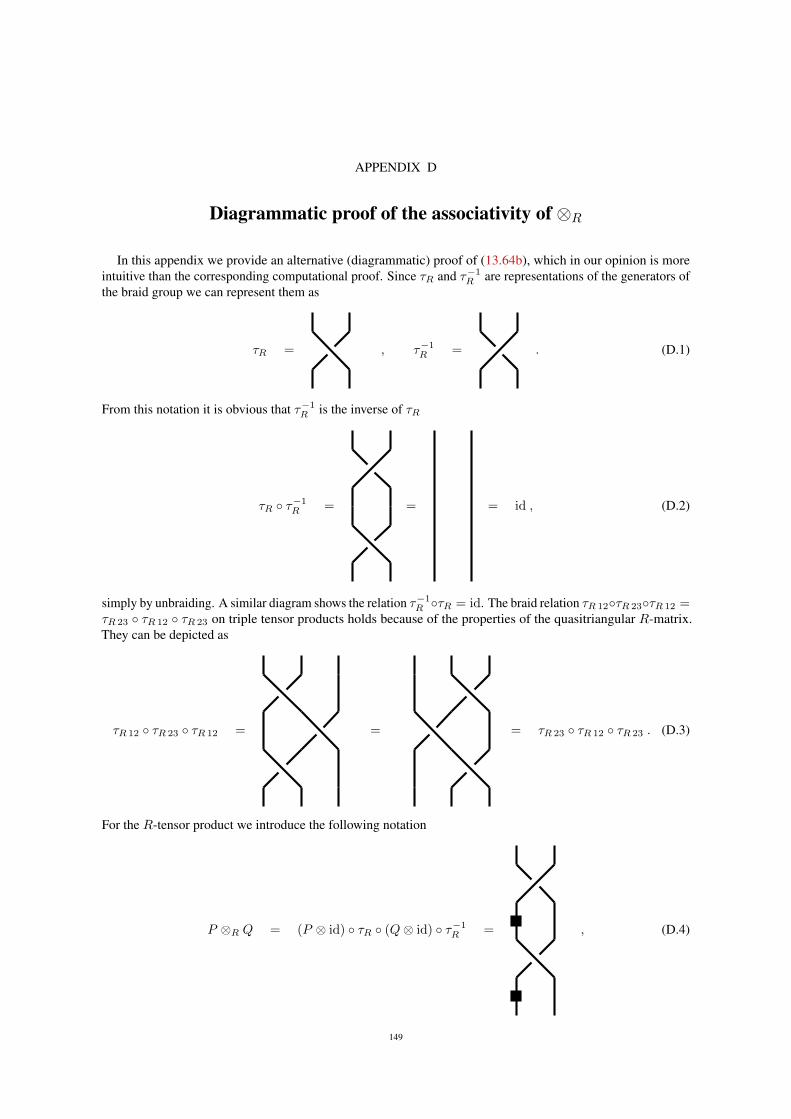
APPENDIX D

Diagrammatic proof of the associativity of ⊗R

In this appendix we provide an alternative (diagrammatic) proof of (13.64b), which in our opinion is moreintuitive than the corresponding computational proof. Since τR and τ−1

R are representations of the generators ofthe braid group we can represent them as

τR = , τ−1R = . (D.1)

From this notation it is obvious that τ−1R is the inverse of τR

τR τ−1R = = = id , (D.2)

simply by unbraiding. A similar diagram shows the relation τ−1R τR = id. The braid relation τR 12τR 23τR 12 =

τR 23 τR 12 τR 23 on triple tensor products holds because of the properties of the quasitriangular R-matrix.They can be depicted as

τR 12 τR 23 τR 12 = = = τR 23 τR 12 τR 23 . (D.3)

For the R-tensor product we introduce the following notation

P ⊗R Q = (P ⊗ id) τR (Q⊗ id) τ−1R = , (D.4)

149

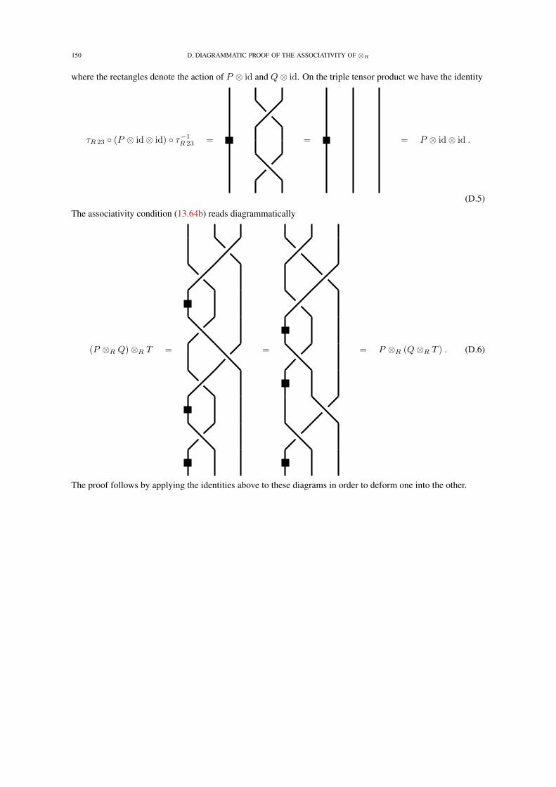
150 D. DIAGRAMMATIC PROOF OF THE ASSOCIATIVITY OF ⊗R

where the rectangles denote the action of P ⊗ id and Q⊗ id. On the triple tensor product we have the identity

τR 23 (P ⊗ id⊗ id) τ−1R 23 = = = P ⊗ id⊗ id .

(D.5)

The associativity condition (13.64b) reads diagrammatically

(P ⊗R Q)⊗R T = = = P ⊗R (Q⊗R T ) . (D.6)

The proof follows by applying the identities above to these diagrams in order to deform one into the other.

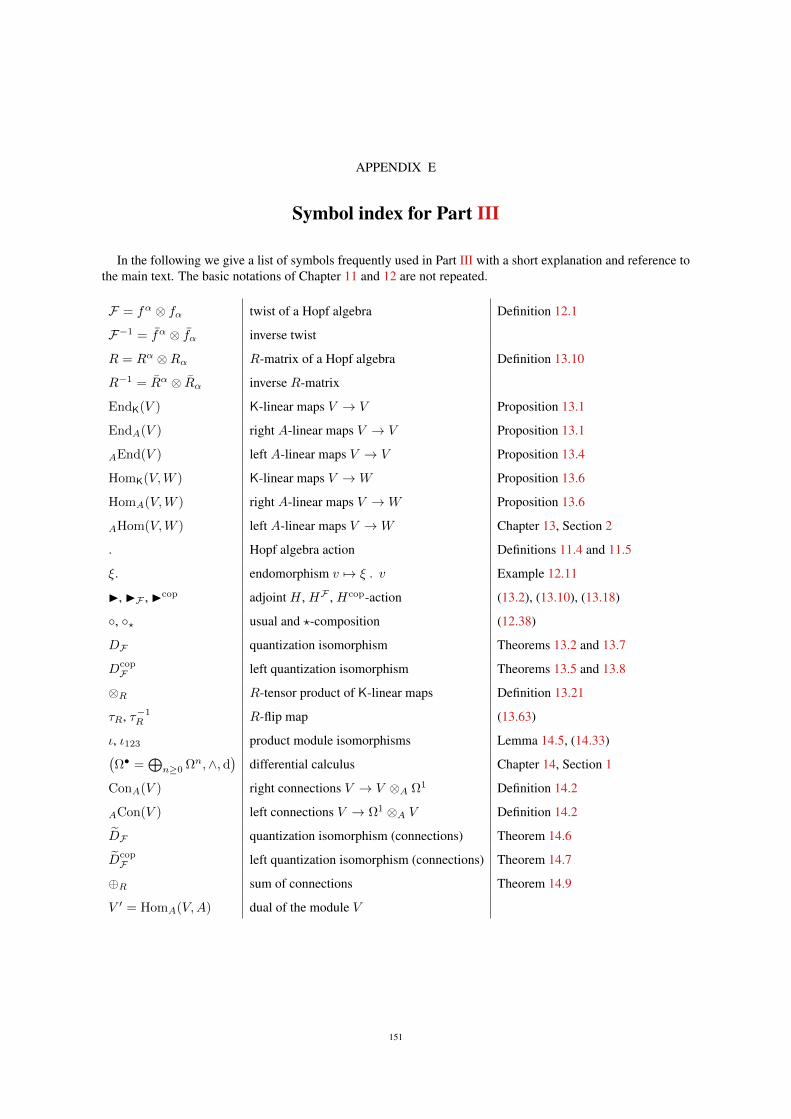
APPENDIX E

Symbol index for Part III

In the following we give a list of symbols frequently used in Part III with a short explanation and reference tothe main text. The basic notations of Chapter 11 and 12 are not repeated.

F = fα ⊗ fα twist of a Hopf algebra Definition 12.1

F−1 = fα ⊗ fα inverse twist

R = Rα ⊗Rα R-matrix of a Hopf algebra Definition 13.10

R−1 = Rα ⊗ Rα inverse R-matrix

EndK(V ) K-linear maps V → V Proposition 13.1

EndA(V ) right A-linear maps V → V Proposition 13.1

AEnd(V ) left A-linear maps V → V Proposition 13.4

HomK(V,W ) K-linear maps V →W Proposition 13.6

HomA(V,W ) right A-linear maps V →W Proposition 13.6

AHom(V,W ) left A-linear maps V →W Chapter 13, Section 2

. Hopf algebra action Definitions 11.4 and 11.5

ξ. endomorphism v 7→ ξ . v Example 12.11

I, IF , Icop adjoint H , HF , Hcop-action (13.2), (13.10), (13.18)

, ? usual and ?-composition (12.38)

DF quantization isomorphism Theorems 13.2 and 13.7

DcopF left quantization isomorphism Theorems 13.5 and 13.8

⊗R R-tensor product of K-linear maps Definition 13.21

τR, τ−1R R-flip map (13.63)

ι, ι123 product module isomorphisms Lemma 14.5, (14.33)(Ω• =

⊕n≥0 Ωn,∧,d

)differential calculus Chapter 14, Section 1

ConA(V ) right connections V → V ⊗A Ω1 Definition 14.2

ACon(V ) left connections V → Ω1 ⊗A V Definition 14.2

DF quantization isomorphism (connections) Theorem 14.6

DcopF left quantization isomorphism (connections) Theorem 14.7

⊕R sum of connections Theorem 14.9

V ′ = HomA(V,A) dual of the module V

151

Bibliography

[A+05] P. Aschieri et al., A gravity theory on noncommutative spaces, Class. Quant. Grav. 22, 3511–3532 (2005), [arXiv:hep-th/0504183].

[ABJ+08] E. Akofor, A. P. Balachandran, S. G. Jo, A. Joseph and B. A. Qureshi, Direction-Dependent CMB Power Spectrum andStatistical Anisotropy from Noncommutative Geometry, JHEP 05, 092 (2008), [arXiv:0710.5897].

[ABJ+09] E. Akofor, A. P. Balachandran, A. Joseph, L. Pekowsky and B. A. Qureshi, Constraints from CMB on Spacetime Noncom-mutativity and Causality Violation, Phys. Rev. D79, 063004 (2009), [arXiv:0806.2458].

[AC09a] P. Aschieri and L. Castellani, Noncommutative D=4 gravity coupled to fermions, JHEP 06, 086 (2009), [arXiv:0902.3817].[AC09b] P. Aschieri and L. Castellani, Noncommutative supergravity in D=3 and D=4, JHEP 06, 087 (2009), [arXiv:0902.3823].[AC10] P. Aschieri and L. Castellani, Noncommutative Gravity Solutions, J. Geom. Phys. 60, 375–393 (2010), [arXiv:0906.2774].[ADMW06] P. Aschieri, M. Dimitrijevic, F. Meyer and J. Wess, Noncommutative geometry and gravity, Class. Quant. Grav. 23,

1883–1912 (2006), [arXiv:hep-th/0510059].[AL98] J. Ambjorn and R. Loll, Non-perturbative Lorentzian quantum gravity, causality and topology change, Nucl. Phys. B536,

407–434 (1998), [arXiv:hep-th/9805108].[ALV08] P. Aschieri, F. Lizzi and P. Vitale, Twisting all the way: from Classical Mechanics to Quantum Fields, Phys. Rev. D77,

025037 (2008), [arXiv:0708.3002].[AOR06] A. Alboteanu, T. Ohl and R. Ruckl, Probing the noncommutative standard model at hadron colliders, Phys. Rev. D74,

096004 (2006), [arXiv:hep-ph/0608155].[AOR07] A. Alboteanu, T. Ohl and R. Ruckl, The Noncommutative Standard Model at O(θ2), Phys. Rev. D76, 105018 (2007),

[arXiv:0707.3595].[AS11] P. Aschieri and A. Schenkel, Twist deformations of module homomorphisms and connections, to appear (2011).[Asc09] P. Aschieri, Star Product Geometries, (2009), [arXiv:0903.2457].[Bah04] D. Bahns, Perturbative methods on the noncommutative Minkowski space, (2004), DESY-THESIS-2004-004.[Bah10] D. Bahns, The ultraviolet infrared mixing problem on the noncommutative Moyal space, (2010), [arXiv:1012.3707].[BDFP02] D. Bahns, S. Doplicher, K. Fredenhagen and G. Piacitelli, On the unitarity problem in space/time noncommutative theories,

Phys. Lett. B533, 178–181 (2002), [arXiv:hep-th/0201222].[BEE96] J. K. Beem, P. E. Ehrlich and K. L. Easley, Global Lorentzian geometry. 2nd ed., Pure and Applied Mathematics, Marcel

Dekker. 202. New York, NY: Marcel Dekker. xiv, 635 p. , 1996.[BF09] C. Bar, (ed. ) and K. Fredenhagen, (ed. ), Quantum field theory on curved spacetimes, Lect. Notes Phys. 786, 1–155 (2009).[BFF+78a] F. Bayen, M. Flato, C. Frønsdal, A. Lichnerowicz and D. Sternheimer, Deformation theory and quantization. I: Deformations

of symplectic structures., Ann. Phys. 111, 61–110 (1978).[BFF+78b] F. Bayen, M. Flato, C. Frønsdal, A. Lichnerowicz and D. Sternheimer, Deformation theory and quantization. II: Physical

applications., Ann. Phys. 111, 111–151 (1978).[BFK96] R. Brunetti, K. Fredenhagen and M. Kohler, The microlocal spectrum condition and Wick polynomials of free fields on

curved spacetimes, Commun. Math. Phys. 180, 633–652 (1996), [arXiv:gr-qc/9510056].[BGMTS04] A. P. Balachandran, T. R. Govindarajan, A. G. Martins and P. Teotonio-Sobrinho, Time-space noncommutativity: Quantised

evolutions, JHEP 11, 068 (2004), [arXiv:hep-th/0410067].[BGP07] C. Bar, N. Ginoux and F. Pfaffle, Wave equations on Lorenzian manifolds and quantization, (2007), Zuerich, Switzerland:

Eur. Math. Soc., 194 p.[BKSW10] D. N. Blaschke, E. Kronberger, R. I. P. Sedmik and M. Wohlgenannt, Gauge Theories on Deformed Spaces, SIGMA 6, 062

(2010), [arXiv:1004.2127].[BLS10] D. Buchholz, G. Lechner and S. J. Summers, Warped Convolutions, Rieffel Deformations and the Construction of Quantum

Field Theories, (2010), [arXiv:1005.2656].[BM10] E. Beggs and S. Majid, Nonassociative Riemannian geometry by twisting, Journal of Physics: Conference Series 254(1),

012002 (2010).[BM11] E. Beggs and S. Majid, *-compatible connections in noncommutative Riemannian geometry, Journal of Geometry and

Physics 61(1), 95 – 124 (2011).[BP68] H.-J. Borchers and K. Pohlmeyer, Eine scheinbare Abschwachung der Lokalitatsbedingung. II., Commun. Math. Phys. 8,

269–281 (1968).[BPQ08] A. P. Balachandran, A. Pinzul and B. A. Qureshi, Twisted Poincare Invariant Quantum Field Theories, Phys. Rev. D77,

025021 (2008), [arXiv:0708.1779].[BR87] O. Bratteli and D. W. Robinson, Operator algebras and quantum statistical mechanics. 1. C∗- and W ∗-algebras, symmetry

groups, decomposition of states. 2nd ed., Texts and Monographs in Physics. New York, NY: Springer. xiv, 505 p. , 1987.[BS05] A. N. Bernal and M. Sanchez, Smoothness of time functions and the metric splitting of globally hyperbolic spacetimes.,

Commun. Math. Phys. 257(1), 43–50 (2005).[BW98] M. Bordemann and S. Waldmann, Formal GNS construction and states in deformation quantization., Commun. Math. Phys.

195(3), 549–583 (1998).

153

154 BIBLIOGRAPHY

[CDPT01] M. Chaichian, A. Demichev, P. Presnajder and A. Tureanu, Space-time noncommutativity, discreteness of time and unitarity,Eur. Phys. J. C20, 767–772 (2001), [arXiv:hep-th/0007156].

[CFF93] A. H. Chamseddine, G. Felder and J. Frohlich, Gravity in noncommutative geometry, Commun. Math. Phys. 155, 205–218(1993), [arXiv:hep-th/9209044].

[CH99] C.-S. Chu and P.-M. Ho, Noncommutative open string and D-brane, Nucl. Phys. B550, 151–168 (1999), [arXiv:hep-th/9812219].

[Cha01] A. H. Chamseddine, Complexified gravity in noncommutative spaces, Commun. Math. Phys. 218, 283–292 (2001),[arXiv:hep-th/0005222].

[Cha04] A. H. Chamseddine, Sl(2,c) gravity with complex vierbein and its noncommutative extension, Phys. Rev. D69, 024015(2004), [arXiv:hep-th/0309166].

[CJS+02] X. Calmet, B. Jurco, P. Schupp, J. Wess and M. Wohlgenannt, The standard model on non-commutative space-time, Eur.Phys. J. C23, 363–376 (2002), [arXiv:hep-ph/0111115].

[CKNT04] M. Chaichian, P. P. Kulish, K. Nishijima and A. Tureanu, On a Lorentz-invariant interpretation of noncommutative space-timeand its implications on noncommutative QFT, Phys. Lett. B604, 98–102 (2004), [arXiv:hep-th/0408069].

[CL01] A. Connes and G. Landi, Noncommutative manifolds: The Instanton algebra and isospectral deformations, Com-mun.Math.Phys. 221, 141–159 (2001), [arXiv:math/0011194].

[Con94] A. Connes, Noncommutative geometry, (1994), Academic Press, San Diego, CA, 661 p.[CPT05] M. Chaichian, P. Presnajder and A. Tureanu, New concept of relativistic invariance in NC space-time: Twisted Poincare

symmetry and its implications, Phys. Rev. Lett. 94, 151602 (2005), [arXiv:hep-th/0409096].[DF99] M. Duetsch and K. Fredenhagen, A local (perturbative) construction of observables in gauge theories: The example of QED,

Commun. Math. Phys. 203, 71–105 (1999), [arXiv:hep-th/9807078].[DFR94] S. Doplicher, K. Fredenhagen and J. E. Roberts, Spacetime quantization induced by classical gravity, Physics Letters B

331(1-2), 39 – 44 (1994).[DFR95] S. Doplicher, K. Fredenhagen and J. E. Roberts, The Quantum structure of space-time at the Planck scale and quantum fields,

Commun. Math. Phys. 172, 187–220 (1995), [arXiv:hep-th/0303037].[DGMR07] M. Disertori, R. Gurau, J. Magnen and V. Rivasseau, Vanishing of beta function of non commutative phi(4)**4 theory to all

orders, Phys. Lett. B649, 95–102 (2007), [arXiv:hep-th/0612251].[DGS07] B. P. Dolan, K. S. Gupta and A. Stern, Noncommutative BTZ black hole and discrete time, Class. Quant. Grav. 24,

1647–1656 (2007), [arXiv:hep-th/0611233].[DHP09] C. Dappiaggi, T.-P. Hack and N. Pinamonti, The extended algebra of observables for Dirac fields and the trace anomaly of

their stress-energy tensor, Rev. Math. Phys. 21, 1241–1312 (2009), [arXiv:0904.0612].[DLMM11] C. Dappiaggi, G. Lechner and E. Morfa-Morales, Deformations of quantum field theories on spacetimes with Killing vector

fields, Commun. Math. Phys. 305, 99–130 (2011), [arXiv:1006.3548].[DP10] L. Dabrowski and G. Piacitelli, Canonical k-Minkowski Spacetime, (2010), [arXiv:1004.5091].[DV01] M. Dubois-Violette, Lectures on graded differential algebras and noncommutative geometry., Maeda, Yoshiaki (ed.) et al.,

Noncommutative differential geometry and its applications to physics. Proceedings of the workshop, Shonan, Japan, May31–June 4, 1999. Dordrecht: Kluwer Academic Publishers. Math. Phys. Stud. 23, 245-306 (2001)., 2001.

[Ear74] D. M. Eardley, Self-similar spacetimes: geometry and dynamics, Commun. Math. Phys. 37, 287–309 (1974).[FS09] A. Fischer and R. J. Szabo, Duality covariant quantum field theory on noncommutative Minkowski space, JHEP 02, 031

(2009), [arXiv:0810.1195].[FS10] A. Fischer and R. J. Szabo, UV/IR duality in noncommutative quantum field theory, (2010), [arXiv:1001.3776].[GL07] H. Grosse and G. Lechner, Wedge-Local Quantum Fields and Noncommutative Minkowski Space, JHEP 11, 012 (2007),

[arXiv:0706.3992].[GL08] H. Grosse and G. Lechner, Noncommutative Deformations of Wightman Quantum Field Theories, JHEP 09, 131 (2008),

[arXiv:0808.3459].[GM94] D. Gurevich and S. Majid, Braided groups of Hopf algebras obtained by twisting., Pac. J. Math. 162(1), 27–44 (1994).[GMRVT06] R. Gurau, J. Magnen, V. Rivasseau and F. Vignes-Tourneret, Renormalization of non-commutative phi**4(4) field theory in

x space, Commun. Math. Phys. 267, 515–542 (2006), [arXiv:hep-th/0512271].[GN94] I. Gelfand and M. Neumark, On the imbedding of normed rings into the ring of operators in Hilbert space., Doran, Robert

S. (ed.), C∗-Algebras: 1943-1993. A fifty year celebration. AMS special session commemorating the first fifty years ofC∗-algebra theory, January 13-14, 1993, San Antonio, TX, USA. Providence, RI: American Mathematical Society. Contemp.Math. 167, 3-20 (1994)., 1994.

[GR09] R. Gurau and O. J. Rosten, Wilsonian Renormalization of Noncommutative Scalar Field Theory, JHEP 07, 064 (2009),[arXiv:0902.4888].

[GW04] H. Grosse and R. Wulkenhaar, The beta-function in duality-covariant noncommutative phi**4 theory, Eur. Phys. J. C35,277–282 (2004), [arXiv:hep-th/0402093].

[GW05a] H. Grosse and R. Wulkenhaar, Power-counting theorem for non-local matrix models and renormalisation, Commun. Math.Phys. 254, 91–127 (2005), [arXiv:hep-th/0305066].

[GW05b] H. Grosse and R. Wulkenhaar, Renormalisation of phi**4 theory on noncommutative R**4 in the matrix base, Commun.Math. Phys. 256, 305–374 (2005), [arXiv:hep-th/0401128].

[GW09] H. Grosse and R. Wulkenhaar, Progress in solving a noncommutative quantum field theory in four dimensions, (2009),[arXiv:0909.1389].

[HKM04] I. Hinchliffe, N. Kersting and Y. L. Ma, Review of the phenomenology of noncommutative geometry, Int. J. Mod. Phys.A19, 179–204 (2004), [arXiv:hep-ph/0205040].

[Hor90] L. Hormander, The analysis of linear partial differential operators. I. Distribution theory and Fourier analysis. 2nd ed.,Grundlehren der Mathematischen Wissenschaften, 256. Berlin etc.: Springer-Verlag. xi, 440 p. , 1990.

[Hor09] P. Horava, Quantum Gravity at a Lifshitz Point, Phys. Rev. D79, 084008 (2009), [arXiv:0901.3775].[HPR01] J. L. Hewett, F. J. Petriello and T. G. Rizzo, Signals for non-commutative interactions at linear colliders, Phys. Rev. D64,

075012 (2001), [arXiv:hep-ph/0010354].

BIBLIOGRAPHY 155

[JMS+01] B. Jurco, L. Moller, S. Schraml, P. Schupp and J. Wess, Construction of non-Abelian gauge theories on noncommutativespaces, Eur. Phys. J. C21, 383–388 (2001), [arXiv:hep-th/0104153].

[JS04] C. Jambor and A. Sykora, Realization of algebras with the help of *-products, (2004), [arXiv:hep-th/0405268].[Kas95] C. Kassel, Quantum groups, (1995), New York, USA: Springer (1995) 531 p. (Graduate text in mathematics, 155).[KM11] T. S. Koivisto and D. F. Mota, CMB statistics in noncommutative inflation, JHEP 02, 061 (2011), [arXiv:1011.2126].[KS07] S. Kurkcuoglu and C. Saemann, Drinfeld twist and general relativity with fuzzy spaces, Class. Quant. Grav. 24, 291–312

(2007), [arXiv:hep-th/0606197].[KYR05] H.-C. Kim, J. H. Yee and C. Rim, Density fluctuations in kappa-deformed inflationary universe, Phys. Rev. D72, 103523

(2005), [arXiv:gr-qc/0506122].[Lam99] T. Lam, Lectures on modules and rings., Graduate Texts in Mathematics. 189. New York, NY: Springer. xxiii, 557 p. , 1999.[LMMP02] F. Lizzi, G. Mangano, G. Miele and M. Peloso, Cosmological perturbations and short distance physics from noncommutative

geometry, JHEP 06, 049 (2002), [arXiv:hep-th/0203099].[LvS06] G. Landi and W. van Suijlekom, Noncommutative bundles and instantons in tehran, pages 275–353 (2006), [arXiv:hep-

th/0603053].[Mad00] J. Madore, An introduction to noncommutative differential geometry and itsphysical applications, Lond.Math.Soc.Lect.Note

Ser. 257, 1–371 (2000).[Maj95] S. Majid, Foundations of quantum group theory, (1995), Cambridge, UK: Univ. Pr., 607 p.[MH08] F. Muller-Hoissen, Noncommutative Geometries and Gravity, AIP Conf. Proc. 977, 12–29 (2008), [arXiv:0710.4418].[MPKT+05a] B. Melic, K. Passek-Kumericki, J. Trampetic, P. Schupp and M. Wohlgenannt, The standard model on non-commutative

space-time: Electroweak currents and Higgs sector, Eur. Phys. J. C42, 483–497 (2005), [arXiv:hep-ph/0502249].[MPKT+05b] B. Melic, K. Passek-Kumericki, J. Trampetic, P. Schupp and M. Wohlgenannt, The standard model on non-commutative

space-time: Strong interactions included, Eur. Phys. J. C42, 499–504 (2005), [arXiv:hep-ph/0503064].[O’N83] B. O’Neill, Semi-Riemannian geometry. With applications to relativity., Pure and Applied Mathematics, 103. New York-

London etc.: Academic Press. XIII, 468 p. , 1983.[OR04] T. Ohl and J. Reuter, Testing the noncommutative standard model at a future photon collider, Phys. Rev. D70, 076007

(2004), [arXiv:hep-ph/0406098].[OS09a] T. Ohl and A. Schenkel, Cosmological and Black Hole Spacetimes in Twisted Noncommutative Gravity, JHEP 10, 052

(2009), [arXiv:0906.2730].[OS09b] T. Ohl and A. Schenkel, Symmetry Reduction in Twisted Noncommutative Gravity with Applications to Cosmology and

Black Holes, JHEP 01, 084 (2009), [arXiv:0810.4885].[OS10] T. Ohl and A. Schenkel, Algebraic approach to quantum field theory on a class of noncommutative curved spacetimes, Gen.

Rel. Grav. 42, 2785–2798 (2010), [arXiv:0912.2252].[OSU10] T. Ohl, A. Schenkel and C. F. Uhlemann, Spacetime Noncommutativity in Models with Warped Extradimensions, JHEP 07,

029 (2010), [arXiv:1002.2884].[Poh68] K. Pohlmeyer, Eine scheinbare Abschwachung der Lokalitatsbedingung., Commun. Math. Phys. 7, 80–92 (1968).[Pol05a] J. Polchinski, String theory. Vol I: An introduction to the bosonic string. 1st paperback edition., Cambridge: Cambridge

University Press; Washington, DC: The Mathematical Association of America (MAA). xix, 402 p. , 2005.[Pol05b] J. Polchinski, String theory. Vol II: superstring theory and beyond. 1st paperback edition., Cambridge: Cambridge University

Press; Washington, DC: The Mathematical Association of America (MAA). xix, 531 p. , 2005.[PV04] M. Paschke and R. Verch, Local covariant quantum field theory over spectral geometries, Class. Quant. Grav. 21, 5299–5316

(2004), [arXiv:gr-qc/0405057].[Rad96] M. J. Radzikowski, Micro-local approach to the Hadamard condition in quantum field theory on curved space-time, Commun.

Math. Phys. 179, 529–553 (1996).[Res90] N. Reshetikhin, Multiparameter quantum groups and twisted quasitriangular Hopf algebras, Lett. Math. Phys. 20, 331–335

(1990).[Reu98] M. Reuter, Nonperturbative Evolution Equation for Quantum Gravity, Phys. Rev. D57, 971–985 (1998), [arXiv:hep-

th/9605030].[Rie93] M. A. Rieffel, Deformation quantization for actions of Rd., Mem. Am. Math. Soc. 506, 93 p. (1993).[Riv03] V. O. Rivelles, Noncommutative field theories and gravity, Phys. Lett. B558, 191–196 (2003), [arXiv:hep-th/0212262].[Rov07] C. Rovelli, Quantum gravity. 1st paperback ed., Cambridge Monographs on Mathematical Physics. Cambridge: Cambridge

University Press. xxiii, 455 p. , 2007.[RS99] L. Randall and R. Sundrum, A large mass hierarchy from a small extra dimension, Phys. Rev. Lett. 83, 3370–3373 (1999),

[arXiv:hep-ph/9905221].[RVTW06] V. Rivasseau, F. Vignes-Tourneret and R. Wulkenhaar, Renormalization of noncommutative phi**4-theory by multi- scale

analysis, Commun. Math. Phys. 262, 565–594 (2006), [arXiv:hep-th/0501036].[Sch99] V. Schomerus, D-branes and deformation quantization, JHEP 06, 030 (1999), [arXiv:hep-th/9903205].[Sch09] A. Schenkel, Symmetry Reduction and Exact Solutions in Twisted Noncommutative Gravity, Acta Phys. Polon. B Proc. Suppl.

2, 657 (2009), [arXiv:0908.0434].[Sch10] A. Schenkel, Quantum Field Theory on Curved Noncommutative Spacetimes, PoS CNCFG2010, 029 (2010),

[arXiv:1101.3492].[Sch11] A. Schenkel, QFT on homothetic Killing twist deformed curved spacetimes, accepted by General Relativity and Gravitation

(2011), [arXiv:1009.1090].[Ser55] J.-P. Serre, Faisceaux algebriques coherents., (1955).[SK10] A. Sfondrini and T. A. Koslowski, Functional Renormalization of Noncommutative Scalar Field Theory, (2010),

[arXiv:1006.5145].[SS07] P. Schupp and S. Solodukhin, Exact Black Hole Solutions in Noncommutative Gravity, (2007), talk at:

International Conference Noncommutative Geometry & Physics NPT Orsay, April 23-27, 2007http://www.th.u-psud.fr/page_perso/Rivasseau/NONCOM07/;Bayrischzell workshop on non-commutativity and physics, May 11-14, 2007

156 BIBLIOGRAPHY

http://homepage.univie.ac.at/michael.wohlgenannt/bzell/Bayrischzell_Workshop_2007.html;4th Vienna Central European Seminar on Particle Physics and Quantum Field Theory, November 30 - December 02, 2007http://www.univie.ac.at/vienna.seminar/2007/abstracts/abstr_Schupp.html.

[SS09] P. Schupp and S. Solodukhin, Exact Black Hole Solutions in Noncommutative Gravity, (2009), [arXiv:0906.2724].[Ste07] H. Steinacker, Emergent Gravity from Noncommutative Gauge Theory, JHEP 12, 049 (2007), [arXiv:0708.2426].[Ste09] H. Steinacker, Emergent Gravity and Noncommutative Branes from Yang-Mills Matrix Models, Nucl. Phys. B810, 1–39

(2009), [arXiv:0806.2032].[Ste10] H. Steinacker, Emergent Geometry and Gravity from Matrix Models: an Introduction, Class. Quant. Grav. 27, 133001

(2010), [arXiv:1003.4134].[SU10a] A. Schenkel and C. F. Uhlemann, Field Theory on Curved Noncommutative Spacetimes, SIGMA 6, 061 (2010),

[arXiv:1003.3190].[SU10b] A. Schenkel and C. F. Uhlemann, High energy improved scalar quantum field theory from noncommutative geometry without

UV/IR-mixing, Phys. Lett. B694, 258–260 (2010), [arXiv:1002.4191].[SW99] N. Seiberg and E. Witten, String theory and noncommutative geometry, JHEP 09, 032 (1999), [arXiv:hep-th/9908142].[Swa62] R. Swan, Vector bundles and projective modules., Trans. Am. Math. Soc. 105, 264–277 (1962).[Sza06] R. J. Szabo, Symmetry, gravity and noncommutativity, Class. Quant. Grav. 23, R199–R242 (2006), [arXiv:hep-th/0606233].[Thi07] T. Thiemann, Modern canonical quantum general relativity., Cambridge Monographs on Mathematical Physics. Cambridge:

Cambridge University Press. xxvi, 819 p. , 2007.[Wal94] R. M. Wald, Quantum field theory in curved space-time and black hole thermodynamics, (1994), Chicago, USA: Univ. Pr.,

205 p.[Wal05] S. Waldmann, States and representations in deformation quantization., Rev. Math. Phys. 17(1), 15–75 (2005).[Wal07] S. Waldmann, Poisson geometry and deformation quantisation. An introduction. (Poisson-Geometrie und Deformations-

quantisierung. Eine Einfuhrung.), Berlin: Springer. xii, 612 p. EUR 39.95; SFR 65.50 , 2007.[Wor89] S. L. Woronowicz, Differential calculus on compact matrix pseudogroups (quantum groups), Commun. Math. Phys. 122,

125–170 (1989).[Yan07] H. S. Yang, On The Correspondence Between Noncommuative Field Theory And Gravity, Mod. Phys. Lett. A22, 1119–1132

(2007), [arXiv:hep-th/0612231].[Yan09] H. S. Yang, Emergent gravity from noncommutative spacetime, Int. J. Mod. Phys. A24, 4473–4517 (2009), [arXiv:hep-

th/0611174].[YF50] C.-N. Yang and D. Feldman, The S matrix in the Heisenberg representation, Phys. Rev. 79, 972–978 (1950).[Zah06a] J. Zahn, Remarks on twisted noncommutative quantum field theory, Phys. Rev. D73, 105005 (2006), [arXiv:hep-th/0603231].[Zah06b] J. W. Zahn, Dispersion relations in quantum electrodynamics on the noncommutative Minkowski space, (2006),

[arXiv:0707.2149].[Zah10] J. Zahn, Noncommutative (supersymmetric) electrodynamics in the Yang-Feldman formalism, Phys. Rev. D82, 105033

(2010), [arXiv:1008.2309].[Zah11a] J. Zahn, Divergences in quantum field theory on the noncommutative two-dimensional Minkowski space with Grosse-

Wulkenhaar potential, Annales Henri Poincare 12, 777–804 (2011), [arXiv:1005.0541].[Zah11b] J. Zahn, Ultraviolet-infrared mixing on the noncommutative Minkowski space in the Yang-Feldman formalism, (2011),

[arXiv:1105.6240].

Acknowledgements

I would like to thank my friends, colleagues and collaborators for their support during my PhD thesis. A particularthanks goes to:

• Prof. Dr. Thorsten Ohl for the opportunity to write my thesis in his group, the many discussions andthe fruitful collaborations.

• Dr. Paolo Aschieri, Dr. Tim Koslowski and Christoph Uhlemann for many discussions and fruitfulcollaborations.

• Prof. Dr. Christian Klingenberg and Prof. Dr. Werner Porod for joining my “Betreuungskommission”.

• Prof. Dr. Haye Hinrichsen and Prof. Dr. Peter Schupp for agreeing to be a referee for my thesis.

• All members of Theoretical Physics II and the Research Training Group GRK 1147 for the interestingand nice time. In particular Julian Adamek for keeping alive my interest in cosmology.

• Dr. Paolo Aschieri, Prof. Dr. Dorothea Bahns, Dr. Daniel Blaschke, Prof. Dr. Leonardo Castellani,Dr. Claudio Dappiaggi, Dr. Marija Dimitrijevic, Prof. Dr. Klaus Fredenhagen, Prof. Dr. Harald Grosse,Dr. Gandalf Lechner, Prof. Dr. John Madore, Eric Morfa-Morales, Prof. Dr. Denjoe O’Connor, Prof. Dr.Jeong-Hyuck Park, Dr. Christian Samann, Prof. Dr. Martin Schlichenmaier, Paul Schreivogl, Prof. Dr.Peter Schupp, PD Dr. Harold Steinacker, Dr. Christoph Stephan, Prof. Dr. Richard Szabo, Prof. Dr.Dmitri Vassilevich, Prof. Dr. Rainer Verch, Prof. Dr. Stefan Waldmann, Dr. Michael Wohlgenannt,Dr. Hyun Seok Yang and Dr. Jochen Zahn, not only for many discussions and helpful comments, butalso for the enjoyable “social events” during conferences.

• Quantum Geometry and Quantum Gravity Network of the European Science Foundation (ESF) for thefinancial support.

• Perimeter Institute for Theoretical Physics for the invitation and the financial support.

• Research Training Group 1147 Theoretical Astrophysics and Particle Physics of the DFG for thefinancial support.

• Brigitte Wehner for helping me with all sorts of bureaucracy.

• My parents, family and “non-physics friends” for the support and enjoyable free time.

• And last but not least Asma Cheriguene for giving me her love, support and the valuable time together.

Thanks!

157

List of publications

Articles in peer reviewed journals:

[1] A. Schenkel,“QFT on homothetic Killing twist deformed curved spacetimes”,Gen. Rel. Grav. 43, 2605 (2011) [arXiv:1009.1090 [math-ph]].

[2] A. Schenkel and C. F. Uhlemann,“High energy improved scalar quantum field theory from noncommutative geometrywithout UV/IR-mixing”,Phys. Lett. B 694, 258 (2010) [arXiv:1002.4191 [hep-th]].

[3] T. Ohl, A. Schenkel and C. F. Uhlemann,“Spacetime Noncommutativity in Models with Warped Extradimensions”,JHEP 1007, 029 (2010) [arXiv:1002.2884 [hep-th]].

[4] T. Ohl and A. Schenkel,“Algebraic approach to quantum field theory on a class of noncommutative curved spacetimes”,Gen. Rel. Grav. 42, 2785 (2010) [arXiv:0912.2252 [hep-th]].

[5] T. Koslowski and A. Schenkel,“Preferred foliation effects in Quantum General Relativity”,Class. Quant. Grav. 27, 135014 (2010) [arXiv:0910.0623 [gr-qc]].

[6] T. Ohl and A. Schenkel,“Cosmological and Black Hole Spacetimes in Twisted Noncommutative Gravity”,JHEP 0910, 052 (2009) [arXiv:0906.2730 [hep-th]].

[7] T. Ohl and A. Schenkel,“Symmetry Reduction in Twisted Noncommutative Gravity with Applications to Cosmologyand Black Holes”,JHEP 0901, 084 (2009) [arXiv:0810.4885 [hep-th]].

Invited review articles:

[8] A. Schenkel and C. F. Uhlemann,“Field Theory on Curved Noncommutative Spacetimes”,SIGMA 6, 061 (2010) [arXiv:1003.3190 [hep-th]].

Conference and workshop proceedings:

[9] A. Schenkel,“Quantum Field Theory on Curved Noncommutative Spacetimes”,PoS(CNCFG2010)029 [arXiv:1101.3492 [hep-th]],“Noncommutative Field Theory and Gravity”, September 2010, Corfu.

[10] A. Schenkel,“Quantum Field Theory on Noncommutative Curved Spacetimes”,in Oberwolfach Reports No. 43/2010,“Deformation Methods in Mathematics and Physics”, September 2010, MFO Oberwolfach.

[11] A. Schenkel,“Symmetry Reduction and Exact Solutions in Twisted Noncommutative Gravity”,Acta Phys. Polon. B Proc. Suppl. 2: 657 (2009) [arXiv:0908.0434 [hep-th]],“Non-perturbative Gravity and Quantum Chromodynamics”, June 2009, Zakopane.

159

Lebenslauf

Personliche Details:

Name: Alexander Schenkel

Geburtstag: 21. August 1983

Geburtsort: Hardheim, Deutschland

Familienstand: Ledig, keine Kinder

Staatsangehorigkeit: Deutsch

Schulbildung:

09/1994-06/2003 Deutschhaus Gymnasium, Wurzburg

Qualifikation: Abitur

09/1990-07/1994 Grundschule, Helmstadt

Universitatsbildung:

seit 06/2008 Doktorand, Universitat Wurzburg

Betreuer: Prof. Dr. Thorsten Ohl

Mitglied des Graduiertenkollegs GRK1147“Theoretical Astrophysics and Particle Physics”

08/2005-06/2008 Hauptstudium Physik, Universitat Wurzburg

Diplomarbeit: (Betreuer: Prof. Dr. Thorsten Ohl)“Pseudo-local Dirac observables in effective theories of quantum gravity”

Qualifikation: Diplom (mit Auszeichnung)

10/2003-08/2005 Grundstudium Physik, Universitat Wurzburg

Qualifikation: Vordiplom (mit Auszeichnung)

Wurzburg, den 14. Juni 2011

161

Erklarung

Diese Doktorarbeit wurde am Lehrstuhl fur Theoretische Physik II, Theoretische Elementarteilchenphysik,der Julius-Maximilians-Universitat Wurzburg angefertigt.Ich erklare hiermit, dass ich diese Dissertation selbstandig verfasst und keine anderen als die angegebenenQuellen und Hilfsmittel benutzt habe.Ich erklare außerdem, dass diese Dissertation weder in gleicher noch in anderer Form bereits in einem anderenPrufungsverfahren vorgelegen hat.Ich habe fruher außer den mit dem Zulassungsgesuch urkundlich vorgelegten Graden keine weiteren akademis-chen Grade erworben oder zu erwerben versucht.

Alexander SchenkelWurzburg, den 14. Juni 2011

163