Embed Size (px)
Citation preview

The noncommutative geometry of the quantum Hall effect J. Bellissard;a) A. van Elst,b) and H. Schulz- Baldest) Universid Paul Sabatiel; Toulouse, Framed)
(Received 1 May 1994; accepted for publication 17 May 1994)
An overview of the integer quantum Hall effect is given. A mathematical frame- work using nonommutative geometry as defined by Connes is prepared. Within this framework, it is proved that the Hall conductivity is quantized and that plateaux occur when the Fermi energy varies in a region of localized states.
TABLE OF CONTENTS
I. INTRODUCTION .......................................................... 5374 II. IQHE: EXPERIMENTS AND THEORIES. .................................... 5375
A. The classical Hall effect. ................................................. 5375 B. The quantum Hall effect. ................................................ 5377 C. The Hall effect for the free Fermi gas. ..................................... 5379 D. The role of localization. ................................................. 5380 E. The Laughlin argument. ................................................. 5382 F. The Chern-Kubo relationship. ............................................ 5384
III. THE NONCOMMUTATIVE GEOMETRY OF THE IQHE. ..................... 5387 A. The noncommutative Brillouin zone. ....................................... 5387 B. Hall conductance and noncommutative Chem character. ....................... 5389 C. Localization and plateaux of the Hall conductance. ........................... 5390 D. Summary of the main results. ............................................. 5392 E. Homogeneous Schrodinger’s operators. ..................................... 5393 F. Observables and calculus. ................................................ 5395
IV. THE KUBO-CHERN FORMULA. .......................................... 5399 A. The relaxation time approximation. ........................................ 5399 B. Kubo’s formula ......................................................... 5403 C. Estimating the deviations from the IQHE limit. .............................. 5405 D. Dixmier trace and Sobolev space. .......................................... 5408 E. Noncommutative Chem character. ......................................... 5412 E Connes formulas ........................................................ 5414 G. Chem character and Fredholm index. ...................................... 5417 H. Quantization, Fredholm and relative index. .................................. 5419
V. LOCALIZATION AND NONCOMMUTATIVE SOBOLEV SPACE. ............... 5420 A. The Anderson-Pastur localization criterion. ................................. 5420 B. Noncommutative localization criterion and localization length. .................. 5423 C. Localization in physical models. .......................................... 5429
VI. APPLICATIONS AND COMPLEMENTS. ................................... 5431 A. Low-lying states do not contribute to the IQHE. ............................. 5431 B. Where and how does the localization length diverge?. ......................... 5432 C. Chem numbers and localization in Harper’s equation. ......................... 5433
VII. INTRODUCTION TO THE FQHE ......................................... 5436 A. Ove~iew .............................................................. 5436 B. Laughlin’s ansatz for the v= l/m ground state. ............................... 5437 C. The elementary theory of the v=l/m-FQHE. ................................ 5442 D. The role of gauge invariance and incompressibility. ........................... 5443
0022-2466/94/35(10)/5373/79/$6.00 J. Math. Phys. 35 (lo), October 1994 8 1994 American Institute of Physics 5373
Downloaded 09 May 2005 to 128.32.113.135. Redistribution subject to AIP license or copyright, see http://jmp.aip.org/jmp/copyright.jsp
5374 Bellissard, van Elst, and Schulz-Baldes: Noncommutative geometry of quantum Hall effect
I. INTRODUCTION
In 1880, Hall’ undertook the classical experiment which led to the so-called Hall effect. A century later, von Klitzing and his co-workers* showed that the Hall conductivity was quantized at very low temperatures as an integer multiple of the universal constant e*/h. Here e is the electron charge whereas h is Planck’s constant. This is the integer quantum Hall effect (IQHE). For this discovery, which led to a new accurate measurement of the fine structure constant and a new definition of the standard of resistance,3 von Klitzing was awarded the Nobel price in 1985.
On the other hand, during the seventies, Connes4V5 extended most of the tools of differential geometry to noncommutative C*-algebras, thus creating a new branch of mathematics called Noncommutative Geometry. The main new result obtained in this field was the definition of cyclic cohomology and the proof of an index theorem for elliptic operators on a foliated manifold. For this work and also his contribution to the study of von Neumann algebras, Connes was awarded the Fields Medal in 1982. He recently extended this theory to what is now called Quantum Calculus.6
After the works by Laughlin7 and especially by Kohmoto, den Nijs, Nightingale, and Thouless’ (called TKN, below), it became clear that the quantization of the Hall conductance at low temperature had a geometric origin. The universality of this effect had then an explanation. Moreover, as proposed by Prange,“” Thouless,” and Halperin,51 the plateaux of the Hall conduc- tance which appear while changing the magnetic field or the charge-carrier density, are due to localization. Neither the original Laughlin paper nor the TKN2 one however could give a descrip- tion of both properties in the same model. Developing a mathematical framework able to reconcile topological and localization properties at once was a challenging problem. Attempts were made by Avron et al.‘* who exhibited quantization but were not able to prove that these quantum numbers were insensitive to disorder. In 1986, Kunz13 went further on and managed to prove this for disorder small enough to avoid filling the gaps between Landau levels.
But in Refs. 14-16 one of us proposed to use noncommutative geometry to extend the TKN, argument to the case of arbitrary magnetic field and disordered crystal. It turned out that the condition under which plateaux occur was precisely the finiteness of the localization length near the Fermi level. This work was rephrased later on by Avron et aLI7 in terms of charge transport and relative index, filling the remaining gap between experimental observations, theoretical intu- ition and mathematical frame.
Our aim in this work is to review these various contributions in a synthetic and detailed way. We will use this opportunity to give proofs that are missing or scattered in the literature. In addition, we will discuss the effect of disorder from two complementary aspects.
On the one hand, we will develop our point of view on localization produced by quenched disorder. This is crucial for understanding the IQHE. We review various localization criteria and formulate them in terms of noncommutative geometry. With the Dixmier trace, Connes introduced a remarkable technique into quantum calculus. In our context, it allows us to give the precise condition under which the Hall conductance is quantized; this condition is shown to be a local- ization condition.
On the other hand, we also propose a model for electronic transport giving rise to the so-called “relaxation time approximation” and allowing to derive a Kubo formula for the conductivity. This approach allows us to describe the effect of time-dependent disorder in a phenomenological way. This latter has quite different consequences from those of the quenched disorder such as a nonzero finite direct conductivity. Even though this approach is not original in its principle, the noncom- mutative framework allows us to treat the case of aperiodic crystals and magnetic fields when Bloch theory fails. Therefore, strictly speaking, our Kubo formula is new. We also show, without proofs, how to justify the linear response theory within this framework, leaving the formal proofs for a future work. The advantage of this approach is to give control of the various approximations that have to be made to fit the ideal result with experiments. For this reason, we discuss the effects of temperature, of nonlinear terms in the electric field, of the finite size of samples and finally
J. Math. Phys., Vol. 35, No. 10, October 1994
Downloaded 09 May 2005 to 128.32.113.135. Redistribution subject to AIP license or copyright, see http://jmp.aip.org/jmp/copyright.jsp
Bellissard, van Elst, and Schulz-Baldes: Noncommutative geometry of quantum Hall effect 5375
those of collisions and disorder. In particular, we argue that the discrepancy 6~~ between the measured Hall conductivity and the ideal one, given by a Chem number, is dominated by the collision terms. In the center of a plateau, we get the rough estimate
SCH e X2 - Gconst v- - ,
UH h I-Q (1)
where v is the filling factor, X is the localization length, and ,u~ is the charge-carrier mobility. e/h is a universal constant, v about unity and the localization length typically of the order of the magnetic length. Inserting measured values for the mobility, one obtains 10e4 for the right-hand side expression. This estimate does not take into account the Mott conductivity. However, it shows why both a large quenched disorder (in order to have small localization lengths) and a large mobility (namely, a low collision rate) are necessary in order to get accurate measurements. Such a compromise is realized in heterojunctions and to less extent in MOSEETs. The estimate (1) also permits us to understand intuitively why the plateaux in the fractional quantum Hall effect (FQHE) are less precise, since the localization length of Laughlin quasiparticles is probably larger than that of electrons at integer plateaux, and their mobility probably lower.
No attempt will be made however to extend our noncommutative approach to the FQHE. We will only give some insight and a short review of works that we feel relevant in view of a mathematically complete description of the FQHE.
This rest of the article is organized as follows. In Sec. II we give the conventional explana- tions of the IQHE. In particular, we discuss the Laughlin argument, the topological aspect intro- duced by TKN2 and the effects of localization in a qualitative way. Section III is devoted to the mathematical framework needed for noncommutative geometry. In particular we describe how to overcome the difficulty of not having Bloch’s theorem for aperiodic media. We then show that the Brillouin zone still exists as a noncommutative manifold. We also give the main steps of our strategy leading to a complete mathematical description of the IQHE. In Sec. IV we discuss transport theory leading to Kubo’s formula. We show that in the IQHE idealization, the Hall conductance is a noncommutative Chem number. We also relate this Chern number to a Fredholm index which leads to the quantization of the Hall conductance. Through the notion of relative index we show in which sense this approach is a rigorous version of the Laughlin argument. Section V is devoted to localization theory. We give various criteria and define various localization lengths which are commonly used in the literature. We also show how to express these notions in the n&commutative language. This part allows us to explain on a rigorous basis the occurrence of plateaux of the Hall conductance. Finally, we show that such criteria are in fact satisfied in models such as the Anderson model. In Sec. VI we give some consequences of this theory for practical models. In particular we show that low-lying states do not contribute to the IQHE. We also discuss the open question where the jumps of the Hall conductance occur. Section VII is a short review of available results on the FQHE.
II. IQHE: EXPERIMENTS AND THEORIES
A. The classical Hall effect
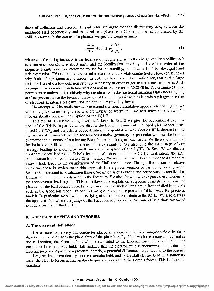
Let us consider a very flat conductor placed in a constant uniform magnetic field in the z direction perpendicular to the plane Oxy of the plate (see Fig. 1). If we force a constant current in the x direction, the electron fluid will be submitted to the Lorentz force perpendicular to the current and the magnetic field. Hall realized that the electron fluid is incompressible so that the Lorentz force must produce a pressure, namely, a potential difference perpendicular to the current.
Let j be the current density, 3 the magnetic field, and 8the Hall electric field. In a stationary state, the electric forces acting on the charges are opposite to the Lorentz forces. This leads to the equation
J. Math. Phys., Vol. 35, No. IO, October 1994
Downloaded 09 May 2005 to 128.32.113.135. Redistribution subject to AIP license or copyright, see http://jmp.aip.org/jmp/copyright.jsp
5376 Bellissard, van Elst, and Schulz-Baldes: Noncommutative geometry of quantum Hall effect
z
L!-
Y EM 1
M ++++++
c / t J > - - _ _ - - -
6
I
x
FIG. 1. The classical Hall effect: the sample is a thin metallic plate of width 8. The magnetic field .B is uniform and perpendicular to the plate. The current density j parallel to the x-axis is stationary. The magnetic field pushes the charges as indicated creating the electric field B along the y direction. The Hall voltage is measured between opposite sides along the y-axis.
nq2Y+jX.B=0, (2)
where n is the charge-carrier density and q is the charge of the carriers. Since the magnetic field .39 is perpendicular to both j and 8, solving (2) for j gives
where 97 is the modulus of the magnetic field and (+ is the conductivity tensor. The antidiagonal components of the tensor are the only nonvanishing ones and can be written as 2 crHS, where S is the plate width and oH is called the Hall conductance. Thus
We remark that the sign of oH depends upon the sign of the carrier charge. In particular, the orientation of the Hall field will change when passing from electrons to holes. Both possibilities were already observed by Hall using various metals. This observation is commonly used nowa- days to determine which kind of particles carries the current.
Let t” be the plate width in the y direction (see Fig. 1). The current intensity inside the plate is then given by Z=jS/ where j is the modulus of j. The potential difference created by the Hall field is V,= -&‘g.f’.u if u is the unit vector along the y axis. Using (2) we find
. .
In particular, for a given current intensity I, the thinner the plate the higher the potential differ- ence. For example, for a good conductor like gold at room temperature, the charge carrier density is of order of 6 X lO*‘m - 3 (see Ref. 18, Chap. 1). Thus, for a magnetic field of 1 T, a current intensity of 1 A and a potential difference of 1 mV the plate width is about 1 pm. These numbers
J. Math. Phys., Vol. 35, No. 10, October 1994
Downloaded 09 May 2005 to 128.32.113.135. Redistribution subject to AIP license or copyright, see http://jmp.aip.org/jmp/copyright.jsp
Bellissard, van Elst, and Schulz-Baldes: Noncommutative geometry of quantum Hall effect 5377
V
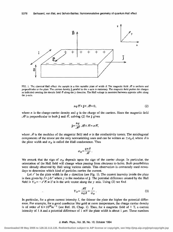
FIG. 2. Schematic representation of the experimental observations in the 1QI-E. The Hall conductivity CT” is drawn in units of e2/h vs filling factor Y. The dashed line shows the Hall conductivity of the Landau Hamiltonian without disorder. The direct conductivity q is shown in arbitrary units.
explain why the effect was so difficult to observe. It forced Hall to use very thin gold leaves in the beginning. In modern devices, much thinner “plates” with thickness of about 100 A are produced in inversion layers between two semiconductors.
In view of (3), the Hall conductance has the dimension of the inverse of a resistance. Since the product nc7 is the number of charge carriers per unit area, the dimensionless ratio
n6h v=-, .9e
called the$Zling factor, represents the fraction of a Landau level filled by conduction electrons of the thin plate. In terms of this parameter, we obtain for a free electron gas:
V h flH=-,
RH RH=T~
where RH is called the Hall resistance. It is a universal constant with value RH=25 812.80 Ct. RH can be measured directly with an accuracy better than 10e8 in QHE experiments. Since January 1990, this is the new standard of resistance at the national bureau of standards.3
B. The quantum Hall effect
Let us concentrate upon the dependence of the Hall conductance (in units of e*/h) on the filling factor v. In the classical Hall effect, these two quantities are just equal [Eq. (4)]. Lowering the temperature below 1 K leads to the observation of plateaux for integer values of the Hall conductance (see Fig. 2). In von Klitzing’s experiment,* the variation of v was obtained by changing the charge carrier density, whereas in later experiments one preferred varying the mag- netic field. The accuracy of the Hall conductance on the plateaux is better than 10e8. For values of the filling factor corresponding to the plateaux, the direct conductivity uII, namely the con- ductivity along the current density axis, vanishes. These two observations are actually the most important ones. The main problems to be explained are the following:
J. Math. Phys., Vol. 35, No. 10, October 1994 Downloaded 09 May 2005 to 128.32.113.135. Redistribution subject to AIP license or copyright, see http://jmp.aip.org/jmp/copyright.jsp

6)
(ii)
(iii)
(iv)
5378 Bellissard, van Elst, and Schulz-Baldes: Noncommutative geometry of quantum Hall effect
6) Why do the plateaux appear exactly at integer values? (ii) How do the plateaux appear? (iii) Why are these plateaux related to the vanishing of the direct conductivity?
To observe the QHE, physicists have used conduction electrons trapped in the vicinity of an interface between two semiconductors. The local potential difference between the two sides pro- duces a bending of the local Fermi level. Near the interface, this Fermi level meets with the valence band creating states liable to participate in the conductivity. This bending occurs on a distance of the order of 100 8, from the interface, so that the charge carriers are effectively concentrated within such a thin strip. In addition, by changing the potential difference between the two sides, the so-called gate voltage, one can control the charge-carrier density.
The samples used in QHE experiments belong to two different categories. The first one is called MOSFET,19 for metal-oxide silicon field effect transistors. The interface separates doped silicon from silicon oxide. This device was common in the beginning of the eighties and was the one used in von Klitzing’s experiment. However, the electron mobility is relatively low because the control of the flatness of the interface is difficult.
The samples of the other category are heterojunctions. The interface separates GaAs from an alloy of Al,Ga,-,As. This kind of device nowadays makes available interfaces almost without any defects. Moreover, electrons therein have a high mobility. These devices are most commonly used in modem quantum Hall experiments.
In both kinds of samples, there are many sources of defects producing microscopic disorder. The first comes from the doping ions. Even though they are usually far from the interface (about 1000 A), the long range Coulomb potential they produce is strong enough to influence the charges on the interface. It is not possible to control the position of these ions in the crystal. The second source of defects is the roughness of the interface. This is an important effect in MOSFET’s, much less in heterojunctions. In the latter the accuracy is better than one atomic layer in every 1000 8, along the interface.*’ Finally, long range density modulation of the compounds may produce visible effects. This is the case especially for heterojunctions where the aluminium concentration may vary by a few percent on a scale of 1 ,um.*l
It is important to notice that the observation of plateaux supposes several conditions.
The effect is more easily seen if the electron fluid is concentrated in such a thin region that it can be considered as two-dimensional. In fact, owing to the trapping effect of the poten- tial interface, the motion perpendicular to the interface is quantized. For good samples in high magnetic fields, the energy difference between two corresponding eigenvalues is big compared to kBT (where T is the temperature and kB the Boltzmann constant), so that only the lowest such level has to be considered. Hence the problem becomes effectively two- dimensional The plateaux disappear beyond a temperature of a few Kelvin. More exact, the inelastic relaxation time has to be large enough; otherwise corrections will be needed in formulas calculating the current; this will lead to the destruction of the plateaux. This is the reason why the IQHE is seen more easily in heterojunctions than in MOSFETs: the electron mobility in the former is higher than in the latter. We will see that some quenched disorder producing only elastic scattering is necessary for the appearance of the plateaux (see Sec. II D). In practice, the disorder that occurs is strong enough to produce a filling of the gaps between Landau levels.*t*‘* Clearly the sample size must be big enough as to allow the use of the infinite volume limit. Mesoscopic systems exhibit conductance fluctuations from sample to sample which may partially distroy the effect. Finite volume effects however have been shown to decrease exponentially fast with the sample size.
J. Math. Phys., Vol. 35, No. IO, October 1994
Downloaded 09 May 2005 to 128.32.113.135. Redistribution subject to AIP license or copyright, see http://jmp.aip.org/jmp/copyright.jsp

Bellissard, van Elst, and Schulz-Baldes: Noncommutative geometry of quantum Hall effect 5379
(v) Finally, the electric field needed to produce the current has to be small. If it is tod high, nonlinear phenomena may distroy the plateaux.23
Provided the previous conditions are satisfied, the quantum Hall effect is a universal phenom- enon. It is quite independent of the specific shape of the sample. Hall plateaux have also been observed in microwave experiments where the topology of the sample is trivial.24 Note, however, that the centers of the plateaux need not be located near integer values of the filling factor. It depends upon which kind of doping ion is used.2s The values of the Hall conductance, however, on the plateaux are independent of the nature of the used sample.
C. The Hall effect for the free Fermi gas
Let us first consider a very simple model in which the charge carriers are spinless, free, two-dimensional fermions with charge q. Our aim is to show that no quantization of the Hall conductance is observed in this case.
Since the particles are independent, the quantum motion is described by the one-particle Hamiltonian. Let A=(AI ,A2) be the vector potential given by
where 3’ is the modulus of the magnetic field. The energy operator is then given by the Landau Hamiltonian
H =(P-qN2 L 2m* ’
where P is the 2D momentum operator and m* is the effective mass of the particle. This operator is not translation invariant owing to the symmetry breaking produced by the vector potential. However, if one replaces the usual representation of the translation group by the so-called mag- netic translati*ns,27 the Landau Hamiltonian becomes translation invariant. Let us introduce the quasimomentum operators K= (P- qA)lh; they fulfill the canonical commutation relations
[Kl,K2]=r F.
Here q-8/h plays the role of an effective Planck constant. We see that the Landau Hamiltonian describes a harmonic oscillator so that its spectrum is given by the Landau levels, namely,
E,=fiw,(n+$),
where o, = q3’fm* is the cyclotron frequency and n E N. Each Landau level is infinitely degen- erate owing to translation invariance. The degeneracy per unit area is finite however and given by q2?/h. Perturbing this operator will give rise to a band spectrum.
Let us now compute the current. We assume the system to be in a thermodynamical equilib- rium. In order to allow nonzero current, we describe the system in the grand-canonical ensemble; in practice such a fluid is open. Since the particles are independent fermions, the thermal averaged density per unit volume of a one-particle translation invariant extensive observable @ at tempera- ture T and chemical potential p is given by
(@>I-+= lim -!- Tr~(f~,,Wd@ 1, AtR’ 1’1
J. Math. Phys., Vol. 35, No. 10, October 1994 Downloaded 09 May 2005 to 128.32.113.135. Redistribution subject to AIP license or copyright, see http://jmp.aip.org/jmp/copyright.jsp

5380 Bellissard, van Elst, and Schulz-Baldes: Noncommutative geometry of quantum Hall effect
wher: fT,I.l( E) = ( 1 + ePCE-p*)) - ’ is the Fermi-distribution function and p= l/kBT. In the limit above, A denotes a square box centered at the origin, and IAl is its area. The current is represented by the operator
J=+L ,X1,
where X is the position operator. It is easy to check that this current operator commutes with the magnetic translations. Obviously the thermal average of the current vanishes since no current can flow without an external source of energy. To make it nonzero, we switch on an electric field 8at time t = 0. For simplicity, we assume this field to be uniform and time-independent. After the field has been switched on, the time evolution is given by
~=+,,li,Jl, with HL,pH~--q&‘X.
The solution of this equation is elementary. Using complexified variables, that is M= M, + zM2 whenever M= (M, ,M2) is a 2D vector, we find
J(t)= -rq ~+eptmcfJO ,
where Jo is some initial datum. This solution consists of a time-independent part and of an oscillating part with the cyclotron frequency. The time average is just the constant part; it is the system’s response to the applied electric field. Taking the thermal average of this constant part, we have the observed current, namely, if j = j, + zj, ,
f ds j= lim
t-+m s o -$J(s))~,~=-I g:;Z h TrACfr,,(Ht))=-rqn $.
This is nothing but the classical formula (2), written in complex notation. Therefore we see that the classical Hall formula still holds in quantum mechanics for the free
fermion gas at all temperatures. There is no way to see any trace of quantization of the Hall conductance, neither is there any kind of plateaux of the Hall conductance!
D. The de of localization
The main experimental property we have not yet considered is the vanishing of the direct conductivity when the filling factor corresponds to the plateaux. In the previous argument we ignored all effects leading to a finite nonzero direct conductivity. Among these effects there are several sources of dissipation such as phonon scattering or photoemission. At very low tempera- ture, these sources usually have very limited influence and impurity scattering dominates. This is why we are led to consider nondissipative effects like Anderson localization in disordered systems. As explained in Sec. II B, several kinds of defects can influence the electron motion. These defects are usually distributed in a random way so that the forces they create on the charge carriers are actually represented by a random potential. In many cases one considers these defects as isolated and of small influence, so that a first-order perturbation theory based upon one-electron scattering on one impurity already gives a good account of the observed effects. For 2D systems however, it turns out that the low-density limit for impurities does not give the relevant contribution. We will see in Sec. III E how to define properly a potential representing the effects of a high density of random scatterers. For the moment let us stay at an intuitive level.
J. Math. Phys., Vol. 35, No. 10, October 1994
Downloaded 09 May 2005 to 128.32.113.135. Redistribution subject to AIP license or copyright, see http://jmp.aip.org/jmp/copyright.jsp

Bellissard, van Elst, and Schulz-Baldes: Noncommutative geometry of quantum Hall effect 5381
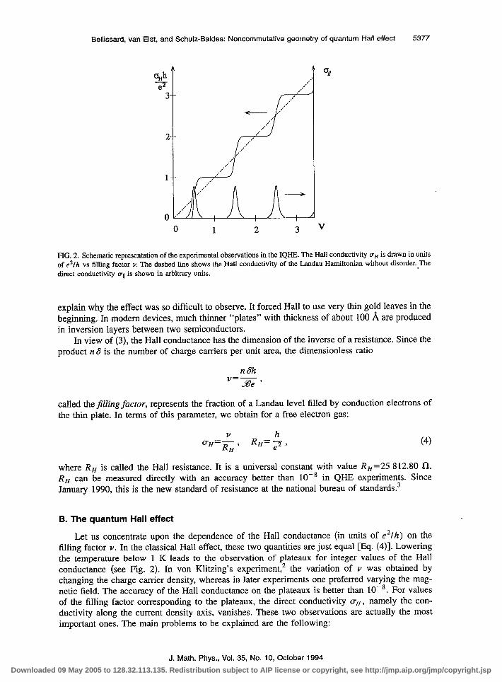
FIG. 3. The density of states for the Landau Hamiltonian with a random potential.
As explained by Anderson,2a the occurrence of a random potential in a one-particle Hamil- tonian may lead to the quantum localization of particles. More precisely, the quanta1 wave repre- senting these particles reflects on the potential bumps producing interferences. The Bragg condi- tion is necessary for building a constructive interference pattern throughout the crystal. This requires some regularity of the crystal, such as periodicity or quasiperiodicity, in order to allow the wave to propagate. If the potential creating these bumps exhibits some randomness, the probability for the Bragg condition to be satisfied everywhere in the crystal eventually vanishes. Therefore, the wave function will vanish at infinity leading to the trapping of particles in the local minima of the potential. This is Anderson localization.
It has been argued29 that one-dimensional systems of noninteracting particles in a disordered potential exhibit localization at any strength of disorder. Mathematicians have proved such a claim under relatively mild conditions on the randomness of the potentia1.30-34 They have also proved localization in any dimension for strong disorder.3s-40 A finite-size scaling argument, proposed by Thouless, has been used in Ref. 29 to show that two-dimensional systems are also localized at any disorder unless there are spin-orbit couplings.42 The same argument also shows that in higher dimensions, localization disappears at low disorder. We remark that the notion of localization we are using does not exclude divergence of the localization length at an isolated energy. These results were supplemented by many numerical calculations.43-46
On the other hand, the occurrence of a random potential will create new states with energies in the gaps between Landau levels. This can be measured by the density of states (DOS). To define it, let .k’TE) be the integrated density of states (IDS), namely, the number of eigenstates of the Hamiltonian per unit volume below the energy E:
Jt’T E) = lim -!- # {eigenvalues of HI A-rm IAl A-), (6)
where degenerate eigenvalues are counted with their multiplicity. This is a nondecreasing function of E. Therefore its derivative p(E) =dM(E)ldE is well defined as a Stieljes-Lebesgue positive measure and is called the DOS. Under mild conditions on the distribution of the random potential, it is possible to show47*34,33 that the DOS is a smooth function (see Fig. 3). If the potential strength exceeds the energy difference fLw, between two consecutive Landau levels, the gaps will be entirely filled. This is actually the physical situation in most samples used up to now. In hetero- junctions, for instance, the minimum of the density of states may represent as much as 30% of its maximum,‘l although in modem samples it is usually very smal1.22
Recall that the chemical potential at zero temperature is called the Fermi Zevel EF . Since the charge carriers are spinless fermions, their density at T=O is given by
J. Math. Phys., Vol. 35, No. 10, October 1994 Downloaded 09 May 2005 to 128.32.113.135. Redistribution subject to AIP license or copyright, see http://jmp.aip.org/jmp/copyright.jsp
5382 Bellissard, van Elst, and Schulz-Baldes: Noncommutative geometry of quantum Hall effect
I EF n= dE p(E)=M(E,). (7) -co
The absence of spectral gaps means that the IDS is monotone increasing, so that changing con- tinuously the particle density is equivalent to changing continuously the Fermi level. More gen- erally, if a magnetic field is switched on, changing continuously the filling factor is equivalent to changing continuously the Fermi level. On the other hand, while the Fermi level crosses a region of localized states, the direct conductivity must vanish whereas the Hall conductivity cannot change since localized states do not participate to the current. This last fact is not immediately obvious, but more justification will be given later on. Changing the filling factor therefore will force the Fermi level to change continuously within this region of localized states while the Hall conductance will stay constant. This is the main mechanism leading to the existence of plateaux.
In contrast, if the spectrum had no localized states, the Hall conductance would change while changing the filling factor, as long as the Fermi level would move within the spectrum. Moreover, if a spectral gap occurred between two bands, let us say between energies E- and E, , the IDS would equal a constant no on that gap and changing the filling factor from no- E to no+ E would cause the Fermi level to jump discontinuously from E- to E, with the value (E- +E+)/2 whenever n = n o. In this case, once again, no plateaux could be observed. This is why there is no quantized Hall effect in the free fermion theory.
One of the consequences of this argument is that between two different plateaux, there must be an energy for which the localization length diverges.5’P13 Even though there should be no extended states in 2D disordered systems, the localization length need not be constant in energy. As it happens, if the impurities are electrically neutral in the average, the localization length diverges exactly at the Landau levels. Therefore, the influence of impurities decreases near the band centers, and other sources of interactions, like the Coulomb potential between charge carri- ers, may become dominant. This is actually the basic observation leading to the understanding of the FQHE.
We have argued that the direct conductivity should vanish whenever the Fermi level lies in a region of localized states. One may wonder how it is then possible to have a nonzero Hall conductance. The answer is that the Hall current is actually carried by edge states. This has been seen in numerical calculations48*49 and there are the first theoretical hints.50 The experimental situation is not as clear as it looks from theory. This is probably due to the existence of zones in which states are localized surrounded by filamentary regions in which the Hall current can actually flow.“7
E. The Laughlin argument
The first attempt to explain the integer quantization of the Hall conductance in units of e2/h was proposed by Laughlin.’ Laughlin originally chose a cylinder geometry for his argument. His justification for this was that the effect seemed to be universal and should therefore be independent of the choice of the geometry. Here, we present a Laughlin argument in the plane in form of a singular gauge transformation. In Sec. IV H, this presentation and an observation of Avron, Seiler, and Simon” will allow us to discuss the links between the Laughlin argument and the Chem-character approach presented in this article.
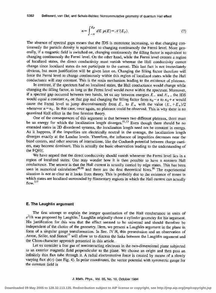
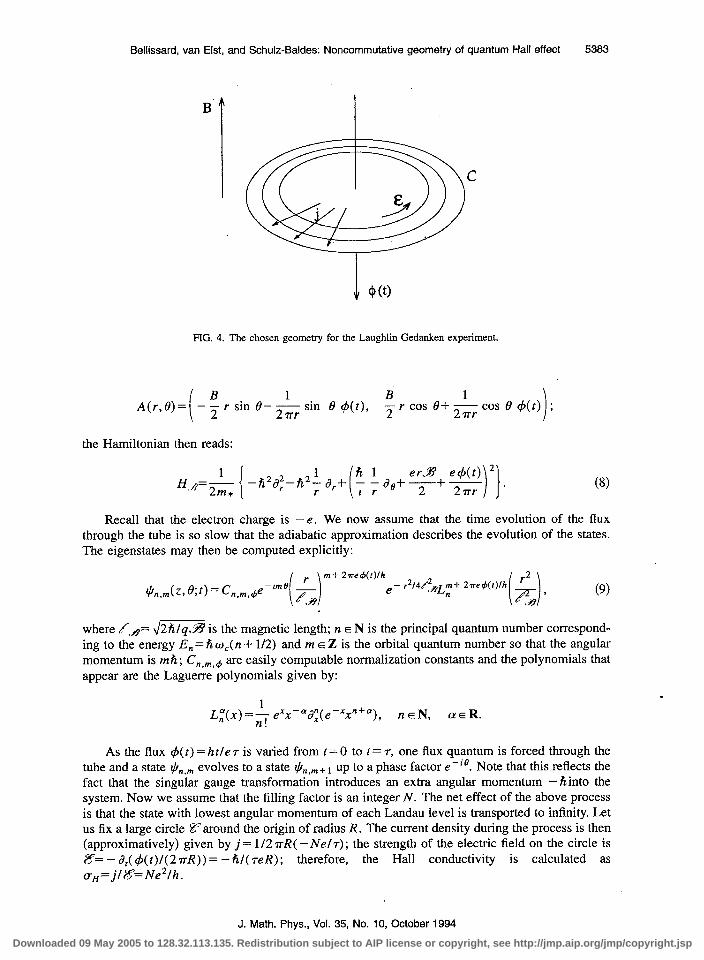
Let us consider a free gas of noninteracting electrons in the two-dimensional plane subjected to an exterior magnetic field perpendicular to the plane. We choose an origin and then pass an infinitely thin flux tube through it. A radial electromotive force is created by means of a slowly varying flux 4(t) (see Fig. 4). In polar coordinates, the vector potential with symmetric gauge for the constant field is
J. Math. Phys., Vol. 35, No. 10, October 1994
Downloaded 09 May 2005 to 128.32.113.135. Redistribution subject to AIP license or copyright, see http://jmp.aip.org/jmp/copyright.jsp
Bellissard, van Elst, and Schulz-Baldes: Noncommutative geometry of quantum Hall effect 5383
FIG. 4. The chosen geometry for the Laughlin Gedanken experiment.
B -Grsin8--&sin /3&t), ~rcosB+
the Hamiltonian then reads:
1 H,fl=-
2m* 1
er37 e+(t) 2 -Ii2+fi2; e,+ ; ; a,+ 2+ -
i 11 27rr *
Recall that the electron charge is - e. We now assume that the time evolution of the flux through the tube is so slow that the adiabatic approximation describes the evolution of the states. The eigenstates may then be computed explicitly:
m+ 2mqt(r)lh
e- r=14e~~y+ 2m$(tVh
n (9)
where /.A= ~/m is the magnetic length; n E N is the principal quantum number correspond- ing to the energy E, = h o,( n + l/2) and m E Z is the orbital quantum number so that the angular momentum is mh; C,,,.4 are easily computable normalization constants and the polynomials that appear are the Laguerre polynomials given by:
1 L:(X)=; exx-ad~(e-xxn+a), n EN, CYER.
As the flux 4(t) = htle T is varied from t = 0 to t = T, one flux quantum is forced through the tube and a state ICI,,,, evolves to a state I/$,~+ t up to a phase factor eCie. Note that this reflects the fact that the singular gauge transformation introduces an extra angular momentum -Tiinto the system. Now we assume that the filling factor is an integer N. The net effect of the above process is that the state with lowest angular momentum of each Landau level is transported to infinity. Let us fix a large circle Fararound the origin of radius R. The current density during the process is then (approximatively) given by j= 1/2~R( - Ne/T); the strength of the electric field on the circle is ;;f?= - a,( +( t)l( 2 vR)) = - fLl( TeR); therefore, the Hall conductivity is calculated as aH=j18=Ne21h.
J. Math. Phys., Vol. 35, No. IO, October 1994
Downloaded 09 May 2005 to 128.32.113.135. Redistribution subject to AIP license or copyright, see http://jmp.aip.org/jmp/copyright.jsp
5384 Bellissard, van Elst, and Schulz-Baldes: Noncommutative geometry of quantum Hall effect
What did we learn from this argument? Until now, not so much in fact. For had we taken another noninteger filling factor v and supposed that the electron density were uniform, we would obtain oH= ve2/h; that is the classical result already calculated in Sec. II D.
Using ideas of Prange, Halperin, and Joynt9*‘0s51 however, the picture may be completed to furnish a qualitative understanding of the IQHE in the following way: if the sample has impurities, these transform some of the extended states (9) into localized states; moreover, the explicit form of the remaining extended states changes. Now the localized states will not change as a flux quantum is forced through the flux tube, and it can be argued that the remaining extended states of one Landau level still carry the same current, that is one charge e through the circle V. As some of the localized states caused by the impurities are situated below the energy of the Landau levels and others above, we come to the desired qualitative explanation with help of the argument explained in Sec. II D.
There are two ingredients in this Gedanken-experiment which ought to be emphasized. The first is the gauge invariance which produces the periodicity of the Hamiltonian with respect to the varying flux, the period being the flux quantum. The second is that the Hall effect corresponds to a charge transport of one unit for each filled Landau level. The conductance quantization is therefore likely to be connected to the charge quantization.
F. The Chern-Kubo relationship
The geometrical origin of the Hall conductance quantization was revealed by TKN2 (Ref. 8) and Avron et al. l2 TKN2 considered an electron gas submitted to a uniform magnetic field on a 2D square lattice in the tight-binding approximation. In the Landau gauge the Hamiltonian reads
(ff$)(m~md=$l(m~- l,md+ #(ml+ l,mz)
+e-2”am1+(m1,m2- l)+e2r~m~~(m1,m2+ l), (10)
where CY= q5/bo is the ratio of the magnetic flux C$ in the unit cell to the flux quantum c$~ = h/e. Using the translation invariance along the y axis, the solution of the eigenvalue equation can be written in the form
q(m,-l)+p(ml+l)+2 cos(k2-27nxml)q(ml)=E(k2)cp(ml). (11)
This is Harper’s equation.52 It can also be obtained by adding a weak periodic potential to the Landau Hamiltonian (5) and then projecting onto one Landau level. Now TKN, assumed that the ratio (Y is a rational number of the form p/q where p and q are relatively prime integers. By translation invariance of period q, the solution of Eq. (11) can also be written in Bloch’s form
so that Harper’s equation now becomes
J. Math. Phys., Vol. 35, No. IO, October 1994
Downloaded 09 May 2005 to 128.32.113.135. Redistribution subject to AIP license or copyright, see http://jmp.aip.org/jmp/copyright.jsp

Bellissard, van Elst, and Schulz-Baldes: Noncommutative geometry of quantum Hall effect 5385
This is the secular equation for the q X q Hermitian matrix H(kl ,k2). The energy spectrum is given by energy bands corresponding to the eigenvalues EI( k 1 , k,) , 1 G 1 G q . Let P,( k 1 , k2) be the corresponding eigenprojection. We will assume for simplicity that all bands are well separated: for the Harper equation, all gaps but the central one are open.‘3-55
It is quite clear that H(kl ,k2) is a trigonometric polynomial in (k, ,k2), implying that the eigenprojections and the eigenvalues are smooth periodic functions of (k, ,k2). Moreover, intro- ducing the two unitary qXq matrices defined by
we derive the covariance relation
(12)
These relations show that the eigenvalues and the trace of any function of H and its derivatives are actually 2 r/q-periodic in (k, , k,) .
The Hall conductance can now be calculated by Kubo’s formula.56 It gives the current as the velocity-velocity correlation function. The formula may be deduced from classical arguments using the Boltzmann equation,56 but a deduction closer to quantum mechanics using linear re- sponse theory will be presented in Sec. IV. The result derived by TKN2 is then the following: at zero temperature, if the Fermi level belongs to a gap of the Harper Hamiltonian of Eq. (lo), the transverse conductivity is given by the Kubo-Chem relation (see Ref. 12)
e2 uH=7;- WP,),
where
Ch( PF) = (13)
Here d, = dldk, , a = 1, 2, and P, is the eigenprojection on energies smaller than the Fermi level. The integrand is a complex 2-form on the torus; its de Rham-cohomology class is called the first Chem class or the first Chem character of the projection P, . We shall also refer to the integral over this form as Chem character, because the integral will retain meaning in the noncommutative context; the integral will also be called Chem number.
For further informations on Chem classes and characters we refer to Refs. 57 and 58. The Chem character of a projection is a topological invariant. To see this, we remark that the data of the family k = (k 1 ,k2) E T2* PF( k) of projections defines a complex fiber bundle 9’F over the 2-torus in a natural way. More precisely, 9’F is the set of pairs (k,t) E T2X C4 such that P,(k)t= 5. Since the Fermi level lies in a gap, PF is smooth and its dimension is constant. Therefore .Y’F is a smooth vector bundle over the 2-torus. It can be shown that Ch( PF) depends only upon the equivalence class of 9F provided the equivalence is isomorphism of vector bundles modulo adding trivial bundles. In particular, it is a homotopy invariant quantity. This implies that adding a small perturbation to the Harper Hamiltonian will not change the value of Ch( PF), at least as long as the Fermi level does not cross the spectrum while turning on the perturbation! This is the argument that was needed to explain the robustness of the Hall conductance.
In addition to being robust, the Chem number Ch(PF) is actually an integer. To see this explicitly, we will show (see Sec. IV E) that the Chem character Ch is additive with respect to the direct sum of two orthogonal projections P and Q, that is Ch( P CD Q) = Ch( P) + Ch( Q). Even
J. Math. Phys., Vol. 3.5, No. 10, October 1994
Downloaded 09 May 2005 to 128.32.113.135. Redistribution subject to AIP license or copyright, see http://jmp.aip.org/jmp/copyright.jsp

5386 Bellissard, van Elst, and Schulz-Baldes: Noncommutative geometty of quantum Hall effect
though this is not obvious from Eq. (13), all cross-terms in the left hand side vanish. It is thus sufficient to show that if P is a one dimensional smooth projection over T*, then its Chem character is an integer. This can be shown as follows.
Let e(k) be a unit vector in the vector space C4 such that P(k)&k) = e(k), Vk. It is easy to show that
Ch(p)=Jr2 2 Tr(P(k)[a,P(k),a,P(k)])=~~~*~dk,~~~dk23m(a,5(k)ld25(k)),
(14)
where 3m is the imaginary part. Using Stokes formula, this double integral can be written as
Ch(P)=
Even though P is doubly periodic in k, 5 need not be periodic. The obstruction to the periodicity of 5 is precisely the nonvanishing of the Chem character. However, we can find two real functions 8i and e2 such that
5(k1,2r)=e “1(~1)&k1,0), ~(2m,k2)=e’ez(‘2)~(0,k2), (16)
provided O~kt~2rr and 0~ k2=S2r, respectively. The reason is that after one period the new vector 5 defines the same subspace as the old one, so they are proportional. Since E(k) is a unit vector for any k, the proportionality factor must be a phase. Writing 5( 2 7r,27r) in two ways we get 6t(2rr)- e,(O)= 8,(2a)- e,(O) (mod 2779. Replacing in Eq. (15) leads to
,,(,)=(e,(2~)-e,(o))-(e2(2~)-e2(0)) EZ 2rr
Thanks to this argument, we see that the Chem character of a smooth projection valued function over the 2-torus is an integer.
We remark, however, that the expression used in Eq. (14) is not exactly the same as the one used in Eq. (13): in the latter, we have divided by q. However, the covariance relation Eq. (12) shows that the integrand in Eq. (13) is 2 r/q-periodic in k so that it is sufficient to integrate over the square [0,2dq]‘* and multiply the result by q*. On the other hand, the periodicity condition (16) has to be modified to take the covariance into account. Now the argument goes along the same line and gives rise to an integer as well.
This series of arguments shows that indeed the Hall conductance (in units of e*/h) is a very robust integer, as long as the Fermi level remains in a spectral gap. However, the previous argument does not work for any kind of perturbation. It is valid provided the perturbation of the Hamiltonian is given by a matrix valued function &f(k) satisfying the same covariance condition (12). Otherwise, the previous construction does not tell us anything about the homotopy invariance of the Hall conductance. This is exactly the limitation of the TKN2 result. More precisely, no disorder is allowed here and, in addition, only a rational magnetic field can be treated in this way, a quite unphysical constraint. For indeed, in most experiments the variation of the filling factor is obtained through changing continuously the magnetic field. Even though rational numbers are dense in the real line, the previous expression (13) depends in an explicit way on the denominator q of the fraction so that we have no way to check whether the integer obtained is robust when the magnetic field is changed.
The drastic condition of having no disorder is also disastrous: the periodicity of the Hamil- tonian excludes localized states, and the argument in Sec. II D shows that no plateaux can be observed in this case. Therefore we have not yet reached the goal.
J. Math. Phys., Vol. 35, No. 10, October 1994
Downloaded 09 May 2005 to 128.32.113.135. Redistribution subject to AIP license or copyright, see http://jmp.aip.org/jmp/copyright.jsp

Bellissard, van Elst, and Schulz-Baldes: Noncommutative geometry of quantum Hall effect 5387
Nevertheless, the main result of TKN, is the recognition that the Hall conductance can be interpreted as a Chem character. This is a key fact in understanding why it is quantized and robust as well. Moreover, the topology underlying this Chem character is that of the quasimomentum space, namely, the periodic Brillouin zone which is a 2-torus. From this point of view, the Laugh- lin argument in its original form may be misleading since it gives the impression of emphasizing the topology of the sample in real space, which has nothing to do with the IQHE.
The solution to the TKN2 limitation is given by the noncommutative geometry of the Bril- louin zone where both of the above restrictions can be dropped. We will see that the Kubo-Chem relation still holds, that the Chem character is still a topological invariant and that it is an integer. But we will also discover something new, characteristic of noncommutative geometry, namely, that localization can be expressed in a very clear way in this context and that the conclusion will be valid as long as the Fermi level lies in a region of localized states.
III. THE NONCOMMUTATIVE GEOMETRY OF THE IQHE: THE FOUR-TRACES WAY
In this section the strategy and the main steps of the noncommutative approach are given. In particular we will introduce the four different traces that are technically needed to express the complete results of this theory. The first one is the usual trace on matrices or on trace-class operators. The second one, introduced in the Sec. III A below, is the trace per unit volume which permits to compute the Hall conductance by the Kubo formula. The third one is the graded truce or supertrace introduced in Sec. III B. This is the first technical tool proposed by Connes4 to define the cyclic cohomology and constitutes the first important step in proving quantization of the Hall conductance.i6 The last one is the Dixmier truce defined by Dixmier in 196459 and of which the importance for quantum differential calculus was emphasized by Connes.60’5.6 It will be de- fined in Sec. IV D but we already explain in Sec. III C below how to use it in order to relate localization properties to the validity of the previous results.
A. The noncommutative Brillouin zone
In a D-dimensional perfect crystal, the description of observables is provided by Bloch’s theory. Owing to the existence of a translation group symmetry, each observable of interest commutes with this group. It is a standard result in solid state physics that such an observable is a matrix valued periodic function of the quasimomenta k. The matrix indices usually label both the energy bands and the ions in the unit cell of the crystal whenever it is not a Bravais lattice. The period group in the quasimomentum space is the reciprocal lattice.
If the crystal suffers disorder or if a magnetic field is turned on, this description fails. In most situations however, physicists have found ways to overcome this difficulty. For instance, impuri- ties are treated as isolated objects interacting with the electron Fermi sea using perturbation theory. Magnetic fields in 3-dimensional real crystals are usually so small that a quasiclassical approxi- mation gives a very good account of the physical properties.
Still the conceptual problem of dealing with the breaking of translation symmetry remains. It has not been considered seriously until new physical results forced physicists to face it. One important example in the past was Anderson localization due to a random potentia1.28,29’33*32-34 Even though important progress has been made, the solution is still in a rather rough shape and numerical results are still the only justification of many intuitive ideas in this field. When arriving at the QHE, the role of localization became so important that there was no way to avoid it.
The main difficulty in such cases is that translates of the one-electron Hamiltonian no longer commute with the Hamiltonian itself. Nevertheless, the crystal under study is still macroscopically homogeneous in space so that its electronic properties are translation invariant. Thus choosing one among the translates of the Hamiltonian is completely arbitrary. In other words, the one-electron Hamiltonian is only known up to translation. Our first proposal to deal with this arbitrariness is to
J. Math. Phys., Vol. 35, No. 10, October 1994
Downloaded 09 May 2005 to 128.32.113.135. Redistribution subject to AIP license or copyright, see http://jmp.aip.org/jmp/copyright.jsp
5388 Bellissard, van Elst, and Schulz-Baldes: Noncommutative geometry of quantum Hall effect
consider all the translates at once. More precisely, our basic object is the observable algebra ./% generated by the family of all translates of the one-electron Hamiltonian in the space G, where G is either RD or ZD.
It is remarkable that the algebra ~6 exists in the periodic case as well and coincides then with the algebra of matrix-valued, periodic, continuous functions of the quasimomenta. In this case, due to the periodicity with respect to the reciprocal lattice, it is sufficient to consider quasimo- menta in the first Brillouin zone B. Then B is topologically a D-dimensional torus. Therefore the matrix elements of a typical observable are continuous functions over B.
Proceeding by analogy, we will consider the algebra ~6 in the nonperiodic case as the non- commutative analog of the set of continuous functions over a virtual object called the “noncom- mutative Brillouin zone.” ‘4&l This is, however, ineffective as long as we have not defined rules for calculus. In the periodic case physical formulas require two kinds of calculus operations, namely, integrating over the Brillouin zone and differentiating with respect to quasimomenta.
If A is an observable in a periodic crystal, its average over quasimomenta is given by
(A)= fB$ ‘WA(k)).
Here IBI represents the volume of the Brillouin zone in momentum space. It turns out that such an average coincides exactly with the “trace per unit volume,” namely, we have
where A is a square centered at the origin, IAl is its volume, Tr* and A* are the restrictions of the trace and the observable A respectively to A.
In a nonperiodic, but homogeneous crystal it is still possible to define the trace per unit volume T(A) of an observable A. Formula (17) however becomes ambiguous in this case, be- cause the limit need not exist. We will show in Sec. III F how to define Yin general. It will satisfy the following properties:
(i) Y-is linear, like the integral; (ii) Yis positive, namely, if A is a positive observable, Y(A) 30; (iii) .Yis a trace, namely, even though observables may not commute with each other, we still
have Y(AB)=F(BA).
Differentiating with respect to quasimomenta can be defined along the same line. In the periodic case, we remark that the derivative djA = dAldkj is also given by
ajA=-z[Xj, A], (18)
where X=(X i ,...,X& is the position operator. We will use the formula (18) as a definition of the derivative in the nonperiodic case. Owing to the properties of the the commutator it satisfies:
ii) a is linear. 4 obeys the Leibniz rule d.(AB)=(d.A)B+A(d.B)
(iii) dj commutes with the adjo/nt operatic&, namely, ij(A *) = ( EJjA)*.
Such a linear map on the observable algebra is called a “ * -derivation.” In our case it is moreover possible to exponentiate it, for, if 8= (8t , . . . . e,), we find
J. Math. Phys., Vol. 35, No. 10, October 1994
Downloaded 09 May 2005 to 128.32.113.135. Redistribution subject to AIP license or copyright, see http://jmp.aip.org/jmp/copyright.jsp

Bellissard, van Elst, and Schulz-Baldes: Noncommutative geometty of quantum Hall effect 5389
where 8.X= ( 6$X, + ---+8,x,) and e.v=(e,dl+ *a. + eDa,). Equipped with the trace per unit volume and with these rules for differentiations, .& becomes a “noncommutative manifold,” namely, the noncommutative Brillouin zone.
B. Hall conductance and noncommutative Chern character
Using the dictionary created in the previous section between the periodic crystals and the non-periodic ones and in view of Eq. (13), one is led to the following formula for the Hall conductance at zero temperature
uH=; Ch(PF), W’d=& flPd4PFrW’Fl)r (19)
where P, is the eigenprojection of the Hamiltonian on energies smaller than or equal to the Fermi level EF . We will justify this formula in Sec. IV B below within the framework of the relaxation time approximation. However this formula is only valid if
(9 the electron gas is two-dimensional (so D = 2); (ii) the temperature is zero; (iii) the thermodynamic limit is reached; (iv) the electric field is vanishingly small; (v) the collision time is infinite; (vi) electron-electron interactions are ignored.
We will discuss in Sec. IV C the various corrections to that formula whenever these conditions are not strictly satisfied.
The main result of this paper is that the noncommutative Chern character Ch(PF) of the Fermi projection is an integer provided the Fermi level belongs to a gap of extended states (see Theorem 1). Moreover, we will show that it is a continuousfunction of the Fermi level as long as this Zutter lies in a region of localized states (see Theorem 1). This last result implies that changing the filling factor creates plateaux corresponding to having the Fermi level in an interval of local- ized states (see proposition 14). In addition, whenever the Hall conductance jumps from one integer to another one, the localization length must diverge somewhere in between [see Corollary (311.
In order to get this result we will follow a strategy introduced by Connes in this context,4 but originally due to Atiyah.6* Before describing it, we need some notations and definitions. We build a new Hilbert space which is made of two copies .%+ and 9Y- of the physical Hilbert space .% of quantum states describing the electron. This is like working with Pauli spinors. In this doubled Hilbert space .%= %+ @ 9.Y- , the grading operator G and the “Hilbert transform” F are defined as follows:
(20)
where X=X, + zX2 (here the dimension is D = 2). It is clear that F is self-adjoint and satisfies F2= 1. An operator T on .% will said to be of degree 0 if it commutes with 6 and of degree 1 if it anticommutes with 6. Then, every operator on & can be written in a unique way as the sum T= TO+ T1 where Tj has degree j. The graded commutator (or supercommutator) of two operators and the graded differential dT are defined by
J. Math. Phys., Vol. 35, No. 10, October 1994
Downloaded 09 May 2005 to 128.32.113.135. Redistribution subject to AIP license or copyright, see http://jmp.aip.org/jmp/copyright.jsp
5390 Bellissard, van Elst, and Schulz-Baldes: Noncommutative geometry of quantum Hall effect
[T, T’ls=TT’-( -)deg(T)deg(T’)TrT, dT=[F, Tls.
Then, d*T=O. The graded trace Trs (or supertrace) is defined by I I
Trs(T)=i Tr,+(GF[F,T]s)=Tr,x(T++-uT--u), (21)
where u =Xl[X] and T + + and T-- are the diagonal components of T with respect to the decom- position of 3%‘. It is a linear map on the algebra of operators such that Tr,( TT’) = Trs( T’T). Moreover, operators of degree 1 have zero trace. However, this trace is not positive. Observables in . +3 will become operators of degree 0, namely, A E ~8 will be represented by i =A + @ A - where AZ acts as A on each of the components .3iYZ = .%‘.
With this formalism, Connes4 gave a formula which was extended to the present situation in Ref. 16 to the following one (see Sec. IV F):
Ch( PF) = I
odP( o)Trs( kFdP,d@,), (22)
where the space R represents the disorder configurations while the integral over dP is the average over the disorder. We will show that the integrand does not depend upon the disorder configura- tion. Moreover, we will show that the right hand side of (22) is P-almost surely equal to the index of a Fredholm operator, namely,
(23)
The Chem character is therefore an integer, at least whenever it is well-defined. One may wonder what is the physical meaning of this integer. Actually, an answer was
provided quite recently by Avron et a1.17 Considering the definition of the graded trace in formula (21), they interpreted the index found for the Chem character as the relative index of the projec- tions PF and UP+. This is to say even though these projections are infinite-dimensional, their difference has finite rank giving rise to a new index called the “relative index.” Then they argue that u represents the action of the singular Laughlin gauge (see Sec. II E) and that this difference can be interpreted as a charge transported to infinity as in the original Laughlin argument.7
C. Localization and plateaux of the Hall conductance
In Sec. III B, we have explained the topological aspect of the Hall conductance quantization. However, these formulas only hold if both sides are well defined. For instance, it is not clear whether the Fermi projection is differentiable. If it is not, what is the meaning of formula (19)? This is the aspect that we want to discuss now.
First of all, using the Schwarz inequality, a sufficient condition for formula (19) to hold is that the Fermi projection satisfy Y( 1 VP,/*) < a~ if we set V= (at ,a,). It is important to remark that this condition is much weaker than demanding P, to be differentiable. This is rather a noncom- mutative analog of a Sobolev norm (or the square of it). By definition, this expression can be written as
(24)
Note that Eq. (24) can be defined in any dimension D. From this expression, we see that the finiteness of the Sobolev norm is related to the finiteness of some localization length. Indeed, we will show that only the part of the energy spectrum near the Fermi level gives a contribution to formula (24) so that P, can be replaced by the projection PA onto energies in some interval A
J. Math. Phys., Vol. 35, No. 10, October 1994
Downloaded 09 May 2005 to 128.32.113.135. Redistribution subject to AIP license or copyright, see http://jmp.aip.org/jmp/copyright.jsp
Bellissard, van Elst, and Schulz-Baldes: Noncommutative geometry of quantum Hall effect 5391
close to EF. On the other hand, the matrix element (01 PA/x) gives a measure of how far states with energies in A are localized. Thus, the Sobolev norm is some measurement of the localization length. We will develop this fact in Sec. V B below. One way of defining a localization length consists in measuring how far a wave packet goes in time. This gives
12(A)=;ym T r=O ’ T dt ndPto)(OIItX(t)-X)1210), I J wherethe timeevolutionisgovemedbyHPa andwhere[Al*=X,A*A,ifA=(At,...,A,). Inthis expression, X is the position operator and X(t) is the evolution of X under the one-electron Hamiltonian after time r. Let now JQ” be the density of states (DOS) already introduced in Sec. II D. It can be defined equivalently as the positive measure Jy- on the real line such that for any interval A
That these two definitions coincide is guaranteed by a theorem of Shubin.61,63 We will show that if Z2(A) is finite, there is a positive H-integrable function Z(E) over A such that
l*(A’) = I A,d-‘WW)2,
for any Bore1 subset A’ of A (see Theorem 13). The number Z(E) will be called the “localization length” at energy E. Moreover, we also find
such that the mapping EF~ A I+ PF is continuous with respect to the Sobolev norm (Theorem 14).
The previous argument shows that, whenever the localization length at the Fermi level is finite, the Chem character of the Fermi projection is well defined. Now let us consider the right hand side of formula (22). In a recent work Connes60’5 proposed to use another trace which was introduced in the sixties by Dixmier.59 This Dixmier trace Trnix will be defined in Sec. IV D. Let us simply say that it is a positive trace on the set of compact operators, such that any trace-class operator is annihilated by it whereas if T is a positive operator with finite Dixmier trace, then T ’ +’ is trace class for any E>O. In Ref. 60, Connes proved a formula relating the so-called Wodzicky residue of a pseudodifferential operator to its Dixmier trace. Adapting this formula to our situation leads to the following remarkable result (see Theorem 9):
s(jVP,[*)=i Trn,(IdPF1*).
Note that this formula only holds for electrons in two dimensions. In higher dimensions, things are more involved. Therefore, we see that as soon as the localization length is finite in a neighborhood of the Fermi level, the operator dkF is square summable with respect to the Dixmier trace implying that its third power is trace-class. In view of the formulas (21) and (22), we see that this is exactly the condition for the existence of the right-hand side of Eq. (22). Moreover, the conti- nuity of PF in EF with respect to the Sobolev norm implies that the index in formula (23) is
J. Math. Phys., Vol. 35, No. 10, October 1994
Downloaded 09 May 2005 to 128.32.113.135. Redistribution subject to AIP license or copyright, see http://jmp.aip.org/jmp/copyright.jsp

5392 Bellissard, van Elst, and Schulz-Baldes: Noncommutative geometry of quantum Hall effect
constant as long as the Fermi level stays in a region in which the localization length is finite. Therefore the Chem character is an integer and the Hall conductance is quantized and exhibits plateaux.
In this way, the mathematical frame developed here gives rise to a complete mathematical description of the IQHE, within the approximations that have been described previously.
D. Summary of the main results
Let us summarize our mathematical results in this section.
Theorem 1: Let H=H* be a Hamiltonian affiliated to the C*-algebra .A=C*(OXG,$) defined in Sec. III F Let P be a G-invariant and ergodic probability measure on a. Then we have the following results:
(i) (Kubo-Chern formula) In the limit where (a) the volume of the sample is injinite, (b) the relaxation time is infinite, and (c) the temperature is zero,
the Hall conductance of an electron gas without interaction and described by the one-particle Hamiltonian H is given by the formula
on=; Ch(PF)=; 2z7rY7P,[d,P,,a2P,]),
where PF is the eigenprojection of H on energies smaller than or equal to the Fermi level EF and Tis the trace per unit volume associated to P.
(ii) (Quantization of the Hall conductance) Ifin addition P, belongs to the Sobolev space Y associated to .A, then Ch(P,) is an integer which represents the charge transported at infinity by a Laughlin adiabatic switching of a flux quantum.
(iii) (Localization regime) Under the same conditions as the ones in (ii), the direct conductivity vanishes.
(iv) (Existence of Plateaux) Moreover; if A is an interval on which the localization length l*(A) dejned in Sec. III C is jinite, then as long as the Fermi energy stays in A and is a continuity point of the density of states of H, CJh(Pr) is constant and Pr belongs to the Sobolev space 9?
The following corollary is an immediate consequence. It was proved in Refs. 51 and 13.
Corollary 1: If the Hall conductance au jumps from one integer to another in between the values v1 and v2 of theJilling factol; there is an energy between the corresponding values of the Fermi levels at which the localization length diverges.
Strictly speaking, this theorem has been completely proved only for the case of a discrete lattice (tight-binding representation). Most of it is valid for the continuum, but parts of the proofs require extra technical tools so that the proof of this theorem is not complete in this paper. We postpone the complete proof of it for the continuum case to a future work.@
As a side result, we emphasize that we have developed a noncommutative framework valid to justify the transport theory for aperiodic media (see Sec. IV A below). It allows us to give rigorous estimates on the error terms whenever the conditions of the previous theorem are not strictly satisfied (see Set IV C below). We will not give the mathematical proofs that these errors are
J. Math. Phys., Vol. 35, No. 10, October 1994
Downloaded 09 May 2005 to 128.32.113.135. Redistribution subject to AIP license or copyright, see http://jmp.aip.org/jmp/copyright.jsp

Beliissard, van Elst, and Schulz-Baldes: Noncommutative geometry of quantum Hall effect 5393
rigorous bounds here even though they actually are. This will also be the main topic of a future work. But we have estimated them and we show that they are compatible with the accuracy observed in the experiments.
Another result which is actually completely developed here due to its importance in the quantum Hall effect, concerns the definition and the properties of the localization length. We give a noncommutative expression for it and show how it is related to the existence of plateaux. The main results in this direction are the Theorems 13 and 14 in Sec. V B. We also show that the localization length is indeed finite in models like the Anderson model for disordered systems for which proofs of exponential localizations are available.
The proof of Theorem I will be divided up into a number of partial results; there will be no explicit paragraph ‘Proof of Theorem 1,’ let us therefore outline the main steps. In Sets. III E and III F, we give a precise mathematical description of a homogeneous Schrodinger operator and its hull and we construct the observable algebra. In Sec. IV the Kubo formula for the Hall conduc- tance is derived and we present the (noncommutative) geometrical argument for the integer quan- tization of the Hall conductance (compare Theorem 11). That the proven index theorem is pre- cisely valid under the weak localization condition PREY results from Theorem 9. Point (iv) is proved in Sec. V.
E. Homogeneous Schrijdinger’s operators
Most of the results of the next two sections have already been proved in Ref. 61, Sec. 2. We will only give the main steps that are necessary in this paper for the purpose of the IQHE.
In earlier works,‘4s61 one of us has introduced the notion of a homogeneous Hamiltonian. The purpose of this notion is to describe materials which are translation invariant at a macroscopic scale but not necessarily at a microscopic one. In particular, it is well suited for the description of aperiodic materials. In such a medium, there is no natural choice of an origin in space. If H is a Hamiltonian describing one particle in this medium, we can replace it by any of its translates H, = U(a)HU( a) -’ ,a E RD; the physics will be the same. This choice is entirely arbitrary, so that the smallest possible set of observables must contain at least the full family {H, ;a E RD}; this family will be completed with respect to a suitable topology. We remark that H need not be a bounded operator, so that calculations are made easier if we consider its resolvent instead. Let us define precisely what we mean by “homogeneity” of the medium described by H.
DeJnition I: Let .X be a separable Hilbert space. Let G be a locally compact group Cfor instance RD or ZD). Let U be a unitary projective representation of G, namely, for each a E G, there is a unitary operator U(a) acting on 247 such that the family U={ U(a);a E G} satis$es the following properties:
(i) U(a)U(b)=U(a+b) erd(a*b) Va,b E G, where &a,b) is some phase factor. (ii) For each I+!JCIE H, the map a E G I-+ U(a) Cc, E 343 is continuous.
Then a self-adjoint operator H on X is homogeneous with respect to G if the family {R,(z)=U(a)(zl-H)-‘U(a)-‘;a E G} admits a compact strong closure.
Remark. A sequence (An)n>O of bounded operators on .K converges strongly to the bounded operator A if for every I~/E %, the sequence {A, $} of vectors in .% converges in norm to A $. The set considered in the definition has therefore a strong compact closure if, for given E>O and for a finite set $i ,..., #,v of vectors in X, there is a finite set al ,...,a, in G such that for every a E G and every 1 s j<N, there is 1 sicrn such that II(R,(z)-R,~(z))~~II~E. In other words, the full family of translates of R(z) is well approximated on vectors by a finite number of these translates; this finite number then repeats itself infinitely many times up to infinity.
The virtue of this definition comes from the construction of the “hull.” Let z belong to the resolvent set p(H) of H and let H be homogeneous. We denote by R(z) the strong closure of the
J. Math. Phys., Vol. 35, No. 10, October 1994 Downloaded 09 May 2005 to 128.32.113.135. Redistribution subject to AIP license or copyright, see http://jmp.aip.org/jmp/copyright.jsp
5394 Bellissard, van Elst, and Schulz-Baldes: Noncommutative geometry of quantum Hall effect
family {R,(z)= U(a)(zl- H)-‘U(a)-‘;a E G}; it is therefore a compact space. Moreover, it is endowed with an action of the group G by means of the representation U. This action defines a group of homeomorphisms of R(z). Thanks to the resolvent equation, it is quite easy to prove that if z’ is another point in the resolvent set p(H), the spaces n(z) and a(~‘) are homeomorphic.61 Identifying them gives rise to an abstract compact space s2 endowed with an action of G by a group of homeomorphisms. If w E fi and a E G, we will denote by T”o the result of the action of a on w, and by R,(z) the representative of o in 0(z). Then we have
u(a)R,(z)Uta)*=R,,(z),
R,(z’)-R,(z)=(z-z’)Rw(z’)R,(z). (25)
In addition, z ++ R,,,(z) is norm-holomorphic on p(H) for every weR, and the application w +-+ R,(z) is strongly continuous.
Definition 2: Let H be an operator, homogeneous with respect to the representation U of the locally compact group G on the Hilbert space 3%. Then the hull of H is the dynamical system (CI ,G, T) where fi is the compact space given by the strong closure of the fumily {R,(Z)= U(~)(Z~-H)-~U(CZ)-~ ;a E G}, and G acts on Cl through T.
In general, Eq. (25) is not sufficient to ensure that R,(z) is the resolvent of some self-adjoint operator H, , for indeed, one may have R,(z) = 0 if no additional assumption is demanded. A sufficient condition is that H be given by Ho+ V where: (i) Ho is self-adjoint and G-invariant, (ii) V is relatively bounded with respect to Ho, i.e., ll(z - Ho)- ’ VII < 00, (iii) limlz+ ll(z-H,)-‘Vjj=O. Then, R,(z)={l-(zl-HO)-‘Vu}-‘(zl-HO)-’ where (zl- Ho)- ’ V, is defined by the strong limit of (z l- Ho)-’ Vai, which obviously exists. So R,(z) is the resolvent of Ho + V, .
If H is a Schriidinger operator, the situation becomes simpler. Let us consider the case of a particle in R* with mass m and charge 4, submitted to a bounded potential V and a uniform magnetic field 3 with vector potential A. We will describe the vector potential in the symmetric gauge, namely A= ( -.%x2/2,Xx,/2). The Schrodinger operator is given by
H=L c (Pj-qAj)2+V=H,+V. 2m j=1,2
The unperturbed part HL is translation invariant, provided one uses magnetic translations27 defined by [if aER2, Cc, E L2(R2)]
U(a)@(*)=exp[ $,a] &x-a),
where xAa=xla2-x2al. It is easy to check that the operators U(a) form a projective unitary representation of the translation group R 2. The main result in this case is given by
Theorem 2: Let H be given by Eq. (26) with V a measurable essentially bounded function on R2. Then
(i) H is homogeneous with respect to the magnetic translations (27); (ii) the hull w of H is homeomorphic to the hull of V namely the weak closure of the family
{V(.-a);aER2} in Li(R2); (iii) there is a Borelian function u on fi such that, if we denote by V, the bounded function
representing the point WE fi, then V,(x) = u( T-‘o) for almost every x E R2 and all w E R. If in addition V is uniformly continuous and bounded, then v is continuous.
J. Math. Phys., Vol. 35, No. IO, October 1994
Downloaded 09 May 2005 to 128.32.113.135. Redistribution subject to AIP license or copyright, see http://jmp.aip.org/jmp/copyright.jsp
Bellissard, van Elst, and Schulz-Baldes: Noncommutative geometry of quantum Hall effect 5395
The proof of this theorem can be found in Ref. 6, Sec. II D. In many cases, it is actually better to work in the tight-binding representation. The reason is
that only electrons with energies near the Fermi level contribute to the current. One usually defines an effective Hamiltonian by reducing the Schrijdinger operator to the interval of energies of interest.14 The Hamiltonian can then be described as a matrix H(x,x’) indexed by sites in the lattice Z* acting on elements of the Hilbert space p(Z*) as follows
H@(x)= c H( dEZ2
x,r’)exp( r7r :x/k’] +(x’), @f&Z*),
where 4 is the flux in the unit cell, whereas +a= h/q is the flux quantum. In most examples, one can find a sequence f such that C,,z2f(a) < 00 and IH(x,x’)ISf(x-x’). In particular, H is bounded and there is no longer a need to consider its resolvent. Let now U be the unitary projective representation of the translation group Z* given by
U(a)+(x)=exp( rn $x*a)@(x-a), @eE(Z*).
Theorem 3: Let H be given by Eq. (28). Then H is homogeneous with respect to the projective representation U [Eq. (29)] of the translation group. Moreover, if fi is the hull of H, there is a continuousfunction i on fiXZ*, vanishing at infinity, such that Hw(x,x’)=~(T-Xw,x’-~), for every pair (x,x’) E Z* and oefi.
Again the proof can be found in Ref. 61, Sec. II D.
F. Observables and calculus
In the previous section we have constructed the hull of a Hamiltonian. It is a compact space that represents the degree of aperiodicity of the crystalline forces acting on the charge carriers. For disordered systems, the hull is nothing but the space of disorder configurations. In principle, the algebra of observables should be constructed from the Hamiltonian H by taking all functions of H and its translates. However, we proceed in a different way giving a more explicit construction which may give a bigger algebra in general, but will be easier to use.
Let R be a compact topological space equipped with a R*-action by a group {T”;a E R*} of homeomorphisms. Given a uniform magnetic field 9, we can associate to this dynamical system a C*-algebra C*(RX R*,.B) as follows. We first consider the topological vector space E’,,(n X R*) of continuous functions with compact support on RX R*. It is endowed with the following structure of a *-algebra by
AB(w,x)= A(w,y)B(T-Yw,x-y)exp (30)
A’(w,x)=A(T-50,-x),
where A ,B E g#.(n X R*), OE Sz, and x E R*. For OE R, this *-algebra is represented on L*(R*) by
$EL*(R*), (31)
namely, zrw is linear, nU(AB)= rr,(A)n,(B) and r,(A)*= r,(A*). In addition, r,,,(A) is a bounded operator for 11 rr,(A)II s IIAI[ a,1 where
J. Math. Phys., Vol. 35, No. 10, October 1994 Downloaded 09 May 2005 to 128.32.113.135. Redistribution subject to AIP license or copyright, see http://jmp.aip.org/jmp/copyright.jsp

5396 Bellissard, van Elst, and Schulz-Baldes: Noncommutative geometry of quantum Hall effect
This defines a norm which satisfies 11~48ll,,,~II~ll~,~ll~ll~,~, IIAllm,l=IIA*llm,l. Since A has com- pact support, its (m,l)-norm is finite. We will denote by L”,‘(fi X R2;.3) the completion of FK( R X R2) under this norm. We then remark that these representations are related by the cova- riance condition
U(a)n,(A)U(a)-‘=7rP.,(A).
Now we set
llAll= ;zpn” n,(A)II,
which defines a C*-norm on L”*‘(fl X R2;d?‘). This permits us to define C*(R X R2,.r7) as the completion of TK(fl X R2) or of L”*‘(fi X R*;.2’) under this norm. Clearly, the representations rr, can be continuously extended to this C*-algebra. We remark that this algebra has no unit.
In particular, for the Hamiltonian (26) we get [Ref. 16, Sec. 2.51:
Theorem 4: Let H be given by Eq. (26) where A is the vector potential of a uniform magnetic field in the symmetric gauge and let V be in L”(R2). We denote by fl its hull. Then for each z in the resolvent set of H and for every XER~, there is an element R(z;x) E C*(fiXR2,$), such that for each o~fl, rr,,,(R(z;x)) =(z~-H~-xJ’.
In the discrete case [see Eqs. (28)and (3)], the same construction holds provided we replace R2 by Z* and the integral over R2 by a sum over Z2, namely,
Theorem 5: Let H be given by Eq. (28) where q5 is the magneticflux through the unit cell and aSO= hlq is the flux quantum. We denote by fi its hull as in Theorem 3. Then the junction h appearing in Theorem 3 belongs to C”(R X 2*,X’) and for each w~fi, rr,(h) = H, .
We remark that in the discrete case, the function l( w,x) = &a is a unit of C*(R X Z2,.%J; this is the main difference between the continuous and the discrete case. In the noncommutative termi- nology, the discrete case corresponds to a compact noncommutative manifold, whereas the con- tinuous case corresponds to a locally compact, but not compact, noncommutative manifold. In the sequel, many results will hold for both of the constructed C*-algebras. We therefore introduce the notation -4 for both of them. The algebras of functions with compact support which are at the base of the construction are denoted by &a. Z2.
Moreover, let G be the physical space; it is either R2 or
If the Hamiltonian H is unbounded, it does not belong to the C*-algebra ,A. However, we have seen in Theorem 4 that its resolvent belongs to ~8. As a consequence, f(H) belongs to ,& for every continuous function f on the real line vanishing at infinity. This leads to the following definition.
Dejinition 3: Let .;A be the F-algebra C*(fi X G,A’) defined above and let 3rs be the Hilbert space L*(G) endowed with the projective representation U de&ted in Eqs. (27) and (29). We will say that a self-adjoint homogeneous operator H is afiliated to .A whenever its hull can be embedded in the dynamical system (QG,T) and if for each z in its resolvent set, there is an element R(z) E AS such that
(zl-H,)-‘=%,(R(z)),
for all w E R.
J. Math. Phys., Vol. 35, No. IO, October 1994
Downloaded 09 May 2005 to 128.32.113.135. Redistribution subject to AIP license or copyright, see http://jmp.aip.org/jmp/copyright.jsp

Bellissard, van Elst, and Schulz-Baldes: Noncommutative geometry of quantum Hall effect 5397
By ‘embedded’ we mean that the hull is a T-invariant subset of R. The two rules of calculus, namely, integration and derivations, are now constructed as follows.
First of all, let P be a G-invariant probability measure on a. For most of the results of this paper, the choice of such a measure is irrelevant. We will discuss its physical relevance in Sets. IV G and VI B. A trace on .4 is constructed as follows. If A E J&, we set
Y---(A) = s
odP( o)A( o,O).
This defines a positive trace (see Sec. III A). It is faithful [namely, f&AA *) = 0 implies A = 0] whenever the support of. P is a. The trace is normalized if G = Z2 [namely, Y& 1) = I ] and is unbounded if G=R*. It actually coincides with the trace per unit area. More precisely we have’4*6’
Proposition I: Let A belong to ~5~. Then for P-almost all o S
where A denotes a sequence of squares in G centered at the origin and covering G and Tr* is the restriction to A of the usual trace.
In the sequel, we will drop the subscript P. Given a self-adjoint element H E -4, we define its DOS as the positive measure Jy’ on the real
line such that for any continuous function f with compact support on R
-+TfW)>= j-/-&Elf(E).
In view of (32), this definition agrees with the definition given in Hq. (7). If p 3 1, we denote by LP( JLY”) the completion of JAa under the norm
In particular, one can check that the space L*(J%,~“) is a Hilbert space (GNS construction) identical to L2(fI X G,dP@dg). The map q5 E L2(.&,3’)~A C$ E L2(&,Yj for A E ~6 defines a representation roNs of JA. The weak closure L”(JB,.Y) = ?ro& J@ ’ ’ is a von Neumann algebra. By construction, the trace Yextends to a trace on this algebra. We remark that if H is a self-adjoint element of ~8, its eigenprojections are in general elements of the von Neumann algebra L”(&Y).
Let us give another characterization of the von Neumann algebra L”(.,&7j which can be found in Ref. 65. Let 9Y be the set of weakly measurable families o E R-A, of bounded operators on L*(G) which are covariant
U(a)A,U(a)-‘=AT+,,, aEG, o~fi
and P-essentially bounded. This latter means that the norm of A, is bounded in o except possibly on a subset of zero probability with respect to P. We endow -9Y with the norm
b%=P--ess su~llAwl1 K(L*(G))r A E ,G@‘-. w
Sum, product, and adjoint of elements of w are defined pointwise in the obvious way. Then Connes65 proved that %/is a von Neumann algebra, namely, a C*-algebra with predual,66 and that
J. Math. Phys., Vol. 35, No. 10, October 1994 Downloaded 09 May 2005 to 128.32.113.135. Redistribution subject to AIP license or copyright, see http://jmp.aip.org/jmp/copyright.jsp
5398 Bellissard, van Elst, and Schulz-Baldes: Noncommutative geometry of quantum Hall effect
Theorem 6: LIO(&,fl is canonically isomorphic to the von Neumann algebra -W of P-essentially bounded measurable covariant families of operators on L2( G) .
Actually, this isomorphism is obvious if we realize that the Hilbert space L2(.A,YJ of the GNS- representation of ,& with respect to the trace 3 can be written as the direct P-integral of L2( G). We will not give details. A consequence of this result is that the family { rrw ;w E a} of representations of ,& extends to a (faithful) family of (weakly measurable) representations of %T In particular, any spectral projection P of a Hamiltonian HE JA can be seen as a covariant P-essentially bounded family P, of projections, where P, is an eigenprojection of H, .
The differential structure is obtained through the derivations defined on ..&a by
diA(W,X)=LXjA(W,X). (33)
It is a *-derivation in the sense given in Sec. III A. By exponentiation it defines a two-parameter group of *-automorphisms given by
where kE R2 and k. x=kixt +k2x2. We notice that in the discrete case, k is defined modulo 2aZ2. Introducing on L2(G) the position operator X=(X, ,X2), namely, the multiplication by x, we get
rrw(Pk(A))=e-‘k’Xrro(A)e’k’X, Vw(djA)=-Z[Xj,r,(A)]. (34)
We remark that in the case of periodic media, this derivation is just differentiation in quasi- momentum space. We will denote by Vv(JA) the set of elements A E ~6’ for which the map k E R2 H pk(A) E ~3 is N-times continuously differentiable. If N is an integer, this is equivalent to say that II&&AII <m for any pair a, b of integers such that a + bs N. In much the same way noncommutative Sobolev spaces can be defined. For the purpose of this work we will use the Sobolev space Y= ~&J&Y), namely, the Hilbert space obtained by completion of J&, under the Hilbert norm given by the inner product
where V = (di , a,) is the noncommutative gradient operator. We will finish this section by giving a technical result which will be used later on.
Proposition 2: Let H be a self-adjoint element in @“(A) where J%= C*(fl X Z2;.3) and let ./I“ be its density of states. Then for any function f E L’(R,dJy) we have
s(f(H)ajH)=O.
Sketch of the proo$ By density, it is enough to prove this result for a smooth function f on R with compact support. Then one can write
f(H)= s
gdt e-lfHf(t),
where j: is the Fourier transform of f. Since H is bounded, this integral converges in norm. Classical results on Fourier transform show that f is a smooth rapidly decreasing function over R. Thus, it is sufficient to show the result for f(E) = emzfE. In this case, Duhamel’s formula gives67
J. Math. Phys., Vol. 35, No. 10, October 1994
Downloaded 09 May 2005 to 128.32.113.135. Redistribution subject to AIP license or copyright, see http://jmp.aip.org/jmp/copyright.jsp

Bellissard, van Elst, and Schulz-Baldes: Noncommutative geometry of quantum Hall effect 5399
I f Ve- IfH, -t & ,-‘(‘-s)HvH~-‘sH. 0
Taking the trace, the left hand side vanishes, since the trace is pk-invariant. The right hand side is given by fle -Z’HVH). The proof is then complete. 0
In the continuum case, a similar result holds, but it is technically more complicated. We will restrict ourselves to the case of S&&linger operators.
Proposition 3: Let H be given by Eq. (26) with VE L”(R2). We denote by 0 the hull of V. Then VH is a well-defined self-adjoint operator bounded from above by (H+b)‘a for some posi- tive b. Moreover; if A’ denotes the DOS of H, f or every N-measurable function f such that the map E c-, EflE) is in L’(R,dN), we have
flf(H)VH)=O.
Sketch of the proof: We use the results of Ref. 61, Sec. 2.5 to conclude that eptH admits an integral kernel F(t;o,x) for %e(t)>O because H is bounded from below. This kernel is jointly continuous in o,x and holomorphic in t in this domain. Moreover, it decays rapidly at infinity in x (uniformly on compact subsets for the other variables). Then we use the same argument as in Proposition 2 provided we replace eMrrH by ewcs+ltJH for any E>O. Cl
IV. THE KUBO-CHERN FORMULA
This chapter is devoted to the Kubo formula and its relation to the Chem character. The first three sections are devoted to transport theory and are not treated on a completely rigorous footing. This is because technical proofs would require too many details and not shed more light on the physics.
A. The relaxation time approximation
The theory of transport is an essential tool in dealing with electronic properties of solids. There are numerous theoretical approaches with complexity varying from the Drude-Sommerfeld theory to the N-body framework. Whatever the starting point, the Greenwood-Kubo formulas for the transport coefficients, such as the electric or thermal conductivity, are the main consequences. They are widely used and accepted because of their correspondence with experimental results. Still their derivation from first principles is questionable. One does not really know the precise domain of validity of the linear response approximation. The occurrence of many new devices in solid state physics liable to test these ideas, such as mesoscopic systems, has raised this question again.
It is not the purpose of this work to investigate that problem. However, we have seen in Sec. II A that in the classical Hall effect, the relation between the Hall current and the Hall voltage is linear although there is no dissipation mechanism. For this reason, one might expect that the derivation of Kubo’s formula for the Hall conductance in a quantum system should not require a many particle theory. This is actually not true. We will see in this section that such a point of view is very naive and gives rise to paradoxa. Without dissipation, a quantum theory leads either to a vanishing conductivity or to an infinite one in most physically sound situations.
Moreover the great accuracy of the IQHE has been used in metrology for the definition of a new standard of resistance.3 It is thus necessary to derive a formula allowing the control of deviations from the ideal QHE. We have already indicated in Sec. III B what the physical condi- tions are under which the IQHE is exact, namely under which it can be stated as a theorem within a well-defined mathematical framework.
This is why we propose a one-particle model including collision effects, such as interaction with phonons or other electrons, realizing thereby the so-called relaxation time approximation
J. Math. Phys., Vol. 35, No. 10, October 1994 Downloaded 09 May 2005 to 128.32.113.135. Redistribution subject to AIP license or copyright, see http://jmp.aip.org/jmp/copyright.jsp
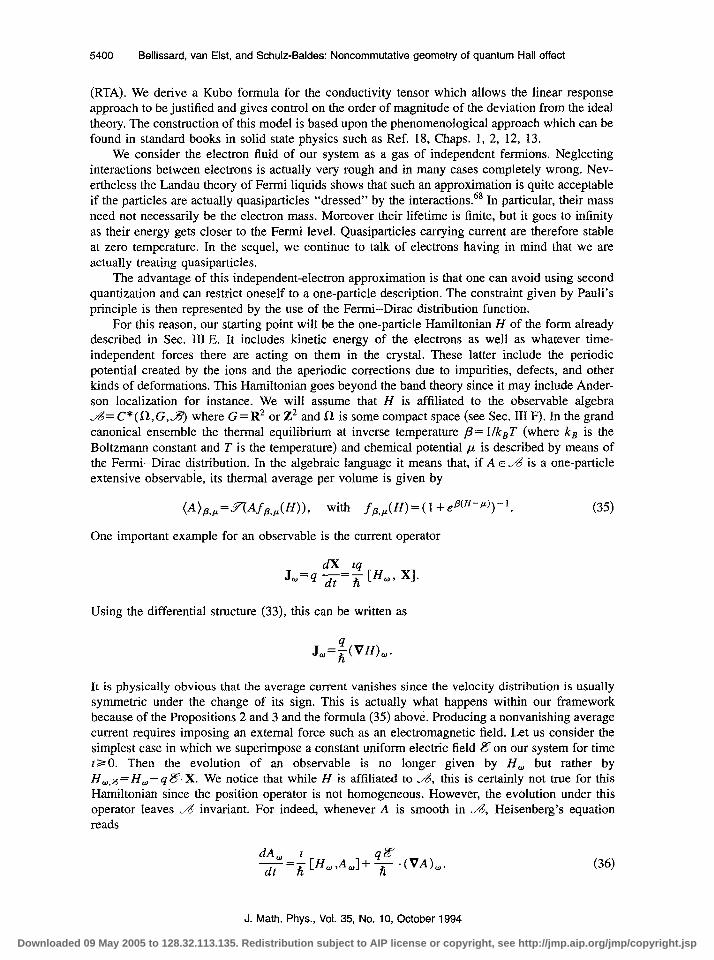
5400 Bellissard, van Elst, and Schulz-Baldes: Noncommutative geometry of quantum Hall effect
(RTA). We derive a Kubo formula for the conductivity tensor which allows the linear response approach to be justified and gives control on the order of magnitude of the deviation from the ideal theory. The construction of this model is based upon the phenomenological approach which can be found in standard books in solid state physics such as Ref. 18, Chaps. 1, 2, 12, 13.
We consider the electron fluid of our system as a gas of independent fermions. Neglecting interactions between electrons is actually very rough and in many cases completely wrong. Nev- ertheless the Landau theory of Fermi liquids shows that such an approximation is quite acceptable if the particles are actually quasiparticles “dressed” by the interactions.68 In particular, their mass need not necessarily be the electron mass. Moreover their lifetime is finite, but it goes to infinity as their energy gets closer to the Fermi level. Quasiparticles carrying current are therefore stable at zero temperature. In the sequel, we continue to talk of electrons having in mind that we are actually treating quasiparticles.
The advantage of this independent-electron approximation is that one can avoid using second quantization and can restrict oneself to a one-particle description. The constraint given by Pauli’s principle is then represented by the use of the Fermi-Dirac distribution function.
For this reason, our starting point will be the one-particle Hamiltonian H of the form already described in Sec. III E. It includes kinetic energy of the electrons as well as whatever time- independent forces there are acting on them in the crystal. These latter include the periodic potential created by the ions and the aperiodic corrections due to impurities, defects, and other kinds of deformations. This Hamiltonian goes beyond the band theory since it may include Ander- son localization for instance. We will assume that H is affiliated to the observable algebra J&= C*(fi,G,J?‘) where G= R2 or Z2 and fl is some compact space (see Sec. III F). In the grand canonical ensemble the thermal equilibrium at inverse temperature p= l/k,T (where kB is the Boltzmann constant and T is the temperature) and chemical potential ,u is described by means of the Fermi-Dirac distribution. In the algebraic language it means that, if A E .A is a one-particle extensive observable, its thermal average per volume is given by
(A)a,+=~Afp,,(H)), with fp+(H)=(l +eP(H-‘LL))-lv
One important example for an observable is the current operator
Jw=q g=; [H,, X].
Using the differential structure (33), this can be written as
J,=+),.
It is physically obvious that the average current vanishes since the velocity distribution is usually symmetric under the change of its sign. This is actually what happens within our framework because of the Propositions 2 and 3 and the formula (35) above. Producing a nonvanishing average current requires imposing an external force such as an electromagnetic field. Let us consider the simplest case in which we superimpose a constant uniform electric field 8 on our system for time t> 0. Then the evolution of an observable is no longer given by H, but rather by H w,K= H,- qg. X. We notice that while H is affiliated to ~5, this is certainly not true for this Hamiltonian since the position operator is not homogeneous. However, the evolution under this operator leaves -4 invariant. For indeed, whenever A is smooth in ~6, Heisenberg’s equation reads
dA, I -=n [H,,A,-j+ F.(VA),. dt (36)
J. Math. Phys., Vol. 35, No. 10, October 1994
Downloaded 09 May 2005 to 128.32.113.135. Redistribution subject to AIP license or copyright, see http://jmp.aip.org/jmp/copyright.jsp
Bellissard, van Elst, and Schulz-Baldes: Noncommutative geometry of quantum Hall effect 5401
If in particular H belongs to A, the right-hand side of (36) stays in .A so that we expect this equation to be integrable within ,A. This can be proved by use of the Trotter product formula.69 We denote by q1 the evolution given by H, namely,
dA)=e I(fi%)Ae-l(f~/fi) (37)
Since H is affiliated to A, this evolution leaves A inyariant and defines a one-parameter group of *-automorphisms of .A Because of formula (34), we also have
This last evolution also leaves -4 invariant. By means of the Trotter product formula we find
erCr”) H~s*n,(A)e-‘(““) Hu.R=.s- lim rTT,(( q!-pql~,,&‘(A)). N-+m
Here, s-lim is the limit in the strong operator topology. So this defines a one-parameter group of automorphisms 7,’ of the von Neumann algebra %Y It represents the evolution of the observables after the electric field has been turned on. We will not investigate here whether this group of automorphisms leaves .A itself invariant. Let us only notice that, whenever H is bounded, a Dyson expansion shows that 7: is an automorphism of .A. Moreover, we only have to work in the Hilbert space L2(.A,fl so that the previous result will be sufficient if H is unbounded. The new current at time t30 is then formally given by
J(t) = v:(J). Since the Hamiltonian Hw,% no longer commutes with H, , the thermal average j(t) = (J( t))a,P of the current will no longer vanish in general. The macroscopic response we expect from a constant uniform electric field is a constant and uniform current, but the microscopic quanta1 forces lead to fluctuations of j(t) in time. To extract the response, it is therefore necessary to consider the time average of this current which is actually what one measures in experiment. For indeed, the typical relaxation time of an apparatus measuring the current is of the order of 1 ms to 1 pus (unless very short times are needed), and this has to be compared with the typical collision time of the order of lOwi3 s for the best conductors. Thus. we set
1 T jp,+K=;+i T
s o dt j(t)=@ S (38)
However, our model does not take collisions into account. Indeed we have
Proposition 4: If the Hamiltonian H is bounded in J$ the projection of the time and thermal averaged current jp,p,)5 along the direction of the electric field 8 vanishes.
Proof. Let us compute 2?. J( t). Using the Heisenberg equation it is easy to see that
dH(t) &J(t)=7 , H(t)= ‘f(H)-
Taking the time average gives us
H(T)-H dt&Y.J(r)= T .
Since H is bounded in norm and since [[a/ = ll~ll, the right hand side vanishes as T-+m. q
J. Math. Phys., Vol. 35, No. 10, October 1994 Downloaded 09 May 2005 to 128.32.113.135. Redistribution subject to AIP license or copyright, see http://jmp.aip.org/jmp/copyright.jsp
5402 Bellissard, van Elst, and Schulz-Baldes: Noncommutative geometry of quantum Hall effect
This result is easy to understand in the one-band approximation. In this case, the electric field produces a time shift of the quasimomentum, namely, k E B I+ k(t) = k- 4 Z?tlTi. Taking the time average is therefore equivalent to averaging over quasimomenta, and this is exactly zero. We point out that this result applies also to models with disorder of the form given in (28). The Anderson model is a special example of such Hamiltonians. More generally, if we accept that transitions to bands far from the Fermi level are essentially forbidden, the effective Hamiltonian is always bounded and the Proposition 4 then leads to the vanishing of the current component parallel to IF.
For these reasons, the presented approach is definitely too ntive. As we already pointed out, collisions occur after time periods very short compared to the time over which we average the current. These collisions produce a loss of memory in the current evolution and are actually responsible for the nonvanishing of the time average. Everything looks like as if time evolution has to be considered over short intervals only. We propose to take collision effects into account by means of the following model: the time evolution is described by the new time-dependent Hamil- tonian Hcoll( t) = H - q g. X+ Wcoll( t) where
Wc,dt)= c Wn&t--l,). ?lEZ
In this expression, the tn’s represent collision times. They are labeled such that . . ..t-.<t0=O<t,<~‘~<t~<t~+*<~~~. Because these times occur randomly, we will assume that the time delays r,= t, - t,- i are independent identically distributed random variables distributed according to Poisson’s law with mean value E( bin) = 7.
The W,,‘s are the collision operators. Their main effect is to produce a loss of memory during the time evolution of the current. This process should enforce thermal equilibrium. In particular, it should not modify the Fermi-Dirac distribution. The only way to respect this constraint is to force the W,,‘s to commute with the Hamiltonian H, but to be random otherwise. More precisely, we will assume that the Wn’s are independent identically distributed random operators, commuting with the Hamiltonian H. Their distribution is supposed to be symmetric under the change of sign W, t+ - W,, . Let then i be the operator acting on .1;5 as
It can be extended to a bounded operator on L2(d’,.Y). Moreover, because of the change-of sign symmetry, it is self-adjoint. Let then ~3~ be the closed subspace of L2(.&,F) generated by bounded functions of H. We will then assume that there is 0s K-C 1 such that
Since W, commutes with H it follows that 2 leaves ~6~ invariant so that it forces any operator A E JA along the direction of H. We will not give explicit examples of such random operators because we will only use the collision eficiency operator k later on, so that it solely characterizes our model. The parameter K is purely phenomenological and represents an efjciency coeficient of the collision process. The smaller K, the more efficient are the collisions. We see that the relax- ation time, namely, the time after which there is a complete loss of memory of the initial evolution, has to be renormalized by the efficiency coefficient. We will see below that rrel= r/( 1 -K) is a good measure for this relaxation time. We will discuss later on how to choose this parameter to fit with real systems.
J. Math. Phys., Vol. 35, No. 10, October 1994
Downloaded 09 May 2005 to 128.32.113.135. Redistribution subject to AIP license or copyright, see http://jmp.aip.org/jmp/copyright.jsp

Bellissard, van Elst, and Schulz-Baldes: Noncommutative geometry of quantum Hall effect 5403
B. Kubo’s formula
We now follow the strategy defined in the previous section and compute the current average with the collisions taken into account. This requires to calculate the evolution operator S&t) between time 0 and t&O, where 5 represents the random variables t=(~,, ,Wn)n,O. It is well known that a kick term like W,&t- tn) produces a contribution erWnlh in the evolution between times t, - 0 and t, + 0, namely, at the kick time.70’71 Therefore, if n 5 1 and fn- i G t< t, , we find
n-1
S&t) = e I(?t,-,)Hra
I-I erWj/tref(rj-fj-I)H~-lB.
j=l
We will now set &(A) = (zlh)[H, A] for A in a suitable dense subalgebra of ~8. This is a *-derivation of -4 because of (37). Therefore, it defines an anti-self-adjoint operator on L2(. &,.Y’). Moreover, the evolution of observables is given by the automorphism
n-l
rrEr=e (t-r,_,)(~~+(q/rz)Kv)
IIe ‘wje(‘j-tj-,)(x,+(9/~)~.V)
,
j=l
where Zw,(A)=(z/h)[ Wj, A]. The operator T$~ may also be seen as a unitary on L2( J&Y). In view of Eq. (38), the time average of this evolution requires the calculation of
where E denotes the average over 5 and S>O. After a straightforward calculation we find
This expression is meaningful because the operator in parentheses has a real part bounded from below by S. The average current is then given by
(39)
We then remark that, for ;;f= 0, the right-hand side of (39) vanishes because licf( H)) =f(H) and &u(H)) = 0 for any function f, whereas ZH is anti-self-adjoint. Subtracting this expression with E=O and using the inner product (AIB)=F(A*B) in L2(.,&,fl, gives
If we assume that the nonlinear tetm in the electric field is negligible, we can let S converge to zero. For indeed, VH and Vfa+(H) are orthogonal to ~6~. Thus it is enough to consider the restriction of the operator S+ ( 1 - &)/T - ZH to the subspace orthogonal to .&., . This restriction has a real part bounded from below by ( 1 - K)/ T> 0. Thus it is an invertible operator. If we do not neglect the nonlinear term, we have to investigate more thoroughly what happens as 610. We will not discuss that matter here and postpone it to a future work. Letting S converge to zero, we will get the Kubo formula for the conductivity tensor:
J. Math. Phys., Vol. 35, No. 10, October 1994 Downloaded 09 May 2005 to 128.32.113.135. Redistribution subject to AIP license or copyright, see http://jmp.aip.org/jmp/copyright.jsp

5404 Bellissard, van Elst, and Schulz-Baldes: Noncommutative geometry of quantum Hall effect
jp+%= a%, with gijz[$)( ~jf~.‘(H)Ibl(l-i:iT--h/H ,iH)- (41)
Let us remark that the quantity in the bracket is dimensionless in 20: the trace 7is a trace per unit volume (so that it has the dimension of the inverse of an area) while the derivative dj has the dimension of a length. In addition h ZH has the dimension of an energy. Therefore, we get CT dimensionless in units of q2/h.
If, in addition, the system is symmetric under rotation by 7r/2 in space, namely, if the Hamil- tonian H and the efficiency operator I; are invariant under such a rotation, then the conductivity tensor can be written in matrix form as
u=( -y(, y,j9 where the Hall conductance is the off-diagonal term crH, while CT// is the direct conductivity.
Let us now consider the limit for which the IQHE is valid. Namely, the electric field is vanishingly small, the temperature is zero, and the relaxation time is infinite. In this limit, the Fermi distribution becomes
lim fp.JW = PF, PTO’
(42)
where PF , the Fermi projection, is the spectral projection onto energy levels lower than the Fermi energy. Here the limit is taken with respect to the norm in ,C,2(.,4,Y). Actually, this result is correct only if the Fermi level EF is a continuity point of the DOS of H. Otherwise the eigen- projection PI~~J corresponding to the eigenvalue EF satisfies Yt( PICKS) > 0 and therefore defines a nonzero element of L2(.&7J. This is what happens for instance in the case of the Landau Hamiltonian whenever E,= (n + 1/2)h w, . Moreover, we need the Fermi projection to be Sobolev dzzerentiable, namely it has to satisfy VP, E L2(~&Y’), otherwise the formal limit is meaning- less. We will see in Sec. V B below that such a condition is related to the finiteness of localization length at the Fermi level. We also need to show that the limit of the derivative of the Fermi distribution is the derivative of its limit. Even though we know this to be true for physically reasonable conditions on H, we will not give the proof here but postpone it to a future work.
On the other hand, in the limit of infinite relaxation time, we are left with the formal expres- sion G’d,H which is meaningless in general. If we formally diagonalize the Hamiltonian H, matrix elements of that expression are given by
(EI JiHIE’) (El(hXH)-ld,~I~‘>= E-E, .
In particular it diverges whenever E-E’ unless the numerator vanishes for some reason. This divergency does, however, not occur in the expression of the conductivity tensor. The reason is that the derivative VP, has nonvanishing matrix elements only between energies E and E’ such that EC EF< E’ or E’ < E,< E. For indeed, if P is a projection and d is a derivation, we see that
dP=d(P*), =s dP=(l-P)dPP+PdP(l-P).
So we need to consider the operators PF%H’diH (1 - PF) and (1 - PF).Zi*diH PF only. We then obtain
Lemma I: If the Fermi level is not a discontinuity point of the DOS of H, and if the Fermi projection is Sobolev dtflerentiable, the following formulas hold
J. Math. Phys., Vol. 35, No. IO, October 1994
Downloaded 09 May 2005 to 128.32.113.135. Redistribution subject to AIP license or copyright, see http://jmp.aip.org/jmp/copyright.jsp
Bellissard, van Elst, and Schulz-Baldes: Noncommutative geometry of quantum Hall effect 5405
P,Fn’JiH (1 -P,)=-~fiP,diP,( I-P,),
ProoJ Let us consider the first formula only, because the other can be treated in the same way (notice however the change of sign). Let B+ be the right-hand side. Then
h%‘n(B+)=P,[H, 6’iPF](l-PF).
Since H commutes with Pr, we find [H, diPF]= - [ diH, PF] (after using basic properties of derivations). This gives immediately
hS’n(B+)=P$tH(l-PF).
Since B + connects only energies below the Fermi level with energies above it, and since the Fermi level is not an eigenvalue of H, ZH is invertible on the subspace of such operators, giving the result of the lemma. Cl
Corollary 2 (IQHE-Kubo Formula): If the Fermi level is not a discontinuity point of the DOS of H, in the zero temperature and infinite relaxation time limit and provided the Fermi projection is Sobolev differentiable, namely, VPF~ L2(.&.T’), the conductivity tensor is given by
2
a,=$ 2zrfiPF[diPF, ajPF]) .
In particular the direct conductivity vanishes.
C. Estimating the deviations from the IQHE limit
Before returning to the IQHE, we want to give some idea of the accuracy of the IQHE-Kubo formulas given in the Corollary 2. We recall that it is obtained under the following conditions:
lil, the area of the sample is considered as infinite; we work within the relaxation time approximation;
(iii) the electric field is vanishingly small; (iv) the temperature is zero; (v) the relaxation time is infinite.
In this section we will evaluate roughly the size of the correction terms whenever one of these conditions is relaxed. We know that the relative error on the IQHE measurement of the universal constant e2/h is of order of 2 X lo-* at best.20 Therefore the neglected terms should be smaller than this number in order that the experiment is reliable.
We will not estimate seriously the finite-size effects even though they are in principle acces- sible to a mathematical estimate within the noncommutative framework. However, it is generally accepted that these effects decrease to zero as e -L’r where L is the sample size and r some typical length. We will choose r to be of the order of magnitude of the localization length. We shall see that it diverges precisely whenever the Hall conductance jumps from one plateau to another. Then as this localization length increases, there is a, critical value beyond which the Coulomb interaction between electrons can no longer be neglected. This is the situation in which the FQHE occurs. To estimate this value, one can define r to be such that the electrostatic energy of a pair of electrons separated by a distance r is of the order of magnitude of the cyclotron energy. This gives r= 1 pm namely, an overestimated large distance compared to the magnetic length. Thus as soon as La20
J. Math. Phys., Vol. 35, No. 10, October 1994 Downloaded 09 May 2005 to 128.32.113.135. Redistribution subject to AIP license or copyright, see http://jmp.aip.org/jmp/copyright.jsp
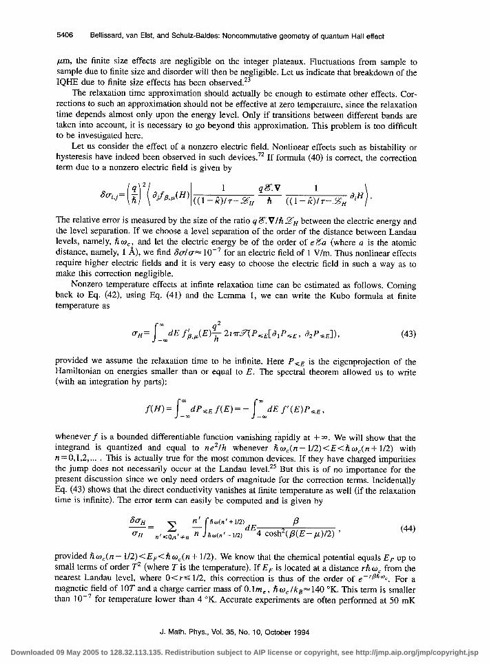
5406 Bellissard, van Elst, and Schulz-Baldes: Noncommutative geometry of quantum Hall effect
pm, the finite size effects are negligible on the integer plateaux. Fluctuations from sample to sample due to finite size and disorder will then be negligible. Let us indicate that breakdown of the IQHE due to finite size effects has been observed.23
The relaxation time approximation should actually be enough to estimate other effects. Cor- rections to such an approximation should not be effective at zero temperature, since the relaxation time depends almost only upon the energy level. Only if transitions between different bands are taken into account, it is necessary to go beyond this approximation. This problem is too difficult to be investigated here.
Let us consider the effect of a nonzero electric field. Nonlinear effects such as bistability or hysteresis have indeed been observed in such devices.72 If formula (40) is correct, the correction term due to a nonzero electric field is given by
The relative error is measured by the size of the ratio 4 8’. Vlii22;, between the electric energy and the level separation. If we choose a level separation of the order of the distance between Landau levels, namely, fi 0, , and let the electric energy be of the order of e&z (where a is the atomic distance, namely, 1 A), we find &/(+a 10m7 for an electric field of 1 V/m. Thus nonlinear effects require higher electric fields and it is very easy to choose the electric field in such a way as to make this correction negligible.
Nonzero temperature effects at infinte relaxation time can be estimated as follows. Coming back to Eq. (42), using Bq. (41) and the Lemma 1, we can write the Kubo formula at finite temperature as
u’H= I cc -02 dE f~,+(E)$2~7r.Y7P,,[d,P,,, ~,P,,l),
provided we assume the relaxation time to be infinite. Here P SE is the eigenprojection of the Hamiltonian on energies smaller than or equal to E. The spectral theorem allowed us to write (with an integration by parts):
f(H)= /yrn dP,,.f(E)= - I
m dE f’(E)PsE, -co
whenever f is a bounded differentiable function vanishing rapidly at + 03. We will show that the integrand is quantized and equal to ne*/h whenever no,(n- 1/2)<E<hw,(n+ l/2) with n=0,1,2 ,... . This is actually true for the most common devices. If they have charged impurities the jump does not necessarily occur at the Landau level.*’ But this is of no importance for the present discussion since we only need orders of magnitude for the correction terms. Incidentally Eq. (43) shows that the direct conductivity vanishes at finite temperature as well (if the relaxation time is infinite). The error term can easily be computed and is given by
SUH
(+H= = 9-;;:f:i;)dE4 cosh*(;E-&,2) ’ n'cO,n'#n (4.4)
provided fi w,( n - l/2) < E,< fi w,( n + l/2). We know that the chemical potential equals EF up to small terms of order T* (where T is the temperature). If EF is located at a distance rho, from the nearest Landau level, where O<rS l/2, this correction is thus of the order of e-‘@“c. For a magnetic field of 10T and a charge carrier mass of O.lm, , fLw,lkB= 140 “K. This term is smaller than 10e7 for temperature lower than 4 “K. Accurate experiments are often performed at 50 mK
J. Math. Phys., Vol. 35, No. 10, October 1994
Downloaded 09 May 2005 to 128.32.113.135. Redistribution subject to AIP license or copyright, see http://jmp.aip.org/jmp/copyright.jsp

Bellissard, van Elst, and Schulz-Baldes: Noncommutative geometry of quantum Hall effect 5407
and magnetic fields can be as high as 18T. Moreover, in heterojunctions, the effective mass of the charge carriers is one order of magnitude smaller. Therefore, the pure temperature effect (at infinite relaxation time) is indeed negligible.
The infinite relaxation time approximation is in fact the most important effect. The relevant parameter is the relaxation time r,,[ = r/( I- K) ; it can be estimated by means of Drude’s formula by measuring conductivities. Assuming the relaxation time to be large, the lowest order contribu- tion to the Hall conductivity is given by [see Eq. (41)]
4* 1 uH=k ~fiP,[~~‘(hP,), a2P,1).
Estimating r/;-,’ by l/w,, we see that the error term due to this contribution is controlled by &=(rWp. For semiconductors used in the IQHE, the mobility /.L~ (c denotes the type of charge carriers) at zero magnetic field and 4.2 OK varies from about lo4 cm*/V s for the MOSFET to lo6 cm*/V s for the AlGaAs or InAs-GaSb heterojunctions (Ref. 20, pp. 40 and 41). These high-mobility devices are used for the FQHE. On the other hand, the effective mass of charge carriers varies from 0.2m, for the MOSFET to O.O3m, for InAs-GaSb heterojunctions. Since rut= ,+9?, we find ~“0.1-0.005 for ..%‘= 1OT. We remark, however, that our relaxation time r,,[ only incorporates time-dependent disorder and may therefore be significantly smaller than the one calculated with Drude’s formula.
It is usually estimated* that the deviation of the Hall conductance from its ideal value is linked to the direct conductivity ali by
Measurements give min( cr,,) c 10 -7 max( a,,) = 10m7e2/h (Ref. 2) so that the relative error on the Hall conductance is indeed of the order of lo-*.
Why is (+,, so small? Looking at the equivalent of Eq. (45) for the direct conductivity, we see that one way to estimate it consists of replacing rH’ by l/o, whereas the remaining terms are related to the localization length X. But since F(PF) =rr is the charge carrier density, we expect this term to be of the order of nX2/r,.,10,. The mobility ,u, of the charge carriers c is r,,[w, /.-%‘. Moreover we introduce the filling factor v= nhlqdt? leading to the very rough estimate
SUH e X2 - sc0nst.v h CL,.
CH
For the heterojunction, v is typically between 1 and 10 at most. The ratio q/h is given by the electron charge e/h and is thus universal. The localization length is always bigger than 80 A. The mobility is at most equal to 2. lo6 cm*/V s for the best heterojunctions. We then find a ratio of the order of 10 -4. Therefore, this estimate is too crude to explain the high accuracy observed in experiment. Nevertheless, it shows that collision effects are dominant whereas localization is a necessity.
In any way, physical arguments indicate 73*20 that because of the small value of the density of states between Landau levels, the leading contribution to the direct conductivity is given by phonon-assisted hopping, at least while the Fermi energy is not too close to a Landau level. Estimation (44) only includes conductivity by thermal activation, whereas (45) only incorporates effects due to a finite collision rate. Here, we shall not treat the interplay of the two phenomena, but only indicate that Mott theory leads to ul/ = o. exp( - (To/T)1’3) in two dimensions, while including Coulomb interaction would give a,,= o. exp( -(To/T) *‘* .74 this latter is in better agree- ), ment with experiment.75
J. Math. Phys., Vol. 35, No. IO, October 1994 Downloaded 09 May 2005 to 128.32.113.135. Redistribution subject to AIP license or copyright, see http://jmp.aip.org/jmp/copyright.jsp

5408 Bellissard, van Elst, and Schulz-Baldes: Noncommutative geometry of quantum Hall effect
D. Dixmier trace and Sobolev space
In this section, we introduce the Dixmier trace and we will prove a formula that can be found in a similar form in a paper by Connes.60 We will see that this tool is a key point both in proving the integrality of the Chem number of a projection and in the study of localization. Most of the material presented here can be found in Refs. 6 and 60 so that we will give no proof unless absolutely necessary.
First, let us recall that, given a separable Hilbert space 33, 3Y(33) is the C*-algebra of compact operators on .%, namely, the norm-closure of the set of finite rank linear operators on 29’. The Schatten ideal 9’(3Y) is defined as the set of compact operators T such that Zr= t ~~<~, where the p,‘s are the eigenvalues of (TT*) 1/2 labeled in the decreasing order. The following proposition summarizes the main properties of Schatten ideals; it can be found in,76V5 for example.
Proposition 5: Let Z’(S) be the algebra of bounded operators on 3V and Tr the usual trace on 53’(3@. Then we have the following:
ii) 2Y(JY)={T~B’(.%j~Tr(~T[P)<~} 57’(S) is a two-sided ideal in Z( &
(iii) (iv)
2Y’(3@ is a Bunach spacefor the norm I/T[I,=(Tr(lTIP))“P=(Z,(p,(T)P))”J’. 24n(3YjCZr(3@ for psq.
(v) Letp,q,s E [l,m) with I/r=I/p+I/q, .SES’(~@ and TE%‘(.%). Then, Holders in- equality holds: Il~~ll,+l$,ll~ll~.
Now we introduce the MaEaev ideals B”(3E) and 23’-(243) and the Dixmier trace.
Definition 4: Let 23 be a separable Hilbert space and .Z be the ideal of compact operators on 3% ForpE[l,m), the Ma;aev ideal %‘+(3?Y)C% is the set of compact operators T of which the characteristic values satisfy
where the characteristic values are the eigenvalues (Pi) of (TT ) * “* labeled in decreasing order. Z%‘-(m is defined in the much same way but with the lim sup equal to zero. We will also set
liTlip+=;y; &5 1~:. ?Z=l
Theorem 7:
(i) 3’ and 2@‘- are two-sided ideals in Z(m. (ii) ForpE[I,w) one has L@‘C%‘-CIP+C~+~Y~>O. (iii) The expression IITll,,+ defines a norm on S’+, making it into a Banach space.
Next, the Dixmier trace is constructed as follows.59 Let Lim be a positive linear functional on the space of bounded sequences I”,(N) of positive real numbers which is translation and scale invariant. If cr E l”+(N) converges, then the functional Lim satisfies:
Lim( cu) = lim LY, . (46) n-+m
J. Math. Phys., Vol. 35, No. 10, October 1994
Downloaded 09 May 2005 to 128.32.113.135. Redistribution subject to AIP license or copyright, see http://jmp.aip.org/jmp/copyright.jsp

Bellissard, van Elst, and Schulz-Baldes: Noncommutative geometry of quantum Hall effect 5409
Scale invariance means that Lim( cu) = Lim( (pi , crl , CY~, CY~, . ..) . To construct Lim, Dixmier uses an invariant mean on the Euclidean group of R (the existence of such means results from a theorem of von Neumann).
Definition 5: For positive T E %” + and a fixed scale-invariant and positive linear functional Lim on l”,(N) satisfying (461, the Dixmier trace is defined by
Remark that T E Z”+ if and only if Troix( 1 TI) < M. Moreover, if the sequence (( 1 /In N) Zf=ipJ converges, then all functionals Lim of the sequence are equal to the limit and the Dixmier trace is given by this limit. From this definition, one can show that Troix is a trace in the following sense:59
Proposition 6: The functional Trni, defined in Definition 5 can be extended as a linear form on Z’+ such that:
(i) positivity: if TE LZ”+ is a positive operator then Trn;,(T)>O, (ii) trace property: if S, T E 3’ ’ then Troix( ST) = Trn,( TS) , (iii) unitary invariance: if T E Z’+ and U is unitary then Trnix( UTU-‘) =Tr& T), (iv) ;t$ity: it is continuous with respect to the seminorm IITII1+ . Moreoven Trni, vanishes
Let us introduce the operator $ acting on a linear operator A on 12(G) as
g~=[u,~], x1 + 1x2
u= IXlflXZI ’
where Xi ,X2 are the components of the position operator. The main result of this section is given by the following proposition.
Proposition 7: Let R be a compact metrizable space on which G acts by homeomorphisms. Let P be a G-invariant ergodic probability on 0. One then denotes by ,& the @=-algebra of this dynamical system and by rthe trace on ~3 corresponding to P. Let J$ be the dense subalgebra of continuous functions with compact support on OXG.
Then for every A E J&, the following formula holds:
s(lVAl’)=~ Tr,,(I$A,j2), for P-almost all w. (47)
If Lf denotes the Sobolev space associated to .c this formula can be continued to elements A ~7. In particular $AEY, then &,ES~’ for P-almost all o.
In the remaining part of this section we present the proof of Proposition 7 for the case of discrete physical space G = Z2; the continuous case will be treated in future work.64 The first step in this proof is the following lemma:
Lemma 2: Let T be a bounded operator on &ZD) such that
(i) 3r such that (n/Tlm)=O V/n-ml2r. (ii) There exists a positive constant C such that I(nlqm)lsC/(I +InlDjVm EZ~.
T is then in the MaEhev ideal St’ and, for any linear functional Lim, its Dixmier trace can be calculated by
J. Math. Phys., Vol. 35, No. 10, October 1994
Downloaded 09 May 2005 to 128.32.113.135. Redistribution subject to AIP license or copyright, see http://jmp.aip.org/jmp/copyright.jsp
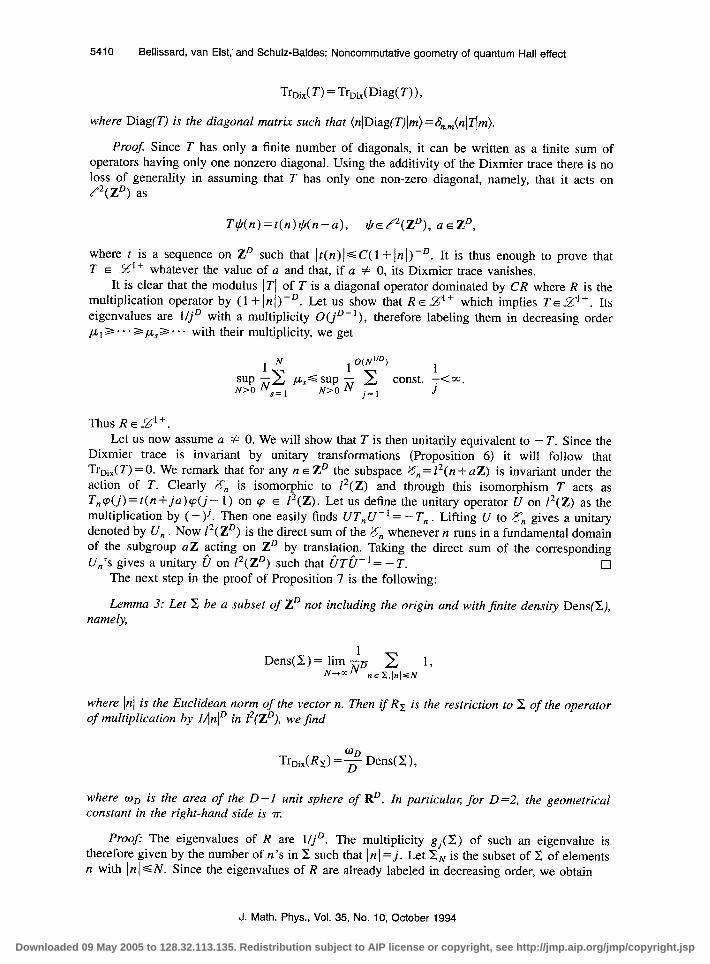
5410 Bellissard, van El&,’ and Schulz-Baldes: Noncommutative geometry of quantum Hall effect
TroiX( T) = TrADiag( T)),
where Diag(T) is the diagonal matrix such that (n~Diag(T)~m)=S,,,(n~Tjm).
Proof. Since T has only a finite number of diagonals, it can be written as a finite sum of operators having only one nonzero diagonal. Using the additivity of the Dixmier trace there is no loss of generality in assuming that T has only one non-zero diagonal, namely, that it acts on P(ZD) as
T+(n)=t(n)+(n-a), @IE&Z~), aEZD,
where t is a sequence on ZD such that I t(n)/ G C( 1 + Inl)-D. It is thus enough to prove that T E K’+ whatever the value of a and that, if a # 0, its Dixmier trace vanishes.
It is clear that the modulus ITI of T is a diagonal operator dominated by CR where R is the multiplication operator by ( 1 + InI) -D. Let us show that R E 23’* + which implies T E 55”+. Its eigenvalues are l/jD with a multiplicity O(jD-’ ), therefore labeling them in decreasing order p,>...>p+-... with their multiplicity, we get
IN 1 O(N”D) sup -C pu,=G sup -
N>O Ns=l C
1
N>ON const. T<W.
]=I J
Thus REP’+. Let us now assume a # 0. We will show that T is then unitarily equivalent to - T. Since the
Dixmier trace is invariant by unitary transformations (Proposition 6) it will follow that Troi,( T) = 0. We remark that for any n E ZD the subspace & = 12(n + aZ) is invariant under the action of T. Clearly 2Yn is isomorphic to 12(Z) and through this isomorphism T acts as T,cp(j)=t(n+ja)q(j- 1) on cp E 12(Z). Let us define the unitary operator U on l*(Z) as the multiplication by (-)‘. Then one easily finds UT,,U-‘= -T,, . Lifting U to 2Yn gives a unitary denoted by U, . Now 12( ZD) is the direct sum of the En whenever n runs in a fundamental domain of the subgroup aZ acting on ZD by translation. Taking the direct sum of the corresponding Un’s gives a unitary fi on 12(ZD) such that CT&’ = - T. 0
The next step in the proof of Proposition 7 is the following:
Lemma 3: Let c be a subset of ZD not including the origin and with finite density Dens(C), namely,
Dens(C)= lim & 2 1, N--r- tZ.P,l?llSN
where InI is the Euclidean norm of the vector n. Then if Rx is the restriction to 2 of the operator of multiplication by I&ID in 12(ZD), we jnd
TrDix(Rr)=$ Dens(X),
where wg is the area of the D-I unit sphere of RD. In particular, for D=2, the geometrical constant in the right-hand side is rr.
Proof: The eigenvalues of R are l/j D. The multiplicity gj(C) of such an eigenvalue is therefore given by the number of n’s in 2 such that InI =j. Let ZN is the subset of 2 of elements n with 1 n 1 G N. Since the eigenvalues of R are already labeled in decreasing order, we obtain
J. Math. Phys., Vol. 35, No. 10, October 1994
Downloaded 09 May 2005 to 128.32.113.135. Redistribution subject to AIP license or copyright, see http://jmp.aip.org/jmp/copyright.jsp

Bellissard, van Elst, and Schulz-Baldes: Noncommutative geometry of quantum Hall effect 5411
(48)
where I Z,vl denotes the number of points in ZCN. Using the definition of the density of a subset, we see that, as j -+ ~0, the multiplicity gj(2) is asymptotically given by the product of the density of 8 by the volume between the balls of radii j - 1 and j. Namely,
gj(x) em Dens(C) oo jD-‘.
In much the same way, we get lZNl Nz” Dens(C) an ND if fi2, is the volume of the unit ball of RD. Taking the logarithm we are left with Dln N+O(l) in the expression of the Dixmier trace of Rz . Plugging all these relations in Eq. (48), we get the result. 0
The last technical step in the proof of Proposition 7 is provided by the following lemma where the dimension is D=2.
Lemma 4: Let f be a continuous non-negative function on 0 and a E Z2, a # 0. Let Fz the operator on p(ZZ2) defined by
Then FE E 55” ’ and its Dixmier trace is given by
‘bdF~)=~ kd2/ dP(olf(w), for P-almost every w E R.
Proofi AS In I --+w the function
*(nl=li - f+i2, admits the asymptotics (p(n) bl,m Ial2 sin2 cx&z/2 modulo terms of order l/In I 3, where cy,, is the angle between the directions of a and n.
Let US now slice the space R according to the finite partition {nj, a}, where 6> 0 is small enough and j an integer such that ~j,, is the set of points o for which (j - l/2) Ss f (0) C (j + 112) S. Since f is continuous with compact support, it is bounded so that only a finite number of j’s are needed here. Let then Cj,a(W) be then set of n’s in Z2 such that T-“wE~j 6. Using Birkhoff’s ergodic theorem, for P-almost every o, Zj,~ 0) has a finite density givkn by the probability P( fl j, J.
We then slice Cj,* into a finite subpartition {Xj,s,r} where Xj,a,r corresponds to those points n E Cj,s for which (r- l/2) 6s a,<(r+ l/2)8. Thus modulo an error of order O(s) we get f(T-nw)cj(n)=la12 jS sin2(r6)(1+0(S))lln12 on 2j.s.r. Moreover since this slicing concerns only a finite partition it permits to write Fz as a finite sum, namely,
F:=c i,r F:k, 6r. . .
J. Math. Phys., Vol. 35, No. 10, October 1994 Downloaded 09 May 2005 to 128.32.113.135. Redistribution subject to AIP license or copyright, see http://jmp.aip.org/jmp/copyright.jsp
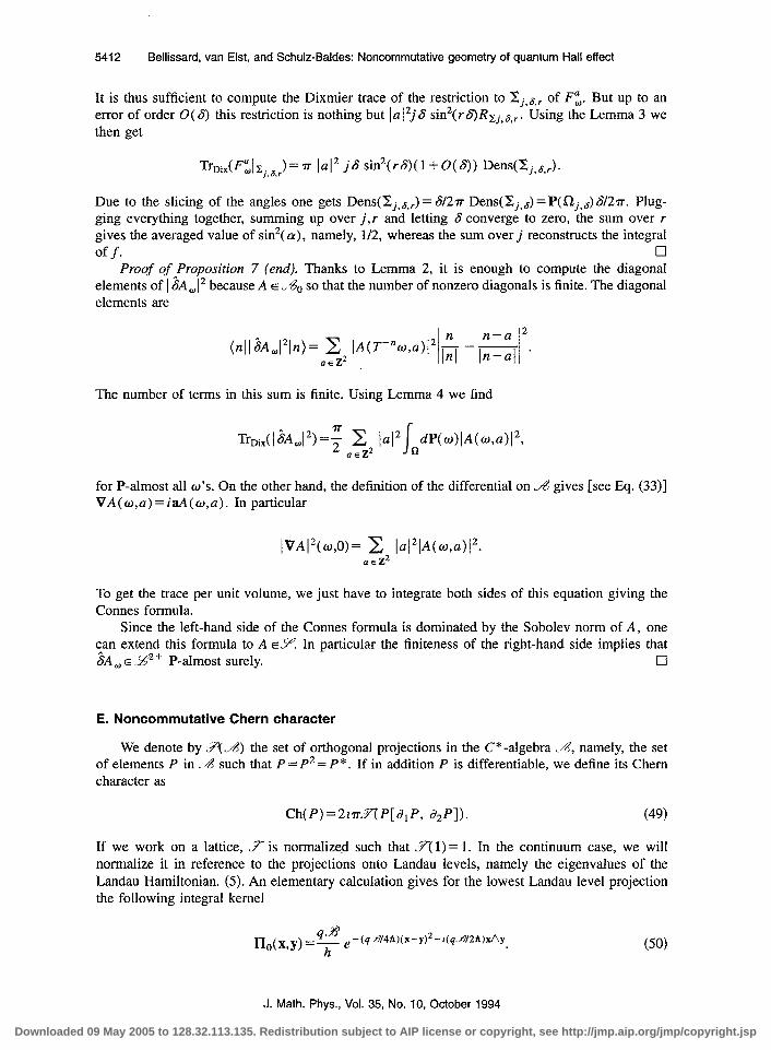
5412 Bellissard, van Elst, and Schulz-Baldes: Noncommutative geometry of quantum Hall effect
It is thus sufficient to compute the Dixmier trace of the restriction to Cj,S,r of Fz. But up to an error of order 0( 6) this restriction is nothing but Ia 12jS sin2( rG)Rxj,8,r. Using the Lemma 3 we then get
TrniX(FzIZj 6r)=m 1~1~ jS sin2(r8)( 1 +O( 8)) Dens(Xj,s,,.). . 1
Due to the slicing of the angles one gets Dens(Cj,J,,) = S/27r Dens(Cj,~)=P(Rj,~) 6/27r. Plug- ging everything together, summing up over j,r and letting 6 converge to zero, the sum over r gives the averaged value of sin2( a), namely, l/2, whereas the sum over j reconstructs the integral off. 0
Proof ofProposition 7 (end). Thanks to Lemma 2, it is enough to compute the diagonal elements of 1 SA,12 because A E ~&?a so that the number of nonzero diagonals is finite. The diagonal elements are
(nll$Aw121n)= c IA(Z--” aaZ2
The number of terms in this sum is finite. Using Lemma 4 we find
for P-almost all 0’s. On the other hand, the definition of the differential on . R gives [see Eq. (33)] VA(o,u)=iaA(o,u). In particular
To get the trace per unit volume, we just have to integrate both sides of this equation giving the Connes formula.
Since the left-hand side of the Connes formula is dominated by the Sobolev norm of A, one can extend this formula to A EY. In particular the finiteness of the right-hand side implies that $A w E -Y??+ P-almost surely. 0
E. Noncommutative Chern character
We denote by 3~6) the set of orthogonal projections in the C*-algebra -4, namely, the set of elements P in ..J such that P= P2= P*. If in addition P is differentiable, we define its Chern character as
Ch(P)=2mflP[d,P, c?,P]). (49)
If we work on a lattice, 3 is normalized such that .T( 1) = 1. In the continuum case, we will normalize it in reference to the projections onto Landau levels, namely the eigenvalues of the Landau Hamiltonian. (5). An elementary calcuiation gives for the lowest Landau level projection the following integral kernel
sx -(q A/4h)(x-y)‘-r(q.A/2t)~y. J&(x,Y) =h e (50)
J. Math. Phys., Vol. 35, No. 10, October 1994
Downloaded 09 May 2005 to 128.32.113.135. Redistribution subject to AIP license or copyright, see http://jmp.aip.org/jmp/copyright.jsp

Bellissard, van Elst, and Schulz-Baldes: Noncommutative geometry of quantum Hall effect 5413
In particular, ITa defines an element of ,&= C*(a,R2,Z) for any choice of the hull 0. In much the same way, we denote by III, the projection on the nrh Landau level (n=0,1,2 ,... ). We then deduce the following results.
Lemma 5: The trace and the Chem character of the Landau levels are given by
;7(I-I.)=y) Ch(II,)= - 1. (51)
ProoJ Let us prove this result for II, first. Its trace per unit volume is given by the space average of IIu(x,x) = q-S/h. This gives the first formula in (51). To compute its Chem character, we remark that Vl$(x,y) = - z(x-y)IIa(x,y). Introducing the complex variables .X=X, + zx2 and Y=Y~+zY~, weget
To compute this integral, we develop the exponential in powers of x7 and notice that all contri- butions vanish except the one involving the term l~]~ly]~. Th e corresponding integral has sepa- rated variables and can be computed explicitly. This gives - 1.
For the other Landau levels, we remark that III,-- II, in the sense of von Neumann equiva- lence (see below). More concretely, it is enough to exhibit an element U, E & such that II,= U,*U, and ITa= U,U,* . This implies that the traces are identical and we will show their Chem characters to be identical as well (see Lemma 11 below). To construct U, , we introduce the annihilation operator
Then [a, a*] = 1. Thus au * is bounded below by 1 and is invertible. We set u = (au*) - ‘Da and U,=rI()zP. It is easy to check that UU* = 1 implying that II, = U,,U,* . On the other hand, U,* U, = a *“lI,u”ln ! . But it is a standard result that we obtain the nth Landau level by applying the creation operator n times to the ground state, namely, In > = ( l/fi)u *n]O). In particular a *“IIl,a”ln ! = lI, .
It remains to show that U, E .&. A straightforward calculation gives U, = (n !) - 1’2110un. Now using the explicit form of the matrix elements (50) and of a, we get the matrix elements of U, in the form of a polynomial in x and y times IIe(x,y), showing that U,(O,x) is absolutely summable in x. This is enough to show that it belongs to ~3 (see Sec. III F). 0
Our next step will be the von Neumann equivalence. Namely, if P,Q ES(&), then P-Q if there is UEJ% such that P=U*U,Q=UU *. In particular if P is trace class, it follows that Y(P) =3(Q) then. The following results can be found in Ref. 77.
Lemma 6: Let PQ&-&@ be such that IlP-Qll<Z. Then P-Q.
Lemma 7: If & is separable, then the set of equivalence classes of projections in ~8 is at most countable.
Lemma 8: Let P,QEF(&) be two mutually orthogonal projections (namely, PQ=QP=O). Then the equivalence class of their sum P@Q depends only upon the equivalence classes of P and Q. This defines a commututive and associative composition law on the set of equivalence classes, which we denote by [P@Q]=[P]+[Q].
See Refs. 79 and 61, Lemma 4.2.3 for a proof.
J. Math. Phys., Vol. 35, No. IO, October 1994 Downloaded 09 May 2005 to 128.32.113.135. Redistribution subject to AIP license or copyright, see http://jmp.aip.org/jmp/copyright.jsp

5414 Bellissard, van Elst, and Schulz-Baldes: Noncommutative geometry of quantum Hall effect
Remark that we can add only mutually orthogonal projections in this way, because the sum of two projections is not a projection in general. So giving any pair P,Q of projections it is not always possible to find equivalent projections P ’ - P and Q ’ - Q such that P’ and Q ’ be orthogo- nal. In other words the sum is not everywhere defined in Fiji). In order to deal with this problem, we replace the algebra ,/A by its stabilization, namely, the tensor product &8.% with the algebra of compact operators on a separable Hilbert space, which is nothing but the smallest C*-algebra containing all finite dimensional matrices. Then it is possible to show that one can always choose pairs of projection as orthogonal up to equivalence. By the Grothendieck method one builds a group out of the equivalence classes of projections of ,&3X. This group is denoted Ko(&3) (see Refs. 78 and 61, Theorem 10.
Lemma 9: For any P~fi&) there is a differentiable projection PO ~3-4) such that P-Ppo.
This last result is a consequence of the fact that the set of differential elements in .A is norm dense.
Lemma IO: For any pair PQ ~fl.fn) of equivalent projections and any E small enough, there are differentiable projections P, ,Q, ~3~6) and a differentiable element U, such that IIpe-pII~~j IleE-QII s E and P, = U,U,* whereas Q, = Ut U, .
The proof is straightforward: it follows from the density of E?” (.A) and from the proof of Lemma 6. We will say that P and Q are smoothly equivalent whenever the element U which connects them can be chosen differentiable.
Lemma 11: For any pair P Q E-J&) of smoothly equivalent projections Ch(P) =Ch(Q).
The proof of this result is purely combinatorial provided we use the cyclicity of the trace E We will omit it here.4
Lemma 12: For any pair PQE~~&) of mutually orthogonal smooth projections we have Ch(P@Q, =Ch(P) fCh(Q).
The proof of this result is standard and can be found in Ref. 4 for instance. To summarize this set of results we have
Theorem 8: The Chem character Ch defines a group homomorphism from Ko(. A) into a countable subgroup of the real line.
It remains to show that the image of this map is the set of integers. This will be done in Sets. IV F and IV G.
F. Connes formulas
In order to compute eventually the Chem character of a projection, we need an intermediate tool, namely, a cyclic cocycle. This is actually the heart of Connes work on the noncommutative extension of cohomology. Here, we shall actually only need a 2-cocycle r2, which is a trilinear form on the algebra A0 defined by
Y2(A0,A1,A2)=2rrzflA0d,AlJ2A2-AOd2AIdlA2). (52)
By the Schwarz inequality for the trace 7, we see that r2 can be extended to the noncommu- tative Sobolev space .Y, which is linear subspace of the von Neumann algebra 3Y. The proof of the following lemma is algebraic and standard by now; it can be found in Ref. 4.
Lemma 13: 72 is a 2-cocycle, i.e., it satisfies the following algebraic properties:
J. Math. Phys., Vol. 35, No. 10, October 1994
Downloaded 09 May 2005 to 128.32.113.135. Redistribution subject to AIP license or copyright, see http://jmp.aip.org/jmp/copyright.jsp

Bellissarci, van Elst, and Schulz-Baldes: Noncommutative geometry of quantum Hail effect 5415
(i) Y2 is cyclic: Y&A0 ,A 1 ,A2) =Y2(A2 ,A0 ,A I), (ii) Y2 is closed under Hochschild’s boundary operatool; that is: b:
-Y2(A3Ao,AI ,A,)=O.
We will now give a formula which permits to compute the cocycle r2 by means of the physical representations. For this purpose, we present the formalism introduced by Connes4 (we already gave some indications in Sec. III B ). A graded Fredholm mo$le is defined as follows. Let X+ and .X- be two separable Hilbert spaces; their di:ect sum %‘=%+ @ 2K becomes a graded Hilbert space through the graduation operator G equal to + 1 on A%:, . A representation ~:9--+~(&) of an algebra 9is said to be trivially graded, if [&(A), G] =0 for all A E %. One says that $A) is of degree 0; operators on .% which anticommute with the graduation operator 6 are said to be of degree 1. Any operator on &can be uniquely decomposed into the sum of an operator of degree 0 with an operator of degree 1.
De$nition 6: A Fredholm module is a family (B,&,?r,F) where B is an algebra with a trivially graded representation & on a graded, separable Hilbert space 2% and where FE J%‘(& is a self-adjoint operator such that the following three conditions are satisjed:
(i) F6=-6F, (ii) F2=1, (iii) [~~(A),F]E%VAE%?
Here X is the ideal of compact operatorsAon 2%. An elemen! A E 9 is called p-summable (resp. p+-summable) whenever [ii(A), F]E#(%~) (resp. ~9+(%‘)).
The graded commutator of two graded operators T, T’ E 23’(& is defined by
[‘f’, T’ls= TT’ _ ( _ l)d”(T)d”(T’)T’ T.
This commutator extends to the whole algebra Z’(& by bilinearity. The noncommutative differ- ential is given by
dT=[F, T],, TEE@&.
One can check that it obeys the graded Leibniz rule d(TT’) =dT T’+( -)dO(T)T dT’ and that d2 = 0. Finally, the graded trace or the supertrace is defined by
Trs( T) = iTr( &FdT),
whenever the right-hand side is well defined. Here, Tr is the usual trace in Z’( 5%‘). Remark that Trs is linear and satisfies:
Trs( TT’ ) = ( - 1 )dO(T’)dO(T)Trs( T’ T).
Moreover, if dO( T) = 1, then Trs( T) = 0. Now we shall consider the concrete family of Fr:dholm modules which will be of interest to
us. The algebra will be ~6~. The Hilbert space is X=5@ @ X =L2(G) @ L2( G) (where G = R2 or G = Z2) and for A E A0 the representation is given by
, A,= v,(A),
where rro is the family of representations defined in (31). Next
J. Math. Phys., Vol. 35, No. 10, October 1994
Downloaded 09 May 2005 to 128.32.113.135. Redistribution subject to AIP license or copyright, see http://jmp.aip.org/jmp/copyright.jsp
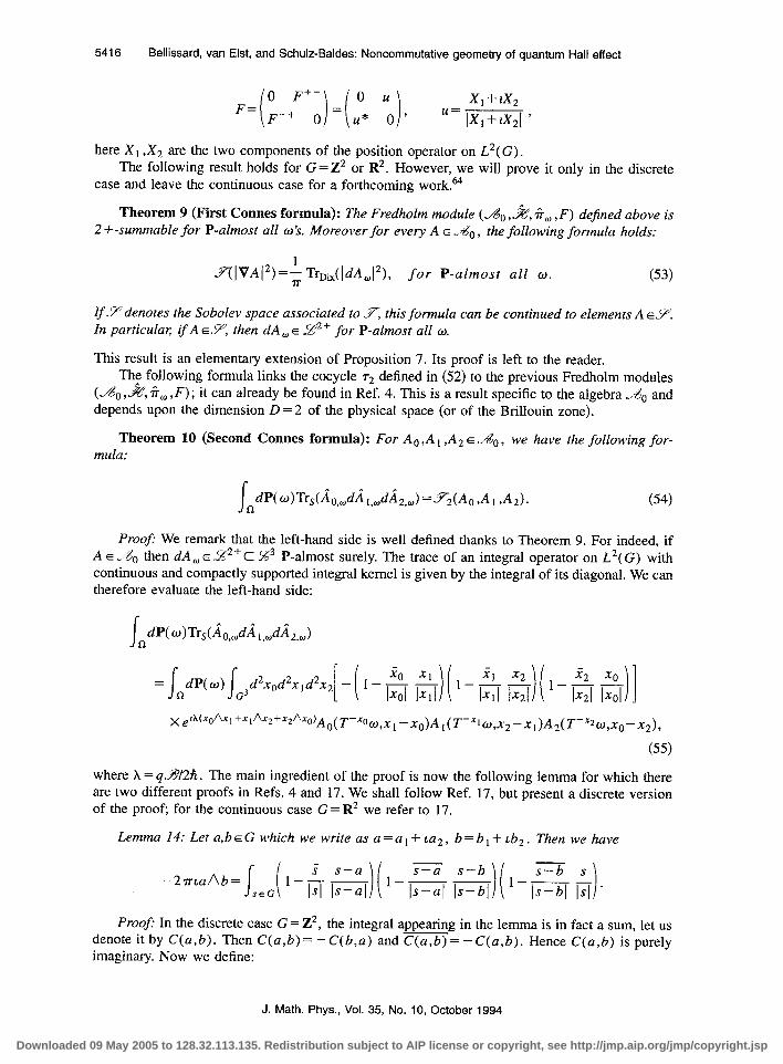
5416 Bellissard, van Elst, and Schulz-Baldes: Noncommutative geometry of quantum Hall effect
F=( ;e+F+,) =(;* “0) u= ,$T;;;, ,
here XI ,X2 are the two components of the position operator on L2(G). The following result holds for G=Z2 or R2. However, we will prove it only in the discrete
case and leave the continuous case for a forthcoming work.@
Theorem 9 (First Connes formula): The Fredholm module (~60 ,&, 6,) F) defined above is 2 +-summable for P-almost all wk. Moreover for every A E ~60, the following formula holds:
Y(IVAi’)=$ TrDix(IdA,/2), for P-almost all w. (53)
If Ydenotes the Sobolev space associated to Y, this formula can be continued to elements A EY: In particular tfA EY, then dA, E 2’ for P-almost all w.
This result is an elementary extension of Proposition 7. Its proof is left to the reader. The following formula links the cocycle r2 defined in (52) to the previous Fredholm modules
(ASo ,.A?‘, ii,,, , F); it can already be found in Ref. 4. This is a result specific to the algebra -<do and depends upon the dimension D = 2 of the physical space (or of the Brillouin zone).
Theorem 10 (Second Connes formula): For A,,A I ,A2 E A,, we have the following for- mula:
I n dP(o)Trs(~o,od~~,,d~2,,)=~(A0,A1,A2). (54)
Proof We remark that the left-hand side is well defined thanks to Theorem 9. For indeed, if A E A0 then dA, E 9’ CLS3 P-almost surely. The trace of an integral operator on L2( G) with continuous and compactly supported integral kernel is given by the integral of its diagonal. We can therefore evaluate the left-hand side:
I n dP(~)Trd&,J~ ,,J~,,,)
= /odP(w) /03d2X,d2x,d2x2 [-(l-~~)(l-~~)(l-~~)]
where X = q3’/2h. The main ingredient of the proof is now the following lemma for which there are two different proofs in Refs. 4 and 17. We shall follow Ref. 17, but present a discrete version of the proof; for the continuous case G = R2 we refer to 17.
Lemma 14: Let a,b E G which we write as a = a 1 + La2, b = b I+ Lb2. Then we have
-2rrLaAb=
Proof In the discrete case G = Z2, the integral appearing in the lemma is in fact a sum, let us denote it by C(a,b). Then C(a,b) = - C(b,a) and C(a,b) = - C(a,b). Hence C(a,b) is purely imaginary. Now we define:
J. Math. Phys., Vol. 35, No. 10, October 1994
Downloaded 09 May 2005 to 128.32.113.135. Redistribution subject to AIP license or copyright, see http://jmp.aip.org/jmp/copyright.jsp
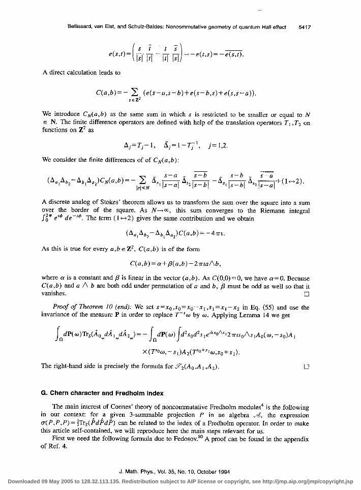
Bellissard, van Elst, and Schulz-Baldes: Noncommutative geometry of quantum Hall effect 5417
e(s,t)= ?- - - 4 -!- = -e(t,s)= -e(s,t). i Isl l:I I4 I4 -1
A direct calculation leads to
C(d)=- 2 ( e s ( - a,s-b)+e(s-b,s)+e(s,s-a)). SEZ2
We introduce C,( a,b) as the same sum in which s is restricted to be smaller or equal to N E N. The finite difference operators are defined with help of the translation operators T, ,T2 on functions on Z2 as
Aj=Tj- 1, bj= l-T~~‘, j= 1,2.
We consider the finite differences of of CN(a,b):
A discrete analog of Stokes’ theorem allows us to transform the sum over the square into a sum over the border of the square. As N--too, this sum converges to the Riemann integral J-o f 2a e’$ de-‘” The term (1~2) gives the same contribution and we obtain
As this is true for every a,b E Z2, C(a,b) is of the form
C(a,b)=a+P(a,b)-2maAb,
where LY is a constant and /3 is linear in the vector (a, b) . As C( 0,O) = 0, we have cy = 0. Because C(a,b) and a A b are both odd under permutation of a and b, /3 must be odd as well so that it vanishes. cl
Proof of Theorem 10 (end): We set s=~~,s~=x~-x~,s~=~~-x~ in Eq. (55) and use the invariance of the measure P in order to replace TeSo by w. Applying Lemma 14 we get
I odP( W)Trs(AoydiIwdA2,) = - ~~dP(o)~d2sod2s~e’“S~AS~2msoh~Ao(w,-so)A,
X(TSow,-s,)A2(TSo+sl wso+sl).
The right-hand side is precisely the formula for Y2(Ao,A 1 ,A,). 0
G. Chern character and Fredholm index
The main interest of Connes’ theory of noncommutative Fredholm modules4 is the following in our context: for a given 3-summable projection P in an algebra JA, the expression a( P, P, P) = iTr,( fidgdp) can be related to the index of a Fredholm operator. In order to make this article self-contained, we will reproduce here the main steps relevant for us.
First we need the following formula due to Fedosov.*’ A proof can be found in the appendix of Ref. 4.
J. Math. Phys., Vol. 35, No. 10, October 1994 Downloaded 09 May 2005 to 128.32.113.135. Redistribution subject to AIP license or copyright, see http://jmp.aip.org/jmp/copyright.jsp
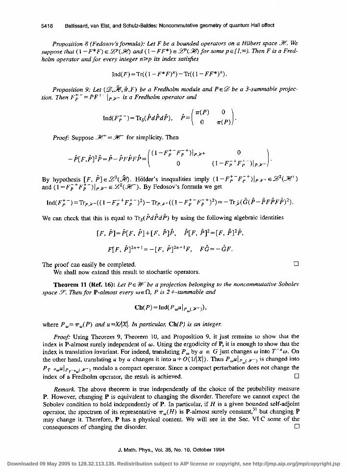
5418 Bellissard, van Elst, and Schulz-Baldes: Noncommutative geometry of quantum Hall effect
Proposition 8 (Fedosov’s formula): Let F be a bounded operators on a Hilbert space B. We suppose that (1 - F*F) E fl(%‘) and (I- FF*) E L%‘(.%) for some p~[l,m). Then F is a Fred- holm operator and for every integer nap its index satisfies
Ind(F)=Tr((l-F*F)“)-Tr((l-FF*)“).
Proposition 9: Let (L@,&,&,F) be a Fredholm module and PEG be a 3-summable projec- tion. Then Fp’ - = P F f - 1 r,x- is a Fredholm operator and
Proof Suppose .%+ = K for simplicity. Then
-P[F,P]~E;=P-PFPFP= (1 -F;-F;+h+ 0
0 (1 -F;+F;-)]P.x-
By hypothesis [F, i] E Z’3(&. Holder’s inequalities imply (1 - F;-Fp+)lp,K+ E L@(w) and (1 - F,fF,f-)lp,r E L??( 5K). By Fedosov’s formula we get
Ind(Fi-)=Trp.K-((l-FP F, -’ +-)2)-Tr~.X+((1-Fpf-Fp+)2)=-Tr,>(&~-~F~F~)2).
We can check that this is equal to Trs(kdfid@) by using the following algebraic identities
[F, P]=I;[F, P]+[F, PII;, P[F, P12=[F, P12P,
F[F, P]2n+‘= -[F, P12”+‘F, F6= -6F.
The proof can easily be completed. We shall now extend this result to stochastic operators.
!J
Theorem 11 (Ref. 16): Let PE 5%‘” be a projection belonging to the noncommutative Sobolev space Y. Then for P-almost every WE 0, P is 2 +-summable and
where P,= r,(P) and u =4X1. In particular, Ch(P) is an integer.
Proof: Using Theorem 9, Theorem 10, and Proposition 9, it just remains to show that the index is P-almost surely independent of w. Using the ergodicity of P, it is enough to show that the index is translation invariant. For indeed, translating P, by a E G just changes o into Team. On the other hand, translating u by a changes it into u + 0( lllX[). Thus P,ulr,(x-) is changed into PT-Oo~lpr-,oC,X-) modulo a compact operator. Since a compact perturbation does not change the index of a Fredholm operator, the result is achieved. 0
Remark. The above theorem is true independently of the choice of the probability measure P. However, changing P is equivalent to changing the disorder. Therefore we cannot expect the Sobolev condition to hold independently of P. In particular, if H is a given bounded self-adjoint operator, the spectrum of its representative r,(H) is P-almost surely constant,31 but changing P may change it. Therefore, P has a physical content. We will see in the Sec. VI C some of the consequences of changing the disorder. cl
J. Math. Phys., Vol. 35, No. 10, October 1994
Downloaded 09 May 2005 to 128.32.113.135. Redistribution subject to AIP license or copyright, see http://jmp.aip.org/jmp/copyright.jsp

Bellissard, van Elst, and Schulz-Baldes: Noncommutative geometry of quantum Hall effect 5419
H. Quantization, Fredholm, and relative index
In this section, we will discuss the links between the Laughlin argument as presented in Sec. II E and our approach. The essential ingredient for that will be the relative index of two projec- tions as defined by Avron, Seiler, and Simon.17 It turns out that the singular gauge transformation of Laughlin corresponds to the unitary operator u=X/IXI. Thus the charge transported after changing the flux by one quantum is then exactly given by the index we computed in Theorem 11. The main improvement upon Laughlin’s argument is that we control completely the effect of the disorder now, since this index is a topological invariant. Let us remark that the topology we are talking about is the one of the Brillouin zone and not of the sample as can be erroneously derived from a superficial understanding of Laughlin’s argument.
More precisely, following Sec. II E, let the varying flux be 4(t) = fitler with r so large as to produce an adiabatic change. Then at time t= 7 the new Hamiltonian in (8) is given by
H,A$=uH,AO)u*, u= 6,
namely, the phase of the wave function changes by ere where t9 is the polar angle of the position x. Formally, one gets an equivalent formula at each intermediate times, but the domains change with time. The Eq. (56) implies for the corresponding Fermi projections:
PF(,r)=UPF(O)U*, W)=xeFW.AtN. (57)
The charge transported to infinity after this adiabatic change is the number of states in PF( 7) that are not in PF(0). Since both projections are infinite dimensional, we must be careful in computing this number. It is the purpose of the following definition17 to take care of this difficulty. Namely, given two projections P and Q on a Hilbert space we set
Index(P,Q)=dim(Ker(P-Q- l))-dim(Ker(Q-P- l)),
whenever the right side is well defined. Then (see Ref. 17 for a proof)
Proposition 10: Let P and Q be two projections on Hilbert space. If (P-Q) E %‘, then for every integer m such that 2m+l >p, the relative index can be calculated as
We then apply this formalism to the 2 + -summable Fermi projections P,,, and u PF,,,u*. It is an immediate consequence of the proof of Proposition 9 that
(58)
which is P-almost surely equal to - Ch( PF). The suitable p = 2m + 1 is p = 3 here. We remark that it is the smallest possible one giving a nonzero relative index because, if P,- UP+* were trace class, the relative index would vanish. Hence the Chem character of the Fermi projection can be identified up to sign, with the charged transported at infinity during the adiabatic flux change. Let us then call this index the charge dejiciency index.
Owing to the stability of the Fredholm index, if one pierces the flux tube at some other place than the origin and then uses another unitary operator than u = e”, the Fredholm index will not change. Moreover, adding some disorder potential to the Landau Hamiltonian will not change the index as well as long as the Fermi projection belongs to the Sobolev space (we will discuss this condition more precisely in the next section).
J. Math. Phys., Vol. 35, No. 10, October 1994
Downloaded 09 May 2005 to 128.32.113.135. Redistribution subject to AIP license or copyright, see http://jmp.aip.org/jmp/copyright.jsp

5420 Bellissard, van Elst, and Schulz-Baldes: Noncommutative geometry of quantum Hall effect
V. LOCALIZATION AND NONCOMMUTATIVE SOBOLEV SPACE
In this chapter, we relate the Sobolev condition on Fermi projections to the Anderson local- ization. We will give several mathematical tools to describe rigorously localization in terms of our formalism. The main results are Theorems 13 and 14 below. As a consequence, the remaining results in the main Theorem 1 follow.
In Sec. V A we review the well-known Anderson-Pastur criterion for localization. Then we give a new definition of the localization length and discuss its relation to other notions of local- ization. Notice, however, that a good part of Sec. V B has already been published in Ref. 80. Our noncommutative localization length allows us to formulate a mathematically precise sufficient condition for the existence of the plateaux. All the tools we introduce fit well within the noncom- mutative framework developed so far. For technical simplicity, however, we will restrict ourselves to the lattice case, namely, for G=ZD (tight binding representation) in this section. Even though we believe that most of these results hold for the continuum case as well, the proofs are more difficult and will be postponed to a future work.64
Our first definition of the localization length starts by demanding that the mean square dis- tance that a particle moves from a given point in an infinite amount of time be finite. We will give a precise definition of the word “mean” we use here. In Theorem 13, we show that provided this condition holds, the localization length can be defined as a L2(R,dJt’)-function of the energy, where ,I“ is the DOS of the Hamiltonian under study. Furthermore we give another definition of the localization length, based upon the Sobolev norm of the eigenprojections, and show in Propo- sition 13 that it is equivalent to the first one. Then Theorem 13 shows that if this localization length is finite in some energy interval, the spectrum of the Hamiltonian in this interval is pure point for almost all disorder configurations. Theorem 14 shows that under the same condition, the spectral projection P, on energies lower than or equal to E is a continuous function of E with respect to the Sobolev norm. This technical result, together with the results of the previous chapter, implies that the Chem number of PE is constant on that interval. This is the reason why we get the plateaux of the Hall conductance.
Let us remark that our localization length can be computed as a disorder average of a product between two Green functions, or equivalently by means of a current-current correlation. In par- ticular, let m be the positive measure on R2 defined by8’
f R,dm(E,E’)f(E)gtE’)=~VHf(H)VHg(H)), f,gE F&R).
Using spectral theory in L2(.A,fl, one can indeed show that such a measure exists and that it can be calculated using Green’s functions. Then the localization condition that we define below is given by
12(A)=2 I dm(E,E’) AXR (E-U2 '
whenever it exists. We will not develop this point of view here, but we emphasize that our approach is equivalent to the one used in solid state physics.
A. The Anderson-Pastur localization criterion
Most results in this section are due to Pastur.82133 The underlying physical idea can be traced back to Anderson.28 Since this theory holds in any dimension, we will assume that the lattice in space is ZD. Let then R be a compact space endowed with an action of ZD by homeomorphisms. The magnetic lield 25’ in D-dimension is an antisymmetric bilinear form on ZD written as A?a A 6. We define the C*-algebra c C= C*(n X ZD,3’) as in Sec. III F. In this discrete case, this algebra has a unit. Given a Zo-invariant ergodic probability measure P on a, we get a trace Y-on
J. Math. Phys., Vol. 35, No. 10, October 1994
Downloaded 09 May 2005 to 128.32.113.135. Redistribution subject to AIP license or copyright, see http://jmp.aip.org/jmp/copyright.jsp

Bellissard, van Elst, and Schulz-Baldes: Noncommutative geometry of quantum Hall effect 5421
J%, which is actually normalized. We will denote by w the von Neumann algebra Lm(&,Y) of the corresponding GNS representation. Recall that the representations 7ro extend to 5?V and give random operators. Then, to avoid inessential difficulties, the Hamiltonian H will be a self-adjoint element of .I& in this section. We will denote by (T(W) the spectrum of the operator V,(H) = H, . As a preliminary, let us recall the
Lemma 15 (Wiener criterion): Let p be a finite complex measure on the real line, i.e., p is a linear combination of four finite positive measures p = pcLI - p2 + 1p3 - 1p4. Let Fr( t) = JeirX dp( t) be its Fourier transfom, then
IF,W12= 2 l~u(El1~. EER
A proof for a positive measure can be found in Ref. 76; it can be completed to a proof of Lemma 15 without any difficulties.
The next result is given by
Proposition II: Let PE B? the von Neumann algebra Lm(&,Y) generated by J% in the GNS representation of the trace per unit volume Y associated to the probability measure P. Then P-almost surely, T,(P) is a projection on &ZD). Moreover its dimension dim( 7r,( P)) = Tr( n,( P)) is either zero or infinity P-almost surely.
Proof: Because of the covariance of P, dim( rr,( P)) is translation invariant. Let us define l-l = JdP( o) r,(P) as a weak integral acting on t”L(ZD). By construction, H commutes to the translation group. Since the measure P is invariant and ergodic, using the monotone convergence theorem, we get for P-almost all OE&
dim(T,(P))= 1 dP(w)T ( r rr,(P))=TrWI)= c (xlIIlx>= c (OI~IO), xezD XEZD
and this last expression is either zero or infinity. 0 Let now ACR be a Bore1 subset of the spectral axis. Let then P(A) be the corresponding
spectral projection of H. Let A,(A,o) be the time-averaged probability for a particle initially at site In),n E ZD, to stay at this same site In) the time evolution being governed only by the restriction of the Hamiltonian H, to the interval A. More precisely
An(A,m)= lm T-roo I ,’ : lb4 ~,(e’HfPdln)12.
The covariance of the Hamiltonian leads to A,(A,w)=Ac(A,T-“w). After averaging over the disorder configurations, it will therefore be sufficient to consider only A( A, o) =A,( A, o) . We introduce the (disorder average) return probability:
t(A)= j. dP(wM(A,w).
[(A) can also be expressed as follows
&(A) = rlmml,’ g/ $$j ~(e-‘HrPh)e’e’V(erH~P~)),
J. Math. Phys., Vol. 35, No. 10, October 1994
Downloaded 09 May 2005 to 128.32.113.135. Redistribution subject to AIP license or copyright, see http://jmp.aip.org/jmp/copyright.jsp
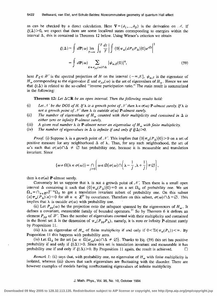
5422 Bellissard, van Elst, and Schulz-Baldes: Noncommutative geometry of quantum Hall effect
as can be checked by a direct calculation. Here V =(a, ,...,dD) is the derivation on .I%. If &A)>O, we expect that there are some localized states corresponding to energies within the interval A, this is contained in Theorem 12 below. Using Wiener’s criterion we obtain
t(A)= 1 dP(@)JTm I,‘: / 1 (O~~,(dP,P,)lO)erEz~z
= dP(w) I c I h,EcN14~
E~u~~(~)r-lh (59)
here P, E 3. is the spectral projection of H on the interval (-a,,!?], +,,E is the eigenstate of H, corresponding to the eigenvalue E and upp( w) is the set of eigenvalues of H, . Hence we see that &A) is related to the so-called “inverse participation ratio.” The main result is summarized in the following:
Theorem 12: Let ACR be an open interval. Then the following results hold:
(9 Let ,4 ^ be the DOS of H. If X is a growth point of M then X E a(o) P-almost surely. If X is not a growth point of .4” then X is outside o-(w) P-almost surely.
(ii) The number of eigenvalues of H, counted with their multiplicity and contained in A is either zero or in$inity P-almost surely.
(iii) A given real number X is P-almost never an eigenvalue of H, with finite multiplicity. (iv) The number of eigenvalues in A is infinite if and only tf &A)>O.
Proof (i) Suppose X is a growth point of .N. This implies that (0 Irr,( PA) IO) > 0 on a set of positive measure for any neighborhood A of h. Thus, for any such neighborhood, the set of o’s such that a(o) fIA # 0 has probability one, because it is measurable and translation invariant. Since
{wEf.-$iEu(O)}= n 1 wEalfl(ti)n h-i A+: #0 ,
j>O i i I
then ~E(T(o) P-almost surely. Conversely let us suppose that A is not a growth point of N. Then there is a small open
interval A containing it such that (01 7~,( PA) IO) = 0 on a set II0 of probability one. We set fi,=n n ,z~T-“CIo to get a translation invariant subset of probability one. On this subset (nl~dPA)b)=O f or all n E ZD by covariance. Therefore on this subset, c(o) nA=0. This implies that X is outside g(o) with probability one.
(ii) Let P,,(w) be the projection onto the subspace spanned by the eigenvectors of H,. It defines a covariant, measurable family of bounded operators.3’ So by Theorem 6 it defines an element P,, of %‘Y Thus the number of eigenvalues counted with their multiplicity and contained in the Bore1 set A is the dimension of rr,( P,,PA), namely, it is zero or infinity P-almost surely by Proposition 11.
(iii) Xis an eigenvalue of H, of finite multiplicity if and only if OCTr( rW(Ph))<m. By Proposition 11 this happens with probability zero.
(iv) Let a,,, be the set {w E !J] oppp( o) f7A # 0). Thanks to Eq. (59) this set has positive probability if and only if &A) >O. Since this set is translation invariant and measurable it has probability one if and only if &A) > 0. By Proposition 11 again, the result is achieved. El
Remark I: (ii) says that, with probability one, no eigenvalue of H, with finite multiplicity is isolated, whereas (iii) shows that such eigenvalues are fluctuating with the disorder. There are however examples of models having nonfluctuating eigenvalues of infinite multiplicity.
J. Math. Phys., Vol. 35, No. 10, October 1994
Downloaded 09 May 2005 to 128.32.113.135. Redistribution subject to AIP license or copyright, see http://jmp.aip.org/jmp/copyright.jsp

Bellissard, van Elst, and Schulz-Baldes: Noncommutative geometry of quantum Hall effect 5423
Remark 2: The criterion (iv) does not eliminate the occurrence of some continuous spectrum.
B. Noncommutative localization criterion and localization length
We introduce a second physical idea of localization: the average mean square displacement 6X( 7’). Let X be the position operator in G and X,(t) = erHwfXeVrHJ its time evolution. Then we consider:
K,,U-)2= I ,’ G (nlLL(t)-X)21n).
The covariance relation leads to 8X,,,(T) = c~X~-~~,~(Z’), so that it is sufficient to examine the behavior of the state IO). Averaging over the disorder and using again our algebra we get
SX( T)2= (60)
Boundedness of 8X(T) in time T will be an indicator for localization and behavior proportional to TV, LT E (0, l] will be interpreted as diffusive or ballistic quantum motion. In order to localize in energy we restrict the motion to energies in a Bore1 subset A of the real line and get &X,(T) in much the same way. On the other hand taking T -SW leads us to define the A-localization length as
E2(A)=lim sup T-m I
oT : mIv(e-(L’h) H’PA)12). (61)
Boundedness of 12(A) will be our localization condition for the spectral subset A.
Theorem 13: Suppose that 12(A)<w. Then H, has pure-point spectrum in A for almost every cs~fl. Moreoven zfM(E)=Y(Ps) is the density of states, there is a N-measurable fine- tion 1 on A such that for every Bore1 subset A’ of A:
12(A’)= I
A,dN(E)l(E)2. (62)
Finally, ifZ2(A)<m, 12(A’) is given by
12(A’)= I
dP(o) 2 lnl2 2 I(Ol~~(~~q)lnN2. (63) neZ2 E~uppp(w)nA’
Theorem 14: If the localization condition 12(A) < 00 is satisjed, then at every regularity point of the density of states, the application EE A-+PE E Y is continuous.
Remark I: Letting A shrink to one point E, the function 12(E) represents a kind of average of the entity ~Cne~4n121 +E.w(n>12p where $E,o is an eigenvector of H, corresponding to energy E; here the average is taken over the disorder and a small spectral set around E. This quantity measures the extension of this eigenstate. For this reason the function 1 will be called localization length for H. Note that no exponential decay of the wave functions is needed for our localization length to be finite. However, such behavior may be studied within the present framework; we postpone the details to future work.
J. Math. Phys., Vol. 35, No. 10, October 1994
Downloaded 09 May 2005 to 128.32.113.135. Redistribution subject to AIP license or copyright, see http://jmp.aip.org/jmp/copyright.jsp
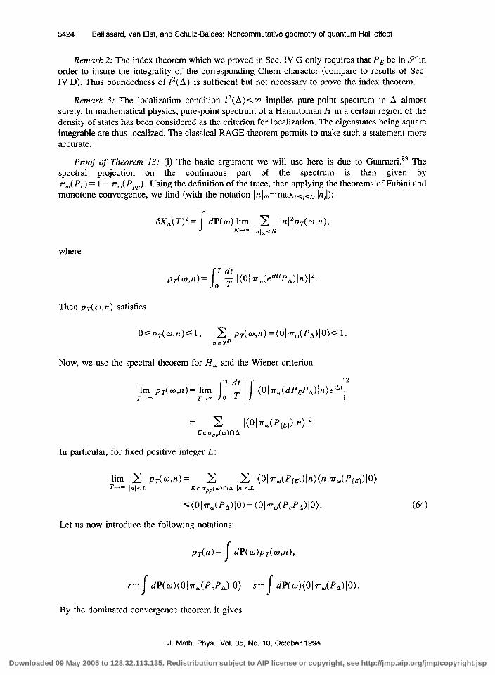
5424 Bellissard, van Elst, and Schulz-Baldes: Noncommutative geometry of quantum Hall effect
Remark 2: The index theorem which we proved in Sec. IV G only requires that P, be in Yin order to insure the integrality of the corresponding Chem character (compare to results of Sec. IV D). Thus boundedness of Z2(A) is sufficient but not necessary to prove the index theorem.
Remark 3: The localization condition Z2( A) <a implies pure-point spectrum in A almost surely. In mathematical physics, pure-point spectrum of a Hamiltonian H in a certain region of the density of states has been considered as the criterion for localization. The eigenstates being square integrable are thus localized. The classical RAGE-theorem permits to make such a statement more accurate.
Proof of Theorem 13: (i) The basic argument we will use here is due to Guameri.83 The spectral projection on the continuous part of the spectrum is then given by T,( P,) = 1 - T,( P,,) . Using the definition of the trace, then applying the theorems of Fubini and monotone convergence, we find (with the notation Inlm= maxl,i60 [nil):
EXAM= I dP(w);~m, & In12pT(w,n), n,<
where
PTtwn)’ I ,‘G I(olm,(e’H’PA)ln)12.
Then ~r( o,n) satisfies
Now, we use the spectral theorem for H, and the Wiener criterion
= c IwLJ(qE~)l~N2. E~r~~~(rn)nA
In particular, for fixed positive integer L:
lim 2 pr(w,n)’ T-+- Inl<~ c c (Ol~w(P{E})ln)(nl~o(P{E})IO)
EEO~~(UI)I-IA InlcL.
~(0l~~(PA)10)-(0l~,tP,PL\)IO).
Let us now introduce the following notations:
pTtn>= dP(m)PT(w,n)v I
r= I dP(w)(ol~~tPcPA)Io) s= dP(~)(Olmw(PA)IO)- s
(64)
By the dominated convergence theorem it gives
J. Math. Phys., Vol. 35, No. 10, October 1994
Downloaded 09 May 2005 to 128.32.113.135. Redistribution subject to AIP license or copyright, see http://jmp.aip.org/jmp/copyright.jsp
Bellissard, van Elst, and Schulz-Baldes: Noncommutative geometry of quantum Hall effect 5425
I dptw) 1h-l-l c PT( o,n)= lim 2 pT(n)Gs-r. T+,- Inl<~ T-m [,+a
Since r30, one can find T,>O such that, if TZ=T,, one has ClnlcL pr(n)ss-r/2. Thus, for TaT,:
Taking the lim sup over T we get Lrc12(A) for all L, implying that r= 0. Thus for almost ail o E a: (01 n,( P,PA) IO) = 0. Using the covariance relation and since ZD is countable, there is fk’Cfl of probability one such that (~~~,(P,P~)~~)=O for all nczZD. In particular 7rw(Pc)ln)=0 for all II E ZD and all w E a’, namely the continuous spectrum in A is empty.
(ii) Given two Bore1 subsets A r , A2C A, we define the following expression:
@$$(A, A21 = I oT f, zr. ln12(~lrrw(e’Hr~Al)l~)(ol~~(e~~~~~~)l~~.
n
This expression gives a Bore1 function in w. We use the Wiener criterion:
l~@&h,A,)=,~L InI2 c T--
l(01~,(P~,))ln)12=~~)(A~.A2). n E~cr~,,(w)nA~nA~
From this definition of 8’$( A ‘) for a Bore1 set A ’ CA it follows that
(a) O~~~‘(Ar)~L2(01rr,(Pp,P~,)ln)~~2; (b) if AttlA,=0, then 8$“(AIUA2)=@~)(At)-t8~)(A2); (c) $J)(A~)~@;+*)(A~>; (d) &:‘(A’) is a Bore1 function of o as pointwise limit of Bore1 functions; (e) if (Aj)jeN is a decreasing sequence of Bore1 subsets such that “jENAj=(ZI, then
am’ decreases to zero.
Averaging over the disorder, we obtain @)( A ’ ) = JdP( W) @L)( A ‘) which fulfills (a),(b),(c), and also (e) thanks to the dominated convergence theorem. Moreover, since @‘(A ‘) <L2, we can use the dominated convergence theorem, Fubini’s theorem, and the definition of 12(A) to get
dP(o) c ln121(0171-,(e’HfpA,)ln)12~z2(A’). InlQ
In much the same way, we get, thanks to (b), %@)(A’)==r2(A)<m,VIL E N. As ?@)(A’) is bounded and increasing in L, it follows that g(A ‘) = lim,,, @‘)( A ‘) exists. B defines a non- negative set function on the set of Bore1 subsets of A. Because of property (e), it is continuous from above and since it is moreover finite, we can conclude its a-additivity. Therefore B is a Radon measure. Moreover, using the monotone convergence theorem:
(iii) Let us show now 12( A ‘) < ?Y( A ’ ). Recall that
J. Math. Phys., Vol. 35, No. 10, October 1994 Downloaded 09 May 2005 to 128.32.113.135. Redistribution subject to AIP license or copyright, see http://jmp.aip.org/jmp/copyright.jsp
5426 Bellissard, van Elst, and Schulz-Baldes: Noncommutative geometry of quantum Hall effect
,%‘(A’)= 1 dP(@)~p, ,& ‘““;li= I,’ ~l(Ollr,(e’x’PA,)ln)12<~. E n
We can replace the limit by the lim sup. Hence for a fixed To large enough, the following expression is finite and we may apply Fubini’s theorem:
> lim sup f f T it dP(w) sup 2 ln)21(01~,(e'HrPA~)ln)12 TZT,, 0 T NEN Inlo
=Z2(A’).
As this is true for all To, we obtain Z2( A ’ ) s 27( A ’ ), and with (ii) their equality.
(iv) To finish the proof we use the Radon-Nikodym theorem. It is thus sufficient to show that the measure Z2(A’) = tF(A’) is absolutely continuous with respect to the density of states. Let A ’ C A be such that &‘(A’) =Y(PA,) = 0. From the definition of the trace it follows that (Ol%(PAr)lO)=O d most surely. By covariance and because ZD is countable, this gives T,(P~~)ln)=o for all n E ZD almost surely. Then the definition of gTfL(A ‘,A’) implies that it is zero for any Z,T and almost all w; consequently 0 = @A’) = Z2(A’). q
Let us give another useful expression for Z2(A). We consider finite partitions 9 of A into disjoint Borelian subsets:
~{AjCA,Aj Borelian I j=l...q,UiAi=A,AinAk=O}.
The set %(A) of such finite partitions is ordered by refinement
-9’ @ VA’EY~A”EP such that A’CA”.
This gives an ordered net. We define
i2(A)= lim ,)n= --(A) Az.F s(lvpAr12)9 (66)
where the limit is understood to be the one under refinements of partitions.
Proposition 12: f2(A) is well de$ned in R=RU{a}. Moreover:
i2(A)= SUP 2 flIvP,112). .A b(A) A' E.P
Proof: It is sufficient to show that refining the partition results in the increase of the quantity EA~E.~Y(lVPA~12). Take A=AtUA2,A,nAa=0, and suppose .T(IVPAI~)<~. We have
J. Math. Phys., Vol. 35, No. 10, October 1994
Downloaded 09 May 2005 to 128.32.113.135. Redistribution subject to AIP license or copyright, see http://jmp.aip.org/jmp/copyright.jsp

Bellissard, van Elst, and Schulz-Baldes: Noncommutative geometry of quantum Hall effect 5427
Now, either one of the Sobolev norms of PA, and PA, is infinite and in this case the inequality
~~;IVPA,UA,I~) J”TIV~‘A,UA~ ~2)~.T(~VP~,~2)+.QlVP~2~2) is trivially satisfied, or the com- ponents of VPA, and VPh2 are in L2(&,9’). The Hijlder inequality implies VPA,. VPA E L’ (&YJ . We may therefore treat each term separately.
2
We apply the cyclicity of 3and the formulas
PA,~I-PA 2, PA,< 1 -PA ,’ vpA2pA, = - PA2VPA,r
to get
The same calculation for the other term then implies the result. cl Because of Eq. (63), one expects i2 to be equal to Z2 and this is what we shall prove in the
sequel. We first need the following technical lemma:
Lemma 16: Let CL, v be two finite positive measures on a BoreZ subset A of the real line and PPP ‘VPP their pure-point parts. For a jinite partition 9’ of A we set
fltA,fl= 2 /-4A’)vtA’). A’GS
Then
lim -4TA,9= inf ~+‘I&3q= 2 ~ppt~~l)vpp(~~)). .A %(A) YE Z(A) EEA
Proof First, we show that JY( A,3 decreases as the partition is refined. We introduce F(a=UA,..A’XA’. Suppose that-q, t.hen.F(y)CF(a. As p@v is a finite positive measure on a Bore1 subset of R2, we have
Let us now consider the Lebesgue decomposition of the measures ,z and v in continuous and pure-point parts:
As the measures are finite, the continuous parts satisfy
VE>OEIS>O such that pJA’)<e, v,(A’)<&+A with diam(A’)<S.
Here, the diameter is defined by diam(A’) = SUP,,~ E A’, Ix-y j . Now we choose and fix a sequence of .Ya of finite partitions which satisfies:
lim( max diam(A’))=O. n-+m A’d,,
J. Math. Phys., Vol. 35, No. 10, October 1994
Downloaded 09 May 2005 to 128.32.113.135. Redistribution subject to AIP license or copyright, see http://jmp.aip.org/jmp/copyright.jsp
8428 Bellissard, van Elst, and Schulz-Baldes: Noncommutative geometry of quantum Hall effect
For such a sequence 9$ the following holds:
;ol ( U (A’XA’))={(X,.x)I.xEA}=Diag(AXA). *=’ A’d,,
In the limit, the contribution containing a continuous part vanishes for indeed for instance
lim k@Vpp( U n-m A’ E.f)n
(h’XA’))s)+te(n) 2 v,,(A’)~~+ie(n)v(A)=o, A’E.fn
Therefore, using the c+-additivity of the finite measure ~8 v (which is equivalent to continuity from above), we find
lim c ,4A’)v(A’)=;:? ,“, ~Lpp(A’)vpp(A’)=~pp~~pp( ; U (A’xA’)) n+- A’ E.7,)” ‘E ” ‘=’ A’E./‘”
=~pp@vppDiagtAXA)= c P~,<{E)>@v~~({E)). EEA
This is true for every such refining sequences of partitions, leading to the result.
Proposition 13: If Z2( A) <w, then Z2( A ‘) = i2(A ‘) for every Borelian subset A ’ CA.
Proof: As Z2(A)<m, Theorem 13 shows that
q
@)(A)= dpcO,,n~L bl2 c I(“lTdP{E})b)12. f EEuppp(0)nA
We decompose the complex measure ,U( A’)=(01 Tr,( PA,)ln) by polarization into four positive measures:
With these notations, we apply Lemma 16 to each term to get
f 4
@ ‘(A)= dV~lln~L InI 2 c pk@pk-2p1@‘LL2-2p3@p4 EEu&JO)nA k=l
= f dP(w) 2 lnl2 lim bl<L
,fa z(A,l ,z,, ~(0b~(PA~t)b>12.
The dominated convergence theorem now gives
&‘)(A) = lim ,,+d(A’} A& ’
dP(o) c In121(OIa,tPA~~)ln)12=~-L)tA),
Inl<L
by definition of sL)(A). Obviously we have
dP(o) $$ In121(01~,(pA,,)ln)12=i2(h’). tlEZ
J. Math. Phys., Vol. 35, No. 10, October 1994
Downloaded 09 May 2005 to 128.32.113.135. Redistribution subject to AIP license or copyright, see http://jmp.aip.org/jmp/copyright.jsp

Bellissard, van EM, and Schulz-Baldes: Noncommutative geometry of quantum Hall effect 5429
Moreover, %)( A ‘) is increasing in L. Since @)(A) is bounded by Z2(A), so is ,@‘(A). Its limit therefore exists. Actually, it converges to !*(A’). For indeed, with the dominated conver- gence theorem, we find
i2(A’)= sup =f
.PE .?(A’) A”E~
r
= SUP SUP c .A Z(A’) LEN A”E.&’ J dP(o),nzL lnt21(01~,(PA~~>l~>12
=f+li %‘(A’),
This finishes the proof. 1p
Proof of Theorem 14. Fix E,E’ E A,E<E’, then
cl
IIPE~ -pAI.“,= IP[E, Er]ll;- -=p([E, E’])+J%‘-(E’)-M-(E)
= I
E’(l(E”)2+ l)dJtr(E”). E
Now, in the limit E’+E, this is zero if E is a regularity point of ~9”. cl
C. Localization in physical models
In this section we give an example of a physical model for which the localization condition I’( A) < 03 is satisfied both for weak disorder at the band edges and for high disorder all over the spectrum. For the mathematical treatment we will, once again, restrict ourselves to the discrete case. Our line of arguments will use results of Aizenman and Molchanov.84*40 They give a simple proof of mathematical results proved earlier.35*85*38*31,37 We will conclude with some remarks about the continuous case.
As a preliminary, let us remark that if the spectrum has a finite gap A, then the condition 12(A)<m is satisfied for the simple reason that PA=O. In dimension two, the Chern character corresponding to every energy band is therefore an integer and the Hall conductivity an integer multiple of e2/h. However, this integer may be zero.
The analysis by Aizenman and Molchanov consists of two steps: first, one shows exponential decay of low moments of Green’s function for concrete classes of models and in specified regions A of the spectrum; then, this decay is useda to show exponential decay in In - m I of the quantity SdP(o)8upf,o(nl~(e’H’PA)lm). Th’ is, in turn, will allow us to show that Z2(A) <a is satisfied.
Here, we fix our attention to the D-dimensional Anderson model with constant magnetic field. The Hamiltonian acting on &ZD) is given by
H o,h=Ho+XV,, XER,
where H,, is the D-dimensional analog of Hamiltonian given in Eq. (10). V, is the disorder potential: at every site of the lattice it takes a random value in the interval [ - 1, 11; the probability distribution is supposed to be uniform and the sites are independent. In Refs. 40 and 84 much more general situations are considered: the kinetic part H,, may have nonzero elements farther off the diagonal as long as they decay exponentially in distance from the diagonal; the random potential may also have gaussian or Cauchy distribution; moreover, correlations between the sites are allowed in a sense to be made precise. For us, however, the Anderson model captures the essential of the localization phenomenon and it has the advantage that the hull (fi,T,P) is easily
J. Math. Phys., Vol. 35, No. IO, October 1994
Downloaded 09 May 2005 to 128.32.113.135. Redistribution subject to AIP license or copyright, see http://jmp.aip.org/jmp/copyright.jsp

5430 Bellissard, van Elst, and Schulz-Baldes: Noncommutative geometry of quantum Hall effect
constructed as topological product of intervals [ - 1, 11; by Tychonow’s theorem, s1 is compact; the action T on !2 is given by the translations in physical space and the product measure of the uniform probability on [ - 1, l] is a T-invariant and ergodic measure P on R.
We will now describe precisely in which situations Aizenman and Molchanov prove expo- nential decay of low moments of Green’s functions for the Anderson model:
1 dP(o)i(nln,i &-JIm)~s4De-cln-mi, sE(O,l).
The first situation is that of strong disorder: for every s E (0,l) there exists an h,= X,(D,s) such that for Xa‘x, the bound holds on all of the spectral axis.
The second situation considers weak disorder, that is small X. Recall that the free Hamiltonian Ho has energy bands of continuous spectrum. In the interesting case for us of dimension two, the energy bands and their dependence on the magnetic field are given by Hofstadter’s butterfly; Ho then gives Harper’s equation. For the Anderson model the bound (67) is obtained for energies E situated at band edges:
EER(X)= U {EER-~(H~)~~A~,(E)<~}, ss(O,l)
where
g,(E)= sup ( ED I(n]rw( &)im)lS)-‘. XEZD YEZ
[For the Anderson model, the constant K(S) appearing in Ref. 84 is equal to i independent of s.] By a Combes-Thomas argument, one get.? the asymptotic behavior of g,(E) in t=dist (E,a(Ho)):
- ,p+Dw, 5-0
g,(E) = * e+m
Therefore, because a(Hk)C{EIE E {a(H,)+ } Y ; r&h}, the intersection of R(X) with (T(H~) is nonempty for X sufficiently big. In other words, the bound (67) is satisfied for some energies belonging to the spectrum and situated at the band edges. This is probably the case as soon as A # 0; dimension two is critical.28
Let us now come to the second step of Aizenman’s analysis. If the bound (67) is satisfied for an interval A of the spectral axis, he proves that the unitary evolution operator filtered with the spectral projection PA satisfies:
I dP(w)~~~j(nlrr,(P~etHr)lm)l~Ce-DI”-”’, C,DER+.
Let us now use this result to show that the noncommutative localization condition is satisfied. Because II ?r,( Ppe’Ht)]] ZcKZzD)S 1, we have
J. Math. Phys., Vol. 35, No. 10, October 1994
Downloaded 09 May 2005 to 128.32.113.135. Redistribution subject to AIP license or copyright, see http://jmp.aip.org/jmp/copyright.jsp
Bellissard, van Elst, and Schulz-Baldes: Noncommutative geometry of quantum Hall effect 5431
Now, taking the time-average we see that 12(A) <m. This is, of course, only true if either X>h, or ACR(h).
Let us now comment on the case of continuous physical space. First of all, if the Fermi energy EF lies in a finite gap, then it can be shown that PF E 9 86 For strong disorder, one expects a finite localization length, but near the set {h w,( n + i) I o, = e-S/m, n E Z} the localization length prob- ably diverges. This would be the analog of the discrete case.
VI. APPLICATIONS AND COMPLEMENTS
A. Low-lying states do not contribute to the IQHE
In this section, we address the following question: consider the Landau Hamiltonian HL and add a periodic potential VP of varying strength
H=HL+uVp, 0~V,sl.
How do the Chem numbers evolve as the coupling parameter (T is increased? In particular, what happens if a% fiw,?
Halperin et aLg7 made corresponding numerical calculations. They took a finite size sample and computed the Chem numbers for various values of u by the method described in Sec. VI C. For small (T, the weak periodic potential approximation is valid and the Chem numbers are those given by the Diophantine equation (70). For intermediate values of (+, the energy bands cross each other in a complicated way and it is difficult to follow the Chem numbers. However, for a4h W, , Halperin et al. observed the following striking result: all low energy bands of the spectrum carry zero Hall current. This result was put on a rigorous basis by Nakamura and one of the authors.86
Theorem 15: Consider the Hamiltonian H= HL+ crV where V is a potential satisfying the conditions below. Then for u sufficiently large the spectrum has gaps between his low energy bands (energy smaller than eh w, , where E appears in the conditions below). If the Fermi energy lies in one of these gaps, the Hall conductivity vanishes.
Hypothesis on the potential V:
xER2 v(x)=o, supxER2 v(x)~c<w. Ii?) g ere is a countable set of R2,{xn,n=1,2,...} such that Ix,--X,[>d if n # m with
d>O. (iii) There are e>O and PEC~(BJ where B,={xER~IIxI<E} such that d>2e and
V(x,+x) = W(x) for x E B, and for all n, (iv) 0 is the unique nondegenerate minimum of !YE B,. (v) If Ix,--xI>E for all n, then V(x)3S>O.
Note that this potential is not strictly periodic, although the bottoms of the wells need to be identical. The framework of the proof is that of noncommutative geometry completed by semi- classical analysis. Let us just describe the strategy here. The existence of the gaps follows from semiclassical analysis: the energy levels of a single, isolated quantum well are enlarged by the tunneling effect; the band width can be estimated by eeaG’,,>O. In order to show that the Chem character is zero, one proceeds as follows. First consider the situation of quantum wells separated
J. Math. Phys., Vol. 35, No. 10, October 1994 Downloaded 09 May 2005 to 128.32.113.135. Redistribution subject to AIP license or copyright, see http://jmp.aip.org/jmp/copyright.jsp
5432 Bellissard, van Elst, and Schulz-Baldes: Noncommutative geometry of quantum Hall effect
by infinitely high barriers. The projection Pi on the energy level of quantum well number j is one-dimensional. Its Chern character therefore vanishes. Now we consider the projection P, = @ iPi, where the sum runs over all wells. Because of the additivity of the Chern character (compare Lemma 12), the Chern character of P, is zero as well. Finally, semiclassical analysis allows us to show that P, is Murray-von Neumann equivalent to the projection PE onto the energy band which arises as the barriers are reduced to finite height. In view of Lemma 11, this finishes the proof. It is likely that the result also holds if the projection is not in the gaps.
B. Where and how does the localization length diverge?
In this section, we review the most important results on the behavior of the localization length at the center of the broadened Landau level. Discussion of theoretical ideas is followed by a brief presentation of numerical techniques and results. As before, we consider a system of independent fermions in a disorder potential described by a one-particle Hamiltonian.
In numerical calculations and scaling theory, a rather strong notion of localization is often used, that of a Lyapunov exponent X(E). If one supposes exponential decay of the correlation function of the wave function flE corresponding to the energy E, X(E) is defined by
Here the average is taken over disorder configurations. Physicists often call the inverse of X(E) the localization length. However, except for in the one-dimensional case, there is yet no clear mathematical formulation.
In 1979, the gang of fou?’ used scaling theory (ideas due to Thouless 4*) and renormalization group calculations to show that, at absence of magnetic field, two is the critical dimension for localization in the following sense: for dimension smaller than two, all states are exponentially localized at any strength of disorder, that is, for all wave functions there are positive Lyapunov exponents. For dimension greater than two, there exist extended states for low disorder. At dimen- sion two, all states are localized except for states corresponding to isolated critical energies at which the localization length diverges. In the case of perpendicular magnetic field in two dimen- sion, the same result holds as shows a development of higher order.42
In the QHE, the Hall conductivity does not vanish. This led Halperin to postulate the existence of extended states.” A corollary of Theorem 1 is the following:
Corollary 13:13 Between different plateaux, there has to be a spectral interval A such that the localization condition 12(A) <~a is violated.
Remark that the interval may be very small. It is even likely that there is, in fact, a single energy E such that PsE is not in the Sobolev space Y. This implies, of course, 12(A) = C=J for every interval containing E. Corresponding numerical results are presented at the end of this section.
We now come to the question of how the localization length diverges. If one considers a disorder potential varying on a length scale much bigger than the magnetic length, the motion can semiiclassically (in the magnetic field) be well approximated by a motion along equipotentials of the disorder potential. Percolation theory now indicates that there is one critical energy E, to which correspond extended states. Moreover, at this energy the localization length diverges as
& E/E-E,[-~.
Trugman evaluated V= $,88 but more thorough examination of the effect of tunneling between the wells and mountains led Mil’nikov and Sokolov to predict ~=f.~~ In spite of the simplicity of
J. Math. Phys., Vol. 35, No. IO, October 1994
Downloaded 09 May 2005 to 128.32.113.135. Redistribution subject to AIP license or copyright, see http://jmp.aip.org/jmp/copyright.jsp

Bellissard, van Elst, and Schulz-Baldes: Noncommutative geometry of quantum Hall effect 5433
the theoretical approach, the agreement with numerical results obtained by three different methods is very good. These latter are the Thouless number method, the Chem number method and the third one is a scaling theory approach; the original ideas behind are due to Refs. 90,91,43, and 44, respectively.
The Thouless number method is the most elementary because only energies and no eigenvec- tors need to be calculated. In the interesting case of strong magnetic field, calculations were made by Ando. The Chem number method93 is described in some more detail in the next section. Let us concentrate on the scaling theory approach. One considers a cylinder of (small) circumference M and extended to infinity in one direction (denoted by the variable z). The magnetic field is perpendicular to the cylinder surface. Choosing the Landau gauge A = (O,O,%‘z), the eigenstates of the free Hamiltonian are centered on circles around the cylinder corresponding to fixed values of L. This discrete set of eigenstates will serve as base for the Hilbert space; in this base one also expresses Hamiltonian perturbed by disorder. Now for fixed circumference and fixed energy, one calculates numerically the disorder averaged Lyapunov exponent LM of a ‘wave function by the transfer matrix method. Finite size scaling theory43 then allows to estimate the behavior of the localization length near the critical energy; in particular, the exponent v in Eq. (69) can be calculated. In presence of magnetic field, this method was first used in Refs. 45 and 48; more recent and more extended numerical studies46Y94 confirm the theoretical prediction V= 5. It seems that the exponent is independent of the disorder distribution and the Landau level index (if the Landau level interaction are taken into account).
What is the behavior of the wave function at the critical energy E, itself? Pichard and Sarma43 suggest the following in order to calculate the exponent x for the powerlaw decay of the wave function I+?~~:
One calculates as before the Lyapunov exponent LM for different M at fixed energy E, . With the hypothesis of conformal invariance, x can then be shown to be equal to the slope of the linear relation between h4 and l/L,. Chalker and Coddington95 estimate x-0.27. We remark that this implies that the weak localization condition PsE,~ 7 is violated. Therefore, at critical energies (that is at the centers of the broadened Landau levels) the Chem number may change.
C. Chern numbers and localization in Harper’s equation
The Chem characters or Chem numbers of the energy bands of Harper’s equation correspond- ing to rational flux have already been computed by Thouless, Kohmoto, Nightingale, and den Nijs;8 we gave some insight in Sec. II F. Ando96*92 and more recently Tan97 have made numerical studies on the influence of an added disorder potential on these Chem numbers. We describe some of the results because they constitute a good illustration of theoretical ideas.
Let us first recall that Harper’s equation (11) is obtained in two different limiting cases. One consists in adding a weak periodic potential V,, to the Landau Hamiltonian HL, for example, a two-dimensional sinusoide; projecting H,+ VP on a subspace corresponding to one Landau level then leads to Harper’s equation. On the other hand, if one adds a strong periodic potential (which means that its well is much deeper than fi oc), the low energy region of the spectrum is well described by a tight binding model [Eq. (lo)]. As shown in Sec. II F, Bloch’s representation also leads to Harper’s equation.
The spectrum of Harper’s equation is well known and its dependence on the magnetic flux per unit area 4 is represented in Hofstadter’s butterfly.99 The parameter a appearing in EQ. (11) is proportional to 4 in the tight-binding case and proportional to the inverse of 4 in the case of weak periodic potential. Let us now suppose the rationality of a=q/p, where p and q are relatively prime integers. The spectrum then consists of p energy bands of extended states. The Chem
J. Math. Phys., Vol. 35, No. IO, October 1994 Downloaded 09 May 2005 to 128.32.113.135. Redistribution subject to AIP license or copyright, see http://jmp.aip.org/jmp/copyright.jsp

5434 Bellissarci, van Elst, and Schulz-Baldes: Noncommutative geometry of quantum Hall effect
number of the rth band can be calculated with the Diophantine equation in the following way.8T’oo There exist unique integers s, ,t, (except for even p and r=p/2) such that Is,1 ~p/2 and satisfying
s,q+t,p=r r=O,...,p. (70)
The Chem number of the rth band and therefore its contribution in units of e2/h to the Hall conductance is given by I,- I,-, in the weak periodic potential case and by s,---s,.- 1 for the tight-binding model. Remark that as to= 0 and tp= 1, the sum of all p Chem numbers in the weak periodic potential limit is equal to one. This reflects the fact that the bands result from the splitting of one Landau level with Chem number 1. On the other hand, so = sP = 0, such that the sum of the Chem numbers in the tight binding approximation is zero.
Now a disorder potential will be added. This could be, for example, an Anderson-type per- turbation (compare Sec. V C), but in the numerical simulations a densely distributed potential with two values Vd , - V, was used. The fractal structure of Hofstadter’s butterfly disappears as soon as disorder is turned on. Because many gaps close, it becomes possible to label the remaining energy bands by a finite number of rationals for any (maybe nonrational) parameter (Y. What are the Chem numbers of the bands and how do they evolve as a function of the disorder strength?
Before starting the discussion, let us comment on the physical relevancy of the two approxi- mations. In the usual QHE samples presented in Sec. II B, neither seems to describe the reality: the disorder potential is much stronger than the weak periodic potential due to the ions within the surface. On the other hand, because the mobility is very high, the tight-binding approximation is not appropriate. However, lately so-called antidot superlatices seem to open the possibility of the experimental realization of parts of Hofstadter’s spectrum (of course, only in a very approximative way). In these systems the ideas we present here could be tested.
For all details on how the numerical results were obtained, we refer to the original works?6*97 but let us describe the principal steps. Of course, the calculations are made in finite size samples and therefore disorder is just treated in an increased unit cell, causing thus a splitting of the Harper
Disorder
2 -3 2 Energy
FIG. 5. Suggested phase diagram for the weak potential approximation.
J. Math. Phys., Vol. 35, No. 10, October 1994
Downloaded 09 May 2005 to 128.32.113.135. Redistribution subject to AIP license or copyright, see http://jmp.aip.org/jmp/copyright.jsp
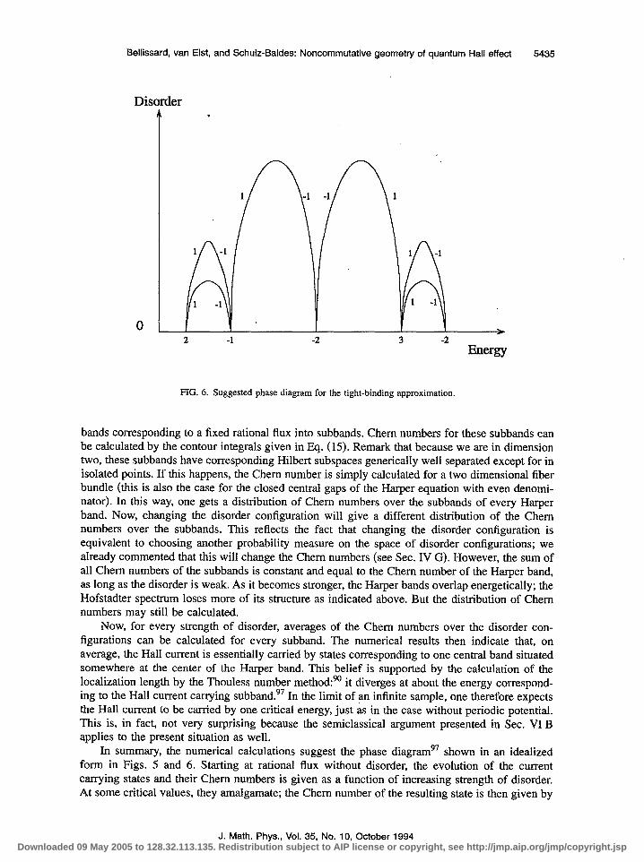
Belllssard, van Elst, and Schulz-Baldes: Noncommutative geometry of quantum Hall effect 5435
Disorder a ’
2 -1 -2 3 -2 Energy
FIG. 6. Suggested phase diagram for the tight-binding approximation.
bands corresponding to a fixed rational flux into subbands. Chem numbers for these subbands can be calculated by the contour integrals given in Eq. (15). Remark that because we are in dimension two, these subbands have corresponding Hilbert subspaces generically well separated except for in isolated points. If this happens, the Chem number is simply calculated for a two dimensional fiber bundle (this is also the case for the closed central gaps of the Harper equation with even denomi- nator). In this way, one gets a distribution of Chem numbers over the subbands of every Harper band. Now, changing the disorder configuration will give a different distribution of the Chem numbers over the subbands. This reflects the fact that changing the disorder configuration is equivalent to choosing another probability measure on the space of disorder configurations; we already commented that this will change the Chem numbers (see Sec. IV G). However, the sum of all Chem numbers of the subbands is constant and equal to the Chem number of the Harper band, as long as the disorder is weak. As it becomes stronger, the Harper bands overlap energetically; the Hofstadter spectrum loses more of its structure as indicated above. But the distribution of Chem numbers may still be calculated.
Now, for every strength of disorder, averages of the Chem numbers over the disorder con- figurations can be calculated for every subband. The numerical results then indicate that, on average, the Hall current is essentially carried by states corresponding to one central band situated somewhere at the center of the Harper band. This belief is supported by the calculation of the localization length by the Thouless number method:90 ing to the Hall current carrying subband.
it diverges at about the energy correspond- In the limit of an infinite sample, one therefore expects
the Hall current to be carried by one critical energy, just as in the case without periodic potential. This is, in fact, not very surprising because the semiclassical argument presented in Sec. VI B applies to the present situation as well.
In summary, the numerical calculations suggest the phase diagram97 shown in an idealized form in Figs. 5 and 6. Starting at rational flux without disorder, the evolution of the current carrying states and their Chem numbers is given as a function of increasing strength of disorder. At some critical values, they amalgamate; the Chem number of the resulting state is then given by
J. Math. Phys., Vol. 35, No. 10, October 1994 Downloaded 09 May 2005 to 128.32.113.135. Redistribution subject to AIP license or copyright, see http://jmp.aip.org/jmp/copyright.jsp

5436 Bellissard, van Elst, and Schulz-Baldes: Noncommutative geometry of quantum Hall effect
the sum of the merging ones (this sum may also be zero, Hall currents then annihilate each other). To conclude, let us comment on the limiting behavior for strong disorder. In the weak periodic potential approximation, one eventually obtains a Chem number one as for the Landau level. It is an interesting question what happens to the Chem number as the quantum Hall regime breaks down, certainly the corrections to the Kubo formula will be important at very high disorder. In the tight binding approximation, the system evolves to zero Hall current, this reflects the results of Sec. VI A.
VII. INTRODUCTION TO THE FQHE
A. Overview
While in 1982 Thouless, Kohmoto, Nightingale, and den Nijs made an important step towards the understanding of the IQHE,* Tsui, Stormer, and Gossard from Bell Laboratories made the surprising discovery that plateaux of the Hall conductivity could be observed not only at integer, but also at fractional multiples of e2/h. lo1 Using a high-quality GaAs-Al,Ga,-,As heterojunc- tion, they observed a plateaux at cHl( e2/h) = {. The corresponding minimum of the direct resis- tance was also observed. The filling factor was varied by changing the magnetic field while keeping the charge-carrier density fixed. In order to obtain the filling factor v= 4, they needed a magnetic field strength of about 1.5 T. The experiment was undertaken at different values of temperature (0.48, 1 .OO, 1.65, and 4.15 K) and even at the lowest of them, the accuracy of oH on the plateau was much more modest than in the integer effect.
Since this first experiment, the FQHE has been observed for many values of oH. The most striking results are the following:
(1) Let cHl(e2/h)=plq with p,q relatively prime integers. Then, q is odd (‘odd-denominator rule’). Recently, some deviations of this rule have been observed, but this seems to correspond to non spin-polarized electrons. In the sequence, we will not consider this case.
(2) The observation of the fractional effect requires very clean samples. It is easily destroyed by impurities causing inelastic scattering. Moreover, the stability of the plateaux with respect to temperature and impurity effects is very dissimilar for different fractions. In general, fractions with small denominator seem to be more stable. Thus, the plateaux appear in a well-defined order when lowering the temperature. This gives rise to series of fractions, also called ‘hier- archy of states.’
(3) In all devices, the accuracy of the Hall conductivity on the plateaux is much less for fractional than for integer values. Whereas in the IQHE we have &H/o,= 10m7, this is about 10m5 at best for the FQHE.
Although we have given a rigorous explanation of the IQHE, the situation is much less satisfactory for the FQHE. The QHE contains two distinct aspects: the existence of plateaux (which, for the IQHE, follows from localization of the states at the Fermi edge) and the integrality (respectively fractionality) of the Hall conductivity on them (which has a topological origin). Usually, these two points are not well separated in the literature on the FQHE. In fact, there are conceptual difficulties in understanding the role of localization in the case of interacting electrons. The mechanism which gives rise to the existence of plateaux is quite unclear. The main problem is that no useful Kubo formula is known to calculate the Hall conductivity for interacting Fermions. Instead, one usually follows another strategy: since we know that noninteracting electrons only exhibit an IQHE, it is clear that the FQHE might appear when electron-electron interaction can no longer be neglected. It is generally believed that at certain values of the filling factor, the ground state becomes incompressible owing to the repulsive two-particle interaction. Thus one tries to find explicit ground states which exhibit a fractional Hall conductivity. Then arguments are given to explain that this value remains constant while the filling factor is slightly changed. The most promising states that have been found show a remarkable property: they exhibit particlelike excitations with
J. Math. Phys., Vol. 35, No. 10, October 1994
Downloaded 09 May 2005 to 128.32.113.135. Redistribution subject to AIP license or copyright, see http://jmp.aip.org/jmp/copyright.jsp

Bellissard, van Elst, and Schulz-Baldes: Noncommutative geometry of quantum Hall effect 5437
some charge q # - e. The states are only defined for specific values of the filling factor, but it seems that the existence of quasiparticles is stable against perturbations if q/e is a fractional number. Apart from numerical evidence, there is no serious explanation of this property. The stability of quasiparticles is due to an energy gap separating the ground state from the excitations. It is conceptually not clear why the existence of such a gap is related to the fractionality of the quasiparticle charge. No rigorous results are known here.
B. Laughlin’s ansatz for the v= 1 lm ground state
Up to now, most attempts to explain the FQI-IEG-in particular the classical hierarchy of Haldane and Halperin102~103 as well as Jain’s composite-fermions approach’04-are based on Laughlin’s wave functions which describe a finite number of electrons in a finite volume, yielding a filling factor V= l/m with m an odd integer. In the following, we will review the ideas which led Laughlin to his proposal. Following Haldane, we will then construct a class of Hamiltonians for which Laughlin’s states are exact ground states.
Before doing this, we want to clarify the role of these states and try to justify our interest in them. As we have already mentioned, there does not exist a satisfying theory of the FQHE at the moment. In particular, the universality of the effect and its insensitivity to the exact form of the Hamiltonian is not quite clear. The main advantage of our approach to the IQHE is that we do not need to know the exact form of the one-particle potential, but only have to impose some mild conditions on it. To explain the existence of plateaux and to prove the integrality of (+H/( e2/h), we did not need to calculate the ground state explicitly. In our opinion, despite the wide use of Laughlin’s wave functions in the literature, the explicit form of the ground state does not lie at the heart of the theory, neither for the integer nor for the fractional effect.
Nevertheless, in our theory of the IQHE we were not able to give the explicit values of the Hall conductivity just by means of general considerations. In fact, the value given by the Kubo- Chem formula might depend on the choice of the probability measure P on the hull of the one-particle Hamiltonian. To derive the ‘right’ values, we computed explicitly the Chem character of the eigenprojections of the Landau Hamiltonian. A homotopy argument then shows that these values remain constant when the disorder is switched on, at least for small values of the potential.
The states which arise from Laughlin’s wave functions in the thermodynamical limit might play the same r6le for interacting particles: They yield the explicit values of the conductivity for a Hamiltonian with a restricted two-particle interaction and without one-particle potential. The main task which remains is to show that these values stay constant as the Hamiltonian is deformed continuously. This is going beyond the scope of our article.
We will now come to the description of Laughlin’s states. The general Hamiltonian for N electrons is given by
j=l
where in our case VXA(x) =3’ez, .9=const. Thus we assume that the two-particle interaction depends only on the distance between the particles. Under certain conditions on the functions U and V, HN is essentially self-adjoint on Cr(R2N). Furthermore, the N-Fermion space A NL2(R2) is an invariant subspace. Choosing suitable boundary conditions (we will choose Dirichlet boundary conditions on the disk AR = {x E R2: 1x1 CR}) yields a self-adjoint operator HN,Ain the N-fold tensorproduct gNL2(h). We will denote its restriction to A NL2(A) by the same symbol. Since the Laughlin states should play the same role for interacting electrons as the ground state of the Landau-Hamiltonian does for noninteracting ones, we will set V=O. In fact, up to now it is unclear what happens when the one-particle interaction is switched on, even for small values of the potential. The basic idea which leads to Laughlin’s states is the following: for
J. Math. Phys., Vol. 35, No. 10, October 1994 Downloaded 09 May 2005 to 128.32.113.135. Redistribution subject to AIP license or copyright, see http://jmp.aip.org/jmp/copyright.jsp

5438 Bellissard, van Elst, and Schulz-Baldes: Noncommutative geometry of quantum Hall effect
a strong magnetic field, the two-particle interaction can be treated perturbatively; if we start from a system of noninteracting electrons in the lowest Landau level, the excitations to higher Landau levels in the perturbation series can be neglected. Thus, for filling factors v< 1, we assume the ground state to be a linear combination of Slater determinants of one-particle wave functions belonging to the lowest Landau level.
For V=O, the remaining operator HN is rotationally invariant. Thus, we can look for joint eigenvectors of energy and total angular momentum. It is clear that, for a repulsive two-particle interaction, the particles will escape to infinity when not restricted to a finite volume. Classically, the trajectory of an electron in a constant magnetic field with angular momentum I and energy E is a circle around the origin with radius R = d=. Thus, for E = fL wJ2, restricting the particles to a disk with radius R is essentially equivalent to restricting the angular momentum to values less or equal than m&w,R2/2 = R2fL/2/,& = NfLlv= N& (with $A the magnetic length). Thus, in- stead of calculating the ground state of HN,n,, we are looking for an eigenstate of HN built of lowest Landau level wave functions with maximal angular momentum N,.r,. Laughlin, strongly influenced by the theory of liquid 3He, proposed the ansatz
ccl(Zl ,-.a, ZN)= ]iI g(zk-zj) ISj<kSN
for the N-particle ground state. Here and in the following, we set the magnetic length to unit and we use complex coordinates z =x+ zy in the plane. The lowest Landau level is spanned by the functions ~m~zme-(“2)lz12, thus
with an analytic function f. Since $ should be anti-symmetric under particle exchange, we have f( - z) = -f(z). Furthermore, as we are looking for eigenstates of total angular momentum M and the operator of angular momentum for one particle is given by zd, - ?a~, the product in the above formula has to be a polynomial of degree M in each variable zj. From this, it follows that f(z>=z" with an odd integer m. We will denote the resulting normalized wave function by ICrN,,, . The total angular momentum is M = [N(N - 1)/2]m and the particles are essentially re- stricted to a disk with radius R= J2m(N-1) (in units of the magnetic length) or, equivalently, v- llm.
Before we investigate the question for which Hamiltonians Laughlin’s ansatz yields an exact groundstate, we want to make some remarks on the tbermodynarnical limit. The QHE (the integer as well as the fractional) is assumed to be exact in the case of infinite volume and zero tempera- ture, thus necessarily we have to involve statistical mechanics. Laughlin’s states are states for a finite number of particles in a finite volume, i.e., we are working in the canonical ensemble. The Gibbs states are
(+,N,A= z;;-z;;’ I
where a is a bounded linear operator in A NL2( A). At zero temperature, they reduce to the vector states
(4 m,N,A=(@N,A 9atiN,A)j
where 9N.A is the (nondegenerate) ground state of HN,* . To investigate the limit N-+w, A-+R2 with fixed particle density N/IA], we have to include vector states with an arbitrary
J. Math. Phys., Vol. 35, No. IO, October 1994
Downloaded 09 May 2005 to 128.32.113.135. Redistribution subject to AIP license or copyright, see http://jmp.aip.org/jmp/copyright.jsp

Bellissard, van Elst, and Schulz-Baldes: Noncommutative geometry of quantum Hall effect 5439
number of particles, i.e., we have to work in Fock space. The algebra of observables should be a suitable subalgebra of bounded linear operators in this space. We will choose the canonical anti- commutation relations (CAR) algebra. We recall the definition: Let
F-(L2(R2)): = iti ANL2(R2) N=O
denote the Fermi-Fock space. For q5 E L2(R2) and $IE @ NL2(R2), we shall now define a*( q5)(//: = m#G3 t,li. Let P! denote the projection onto A NL2(R2) in BNL2(R2), i.e.,
1 p”~@-@~N=~ c (-)%%(l)@.**@h(N)r
‘U’S)J
where the sum runs over all permutations of (l,..., N). Let a*-(4)=P?la*(c$)P! on A NL2(R2), hence, for Cc, E ANL2(R2)
where ij denotes that the jth variable has to be omitted. This yields a bounded linear operator a?(+) in F-(L2(R2)) with ~~a*_(q5)~~=~~~~l. The adjoint operator is given by
a-(~>~(zl,...,z,-,>=\liS I R2d2Z &)$(Z,z~,...,z~-1)
for $IE A NL2( R2). These operators satisfy the CAR
The CAR algebra over L2(R2), which we will denote by A, is the C*-algebra of bounded linear operators in 9--(L2(R2)) generated by the identity and the set of operators {a -( 4): 4 E L2(R2)}.
We regard a state as a linear mapping (. )from this algebra into the complex numbers such that @*A)>0 VAE,&and(l)=l.Civenasequence($N)NENofvectors$NE ANL2(R2),wecan ask for the limit of the corresponding vector states. Here, the limit has to be understood in the Weak-*-tOpOlOgy, i.e., (.)=limN,, (.),v if and Ody if (A)=limN,, (A)N VA EA. It iS Clear
that the limit is not a vector state. As an example, we will treat the case m = 1. Then, Laughlin’s wave function is a single Slater
determinant (namely, Vandermonde’s determinant). The normalized wave functions are
#N.l(z, ,...,ZN) =
We will denote the limit state by ( .)m,l. It is completely determined once the correlation functions (UT=, a*_(+jj>n;=, a-(@k)> m,l are known. Obviously, these vanish for m # n. We will calculate the two-point function explicitly: We have (a i ( +)a - ( $)).Q = ( +, T4), where the integral kernel of T is given by
J. Math. Phys., Vol. 35, No. 10, October 1994 Downloaded 09 May 2005 to 128.32.113.135. Redistribution subject to AIP license or copyright, see http://jmp.aip.org/jmp/copyright.jsp

5440 Bellissard, van Elst, and Schulz-Baldes: Noncommutative geometry of quantum Hall effect
N-1 (22’/2)j 1 1/4(1zI*+Iz'1*) c -=- ,-(1/4)h'~*+W2) zAz'
j=O j! 2~
Thus, the operator T is just the projection onto the lowest Landau level. As a consequence, we get the correct filling factor V= 1. Furthermore, it can be shown that ( ~)~,t is a quasi-free state, i.e., the 2n-point functions are certain sums over products of two-point functions, for example (u*<~l>a*(~z)a-(~lll)a-((CI2))rn,l = (a*_(~l)a-(~,l)),,l(u~(~2)u-(~2))ffi,* - (a:(+&-
x W2>)co,,(~~ W2>~-Wl>)m,*; see Ref. 105 for an exact definition. But this is just the limit Gibbs state (for temperature T= 0 and filling factor Y= 1) for noninteracting electrons in a con- stant magnetic field. Thus in the thermodynamical limit we get the exact ground state.
This can also be seen from the work of HaldanelM which we will now review. Let II denote the projection onto the lowest Landau level in the one-particle space. We will investigate the Hamiltonian HN,eff: = IIeNHJI oN . The kinetic part just equals Nfi o/2. In order to calculate the integral kernel of II @ II U( Izj - .Q])II 8 II, we perform the unitary transformation
Then,
~(~~n)U(lZj-Z~l)(~~~)'~-l=n~(~U(lZj~l)n).
Since V(lzjkl) is rotationally invariant, the second factor in the tensor product is diagonalized by the simultaneous eigenstates of the Landau Hamiltonian and angular momentum. In this basis,
(~~~~(I~jkI)~mf)=UmSm,m’ with
2mfl
U(r),
where we have reintroduced the magnetic length G8. Thus, in some sense, the projection onto the lowest Landau level yields a ‘quantization of interparticle separation.’ For example, for the Cou- lomb interaction U(r) = e2/4 rrr we have
e2 r(m+ l/2) u”=G 2m! ’
For m+m, this falls off as l/v& . It is remarkable that the coefficients (I,,, are independent of f ’ .n exactly for the Coulomb interaction.
As a result, we state: The set of functions
with M,m E {0,1,2,...} forms a basis of eigenfunctions of II@IIU(lzj-zkl)IT@II. Each eigen- value U, is infinitely degenerate (according to an arbitrary angular momentum of the center-of mass motion).
J. Math. Phys., Vol. 35, No. 10, October 1994
Downloaded 09 May 2005 to 128.32.113.135. Redistribution subject to AIP license or copyright, see http://jmp.aip.org/jmp/copyright.jsp

Bellissard, van Elst, and Schulz-Baldes: Noncommutative geometry of quantum Hall effect 5441
The general two-particle wave function in the lowest Landau level with angular momentum maximal equal to NQ is given by
where PNa is a polynomial of degree Na in each of its variables. These states form a (p)-dimensional subspace, but this subspace is not invariant under the two-particle interaction. Let us assume that the sequence U, decreases monotonically. Then the desired ground state would be a state with relative angular momentum N *, or, since we are dealing with Fermions and therefore the relative angular momentum has to be odd, N+- 1. In the latter case, we have a degenerate ground state since we can choose A4 = 0 or A4 = 1. Let us remark that these functions are not equal to Laughlin’s ansatz for N= 2.
In the case of more than two particles, it is in general not possible to give the ground state. The general N-particle wave function in the lowest Landau level with maximal angular momen- tum equal to N@ is given by
ti(Zl ,-, zN)=PN+(zl ,..., zN)e-(1’4) 2~11z’12,
where again PNe is a polynomial of degree NQ in each of its variables. These states form a
( ““,’ ‘)-dimensional subspace. Let us require that only pairs with a relative angular momentum of at least m. appear in the wave function. This is possible if and only if moSN& (N- 1) + l/v, and the general form of the wave function is given by
ml Y.JN) = pN@-mo(N- 1) TJ (Zk-Zj)m0e-(1f4) XfI,lql*
Isj<k=%N
Let us now consider the truncated Harniltonian which results from setting U,= 0 for marno. Then, the above + is an eigenstate with energy 0. Furthermore, if we assume U,= 0 for m <mot it is a ground state. In general, for v< 1 lmo , the ground state is degenerate due to the polynomial prefactor PNaMrno(N- 1J . Let us assume that m. is odd. Then, to get a Fermionic state, this prefactor has to be symmetric under particle exchange. Thus, if we assume Na--mo(N- 1)=0 which is equivalent to limo= v- l/N@ + v, we get a unique ground state which is equal to Laughlin’s state #N,m with m=mo. For m. even, PNa-mO(N- 1j has to be antisymmetric. There is (up to a constant factor) a unique possibility if the polynomial is of degree one, namely Pl(z i ,...,Z~)=171-cj<~~N(zk-Z~). In this CaSe, We get +N,m aS a UIliqUe ground State for v= l/m and m=mo+ 1.
Let us recapitulate the result: if we project the Hamiltonian onto the lowest Landau level and assume that all coefficients U, vanish for m greater or equal to some m0 and U,>O otherwise, then the unique (infinite volume) ground state with filling factor v= 1 /m. for no odd respectively v= l/m,+ 1 for m. even is the limit state which arises from Laughlin’s wave functions #N,mo or clr N,mo+ 1 respectively.
In fact, we have not proved this rigorously. First, it remains to show that Laughlin’s wave functions indeed yield the correct filling factor in the thermodynamic limit. This has been shown by Laughlin by means of a somewhat heuristic argument.‘07 Then, it has to be shown that the restriction of angular momentum indeed yields the same thermodynamic limit as a classical boundary condition. This should not be too hard to prove.
J. Math. Phys., Vol. 35, No. 10, October 1994 Downloaded 09 May 2005 to 128.32.113.135. Redistribution subject to AIP license or copyright, see http://jmp.aip.org/jmp/copyright.jsp

5442 Bellissard, van Elst, and Schulz-Baldes: Noncommutative geometry of quantum Hall effect
C. The elementary theory of the v=lIm-FQHE
The elementary theory of the v= ( l/m)-FQHE is solely based on Laughlin’s states. Thus we assume in the following that the correct ground state is indeed given by their thermodynamical limit. We then have to explain that
(1) the Hall conductivity for the state given by $N,, equals e2/mh, (2) plateaux of the Hall conductivity arise when the one-particle potential is switched on.
We remark that the first point is just the classical result uH/(e2/h)= v. Indeed, for V=O, the classical result should hold for any value of the filling factor.
To calculate oH, Laughlinto proposed a Gedanken experiment similar to that we have al- ready described in Sec. II E. We consider the N-particle wave function $N,m. We introduce an infinitely thin solenoid at the origin, perpendicular to the disk in which the particles are confined. Then we force adiabatically one flux quantum Qo= hcle through the flux tube. We assume that $N,,# is the nondegenerate ground state for some Hamiltonian and that there is a gap between the ground state energy and the rest of the spectrum. Let us mention that this ‘gap-condition’ is a sufficient condition for our considerations, but in general need not be necessary for uH/(e2/h) to be equal to 1 lm. After the flux quantum has been added, the Hamiltonian has not changed up to a gauge transformation. Since we can apply the adiabatic theorem, we know that the system is still in an eigenstate of the Hamiltonian. The single-particle wave functions z e m -(“4tlz12 evolve, up to a phase factor and normalization, to z m+‘e-(1’4)lz12 during this operation. The particles which were essentially confined in a disk with radius R = m at the beginning are now restricted to the radius R’ = dm’. These two disks differ by an area 21r, and since the charge density equals uniformly e/2rm, a charge elm has left the original disk while adding the flux quantum. Similar to the IQHE, this ‘gauge argument’ does not prove directly the fractionality of the Hall conductivity, but shows that the classical result aH/(e2/h) = v is valid. Fractionality of aH/(e2/h) follows from the fractionality of the filling factor.
Let us discuss the excited state which appears in Laughlin’s Gedanken experiment in the case of Haldane’s truncated Hamiltonian. After the flux quantum has been added, the single-particle angular momentum is restricted to values less than or equal to N@+ 1. Since we are looking for an excited state, the relative angular momentum for each pair is still at least m. Thus,
w, ,***rZN)=Pl(Z, ,..., ZN)$N,,“(Z, ,..., ZN).
In general, P,(zl ,...,zN) a II;= r (Zj - Uj) with arbitrary Uj. But as P t has to be symmetric under particle exchange, all Uj have to be equal. This yields the excited states already proposed by Laughlin: lo7
N
Szo@N,mtZ1 9..., zN)=n (zj-Zo)~N,rn(ZIr...,Z~). j=l
The adjoint operator is given by
S,*o+N,m(zl ,-.,zN)=e --(1/4)xZ=~h12fi (2azj-9 JJ (Zl-Zk)m. j=l 1 ck<lcN
The operators SZo and SF0 are called ‘quasiparticle’ respectively ‘quasihole’ creation operators for
the following reasons: Denote by @N,m,z the N-particle state e-(1’4m~1z12Sz~~,m. Then, one can show that
J. Math. Phys., Vol. 35, No. 10, October 1994
Downloaded 09 May 2005 to 128.32.113.135. Redistribution subject to AIP license or copyright, see http://jmp.aip.org/jmp/copyright.jsp

Bellissard, van Elst, and Schulz-Baldes: Noncommutative geometry of quantum Hall effect 5443
l-lx’s @z,m looks like the wave function of a ‘quasiparticle’ with charge elm in the lowest Landau level. More formally: Let + E L2(R2) (a quasiparticle wave function). Define the N-electron state
QN,m@ = J& d2v tii)e- - (114m)lrll*~t*N,m~
Then, for qZ( 7) = ( 1/~)e~~“4m~~~Z~2~1~12~21~~, we have QN,m$z=@N,m,z and moreover (~z,~z~>=(Q~,m~zrQ~,m~zz’).
Of course, the state Cp, m is in general not an exact eigenstate of the truncated N-particle Hamiltonian. But as N+m; its overlap with an eigenstate becomes larger and larger. Let US
assume, for simplicity, that it is an eigenstate. Since the quasiparticle state lli, is an eigenstate of the Hamiltonian
i
2
H,= ;v,+;*(?l) , 1
we have
(@ N,m,z ’ HN,eff@N,m.z)at$z T~,@z),
where, for simplicity, we have denoted also the truncated Hamiltonian by HN,eff. One is led to define a quasiparticle potential Vq by the equation
cp N,m,z 7 5
1 v(zj)@ at(//z,Vc#Z)=- 27rm I
dzv e-(l~2”41~-t11ZV,( 7).
j=l
Thus, we have defined an effective Hamiltonian which governs the quasiparticle motion. This yields a qualitative explanation for the existence of plateaux: If the quasiparticles which are created by an electric field are localized due to randomness of the potential Vq, they do not contribute to the Hall conductivity. The FQHE looks like the IQHE for quasiparticles.
But this only concerns the mechanism which causes the existence of plateaux. The fraction- ality of uH/(e2/h) is due only to the fact that the charge density of Laughlin’s states is exactly el2rrm. As we have shown, these states are indeed the nondegenerate ground states for some Hamiltonian, but it is not clear at all why the quasiparticle charge should be invariant under slight deformations of the ground state. Thus, the topological origin of the FQHE remains uncovered.
D. The r6le of gauge invariance and incompressibility
We have tried to emphasize that the main problem of the common approach to the FQHE is the 1acJ of a Kubo formula to calculate the Hall conductivity. To calculate it for Laughlin’s states, we used gauge invariance and assumed the existence of a gap separating the ground state energy from the rest of the spectrum. These two assumptions-gauge invariance and incompressibility- also form requirements for a completely different approach which is based on a work of Halperin5* and has been developed further, e.g., by Wen”* and Frijhlich et al. ‘09-‘t4 We will particularly refer to the work of the latter group.
Let us first look at incompressibility from a classical point of view. How does the system respond to external “small” fields 8’ and .9 (where the latter does not include the strong magnetic field which causes the quantum Hall state)? In (2+ 1)-dimensional space-time (we will only consider cases where space is a subset AC R2-in particular a disk around the origin-with the
J. Math. Phys., Vol. 35, No. 10, October 1994 Downloaded 09 May 2005 to 128.32.113.135. Redistribution subject to AIP license or copyright, see http://jmp.aip.org/jmp/copyright.jsp

5444 Bellissard, van Elst, and Schulz-Baldes: Noncommutative geometry of quantum Hall effect
usual ‘flat’ metric and space-time will then be RX A), we only have two components of the electric and one component of the magnetic field. In covariant notation, we have the electromagnetic-field tensor F= i F,, dxpAdxY with x’=ct and
0 g$ 8) -& 0 --A?,
-q .sz 0
The homogeneous Maxwell equations dF =0 reduce to Faraday’s induction law
f d&+VA%=O.
Let j denote the electric current density. Then we have the Ohm-Hall law (respectively, the definition of the conductivity tensor a) j= aZ. Furthermore, CT= p-l, where p is the symmetric resistivity tensor. Incompressibility means that the diagonal components of p vanish and hence
CT=
Furthermore, we have the continuity equation (i.e., charge conservation)
f d,jO+Vj=O,
where cj” denotes charge density minus the uniform charge density of the unperturbed quantum Hall state. From these three basic equations, we get 8,j” = oHd$!?. Since, with our above defini- tion of j”, we have j” = 0 for J’= 0, the integration of this equation yields j” = CT&‘.
We introduce the 2-form J dual to (j',j):
J=; J,, dxpAdxY, (J,&40,1,2~- -( ;, 4. 7’i.
Then, the continuity equation reads dJ=O and we can combine the Ohm-Hall law and the connection between j” and .~5’~ into one equation: J= - aHF. Since we work in simply connected space-time, we have
J=db, F=da
with l-forms a and b. Hence, db = - aHda. This is the Euler-Lagrange equation for some action. Whether we regard it as an equation for a or for b is just a matter of taste, corresponding to the choice that we can either create a current by applying an external field or, equivalently, can create a Hall voltage by forcing some current. For our purpose, we will choose the latter possibility. Thus, our ‘dynamical variable’ is the gauge potential whereas we keep the potential for the current density fixed. A possible choice for the action is
@H SA,b(a)=y
I afldaf
I bAda + b.t.,
AXR A X R
where, since we work in a finite volume, we have to include some (unknown) boundary term ‘b.t.’
J. Math. Phys., Vol. 35, No. 10, October 1994
Downloaded 09 May 2005 to 128.32.113.135. Redistribution subject to AIP license or copyright, see http://jmp.aip.org/jmp/copyright.jsp
Bellissard, van Elst, and Schulz-Baldes: Noncommutative geometry of quantum Hall effect 5445
Can these phenomenological equations be derived from a microscopical description? And is there a connection between the quantization of the classical theory (by means of path integrals) and our original quantum mechanical problem? Formally, the Hamiltonian HA= @ lzo H,,A(with HN,I\ as in the previous sections) can be described by means of ‘fields’ q and q* which satisfy at each time t the CAR
The fields act on the Fermi-Fock space F-(&(R’)). The particle-number operator is given by IV,,= JA!P*(x,t)T(x,t). We will work in the grand-canonical ensemble. We have
HA(t)--N’,i= - V- s,,,(x,t) ‘P*(x,t) V+ s,,,(x,t) T(x,t) 1 [ 1 + I d2x ‘P*(x,t)[V(x)-p+ea’]!P(x,t)+
A
+; I AXA d2xd2y ~*(x,t>~*ty,t)U(lx-yl>u(y,t>yr(x,t>.
Here, atot represents the potential for the total magnetic field (i.e., the potential A for the constant field .&‘e, plus some-in general time-dependent-source term a) and a0 also is a source term.
We then have the Heisenberg equation of motion
W’(w)=; CHntt)-pNn,‘Vx,t>l.
But this is the Euler-Lagrange equation derived from the action
‘%‘*(x,t)dzd,‘P(x,t)-H,,(t)+pN*
The partition function (at zero temperature and chemical potential CL) is given by the path integral
zA= I
gip* me(ilh)SAW*.W
We define the effective action as S tial (a,,t)p dxp=a’ dx”-a
iiff: = (iZIL)ln Z,. Regarded as a functional of the gauge poten- tot dx, it is the generating functional for connected time-ordered
Green functions of the current-density operators
jO=***, j=- 2m c +[[(V-~at,,)~*]!P-~*(V+~atot)*].
We have
We now perform a scale transformation, which means the following: We enlarge the domain A by multiplying the space-time RX A with a scalar X> 1. We introduce new coordinates (=(p,g)=x-‘( O x ,x) (thus SEA) and define the resealed sources ab(X,$):=X-‘a,(E), such
J. Math. Phys., Vol. 35, No. IO, October 1994 Downloaded 09 May 2005 to 128.32.113.135. Redistribution subject to AIP license or copyright, see http://jmp.aip.org/jmp/copyright.jsp
5446 Bellissard, van Elst, and Schulz-Baldes: Noncommutative geometry of quantum Hall effect
that a;( Xg)d(X[) =ac(( ode. The ‘scaling-limit’ X --+ UJ corresponds to a thermodynamical, but also adiabatic, limit. We assume some ‘strong-clustering property’, namely, we require that for n~3 the distributions
are local distributions, i.e.,
supp ~~‘...“n={(51,...,5,)~(RXA)“:s,=...=~~}.
Then, assuming some differentiability condition on Syf, we have up to second order (with A= -Adx):
S$A+a’)=S;q(A)+ I s
X(RXh) d3X $(x) ==A s$w a;(x)
s2 +
I lx(nXNl* d3xd3y ~a,(4 f% v(Y) ==A SiT(a) ab(xbb(r).
Now, ~~~a,(x)l,=&~(a>= -(jP(-r))Cla=A. We define jr([): =limk,, A2(jj‘(A~))‘I,=, and J, as the 2-form dual to j, .
Furthermore, we have
1 a2
!f ~a,bw.(Y) a=A StTta)= - i (j,(x)j”(y))” ‘=$ ““(A-‘x,X-‘y).
a=A
By the above clustering property, we can split +fiV in the manner
4p “( 5,71)= ~~‘“V,m?- d+R’“(& 77), where Q is a constant and RpV consists of second or higher derivatives of the S-function.
It can be shown”’ that neither the part with R@*” in the second-order term nor any of the terms of higher order contribute to the scaling limit up to some boundary term. In the language of field theory, they are irrelevant, whereas the first-order term is relevant and the remaining part of second order (the ‘Chem-Simons term’) is marginal. Hence, a simple substitution in the remain- ing integrals leads to
Am+ S$A + a) - S;?(A) +
I J,Aa + CY
I a Ada + b.t.
AXR AXR
This is exactly our phenomenological action; thus the clustering conditions indeed correspond to incompressibility. By comparison, we expect that c~= uH/2. Let us check this explicitly. We reintroduce the non-resealed variables:
S;fi(A+a) --+ S,,( ) - A+= eff A (.Y(x)>” ~$1 A
+tX I h(hXR) d3x F’~a;u(x)~?+z;(x).
By calculating the functional derivative, we obtain
J. Math. Phys., Vol. 35, No. 10, October 1994
Downloaded 09 May 2005 to 128.32.113.135. Redistribution subject to AIP license or copyright, see http://jmp.aip.org/jmp/copyright.jsp

Bellissard, van Elst, and Schulz-Baldes: Noncommutative geometry of quantum Hall effect 5447
Wx>>c / A-!-l+
= (j”(x))” / -2aPVP’Pdpi(x). A
For example, let us take as source the potential for a constant electric field in y direction: ah(xO,x) = - t$?x2, a’=O. Then (j’(x))‘l A+aA=(j1(x))CIA-2c?8? Thus indeed we have a= CTH/2.
The boundary term in the effective action is in general unknown, but we have the requirement that the whole action is gauge-invariant, i.e., Sgiffc a + d,y) = STf( a) for arbitrary smooth functions x. From this, it follows that
b.t. (a+dx)-b.t. (a)=? aAxRdxAa. f
We introduce light-cone coordinates u-C = (llfi)(vt+(O/2~)L> on &XR, where u is some (a priori arbitrary) velocity, 19 is the angle of polar coordinates in the plane and L is the circumfer- ence of the disc A. Then the above functional equation for the boundary term has the general solution
b.t.(a)=
where aldA=a+du++a-du- , dt-=dlduz, 0 = 2d+ d- and W is some arbitrary gauge-invariant function.
A is known as the generating functional for time-ordered connected Green functions of chiral U( 1 )-currents. We just state the result and refer the reader to Refs. 115 and 116: Assume that there are current-density operators in two-dimensional space-time whose time-ordered connected Green functions are given by the functional derivatives of A. These operators, then are sums of deriva- tives of n massless scalar fields +t ,..., 4, for some n E { 1,2,...}. The dynamics of these fields is determined by the action
S,(# I,..., &I=; 1 d2u d+@Kc3-(6 dA
- f
aad2u [a’_a+4-(a-4-K-‘a-)‘a,l+ 5 I
d2u a-a,, ah
where K is a positive-definite nXn-matrix, #=(#J~ ,...,qS,), a’=(a,...,a), and aI=(a- +,...,a,), K= XT,,=, (K-‘)jk and we have to impose the chirality constraint
d-c$-K-‘a-=0.
Indeed it can be checked that the effective action of this theory, which is defined analogously to Sff, is given by (~/2)8. Thus after performing the ‘Abelian Bosonization,’ we see that the total effective action is gauge-invariant if and only if uH= K.
Up to now, we have (apart from positive-definiteness) no requirements on the matrix K and thus oH/(e2/h) could be any real number. What are the requirements for a rational value of the Hall conductivity? It turns out that we have to impose some further condition. We will sketch the idea and omit the details. For simplicity, we will restrict ourselves to the case IZ = 1. Thus, we have a single massless scalar field. We introduce the variables ci t : = (e/h) at (which have the dimen- sion of an inverse length) and j?-: = (e2/h)K (which is dimensionless) and we normalize the field 4 such that the action is given by
J. Math. Phys., Vol. 35, No. 10, October 1994
Downloaded 09 May 2005 to 128.32.113.135. Redistribution subject to AIP license or copyright, see http://jmp.aip.org/jmp/copyright.jsp

5448 Bellissard, van Elst, and Schulz-Baldes: Noncommutative geometry of quantum Hall effect
We can break down 4 into its chiral components:
4(U + J-)=dk(u+)+A?(~-).
‘L’ and ‘R’ correspond to the sign of the charge of the (quasi-)particles described by 4. Let us treat the part CJ~~ . We have the current-density operator J,( u +) = d+ c#~( u +), where at the moment it is not quite clear how to define the constant of proportionality. We will choose it such that the corresponding charge operator is given by
Q,=-& de aiq+i+ . f i 1
The form of Q, is clear for 2i = 0 and the general case follows from gauge invariance. Of course, this determines Q, only up to some constant factor. We will come back to this point which seems to be crucial to us. We define ‘vertex operators’
vn(U+)=:e+L(U+):,
where ‘: :’ denotes normal ordering. These operators obey the important relations
V,(u+)v~(v+)=e’~“(““‘~)v~(v+)v~(u+),
[QL, V,(u+)l= - y V,(u+).
Thus, V,(u+) creates a quasiparticle of ‘charge’ Q,= - neli?. If we create two such quasiparti- cles and interchange them, we get a phase factor e’rlr(n2’i), i.e., these quasiparticles obey fruc- tional statistics in general. If R= n, then we get a phase factor e”lrK. We now come to the announced additional assumption: Assume that the quasiparticles with ‘charge’ -e created by vertex operators are electrons and therefore obey Fermi statistics. Then we get the celebrated result
1 1 e* - - K=21+l~cr~=~~+~ h , LEZ.
Let us just mention that in the general case, i.e. with more than one field, a,l(e*/h) is still a rational number, namely,
‘TH= 5 (K-l)jkc t KjkEZ, KjjE2Z+l. j,k= 1
Furthermore, if we also take quasiparticles with positive charge into account, a,l(e*//z) is the difference between two such rational numbers.
We end this section with two remarks: First, it seems to us that the last assumption is more or less ad hoc. Why should we exclude quasiparticles with fractional statistics and charge - e? Even if we assume that the electron is among the possible excitations, it is not clear that we can create this excitation by just applying one vertex operator.
J. Math. Phys., Vol. 35, No. 10, October 1994
Downloaded 09 May 2005 to 128.32.113.135. Redistribution subject to AIP license or copyright, see http://jmp.aip.org/jmp/copyright.jsp
Bellissard, van Elst, and Schulz-Baldes: Noncommutative geometry of quantum Hall effect 5449
Second, there is still the question of normalization of the charge operator. Assume that we change its normalization by multiplying it with, a factor y. Then, the vortex operator V,(u+) creates a quasiparticle with ‘charge’ - ynel K. Interchanging two such quasiparticles with ‘charge’ - e would then yield a phase factor e - -Cirr(K’P). Thus, by varying y, R could be any real number! So what is the reason for the above normalization of Q,? From its definition and Stokes’ theorem, we see immediately that adding one flux quantum 40= hcle creates a ‘charge’ -elk at the boundary. On the other hand, we know from Laughlin’s gauge argument that a charge -ev leaves the bulk when the flux quantum is added (and, in this framework, then circles along the boundary). But this means that Z?= V, or (TH= v(e*/h), which is the classical result! Our feeling is that we find the same problem as in our discussion of Laughlin’s argument in Sec. II E. Without localization, the classical result (TH= v(e*/h) should hold for any V. When will the value of flH be robust against turning on some disorder? Presumably, this is exactly the case if v belongs to the set of fractions which yield an incompressible state. But no serious arguments are known for this hypothesis, apart from the fact that it fits well with numerical and experimental results. Thus to explain the existence of plateaux in the FQHE is still an open problem, but we believe that the reviewed results form an important step to its solution.
ACKNOWLEDGMENTS
This paper has benefited from many contacts during the last ten years. It is almost impossible to give the list of all colleagues who contributed to these discussions. One of us (J.B.) gives his special thanks to Y. Avron, R. Seiler, B. Simon, and, of course, to A. Connes for his outstanding contribution, continuous support, and warm encouragements. We would also like to thank T. Ziman and Y. Tan for their help during the writing of this paper. J.B. had very helpful discussions with B.I. Shklovskii about the Mott conductiviy.
l%o of us (J.B. and H.S.B.) would like to thank the FORTH and the University of Crete for providing support during the final edition of this paper.
“E-mail: [email protected] “E-mail: [email protected] “E-mail: [email protected] d’URA 505, CNRS and Laboratoire de Physique Quantique, 118, Route de Narbonne, 31062-Toulouse Cedex, France.
‘E. Hall, Am. J. Math. 2, 287 (1879); and in Quantum Hall effect: a perspective, edited by A. Mac Donald (Kluwer Academic, Dordrecht, 1989).
‘K. v. Klitzing, G. Dorda, and M. Pepper, Phys. Rev. Lett. 45, 494 (1980). 3M. Stone Ed., The Quantum Hall Effect (World Scientific, Singapore, 1992). 4A. Cannes. Publ. IHES 62, 257 (1986). ‘A. Connes, G&mbrie non commutative (InterEditons, Paris, 1990). 6A. Connes, Noncommutative Geometly, preprint IHES m/93/54 (1993). ‘R.B. Laughlin, Phys. Rev. B 23, 5632 (1981). *D. Thouless, M. Kohmoto, M. Nightingale, and M. den Nijs, Phys. Rev. Lett. 49, 405 (1982). 9R.E. Prange, Phys. Rev. B 23, 4802 (1981).
‘OR. Joynt and R. Prange, Phys. Rev. B 29, 3303 (1984). ” D.J. Thousless, J. Phys. C 14, 3475 (1981). “J E Avron, R. Seiler, and B. Simon, Phys. Rev. Lett. 51, 51 (1983). “H. Kunz, Commun. Math. Phys. 112, 121 (1987). “J. Bellissard, in Statistical Mechanics and Field Theory: Mathematical Aspects, Lecture Notes in Physics 257, edited by
T. Dorlas, M. Hugenholtz, and M. Winnink (Springer-Verlag, Berlin, 1986). Is J. Bellissard, in Operator algebras and applications, Vol. 2, edited by E. Evans and M. Take&i (Cambridge University,
Cambridge, 1988). 16J. Bellissard, in Proceedings of the Bad Schandau conference on localization, edited by Ziesche & Weller (Teubner-
Verlag, Leipzig, 1987). “J.E. Avron, R. Seiler, and B. Simon, Commun. Math. Phys. 159, 399 (1994). “N.W. Ashcroft, and N.D. Mermin, Solid State Physics (Saunders, Philadelphia, 1976). 19T Ando, A. Fowler, and F. Stem, Rev. Mod. Phys. 54, 437 (1982) “The quantum Hall effect, edited by R. Prange and S. Girvin (Springer-Verlag, Berlin, 1990). “V Gudmundson and R. Gerhards, Phys. Rev. B 35, 8005 (1987). 22E: Stahl, D. Weiss, G. Weimann, K. von Klitzing, and K. Ploog, J. Phys. C 18, L783 (1985).
J. Math. Phys., Vol. 35, No. 10, October 1994
Downloaded 09 May 2005 to 128.32.113.135. Redistribution subject to AIP license or copyright, see http://jmp.aip.org/jmp/copyright.jsp
5450 Bellissard, van Elst, and Schulz-Baldes: Noncommutative geometry of quantum Hall effect
23J Kinoshita K. Inagaki C. Yamanouchi, K. Yoshihiro. J. Wakabayashi, and S. Kawaji, Proc. 2nd Intern. Symp. on Found. of Quantum Mechanics in the light of new technology, Sept. 1986, Phys. Sot. of Japan (1987).
24K. Kuchar, R. Meisels, G. Weimann, and W. Schlapp, Phys. Rev. B 33, 2965 (1986). =R.R. Gerhardts, R.J. Haug, and K. Ploog, J. de Phys. Colloques C 5, 227 (1987). s6L. Landau, Z. Phys. 64, 629 (1930). “J. Zak, Phys. Rev. A 134, 1602 (1964). **P.W. Anderson, Phys. Rev. 109, 1492 (1958). 29E. Abrahams, P.W. Anderson, D. Licciardello, and T. Ramakrishnan, Phys. Rev. Lett. 42, 673 (1979). MI. Goldsheid, S. Molcanov, and L. Pastur, Funct. Anal. Appl. 11, 1 (1977). “H. Kunz and B. Souillard, Commun. Math. Phys. 78, 201 (1980). 32R. Carmona and J. Lacroix, Spectral theory of random Schrijdinger operators (Birkhluser, Boston, 1990). 33L. Pastur and A. Figotin, Spectra of Random and Almost-Periodic Operators (Springer-Verlag, Berlin, 1991). “H. Cycon, R. Froese, W. Kirsch, and B. Simon, Topics in the Theory of Schriidinger Operators (Springer-Verlag, Berlin,
1987). “J. Friihlich and T. Spencer, Commun. Math. Phys. 88, 151 (1983). 36F. Martinelli, E. Scoppola, I. Frohlich, and T. Spencer, Commun. Math. Phys. 101, 21 (1985). 37F Delyon, Y. Levy, and B. Souillard, Commun. Math. Phys. 100, 463 (1985). “B. Simon and T. Wolff, Commun. Pure Appl. Math. 39, 75 (1986). 39J. Bellissard, D. Grempel, F. Martinelli, and E. Scoppola, Phys. Rev. B 33, 641 (1986). 40M. Aizenman and S. Molchanov, Commun. Math. Phys. 157, 245 (1993). 4’ D.J. Thouless, Phys. Rep. C 13, 93 (1974). 42S. Hikami, Nucl. Phys. B 215, 555 (1983). 43J Pichard and G. Sarma, J. Phys. C 14, L127 and L617 (1981). uA. MacKinnon and B. Kramer, Phys. Rev. Lett. 47, 1546 (1981). 45A. MacKinnon and B. Kramer, Z. Phys. B 53, 1 (1983). &B. Huckestein and B. Kramer, Phys. Rev. Lett. 64, 1437 (1990). 47W. Kirsch and F. Martinelli, J. Phys. A 15, 2139 (1982). 48L. Schweitzer, B. Kramer, and A. MacKinnon, J. Phys. C 17, 4111 (1984). 49R Rammal, G. Toulouse, M. Jaekel, and B. Halperin, Phys. Rev. B 27, 5142 (1983). “Yi Hatsugai, Phys. Rev. B 48, 2185 (1993). 5’B.I. Halperin, Phys. Rev. B 25, 2185 (1982). 52P. Harper, Proc. Phys. Sot. London, Ser. A 265, 317 (1955). “J. Bellissard and B. Simon, J. Funct. Anal. 49, 191 (1982). 54J. Avron, P.H.M. v. Mouche, and B. Simon, Commun. Math. Phys. 132, 103 (1990). 55M. Choi, G. Elliott, and N. Yui, Invent. Math. 99, 225 (1990). 56R. Kubo, Statistical mechanics (North Holland, Amsterdam, 1965). “H. Lawson and M. Michelson, Spin Geometry (Princeton University, Princeton, 1989). 58F. Hirzebruch, Topological Methods in algebraic geometry (Springer-Verlag. Berlin, 1966). 59 J. Dixmier, Comptes rendus de l’academie des Sciences, 1107 (1966). 60 A. Cannes, Commun. Math. Phys. 117, 673 (1988). “J. Bellissard, in From number theory to physics, edited by M. Waldschmidt, P. Moussa, J. Luck, and C. Itzykson
(Springer-Verlag, Berlin, 1991). 62M. Atiyah, K-Theory (Benjamin, New York, 1967). 63M.A. Shubin, Russ. Math. Surveys 34, 109 (1979). 64 Work in progress. “A Connes, in Lecture Notes in Math., Vol. 725 (Springer-Verlag, Berlin, 1978). 66S.’ Sakai, C-Algebras and W-Algebras (Springer-Verlag, Berlin, 1971). 67B. Simon, The P(& Euclidian (Quantum) Field theory (Princeton University, Princeton, 1974). 68D. Pines and P. Nozieres, The Theory of Quantum Liquids, Vol. 1 (Addison-Wesley, Reading, MA, 1989). *T. Kato, Perturbation theory for linear operators (Springer-Verlag. Berlin, 1966). 70G. Casati, B.V. Chirikov, EM. Izrailev, and J. Ford, in Stochastic Behaviour in Classical and Quantum Hamiltonian
Systems, Lecture Notes in Physics, Vol. 93 (Springer-Verlag, Berlin, 1979). ” I. Guameri, Len. Nuovo Cimento 40, 171 (1984). 72T. Takamasu, S. Komiyama, S. Hiyamizu, and S. .%a, Surf. Sci. 170, 202 (1986). 73D. Polyakov and B. Shklovskii, Phys. Rev. B 48, 11167 (1993). 74A Efros and B. Shklovskii, Elctronic propetiies of doped semiconductors (Springer, Berlin, 1984). 75G’ Ebert, K. von Khtzing, C. Probst, E. Schubetth, K. Ploog, and G. Weimann, Solid State Commun. 45, 625 (1983). 76B’ Simon, Trace ideals and their applications (Cambridge University, Cambridge, 1979). “Cl Pedersen, c-algebras and their automorphism groups (Academic, London, 1979). ‘*B. Blackadar, K-Theory for Operator Algebras (Springer-Verlag. Berlin, 1986). 79B. Fedosov, Funct. Anal. App. 4, 339 (1967). 8oJ. Bellissard, Noncommutative methods in semiclassical analysis, to appear in Lecture Notes in Math. *’ L Pastur Limits of infinite interaction radius, dimensionality and the number of components for randoms operators with
off-diagonal randomness. Preprint #5, 1992/93, Institut Mittag-Leffler (1993). 82L. Pastur, Commun. Math. Phys. 75, 179 (1980).
J. Math. Phys., Vol. 35, No. 10, October 1994
Downloaded 09 May 2005 to 128.32.113.135. Redistribution subject to AIP license or copyright, see http://jmp.aip.org/jmp/copyright.jsp

Bellissard, van Elst, and Schulz-Baldes: Noncommutative geometry of quantum Hall effect 5451
“1. Guameri, private communication (1987). “M. Aizenman, “Localization at Weak Disorder: Some Elementary Bounds,” Princeton preprint (1993). *5S. Kotani, Cont. Math 50, 277 (1986). &S. Nakamura and J. Bellissard, Commun. Math. Phys. 131, 283 (1990). *‘Z. Tezanovid, F. Axel, and B. Halperin, Phys. Rev. B 39, 8525 (1989). ssS.A. Trugman, Phys. Rev. B 27, 7539 (1983). 89G. Mil’nikov and I. Sokolov, P. Z. Eksp. Tear. Fizz. 48, 494 (1988). 9oJ. Edwards and D.J. Thouless, J. Phys. C 5, 807 (1972). 9’D.P. Avoras, R.N. Bhatt, F.D.M. Haldane, P.B. Littlewood, and R. Rammal, Phys. Rev. Lett. 60, 619 (1988). @T. Ando, Surf. Sci. 1%. 120 (1988). 93Y. Huo and R. Bhatt, Phys. Rev. Lett. 68, 1375 (1992). %D. Liu and S. Das Sarma, Phys. Rev. B 49, 2677 (1994). 9sJ.T. Cha.lker and P.D. Coddington, J. Phys. C 21, 2665 (1988). “H. Aoki, Surf. Sci. 263, 137 (1992). 97Y. Tan, “Localization and quantum Hall effect in a two-dimensional periodic potential,” Washington preprint (July
1993). %H. Aoki and T. Ando, Phys. Rev. Lett 54, 831 (1985). 99D. Hofstadter, Phys. Rev. B 14,2239 (1976). ‘O°FT Stieda. J. Phys. C 15, L717 (1982). “‘D.C. Tsui, H.L. St&mer, and AC. Gossard, Phys. Rev. Lett. 48, 1559 (1982). lmF.D.M. Haldane, Phys. Rev. Lett. 51, 605 (1983). lo3B.I. Halperin, Phys. Rev. Lett. 52, 1583 (1984). lwJ.K. &in, Phys. Rev. Lett. 63, 199 (1989). ‘(H 0 Bratteli and D W Robinson, Operator Algebras and Quantum Statistical Mechanics, Vol. 2 (Springer-Verlag, Berlin,
ld81). ’ ’ ‘“F.D.M. Haldane, in The Quantum HaN Efict, edited by R.E. Prange and S.M. Girvin (Springer-Verlag, Berlin, 1990). “‘R.B. Laughlin, in The Quantum Hall E&c& edited by R.E. Prange and S.M. Girvin (Springer-Verlag, Berlin, 1990). lQX.G. Wen, Phys. Rev. B 43, 11025 (1991). ‘OsJ. Fri?hlich and T. Kerler, Nucl. Phys. B 354, 369 (1991). “‘J. FriihIich and A. Zee, Nucl. Phys. B 364, 517 (1991). “I J. Ftihlich, “Mathematical Aspects of the Quantum Hall Effect,” ETH-TH/92-15 preprint (1992). “‘J. Frtihlich and U.M. Studer, Commun. Math. Phys. 148, 553 (1992). ‘13J. Frijhlich and U.M. Studer, “Incompressible Quantum fluids, Gauge-Invariance and Current Algebra,” preprint (1992). “‘J. Frijhlich and U.M. Studer, “Gauge Invariance and Current Algebra in Non-Relativistic Many-Body Theory,” preprint
(1992). ‘15P. Goddard and D. Olive, Int. J. Mod. Phys. A 1, 303 (1986). ‘16D Buchholz G Mack and I. Todorov in The Algebraic Theory of Superselection Sectors: Intmducrion and Recent
R&rs, edit;d dy D. K&tler (World Sctentific, Singapore, 1990). “‘S. H. Simon and B. I. Halperin, “Explanation for the Resistivity Law in Quantum Hall Systems,” preprint Harvard,
1994.
J. Math. Phys., Vol. 35, No. 10, October 1994
Downloaded 09 May 2005 to 128.32.113.135. Redistribution subject to AIP license or copyright, see http://jmp.aip.org/jmp/copyright.jsp


![NONCOMMUTATIVE REGULARIZATION FOR THE PRACTICAL …to regularize quantum field theory. A variation of noncommutative geometry that doeshavethisproperty ismatrixgeometry(see[18,11])](https://img.pdfslide.us/doc/110x75/5f0398ce7e708231d409d609/noncommutative-regularization-for-the-practical-to-regularize-quantum-ield-theory.jpg)