Int J Comput Vis (2012) 98:168–186DOI 10.1007/s11263-011-0502-7

Non-uniform Deblurring for Shaken Images

Oliver Whyte · Josef Sivic · Andrew Zisserman ·Jean Ponce

Received: 16 October 2010 / Accepted: 6 October 2011 / Published online: 27 October 2011© Springer Science+Business Media, LLC 2011

Abstract Photographs taken in low-light conditions are of-ten blurry as a result of camera shake, i.e. a motion of thecamera while its shutter is open. Most existing deblurringmethods model the observed blurry image as the convolutionof a sharp image with a uniform blur kernel. However, weshow that blur from camera shake is in general mostly dueto the 3D rotation of the camera, resulting in a blur that canbe significantly non-uniform across the image. We proposea new parametrized geometric model of the blurring processin terms of the rotational motion of the camera during expo-sure. This model is able to capture non-uniform blur in animage due to camera shake using a single global descriptor,and can be substituted into existing deblurring algorithmswith only small modifications. To demonstrate its effective-ness, we apply this model to two deblurring problems; first,the case where a single blurry image is available, for whichwe examine both an approximate marginalization approachand a maximum a posteriori approach, and second, the case

Electronic supplementary material The online version of this article(doi:10.1007/s11263-011-0502-7) contains supplementary material,which is available to authorized users.

O. Whyte (�) · J. SivicINRIA, Paris, Francee-mail: Oliver.Whyte@ens.fr

A. ZissermanDepartment of Engineering Science, University of Oxford,Oxford, UK

J. PonceDépartement d’Informatique, Ecole Normale Supérieure, Paris,France

O. Whyte · J. Sivic · A. Zisserman · J. PonceWillow Project, Laboratoire d’Informatique de l’Ecole NormaleSupérieure, CNRS/ENS/INRIA UMR 8548, Paris, France

where a sharp but noisy image of the scene is available inaddition to the blurry image. We show that our approachmakes it possible to model and remove a wider class of blursthan previous approaches, including uniform blur as a spe-cial case, and demonstrate its effectiveness with experimentson synthetic and real images.

Keywords Motion blur · Blind deconvolution · Camerashake · Non-uniform/spatially-varying blur

1 Introduction

Everybody is familiar with camera shake, since the re-sulting blur spoils many photos taken in low-light condi-tions. While significant progress has been made recently to-wards removing this blur from images, almost all currentapproaches to this problem model the blurred image as theconvolution of a sharp image with a spatially uniform filter(Chan and Wong 1998; Fergus et al. 2006; Shan et al. 2007;Yuan et al. 2007a). However, real camera shake, which weshow can be (mostly) attributed to the rotation of the cameraduring exposure, does not in general cause uniform blur, asillustrated by Fig. 1.

In this paper we propose a geometrically motivatedmodel of non-uniform image blur due to camera shake. Byshowing that such blur can be mainly attributed to the rota-tion (as opposed to translation) of the camera during expo-sure, we develop a global descriptor for such parametricallynon-uniform blur, derived from the geometry of camera ro-tations about a fixed center. Our descriptor can be seen asa generalization of a convolution kernel, and as such ourmodel includes uniform blur as a special case. We demon-strate the effectiveness of our model by using it to replace

Int J Comput Vis (2012) 98:168–186 169

Fig. 1 Modeling non-uniform blur in a shaken image. The blurry im-age (a) clearly exhibits blur which is non-uniform, as highlighted at dif-ferent locations in the image. Using the model proposed in this paper,we can describe this blur using a single global descriptor (b), whichin this case has been estimated from the blurry image itself, simplyby modifying existing algorithms for blind deblurring (see Sect. 3 fora complete explanation). Close-ups of different parts of the image (c)show the variation in the shape of the blur, which can be accuratelyreproduced using our model, as shown by the local point spread func-tions generated from it. As can be seen in (d) and the close-ups in (e),different parts of the image, blurred in different ways, can be deblurredto recover a sharp image

the uniform blur model in three existing approaches to cam-era shake removal, and show quantitative and qualitativeimprovements in the results.

Specifically, we consider the problems of “blind” deblur-ring, where only a single blurry image is available, and thecase where an additional sharp but noisy image of the samescene is available. To approach these two problems, we ap-ply our model within the frameworks proposed by Miskinand MacKay (2000) and Fergus et al. (2006), and by Choand Lee (2009) for the blind case, and Yuan et al. (2007a)for the case of a noisy/blurry image pair.

1.1 Related Work

The problem of modeling non-uniform blur is not new, andprevious approaches to this problem are diverse, as are themany possible causes of such blurs. Much of the previouswork has relied on the local uniformity of the blur, for ex-ample, modeling blur due to moving objects as piecewiseuniform (Levin 2006; Cho et al. 2007; Chakrabarti et al.2010), or approximating a continuously varying blur by aspatially varying combination of localized uniform blurs(Nagy and O’Leary 1998; Vio et al. 2005; Hirsch et al.2010; Tai et al. 2010a). Models of non-uniform blur thatdo not rely on assumptions of local uniformity have beenapplied under various constrained motion models (Shanet al. 2007; Sawchuk 1974; Klein and Drummond 2005;Tai et al. 2010b), and while (as in this work) global mod-els are used to describe these continuously varying blurs,the constraints are often restrictive.

Recent work has investigated the automatic estimation ofglobal descriptors for the non-uniform blur caused by cam-era shake. Joshi et al. (2010) use inertial measurement sen-sors to estimate the motion of the camera over the courseof the exposure. This information can then be used to effec-tively deblur the captured image. Gupta et al. (2010) proposea model similar to ours, where the blur-causing motions areapproximated using image-plane translations and rotations,as opposed to the 3D camera rotations used in this work.Levin et al. (2009) note that the assumption of uniform blurmade by most algorithms is often violated, but do not ad-dress this fact.

If the point spread function (PSF) for each pixel in animage is known, the problem of recovering a sharp im-age is generally referred to as non-blind deconvolution, forwhich standard techniques such as the Wiener filter (foruniform blur) or the Richardson-Lucy algorithm (for gen-eral blur) exist (Richardson 1972; Lucy 1974; Banham andKatsaggelos 1997; Puetter et al. 2005). Sophisticated algo-rithms for non-blind deconvolution have recently been pro-posed (Dabov et al. 2008; Shan et al. 2008; Yuan et al. 2008;Couzinie-Devy et al. 2011), but their application has gen-erally been limited to the case of uniform blur. Note how-ever that Tai et al. (2009) propose a modified version of

170 Int J Comput Vis (2012) 98:168–186

the Richardson-Lucy algorithm for deblurring scenes undergeneral projective motion, where the temporal sequence ofprojective transformations which caused the blur is known.

The task of recovering a sharp image when the pixels’PSFs are unknown, so-called blind deblurring, is a difficultproblem. Existing approaches for uniform blur, where a sin-gle PSF, or “blur kernel”, describes the blur everywhere typ-ically proceed by first estimating this kernel, then applying anon-blind deconvolution algorithm to estimate the sharp im-age. For uniform blur, Fergus et al. (2006) estimate the ker-nel by first applying the variational algorithm of Miskin andMacKay (2000) to approximate the posterior for the kerneland sharp image with a simpler distribution. This distribu-tion is chosen such that it is then trivial to estimate the ker-nel by marginalizing over all possible sharp images. Manydifferent maximum a posteriori (MAP) formulations havealso been proposed, such as those of Shan et al. (2008), Choand Lee (2009), Cai et al. (2009), and Xu and Jia (2010).These algorithms typically use an alternation scheme, up-dating the estimate of the blur kernel at one step, and ofthe sharp image at the next. The algorithm proposed byGupta et al. (2010) for their non-uniform blur model alsofollows this paradigm. To simplify the deblurring problem,others have considered using additional information in theform of additional blurry images (Rav-Acha and Peleg 2005;Chen et al. 2008), or a sharp but noisy image of the samescene (Yuan et al. 2007a; Lim and Silverstein 2008).

The rest of this paper is organized as follows. Section 2presents our geometric model. Section 3 presents a discreteversion of this model. In Sect. 4, we demonstrate its appli-cation within two existing algorithms for deblurring a sin-gle blurry image, both an approximate marginalization ap-proach and a maximum a posteriori (MAP) approach, andin Sect. 5 we compare the results obtained these two algo-rithms. In Sect. 6 we examine a second deblurring problem,where a sharp but noisy image of the same scene is available,in addition to the blurry image. In Sect. 7 we describe someof the implementation details for the presented algorithms,and in Sect. 8 we conclude with a discussion of some limi-tations of our work and potential future research directions.

2 Geometric Model

To motivate our approach, let us begin by noting that the blurin a “shaken” image is caused by the motion of the cameraduring the exposure, i.e.changes in the pose of the camera.The pose of a camera can be split into two components: po-sition and orientation, and in this section, we argue that inmost cases of camera shake, the changes in orientation (ro-tations) of the camera during exposure have a significantlylarger effect than the changes in position (translations). Con-sider the simplified case shown in Fig. 2 of a scene point P ,

Fig. 2 Blur due to translation or rotation of the camera. In this simpli-fied example, we consider capturing a blurry image by either (a) trans-lating the camera through a distance X parallel to the image plane, or(b) rotating the camera through an angle θ about its optical center. Weconsider the scene point P at a distance D from the camera, whoseimage is blurred by δ pixels as a result of either of the two motions. Inmost cases, for a given blur size δ the rotation θ constitutes a signifi-cantly smaller motion of the photographer’s hands than the translationX (see text for details)

at a distance D from the camera, being imaged at the cen-ter of the camera’s retina. During the exposure the image ofthe point is blurred through a distance δ pixels, either by (a)translating the camera through a distance X parallel to theimage plane, or (b) rotating the camera through an angle θ

about its optical center. By simple trigonometry, we can seethat in the case of translation the camera must move by

X = δ

FD, (1)

where F is the camera’s focal length, while for the rotation,the camera must move through an angle

θ = tan−1(

δ

F

). (2)

If we make the common assumption that the camera’s fo-cal length F is approximately equal to the width of the sen-sor, say 1000 pixels, then to cause a blur of δ = 10 pixels bytranslating the camera, we can see from (1) that X = 1

100D.Thus the required translation grows with the subject’s dis-tance from the camera, and for a subject just 1 metre away,we must move the camera by X = 1 cm to cause the blur.When photographing a subject 30 metres away, such asa large landmark, we would have to move the camera by30 cm!

To cause the same amount of blur by rotating the camera,on the other hand, we can see from (2) that we would need torotate the camera by θ = tan−1( 1

100 ) ≈ 0.6◦, independent ofthe subject’s distance from the camera. To put this in terms

Int J Comput Vis (2012) 98:168–186 171

Fig. 3 Our coordinate frame with respect to initial camera orienta-tion, and the paths followed by image points under single-axis rota-tions. We define our coordinate frame (a) to have its origin at thecamera’s optical center, with the X- and Y -axes aligned with thoseof the camera’s sensor, and the Z-axis parallel to the camera’s opti-cal axis. Under single-axis rotations of the camera, for example aboutits Y -axis (b), or its Z-axis (c), the paths traced by points in the im-

age are visibly curved and non-uniform across the image. This non-uniformity remains true for general camera shakes (d), which do notfollow such simple single-axis rotations, but rather take arbitrary pathsthrough camera pose space. The focal length of the camera in this sim-ulation is equal to the width of the image, the principal point is at theimage’s center, and the pixels are assumed to be square

of the motion of the photographer’s hands, then for exampleif the camera body is 10 cm wide, such a rotation could becaused by moving one hand just 1 mm forwards or back-wards relative to the other. Provided the subject is more than1 metre from the camera, this motion is at least an order ofmagnitude smaller than for a translation of the camera.

In reality, both the position and orientation of the cam-era vary simultaneously during the exposure. However, ifwe assume that the camera only undergoes small changes inposition (translations), then following the discussion above,we can assert that the variations in the camera’s orienta-tion (rotations) are the only significant cause of blur. We dothis from now on, and ignore the translational componentof camera motion. We consider all rotations to occur aboutthe camera’s optical center, and although this may not bethe case, we note that rotations about a different center canbe written as rotations about the optical center, plus transla-tions.

2.1 Motion Blur and Homographies

Assuming that the scene being photographed is static, it iswell known that rotations of a camera about its optical cen-ter induce projective transformations of the image being ob-served, assuming a pinhole camera model. That is to saythat, excluding boundary effects, the image at one cameraorientation is related to the image at any other by a 2D pro-jective transformation, or homography. For an uncalibratedcamera, this is a general 8-parameter homography, but for acamera with known internal parameters, the homography His given by

H = KRK−1, (3)

where the 3 × 3 matrices R and K are, respectively, a ro-tation matrix describing the motion of the camera, and the

camera’s internal calibration matrix (Hartley and Zisserman2004).

The matrix R has only 3 parameters. We adopt herethe “angle-axis” parameterization, in which a rotation isdescribed by the angle θ moved about an axis a (a unit-norm 3-vector). This can be summarized in a single vectorθ = θa = (θX, θY , θZ)�. R is then given by the matrix expo-nential

Rθ = e[θ]×, where (4)

[θ ]× =⎡⎣ 0 −θZ θY

θZ 0 −θX

−θY θX 0

⎤⎦ . (5)

We fix our 3D coordinate frame to have its origin at the cam-era’s optical center. The axes are aligned with the camera’sinitial orientation, such that the XY -plane is aligned withthe camera sensor’s coordinate frame and the Z-axis is par-allel to the camera’s optical axis, as shown in Fig. 3(a). Inthis configuration, θX describes the “pitch” of the camera,θY the “yaw”, and θZ the “roll”, or in-plane rotation, of thecamera.

In this work, we assume that the calibration matrix K isknown and takes the standard form

K =⎡⎣F 0 x0

0 F y0

0 0 1

⎤⎦ . (6)

This corresponds to a camera whose sensor has square pix-els, and whose optical axis intersects the sensor at (x0, y0),referred to as the principal point. Section 2.3 describes howwe estimate K in practice.

Having defined the type of image transformation we ex-pect, we now assume that when the shutter of the cameraopens, there is a sharp image f : R

2 → R of a static scene

172 Int J Comput Vis (2012) 98:168–186

that we would like to capture. The camera’s sensor accu-mulates photons while the shutter is open, and outputs anobserved image g : R

2 → R. In the ideal pinhole case, eachpoint on the sensor sees a single scene point throughout theexposure, giving us a sharp image. However if, while theshutter is open, the camera undergoes a sequence of rota-tions Rt , the sensor is exposed to a sequence of projectivelytransformed versions of the sharp image f . For each pointon the sensor (a point in the observed blurry image g), de-noted by the homogeneous vector x, we can trace the se-quence of points x′

t in the ideal sharp image f which werevisible there during the exposure:

x′t ∼ Htx, (7)

where Ht is the homography induced by the rotation Rt , and∼ denotes equality up to scale. The observed image g is thenthe integral over the exposure time T of all the projectively-transformed versions of f , plus some observation noise ε:

g(x) =∫ T

0f (Htx) dt + ε, (8)

where, with a slight abuse of notation, we use g(x) to de-note the value of g at the 2D image point represented by thehomogeneous vector x, and similarly for f .

According to this model, the apparent motion of scenepoints may vary significantly across the image. Figure 3demonstrates this, showing the paths followed by points inan image under rotations about either the Y - or Z-axis ofthe camera. Under the (in-plane) Z-axis rotation, the pathsvary significantly across the image. Under the (out-of-plane)rotation about the Y -axis, the paths, while varying consider-ably less, are still non-uniform. It should be noted that thedegree of non-uniformity of this out-of-plane motion is de-pendent on the focal length of the camera, decreasing as thefocal length increases. However, it is typical for consumercameras to have focal lengths of the same order as their sen-sor width, as is the case in Fig. 3. In addition, it is commonfor camera shake to include an in-plane rotational motion.From this, it is clear that modeling camera shake as a convo-lution with a spatially invariant kernel is insufficient to fullydescribe its effects (see also Fig. 1).

In general, a blurry image has no temporal informationassociated with it, so it is convenient to replace the temporalintegral in (8) by a weighted integral over a set of cameraorientations:

g(x) =∫

f (Hθ x)w(θ) dθ + ε, (9)

where the weight function w(θ) encodes the camera’s tra-jectory in a time-agnostic fashion. The weight will be zeroeverywhere except along the camera’s trajectory, while thevalue of the function along that trajectory corresponds (in-versely) to the camera’s rotational speed, i.e.if the camera

moves slowly through a certain orientation, the weight willbe large there, and vice versa.

2.2 Uniform Blur as a Special Case

One consequence of our model for camera shake is that itincludes uniform blur as a special case, and thus gives theconditions under which a uniform blur model is applicable.From the definition of the matrix exponential, eA = I +A+12!A

2 + · · · , we can see that if θZ = 0 and θX , θY are small,(4) can be approximated by discarding the 2nd and higherorder terms:

Rθ ≈⎡⎣ 1 0 θY

0 1 −θX

−θY θX 1

⎤⎦ . (10)

Combining this with (3) and (6), it can be shown that asF → ∞,

Hθ →⎡⎣1 0 FθY

0 1 −FθX

0 0 1

⎤⎦ , (11)

which simply amounts to a translation in the image planeof (FθY ,−FθX)�. Noting that for typical camera shakes,θX and θY will indeed be small, we can see that if the focallength of the camera is large and there is no in-plane rota-tion, a uniform blur model may be sufficient to describe theblur.

2.3 Camera Calibration

In order to compute the homography in (3) that is inducedby a particular rotation of the camera, we need to knowthe camera’s calibration matrix K, as given by (6). To es-timate K, we recover the pixel size and focal length of thecamera from the image’s EXIF tags, and assume that theprincipal point is at the center of the image. Note that thisassumes the image has not been cropped or resized before-hand, as these operations will generally invalidate the EXIFinformation.

The radial distortion present in many consumer-gradedigital cameras can represent a significant deviation fromthe pinhole camera model. Rather than incorporating thedistortion explicitly into our model, we pre-process imageswith the commercially available PTLENS tool,1 which usesa database of lens and camera parameters to correct for thedistortion.

A second distortion present in many digital imagescomes from the fact that the pixel values stored in, for ex-ample, a jpeg file, do not correspond linearly to the scene

1http://epaperpress.com/ptlens/.

Int J Comput Vis (2012) 98:168–186 173

radiance. Most cameras apply a compression curve beforestoring the values, sometimes referred to as “gamma correc-tion”. Where possible we avoid this problem by using rawcamera output images, such that the pixel values correspondlinearly to scene radiance. In other cases, where the com-pression curve is known (e.g.having been calibrated), wepreprocess the blurry images with the inverse of this curveto recover the linear values, and where it is unknown, weapply a generic sRGB curve.

3 Restoration Model

So far, our model has been defined in terms of the continuousfunctions f and g, and the weight function w. Real camerasare equipped with a discrete set of pixels, and output an ob-served blurry image g ∈ R

N , where N = H × W pixels foran image with H rows and W columns. We consider g tobe generated by a sharp image f ∈ R

N and a set of weightsw ∈ R

K , whose size K = NX × NY × NZ is controlled bythe number of rotation steps about each axis that we con-sider. The set of weights w forms a global descriptor for thecamera shake blur in an image, and by analogy with convo-lutional blur, we refer to w as the blur kernel. Figure 1(b)shows a visualization of w, where the cuboidal volume ofsize NX × NY × NZ is shown, with the yellow points insiderepresenting the non-zero elements of w in 3D. The kernelhas also been projected onto the 3 back faces of the cuboid toaid visualization, with white corresponding to a large value,and black corresponding to zero.

Each element wk corresponds to a camera orientation θk ,and consequently to a homography Hk , so that in the discretesetting, the blurry image g is modeled as a weighted sum ofa set of projectively transformed versions of f:

g =∑

k

wkCkf + ε, (12)

where Ck is the N × N matrix which applies homographyHk to the sharp image f. The matrix Ck is very sparse. Forexample, if bilinear interpolation is used when transformingthe image, each row has only 4 non-zero elements. Expand-ing (12), we obtain the discrete analog of (9):

gi =∑

k

wk

(∑j

Cijkfj

)+ ε, (13)

where i and j index the pixels of the observed image andthe sharp image, respectively. Appendix B describes howto calculate the coefficients Cijk . For an observed pixel gi

with coordinate vector xi , the sum∑

j Cijkfj interpolatesthe point Hkxi in the sharp image. Figure 4 shows an exam-ple of this, where a blurry pixel g5, with homogeneous coor-dinate vector x5, is mapped under a homography Hk to the

Fig. 4 Interpolation of sub-pixel locations in the sharp image. In gen-eral, a homography Hk will not map a pixel (e.g. x5) in the blurryimage g to a single pixel in the sharp image x. Instead, the value of fat the point Hkx5 is interpolated as a weighted sum of nearby pixels.Using bilinear interpolation, the value of f at Hkx5 will be interpolatedfrom the pixels f7, f8, f10, and f11

point Hkx5 in the sharp image. The value of f at the pointHkx5 is then interpolated as a weighted sum of the pixelsof f.

Due to the bilinear form of (13), note that when either theblur kernel or the sharp image is known, the blurry image islinear in the remaining unknowns, i.e.

g = Af + ε, or (14)

g = Bw + ε, (15)

where Aij = ∑k Cijkwk , and Bik = ∑

j Cijkfj . In the first

form, A ∈ RN×N is a large sparse matrix, whose rows each

contain a local blur filter acting on f to generate a blurrypixel. In the second form, when the sharp image is known,each column of B ∈ R

N×K contains a projectively trans-formed copy of the sharp image. We will use each of theseforms in the following.

3.1 Comparison to Other Non-uniform Blur Models

Concurrently with our proposal of this model for camerashake blur, several other authors have proposed global mod-els of non-uniform blur. In common with our model, theygenerally model the blurry image as a sum of transformedversions of the sharp image. Tai et al. (2011) model theblur process using a temporally-ordered sequence of homo-graphies, which is known in advance, for example by us-ing additional hardware attached to the camera. Joshi et al.(2010) also recover a temporally ordered sequence of homo-graphies by using inertial measurement sensors attached tothe camera to recover the camera’s path through 6D (rotationand translation) pose space, and assuming that the scene canbe modelled as a single fronto-parallel plane (although theauthors note that the blur is generally independent of depthfor objects further than 1 metre from the camera). Gupta

174 Int J Comput Vis (2012) 98:168–186

et al. (2010) propose a model which is similar in spirit to ourown, recovering a set of weights over a 3D parameter spacewhich describes transformations of the sharp image. How-ever, they consider image plane translations and rotations,rather than the camera pose-induced homographies used inthis work.

3.2 Application to Existing Deblurring Algorithms

The fact that (13) is bilinear in the sharp image and blurkernel is the key feature that allows our model to be ap-plied within existing deblurring algorithms previously ap-plied only to uniform blur. Since convolution is also a bilin-ear operation on the sharp image and the blur kernel, it canoften be replaced with the general bilinear form in (13) with-out significant modification to the algorithm. The remainderof the paper demonstrates this, first in Sects. 4 and 5 for theproblem of single-image deblurring, and second in Sect. 6for the case where a sharp but noisy image of the scene isalso available.

It should be noted that an important case where our modelcannot easily be substituted in place of convolution is whenan algorithm relies on the ability to work in the frequencydomain. When taking the Fourier transform, convolution be-comes an element-wise multiplication of the frequency com-ponents of the image and kernel, however this is not the casefor the more general bilinear form in our model.

The aim of deblurring algorithms is to recover an esti-mate f of the true sharp image f. Generally, the approachtaken is to also estimate the blur kernel w such that to-gether, f and w are able to accurately reconstruct the ob-served blurry image g. We denote this reconstruction asg(f, w), where, under our model, a blurry pixel is recon-structed as:

gi =∑

k

wk

(∑j

Cijkfj

). (16)

The problem of finding the sharp image and blur kernel thatbest reconstruct the observed image is in general ill-posed,since we have fewer equations than parameters. In fact, for agiven g, there are an infinite number of (f, w) pairs that canreconstruct g equally well. To obtain a useful solution, it isthus necessary to add some regularization and/or constraintson both the sharp image and the kernel.

Successful algorithms for deblurring camera shake gen-erally share the same two pieces of prior information aboutthe blur kernel being estimated, which we mention here.First, all its elements are non-negative, since the image for-mation process is additive, with sensor elements accumu-lating photons. This constraint is equally applicable to ourmodel, since each kernel element wk corresponds to a cam-era orientation, so that if that if the camera passed through

orientation θk during the exposure, wk will be positive, andif not, wk = 0.

The second, and arguably more important fact to observeabout a blur kernel for camera shake is that it should besparse, i.e. contain relatively few non-zero elements. Thissparsity prior has been a prominent feature of previous cam-era shake removal algorithms, and has also been leveragedfor the alignment of blurred/non-blurred images (Yuan et al.2007b). Fergus et al. (2006) encourage sparsity by placinga mixture of exponentials prior on the kernel values, whileCho and Lee (2009) and Yuan et al. (2007a) proceed bythresholding the estimated kernel values such that most ofthe kernel is set to zero. In a contrasting approach, Cai et al.(2009) choose to construct the blur kernel as a linear combi-nation of a predefined set of “curvelets”, and place the spar-sity prior on the coefficients of the curvelets, rather than onthe kernel elements directly. This sparsity prior is intuitivelyapplicable to blur kernels for our model too, since the cam-era follows a path θ(t) through the space of camera orienta-tions, and thus will only pass through a small subset of allpossible orientations while the shutter is open.

Many different image priors/regularizers have been pro-posed for image reconstruction tasks such as deblurring, de-noising, and super-resolution, often based on the statisticsof natural images. The most commonly used priors for de-blurring are those which encourage the image’s response toa set of derivative filters to follow heavy-tailed distributions,e.g. Fergus et al. (2006), Shan et al. (2008), Krishnan andFergus (2009), which have been shown to be effective atsuppressing noise while preserving sharp edges in the re-constructed images. When substituting our blur model intothe algorithms in Sects. 4 and 6, we use the image regular-izers suggested in the original works. In order to comparethe final results of the two methods for single-image deblur-ring, shown in Sect. 5, we use the algorithm of Krishnan andFergus (2009), adapted for our non-uniform blur model.

4 Single-Image Deblurring

In this section, we examine the case where we have only asingle blurry input image g from which to estimate f. Wesubstitute our model into two successful algorithms for uni-form blur, allowing them to handle non-uniform blur: thoseof Fergus et al. (2006) and Cho and Lee (2009). As dis-cussed in the previous section, good priors for f and w arenecessary for blind deblurring to be successful, so both ap-proaches take the posterior distribution for f and w as theirstarting point:

p(f,w|g) ∝ p(g|f,w)p(f)p(w), (17)

Int J Comput Vis (2012) 98:168–186 175

where the likelihood is derived from an assumption ofisotropic Gaussian noise:

p(g|f,w) ∝∏i

exp

(− (gi(f,w) − gi)

2

2σ 2

), (18)

where σ is the standard deviation of the noise, and theindividual priors used by the two algorithms will be dis-cussed in the following sections. Both of the algorithms aremainly concerned with estimating the blur kernel w, andafter the termination of this process, a final non-blind im-age reconstruction step is performed using the estimate ofw to produce the deblurred output f. To estimate the ker-nel, Fergus et al. (2006) use the variational inference ap-proach of Miskin and MacKay (2000) to perform approxi-mate marginalization of the posterior over f, while Cho andLee (2009) use alternating optimizations to maximize theposterior over both f and w.

4.1 The Marginalization Approach

In this section we adapt the algorithm proposed by Ferguset al. (2006) for blind deconvolution of a single image. Thealgorithm is based on the variational inference approach ofMiskin and MacKay (2000), originally designed for simul-taneous deblurring and source separation of cartoon images.We show that the convolutional blur model in the originalalgorithm can be replaced with our non-uniform blur model,leading to new update equations for the optimization pro-cess, and we show in Sect. 5 that doing so improves the de-blurred results.

The algorithm proposed by Miskin and MacKay (2000)attempts to approximate the posterior distribution for boththe kernel and the sharp image p(f,w|g) by a simpler, fac-torized distribution using a variational method. The factor-ized form of this distribution means that it is straightforwardto marginalize over the sharp image in order to produce anestimate w of the kernel. Fergus et al. (2006) successfullyadapted this algorithm to the removal of camera shake blurfrom photographs by applying it in the gradient domain,within a multiscale framework. They use a prior on the ker-nel which assumes that each element wk is independent, andfollows a mixture of exponential distributions with mixtureweights πd and decay parameters λd :

p(w) =∏k

D∑d=1

πd exp(−λdwk). (19)

By working in the gradient domain, the latent variable fj

for the intensity of a pixel is replaced by the x and y deriva-tives f x

j and fyj at that pixel, which are treated as separate

variables. Fergus et al. use a prior on the sharp image whichassumes that the derivatives for all pixels are independent

and follow a mixture of zero-mean Gaussians with mixtureweights πc and variances vc:

p(fx

) =∏j

C∑c=1

πc exp

(−f x

j2

2vc

), (20)

and likewise for the y derivatives. For simplicity, within thecontext of this algorithm, we use f to denote the concatena-tion of the derivative images fx and fy , and use j to indexover this, i.e.j ∈ {1, . . . ,2N}. Fergus et al. learn the param-eters πd , λd , πc and vc from real data, and we use the val-ues provided by them directly. Finally, to free the user frommanually tuning the noise variance σ 2, the inverse varianceβσ = σ−2 is also considered as a latent variable.

Following Miskin and MacKay (2000), we collect the la-tent variables f, w, and βσ into an “ensemble” Θ . The aimis to find the factorized distribution

q(Θ) = q(βσ )∏j

q(fj )∏k

q(wk) (21)

that best approximates the true posterior p(Θ|g), by min-imizing the following cost function (Miskin and MacKay2000, (10)) over both the form and the parameters of q(Θ):

CKL =∫

q(Θ)

[ln

q(Θ)

p(Θ)− lnp(g|Θ)

]dΘ . (22)

Minimizing this cost function is equivalent to minimizingthe Kullback-Leibler divergence between the posterior andthe approximating distribution (Bishop 2006), and this istackled by first using the calculus of variations to derive theoptimal forms of q(fj ), q(wk) and q(βσ ), then iterativelyoptimizing their parameters. For our blur model, the optimalq(Θ) has the same form as in Miskin and MacKay (2000).However the equations for the optimal parameter values dif-fer significantly and we have calculated these afresh (thederivation is provided in the supplementary material). Forour non-uniform blur model, we find the following optimalvalues for the parameters, cf. (Miskin and MacKay 2000,(46)–(49)):

w(2)k = 〈βσ 〉

∑i

⟨(∑j

Cijkfj

)2⟩q(f)

, (23)

w(1)k w

(2)k = 〈βσ 〉

∑i

(gi

∑j

Cijk〈fj 〉q(fj )

−∑k′ =k

⟨(∑j

Cijkfj

)(∑j

Cijk′fj

)⟩q(f)

× 〈wk′ 〉q(wk′ )

), (24)

176 Int J Comput Vis (2012) 98:168–186

f(2)j = 〈βσ 〉

∑i

⟨(∑k

Cijkwk

)2⟩q(w)

, (25)

f(1)j f

(2)j = 〈βσ 〉

∑i

(gi

∑k

Cijk〈wk〉q(wk)

−∑j ′ =j

〈fj ′ 〉q(fj ′ )

×⟨(∑

k

Cij ′kwk

)(∑k

Cijkwk

)⟩q(w)

), (26)

where w(1)k and w

(2)k are the parameters of q(wk), f

(1)j

and f(2)j are the parameters of q(fj ), q(f) = ∏

j q(fj ),q(w) = ∏

k q(wk), and 〈·〉q represents the expectation withrespect to the distribution q . Note that in this context, thelatent image pixels fj , kernel elements wk , and noise preci-sion βσ are random variables. Note also that these equationscannot be implemented directly in this form, as they involveexpectations over combinations of random variables. How-ever, they may be rewritten in terms of the mean and vari-ance of individual variables, and we provide these expandedversions in Appendix A. Having found the optimal q(Θ),the expectation of q(w) is taken to be the optimal blur ker-nel, i.e., w = 〈w〉q(w). Fergus et al. choose to discard the la-tent image distribution q(f), although as shown in Fig. 6 (d),this may in fact provide a useful estimate of the sharp image.

4.2 The Maximum a Posteriori Approach

Cho and Lee (2009) proposed an effective single image de-blurring algorithm, optimized for speed on uniform blurs.Again, we show that this algorithm can be readily adaptedto handle non-uniform blur, substituting our model in placeof convolution. The algorithm can be considered to performalternating maximum a posteriori estimation of the blur ker-nel, using Gaussian priors on the kernel elements and onthe latent image gradients. Simply performing an alternat-ing optimization of f and w using these priors would almostcertainly not produce any reasonable result, however the in-troduction of non-linear filtering and thresholding steps intothe process encourages the algorithm to find a latent imagewith sparse gradients and a blur kernel with sparse non-zeroelements, such as discussed in Sect. 3.2. The algorithm pro-ceeds by iterating over three main steps, of which we give abrief overview here.

The first step takes the current estimate f of the sharpimage and aims to predict strong edges, which are usefulfor the kernel estimation step, by applying a bilateral filter(Tomasi and Manduchi 1998) followed by a shock filter (Os-her and Rudin 1990). The derivatives of this filtered imageare computed, then thresholded to produce sparse gradientmaps {px,py} which contain only the most salient edges.

The threshold is chosen so as to retain only a small numberof non-zero gradients, while ensuring that all orientationsare well-represented.

In the second step, the gradient maps are used to estimatethe blur kernel by minimizing the energy function

Ew(w) =∑

(p∗,g∗)ω∗‖g(p∗,w) − g∗‖2

2 + β‖w‖22, (27)

where the weights ω∗ ∈ {ω1,ω2} weight each partial deriva-tive, (p∗,g∗) varies among {(px,Dxg), (py,Dyg), (Dxpx,

Dxxg), (Dypy,Dyyg), ( 12 (Dxpy + Dypx),Dxyg)}, and β is

the regularization weight. Since g(p∗,w) is linear in w, thisis simply a linear least squares problem, which can be solvedefficiently using a conjugate gradient method. Having foundthe kernel that minimizes (27), the values are thresholded,such that any element whose value is smaller than 1

20 thelargest element’s value is set to zero. This encourages spar-sity in the kernel, and ensures that all the elements are posi-tive, as discussed in Sect. 3.2.

In the third step, the current estimate of the blur kernelw is used to deconvolve the blurry image and obtain an im-proved estimate of the sharp image. This is performed byminimizing the energy function

Ef(f) =∑D∗

ω∗‖g(D∗f, w) − D∗g‖22 + α‖∇f‖2

2, (28)

where α is the regularization weight, and now, the partialderivatives include the zeroth order: D∗ ∈ {I,Dx,Dy,Dxx,

Dxy,Dyy}, where I is the identity, and ω∗ ∈ {ω0,ω1,ω2}.The use of the partial derivatives D∗ in the data terms of (27)and (28), as suggested by Shan et al. (2008), has the effect ofimproving the conditioning and regularizing the solutions.

These steps are applied iteratively, working from coarseto fine in a multi-scale framework. The iterative process gen-erally converges quickly at each scale, and 7 iterations aretypically sufficient. For the parameters ω0, ω1, ω2, α, and β ,we use the values given by Cho and Lee (2009). Althoughwe are not able to take full advantage of the speed optimiza-tions proposed by Cho and Lee, due to their use of Fouriertransforms to compute convolutions, the algorithm is gen-erally able to estimate a blur kernel in a much shorter timethan the marginalization algorithm of Sect. 4.1.

4.2.1 Modification for Non-uniform Blur

When applying our model within this algorithm, we musttake into account some important differences between our3D kernels and 2D convolution kernels. First, we note thatthe point spread function (PSF) of a single pixel does notuniquely determine the full 3D kernel, i.e. for every PSFthere are many different kernels that could explain it. Thiscan be seen by considering a vertical blur at the left or right-hand side of the image. Such a blur could be explained either

Int J Comput Vis (2012) 98:168–186 177

by a rotation of the camera about its X axis, a rotation aboutits Z axis, or some combination of the two. Thus we mustensure that the pixels used to estimate the kernel (the non-zeroes in {px,py}) do not only come from a small region ofthe image, in order for the kernel estimation step to be well-conditioned. To achieve this, we simply subdivide the imageinto 3 × 3 regions, and apply the gradient thresholding stepindependently on each. This ensures that we retain a set ofgradients that are well distributed over both orientation andlocation.

A second observation is that our 3D kernels contain a cer-tain degree of redundancy, arising largely from the in-planerotation of the camera. As can be seen in Fig. 3, a rotationof the camera about its Z-axis causes a very small displace-ment for pixels towards the center of the image. Thus, inthe kernel estimation step, the information provided by thesepixels will be ambiguous with respect to this component ofthe camera’s motion. Only pixels near the edge of the im-age will be able to provide detailed information concerningthis motion. While the spatial binning mentioned above goessome way to ensuring that these pixels from the edge of theimage are present in {px,py}, they may be greatly outnum-bered by pixels from the interior. As a result, the kernelsrecovered by minimizing (27) with our model generally con-tain many non-zeros spread smoothly throughout, and do notproduce good deblurred outputs (see Fig. 9).

If instead of the �2 regularization in (27), we apply �1

regularization combined with non-negativity constraints, theoptimization is encouraged to find a sparse kernel and ismore likely to choose between ambiguous camera orienta-tions, as opposed to spreading non-zero values across all ofthem. This type of �1 kernel regularization was previouslyapplied by Shan et al. (2008) for uniform blur. In our case,the energy function becomes

Ew(w) =∑

(p∗,g∗)ω∗‖g(p∗,w) − g∗‖2

2 + β∑

k

wk

s.t. ∀k = 1, . . . ,K, wk ≥ 0. (29)

This is an instance of the lasso problem (Tibshirani 1996),for which efficient optimization algorithms exist (Efron et al.2004; Kim et al. 2007; Mairal et al. 2010). The different re-sults obtained using �2 and �1 regularization are discussed inSect. 5. With the use of the �1 regularization, we found thatthe best results were obtained with a lower value of β thanthat given by Cho and Lee, and for the results in this paperusing �1 regularization, we set β = 0.1. In the remainder ofthe paper, we refer to the original algorithm of Cho and Leeas MAP-�2, and our �1-regularized version as MAP-�1.

4.3 Image Reconstruction

Having estimated the blur kernel w for the blurry image,we wish to invert (14) in order to estimate the sharp im-age f. This process is often referred to as deconvolution, and

while many algorithms exist for this process (Banham andKatsaggelos 1997; Puetter et al. 2005; Dabov et al. 2008),they are often applicable only to uniform blur, since theytypically rely on convolutions or the ability to work in theFourier domain.

For the results of single-image deblurring in Sect. 5, wehave adapted the deconvolution algorithm of Krishnan andFergus (2009), which performs MAP estimation of the sharpimage using a hyper-Laplacian prior on the image gradients.Specifically, it attempts to maximize the following posteriorover f:

p(f|g,w) ∝ p(g|f,w)p(f), (30)

with the prior

p(f) =∏j

exp(−λ|f x

j |p)exp

(−λ|f yj |p)

, (31)

where the exponent p is chosen to be less than one, to en-courage sparsity on the sharp image gradients. In this workwe use p = 0.5. We refer the reader to the original work forfull details, but note that the algorithm is easily adapted tonon-uniform blur since it involves repeated minimizationsof quadratic cost functions of the form

E(f) = ‖Af − g‖22 + α‖Dxf − vx‖2

2 + α‖Dyf − vy‖22, (32)

where vx and vy are intermediate variables of the opti-mization scheme, used to decouple the exact form of theprior from the main image reconstruction step. For our non-uniform blur model, we use the conjugate gradient algorithmto minimize this cost function.

Another method frequently used for deconvolution is theRichardson-Lucy algorithm (Richardson 1972; Lucy 1974).Although originally proposed for convolutional blur, this al-gorithm can equally be used to invert general linear sys-tems (Lee and Seung 2001). Using the notation of (14) for aknown blur, the algorithm iteratively improves the estimatef using the following update equation:

f ← f � (A�(g � Af)

), (33)

where g is the observed blurry image, and the matrix A de-pends on the estimated non-uniform blur. Here, � representsthe element-wise product and � the element-wise divisionof two vectors. We have found that for images containingsaturated regions (pixels where the signal is clipped andthe linear model is no longer valid), such as in Fig. 1, theRichardson-Lucy algorithm gives better results, with fewerartifacts around saturated regions such as the bright street-lights.

178 Int J Comput Vis (2012) 98:168–186

5 Single-Image Deblurring Results

We show in this section results of single-image deblurringusing the algorithms described in Sect. 4, with comparisonsto results obtained with the original algorithms of Ferguset al. (2006) and Cho and Lee (2009) on both synthetic andreal data. Implementation details are discussed in Sect. 7.

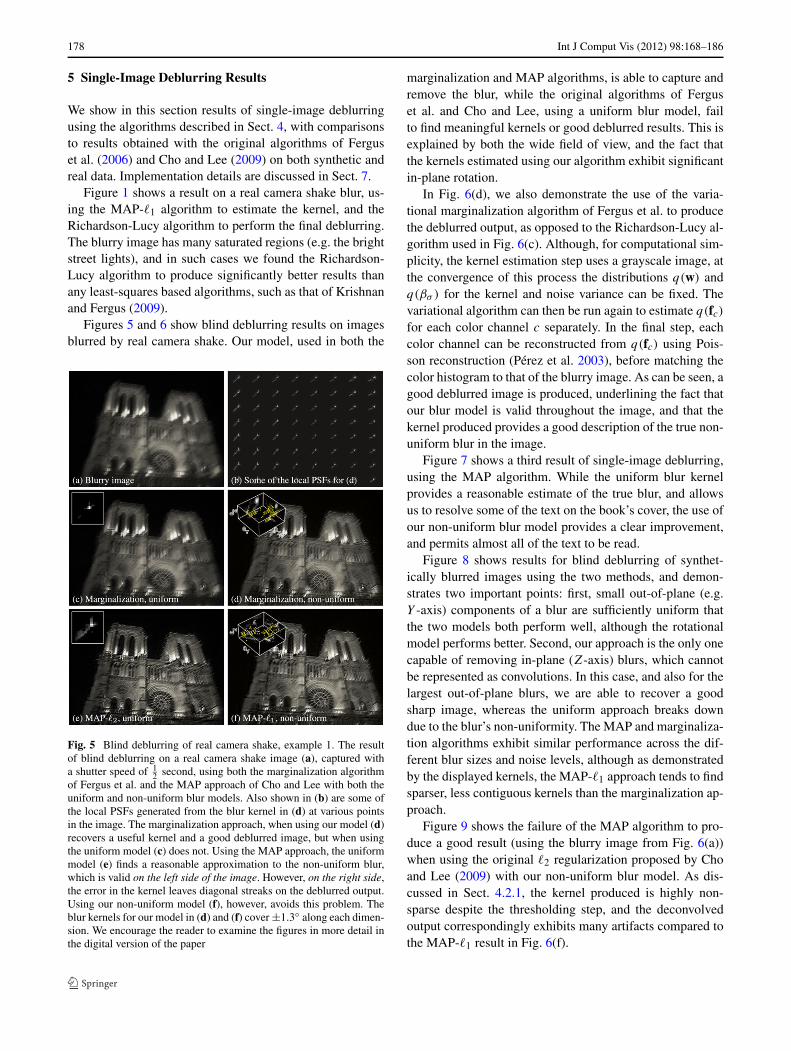
Figure 1 shows a result on a real camera shake blur, us-ing the MAP-�1 algorithm to estimate the kernel, and theRichardson-Lucy algorithm to perform the final deblurring.The blurry image has many saturated regions (e.g. the brightstreet lights), and in such cases we found the Richardson-Lucy algorithm to produce significantly better results thanany least-squares based algorithms, such as that of Krishnanand Fergus (2009).

Figures 5 and 6 show blind deblurring results on imagesblurred by real camera shake. Our model, used in both the

Fig. 5 Blind deblurring of real camera shake, example 1. The resultof blind deblurring on a real camera shake image (a), captured witha shutter speed of 1

2 second, using both the marginalization algorithmof Fergus et al. and the MAP approach of Cho and Lee with both theuniform and non-uniform blur models. Also shown in (b) are some ofthe local PSFs generated from the blur kernel in (d) at various pointsin the image. The marginalization approach, when using our model (d)recovers a useful kernel and a good deblurred image, but when usingthe uniform model (c) does not. Using the MAP approach, the uniformmodel (e) finds a reasonable approximation to the non-uniform blur,which is valid on the left side of the image. However, on the right side,the error in the kernel leaves diagonal streaks on the deblurred output.Using our non-uniform model (f), however, avoids this problem. Theblur kernels for our model in (d) and (f) cover ±1.3◦ along each dimen-sion. We encourage the reader to examine the figures in more detail inthe digital version of the paper

marginalization and MAP algorithms, is able to capture andremove the blur, while the original algorithms of Ferguset al. and Cho and Lee, using a uniform blur model, failto find meaningful kernels or good deblurred results. This isexplained by both the wide field of view, and the fact thatthe kernels estimated using our algorithm exhibit significantin-plane rotation.

In Fig. 6(d), we also demonstrate the use of the varia-tional marginalization algorithm of Fergus et al. to producethe deblurred output, as opposed to the Richardson-Lucy al-gorithm used in Fig. 6(c). Although, for computational sim-plicity, the kernel estimation step uses a grayscale image, atthe convergence of this process the distributions q(w) andq(βσ ) for the kernel and noise variance can be fixed. Thevariational algorithm can then be run again to estimate q(fc)for each color channel c separately. In the final step, eachcolor channel can be reconstructed from q(fc) using Pois-son reconstruction (Pérez et al. 2003), before matching thecolor histogram to that of the blurry image. As can be seen, agood deblurred image is produced, underlining the fact thatour blur model is valid throughout the image, and that thekernel produced provides a good description of the true non-uniform blur in the image.

Figure 7 shows a third result of single-image deblurring,using the MAP algorithm. While the uniform blur kernelprovides a reasonable estimate of the true blur, and allowsus to resolve some of the text on the book’s cover, the use ofour non-uniform blur model provides a clear improvement,and permits almost all of the text to be read.

Figure 8 shows results for blind deblurring of synthet-ically blurred images using the two methods, and demon-strates two important points: first, small out-of-plane (e.g.Y -axis) components of a blur are sufficiently uniform thatthe two models both perform well, although the rotationalmodel performs better. Second, our approach is the only onecapable of removing in-plane (Z-axis) blurs, which cannotbe represented as convolutions. In this case, and also for thelargest out-of-plane blurs, we are able to recover a goodsharp image, whereas the uniform approach breaks downdue to the blur’s non-uniformity. The MAP and marginaliza-tion algorithms exhibit similar performance across the dif-ferent blur sizes and noise levels, although as demonstratedby the displayed kernels, the MAP-�1 approach tends to findsparser, less contiguous kernels than the marginalization ap-proach.

Figure 9 shows the failure of the MAP algorithm to pro-duce a good result (using the blurry image from Fig. 6(a))when using the original �2 regularization proposed by Choand Lee (2009) with our non-uniform blur model. As dis-cussed in Sect. 4.2.1, the kernel produced is highly non-sparse despite the thresholding step, and the deconvolvedoutput correspondingly exhibits many artifacts compared tothe MAP-�1 result in Fig. 6(f).

Int J Comput Vis (2012) 98:168–186 179

Fig. 6 Blind deblurring of real camera shake, example 3. A hand-heldimage with camera shake (a), captured with a shutter speed of 1 second,with the results of blind deblurring using the marginalization algorithmof Fergus et al. under both a uniform (b) and non-uniform (c–d) blurmodel, and the MAP algorithm of Cho and Lee with a uniform (e) andnon-uniform (f) blur model. The variational output (d) is estimated us-ing the marginalization algorithm for the non-uniform case (calculated

as 〈f〉q(f) then converted from gradients to intensities using Poissonreconstruction—Pérez et al. 2003). The results using our blur modelshow more detail and fewer artifacts than those using the uniform blurmodel, as can be seen in the zoomed-in portions shown in the last row.The rotational blur kernels in (c) and (f) cover ±0.7◦ in θX and θY and±1.4◦ in θZ

In Fig. 10, we compare our approach to that of Ferguset al. (2006) on a real, uniformly blurred image, taken fromthe dataset of Levin et al. (2009), where the true blur isknown, and also known to be uniform. This demonstratesthe fact that our model includes uniform blur as a specialcase; by setting the focal length to be large and applying theconstraint that θZ = 0, we obtain results indistinguishablefrom those of Fergus et al. (2006). When we do not applythe constraint on θZ , our algorithm still produces a good re-sult, but unsurprisingly does not perform as well, since thenumber of kernel elements to be estimated is much larger(K is increased by a factor of 8).

Figure 11 shows the result of the non-uniform MAP-�1

approach on an image of Joshi et al. (2010). Although thescene is close to the camera, we are able to obtain a com-parable result to that of Joshi et al. without considering thecamera’s translational motion. This suggests that our deci-sion to ignore the camera’s translation is reasonable in prac-tice.

Besides comparing the results of a given algorithm witheither a uniform or non-uniform blur model, we can alsocompare the marginalization and MAP approaches for agiven model. In our experiments, we have observed that theMAP algorithm is generally more robust to the level of con-trast in the input image. The parameters of the image priorprovided by Fergus et al. (2006) are learnt from a single im-age of a street scene, so the application of this prior to animage with a very different distribution of pixels is liable toproduce poor results. The MAP algorithm however only re-lies on the ability to predict step edges from a blurry image,and adapts its threshold for predicting these edges depend-ing on the contrast of the image. On an image containingonly low-contrast edges then, such as in Fig. 1, the marginal-ization approach (using the street scene prior) fails to find auseful kernel, while the MAP approach finds a good kernel,as demonstrated by the comparison in Fig. 1(c). On the otherhand, as discussed by Cho and Lee (2009), the performanceof the MAP approach is sensitive to the values of the param-

180 Int J Comput Vis (2012) 98:168–186

Fig. 7 Blind deblurring of real camera shake, example 2. The resultof blind deblurring on a real camera shake image (a), captured witha shutter speed of 1 second, using the MAP approach of Cho and Leewith both the uniform and non-uniform blur models. Also shown in (b)are some of the local PSFs generated from the blur kernel in (d) atvarious points in the image. In the blurry image, most of the text onthe book cover is too blurred to read. Deblurring the image with theuniform blur model (c) allows some of the text on the cover of the bookto be read, however, after deblurring with our non-uniform model (d),all but the smallest text becomes legible. The blur kernel in (d) covers±0.4◦ in θX and θY , and ±0.9◦ in θZ

eters α and β , which must be manually specified, while themarginalization approach has almost no parameters to tune.

Convergence Neither of the algorithms can guarantee theability to arrive at a globally optimal solution. However, inpractice we have found them both to perform reliably. Byfinding a sequence of solutions at increasingly fine resolu-tions, the large scale structures in the blur kernel and sharpimage are resolved before the fine details. In the case of theMAP algorithm, each of the individual minimizations overthe sharp image f and the blur kernel w is convex, ensuring

convergence to a local minimum, even though the overallproblem is not jointly convex in both f and w. The gradi-ent prediction step helps direct the optimizations process to-wards a desirable minimum by encouraging the sharp imageto contain step edges. In the marginalization algorithm, wehave found that the algorithm converges equally reliably forboth the uniform model and our model in a similar numberof iterations.

Running Time An important difference between the twoapproaches is that the MAP algorithm typically takes a muchshorter amount of time to run, since the parameter updatesfor the marginalization algorithm, given in (23)–(26), arecomputationally expensive. Due to this expense, and thelarger number of iterations required for our model comparedto the uniform model, the marginalization algorithm withour non-uniform model can take several hours to deblur animage of several hundred pixels across on a modern work-station. Deblurring larger images with this method is notcurrently practical, whereas the MAP algorithm can deblurthe same images in under an hour.

Limitations Both of these algorithms are capable of re-moving large blurs—up to around 50 pixels across, for bothuniform and non-uniform blur. For our model, this corre-sponds to around 3◦–5◦ of rotation around each axis for aphotograph whose width and focal length are both 1000 px.Since we have assumed that camera translation has a negli-gible blurring effect, our model (and in general the uniformmodel too) is unlikely to produce good results on imagesfor which this is not true, due to the depth-dependent blurproduced. Another typical failure case for the MAP algo-rithm comes from the fact that it relies on the ability to pre-dict sharp step edges from blurry ones, which may not bethe case on images which contain only fine-scale texture, orwhere the blur is too large to allow this.

6 Deblurring with Noisy/Blurry Image Pairs

In this section, we apply our model to the case where, inaddition to g, we have a sharp but noisy image fN of thesame scene, as proposed by Yuan et al. (2007a). The mo-tivation for this is that in low light, blurry images occur atlong shutter speeds, however it is often also possible to usea short exposure at a high ISO setting to obtain a sharp butnoisy image of the same scene. While the noisy image maybe degraded too badly to allow the direct recovery of a goodsharp image, it can initially be used as a proxy for the sharpimage, allowing us to estimate the blur kernel w by solv-ing (15). Following this, the kernel is assumed to be known,and used to deblur g, solving (14). The noisy image can alsobe used to improve this deconvolution step, and Yuan et al.

Int J Comput Vis (2012) 98:168–186 181

Fig. 8 Blind deblurring of synthetic single-axis blurs. A sharp image(top left) with examples of synthetic blur by rotation of the cameraabout its Y - and Z-axis, and the kernels and deblurred results for dif-ferent cases. We compare the results of blind deblurring for two sizesof blur and three noise levels, and the reconstruction errors are summa-rized in the table at the top. For each single-axis blur, the table containsthe root-mean-square (RMS) errors between the deblurred results and

the ground-truth sharp image for blurs with a maximum size of 10 or20 pixels in the image, using our non-uniform model and the uniformmodel. In each cell we also show, in parentheses, the ratio between theRMS error and the corresponding error for that blurry image deblurredwith the ground-truth kernel. Note that to facilitate comparison withoutthe influence of image priors, the deblurred images were all producedusing the Richardson-Lucy algorithm

Fig. 9 Poor performance of MAP-�2 with non-uniform blur model.The corresponding blurry image can be seen in Fig. 6. Shown is the es-timated kernel and deblurred result when using our non-uniform blurmodel in the algorithm of Cho and Lee with �2 regularization on thekernel. As can be seen, the �2 regularization is not sufficient to pro-duce a good estimate of the kernel, and results in a deblurred outputcontaining many artifacts

propose a modified version of the Richardson-Lucy algo-rithm, which uses fN to suppress artifacts in the result.

6.1 Kernel Estimation

As discussed in Sect. 3.2, some prior knowledge must be ap-plied to recover a good kernel estimate. In their algorithm,Yuan et al. (2007a) constrain the kernel to have non-negativeelements and unit �1 norm, however they simultaneouslypenalize the �2 norm of the kernel, reducing the sparsity-inducing effect of the constraint. To help find a sparse kernel,they propose a thresholding scheme which sets some kernelelements to zero at each iteration. In our approach, we optto use the �1 and positivity constraints alone, since they leadnaturally to a sparse kernel (Tibshirani 1996), a fact also ex-ploited by Shan et al. (2007) for blur kernel estimation.

In order to estimate the blur kernel, we minimize the fol-lowing energy function:

182 Int J Comput Vis (2012) 98:168–186

Fig. 10 Blind deblurring of a real uniform blur. A real camera shakeblur (a–b) from the dataset of Levin et al. (2009), deblurred using ker-nels estimated with the marginalization algorithm. We show deblurredresults and kernels for four cases; (c) uniform blur using original algo-rithm of Fergus et al., (d) our model with a large focal length F and noin-plane rotation (θZ = 0), (e) our approach with a large focal length F

but with θZ unconstrained, and (f) the ground-truth (uniform) kernel,provided with the dataset. Note that (d) is indistinguishable from (c),apart from a translation, and that the kernel in (d), while not perfect,does have the same diagonal shape as the true blur, with the non-zeroscentered around a single value of θZ

Fig. 11 Blind deblurring of an image from Joshi et al. (2010). A hand-held image with camera shake (a), from Joshi et al. (2010), with thedeblurred results from the original work (b) and using the MAP-�1method with our blur model (c). We obtain a comparable result, with-

out the use of additional hardware and without considering the cam-era’s translation during the exposure, despite the scene being close tothe camera

EN(w) = ‖g(fN,w) − g‖22

s.t. ∀ k = 1, . . . ,K, wk ≥ 0 and∑

k

wk = 1, (34)

where, by analogy with (15), g(fN,w) = BNw, and BN isthe matrix whose columns each contain a projectively trans-formed copy of fN . Similar to (29), this least-squares for-mulation with non-negative �1 constraints can be solved ef-ficiently (Kim et al. 2007; Mairal et al. 2010). Since the en-ergy function is convex with convex constraints, we can besure of reaching the global minimum.

For comparison, we have also implemented this algo-rithm for uniform blurs, using a matrix BN in (34) whose

columns contained translated versions of fN , rather than pro-jectively transformed versions.

6.2 Image Reconstruction

Having estimated the blur kernel, Yuan et al. (2007a) pro-pose several modifications to the Richardson-Lucy (RL) al-gorithm, which take advantage of the fact that it is possibleto recover much of the low-frequency content of f from a de-noised version of fN . Images deblurred with the standard RLalgorithm often exhibit “ringing” artifacts—low-frequencyripples spreading across the image, such as in Fig. 9—butusing the denoised image it is possible to disambiguate thetrue low frequencies from these artifacts, and largely remove

Int J Comput Vis (2012) 98:168–186 183

them from the result. Doing this significantly improves thedeblurred results compared to the standard RL algorithm.We refer the reader to Yuan et al. (2007a) for full details ofthe augmented RL algorithm, omitted here for brevity. Wehave adapted the algorithm for our non-uniform blur model,along the same lines as for the standard RL algorithm inSect. 4.3.

6.3 Results

In this section, we present results with noisy/blurry imagepairs, and refer the reader to Sect. 7 for implementation de-tails. Figures 12 and 13 show a comparison between the uni-form model and ours, using the algorithm described aboveto estimate the blur kernels. Having estimated the kernel,we deblur the blurred images using the augmented RL al-gorithm of Yuan et al. (2007a). As can be seen from thedeblurred images obtained with the two models, our resultsexhibit more detail and fewer artifacts than those using theuniform blur model.

7 Implementation

The implementation of the variational kernel estimationmethod presented in Sect. 4.1 is based on the code madeavailable by Miskin and MacKay (2000) and by Fergus et al.(2006).2 We have modified the algorithm to use our blurmodel and replaced the parameter update equations with thecorresponding versions derived for our bilinear blur modelin (23)–(26). A package containing our code is available on-line.3 The implementation of the image reconstruction algo-rithm of Krishnan and Fergus (2009) is also based on MAT-LAB code made available online by the authors.4 The imple-mentations of the Richardson-Lucy algorithm, the algorithmof Cho and Lee (2009), and the augmented RL algorithm ofYuan et al. (2007a) are our own, and we use these imple-mentations for both uniform and non-uniform blur modelswhen comparing results. A binary executable for Cho andLee’s algorithm is available, however we did not observe animprovement in the results obtained, and thus use our ownimplementation to permit a fairer comparison between theresults from the uniform and non-uniform blur models.

7.1 Sampling the Set of Rotations

One important detail to consider is how finely to discretizethe orientation parameter θ . Undersampling the set of ori-entations will affect our ability to accurately reconstruct the

2http://cs.nyu.edu/~fergus/research/deblur.html.3http://www.di.ens.fr/willow/research/deblurring/.4http://cs.nyu.edu/~dilip/research/fast-deconvolution/.

Fig. 12 Deblurring real camera shake blur using a noisy/blurry im-age pair. A noisy image (a) and a blurry image (b) captured with ahand-held camera, with the estimated kernels (c–d) and deblurred re-sults (f–g) for the uniform and non-uniform blur models. Also shownfor illustration are a selection of the local PSFs generated by the rota-tional kernel (e). As can be seen in the close-ups (h–k), our result (k)contains more details and fewer artifacts than when using the uniformblur model (j), and reveals features not visible in either the noisy or theblurry image. The non-uniform kernel in (d) covers ±3◦ along each di-mension. We encourage the reader to examine the images in the digitalversion of the paper

184 Int J Comput Vis (2012) 98:168–186

Fig. 13 Deblurring real camera shake blur using a noisy/blurry imagepair. A noisy image (a) and blurry image (b) captured with a hand-heldcamera, shown with the estimated kernels (c–d) and deblurred im-ages (e–f) for the uniform and non-uniform blur models. Note in theclose-up that the result using our model (j) has sharper edges and fewerartifacts than that using the uniform model (i). The non-uniform kernelin (d) covers ±3◦ along each dimension

blurred image, but sampling it too finely will lead to unnec-essary calculations. Since the kernel is defined over the 3parameters θX , θY and θZ , doubling the sampling resolutionincreases the number of kernel elements by a factor of 8.In practice, we have found that a good choice of grid spac-ing is that which corresponds to a maximum displacementof 1 pixel in the image. Since we are fundamentally lim-ited by the resolution of our images, reducing the spacingfurther leads to redundant orientations, which are indistin-guishable from their neighbors. Setting the grid spacing interms of pixels also has the advantage that our 3D blur ker-nels are defined on a grid which allows direct comparisonto the pixel grid of the image. We set the size of our ker-nel along each dimension in terms of the size of the blur weneed to model, typically a few degrees along each dimensionof θ , e.g. [−5◦,5◦].

7.2 Multiscale Implementation

All of the kernel estimation algorithms presented here areapplied within a multiscale framework, starting with acoarse representation of image and kernel, and repeatedly

refining the estimated kernel at higher resolutions. In thecase of single-image deblurring, this is essential to avoidpoor local minima, however it is also important for compu-tational reasons in both the single-image and noisy/blurryimage pair cases. The kernel at the original image resolutionmay have thousands or tens of thousands of elements, how-ever very few of these should have non-zero values. For ex-ample to solve (34) directly at full resolution would involvetransforming fN for every possible rotation under consider-ation and storing all the copies simultaneously in BN . Thisrepresents a significant amount of redundant computation,since most of these copies will correspond to zeros in thekernel, and furthermore BN may have too many columns tofit in the computer’s memory. The effect on the computa-tion and memory requirements for single-image deblurringis comparable.

Thus, in all of the applications presented in this paper,we use the solution ws at each scale s to constrain the so-lution at the next scale ws+1, by defining an “active region”where ws is non-zero, and constraining the non-zeros at thenext scale to lie within this region. In the example above,this corresponds to discarding many columns of BN , reduc-ing both the computation and memory demands of the al-gorithm. We first build Gaussian pyramids for the blurredimage (and noisy image, if applicable), and at the coarsestscale s = 0, define the active region to cover the full kernel.At each scale s, we find the optimal kernel ws for that scale.We then upsample ws to the next scale (s + 1) using bilinearinterpolation, find the non-zero elements of this upsampledkernel, and dilate this region using a 3 × 3 × 3 cube. Whenfinding the optimal kernel ws+1, we fix all elements out-side the active region to zero. We repeat this process at eachscale, until we have found the optimal kernel at the finestscale.

7.3 Geometric and Photometric Registration

For the case of noisy/blurry image pairs, the two images aresimply taken one after the other with a hand-held camera,so they may not be registered with each other. Thus, we es-timate an approximate registration θ0 between them at thecoarsest scale, using an exhaustive search over a large setof rotations, for example ±10◦ about all 3 axes using thesame step size as for the blur kernel, and we remove thismis-registration from the noisy image. When applying theuniform blur model in this case, we manually estimate thein-plane rotation to best register the two images, as in Yuanet al. (2007a).

To compensate for the difference in exposure between thenoisy and blurry images, at each scale s, after computing ws

for that scale, we estimate a linear rescaling a by computingthe linear least-squares fit between the pixels of gs and thoseof gs(ws , fN,s), and apply this to the noisy image, i.e. fN ←afN .

Int J Comput Vis (2012) 98:168–186 185

8 Conclusion

We have proposed a new model for camera shake, derivedfrom the geometric properties of cameras, and applied itto two deblurring problems within the frameworks of ex-isting camera shake removal algorithms. We have validatedthe model with experiments on real and synthetic data,demonstrating superior results compared to the uniform blurmodel. The model assumes that the motion of the cameraduring exposure is limited to rotations about its optical cen-ter, and is temporally-agnostic to the distribution over cam-era orientations. Note, however, that camera rotations thatare off the optical center can be modeled by camera rota-tions about the optical center together with translation; thesetranslations should generally be small for rotation centersthat are not far from the optical center. The model is not ap-plicable for non-static scenes, or nearby scenes with largecamera translations where parallax effects may become sig-nificant.

In the future, we plan to investigate the use of our generalbilinear model to other non-uniform blurs. We also plan toinvestigate means of reducing the computational overheadof the model, for example with the use of a suitable approx-imation strategy, such as Hirsch et al. (2010).

Acknowledgements We are grateful for discussions with BryanRussell, and comments from Fredo Durand and the reviewers. Thankyou to James Miskin and Rob Fergus for making their code available.Financial support was provided by ONR MURI N00014-07-1-0182,ERC grant VisRec no. 228180, the MSR-INRIA laboratory, ANRgrant HFIBMR (ANR-07-BLAN-0331-01), the EIT-ICT labs (activity10863), and the ERC grant VideoWorld.

Appendix A: Parameter Update Equations forMarginalization Algorithm

Equations (23)–(26) cannot be evaluated directly, since theyinvolve expectations over combinations of variables. For im-plementation they must be expanded and written in terms ofthe mean and variance of individual variables. Here we givethese expansions, which are exactly the parameter updatescomputed in our implementation. First, let

vwk = 〈w2

k〉 − 〈wk〉2, (35)

vfj = 〈f 2

j 〉 − 〈fj 〉2, (36)

〈Aij 〉 =∑

k

Cijk〈wk〉, (37)

〈Bik〉 =∑j

Cijk〈fj 〉, (38)

〈gi〉 =∑

k

(∑j

Cijk〈fj 〉)

〈wk〉. (39)

Then,

w(2)k = 〈βσ 〉

∑i,j

C2ijkv

fj + 〈βσ 〉

∑i

〈Bik〉2, (40)

w(1)k w

(2)k = 〈βσ 〉

∑i

〈Bik〉(gi − 〈gi〉)

− 〈βσ 〉∑i,j

Cijk〈Aij 〉vfj + 〈wk〉w(2)

k , (41)

f(2)j = 〈βσ 〉

∑i,k

C2ijkv

wk + 〈βσ 〉

∑i

〈Aij 〉2, (42)

f(1)j f

(2)j = 〈βσ 〉

∑i

〈Aij 〉(gi − 〈gi〉)

− 〈βσ 〉∑i,k

Cijk〈Bik〉vwk + 〈fj 〉f (2)

j . (43)

Finally, in evaluating the parameters of the distributionq(βσ ) for the variance of the noise (Miskin and MacKay2000, (40)), it is necessary to evaluate the following quan-tity:

〈(gi − gi )2〉 = (gi − 〈gi〉)2 +

∑j,k

C2ijkv

fj vw

k

+∑j

〈Aij 〉2vfj +

∑k

〈Bik〉2vwk . (44)

Appendix B: Computation of Interpolation Coefficients

Here we give details of how the values of Cijk can be cal-culated if bilinear interpolation is used. Note that these arestandard interpolation weights, and are not specific to thisdeblurring application. We consider a pixel gi in the blurryimage which is mapped under a homography Hk to a pointx′ in the sharp image, i.e. Hkxi ∼ (x′, y′,1)�. The point x′will, in general, be a sub-pixel location, and the value ofthe sharp image f at x′ is interpolated from the 4 pixels sur-rounding x′, using the following weights:

(xj , yj ) Cijk

(�x′�, �y′� )

(�x′�, �y′� + 1)

(�x′� + 1,�y′� )

(�x′� + 1,�y′� + 1)

(�x′� + 1− x′ )(�y′� + 1− y′ )

(�x′� + 1− x′ )( y′ −�y′�)( x′ −�x′�)(�y′� + 1− y′ )

( x′ −�x′�)( y′ −�y′�)

where � · � takes the integer part of a positive scalar. The cor-respondence between a pixel fj ’s index j and coordinates(xj , yj ) can be obtained using, for example, the MATLAB

functions ind2sub / sub2ind.

186 Int J Comput Vis (2012) 98:168–186

References

Banham, M. R., & Katsaggelos, A. K. (1997). Digital image restora-tion. IEEE Signal Processing Magazine, 14(2), 24–41.

Bishop, C. M. (2006). Pattern recognition and machine learning(information science and statistics). Berlin: Springer. ISBN0387310738.

Cai, J.-F., Ji, H., Liu, C., & Shen, Z. (2009). Blind motion deblurringfrom a single image using sparse approximation. In Proc. CVPR.

Chakrabarti, A., Zickler, T., & Freeman, W. T. (2010). Analyzingspatially-varying blur. In Proc. CVPR.

Chan, T. F., & Wong, C.-K. (1998). Total variation blind deconvolution.IEEE Transactions on Image Processing, 7(3).

Chen, J., Yuan, L., Tang, C.-K., & Quan, L. (2008). Robust dual motiondeblurring. In Proc. CVPR.

Cho, S., & Lee, S. (2009). Fast motion deblurring. ACM Transactionson Graphics, 28(5), 145:1–145:8 (Proc. SIGGRAPH Asia 2009).

Cho, S., Matsushita, Y., & Lee, S. (2007). Removing non-uniform mo-tion blur from images. In Proc. ICCV.

Couzinie-Devy, F., Mairal, J., Bach, F., & Ponce, J. (2011). Dictionarylearning for deblurring and digital zoom (submitted). PreprintHAL: inria-00627402.

Dabov, K., Foi, A., Katkovnik, V., & Egiazarian, K. (2008). Imagerestoration by sparse 3D transform-domain collaborative filtering.In SPIE electronic imaging.

Efron, B., Hastie, T., Johnstone, L., & Tibshirani, R. (2004). Least an-gle regression. Annals of Statistics, 32(2), 407–499.

Fergus, R., Singh, B., Hertzmann, A., Roweis, S. T., & Freeman, W. T.(2006). Removing camera shake from a single photograph. ACMTransactions on Graphics, 25(3), 787–794 (Proc. SIGGRAPH2006).

Gupta, A., Joshi, N., Zitnick, C. L., Cohen, M., & Curless, B. (2010).Single image deblurring using motion density functions. In Proc.ECCV.

Hartley, R. I., & Zisserman, A. (2004). Multiple view geometry in com-puter vision (2nd edn.). Cambridge: CUP. ISBN 0521540518.

Hirsch, M., Sra, S., Schölkopf, B., & Harmeling, S. (2010). Efficientfilter flow for space-variant multiframe blind deconvolution. InProc. CVPR.

Joshi, N., Kang, S. B., Zitnick, C. L., & Szeliski, R. (2010). Imagedeblurring using inertial measurement sensors. ACM Transactionson Graphics, 29(4), 30:1–30:9 (Proc. SIGGRAPH 2010).

Kim, S.-J., Koh, K., Lustig, M., Boyd, S., & Gorinevsky, D. (2007). Aninterior-point method for large-scale �1-regularized least squares.IEEE Journal of Selected Topics in Signal Processing, 1(4), 606–617.

Klein, G., & Drummond, T. (2005). A single-frame visual gyroscope.In Proc. BMVC.

Krishnan, D., & Fergus, R. (2009). Fast image deconvolution usinghyper-Laplacian priors. In NIPS.

Lee, D. D., & Seung, H. S. (2001). Algorithms for non-negative matrixfactorization. In NIPS.

Levin, A. (2006). Blind motion deblurring using image statistics. InNIPS.

Levin, A., Weiss, Y., Durand, F., & Freeman, W. T. (2009). Under-standing and evaluating blind deconvolution algorithms. In Proc.CVPR.

Lim, S. H., & Silverstein, A. (2008). Estimation and removal of motionblur by capturing two images with different exposures. TechnicalReport HPL-2008-170, HP Laboratories.

Lucy, L. B. (1974). An iterative technique for the rectification of ob-served distributions. Astronomical Journal, 79(6), 745–754.

Mairal, J., Bach, F., Ponce, J., & Sapiro, G. (2010). Online learningfor matrix factorization and sparse coding. Journal of MachineLearning Research, 11, 19–60.

Miskin, J. W., & MacKay, D. J. C. (2000). Ensemble learning for blindimage separation and deconvolution. In M. Girolani (Ed.), Ad-vances in independent component analysis. Berlin: Springer.

Nagy, J. G., & O’Leary, D. P. (1998). Restoring images degradedby spatially variant blur. SIAM Journal on Scientific Computing,19(4), 1063–1082.

Osher, S., & Rudin, L. I. (1990). Feature oriented image enhancementusing shock filters. SIAM Journal on Numerical Analysis, 27(4),919–940.

Pérez, P., Gangnet, M., & Blake, A. (2003). Poisson image edit-ing. ACM Transactions on Graphics, 22(3), 313–318 (Proc. SIG-GRAPH 2003).

Puetter, R. C., Gosnell, T. R., & Yahil, A. (2005). Digital image recon-struction: deblurring and denoising. Annual Review of Astronomyand Astrophysics, 43, 139–194.

Rav-Acha, A., & Peleg, S. (2005). Two motion-blurred images are bet-ter than one. Pattern Recognition Letters, 26(3).

Richardson, W. H. (1972). Bayesian-based iterative method of imagerestoration. Journal of the Optical Society of America, 62(1), 55–59.

Sawchuk, A. A. (1974). Space-variant image restoration by coordinatetransformations. Journal of the Optical Society of America, 64(2),138–144.

Shan, Q., Xiong, W., & Jia, J. (2007). Rotational motion deblurring ofa rigid object from a single image. In Proc. ICCV.

Shan, Q., Jia, J., & Agarwala, A. (2008). High-quality motion deblur-ring from a single image. ACM Transactions on Graphics, 27(3)(Proc. SIGGRAPH 2008).

Tai, Y.-W., Tan, P., Gao, L., & Brown, M. S. (2009). Richardson-Lucydeblurring for scenes under projective motion path. Technical re-port, KAIST.

Tai, Y.-W., Du, H., Brown, M. S., & Lin, S. (2010a). Correction of spa-tially varying image and video motion blur using a hybrid camera.IEEE Transactions on Pattern Analysis and Machine Intelligence,32(6), 1012–1028.

Tai, Y.-W., Kong, N., Lin, S., & Shin, S. Y. (2010b). Coded exposureimaging for projective motion deblurring. In Proc. CVPR.

Tai, Y.-W., Tan, P., & Brown, M. S. (2011). Richardson-Lucy deblur-ring for scenes under a projective motion path. IEEE Transactionson Pattern Analysis and Machine Intelligence, 33(8), 1603–1618.

Tibshirani, R. (1996). Regression shrinkage and selection via the lasso.Joutnal of the Royal Statistical Society, Series B, 58(1), 267–288.

Tomasi, C., & Manduchi, R. (1998). Bilateral filtering for gray andcolor images. In Proc. ICCV.

Vio, R., Nagy, J., Tenorio, L., & Wamsteker, W. (2005). Multiple imagedeblurring with spatially variant PSFs. Astronomy & Astrophysics,434, 795–800.

Xu, L., & Jia, J. (2010). Two-phase kernel estimation for robust motiondeblurring. In Proc. ECCV.

Yuan, L., Sun, J., Quan, L., & Shum, H.-Y. (2007a). Image deblurringwith blurred/noisy image pairs. ACM Transactions on Graphics,26(3) (Proc. SIGGRAPH 2007).

Yuan, L., Sun, J., Quan, L., & Shum, H.-Y. (2007b). Blurred/non-blurred image alignment using sparseness prior. In Proc. ICCV.

Yuan, L., Sun, J., Quan, L., & Shum, H.-Y. (2008). Progressive inter-scale and intra-scale non-blind image deconvolution. ACM Trans-actions on Graphics, 27(3) (Proc. SIGGRAPH 2008)