Non-Parametric Estimation of

Second Order Stochastic Di¤erential Equations

João Nicolau

Instituto Superior de Economia e Gestão

Universidade Técnica de Lisboa

October, 2006

Abstract

We propose non-parametric estimators of the in�nitesimal coe¢ cients associated with second order sto-chastic di¤erential equations. We show that under appropriate conditions, the proposed estimators areconsistent. Also, we state conditions ensuring the asymptotic normality of these estimators. We concludeour paper with a Monte Carlo experiment in which we assess the response of the nonparametric estimatorswith respect to the step of discretization.

1 Introduction

In economics and �nance many stochastic processes can be seen as integrated stochastic processes

in the sense that the current observation behaves as the cumulation of all past perturbations. In a

discrete-time framework the concept of integration and di¤erentiation of a stochastic process

plays an essential role in modern econometric analysis. For instance, the stochastic process

fyt; t = 0; 1; 2; :::g where yt = � + yt�1 + "t ("t � i:i:d:N (0; 1)) is an example of an integrated

process. Notice that y can be written as yt = y0 + t�+Pt

k=1 "k, or

yt = y0 +

tXk=1

xk; (1)

where xt = � + "t: One way to deal with such processes is to use a di¤erenced-data model (for

example, �yt = �+ "t; in the previous example). Di¤erencing has been used mostly to solve non-

stationary problems viewed as unit roots although, historically, di¤erenced-data models arose early

in econometrics as a procedure to remove common trends between dependent and independent

variables.

Integrated and di¤erentiated di¤usion processes in the same sense as integrated and di¤er-

entiated discrete-time processes are almost absent in applied econometrics analysis. One of the

reasons continuous-time di¤erentiated processes have not been considered in applied econometrics

is, perhaps, related to the di¢ culties in interpreting the �di¤erentiated�process. In fact, if Z is

a di¤usion process driven by a Brownian motion, then all sample functions are of unbounded

variation and nowhere di¤erentiable, i.e. dZt=dt does not exist with probability one (unless some

smoothing e¤ect of the measurement instrument is introduced, such as described in Arnold, 1974).

One way to model integrated and di¤erentiated di¤usion processes and overcome the di¢ culties

associated with the nondi¤erentiability of the Brownian motion is through the representation8>><>>:dYt = Xtdt

dXt = a (Xt) dt+ b (Xt) dWt

(2)

where a and b are the in�nitesimal coe¢ cients (respectively, the drift and the di¤usion coe¢ cient),

1

W is a (standard) Wiener process (or Brownian motion) and X is (by hypothesis) a stationary

process. In this model, Y is a di¤erentiable process, by construction. It represents the integrated

process,

Yt = Y0 +

Z t

0

Xudu (3)

(note the analogy with the corresponding expression in a discrete-time setting, yt = y0+Pt

k=1 xk;

equation (1)) and Xt = dYt=dt is the stationary di¤erentiated process (which can be considered

the equivalent concept to the �rst di¤erences sequence in discrete-time analysis). If X represents

the continuously compounded return or log return of an asset, the �rst equation in system (2)

should be rewritten as d log Yt = Xtdt:

We think that (2) can be a useful model in empirical �nance for at least two reasons. First,

the model accommodates nonstationary integrated stochastic processes (Y ) that can be made

stationary by di¤erencing. Such transformation cannot be undertaken in common univariate

di¤usion processes used in �nance (because all sample paths from univariate di¤usion processes

are nowhere di¤erentiable with probability one). Yet, many processes in economics and �nance

(e.g. stock prices and nominal exchange rates) behave as the cumulation of all past perturbations

(basically in the same sense as unit root processes in discrete framework). Second, in the context of

stock prices or exchange rates, the model suggests directly modelling the (instantaneous) returns,

in contrast to usual continuous-time models in �nance, which directly model the prices. General

properties for returns (stylized facts) are well known and documented (for example, returns are

generally stationary in mean, the distribution is not normal, the autocorrelations are weak and

the correlations between the magnitude of returns are positive and statistically signi�cant, etc.).

One advantage of directly modelling the returns (X) is that these general properties are easier to

specify in a model like (2) than in a di¤usion univariate process for the prices. In fact, several

interesting models can be obtained by selecting a (x) and b2 (x) appropriately. For example, the

choice a (x) = � (� � x) and b (x) =q�2 + � (Xt � �)2 leads to an integrated process Y whose

returns, X; have an asymmetric leptokurtic stationary distribution (see the example below). This

2

speci�cation can be appropriated in �nancial time series data. Bibby and Sørensen (1997) had

already noticed that a similar process to (2) could be a good model for stock prices.

We observe that the model de�ned in equation (2) can be written as a second order stochastic

di¤erential equation, d (dYt=dt) = a (Xt) dt+ b (Xt) dWt: Integrated di¤usions like Y in equation

(3) arise naturally when only observations of a running integral of the process are available.

For instance, this can occur when a realization of the process is observed after passage through

an electronic �lter. Another example is provided by ice-core data on oxygen isotopes used to

investigate paleo-temperatures (see Ditlevsen and Sørensen, 2004).

To illustrate continuous-time integrated processes, �gure 1 presents two simulated independent

paths of Yt = Y0 +R t0Xudu where X is governed by the stochastic di¤erential equation

dXt = 20 (0:01�Xt) dt+q0:1 + 10 (Xt � 0:05)2dWt

(X is also represented in �gure 1). All paths are composed of 1000 observations de�ned in the

interval t 2 [0; 10] : In section 4 we give more details on how we generate these observations. It is

interesting to observe that Y displays all the features of an integrated process (with a positive drift,

since E [Xt] = 0:01): absence of mean reversion, shocks are persistent, mean and variance depend

on time, etc. On the other hand, the unconditional distribution of X (return) is asymmetric and

leptokurtic.

** FIGURE 1 HERE**

Estimation of second order stochastic di¤erential equations raises new challenges for two main

reasons. On the one hand, only the integrated process Y is observable at instants fti; i = 1; 2; :::g

and thus X in model (2) is a latent non-observable process. In fact, for a �xed sampling interval,

it is impossible to obtain the value of X at time ti from the observation Yti which represents the

3

integral Y0+R ti0Xudu. On the other hand, the estimation of model (2) cannot in principle be based

on the observations fYti ; i = 1; 2; :::g since the conditional distribution of Y is generally unknown,

even if that of X is known. An exception is the case where X follows an Orstein-Uhlenbeck

process, which is analyzed in Gloter (2001).

However, with discrete-time observations fYi�; i = 1; 2; :::g (to simplify we use the notation

ti = i�; where � = ti � ti�1), and given that

Yi� � Y(i�1)� =Z i�

0

Xudu�Z (i�1)�

0

Xudu =

Z i�

(i�1)�Xudu;

we can obtain a measure of X at instant ti = i� using the formula:

~Xi� =Yi� � Y(i�1)�

�: (4)

Naturally, the accuracy of (4) as a proxy for Xi� depends on the magnitude of �: Regardless

of the magnitude of � we have in our sample, we should base our estimation procedures on the

samplen~Xi�

o:=n~Xi�; i = 0; 1; 2; :::

osince X is not observable.

Parametric and semi-parametric estimation of integrated di¤usions is analyzed in Gloter (1999,

2006) and Ditlevsen and Sørensen (2004).

We suppose that both in�nitesimal coe¢ cients a and b; de�ned in model (2), are unknown and

our aim is their non-parametric functional estimation. We propose non-parametric estimators for

the in�nitesimal coe¢ cients a and b: Our analysis reveals that the standard estimators based on

the samplen~Xi�

oare inconsistent, even if we allow the step of discretization � to go to zero

asymptotically. Introducing slight modi�cations to these estimators we provide consistent estima-

tors. For a review on non-parametric estimation of (�rst order) stochastic di¤erential equations

see, for example, Rao (1983), Florens-Zmirou (1993), Jiang and Knight (1997), Bandi and Phillips

(2003), Nicolau (2003) and Gobet et al. (2004). For a review on parametric and semi-parametric

estimation see, for example, Aït-Sahalia (2002) and Kessler (1997) and the references therein.

The rest of the paper is organized as follows. In section 2 we formulate the main hypotheses

concerning the X process and we identify our estimators. In section 3 we establish the main

4

results. We show that under appropriate conditions, the proposed estimators are consistent and

asymptotically normal. In section 4 we perform a Monte Carlo experiment in which we assess the

response of the nonparametric estimator with respect to the step of discretization �: Section 5

concludes.

2 Estimators and Assumptions

The aim of this paper is to study the following estimators,

pn (x) =1

nhn

nXi=1

K

x� ~X(i�1)�n

hn

!; an (x) =

An (x)

pn (x); b2n (x) =

Bn (x)

pn (x)(5)

for, respectively, p (x) ; a (x) and b2 (x) ; based on the observationsn~Xi�n

o; where

An (x) =1

nhn

nXi=1

K

x� ~X(i�1)�n

hn

! � ~X(i+1)�n� ~Xi�n

��n

; (6)

Bn (x) =1

nhn

nXi=1

K

x� ~X(i�1)�n

hn

! 32

�~Xi�n � ~X(i�1)�n

�2�n

: (7)

Consider the process (Y;X) governed by the system (2). Let I = (l; r) the state space of X: Let

s (z) = expn�R zz02a (u) =b2 (u) du

obe the scale density function (z0 is an arbitrary point inside

I) and m (u) =�b2 (u) s (u)

��1the speed density function. Let S (l; x] = limx1!l

R xx1s (u) du and

S [x; r) = limx2!r

R x2xs (u) du where, l < x1 < x < x2 < r. We now present a set of eight

assumptions that are used throughout the paper.

A1 S (l; x] = S [x; r) =1 for x 2 I.

A2R rlm (x) dx <1.

A1 and A2 conditions assure that X is ergodic and the invariant distribution P 0 has density

p (x) = m (x) =R rlm (u) du with respect to the Lebesgue measure (Skorokhod, 1989, theorem 16).

The expression p (x) is usually referred to as the stationary density.

A3 X0 = x has distribution P 0.

5

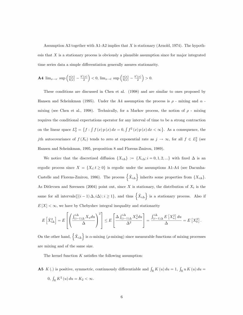
Assumption A3 together with A1-A2 implies that X is stationary (Arnold, 1974). The hypoth-

esis that X is a stationary process is obviously a plausible assumption since for major integrated

time series data a simple di¤erentiation generally assures stationarity.

A4 limx!r sup�a(x)b(x) �

b0(x)2

�< 0, limx!l sup

�a(x)b(x) �

b0(x)2

�> 0:

These conditions are discussed in Chen et al. (1998) and are similar to ones proposed by

Hansen and Scheinkman (1995). Under the A4 assumption the process is � - mixing and � -

mixing (see Chen et al., 1998). Technically, for a Markov process, the notion of � - mixing

requires the conditional expectations operator for any interval of time to be a strong contraction

on the linear space L02 =�f :Rf (x) p (x) dx = 0;

Rf2 (x) p (x) dx <1

. As a consequence, the

jth autocovariance of f (Xt) tends to zero at exponential rate as j ! 1, for all f 2 L02 (see

Hansen and Scheinkman, 1995, proposition 8 and Florens-Zmirou, 1989).

We notice that the discretized di¤usion fXi�g := fXi�; i = 0; 1; 2; :::g with �xed � is an

ergodic process since X = fXt; t � 0g is ergodic under the assumptions A1-A4 (see Dacunha-

Castelle and Florens-Zmirou, 1986). The processn~Xi�

oinherits some properties from fXi�g.

As Ditlevsen and Sørensen (2004) point out, since X is stationary, the distribution of Xt is the

same for all intervalsf[(i� 1)�; i�) ; i � 1g, and thusn~Xi�

ois a stationary process. Also if

E [X] <1, we have by Chebyshev integral inequality and stationarity

Eh~X2i�

i= E

2640@R i�(i�1)�Xudu

�

1A2375 � E

24� R i�(i�1)�X2udu

�2

35 = R i�(i�1)�E �X2u

�du

�= E

�X20

�:

On the other hand,n~Xi�

ois �-mixing (�-mixing) since measurable functions of mixing processes

are mixing and of the same size.

The kernel function K satis�es the following assumption:

A5 K (:) is positive, symmetric, continuously di¤erentiable andRRK (u) du = 1,

RR uK (u) du =

0,RRK

2 (u) du = K2 <1.

6

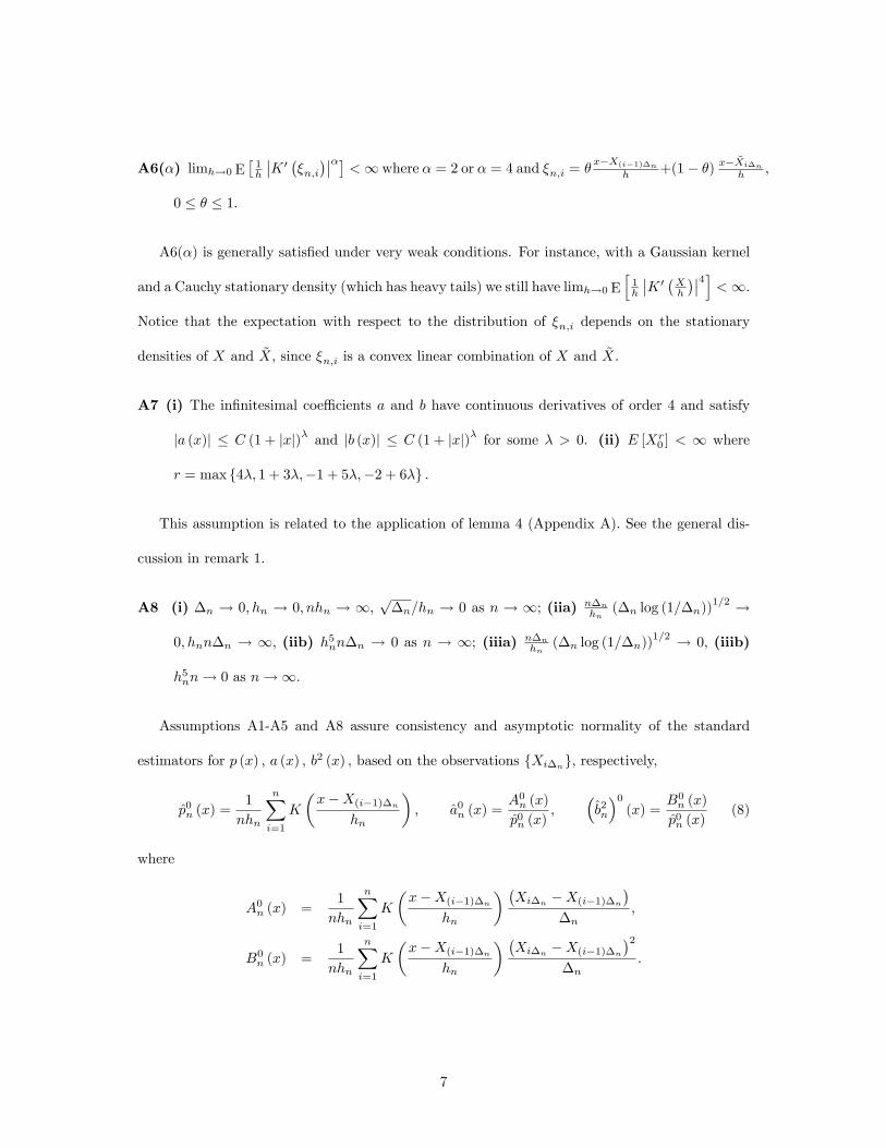
A6(�) limh!0 E�1h

��K 0 ��n;i����� <1 where � = 2 or � = 4 and �n;i = �x�X(i�1)�n

h +(1� �) x� ~Xi�n

h ,

0 � � � 1:

A6(�) is generally satis�ed under very weak conditions. For instance, with a Gaussian kernel

and a Cauchy stationary density (which has heavy tails) we still have limh!0 Eh1h

��K 0 �Xh

���4i <1.Notice that the expectation with respect to the distribution of �n;i depends on the stationary

densities of X and ~X; since �n;i is a convex linear combination of X and ~X.

A7 (i) The in�nitesimal coe¢ cients a and b have continuous derivatives of order 4 and satisfy

ja (x)j � C (1 + jxj)� and jb (x)j � C (1 + jxj)� for some � > 0. (ii) E [Xr0 ] < 1 where

r = max f4�; 1 + 3�;�1 + 5�;�2 + 6�g :

This assumption is related to the application of lemma 4 (Appendix A). See the general dis-

cussion in remark 1.

A8 (i) �n ! 0; hn ! 0; nhn ! 1;p�n=hn ! 0 as n ! 1; (iia) n�n

hn(�n log (1=�n))

1=2 !

0; hnn�n ! 1; (iib) h5nn�n ! 0 as n ! 1; (iiia) n�n

hn(�n log (1=�n))

1=2 ! 0; (iiib)

h5nn! 0 as n!1:

Assumptions A1-A5 and A8 assure consistency and asymptotic normality of the standard

estimators for p (x) ; a (x) ; b2 (x) ; based on the observations fXi�ng, respectively,

p0n (x) =1

nhn

nXi=1

K

�x�X(i�1)�n

hn

�; a0n (x) =

A0n (x)

p0n (x);

�b2n

�0(x) =

B0n (x)

p0n (x)(8)

where

A0n (x) =1

nhn

nXi=1

K

�x�X(i�1)�n

hn

� �Xi�n �X(i�1)�n

��n

;

B0n (x) =1

nhn

nXi=1

K

�x�X(i�1)�n

hn

� �Xi�n �X(i�1)�n

�2�n

:

7

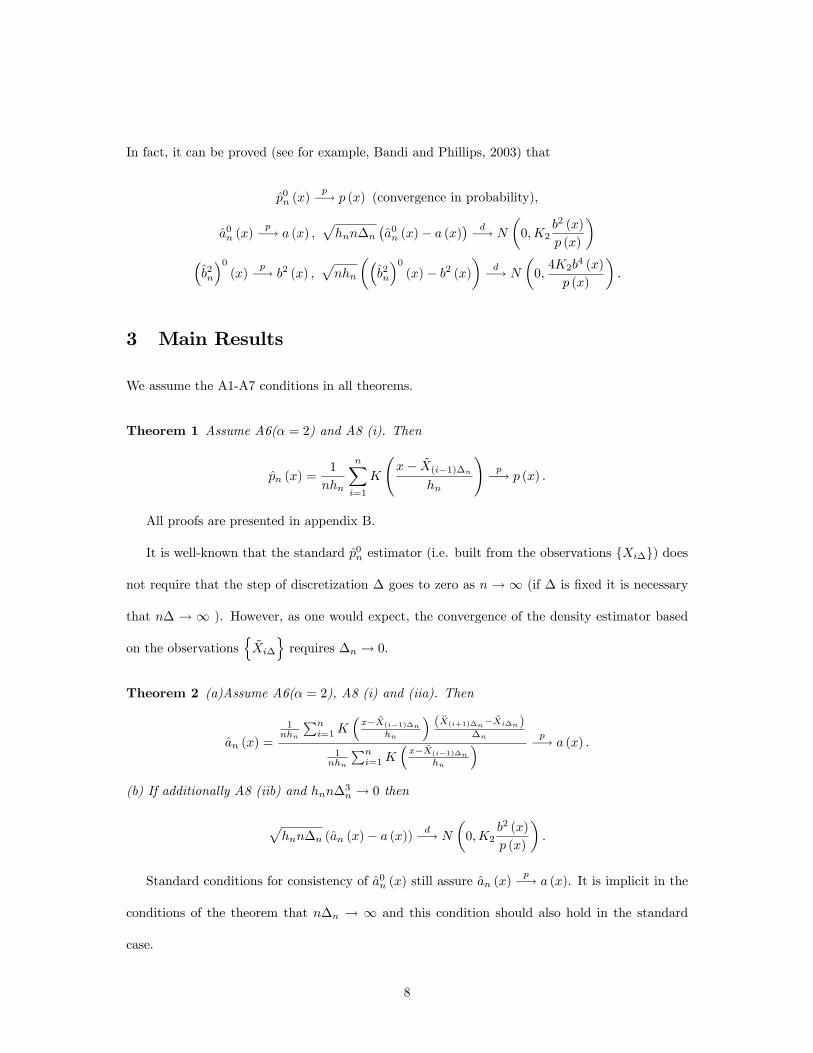
In fact, it can be proved (see for example, Bandi and Phillips, 2003) that

p0n (x)p�! p (x) (convergence in probability);

a0n (x)p�! a (x) ;

phnn�n

�a0n (x)� a (x)

� d�! N

�0;K2

b2 (x)

p (x)

��b2n

�0(x)

p�! b2 (x) ;pnhn

��b2n

�0(x)� b2 (x)

�d�! N

�0;4K2b

4 (x)

p (x)

�:

3 Main Results

We assume the A1-A7 conditions in all theorems.

Theorem 1 Assume A6(� = 2) and A8 (i). Then

pn (x) =1

nhn

nXi=1

K

x� ~X(i�1)�n

hn

!p�! p (x) :

All proofs are presented in appendix B.

It is well-known that the standard p0n estimator (i.e. built from the observations fXi�g) does

not require that the step of discretization � goes to zero as n ! 1 (if � is �xed it is necessary

that n� ! 1 ). However, as one would expect, the convergence of the density estimator based

on the observationsn~Xi�

orequires �n ! 0:

Theorem 2 (a)Assume A6(� = 2), A8 (i) and (iia). Then

an (x) =

1nhn

Pni=1K

�x� ~X(i�1)�n

hn

�( ~X(i+1)�n� ~Xi�n)

�n

1nhn

Pni=1K

�x� ~X(i�1)�n

hn

� p�! a (x) :

(b) If additionally A8 (iib) and hnn�3n ! 0 then

phnn�n (an (x)� a (x))

d�! N

�0;K2

b2 (x)

p (x)

�:

Standard conditions for consistency of a0n (x) still assure an (x)p�! a (x). It is implicit in the

conditions of the theorem that n�n ! 1 and this condition should also hold in the standard

case.

8

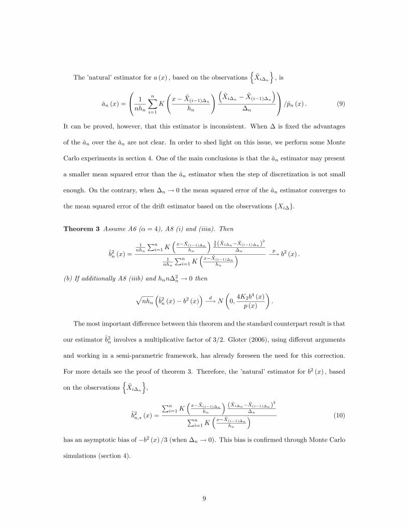
The �natural�estimator for a (x) ; based on the observationsn~Xi�n

o; is

�an (x) =

0@ 1

nhn

nXi=1

K

x� ~X(i�1)�n

hn

! � ~Xi�n� ~X(i�1)�n

��n

1A =pn (x) : (9)

It can be proved, however, that this estimator is inconsistent. When � is �xed the advantages

of the an over the �an are not clear. In order to shed light on this issue, we perform some Monte

Carlo experiments in section 4. One of the main conclusions is that the �an estimator may present

a smaller mean squared error than the an estimator when the step of discretization is not small

enough. On the contrary, when �n ! 0 the mean squared error of the an estimator converges to

the mean squared error of the drift estimator based on the observations fXi�g.

Theorem 3 Assume A6 (� = 4), A8 (i) and (iiia). Then

b2n (x) =

1nhn

Pni=1K

�x� ~X(i�1)�n

hn

� 32 ( ~Xi�n� ~X(i�1)�n)

2

�n

1nhn

Pni=1K

�x� ~X(i�1)�n

hn

� p�! b2 (x) :

(b) If additionally A8 (iiib) and hnn�2n ! 0 then

pnhn

�b2n (x)� b2 (x)

�d�! N

�0;4K2b

4 (x)

p (x)

�:

The most important di¤erence between this theorem and the standard counterpart result is that

our estimator b2n involves a multiplicative factor of 3=2. Gloter (2006), using di¤erent arguments

and working in a semi-parametric framework, has already foreseen the need for this correction.

For more details see the proof of theorem 3. Therefore, the �natural�estimator for b2 (x) ; based

on the observationsn~Xi�n

o,

b2n;� (x) =

Pni=1K

�x� ~X(i�1)�n

hn

�( ~Xi�n� ~X(i�1)�n)

2

�nPni=1K

�x� ~X(i�1)�n

hn

� (10)

has an asymptotic bias of �b2 (x) =3 (when �n ! 0). This bias is con�rmed through Monte Carlo

simulations (section 4).

9

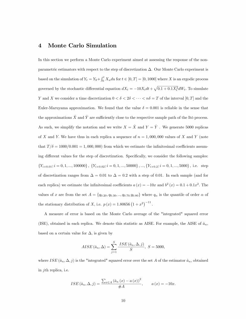
4 Monte Carlo Simulation

In this section we perform a Monte Carlo experiment aimed at assessing the response of the non-

parametric estimators with respect to the step of discretization �. Our Monte Carlo experiment is

based on the simulation of Yt = Y0+R t0Xudu for t 2 [0; T ] = [0; 1000] whereX is an ergodic process

governed by the stochastic di¤erential equation dXt = �10Xtdt+p0:1 + 0:1X2

t dWt: To simulate

Y and X we consider a time discretization 0 < � < 2� < � � � < n� = T of the interval [0; T ] and the

Euler-Maruyama approximation. We found that the value � = 0:001 is reliable in the sense that

the approximations X and Y are su¢ ciently close to the respective sample path of the Itô process.

As such, we simplify the notation and we write X = X and Y = Y . We generate 5000 replicas

of X and Y: We have thus in each replica a sequence of n = 1; 000; 000 values of X and Y (note

that T=� = 1000=0:001 = 1; 000; 000) from which we estimate the in�nitesimal coe¢ cients assum-

ing di¤erent values for the step of discretization. Speci�cally, we consider the following samples:

fYi�0:01; i = 0; 1; :::; 100000g ; fYi�0:02; i = 0; 1; :::; 50000g ; :::; fYi�0:2; i = 0; 1; :::; 5000g ; i.e. step

of discretization ranges from � = 0:01 to � = 0:2 with a step of 0:01. In each sample (and for

each replica) we estimate the in�nitesimal coe¢ cients a (x) = �10x and b2 (x) = 0:1+ 0:1x2: The

values of x are from the set A = fq0:20; q0:30; ::; q0:70;q0:80g where q� is the quantile of order � of

the stationary distribution of X; i.e. p (x) = 1:80656�1 + x2

��11:

A measure of error is based on the Monte Carlo average of the "integrated" squared error

(ISE), obtained in each replica. We denote this statistic as AISE. For example, the AISE of an;

based on a certain value for �; is given by

AISE (an;�) =SXj=1

ISE (an;�; j)

S; S = 5000;

where ISE (an;�; j) is the "integrated" squared error over the set A of the estimator an; obtained

in jth replica, i.e.

ISE (an;�; j) =

Px2A (an (x)� a (x))

2

#A; a (x) = �10x:

10

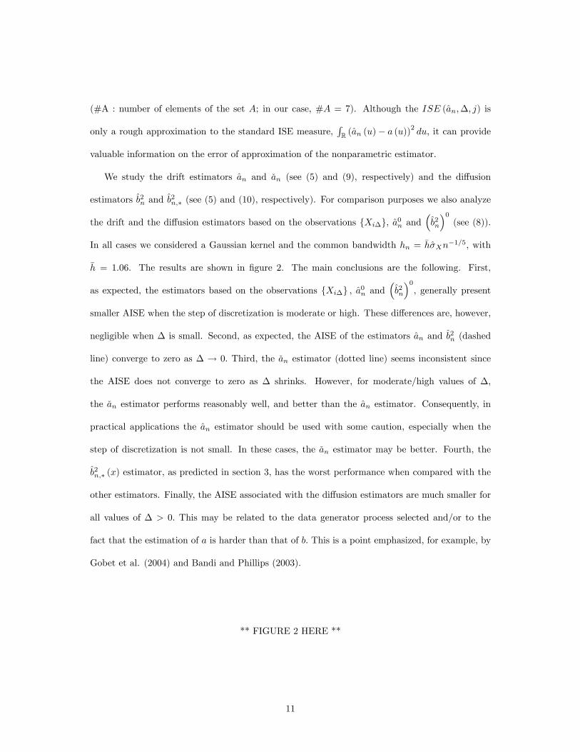
(#A : number of elements of the set A; in our case, #A = 7). Although the ISE (an;�; j) is

only a rough approximation to the standard ISE measure,RR (an (u)� a (u))

2du; it can provide

valuable information on the error of approximation of the nonparametric estimator.

We study the drift estimators an and �an (see (5) and (9), respectively) and the di¤usion

estimators b2n and b2n;� (see (5) and (10), respectively). For comparison purposes we also analyze

the drift and the di¤usion estimators based on the observations fXi�g, a0n and�b2n

�0(see (8)).

In all cases we considered a Gaussian kernel and the common bandwidth hn = �h�Xn�1=5, with

�h = 1:06. The results are shown in �gure 2. The main conclusions are the following. First,

as expected, the estimators based on the observations fXi�g ; a0n and�b2n

�0, generally present

smaller AISE when the step of discretization is moderate or high. These di¤erences are, however,

negligible when � is small. Second, as expected, the AISE of the estimators an and b2n (dashed

line) converge to zero as � ! 0: Third, the �an estimator (dotted line) seems inconsistent since

the AISE does not converge to zero as � shrinks. However, for moderate/high values of �;

the �an estimator performs reasonably well, and better than the an estimator. Consequently, in

practical applications the an estimator should be used with some caution, especially when the

step of discretization is not small. In these cases, the �an estimator may be better. Fourth, the

b2n;� (x) estimator, as predicted in section 3, has the worst performance when compared with the

other estimators. Finally, the AISE associated with the di¤usion estimators are much smaller for

all values of � > 0: This may be related to the data generator process selected and/or to the

fact that the estimation of a is harder than that of b: This is a point emphasized, for example, by

Gobet et al. (2004) and Bandi and Phillips (2003).

** FIGURE 2 HERE **

11

5 Conclusions and Other Extensions

In this article we showed that standard non-parametric estimators of the in�nitesimal coe¢ cients

of second order stochastic di¤erential equations, based on the observationsn~Xi�

o, are not appro-

priate, since they are inconsistent, even when �n ! 0: However, as shown, slight modi�cations to

the standard estimators allow us to de�ne consistent estimators.

There are some extensions that can be considered such as non-equidistant observations, optimal

bandwidth choice, data-driven estimation, minimax rates. More general assumptions on the data

generator process as in Bandi and Phillips (2003) can also be applied.

12

References

Aït-Sahalia, Y. (2002) Maximum Likelihood Estimation of Discretely Sampled Di¤usions: A

Closed-Form Approximation Approach. Econometrica 70(1), 223-262.

Arnold, L. (1974) Stochastic Di¤erential Equations: Theory And Application. John Wiley &

Sons.

Bandi, F. & P. Phillips (2003) Fully Nonparametric Estimation of Scalar Di¤usion Models.

Econometrica 71, 241-283.

Bibby, B. & M. Sørensen (1997) A Hyperbolic Di¤usion Model for Stock Prices. Finance and

Stochastics 1, 25-41.

Chen, X. & L. Hansen & M. Carrasco (1998) Nonlinearity and Temporal Dependence. Unpub-

lished.

Dacunha-Castelle, D. & Florens-Zmirou (1986) Estimation of the Coe¢ cient of a Di¤usion From

Discretely Sample Observations. Stochastic 19, 263-284.

Ditlevsen S. & M. Sørensen (2004) Inference for Observations of Integrated Di¤usion Processes.

Scandinavian Journal of Statistics 31(3), 417-429.

Florens-Zmirou, D. (1989) Approximate Discrete-Time Schemes for Statistics of Di¤usion Processes.

Statistics 4, 547-557.

Florens-Zmirou, D. (1993) On Estimating the Di¤usion Coe¢ cient from Discrete Observation.

Journal of Applied Probability 30, 790-804.

Gobet, E. & M. Ho¤mann & M. Reiß(2004) Nonparametric Estimation of Scalar Di¤usions

based on Low Frequency Data, Annals of Statistics 32(5), 2223�2253.

Gloter A. (2001) Parameter Estimation for a Discrete Sampling of an Integrated Ornstein-

Uhlenbeck Process. Statistics 35, 225-243.

13

Gloter A. (2006) Parameter Estimation for a Discretely Observed Integrated Di¤usion Process.

Scandinavian Journal of Statistics 33.

Hansen, L. & J. Scheinkman (1995) Back to the Future: Generating Moment Implications for

Continuous-Time Markov Processes. Econometrica 63, 767-804.

Jiang, G. & J. Knight (1997) A Nonparametric Approach to the Estimation of Di¤usion Processes,

with an Application to a Short-Term Interest Rate Model. Econometric Theory 13, 615-645.

Kessler M. (1997), Estimation of an Ergodic Di¤usion from Discrete Observations. Scandinavian

Journal of Statistics 24(2), 211- 229.

Nicolau J. (2003) Bias Reduction in Nonparametric Di¤usion Coe¢ cient Estimation. Econometric

Theory 19(5), 754-777.

Rao, B. (1983) Nonparametrical Functional Estimation. New York, Academic Press.

Skorokhod, A. (1989) Asymptotic Methods in the Theory of Stochastic Di¤erential Equation.

Translation of Mathematical Monographs 78, American Mathematical Society.

14

Appendix A: Auxiliary Results

In the following lemma we generalize a formula of Florens-Zmirou (1989) to multivariate dif-

fusions. Lemma 4 is essential in the proofs of all the theorems presented in this work.

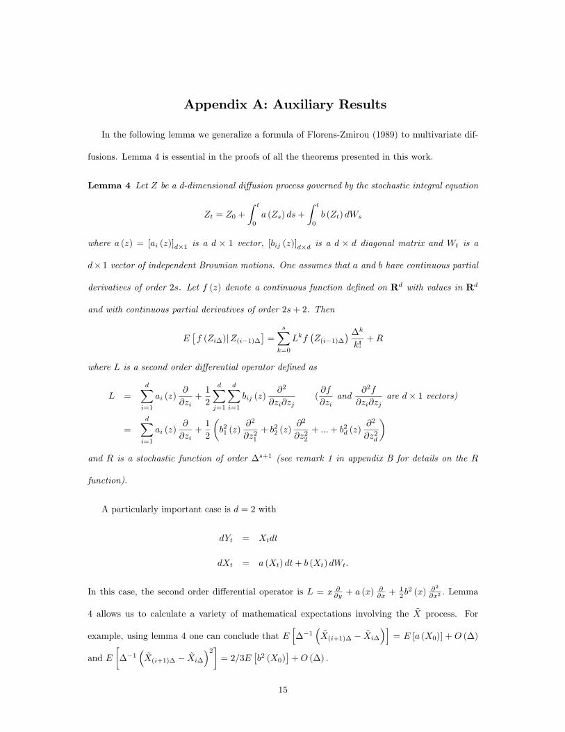
Lemma 4 Let Z be a d-dimensional di¤usion process governed by the stochastic integral equation

Zt = Z0 +

Z t

0

a (Zs) ds+

Z t

0

b (Zt) dWs

where a (z) = [ai (z)]d�1 is a d � 1 vector, [bij (z)]d�d is a d � d diagonal matrix and Wt is a

d� 1 vector of independent Brownian motions. One assumes that a and b have continuous partial

derivatives of order 2s. Let f (z) denote a continuous function de�ned on Rd with values in Rd

and with continuous partial derivatives of order 2s+ 2. Then

E�f (Zi�)jZ(i�1)�

�=

sXk=0

Lkf�Z(i�1)�

� �kk!+R

where L is a second order di¤erential operator de�ned as

L =dXi=1

ai (z)@

@zi+1

2

dXj=1

dXi=1

bij (z)@2

@zi@zj(@f

@ziand

@2f

@zi@zjare d� 1 vectors)

=dXi=1

ai (z)@

@zi+1

2

�b21 (z)

@2

@z21+ b22 (z)

@2

@z22+ :::+ b2d (z)

@2

@z2d

�and R is a stochastic function of order �s+1 (see remark 1 in appendix B for details on the R

function).

A particularly important case is d = 2 with

dYt = Xtdt

dXt = a (Xt) dt+ b (Xt) dWt:

In this case, the second order di¤erential operator is L = x @@y + a (x)

@@x +

12b2 (x) @2

@x2 : Lemma

4 allows us to calculate a variety of mathematical expectations involving the ~X process. For

example, using lemma 4 one can conclude that Eh��1

�~X(i+1)� � ~Xi�

�i= E [a (X0)] + O (�)

and E���1

�~X(i+1)� � ~Xi�

�2�= 2=3E

�b2 (X0)

�+O (�) :

15

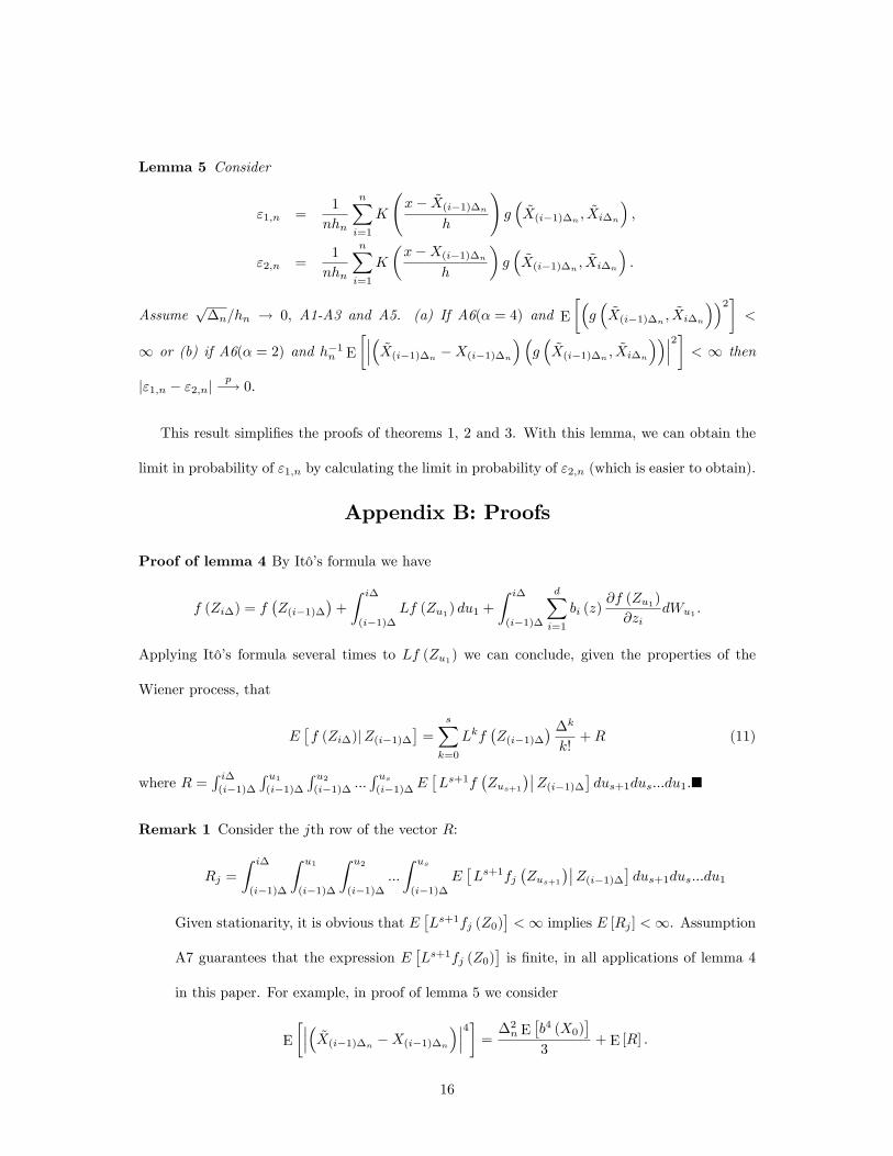
Lemma 5 Consider

"1;n =1

nhn

nXi=1

K

x� ~X(i�1)�n

h

!g�~X(i�1)�n

; ~Xi�n

�;

"2;n =1

nhn

nXi=1

K

�x�X(i�1)�n

h

�g�~X(i�1)�n

; ~Xi�n

�:

Assumep�n=hn ! 0; A1-A3 and A5. (a) If A6(� = 4) and E

��g�~X(i�1)�n

; ~Xi�n

��2�<

1 or (b) if A6(� = 2) and h�1n E

����� ~X(i�1)�n�X(i�1)�n

��g�~X(i�1)�n

; ~Xi�n

�����2� < 1 then

j"1;n � "2;njp�! 0:

This result simpli�es the proofs of theorems 1, 2 and 3. With this lemma, we can obtain the

limit in probability of "1;n by calculating the limit in probability of "2;n (which is easier to obtain).

Appendix B: Proofs

Proof of lemma 4 By Itô�s formula we have

f (Zi�) = f�Z(i�1)�

�+

Z i�

(i�1)�Lf (Zu1) du1 +

Z i�

(i�1)�

dXi=1

bi (z)@f (Zu1)

@zidWu1 :

Applying Itô�s formula several times to Lf (Zu1) we can conclude, given the properties of the

Wiener process, that

E�f (Zi�)jZ(i�1)�

�=

sXk=0

Lkf�Z(i�1)�

� �kk!+R (11)

where R =R i�(i�1)�

R u1(i�1)�

R u2(i�1)� :::

R us(i�1)�E

�Ls+1f

�Zus+1

���Z(i�1)�� dus+1dus:::du1:�Remark 1 Consider the jth row of the vector R:

Rj =

Z i�

(i�1)�

Z u1

(i�1)�

Z u2

(i�1)�:::

Z us

(i�1)�E�Ls+1fj

�Zus+1

���Z(i�1)�� dus+1dus:::du1Given stationarity, it is obvious that E

�Ls+1fj (Z0)

�<1 implies E [Rj ] <1. Assumption

A7 guarantees that the expression E�Ls+1fj (Z0)

�is �nite, in all applications of lemma 4

in this paper. For example, in proof of lemma 5 we consider

E

����� ~X(i�1)�n�X(i�1)�n

����4� = �2n E�b4 (X0)

�3

+ E [R] :

16

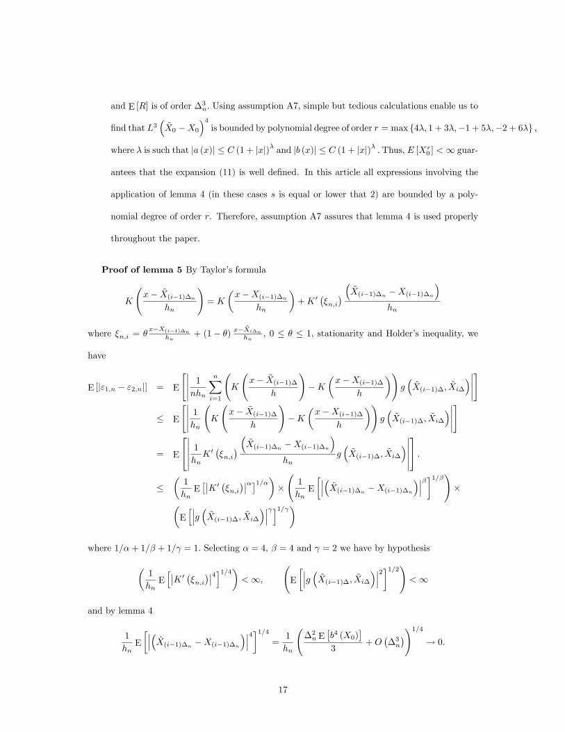
and E [R] is of order �3n: Using assumption A7, simple but tedious calculations enable us to

�nd that L3�~X0 �X0

�4is bounded by polynomial degree of order r = max f4�; 1 + 3�;�1 + 5�;�2 + 6�g ;

where � is such that ja (x)j � C (1 + jxj)� and jb (x)j � C (1 + jxj)� : Thus, E [Xr0 ] <1 guar-

antees that the expansion (11) is well de�ned. In this article all expressions involving the

application of lemma 4 (in these cases s is equal or lower that 2) are bounded by a poly-

nomial degree of order r. Therefore, assumption A7 assures that lemma 4 is used properly

throughout the paper.

Proof of lemma 5 By Taylor�s formula

K

x� ~X(i�1)�n

hn

!= K

�x�X(i�1)�n

hn

�+K 0 ��n;i�

�~X(i�1)�n

�X(i�1)�n

�hn

where �n;i = �x�X(i�1)�n

hn+ (1� �) x� ~Xi�n

hn, 0 � � � 1; stationarity and Holder�s inequality, we

have

E [j"1;n � "2;nj] = E

"����� 1nhnnXi=1

K

x� ~X(i�1)�

h

!�K

�x�X(i�1)�

h

�!g�~X(i�1)�; ~Xi�

������#

� E

"����� 1hn K

x� ~X(i�1)�

h

!�K

�x�X(i�1)�

h

�!g�~X(i�1)�; ~Xi�

������#

= E

24������ 1hnK 0 ��n;i��~X(i�1)�n

�X(i�1)�n

�hn

g�~X(i�1)�; ~Xi�

�������35 :

��1

hnE���K 0 ��n;i�����1=���

1

hnE

����� ~X(i�1)�n�X(i�1)�n

������1=�!��Eh���g � ~X(i�1)�; ~Xi����� i1= �

where 1=�+ 1=� + 1= = 1: Selecting � = 4; � = 4 and = 2 we have by hypothesis

�1

hnEh��K 0 ��n;i���4i1=4� <1;

E

����g � ~X(i�1)�; ~Xi�����2�1=2!<1

and by lemma 4

1

hnE

����� ~X(i�1)�n�X(i�1)�n

����4�1=4 = 1

hn

�2n E

�b4 (X0)

�3

+O��3n�!1=4

! 0:

17

Thus E [j"1;n � "2;nj]! 0: Part (b) is immediate from Chauchy-Schwarz inequality (in this case it

is su¢ cient to consider limh!0 Eh1h

��K 0 ��n;i���2i <1).�Proof of theorem 1 Let

p0n (x) =1

nhn

nXi=1

K

�x�X(i�1)�n

hn

�:

It is well known that under the conditions of the theorem one has

E���p0n (x)� p (x)���! 0

(see, for example, Bandi and Phillips, 2003). It remains to show that E���pn (x)� p0n (x)��� ! 0.

This follows immediately from lemma 5 (b) with g � 1: Therefore, the right-hand side of the

inequality

E [jpn (x)� p (x)j] � E���pn (x)� p0n (x)���+ E ���p0n (x)� p (x)���

goes to zero (under the conditions of the theorem). Thus, we have E [jpn (x)� p (x)j]! 0 and, by

Chebyshev�s inequality, pn (x)p�! p (x) :�

Proof of theorem 2 (a) From the proof of theorem 1 we know that pn (x)p�! p (x) : Thus,

to prove an (x) = An (x) =pn (x)p�! a (x) it is su¢ cient to verify that An (x)

p�! a (x) p (x) : Let

us consider

A0n (x) =1

nhn

nXi=1

K

�x�X(i�1)�n

hn

� �Xi�n

�X(i�1)�n

��n

:

Under the conditions of the theorem it is known that A0n (x)p�! a (x) p (x) (see Bandi and Phillips,

2003). The idea is to prove that An (x)�A0n (x)p�! 0 which implies that An (x)

p�! a (x) p (x) and

consequently an (x)p�! a (x) : By lemma 5 (b) An (x)� A0n (x) has the same limit in probability

as

�1;n =1

nhn

nXi=1

K

�x�X(i�1)�n

hn

� � ~X(i+1)�n� ~Xi�n

��n

� 1

nhn

nXi=1

K

�x�X(i�1)�n

hn

� �Xi�n �X(i�1)�n

��n

=1

nhn

nXi=1

K

�x�X(i�1)�n

hn

�0@�~X(i+1)�n

� ~Xi�n

��n

��Xi�n

�X(i�1)�n

��n

1A :18

We now show that �1;n (x)p�! 0: By lemma 4, A7 and stationarity, we have

E [�1;n (x)]

= E

24 1hnK

�x�X(i�1)�n

hn

�0@�~X(i+1)�n

� ~Xi�n

��n

��Xi�n

�X(i�1)�n

��n

1A35= E

24 1hnK

�x�X(i�1)�n

hn

�E

24E240@

�~X(i+1)�n

� ~Xi�n

��n

��Xi�n �X(i�1)�n

��n

1A������Fi�n

35������F(i�1)�n

3535=

�n2E

�1

hnK

�x�X(i�1)�n

hn

��a�X(i�1)�n

�a0�X(i�1)�n

�+1

2b2�X(i�1)�n

�a00�X(i�1)�n

���=

�n2

Z1

hnK

�x� uhn

��a (u) a0 (u) +

1

2b2 (u) a00 (u)

�p (u) du

= O (�n) :

On the other hand,

V ar [�1;n (x)]

=1

n�nhnV ar

26666641pn

nXi=1

1phnK

�x�X(i�1)�n

hn

�p�n

0@�~X(i+1)�n

� ~Xi�n

��n

��Xi�n

�X(i�1)�n

��n

1A| {z }

gi

3777775=

1

n�nhnV ar

"1pn

nXi=1

gi

#:

We have V arh1pn

Pni=1 gi

i= 1

n

Pni=1 E

h1hK

2�x�X(i�1)�n

hn

�f2i+ n where n represents the

sum of 2nPn�1

j=1

Pni=j+1 terms involving the autocovariances. Under stationarity and assumption

A4 (X and ~X are � - mixing and � - mixing), the jth autocovariance of gi tends to zero at

exponential rate as j !1, for all functions g such that E�g2i�<1: Therefore, if E

�g2i�<1; the

series 1 is absolutely convergent and one has V arh1pn

Pni=1 gi

i< 1: Since

RK2 (u) du < 1

and X has stationary density, one can conclude that

E�g2i�= E

264 1hnK2

�x�X(i�1)�n

hn

��n

0@�~X(i+1)�n

� ~Xi�n

��n

��Xi�n �X(i�1)�n

��n

1A2375

is �nite since, by lemma 4,

E

264�n0@�~X(i+1)�n

� ~Xi�n

��n

��Xi�n

�X(i�1)�n

��n

1A2375 = 2

3E�b2 (X0)

�+O (�n) :

19

In conclusion, V ar [�1;n (x)] = 1n�nhn

V arh1pn

Pni=1 gi

i! 0 as n�nhn !1:

(b) By hypothesis (see Bandi and Phillips, 2003)

Z0n (x) =phnn�n

�a0n (x)� a (x)

� d�! N

�0;K2

b2 (x)

p (x)

�(12)

where a0n (x) = A0n (x) =pn (x). By the asymptotic equivalence theorem, it su¢ ces to prove that

Zn (x)� Z0n (x)p�! 0 where Zn (x) =

phnn�n (an (x)� a (x)) : From part (a) we know that

Zn (x)� Z0n (x) =phnn�n

��1;n (x)

pn (x)

�

and �1;n (x) =pn (x) = Op (�n) : Thus, under the assumption hnn�3n ! 0; the results holds.�

Proof of theorem 3 (a) From the proof of theorem 1 we know that pn (x)p�! p (x) : Thus, to

prove b2n (x) = Bn (x) =pn (x)p�! b2 (x) it is su¢ cient to verify that Bn (x)

p�! b2 (x) p (x) : Let

us consider

B0n (x) =1

nhn

nXi=1

K

�x�X(i�1)�n

hn

� �Xi�n

�X(i�1)�n

�2�n

:

Under the conditions of the theorem it is known that B0n (x)p�! b2 (x) p (x) (see Bandi and

Phillips, 2003). The idea is to prove that Bn (x) � B0n (x)p�! 0 which implies that Bn (x)

p�!

b2 (x) p (x) and consequently b2n (x)p�! b2 (x) : By lemma 5 (a) Bn (x)�B0n (x) has the same limit

in probability as

�2;n (x) =1

nhn

nXi=1

K

�x�X(i�1)�n

hn

� 32

�~Xi�n

� ~X(i�1)�n

�2�n

� 1

nhn

nXi=1

K

�x�X(i�1)�n

hn

� �Xi�n

�X(i�1)�n

�2�n

=1

nhn

nXi=1

K

�x�X(i�1)�n

hn

�0B@ 32

�~Xi�n

� ~X(i�1)�n

�2�n

��Xi�n �X(i�1)�n

�2�n

1CA :We now prove that �2;n (x)

p�! 0. Let us consider

�3;n (x) =1

nhn

nXi=1

K

�x�X(i�1)�n

hn

�fi

20

where fi =�

32 ( ~Xi�n� ~X(i�1)�n)

2

�n� (Xi�n�X(i�1)�n)

2

�n

�: Since, by lemma 4

E

264E264 32

�~Xi�n

� ~X(i�1)�n

�2�n

�������Fi�n

375�������F(i�1)�n

375 = b2�X(i�1)�n

�+O (�n) :

E

" �Xi�n

�X(i�1)�n

�2�n

�����Fi�n

#= b2

�X(i�1)�n

�+O (�n) :

one has

E [fi] = E

2640B@ 3

2

�~Xi�n � ~X(i�1)�n

�2�n

��Xi�n

�X(i�1)�n

�2�n

1CA375 = O (�n) :

On the other hand,

V ar [�2;n (x)]

=1

nhnV ar

266666641pn

nXi=1

1phnK

�x�X(i�1)�n

hn

�0B@ 32

�~Xi�n

� ~X(i�1)�n

�2�n

��Xi�n

�X(i�1)�n

�2�n

1CA| {z }

gi

37777775=

1

nhnV ar

"1pn

nXi=1

gi

#:

Using the same arguments as in the proof of theorem 2 (a), it is easy to conclude that the condition

E

26640B@ 3

2

�~Xi�n � ~X(i�1)�n

�2�n

��Xi�n

�X(i�1)�n

�2�n

1CA23775 = O (1)

assures V ar [�2;n (x)]! 0:

(b) By hypothesis (see Bandi and Phillips, 2003)

Z0n (x) =pnhn

��b2n

�0(x)� b2 (x)

�d�! N

�0;4K2b

4 (x)

p (x)

�where

�b2n

�0(x) = B0n (x) =pn (x). By the asymptotic equivalence theorem it is su¢ cient to prove

that Zn (x)� Z0n (x)p�! 0 where Zn (x) =

pnhn

�b2n (x)� b2 (x)

�: From part (a) we know that

Zn (x)� Z0n (x) =pnhn

�2;n (x)

pn (x):

and �3;n (x) = Op (�n) : Thus, under the assumption hnn�2n ! 0 the results holds.�

21

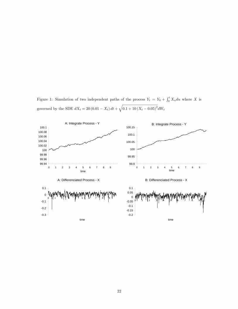
Figure 1: Simulation of two independent paths of the process Yt = Y0 +R t0Xudu where X is

governed by the SDE dXt = 20 (0:01�Xt) dt+q0:1 + 10 (Xt � 0:05)2dWt

A: Integrate Process ­ Y

99.9499.9699.98

100100.02100.04100.06100.08100.1

0 1 2 3 4 5 6 7 8 9time

A: Differenciated Process ­ X

­0.3

­0.2

­0.1

0

0.1

0 1 2 3 4 5 6 7 8 9

time

B: Integrate Process ­ Y

99.9

99.95

100

100.05

100.1

100.15

0 1 2 3 4 5 6 7 8 9time

B: Differenciated Process ­ X

­0.2­0.15

­0.1­0.05

00.05

0.1

0 1 2 3 4 5 6 7 8 9

time

22

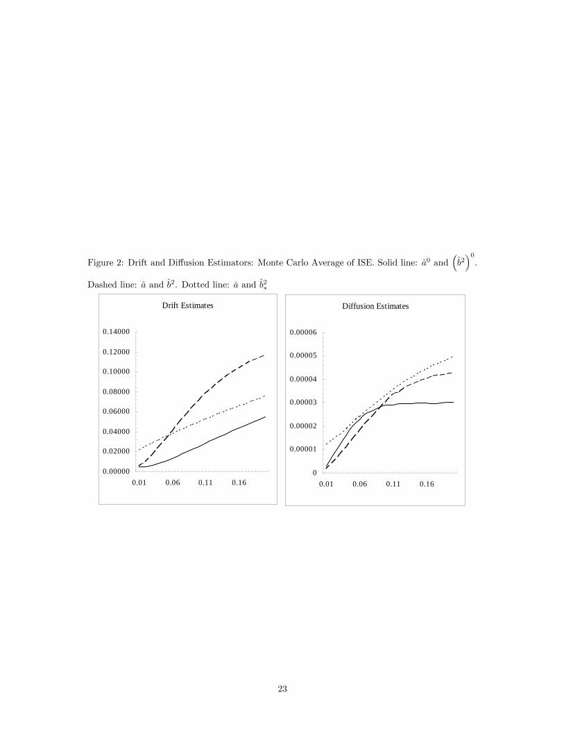
Figure 2: Drift and Di¤usion Estimators: Monte Carlo Average of ISE. Solid line: a0 and�b2�0.

Dashed line: a and b2. Dotted line: �a and b2�

Drift Estimates

0.00000

0.02000

0.04000

0.06000

0.08000

0.10000

0.12000

0.14000

0.01 0.06 0.11 0.16

Diffusion Estimates

0

0.00001

0.00002

0.00003

0.00004

0.00005

0.00006

0.01 0.06 0.11 0.16

23