Embed Size (px)
Citation preview

J. Fluid Mech. (2006), vol. 569, pp. 409–445. c© 2006 Cambridge University Press
doi:10.1017/S0022112006002916 Printed in the United Kingdom
409
Non-Oberbeck–Boussinesq effects in stronglyturbulent Rayleigh–Benard convection
By GUENTER AHLERS1, ERIC BROWN1,FRANCISCO FONTENELE ARAUJO2,
DENIS FUNFSCHILLING1, S IEGFRIED GROSSMANN3
AND DETLEF LOHSE2
1Department of Physics and iQCD, University of California, Santa Barbara, CA 93106,2Department of Science and Technology and J. M. Burgers Centre for Fluid Dynamics,
University of Twente, P. O. Box 217, 7500 AE Enschede, The Netherlands,3Fachbereich Physik der Philipps-Universitaet, Renthof 6, D-35032 Marburg, Germany
(Received 27 July 2005 and in revised form 18 June 2006)
Non-Oberbeck–Boussinesq (NOB) effects on the Nusselt number Nu and Reynoldsnumber Re in strongly turbulent Rayleigh–Benard (RB) convection in liquids wereinvestigated both experimentally and theoretically. In the experiments the heat current,the temperature difference, and the temperature at the horizontal midplane weremeasured. Three cells of different heights L, all filled with water and all withaspect ratio Γ close to 1, were used. For each L, about 1.5 decades in Ra werecovered, together spanning the range 108 � Ra � 1011. For the largest temperaturedifference between the bottom and top plates, ∆ =40 K, the kinematic viscosity andthe thermal expansion coefficient, owing to their temperature dependence, variedby more than a factor of 2. The Oberbeck–Boussinesq (OB) approximation oftemperature-independent material parameters thus was no longer valid. The ratioχ of the temperature drops across the bottom and top thermal boundary layersbecame as small as χ =0.83, which may be compared with the ratio χ = 1 inthe OB case. Nevertheless, the Nusselt number Nu was found to be only slightlysmaller (by at most 1.4%) than in the next larger cell with the same Rayleighnumber, where the material parameters were still nearly height independent. TheReynolds numbers in the OB and NOB case agreed with each other within theexperimental resolution of about 2%, showing that NOB effects for this parameterwere small as well. Thus Nu and Re are rather insensitive against even significantdeviations from OB conditions. Theoretically, we first account for the robustnessof Nu with respect to NOB corrections: the NOB effects in the top boundarylayer cancel those which arise in the bottom boundary layer as long as they arelinear in the temperature difference ∆. The net effects on Nu are proportional to∆2 and thus increase only slowly and still remain minor despite drastic material-parameter changes. We then extend the Prandtl–Blasius boundary-layer theoryto NOB Rayleigh–Benard flow with temperature-dependent viscosity and thermaldiffusivity. This allows calculation of the shift in the bulk temperature, the temperaturedrops across the boundary layers, and the ratio χ without the introduction ofany fitting parameter. The calculated quantities are in very good agreement withexperiment. When in addition we use the experimental finding that for water the sumof the top and bottom thermal boundary-layer widths (based on the slopes of thetemperature profiles at the plates) remains unchanged under NOB effects within theexperimental resolution, the theory also gives the measured small Nusselt-numberreduction for the NOB case. In addition, it predicts an increase by about 0.5%
410 G. Ahlers and others
of the Reynolds number, which is also consistent with the experimental data. Bystudying theoretically hypothetical liquids for which only one of the materialparameters is temperature dependent, we are able to shed further light on theorigin of NOB corrections in water: while the NOB deviation of χ from its OBvalue χ = 1 mainly originates from the temperature dependence of the viscosity, theNOB correction of the Nusselt number primarily originates from the temperaturedependence of the thermal diffusivity. Finally, we give predictions from our theoryfor the NOB corrections if glycerol were used as the operating liquid.
1. IntroductionControlled experiments on Rayleigh–Benard (RB) convection are normally done
with relatively small temperature differences ∆ between the top and the bottomplate, so that the Oberbeck–Boussinesq (OB) approximation can be used. Thatapproximation assumes that material properties such as the kinematic viscosity ν, thethermal diffusivity κ , the heat conductivity Λ, the isobaric specific heat capacity cp ,and the isobaric thermal expansion coefficient β can be considered to be temperatureindependent and thus to have constant values all over the cell (Oberbeck 1879;Boussinesq 1903). However, in order to achieve large Rayleigh numbers Ra, onewould like to make ∆ as large as possible. A relatively well-analysed effect dueto deviations from OB conditions is that the temperature drops across the topand bottom thermal boundary layers (Wu & Libchaber 1991; Zhang, Childress &Libchaber 1997) become different, i.e. an asymmetry with respect to the midplane ofthe cell shows up. The associated NOB effects on the Nusselt number Nu and theReynolds number Re are unclear. Nonetheless, it is often argued in very general termsthat NOB effects are responsible for some measured large-Ra peculiarities in Nu orRe. The lack of our understanding of possible NOB effects at large Ra on Nu and Remeasurements is all the more unsatisfactory, as it is in this large-Ra regime where thecrossover to an ultimate scaling regime Nu ∼ Ra1/2 is expected (Kraichnan 1962). Inhelium gas beyond Ra ≈ 1011 Chavanne et al. (1997, 2001) found a steeper increasein the logarithmic slope of the Nu(Ra) curve than Niemela et al. (2000, 2001) andthey associated this finding with the ultimate Kraichnan regime. However, there is amajor controversy about whether these and other large-Ra data are ‘contaminated’by NOB effects (Chavanne et al. 1997, 2001; Roche et al. 2001, 2002; Niemela et al.2000, 2001; Niemela & Sreenivasan 2003; Ashkenazi & Steinberg 1999).
The aim of this paper is first to present systematic measurements of NOB effects onthe Nusselt number Nu, the Reynolds number Re, and the centre temperature Tc ofthe cell and then to attempt to understand these NOB effects theoretically. We do soby extending the Prandtl–Blasius boundary-layer theory to the case of temperature-dependent viscosity and thermal diffusivity and apply this to NOB Rayleigh–Benardflow. Our results hold for liquids whose specific heat capacity cp and density ρ exceptfor buoyancy are temperature independent in sufficiently good approximation and ifthe flow is incompressible.
For small Ra close to the transition to convection and pattern formation, NOBeffects have been treated theoretically by various authors, and most systematicallyby Busse (1967). They were examined experimentally by Hoard, Robertson & Acrivos(1970); Ahlers (1980); Walden & Ahlers (1981); Ciliberto, Pampaloni & Perez-Garcia
Non-Oberbeck–Boussinesq effects in Rayleigh–Benard convection 411
(1988); Bodenschatz et al. (1991); Pampaloni et al. (1992); and were reviewed byBodenschatz, Pesch & Ahlers (2000).
The outline of the paper is as follows. In § 2 we introduce our notation anddefine quantitative measures of NOB effects. These include different thicknesses ofthe thermal boundary layers (BLs) as well as different temperature drops across theselayers at the bottom and the top plates. In § 3 we present our experimental resultsfor the various measures of NOB effects, in particular for Nu and Re. We find arobustness of Nu and Re towards NOB effects, which we try to rationalize in § 4. In§ 5 we briefly review the model of Wu & Libchaber (1991) and Zhang et al. (1997),who analysed NOB effects on RB flow for cryogenic helium gas and for glycerin, bothexperimentally and theoretically. We compare the predictions of their model with ourdata for water. Although they correctly predict the robustness of Nu with respect toNOB effects and even account for the very small Nu decrease for the NOB case, itturns out that a basic assumption of this model is not fulfilled. In § 6 we apply anextended Prandtl–Blasius boundary-layer theory to the NOB Rayleigh–Benard flow,gaining excellent agreement with the measured data for the centre temperature, theNusselt number, and the Reynolds number. § 7 contains the conclusions.
2. Characterization of non-Oberbeck–Boussinesq effects2.1. Control parameters
What fluid properties should be used to define the non-dimensional numbers ofnon-Oberbeck–Boussinesq Rayleigh–Benard flow? Since the commonly used controlparameters are the temperatures Tb and Tt at the bottom and top plates, the immediatechoice of a reference temperature to characterize the typical material properties is themean temperature Tm =(Tt + Tb)/2. The overall temperature drop is ∆ = Tb − Tt . Thecorresponding definition of the parameters describing the thermal convection is theRayleigh number
Ram =βmg∆L3
νmκm
≡ Ra, (2.1)
the Prandtl number
Prm = νm/κm ≡ Pr, (2.2)
and, as a response of the system, the Reynolds number of the resulting large-scalecirculation (the ‘wind’),
Rem =UL
νm
≡ Re. (2.3)
Here U is the mean velocity of the large-scale wind in the bulk of the fluid. Weassume that there is only one such velocity scale, or, to be more precise, that thevelocity of the wind is the same close to the top and close to the bottom of the cell.The label m indicates that the material parameters are those at the mean temperatureTm. In the following we shall omit the label m of Ra, Pr , Re, and, later, also of theNusselt number Nu. Whenever these non-labelled dimensionless parameters are used,the respective material properties are meant as those at the mean temperature Tm ofthe external control temperatures. The actual time-averaged temperature in the bulkis called Tc. It is different from Tm due to NOB effects: Tc �= Tm.
The notation used in this paper is shown in figure 1. The fluid properties such asν, κ , and β carry the same index as the corresponding temperature at which they areconsidered, e.g. νt = ν(Tt ) for the kinematic viscosity at the top plate, and so on.
412 G. Ahlers and others
Tm Tc
Tm TcTt
Tt
NOBOB
λt
λbλOB
λOB
Tb
Tb
∆t
∆b
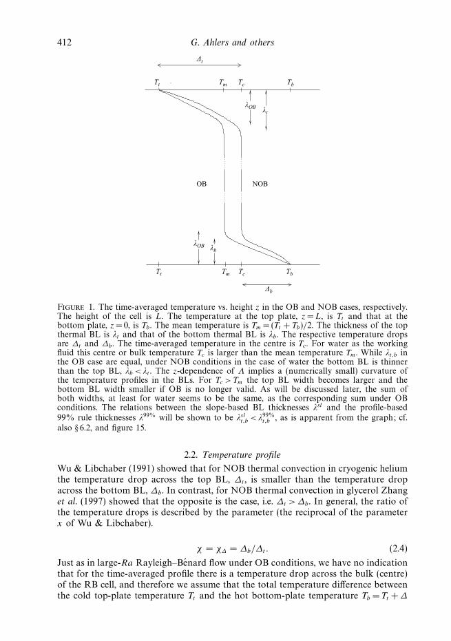
Figure 1. The time-averaged temperature vs. height z in the OB and NOB cases, respectively.The height of the cell is L. The temperature at the top plate, z = L, is Tt and that at thebottom plate, z = 0, is Tb . The mean temperature is Tm = (Tt + Tb)/2. The thickness of the topthermal BL is λt and that of the bottom thermal BL is λb . The respective temperature dropsare ∆t and ∆b . The time-averaged temperature in the centre is Tc . For water as the workingfluid this centre or bulk temperature Tc is larger than the mean temperature Tm. While λt,b inthe OB case are equal, under NOB conditions in the case of water the bottom BL is thinnerthan the top BL, λb < λt . The z-dependence of Λ implies a (numerically small) curvature ofthe temperature profiles in the BLs. For Tc >Tm the top BL width becomes larger and thebottom BL width smaller if OB is no longer valid. As will be discussed later, the sum ofboth widths, at least for water seems to be the same, as the corresponding sum under OBconditions. The relations between the slope-based BL thicknesses λsl and the profile-based99% rule thicknesses λ99% will be shown to be λsl
t,b < λ99%t,b , as is apparent from the graph; cf.
also § 6.2, and figure 15.
2.2. Temperature profile
Wu & Libchaber (1991) showed that for NOB thermal convection in cryogenic heliumthe temperature drop across the top BL, ∆t , is smaller than the temperature dropacross the bottom BL, ∆b. In contrast, for NOB thermal convection in glycerol Zhanget al. (1997) showed that the opposite is the case, i.e. ∆t >∆b. In general, the ratio ofthe temperature drops is described by the parameter (the reciprocal of the parameterx of Wu & Libchaber).
χ = χ∆ = ∆b/∆t . (2.4)
Just as in large-Ra Rayleigh–Benard flow under OB conditions, we have no indicationthat for the time-averaged profile there is a temperature drop across the bulk (centre)of the RB cell, and therefore we assume that the total temperature difference betweenthe cold top-plate temperature Tt and the hot bottom-plate temperature Tb = Tt +∆

Non-Oberbeck–Boussinesq effects in Rayleigh–Benard convection 413
consists only of the temperature drops across the thermal boundary layers,
∆ = ∆t + ∆b. (2.5)
The time-averaged temperature in the centre of the cell is then Tc = Tt + ∆t = Tb − ∆b.It deviates from Tm and expresses the response of the system to the NOB effects;Tm is just the arithmetic mean of the external control parameters. Depending on thefluid, Tc may be larger or smaller than Tm.
Equations (2.4) and (2.5) can be solved for the temperature drops ∆b and ∆t acrossthe bottom and top thermal BLs,
∆b =χ
1 + χ∆, (2.6)
∆t =1
1 + χ∆. (2.7)
The temperature profile in the container is shown in figure 1. In § 6 it will be calculatedwithin an extended Prandtl–Blasius boundary-layer theory.
2.3. Heat flux
The heat flux can be evaluated from the local heat-conservation equation
ρcp(∂tθ + ui∂iθ) = ∂i(Λ∂iθ), (2.8)
where θ is the temperature deviation from a convenient reference temperature, e.g.Tm. ∂i means ∂/∂xi , i = x, y, z are the three coordinates, and summation over repeatedindices is assumed. By starting from (2.8) we have already assumed that to a goodapproximation the variation in the entropy per mass s with pressure p does notcontribute, more precisely that∣∣∣∣dT
dz
∣∣∣∣ �∣∣∣∣ T
cp
(∂s
∂p
)T
dp
dz
∣∣∣∣.Using dp/dz = −ρg, the right-hand side of this inequality can be rewritten asρg(∂T /∂p)s ≡ ag . Thus we assume that ag , the adiabatic temperature change with pres-sure, is much smaller than the applied temperature gradient ∆/L (Furukawa & Onuki2002; Gitterman 1978; Landau & Lifshitz 1987). Indeed, for the experiment withwater described in § 3 we typically have agL/∆ ≈ 10−6 for this so-called Schwarzschildparameter, i.e. it is negligibly small. Note that for gases close to the critical point theSchwarzschild correction in general cannot be neglected (Gitterman & Steinberg 1971;Gitterman 1978; Ashkenazi & Steinberg 1999; Kogan & Meyer 2001; Furukawa &Onuki 2002).
We area-and-time-average (2.8); see (2.9). The label A indicates the planes z =constant, which are parallel to the top and bottom plates of the container. In addition,we assume that plane-averaged products of the type 〈ρcp∂z(uzθ)〉A or 〈Λ∂zθ〉A can beapproximated by their respective factorizations 〈ρcp〉A〈∂z(uzθ)〉A and 〈Λ〉A∂z〈θ〉A. Wethen obtain
∂z[〈ρcp〉A〈uzθ〉A − Λ(z)∂z〈θ〉A] = 〈uzθ〉A∂z〈ρcp〉A ≈ 0. (2.9)
In the second (approximate) equality, ≈, we have used the fact that for liquids the massdensity ρ and the isobaric specific heat capacity cp per mass to a good approximationare temperature, and therefore height, independent. For the case of water between 20and 60 ◦C, on which we will focus, these are given with precisions of 1.6% and 0.07%,respectively; see table 1. Thus in the following we will always consider ρ and cp as
414 G. Ahlers and others
temperature 10−3ρ 10−3cp 104β Λ 106κ 106ν P r
(◦C) (kg m−3) (J kg−1K−1) (K−1) (Wm−1K−1) (m2s−1) (m2s−1)
Tt = 20.000 0.99809 4.175 2.05 0.5975 0.1448 1.004 6.94Tt = 30.911 0.99532 4.169 3.14 0.6162 0.1494 0.794 5.31Tm = 40.000 0.99220 4.169 3.88 0.6297 0.1528 0.669 4.38Tc = 41.822 0.99150 4.169 4.02 0.6322 0.1534 0.648 4.23Tb = 50.911 0.98761 4.173 4.64 0.6434 0.1563 0.557 3.57Tb = 60.000 0.98316 4.178 5.21 0.6529 0.1590 0.485 3.05
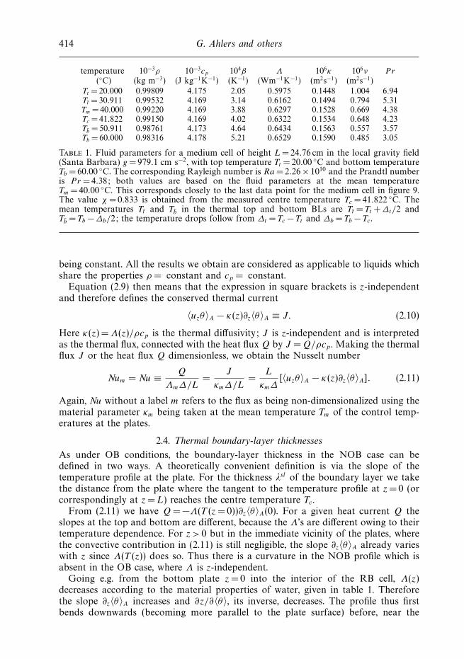
Table 1. Fluid parameters for a medium cell of height L =24.76 cm in the local gravity field(Santa Barbara) g = 979.1 cm s−2, with top temperature Tt = 20.00 ◦C and bottom temperatureTb = 60.00 ◦C. The corresponding Rayleigh number is Ra = 2.26 × 10¹⁰ and the Prandtl numberis Pr = 4.38; both values are based on the fluid parameters at the mean temperatureTm = 40.00 ◦C. This corresponds closely to the last data point for the medium cell in figure 9.The value χ = 0.833 is obtained from the measured centre temperature Tc =41.822 ◦C. Themean temperatures Tt and Tb in the thermal top and bottom BLs are Tt = Tt + ∆t/2 andTb = Tb − ∆b/2; the temperature drops follow from ∆t = Tc − Tt and ∆b = Tb − Tc .
being constant. All the results we obtain are considered as applicable to liquids whichshare the properties ρ = constant and cp = constant.
Equation (2.9) then means that the expression in square brackets is z-independentand therefore defines the conserved thermal current
〈uzθ〉A − κ(z)∂z〈θ〉A ≡ J. (2.10)
Here κ(z) = Λ(z)/ρcp is the thermal diffusivity; J is z-independent and is interpretedas the thermal flux, connected with the heat flux Q by J = Q/ρcp . Making the thermalflux J or the heat flux Q dimensionless, we obtain the Nusselt number
Num = Nu ≡ Q
Λm∆/L=
J
κm∆/L=
L
κm∆[〈uzθ〉A − κ(z)∂z〈θ〉A]. (2.11)
Again, Nu without a label m refers to the flux as being non-dimensionalized using thematerial parameter κm being taken at the mean temperature Tm of the control temp-eratures at the plates.
2.4. Thermal boundary-layer thicknesses
As under OB conditions, the boundary-layer thickness in the NOB case can bedefined in two ways. A theoretically convenient definition is via the slope of thetemperature profile at the plate. For the thickness λsl of the boundary layer we takethe distance from the plate where the tangent to the temperature profile at z = 0 (orcorrespondingly at z = L) reaches the centre temperature Tc.
From (2.11) we have Q = −Λ(T (z =0))∂z〈θ〉A(0). For a given heat current Q theslopes at the top and bottom are different, because the Λ’s are different owing to theirtemperature dependence. For z > 0 but in the immediate vicinity of the plates, wherethe convective contribution in (2.11) is still negligible, the slope ∂z〈θ〉A already varieswith z since Λ(T (z)) does so. Thus there is a curvature in the NOB profile which isabsent in the OB case, where Λ is z-independent.
Going e.g. from the bottom plate z =0 into the interior of the RB cell, Λ(z)decreases according to the material properties of water, given in table 1. Thereforethe slope ∂z〈θ〉A increases and ∂z/∂〈θ〉, its inverse, decreases. The profile thus firstbends downwards (becoming more parallel to the plate surface) before, near the
Non-Oberbeck–Boussinesq effects in Rayleigh–Benard convection 415
bulk range, it more or less sharply bends upwards to merge into the constant centretemperature Tc. This characteristic additional curvature of the profile, which increasesthe angle under which the temperature profile hits the bottom plate surface, is asignature of NOB conditions in the thermal boundary layer. In comparison with theOB case, the slope ∂〈θ〉/∂(−z) = Q/Λ in the NOB case is smaller, since Λ is largerat the bottom temperature Tb. In contrast, at the cooler top plate the slope becomeslarger under NOB conditions because of the smaller Λ, and thus here the angle tothe plate surface decreases. This breaks the symmetry of the temperature profile inthe z-direction about the horizontal midplane of the cell. In figure 1 we show the BLtemperature profiles for the OB and NOB cases. (Near the onset of convection thisbroken midplane symmetry is one of the important factors for pattern formation underNOB conditions, which is different from the OB case, cf. Busse (1967).) These findingsregarding temperature-profile changes are still open for experimental verification.
Now, by definition, the flux-conservation equation (2.11) for the heat flux Q orthermal flux J implies a relation between the ratios of the BL thicknesses λsl
b , λslt and
the corresponding temperature drops ∆b, ∆t . Namely, applying (2.10) or (2.11) at thetwo plates z =0 and z = L gives
κt
∆t
λslt
= κb
∆b
λslb
= J = Nuκm∆
L. (2.12)
In analogy with the ratio χ of the temperature drops cf. (2.4) we also introduce theratio of the slope BL thicknesses
χλsl =λsl
b
λslt
=κb
κt
∆b
∆t
=κb
κt
χ = χκχ, (2.13)
which is another measure characterizing NOB effects. Here χκ is the ratio
χκ = κb/κt , (2.14)
and χν , χβ , etc. are similarly defined.For the thicknesses of the BLs themselves one has from (2.12) and (2.6), (2.7)
λslb
L=
∆b
∆
κb
κm
1
Nu=
χ
1 + χ
κb
κm
1
Nu, (2.15)
λslt
L=
∆t
∆
κt
κm
1
Nu=
1
1 + χ
κt
κm
1
Nu. (2.16)
By adding these two equations one easily obtains for the Nusselt number
Nu =L
λslt + λsl
b
κt∆t + κb∆b
κm∆. (2.17)
Another way of defining the thermal BL thickness takes the full temperatureprofile of the BL into account. It defines the thermal BL thickness λ99% as thedistance from, say, the bottom plate to the position at which the temperature T
is given by T = Tb − 0.99∆b. This definition is in analogy to the definition of thethickness δ of the kinetic BL, as the distance from the plate to the position where,say, 99% of the bulk velocity is achieved.
In the OB case this profile-based thickness δ of the kinetic BL follows from theclassical Prandtl–Blasius theory (Prandtl 1905; Blasius 1908),
δ = aL/Re1/2. (2.18)
416 G. Ahlers and others
In Grossmann & Lohse (2002) the value of the prefactor a for the case of flow in RBcells was determined from the experimental results of Qiu & Tong (2001b) to be 0.483.(This value differs, of course, from the Blasius factor, valid for flow along infiniteplates.) Under OB conditions the profile-based thermal boundary-layer thickness λ99%
can be calculated according to the Prandtl–Blasius BL theory (cf. Meksyn 1961;Schlichting & Gersten 2000). It is (cf. Grossmann & Lohse 2004)
λ99%
L=
a′C(Pr)
Re1/2Pr1/3, (2.19)
the function C(Pr) being given by Meksyn (1961). For large Pr one has C(Pr) → 1,whereas for small Pr one finds C(Pr) ∝ Pr−1/6. The prefactor a′ in principle can bedifferent from the prefactor a of (2.18).
While λ99%/δ ∝ C(Pr)/P r1/3 depends on Pr only, the corresponding ratio λsl/δ ∝√Re/Nu depends on both Pr and Ra in general. From the above profile discussion
we expect λ99% > λsl . In § 6 this expectation will be shown to be correct.It would seem that the flow in the BLs of large-Ra convection will be time
dependent. There are lots of BL separations and plume formations. Thus the terms∂tθ in the heat-conservation equation (2.8) and ∂tui in the Navier–Stokes equation formomentum conservation,
∂tui + uj∂jui = −∂i
p
ρ+ ∂j (ν∂jui), (2.20)
will contribute also. The flow is no longer laminar-time-independent. But theoverwhelming amount of RB data is consistent with the assumption that thecharacteristic Prandtl scaling of the wall-normal quantities still holds, z ∝ L/
√Re
and uz ∝ U/√
Re. The boundary-layer flow is not yet fluctuation dominated as it is infully developed turbulence, where the profile is expected to be adequately describedby a logarithmic profile.
The formulas (2.4)–(2.7) represent our description of the basic features of thetemperature profile. Equations (2.8)–(2.11) are consequences of the local conservationof heat. Equations (2.12) and (2.15), (2.16) contain additional physics, namely thedefinition of the BL thicknesses λsl
b and λslt . They reflect the fact that the heat
transport into the liquid at the entrance z =0 and out of the liquid at the exit z = L
is purely molecular; convection does not yet contribute. Note that instead the profilethicknesses λ99%
b,t contain the influence of convection, represented by 〈uzθ〉A.
3. Experimental results3.1. Experimental setup
The experiments were done using three cylindrical cells filled with water. In eachcell we made measurements of the quantities characterizing NOB effects at constantmean temperature Tm and thus constant mean Pr . In each case the aspect ratioΓ ≡ D/L was close to unity. The cells had heights L =50.62, 24.76, and 9.52 cm anddiameters D = 49.70, 24.81, and 9.21 cm corresponding to Γ = 0.982, 1.002, and 0.967.We will refer to them as the large, medium, and small cell, respectively. For mostmeasurements the mean temperature was Tm = 40.00 ◦C with Pr = 4.38; for some itwas 29 ◦C with Pr = 5.55. We varied Ra by varying ∆ at fixed Tm, thus keepingall other parameters in the definition (2.1) of Ra fixed. Therefore Ra here meansRa = ∆/∆m,i , with ∆m,i = νmκm/βmgL3
i ; the label i means large, medium, or small cell.Time-averaged values of the top-plate temperature Tt , the bottom-plate temperatureTb, and the heat current Q were obtained at each Ra. For the medium and large cell
Non-Oberbeck–Boussinesq effects in Rayleigh–Benard convection 417
10 20 30 40∆ (K)
0
1
2
(a) (b)
χX
χν
χκ
χβ
χρ
9 9.5 10log10 Ra
0
1
2
χν
χκ
χβ
χρ
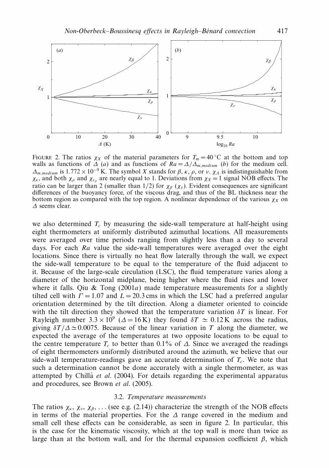
Figure 2. The ratios χX of the material parameters for Tm = 40 ◦C at the bottom and topwalls as functions of ∆ (a) and as functions of Ra = ∆/∆m,medium (b) for the medium cell.∆m,medium is 1.772 × 10⁻⁹ K. The symbol X stands for β , κ , ρ, or ν. χΛ is indistinguishable fromχκ , and both χρ and χcp
are nearly equal to 1. Deviations from χX =1 signal NOB effects. Theratio can be larger than 2 (smaller than 1/2) for χβ (χν). Evident consequences are significantdifferences of the buoyancy force, of the viscous drag, and thus of the BL thickness near thebottom region as compared with the top region. A nonlinear dependence of the various χX on∆ seems clear.
we also determined Tc by measuring the side-wall temperature at half-height usingeight thermometers at uniformly distributed azimuthal locations. All measurementswere averaged over time periods ranging from slightly less than a day to severaldays. For each Ra value the side-wall temperatures were averaged over the eightlocations. Since there is virtually no heat flow laterally through the wall, we expectthe side-wall temperature to be equal to the temperature of the fluid adjacent toit. Because of the large-scale circulation (LSC), the fluid temperature varies along adiameter of the horizontal midplane, being higher where the fluid rises and lowerwhere it falls. Qiu & Tong (2001a) made temperature measurements for a slightlytilted cell with Γ = 1.07 and L =20.3 cms in which the LSC had a preferred angularorientation determined by the tilt direction. Along a diameter oriented to coincidewith the tilt direction they showed that the temperature variation δT is linear. ForRayleigh number 3.3 × 10⁹ (∆ = 16 K) they found δT � 0.12 K across the radius,giving δT /∆ � 0.0075. Because of the linear variation in T along the diameter, weexpected the average of the temperatures at two opposite locations to be equal tothe centre temperature Tc to better than 0.1% of ∆. Since we averaged the readingsof eight thermometers uniformly distributed around the azimuth, we believe that ourside-wall temperature-readings gave an accurate determination of Tc. We note thatsuch a determination cannot be done accurately with a single thermometer, as wasattempted by Chilla et al. (2004). For details regarding the experimental apparatusand procedures, see Brown et al. (2005).
3.2. Temperature measurements
The ratios χκ , χν , χβ , . . . (see e.g. (2.14)) characterize the strength of the NOB effectsin terms of the material properties. For the ∆ range covered in the medium andsmall cell these effects can be considerable, as seen in figure 2. In particular, thisis the case for the kinematic viscosity, which at the top wall is more than twice aslarge than at the bottom wall, and for the thermal expansion coefficient β , which
418 G. Ahlers and others
0 10 20 30 40
–0.5
0.0
0.5
1.0
∆ (K)
Rel
ativ
e de
viat
ion
from
mea
n
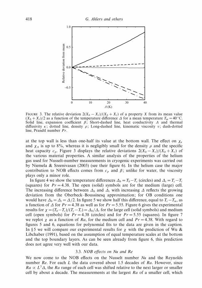
Figure 3. The relative deviation 2(Xb − Xt )/(Xb + Xt ) of a property X from its mean value(Xb + Xt )/2 as a function of the temperature difference ∆ for a mean temperature Tm = 40 ◦C.Solid line, expansion coefficient β; Short-dashed line, heat conductivity Λ and thermaldiffusivity κ; dotted line, density ρ; Long-dashed line, kinematic viscosity ν; dash-dottedline, Prandtl number Pr .
at the top wall is less than one-half its value at the bottom wall. The effect on χκ
and χΛ is up to 8%, whereas it is negligibly small for the density ρ and the specificheat capacity cp . Figure 3 displays the relative deviations 2(Xb − Xt )/(Xb + Xt ) ofthe various material properties. A similar analysis of the properties of the heliumgas used for Nusselt-number measurements in cryogenic experiments was carried outby Niemela & Sreenivasan (2003) (see their figure 6). In the helium case the majorcontribution to NOB effects comes from cp and β; unlike for water, the viscosityplays only a minor role.
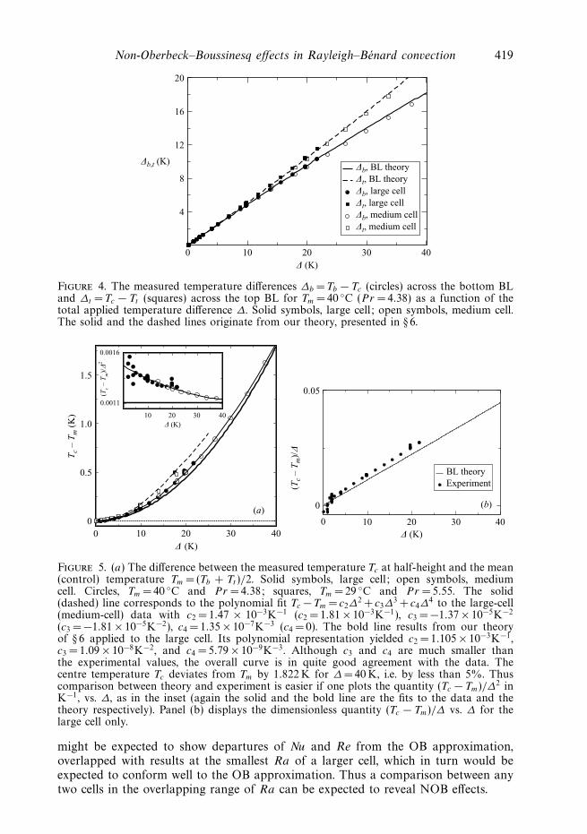
In figure 4 we show the temperature differences ∆b = Tb−Tc (circles) and ∆t = Tc−Tt
(squares) for Pr =4.38. The open (solid) symbols are for the medium (large) cell.The increasing difference between ∆b and ∆t with increasing ∆ reflects the growingdeviation from the Oberbeck–Boussinesq approximation; for OB conditions onewould have ∆b = ∆t =∆/2. In figure 5 we show half this difference, equal to Tc −Tm, asa function of ∆ for Pr = 4.38 as well as for Pr = 5.55. Figure 6 gives the experimentalresults for χ = (Tb−Tc)/(Tc−Tt ) = ∆b/∆t for the large cell (solid symbols) and mediumcell (open symbols) for Pr = 4.38 (circles) and for Pr = 5.55 (squares). In figure 7we replot χ as a function of Ra, for the medium cell and Pr = 4.38. With regard tofigures 5 and 6, equations for polynomial fits to the data are given in the caption.In § 5 we will compare our experimental results for χ with the prediction of Wu &Libchaber (1991), based on the assumption of equal temperature scales at the bottomand the top boundary layers. As can be seen already from figure 6, this predictiondoes not agree very well with our data.
3.3. NOB effects on Nu and Re
We now come to the NOB effects on the Nusselt number Nu and the Reynoldsnumber Re. For each L the data covered about 1.5 decades of Ra. However, sinceRa ∝ L3∆, the Ra range of each cell was shifted relative to the next larger or smallercell by about a decade. The measurements at the largest Ra of a smaller cell, which
Non-Oberbeck–Boussinesq effects in Rayleigh–Benard convection 419
0 10 20 30 40∆ (K)
4
8
12
16
20
∆b,t (K)∆b, BL theory∆t, BL theory∆b, large cell∆t, large cell∆b, medium cell∆t, medium cell
Figure 4. The measured temperature differences ∆b = Tb − Tc (circles) across the bottom BLand ∆t = Tc − Tt (squares) across the top BL for Tm = 40 ◦C (Pr =4.38) as a function of thetotal applied temperature difference ∆. Solid symbols, large cell; open symbols, medium cell.The solid and the dashed lines originate from our theory, presented in § 6.
10 20 30 40
(a)(b)
00
0.5
1.0
1.5
∆ (K)
Tc
– T
m (
K) 10 20 30 40
0.0011
0.0016
∆ (K)
(Tc –
Tm)/∆
2
0 10 20 30 40∆ (K)
0
0.05
(Tc
– T
m)/∆
BL theoryExperiment
Figure 5. (a) The difference between the measured temperature Tc at half-height and the mean(control) temperature Tm = (Tb + Tt )/2. Solid symbols, large cell; open symbols, mediumcell. Circles, Tm =40 ◦C and Pr =4.38; squares, Tm = 29 ◦C and Pr = 5.55. The solid(dashed) line corresponds to the polynomial fit Tc − Tm = c2∆
2 + c3∆3 + c4∆
4 to the large-cell(medium-cell) data with c2 = 1.47 × 10⁻³K−1 (c2 = 1.81 × 10⁻³K−1), c3 = −1.37 × 10⁻⁵K−2
(c3 = −1.81 × 10⁻⁵K−2), c4 = 1.35 × 10⁻⁷K−3 (c4 = 0). The bold line results from our theoryof § 6 applied to the large cell. Its polynomial representation yielded c2 = 1.105 × 10⁻³K−1,c3 = 1.09 × 10⁻⁸K−2, and c4 = 5.79 × 10⁻⁹K−3. Although c3 and c4 are much smaller thanthe experimental values, the overall curve is in quite good agreement with the data. Thecentre temperature Tc deviates from Tm by 1.822 K for ∆= 40 K, i.e. by less than 5%. Thuscomparison between theory and experiment is easier if one plots the quantity (Tc − Tm)/∆2 inK−1, vs. ∆, as in the inset (again the solid and the bold line are the fits to the data and thetheory respectively). Panel (b) displays the dimensionless quantity (Tc − Tm)/∆ vs. ∆ for thelarge cell only.
might be expected to show departures of Nu and Re from the OB approximation,overlapped with results at the smallest Ra of a larger cell, which in turn would beexpected to conform well to the OB approximation. Thus a comparison between anytwo cells in the overlapping range of Ra can be expected to reveal NOB effects.
420 G. Ahlers and others
0 10 20 30 40
0.90
1.00
∆ (K)
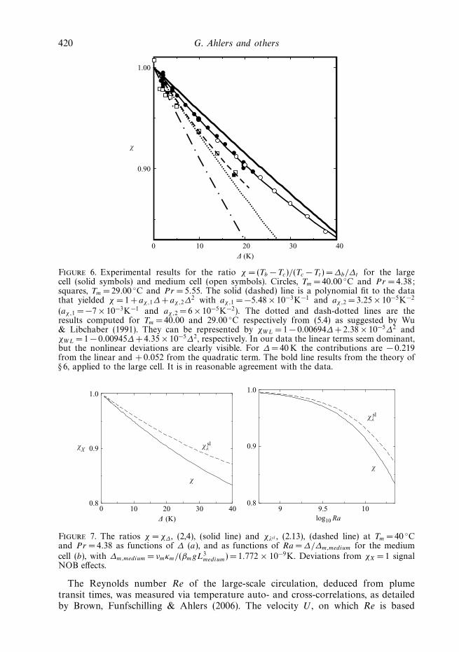
χ
Figure 6. Experimental results for the ratio χ = (Tb − Tc)/(Tc − Tt ) = ∆b/∆t for the largecell (solid symbols) and medium cell (open symbols). Circles, Tm = 40.00 ◦C and Pr = 4.38;squares, Tm = 29.00 ◦C and Pr = 5.55. The solid (dashed) line is a polynomial fit to the datathat yielded χ =1+ aχ,1∆ + aχ,2∆
2 with aχ,1 = −5.48 × 10⁻³K−1 and aχ,2 = 3.25 × 10⁻⁵K−2
(aχ,1 = −7 × 10⁻³K−1 and aχ,2 = 6 × 10⁻⁵K−2). The dotted and dash-dotted lines are theresults computed for Tm = 40.00 and 29.00 ◦C respectively from (5.4) as suggested by Wu& Libchaber (1991). They can be represented by χWL = 1 − 0.00694∆+2.38 × 10⁻⁵∆2 andχWL = 1 − 0.00945∆+4.35 × 10⁻⁵∆2, respectively. In our data the linear terms seem dominant,but the nonlinear deviations are clearly visible. For ∆= 40 K the contributions are − 0.219from the linear and + 0.052 from the quadratic term. The bold line results from the theory of§ 6, applied to the large cell. It is in reasonable agreement with the data.
0 10 20 30 40∆ (K)
0.8
0.9
1.0
χX
χ
χλsl
χλsl
9 9.5 10log10 Ra
0.8
0.9
1.0
χ
Figure 7. The ratios χ = χ∆, (2,4), (solid line) and χλsl , (2.13), (dashed line) at Tm = 40 ◦Cand Pr = 4.38 as functions of ∆ (a), and as functions of Ra = ∆/∆m,medium for the mediumcell (b), with ∆m,medium = νmκm/(βmgL3
medium) = 1.772 × 10⁻⁹K. Deviations from χX = 1 signalNOB effects.
The Reynolds number Re of the large-scale circulation, deduced from plumetransit times, was measured via temperature auto- and cross-correlations, as detailedby Brown, Funfschilling & Ahlers (2006). The velocity U , on which Re is based
Non-Oberbeck–Boussinesq effects in Rayleigh–Benard convection 421
Re—–Ra1/2
0.034
0.036
0.038
2%
109 1010 10110.8
0.9
1.0
Ra
χ
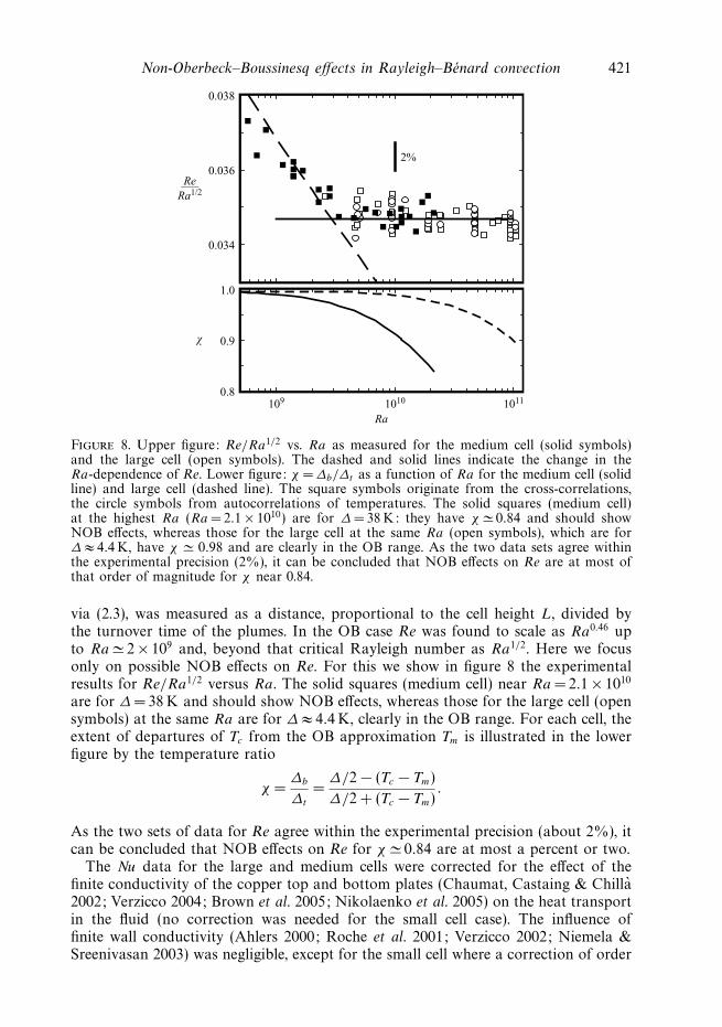
Figure 8. Upper figure: Re/Ra1/2 vs. Ra as measured for the medium cell (solid symbols)and the large cell (open symbols). The dashed and solid lines indicate the change in theRa-dependence of Re. Lower figure: χ = ∆b/∆t as a function of Ra for the medium cell (solidline) and large cell (dashed line). The square symbols originate from the cross-correlations,the circle symbols from autocorrelations of temperatures. The solid squares (medium cell)at the highest Ra (Ra = 2.1 × 10¹⁰) are for ∆= 38 K: they have χ � 0.84 and should showNOB effects, whereas those for the large cell at the same Ra (open symbols), which are for∆ ≈ 4.4 K, have χ � 0.98 and are clearly in the OB range. As the two data sets agree withinthe experimental precision (2%), it can be concluded that NOB effects on Re are at most ofthat order of magnitude for χ near 0.84.
via (2.3), was measured as a distance, proportional to the cell height L, divided bythe turnover time of the plumes. In the OB case Re was found to scale as Ra0.46 upto Ra � 2 × 10⁹ and, beyond that critical Rayleigh number as Ra1/2. Here we focusonly on possible NOB effects on Re. For this we show in figure 8 the experimentalresults for Re/Ra1/2 versus Ra. The solid squares (medium cell) near Ra = 2.1 × 10¹⁰
are for ∆ =38 K and should show NOB effects, whereas those for the large cell (opensymbols) at the same Ra are for ∆ ≈ 4.4 K, clearly in the OB range. For each cell, theextent of departures of Tc from the OB approximation Tm is illustrated in the lowerfigure by the temperature ratio
χ =∆b
∆t
=∆/2 − (Tc − Tm)
∆/2 + (Tc − Tm).
As the two sets of data for Re agree within the experimental precision (about 2%), itcan be concluded that NOB effects on Re for χ � 0.84 are at most a percent or two.
The Nu data for the large and medium cells were corrected for the effect of thefinite conductivity of the copper top and bottom plates (Chaumat, Castaing & Chilla2002; Verzicco 2004; Brown et al. 2005; Nikolaenko et al. 2005) on the heat transportin the fluid (no correction was needed for the small cell case). The influence offinite wall conductivity (Ahlers 2000; Roche et al. 2001; Verzicco 2002; Niemela &Sreenivasan 2003) was negligible, except for the small cell where a correction of order
422 G. Ahlers and others
1% was applied. These experiments are described in detail by Brown et al. (2005).Data for Nu(Ra) under strictly Boussinesq conditions were reported by Funfschillinget al. (2005). Here we concentrate on the results relevant to deviations from the OBapproximation.
One may wonder whether the weak deviation of the aspect ratio from 1 (Γ =0.982,1.002, 0.967 for the large, medium, and small cell, respectively) may affect our resultsfor the Nusselt number, since Shraiman & Siggia (1990) suggested a relatively strongaspect-ratio dependence, Nu ∼ Γ −3/7. However, we note that the actual dependenceis much weaker, as demonstrated experimentally by the work of Funfschilling et al.(2005). There it is shown for instance that the Γ = 6 results for Nu are only about4% below the Γ =1 results. An extremely small Γ -dependence was confirmed morerecently by Sun et al. (2005). It cannot influence the present data over the range0.967 � Γ � 1.002 by a measurable amount. Note also that the experimental analysisof the Γ -dependence included many Γ -values close to Γ = 1, where one would onlyexpect a deformation of the large-scale convection roll, but no extra roll. For example,Nikolaenko et al. (2005) analysed Γ = 0.98, 0.67, 0.43, and 0.275, Funfschilling et al.(2005) analysed Γ =0.967, 0.982, 1.003, 1.506, 2.006, 3.010, and 6.020, and Sun et al.(2005) analysed Γ = 0.67, 1.0, 2.0, 5.0, 10, and 20, all only finding minute dependences.However, we have corrected for tiny systematic errors in the data as discussed alreadyby Funfschilling et al. (2005) (due primarily to errors in the geometry), which canbe different for different cells, by a fraction of a percent by overlapping the Nusseltnumbers (through tiny shifts) of the small and the medium cell and then of themedium and the large cell in their respective OB regimes.
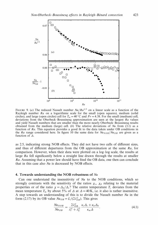
In figure 9(a) we show the results for Nu in the reduced form Nu/Ra1/3 as a functionof Ra (on a logarithmic scale). For the small and medium cell, one sees that Nu inthe NOB region is slightly smaller, but only by a percent or so, than the data in thestrictly Boussinesq range.
In order to show the NOB effect more clearly, we fitted the strictly Oberbeck–Boussinesq data (Funfschilling et al. 2005) to the empirical function
Nu/Ra0.3 =
4∑i=0
bi[log10(Ra)]i (3.1)
and obtained the coefficients b0 = −1.7934, b1 = 0.85734, b2 = −0.13992, b3 =0.009902, b4 = 0.0002490. The function fits the data within their scatter, but shouldnot be relied upon for Ra values outside the range 108 <Ra < 1011 used in the fit.Relative deviations from the function are shown in figure 9(b). There the deviationsfrom the OB approximation become more clear. In figure 10 the same data forNuNOB/NuOB are given as a function of ∆.
Comparison with figures 6 and 7 shows that NOB effects on Nu are negligible inthe range where χ >∼ 0.94 but detectable in the experiment with smaller values of χ ,i.e., with larger NOB deviations from χ = 1. But even when χ reaches its smallestexperimental value, near 0.83, the data fall less than 1.5% below the Boussinesqresults. Even though the NOB effects on Nu are quite small, it is interesting to notethat they diminish the heat transport.
Measurements of χ and of Nu under NOB conditions were made previously byWu & Libchaber (1991) using 4He gas at low temperatures near its critical point. Forsmall Ra, where their cells conformed to the Oberbeck–Boussinesq approximation,they found χ � 1.1. It is not known why their results in this OB limit differedsystematically from unity. At large Ra, however, their results for χ became as large
Non-Oberbeck–Boussinesq effects in Rayleigh–Benard convection 423
0.06
0.07
Ra
Nu—— Ra1/3
108 109 1010 1011
–0.01
0.00
NuOB
(a)
(b)
– 1Nu
Figure 9. (a) The reduced Nusselt number Nu/Ra1/3 on a linear scale as a function of theRayleigh number Ra on a logarithmic scale for the small (open squares), medium (solidcircles), and large (open circles) cell for Tm = 40 ◦C and Pr = 4.38. For the small (medium) cell,deviations from the Oberbeck–Boussinesq approximation are seen at the largest Ra valuesand yield Nusselt numbers that are smaller than the more nearly Oberbeck–Boussinesq resultsobtained from the medium (large) cell. (b) The relative deviations of Nu from (3.1) as afunction of Ra. This equation provides a good fit to the data taken under OB conditions inthe Ra range considered here. In figure 10 the same data for NuNOB/NuOB are given as afunction of ∆.
as 2.5, indicating strong NOB effects. They did not have two cells of different sizes,and thus of different departures from the OB approximation at the same Ra, forcomparison. However, when their data were plotted on a log–log scale, the results atlarge Ra fell significantly below a straight line drawn through the results at smallerRa. Assuming that a power law should have fited the OB data, one then can concludethat in this case also Nu is decreased by NOB effects.
4. Towards understanding the NOB robustness of Nu
Can one understand the insensitivity of Nu to the NOB conditions, which sostrongly contrasts with the sensitivity of the ratios χν , χβ relating to the materialproperties or of the ratio χ = ∆b/∆t? The centre temperature Tc deviates from themean temperature Tm by about 5% of ∆ at ∆ =40 K, i.e. it also is rather insensitive.A step towards an understanding of this is to divide the Nusselt number Nu in theform (2.17) by its OB value NuOB = L/(2λsl
OB). This gives
NuNOB
NuOB
=2λsl
OB
λslt + λsl
b
κt∆t + κb∆b
κm∆. (4.1)
424 G. Ahlers and others
0 10 20 30 40
0.99
1.00
∆ (K)
F1
F2
and
F1
0 20 40 600.98
0.99
1.00
F2
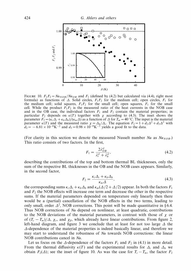
Figure 10. F1F2 = NuNOB/NuOB and F1 (defined by (4.2) but calculated via (4.4), right mostformula) as functions of ∆. Solid circles, F1F2 for the medium cell; open circles, F1 forthe medium cell; solid squares, F1F2 for the small cell; open squares, F1 for the smallcell. While the product F1F2 is the measured ratio of the heat currents in the NOB caseand in the OB case, the individual factors F1 and F2 contain the material properties; inparticular F2 depends on κ(T ) together with χ according to (4.3). The inset shows theparameter F2 = (κt∆t + κb∆b)/(κm∆) as a function of ∆ for Tm = 40 ◦C. The input is the materialparameter κ(T ) and the measured ratio χ = ∆b/∆t . The equation F2 = 1 + d2∆
2 + d3∆3 with
d2 = − 6.81 × 10⁻⁶K−2 and d3 = 0.98 × 10⁻⁸K−3 yields a good fit to the data.
(For clarity in this section we denote the measured Nusselt number Nu as NuNOB .)This ratio consists of two factors. In the first,
F1 =2λsl
OB
λslt + λsl
b
, (4.2)
describing the contributions of the top and bottom thermal BL thicknesses, only thesum of the respective BL thicknesses in the OB and the NOB cases appears. Similarly,in the second factor,
F2 =κt∆t + κb∆b
κm∆, (4.3)
the corresponding sums κt∆t + κb∆b and κm(∆/2 + ∆/2) appear. In both the factors F1
and F2 the NOB effects will increase one term and decrease the other in the respectivesums. If the material parameters depended on temperature only linearly then therewould be a (partial) cancellation of the NOB effects in the two terms, leading toonly small, order ∆2, NOB corrections. This point will be made quantitative in § 6.4.Thus NOB corrections of Nu depend on nonlinear, at least quadratic, contributionsto the NOB deviations of the material parameters, in contrast with those of χ orof (Tc − Tm)/∆, χν , and χβ , which already have linear contributions. From figure 2,left-hand diagram, and figure 3 we conclude that at least for not too large ∆ the∆-dependence of the material properties is indeed basically linear, and therefore wemay start to understand the robustness of Nu towards NOB corrections: the linearNOB contributions cancel in Nu.
Let us focus on the ∆-dependence of the factors F1 and F2 in (4.1) in more detail.From the thermal diffusivity κ(T ) and the experimental results for ∆t and ∆b weobtain F2(∆); see the inset of figure 10. As was the case for Tc − Tm, the factor F2
Non-Oberbeck–Boussinesq effects in Rayleigh–Benard convection 425
can be well represented by the quadratic equation F2 − 1 = d2∆2, without any linear
term (plus of course higher powers of ∆). A least-squares fit to the data yieldedd2 = −6.81 × 10⁻⁶ K−2. We will be able to theoretically understand this quadraticdependence in § 6.4.
With this F2 and using the experimental results for NuNOB/NuOB from figure 10 wecan calculate
F1 =2λsl
OB
λslt + λsl
b
=NuNOB/NuOB
F2
=Q/QOB
F2
, (4.4)
the ratio of the total thermal BL thicknesses. F1 is displayed as open symbols infigure 10. We see that within an experimental uncertainty of 0.2% the BL thicknessratio F1 is independent of ∆, namely F1 ≈ 1. The experimental data thus suggest thatλsl
t + λslb
∼=2λslOB even under strong NOB conditions, where λsl
t /λslb differs considerably
from unity. Because of our finding for thermal convection in water, that the sum ofthe thermal-slope BL thicknesses is conserved within experimental precision,
λslt + λsl
b∼= 2λsl
OB, (4.5)
the NOB corrections on Nu are governed only by F2 and thus are quadratic in ∆ toan extremely good approximation. Finding F2 < 1 would then explain the observedreduction in NuNOB as compared with NuOB .
Figure 10 also shows NuNOB/NuOB = F1F2 for the medium and small cell as solidcircles and open squares, respectively. One sees that within 0.1% or so the datacollapse onto a single curve.
We may speculate on the meaning of these results and cautiously draw some verypreliminary conclusions. Consider a hypothetical case where κ (thus Λ) does notdepend on T i.e. κb = κt = κm, while ν and β vary strongly. Then F2 = 1 for anydistribution of the temperature drops between the top and bottom BLs. Since forconstant κ there is no additional curvature, the temperature profile will not lose itslinear form in the BLs under NOB effects. Nevertheless, λsl
b can still be different fromλsl
t , resulting in Tc �= Tm. As long as the sum of the new BL thicknesses is the same asit was before, i.e. under OB conditions, F1 = 1. This immediately gives QNOB = QOB
or NuNOB = NuOB , i.e. the heat flow will not change despite the fact that Tc �= Tm. Theshift in the bulk temperature from Tm to Tc is the sole effect of the strong variationsin ν and β , but Nu need not see this if κ is T -independent.
If, however, κ depends on T there is additional profile curvature then, which willlead to a change in the heat flow Q. It seems as though F2 is responsible for thisand that we still have F1
∼= 1. Therefore the non-Oberbeck–Boussinesq heat currentQ can be calculated solely from the material properties and the temperature drops∆b and ∆t ,
QNOB
QOB
=NuNOB
NuOB
∼=κb∆b + κt∆t
κm∆. (4.6)
This guarantees the robustness against NOB effects, because the linear term in thenumerator is κm∆ and the cubic terms lead to corrections of order ∆2 for the Q-ratio.
In the case of a curved profile the supposed condition F1∼= 1 could mean that the
value of Tc has to adjust itself in such a way that the sum of the BL thicknessesis invariant, i.e. that (4.5) holds. The volume of the turbulent bulk then is invariantunder deviations from OB conditions; only its time-averaged temperature Tc respondsto the NOB conditions and deviates from Tm. Certainly one has to check in furtherexperiments (or using theoretical arguments) whether the constraint λsl
b + λslt
∼= 2λslOB
holds for liquids other than water in order to validate our finding. We do not know a
426 G. Ahlers and others
physical reason why this should be the case in general; it may be incidental for waterin the temperature range under investigation.
For a more thorough understanding of the robustness of Nu and also Re againstNOB corrections, more theoretical insight into the mechanism of the heat transportis required. Therefore we next consider RB convection models. We shall start with thefirst attempt to explain NOB effects, namely the model of Wu & Libchaber (1991). Itwill turn out that their basic assumption is not consistent with the new data. We then,in § 6, extend the Prandtl–Blasius boundary-layer theory to T -dependent materialparameters. It turns out that this can explain the experimental observations ratherwell.
5. Wu–Libchaber model for NOB effectsWu & Libchaber (1991) and later Zhang et al. (1997) studied the influence of
deviations from OB conditions, both experimentally and also by developing a modelto cope with NOB effects on the Nusselt number. Their model extends the ideasof the Chicago scaling model for RB convection (Castaing et al. 1989) by allowingfor different temperature drops ∆b and ∆t at the bottom and top. We shall brieflysummarize the Wu–Libchaber (WL) results as far as is relevant here, in our notation.
Wu & Libchaber also used (2.5), ∆b + ∆t =∆. Different top and bottom temp-eratures imply different thermal boundary-layer thicknesses, which they introducedby employing heat flux conservation,
Q = Λb
∆b
λb
= Λt
∆t
λt
. (5.1)
These BL thicknesses λb,t are defined in terms of the material properties, taken at themean temperatures Tb and Tt in the respective BLs. These temperatures are
Tb = Tc +∆b
2=
Tc + Tb
2and Tt = Tc − ∆t
2=
Tc + Tt
2.
Next, temperature scales θb and θt are introduced, characterizing the boundarylayers in a different way than by the temperature drops ∆b and ∆t :
θb =νbκb
gβbλ3b
, θt =νtκt
gβtλ3t
. (5.2)
From their data (and later from the model of Zhang et al. 1997) they concludedthat these temperature scales should coincide†, and that, moreover, in the frameworkof the model these scales should be identified with the scale ∆c of the temperaturefluctuations in the bulk,
θb = θt = ∆c. (5.3)
These equalities say that the BL thicknesses respond to the different temperaturedrops at the bottom and top in such a way that the thermal scales communicate
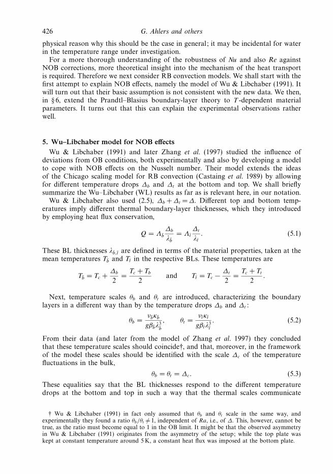
† Wu & Libchaber (1991) in fact only assumed that θb and θt scale in the same way, andexperimentally they found a ratio θb/θt �= 1, independent of Ra, i.e., of ∆. This, however, cannot betrue, as the ratio must become equal to 1 in the OB limit. It might be that the observed asymmetryin Wu & Libchaber (1991) originates from the asymmetry of the setup; while the top plate waskept at constant temperature around 5K, a constant heat flux was imposed at the bottom plate.
Non-Oberbeck–Boussinesq effects in Rayleigh–Benard convection 427
0 10 20 30 40∆ (K)
0.8
0.9
1.0
1.1
χX
χu
χRa
χρ
χu~
9 9.5 10log10 Ra
0.8
0.9
1.0
1.1
χuχRa
χθ
χu~
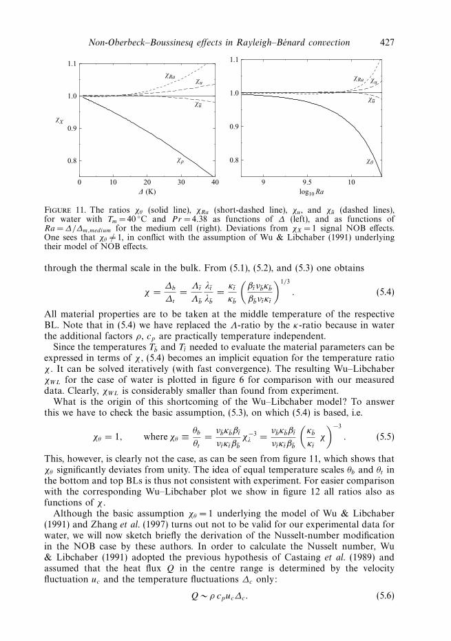
Figure 11. The ratios χθ (solid line), χRa (short-dashed line), χu, and χu (dashed lines),for water with Tm = 40 ◦C and Pr = 4.38 as functions of ∆ (left), and as functions ofRa = ∆/∆m,medium for the medium cell (right). Deviations from χX = 1 signal NOB effects.One sees that χθ �= 1, in conflict with the assumption of Wu & Libchaber (1991) underlyingtheir model of NOB effects.
through the thermal scale in the bulk. From (5.1), (5.2), and (5.3) one obtains
χ =∆b
∆t
=Λt
Λb
λt
λb
=κt
κb
(βtνbκb
βbνtκt
)1/3
. (5.4)
All material properties are to be taken at the middle temperature of the respectiveBL. Note that in (5.4) we have replaced the Λ-ratio by the κ-ratio because in waterthe additional factors ρ, cp are practically temperature independent.
Since the temperatures Tb and Tt needed to evaluate the material parameters can beexpressed in terms of χ , (5.4) becomes an implicit equation for the temperature ratioχ . It can be solved iteratively (with fast convergence). The resulting Wu–LibchaberχWL for the case of water is plotted in figure 6 for comparison with our measureddata. Clearly, χWL is considerably smaller than found from experiment.
What is the origin of this shortcoming of the Wu–Libchaber model? To answerthis we have to check the basic assumption, (5.3), on which (5.4) is based, i.e.
χθ = 1, whereχθ ≡ θb
θt
=νbκbβt
νtκtβb
χ−3λ =
νbκbβt
νtκtβb
(κb
κt
χ
)−3
. (5.5)
This, however, is clearly not the case, as can be seen from figure 11, which shows thatχθ significantly deviates from unity. The idea of equal temperature scales θb and θt inthe bottom and top BLs is thus not consistent with experiment. For easier comparisonwith the corresponding Wu–Libchaber plot we show in figure 12 all ratios also asfunctions of χ .
Although the basic assumption χθ = 1 underlying the model of Wu & Libchaber(1991) and Zhang et al. (1997) turns out not to be valid for our experimental data forwater, we will now sketch briefly the derivation of the Nusselt-number modificationin the NOB case by these authors. In order to calculate the Nusselt number, Wu& Libchaber (1991) adopted the previous hypothesis of Castaing et al. (1989) andassumed that the heat flux Q in the centre range is determined by the velocityfluctuation uc and the temperature fluctuations ∆c only:
Q ∼ ρ cpuc∆c. (5.6)
428 G. Ahlers and others
0.80 0.85 0.90 0.95 1.00χ = χ
∆
0.7
0.8
0.9
1.0
1.1
χX
χu
χRa
χθ
χu~
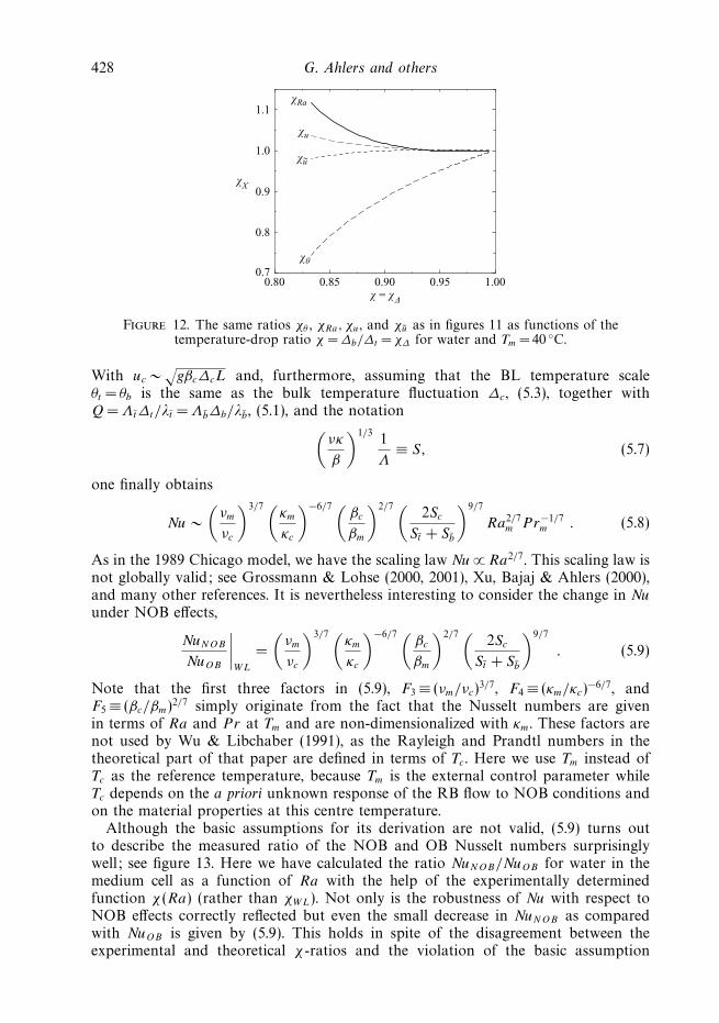
Figure 12. The same ratios χθ , χRa, χu, and χu as in figures 11 as functions of thetemperature-drop ratio χ = ∆b/∆t =χ∆ for water and Tm = 40 ◦C.
With uc ∼√
gβc∆cL and, furthermore, assuming that the BL temperature scaleθt = θb is the same as the bulk temperature fluctuation ∆c, (5.3), together withQ =Λt∆t/λt = Λb∆b/λb, (5.1), and the notation(
νκ
β
)1/31
Λ≡ S, (5.7)
one finally obtains
Nu ∼(
νm
νc
)3/7 (κm
κc
)−6/7 (βc
βm
)2/7 (2Sc
St + Sb
)9/7
Ra2/7m P r−1/7
m . (5.8)
As in the 1989 Chicago model, we have the scaling law Nu ∝ Ra2/7. This scaling law isnot globally valid; see Grossmann & Lohse (2000, 2001), Xu, Bajaj & Ahlers (2000),and many other references. It is nevertheless interesting to consider the change in Nu
under NOB effects,
NuNOB
NuOB
∣∣∣∣WL
=
(νm
νc
)3/7 (κm
κc
)−6/7 (βc
βm
)2/7 (2Sc
St + Sb
)9/7
. (5.9)
Note that the first three factors in (5.9), F3 ≡ (νm/νc)3/7, F4 ≡ (κm/κc)
−6/7, andF5 ≡ (βc/βm)2/7 simply originate from the fact that the Nusselt numbers are givenin terms of Ra and Pr at Tm and are non-dimensionalized with κm. These factors arenot used by Wu & Libchaber (1991), as the Rayleigh and Prandtl numbers in thetheoretical part of that paper are defined in terms of Tc. Here we use Tm instead ofTc as the reference temperature, because Tm is the external control parameter whileTc depends on the a priori unknown response of the RB flow to NOB conditions andon the material properties at this centre temperature.
Although the basic assumptions for its derivation are not valid, (5.9) turns outto describe the measured ratio of the NOB and OB Nusselt numbers surprisinglywell; see figure 13. Here we have calculated the ratio NuNOB/NuOB for water in themedium cell as a function of Ra with the help of the experimentally determinedfunction χ(Ra) (rather than χWL). Not only is the robustness of Nu with respect toNOB effects correctly reflected but even the small decrease in NuNOB as comparedwith NuOB is given by (5.9). This holds in spite of the disagreement between theexperimental and theoretical χ-ratios and the violation of the basic assumption
Non-Oberbeck–Boussinesq effects in Rayleigh–Benard convection 429
9 9.5 10log10 Ra
0.97
0.98
0.99
1.00
1.01
1.02
1.03
NuNOB———NuOB
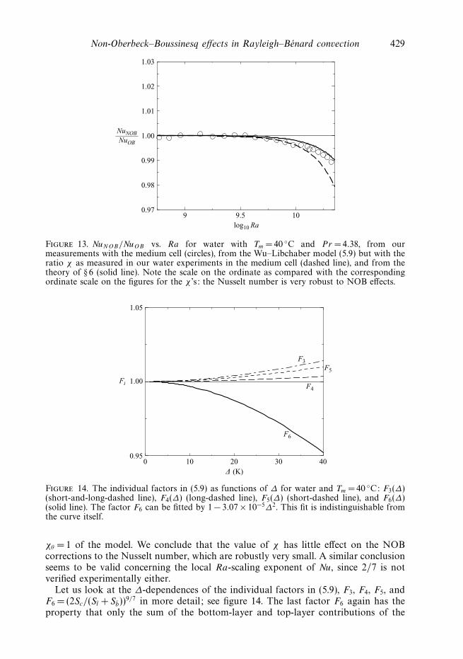
Figure 13. NuNOB/NuOB vs. Ra for water with Tm = 40 ◦C and Pr = 4.38, from ourmeasurements with the medium cell (circles), from the Wu–Libchaber model (5.9) but with theratio χ as measured in our water experiments in the medium cell (dashed line), and from thetheory of § 6 (solid line). Note the scale on the ordinate as compared with the correspondingordinate scale on the figures for the χ ’s: the Nusselt number is very robust to NOB effects.
0 10 20 30 40∆ (K)
0.95
1.00
1.05
Fi
F3
F4
F5
F6
Figure 14. The individual factors in (5.9) as functions of ∆ for water and Tm = 40 ◦C: F3(∆)(short-and-long-dashed line), F4(∆) (long-dashed line), F5(∆) (short-dashed line), and F6(∆)(solid line). The factor F6 can be fitted by 1 − 3.07 × 10⁻⁵∆2. This fit is indistinguishable fromthe curve itself.
χθ = 1 of the model. We conclude that the value of χ has little effect on the NOBcorrections to the Nusselt number, which are robustly very small. A similar conclusionseems to be valid concerning the local Ra-scaling exponent of Nu, since 2/7 is notverified experimentally either.
Let us look at the ∆-dependences of the individual factors in (5.9), F3, F4, F5, andF6 = (2Sc/(St + Sb))
9/7 in more detail; see figure 14. The last factor F6 again has theproperty that only the sum of the bottom-layer and top-layer contributions of the

430 G. Ahlers and others
quantity S appears. Thus, in the lowest, linear, order in the temperature deviationshere also the NOB effects from the top and bottom BLs compensate each other.Indeed, the factor F6 is nicely described by a quadratic dependence on ∆, namely byF6 = 1 − 3.07 × 10⁻⁵∆2. The other factors Fi , i = 3, 4, 5, introduce linear dependenceson ∆, however.
Since the ratios of the bottom and top quantities are of particular interest incharacterizing deviations from OB conditions quantitatively, χ = χ∆ in particular butalso χκ, χν, χβ (and, in the framework of the Wu–Libchaber model, χθ ), we now checkother such ratios. Consider first the ∆ or ∆/∆m,medium = Ra dependence of the ratioof the bottom and top Rayleigh numbers χRa = Rab/Rat , with
Rab =gβbλ
3b∆b
νbκb
=∆b
θb
(5.10)
and Rat defined correspondingly. We have
χRa =Rab
Rat
= χχ−1θ . (5.11)
The BL thickness ratio in the Wu–Libchaber approximation is χλ = λb/λt = (κb/κt ) χ.
Furthermore, there are various velocity scales in the RB system. Define wb as thatvelocity scale in the BL for which buoyancy is of the order of the viscous loss,gβb∆b ∼ νbwb/λ
2b, leading to
χw =wb
wt
=βbνt
βtνb
∆b
∆t
(λb
λt
)2
= χβχ−1ν χχ2
λ. (5.12)
Also of interest is this velocity scale in the boundary layers. In the bottom BL therelevant length scale is λb and the relevant temperature difference is either ∆b or θb.Defining
ub = (βbg∆bλb)1/2 and ub = (βbgθbλb)
1/2 =
(νb
λb
κb
λb
)1/2
one is led to
χu =ub
ut
=
(βb
βt
χχλ
)1/2
(5.13)
and
χu =ub
ut
= χ1/2ν χ1/2
κ χ−1λ . (5.14)
Note that ub (and correspondingly ut ) is the geometric mean of the viscous andthermal molecular velocities in the boundary layer, independently of any buoyancy.
We present various of these ratios for the case of water as working fluid in figure 11,as functions of ∆ and of ∆/∆m,medium = Ra. They all show prominent NOB effects. TheRa-ratios χRa and also χu have only moderate deviations from the OB value χX =1.But apparently they too are not ∆-independent constants. For better comparison withthe curves of Wu and Libchaber (Wu & Libchaber 1991) we also present the ratiosof interest as functions of the preferred measure for NOB effects, the BL temperatureratio χ = χ∆ (figure 12).
Non-Oberbeck–Boussinesq effects in Rayleigh–Benard convection 431
6. Extension of boundary-layer theory to NOB conditions6.1. Motivation
The previous section showed the shortcomings of the Wu–Libchaber model in explain-ing the centre temperature Tc, and thus χ , in the examined NOB case of water. In thissection we will present an alternative theory which will not have these shortcomingsand which will be able to account consistently for all measured NOB effects in relationto the OB data for water. It is based on the Prandtl–Blasius theory for laminar BLs(Prandtl 1905; Blasius 1908; Pohlhausen 1921; Meksyn 1961; Landau & Lifshitz1987; Schlichting & Gersten 2000), extended to the case of temperature-dependentviscosity and thermal diffusivity (Plapp 1957); see also Zhang et al. (1997) and Wall &Wilson (1997) who considered the case of temperature-dependent viscosity only. Thejustification for starting from the Prandtl–Blasius BL theory is that, for water, evenfor Ra = 1011 the wall Reynolds number is not larger than about 100. Indeed, theGrossmann–Lohse unifying theory of RB convection (Grossmann & Lohse 2000, 2001,2002, 2004), which is able to account for the measured Nu(Ra, P r) and Re(Ra, P r)in a considerable part of parameter space, employs the scaling of the Prandtl–BlasiusBL theory as a central ingredient although the layers certainly show plume separationand therefore time dependence. But they are not yet fully turbulent and therefore notfluctuation dominated.
In § 2.4 we have already addressed how the BL thicknesses will be modified in theNOB case. We will now calculate the full velocity and temperature profiles and fromthose derive the centre temperature Tc and thus the ratio χ = ∆b/∆t (§ 6.2), which arefound to be in very good agreement with the experimental data. No fitting parameterhas to be introduced. In addition we employ the experimental finding of figure 10that for water the factor F1 = 1 within the experimental resolution in the ∆ range ofinterest, meaning that the sum of the top and bottom thermal-boundary-layer widths(based on the slopes of the temperature profiles at the plates) remains unchanged inthe NOB case. Then the theory also gives the measured small reduction of Nusseltnumber for the NOB case and an at most 0.5% increase in the Reynolds number forthe ∆ considered here; this is also consistent with the experimental data (§ 6.3). In§ 6.4 we explore the origin of the NOB corrections by studying hypothetical liquidsfor which only one of the material parameters is temperature dependent. In § 6.5 weapply our theory to glycerol and make predictions for the NOB effects in that liquid.
6.2. Viscous and thermal boundary layers with temperature-dependent viscosity andthermal diffusivity
As pointed out in § 2, for water one can assume to a very good approximation thatthe fluid density and the isobaric specific heat capacity are constant, i.e. throughoutthe liquid they are equal to ρm and cp,m, respectively. In contrast, the temperaturedependences of the kinematic viscosity ν(T ) = η(T )/ρm and the thermal diffusivityκ(T ) = Λ(T )/(cp,mρm) are explicitly taken into consideration and calculated accordingto the Appendix.
In this approximation Prandtl’s equation, on which Prandtl’s stationary-BL theoryis based, reads
ux∂xux + uz∂zux = ∂z(ν∂zux). (6.1)
Pressure contributions are omitted. ux is the horizontal velocity component at thebottom or top plates in the direction of the large-scale circulation (the wind ofturbulence) and uz is the vertical velocity component. Both velocity components aretaken to be uniform in the lateral, y-direction, i.e. in the direction perpendicular to the
432 G. Ahlers and others
wind, and are functions of x and z only. The following boundary conditions apply:
ux(x, 0) = 0, (6.2)
uz(x, 0) = 0, (6.3)
ux(x, ∞) = UNOB. (6.4)
The longitudinal asymptotic velocity UNOB outside the viscous BL is identified withthe wind of turbulence. Note that UNOB is not necessarily the same as UOB , since itmay vary with the bulk properties, in particular with Tc and thus with ∆. Its value ispart of the boundary conditions. For solving the BL equations the only thing whichmatters is to fix the asymptotic (z → ∞) value of ux(x, z). The difference between UNOB
and UOB will be determined by an additional input, taken from an argument beyondboundary-layer theory, namely, the experimental finding that the sum of the physicalboundary-layer thicknesses for water has been measured as independent of ∆.
Analogously, the thermal boundary layer is described by
ux∂xT + uz∂zT = ∂z
(κ ∂zT
), (6.5)
with boundary conditions
T (x, 0) = Tb or T (x, 0) = Tt , (6.6)
T (x, ∞) = Tc. (6.7)
The two possible boundary conditions describe two plates facing each other, one thetop plate and the other the bottom plate. The asymptotic temperature of the fluidoutside each thermal BL is Tc, which under NOB conditions is not the same as Tm. Itsvalue is part of the boundary conditions as well and is determined by the constraintthat the thermal current across the RB container is conserved, as will be explainedbelow.
Now, the temperature is measured as the deviation from the top temperature andis non-dimensionalized using ∆:
Θ =T − Tt
∆=
T − Tm
∆+
1
2. (6.8)
(Distinguish Θ from θ , the temperature in K as measured from the chosen referencetemperature, usually Tm, introduced already above.) Then Θm = 1/2 and the thermalboundary conditions for the bottom and top plates read Θb = 1 and Θt = 0. Thecentral new element as compared with the standard laminar BL theory is that boththe kinematic viscosity and the thermal diffusivity are now temperature dependent; indimensionless form we have ν(Θ) = ν(T )/νm and κ(Θ) = κ(T )/κm, respectively, givingrise to extra terms when the z-derivatives on the right-hand sides of (6.1) and (6.5)are performed.
We now reduce (6.1) and (6.5) to ODEs by introducing a streamfunction ψ andthen employing its self-similarity under x and z changes. The streamfunction ψ canbe introduced because Prandtl’s BL theory deals with two-dimensional incompressibleflow. It satisfies ux = ∂zψ and uz = −∂xψ . In analogy with the OB case, we introducethe transverse length scale �NOB:
�NOB ≡√
x νm
UNOB
. (6.9)
This length scale is defined in terms of the asymptotic velocity UNOB as the velocityscale, since this choice guarantees that the boundary condition for the stream-function
Non-Oberbeck–Boussinesq effects in Rayleigh–Benard convection 433
will always be Ψ ′(∞) = 1, independently of the value of ∆. As UNOB is a prioriunknown, so is �NOB . Next the similarity variable ξ is introduced:
ξ = z
√UNOB
x νm
=z
�NOB
. (6.10)
The streamfunction ψ(x, z) is assumed to depend on this x, z-combinationonly, implying a self-similar solution. As in the standard Prandtl theory, ψ isnon-dimensionalized as
Ψ (ξ ) =ψ(x, z)
�NOBUNOB
. (6.11)
With this non-dimensional self-similarity ansatz for the stream function one findsfrom the Prandtl equation (6.1) the ODE
νΨ ′′′ +
(1
2Ψ +
dν
dΘΘ ′
)Ψ ′′ = 0. (6.12)
The boundary conditions are
Ψ (0) = 0, (6.13)
Ψ ′(0) = 0, (6.14)
Ψ ′(∞) = 1. (6.15)
Note that the velocity profile Ψ ′ = ux/UNOB depends explicitly on viscosity andimplicitly on the thermal diffusivity (since the Θ-profile depends on Pr , as will beshown below; see (6.16)). Therefore, the solution of the dimensionless boundary-valueproblem (6.12)–(6.15) is non-universal. Namely, it depends on the material parametersand their respective temperature dependences.
Correspondingly, from the temperature equation (6.5) one obtains for the similarityfunction Θ describing the temperature field Θ(x, z) =Θ(ξ )
κ Θ ′′ +
(1
2Pr Ψ +
dκ
dΘΘ ′
)Θ ′ = 0. (6.16)
There are two possible boundary conditions, either for the bottom or for the top BL:
Θ(0) = Θb = 1 or Θ(0) = Θt = 0, (6.17)
together with
Θ(∞) = Θc. (6.18)
Thus, in the RB configuration, each thermal plate is associated with a boundarylayer described by (6.12)–(6.15) coupled to (6.16)–(6.18). Therefore, in principle, itwould be just a matter of integrating the top and bottom BL equations, as in theOB case. However, the NOB case has a subtle point: the asymptotic temperatureΘc = (Tc − Tt )/∆, with 0 <Θc < 1, is a response parameter, which has not been fixedyet. Therefore, in order to solve the BL equations one has first to identify the centre(bulk) temperature Tc and thus the boundary condition (6.18).
We determine Θc by the constraint that the thermal flux across the cell is conservedand therefore the influx at the bottom must be the same as the outflux at the top,J (z = 0) = J (z = L). This means that
κb∂zT |b = κt∂zT |t (6.19)
434 G. Ahlers and others
0 2ω
0.5
1.0(a) (b)
Ψ′
3.5
ξ
0
1
ΘBottom BLTop BL
Θc
λbsl~
λtsl~
λb99%~ ~
λt99%1 3 4 5 6 7
NOB bottom BL
NOB top BL
OB bottom and top BL
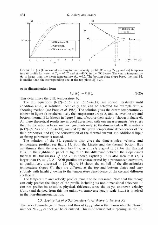
Figure 15. (a) (Dimensionless) longitudinal velocity profile Ψ ′ = ux/UNOB and (b) tempera-ture Θ profile for water at Tm = 40 ◦C and ∆= 40 ◦C in the NOB case. The centre temperatureΘc is larger than the mean temperature Θm = 0.5. The bottom-plate slope-based thermal BLis smaller than the corresponding one at the top plate, λsl
b < λslt .
or in dimensionless form
κb | Θ ′b| = κtΘ
′t . (6.20)
This determines the bulk temperature Θc.The BL equations (6.12)–(6.15) and (6.16)–(6.18) are solved iteratively until
condition (6.20) is satisfied. Technically, this can be achieved for example with ashooting method (see Press et al. 1986). The solution gives the centre temperature Tc
(shown in figure 5), or alternatively the temperature drops ∆t and ∆b over the top andbottom thermal BLs (shown in figure 4) and of course their ratio χ (shown in figure 6).All these theoretical results are in good agreement with our measurements. We stressthat the derivation is based on two ingredients only: (i) the dimensionless BL equations(6.12)–(6.15) and (6.16)–(6.18), assisted by the given temperature dependences of thefluid properties, and (ii) the conservation of the thermal current. No additional inputor fitting parameter is needed.
The solution of the BL equations also gives the dimensionless velocity andtemperature profiles; see figure 15. Both the kinetic and the thermal bottom BLsare thinner than the respective top BLs, as already argued in § 2 for the thermalBLs. In the right-hand panel of figure 15 the difference between the slope-basedthermal BL thicknesses λsl
b and λslt is shown explicitly. It is also seen that Θc is
larger than Θm = 1/2. All NOB profiles are characterized by a pronounced curvature,as qualitatively discussed in § 2. Figure 16 shows the moduli of the dimensionlesstemperature slopes Θ ′; they are different at the top and bottom plates and varystrongly with height z, owing to the temperature dependence of the thermal diffusioncoefficient.
The temperature and velocity profiles remain to be measured. Note that the theorycan only predict the shape of the profile including its non-dimensional thickness; itcan not predict its absolute, physical, thickness, since the as yet unknown velocityUNOB (and derived from this the unknown transverse length scale �NOB) is involvedin the non-dimensionalization.
6.3. Application of NOB boundary-layer theory to Nu and Re
The lack of knowledge of UNOB (and thus of �NOB) also is the reason why the Nusseltnumber NuNOB cannot yet be calculated. This is of course not surprising, as the BL
Non-Oberbeck–Boussinesq effects in Rayleigh–Benard convection 435
1 2 4ξ
0
0.1
0.2
0.3
Θ′
3 5
NOB bottom BL
NOB top BL
OB bottom and top BL
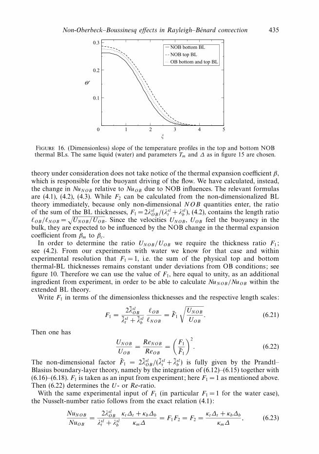
Figure 16. (Dimensionless) slope of the temperature profiles in the top and bottom NOBthermal BLs. The same liquid (water) and parameters Tm and ∆ as in figure 15 are chosen.
theory under consideration does not take notice of the thermal expansion coefficient β ,which is responsible for the buoyant driving of the flow. We have calculated, instead,the change in NuNOB relative to NuOB due to NOB influences. The relevant formulasare (4.1), (4.2), (4.3). While F2 can be calculated from the non-dimensionalized BLtheory immediately, because only non-dimensional NOB quantities enter, the ratioof the sum of the BL thicknesses, F1 = 2λsl
OB/(λslt + λsl
b ), (4.2), contains the length ratio�OB/�NOB =
√UNOB/UOB . Since the velocities UNOB , UOB feel the buoyancy in the
bulk, they are expected to be influenced by the NOB change in the thermal expansioncoefficient from βm to βc.
In order to determine the ratio UNOB/UOB we require the thickness ratio F1;see (4.2). From our experiments with water we know for that case and withinexperimental resolution that F1 = 1, i.e. the sum of the physical top and bottomthermal-BL thicknesses remains constant under deviations from OB conditions; seefigure 10. Therefore we can use the value of F1, here equal to unity, as an additionalingredient from experiment, in order to be able to calculate NuNOB/NuOB within theextended BL theory.
Write F1 in terms of the dimensionless thicknesses and the respective length scales:
F1 =2λsl
OB
λslt + λsl
b
�OB
�NOB
= F1
√UNOB
UOB
. (6.21)
Then one has
UNOB
UOB
=ReNOB
ReOB
=
(F1
F1
)2
. (6.22)
The non-dimensional factor F1 = 2λslOB/(λsl
t + λslb ) is fully given by the Prandtl–
Blasius boundary-layer theory, namely by the integration of (6.12)–(6.15) together with(6.16)–(6.18). F1 is taken as an input from experiment; here F1 = 1 as mentioned above.Then (6.22) determines the U - or Re-ratio.
With the same experimental input of F1 (in particular F1 = 1 for the water case),the Nusselt-number ratio follows from the exact relation (4.1):
NuNOB
NuOB
=2λsl
OB
λslt + λsl
b
κt∆t + κb∆b
κm∆= F1F2 = F2 =
κt∆t + κb∆b
κm∆, (6.23)
436 G. Ahlers and others
0 10 20 30 40∆ (K)
1.00
1.01
ReNOB——–ReOB
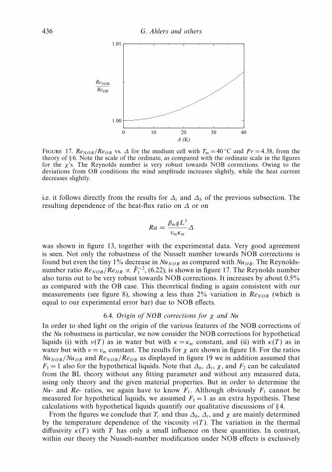
Figure 17. ReNOB/ReOB vs. ∆ for the medium cell with Tm = 40 ◦C and Pr = 4.38, from thetheory of § 6. Note the scale of the ordinate, as compared with the ordinate scale in the figuresfor the χ ’s. The Reynolds number is very robust towards NOB corrections. Owing to thedeviations from OB conditions the wind amplitude increases slightly, while the heat currentdecreases slightly.
i.e. it follows directly from the results for ∆t and ∆b of the previous subsection. Theresulting dependence of the heat-flux ratio on ∆ or on
Ra =βmgL3
νmκm
∆
was shown in figure 13, together with the experimental data. Very good agreementis seen. Not only the robustness of the Nusselt number towards NOB corrections isfound but even the tiny 1% decrease in NuNOB as compared with NuOB . The Reynolds-number ratio ReNOB/ReOB ∝ F −2
1 , (6.22), is shown in figure 17. The Reynolds numberalso turns out to be very robust towards NOB corrections. It increases by about 0.5%as compared with the OB case. This theoretical finding is again consistent with ourmeasurements (see figure 8), showing a less than 2% variation in ReNOB (which isequal to our experimental error bar) due to NOB effects.
6.4. Origin of NOB corrections for χ and Nu
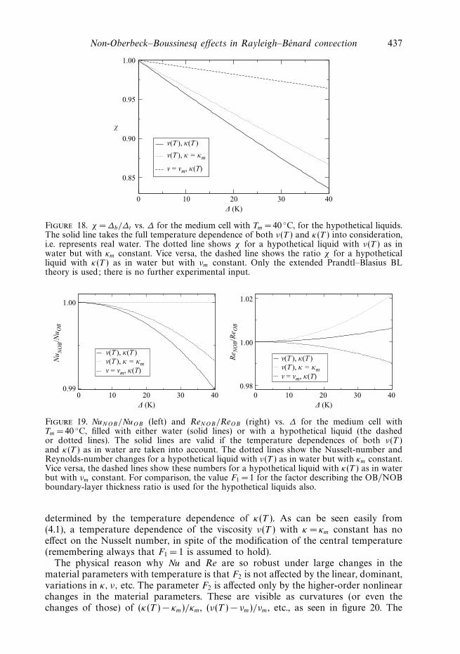
In order to shed light on the origin of the various features of the NOB corrections ofthe Nu robustness in particular, we now consider the NOB corrections for hypotheticalliquids (i) with ν(T ) as in water but with κ = κm constant, and (ii) with κ(T ) as inwater but with ν = νm constant. The results for χ are shown in figure 18. For the ratiosNuNOB/NuOB and ReNOB/ReOB as displayed in figure 19 we in addition assumed thatF1 = 1 also for the hypothetical liquids. Note that ∆b, ∆t , χ , and F2 can be calculatedfrom the BL theory without any fitting parameter and without any measured data,using only theory and the given material properties. But in order to determine theNu- and Re- ratios, we again have to know F1. Although obviously F1 cannot bemeasured for hypothetical liquids, we assumed F1 = 1 as an extra hypothesis. Thesecalculations with hypothetical liquids quantify our qualitative discussions of § 4.
From the figures we conclude that Tc and thus ∆b, ∆t , and χ are mainly determinedby the temperature dependence of the viscosity ν(T ). The variation in the thermaldiffusivity κ(T ) with T has only a small influence on these quantities. In contrast,within our theory the Nusselt-number modification under NOB effects is exclusively
Non-Oberbeck–Boussinesq effects in Rayleigh–Benard convection 437
0 10 20 30 40∆ (K)
0.85
0.90
0.95
1.00
χ
ν = νm, κ(T)
ν(T ), κ(T )
ν(T ), κ = κm
Figure 18. χ = ∆b/∆t vs. ∆ for the medium cell with Tm =40 ◦C, for the hypothetical liquids.The solid line takes the full temperature dependence of both ν(T ) and κ(T ) into consideration,i.e. represents real water. The dotted line shows χ for a hypothetical liquid with ν(T ) as inwater but with κm constant. Vice versa, the dashed line shows the ratio χ for a hypotheticalliquid with κ(T ) as in water but with νm constant. Only the extended Prandtl–Blasius BLtheory is used; there is no further experimental input.
100 20 30 40∆ (K)
100 20 30 40∆ (K)
0.99
1.00
Nu N
OB/N
u OB
0.98
1.00
1.02
Re N
OB/R
e OB
ν = νm, κ(T)
ν(T ), κ(T )ν(T ), κ = κm
ν = νm, κ(T)
ν(T ), κ(T )ν(T ), κ = κm
Figure 19. NuNOB/NuOB (left) and ReNOB/ReOB (right) vs. ∆ for the medium cell withTm = 40 ◦C, filled with either water (solid lines) or with a hypothetical liquid (the dashedor dotted lines). The solid lines are valid if the temperature dependences of both ν(T )and κ(T ) as in water are taken into account. The dotted lines show the Nusselt-number andReynolds-number changes for a hypothetical liquid with ν(T ) as in water but with κm constant.Vice versa, the dashed lines show these numbers for a hypothetical liquid with κ(T ) as in waterbut with νm constant. For comparison, the value F1 = 1 for the factor describing the OB/NOBboundary-layer thickness ratio is used for the hypothetical liquids also.
determined by the temperature dependence of κ(T ). As can be seen easily from(4.1), a temperature dependence of the viscosity ν(T ) with κ = κm constant has noeffect on the Nusselt number, in spite of the modification of the central temperature(remembering always that F1 = 1 is assumed to hold).
The physical reason why Nu and Re are so robust under large changes in thematerial parameters with temperature is that F2 is not affected by the linear, dominant,variations in κ, ν, etc. The parameter F2 is affected only by the higher-order nonlinearchanges in the material parameters. These are visible as curvatures (or even thechanges of those) of (κ(T ) − κm)/κm, (ν(T ) − νm)/νm, etc., as seen in figure 20. The
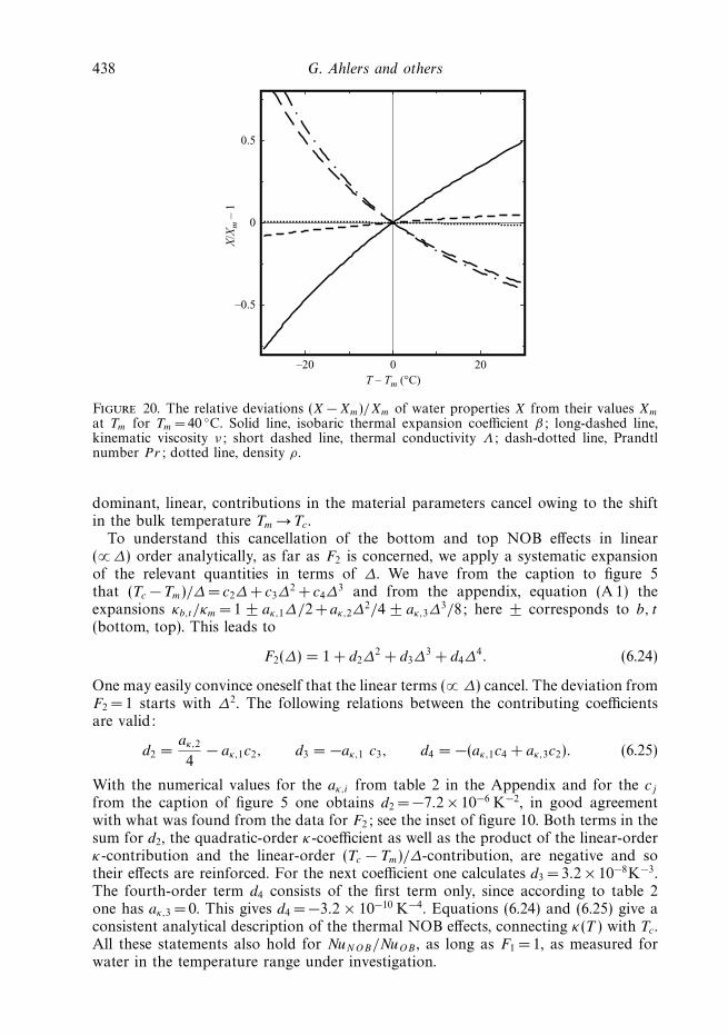
438 G. Ahlers and others
–20 0 20
–0.5
0
0.5
T – Tm (°C)
X/X
m –
1
Figure 20. The relative deviations (X − Xm)/Xm of water properties X from their values Xm
at Tm for Tm = 40 ◦C. Solid line, isobaric thermal expansion coefficient β; long-dashed line,kinematic viscosity ν; short dashed line, thermal conductivity Λ; dash-dotted line, Prandtlnumber Pr; dotted line, density ρ.
dominant, linear, contributions in the material parameters cancel owing to the shiftin the bulk temperature Tm → Tc.
To understand this cancellation of the bottom and top NOB effects in linear(∝ ∆) order analytically, as far as F2 is concerned, we apply a systematic expansionof the relevant quantities in terms of ∆. We have from the caption to figure 5that (Tc − Tm)/∆ = c2∆ + c3∆
2 + c4∆3 and from the appendix, equation (A 1) the
expansions κb,t /κm = 1 ± aκ,1∆/2 + aκ,2∆2/4 ± aκ,3∆
3/8; here ± corresponds to b, t
(bottom, top). This leads to
F2(∆) = 1 + d2∆2 + d3∆
3 + d4∆4. (6.24)
One may easily convince oneself that the linear terms (∝ ∆) cancel. The deviation fromF2 = 1 starts with ∆2. The following relations between the contributing coefficientsare valid:
d2 =aκ,2
4− aκ,1c2, d3 = −aκ,1 c3, d4 = −(aκ,1c4 + aκ,3c2). (6.25)
With the numerical values for the aκ,i from table 2 in the Appendix and for the cj
from the caption of figure 5 one obtains d2 = −7.2 × 10⁻⁶ K−2, in good agreementwith what was found from the data for F2; see the inset of figure 10. Both terms in thesum for d2, the quadratic-order κ-coefficient as well as the product of the linear-orderκ-contribution and the linear-order (Tc − Tm)/∆-contribution, are negative and sotheir effects are reinforced. For the next coefficient one calculates d3 = 3.2 × 10⁻⁸K−3.The fourth-order term d4 consists of the first term only, since according to table 2one has aκ,3 = 0. This gives d4 = −3.2 × 10⁻¹⁰ K−4. Equations (6.24) and (6.25) give aconsistent analytical description of the thermal NOB effects, connecting κ(T ) with Tc.All these statements also hold for NuNOB/NuOB , as long as F1 = 1, as measured forwater in the temperature range under investigation.

Non-Oberbeck–Boussinesq effects in Rayleigh–Benard convection 439
The quadratic dependence of F2 on ∆ is in agreement with experiment (see figure 10)and was discussed in § 4. We may now also understand what sets the sign of theNOB correction to the Nusselt number (provided that F1 = 1): It is the sign of thesum constituting d2 = −aκ,1c2 + aκ,2/4. The factor aκ,1 results from the temperaturedependence of the thermal diffusivity, while the factor c2 in addition strongly dependson the temperature dependence of the viscosity ν(T ); it immediately reflects whether Tc
is larger than Tm (as for water) or smaller. Furthermore, the curvature coefficient aκ,2 ofthe thermal diffusivity κ(T ) contributes to the sign of the deviation Tc −Tm. For waterboth terms in the sum are negative, thus adding to the downshift of NuNOB/NuOB .As emphasized already, the effect is quadratic in ∆; the linear contributions from thetop and the bottom BLs cancel.
The NOB modifications of the Reynolds number Re are more subtle; see the right-hand diagram in figure 19. For water, the NOB effects of a temperature-dependentviscosity with a constant thermal diffusivity (resulting in a slight enhancement of Re)and those of a temperature-dependent thermal diffusivity with a constant viscosity(resulting in a slight decrease of Re) partly compensate each other, leading to only atiny net enhancement of Re. The reason for the enhanced Reynolds number for thecase ν(T ), κ = κm, is the overall temperature increase in the cell, Tc >Tm, resulting ina smaller cell-averaged viscosity. Note again that according to our theory this doesnot have any effect on the Nusselt number. The reason for the reduced Reynoldsnumber for the case κ(T ), ν = νm, is less obvious. Technically, it results from F1 > 1,i.e. 2λsl
OB > λslt + λsl
b . But remember that for this discussion we have always made theassumption that F1 = 1.
6.5. NOB effects in glycerol
We now consider theoretically NOB effects for another liquid besides water, namelyglycerol. The reason is to have an independent test for our theory, as there are datafor Tc − Tm available from Zhang et al. (1997). In that paper Nusselt numbers are alsooffered, but not the ratio NuNOB/NuOB . The glycerol case is a particularly interestingone, because this liquid shows a dramatic change in viscosity ν(T ) with temperature,while the T -dependence of the thermal diffusivity κ(T ) is rather weak. Thus glycerolis a liquid that behaves approximately like one of the hypothetical liquids studied inthe previous subsection.
In the RB cell of Zhang et al. (1997), the mean operating temperature for glycerolwas sometimes near Tm = 40 ◦C but was not kept fixed as in our measurements.With ∆ =10 K and their cell height L = 18.3 cm (the cell is a cubic box, so Γ = 1)the Rayleigh number Ra = 1.29 × 10⁷. The temperature dependences of the materialproperties for glycerol are known and can be found in the Appendix, table 3.As we have detailed above, within our BL theory knowledge of the temperature-dependent viscosity ν(T ) and thermal diffusivity κ(T ) is enough to calculate the shiftof the centre temperature Tc − Tm as a function of ∆, without any fitting parameter.Our result is shown in figure 21 and may be compared with the measured datafrom Zhang et al. (1997). Indeed, our theory is able to describe reasonably wellthe considerable deviation of Tc from Tm for this case also. Figure 20(b) shows thecorresponding temperature-drop ratio χ = ∆b/∆t . The increase in Tc as comparedwith Tm and therefore the deviation from χ =1 are much more pronounced thanthose for water, shown in figure 6. Instead of χ = 0.83 for water we find χ = 0.52 forglycerol, both for ∆ = 40 K. Apparently the deviations from linearity are also strongerthan for the water case shown in figure 6.
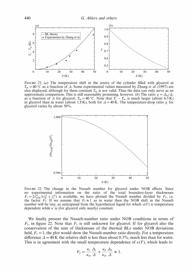
440 G. Ahlers and others
10 20 30 40 50∆ (K)
0
2
4
6
8
(a) (b)T
c –
Tm
(K
)
BL theoryExperiments by Zhang et al.
0.5
0.6
0.7
0.8
0.9
1.0
χ
10 20 30 40 50∆ (K)
0
Figure 21. (a) The temperature shift in the centre of the cylinder filled with glycerol atTm = 40 ◦C as a function of ∆. Some experimental values measured by Zhang et al. (1997) arealso displayed, although for them constant Tm is not valid. Thus the data can only serve as anapproximate comparison. This is still reasonably promising, however. (b) The ratio χ = ∆b/∆t
as a function of ∆ for glycerol; Tm =40 ◦C. Note that Tc − Tm is much larger (about 6.5 K)in glycerol than in water (about 1.8 K), both for ∆= 40 K. The temperature-drop ratio χ forglycerol varies by about 50%.
0 10 20 30 40 50∆ (K)
0.996
1.000
(Nu N
OB/N
u OB)/
F1
Figure 22. The change in the Nusselt number for glycerol under NOB effects. Sinceno experimental information on the ratio of the total boundary-layer thicknessesF1 = 2λsl
OB/(λslb + λsl
t ) is available, we have plotted the Nusselt number divided by F1, i.e.the factor F2. If we assume that F1 ≈ 1 as in water then the NOB shift in the Nusseltnumber will be tiny, as anticipated from the hypothetical liquid for which ν(T ) is temperaturedependent while κ is (for glycerol only nearly) constant.
We finally present the Nusselt-number ratio under NOB conditions in terms ofF1, in figure 22. Note that F1 is still unknown for glycerol. If for glycerol also theconservation of the sum of thicknesses of the thermal BLs under NOB deviationsheld, F1 = 1, the plot would show the Nusselt-number ratio directly. For a temperaturedifference ∆ =40 K the relative shift is less than about 0.3%, much less than for water.This is in agreement with the small temperature dependence of κ(T ), which leads to
F2 =κt
κm
∆t
∆+
κb
κm
∆b
∆≈ 1.
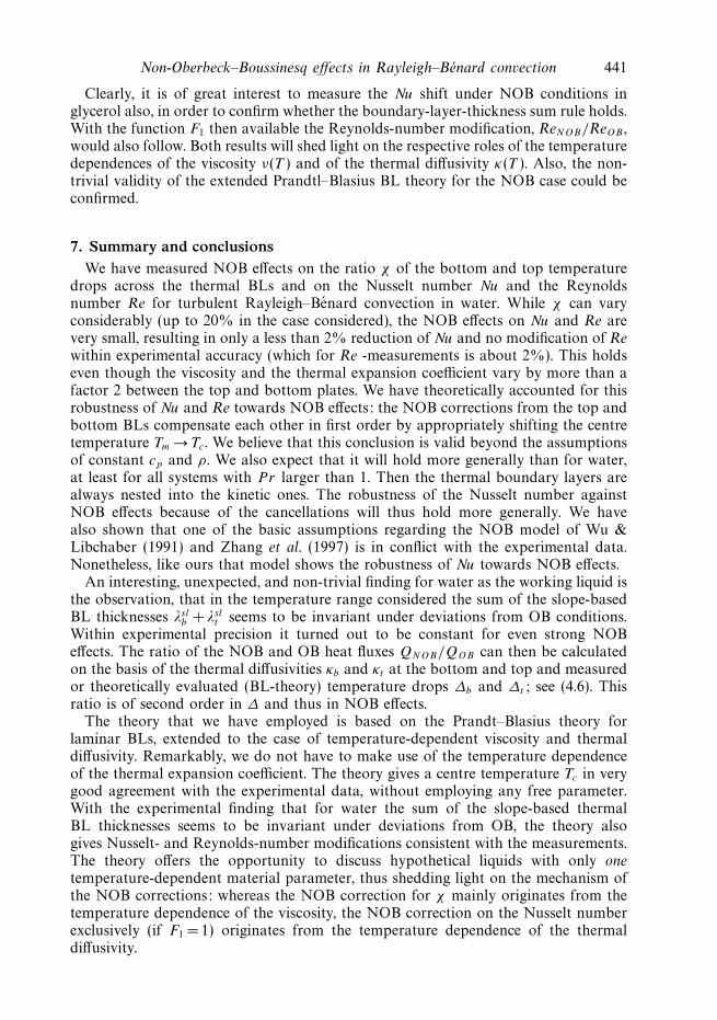
Non-Oberbeck–Boussinesq effects in Rayleigh–Benard convection 441
Clearly, it is of great interest to measure the Nu shift under NOB conditions inglycerol also, in order to confirm whether the boundary-layer-thickness sum rule holds.With the function F1 then available the Reynolds-number modification, ReNOB/ReOB ,would also follow. Both results will shed light on the respective roles of the temperaturedependences of the viscosity ν(T ) and of the thermal diffusivity κ(T ). Also, the non-trivial validity of the extended Prandtl–Blasius BL theory for the NOB case could beconfirmed.
7. Summary and conclusionsWe have measured NOB effects on the ratio χ of the bottom and top temperature
drops across the thermal BLs and on the Nusselt number Nu and the Reynoldsnumber Re for turbulent Rayleigh–Benard convection in water. While χ can varyconsiderably (up to 20% in the case considered), the NOB effects on Nu and Re arevery small, resulting in only a less than 2% reduction of Nu and no modification of Rewithin experimental accuracy (which for Re -measurements is about 2%). This holdseven though the viscosity and the thermal expansion coefficient vary by more than afactor 2 between the top and bottom plates. We have theoretically accounted for thisrobustness of Nu and Re towards NOB effects: the NOB corrections from the top andbottom BLs compensate each other in first order by appropriately shifting the centretemperature Tm → Tc. We believe that this conclusion is valid beyond the assumptionsof constant cp and ρ. We also expect that it will hold more generally than for water,at least for all systems with Pr larger than 1. Then the thermal boundary layers arealways nested into the kinetic ones. The robustness of the Nusselt number againstNOB effects because of the cancellations will thus hold more generally. We havealso shown that one of the basic assumptions regarding the NOB model of Wu &Libchaber (1991) and Zhang et al. (1997) is in conflict with the experimental data.Nonetheless, like ours that model shows the robustness of Nu towards NOB effects.
An interesting, unexpected, and non-trivial finding for water as the working liquid isthe observation, that in the temperature range considered the sum of the slope-basedBL thicknesses λsl
b + λslt seems to be invariant under deviations from OB conditions.
Within experimental precision it turned out to be constant for even strong NOBeffects. The ratio of the NOB and OB heat fluxes QNOB/QOB can then be calculatedon the basis of the thermal diffusivities κb and κt at the bottom and top and measuredor theoretically evaluated (BL-theory) temperature drops ∆b and ∆t ; see (4.6). Thisratio is of second order in ∆ and thus in NOB effects.
The theory that we have employed is based on the Prandt–Blasius theory forlaminar BLs, extended to the case of temperature-dependent viscosity and thermaldiffusivity. Remarkably, we do not have to make use of the temperature dependenceof the thermal expansion coefficient. The theory gives a centre temperature Tc in verygood agreement with the experimental data, without employing any free parameter.With the experimental finding that for water the sum of the slope-based thermalBL thicknesses seems to be invariant under deviations from OB, the theory alsogives Nusselt- and Reynolds-number modifications consistent with the measurements.The theory offers the opportunity to discuss hypothetical liquids with only onetemperature-dependent material parameter, thus shedding light on the mechanism ofthe NOB corrections: whereas the NOB correction for χ mainly originates from thetemperature dependence of the viscosity, the NOB correction on the Nusselt numberexclusively (if F1 = 1) originates from the temperature dependence of the thermaldiffusivity.
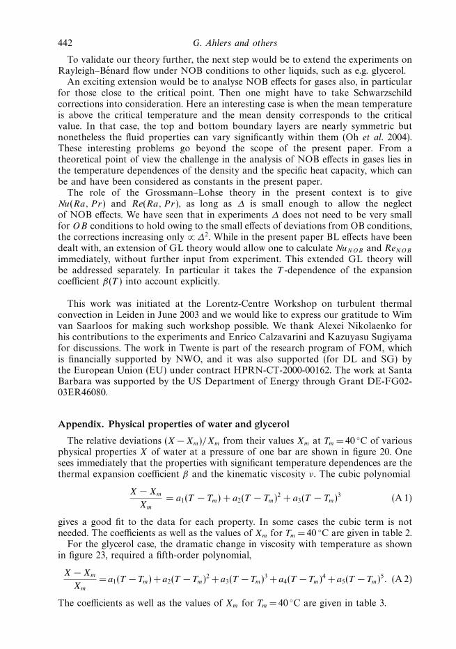
442 G. Ahlers and others
To validate our theory further, the next step would be to extend the experiments onRayleigh–Benard flow under NOB conditions to other liquids, such as e.g. glycerol.
An exciting extension would be to analyse NOB effects for gases also, in particularfor those close to the critical point. Then one might have to take Schwarzschildcorrections into consideration. Here an interesting case is when the mean temperatureis above the critical temperature and the mean density corresponds to the criticalvalue. In that case, the top and bottom boundary layers are nearly symmetric butnonetheless the fluid properties can vary significantly within them (Oh et al. 2004).These interesting problems go beyond the scope of the present paper. From atheoretical point of view the challenge in the analysis of NOB effects in gases lies inthe temperature dependences of the density and the specific heat capacity, which canbe and have been considered as constants in the present paper.
The role of the Grossmann–Lohse theory in the present context is to giveNu(Ra, P r) and Re(Ra, P r), as long as ∆ is small enough to allow the neglectof NOB effects. We have seen that in experiments ∆ does not need to be very smallfor OB conditions to hold owing to the small effects of deviations from OB conditions,the corrections increasing only ∝ ∆2. While in the present paper BL effects have beendealt with, an extension of GL theory would allow one to calculate NuNOB and ReNOB
immediately, without further input from experiment. This extended GL theory willbe addressed separately. In particular it takes the T -dependence of the expansioncoefficient β(T ) into account explicitly.
This work was initiated at the Lorentz-Centre Workshop on turbulent thermalconvection in Leiden in June 2003 and we would like to express our gratitude to Wimvan Saarloos for making such workshop possible. We thank Alexei Nikolaenko forhis contributions to the experiments and Enrico Calzavarini and Kazuyasu Sugiyamafor discussions. The work in Twente is part of the research program of FOM, whichis financially supported by NWO, and it was also supported (for DL and SG) bythe European Union (EU) under contract HPRN-CT-2000-00162. The work at SantaBarbara was supported by the US Department of Energy through Grant DE-FG02-03ER46080.
Appendix. Physical properties of water and glycerol
The relative deviations (X − Xm)/Xm from their values Xm at Tm = 40 ◦C of variousphysical properties X of water at a pressure of one bar are shown in figure 20. Onesees immediately that the properties with significant temperature dependences are thethermal expansion coefficient β and the kinematic viscosity ν. The cubic polynomial
X − Xm
Xm
= a1(T − Tm) + a2(T − Tm)2 + a3(T − Tm)3 (A 1)
gives a good fit to the data for each property. In some cases the cubic term is notneeded. The coefficients as well as the values of Xm for Tm = 40 ◦C are given in table 2.
For the glycerol case, the dramatic change in viscosity with temperature as shownin figure 23, required a fifth-order polynomial,
X − Xm
Xm
= a1(T − Tm) + a2(T − Tm)2 + a3(T − Tm)3 + a4(T − Tm)4 + a5(T − Tm)5. (A 2)
The coefficients as well as the values of Xm for Tm = 40 ◦C are given in table 3.
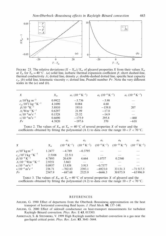
Non-Oberbeck–Boussinesq effects in Rayleigh–Benard convection 443
–20 0 20
(a) (b)
T – Tm
–20 0 20T – Tm
–0.05
0
0.05X
/Xm
– 1
ρcp
βΛ
0
10
νPr
Figure 23. The relative deviations (X − Xm)/Xm of glycerol properties X from their values Xm
at Tm for Tm = 40 ◦C . (a) solid line, isobaric thermal expansion coefficient β; short dashed-line,thermal conductivity Λ; dotted line, density ρ; double-dashed dotted line, specific heat capacitycp . (b) solid line, kinematic viscosity ν; dotted line, Prandtl number Pr . Note the very differentscales in the (a) and (b).
X Xm a1 (10−4 K−1) a2 (10−6 K−2) a3 (10−8 K−3)
ρ/103kg m−3 0.9922 −3.736 −3.98 —cp/103J kg−1K−1 4.1690 0.084 4.60 —β/10−4K−1 3.8810 195.0 −159.8 207Λ/Wm−1K−1 0.6297 21.99 −17.8 —κ/10−6m2s−1 0.1528 23.52 −14.9 —ν/10−6m2s−1 0.6690 −175.9 295.8 −460Pr 4.3820 −197.6 370 −618
Table 2. The values of Xm at Tm = 40 ◦C of several properties X of water and thecoefficients obtained by fitting the polynomial (A 1) to data over the range 10 < T < 70 ◦C.
a1 a2 a3 a4 a5
X Xm (10−4 K−1) (10−6 K−2) (10−8 K−3) (10−10 K−4) (10−12 K−5)
ρ/103 kg m−3 1.2477 −4.789 −0.3795 — — —
cp/103 J kg−1K−1
2.5108 22.511 — — — —β/10−4 K−1 4.7893 20.639 4.664 1.0757 0.2540 —Λ/10−3 Wm−1K−1 2.9351 3.863 — — — —κ/10−6 m2s−1 0.0937 13.858 3.913 −0.7577 — —ν/10−6 m2s−1 238.71 −702.83 2393.1 −6923.0 33 131.3 −71 517.5Pr 2547.9 −687.68 2325.9 −6646.3 30 875.9 −65 996.9
Table 3. The values of Xm at Tm = 40 ◦C of several properties X of glycerol and thecoefficients obtained by fitting the polynomial (A 2) to data over the range 10 < T < 70 ◦C.
REFERENCES
Ahlers, G. 1980 Effect of departures from the Oberbeck–Boussinesq approximation on the heattransport of horizontal convecting fluid layers. J. Fluid Mech. 98, 137–148.
Ahlers, G. 2000 Effect of sidewall conductance on heat-transport measurements for turbulentRayleigh–Benard convection. Phys. Rev. E 63, 015303.
Ashkenazi, S. & Steinberg, V. 1999 High Rayleigh number turbulent convection in a gas near thegas-liquid critical point. Phys. Rev. Lett. 83, 3641–3644.
444 G. Ahlers and others
Blasius, H. 1908 Grenzschichten in Flussigkeiten mit kleiner Reibung. Z. Math. Phys. 56, 1–37.
Bodenschatz, E., deBruyn, J., Ahlers, G. & Cannell, D. 1991 Transition between patterns inthermal convection. Phys. Rev. Lett. 67, 3078–3081.
Bodenschatz, E., Pesch, W. & Ahlers, G. 2000 Recent developments in Rayleigh–Benardconvection. Annu. Rev. Fluid Mech. 32, 709–778.
Boussinesq, J. 1903 Theorie Analytique de la Chaleur, Vol. 2 . Gauthier-Villars.
Brown, E., Funfschilling, D. & Ahlers, G. 2006 Reynolds numbers of the large-scale flow inturbulent Rayleigh–Benard convection. unpublished .
Brown, E., Funfschilling, D., Nikolaenko, A. & Ahlers, G. 2005 Heat transport by turbulentRayleigh–Benard convection: Effect of finite top- and bottom conductivity. Phys. Fluids 17,075108.
Busse, F. H. 1967 The stability of finite amplitude cellular convection and its relation to anextremum principle. J. Fluid Mech. 30, 625–649.
Castaing, B., Gunaratne, G., Heslot, F., Kadanoff, L., Libchaber, A., Thomae, S., Wu, X. Z.,
Zaleski, S. & Zanetti, G. 1989 Scaling of hard thermal turbulence in Rayleigh–Benardconvection. J. Fluid Mech. 204, 1–30.
Chaumat, S., Castaing, B. & Chilla, F. 2002 Rayleigh–Benard cells: influence of plate properties.In Advances in Turbulence IX (ed. I. P. Castro & P. E. Hancock). Barcelona: InternationalCentre for Numerical Methods in Engineering, CIMNE.
Chavanne, X., Chilla, F., Castaing, B., Hebral, B., Chabaud, B. & Chaussy, J. 1997 Observationof the ultimate regime in Rayleigh–Benard convection. Phys. Rev. Lett. 79, 3648–3651.
Chavanne, X., Chilla, F., Chabaud, B., Castaing, B. & Hebral, B. 2001 Turbulent Rayleigh–Benard convection in gaseous and liquid He. Phys. Fluids 13, 1300–1320.
Chilla, F., Rastello, M., Chaumat, S. & Castaing, B. 2004 Long relaxation times and tiltsensitivity in Rayleigh–Benard turbulence. Euro. Phys. J. B 40, 223–227.
Ciliberto, S., Pampaloni, E. & Perez–Garcia, C. 1988 Competition between different symmetriesin convective patterns. Phys. Rev. Lett. 61, 1198–1201.
Funfschilling, D., Brown, E., Nikolaenko, A. & Ahlers, G. 2005 Heat transport by turbulentRayleigh–Benard convection in cylindrical cells with aspect ratio one and larger. J. FluidMech. 536, 145–154.
Furukawa, A. & Onuki, A. 2002 Convective heat transport in compressible fluids. Phys. Rev. E 66,016302.
Gitterman, M. 1978 Hydrodynamics of fluids near a critical point. Rev. Mod. Phys. 50, 85–107.
Gitterman, M. & Steinberg, V. 1971 Criteria of occurrence of free convection in a compressibleviscous heat-conducting fluid. J. Appl. Math. Mech. (USSR) 34, 305–311.
Grossmann, S. & Lohse, D. 2000 Scaling in thermal convection: A unifying view. J. Fluid Mech.407, 27–56.
Grossmann, S. & Lohse, D. 2001 Thermal convection for large Prandtl number. Phys. Rev. Lett.86, 3316–3319.
Grossmann, S. & Lohse, D. 2002 Prandtl and Rayleigh number dependence of the Reynoldsnumber in turbulent thermal convection. Phys. Rev. E 66, 016305.
Grossmann, S. & Lohse, D. 2004 Fluctuations in turbulent Rayleigh–Benard convection: The roleof plumes. Phys. Fluids 16, 4462–4472.
Hoard, C., Robertson, C. & Acrivos, A. 1970 Experiments on the cellular structure in Benardconvection. Intl. J. Heat Mass Transfer 13, 849–856.
Kogan, A. & Meyer, H. 2001 Heat transfer and convection onset in a compressible fluid: 3He nearthe critical point. Phys. Rev. E 63, 056310:1–15.
Kraichnan, R. H. 1962 Turbulent thermal convection at arbritrary Prandtl number. Phys. Fluids5, 1374–1389.
Landau, L. D. & Lifshitz, E. M. 1987 Fluid Mechanics . Pergamon.
Meksyn, D. 1961 New Methods in Laminar Boundary Layer Theory . Pergamon.
Niemela, J., Skrebek, L., Sreenivasan, K. R. & Donnelly, R. J. 2000 Turbulent convection atvery high Rayleigh numbers. Nature 404, 837–840.
Niemela, J., Skrbek, L., Sreenivasan, K. R. & Donnelly, R. J. 2001 The wind in confined thermalturbulence. J. Fluid Mech. 449, 169–178.
Niemela, J. & Sreenivasan, K. R. 2003 Confined turbulent convection. J. Fluid Mech. 481,355–384.
Non-Oberbeck–Boussinesq effects in Rayleigh–Benard convection 445
Nikolaenko, A., Brown, E., Funfschilling, D. & Ahlers, G. 2005 Heat transport by turbulentRayleigh–Benard convection in cylindrical cells with aspect ratio one and less. J. Fluid Mech.523, 251–260.
Oberbeck, A. 1879 Uber die Warmeleitung der Flussigkeiten bei Berucksichtigung der Stromungeninfolge von Temperaturdifferenzen. Ann. Phys. Chem. 7, 271–292.
Oh, J., Ortiz de Zarate, J. M., Sengers, J. V. & Ahlers, G. 2004 Dynamics of fluctuations in afluid below the onset of Rayleigh–Benard convection. Phys. Rev. E 69, 021106.
Pampaloni, E., Perez–Garcia, C., Albavetti, L. & Ciliberto, S. 1992 Transition from hexagonsto rolls in convection in fluids under non-Boussinesq conditions. J. Fluid Mech. 234, 393–416.
Plapp, J. E. 1957 Laminar free convection with variable fluid properties. PhD thesis, Caltech,available at http://resolver.caltech.edu/CaltechETD:etd-09142004-153230.
Pohlhausen, E. 1921 Der Wameaustausch zwischen Festkorpern und Flussigkeiten mit kleinerReibung und kleiner Warmeleitung. Z. Angew. Math. Mech. 1, 115–121.
Prandtl, L. 1905 Uber Flussigkeitsbewegung bei sehr kleiner Reibung , pp. 484–491. Leipzig: Teubner.
Press, W., Teukolsky, S., Vetterling, W. & Flannery, B. 1986 Numerical Recipes . CambridgeUniversity Press.
Qiu, X. L. & Tong, P. 2001a Large scale velocity structures in turbulent thermal convection. Phys.Rev. E 64, 036304.
Qiu, X. L. & Tong, P. 2001b Onset of coherent oscillations in turbulent Rayleigh–Benard convection.Phys. Rev. Lett . 87, 094501.
Roche, P. E., Castaing, B., Chabaud, B. & Hebral, B. 2001 Observation of the 1/2 power law inRayleigh–Benard convection. Phys. Rev. E 63, 045303.
Roche, P. E., Castaing, B., Chabaud, B. & Hebral, B. 2002 Prandtl and Rayleigh numbersdependences in Rayleigh–Benard convection. Europhys. Lett. 58, 693–698.
Schlichting, H. & Gersten, K. 2000 Boundary Layer Theory , 8th edn. Springer.
Shraiman, B. I. & Siggia, E. D. 1990 Heat transport in high-Rayleigh number convection. Phys.Rev. A 42, 3650–3653.
Sun, C., Ren, L.Y., Song, H., and Xia, K.Q. 2005 Heat transport by turbulent Rayleigh-Benardconvection in 1m diameter cylindrical cells of widely varying aspect ratio. J. Fluid Mech. 542,165–174.
Verzicco, R. 2002 Sidewall finite conductivity effects in confined turbulent thermal convection. J.Fluid Mech. 473, 201–210.
Verzicco, R. 2004 Effect of non-perfect thermal sources in turbulent thermal convection. Phys.Fluids 16, 1965–1979.
Walden, R. W. & Ahlers, G. 1981 Non-Boussinesq and penetrative convection in a cylindricalcell. J. Fluid Mech. 109, 89–114.
Wall, D. P. & Wilson, S. K. 1997 The linear stability of flat-plate boundary-layer flow of fluidwith temperature-dependent viscosity. Phys. Fluids 9, 2885–2898.
Wu, X. Z. & Libchaber, A. 1991 Non-Boussinesq effects in free thermal convection. Phys. Rev. A43, 2833–2839.
Xu, X., Bajaj, K. M. S. & Ahlers, G. 2000 Heat transport in turbulent Rayleigh–Benard convection.Phys. Rev. Lett. 84, 4357–4360.
Zhang, J., Childress, S. & Libchaber, A. 1997 Non-Boussinesq effect: Thermal convection withbroken symmetry. Phys. Fluids 9, 1034–1042.


![On Chorin’s method for stationary solutions of the Oberbeck ...A. Chorin ([2, 3, 4]) proposed the arti cial compressible system such as (1.4){(1.6) to nd stationary solutions of](https://img.pdfslide.us/doc/110x75/5ff11ce737511c6888028dd5/on-chorinas-method-for-stationary-solutions-of-the-oberbeck-a-chorin-2.jpg)
![Modeling the provenance of the Apollo 16 regolith · contrast, Oberbeck et al. [1974] utilized ejecta mixing equations in concluding that the Imbrium basin was the dominant basin](https://img.pdfslide.us/doc/110x75/60af34284738b26f3e4c5191/modeling-the-provenance-of-the-apollo-16-contrast-oberbeck-et-al-1974-utilized.jpg)

![The Nature of Crater Rays: The Copernicus Examplepmm/CopernicusJGR.pdf · Oberbeck [1971] studied high-resolution Lunar Orbiter images of a ray element southeast of Copernicus and](https://img.pdfslide.us/doc/110x75/60af34284738b26f3e4c5192/the-nature-of-crater-rays-the-copernicus-example-pmmcopernicusjgrpdf-oberbeck.jpg)