Embed Size (px)
Citation preview
Department of Economics
School of Business, Economics and Law at University of Gothenburg
Vasagatan 1, PO Box 640, SE 405 30 Göteborg, Sweden
+46 31 786 0000, +46 31 786 1326 (fax)
www.handels.gu.se [email protected]
WORKING PAPERS IN ECONOMICS
No 588
Non-Monotonic Health Behaviours
- implications for individual health-related behaviour
in a demand-for-health framework
Kristian Bolin & Björn Lindgren
March 2014
ISSN 1403-2473 (print) ISSN 1403-2465 (online)
1
NON-MONOTONIC HEALTH BEHAVIOURS –
implications for individual health-related behaviour in a
demand-for-health framework*
KRISTIAN BOLIN1,2
BJÖRN LINDGREN2,3,4
1 Department of Economics, University of Gothenburg, Gothenburg, Sweden
2 Centre for Health Economics, University of Gothenburg, Gothenburg, Sweden
3 Department of Health Sciences, Lund University, Lund, Sweden
4 National Bureau of Economic Research (NBER), Cambridge MA, United States
ABSTRACT
A number of behaviours influence health in a non-monotonic way. Physical activity and alcohol consumption, for instance, may be beneficial to one’s health in moderate but detrimental in large quantities. We develop a demand-for-health framework that incorporates the feature of a physiologically optimal level. An individual may still choose a physiologically non-optimal level, because of the trade-off in his or her preferences for health versus other utility-affecting commodities. However, any deviation from the physiologically optimal level will be punished with respect to health. A set of steady-state comparative statics is derived regarding the effects on the demand for health and health-related behaviour, indicating that individuals will react differently to exogenous changes, depending on the amount of the health-related behaviour they demand. We also show (a) that a steady-state equilibrium is a saddle-point and (b) that the physiologically optimal level may be a steady-state equilibrium for the individual. Our analysis suggests that general public-health policies may, to some extent, be counterproductive due to the responses induced in parts of the population.
Keywords: Human capital; Grossman model; non-monotonic health investments; health; steady-
state and stable equilibria.
JEL classification: I12
2
1. INTRODUCTION
Most human behaviours are related to health. Individual health affects consumption patterns, but
consumption patterns also affect individual health. While the sole intention of health-care
utilisation is either to improve current health, whenever it has fallen below a certain illness-
defining threshold value, or to prevent future illness, rather than to consume it for the sake of its
direct utility (which might even be negative), the intention of many other behaviours may be
twofold: both to gain direct consumption utility and to improve health (or to decrease the risk of
illness). The latter category includes, for instance, physical exercise, certain consumption and
composition of food, alcohol consumption and, as a matter of fact, any recreational activity (art,
literature, music, etc). Obviously, health effects may be more or less intentional, and certain
consumption patterns may also be detrimental to your health. Smoking is an unambiguous
example of the latter.
Smoking is always bad for your health – and increasingly so with increased consumption (Doll et
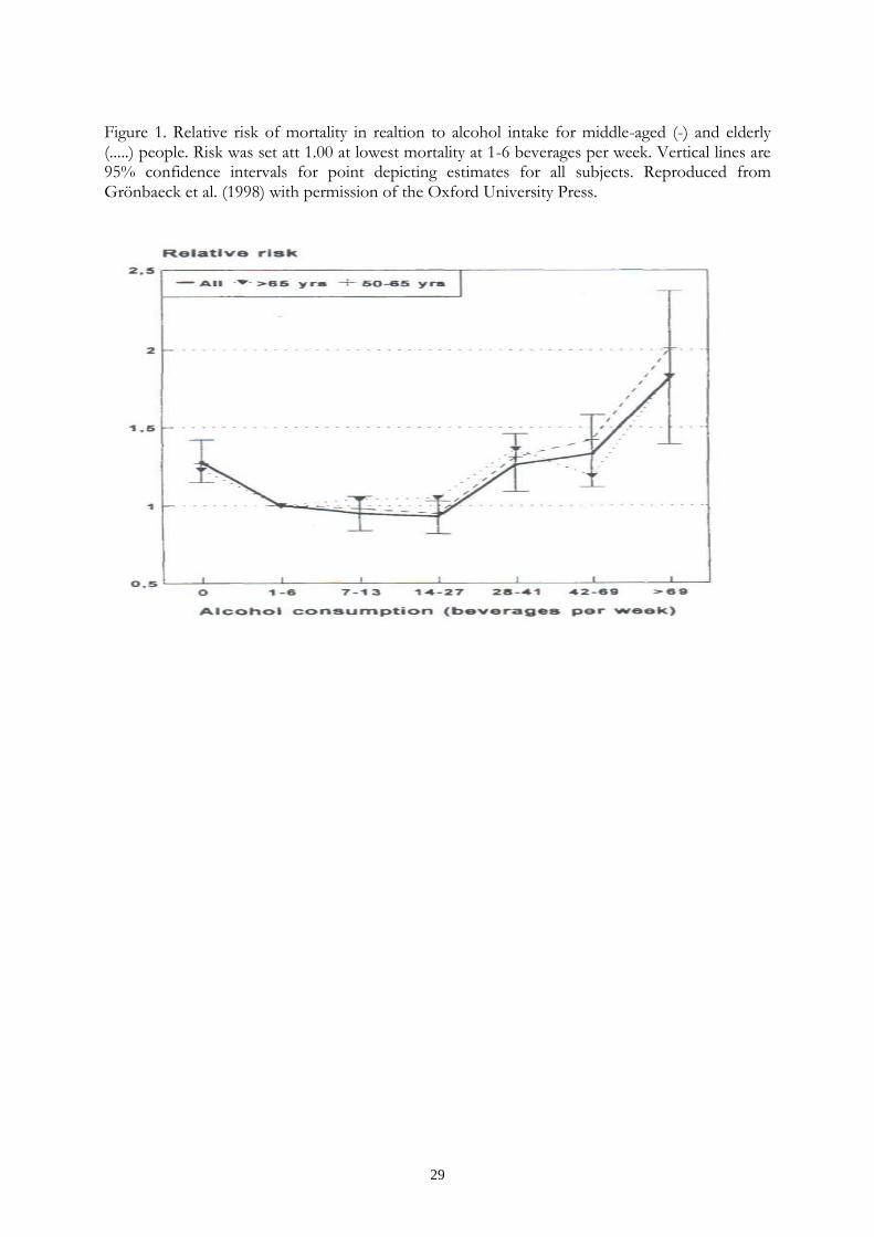
al, 1976; Doll et al, 1994; Colditz, 2000; Vineis et al, 2004). In contrast, there appears to be a
physiologically determined, individually optimal level of activity (greater than zero) as regards, for
instance, physical exercise, food intake, alcohol consumption, and sleep, implying that activity
levels below or above that level would result in a level of health which is lower than the
maximum achievable level; see Figure 1 for an illustrative example of a typically U-shaped
relation.
Figure 1 about here
A consistently positive association between physical-activity level and health-related quality of life
has been found (Bize et al, 2007). Certainly, too small amounts of physical exercise means that
3
the human body atrophies and that the risks of several diseases, including coronary heart disease,
hypertension, stroke, diabetes, depression, osteoporosis, and cancers of the breast and colon,
increase (Garrett et al, 2004). However, too much or too intensive physical exercise means that
the human body will wear down and/or that the risk of injury increases (Tisi and Shearman,
1998; Locke, 1999; Ji, 2001; Randolph, 2007; Howatson G and van Someren, 2008; Morton et al,
2009). A varied and balanced diet is emphasised in guidelines on healthy eating; see, for instance
(Swedish National Food Agency, 2012). Too little food or too one-sided diet lead to health
problems (Steinhausen, 2002). Too much also creates health problems (Steinhausen and Weber,
2009), in particular in combination with too little physical exercise.
Overweight (25 ≤ BMI < 30)1 and obesity (BMI ≥ 30) increase the risks of asthma, coronary
heart disease, hypertension, diabetes, osteoarthritis, and cancer, including cancers of the breast
and colon (Colditz, 1999; Must et al., 1999); Dal Grande, 2009). Also underweight (BMI < 18.5)
has been shown to be associated with health problems; for instance, coronary heart disease,
diabetes, and gallbladder disease (Must et al., 1999). Light to moderate drinkers are at lower risk
of coronary heart disease, stroke, diabetes, and gallstone disease than non-drinkers, while an
increasing intake increases the risks of dementia, liver cirrhosis, pancreatitis, osteoporosis, and
most cancers, including cancer of the oesophagus, breast, pancreas, colon, and rectum
(Grönbaeck, 2009). Finally, both short and long sleep durations appear to be related to increased
likelihood of obesity, diabetes, hypertension, and cardiovascular disease (Buxton and Marcelli,
2010; Sabanayagam and Shankar, 2010).
It should be emphasised, though, that which level of physical exercise, food intake, alcohol
consumption, and sleep is physiologically optimal differs among individuals, and if you have
* We thank Martin Forster for insightful comments and useful suggestions. 1 BMI (body mass index) is calculated as weight in kilograms divided by height in meters.
4
good genes and/or are lucky, you may suffer less from “unhealthy” behaviour than less
advantaged people.
In general terms, these associations have been known for decades. Yet, there are no clear
temporal trends worldwide towards healthier life-styles (Knuth and Hallai, 2009), and the
population variance of these behaviours is large; for instance, many people do not perform any,
or very little, physical exercise, others perform very large amounts. We will demonstrate that such
polarization may be possible to explain, within a modified version of Grossman’s demand-for-
health model, assuming that there is a (strictly positive) physiologically optimal level of the
corresponding health behaviour.
The demand-for-health model extended the human capital theory by explicitly incorporating
health and recognising that there are both consumption and investment motives for investing in
health (Grossman, 1972a, b). It resulted in an economic theory of individual health-related
behaviour. The basic features of the model are (1) that the individual demands health (a) for its
utility enhancing effects (the consumption motive), and (b) for its effect on the amount of
healthy time (the investments motive), (2) that the demand for investments in health is derived
from the more fundamental demand for health, (3) that the investments in health are produced
by the individual, and (4) that the stock of health depreciates at each point in time. The
production aspect implies that the produced amount of investments in health has to be
assimilated by the individual. Thus, the effects of, for instance, physical exercise, is assimilated
and transformed into health by the individual at rates that differ between individuals. This goes
beyond the effect of the depreciation of the stock of health at each point in time.
Although some variance in health-related behaviours may be readily understood within
Grossman’s original version of the demand-for-health model, the observed variance seems to be
5
greater than what would be expected, solely taken the variability in physiologically determined,
individually optimal level of activity into account. In this paper we develop a version of
Grossman’s demand-for-health model, modified in order to focus on individually optimal choices
of health-related behaviour, distinguished by physiologically optimal activity levels.
Since its introduction, the demand-for-health model has been extended in various ways;
incorporating risk and uncertainty (Dardanoni and Wagstaff, 1987, 1990; Selden, 1993; Chang,
1996; Liljas, 1998, 2000; Picone et al., 1998; Asano and Shibata, 2011), the family as producer of
health (Jacobson, 2000; Bolin et al., 2001, 2002b), the employer as producer of health (Bolin et
al., 2002c), social capital (Bolin et al., 2003), healthy and unhealthy consumption (Forster, 2001),
decreasing returns to scale in the production of health investment (Ehrlich and Chuma, 1990;
Galama, 2011), imperfect financial markets (Liljas, 2000, 2002), and allowing for corner solutions
(Galama and Kapteyn, 2011). To our knowledge, however, the effect on the demand for health
and health investments of the double-facetted nature of individual behaviours with
physiologically determined optimal levels as regards health and negative or positive health effects,
depending on the level of activity, has never been analysed.2 While the emphasis of the paper is
on extending theory, it will be shown that such an analysis has important implications for the
understanding of individual health-related behaviour and, hence, for designing and evaluating
health policies.
The structure of the rest of the paper is as follows. Next, we will present the model. After that,
we will derive the optimality conditions. Following this, we will analyse the properties of the
2 Forster (2001) studied health-related effects of there being two types of consumption: good for health and bad for health. In both cases the effect on health is monotonic in consumption. In our case, the relationship between the amount of behaviour and its health effect is not monotonic. Grossman (1972a) examined the importance of joint production in the production of gross health investment. He argued that several goods are demanded as inputs into the production of commodities, other than health, that yield utility but may have adverse health effects.
6
dynamic system in terms of steady-state and stability conditions. The final section contains a
discussion and some conclusions.
2. THE MODEL
Our theoretical model takes its departure in the demand-for-health model developed by Michael
Grossman (1972a, b). It differs from Grossman’s original formulation mainly (1) by avoiding an
explicit treatment of the individual’s time allocation problem3, and (2) by considering health-
related behaviours that are not monotonic in their effect on health.
2.1 Preferences
We consider a version of the demand-for-health model in continuous time, in which health at
each point in time, , is produced by the individual through a specific health behaviour, .
The behaviour influences health positively below a certain level, and negatively above that
level; we assume that the smallest amount of behaviour is zero. The individual derives utility
from his or her stock of health, , from health-related behaviour, , as well as from
consumption unrelated to health, . More specifically, we assume that preferences are
additively separable, time additive, and concave in all arguments. In order to reduce complexity
and, hence, to increase the capability of the model to generate unambiguous predictions, we also
assume that the marginal utility of (the health-unrelated) consumption is constant. Further,
throughout the paper we deal with individuals that choose strictly positive levels of the -
behaviour but spend strictly less than total available resources on , i.e., ,
where is defined as the level of where the utility of an additional unit of is exactly
balanced by the reduction in utility brought about by the necessary reduction in the consumption
of , dictated by the budget restriction. Formally, individual preferences are represented by the
3 Instead, we utilise the individual’s cost function, pertaining to the allocation problem that he or she faces. This means that we – implicitly – assume that the individual has solved the time allocation problem.
7
following quasi-linear continuous utility function (
and )4,5:
( ) ( ) (1)
where is the marginal utility of consumption.
The positive health effect produced by the behaviour, , is partially offset by a natural
depreciation – at rate – of the existing stock of health capital.6 For tractability of
dynamic analysis we consider a model in which the rate of depreciation is time independent.7
Further, we distinguish between the ability to produce (see below) the behaviour, , and the
rate at which the behaviour is transformed into gross health investments, . Thus, the
equation of motion for the stock of health capital is:
. (2)
This equation comprises two sources of bodily decay: the natural depreciation, by rate , which
can be compensated for by the health-related behaviour, , and atrophy of the body, which can be
avoided – at there is no atrophy. This level of the -behaviour reflects the amount by
which the body atrophies, when the individual does not partake in the healthy behaviour, i.e.,
when . At the zero activity level, the body atrophies at the rate ; the parameter
( ) reflects the rate at which the individual may reduce the amount of atrophy by
4 Throughout the paper, a subscript indicates a partial derivative. Deviating somewhat from established practice, we
denote the time derivative as
.
5 Quasi-linear utility functions have been extensively applied in economic analyses of the family, and related issues; see, for instance, Chang (2009, 2007); Chang and Weisman (2005); Konrad et al., (2002); Konrad and Lommerud (2000). Essentially, the quasi-linearity assumption means that the analysis is focused on the importance of relative prices, since there is no income effect for goods other than the linear-utility good. 6 Fundamentally, one may argue that the health-related behaviour is an input into the production of gross health investments and not the output of that production process. In an analysis of the composition of inputs into the production of gross health investments, this distinction would be necessary. Here, however, our focus is on the effects of a specific behaviour, having a negatively U-shaped effect on health. 7 In this paper, we analyse time-paths and stability of equilibrium. This is considerably less difficult in autonomous systems, which require a time-independent rate of depreciation, or that total depreciation at each point in time is independent of the health stock. This is in contrast to Grossman (1972), Muurinen (1982), Wagstaff (1986), Liljas (1998), Jacobson (2000), and Bolin et al. (2001a), who all examined models with time-dependent rates of depreciation.
8
modifying the -behaviour. Different behaviours are characterised by different 's. Starting at
and moving towards more -behaviour will gradually offset the atrophy until it is
exactly balanced at
√
. At
, the -behaviour exerts its
maximum health-enhancing effect:
. Thus,
is the
physiologically optimal level of the -behaviour. Increasing beyond that point will start to
reduce the health effect of the behaviour.
Figure 2 about here
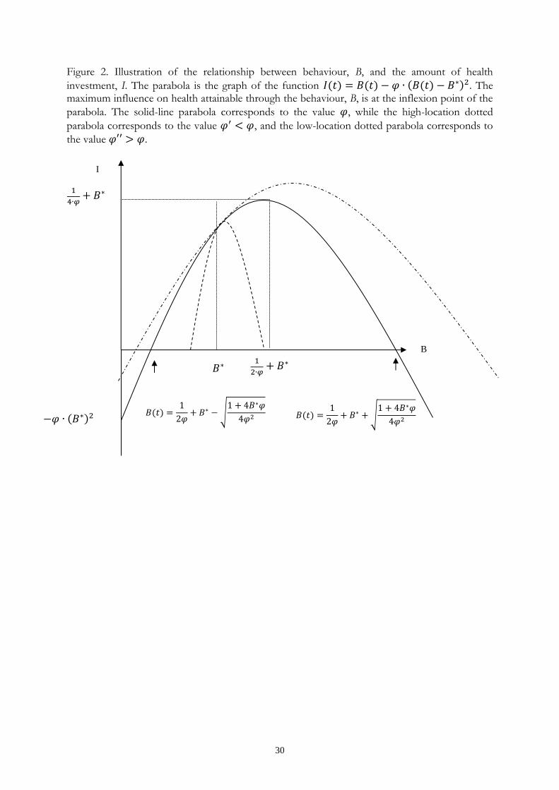
Figure 2 illustrates the influence on gross health investment produced by the -behaviour. It
facilitates our analysis to distinguish between three individual types: those that exert less and
more, respectively, than the physiologically optimal level,
, and those that exert exactly
the physiologically optimal level – these types will be referred to as type 1, 2 and 3. A higher rate
at which the atrophy increases when the individual moves away from implies (1) that the
physiologically optimal level of moves closer to , and (2) that the level of that exactly
offsets atrophy or adverse health effects moves closer to (the distance between the
intersections with the horizontal axis and gets smaller).
2.2 Production technology and cost function
For simplicity, we assume that the technology used for producing the health-related behaviour is
homogenous and exhibits constant returns to scale. Thus, the technology is formally represented
by a production function that is homogenous, of degree 1 in the quantity of investment. Thus,
the dual cost-of-behaviour function is homogenous of degree 1 with respect to the quantity of
9
the behaviour, i.e., the cost of producing the behaviour is constant with respect to its quantity.
Formally, the cost function is:
, (3)
where is the one-unit cost of producing the behaviour, is the composite price of
market goods and services used in the production, is the wage rate, and is the level of
knowledge. Thus, differences between individuals regarding their production efficiencies are
comprised in and .
2.3 Budget constraint
For convenience, we assume that there are no financial markets and, hence, that total spending at
time equals market income at time .8 Hence, the individual's budget constraint can be
expressed as:
( ) , (4)
where denotes full market income (the market value of total time that is available for market
work or the -behaviour), and the price of the consumption good. We express full market
income as a function of health, since health determines the total amount of time, which is
available for the individual to allocate between and market work. This amount of time equals
total time, , reduced by time spent being sick, . Thus, full market income is:
( ). (5)
Available time that the individual may allocate freely between its two productive uses increases as
the stock of health capital increases. Formally, the amount of time spent being sick is inversely 8 In this way an autonomous dynamic model is obtained without introducing time as yet another state variable. Analysing properties of non-autonomous dynamic system is beyond what can be achieved using most economists’ tool box. Autonomous systems are considerably more straightforward, while still allowing for important issues to be analysed. Dynamic models of health behaviour, when there are no financial markets, have been used by, for instance, Liljas (1998) and Forster (2001). Here, the absence of capital markets means that the only way that the individual can transfer resources between different points in time is by investing in health capital. We have made the assumption that preferences, prices, technology and the rate of depreciation are time invariant, which means that individual incentives for transferring resources between stages of the lifecycle do not comprise any timing-of-investment considerations. With time-varying prices for the inputs into production of health capital, this would be a major purpose for transferring resources in time.
10
related to the stock of health capital, i.e., . Further, we assume that the productivity of
health in producing healthy time is diminishing, i.e., , at a constant rate, i.e., .
Thus, potential income is increasing and concave in health capital, since ;
and .
2.4 The individual’s control problem
The individual's objective is to maximize his or her lifetime utility. Formally, this means solving
the intertemporal optimization problem of choosing the time path of health capital that
maximizes lifetime utility by partaking optimally in the health-related behaviour. We assume a
fixed end-point for the individual’s planning horizon and that the shadow price of health capital
must be 0 at , or that equals the smallest permitted health level. Thus, discounting
future utility at the rate , the individual acts as if solving the following problem:9
∫ [ ( ) ( ) ]
(6)
subject to:
,
and the transversality condition ( ) , where is the smallest
permissible level of health. The individual inherits a known stock of health , i.e., .
3 RESULTS
3.1 Conditions for optimal paths of behaviour and health
The solution to the maximisation problem is obtained by means of the maximum principle of
optimal control theory, which gives necessary and sufficient conditions for the optimal control of
9 For convenience, we formulate the individual’s optimisation problem as a vertical terminal line problem, which means that the terminal time is fixed, but the terminal state is free (Chiang, 1992, p.182). This is to be distinguished from a horizontal terminal line problem in which the terminal time, T, is free, and, hence, that the terminal state is
restricted to . The optimality conditions resulting from these two problems only differ regarding the
transversality conditions. In the horizontal terminal line problem, optimal length of life is, implicitly, determined by the transversality conditions; see, for instance, Ehrlich and Chuma (1990). The individual’s life-time optimisation problem was formulated as a vertical time line problem by, for instance, Bolin et al (2001; 2002b, c).
11
, given the time path of the state variable .10 The current-value Hamilton function for
the maximisation problem is, substituting for using (4):
( ) ( ) ( )
(7)
The maximum principle yields the following equations of motion. First, for the stock of health:
(8)
The optimal choice of the single control variable, , satisfies the first-order (sufficient)
condition:
( ) . (9)
The optimal level of the -behaviour
Let us begin by restating a useful result: since , we know that [ ]
(Caputo, 2005; p. 56) and, hence, optimal choices can be analysed, for each type, by using the
sign of
. Thus, condition (9) implies that the type-1 individual partakes in the -
behaviour at a level
, where is defined by ( )
. Similarly,
the type-2 individual partakes at a level
, where is defined by ( )
. This is clear from, first, the assumption that for both types:
| ; and, second, the definition of the type-1 individual (
)
|
(analogously for type 2). Thus, due to continuity we are assured that
for some , such that
, |
. Similarly, for the type-2
10 By the Mangasarian sufficiency theorem, (8) and (9) are necessary and sufficient conditions for an optimum if the
Hamiltonian function, , is jointly and strictly concave in . First, notice that . That leaves
only the diagonal terms of the Hessian matrix, , for the Hamiltonian function. These are: , and , which means that | | > 0 and, hence, that the Hamiltonian is jointly
and strictly concave in .
12
individual we have |
, and | . Then, since, by assumption, is
affordable, we are guaranteed that for some , such that
,
| . Finally, a necessary and sufficient condition for optimal behaviour for a type-3
individual is: (
)
.
3.2 Phase diagrams
In this section we will explore the qualitative properties of possible solutions to the optimization
problem (6). The phase diagrams (in state-control space) that we use distinguish between the
three individual types. We begin by tracing out the
and
loci for all three types
in the same diagram. Let denote the equation of motion for
. (10)
In order to obtain the corresponding equation of motion for , take the total time derivative
of (9), and solve for
, which yields:
( ) ,
and, setting
:
( )
(11)
where is defined by (8). The dynamics of the system is described by equations (10) and (11).
The isoclines can be found by setting . Let us begin with the
locus,
for which it is possible to obtain an explicit expression. Rearranging the equation
yields:
⁄
. Figure 3 illustrates the principal shapes of the
loci. The graphs drawn in the figure are obtained as follows: is a parabola having a vertex
(
at
, and intersections with the B-axis at
13
√
. Notice that if the steady-state behaviour is , equation (2) implies that the
steady-state health stock is
. In the appendix, we show that the
locus has one
branch at each side of
, and that it is decreasing in the left branch, increasing in
the right, and concave in both. From equation (11) it is clear that a third
locus is
. When changes, the
locus will change in the same way as the graph
of in Figure 2.
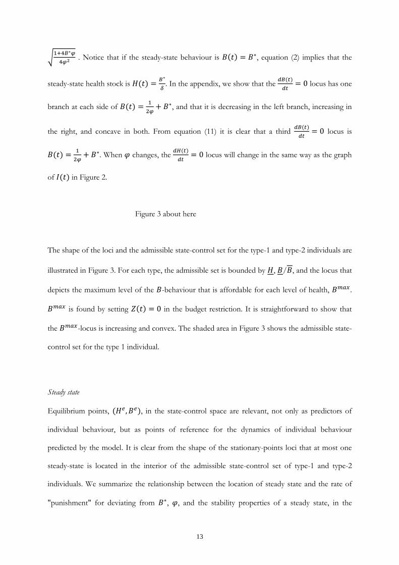
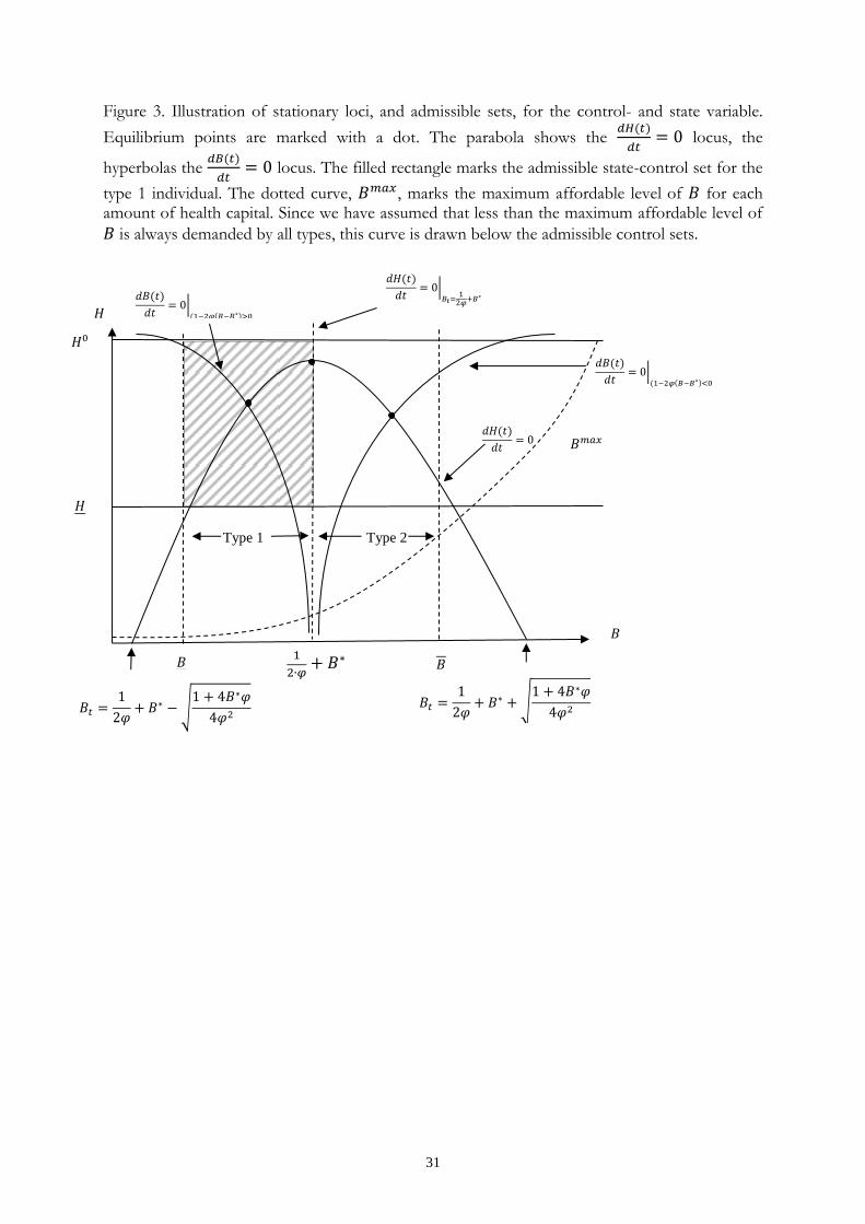
Figure 3 about here The shape of the loci and the admissible state-control set for the type-1 and type-2 individuals are
illustrated in Figure 3. For each type, the admissible set is bounded by , / , and the locus that
depicts the maximum level of the -behaviour that is affordable for each level of health, .
is found by setting in the budget restriction. It is straightforward to show that
the -locus is increasing and convex. The shaded area in Figure 3 shows the admissible state-
control set for the type 1 individual.
Steady state
Equilibrium points, , in the state-control space are relevant, not only as predictors of
individual behaviour, but as points of reference for the dynamics of individual behaviour
predicted by the model. It is clear from the shape of the stationary-points loci that at most one
steady-state is located in the interior of the admissible state-control set of type-1 and type-2
individuals. We summarize the relationship between the location of steady state and the rate of
"punishment" for deviating from , , and the stability properties of a steady state, in the
14
following two claims (additional comparative-statics results, with respect to other parameters of
the model, are reported in the appendix):
Claim 1: the effects on steady state of an increase in are:
(i) for type 1:
( when );
when ( when ); and
when
;
(ii) for type 2:
and
; and
(iii) for type 3:
and
.
Proof: The proof is a straightforward comparative-static computation. See appendix.
The stability properties of steady state are summarized in Claim 2:
Claim 2: a steady state is saddle-point stable for types 1 and 2, and globally stable for type 3.
Proof: See appendix.
The intuition behind the results for the type-1 individual is as follows. First, consider the case
when : then an increase in the rate at which deviating from is “punished” will have
a negative impact on the equilibrium demand for health capital, since each amount of will
produce a smaller amount of gross investments in health. However, when the health stock
decreases, the marginal utility value of future health capital produced by goes up, due to
( ) (both and increases), which means that the marginal
instantaneous utility of must also increase (due to (9)). Thus, must increase in this case.
Second, when
, the marginal utility value of future health capital produced
by may increase or decrease, since ( ) decreases. The intuition for
the type-2 individual is analogous.
15
3.3 Trajectories and solutions
The dynamic properties of the model for different points in the state-control space can be
expressed using and . Taking the derivative with respect to of respective function,
leaving out the arguments, results in and ( )
when
. This means that
below the
locus, and
,
above it; and, further, that
below the
locus when
.
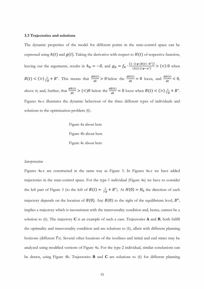
Figures 4a-c illustrates the dynamic behaviour of the three different types of individuals and
solutions to the optimization problem (6).
Figure 4a about here
Figure 4b about here
Figure 4c about here
Interpretation
Figures 4a-c are constructed in the same way as Figure 3. In Figures 4a-c we have added
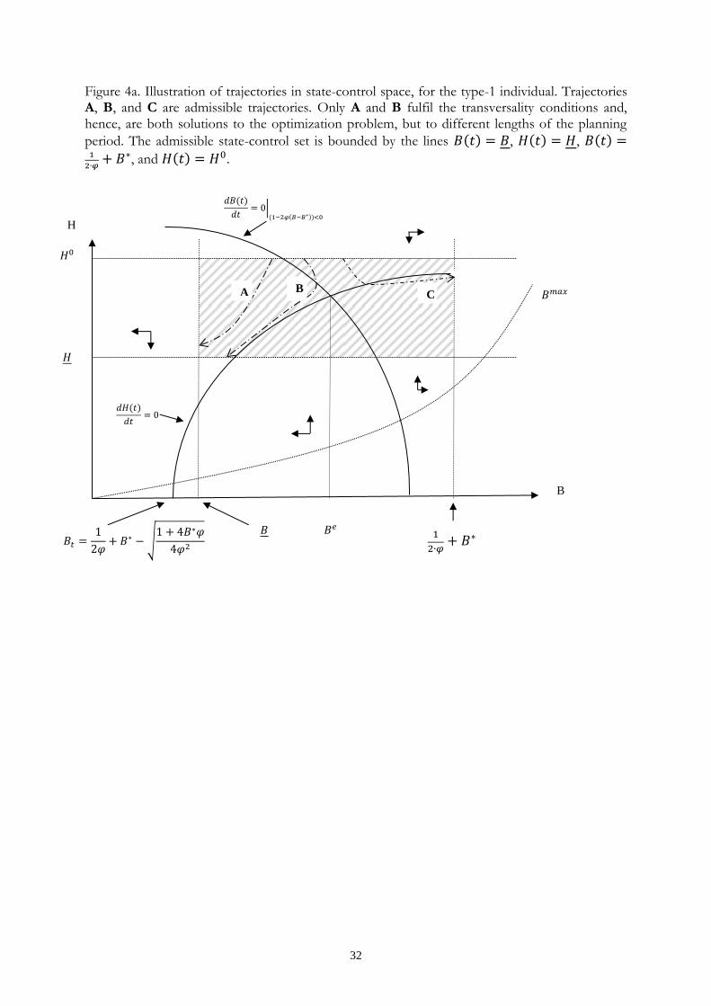
trajectories in the state-control space. For the type-1 individual (Figure 4a) we have to consider
the left part of Figure 3 (to the left of
). At the direction of each
trajectory depends on the location of . Any to the right of the equilibrium level, ,
implies a trajectory which is inconsistent with the transversality condition and, hence, cannot be a
solution to (6). The trajectory C is an example of such a case. Trajectories A and B, both fulfill
the optimality and transversality condition and are solutions to (6), albeit with different planning
horizons (different s). Several other locations of the isoclines and initial and end states may be
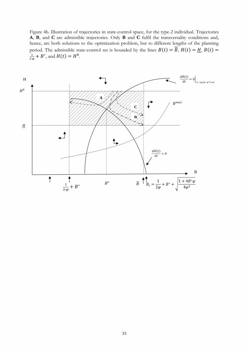
analyzed using modified versions of Figure 4a. For the type-2 individual, similar conclusions can
be drawn, using Figure 4b. Trajectories B and C are solutions to (6) for different planning
16
horizons, while trajectory A does not meet the transversality condition. For the type-2 individual,
any control starting point, , which is at a level lower than the equilibrium level, , is
inconsistent with the transversality condition and, hence, cannot be a solution to (6).
In more detail, trajectories that are consistent with the transversality condition are
depicted by setting in (9):
( )
, which gives
. Thus, as time approaches the planning horizon, the level of the
type 1 (2) -behaviour approaches ( .
4. DISCUSSION
By introducing – into the theoretical framework of the demand-for-health model – a non-
monotonic influence of health-related behaviour on health as well as punishments with respect to
health for deviations from a certain given activity level, , we were able to identify three types of
individuals and one unique equilibrium for each type, using the relation between the exerted level
of the health-related behaviour and . The effect on the equilibrium location of changes in
exogenous parameters, in particular, the rate at which any deviation from is “punished”, was
analysed. The qualitative properties of trajectories fulfilling both optimality and transversality
conditions were illustrated in a series of phase diagrams. The relationship between the location of
equilibria and the set of state-control trajectories that may solve the dynamic optimization
problem faced by the individual was analysed.
The phase diagram for the type-1 individual, Figure 4a, illustrates two possible solutions in the
control-state space, and one trajectory that does not fulfil the transversality condition which
implies that either or . It is clear from Figure 4a, that the location of the
isoclines in relation to both initial health and end-point health, determines the location of
17
potential solution trajectories. Moreover, individual preferences for the -behaviour play a
critical role – the stronger the preferences for , the further to the right is the vertical line
, and the smaller is the set of admissible optimal trajectories. At the point where
, the type-1 individual cannot identify any control-state trajectory that meets both
optimality and transversality conditions. Directly analogous conclusions can be drawn for the
type-2 individual's optimal choices. Thus, one fundamental implication of the model is that there
is not a continuous range of admissible values. Instead, the type-1 and type-2 individuals
will choose initial -behaviours within separate sets of values.
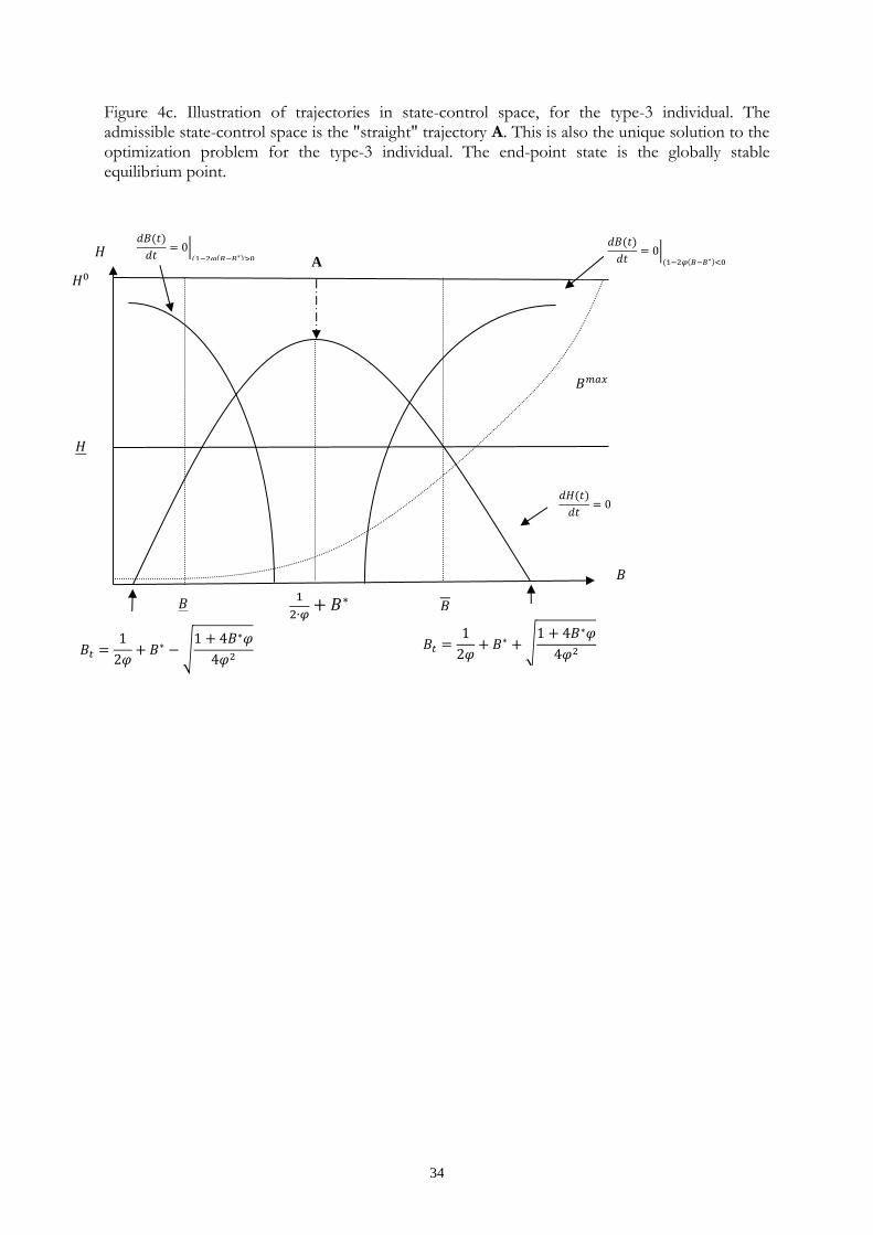
The type-3 individual is characterised by choosing exactly the physiological optimal level of at
all times. The optimal trajectory is vertical and goes from to the equilibrium amount of health
capital. Thus, if the type-3 individual starts at a health level above the equilibrium level, health
will decrease at the optimal trajectory. Notice, that the transversality condition is satisfied for the
type-3 individual in steady state:
, which is fulfilled, since, by
definition, for
, (
)
.
The model developed in this paper is very rich in that it extends the reach of the theoretical
toolbox for the analysis of a broad range of individual health and health-related behaviours, by
taking into account that several behaviours may be non-monotonically related to health. We will
illustrate the usefulness of the model by applying it to two specific issues: (1) the rate of
behaviour-specific atrophy and (2) the somewhat extended role that time preferences play when
non-monotonic effects are taken into account.
The fundamental notion behind this extended version of the demand-for-health model is that the
relationship between health benefits produced by a specific behaviour and the activity level of
18
that behaviour may show an inverted U-shape. The steepness of the function that connects the
level of behaviour and the resulting health effects reflects the rate at which the benefits diminish,
when the individual exert more or less than the level where there is no atrophy. So, what
conclusions can be drawn regarding individual decisions to partake in non-monotonic health
behaviours that differ regarding this rate ( )? First, the shape of the isoclines and the position of
the corresponding equilibrium differ between behaviours characterised by different 's. This is so
for all three types of individual. Second, different locations of isoclines and equilibrium mean that
both the admissible state-control set and the set of trajectories that are potential solutions to
problem (6) also differ between behaviours. The location of equilibrium in state-control space is
determined (partly) by the size of - see Claim 1. The difference between behaviours is also
reflected by the relative position of the isoclines, since any change in the location of an isocline
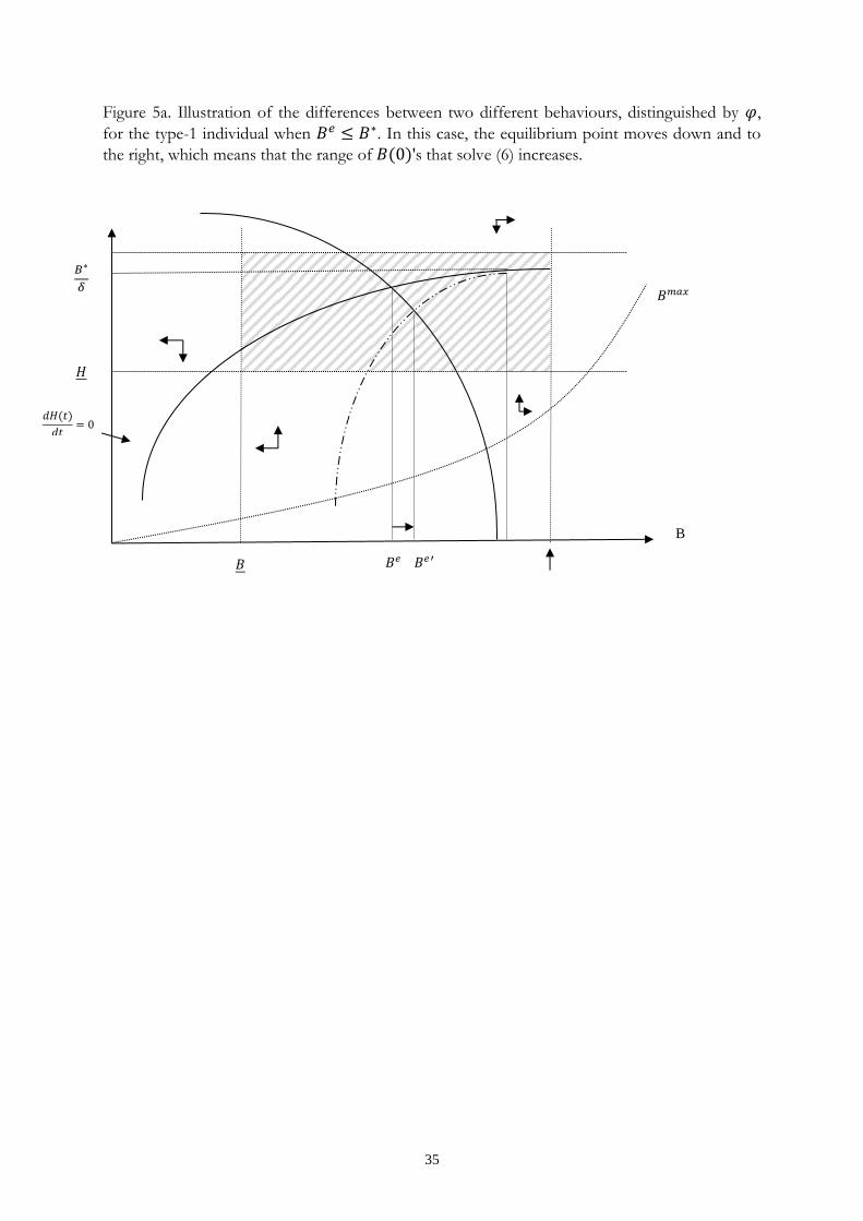
will alter the partition of the state-control space in behavioural sub-regions. Figure 5 illustrates
the difference between two different behaviours characterised by and , , for the type-
1 individual in the case when . This means that the equilibrium corresponding to
will lie to the south-east of the equilibrium point in the case. The -isocline will shift
according the illustration in Figure 2, around the point (
). The shift in the -isocline is
indeterminate, although some shifts can be ruled out based on Claim 1.
Figure 5 about here
The influence of time preferences differs between the type-1 and the type-2 individual. For both
types, the equilibrium level of health capital would decrease, while the equilibrium level of the -
behaviour would decrease for the type-1 and increase for the type-2 individual, if the future was
discounted heavier. Thus, as is clear from Figure 4, for the type-1 individual would move
closer to , which means that the range of -behaviours that are consistent with both optimality
19
and transversality conditions would shrink. Likewise, for the type-2 individual would move
closer to , which would reduce the set of potentially optimal trajectories. Differences in time
preferences are often suggested as a contributor to the different levels of investment in human
capital that are observed – the more farsighted individuals, the more investments in health and,
hence, the more advantageous is the level of public health. Our analysis demonstrates that this
conclusion is valid also for behaviours which have a non-monotonic influence on health.
The preceding analysis implies that, in general, health-related public policy has to take into
account that many behaviours may not be consistently bad or good for one’s health but rather
that the beneficial or detrimental effects depend on the individually chosen activity level of the
behaviour in question. Thus, a first-best health policy would distinguish between individuals who
exert low amounts and individuals who exert high amounts of a specific health-related behaviour.
An illustrative and, perhaps, provocative, example is alcohol consumption. Given that there is a
physiologically optimal level (strictly greater than zero) of alcohol consumption, taxing
individuals that consume above a certain threshold level, and maybe subsidizing those who
consume below the threshold, would increase population health, ceteris paribus. Obviously, the
same qualitative conclusion can be made concerning all health-related behaviours that may
influence health both positively and negatively. Thus, in order to affect such behaviours in a
health-promoting way, policy-makers would, in principle, have to incorporate not only
knowledge about the relationship between health and the target behaviour, but also a mechanism
that is dependent on the type of individual that will be affected. The lesson for policy-makers is
to rely less on general public-health policies and more on tailor-made measures for specific target
groups.

20
APPENDIX
Begin by noticing that along the -stationary locus, we have (take the time-derivative
of (9)). Then, we need to establish the sign of ’s partial derivatives, using
, and
( ) :
;
;
( )
–
( ) ;
( )
– ( )
(
– ) ( )
( ) , since (
– )
( ) .
Notice, that but ( ) .
The steady state loci
The
loci
In order to obtain the
loci, notice that implies that:
( ) . When ( ) , the implicit function
theorem yields:
( )
( )
( )
( )
In order to infer the curvature of the
loci, take the implicit derivative of
, which is
(leaving out arguments for brevity):
(
) (
)
,11
which means that the
- locus is decreasing in the left branch, and increasing in the right, and
concave. In the case when ( ) the locus is the vertical line at
. The shape of the the
locus, combined with the previously shown
11 .

21
shape of the
locus, establish that there is one unique steady-state point for each
individual type.
Comparative statics – type 1 and 2
For a change in a parameter, , the effects on steady-state levels of health capital and the -
behaviour, and , can be obtained by applying Cramer’s rule to the following system
(arguments left out). Notice, in steady state, ( ),
( ), and ( ). For the type-1 and 2
individuals we have:
(
) (
) (
).
(
) is the Jacobian matrix of equations (9) and (11) evaluated in steady state.
Applying Cramer’s rule in the case of a change in , we have: (
)
(
|
|
| |
|
|
| |
)
.
The sign of | |
| | | ( )
( ) ( )|
Since ( ) , the determinant is always negative.
The steady state effects of
Applying Cramer’s rule to the equations system above gives, for :
( )
| |
( ) ( )
| |
( ) ( )
( ) ( )
| |
( )
| |
In order to see that
, use the second term in , and reformulate the second term in
the ratio above to get the condition for
:

22
( )
( ) . When this reduces to the condition
,
which will always be fulfilled when
. For
, the conclusion follows
immediately. For , notice that
(follows from (9)), which makes the
numerator is positive. When , the numerator is 0.
For , we have:
( )
| |
( )
| |,
which is if , and if , and when .
The sign is indeterminate when
, due to the second term in the numerator.
Steady state effects of
Applying Cramer’s rule the equations system above (substituting for ), gives:
| | ( ) if .
| | .
Steady state effects of
First, . Then, again applying Cramer’s rule to the equations system above ( has
been substituted for ):
( ) ( )
| |
( ) ( )
| |
Steady state effects of E
Proceeding as before gives:

23
| | ( ) if , and
.
| | if .
Steady state effects of
First, . Then, again applying Cramer’s rule to the equations system above gives:
( )
| |
( )
| | if .
Comparative statics – type 1 and 2
For the type-3 individual, a change in the parameter , we have:
, except for .
Thus, the change in is given by (10) and
:
and
.
Summary of comparative statics results
Table A1. Comparative static results regarding steady-state levels of health and the -behaviour. We assume that
the effect of knowledge, E, on the one-unit cost, , is negative. If the effect had been positive the results in the third raw would be reversed.
Type 1
Type 2
Type 3
, , , ,0
, , , 0,0
, , , ,0
, , , 0,0
, , 0,0

24
Equilibrium properties
The cases when
The terms of the Jacobian matrix J are obtained from
( )
( )
. Taking the derivative with respect to gives:
( ( ))
. Similarly, taking the derivative of G with respect
to yields:
( ( ))
. For a steady state we have:
( ( ))
.
Together with and we are able to formulate:
| | ( ( ))
( ( ) )
.
| | is a necessary and sufficient condition for a saddle point and, hence, the result follows.
The cases when
In this case the determinant of the Jacobian matrix is zero, and the trace is strictly negative, i.e.,
one eigenvalue is zero and the other is strictly negative. This implies a sink.
25
REFERENCES
Asano, T., Shibata, A., 2011. Risk and uncertainty in health investment. European Journal of Health Economics 12:79-85. Becker, G.S., Murphy, K.S., 1988. A theory of rational addiction. Journal of Political Economy 96:675-700. Bize, R., Johnson, J.A., Plotnikoff, R.C., 2007. Physical activity level and health-related quality of life in the general adult population: A systematic review. Preventive Medicine 45:401-415. Bolin, K., Jacobson, L., Lindgren, B., 2001. The family as the producer of health – when spouses are Nash bargainers. Journal of Health Economics 20:349-362. Bolin, K., Jacobson, L., Lindgren, B., 2002a. The demand for health and health investments in Sweden 1980/81, 1990/91 and 1996/97. In: Lindgren, B. (Ed.) Individual Decisions for Health. Routledge, London, 93-112. Bolin, K., Jacobson, L., Lindgren, B., 2002b. The family as the producer of health – when spouses act strategically. Journal of Health Economics 21: 475-495. Bolin, K., Jacobson, L., Lindgren, B., 2002c. Employer investments in employee health - Implications for the family as health producer. Journal of Health Economics 21:563-583. Bolin, K., Lindgren, B., Lindström, M., Nystedt, P., 2003. Investments in social capital – implications of social interactions for the production of health. Social Science & Medicine 56:2379-2390. Buxton, O.M., Marcelli, E., 2010. Short and long sleep are positively associated with obesity, diabetes, hypertension, and cardiovascular disease among adults in the United States. Social Science & Medicine 71:1027-1036. Caputo, M.R., 2005. Foundations of Dynamic Economic Analysis – Optimal Control Theory and Applications. Cambridge University Press, Cambridge. Chang, F., 1996. Uncertainty and investment in health. Journal of Health Economics 15: 369-376. Chang, Y.M., 2009. Strategic altruistic transfers and rent seeking within the family. Journal of Population Economics 22:1081-1098. Chang, Y.M., Weisman, D.L., 2005. Sibling rivalry and strategic parental transfers. Southern Economic Journal 71(4):821-836. Chiang, A.C., 1992. Elements of Dynamic Optimization. McGraw Hill, Singapore. Colditz, G.A., 1999. Economic costs of obesity and inactivity. Medicine and Science in Sports and Exercise 31:S663-667. Colditz, G.A., 2000. Illnesses caused by smoking cigarettes. Cancer Causes and Control 11:93-97.

26
Cutler, D.M., Gleaser, E., 2005. What explains differences in smoking, drinking, and other health-related behaviours. American Economic Review 95(2):238-242. Dal Grande, E., Gill, T., Wyatt, L., Chittleborough, C.R., Phillips, P.J., Taylor, A.W., 2009. Population attributable risk (PAR) of overweight and obesity on chronic diseases: South Australian representative, cross-sectional data, 2004-2006. Obesity Research & Clinical Practice 3:159-168. Dardanoni, V., Wagstaff, A., 1987. Uncertainty, inequalities in health and the demand for health. Journal of Health Economics 6:283-290. Dardanoni, V., Wagstaff, A., 1990. Uncertainty and the demand for medical care. Journal of Health Economics 9:23-38. Dockner, J.E., Feichtinger, G., 1993. Cyclical consumption patterns and rational addiction. American Economic Review 83(1):256-263. Doll, R., Peto, R., 1976. Mortality in relation to smoking: 20 years’ observations on male British doctors. British Medical Journal 2:1525-1536. Doll, R., Peto, R., Wheatley, K., Gray, R., Sutherland, I., 1994. Mortality in relation to smoking: 40 years’ observations on male British doctors. British Medical Journal 309:901-911. Ehrlich, I., 2000. Uncertain lifetime, life protection, and the value of life saving. Journal of Health Economics 19:341-367. Ehrlich, I., 2001. Erratum to “ Uncertain lifetime, life protection, and the value of life saving”. Journal of Health Economics 20:459-460. Ehrlich, I., Chuma, H., 1990. A model of the demand for longevity and the value of life extensions. Journal of Political Economy 98:761-782. Forster, M., 2001. The meaning of death: some simulations of a model of healthy and unhealthy consumption. Journal of Health Economics 20:613-638. Galama, T., 2011. A contribution to health capital theory. Working Paper WR-831. Rand Corporation, Santa Monica, CA. Galama, T., Kapteyn A., 2011. Grossman’s missing health threshold. Journal of Health Economics 30:1044-1056. Garrett, N.A., Brasure, M., Schmitz, K.H., Schultz, M.M., Huber, M.M., 2004. Physical inactivity. Direct cost to a health plan. American Journal of Preventive Medicine 27:304-309. Grossman, M., 1972a. The Demand for Health: A Theoretical and Empirical Investigation, Columbia University Press for the National Bureau of Economic Research. Grossman, M., 1972b. On the concept of health capital and the demand for health. Journal of Political Economy 80:223 – 255.
27
Grossman, M., 2000. The human capital model of the demand for health. In: Culyer, A.J., Newhouse, J.P. (Eds.). Handbook of Health Economics. Elsevier, Amsterdam, 347-408. Grönbaeck, M., 2009. The positive and negative health effects of alcohol – and the public health implications. Journal of Internal Medicine 265:407-420. Grönbaeck, M., Deis, A., Becker, U., Hein, H.O., Schnohr, P., Jensen, G., Borch-Johnsen, K., Sörensen, T.I.A., 1998. Alcohol and mortality: is there a U-shaped relation in elderly people? Age and Ageing 27:739-744. Howatson, G., van Someren, K.A., 2008. The prevention and treatment of exercise-induced muscle damage. Sports Medicine 38:483-503. Jacobson, L., 2000. The family as producer of health – An extension of the Grossman model. Journal of Health Economics 19:611-637. Ji, L.L., 2001. Exercise at old age: Does it increase or alleviate oxidative stress? Annals of the New York Academy of Sciences 928:236-247. Kenkel, D.S., 1991. Health behaviour, health knowledge, and schooling. Journal of Political Economy 99: 287-305. Kenkel, D.S., 2000. Prevention. In: Culyer, A.J., Newhouse, J.P. (Eds.). Handbook of Health Economics. Elsevier, Amsterdam, 1675-1720. Knuth, A.G., Hallai, P.C., 2009. Temporal trends in physical activity: A systematic review. Journal of Physical Activity and Health 6:548-559. Liljas, B., 1998. The demand for health with uncertainty and insurance. Journal of Health Economics 17:153-170. Liljas, B., 2000. Insurance and imperfect financial markets in Grossman’s demand for health model - a reply to Tabata and Ohkusa. Journal of Health Economics 19: 811-820. Liljas, B., 2002. An exploratory study on the demand for health, life-time income, and imperfect financial markets. In: Lindgren, B. (Ed.) Individual Decisions for Health. Routledge, London, 29-40. Locke, S., 1999. Exercise-related chronic lower leg pain. Australian Family Physician 28:569-573. Morton, J.P., Kayani, A.C., McArdle, A,, Drust, B., 2009. The exercise-induced stress response of skeletal muscle, with specific emphasis on humans. Sports Medicine 39:643-662. Must, A., Spadano, J., Coakley, E.H., Field, A.E., Colditz, G., Dietz, W.H., 1999. The disease burden associated with overweight and obesity. JAMA 282:1523-1529. Muurinen, J.M., 1982. Demand for health. A generalised Grossman model. Journal of Health Economics 1:5-28.
28
Picone, G., Uribe, M., Wilson, M.R., 1998. The effect of uncertainty on the demand for medical care, health capital and wealth. Journal of Health Economics 17:171-185. Randolph, C., 2008. Exercise-induced bronchospasm in children. Clinical Review of Allergy and Immunology 34:205-216. Sabanayagam, C., Shankar, A., 2010. Sleep duration and cardiovascular disease: Results from the National Health Interview Survey. SLEEP 33:1037-1042. Steinhausen, H.C., 2002. The outcome of anorexia nervosa in the 20th century. American Journal of Psychiatry 159:1284-1293. Steinhausen, H.C., Weber, S., 2009. The outcome of bulimia nervosa: Findings from one-quarter century of research. American Journal of Psychiatry 166:1331-1341. Swedish National Food Agency. www.slv.se. 2012. Tisi, P.V., Shearman, C.P., 1998. The evidence for exercise-induced inflammation in intermittent claudication: Should we encourage patients to stop walking? European Journal of Vascular and Endovascular Surgery 15:7-17. Vineis, P., Alavanja, M., Buffler, P., Fibtgan, E., Franceschi, S., Gao, T., Gupta, P.C., Hackshaw, A., Matos, E., Samet, J., Sitas F, Smith J, Stayner L, Straif K, Thun MJ, Wichmann HE, Wu AH, Zaridze D, Peto R, Doll R. Tobacco and cancer: Recent epidemiological evidence. Journal of the National Cancer Institute 96:99-106.
29
Figure 1. Relative risk of mortality in realtion to alcohol intake for middle-aged (-) and elderly (.....) people. Risk was set att 1.00 at lowest mortality at 1-6 beverages per week. Vertical lines are 95% confidence intervals for point depicting estimates for all subjects. Reproduced from Grönbaeck et al. (1998) with permission of the Oxford University Press.
30
Figure 2. Illustration of the relationship between behaviour, B, and the amount of health
investment, I. The parabola is the graph of the function . The maximum influence on health attainable through the behaviour, B, is at the inflexion point of the
parabola. The solid-line parabola corresponds to the value , while the high-location dotted
parabola corresponds to the value , and the low-location dotted parabola corresponds to
the value .
B
I
√
√
31
Figure 3. Illustration of stationary loci, and admissible sets, for the control- and state variable.
Equilibrium points are marked with a dot. The parabola shows the
locus, the
hyperbolas the
locus. The filled rectangle marks the admissible state-control set for the
type 1 individual. The dotted curve, , marks the maximum affordable level of for each amount of health capital. Since we have assumed that less than the maximum affordable level of
is always demanded by all types, this curve is drawn below the admissible control sets.
|
|
√
√
|
Type 1 Type 2
32
Figure 4a. Illustration of trajectories in state-control space, for the type-1 individual. Trajectories A, B, and C are admissible trajectories. Only A and B fulfil the transversality conditions and, hence, are both solutions to the optimization problem, but to different lengths of the planning
period. The admissible state-control set is bounded by the lines , ,
, and .
B
H
|
√
A B C
33
Figure 4b. Illustration of trajectories in state-control space, for the type-2 individual. Trajectories A, B, and C are admissible trajectories. Only B and C fulfil the transversality conditions and, hence, are both solutions to the optimization problem, but to different lengths of the planning
period. The admissible state-control set is bounded by the lines , ,
, and .
B
H
|
√
○
A
B
C
34
Figure 4c. Illustration of trajectories in state-control space, for the type-3 individual. The admissible state-control space is the "straight" trajectory A. This is also the unique solution to the optimization problem for the type-3 individual. The end-point state is the globally stable equilibrium point.
|
|
√
√
A
35
Figure 5a. Illustration of the differences between two different behaviours, distinguished by ,
for the type-1 individual when . In this case, the equilibrium point moves down and to
the right, which means that the range of 's that solve (6) increases.
B