Non-Linear Relationships - Section 5cathy/Math2311/Lectures/Spring 18/lecture15c.pdf · the population int he city of Houston from 1900 to 2010. Year Population 1900 44,633 1910 78,800

Non-Linear RelationshipsSection 5.4

Cathy Poliak, [email protected] in Fleming 11c

Department of MathematicsUniversity of Houston

Lecture 14 - 2311

Cathy Poliak, Ph.D. [email protected] Office in Fleming 11c (Department of Mathematics University of Houston )Section 5.4 Lecture 14 - 2311 1 / 24

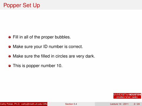
Popper Set Up

Fill in all of the proper bubbles.

Make sure your ID number is correct.

Make sure the filled in circles are very dark.

This is popper number 10.


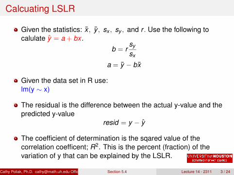
Calcuating LSLR

Given the statistics: x , y , sx , sy , and r . Use the following tocalulate y = a + bx .

b = rsy

sx

a = y − bx

Given the data set in R use:lm(y ∼ x)

The residual is the difference between the actual y-value and thepredicted y-value

resid = y − y

The coefficient of determination is the sqared value of thecorrelation coefficent; R2. This is the percent (fraction) of thevariation of y that can be explained by the LSLR.


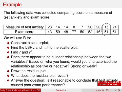
Example

The following data was collected comparing score on a measure oftest anxiety and exam score:

Measure of test anxiety 23 14 14 0 7 20 20 15 21Exam score 43 59 48 77 50 52 46 51 51

We will use R to:Construct a scatterplot.Find the LSRL and fit it to the scatterplot.Find r and r2.Does there appear to be a linear relationship between the twovariables? Based on wha you found, would you characterized therelationship as positive or negative? Strong or weak?Draw the residual plot.What does the residual plot reveal?Answer the question: Is it reasonable to conclude that test anxietycaused poor exam performance?



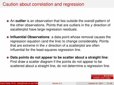
Caution about correlation and regression

An outlier is an observation that lies outside the overall pattern ofthe other observations. Points that are outliers in the y direction ofsacatterplot have large regression residuals.

Influential Observations: a data point whose removal causes theregression equation (and the line) to change considerably. Pointsthat are extreme in the x direction of a scatterplot are ofteninfluential for the least-squares regression line.

Data points do not appear to be scatter about a straight line:First draw a scatter diagram if the points do not appear to bescattered about a straight line, do not determine a regression line.


Caution about correlation and regression

Extrapolation: Using the regression equation to make predictionsfor values of the predictor variable outside the range of theobserved values of the predictor variable. (Grossly incorrectpredictions can result from extrapolation.)

Lurking Variable: A variable that is not among the explanatory orresponse variables in a study and yet may influence theinterpretation of relationships among those variables.

Association does not imply causation.


Popper 10 Questions

The following are the statistics to calculate a least squares line (LSLR)to predict the final grade (score) by the average quiz score. Score:mean = 71.09433, sd = 28.0842; Quiz: mean = 71.17697, sd =25.87901; Correlation: r = 0.93257

1. Determine the LSLR to predict the final score based on the quizscore.

a. y = −0.939326 + 1.012x b. y = 10.0826 + 0.8593xc. y = 70.913 d. y = 1 + 0.85x

2. A person has a quiz average for the semester at 86, has a finalscore of 93. Determine the residual for this student.

a. 6.9 b. 86.1 c. -6.9 d. 03. Determine the coefficient of determination.

a. 0.93257 b. 0.8967 c. 0.9215 d. 1.0852


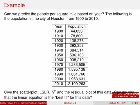
ExampleCan we predict the people per square mile based on year? The following isthe population int he city of Houston from 1900 to 2010.

Year Population1900 44,6331910 78,8001920 138,2761930 292,3521940 384,5141950 596,1631960 938,2191970 1,233,5051980 1,595,1381990 1,631,7662000 1,953,6312010 2,100,263

Give the scatterplot, LSLR, R2 and the residual plot of this data. Can we saythat the linear equation is the "best fit" for this data?


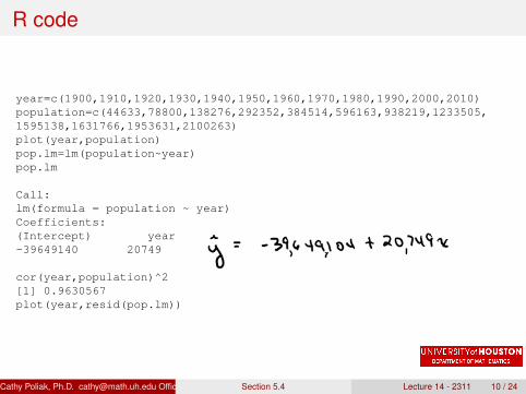
R code

year=c(1900,1910,1920,1930,1940,1950,1960,1970,1980,1990,2000,2010)population=c(44633,78800,138276,292352,384514,596163,938219,1233505,1595138,1631766,1953631,2100263)plot(year,population)pop.lm=lm(population~year)pop.lm

Call:lm(formula = population ~ year)Coefficients:(Intercept) year-39649140 20749

cor(year,population)^2[1] 0.9630567plot(year,resid(pop.lm))


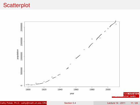
Scatterplot

1900 1920 1940 1960 1980 2000

050

0000

1000

000

1500

000

2000

000

year

popu

latio

n


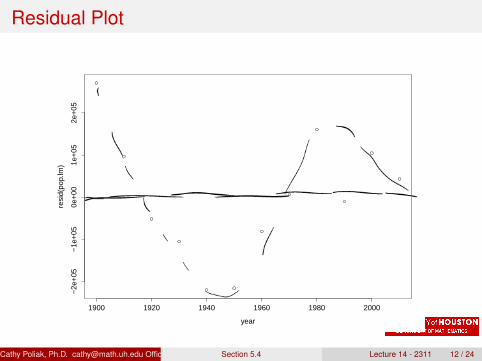
Residual Plot

1900 1920 1940 1960 1980 2000

−2e

+05

−1e

+05

0e+

001e

+05

2e+

05

year

resi

d(po

p.lm

)


Results

The coefficient of determination, R2 is high.

The scatter plot and residual plot shows a non-linear pattern.

The least-square regression line might not be the "best fit" for thisdata.


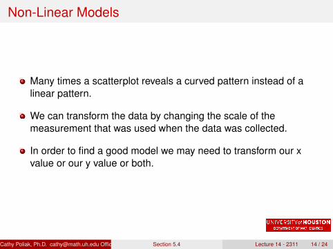
Non-Linear Models

Many times a scatterplot reveals a curved pattern instead of alinear pattern.

We can transform the data by changing the scale of themeasurement that was used when the data was collected.

In order to find a good model we may need to transform our xvalue or our y value or both.


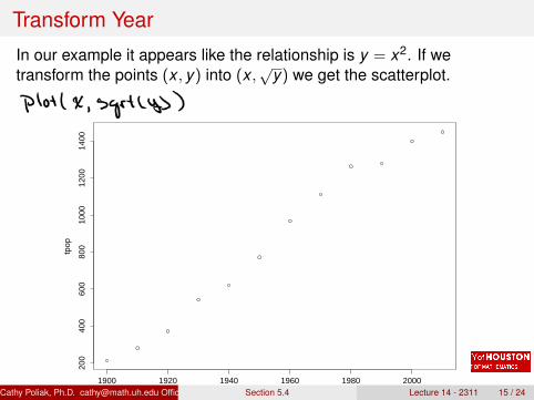
Transform Year

In our example it appears like the relationship is y = x2. If wetransform the points (x , y) into (x ,

√y) we get the scatterplot.

1900 1920 1940 1960 1980 2000

200

400

600

800

1000

1200

1400

year

tpop


R code

tpop=sqrt(population)plot(year,tpop)tpop.lm=lm(tpop~year)tpop.lm

Call:lm(formula = tpop ~ year)Coefficients:(Intercept) year-23267.19 12.34

cor(year,tpop)^2[1] 0.9854597plot(year,resid(tpop.lm))lines(year,rep(0,length(year)))


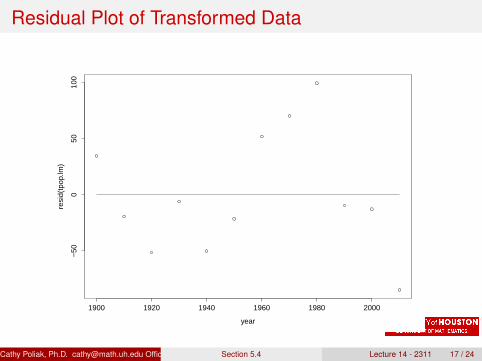
Residual Plot of Transformed Data

1900 1920 1940 1960 1980 2000

−50

050

100

year

resi

d(tp

op.lm

)


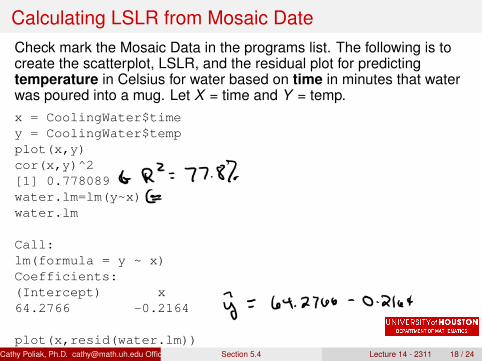
Calculating LSLR from Mosaic DateCheck mark the Mosaic Data in the programs list. The following is tocreate the scatterplot, LSLR, and the residual plot for predictingtemperature in Celsius for water based on time in minutes that waterwas poured into a mug. Let X = time and Y = temp.x = CoolingWater$timey = CoolingWater$tempplot(x,y)cor(x,y)^2[1] 0.778089water.lm=lm(y~x)water.lm

Call:lm(formula = y ~ x)Coefficients:(Intercept) x64.2766 -0.2164

plot(x,resid(water.lm))Cathy Poliak, Ph.D. [email protected] Office in Fleming 11c (Department of Mathematics University of Houston )Section 5.4 Lecture 14 - 2311 18 / 24

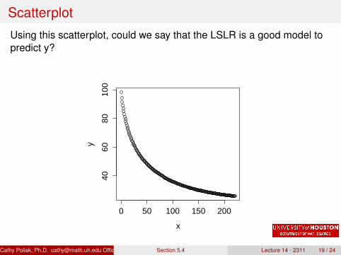
Scatterplot

Using this scatterplot, could we say that the LSLR is a good model topredict y?

0 50 100 150 200

4060

8010

0

x

y


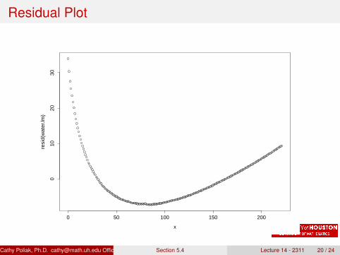
Residual Plot

0 50 100 150 200

010

2030

x

resi

d(w

ater

.lm)


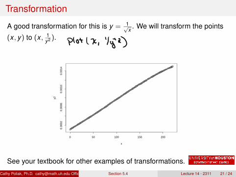
Transformation

A good transformation for this is y = 1√x . We will transform the points

(x , y) to (x , 1y2 ).

0 50 100 150 200

0.00

020.

0006

0.00

100.

0014

x

y2

See your textbook for other examples of transformations.


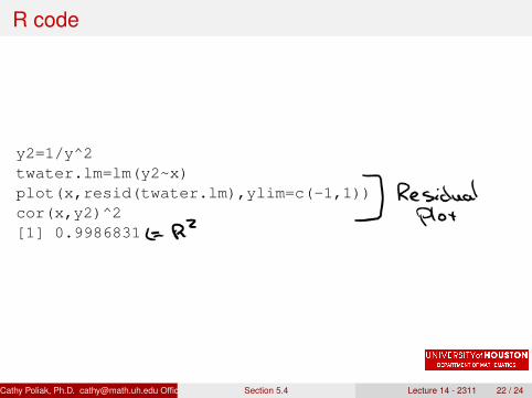
R code

y2=1/y^2twater.lm=lm(y2~x)plot(x,resid(twater.lm),ylim=c(-1,1))cor(x,y2)^2[1] 0.9986831


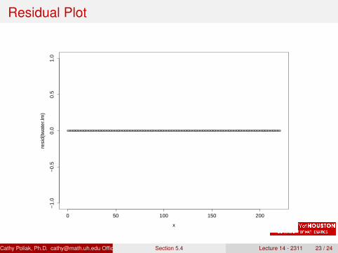
Residual Plot

0 50 100 150 200

−1.

0−

0.5

0.0

0.5

1.0

x

resi

d(tw

ater

.lm)


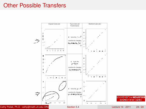
Other Possible Transfers

Original Scatter-plot Type of plot and Transformation

Modified Scatter-plot

looks like

transform by changing

looks like


looks like



Documents

Non-Linear Relationships - Section 5cathy/Math2311/Lectures/Spring 18/lecture15c.pdf · the population int he city of Houston from 1900 to 2010. Year Population 1900 44,633 1910 78,800