Rail Safety IDEA Program

Non-contact Deflection Monitoring System for Timber Railroad Bridges

Final Report for Rail Safety IDEA Project 35 Prepared by: Sudhagar Nagarajan, Florida Atlantic University M. Arockiasamy, Florida Atlantic University Bill Spencer, Jr., University of Illinois Urbana-Champaign March 2019

Innovations Deserving Exploratory Analysis (IDEA) Programs Managed by the Transportation Research Board

This IDEA project was funded by the Rail Safety IDEA Program.

The TRB currently manages the following three IDEA programs:

• The NCHRP IDEA Program, which focuses on advances in the design, construction, and maintenance of highway systems, is funded by American Association of State Highway and Transportation Officials (AASHTO) as part of the National Cooperative Highway Research Program (NCHRP).

• The Rail Safety IDEA Program currently focuses on innovative approaches for improving railroad safety or performance. The program is currently funded by the Federal Railroad Administration (FRA). The program was previously jointly funded by the Federal Motor Carrier Safety Administration (FMCSA) and the FRA.

• The Transit IDEA Program, which supports development and testing of innovative concepts and methods for advancing transit practice, is funded by the Federal Transit Administration (FTA) as part of the Transit Cooperative Research Program (TCRP).

Management of the three IDEA programs is coordinated to promote the development and testing of innovative concepts, methods, and technologies.

For information on the IDEA programs, check the IDEA website (www.trb.org/idea). For questions, contact the IDEA programs office by telephone at (202) 334-3310.

IDEA Programs Transportation Research Board 500 Fifth Street, NW Washington, DC 20001

The project that is the subject of this contractor-authored report was a part of the Innovations Deserving Exploratory Analysis (IDEA) Programs, which are managed by the Transportation Research Board (TRB) with the approval of the National Academies of Sciences, Engineering, and Medicine. The members of the oversight committee that monitored the project and reviewed the report were chosen for their special competencies and with regard for appropriate balance. The views expressed in this report are those of the contractor who conducted the investigation documented in this report and do not necessarily reflect those of the Transportation Research Board; the National Academies of Sciences, Engineering, and Medicine; or the sponsors of the IDEA Programs.

The Transportation Research Board; the National Academies of Sciences, Engineering, and Medicine; and the organizations that sponsor the IDEA Programs do not endorse products or manufacturers. Trade or manufacturers’ names appear herein solely because they are considered essential to the object of the investigation.

RAIL SAFETY IDEA PROGRAM COMMITTEE

CHAIR CONRAD RUPPERT, JR. Railway Engineering Educator &Consultant

MEMBERS TOM BARTLETT Transportation Product Sales Company MELVIN CLARK LTK Engineering Services MICHAEL FRANKE Retired Amtrak BRAD KERCHOF Norfolk Southern Railway MARTITA MULLEN Canadian National Railway STEPHEN M. POPKIN Volpe National Transportation Systems Center

FRA LIAISON TAREK OMAR Federal Railroad Administration

TRB LIAISON SCOTT BABCOCK Transportation Research Board

IDEA PROGRAMS STAFF GWEN CHISHOLM-SMITH, Manager, Transit Cooperative Research Program VELVET BASEMERA-FITZPATRICK, Senior Program Officer DEMISHA WILLIAMS, Senior Program Assistant

EXPERT REVIEW PANEL SAFETY IDEA PROJECT 35 MELVIN CLARK, LTK Engineering Services MAURICE ELLIOT, Florida Department of Transportation CHRISTOPHER MOALE, CSX Transportation Inc. DUANE OTTER, Transportation Technology Center, Inc.

Non-contact Deflection Monitoring System for Timber Railroad Bridges

IDEA Program Final Report For the period July 2017 through March 2019

Contract Number: Rail Safety 35

Prepared for the IDEA Program Transportation Research Board

National Research Council

Sudhagar Nagarajan, Ph.D. Assistant

Professor

Civil, Environmental and Geomatics Engineering

Florida Atlantic University

M. Arockiasamy, Ph.D., P.E., P.Eng., Fellow ASCE

Professor

Civil, Environmental and Geomatics Engineering

Florida Atlantic University

Bill Spencer, Jr., Ph.D.

Professor

University of Illinois Urbana-Champaign

Submittal Date March 31, 2019

ACKNOWLEDGMENTS

This project was supported by the National Academies of Sciences, Engineering and Medicine, Transportation Research Board’s Rail Safety IDEA Program.

The investigators of the project would like to thank the Oversight Committee, IDEA Program Manager Dr. Velvet Basemera-Fitzpatrick and former IDEA Program Manager Ms. Jo Allen Gause for the guidance, feedback and support during all stages of the project.

The project team would like to express their sincere gratitude to the following Expert Review Panel members who spent several hours of their precious time in reviewing the project reports and attending the quarterly web conferences. Their participation significantly contributed to the project.

• Mr. Melvin Clark, LTK Engineering Services (Rail Safety IDEA Oversight Committee Liaison)

• Mr. Maurice Elliot, Florida Department of Transportation

• Mr. Christopher Moale, CSX Transportation Inc.

• Dr. Duane Otter, Transportation Technology Center, Inc.

The investigators would like to thank CSX Transportation for dedicating their resources to the project by meeting with us and providing access to their timber railroad bridges in South Florida. Among several CSX engineers who helped with the project, the investigators would like to specifically thank Christopher Moale, Terri Grey, Ed Sparks and Jon Hirst who were in the frontline.

The project team also would like to thank the students who relentlessly worked hard for the completion of this project. The contribution of following students is acknowledged.

• Ishwarya Srikanth (Ph.D. Candidate)

• Satarupa Khamaru (M.S Student)

• Stephen Castillo (M.S Student)

• Gerardo Rojas (Undergraduate Student)

iii

TABLE OF CONTENTS ACKNOWLEDGMENTS .................................................................................................................................................... ii

List of Tables ........................................................................................................................................................................iv

List of Figures .......................................................................................................................................................................iv

Executive Summary ............................................................................................................................................................... 1

IDEA Product ........................................................................................................................................................................ 1

Concept and Innovation ......................................................................................................................................................... 1

Project Results ................................................................................................................................................................. 2

Product Payoff Potential .................................................................................................................................................. 2

Product Transfer ............................................................................................................................................................... 2

Investigation .......................................................................................................................................................................... 2

Current state of practice and limitations .......................................................................................................................... 2

Development of Deflection Monitoring System (DMS) .................................................................................................. 3

Selection of Camera for DMS .................................................................................................................................... 3

Selection of Terrestrial Laser Scanner for DMS ........................................................................................................ 4

Automated Linear Feature Extraction and Matching ....................................................................................................... 4

Line Segment Extraction from Image Data ................................................................................................................ 4

Linear feature extraction from Terrestrial Laser Scanning (TLS) Data ...................................................................... 5

Linear Feature Matching ............................................................................................................................................ 5

Implementation of linear feature-based image registration .............................................................................................. 6

Linear Feature-based Computation of EO .................................................................................................................. 6

Camera Calibration ..................................................................................................................................................... 6

Development of deflection measurement methodology using DMS ................................................................................ 7

Feature Tracking ......................................................................................................................................................... 7

2D Deflection Methodology ....................................................................................................................................... 8

3D Deflection Methodology ....................................................................................................................................... 8

Field Experiments .......................................................................................................................................................... 10

Field Test Setup ........................................................................................................................................................ 10

Non-Contact Deflection Results ............................................................................................................................... 13

Results from Deflectometer ...................................................................................................................................... 15

Finite Element Analysis ................................................................................................................................................. 17

Site 1: Three-span Open Deck Bridge at Valrico (SV849.90), Built in 1948 ........................................................... 17

Site 2: Six-span Ballasted Deck Bridge at Lorida (SX878.8), Built in 1955 ............................................................ 19

Effect on Stiffness (K) of the Stringer and Pile Due to the Presence of Imperfections/Cracks ................................ 20

Comparison of Results ................................................................................................................................................... 20

Plans for implementation ..................................................................................................................................................... 22

Conclusions ......................................................................................................................................................................... 22

Investigator Profile .............................................................................................................................................................. 23

iv

References ........................................................................................................................................................................... 23

LIST OF TABLES

TABLE 1. Material and Geometric Properties of Timber Trestle Bridge ........................................................................... 17 TABLE 2. Comparison of Deflection Measurements for Site 1 .......................................................................................... 21 TABLE 3. Comparison of Deflection Measurements for Site 2 .......................................................................................... 21

LIST OF FIGURES

FIGURE 1. Edges extracted from Canny algorithm overlaid on original grayscale image of bridge site 1: Three span timber trestle bridge - SV 849.90 (VL-Valrico) ................................................................................................................................ 5 FIGURE 2. Methodology flow-chart for exterior orientation computation ........................................................................... 7 FIGURE 3. Methodology to compute 2D deflection using a single camera with known EO ............................................... 8 FIGURE 4. Illustration of 2D deflection computation .......................................................................................................... 9 FIGURE 5. Methodology to compute 3D deflection using two cameras with known EO .................................................... 9 FIGURE 6. 3D Deflections are computed by intersecting projection rays from two images .............................................. 10 FIGURE 7. Field Test Set-up for Site SV 849.9 .................................................................................................................. 11 FIGURE 8. CSX 6 Axle-Locomotive (Freight Train) used for dynamic load testing in SV 849.9 ..................................... 11 FIGURE 9. Field Test Set-up for Site SX 878.8 .................................................................................................................. 11 FIGURE 10. Amtrak passenger car axles used for dynamic load testing in SX 878.8 ........................................................ 12 FIGURE 11. 3D Laser Scan of SV 849.9 Bridge ................................................................................................................ 12 FIGURE 12. 3D laser scan of SX 878.8 bridge ................................................................................................................... 12 FIGURE 13. SV 849.9 bridge lateral deflections derived from photogrammetry ............................................................... 13 FIGURE 14. SV 849.9 Bridge vertical deflections derived from photogrammetry ............................................................. 13 FIGURE 15: SV 849.9 Bridge vertical deflections derived from photogrammetry (Enlarged version) .............................. 14 FIGURE 16. SX 878.8 Bridge lateral deflections derived from photogrammetry ............................................................... 14 FIGURE 17. SX 878.8 Bridge vertical deflections derived from photogrammetry ............................................................. 15 FIGURE 18. SX 878.8 Bridge vertical deflections derived from photogrammetry (enlarged version) ............................... 15 FIGURE 19.Vertical displacement of stringer from deflectometer ..................................................................................... 16 FIGURE 20. Lateral displacement of pile/pile cap from deflectometer .............................................................................. 16 FIGURE 21. Vertical displacement of stringer from deflectometer .................................................................................... 16 FIGURE 22. 3D view of the analytical model ..................................................................................................................... 18 FIGURE 23. Axle load and spacing .................................................................................................................................... 18 FIGURE 24. Vertical deformation contour for stringer due to moving live load (silty or clayey fine to coarse sand- loose consistency) ......................................................................................................................................................................... 19 FIGURE 25. Standard 3-D view of the model in CSIBridge (left); Extruded 3-D view of the model (right) ..................... 19 FIGURE 26. Vertical deformation contour for stringer due to moving live load (for silty or clayey fine to coarse sand- loose consistency) ......................................................................................................................................................................... 20 FIGURE 27. As-is condition of the open deck bridge in Valrico; As-is condition of the ballasted-deck bridge in Lorida . 20

1

EXECUTIVE SUMMARY

This report summarizes the results of non-contact deflection monitoring system developed for timber railroad bridges. Considering the abundance of timber railroad bridges in the nation that have exceeded their design life, a cost-effective and safe deflection monitoring system is essential for their regular maintenance. As existing techniques typically require access to the bridge structure that poses safety challenges for the bridge maintenance crew, this project has developed a completely non-contact and low-cost bridge deflection monitoring system using cameras. The project demonstrated the feasibility of using camera as a bridge deflection measurement sensor by implementing the techniques in CSX-owned railroad bridges in South Florida. The project team carefully studied the characteristics of timber railroad bridges in the nation based on AREMA guidelines. Accordingly, the project team analyzed the suitable camera parameters to capture bridge deflections. The recommended parameters are discussed in the report. In order to scale the images captured by cameras, the project methodology adopted laser scanner or total station and a linear feature- based registration technique. With the single camera, 2D deflections can be recovered. When two or more cameras are used, 3D deflections can be derived using the demonstrated project methodology. The project team developed necessary mathematical models and workflow to derive 2D/3D deflections from the images acquired by cameras.

The project investigators demonstrated the feasibility of the developed methodology in both lab environment and the field conditions. As for field testing of project methodology, the investigators worked with CSX Transportation and selected several candidate bridges and used two of them. The image sequences (video) captured by the camera were used to automatically track the deflection of specific points of interest when a dynamic load was applied. The derived results were compared with dial gages and finite element analysis for validation.

IDEA PRODUCT

This project developed an innovative non-contact linear feature-based deflection measurement system using Terrestrial Laser Scanning (TLS) and cameras for timber railroad bridges. The requirement of control points to register images was circumvented by using the 3D model of the bridge created in dead load condition by TLS. This research project developed a rigorous linear feature-based registration mathematical model to determine the orientation of images, so they can be used to derive 2D/3D deflections under different static and live load conditions. Though this research mainly focused on timber railroad bridges, it can be applied to other steel and masonry railroad bridges. The project i) developed a Deflection Monitoring System (DMS) that includes a camera ii) developed a linear feature-based registration methodology for the DMS, iii) developed a non-contact methodology to compute instantaneous 2D/3D deflections, and iv) performed experiments to validate the performance of DMS.

CONCEPT AND INNOVATION

The length of timber railroad bridges in the nation is 418 miles which comprises of 24% of total inventory length (1). The bridges have already exceeded their design life span of 50 years in many locations (2). There are several techniques available to monitor the deflection of bridges due to live loads. This includes installing mechanical dial gages and targets or reference points on the bridge. However, the techniques that require access to the bridge pose safety concerns due to temporary disruption of traffic and high manual labor. In addition, these contact sensors could measure deflection only on the location where they are installed. Hence non-contact methods present alternatives for the measurement of deflections without getting access to the bridge structures. Thus, various techniques such as photogrammetry, moiré fringe method, laser scanning, and laser Doppler, have been applied to measure or model bridge deflections.

This research project has developed a non-contact technique that can measure the bridge deflection using a low-cost camera. The video or images captured by the camera is scaled using laser scanning techniques. The typical deflections are in the order of millimeters. This research has successfully developed a rigorous mathematical model that uses linear features that are abundant in the man-made environments. The field testing of the demonstrated methodology suggests that these techniques can be used by timber railroad bridge owners on their regular maintenance.

2

PROJECT RESULTS

The project was performed in two stages. During stage 1 of the project non-contact Deflection Monitoring System (DMS) and numerical model were developed. In Stage 2, the Investigators implemented the DMS and project algorithms in the field and validated the overall methodology in collaboration with the railroad industry. The tasks in Stage 1 of the project include the DMS and necessary linear feature based mathematical models for use in 2D/3D deflection monitoring. The system and methodology are tested in lab environment using sample and simulated data. During stage 2 of the project, suitable sites were selected for the field implementation of Stage 1 results in collaboration with railroad industry. Based on the field results, the research methodology was validated, and the results are presented in this final report.

PRODUCT PAYOFF POTENTIAL

New federal regulations from the Federal Railroad Administration (FRA), Department of Transportation now mandate North American railroad bridge owners to closely assess the structural capacity of their bridges. Consequently, railroad companies are currently looking into developing various monitoring systems to aid them improve and develop bridge safety in order to comply with this new rule (1). A recent survey of North American railroad bridge structural engineers suggests that a top bridge research priority is to assist railroad owners in their inventory management by measuring bridge displacements under train loadings (3). The American Railway Engineering and Maintenance-of-Way Association (4) specifically recommend the bridge owners “to determine evidence of excessive deflection, lateral movement, or longitudinal movement that may necessitate immediate closure of the structure to traffic”. AREMA further recommends that measured net vertical deflection under live loads may not exceed L/250, where L = span length; AREMA prescribes limitation only on the net vertical deflection under live loads. Although recommendations on displacements in all directions are provided, specific limits for transverse or longitudinal movements are lacking which are crucial for accurate condition evaluation of bridges. In the absence of a feasible and convenient means to measure displacements, railroads can hardly justify including displacements and limits as part of the standard bridge management program. The collection of actual displacement data in railroad bridges is rather rare, because of the high mobilization cost associated with installing a reference point by the bridge. This project results are expected to assist the railroad bridge owners to come up with an economical and safe method that will be useful for timber railroad bridge deflection monitoring.

PRODUCT TRANSFER

In addition to the assistance from the project’s Expert Review Panel, the implementation of the project was performed in CSX-owned railroad bridges and derived deflection values from the proposed approach were compared and validated. The project team will make all the scripts, programs and field procedures developed through the project available for the railroad agencies to adopt and in their regular maintenance.

INVESTIGATION

CURRENT STATE OF PRACTICE AND LIMITATIONS

One of the critical assessment parameters to evaluate the performance of a structure is the deflection of beams. Conventionally, mechanical dial gages, linear potentiometers, Linear Variable Differential Transducers (LVDTs), and other similar types of deflection sensors are employed to measure and obtain the deflections at pre-determined discrete points. Though these instruments are traditionally deployed in obtaining precise deflection information, they are suited only in laboratory environment. Even in the laboratory environment, for destructive testing, these instruments need to be removed before the complete failure of the structural element, resulting in lack of data at critical stages of behavior. There are techniques that use transducers to monitor the deflection of bridges under live loads. However, such techniques require transducers to be installed on the bridge structure causing potential safety concerns. In addition, the deflection could only be measured on the locations where the transducers are installed. Moreu et al. (5) demonstrated that transverse displacements of a timber railroad bridge under live loads can aid to capture critical changes in the bridge’s ability to safely carry live loads. Reference-free approaches to estimating bridge displacements have been reported by several researchers. For example, Rice et al. (6) used a low-cost radar-based sensing technique for the measurement of deflections on long-span bridges, which required a fixed (although remote) reference point. Nassif et al. (7) proposed using remote monitoring with a laser Doppler vibrometer. Each of these approaches have limitations, including cost and complexity, which prevented widespread use. Earlier researchers have explored accelerations as a convenient means to measure reference-free

3

displacements (8). These methods require initial condition information and not suitable for structures such as railroad bridges, which are dominated by low- frequency response components.

Photogrammetry has been used for structural monitoring applications for more than three decades. Typical photogrammetric procedures use a calibrated camera and control (reference) points to determine the position and orientation of the camera at the time of exposure. The X, Y and Z position and orientation (rotations with respect to X, Y and Z axes) angles ω, φ and κ are referred as Exterior Orientation (EO) parameters or camera pose in photogrammetry. With known surface and EO parameters of single perspective image, 3D coordinate of any point on the scene can be derived by using collinearity condition (9). If two or more overlapping images are available, 3D surface can be derived using stereo-photogrammetry without requiring to know the surface in advance.

Terrestrial Laser Scanners (TLSs) are modern geometric data capture instruments that offer numerous measurement benefits including three-dimensional data capture, remote and non-contact operation, a permanent visual record and dense data acquisition. Although individual TLS sample points are low in precision, modeling of the entire point cloud may be effective for representing the change of shape of a structure. A modeled surface will be a more precise representation of the object than the unmodeled observations. TLS has been used in various structural engineering and mainly health monitoring applications (10) and (11). However, they have limitations for live deflection monitoring due to limited field of view of the laser scanners in a given instant of time.

Based on the literature review, it can be inferred that using both images and laser scanning data offers a practical solution for a faster, comprehensive and less labor-intensive methodology for measuring structural deformations. Conventional photogrammetric methods require control or reference points to be established in the scene. Establishing a well-distributed control points in the scene creates challenges in terms of i) requiring more labor (more than one person) ii) temporary closure of railroad bridge, iii) safety concerns in reaching out to inaccessible parts of the structure. Therefore, this research proposes a method of extracting control information from TLS data. However, extracting control points that are visible both in images and TLS data is a challenging task due to different modality of the data. Hence, this study presents a method of extracting linear features from both images and TLS data. Then EO of the images are derived by using a linear feature-based registration algorithm. Then deformations in the structure are detected by measuring the points of interest for different loads.

DEVELOPMENT OF DEFLECTION MONITORING SYSTEM (DMS)

The project team carried-out a research to understand the dimensional characteristics of timber bridges in multiple ways. The first part of the research was based on published literature and AREMA (American Railway Engineering and Maintenance-of-Way Association) guidelines. The second part includes meeting and discussions with bridge engineers of CSX Transportation and visiting representative timber railroad bridges in Florida. The third part consisted of preparation of a survey questionnaire and requesting input from timber railroad bridge owners in North America. The study concluded that typical timber bridges in North America have min/max span length of 12 and 16 feet with allowable deflection of 0.576 to 0.768 inches respectively. In order to build a system that can capture the required deflection, multiple cameras and laser scanners in the market were evaluated.

Selection of Camera for DMS

The important characteristics of the camera that are crucial to capture the bridge deflection for specified span length are: Camera spatial resolution (size of pixel), Field of View (FOV) to cover the whole span in one picture without having to move the camera, Appropriate distance to the bridge based on accessibility and FOV, Appropriate focal length ranges to capture the deflection and Suitable frame rate to be able to capture the deflection due to the moving loads. As there are hundreds of cameras in the market that can satisfy the requirement, the research limited the scope by introducing constraints on i) camera cost of less than $500, ii) ability to capture the required deflection at the distance to bridge (D) of less than 50 feet. There were eight candidate cameras chosen and feasibility of each one of them was analyzed to capture the deflections. All chosen cameras are suitable for deflection measurement with limitations on i) how close the camera can be kept to the bridge structure and ii) how many pixels represent the maximum deflection. The more the number of pixels, easier it is to measure and quantify the deflection. Based on the research, the project team concluded that using a DSLR cameras with fixed focal length lens and high video resolution are most suitable for bridge deflection monitoring. Hence, the project research team used the FAU Advanced Geomatics Engineering Lab (AGEL)’s existing Nikon D3200 DSLR camera for the deflection measurement in the lab environment.

4

Selection of Terrestrial Laser Scanner for DMS

This research uses laser scanner to capture the 3D model of bridge structure under dead load condition. From this 3D model, linear features will be extracted for non-contact bridge deflection measurements. The FAU’s AGEL is equipped with two laser scanners, FARO Focus 3D and Leica Scan Station 2.

The features of TLS sensors can be grouped into three categories based on convenience, accuracy, and add-on sensors. The features related to convenience include speed (number of points per second), portability (size and weight), coverage (horizontal and vertical field of view), range, WiFi connectivity, storage options and power supply. The choice of TLS based on these convenience features will not affect the results of deflection measurements. However, these features can help retrieving high resolution 3D point cloud of bridge structure much faster and less laboriously. The add-on sensors like camera and GPS receiver will not have an impact on the results. However, this process will make visualizing and locating specific points in the point cloud much easier. The critical aspect of laser scanner is the accuracy of laser point cloud. The accuracy of laser point is affected by range error, angular error and other errors associated with the scanner. Gordon and Lichti (11) show that the accuracy of vertical displacements from modeled from TLS measurements can be 20 times better than individual TLS point coordinate precision. In the experiment, Gordon and Lichti (11) use a laser scanner comparable to Scan Station 2 with range precision of 4 mm to compute deflections with an accuracy of 0.29 mm. This accuracy is quite sufficient to capture the deflection of timber bridges. This implies that planes, and the lines derived by intersection of planes from TLS data will have accuracy suitable for capturing timber bridge deformations. FARO scanner that has twice better range error is likely to produce fit error much better than Scan Station 2. In the absence of TLS, a Total Station can be used to obtain the linear features of the bridge.

AUTOMATED LINEAR FEATURE EXTRACTION AND MATCHING

Traditional photogrammetric techniques measure known control points in the images to compute the pose or Exterior Orientation (EO) of the images. As this research project proposes to use linear features instead of points, such linear or line features need to be extracted from TLS and image data. The extracted line features need to be further processed to identify which line features from respective datasets correspond to each other. The extraction and matching of linear features is discussed in the following subsections.

Line Segment Extraction from Image Data

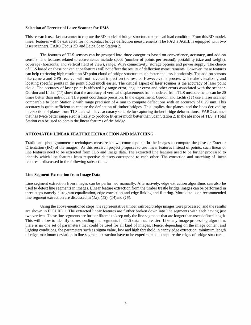
Line segment extraction from images can be performed manually. Alternatively, edge extraction algorithms can also be used to detect line segments in images. Linear feature extraction from the timber trestle bridge images can be performed in three steps namely histogram equalization, edge extraction and edge linking and filtering. More details on recommended line segment extraction are discussed in (12), (13), (14)and (15).

Using the above-mentioned steps, the representative timber railroad bridge images were processed, and the results are shown in FIGURE 1. The extracted linear features are further broken down into line segments with each having just two vertices. These line segments are further filtered to keep only the line segments that are longer than user-defined length. This will allow to identify corresponding line segments in TLS data much easier. Like any image processing algorithm, there is no one set of parameters that could be used for all kind of images. Hence, depending on the image content and lighting conditions, the parameters such as sigma value, low and high threshold in canny edge extraction, minimum length of edge, maximum deviation in line segment extraction have to be experimented to capture the edges of bridge structure.

5

FIGURE 1. Edges extracted from Canny algorithm overlaid on original grayscale image of bridge site 1: Three span timber trestle bridge - SV 849.90 (VL-Valrico)

Linear feature extraction from Terrestrial Laser Scanning (TLS) Data

Extracting linear features from 3D laser scanning data is a tedious process as compared to images due to additional dimensionality. There are various approaches that have been developed by the researchers for the linear features extraction from laser scanning data effectively and efficiently. The development of linear feature extraction methods from laser scanning data portrayed in different literatures can be mainly categorized into three groups. The first group is the spatial-domain approaches which can be achieved by region-grow based method (16) and model-fitting method (17). The second group, i.e. the parameter-domain approaches, are usually based on the geometric attributes of the linear features (18) where initially a Gaussian sphere of the point cloud has been constructed. This approach is not efficient from computational perspective to work with a massive amount of points. The third group i.e. hybrid approach is a combination of parameter domain approach and least squares line fitting procedure which is based on the Random Sample Consensus (RANSAC) algorithm (19) for detecting basic shapes in three-dimensional point-cloud. Although the algorithm is robust even with the presence of high degree of noise, this method is not efficient for many applications where finding shapes for every part of the surface is required. As for the experiments performed in this research, the extraction of linear features was achieved by plane-plane intersection, where planes were automatically extracted using seed points and region grow algorithm.

Linear Feature Matching

Once the linear features have been extracted from images and TLS data, the next step is to establish a feature matching algorithm to identify corresponding line segments. It is best achieved if the user identifies the corresponding line segments manually from the line segments extracted from images and TLS data. However, there are image processing algorithms that can perform matching with good approximation of Exterior Orientation (EO) of cameras. In the field of computer vision and image processing, image matching is a sub domain of computer vision which is fundamental for many applications such as motion analysis, scene reconstruction, image restoration, recovering the 3D scene structure from 2D images and robotic navigation (23), (24) and (25). Image matching algorithms are mainly focused on finding the similar features on a set of different images of the same object and eventually matching them. In feature-based matching, two corresponding features of the same object are paired together according to some measures of similarity. The points and lines are the two commonly used features in stereo matching process (26).

Mostly researchers use local interest points as a basis for image matching i.e. point-based image matching (27), (28), (29) and (30) which require feature points extraction from images and then image matching task is performed with extracted points. Alternatively, line segments can easily be identified in man-made structures like bridges. In some cases, line features are more advantageous than feature points in recovering three-dimensional object structure (31). Feature points-based image matching has limitation for poorly textured scene because points are hard to be detected and matched.

6

Whereas, line-based matching could be a better choice for recovering three-dimensional structure and can be easily outlined by several edge line segments (32). Despite the fact that the line-based image matching has advantages over the point-based image matching, line-based image matching has been less investigated as it is a difficult task due to the loss of connectivity and completeness of the extracted line segments.

Line matching method can be classified into two categories – 1) individual line segment matching and 2) line segment matches in a group. Some researchers used photometric information such as intensity (33), (34), gradient (35), (36), (37) and color (32) associated with the line segments to match individual line in different images. But the photometric information can produce false matches if there is not much variation in intensity, gradient or color in some of the line segments. Some researchers used geometric information rather than photometric information in the local regions around line segments for line matching (38). But it also uses the point features for line segments matching which is again a disadvantage for poorly textured images. Kim and Lee (39) worked on the group matching of line segments rather than individual line segment. This method is more complex which uses some strategies to intersect line segments to form junction points and then utilizes features associated with the generated junction points for line segment matching. But extracting the features associated in the junction points effectively to help matching is not an easy task. Fränti et al. (40) have proposed using the Hough transform for content-based matching in line-drawing images.

IMPLEMENTATION OF LINEAR FEATURE-BASED IMAGE REGISTRATION

Photogrammetry has been used for structural monitoring applications for more than three decades. Some of the typical challenges in using conventional photogrammetric techniques for structural applications are: 1) requirement of control points or targets, 2) access to the scene to place the targets and 3) typically a 2D information. Though the extraction of 3D information is possible with stereo images, it is often difficult to match points when the texture of the structure is homogeneous. Despite the limitations, the unique advantage of using images is the ability to capture the scene of interest in a fraction of a second. This advantage allows monitoring sudden structural changes in beams. In addition, specific points of interest can be better picked or measured as compared to laser scanning data.

Linear Feature-based Computation of EO

As an alternative to conventional point based photogrammetric procedures, this project demonstrates a method of extracting linear segments from TLS data to register the images collected by the camera that intends to measure the deflection in the structure of interest. As man-made structures have abundant linear features, it is a feasible method. There have been other researches where linear features were used to derive EO of the camera. Habib et al., (41) determined the orientation of a camera using free-form linear features as control. This approach does not require full correspondence of feature points, but it still requires that at least a few point correspondences exist for successful registration. Schenk (42) also demonstrated a line-based aerial triangulation technique by parameterizing straight lines in 3D space and assuming that the object space point and the back-projected image point are collinear. Habib et al., (43) used a similar straight-line-based registration, but with a different representation of a line. Akav et al., (44) demonstrated an aerial triangulation method using planar curves. This method does not require point correspondences but assumes that the feature is a mathematically perfect curve. Zhang et al., (45) computed relative orientation of images using multiple features such as points, straight lines and circles. The author uses a mathematical model of co-planarity condition for the vertical and horizontal straight lines, and center of the circle for circular curves. The above point-based and linear feature-based methods work under the assumption that the same point or parametric line can be identified in multi-sensor datasets such as images and TLS data. Hence, this project demonstrates a method that does not parametrize the line segments and instead takes all data points that represent them in the mathematical model to determine the EO of the cameras. Upon extracting linear segments from images and TLS data using manual or automatic procedures, the mathematical model for computing EO of images needs to be modified to accommodate such features. Then by minimizing the area formed between corresponding linear features, EO of the images are determined. This process is called as Area Minimization (AM) (46). The computed EO is further used to determine lateral and vertical deflections of any structural element due to load.

Camera Calibration

Camera calibration is the process of determining camera parameters such as calibrated focal length, principal point offset, radial and tangential distortion and image resolution. These values are also referred as Interior Orientation (IO) parameters. Despite some of these values are provided by the camera manufacturers, those are typically nominal values and need to be precisely determined for accurate mapping and monitoring applications. In addition, the commercial grade camera such as

7

the one recommended in this project are non-metric and hence requires frequent calibrations. The suitable calibration methods for this research include test field calibration (47), (48) and self-calibration (49).

DEVELOPMENT OF DEFLECTION MEASUREMENT METHODOLOGY USING DMS

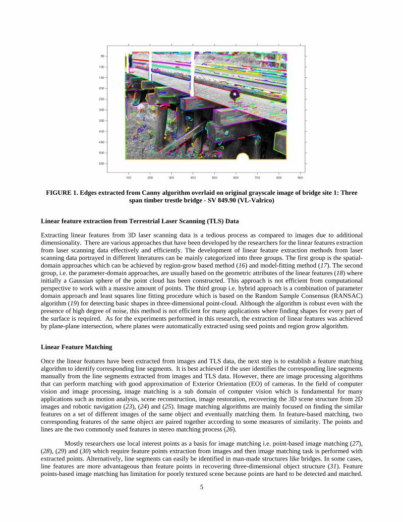
After the orientations of the cameras were determined from linear feature-based registration techniques, it is assumed that camera locations are fixed. This ensures that the camera orientation is a constant during dynamic loading procedure and need not be recomputed again. FIGURE 2 summarizes the camera Exterior Orientation (EO) methodology that is adopted in this research project. It should be noted that the 3D laser scanning (shown in green in FIGURE 2) of the bridge structure can be done independently prior to carrying-out the non-contact deflection measurement. Upon computing EO of images from one or more cameras, the deflection needs to be measured on specific points of interest. Typically, the maintenance engineer would be interested in measuring deflections at typical critical sections along the span. These sample points (mid-span, quarter-span, etc.) for deflection measurements can be automatically detected using the 3D laser scan or manually marked by the engineer on the bridge structure. The bridge maintenance engineer may also be interested in measuring deflection on arbitrary points where there are potential anomalies in the structure such as damage, crack, etc. These points are best identified manually. After identifying the points where deflection is needed, those sample points are tracked in multiple time series images that were taken during the dynamic load application. This task is referred as feature tracking. Tracking the same point along multiple time-series images is best achieved automatically as compared to manual identification. The following section discusses the feature tracking algorithms relevant for timber railroad bridges.

Feature Tracking

Feature tracking is the process of identifying the trajectory of identical points in multiple time-series images. Feature tracking is widely used in automatic detection of human actions or body movements with the advent of computer vision techniques. This process avoids same points to be manually identified in multiple image frames. The feature tracking has two major steps namely image matching and trajectory determination. There are several image matching algorithms available in the literature. They could be categorized as marker-based matching and natural point-based matching. The method of using artificial markers is suitable for the objects where fewer to no identifiable variations in the pixel values are found (e.g. steel structure). If there are enough information in the pixel (color) value that can uniquely identify the point of interest, then pixel or area based matching methods can be used. Area based matching uses values of all pixels in the given user-defined window, referred as template window. The most common area-based method is the cross-correlation based matching. It computes the cross-correlation coefficient between template and matches windows to identify the image segment with maximum correlation. The center pixel of the maximum correlation match window is considered as a match point or pixel. The search area for potential match windows are defined differently based on the object scene of interest. As for feature tracking in bridge deflection studies, the potential areas of match window can be defined by the expected maximum deflection. The factors and parameters that affect the correlation-based matching are discussed in Schenk (9) (pp 246-255).

FIGURE 2. Methodology flow-chart for exterior orientation computation

Dead load condition of the structure

Extract corresponding 3D lines from laser point

cloud Extract 2D lines from the picture

Determine EOP of the image by Feature-based registration

Take a picture of the structure

Dead load condition of the structure

3D laser scanning of the structure

8

Instead of using cross-correlation, least squares matching determines the match pixel location analytically by minimizing the differences in pixel (color or gray) values between template and match windows (47), (48). This method iteratively moves the location of match window to where minimum pixel value differences are achieved. It uses affine transformation where the parameters for scale, rotation, translational and shearing are determined by least squares adjustment. D'Apuzzo et al (49) used this least squares matching and tracking algorithm LSMTA (Least Squares Matching Tracking Algorithm) for human body modeling. The project team will use the LSMTA to track the points of interest in timber railroad bridges where deflection needs to be determined. The details of Least Squares Matching are discussed in Schenk (9), pp 251-257. This method is analogous to affine motion in computer vision (50).

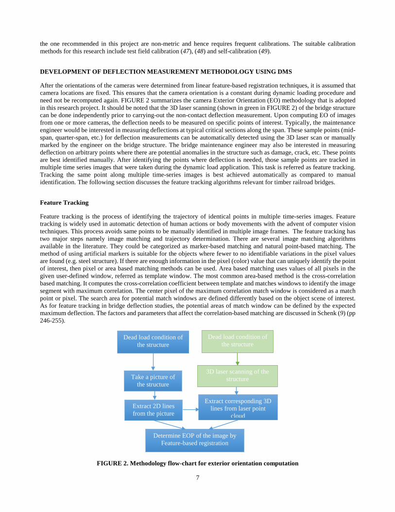
2D Deflection Methodology

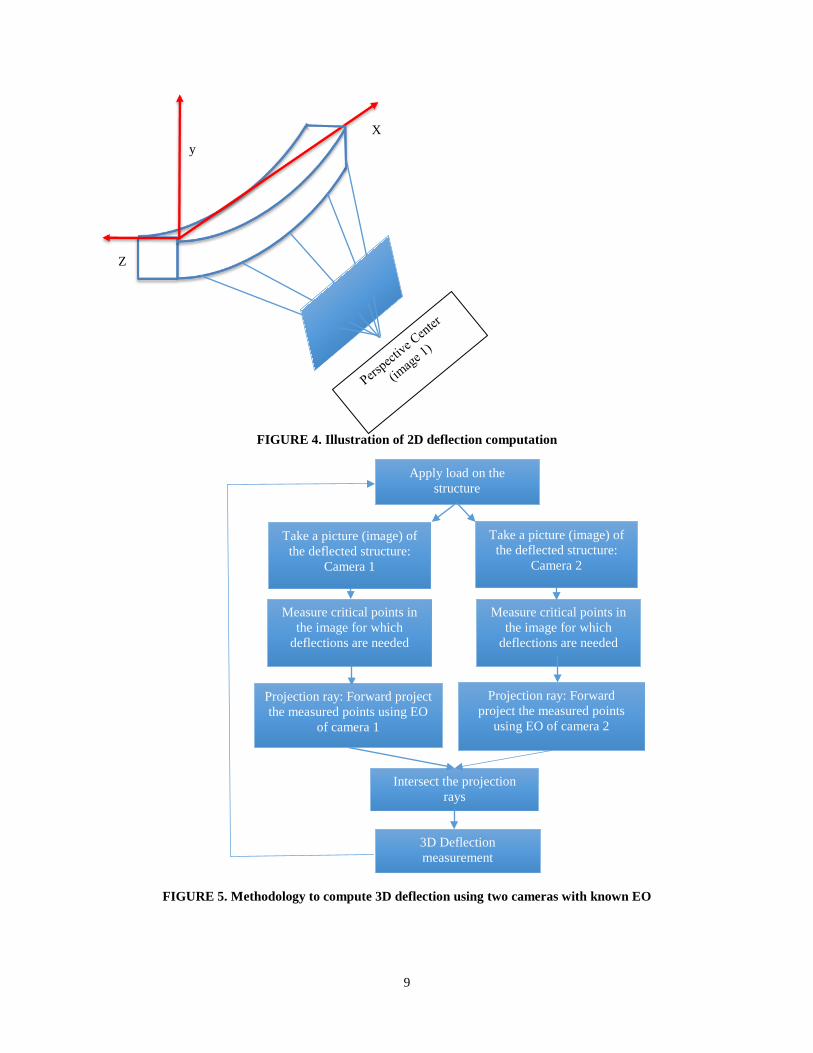
When a single camera is used for deflection measurement, only 2D deflection can be determined. It is achieved by generating a projection ray that originate from the perspective center of the camera and passing through the image point for which deflection is measured. If there exists a 3D model of the bridge in deflected position, the projection ray can be intersected with the deflected bridge surface to get 3D deflection. In the absence of 3D model of the bridge in deflected position, it is assumed that the deflection is happening only in the vertical direction and the frontal plane of the bridge can be extended infinitely. Then by using plane-ray intersection, the coordinates of deflected point on the frontal 2D plane can be determined. The methodology to compute 2D deflection is illustrated in FIGURE 3 and FIGURE 4.

3D Deflection Methodology

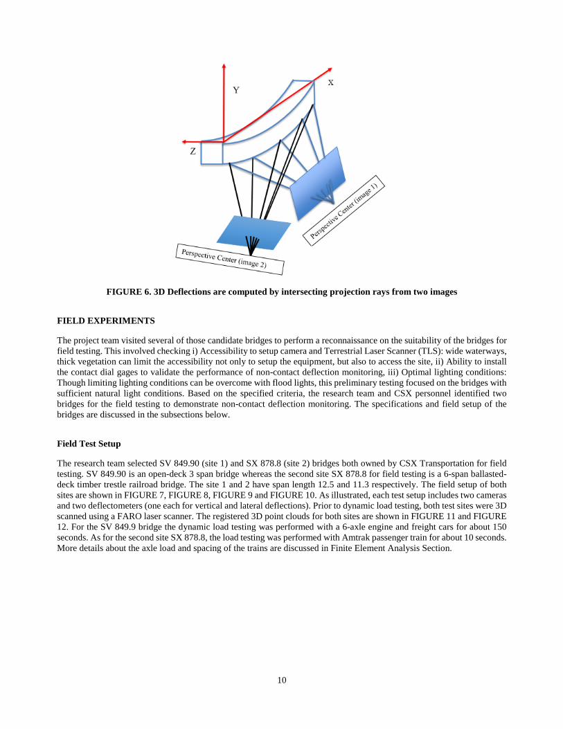
When two or more cameras are used for deflection measurement, 3D deflection (vertical and lateral deflections) can be determined. It is achieved by generating a projection ray for each of the cameras that originate from their respective perspective centers and pass through the image point for which deflection is measured. The projection rays are intersected in object space (3D space) to determine the 3D coordinate of deflected points. There are also alternative least squares-based solutions available to determine the 3D coordinates of deflected points (54). The methodology of 3D deflection computation is illustrated in FIGURE 5 and FIGURE 6.

FIGURE 3. Methodology to compute 2D deflection using a single camera with known EO

Apply load on the structure

Measure critical points in the image for which deflections are needed

EO computed in dead load condition

Extract frontal plane of the beam from TLS data collected in dead load

condition

Projection ray: Forward project the measured points using EO

Intersect the projection ray with frontal plane of the beam

Deflection measurement

Take a picture (image) of the deflected structure

9

FIGURE 4. Illustration of 2D deflection computation

FIGURE 5. Methodology to compute 3D deflection using two cameras with known EO

Apply load on the structure

Projection ray: Forward project the measured points

using EO of camera 2

Intersect the projection rays

3D Deflection measurement

Measure critical points in the image for which

deflections are needed

Projection ray: Forward project the measured points using EO

of camera 1

Take a picture (image) of the deflected structure:

Camera 1

Measure critical points in the image for which

deflections are needed

Take a picture (image) of the deflected structure:

Camera 2

X

Z

y

10

FIGURE 6. 3D Deflections are computed by intersecting projection rays from two images

FIELD EXPERIMENTS

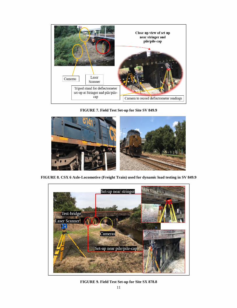
The project team visited several of those candidate bridges to perform a reconnaissance on the suitability of the bridges for field testing. This involved checking i) Accessibility to setup camera and Terrestrial Laser Scanner (TLS): wide waterways, thick vegetation can limit the accessibility not only to setup the equipment, but also to access the site, ii) Ability to install the contact dial gages to validate the performance of non-contact deflection monitoring, iii) Optimal lighting conditions: Though limiting lighting conditions can be overcome with flood lights, this preliminary testing focused on the bridges with sufficient natural light conditions. Based on the specified criteria, the research team and CSX personnel identified two bridges for the field testing to demonstrate non-contact deflection monitoring. The specifications and field setup of the bridges are discussed in the subsections below.

Field Test Setup

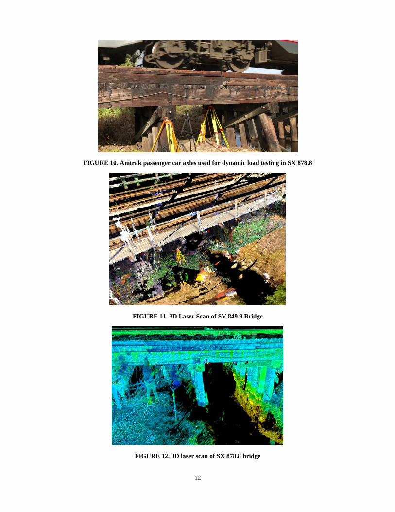
The research team selected SV 849.90 (site 1) and SX 878.8 (site 2) bridges both owned by CSX Transportation for field testing. SV 849.90 is an open-deck 3 span bridge whereas the second site SX 878.8 for field testing is a 6-span ballasted-deck timber trestle railroad bridge. The site 1 and 2 have span length 12.5 and 11.3 respectively. The field setup of both sites are shown in FIGURE 7, FIGURE 8, FIGURE 9 and FIGURE 10. As illustrated, each test setup includes two cameras and two deflectometers (one each for vertical and lateral deflections). Prior to dynamic load testing, both test sites were 3D scanned using a FARO laser scanner. The registered 3D point clouds for both sites are shown in FIGURE 11 and FIGURE 12. For the SV 849.9 bridge the dynamic load testing was performed with a 6-axle engine and freight cars for about 150 seconds. As for the second site SX 878.8, the load testing was performed with Amtrak passenger train for about 10 seconds. More details about the axle load and spacing of the trains are discussed in Finite Element Analysis Section.

11

FIGURE 7. Field Test Set-up for Site SV 849.9

FIGURE 8. CSX 6 Axle-Locomotive (Freight Train) used for dynamic load testing in SV 849.9

FIGURE 9. Field Test Set-up for Site SX 878.8

12

FIGURE 10. Amtrak passenger car axles used for dynamic load testing in SX 878.8

FIGURE 11. 3D Laser Scan of SV 849.9 Bridge

FIGURE 12. 3D laser scan of SX 878.8 bridge

13

Non-Contact Deflection Results

As shown in FIGURE 7 and FIGURE 9, the cameras and the deflectometer readings were turned on a few minutes before the application of the moving train loads. The cameras captured the data in video mode with 30 frames per second (fps). After the train had completely passed off the bridge, the videos were ended. These videos were converted to images (or individual frames) for further processing of deflection measurements.

Processing of SV 849.9 Bridge Data:

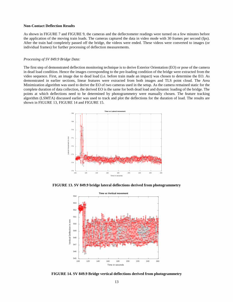
The first step of demonstrated deflection monitoring technique is to derive Exterior Orientation (EO) or pose of the camera in dead load condition. Hence the images corresponding to the pre-loading condition of the bridge were extracted from the video sequence. First, an image due to dead load (i.e. before train made an impact) was chosen to determine the EO. As demonstrated in earlier sections, linear features were extracted from both images and TLS point cloud. The Area Minimization algorithm was used to derive the EO of two cameras used in the setup. As the camera remained static for the complete duration of data collection, the derived EO is the same for both dead load and dynamic loading of the bridge. The points at which deflections need to be determined by photogrammetry were manually chosen. The feature tracking algorithm (LSMTA) discussed earlier was used to track and plot the deflections for the duration of load. The results are shown in FIGURE 13, FIGURE 14 and FIGURE 15.

FIGURE 13. SV 849.9 bridge lateral deflections derived from photogrammetry

FIGURE 14. SV 849.9 Bridge vertical deflections derived from photogrammetry

100 120 140 160 180 200 220 240 260

Time in seconds

-775

-774

-773

-772

-771

-770

-769

-768

Late

ral m

ovem

ent i

n m

m

Time vs Lateral movement

100 120 140 160 180 200 220 240 260

Time in seconds

545

546

547

548

549

550

551

552

553

554

Ver

tical

Def

lect

ion

in m

m

Time vs Vertical movement

14

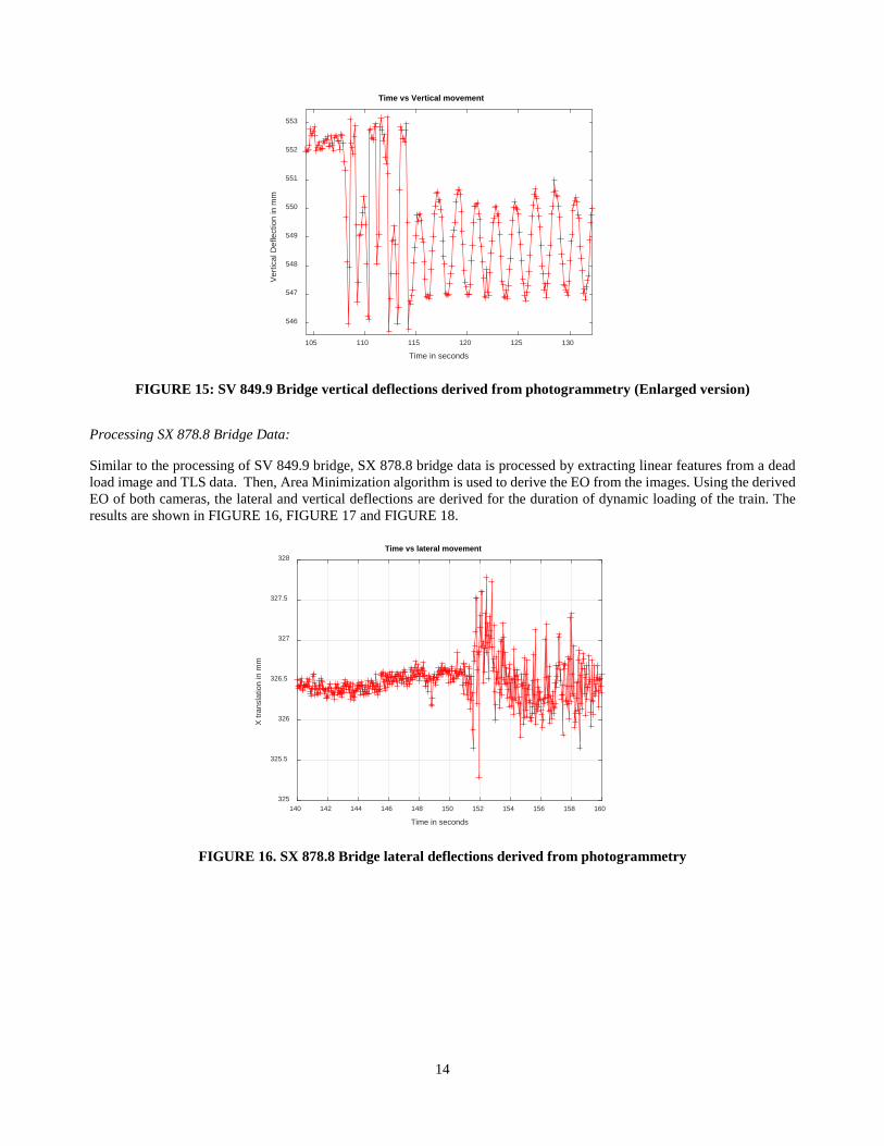
FIGURE 15: SV 849.9 Bridge vertical deflections derived from photogrammetry (Enlarged version)

Processing SX 878.8 Bridge Data:

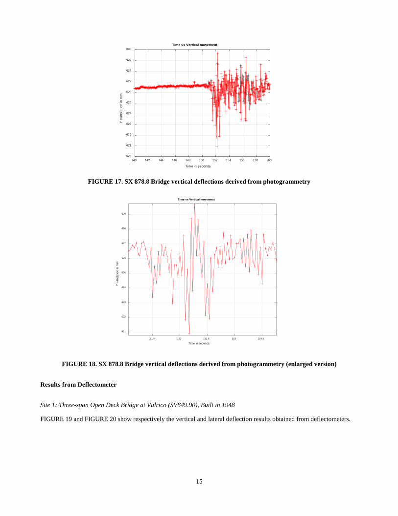
Similar to the processing of SV 849.9 bridge, SX 878.8 bridge data is processed by extracting linear features from a dead load image and TLS data. Then, Area Minimization algorithm is used to derive the EO from the images. Using the derived EO of both cameras, the lateral and vertical deflections are derived for the duration of dynamic loading of the train. The results are shown in FIGURE 16, FIGURE 17 and FIGURE 18.

FIGURE 16. SX 878.8 Bridge lateral deflections derived from photogrammetry

105 110 115 120 125 130

Time in seconds

546

547

548

549

550

551

552

553

Ver

tical

Def

lect

ion

in m

m

Time vs Vertical movement

140 142 144 146 148 150 152 154 156 158 160

Time in seconds

325

325.5

326

326.5

327

327.5

328

X tr

ansl

atio

n in

mm

Time vs lateral movement

15

FIGURE 17. SX 878.8 Bridge vertical deflections derived from photogrammetry

FIGURE 18. SX 878.8 Bridge vertical deflections derived from photogrammetry (enlarged version)

Results from Deflectometer

Site 1: Three-span Open Deck Bridge at Valrico (SV849.90), Built in 1948

FIGURE 19 and FIGURE 20 show respectively the vertical and lateral deflection results obtained from deflectometers.

140 142 144 146 148 150 152 154 156 158 160

Time in seconds

620

621

622

623

624

625

626

627

628

629

630

Y tr

ansl

atio

n in

mm

Time vs Vertical movement

151.5 152 152.5 153 153.5

Time in seconds

621

622

623

624

625

626

627

628

629

Y tr

ansl

atio

n in

mm

Time vs Vertical movement

16

FIGURE 19.Vertical displacement of stringer from deflectometer

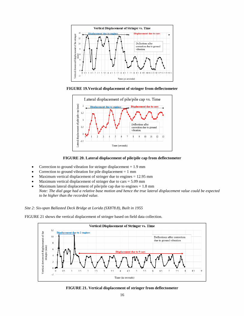
FIGURE 20. Lateral displacement of pile/pile cap from deflectometer

• Correction to ground vibration for stringer displacement = 1.9 mm • Correction to ground vibration for pile displacement = 1 mm • Maximum vertical displacement of stringer due to engines = 12.95 mm • Maximum vertical displacement of stringer due to cars = 5.09 mm • Maximum lateral displacement of pile/pile cap due to engines = 1.8 mm

Note: The dial gage had a relative base motion and hence the true lateral displacement value could be expected to be higher than the recorded value.

Site 2: Six-span Ballasted Deck Bridge at Lorida (SX878.8), Built in 1955

FIGURE 21 shows the vertical displacement of stringer based on field data collection.

FIGURE 21. Vertical displacement of stringer from deflectometer

17

• Correction to ground vibration for stringer deflection = 0.39 mm • Correction to ground vibration for pile deflection = 0.05 mm • Maximum vertical displacement of stringer due to engines = 10.25 mm • Maximum vertical displacement of stringer due to cars = 4.28 mm • Maximum lateral displacement of pile/pile cap due to engines = 0.5 mm

Corrections to Train-induced Ground Vibration

A ground-borne vibration model for rail systems at-grade has been developed by Cardona et. al. (55) and validated with experimental measurements in an existing commuter railway line. This model was based on a semi-analytical characterization of the wave propagation. This model was able to predict the vibration field that will be caused by railway infrastructure. The present study incorporates a correction to the train-induced ground vibration to the recorded dial gage deflection measurements.

FINITE ELEMENT ANALYSIS

(Analysis based on idealization of stringers and piles without any cracks)

Moving live load analysis is performed for open deck and ballasted deck timber trestle railroad bridge model using CSIBridge software. The dimensions of the bridge model are based on the field data collected for Valrico bridge near Tampa SV 849.90 (VL-Valrico), built in 1948 and Lorida bridge (SX878.8), built in 1955. The aim of the analysis is to obtain vertical deflection of the stringer at the mid-span due to moving loads. Static analysis is performed to obtain lateral deflection of pile due to nosing of the locomotive. These results are compared with the deflection obtained from the field tests and the proposed non-contact deflection monitoring system. TABLE 1 shows the material and geometric properties of timber trestle railroad bridge structural elements used in the analysis.

TABLE 1. Material and Geometric Properties of Timber Trestle Bridge

Decay of timber is not considered Material properties for bridges in site 1 and site 2 Timber type Red Oak Weight per unit volume 3.96E-05 (kip/in3) Modulus of elasticity 1200 (kip/in2) Poisson’s ratio 0.29 Coefficient of thermal expansion 2.7E-06 (in./in. deg F) Geometric sizes for bridges in site 1 and site 2 Nominal sizes Dressed sizes Pile diameter 14 inches 13.5 inches Cap beam cross section (width by depth) 14” x 14” 13.5” x 13.5” Diagonal brace cross section (width by depth) 8” x 4” 7.5” x 3.5” Ties (width by depth by length) 8” x 8” x 10’ 7.5” x 7.5” x 10’ Stringer cross section (width by depth) for site 1 32” x 15” 32” x 14.5” Stringer cross section (width by depth) for site 2 8” x 20” 8” x 19.5”

Site 1: Three-span Open Deck Bridge at Valrico (SV849.90), Built in 1948

Modeling of timber trestle railroad bridge is done using CSIBrisge Finite Element Analysis software based on field data. FIGURE 22 shows 3D view of the analytical model. The height of the trestle bent is 7 feet. Based on Ali F. Jwary (56), the piles are extended to 25 feet below the soil. The data and calculation method for equivalent soil spring is based on David R. Bonhoff (57). Axle loads and spacings used in the FEM analysis is shown in FIGURE 23. As for the lateral loads, nosing of locomotive shall be considered as a moving concentrated load of 20 kips applied at the top of the rail in either direction

18

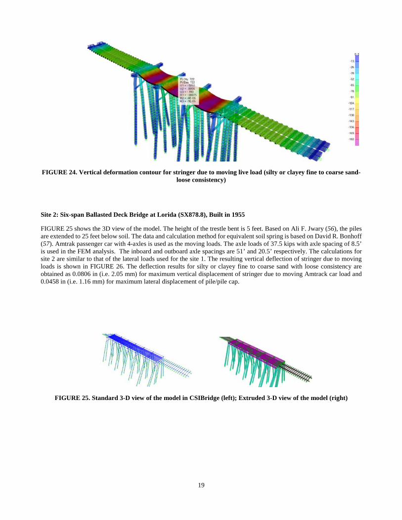
at any point in the span (3). Considering the typical depth of rail cross section as 2.75 inches, the moment on top of the stringer is obtained as: 𝑀𝑀𝑦𝑦 = 20 × 2.75 = 55 𝑘𝑘𝑘𝑘𝑘𝑘 − 𝑘𝑘𝑖𝑖. Hence the lateral force (Fx) of 20 kip and Moment (𝑀𝑀𝑦𝑦) of 55 k-in is applied on top of the stringer located above the bent. Vertical deflection of stringer due to moving loads is shown in FIGURE 31. The deflection results for silty or clayey fine to coarse sand with loose consistency are obtained as 0.193 in (i.e. 4.90 mm) for maximum vertical displacement of stringer due to moving engine load and 0.0525 in (i.e. 1.33 mm) for maximum lateral displacement of pile/pile cap.

FIGURE 22. 3D view of the analytical model

FIGURE 23. Axle load and spacing

19

FIGURE 24. Vertical deformation contour for stringer due to moving live load (silty or clayey fine to coarse sand- loose consistency)

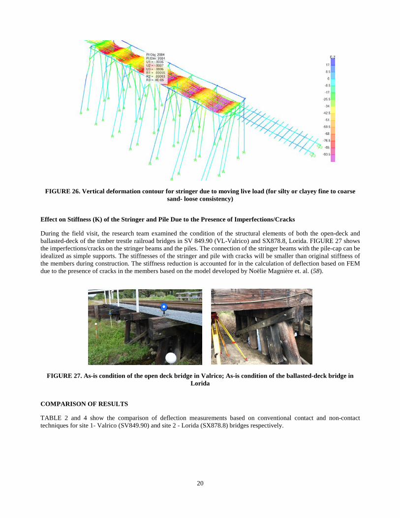
Site 2: Six-span Ballasted Deck Bridge at Lorida (SX878.8), Built in 1955

FIGURE 25 shows the 3D view of the model. The height of the trestle bent is 5 feet. Based on Ali F. Jwary (56), the piles are extended to 25 feet below soil. The data and calculation method for equivalent soil spring is based on David R. Bonhoff (57). Amtrak passenger car with 4-axles is used as the moving loads. The axle loads of 37.5 kips with axle spacing of 8.5’ is used in the FEM analysis. The inboard and outboard axle spacings are 51’ and 20.5’ respectively. The calculations for site 2 are similar to that of the lateral loads used for the site 1. The resulting vertical deflection of stringer due to moving loads is shown in FIGURE 26. The deflection results for silty or clayey fine to coarse sand with loose consistency are obtained as 0.0806 in (i.e. 2.05 mm) for maximum vertical displacement of stringer due to moving Amtrack car load and 0.0458 in (i.e. 1.16 mm) for maximum lateral displacement of pile/pile cap.

FIGURE 25. Standard 3-D view of the model in CSIBridge (left); Extruded 3-D view of the model (right)

20

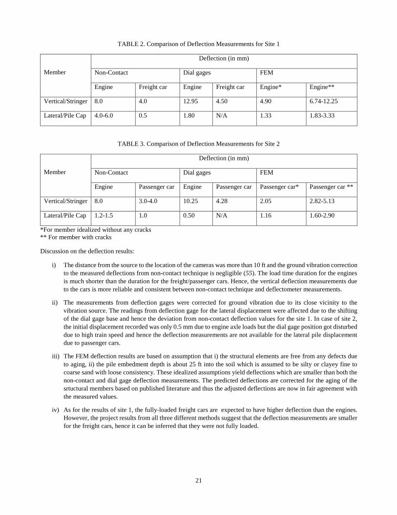
FIGURE 26. Vertical deformation contour for stringer due to moving live load (for silty or clayey fine to coarse sand- loose consistency)

Effect on Stiffness (K) of the Stringer and Pile Due to the Presence of Imperfections/Cracks

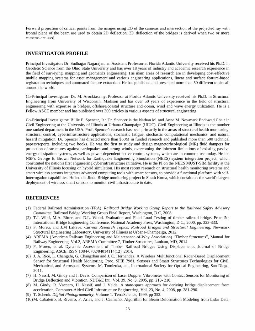
During the field visit, the research team examined the condition of the structural elements of both the open-deck and ballasted-deck of the timber trestle railroad bridges in SV 849.90 (VL-Valrico) and SX878.8, Lorida. FIGURE 27 shows the imperfections/cracks on the stringer beams and the piles. The connection of the stringer beams with the pile-cap can be idealized as simple supports. The stiffnesses of the stringer and pile with cracks will be smaller than original stiffness of the members during construction. The stiffness reduction is accounted for in the calculation of deflection based on FEM due to the presence of cracks in the members based on the model developed by Noëlie Magnière et. al. (58).

FIGURE 27. As-is condition of the open deck bridge in Valrico; As-is condition of the ballasted-deck bridge in Lorida

COMPARISON OF RESULTS

TABLE 2 and 4 show the comparison of deflection measurements based on conventional contact and non-contact techniques for site 1- Valrico (SV849.90) and site 2 - Lorida (SX878.8) bridges respectively.

21

TABLE 2. Comparison of Deflection Measurements for Site 1

Member

Deflection (in mm)

Non-Contact Dial gages FEM

Engine Freight car Engine Freight car Engine* Engine**

Vertical/Stringer 8.0 4.0 12.95 4.50 4.90 6.74-12.25

Lateral/Pile Cap 4.0-6.0 0.5 1.80 N/A 1.33 1.83-3.33

TABLE 3. Comparison of Deflection Measurements for Site 2

Member

Deflection (in mm)

Non-Contact Dial gages FEM

Engine Passenger car Engine Passenger car Passenger car* Passenger car **

Vertical/Stringer 8.0 3.0-4.0 10.25 4.28 2.05 2.82-5.13

Lateral/Pile Cap 1.2-1.5 1.0 0.50 N/A 1.16 1.60-2.90

*For member idealized without any cracks ** For member with cracks

Discussion on the deflection results:

i) The distance from the source to the location of the cameras was more than 10 ft and the ground vibration correction to the measured deflections from non-contact technique is negligible (55). The load time duration for the engines is much shorter than the duration for the freight/passenger cars. Hence, the vertical deflection measurements due to the cars is more reliable and consistent between non-contact technique and deflectometer measurements.

ii) The measurements from deflection gages were corrected for ground vibration due to its close vicinity to the vibration source. The readings from deflection gage for the lateral displacement were affected due to the shifting of the dial gage base and hence the deviation from non-contact deflection values for the site 1. In case of site 2, the initial displacement recorded was only 0.5 mm due to engine axle loads but the dial gage position got disturbed due to high train speed and hence the deflection measurements are not available for the lateral pile displacement due to passenger cars.

iii) The FEM deflection results are based on assumption that i) the structural elements are free from any defects due to aging, ii) the pile embedment depth is about 25 ft into the soil which is assumed to be silty or clayey fine to coarse sand with loose consistency. These idealized assumptions yield deflections which are smaller than both the non-contact and dial gage deflection measurements. The predicted deflections are corrected for the aging of the srtuctural members based on published literature and thus the adjusted deflections are now in fair agreement with the measured values.

iv) As for the results of site 1, the fully-loaded freight cars are expected to have higher deflection than the engines. However, the project results from all three different methods suggest that the deflection measurements are smaller for the freight cars, hence it can be inferred that they were not fully loaded.

22

PLANS FOR IMPLEMENTATION

The project investigators developed the non-contact deflection techniques and successfully demonstrated the feasibility through field testing. The next step is to reach out to the railroad timber bridge owners in the nation to demonstrate the methodology and share the developed techniques, methodologies, and results with them for a potential implementation in their maintenance practice.

In addition, the results and methodologies will be presented in national conferences, published in national newsletters and journals for a broader outreach. As a proof-of-concept, the research team implemented the project methodology in Matlab as a sequence of multiple individual scripts. These scripts are available to the users upon request. However, depending on the familiarity of users with Matlab, the implementation may or may not take longer. Hence, the research team plans on developing a user-friendly commercial grade software product in the future to make the implementation process easier for any users.

The project team expect that the project can be implemented by the bridge maintenance team. The typical sequence of field implementation will be as follows.

Step 1: The bridge maintenance technician will use a laser scanner or total station to capture linear features on the bridge structure with at least three of them are mutually perpendicular. The collection of these linear features is a one-time process that is needed once per bridge which can be performed in a day of convenience.

Step 2: On the day of bridge deflection measurement, the technician will setup the camera(s) in the field on a tripod to ensure the area where deflection needs to be measured is in the field of view. It is ideal that the camera is kept in video capture mode and the video recording be turned on a minute or more before the train-bridge impact.

Step 3: After the train fully passes the bridge, the video recording can be turned off. This way of recording will ensure that the bridge is captured in both dead load and dynamic loading conditions.

Step 4: After the videos (or image sequences) are captured by the camera(s), the data will be downloaded and loaded in a computer with Matlab. The scripts created by the project team can be used to extract linear features from one dead load image. The corresponding linear features will be extracted from laser scanning or total station data. The linear features extraction can be done both manually or automatically.

Step 5: Then the pose or Exterior Orientation of the camera will be determined using the Area Minimization algorithm script developed by the project team.

Step 6: The user, typically the maintenance technician/engineer/structural engineer will pick points on the image in Matlab where deflection needs to be measured during the dynamic loading by the train. The feature tracking algorithm and the corresponding script developed by the project team can be used to track the points of interest in all image sequences automatically to generate the plot of how bridge deflected in 2D/3D during the loading. For example, the duration of two minutes of train on the bridge at 30 fps (frames per second) will produce 2x60x30=3600 images. It is practically impossible for the user to identify the same point in all these images manually. Hence the tracking algorithm will assist the user to generate the plots similar to FIGURE 13.

CONCLUSIONS

This study establishes a method of monitoring the deformations of timber trestle railroad bridges using non-contact methodology based on both Photogrammetry and Terrestrial Laser Scanner. The measured deformations from the non-contact methodology are compared with those recorded by conventional dial gages and analytical results from Finite Element modeling. The comparison shows a fair agreement with the measured values by dial gages and computed deflections using FEM. The FEM model takes into account the effect of soil-pile interaction based on the p-y curve originally developed by Reese et. al. The imperfections/cracks in the stringer and pile are accounted for in the deflection values from FEM. The measured deflections of key structural elements of the timber trestle bridges are adjusted to take into account the effect of ground vibrations from the moving engine and freight/passenger car loads.

This non-contact measurement technique involves a method of extracting linear features from both images and TLS data. Exterior Orientation (EO) of the images are derived by using a linear feature-based registration algorithm.

23

Forward projection of critical points from the images using EO of the cameras and intersection of the projected ray with frontal plane of the beam are used to obtain 2D deflection. 3D deflection of the bridges is derived when two or more cameras are used.

INVESTIGATOR PROFILE

Principal Investigator: Dr. Sudhagar Nagarajan, an Assistant Professor at Florida Atlantic University received his Ph.D. in Geodetic Science from the Ohio State University and has over 18 years of industry and academic research experience in the field of surveying, mapping and geomatics engineering. His main areas of research are in developing cost-effective mobile mapping systems for asset management and various engineering applications, linear and surface feature-based registration techniques and automated feature extraction. He has published and presented more than 50 different topics all around the world.

Co-Principal Investigator: Dr. M. Arockiasamy, Professor at Florida Atlantic University received his Ph.D. in Structural Engineering from University of Wisconsin, Madison and has over 50 years of experience in the field of structural engineering with expertise in bridges, offshore/coastal structure and ocean, wind and wave energy utilization. He is a Fellow ASCE member and has published over 300 articles in various aspects of structural engineering.

Co-Principal Investigator: Billie F. Spencer, Jr.: Dr. Spencer is the Nathan M. and Anne M. Newmark Endowed Chair in Civil Engineering at the University of Illinois at Urbana-Champaign (UIUC). Civil Engineering at Illinois is the number one ranked department in the USA. Prof. Spencer's research has been primarily in the areas of structural health monitoring, structural control, cyberinfrastructure applications, stochastic fatigue, stochastic computational mechanics, and natural hazard mitigation. Dr. Spencer has directed more than $50M in funded research and published more than 500 technical papers/reports, including two books. He was the first to study and design magnetorheological (MR) fluid dampers for protection of structures against earthquakes and strong winds, overcoming the inherent limitations of existing passive energy dissipation systems, as well as power-dependent active control systems, which are in common use today. He led NSF's George E. Brown Network for Earthquake Engineering Simulation (NEES) system integration project, which constituted the nation's first engineering cyberinfrastructure initiative. He is the PI on the NEES MUST-SIM facility at the University of Illinois focusing on hybrid simulation. His most recent research on structural health monitoring systems and smart wireless sensors integrates advanced computing tools with smart sensors, to provide a functional platform with self-interrogation capabilities. He led the Jindo Bridge monitoring project in South Korea, which constitutes the world's largest deployment of wireless smart sensors to monitor civil infrastructure to date.

REFERENCES

(1) Federal Railroad Administration (FRA). Railroad Bridge Working Group Report to the Railroad Safety Advisory Committee. Railroad Bridge Working Group Final Report, Washington, D.C, 2008.

(2) T.J. Wipf, M.A. Ritter, and D.L. Wood. Evaluation and Field Load Testing of timber railroad bridge. Proc. 5th International Bridge Engineering Conference, National Academy Press, Washington, D.C., 2000, pp. 323-333.

(3) F. Moreu, and J.M LaFave. Current Research Topics: Railroad Bridges and Structural Engineering. Newmark Structural Engineering Laboratory, University of Illinois at Urbana-Champaign, 2012.

(4) AREMA (American Railway Engineering and Maintenance-of-Way Association) “Timber Structures”, Manual for Railway Engineering, Vol.2, AREMA Committee 7, Timber Structures, Lanham, MD, 2014.

(5) F. Moreu, et al. Dynamic Assessment of Timber Railroad Bridges Using Displacements. Journal of Bridge Engineering, ASCE, ISSN 1084-0702/04014114(12), 2014.

(6) J. A. Rice, L. Changzhi, G. Changzhan and J. C. Hernandez. A Wireless Multifunctional Radar-Based Displacement Sensor for Structural Health Monitoring. Proc. SPIE 7981, Sensors and Smart Structures Technologies for Civil, Mechanical, and Aerospace Systems, M. Tomizuka, ed., International Society for Optical Engineering, San Diego, 2011.

(7) H. Nassif, M. Gindy and J. Davis. Comparison of Laser Doppler Vibrometer with Contact Sensors for Monitoring of Bridge Deflection and Vibration. NDT&E Int., Vol. 39, No. 3, 2005, pp. 213- 218.

(8) M. Gindy, R. Vaccaro, H. Nassif, and J. Velde. A state-space approach for deriving bridge displacement from acceleration. Computer-Aided Civil Infrastructure Engineering, Vol. 23, No. 4, 2008, pp. 281-290.

(9) T. Schenk. Digital Photogrammetry, Volume 1. TerraScience, 1999. pp 352. (10) M. Cabaleiro, B. Riveiro, P. Arias, and J. Caamaño. Algorithm for Beam Deformation Modeling from Lidar Data,

24

Measurement, 10.1016/j.measurement.2015.08.023, 2015, pp. 20-31. (11) S. Gordon and D. Lichti. Modeling Terrestrial Laser Scanner Data for Precise Structural Deformation Measurement.

J. Surv. Eng., 10.1061/(ASCE)0733-9453(2007)133:2(72), 2007, pp.72-80. (12) J. Canny. A Computational Approach to Edge Detection. IEEE Transactions on Pattern Analysis And Machine

Intelligence PAMI- Vol. 8, No. 6, 1986, pp. 679-98. (13) K. P. Karla. Canny Edge Detection, http://www.cse.iitd.ernet.in/~pkalra/col783/canny.pdf, 2009. (14) P. Kovesi. MATLAB and Octave Functions for Computer Vision and Image Processing. Available

from:<http://www.peterkovesi.com/matlabfns/>. Last Accessed on: Jan 30th 2018. (15) R. C. Gonzalez and R. E. Woods. Digital Image Processing. 2nd ed. Prentice Hall, 2002. (16) D. Belton and D. D. Lichti. Classification and Segmentation of Terrestrial Laser Scanner Point Clouds using Local

Variance Information. Int. Arch. Photogramm. Remote Sens. Spatial Inf. Sci, Vo. 36 N0. 5, 2006, pp. 44-49. (17) D. Marshall, G. Lukacs, and R. Martin. Robust segmentation of primitives from range data in the presence of geometric

degeneracy. IEEE Trans. Pattern Anal. Mach. Intell, Vol. 23, No. 3, 2001, pp. 304-314. (18) T. Rabbani. Automatic Reconstruction of Industrial Installations Using Point Clouds and Images. Civil Engineering

and Geosciences, TU Delft, 2006. (19) R. Schnabel, R. Wahl, and R. Klein. Efficient RANSAC for Point-Cloud Shape Detection. Comput. Graph. Forum,

Vol. 26 No. 2, 2007, pp. 214-226. (20) Z. Lari and A. Habi. An Adaptive Approach for the Segmentation and Extraction of Planar and Linear/Cylindrical

Features from Laser Scanning Data. ISPRS Journal of Photogrammetry and Remote Sensing, Vol. 93, 2014, pp. 192-212.

(21) N. Meierhold and A. Schmich, Referencing of images to laser scanner data using linear features extracted from digital images and range images. International Society for Photogrammetry and Remote Sensing, Vol. 38, No. 3/W8, 2010. pp. 164-170.

(22) H. Ma and C. Yao. A Novel Method for Linear Features Extraction from Raw Lidar Point Clouds. Multimedia Technology (ICMT), International Conference on IEEE. October 2010, pp. 1-3.

(23) D. Sankowski, J. Nowakowski, D. Sankowski, and J. Nowakowski. Computer vision in robotics and industrial applications. World Scientific Publishing Co., Inc. 2014

(24) W.E.L. Grimson, and J.L. Mundy. Computer vision applications. Communications of the ACM, Vol. 37, No. 3, 1994, pp.45-51.

(25) S. Kagami. High-Speed Vision Systems and Projectors for Real-Time Perception of the World. Computer Vision and Pattern Recognition Workshops (CVPRW), IEEE Computer Society Conference. June 2010, pp. 100-107.

(26) T. Fang-Chih and S. Te-Hsiu. Solving Line-Feature Stereo Matching with Genetic Algorithms in Hough space. Journal of the Chinese Institute of Industrial Engineers, 2004, pp. 516-526.

(27) Y. Ke and R. Sukthankar. PCA-SIFT: A More Distinctive Representation for Local Image Descriptors. Computer Vision and Pattern Recognition, CVPR, Proceedings of IEEE Computer Society Conference, Vol. 2, June 2004.

(28) D.G. Lowe. Distinctive Image Features from Scale-Invariant Key-points. International journal of computer vision, Vol. 60, No. 2, 2004, pp. 91-110.

(29) J.M. Morel and G. Yu. ASIFT: A New Framework for Fully Affine Invariant Image Comparison. SIAM Journal on Imaging Sciences, Vol. 2, No. 2, 2009, pp.438-469.

(30) Z. Wang, B. Fan and F. Wu. Local Intensity Order Pattern for Feature Description. Computer Vision (ICCV), IEEE International Conference, 2011, pp. 603-610.

(31) M. Chandraker, J. Lim and D. Kriegman, September. Moving in Stereo: Efficient Structure and Motion Using Lines. Computer Vision, 12th IEEE International Conference, 2009, pp. 1741-1748.

(32) H. Bay, A. Ess, A. Neubeck and L. Van Gool. 3D From Line Segments in Two Poorly-Textured, Uncalibrated Images. 3D Data Processing, Visualization, and Transmission, Third International Symposium, June 2006, pp. 496-503.

(33) C. Schmid and A. Zisserman. Automatic line matching across views. Computer Vision and Pattern Recognition, Proceedings of IEEE Computer Society Conference, June 1997, pp. 666-671.

(34) C. Baillard, C. Schmid, A. Zisserman, and A. Fitzgibbon. Automatic Line Matching and 3D Reconstruction of Buildings from Multiple Views. ISPRS Conference on Automatic Extraction of GIS Objects from Digital Imagery, Vol. 32, September 1999, pp. 69-80.

(35) B. Verhagen, R. Timofte, and L.Van Gool, March. Scale-Invariant Line Descriptors for Wide Baseline Matching. Applications of Computer Vision (WACV), IEEE Winter Conference, 2014, pp. 493-500.

(36) Z. Wang, F. Wu and Z. Hu. MSLD: A Robust Descriptor for Line Matching. Pattern Recognition, Vol. 42, No. 5, 2009, pp.941-953.

(37) L. Zhang and R. Koch. An Efficient and Robust Line Segment Matching Approach Based on LBD Descriptor and Pairwise Geometric Consistency. Journal of Visual Communication and Image Representation, Vol. 24, No.7, 2013, pp.794-805.

25

(38) M.I. Lourakis, S.T. Halkidis, and S.C. Orphanoudakis. Matching Disparate Views of Planar Surfaces using Projective Invariants. Image and Vision Computing, Vol. 18, No. 9, 2000, pp.673-683.

(39) H. Kim, and S. Lee. Simultaneous Line Matching and Epipolar Geometry Estimation Based on the Intersection Context of Coplanar Line Pairs. Pattern Recognition Letters, Vo. 33, No. 10, 2012, pp.1349-1363.

(40) P. Fränti, A. Mednonogov, V. Kyrki, and H. Kälviäinen, Content-Based Matching of Line-Drawing Images using the Hough Transform. International Journal on Document Analysis and Recognition, Vol. 3, No. 2, 2000, pp.117-124.

(41) A. Habib, S.W. Shin and M. Morgan. Automatic Pose Estimation Using Free-Form Control Linear Features. Proceedings of the International Archives of the Photogrammetry, Remote Sensing and Spatial Information Sciences, Graz, Austria, Vol. 34 No. 3A, September 9-13, 2002, pp. 150 – 155.

(42) T. Schenk. Point-based to Feature-based Aerial Triangulation. ISPRS Journal of Photogrammetry and Remote Sensing, Vol. 58, No. 5-6, 2004, pp. 315–329.

(43) A. Habib. M. Ghanma, M. Morgan and R. Al Ruzouq. Photogrammetric and Lidar Data Registration using Linear Features, Photogrammetric Engineering and Remote Sensing, Vol. 71, No. 6, 2005, pp. 699–708.

(44) A. Akav, G. H. Zalmanson and Y. Dottier. Linear feature based aerial triangulation. International Archives of Photogrammetry, Remote Sensing and Spatial Information Sciences, Vol. 35, No. B3, 2004, pp. 7–12.

(45) Zhang, Y., B. Hu, J. Zhang, 2011. Relative Orientation Based on Multi-features. ISPRS Journal of Photogrammetry and Remote Sensing, Vol.66 No.5: 700-707, 2011.

(46) S. Nagarajan and T. Schenk. Feature-based Registration of Historical Aerial Images by Area Minimization. ISPRS Journal of Photogrammetry and Remote Sensing, Volume 116, June 2016, Pages 15-23, ISSN 0924-2716.

(47) T. Luhmann, S. Robson, S.A. Kyle and I.A. Harley, Close Range Photogrammetry: Principles, Techniques and Applications. Whittles. 2006.

(48) Photomodeler, http://www.photomodeler.com/tutorial-vids/online-tutorials.htm#calm, Last Accessed: Jan 28th 2018 (49) P.R. Wolf and B.A. Dewitt, Elements of Photogrammetry. McGrawHill, New York, 2000. (50) F. Ackermann. Digital Image Correlation: Performance and Potential Application in Photogrammetry. The

Photogrammetric Record, Vol. 11, No. 64, 1984, pp. 429-439. (51) A. Gruen. Adaptive Least Squares Correlation: A Powerful Image Matching Technique. South African Journal of

Photogrammetry, Remote Sensing and Cartography, Vol. 14, No. 3, 1985, pp. 175-187. (52) N. D'Apuzzo, R. Plänkers, and P. Fua. Least Squares Matching Tracking Algorithm for Human Body Modeling. XIXth

ISPRS Congress, Swiss Federal Institute of Technology, Institute of Geodesy and Photogrammetry (IGP), Vol. 33, 2000, pp. 164-171.

(53) J. R. Bergen, P. Anandan, K. J. Hanna and R. Hingorani, Hierarchical Model-Based Motion Estimation. European Conference on Computer Vision, Springer, Berlin, Heidelberg, May 1992, pp. 237-252.

(54) Eikenes, https://www.mathworks.com/matlabcentral/fileexchange/37192-intersection-point-of-lines-in-3d-space, 2012. (Last Accessed: 04/24/2018).

(55) Cardona et. al. A Ground-Borne Vibration Assessment Model for Rail Systems At-Grade, Inter.Noise- Noise and Sustainability Conference, Portugal, June 13-16, 2010.

(56) F. J. Ali. Practical Considerations in Determining Timber Pile Depth Using the Sonic Echo Method, Master’s thesis, Report No. GAO-07-770. 2017, University of Mexico GAO, Railroad Bridges and Tunnels, Report to Congressional Requesters, United States Government Accountability Office, 2007.

(57) David R. Bonhoff. Frame Building News, constructionmagnet.com. 2014 (58) Noëlie Magnière et. al. Investigation on Elements Presenting Cracks in Timber Structures. World Conference on

Timber Engineering (WCTE), Quebec City, August 10-14, 2014.