Electrochemical Noise

Measurement

Electrochemical Noise

Analysis © Zahner 11/2019

NOISE - 2 -

NOISE - 3 -

General 6

1. Measurement Main Menu 9

2. Mode of Operation 10

2.1 Selection of Noise Method______________________________________10

2.2 Control of Potentiostat_________________________________________11

2.2.1 The Instruments - Measuring Parameters ______________________12 2.2.2 Control Parameters & Mode Settings _________________________12

2.3 OCPN _______________________________________________________14

2.4 GCPN _______________________________________________________15

2.5 PCCN _______________________________________________________16

2.6 UCPN _______________________________________________________17

2.6.1 Noise Probe & DC-Coupling _________________________________17 2.6.2 Noise Probe & AC-Coupling _________________________________17

2.7 CorrElNoise® _________________________________________________18

3. Noise Recording Control Parameters 19

3.1 Alert Count __________________________________________________19

3.1.1 Pink Noise________________________________________________19 3.1.2 Correlation _______________________________________________20 3.1.3 Standard Deviation ________________________________________20 3.1.4 RMS-Overflow ____________________________________________20

3.2 Weighting List________________________________________________20

3.3 Auto-Ranging ________________________________________________21

3.4 Offset _______________________________________________________21

3.4.1 Software Offset Correction __________________________________21 3.4.2 Hardware Offset Correction _________________________________22

3.5 Frequency range______________________________________________22

3.5.1 The Investigated Frequency Range ___________________________23 3.5.2 Noise Data Recording Window_______________________________23

4. Start Measurement 25

4.1 Time Domain Measurements____________________________________26

4.1.1 Potential Scaling & Activation _______________________________26 4.1.2 Current Scaling & Activation ________________________________27

NOISE - 4 -

4.1.3 Time Scaling______________________________________________27 4.1.4 Ranging Option ___________________________________________27 4.1.5 Offset Option _____________________________________________27 4.1.6 Saving Option_____________________________________________27 4.1.7 Hardcopy ________________________________________________28

4.2 Frequency Domain Measurements_______________________________29

4.2.1 Potential Scaling & Activation _______________________________29 4.2.2 Current Scaling & Activation ________________________________30 4.2.3 Time Scaling______________________________________________30 4.2.4 Ranging Option ___________________________________________30 4.2.5 Offset Option _____________________________________________30 4.2.6 Saving Option_____________________________________________30 4.2.7 Hardcopy ________________________________________________31

5. Noise - Analysis 32

6. Noise Data File Operations 32

6.1 Setup of Hardware for Electrochemical Noise Measurements ________33

6.1.1 Connecting the Noise Probe to the Zennium ___________________33 6.1.2 Connecting the Cell to the Noise Probe _______________________33

6.2 CorrElNoise® ________________________________________________34

6.3 Using the Noise Probe as External Potentiostat/Galvanostat _________34

6.4 Standard Noise Measurements__________________________________35

6.4.1 Open Circuit Potential Noise OCPN __________________________35 6.4.2 Galvanostatic Controlled Potential Noise GCPN________________35 6.4.3 Potentiostatic Controlled Current Noise PCCN _________________36 6.4.4 Uncorrelated Current & Potential Noise UCPN _________________36

7. Analysis Main Menu 37

8. File Operations 38

8.1 Present File's Name ___________________________________________38

8.2 Time Window ________________________________________________38

8.3 Display Protocol ______________________________________________38

8.4 Connection Scheme___________________________________________39

9. Display Parameter 40

NOISE - 5 -

9.1 Selection of Output Data _______________________________________40

9.2 Selection & Activation of Diagram Types _________________________41

9.3 Time Domain Diagram _________________________________________41

9.4 Frequency Domain Diagram (FFT) _______________________________41

9.4.1 Selection of the Magnitude __________________________________41 9.4.2 Frequency Component Weighting ____________________________42 9.4.3 Diagram Type _____________________________________________43

9.5 Trend Analysis _______________________________________________44

10. Display Diagram 45

10.1 Export Data _________________________________________________46

10.2 Hardcopy___________________________________________________46

10.3 Export Drawing______________________________________________46

NOISE - 6 -

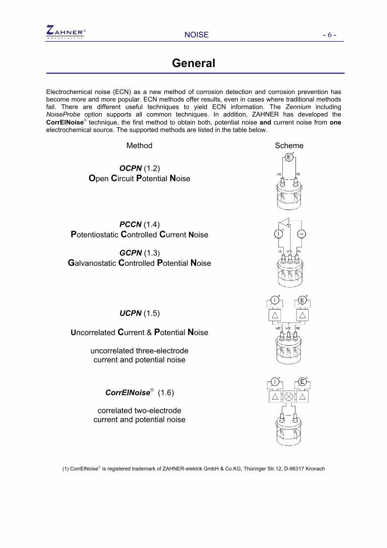
General Electrochemical noise (ECN) as a new method of corrosion detection and corrosion prevention has become more and more popular. ECN methods offer results, even in cases where traditional methods fail. There are different useful techniques to yield ECN information. The Zennium including NoiseProbe option supports all common techniques. In addition, ZAHNER has developed the CorrElNoise® technique, the first method to obtain both, potential noise and current noise from one electrochemical source. The supported methods are listed in the table below.

Method Scheme

OCPN (1.2) Open Circuit Potential Noise

PCCN (1.4) Potentiostatic Controlled Current Noise

GCPN (1.3)

Galvanostatic Controlled Potential Noise

UCPN (1.5)

Uncorrelated Current & Potential Noise

uncorrelated three-electrode current and potential noise

CorrElNoise® (1.6)

correlated two-electrode current and potential noise

(1) CorrElNoise® is registered trademark of ZAHNER-elektrik GmbH & Co.KG, Thüringer Str.12, D-96317 Kronach

NOISE - 7 -

CorrElNoise® - ( Correlated Electrochemical Noise ) Noise-based corrosion research using conventional electrochemical methods focuses on the fact that the initial redox processes are related to the charge transfer of the metal dissolution/deposition processes. Distinct areas of the object surface can be considered as local galvanic elements which contribute to the total potential measured. Since many of these local elements are superimposed, the fluctuation of the potential ( and the current, if the electrode is polarized ) is low. Traditional electrochemical methods base on this 'steady-state' behavior. However, inhomogeneous corrosion attack, which is particularly important in the nucleation phase, does not conform to these conditions. Traditional methods, such as the impedance or Tafel techniques fail when the measured signals become noisy, caused e.g. by the discrete nature of inhomogeneous corroding objects. In this case, noise measurements quantify these discrete events which are disturbing the continuous methods. Under the aspects of analysis, it is important to measure sizes, current noise as well as potential noise. The problem is that the measurement of current noise essentially requires a short-circuit condition, whereas potential noise must be measured with a high impedance load. The standard method for solving this problem is to measure two 'identical' systems, one under an open circuit, the other one under short-circuit conditions. A common experimental arrangement uses three identical electrodes, with one pair acting as a current noise source under short circuit-condition, the second one acting as a potential noise source under open circuit conditions. The third electrode acts as a common electrode. This arrangement is often used in monitoring applications. However, this method has a significant disadvantage when considering the fact that the measured current and the potential noise do not come from the same electrochemical system. Even though it is assumed that the corrosion behavior of the two systems is identical, current and potential are not correlated. This means that only the scalar rms values can be related, and vector operations like the power calculation are meaningless There is a solution for the problem, based on the fact that corrosion-related noise is mainly observed in the low frequency range. In a first approximation, the noise source can be described as a low frequency noise oscillator in series with a source resistance. Therefore, it is possible to sample current and potential signals by rapid switching between the two modes (open circuit and short circuit). If the switching and sampling frequency is high, relative to the highest relevant noise frequency, this technique will work without loss of information. CorrElNoise® stands for the measurement of correlated electrochemical current and potential noise coming form the same source. It enables the user to record current noise, potential noise and noise power in the frequency range from DC up to 5Hz. Moreover, CorrElNoise® benefits from the chopper principle. This means that

NOISE - 8 - electronic offset and drift problems, as well as line frequency interferences are automatically suppressed

Principle of the CorrElNoise® technique As the acquisition time of noise measurements is normally very long, there is a lot of data to be handled. The NOISE software allows to save measurement data in two ways. Generally, the software reduces the flood of data by a factor of 256. Then, access is given to the analysis mode used the most often, namely the frequency spectrum of the noise signal. The signal of the time domain can also be saved, so that any analysis method can be applied.

NOISE - 9 -

NOISE measurement

1. Measurement Main Menu NOISE starts up with a graphic menu including a set of buttons which can be activated by the user. Each of the buttons represents a submenu or an i/o function to select options or to define parameters.

NOISE - 10 -

2. Mode of Operation

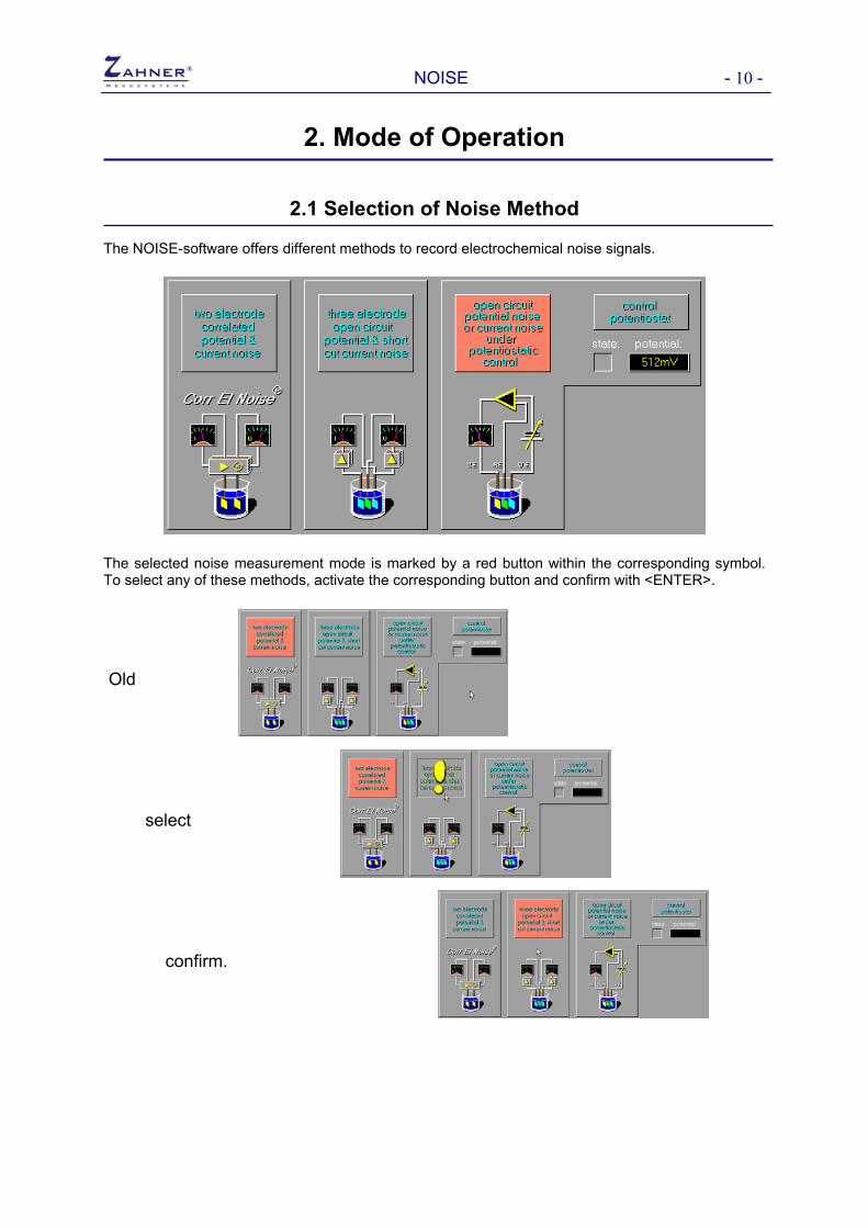
2.1 Selection of Noise Method The NOISE-software offers different methods to record electrochemical noise signals.

The selected noise measurement mode is marked by a red button within the corresponding symbol. To select any of these methods, activate the corresponding button and confirm with <ENTER>.

Old

select

confirm.

NOISE - 11 -

2.2 Control of Potentiostat

Activate the command <control potentiostat> of the EIS submenu 'test sampling & potentiostat control' to verify and change the settings of the potentiostat. If the potentiostat/galvanostat is <ON>, this will be indicated by the red ´state´ LED. The operating mode and the controlled DC parameter are given in two windows being named ´potential´ resp. ´current´.

The graphical window shown above appears when the ´test-sampling´ menu has been activated. This is the common menu to set the control parameters of the potentiostat/galvanostat. In the case of NOISE measurements, only the DC parameters are relevant. AC settings can be changed but will not affect the measuring conditions. On the left, four 'digital instruments' which indicate the measured and calculated parameters, have been installed. Four scopes on the lower right have been provided to show the perturbation signals of AC potential and AC current in the time domain as well as in the frequency domain. The scopes are not active during NOISE measurements. The set of buttons allows selective changes of the measuring parameters, including the main switch ON/OFF.

NOISE - 12 -

2.2.1 The Instruments - Measuring Parameters

The measured DC potential between the testing electrode sense and the reference electrode

!Note: Electrochemical diction „The reference potential is virtually zero“.

The measured DC current flowing from the counter electrode to test electrode

!Note: Electrochemical diction „Positive means anodic, negative means cathodic with respect to the working electrode“.

The modulus of the measured impedance. Inactive in NOISE.

The measured phase angle between AC voltage and AC current.

Inactive in NOISE.

2.2.2 Control Parameters & Mode Settings

'frequency' Not active during NOISE

'amplitude' Not active during NOISE

'count' Not active during NOISE

'POTENTIOSTAT / GALVANOSTAT' Two toggle switches are used to select the operating mode of the potentiostat. To select the potentiostatic mode, toggle ´POTENTIOSTAT´ To select the galvanostatic mode, toggle ´GALVANOSTAT´. When selecting a new operating mode, the potentiostat is switched off automatically due to reasons of security.

'potential / current' Toggling the 'potential' switch opens an input box where a new DC-parameter can be entered.

NOISE - 13 -

The main switches 'ON' and 'OFF'

The ´ON´ button is toggled to connect the pontentiostat with the measured object. The ´OFF´ button is toggled to disconnect the potentiostat from the i/o terminals.

Switching on the potentiostat will cause the following action: a) 'POTENTIOSTAT' The defined DC-voltage will be applied to the measured object. DC-

voltage and DC-current will be measured and displayed. The DC-voltage will be regulated and fixed, the DC-current will depend on the measured object only.

b) 'GALVANOSTAT' Within the potentiostatic limits the potentiostat will apply the defined DC-current to the measured system and compensate fluctuations. The output voltage of the potentiostat cannot be affected by the user. The measured potential and the measured current will be put out.

NOISE - 14 -

2.3 OCPN Open Circuit Potential Noise

OCPN measures the potential noise of an open circuit cell. The sensitivity of this noise method is relatively low. Furthermore no information about the current noise can be obtained.

! NOTE!

To set up OCPN the potentiostat must be switched <OFF>. Connecting the cell to an active potentiostat might cause uncontrolled stress to the system or severe damage of the hardware.

When the potentiostat has been switched <OFF> the cell will be connected to the potentiostat or to the noise probe as shown below.

NOISE - 15 -

2.4 GCPN Galvanostatic Controlled Potential Noise

GCPN measures the potential noise at a controlled cell current. The sensitivity of this noise method is relatively low when the main potentiostat is the selected device. No information about the current noise will be obtained.

! NOTE!

To set up OCPN the potentiostat must be switched <OFF>. Connecting the cell to an active potentiostat might cause uncontrolled stress to the system or severe damage of the hardware.

When the potentiostat has been switched <OFF> the cell will be connected to the potentiostat or to the noise probe as shown below.

To set up the current activate the potentiostat control menu. Select operational mode <GALVANOSTAT>, set the current and switch <ON> the galvanostat. Finally return to the noise program by use of the <HOME>-function.

NOISE - 16 -

2.5 PCCN Potential Controlled Current Noise

PCCN measures the current noise at a defined cell potential. The sensitivity of this noise method is relatively low. No information about the potential noise can be obtained.

! NOTE!

To set up PCCN the potentiostat must be switched <OFF>. Connecting the cell to an active potentiostat might cause uncontrolled stress to the system or severe damage of the hardware.

When the potentiostat has been switched <OFF> the cell will be connected to the potentiostat or to the noise probe as shown below.

To set up the potential activate the potentiostat control menu. Select operational mode <POTENTIOSTAT>, set the potential and switch <ON> the potentiostat. Finally return to the noise program by use of the <HOME>-function.

NOISE - 17 -

2.6 UCPN Uncorrelated three electrode Current and Potential

Noise

UCPN will be measured in a three electrode setup.

! NOTE!

To set up UCPN the potentiostat must be switched <OFF>. Connecting the cell to an active potentiostat might cause uncontrolled stress to the system or severe damage of the hardware.

To measure uncorrelated current and potential noise the NProbe must be used. The use of the NProbe offers selective use of DC-coupling or AC-coupling of the measured signals. To select DC-coupling or AC-coupling use the toggle switch within the selective button of the UCPN symbol.

2.6.1 Noise Probe & DC-Coupling Using DC-coupling and the noise probe does not affect the resolution of the measured signal. The overall signal will be measured with a resolution of 20-bit and offers a relatively high resolution of small AC-signals which are superimposed to a DC-component of high level (e.g. DC-range=2V, AC-resolution=2uV/bit). By using the <offset>-option the resolution of the realtime display may be increased. The use of the <offset>-option does not affect the measuring technique and the resolution of the measured data.

2.6.2 Noise Probe & AC-Coupling Measuring noise signals of very low amplitude the AC-coupling mode of the noise probe should be selected. This will result in a very high resolution of the measured signal down to 100nV/bit. Furthermore the active filtering provides a selective bandwidth limiting of the measured signals. However, the information of the DC-component will be lost.

When the potentiostat has been switched <OFF> the cell will be connected to the noise probe as shown below.

NOISE - 18 -

2.7 CorrElNoise®

Correlated two electrode Current and Potential Noise

CorrElNoise® is highly sensitive to current and potential noise signals. In contrast to the methods described above CorrElNoise® does work in the DC-coupled mode only. To avoid high DC-levels of the measured signals symmetrical systems should be used, i.e. both electrodes should be of the same material. By the unique generation of correlated signals of both potential and current from one electrochemical source additional magnitudes like noise power or impedance can be calculated. CorrElNoise® will be measured in a two electrode setup.

! NOTE!

To measure CorrElNoise® the potentiostat must be switched <OFF>. Connecting the cell to an active potentiostat might cause uncontrolled stress to the system or severe damage of the hardware.

When the potentiostat has been switched <OFF> the cell will be connected to the potentiostat or to the noise probe as shown below.

NOISE - 19 -

3. Noise Recording Control Parameters

3.1 Alert Count

During noise measurements the recorded signals will be checked by means of control conditions. If any of these conditions will be violated an 'alert' will be generated. These alerts will be stored and displayed within the realtime screen.

NOISE offers four different kinds of alerts:

3.1.1 Pink Noise

The actual time spectrum(spectra) Y(t) will be

transformed by means of a zoom-fft. The -value(s) and the amplitude squares

will be calculated. Finally the resulting curve(s) rmsY )(2

0 fY2Y

over log(f) will be investigated by means of linear regression.

A 'pink noise' alert will be given if a) the slope m of the regression line will exceed 1 ( 1>m , here 1−<m ) and if b) the rms value will exceed the defined limit.

NOISE - 20 -

3.1.2 Correlation

The recorded time signal will be compared with a reference time signal. If the calculated coefficient of correlation will exceed the set value a 'correlation' alert will be given.

3.1.3 Standard Deviation

( )2

1∑ −=

N

m YYS

Within one block the standard deviation of the measured data will be calculated. If the standard deviation will exceed a defined limit a 'standard deviation' alert will be registrated.

3.1.4 RMS-Overflow

After a block has been recorded the measured time spectra will be Fourier transformed and the scalar rms-values ( , , ) will be calculated. If one of these values will exceed the set limit an alert counter will be incremented

rmsE rmsI )1(rmsN

dtYT

RMS ∫= 21

eCorrElNoiscase)1( ®

3.2 Weighting List

The 'weighting list' offers manipulation of the rms-calculation by the user. This list will be stored in a vector w(n) of dimension n of the Fourier transforms. During rms-calculation the Fourier transforms will be convoluted with this vector. By default the weighting vector w() is a unity vector containing 1s.

To select a certain frequency interval for rms calculation the weighting list may be altered, e.g.: The frequency range 500mHz<=f<=2Hz is of special interest. Therefore this range should be weighted with 1, all other frequencies shall be neglected. To redefine the weighting list activate the list editor and set all weighting factors out of the frequency range equal zero.

NOISE - 21 - To select any factor move the cursor by use of the <↑>- and <↓>-keys and put in the new factor at the chosen frequency. The weighting factors may be changed in the valid range 0<=WFac<=1.

After all changes have been done the new list may be saved.

To leave the list editor use the <HOME>-function.

NOTE! There is only one weighting list. After startup of the program the weighting vector will be the unity vector. When activating 'weighting' in the main menu, the stored list will be loaded.

3.3 Auto-Ranging

Activating the 'auto-ranging'-option the amplification factors of both, hardware and software, will be changed automatically when exceeding the limits.

3.4 Offset

The offset option offers DC corrections of the measured signal to obtain the highest possible resolution of the small amplitude noise signals.

3.4.1 Software Offset Correction Using the offset option (ON) the program will subtract a certain DC potential from the incoming signals. This will result in a higher resolution of the displayed data. In the continuous mode this offset will be set to the last measured value of the last sequence having been recorded. Using the offset option as toggle (ON-OFF or OFF-ON) the last measured value will be the next offset value.

NOISE - 22 -

-200

noise before offset noise after offset

offset

10

0

-10

200

0

200

0

3.4.2 Hardware Offset Correction Using the internal potentiostat of the Zennium the offset will be subtracted from the incoming signals by hardware. Considering the 100times lower resolution of the Zennium in comparison to the noise probe the analyzer may be forced to use a higher shunt resistor. This will increase the dynamic resolution of the measurement. Hardware offset correction has not been included to the noise probe.

sample &hold

inputsignal

offset

toanalyser

3.5 Frequency range

By 'frequency range' two recording parameters will be defined.

NOISE - 23 -

3.5.1 The Investigated Frequency Range The frequency range of the frequency domain data spans three decades and will be defined by setting the upper limit fmax of the interval.

Upper Limit (1,2,5,...,fmax) Case fmax / Hz

CorrElNoise® 10 NProbe 20 Zennium The defined frequency scale of the frequency domain will be split into 60 values f equidistant in log(f).

3.5.2 Noise Data Recording Window The time domain acquisition will be separated into blocks. After a block has been recorded Fourier transforms, RMS-values, trend values, alerts, etc. will be calculated. Further on data will be stored block oriented. Every time a block has been finished data will be reduced and stored to file if the 'saving'-option has been activated.

100

The length of a block is given by the reciprocal of the lowest frequency of the frequency range: tblock = fmin

-1

This time interval will be equivalent to 2048 data points. In order to suppress side effects caused by discretization of time intervals, a so called Hanning window weights the time domain data by means of an 1+cos(t) characteristic. The “windowed” time interval consists of two consecutive blocks with 4096 samples total, and it is moved over the time axis every 2048 sample counts. By this strategy every analyzed data block overlaps 50% with the previous one and artifacts caused by discrete rectangular windows are avoided. The discrete Fourier analysis (FFT) delivers then 2048 complex frequency

samples in frequency steps of blockt

f⋅

=Δ2

1. The convolution with the cosine window suppresses the

first harmonic (it contains now DC component information), and the 2nd harmonic is identical with the fundamental of the 2048-block time transform. Note, that the following harmonics 3…2047 correspond to frequency steps of 1.5, 2, 2.5… referred to a 2048-block time transform. In the ASCII text export list the details, sketched in the table below, are listed.

NOISE - 24 -

Note: if saving is activated, time domain records are stored on the settings state; calculated frequency domain results are always stored. In order to obtain sufficient data reduction for long term recording, the 2048 frequency lines are compressed into a coarse logarithmic distribution of 60 averaged ones. Harmonic order# content

of the total transform Count of lines / bandwidth

weighting factor Effective frequency relative to the

analyzed time domain block 0 na DC component / 2 1 na DC component / 2 2 1 Fundamental fmin

1.5 fmin3 1 2 fmin4 1

2.5 fmin – 9.5 fmin5…19 1 10 fmin – 22.5 fmin20-23; 24-30; 31-38; 39-49 2; 3; 4; 5 25.25 fmin – 40 fmin26, 27; 28, 29; 30; 31,32 6; 7; 8; 9

…. .... 44.725 fmin – 984 fmin

NOISE - 25 -

4. Start Measurement

NOISE ® offers two kinds of realtime display during a measurement

• time domain measurements

and

• frequency domain measurements.

These methods differ in the kind of realtime display and in the format noise data will be stored. However, the methods do not differ in the mode of data recording. Maximum flexibility is needed to process data in both time and frequency domain. Only a little data reduction should be done in order to avoid any loss of information. This has been realized by the real time acquisition mode. The time course of potential and/or current is sampled with 8-fold oversampling. The signal will be limited in bandwidth online by a FIR-filter which is responsible for an 8-fold reduction of the oversampled data. This reduced data stream is stored on harddisc in blocks of 2048 16-bit-words per channel. The time course will not be interrupted during acquisition. The length of one block is defined by the reciprocal of the lowest frequency of the frequency domain window (<frequency range>).

NOISE - 26 -

4.1 Time Domain Measurements

The time domain measurement window will be dominated by the data window. Several switches and buttons have been installed to modify parameters during recording. After the measurement has been started no data will be saved. When the optimal recording parameters - potential range, current range and offset - have been set and the system will have settled, data saving may be activated.

4.1.1 Potential Scaling & Activation

A set of buttons offers adaption of the potential resolution of both software and hardware. Within the realtime window the full scale limit will be given. Further on a toggle switch offers selection of display and storage of potential data.

NOISE - 27 -

activate/deactivate potential recording

increase sensitivity

decrease sensitivity

4.1.2 Current Scaling & Activation

A set of buttons offers adaption of the current resolution of both software and hardware. Within the real . Further on a toggle switch offers selection

time window the full scale limit will be given of display and storage of current data.

increase sensitivity

decrease sensitivity

activate/deactivate current recording

4.1.3 Time Scaling

he full scale factor of the time scale will be set. T

enlarge time scale

redu

ce time scale

tion 4.1.4 Ranging Op

'ranging' works as toggle switch. In the active mode the full scale factor will be increased automatica al limits.

lly if data will exceed the actu

4.1.5 Offset Option

'offset' works as toggle switch. In the active mode ranging may be avoided by offset corrections. A new of fter a block measurement has been finished.

fset will be calculated a

4.1.6 Saving Option

By activation of 'saving' a new data file will be generated to store noise data. After a block measurement th ed to the actual file. Deactivation of 'saving' will end data storage.

e new block will be append

NOISE - 28 -

4.1.7 Hardcopy

A hardcopy of the actual data window may be put out to a printer. Activating 'hardcopy' will interrupt the measurement.

The displayed data may be put out via the lineprinter hardcopy function. Before output a menu will offer the setting of the print parameters. Thus the size of the hardcopy and its orientation can be

cted to certain requirements.

• big (landscape) t)

Fina t may be started and a form feed may be enforced.

sele

• to clipboard • save as file • HCOPY

• small (uprigh

lly he output

NOISE - 29 -

4.2 Frequency Domain Measurements

The frequency domain measurement window will be dominated by the data window. Several switches and buttons have been installed to modify parameters during recording. After the measurement has been started no data will be saved. When the optimal recording parameters - potential range, current range and offset, etc. - have been set and the system will have settled, data saving may be activated.

4.2.1 Potential Scaling & Activation

A set of buttons offers adaption of the potential resolution of the display software. Further on a toggle switch offers selection of display and storage of potential data.

NOISE - 30 -

decrease sensitivity

increase sensitivity

activate/deactivate potential recording

4.2.2 Current Scaling & Activation

A set of buttons offers adaption of the current resolution of the display software. Further on a toggle switch offers selection of display and storage of current data.

decrease sensitivity

increase sensitivity

activate/deactivate current recording

4.2.3 Time Scaling

The full scale factor of the time scale will be set.

enlarge reduce

time scale time scale

4.2.4 Ranging Option

'ranging' works as toggle switch. In the active mode the full scale factor of the display will be ranged automatically.

4.2.5 Offset Option

'offset' works as toggle switch. In the active mode ranging may be avoided by offset corrections. A new offset will be calculated after a block measurement has been finished.

4.2.6 Saving Option

By activation of 'saving' a new data file will be generated to store noise data. After a block measurement the new block will be appended to the actual file. Deactivation of 'saving' will end data storage.

NOISE - 31 -

4.2.7 Hardcopy

A hardcopy of the actual data window may be put out to a printer. Activating 'hardcopy' will interrupt the measurement.

The displayed data may be put out via the line printer hardcopy function. Before output a menu will offer the setting of the print parameters. Thus the size of the hardcopy and its orientation can be selected to certain requirements.

• to clipboard • save as file • HCOPY • big (landscape) • small (upright)

A hardcopy of the actual data window may be put out to a printer. Activating 'hardcopy' will interrupt the measurement.

NOISE - 32 -

5. Noise - Analysis

The NOISE® analysis software is activated up by pressing this button. The actual data will not be present at the very moment. Due to reasons of safety recorded data should first be saved in the recording program, then that measure data may be loaded by the analysis program.

6. Noise Data File Operations

The button 'file operations' leads to a submenu offering disc-i/o-operations.

The options ´save´ and ´load´ will activate the WINDOWS® file browser.

NOISE - 33 -

6.1 Setup of Hardware for Electrochemical Noise Measurements

6.1.1 Connecting the Noise Probe to the Zennium The noise probe will be controlled by the Zennium via the EPC4/40-controller module. To set up the noise probe connect the LEMOSA 8-pin plug to any of the 4 terminals of the EPC-module. To address the noise probe select the corresponding terminal's number in the submenu <test sampling> by activating the button named <DEVICE> and put in the terminal's number. After the selection has been confirmed the active device name will be NoisePx, where x indicates the selected channel.

IM6 EPC40

4

3

2

1

Cell

EPC

40

Cor

rElN

oise

-

tech

nolo

gy

™

NP

ER

OB

6.1.2 Connecting the Cell to the Noise Probe The noise probe will be delivered with two sets of cables: CABLE1 has three lines and will be used during CorrElNoise® measurement. CABLE2 has four lines and must be used in standard noise measurements or when the noise probe is used as external potentiostat/galvanostat NOTE:

Floating and ground referenced objects demand different connections to the potentiostat. Use the integrated switch in the 9-pin sub-D-plug to select

1 floating object 1

00 any type of ground connection

NOISE - 34 -

6.2 CorrElNoise®

Use cable 1 and connect the cell as shown below. Connect the green plug to one electrode and connect the blue plug to the second electrode. The black plug will be connected to the shield of the cell. Due to the small signals shielding should always be used to avoid external noise pick up by e.g. 'electro smog'.

CorrElNoise

E2E1

shie

ld

CABLE1

6.3 Using the Noise Probe as External Potentiostat/Galvanostat The colored plugs correspond to the colors of the main potentiostat of the Zennium. Use CABLE2 for potentiostatic/galvanostatic measurements. red counter electrode green reference electrode black working electrode power blue working electrode sense

E3 E2E1

RECE WE

shie

ld

CABLE2

To run potentiostatic/galvanostatic measurements refer to the connection schemes of the main potentiostat being described in the EIS-section of the manual.

NOISE - 35 -

6.4 Standard Noise Measurements

6.4.1 Open Circuit Potential Noise OCPN Use CABLE2 and connect as shown right. The active electrodes are WEs working electrode sense -> E1 RE reference electrode -> E2 WE working electrode -> shield CE counter electrode not connected

E2E1

WEs REsh

ield

donotconnect

CABLE2

6.4.2 Galvanostatic Controlled Potential Noise GCPN Use CABLE2 and connect as shown right. The active electrodes are WEs working electrode sense -> E1 RE reference electrode -> E3 WE working electrode -> shield CE counter electrode -> E2

E3 E2E1

REWEs CE

shie

ld

CABLE2

NOISE - 36 -

6.4.3 Potentiostatic Controlled Current Noise PCCN Use CABLE2 and connect as shown right. The active electrodes are WEs working electrode sense -> E1 RE reference electrode -> E3 WE working electrode -> shield CE counter electrode -> E2

E3 E2E1

REWEs CE

shie

ld

CABLE2

6.4.4 Uncorrelated Current & Potential Noise UCPN Use CABLE2 and connect as shown right. The active electrodes are WEs working electrode sense -> E2 RE reference electrode -> E1 WE working electrode -> E3 CE counter electrode not connected

E3 E2E1

WERE WEs

donotconnectCABLE2

NOISE - 37 -

NOISE analysis

7. Analysis Main Menu

The NOISE analysis starts with a graphic menu including a set of buttons which can be activated by the user. Each of the buttons represents a submenu or an i/o function to select options or to define parameters.

After the start-up of the program all display options will be reset t default settings and all output channels ( = measured magnitudes ) will be deactivated. The state of an output channel or of a display option will be indicated by a symbolic LED, i.e. green = on / active, red = off / passive.

NOISE - 38 -

8. File Operations

The button <file operations> will activate the WINDOWS file browser. The saving option, however, has been disabled. After a noise measurement has been loaded the following parameter of the measurement will be displayed at the left of the output window.

8.1 Present File's Name

The file name of the noise measurement being loaded last will be indicated within the output box named {present file's name}.

8.2 Time Window

After loading a noise measurement the recording window of the data will be indicated: e.g. starting time ts = 11:00:02 recording time te = 11:30:02 duration td = 00:30:00. The time window may further on be used to zoom the time scale. By this option certain sections of the measured data can be selected for detailed studies.

! NOTE!

To obtain frequency domain diagrams the minimal width of the time window must at least be selected double as long as the reciprocal of the lowest frequency having been measured.

e.g.: fmin = 100mHz --> dtmin = sec20100

1=⋅

mHz2

tmin tmax

0 20 10 30 ... ...

8.3 Display Protocol

The file name of the noise measurement being loaded last will be indicated within the output box named {present file's name}.

The noise data files' header block will be displayed

NOISE - 39 -

.

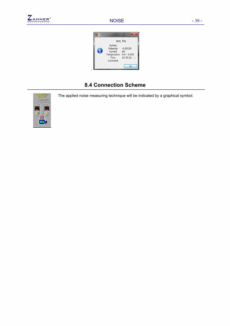
8.4 Connection Scheme

The applied noise measuring technique will be indicated by a graphical symbol.

NOISE - 40 -

9. Display Parameter The NOISE® analysis software offers different types of diagrams for the display of noise data. The different types of display may be activated parallel and can be plotted within one diagram. The corresponding buttons will be found at the top of the output window.

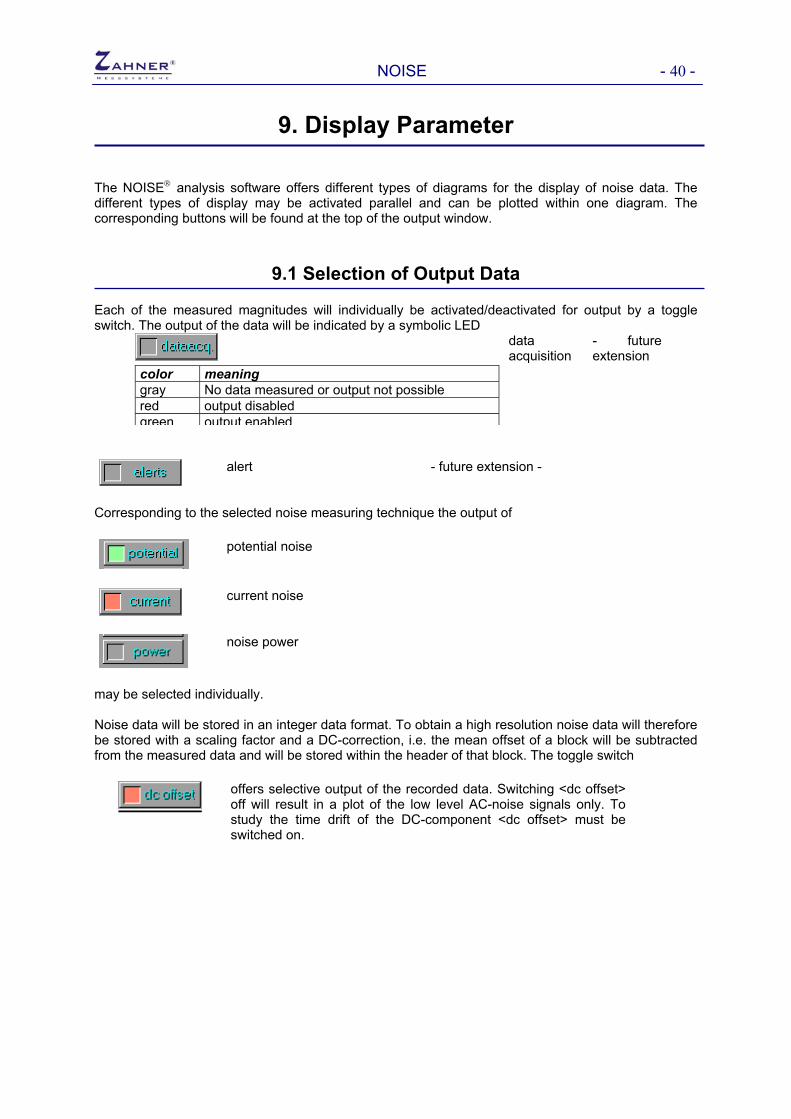
9.1 Selection of Output Data Each of the measured magnitudes will individually be activated/deactivated for output by a toggle switch. The output of the data will be indicated by a symbolic LED

data acquisition

- future extension

color meaning gray No data measured or output not possible red output disabled green output enabled

alert - future extension -

Corresponding to the selected noise measuring technique the output of

potential noise

current noise

noise power

may be selected individually. Noise data will be stored in an integer data format. To obtain a high resolution noise data will therefore be stored with a scaling factor and a DC-correction, i.e. the mean offset of a block will be subtracted from the measured data and will be stored within the header of that block. The toggle switch

offers selective output of the recorded data. Switching <dc offset> off will result in a plot of the low level AC-noise signals only. To study the time drift of the DC-component <dc offset> must be switched on.

NOISE - 41 -

9.2 Selection & Activation of Diagram Types Three types of diagrams will be offered by the noise analysis program:

time domain diagram

frequency domain diagram

trend analysis

Each of the buttons will activate a pop-up menu to select different types of anaylsis and to activate/deactivate the output of the corresponding data. The output of the analysis' data will be indicated by a symbolic LED within the button (green = output of diagram, red =no output of diagram).

9.3 Time Domain Diagram

Time domain diagrams can be printed out automatically <auto> or manually <man>. The additional toggle switch, <diagram active> allows selective output of the time domain diagram.

Automatic scaling is selected by pressing the button.

Manual scaling is selected with the button.

Toggling the switch <diagram active> enables or disables the output of time domain diagrams.

9.4 Frequency Domain Diagram (FFT)

Selection and parameter settings of the frequency domain representation are carried out in the submenu 'frequency domain'. Frequency domain spectra are obtained by a Fourier transform of the time domain data. Different magnitudes of the Fourier spectra can be selected

9.4.1 Selection of the Magnitude The output of the Fourier amplitudes A(f) will be selected here.

! NOTE!

The selection of <lin. amplitude> will offer both, 2d and 3d display. At the moment, however, only the 3d diagram will be put out regardless of the selection of the diagram type.

NOISE - 42 -

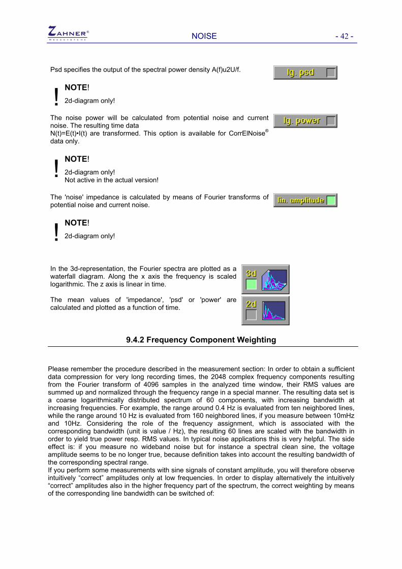
Psd specifies the output of the spectral power density A(f)u2U/f.

! NOTE!

2d-diagram only!

The noise power will be calculated from potential noise and current noise. The resulting time data N(t)=E(t)•I(t) are transformed. This option is available for CorrElNoise® data only.

! NOTE!

2d-diagram only! Not active in the actual version!

The 'noise' impedance is calculated by means of Fourier transforms of potential noise and current noise.

! NOTE!

2d-diagram only!

In the 3d-representation, the Fourier spectra are plotted as a waterfall diagram. Along the x axis the frequency is scaled logarithmic. The z axis is linear in time. The mean values of 'impedance', 'psd' or 'power' are calculated and plotted as a function of time.

9.4.2 Frequency Component Weighting Please remember the procedure described in the measurement section: In order to obtain a sufficient data compression for very long recording times, the 2048 complex frequency components resulting from the Fourier transform of 4096 samples in the analyzed time window, their RMS values are summed up and normalized through the frequency range in a special manner. The resulting data set is a coarse logarithmically distributed spectrum of 60 components, with increasing bandwidth at increasing frequencies. For example, the range around 0.4 Hz is evaluated from ten neighbored lines, while the range around 10 Hz is evaluated from 160 neighbored lines, if you measure between 10mHz and 10Hz. Considering the role of the frequency assignment, which is associated with the corresponding bandwidth (unit is value / Hz), the resulting 60 lines are scaled with the bandwidth in order to yield true power resp. RMS values. In typical noise applications this is very helpful. The side effect is: if you measure no wideband noise but for instance a spectral clean sine, the voltage amplitude seems to be no longer true, because definition takes into account the resulting bandwidth of the corresponding spectral range. If you perform some measurements with sine signals of constant amplitude, you will therefore observe intuitively “correct” amplitudes only at low frequencies. In order to display alternatively the intuitively “correct” amplitudes also in the higher frequency part of the spectrum, the correct weighting by means of the corresponding line bandwidth can be switched of:

NOISE - 43 - Frequency component weighting in wideband mode In the true RMS/power mode, measuring a clean sine 2 Hz between 20mHz and 20Hz of 100mV amplitude is “intuitively” wrong displayed here as about 20mV.

Frequency component weighting in wideband mode switched off: Measuring a clean sine of 2Hz between 20mHz and 20Hz of 100mV amplitude is here displayed “intuitively” correct. Please consider that this setting ignores the natural spectral unit of value / Hz of the data and PSD and RMS/power spectra can now no longer be correct. Use this mode only for orientation, when you apply sine waves.

9.4.3 Diagram Type The frequency domain data can be displayed by two diagram types. Selection of one of the magnitudes 'lg. psd','lg. power','lg. impedance' releases the previous setting and the 2d-diagram mode will be activated. Only 'lin. amplitude' data may be plotted in a 3d-plot. The output of the frequency domain diagram is selected with the toggle switch named <diagram active>. Toggling this switch enables or disables the output of the frequency domain diagram.

NOISE - 44 -

9.5 Trend Analysis

The trend of potential noise, current noise and noise power can be analyzed by the calculation of the rms value or the standard deviation.

Selection and scaling modes of these magnitudes are offered by the trend analysis menu. The output of the standard deviation is selected by this button.

Here, the rms calculation is selected.

- to be extended in the future -

On the right of each selective switch, a toggle switch offers either automatic or manual scaling of the corresponding data. The output of the trend diagram is selected with the toggle switch named <diagram active>. Toggling this switch enables or disables the output of the trend diagram.

NOISE - 45 -

10. Display Diagram

Pressing the <display>-button will create a new drawing. A set of three graphic symbols to the left of the data window offer different export functions.

NOISE - 46 -

10.1 Export Data

According to the import rules of different analysis programs, the present data are stored as formatted files. A standard ASCII-list will be exported, which can be imported by any program offering an ASCII input interface.

NOISE supports the following formats Data will directly be stored to the MS-DOS device being named within the save dialog box. Considering time domain data the creation of the file may take a long time. We do not recommend the storage on a floppy disc as the file length may soon exceed some megabyte. Passes an ASCII list on to the THALES interfaces directly to the TAHLES Editor „ZEdit“.

! NOTE!

Time domain data should be exported by using time windows of reduced length. ASCII-export requires both, patience by the user and a BASIC-stack being large enough to pass the data from one program to the other. Export of long measurements in one block may cause the system to crash.

10.2 Hardcopy

A hardcopy of the actual data window can be put out on the windows standard printer or can be copied to clipboard as a bitmap. Before output is effected, a menu offers the setting of the print parameters: <settings> toggles between output modes

• to clipboard • save as file • HCOPY

• big (landscape) • small (upright)

<form feed> enables to enforce a form feed for output <output> starts the output with actual settings

10.3 Export Drawing

The actual graphics are passed on to the THALES program CAD. The created graphics can be altered and saved as a HPGL™ file, which can directly be imported to other programs, such as Word®, CorelDraw® or Page-Maker® ™ and all other programs with an HPGL import filter.

! NOTE! The export of time domain data to an HPGL-formatted list will require some patience by the user. To give an estimation: the export of 10 blocks of one magnitude - potential or current - will at least effort 60 seconds of time.