Noise reduction procedures for gravity-gradiometer data

Mark Pilkington1 and Pejman Shamsipour1

ABSTRACT

Noise suppression of airborne gravity-gradiometer data isa crucial part of the data processing stream. We consideredtwo approaches to removing noise: kriging and directionalfiltering. Kriging is an estimation procedure for the interpo-lation of spatial data. The estimator is calculated from thedata variogram, which characterizes the noise level and cor-relation length of the measurements. Directional filteringuses a user-defined operator that is oriented to preferentiallysmooth the data along the strike, but it leaves short-wave-length components in the cross-strike direction for definitionof the trend edges. Both methods were applied to a recentlycollected offshore gravity gradient survey. The kriging anddirectional filtering results revealed a similar level ofsmoothness, but the main difference between them wasthe extra smoothing along the strike for the directionally fil-tered data. Because kriging is a data-driven procedure, itprovides an objective estimate of the data noise level anddegree of smoothness. The processing parameters requiredfor directional filtering can then be chosen to give a similarlevel of smoothness and noise suppression to the kriging re-sults, but with the added advantage of directional smoothing,which more effectively delineates geologic trends in thedata.

INTRODUCTION

Ongoing improvements in gravity gradiometry technology haveled to its establishment as a powerful technique in mining and hy-drocarbon exploration. In addition to providing high-resolutiongravity data, the availability of the gravity gradient tensor offers, incomparison with the vertical gravity component, a much richer sig-nal with increased options for processing and interpretation meth-ods. Any such methodologies must address the possibility of noisein the data and include appropriate steps to mitigate the unwanted

effects of a noisy signal. This is the focus of this study, the suppres-sion of noise in gravity-gradiometer data.The sources and approaches to treatment of noise in airborne

gravity-gradiometer (AGG) systems are numerous and have beendiscussed extensively in the literature (Hammond and Murphy,2003; Boggs and Dransfield, 2004; Barnes and Lumley, 2011; Di-Francesco, 2013; Dransfield and Christensen, 2013). Certain noisesources are related to the AGG instruments, e.g., measurement errorand noise induced by aircraft turbulence. Other sources arise fromthe subsequent processing of data, as in terrain correction errors andartifacts introduced from leveling and gridding operations. Standardprocessing of AGG data is designed to suppress the unwanted noiseand emphasize the geologic signals present. With continuing im-provements in survey design and operation and data processingmethods, predicted noise levels are expected to decrease furtherin the future (DiFrancesco, 2013). Nonetheless, currently producedAGG data often still contain high enough levels of noise to interferewith qualitative and quantitative interpretations. Our approach hereis to explore noise-reduction methods and determine their appli-cability and effectiveness in removing unwanted noise in AGG data.A major strength of gravity-gradiometer surveys is the high-

resolution content of data that can be achieved, particularly whencompared with airborne gravity surveys. Hence, any noise-removalapproach should preserve this key asset. But the most commonmethod to combat noise is to smooth or low-pass filter the data,which effectively degrades resolution. To avoid smoothing, Lyrioet al. (2004) use a wavelet-based approach, making the assumptionthat the signal and noise can be separated in the wavelet domain,once a suitable threshold scale is found. Denoised data are deter-mined by transforming back from the wavelet domain after theselected noise component contributions are set to zero. Theirapplication is applied only to line data, but it should be applicableto gridded data. Unlike frequency-domain filtering, the waveletmethod is spatially variant. Consequently, any smoothing donecan vary along with the noise properties, so that regions weaklyaffected by noise are not overly filtered, possibly removing a usefulgeologic signal. Therefore, the notion of spatially variant noise re-moval is one that we also adopt in this study.

Manuscript received by the Editor 19 February 2014; revised manuscript received 5 May 2014; published online 5 August 2014.1Geological Survey of Canada, Ottawa, Ontario, Canada. E-mail: mpilking@nrcan.gc.ca; pejman.shamsipour@polymtl.ca.© 2014 Society of Exploration Geophysicists. All rights reserved.

G69

GEOPHYSICS, VOL. 79, NO. 5 (SEPTEMBER-OCTOBER 2014); P. G69–G78, 13 FIGS.10.1190/GEO2014-0084.1

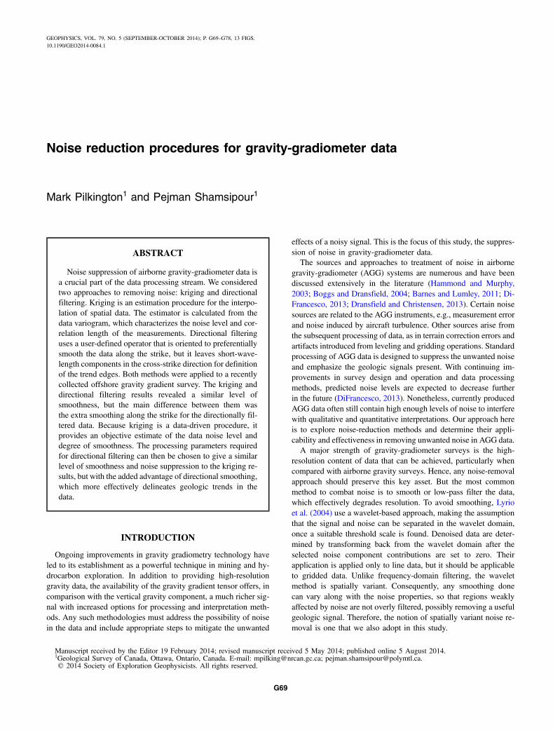
A key aspect of effective noise removal is to characterize thenoise properties and then design the noise-reduction method basedon this description. Studies of noise in AGG systems suggest thatthe noise can be assumed to be white, i.e., uncorrelated, with a flatpower spectrum (Dransfield and Christensen, 2013). Even thoughthis implies noise energy present at all wavelengths, the effects ofnoise are usually most pronounced at the shortest wavelengthspresent in the data. Most of the power in tensor component data(as with other potential field data) is concentrated in the long-wave-length portion of the spectrum, with a decrease in power as thewavelength decreases. Hence, noise is usually overwhelmed bythe geologic signal at longer wavelengths. This is generally the case,even if some correlation is present in the noise component, leadingto increased longer wavelength power. Processing of the raw mea-sured AGG data involves substantial low-pass filtering with a cut-off wavelength usually close to the line spacing distance. The actualvalue will also vary with the type of airborne platform used. Theeffect of the low-pass filtering is to emphasize the appearance ofany noise present at the cut-off wavelength, even if the noise ispresent at longer wavelengths. Figure 1 shows two examples ofAGG data collected over outcropping Precambrian shield rocksin Canada. Little geologic signal is apparent in the maps, which

are dominated by noise characterized by a wavelength of 250–500 m, corresponding to the cut-off wavelength range used inthe processing.In the following, we consider two approaches to noise removal

applied to AGG data: kriging and directional filtering. The data werefer to are those usually supplied by airborne survey contractors, inthe form of individual tensor component values. We assume thatthese data have undergone standard processing to account for meas-urement and dynamic errors and are also processed to be consistentwith Laplace’s equation through either the fast Fourier transform(FFT) (Sanchez et al., 2005), Fourier series (Yuan et al., 2013),or equivalent source (Li, 2001) methods.

KRIGING

Kriging is an estimation procedure commonly used in geostatis-tics for the interpolation of spatial data. The method is based on thetheory of regionalized variables (Matheron, 1963) and provides thebest linear unbiased estimator for a given problem. The basis of themethod is to find an estimator Z�

0 of some field from a set of neigh-boring field values ZðxiÞ ði ¼ 1; : : : ; nÞ. The field ZðxiÞ is assumedto be stationary with a constant average value and known covarianceCðhÞ. The estimator is constructed as follows:

Z�0 ¼

Xni¼1

λiZðxiÞ; (1)

where the unknown weights λi are to be determined. The estimatorZ�0 is unbiased, so the sum of the weights λi equals one. The weights

are a function of the distance between Z�0 and the surrounding ZðxiÞ,

with the closer points exerting more influence on the estimatedvalue than distant ones.Importantly, kriging incorporates the correlation between data

points into the estimator Z�0 through the variogram γðhÞ, given by

γðhÞ ¼ 1

2k

Xki¼1

½ZðxiÞ − ZðxiþhÞ�2; (2)

where k is the number of pairs of points that are separated by adistance h. If the field Z is a stationary process, then γðhÞ is inde-pendent of location and a single variogram can be used for process-ing the entire data set. As h increases to a value known as the range,γðhÞ levels off to a constant value (σ2). The variogram γðhÞ is re-lated to the covariance CðhÞ by

γðhÞ ¼ σ2 − CðhÞ; (3)

where σ2 is the process variance. The variogram may differ accord-ing to the direction considered, so that each h can be subdivided byorientation and anisotropic effects easily included.When modeling typically isotropic variograms, we need to define

three parameters: the range, sill, and nugget effect. The range is thedistance after which no more correlation exists between two obser-vations. The sill is the upper limit value of the variogram at a dis-tance equal to the range. If it exists, the sill represents the variance ofthe field. The nugget effect represents the combined effects of short-scale variation of the field, positioning errors, measurement inaccur-acy, and any variability of the field occurring at small enough scalesto be unresolved by the sampling interval. Therefore, it can be

0

2000

4000

6000

8000

Nor

thin

g (m

)

0 2000 4000 6000 8000Easting (m)

–35

–30

–25

–20

–15

–10

–5

0

5

10

15

20

25E

0

2000

4000

6000

8000

Nor

thin

g (m

)

–40

–35

–30

–25

–20

–15

–10

–5

0

5

10Ea)

b)

Figure 1. Two examples of noise in AGG data. (a) Data (Tzz) fromBlatchford Lake, Northwest Territories, collected at 250-m linespacing and 100-m mean flight height. The contour interval is5 E. (b) Data (Tzz) from McFaulds Lake, Ontario, collected at250-m line spacing and 100-m mean flight height. The contour in-terval is 5 E.

G70 Pilkington and Shamsipour

considered as the total residual random noise remaining in the dataafter initial processing.Once the variogram is calculated, the estimator Z�

0 is found byminimizing the error variance ðZ�

0 − Z0Þ2, leading to the (ordinary)kriging system:

2664

γ11 : : : γ1n 1

..

. ... ..

. ...

γn1 : : : γnn 1

1 : : : 1 0

3775

2664

λ1...

λnμ

3775 ¼

2664

γ01...

γ0n0

3775; (4)

where μ is a Lagrange multiplier and γij ¼ γðxi − xjÞ andγ0j ¼ γðx0 − xjÞ. Subscript 0 refers to the location of the interpo-lated point. The system in equation 4 is solved at each data (grid)location. To ensure stability of the linear system in equation 4, thecalculated variogram (equation 2) is replaced by a best-fitting ana-lytic function such as an exponential. Once the weights λi are foundfrom equation 4, they are used in equation 1 to determine the krigedvalues Z� at each grid point.There is a close relationship between geostatistics and linear fil-

tering from a mathematical point of view. They both have rootsin the mathematical developments by Kolmogorov and Weiner(Chilès and Delfiner, 1999). For a variable or field comprisingtwo components with different correlation properties, factorial krig-ing is a geostatistical technique that can separate out each compo-nent. In this study, we suppose that we have one field or variable,plus noise. This reduces to the particular case of ordinary kriging.Let Zεi indicate the samples and Zi the underlying random variable.The model is then

Zεi ¼ Zi þ εi; (5)

where εi are random errors defined only at thesample points. We start with the simplest sce-nario in which the errors are nonsystematic soE½εi� ¼ 0, uncorrelated with the data E½εZðxÞ� ¼0 and uncorrelated with themselves E½εiεj� ¼ 0.The aim is to estimate a noise-free value of Z0

from noisy samples Zεi.In signal processing, this task is known as fil-

tering. However, in geostatistics, this is ad-dressed with factorial kriging. For the case ofuncorrelated errors, at any point other than asample point, the kriging mean square error is

EðZ� − Zε0Þ2 ¼ EðZ� − Z0Þ2 þ Eðε20Þ.(6)

Because the second term on the right hand side iszero by definition, the error variance for the Zεiis the same as that defined for the case of ordi-nary kriging, and equation 4 can be used to dothe filtering. So for uncorrelated noise, the krig-ing estimator defined in equation 1 provides anunbiased estimate of a noise-free Zεi in equa-tion 5. For correlated noise, factorial kriging doesnot reduce to ordinary kriging but must be modi-fied to incorporate the spatial correlation of thenoise present.

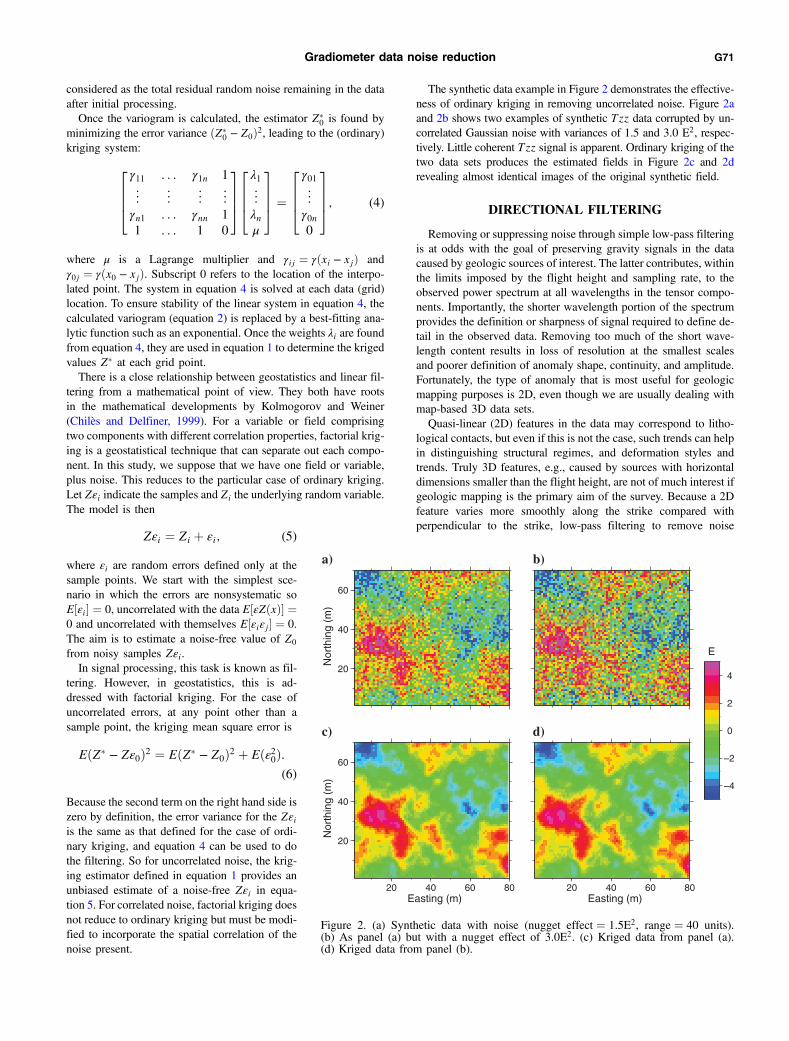
The synthetic data example in Figure 2 demonstrates the effective-ness of ordinary kriging in removing uncorrelated noise. Figure 2aand 2b shows two examples of synthetic Tzz data corrupted by un-correlated Gaussian noise with variances of 1.5 and 3.0 E2, respec-tively. Little coherent Tzz signal is apparent. Ordinary kriging of thetwo data sets produces the estimated fields in Figure 2c and 2drevealing almost identical images of the original synthetic field.

DIRECTIONAL FILTERING

Removing or suppressing noise through simple low-pass filteringis at odds with the goal of preserving gravity signals in the datacaused by geologic sources of interest. The latter contributes, withinthe limits imposed by the flight height and sampling rate, to theobserved power spectrum at all wavelengths in the tensor compo-nents. Importantly, the shorter wavelength portion of the spectrumprovides the definition or sharpness of signal required to define de-tail in the observed data. Removing too much of the short wave-length content results in loss of resolution at the smallest scalesand poorer definition of anomaly shape, continuity, and amplitude.Fortunately, the type of anomaly that is most useful for geologicmapping purposes is 2D, even though we are usually dealing withmap-based 3D data sets.Quasi-linear (2D) features in the data may correspond to litho-

logical contacts, but even if this is not the case, such trends can helpin distinguishing structural regimes, and deformation styles andtrends. Truly 3D features, e.g., caused by sources with horizontaldimensions smaller than the flight height, are not of much interest ifgeologic mapping is the primary aim of the survey. Because a 2Dfeature varies more smoothly along the strike compared withperpendicular to the strike, low-pass filtering to remove noise

20

40

60

Nor

thin

g (m

)

20

40

60

Nor

thin

g (m

)

20 40 60 80Easting (m)

20 40 60 80Easting (m)

a) b)

c) d)

–4

–2

0

2

4

E

Figure 2. (a) Synthetic data with noise (nugget effect ¼ 1.5E2, range ¼ 40 units).(b) As panel (a) but with a nugget effect of 3.0E2. (c) Kriged data from panel (a).(d) Kriged data from panel (b).

Gradiometer data noise reduction G71

can be tuned to take this into account. Short-wavelength featuresalong the strike are preferentially removed while being preservedin the cross-strike direction. In this fashion, short-wavelength com-ponents that provide the detailed definition of the 2D features areunaffected, whereas the short-wavelength noise that overprints anddisrupts along strike trends is suppressed. This is the essence of thecontact lineament processing approach of Brewster (2013). Thiskind of varying directional low-pass filter is used in image process-ing for the detection of object edges from noisy data and the robustdetection of lines in computer vision applications (e.g., Freemanand Adelson, 1991; Geusebroek et al., 2003).In seismic data processing, structure-oriented filtering or smooth-

ing (Fehmers and Hocker, 2003; Hale, 2009) uses similar principleson seismic images to enhance reflection continuity while preservingdiscontinuities such as faults. A simpler form of directional filteringis the basis of microleveling of aeromagnetic data, where short-wavelength variations perpendicular to the flight-line directionare suppressed (Minty, 1991). In this case, only a single filter di-rection is needed for the whole data set. Enhancing the continuityof linear features in aeromagnetic data is also the goal of severaltrend reinforcement algorithms that use approaches that differfrom directional filtering, e.g., Keating (1997) and Smith andO’Connell (2005).The successful application of a directional filter requires the ori-

entation of the filter to be known at each grid point. Several optionsexist to calculate this orientation, for example, by computing a spa-tial average in several directions and then choosing some measure todefine the optimum direction. This could be done using the spatialaverage that is closest to the original grid value or using the maxi-mum spatial average (Lakshmanan, 2004).For gradiometer data applications, we have the advantage of

knowing that the major trends in the data are caused by the dom-inant geologic strike of the causative bodies. The strike can be de-termined from the complete gradient tensor or from each tensorcomponent separately. Two methods exist for finding the strikeof a 2D body from the gradient tensor. The first is based on findinga rotation angle θ such that the sum of squares of the first row of therotated gradient tensor reaches a minimum (Pedersen and Rasmus-sen, 1990). This strike angle value is given by solutions to

tan 2θ ¼ 2½TxyðTxxþ TyyÞ þ TxzTyz�Txx2 − Tyy2 þ Txz2 − Tyz2

: (7)

The second approach is based on first calculating the eigenvaluesand eigenvectors of the gradient tensor matrix. Beiki and Pedersen(2010) note that the eigenvector associated with the smallest eigen-value gives the strike direction of a simple line source. For quasi-2Dbodies, which are thicker and dike-like, the same eigenvector can beused to estimate the strike direction. Both of these approaches as-sume that the tensor components are produced by a 2D or quasi-2Dbody. To verify this assumption, the dimensionality invariant Igiven by Pedersen and Rasmussen (1990) can be used. It variesfrom zero for a 2D body to unity for a 3D source, so using valuesof I < 0.3 is a practical definition of two dimensionality for real data(Beiki and Pedersen, 2010). Similarly, values of I can be plotted forthe whole data set, and a threshold can be chosen.The final method, which is adopted in this work, does not require

the complete gradient tensor values simultaneously and is not relianton assumptions regarding the dimensionality of the source bodies. Itdetermines a strike direction for each tensor component independ-ently, based on the two orthogonal horizontal gradients of the com-ponent at each grid point. Due to noise, using horizontal gradientsdirectly can lead to highly variable strike directions unsuitable forfurther processing. Therefore, to reduce noise effects on strike es-timates, the component data are first low-pass filtered. Second,rather than using calculated horizontal gradients from finitedifferences, the strike direction is found from fitting a plane, ina least-squares sense, to a windowed portion of a given component.A 5 × 5window is used for the planar surface fit. If the fitted planehas the form axþ bxþ c ¼ 0, then the strike direction θ is given bytan−1 ð−c∕bÞ, where θ is measured clockwise from the north. Usinga finite window coupled with some low-pass filtering producesmore continuous strike estimates that are suitable for use in the sub-sequent directional filtering.The estimated strike direction at each grid point defines the ori-

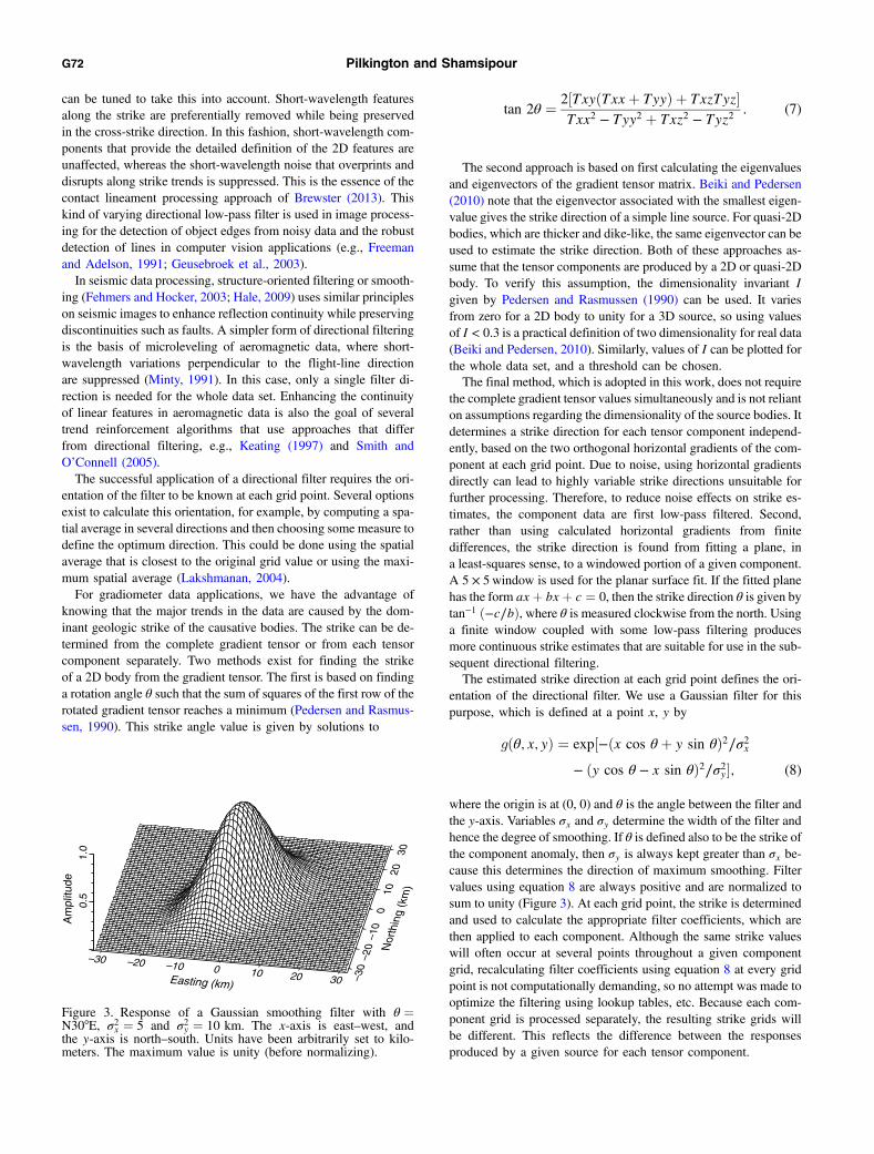
entation of the directional filter. We use a Gaussian filter for thispurpose, which is defined at a point x, y by

gðθ; x; yÞ ¼ exp½−ðx cos θ þ y sin θÞ2∕σ2x− ðy cos θ − x sin θÞ2∕σ2y�; (8)

where the origin is at (0, 0) and θ is the angle between the filter andthe y-axis. Variables σx and σy determine the width of the filter andhence the degree of smoothing. If θ is defined also to be the strike ofthe component anomaly, then σy is always kept greater than σx be-cause this determines the direction of maximum smoothing. Filtervalues using equation 8 are always positive and are normalized tosum to unity (Figure 3). At each grid point, the strike is determinedand used to calculate the appropriate filter coefficients, which arethen applied to each component. Although the same strike valueswill often occur at several points throughout a given componentgrid, recalculating filter coefficients using equation 8 at every gridpoint is not computationally demanding, so no attempt was made tooptimize the filtering using lookup tables, etc. Because each com-ponent grid is processed separately, the resulting strike grids willbe different. This reflects the difference between the responsesproduced by a given source for each tensor component.

–30 –20 –10 0 10 20 30Easting (km)

–30

–20

–10

010

2030

Nor

thin

g (k

m)

0.5

1.0

Am

plitu

de

Figure 3. Response of a Gaussian smoothing filter with θ ¼N30°E, σ2x ¼ 5 and σ2y ¼ 10 km. The x-axis is east–west, andthe y-axis is north–south. Units have been arbitrarily set to kilo-meters. The maximum value is unity (before normalizing).

G72 Pilkington and Shamsipour

ST. GEORGE’S BAY SURVEY

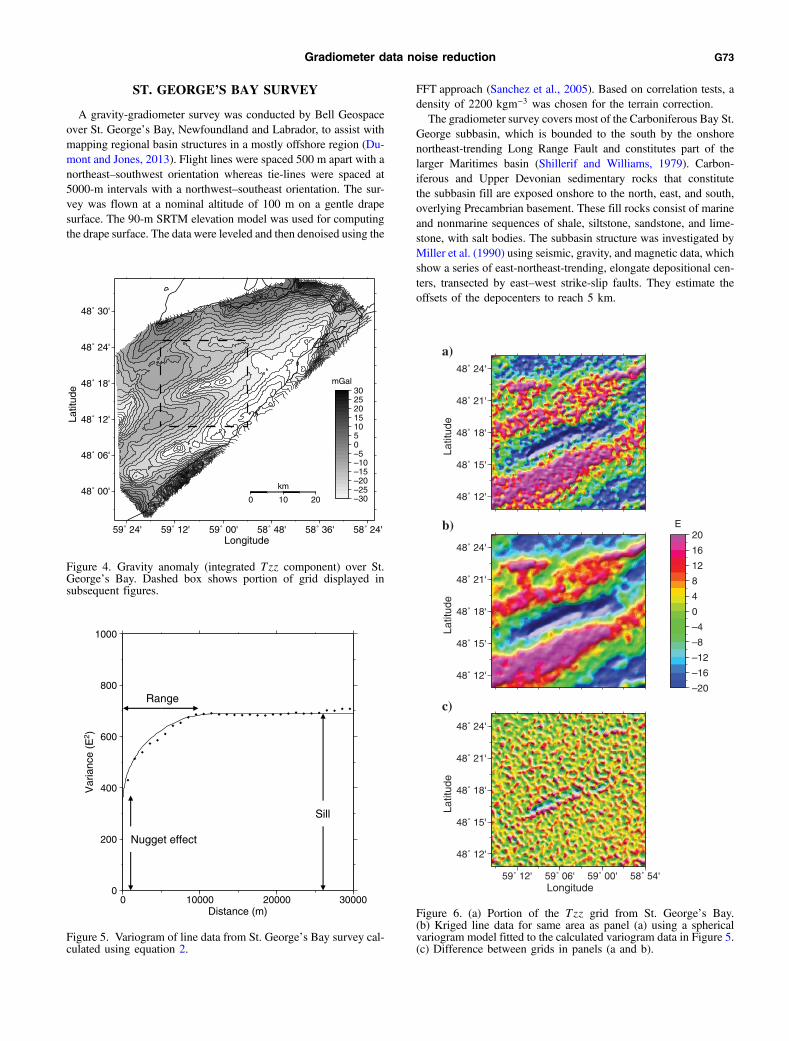
A gravity-gradiometer survey was conducted by Bell Geospaceover St. George’s Bay, Newfoundland and Labrador, to assist withmapping regional basin structures in a mostly offshore region (Du-mont and Jones, 2013). Flight lines were spaced 500 m apart with anortheast–southwest orientation whereas tie-lines were spaced at5000-m intervals with a northwest–southeast orientation. The sur-vey was flown at a nominal altitude of 100 m on a gentle drapesurface. The 90-m SRTM elevation model was used for computingthe drape surface. The data were leveled and then denoised using the

FFT approach (Sanchez et al., 2005). Based on correlation tests, adensity of 2200 kgm−3 was chosen for the terrain correction.The gradiometer survey covers most of the Carboniferous Bay St.

George subbasin, which is bounded to the south by the onshorenortheast-trending Long Range Fault and constitutes part of thelarger Maritimes basin (Shillerif and Williams, 1979). Carbon-iferous and Upper Devonian sedimentary rocks that constitutethe subbasin fill are exposed onshore to the north, east, and south,overlying Precambrian basement. These fill rocks consist of marineand nonmarine sequences of shale, siltstone, sandstone, and lime-stone, with salt bodies. The subbasin structure was investigated byMiller et al. (1990) using seismic, gravity, and magnetic data, whichshow a series of east-northeast-trending, elongate depositional cen-ters, transected by east–west strike-slip faults. They estimate theoffsets of the depocenters to reach 5 km.

59˚ 24' 59˚ 12' 59˚ 00' 58˚ 48' 58˚ 36' 58˚ 24'

48˚ 00'

48˚ 06'

48˚ 12'

48˚ 18'

48˚ 24'

48˚ 30'

0 10 20

km

Longitude

Latit

ude

–30–25–20–15–10–5051015202530

mGal

Figure 4. Gravity anomaly (integrated Tzz component) over St.George’s Bay. Dashed box shows portion of grid displayed insubsequent figures.

0

200

400

600

800

1000

Var

ianc

e (E

2 )

0 10000 20000 30000Distance (m)

Range

Nugget effect

Sill

Figure 5. Variogram of line data from St. George’s Bay survey cal-culated using equation 2.

48˚ 12'

48˚ 15'

48˚ 18'

48˚ 21'

48˚ 24'

48˚ 12'

48˚ 15'

48˚ 18'

48˚ 21'

48˚ 24'

59˚ 12' 59˚ 06' 59˚ 00' 58˚ 54'

48˚ 12'

48˚ 15'

48˚ 18'

48˚ 21'

48˚ 24'

b)

a)

c)

Longitude

Latit

ude

Latit

ude

Latit

ude

–20

–16

–12

–8

–4

0

4

8

12

16

20E

Figure 6. (a) Portion of the Tzz grid from St. George’s Bay.(b) Kriged line data for same area as panel (a) using a sphericalvariogram model fitted to the calculated variogram data in Figure 5.(c) Difference between grids in panels (a and b).

Gradiometer data noise reduction G73

The Bay St. George subbasin forms a half-graben deepening to the southeast, with sedimentthicknesses reaching 6 km. The presence of astrong basement reflector in the seismic dataand its good correlation with the regional gravitytrends indicate that the larger gravity lows arecaused by the thickest sediment accumulationsin the subbasin. Some evaporites that have beendrilled are associated with shorter wavelengthgravity lows. The study of Miller et al. (1990)is based on offshore underwater gravity stationswith 6-km spacing. The new AGG data (250 mgrid spacing, Figure 4) vastly improve the defi-nition of the depocenters, accentuating theirelongated shape and strong northeastern align-ment. The relatively smooth, featureless northernpart of the subbasin shown in the maps of Milleret al. (1990) now exhibits the strong lateral grav-ity gradients similar in amplitude to those foundfurther to the south.

NOISE REDUCTION OFST. GEORGE’S BAY DATA

Kriging

The first step in kriging is calculating the var-iogram of the data using equation 2. This is doneusing the line data for the St. George’s Bay sur-vey, which does not provide an isotropic distri-bution of sample locations. The along-linesample distance is ∼80 m, and the line spacingis 500 m. Having a smaller sample spacing alongflight lines than in the crossline direction has alimited effect on the variogram calculation forseveral reasons. The tie lines at every 5000 mprovide some samples in the crossline direction,but more importantly, the processing of the rawAGG data is grid-based (grid interval 250 m),and the final line data are actually resampledfrom the processed grid. Therefore, informationat wavelengths less than the grid Nyquist wave-length of 500 m is limited. Furthermore, for theSt. George’s Bay data, the calculated variogramin Figure 5 is reliably defined by data separatedby distances greater than 500 m. It shows a range,or maximum correlation distance, of about 10 kmand a nugget effect of ∼370 E2 (standarddeviation 19.2 E). The nugget effect providesan estimate of the noise level in the data andis similar to that for another gradiometer surveyof similar vintage: 16.7 E for the Strange Lakesurvey discussed by Keating and Pilkington(2013). As noted by them, the nugget effect ismuch higher than published measurement noiselevels (6 E), but it reflects a more practical esti-mate by including all other sources of noisepresent. A spherical, isotropic model was fittedto the variogram (Figure 5), and the line datawas gridded at a 250-m interval using ordinary

48˚ 12'

48˚ 15'

48˚ 18'

48˚ 21'

48˚ 24'

59˚ 12' 59˚ 06' 59˚ 00' 58˚ 54'

48˚ 12'

48˚ 15'

48˚ 18'

48˚ 21'

48˚ 24'

59˚ 12' 59˚ 06' 59˚ 00' 58˚ 54'

a) b)

c) d)

LongitudeLongitude

Latit

ude

Latit

ude

–20

–16

–12

–8

–4

0

4

8

12

16

20E

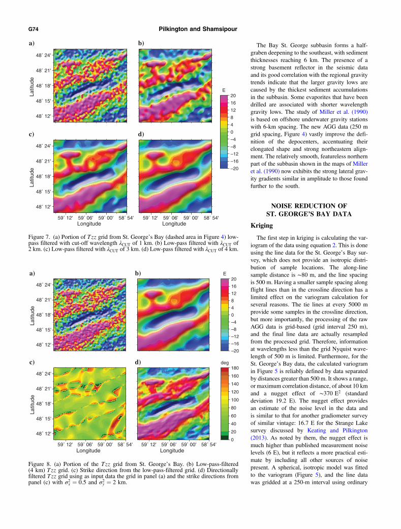
Figure 7. (a) Portion of Tzz grid from St. George’s Bay (dashed area in Figure 4) low-pass filtered with cut-off wavelength λCUT of 1 km. (b) Low-pass filtered with λCUT of2 km. (c) Low-pass filtered with λCUT of 3 km. (d) Low-pass filtered with λCUT of 4 km.

48˚ 12'

48˚ 15'

48˚ 18'

48˚ 21'

48˚ 24'

59˚ 12' 59˚ 06' 59˚ 00' 58˚ 54'

48˚ 12'

48˚ 15'

48˚ 18'

48˚ 21'

48˚ 24'

59˚ 12' 59˚ 06' 59˚ 00' 58˚ 54'

a) b)

c) d)

LongitudeLongitude

Latit

ude

Latit

ude

–20

–16

–12

–8

–4

0

4

8

12

16

20E

0

20

40

60

80

100

120

140

160

180deg

Figure 8. (a) Portion of the Tzz grid from St. George’s Bay. (b) Low-pass-filtered(4 km) Tzz grid. (c) Strike direction from the low-pass-filtered grid. (d) Directionallyfiltered Tzz grid using as input data the grid in panel (a) and the strike directions frompanel (c) with σ2x ¼ 0.5 and σ2y ¼ 2 km.

G74 Pilkington and Shamsipour

kriging (equations 1 and 4). The kriged data in Figure 6 show asignificant reduction in uncorrelated noise level, resulting in the ap-pearance of more coherent gradient features throughout the area.With the suppression of shorter wavelength components, the krigeddata are generally smoother than the gridded (minimum curvature)line data (Figure 6a), leading to some loss in definition of loweramplitude trends. The kriged values are, nonetheless, optimal inthe sense of being estimated from an interpolator (equation 1) basedon the data themselves, and not from an arbitrary interpolator suchas the minimum curvature operator. The difference between stan-dard minimum curvature gridding and kriging is given in Figure 6c,showing the mostly uncorrelated components removed by thekriging.

Directional filtering

Directional filtering involves two steps: determining a strike di-rection and designing and implementing a Gaussian smoothing fil-ter. Calculating the strike direction for each of the input componentgrids requires choosing a cut-off wavelength λLP for the low-passfiltering used. The requirements of this stage of filtering are similarto that of low-pass filtering to remove noise. If λLP is too large, thenreal geologic signal is lost or distorted, but if λLP is too small, thenthe estimated strike directions will be contaminated by noise. Asuitable value for the cut-off wavelength is best found by first vis-ually estimating the longest wavelength in the data that appearsnoisy. Trial and error filtering using values smaller and larger thanthis wavelength can then be carried out to check its validity. Figure 7shows a portion of the St. George’s Bay Tzz component data fil-tered using values of λLP between 1 and 4 km. For λLP ¼ 1 km,noise still dominates the data set. Using an λLP of 2 or 3 km revealsmore underlying geologic signal, with the latter grid reflectingmostly the known east-northeast–west-southwest structural trendscharacteristic of the St. George’s Bay subbasin. Our preferredchoice for this example is the result in Figure 7d, using λLP ¼4 km, which shows that the undulating margins of the main anoma-lies seen in Figure 7b and 7c, most likely due to smoothed residualnoise, are now absent.For the Gaussian filter defined in equation 2, its frequency re-

sponse is easily calculated because the Fourier transform of a Gaus-sian function expð−x2∕σ2Þ is the Gaussian expð−k2σ2∕4Þ, where kis the wavenumber. This gives the relationship, λCUT ¼ πσ, whereλCUT is the wavelength at which the frequency response of the filterfalls to 1∕e of the maximum. From real data tests, using a value ofσx (where σx < σy in equation 8), about half of λLP was found to bea practically reliable choice, balancing the need for detail in the finalimage versus noise amplification. Additionally, a ratio of σy∕σx of∼4 appears to be a useful value. If σy is too small, the directionaleffects of the Gaussian filter diminish, and obviously disappear ifσx ¼ σy. When σy is too large, the filtered image can appear streakyand unrealistic due to too much smoothing along strike. Fortunately,there is some flexibility in the choice of λLP, σx, and σy, such thatsome variation (�25%) in these parameters can be tolerated withonly fairly minor effects on the filtered results.The directional filtering procedure is carried out independently

on each tensor component. As a result, the tensor components mightnot be internally consistent, and not satisfy Laplace’s equation andthe well-known relationships between components that it implies(e.g., Barnes and Lumley, 2011). Consequently, the componentsmust be made consistent through, for example, least-squares esti-

mation of a common gravity potential, from which each componentcan be subsequently recalculated (Sanchez et al., 2005). Anyresidual noise effects in the data that are not Laplacian will be re-moved with this procedure. Conversely, any noise components thatdo satisfy Laplace’s equation will remain unaffected.Figure 8 shows each of the stages of directional filtering dis-

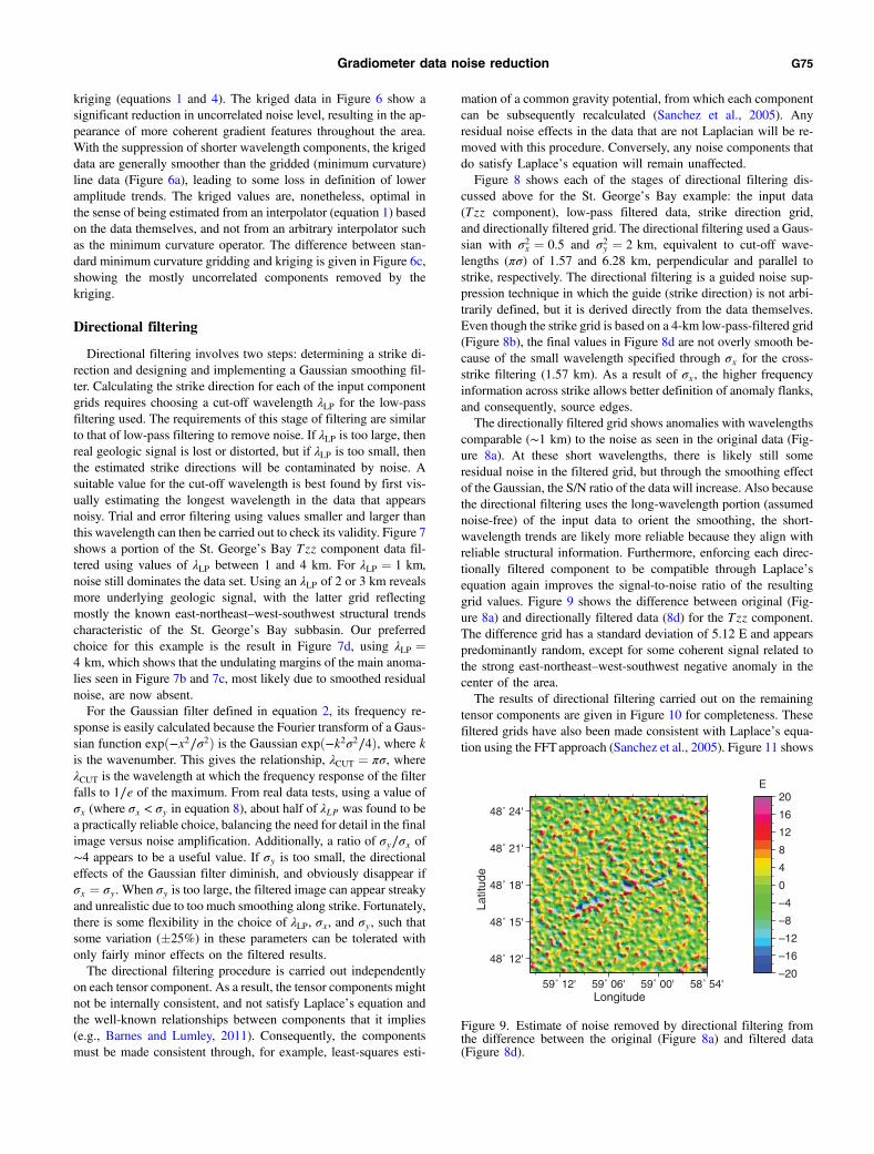
cussed above for the St. George’s Bay example: the input data(Tzz component), low-pass filtered data, strike direction grid,and directionally filtered grid. The directional filtering used a Gaus-sian with σ2x ¼ 0.5 and σ2y ¼ 2 km, equivalent to cut-off wave-lengths (πσ) of 1.57 and 6.28 km, perpendicular and parallel tostrike, respectively. The directional filtering is a guided noise sup-pression technique in which the guide (strike direction) is not arbi-trarily defined, but it is derived directly from the data themselves.Even though the strike grid is based on a 4-km low-pass-filtered grid(Figure 8b), the final values in Figure 8d are not overly smooth be-cause of the small wavelength specified through σx for the cross-strike filtering (1.57 km). As a result of σx, the higher frequencyinformation across strike allows better definition of anomaly flanks,and consequently, source edges.The directionally filtered grid shows anomalies with wavelengths

comparable (∼1 km) to the noise as seen in the original data (Fig-ure 8a). At these short wavelengths, there is likely still someresidual noise in the filtered grid, but through the smoothing effectof the Gaussian, the S/N ratio of the data will increase. Also becausethe directional filtering uses the long-wavelength portion (assumednoise-free) of the input data to orient the smoothing, the short-wavelength trends are likely more reliable because they align withreliable structural information. Furthermore, enforcing each direc-tionally filtered component to be compatible through Laplace’sequation again improves the signal-to-noise ratio of the resultinggrid values. Figure 9 shows the difference between original (Fig-ure 8a) and directionally filtered data (8d) for the Tzz component.The difference grid has a standard deviation of 5.12 E and appearspredominantly random, except for some coherent signal related tothe strong east-northeast–west-southwest negative anomaly in thecenter of the area.The results of directional filtering carried out on the remaining

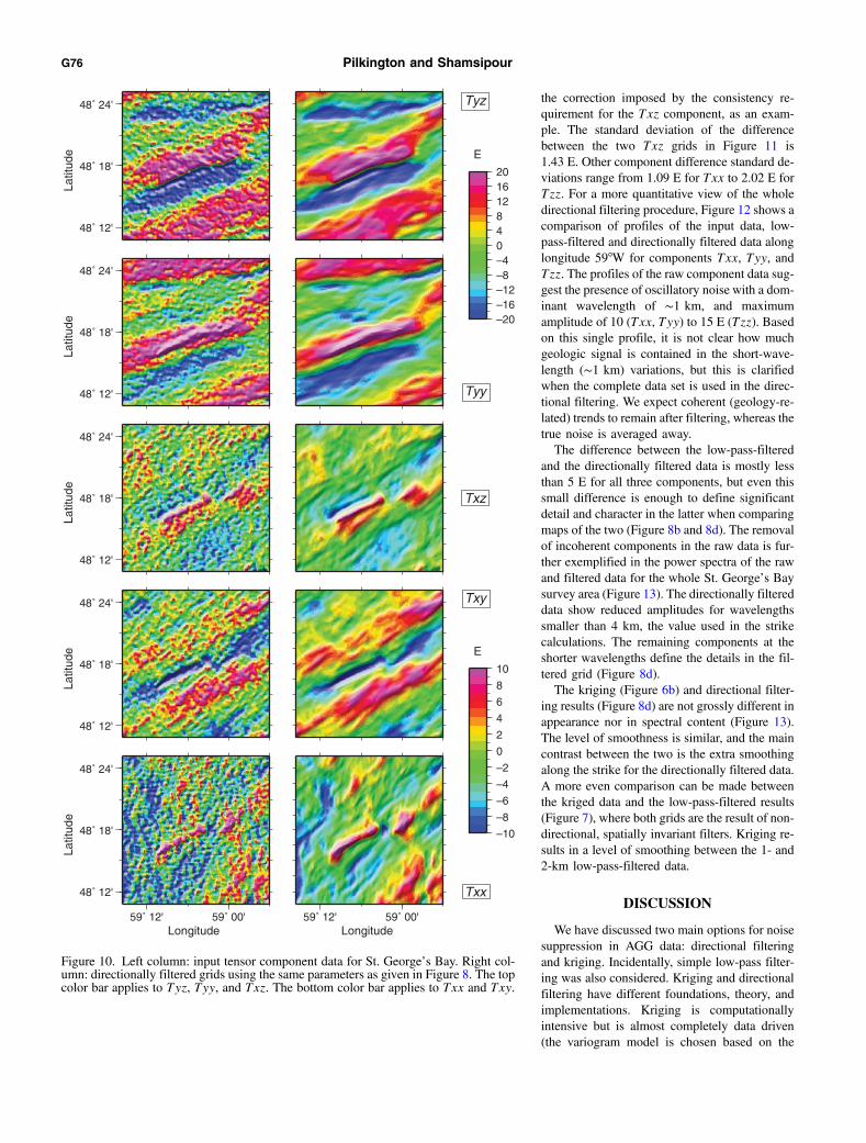
tensor components are given in Figure 10 for completeness. Thesefiltered grids have also been made consistent with Laplace’s equa-tion using the FFTapproach (Sanchez et al., 2005). Figure 11 shows

59˚ 12' 59˚ 06' 59˚ 00' 58˚ 54'

48˚ 12'

48˚ 15'

48˚ 18'

48˚ 21'

48˚ 24'

–20

–16

–12

–8

–4

0

4

8

12

16

20E

Longitude

Latit

ude

Figure 9. Estimate of noise removed by directional filtering fromthe difference between the original (Figure 8a) and filtered data(Figure 8d).

Gradiometer data noise reduction G75

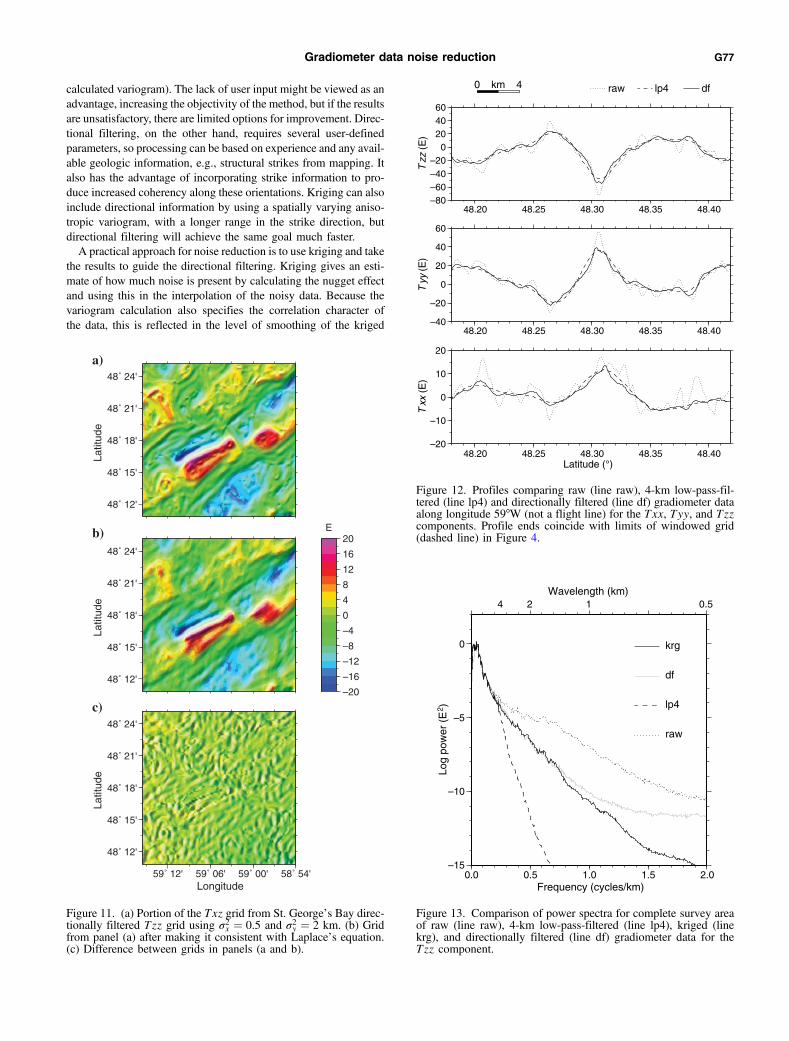
the correction imposed by the consistency re-quirement for the Txz component, as an exam-ple. The standard deviation of the differencebetween the two Txz grids in Figure 11 is1.43 E. Other component difference standard de-viations range from 1.09 E for Txx to 2.02 E forTzz. For a more quantitative view of the wholedirectional filtering procedure, Figure 12 shows acomparison of profiles of the input data, low-pass-filtered and directionally filtered data alonglongitude 59°W for components Txx, Tyy, andTzz. The profiles of the raw component data sug-gest the presence of oscillatory noise with a dom-inant wavelength of ∼1 km, and maximumamplitude of 10 (Txx, Tyy) to 15 E (Tzz). Basedon this single profile, it is not clear how muchgeologic signal is contained in the short-wave-length (∼1 km) variations, but this is clarifiedwhen the complete data set is used in the direc-tional filtering. We expect coherent (geology-re-lated) trends to remain after filtering, whereas thetrue noise is averaged away.The difference between the low-pass-filtered

and the directionally filtered data is mostly lessthan 5 E for all three components, but even thissmall difference is enough to define significantdetail and character in the latter when comparingmaps of the two (Figure 8b and 8d). The removalof incoherent components in the raw data is fur-ther exemplified in the power spectra of the rawand filtered data for the whole St. George’s Baysurvey area (Figure 13). The directionally filtereddata show reduced amplitudes for wavelengthssmaller than 4 km, the value used in the strikecalculations. The remaining components at theshorter wavelengths define the details in the fil-tered grid (Figure 8d).The kriging (Figure 6b) and directional filter-

ing results (Figure 8d) are not grossly different inappearance nor in spectral content (Figure 13).The level of smoothness is similar, and the maincontrast between the two is the extra smoothingalong the strike for the directionally filtered data.A more even comparison can be made betweenthe kriged data and the low-pass-filtered results(Figure 7), where both grids are the result of non-directional, spatially invariant filters. Kriging re-sults in a level of smoothing between the 1- and2-km low-pass-filtered data.

DISCUSSION

We have discussed two main options for noisesuppression in AGG data: directional filteringand kriging. Incidentally, simple low-pass filter-ing was also considered. Kriging and directionalfiltering have different foundations, theory, andimplementations. Kriging is computationallyintensive but is almost completely data driven(the variogram model is chosen based on the

59˚ 12' 59˚ 00'

48˚ 12'

48˚ 18'

48˚ 24'

59˚ 12' 59˚ 00'

48˚ 12'

48˚ 18'

48˚ 24'

48˚ 12'

48˚ 18'

48˚ 24'

48˚ 12'

48˚ 18'

48˚ 24'

48˚ 12'

48˚ 18'

48˚ 24'

Txx

Txy

Txz

Tyy

Tyz

LongitudeLongitude

Latit

ude

Latit

ude

Latit

ude

Latit

ude

Latit

ude

–10

–8

–6

–4

–2

0

2

4

6

8

10

E

–20–16–12–8–4048121620

E

Figure 10. Left column: input tensor component data for St. George’s Bay. Right col-umn: directionally filtered grids using the same parameters as given in Figure 8. The topcolor bar applies to Tyz, Tyy, and Txz. The bottom color bar applies to Txx and Txy.

G76 Pilkington and Shamsipour

calculated variogram). The lack of user input might be viewed as anadvantage, increasing the objectivity of the method, but if the resultsare unsatisfactory, there are limited options for improvement. Direc-tional filtering, on the other hand, requires several user-definedparameters, so processing can be based on experience and any avail-able geologic information, e.g., structural strikes from mapping. Italso has the advantage of incorporating strike information to pro-duce increased coherency along these orientations. Kriging can alsoinclude directional information by using a spatially varying aniso-tropic variogram, with a longer range in the strike direction, butdirectional filtering will achieve the same goal much faster.A practical approach for noise reduction is to use kriging and take

the results to guide the directional filtering. Kriging gives an esti-mate of how much noise is present by calculating the nugget effectand using this in the interpolation of the noisy data. Because thevariogram calculation also specifies the correlation character ofthe data, this is reflected in the level of smoothing of the kriged

48˚ 12'

48˚ 15'

48˚ 18'

48˚ 21'

48˚ 24'

48˚ 12'

48˚ 15'

48˚ 18'

48˚ 21'

48˚ 24'

59˚ 12' 59˚ 06' 59˚ 00' 58˚ 54'

48˚ 12'

48˚ 15'

48˚ 18'

48˚ 21'

48˚ 24'

b)

a)

c)

Longitude

Latit

ude

Latit

ude

Latit

ude

–20

–16

–12

–8

–4

0

4

8

12

16

20E

Figure 11. (a) Portion of the Txz grid from St. George’s Bay direc-tionally filtered Tzz grid using σ2x ¼ 0.5 and σ2y ¼ 2 km. (b) Gridfrom panel (a) after making it consistent with Laplace’s equation.(c) Difference between grids in panels (a and b).

–20

–10

0

10

20

Txx

(E

)

48.20 48.25 48.30 48.35 48.40Latitude (°)

–40

–20

0

20

40

60

Tyy

(E)

48.20 48.25 48.30 48.35 48.40

–80–60–40–20

0204060

Tzz

(E

)

48.20 48.25 48.30 48.35 48.40

raw lp4 df0 km 4

Figure 12. Profiles comparing raw (line raw), 4-km low-pass-fil-tered (line lp4) and directionally filtered (line df) gradiometer dataalong longitude 59°W (not a flight line) for the Txx, Tyy, and Tzzcomponents. Profile ends coincide with limits of windowed grid(dashed line) in Figure 4.

–15

–10

–5

0

Log

pow

er (

E2 )

0.0 0.5 1.0 1.5 2.0Frequency (cycles/km)

4 2 1 0.5

raw

lp4

df

krg

Wavelength (km)

Figure 13. Comparison of power spectra for complete survey areaof raw (line raw), 4-km low-pass-filtered (line lp4), kriged (linekrg), and directionally filtered (line df) gradiometer data for theTzz component.

Gradiometer data noise reduction G77

values. The processing parameters required by directional filteringcan then be tuned to give a similar level of smoothness and noisesuppression to the kriging results, but with the advantage of keepingmore short-wavelength information in the cross-strike direction forbetter trend definition.

CONCLUSION

Ordinary kriging and directional filtering are shown to be viableoptions for noise suppression of gravity-gradiometer data. Krigingis based on the statistical character of the data and produces esti-mates with a commensurate level of smoothness and noise reduc-tion. For directional filtering, the degree of smoothing is userdefined but has the advantage of being sensitive to strike informa-tion derived from the data. For the St. George’s Bay survey, bothapproaches successfully reduce noise levels so that coherent, geo-logically meaningful anomaly patterns are revealed. In this particu-lar case, the directional filtering was carried out independently ofthe kriging, but in retrospect, kriging of the data appears useful inguiding the choice of parameters used for filtering.

ACKNOWLEDGMENTS

We thank J. Brewster of Bell Geospace Inc. for providing helpfulinformation and feedback. X. Li, G. Barnes, M. Dransfield, J. Lyrio,and an anonymous reviewer are thanked for useful reviews. Thiswork was done as part of phase IVof the Natural Resources CanadaTargeted Geoscience Initiative. This is Geological Survey of Can-ada contribution 20130507. We thank W. Miles for reviewing anearlier version of the paper.

REFERENCES

Barnes, G., and J. Lumley, 2011, Processing gravity gradient data: Geophys-ics, 76, no. 2, I33–I47, doi: 10.1190/1.3548548.

Beiki, M., and L. B. Pedersen, 2010, Eigenvector analysis of gravity gradienttensor to locate geologic bodies: Geophysics, 75, no. 6, I37–I49, doi: 10.1190/1.3484098.

Boggs, D. B., and M. H. Dransfield, 2004, Analysis of errors in gravity de-rived from the Falcon airborne gravity gradiometer, in R. J. L. Lane, ed.,Airborne Gravity 2004 — Abstracts from the ASEG-PESA AirborneGravity 2004Workshop: Geoscience Australia, record 2004/18, 135–141.

Brewster, J., 2013, Directional filter for processing full tensor gradiometerdata: Bell Geospace, Inc., U.S. Patent application 13/966722.

Chilès, J.-P., and P. Delfiner, 1999, Geostatistics: Modeling spatial uncer-tainty: Wiley.

DiFrancesco, D., 2013, The coming age of gravity gradiometry: Presented at23rd International Geophysical Conference and Exhibition, ASEG.

Dransfield, M., and A. Christensen, 2013, Performance of airbornegravity gradiometers: The Leading Edge, 32, 908–922, doi: 10.1190/tle32080908.1.

Dumont, R., and A. Jones, 2013, Airborne gravity gradiometer surveyof the St-George’s Bay area, parts of NTS 11-O (North Half) and 12-B, Newfoundland and Labrador: Geological Survey of Canada, Open file7411.

Fehmers, G. C., and C. F. W. Hocker, 2003, Fast structural interpretationwith structure-oriented filtering: Geophysics, 68, 1286–1293, doi: 10.1190/1.1598121.

Freeman, W. T., and E. H. Adelson, 1991, The design and use of steerablefilters: IEEE Transactions on Pattern Analysis and Machine Intelligence,13, 891–906, doi: 10.1109/34.93808.

Geusebroek, J.-M., A. W. M. Smeulders, and J. van de Weijer, 2003, Fastanisotropic Gauss filtering: IEEE Transactions on Image Processing, 12,938–943, doi: 10.1109/TIP.2003.812429.

Hale, D., 2009, Structure-oriented smoothing and semblance: Center forWave Phenomena, Report 635.

Hammond, S., and C. A. Murphy, 2003, Air-FTG™: Bell Geospace’s air-borne gravity gradiometer— A description and case study: Preview, 105,22–24.

Keating, P., 1997, Automated trend reinforcement of aeromagnetic data:Geophysical Prospecting, 45, 521–534, doi: 10.1046/j.1365-2478.1997.3450272.x.

Keating, P., and M. Pilkington, 2013, Analysis and reprocessing of airbornegravity gradiometer data over the Strange Lake rare-earth deposit,Quebec-Labrador: The Leading Edge, 32, 940–947, doi: 10.1190/tle32080940.1.

Lakshmanan, V., 2004, A separable filter for directional smoothing: IEEEGeoscience and Remote Sensing Letters, 1, 192–195, doi: 10.1109/LGRS.2004.828178.

Li, Y., 2001, Processing gravity gradiometer data using an equivalent sourcetechnique: 71st Annual International Meeting, SEG, Expanded Abstracts,1466–1469.

Lyrio, J. C. S., L. Tenorio, and Y. Li, 2004, Efficient automatic denoising ofgravity gradiometry data: Geophysics, 69, 772–782, doi: 10.1190/1.1759463.

Matheron, G. F., 1963, Principles of geostatistics: Economic Geology, 58,1246–1266, doi: 10.2113/gsecongeo.58.8.1246.

Miller, H. G., G. J. Kilfoil, and S. T. Peavy, 1990, An integratedgeophysical interpretation of the Carboniferous Bay St. George Subbasin,Western Newfoundland: Bulletin of Canadian Petroleum Geology, 38,320–331.

Minty, B. R. S., 1991, Simple micro-levelling for aeromagnetic data: Explo-ration Geophysics, 22, 591–592, doi: 10.1071/EG991591.

Pedersen, L. B., and T. M. Rasmussen, 1990, The gradient tensor ofpotential field anomalies: Some implications on data collection anddata processing of maps: Geophysics, 55, 1558–1566, doi: 10.1190/1.1442807.

Sanchez, V., D. Sinex, Y. Li, M. Nabighian, D. Wright, and D. Smith, 2005,Processing and inversion of magnetic gradient tensor data for UXO ap-plications: 18th EEGS Symposium on the Applications of Geophysics toEngineering and Environmental Problems, Extended Abstracts, 1193–1202.

Schillerif, S., and H.Williams, 1979, Geology of the Stephenville Map Area,Newfoundland: in Current research, Part A, Geological Survey of Canada,Paper 79-1A, 327-332.

Smith, R. S., and M. D. O’Connell, 2005, Interpolation and gridding ofaliased geophysical data using constrained anisotropic diffusion to en-hance trends: Geophysics, 70, no. 5, V121–V127, doi: 10.1190/1.2080759.

Yuan, Y., D. Huang, Q. Yu, and M. Geng, 2013, Noise filtering of full-grav-ity gradient tensor data: Applied Geophysics, 10, 241–250, doi: 10.1007/s11770-013-0391-3.

G78 Pilkington and Shamsipour