NOISE PERCEPTION, PSYCHOACOUSTIC INDICATORS, AND

Gestão da velocidade e do ruído rodoviário, Guimarães, 2012. ISBN 978-972-8692-70-4 Management of speed and traffic noise, Guimarães, 2012. ISBN 978-972-8692-70-4 166

NOISE PERCEPTION, PSYCHOACOUSTIC INDICATORS, AND TR AFFIC NOISE

Catarina Mendonça

Centro Algoritmi, Universidade do Minho, Centro de Computação Gráfica, Guimarães

E-mail: [email protected]

ABSTRACT

We present an overview of sound characteristics, noise and noise perception. Several sound measures, weightings and psychoacoustic parameters are discussed and compared. Finally, we present some data comparing several psychoacoustic measures and their predictability of traffic noise annoyance and vehicle detection. We propose loudness measures according to Zwicker as a standard for environmental noise assessment, in detriment of the widely accepted A-weighted Leq.

Keywords: Psychoacoustics, Loudness, Sharpness, Roughness, LAeq, Leq, Annoyance INTRODUCTION

Noise and Sound

Noise is among the most prominent forms of pollution in the industrialised and developing regions. This form of pollution can affect people in several physical, psychological and social dimensions, namely by causing auditory lesions, stress, annoyance, distraction, tiredness, or simply by impairing social communication (e.g. Gorai and Pal, 2006; Passchier-Vermeer and Passchier, 2000; Sanz et al, 1993; Freitas et al., 2012).

Physically, noise is a complex stimulus made of several mechanical vibrations or pressure fluctuations that are disseminated in elastic means. Perceptually, when these vibrations reach the human ear, and if they are within the audible frequencies, they will cause nerve excitation and thus produce the mental representation of sound. The auditory representation of a sound depends on specific physical parameters, namely frequency, period, and amplitude.

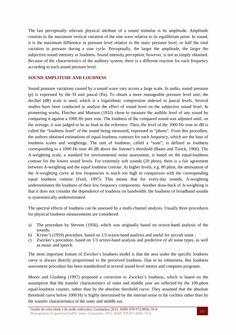
The frequency of a periodic phenomenon, such as a sound wave, is the number of times that the phenomenon repeats itself in a time interval. In acoustics, it is often defined as the number of times the pressure varies around the atmospheric pressure in one second, and it is expressed in Hertz (Hz). Period is defined as the total amount of time it takes for one sound wave to complete a full cycle. The frequency span for auditory sound processing in normal listeners is between 20 and 20.000 Hz. Lower frequency sounds lead to low pitch sensations and high frequency sounds lead to high pitch sensations. The frequency of a sound is relevant for environmental noise assessments, as higher pitch sounds are considered more annoying and more disruptive than lower pitch sounds. In natural environments, however, pure tone sounds (with only one sine wave) are never found. Instead, several sound waves interact and reach the ear simultaneously, influencing the perceived timbre or sound quality. Environmental sounds can therefore be analysed by decomposing them into separate waves or simple harmonics, namely through Fourier analyses.


The last perceptually relevant physical attribute of a sound stimulus is its amplitude. Amplitude consists in the maximum vertical variation of the sine wave relative to its equilibrium point. In sound, it is the maximum difference in pressure level relative to the static pressure level, or half the total variation in pressure during a sine cycle. Perceptually, the larger the amplitude, the larger the subjective sound intensity or loudness. Sound intensity perception, however, is not as simply obtained. Because of the characteristics of the auditory system, there is a different reaction for each frequency according to each sound pressure level.

SOUND AMPLITUDE AND LOUDNESS

Sound pressure variations caused by a sound wave vary across a large scale. In audio, sound pressure (p) is expressed by the SI unit pascal (Pa). To obtain a more manageable pressure level unit, the decibel (dB) scale is used, which is a logarithmic compression indexed to pascal levels. Several studies have been conducted to analyse the effect of sound level on the subjective sound level. In pioneering works, Fletcher and Munson (1933) chose to measure the audible level of any sound by comparing it against a 1000 Hz pure tone. The loudness of the compared sound was adjusted until, on the average, it was judged to be as loud as the reference. Then, the level of the 1000 Hz tone in dB is called the “loudness level” of the sound being measured, expressed in “phons”. From this procedure, the authors obtained estimations of equal-loudness contours for each frequency, which are the base of loudness scales and weightings. The unit of loudness, called a “sone”, is defined as loudness corresponding to a 1000 Hz tone 40 dB above the listener’s threshold (Bauer and Torick, 1966). The A-weighting scale, a standard for environmental noise assessment, is based on the equal-loudness contour for the lowest sound levels. For extremely soft sounds (20 phon), there is a fair agreement between A-weighting and the equal loudness contour. At higher levels, e.g. 80 phon, the attenuation of the A-weighting curve at low frequencies is much too high in comparison with the corresponding equal loudness contour (Festl, 1997). This means that for every-day sounds, A-weighting underestimates the loudness of their low frequency components. Another draw-back of A-weighting is that it does not consider the dependence of loudness on bandwidth: the loudness of broadband sounds is systematically underestimated.

The spectral effects of loudness can be assessed by a multi-channel analysis. Usually three procedures for physical loudness measurements are considered:

a) The procedure by Stevens (1956), which was originally based on octave-band analysis of the sounds;

b) Kryter’s (1959) procedure, based on 1/3 octave-band analysis and useful for aircraft noise ; c) Zwicker’s procedure, based on 1/3 octave-band analysis and predictive of all noise types, as well

as music and speech.

The most important feature of Zwicker’s loudness model is that the area under the specific loudness curve is always directly proportional to the perceived loudness. Due to its robustness, this loudness assessment procedure has been standardized in several sound level meters and computer programs.

Moore and Glasberg (1997) proposed a correction to Zwicker’s loudness, which is based on the assumption that the transfer characteristics of outer and middle year are reflected by the 100-phon equal-loudness counter, rather than by the absolute threshold curve. They assumed that the absolute threshold curve below 1000 Hz is highly determined by the internal noise in the cochlea rather than by the transfer characteristics of the outer and middle ear.


Despite such deterministic approaches to loudness assessment, one final remark should be stressed about its subjective nature. The final perceived sound intensity, or “sensory loudness”, is a complex product also integrating emotional factors and psychological conditioning (Bauer and Torick, 1966). For instance, a person shouting seems louder than a person talking, even when both sounds are equalized in wave amplitude. Next, we will approach other measures that intended to better capture the sound quality or pleasantness.

OTHER PSYCHOACOUSTIC MEASURES

Two other common psychoacoustic measures are sharpness and roughness. Sharpness is a psychoacoustic measure sometimes used in assessing sound quality. Sharpness is a hearing sensation related to frequency. It relates to the sensation of a sharp, high-frequency sound and is the comparison of the amount of high frequency energy to the total energy. This algorithm normalizes the specific loudness spectrum by the total loudness and weights the spectrum according to frequency. The algorithm returns the frequency-weighted result as the specific sharpness versus critical band rate and then integrates the specific sharpness to measure the sharpness. Higher frequency components in the signal generally result in higher sharpness measurements. Roughness is related to sensory dissonance (Parncutt, 1989). It is the beating sensation produced by the interaction of two or more components that are sensed within a certain distance in the inner ear. This distance is referred to as “critical bandwidth” and varies with frequency. According to Parncutt, to calculate the degree of roughness between two pitches, we must first calculate the critical bandwidth for the area around the mean frequency. We then define the roughness as the sum of the roughness of each pair of components.

Recently, Fastl and Zwicker (2007) suggested another psychoacoustic approach: Sensory pleasantness. This approach to sound quality was proposed as a more complex sensation that is influenced by elementary auditory sensations such as roughness, sharpness, tonality, and loudness. They presented a model of weighted estimations of each factor, but such approach still lacks sustained empirical support.

ENVIRONMENTAL NOISE AND VEHICLE DETECTION

Environmental noise assessment is often conducted with a sound level meter. As noise needs to be integrated in time, its measures are often expressed in Leq.

Leq is best described as the average sound level over the period of measurement. It is usually measured A-weighted and hence expressed in LAeq. As the Leq (defined as the Equivalent Continuous Sound Level) is an average, it is settled to a steady value, making it easier to read accurately than with a simple instantaneous Sound Level. Being an average, it also shows the total energy of the noise, so it is a better indicator of potential hearing damage or the likelihood that the noise will generate complaints. The Leq is the main parameter for most serious applications. It is essential for most noise at work assessments and is also the main parameters used for environmental assessments.

In the next section we present some results from traffic noise recordings, noise values, psychoacoustic analyses and their relation to traffic sound annoyance and vehicle detection.


METHODS

Participants

Eighty-nine participants were recruited from educational and social institutions (7-86 years old, average 36.68, SD 22.12). Split into age groups, 26 participants were juvenile (19 years and below, average 12.93, SD 2.31), 27 were early adults (20-39 years, average 27.98, SD 5.33), 19 were middle adults (40-59, average 50.51, SD 5.94) and 17 late adults (60 years and above, average 71.35, SD 6.96). To exclude prior major hearing deficiency all participants underwent audiometric screening tests (250, 1000 and 4000 Hz).

Stimuli and equipment

To record the tyre-noise samples, the selected pavement surfaces for this study were: cobble stones, dense asphalt, and open graded asphalt rubber. The vehicles were a small passenger car (Wolkswagen Polo), a hybrid (Toyota Prius), and a pickup truck (Mitsubishi Strakar). Both the representative sections of the road surfaces and the recording techniques were selected according to the European ISO Standard 11819-1:1997. The controlled pass-by method (CPB) was used, with each single vehicle tyre-road noise recorded with speeds of 30, 40 and, 50 Km/h.

The tyre-road noise was binaurally recorded with a Brüel & Kjaer Head and Torso Simulator (HATS) type 4128-C, a Brüel & Kjaer Pulse Analyzer type 3560-C and the Pulse CPB Analysis software. The noise samples were recorded with the HATS at 7.5 meters from the road centre and at a height of 1.7 meters (for methodological details see Freitas et al., 2012).

From each single vehicle recording, sound samples with a duration of 2 seconds were produced. For all sound samples the final Time-to-Passage (TTP) of the approaching vehicle was fixed to 3.5 seconds; i.e. at the end of the stimulus presentation the vehicle would need 3.5 seconds to cross the line of sight of the observer. To mask the signal (tyre-road sound) five levels of white noise were generated with WaveLab 6: -40, -35, -30, -25 and -20 dBv, corresponding to the LAeq (dBA) values, as listened by the participants, of 62, 67, 72, 77 and 82, respectively. A total of 135 stimuli with signal plus noise were generated with audio software (Ardour): 3 pavements x 3 vehicles x 3 speeds x 5 noise levels.

The stimuli were listened through a computer with a sound card Intel 82801BA-ICH2, a custom built C++ application, and AKG K 271 MKII closed headphones. This system was calibrated to achieve sound pressure levels identical to those recorded in the real scenarios. The values of Loudness were assessed with the Psysound3 application (Cabrera, Ferguson, Rizwi and Schubert, 2008).

PROCEDURE

Annoyance experiment

The annoyance assessment of each participant was performed in a quiet room. All 30 stimuli were also presented channel reversed to avoid interaural biases. The resulting 60 samples were repeated twice (trials). Thus each participant listened to a total of 120 noise trials (30 stimuli x 2 channel sequences x 2 trials). Trials were presented in a pseudo-random order (method of the constant stimulus) to reduce anticipation and expectation interferences. Participants were requested to assess the annoyance of each


noise trial with a 10-graded interval scale from 1 (less annoying) to 10 (very annoying). The interval between trials was variable and depended on the promptness of the participant: after the answer to a given trial (by pressing a number on a keyboard) the next noise sample was presented. Each session, with the 120 trials, lasted for about 14 minutes per participant.

Vehicle detection experiment

Within each trial the participant was presented with two consecutive sound samples, with a fixed gap of 1 second, one with the signal (approaching vehicle ) plus noise and the other with only noise. Both noise backgrounds of each trial had the same level of white noise. The 135 trials were presented in a pseudo-random order (method of constant stimulus). Participants were requested to detect in which of the intervals, i.e., first or second sample, was the approaching vehicle (two-interval forced choice, 2IFC). To avoid biased answers from participants the left-right orientation of the approaching vehicle and the order of intervals were randomized across the 135 trials.

RESULTS

Annoyance and acoustic indicators

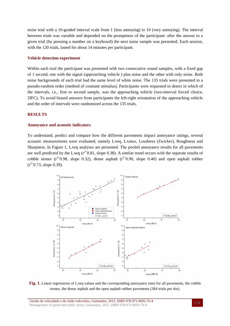
To understand, predict and compare how the different pavements impact annoyance ratings, several acoustic measurements were evaluated, namely LAeq, LAmax, Loudness (Zwicker), Roughness and Sharpness. In Figure 1, LAeq analyses are presented. The pooled annoyance results for all pavements are well predicted by the LAeq (r2=0.81, slope 0.38). A similar trend occurs with the separate results of cobble stones (r2=0.98, slope 0.32), dense asphalt (r2=0.90, slope 0.40) and open asphalt rubber (r2=0.73, slope 0.39).

Fig. 1. Linear regressions of LAeq values and the corresponding annoyance rates for all pavements, the cobble

stones, the dense asphalt and the open asphalt rubber pavements (384 trials per dot).


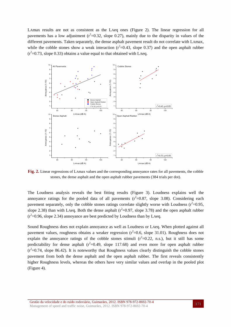
LAmax results are not as consistent as the LAeq ones (Figure 2). The linear regression for all pavements has a low adjustment (r2=0.32, slope 0.27), mainly due to the disparity in values of the different pavements. Taken separately, the dense asphalt pavement result do not correlate with LAmax, while the cobble stones show a weak interaction (r2=0.43, slope 0.37) and the open asphalt rubber (r2=0.73, slope 0.33) obtains a value equal to that obtained with LAeq.

Fig. 2. Linear regressions of LAmax values and the corresponding annoyance rates for all pavements, the cobble

stones, the dense asphalt and the open asphalt rubber pavements (384 trials per dot).

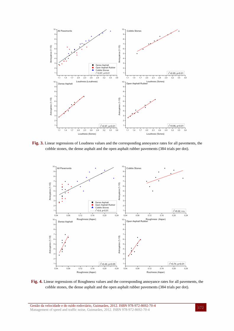
The Loudness analysis reveals the best fitting results (Figure 3). Loudness explains well the annoyance ratings for the pooled data of all pavements (r2=0.87, slope 3.08). Considering each pavement separately, only the cobble stones ratings correlate slightly worse with Loudness (r2=0.95, slope 2.38) than with LAeq. Both the dense asphalt (r2=0.97, slope 3.78) and the open asphalt rubber (r2=0.96, slope 2.34) annoyance are best predicted by Loudness than by LAeq.

Sound Roughness does not explain annoyance as well as Loudness or LAeq. When plotted against all pavement values, roughness obtains a weaker regression (r2=0.6, slope 31.01). Roughness does not explain the annoyance ratings of the cobble stones stimuli (r2=0.22, n.s.), but it still has some predictability for dense asphalt (r2=0.49, slope 117.68) and even more for open asphalt rubber (r2=0.74, slope 86.42). It is noteworthy that Roughness values clearly distinguish the cobble stones pavement from both the dense asphalt and the open asphalt rubber. The first reveals consistently higher Roughness levels, whereas the others have very similar values and overlap in the pooled plot (Figure 4).


Fig. 3. Linear regressions of Loudness values and the corresponding annoyance rates for all pavements, the

cobble stones, the dense asphalt and the open asphalt rubber pavements (384 trials per dot).

Fig. 4. Linear regressions of Roughness values and the corresponding annoyance rates for all pavements, the

cobble stones, the dense asphalt and the open asphalt rubber pavements (384 trials per dot).


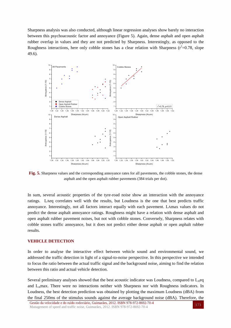
Sharpness analysis was also conducted, although linear regression analyses show barely no interaction between this psychoacoustic factor and annoyance (Figure 5). Again, dense asphalt and open asphalt rubber overlap in values and they are not predicted by Sharpness. Interestingly, as opposed to the Roughness interactions, here only cobble stones has a clear relation with Sharpness (r2=0.78, slope 49.6).

Fig. 5. Sharpness values and the corresponding annoyance rates for all pavements, the cobble stones, the dense

asphalt and the open asphalt rubber pavements (384 trials per dot).

In sum, several acoustic properties of the tyre-road noise show an interaction with the annoyance ratings. LAeq correlates well with the results, but Loudness is the one that best predicts traffic annoyance. Interestingly, not all factors interact equally with each pavement. LAmax values do not predict the dense asphalt annoyance ratings. Roughness might have a relation with dense asphalt and open asphalt rubber pavement noises, but not with cobble stones. Conversely, Sharpness relates with cobble stones traffic annoyance, but it does not predict either dense asphalt or open asphalt rubber results.

VEHICLE DETECTION

In order to analyse the interactive effect between vehicle sound and environmental sound, we addressed the traffic detection in light of a signal-to-noise perspective. In this perspective we intended to focus the ratio between the actual traffic signal and the background noise, aiming to find the relation between this ratio and actual vehicle detection.

Several preliminary analyses showed that the best acoustic indicator was Loudness, compared to LAeq and LAmax. There were no interactions neither with Sharpness nor with Roughness indicators. In Loudness, the best detection prediction was obtained by plotting the maximum Loudness (dBA) from the final 250ms of the stimulus sounds against the average background noise (dBA). Therefore, the


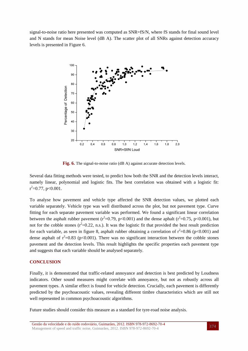
signal-to-noise ratio here presented was computed as SNR=fS/N, where fS stands for final sound level and N stands for mean Noise level (dB A). The scatter plot of all SNRs against detection accuracy levels is presented in Figure 6.

Fig. 6. The signal-to-noise ratio (dB A) against accurate detection levels.

Several data fitting methods were tested, to predict how both the SNR and the detection levels interact, namely linear, polynomial and logistic fits. The best correlation was obtained with a logistic fit: r2=0.77, p<0.001.

To analyse how pavement and vehicle type affected the SNR detection values, we plotted each variable separately. Vehicle type was well distributed across the plot, but not pavement type. Curve fitting for each separate pavement variable was performed. We found a significant linear correlation between the asphalt rubber pavement (r2=0.79, p<0.001) and the dense aphalt (r2=0.75, p<0.001), but not for the cobble stones (r2=0.22, n.s.). It was the logistic fit that provided the best result prediction for each variable, as seen in figure 8, asphalt rubber obtaining a correlation of r2=0.86 (p<0.001) and dense asphalt of r2=0.83 (p<0.001). There was no significant interaction between the cobble stones pavement and the detection levels. This result highlights the specific properties each pavement type and suggests that each variable should be analysed separately.

CONCLUSION

Finally, it is demonstrated that traffic-related annoyance and detection is best predicted by Loudness indicators. Other sound measures might correlate with annoyance, but not as robustly across all pavement types. A similar effect is found for vehicle detection. Crucially, each pavement is differently predicted by the psychoacoustic values, revealing different timbre characteristics which are still not well represented in common psychoacoustic algorithms.

Future studies should consider this measure as a standard for tyre-road noise analysis.


REFERENCES

Bauer, B.B., Torick, E.L. (1966). Researches in loudness measurement. IEEE Transactions on Audio

and Electroacoustics, AU-14(3), pp. 141-151. Fastl, H. (1997). The psychoacoustics of sound-quality evaluation. Acustica united with Acta Acustica,

83, pp. 754-764. Fastl, H., Zwicker, E. (2007). Sharpness and sensory pleasantness. In Psychoacoustic Facts and

Models, Springer-Berlin Heidelberg, pp. 239-246. Fletcher, H., Munson, W.A. (1933). Loudness, its definition, measurement and calculation. Journal of

the Acoustical Society of America, 5, pp. 82.108. Freitas, E., Mendonça, C., Santos, J.A., Murteira, C., Ferreira, J.P., 2012. Traffic noise abatement:

How different pavements, vehicle speeds and traffic densities affect annoyance levels. Transportation Research Part D. 17, 321-326.

Gorai, A.K., Pal, A.K., 2006. Noise and its effect on human being - a review. Journal of Environmental Science and Engineering 48(4), 253-260.

Kryter, K. D. (1959). Scaling human reactions to the sound from an aircraft. Journal of the Acoustical Society of America, 31(11), pp. 1415-1429.

Moore, B.C.J., Glasberg, B.R., Baer, T. (1997). A model for the prediction of thresholds, loudness, and partial loudness. Journal of the Audio Engineering Society, 45(4), pp. 224-240.

Parncutt, R. (1989). Harmony: A psychoacoustical approach. Springer-Verlag: Berlin. Passchier-Vermeer, W., Passchier, W.F., 2000. Noise exposure and public health. Environmental

Health Perspectives 108(1), 123-131. Sanz, S.A., Gracía, A.M., & García, A., 1993. Road traffic noise around schools: a risk for pupils

performance? International Archives of Occupational and Environmental Health 65, 205-207. Stevens, S. S. (1956). Calculation of the loudness of a complex noise. Journal of the Acoustical

Society of America, 28, pp. 807-832. Zwicker, E. (1977). Procedure for calculating loudness of temporally variable sounds. Journal of the

Acoustical Society of America, 62(3), pp.675-682.

Documents

NOISE PERCEPTION, PSYCHOACOUSTIC INDICATORS, AND