NOAA Technical Memorandum GLERL-152

The Impacts of ENSO and AO/NAO on the Interannual Variability of Great Lakes Ice Cover

Xuezhi Bai, Jia Wang, Cynthia Sellinger, Anne Clites, and Raymond AsselNOAA, Great Lakes Environmental Research Laboratory, Ann Arbor, MI

November 2010

UNITED STATESDEPARTMENT OF COMMERCE

Gary LockeSecretary

NATIONAL OCEANIC ANDATMOSPHERIC ADMINISTRATION

Jane LubchencoUnder Secretary for Oceans & AtmosphereNOAA Administrator

2

NOTICE

Mention of a commercial company or product does not constitute an endorsement by the NOAA. Use of information from this publication concerning proprietary products or the tests of such products for publicity or advertising purposes is not authorized. This is GLERL Contribution No. 1561.

This publication is available as a PDF file and can be downloaded from GLERL’s web site: www.glerl.noaa.gov. Hard copies can be requested from GLERLInformation Services, 4840 S. State Rd., Ann Arbor, MI 48108.pubs.glerl@noaa.gov.

NOAA’s Mission – To understand and predict changes in Earth’s environment and conserve and manage coastal and marine resources to meet our nation’s economic, social, and environmental needs.

NOAA’s Mission Goals:

• Protect, restore and manage the use of coastal and ocean resources through an ecosystem approach to management.

• Understand climate variability and change to enhance society’s ability to plan and respond.

• Serve society’s needs for weather and water information.• Support the Nation’s commerce with information for safe, efficient, and envi-

ronmentally sound transportation.• Provide critical support for NOAA’s Mission.

3

TABLE OF CONTENTS

ABSTRACT ............................................................................................................................................... 7

1. INTRODUCTION ................................................................................................................. 7

2. DATA AND METHODS ...................................................................................................... 10 2.1 Winter maximum ice cover ............................................................................................ 10 2.2 NCEP/NCAR reanalysis ................................................................................................ 12 2.3 Climate indices ............................................................................................................... 12 2.4 Methods.......................................................................................................................... 12

3. CLIMATOLOGY, COMPOSITE ATMOSPHERIC CONDITIONS FOR SEVERE AND LEAST ICE COVER ................................................................................................. 13

4. GREAT LAKES ICE COVER AND ENSO ......................................................................... 19

5. GREAT LAKES ICE COVER AND AO .............................................................................. 26

6. INTERFERENCE OF EFFECTS OF ENSO AND AO ON GREAT LAKES ICE COVER......................................................................................................................... 27

7. REGRESSION MODELS FOR GREAT LAKES ICE ........................................................ 37

8. SUMMARY AND CONCLUSIONS .................................................................................... 39

9. ACKNOWLEDGEMENTS ................................................................................................. 41

10. REFERENCES .................................................................................................................... 41

LIST OF FIGURES

Figure 1 (a) 1963-2008 Great Lakes winter maximum ice coverage. (b) Time series of winter AO and ENSO indices from 1963 to 2008. The zero-lag correlations are also calculated: r(AO, ice)=-0.28, r(Nino3.4, ice)=-0.18, r(Nino3.42, ice)=-0.45..............................11

Figure 2 Winter climatology of (a) 700 hPa height, (b) SLP and winds, (c) and SAT in North America. The intervals of 700hPa height, SLP, and SAT are 40 m, 2 hPa, and 3°C, respectively .......................................................................................................14 Figure 3. Composite maps of mean winter 700 hPa height anomalies (relative to the long-term mean in Figure 2a) for those years from 1963 to 2008 when winter ice cover on the Great Lakes was (a) severe, (b) least, and (c) differences between these two cases. Shaded areas indicate differences that are locally significant at the 10% (lighter shaded) and 5% (darker shaded) level based on a two-tailed t test. The intervals are 10 m ....................16

4

Figure 4. Composite maps of mean winter sea level pressure and surface winds anomalies (relative to the long-term mean) for those years from 1963 to 2008 when winter ice cover on the Great Lakes was (a) severe and (b) least. The SLP interval is 0.5 hPa .....................................................................................................................................17

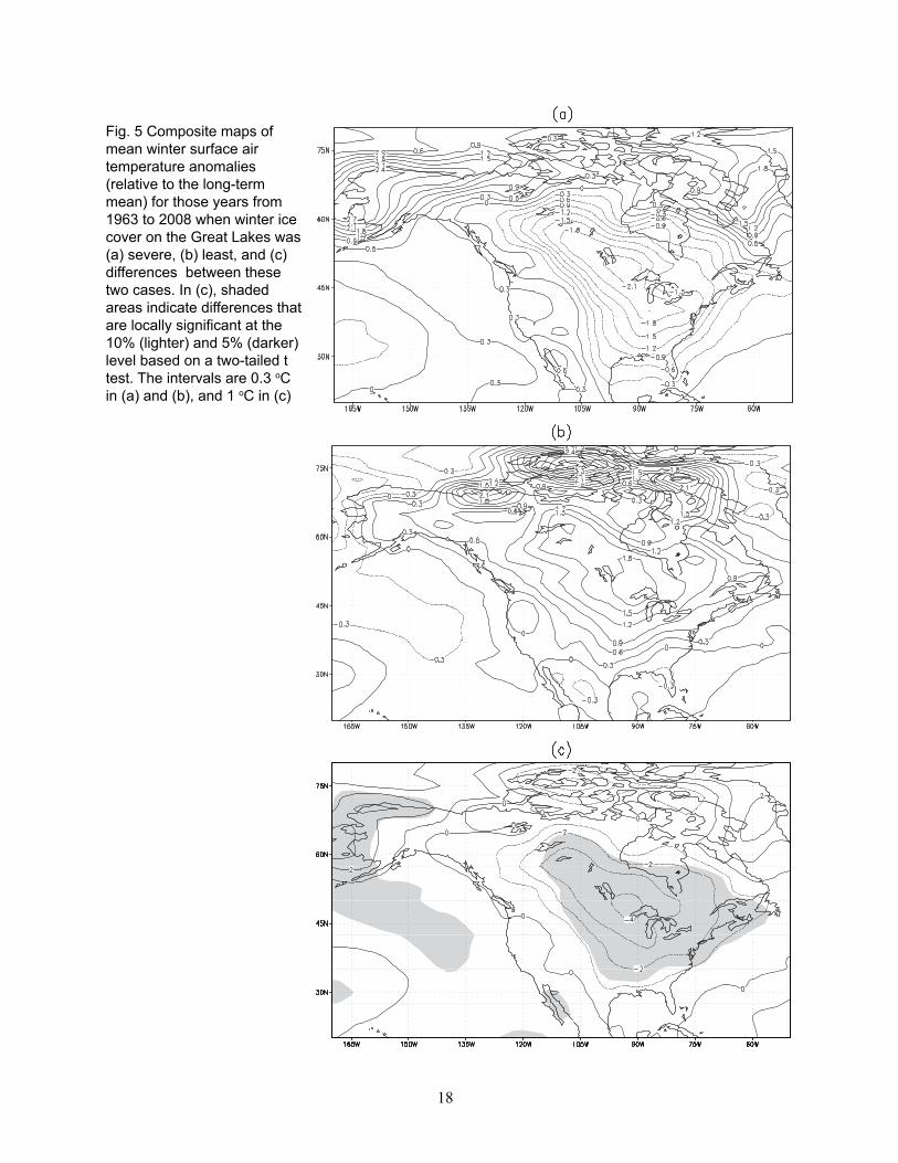
Figure 5. Composite maps of mean winter surface air temperature anomalies (relative to the long-term mean) for those years from 1963 to 2008 when winter ice cover on the Great Lakes was (a) severe, (b) least, and (c) differences between these two cases. In (c), shaded areas indicate differences that are locally significant at the 10% (lighter) and 5% (darker) level based on a two-tailed t test. The intervals are 0.3°C in (a) and (b), and 1°C in (c) .......................................................................................18

Figure 6. The plane scatter plot between ice coverage and ENSO index for the period 1963-2008 ...................................................................................................................................19

Figure 7. Average winter maximum ice coverage for (a) ENSO, (b) AO, and (c) four climate states ............................................................................................................................................21

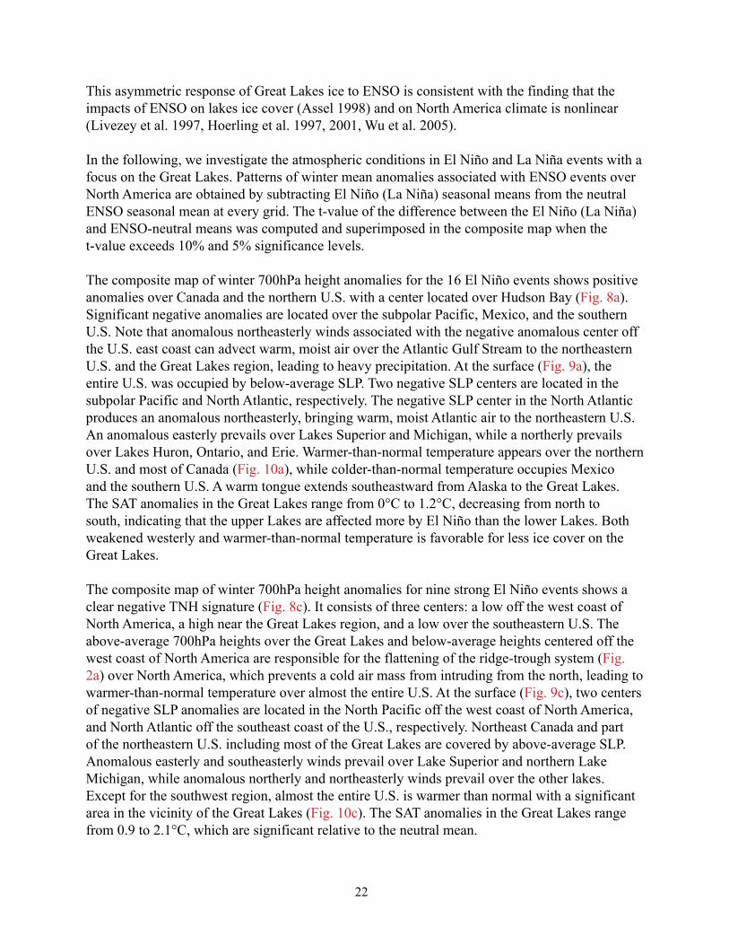
Figure 8. Composite maps of mean winter 700 hPa height temperature anomalies for winters of (a) El Niño, (b) La Niña, (c) strong El Niño, and (d) strong La Niña. Shaded area indicate differences that are locally significant at the 10% (lighter) and 5% (darker) levels based on a two-tailed t-test. The intervals are 10 m. The arrows emphasize the anomalous circulation patterns that advect anomalous warm, moist air from the North Atlantic and the Gulf of Mexico, respectively ...................................................23

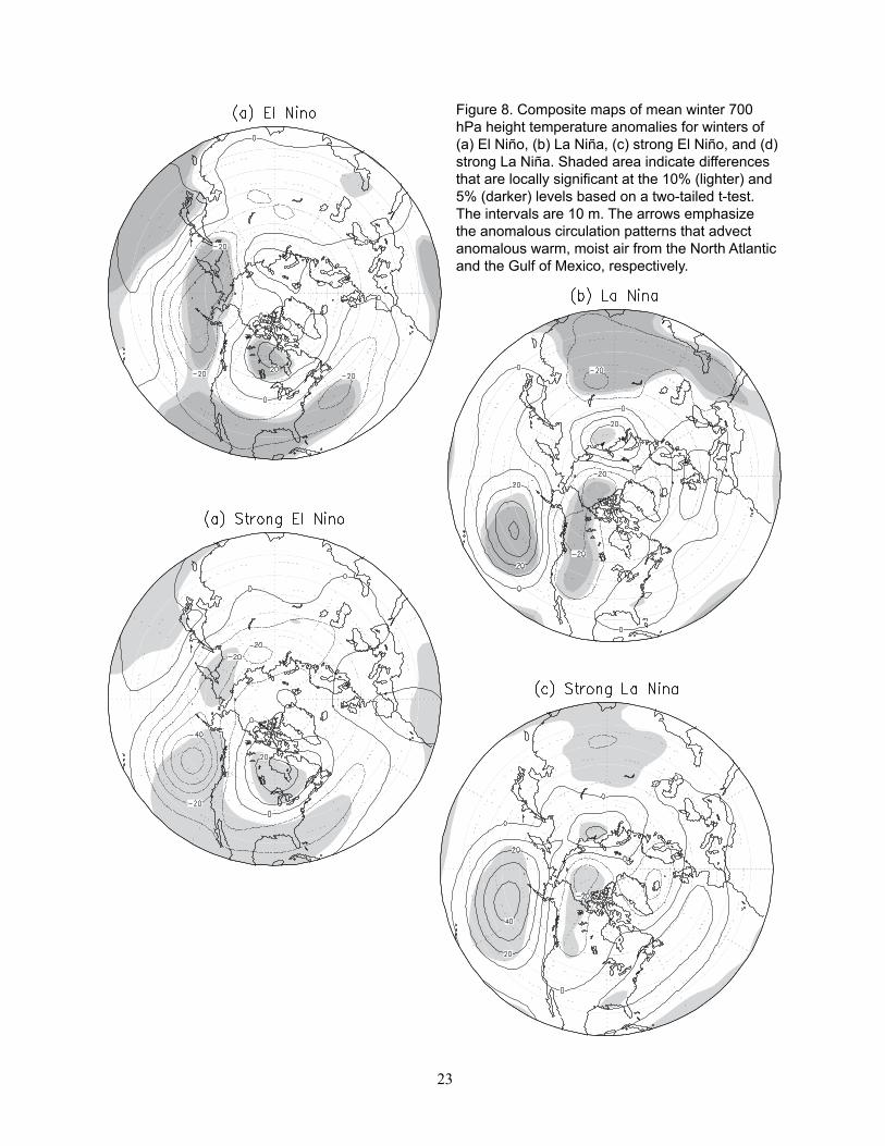
Figure 9. Same as Fig. 8, but for SLP and surface wind anomalies. The SLP intervals are 0.4 hPa. The shaded areas present the 90% significance level .............................................24

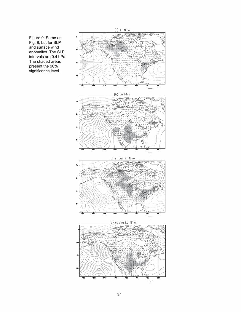
Figure 10. Same as Fig. 8, but for SAT anomalies. The SAT intervals are 0.3°C. The shaded areas present the 90% significance level .................................................................25

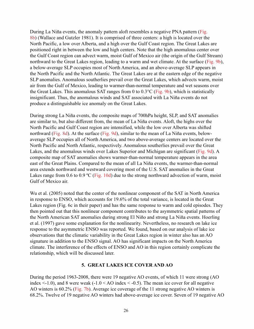
Figure 11. Composite maps of mean winter 700 hPa geopotential height anomalies (relative to AO-neutral mean) for winters of (a) positive and (b) negative AO during 1963-2008. The intervals are 10 m .............................................................................................28

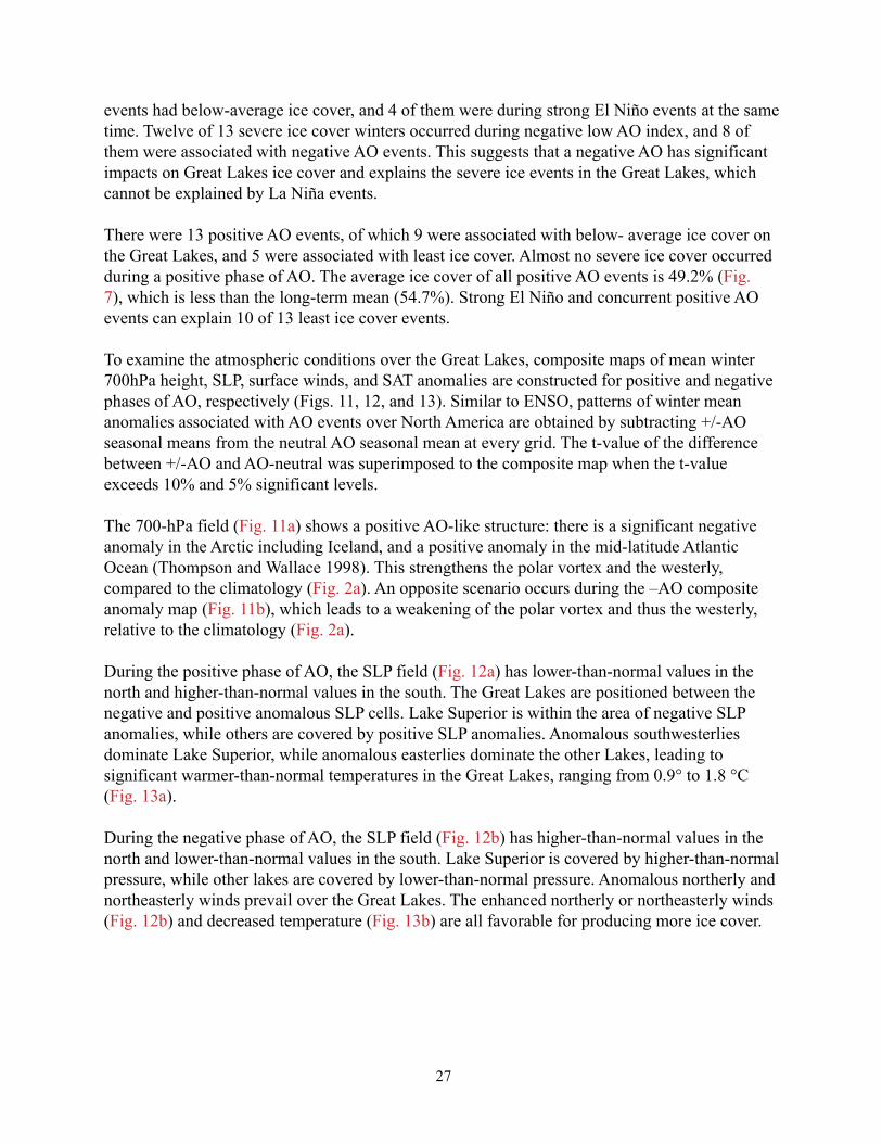
Figure 12. Composite maps of mean winter SLP and surface wind anomalies (relative to AO-neutral mean) for winters of (a) positive and (b) negative AO during 1963-2008. The SLP intervals are 0.4 hPa .....................................................................................................29

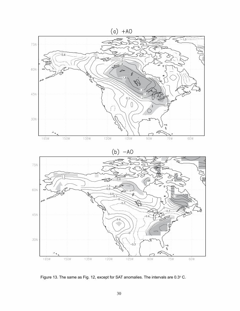
Figure 13. The same as Fig. 12, except for SAT anomalies. The intervals are 0.3°C .................30

Fig. 14. The plane scatter plot of severe (solid) and least (circle) winters with the Nino3.4 index as the x-axis and the AO index as the y-axis .......................................................31

5

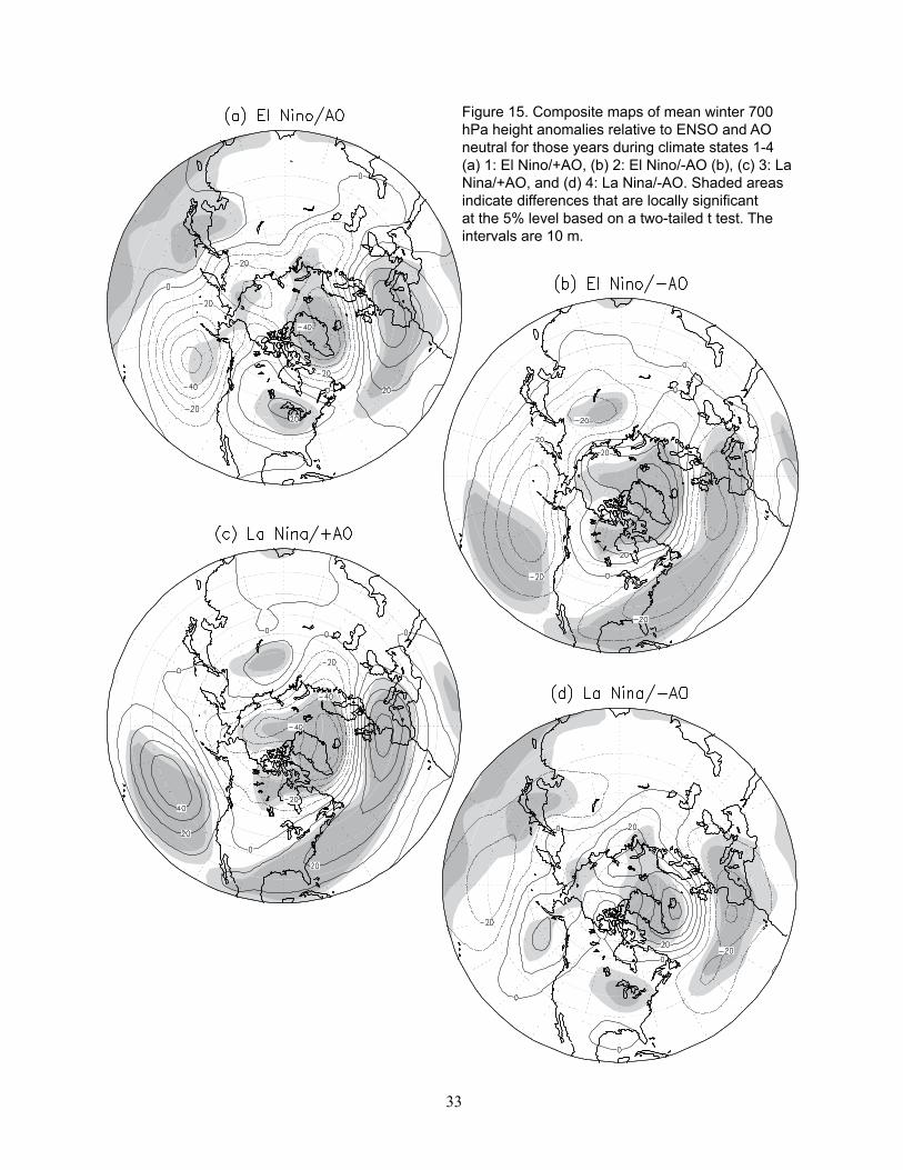
Figure 15. Composite maps of mean winter 700 hPa height anomalies relative to ENSO and AO neutral for those years duing climate states (a) 1: El Nino/+AO, (b) 2: El Nino/-AO,(c) 3: La Nina/+AO, and (d) 4: La Nina/-AO. Shaded areas indicate differences that are locally significant at the 5% level based on a two-tailed t test. The intervals are 10 m .............33

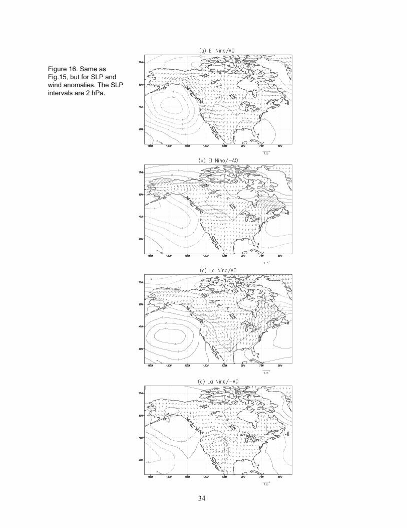
Figure 16. Same as Fig.15, but for SLP and wind anomalies. The SLP intervals are 2 hPa ......34

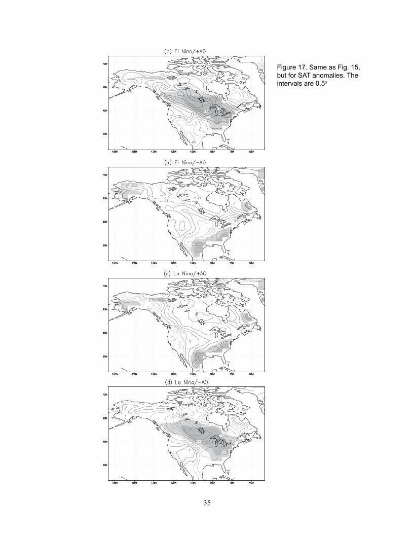
Figure 17. Same as Fig. 15, but for SAT anomalies. The intervals are 0.5°C ............................35

Figure 18. Least ice winter of 1995 during simultaneous El Nino and +AO events (a, state 1) and severe ice winter of 1996 during the simultaneous La Nina and –AO events (b, state 4). The maximum ice cover was 35% and 81%, respectively, significantly different from the climatology of 55% .....................................................................................................................38

Figure 19. Modeled and observed normalized ice coverage for 1963-2008. Black is observations, red is estimated by regression model with Nino3.4 index, square of Nino3.4 index, and AO index as predictors, and blue is estimated by regression model with only Nino3.4 and AO indices as predictors ........................................................................39

LIST OF TABLES

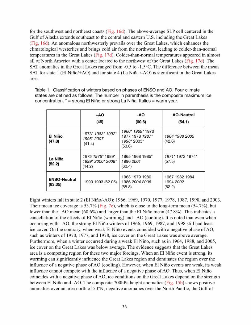
Table 1. Classification of winters based on phases of ENSO and AO. Four climate states are defined as follows. The number in parenthesis is the composite maximum ice concentration. * = strong El Niño or strong La Niña. Italics = warm year ........................................................36

6

7

The Impacts of ENSO and AO/NAO on the Interannual Variability of Great Lakes Ice Cover

Xuezhi Bai, Jia Wang, Cynthia Sellinger, Anne Clites, and Raymond Assel

ABSTRACT. The impacts of El Niño and South Oscillation (ENSO) and Arctic Oscillation (AO) or North Atlantic Oscillation (NAO) on Great Lakes ice cover were investigated using ice observations for winters 1963-2008 and National Centers for Environmental Prediction (NCEP) reanalysis data. Signatures of ENSO and AO/NAO were found in Great Lakes ice cover. However, the impacts are nonlinear and asymmetric. Strong El Niño events are often associated with least ice cover on the Great Lakes, while the impacts of weak El Niño and La Niña events (of all intensities) on the Great Lakes are marginally significant. Negative AO/NAO events are often associated with severe ice cover, while positive AO/NAO events often lead to lower ice cover. The strong El Niño and negative AO/NAO events account for about 50% of the least and severe ice cover winters on the Great Lakes, respectively. The interference of the effects of ENSO and AO/NAO over the Great Lakes makes the relationships complicated. This may be an important cause of nonlinear and asymmetric responses of the regional climate and Great Lakes ice to ENSO and AO/NAO. Based on the cross composite analysis, it is found that during the simultaneous occurrence of El Niño (La Niña) and +AO (-AO) events, Great Lakes ice cover tends to be least (severe).

1. INTRODUCTION

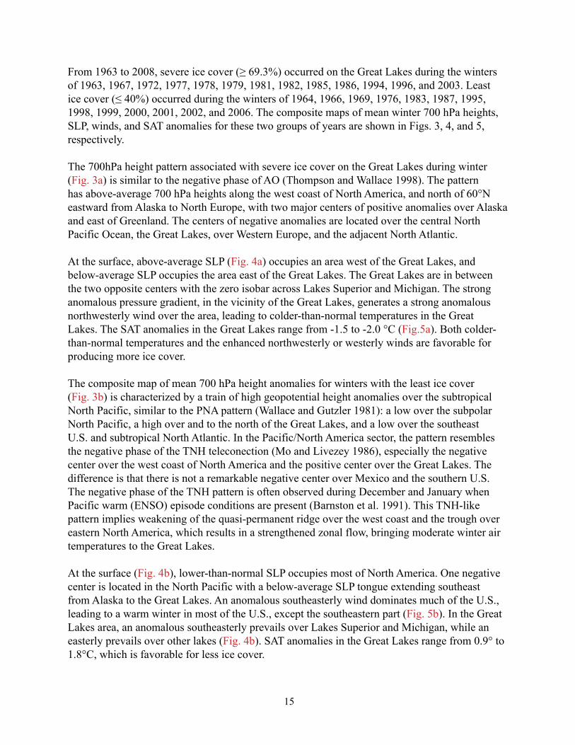
The Laurentian Great Lakes, located in the mid-latitude of eastern North America, contain about 95% of the U.S. and 20% of the world’s fresh surface water supply. Nearly one-eighth of the population of the U.S. and one-third of the population of Canada live within their drainage basin. The ice cover that forms on the Great Lakes each winter affects the regional economy (Niimi 1982). the Lake’s ecosystem (Vanderploeg et al. 1992, Brown et al. 1993, Magnuson et al. 1995), and water level variability (Assel et al. 2004b). For example, from the late 1990s to the early 2000s, lake ice cover was much less than normal, which enhanced evaporation and led to a significant water level drop of as much as 3-4 feet, depending on the lake (Sellinger et al. 2008). Lower water levels have a significant impact on the Great Lakes economy. Over 200 million tons of cargo are shipped every year through the Great Lakes. Since 1998 when water levels took a severe drop, commercial ships were forced to light-load their vessels. For every inch of clearance that these oceangoing vessels lost due to low water levels, they each lost $11,000-22,000 in profits depending on the cargo. Hydropower plants have also been affected by low water levels; several New York and Michigan plants were run at less than capacity, forcing them to buy higher priced energy from other sources, and thereby passing on the higher costs to consumers.

Lake ice cover is also a sensitive indicator of regional climate and climate change (Smith 1991, Hanson et al. 1992, Assel and Robertson 1995, Assel et al. 2003). Seasonal ice cover repeats

8

each year with large interannual variability. For example, the maximum ice coverage was 95% in 1979 and only 11% in 2002. Possible contributors include interannual and interdecadal climate variability, and long-term trends, possibly related to global climate change. The relationship between interannual variability of ice cover on the Great Lakes and large scale atmospheric circulation has been studied. Studies show that teleconnection patterns such as the Pacific/North America (PNA), the Tropical-North Hemisphere (TNH), the NAO, the Polar/Eurasian (POL), and the West Pacific (WP) etc., are associated with anomalous ice cover on the Great Lakes (Assel and Rodionov 1998, Assel et al. 2003, Rodionov and Assel 2000, 2003). Combinations of threshold values (both positive and negative) of the POL, PNA, and TNH indices accounted for much of the interannual variation of winter severity, while threshold values of the Multivariate ENSO index and the TNH index were found to be useful in modeling Great Lakes annual maximum ice cover variations. A 30-day ice forecast model has been developed using linear regression, with teleconnection indices as input (Assel et al. 2004a).

The impacts of ENSO and NAO on Great Lakes ice cover were investigated. Assel and Rodionov (1998) pointed out that ice cover tends to be below average during El Niño events, but association between La Niña events and cold winters (above average ice cover) in the Great Lakes basin is much weaker and less stable. Rodionov and Assel (2000, 2003) found that the relationship between ENSO and severity of winters in the Great Lakes is highly nonlinear. Strong El Niño events are associated with warmth in the Great Lakes region, and the stronger the event, the milder the winter. The Pacific Decadal Oscillation (PDO) is found to modulate the effect of the ENSO on the Great Lakes Winter Severity Index (WSI) (Rodionov and Assel 2003). The correlation between ENSO and WSI is weak (-0.13) during the cold phase of PDO and strong (0.70) during the warm PDO phase. During the warm phase of PDO without a strong ENSO, winters are colder. This occurred in the late 1970s and early 1980s and was responsible for a high ice cover regime during those years. Assel and Rodionov (1998) found that the negative mode of the NAO appears to be associated with above-average ice cover on the Great Lakes. Great Lakes ice cover tends to be below average with a positive NAO mode.

AO (Thompson and Wallace 1998; Wang and Ikeda 2000) and ENSO are the leading modes of interannual climate variability in the northern hemisphere. ENSO is the dominant mode in the tropics, while AO dominates in the high latitudes. Both ENSO and AO have large impacts on the climate of North America including the Great Lakes area.

Many researchers have documented ENSO signals in North American temperatures since the 1980s (Ropelewski and Halpert 1986, Kiladis and Diaz 1989, Halpert and Ropelewski 1992, Gershunov and Barnett 1998). The well-known pattern, associated with El Niño, features above-normal surface air temperature (SAT) along the west coast of North America and western and central Canada; and below-normal SAT in the southern U.S. and the Gulf of Mexico. This distribution of SAT anomalies is often explained by the PNA type of atmospheric circulation present during El Niño events.

Recent evidence from observational studies and numerical models show that North American climate has asymmetric response patterns to the opposite phases of ENSO (Livezey et al. 1997, Hoerling et al. 1997, 2001, Wu et al. 2005). Using neural networks, Wu et al. (2005) examined

9

the nonlinear patterns of North American winter temperature associated with ENSO. They found that the active center of the asymmetries between warm and cold events are almost prominent near the Great Lakes, making this region particularly interesting for studying the mechanism of the ENSO effect on North American climate.

The extratropical atmospheric response to El Niño in a northern winter is manifested by the Pacific-North American (PNA) teleconnection pattern, which can be found simply by linear regression or correlation analysis (Wallace and Gutzler 1981, Horel and Wallace 1981), and is rather well explained by linear wave propagation theory (Hoskins and Karoly 1981). The PNA pattern accounts for a considerable part of the variance of interannual climate fluctuations over the North Pacific (NP) and North America and is regarded as a major source of skill for seasonal forecasts (e.g. Zwiers 1987, Barnston 1994, Shabbar and Barnston 1996, Derome et al. 2001).

Besides the PNA, the TNH, WP, and NP are also associated with changes in sea surface temperature (SST) in the tropical Pacific (Mo and Livezey 1986, Trenberth et al. 1998). The PNA, WP, and TNH exist in winter, while the NP applies to the March-May season. An individual pattern, therefore, cannot represent all of ENSO’s influences.

The AO was defined by Thompson and Wallace (1998) as the leading empirical orthogonal function (EOF) mode of wintertime sea level pressure (SLP) anomalies over the extratropical Northern Hemisphere. The AO is the primary mode of wintertime variability over the extratropical Northern Hemisphere (NH) on timescales ranging from intraseasonal to interdecadal. The AO incorporates many of the features of the associated, more localized NAO (Hurrell 1996, Hurrell and van Loon 1997), but its larger horizontal scale and higher degree of zonal symmetry render it more like a surface signature of the polar vortex aloft. The correlation between the AO and NAO is about 0.84. The AO accounts for a substantially larger fraction of the variance of NH surface air temperature than the NAO. Hodges (2000) showed that, in the positive phase of AO, lower-than-normal atmospheric pressure over the Arctic induces strong westerly winds in the upper atmosphere at northern latitudes, which keeps cold Arctic air to the north, leading to a warmer winter in much of the U.S., east of the Rocky Mountains, and central Canada. In the negative phase of AO, higher-than-normal SLP over the Arctic induces weaker westerly winds in the upper atmosphere, which allows cold Arctic air to reach more southerly latitudes, resulting in a colder winter in the U.S., but warmer weather in northeastern Canada. Wu et al. (2006) studied the nonlinear association between the AO and North America winter climate and found that the linear component is dominate in the Atlantic sector, while the nonlinear component becomes increasingly important in the Pacific-West Coast area.

Geographically, the Great Lakes are located at the edge of two important centers of action, or teleconnections, affecting the North America climate: the PNA and the AO/NAO. These two patterns play a very important role in interannual variability of the U.S. climate. However, their impacts on Great Lakes ice cover may be marginally significant.

The Great Lakes are located between the Alberta High and the southeastern U.S. low of the PNA pattern, close to the nodal point of this oscillation. Any distortion of the pattern and shift of the centers may result in different responses in the winter temperature and ice cover. Thus, this index

10

may not be a good classifier for the winter severity in the Great Lakes (Rodionov and Assel, 2000). The Great Lakes are located at the western edge of the influence of the Icelandic Low, one of the action centers of the AO/NAO. Although it is influenced by the Icelandic Low, whose intensity is associated with AO/NAO (+/-AO means a stronger/weaker Icelandic low), ice cover response may vary with any displacement of the Icelandic Low (Wang et al. 2010).

Some studies seeking to find a significant relationship between ice cover and various teleconnection patterns found that some climate patterns are not independent, such as the PNA and the TNH, but instead are both influenced by ENSO. Based on these previous studies, a linear regression model was developed to forecast ice cover using Beginning of Month (BOM) data with a 30-day lead. Predictors include Accumulated Freezing Degree Day (AFDD) and indices of the atmospheric circulation, such as TNH, SOI, East Atlantic, Western Russia (EAWR), POL, and East Pacific (EP), etc. The perfect AFDD model, which uses observed values of AFDD for the month between the forecast issue date and the forecast date instead of predicted AFDD, has the highest overall forecast skill; however, it requires an accurate 30-day air temperature forecast (Assel et al. 2004a). If the relationship is nonlinear, this linear model cannot reflect the linkage and therefore, is difficult to make an accurate prediction. The methods used in previous studies such as classification and regression tree analysis provided some insight into physical mechanisms (atmospheric circulation characteristics) underlying the statistical relationships identified in the models (Rodionov et al. 2001). Therefore, it is necessary to provide improved, physically sound explanations of dynamic mechanisms.

Although both ENSO and AO/NAO have impacts on Great Lakes ice cover, due to the geographic location of the Great Lakes, their impacts may not always be significant. The interference of ENSO and AO/NAO complicates the relationship between Great Lakes ice cover and ENSO or AO/NAO. This makes forecasting ice cover a great challenge. This study aims to investigate the individual impacts of ENSO and AO/NAO on Great Lakes ice cover and to further examine their combined effects. Differing from previous studies, we focus on the combined effects of both ENSO and AO/NAO on lake ice cover and search for practical predictors of lake ice variability, based on the nonlinear nature of ENSO and the interference of ENSO and AO/NAO.

This paper is organized as follows. The data and the methods are briefly introduced in Section 2. The atmospheric conditions for severe and least ice cover are presented in Section 3. The relationships between Great Lakes ice cover and ENSO and AO/NAO are discussed in Sections 4 and 5, respectively. In Section 6, the interference and combined effects of ENSO and AO/NAO are investigated. Section 7 presents both linear and nonlinear regression models for predicting lake ice using both ENSO and AO/NAO indices. Lastly, Section 8 summarizes the results.

2. DATA AND METHODS

2.1 Winter maximum ice cover

Systematic lake-scale observations of Great Lakes ice cover began in the 1960s by federal agencies in the U.S. (U.S. Army Corps of Engineers and U.S. Coast Guard) and Canada

11

(Atmospheric Environment Service and Canadian Coast Guard) to support early and late season navigation, the closing of the navigation season in winter, and the opening of navigation in spring. Observations were made at irregular intervals primarily to support operational activities. Ice charts depicting ice concentration patterns and ice extent were constructed from satellite imagery, side-looking airborne radar imagery, and visual aerial ice reconnaissance (Assel and Rodionov 1998).

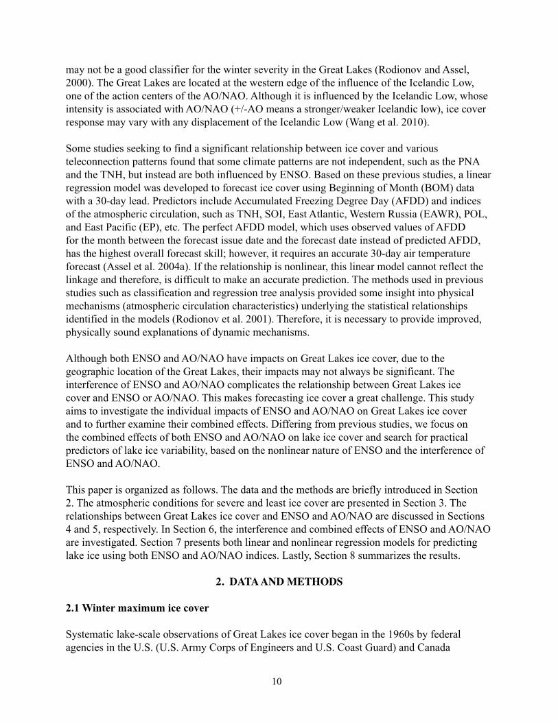
Winter (December-March) maximum ice coverage (WMIC) is defined as the greatest percentage of ice coverage, by surface area, each winter for the Great Lakes. WMIC data for winters 1963-2008 were constructed using analysis of ice charts obtained from the National Ice Center and the Canadian Ice Service (Assel et al. 2003) (Fig. 1a). The long-term mean (1963-2008) WMIC is 54.7%, and the standard deviation is 20.9%. In this analysis, winters with normalized WMIC

Figure 1 (a) 1963-2008 Great Lakes winter maximum ice coverage. (b) Time series of winter AO and ENSO indices from 1963 to 2008. The zero-lag correlations are also calculated: r(AO, ice)=-0.28, r(Nino3.4, ice)=-0.18, r(Nino3.42, ice)=-0.45.

12

greater than or equal to 0.7 (≥ 69.3%) were identified as severe ice cover winters, and winters with normalized WMIC less than or equal to -0.7 (≤ 40%) were identified as least ice cover winters.

2.2 NCEP/NCAR reanalysis

We used monthly reanalysis data from the National Center of Environmental Prediction/National Centers of Atmospheric Research (NCEP) (Kalnay et al. 1996) to investigate the relationship between Great Lakes ice and atmosphere circulation anomalies. The data are available from 1948 to present. The resolution is 2.5×2.5 degrees. The climatology of the period 1948-2007 was calculated, and monthly anomalies were obtained by subtracting the climatology from the individual months. Average (December-January-February, DJF) anomalies were calculated for each winter: 1949 (December 1948, January 1949, February 1949), 1950 (December 1949, January 1950, and February 1950), and so on to 2008 (December 2007, January 2008, and February 2008). In this study, surface air temperature (SAT), sea level pressure (SLP), surface winds, and 700 hPa geopotential heights were used.

2.3 Climate indices

We use the Nino3.4 SST (Sea Surface Temperature) anomaly index as a marker of ENSO variability and identify the warm and cold episodes during 1950-2008 based on a threshold of +/- 0.5oC. Cold and warm episodes are defined when the threshold is met for a minimum of five consecutive over-lapping seasons. Otherwise, the winter is defined as ENSO-Neutral. The index is defined as 3-month running mean of ERSST.v3 (Extended Reconstructed Sea Surface Temperature Version 3) SST anomalies in the Niño3.4 region (5oN-5oS, 120o-170oW; obtained from NOAA/CPC (Climate Prediction Center) http://www.cpc.noaa.gov/products/analysis monitoring/ensostuff/ensoyears.shtml). The strong warm (cold) winters are defined when the DJF (Dec-Jan-Feb) mean index exceeds 1.0 (-1.0), and weak ones are defined when the DJF mean index is greater than 0.5, but less than 1.0.

The monthly AO index from 1950 to 2008 was obtained from NOAA/CPC (http://www.cpc.noaa.gov/products/precip/CWlink/daily_ao_index/ao_index.html). The AO is defined as the first leading mode from the EOF analysis of monthly mean height anomalies at 1000-hPa. Monthly AO indices are constructed by projecting the monthly mean 1000-hPa height anomalies onto the leading EOF mode.

The AO index is standardized, and a winter is defined as a positive (negative) phase when the DJF mean index exceeds the +0.5 (-0.5) standard deviation, otherwise a winter is defined as AO-neutral. Figure 1b shows both DJF mean Nino3.4 and AO indices for the period 1963-2008.

2.4 Methods

The methods used in this study are correlation analysis and composite analysis. Composite analysis is a common way to present the responses associated with a certain climate event such as ENSO and AO by averaging the data over the years when the certain event occurred. Due

13

to the small samples available in this study, the Student’s t-distribution was used to determine the statistical significance between the means of the two samples. Comparing the differences between the two means using the Students t-test requires two independent samples of sizes n1 and n2, which possess means and standard deviations given by 1x and 2x and 1s and 2s , respectively. Our null hypothesis, H0, is when the two samples are statistically indistinguishable from each other. To test H0, we use the conventional t-score

+•

−+−+−

−=

2121

222

211

21

112

)1()1(nnnn

snsn

xxt (1)

which is a value of a random variable having a t-distribution with n1+n2-2 degrees of freedom. The null hypothesis is rejected if the two-tailed t-score exceeds the 90% confidence interval.

3. CLIMATOLOGY, COMPOSITE ATMOSPHERIC CONDITIONS FOR SEVERE AND LEAST ICE COVER

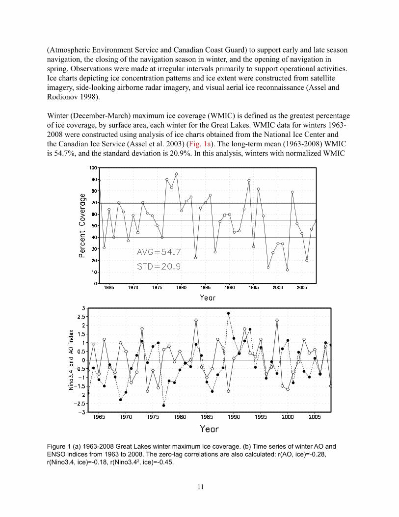
To help interpret an anomaly of any variable, we first construct the climatology of 700 hPa height (Fig. 2a), SLP and wind (Fig. 2b), and SAT (Fig. 2c) fields for the period 1948-2008. A variable (say SAT, T) can be decomposited into a time-mean climatology and an anomaly:

€

T(x,y,z;t) = T(x,y,z) + T '(x,y,z;t) , where the bar denotes the time-mean climatology, the prime means the anomaly departing from the climatology, and (x, y, z; t) denotes the longitude, latitude, height, and time, respectively.

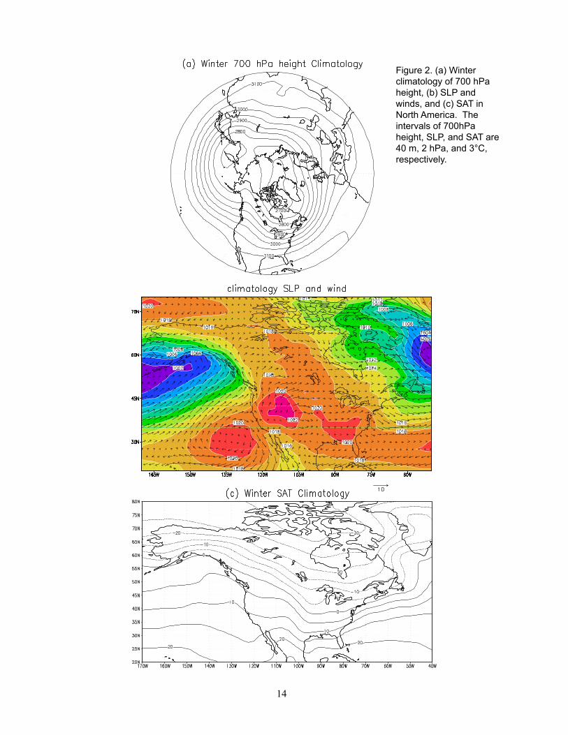
The climatological 700-hPa height field (Fig. 2a) indicates a polar vortex structure with a ridge-trough system over North America. The ridge line extends from Alaska to the Rocky Mountains, while the trough line extends from Hudson Bay to the Great Lakes region. The westerly dominates over the mid-latitudes at around 40°N.

The climatological SLP field (Fig. 2b) is featured by the Iceland and Aleutian Lows, a subtropical high occupied in the U.S. continent, and the Beaufort High in the Arctic. The climatological surface wind patterns are the cyclonic circulations in the North Pacific associated with the Aleutian Low and in the North Atlantic related to the Icelandic Low. Westerlies dominate the Great Lakes region. It is well-known that the subpolar lows and the subpolar high over North America are due to a land-sea temperature contrast during winter seasons. Thus, the winter SLP, similar to the 700-hPa height, has a large trough in the North Pacific and North Atlantic, respectively, and has a ridge in the U.S. continent.

The climatological SAT field (Fig. 2c) shows the higher temperature in the subpolar oceans and lower temperature over the U.S., consistent with the SLP field due to land-sea temperature contrast. In the Great Lakes region, climatological SAT ranges from -3°C in Lake Erie to -12°C in northern Lake Superior.

14

Figure 2. (a) Winter climatology of 700 hPa height, (b) SLP and winds, and (c) SAT in North America. The intervals of 700hPa height, SLP, and SAT are 40 m, 2 hPa, and 3°C, respectively.

15

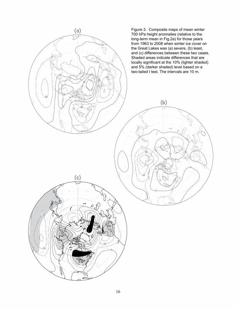
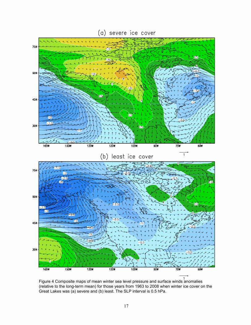
From 1963 to 2008, severe ice cover (≥ 69.3%) occurred on the Great Lakes during the winters of 1963, 1967, 1972, 1977, 1978, 1979, 1981, 1982, 1985, 1986, 1994, 1996, and 2003. Least ice cover (≤ 40%) occurred during the winters of 1964, 1966, 1969, 1976, 1983, 1987, 1995, 1998, 1999, 2000, 2001, 2002, and 2006. The composite maps of mean winter 700 hPa heights, SLP, winds, and SAT anomalies for these two groups of years are shown in Figs. 3, 4, and 5, respectively.

The 700hPa height pattern associated with severe ice cover on the Great Lakes during winter (Fig. 3a) is similar to the negative phase of AO (Thompson and Wallace 1998). The pattern has above-average 700 hPa heights along the west coast of North America, and north of 60°N eastward from Alaska to North Europe, with two major centers of positive anomalies over Alaska and east of Greenland. The centers of negative anomalies are located over the central North Pacific Ocean, the Great Lakes, over Western Europe, and the adjacent North Atlantic.

At the surface, above-average SLP (Fig. 4a) occupies an area west of the Great Lakes, and below-average SLP occupies the area east of the Great Lakes. The Great Lakes are in between the two opposite centers with the zero isobar across Lakes Superior and Michigan. The strong anomalous pressure gradient, in the vicinity of the Great Lakes, generates a strong anomalous northwesterly wind over the area, leading to colder-than-normal temperatures in the Great Lakes. The SAT anomalies in the Great Lakes range from -1.5 to -2.0 °C (Fig.5a). Both colder-than-normal temperatures and the enhanced northwesterly or westerly winds are favorable for producing more ice cover.

The composite map of mean 700 hPa height anomalies for winters with the least ice cover (Fig. 3b) is characterized by a train of high geopotential height anomalies over the subtropical North Pacific, similar to the PNA pattern (Wallace and Gutzler 1981): a low over the subpolar North Pacific, a high over and to the north of the Great Lakes, and a low over the southeast U.S. and subtropical North Atlantic. In the Pacific/North America sector, the pattern resembles the negative phase of the TNH teleconection (Mo and Livezey 1986), especially the negative center over the west coast of North America and the positive center over the Great Lakes. The difference is that there is not a remarkable negative center over Mexico and the southern U.S. The negative phase of the TNH pattern is often observed during December and January when Pacific warm (ENSO) episode conditions are present (Barnston et al. 1991). This TNH-like pattern implies weakening of the quasi-permanent ridge over the west coast and the trough over eastern North America, which results in a strengthened zonal flow, bringing moderate winter air temperatures to the Great Lakes.

At the surface (Fig. 4b), lower-than-normal SLP occupies most of North America. One negative center is located in the North Pacific with a below-average SLP tongue extending southeast from Alaska to the Great Lakes. An anomalous southeasterly wind dominates much of the U.S., leading to a warm winter in most of the U.S., except the southeastern part (Fig. 5b). In the Great Lakes area, an anomalous southeasterly prevails over Lakes Superior and Michigan, while an easterly prevails over other lakes (Fig. 4b). SAT anomalies in the Great Lakes range from 0.9° to 1.8°C, which is favorable for less ice cover.

16

Figure 3. Composite maps of mean winter 700 hPa height anomalies (relative to the long-term mean in Fig.2a) for those years from 1963 to 2008 when winter ice cover on the Great Lakes was (a) severe, (b) least, and (c) differences between these two cases. Shaded areas indicate differences that are locally significant at the 10% (lighter shaded) and 5% (darker shaded) level based on a two-tailed t test. The intervals are 10 m.

17

Figure 4 Composite maps of mean winter sea level pressure and surface winds anomalies (relative to the long-term mean) for those years from 1963 to 2008 when winter ice cover on the Great Lakes was (a) severe and (b) least. The SLP interval is 0.5 hPa.

18

Fig. 5 Composite maps of mean winter surface air temperature anomalies (relative to the long-term mean) for those years from 1963 to 2008 when winter ice cover on the Great Lakes was (a) severe, (b) least, and (c) differences between these two cases. In (c), shaded areas indicate differences that are locally significant at the 10% (lighter) and 5% (darker) level based on a two-tailed t test. The intervals are 0.3 oC in (a) and (b), and 1 oC in (c)

19

The difference between the composite 700hPa heights and SAT for severe and least ice cover was constructed (Figs. 3c and 5c). Significant negative difference centers are located in the subtropical belt, in the vicinity of the Great Lakes (negative), and in Europe (positive, Fig. 3c). Centers of significant positive differences are located over Alaska and just east of Greenland. The temperature difference between a severe and least ice cover winter ranges from -2.5 to -4 °C in the Great Lakes. The significant difference is over the northeast U.S. and southern Canada with the Great Lakes near its center. It is found from the composite analysis that both AO and ENSO have impacts on Great Lakes ice cover. The atmospheric circulation pattern for severe ice cover resembles a mixture of a negative phase of AO and a positive PNA pattern. The atmospheric pattern for least ice cover resembles a negative phase of TNH, which is often observed during El Niño events. There are eight –AO years in the group of severe ice cover, and seven El Niño years in the group of least ice cover.

4. GREAT LAKES ICE COVER AND ENSO

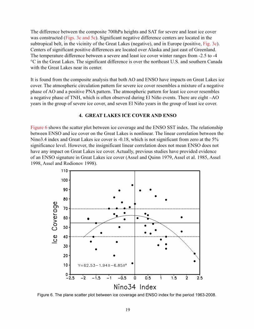
Figure 6 shows the scatter plot between ice coverage and the ENSO SST index. The relationship between ENSO and ice cover on the Great Lakes is nonlinear. The linear correlation between the Nino3.4 index and Great Lakes ice cover is -0.18, which is not significant from zero at the 5% significance level. However, the insignificant linear correlation does not mean ENSO does not have any impact on Great Lakes ice cover. Actually, previous studies have provided evidence of an ENSO signature in Great Lakes ice cover (Assel and Quinn 1979, Assel et al. 1985, Assel 1998, Assel and Rodionov 1998).

Figure 6. The plane scatter plot between ice coverage and ENSO index for the period 1963-2008.

20

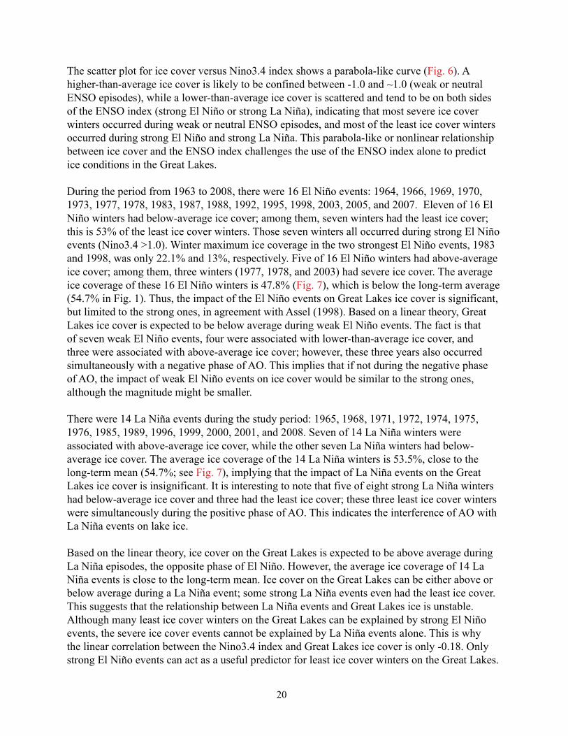
The scatter plot for ice cover versus Nino3.4 index shows a parabola-like curve (Fig. 6). A higher-than-average ice cover is likely to be confined between -1.0 and ~1.0 (weak or neutral ENSO episodes), while a lower-than-average ice cover is scattered and tend to be on both sides of the ENSO index (strong El Niño or strong La Niña), indicating that most severe ice cover winters occurred during weak or neutral ENSO episodes, and most of the least ice cover winters occurred during strong El Niño and strong La Niña. This parabola-like or nonlinear relationship between ice cover and the ENSO index challenges the use of the ENSO index alone to predict ice conditions in the Great Lakes. During the period from 1963 to 2008, there were 16 El Niño events: 1964, 1966, 1969, 1970, 1973, 1977, 1978, 1983, 1987, 1988, 1992, 1995, 1998, 2003, 2005, and 2007. Eleven of 16 El Niño winters had below-average ice cover; among them, seven winters had the least ice cover; this is 53% of the least ice cover winters. Those seven winters all occurred during strong El Niño events (Nino3.4 >1.0). Winter maximum ice coverage in the two strongest El Niño events, 1983 and 1998, was only 22.1% and 13%, respectively. Five of 16 El Niño winters had above-average ice cover; among them, three winters (1977, 1978, and 2003) had severe ice cover. The average ice coverage of these 16 El Niño winters is 47.8% (Fig. 7), which is below the long-term average (54.7% in Fig. 1). Thus, the impact of the El Niño events on Great Lakes ice cover is significant, but limited to the strong ones, in agreement with Assel (1998). Based on a linear theory, Great Lakes ice cover is expected to be below average during weak El Niño events. The fact is that of seven weak El Niño events, four were associated with lower-than-average ice cover, and three were associated with above-average ice cover; however, these three years also occurred simultaneously with a negative phase of AO. This implies that if not during the negative phase of AO, the impact of weak El Niño events on ice cover would be similar to the strong ones, although the magnitude might be smaller.

There were 14 La Niña events during the study period: 1965, 1968, 1971, 1972, 1974, 1975, 1976, 1985, 1989, 1996, 1999, 2000, 2001, and 2008. Seven of 14 La Niña winters were associated with above-average ice cover, while the other seven La Niña winters had below-average ice cover. The average ice coverage of the 14 La Niña winters is 53.5%, close to the long-term mean (54.7%; see Fig. 7), implying that the impact of La Niña events on the Great Lakes ice cover is insignificant. It is interesting to note that five of eight strong La Niña winters had below-average ice cover and three had the least ice cover; these three least ice cover winters were simultaneously during the positive phase of AO. This indicates the interference of AO with La Niña events on lake ice.

Based on the linear theory, ice cover on the Great Lakes is expected to be above average during La Niña episodes, the opposite phase of El Niño. However, the average ice coverage of 14 La Niña events is close to the long-term mean. Ice cover on the Great Lakes can be either above or below average during a La Niña event; some strong La Niña events even had the least ice cover. This suggests that the relationship between La Niña events and Great Lakes ice is unstable. Although many least ice cover winters on the Great Lakes can be explained by strong El Niño events, the severe ice cover events cannot be explained by La Niña events alone. This is why the linear correlation between the Nino3.4 index and Great Lakes ice cover is only -0.18. Only strong El Niño events can act as a useful predictor for least ice cover winters on the Great Lakes.

21

Figure 7. Average winter maximum ice coverage for (a) ENSO, (b) AO, and (c) four climate states.

(a)

(b)

(c)

Mean

Mean

Mean

22

This asymmetric response of Great Lakes ice to ENSO is consistent with the finding that the impacts of ENSO on lakes ice cover (Assel 1998) and on North America climate is nonlinear (Livezey et al. 1997, Hoerling et al. 1997, 2001, Wu et al. 2005).

In the following, we investigate the atmospheric conditions in El Niño and La Niña events with a focus on the Great Lakes. Patterns of winter mean anomalies associated with ENSO events over North America are obtained by subtracting El Niño (La Niña) seasonal means from the neutral ENSO seasonal mean at every grid. The t-value of the difference between the El Niño (La Niña) and ENSO-neutral means was computed and superimposed in the composite map when the t-value exceeds 10% and 5% significance levels.

The composite map of winter 700hPa height anomalies for the 16 El Niño events shows positive anomalies over Canada and the northern U.S. with a center located over Hudson Bay (Fig. 8a). Significant negative anomalies are located over the subpolar Pacific, Mexico, and the southern U.S. Note that anomalous northeasterly winds associated with the negative anomalous center off the U.S. east coast can advect warm, moist air over the Atlantic Gulf Stream to the northeastern U.S. and the Great Lakes region, leading to heavy precipitation. At the surface (Fig. 9a), the entire U.S. was occupied by below-average SLP. Two negative SLP centers are located in the subpolar Pacific and North Atlantic, respectively. The negative SLP center in the North Atlantic produces an anomalous northeasterly, bringing warm, moist Atlantic air to the northeastern U.S. An anomalous easterly prevails over Lakes Superior and Michigan, while a northerly prevails over Lakes Huron, Ontario, and Erie. Warmer-than-normal temperature appears over the northern U.S. and most of Canada (Fig. 10a), while colder-than-normal temperature occupies Mexico and the southern U.S. A warm tongue extends southeastward from Alaska to the Great Lakes. The SAT anomalies in the Great Lakes range from 0°C to 1.2°C, decreasing from north to south, indicating that the upper Lakes are affected more by El Niño than the lower Lakes. Both weakened westerly and warmer-than-normal temperature is favorable for less ice cover on the Great Lakes.

The composite map of winter 700hPa height anomalies for nine strong El Niño events shows a clear negative TNH signature (Fig. 8c). It consists of three centers: a low off the west coast of North America, a high near the Great Lakes region, and a low over the southeastern U.S. The above-average 700hPa heights over the Great Lakes and below-average heights centered off the west coast of North America are responsible for the flattening of the ridge-trough system (Fig. 2a) over North America, which prevents a cold air mass from intruding from the north, leading to warmer-than-normal temperature over almost the entire U.S. At the surface (Fig. 9c), two centers of negative SLP anomalies are located in the North Pacific off the west coast of North America, and North Atlantic off the southeast coast of the U.S., respectively. Northeast Canada and part of the northeastern U.S. including most of the Great Lakes are covered by above-average SLP. Anomalous easterly and southeasterly winds prevail over Lake Superior and northern Lake Michigan, while anomalous northerly and northeasterly winds prevail over the other lakes. Except for the southwest region, almost the entire U.S. is warmer than normal with a significant area in the vicinity of the Great Lakes (Fig. 10c). The SAT anomalies in the Great Lakes range from 0.9 to 2.1°C, which are significant relative to the neutral mean.

23

Figure 8. Composite maps of mean winter 700 hPa height temperature anomalies for winters of (a) El Niño, (b) La Niña, (c) strong El Niño, and (d) strong La Niña. Shaded area indicate differences that are locally significant at the 10% (lighter) and 5% (darker) levels based on a two-tailed t-test. The intervals are 10 m. The arrows emphasize the anomalous circulation patterns that advect anomalous warm, moist air from the North Atlantic and the Gulf of Mexico, respectively.

24

Figure 9. Same as Fig. 8, but for SLP and surface wind anomalies. The SLP intervals are 0.4 hPa. The shaded areas present the 90% significance level.

25

Figure 10. Same as Fig. 8, but for SAT anomalies. The SAT intervals are 0.3 °C. The shaded areas present the 90% significance level.

26

During La Niña events, the anomaly pattern aloft resembles a negative PNA pattern (Fig. 8b) (Wallace and Gutzler 1981). It is comprised of three centers: a high is located over the North Pacific, a low over Alberta, and a high over the Gulf Coast region. The Great Lakes are positioned right in between the low and high centers. Note that the high anomalous center over the Gulf Coast region can advect warm, moist Gulf of Mexico air (the origin of the Gulf Stream) northward to the Great Lakes region, leading to a warm and wet climate. At the surface (Fig. 9b), a below-average SLP occupies most of North America, and an above-average SLP appears in the North Pacific and the North Atlantic. The Great Lakes are at the eastern edge of the negative SLP anomalies. Anomalous southerlies prevail over the Great Lakes, which advects warm, moist air from the Gulf of Mexico, leading to warmer-than-normal temperature and wet seasons over the Great Lakes. This anomalous SAT ranges from 0 to 0.3°C (Fig. 9b), which is statistically insignificant. Thus, the anomalous winds and SAT associated with La Niña events do not produce a distinguishable ice anomaly on the Great Lakes.

During strong La Niña events, the composite maps of 700hPa height, SLP, and SAT anomalies are similar to, but also different from, the mean of La Niña events. Aloft, the highs over the North Pacific and Gulf Coast region are intensified, while the low over Alberta was shifted northward (Fig. 8d). At the surface (Fig. 9d), similar to the mean of La Niña events, below-average SLP occupies all of North America, and two above-average centers are located over the North Pacific and North Atlantic, respectively. Anomalous southerlies prevail over the Great Lakes, and the anomalous winds over Lakes Superior and Michigan are significant (Fig. 9d). A composite map of SAT anomalies shows warmer-than-normal temperature appears in the area east of the Great Plains. Compared to the mean of all La Niña events, the warmer-than-normal area extends northward and westward covering most of the U.S. SAT anomalies in the Great Lakes range from 0.6 to 0.9 ºC (Fig. 10d) due to the strong northward advection of warm, moist Gulf of Mexico air.

Wu et al. (2005) noted that the center of the nonlinear component of the SAT in North America in response to ENSO, which accounts for 19.6% of the total variance, is located in the Great Lakes region (Fig. 6c in their paper) and has the same response to warm and cold episodes. They then pointed out that this nonlinear component contributes to the asymmetric spatial patterns of the North American SAT anomalies during strong El Niño and strong La Niña events. Hoerling et al. (1997) gave some explanation for the nonlinearity. Nevertheless, no research on lake ice response to the asymmetric ENSO was reported. We found, based on our analysis of lake ice observations that the climatic variability in the Great Lakes region in winter also has an AO signature in addition to the ENSO signal. AO has significant impacts on the North America climate. The interference of the effects of ENSO and AO in this region certainly complicate the relationship, which will be discussed later.

5. GREAT LAKES ICE COVER AND AO

During the period 1963-2008, there were 19 negative AO events, of which 11 were strong (AO index <-1.0), and 8 were weak (-1.0 < AO index < -0.5). The mean ice cover for all negative AO winters is 60.2% (Fig. 7b). Average ice coverage of the 11 strong negative AO winters is 68.2%. Twelve of 19 negative AO winters had above-average ice cover. Seven of 19 negative AO

27

events had below-average ice cover, and 4 of them were during strong El Niño events at the same time. Twelve of 13 severe ice cover winters occurred during negative low AO index, and 8 of them were associated with negative AO events. This suggests that a negative AO has significant impacts on Great Lakes ice cover and explains the severe ice events in the Great Lakes, which cannot be explained by La Niña events.

There were 13 positive AO events, of which 9 were associated with below- average ice cover on the Great Lakes, and 5 were associated with least ice cover. Almost no severe ice cover occurred during a positive phase of AO. The average ice cover of all positive AO events is 49.2% (Fig. 7), which is less than the long-term mean (54.7%). Strong El Niño and concurrent positive AO events can explain 10 of 13 least ice cover events. To examine the atmospheric conditions over the Great Lakes, composite maps of mean winter 700hPa height, SLP, surface winds, and SAT anomalies are constructed for positive and negative phases of AO, respectively (Figs. 11, 12, and 13). Similar to ENSO, patterns of winter mean anomalies associated with AO events over North America are obtained by subtracting +/-AO seasonal means from the neutral AO seasonal mean at every grid. The t-value of the difference between +/-AO and AO-neutral was superimposed to the composite map when the t-value exceeds 10% and 5% significant levels.

The 700-hPa field (Fig. 11a) shows a positive AO-like structure: there is a significant negative anomaly in the Arctic including Iceland, and a positive anomaly in the mid-latitude Atlantic Ocean (Thompson and Wallace 1998). This strengthens the polar vortex and the westerly, compared to the climatology (Fig. 2a). An opposite scenario occurs during the –AO composite anomaly map (Fig. 11b), which leads to a weakening of the polar vortex and thus the westerly, relative to the climatology (Fig. 2a). During the positive phase of AO, the SLP field (Fig. 12a) has lower-than-normal values in the north and higher-than-normal values in the south. The Great Lakes are positioned between the negative and positive anomalous SLP cells. Lake Superior is within the area of negative SLP anomalies, while others are covered by positive SLP anomalies. Anomalous southwesterlies dominate Lake Superior, while anomalous easterlies dominate the other Lakes, leading to significant warmer-than-normal temperatures in the Great Lakes, ranging from 0.9° to 1.8 °C (Fig. 13a).

During the negative phase of AO, the SLP field (Fig. 12b) has higher-than-normal values in the north and lower-than-normal values in the south. Lake Superior is covered by higher-than-normal pressure, while other lakes are covered by lower-than-normal pressure. Anomalous northerly and northeasterly winds prevail over the Great Lakes. The enhanced northerly or northeasterly winds (Fig. 12b) and decreased temperature (Fig. 13b) are all favorable for producing more ice cover.

28

Figure 11. Composite maps of mean winter 700 hPa geopotential height anomalies (relative to AO-neutral mean) for winters of (a) positive, and (b) negative AO during 1963-2008. The intervals are 10 m.

29

Figure 12. Composite maps of mean winter SLP and surface wind anomalies (relative to AO-neutral mean) for winters of (a) positive and (b) negative AO during 1963-2008. The SLP intervals are 0.4 hPa.

30

Figure 13. The same as Fig. 12, except for SAT anomalies. The intervals are 0.3o C.

31

6. INTERFERENCE OF EFFECTS OF ENSO AND AO ON GREAT LAKES ICE COVER

The above analyses suggest that the Great Lakes are in such a position where both ENSO and AO can have impacts, but neither dominates. For example, even during strong El Niño events, the Great Lakes are still at the edge of the warm tongue that extends southeast from Alaska (Fig. 10a). There are winters with a strong negative AO, which are not associated with severe ice cover such as the winters of 1966, 1969, 1970, and 2001. Winters of 1966, 1969, and 2001 even had least ice cover. Winters of 1966 and 1969 were also during strong El Niño events. The winter of 1970 was during a weak El Niño event, while the winter of 2001 was during a La Niña event.

It is evident that the interference of effects of ENSO and AO on the Great Lakes complicates the relationships. Thus, it is impossible to use only one of these two indices to accurately predict lake ice cover. In the following, we investigate the interference effects of ENSO and AO.

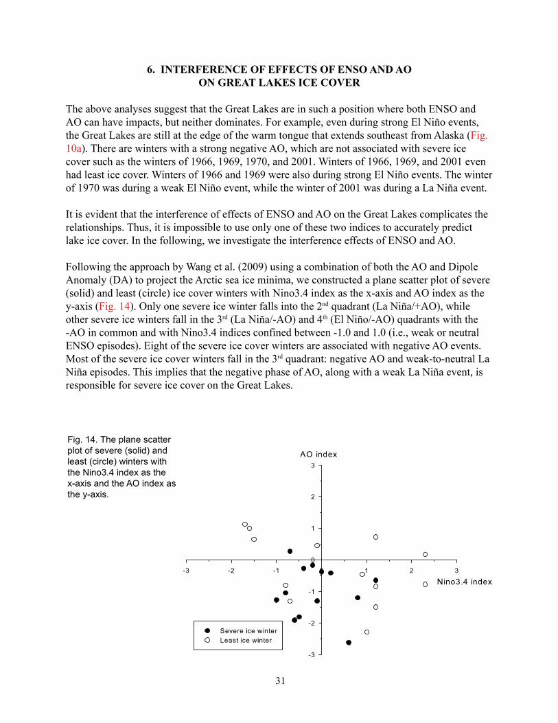
Following the approach by Wang et al. (2009) using a combination of both the AO and Dipole Anomaly (DA) to project the Arctic sea ice minima, we constructed a plane scatter plot of severe (solid) and least (circle) ice cover winters with Nino3.4 index as the x-axis and AO index as the y-axis (Fig. 14). Only one severe ice winter falls into the 2nd quadrant (La Niña/+AO), while other severe ice winters fall in the 3rd (La Niña/-AO) and 4th (El Niño/-AO) quadrants with the -AO in common and with Nino3.4 indices confined between -1.0 and 1.0 (i.e., weak or neutral ENSO episodes). Eight of the severe ice cover winters are associated with negative AO events. Most of the severe ice cover winters fall in the 3rd quadrant: negative AO and weak-to-neutral La Niña episodes. This implies that the negative phase of AO, along with a weak La Niña event, is responsible for severe ice cover on the Great Lakes.

Fig. 14. The plane scatter plot of severe (solid) and least (circle) winters with the Nino3.4 index as the x-axis and the AO index as the y-axis.

32

The least ice cover years are divided into two groups. The first group of seven least years falls in the 1st (El Niño/+AO) and 4th (El Niño/-AO) quadrants, with large positive Nino3.4 index (strong El Niño), regardless of the sign of AO. This indicates that the strong El Niño events dominate. The second group of three years falls in the 2nd quadrant (La Niña/+AO) with a positive AO and negative Nino3.4 index larger than -1 (strong La Niña). Six out of 13 years with least ice cover occurred during the positive phases of AO. Thus, it suggests that a strong El Niño and positive AO are responsible for the least ice cover on the Great Lakes. The combined strong La Niña and positive AO seems also to induce the least ice cover. The evidence also indicates the non-linearity of ENSO effects (see also Fig. 6).

To demonstrate the combined effects of AO and ENSO, the winters were classified into nine groups based on phases of ENSO and AO (see Table 1; Wang et al. 2009). We mainly examined the four climate states: (1) El Niño /+AO, (2) El Niño /-AO, (3) La Niña /+AO, and (4) La Niña /-AO. In general, as discussed in Sections 4 and 5, the Great Lakes tend to be warmer than normal and have less ice cover during El Niño events or a positive phase of AO, and are colder than normal during a negative phase of AO or La Niña events that have weaker impacts on lake ice, compared to the El Niño events (i.e., the asymmetric influence). Thus, when a winter falls during +AO and El Niño episodes (state 1), it is expected to be warmer and have less ice cover, since +AO and El Niño have the same warming effect on the Great Lakes. When a winter falls during –AO and La Niña at the same time (state 4), it is expected to be colder and have more ice cover. Furthermore, if a winter happens to be in the state of El Niño/-AO (state 2) or La Niña/+AO (state 3), the cancellation of the two opposite effects (ENSO and AO) will complicate the relationship.

During 1963-2008, five winters fall into state 1 (El Niño /+AO): 1973, 1983, 1992, 1995, and 2007. The average ice coverage for these winters is 41.4% (Fig. 7c), which is well below the long-term mean (54.7%), and is also lower than the mean ice cover of all El Niño winters (47.8%). Except for 1973 (60.6%), all winters had lower-than-average ice cover, and winters of 1983 (22.1%) and 1995 (32%) have least ice cover. The mean 700hPa height anomalies (Fig. 15a) of these five winters clearly indicates +AO and El Niño signatures with low anomalies over the Arctic and North Pacific off the west coast of North America; high anomalies over the Great Lakes region, Western Europe, and the adjacent North Atlantic. At the surface (Fig. 16a), above-average SLP occupies the southern, Midwest, and northeastern U.S., including the Great Lakes region. Anomalous easterlies prevail over the Great Lakes, which weakens the climatological westerly. The SAT anomalies in the Great Lakes are remarkably above average ranging from 1.0 to 1.5 C, while significant below-average temperature anomalies appear in northeastern Canada (Fig. 17a).

Five winters (1965, 1968, 1985, 1996, and 2001) are in state 4 (La Niña /-AO), and the mean ice cover is 62.4% (Fig. 7c), which is larger than the long-term mean (54.7%) and all -AO means (60.6%, Table 1). All winters except 2001 had above-average ice cover, and winters of 1985 (69.8%) and 1996 (81.7%) had severe ice cover. The composite map of 700hPa height anomalies for these five winters (Fig. 15d) shows positive anomalies are located over the Arctic, the west coast off western Canada, and Alaska. Positive SLP anomalies occupied all of the U.S., except

33

Figure 15. Composite maps of mean winter 700 hPa height anomalies relative to ENSO and AO neutral for those years during climate states 1-4 (a) 1: El Nino/+AO, (b) 2: El Nino/-AO (b), (c) 3: La Nina/+AO, and (d) 4: La Nina/-AO. Shaded areas indicate differences that are locally significant at the 5% level based on a two-tailed t test. The intervals are 10 m.

34

Figure 16. Same as Fig.15, but for SLP and wind anomalies. The SLP intervals are 2 hPa.

35

Figure 17. Same as Fig. 15, but for SAT anomalies. The intervals are 0.5o

36

for the southwest and northeast coasts (Fig. 16d). The above-average SLP cell centered in the Gulf of Alaska extends southeast to the central and eastern U.S. including the Great Lakes (Fig. 16d). An anomalous northwesterly prevails over the Great Lakes, which enhances the climatological westerlies and brings cold air from the northwest, leading to colder-than-normal temperatures in the Great Lakes (Fig. 17d). Colder-than-normal temperatures appeared in almost all of North America with a center located to the northwest of the Great Lakes (Fig. 17d). The SAT anomalies in the Great Lakes ranged from -0.5 to -1.5°C. The difference between the mean SAT for state 1 (El Niño/+AO) and for state 4 (La Niña /-AO) is significant in the Great Lakes area.

Table 1. Classification of winters based on phases of ENSO and AO. Four climate states are defined as follows. The number in parenthesis is the composite maximum ice concentration. * = strong El Niño or strong La Niña. Italics = warm year.

+AO

(49)

-AO

(60.6)

AO-Neutral

(54.1)

El Niño (47.8)

1973* 1983* 1992* 1995* 2007 (41.4)

1966* 1969* 1970 1977 1978 1987* 1998* 2003*(53.6)

1964 1988 2005(42.6)

La Niña (52.2)

1975 1976* 1989* 1999* 2000* 2008* (44.2)

1965 1968 1985* 1996 2001(62.4)

1971* 1972 1974* (57.5)

ENSO-Neutral(63.35)

1990 1993 (62.05)1963 1979 1980 1986 2004 2006 (65.8)

1967 1982 1984 1994 2002(62.2)

Eight winters fall in state 2 (El Niño/-AO): 1966, 1969, 1970, 1977, 1978, 1987, 1998, and 2003. Their mean ice coverage is 53.7% (Fig. 7c), which is close to the long-term mean (54.7%), but lower than the –AO mean (60.6%) and larger than the El Niño mean (47.8%). This indicates a cancellation of the effects of El Niño (warming) and –AO (cooling). It is noted that even when occurring with –AO, the strong El Niño winters of 1966, 1969, 1987, and 1998 still had least ice cover. On the contrary, when weak El Niño events coincided with a negative phase of AO, such as winters of 1970, 1977, and 1978, ice cover on the Great Lakes was above average. Furthermore, when a winter occurred during a weak El Niño, such as in 1964, 1988, and 2005, ice cover on the Great Lakes was below average. The evidence suggests that the Great Lakes area is a competing region for these two major forcings. When an El Niño event is strong, its warming can significantly influence the Great Lakes region and dominates the region over the influence of a negative phase of AO (cooling). However, when El Niño events are weak, its weak influence cannot compete with the influence of a negative phase of AO. Thus, when El Niño coincides with a negative phase of AO, ice conditions on the Great Lakes depend on the strength between El Niño and -AO. The composite 700hPa height anomalies (Fig. 15b) shows positive anomalies over an area north of 50°N; negative anomalies over the North Pacific, the Gulf of

37

Mexico coast region, and the North Atlantic. Note that the Great Lakes are located right on the nodal (zero) line, indicating the unpredictability. At the surface (Fig. 16b), an above-average SLP occupies north, and a below-average SLP appears in the south with two centers located at the subpolar Pacific and North Atlantic. The Great Lakes are positioned at the western edge of the North Atlantic cell with below-average SLP. An anomalous northeasterly prevails over the Great Lakes region. SAT anomalies map (Fig. 17b) shows remarkable warmer-than-normal temperatures in Alaska and Canada and colder-than-normal temperatures in the southeastern U.S., while the Great Lakes are in between with weak SAT positive anomalies. Thus, there is no predictability skill for lake ice cover in climate state 2. Six winters are in state 3 (La Niña /+AO): 1975, 1976, 1989, 1999, 2000, and 2008, the average ice coverage is 44.2% (Fig. 10c), which is below the long-term mean (54.7%). Except for 1989, all winters had below-average ice cover, and winters of 1976, 1999, and 2000 had the least ice cover. The composite 700hPa height anomalies (Fig. 15c) show negative anomalies over an area poleward of 50°N and the Great Plains; positive anomalies over the North Pacific and the area extending northeastward from Mexico to Western Europe across the North Atlantic. The Great Lakes are in between the positive and negative anomalies with a nodal line across the Lakes. At the surface (Fig. 16c), the SLP anomaly pattern is similar to the 700hPa height anomaly, which shifted eastward relative to the pattern aloft, putting the Great Lakes in the area of negative SLP anomalies. The patterns at the surface and aloft induce southerlies, leading to warmer-than-normal temperatures over the Midwest and the eastern U.S., including the Great Lakes. The composite SAT anomalies in the Great Lakes range from 0.5 to 1.5°C (Fig. 17c). As discussed in Section 4, the SAT in the Great Lakes associated with La Niña events are slightly warmer-than-normal, which is not significant to produce abnormal ice cover. However, when coincided with +AO, the above-average 700hPa heights over the North Pacific and southeastern tier of the U.S. are enhanced. The enhanced pressure gradients in the Great Lakes region induce anomalous southerlies, leading to warmer-than-normal temperatures in the Great Lakes.

As noticed, seven La Niña events are associated with below-normal or least ice covers, and five of them coincided with a positive phase of AO. The parabola-like (non-linear) relationship between ENSO and ice cover (Fig. 6) may be partly due to the influence of +AO, which enhances the asymmetric response of the Great Lakes winter climate to ENSO.

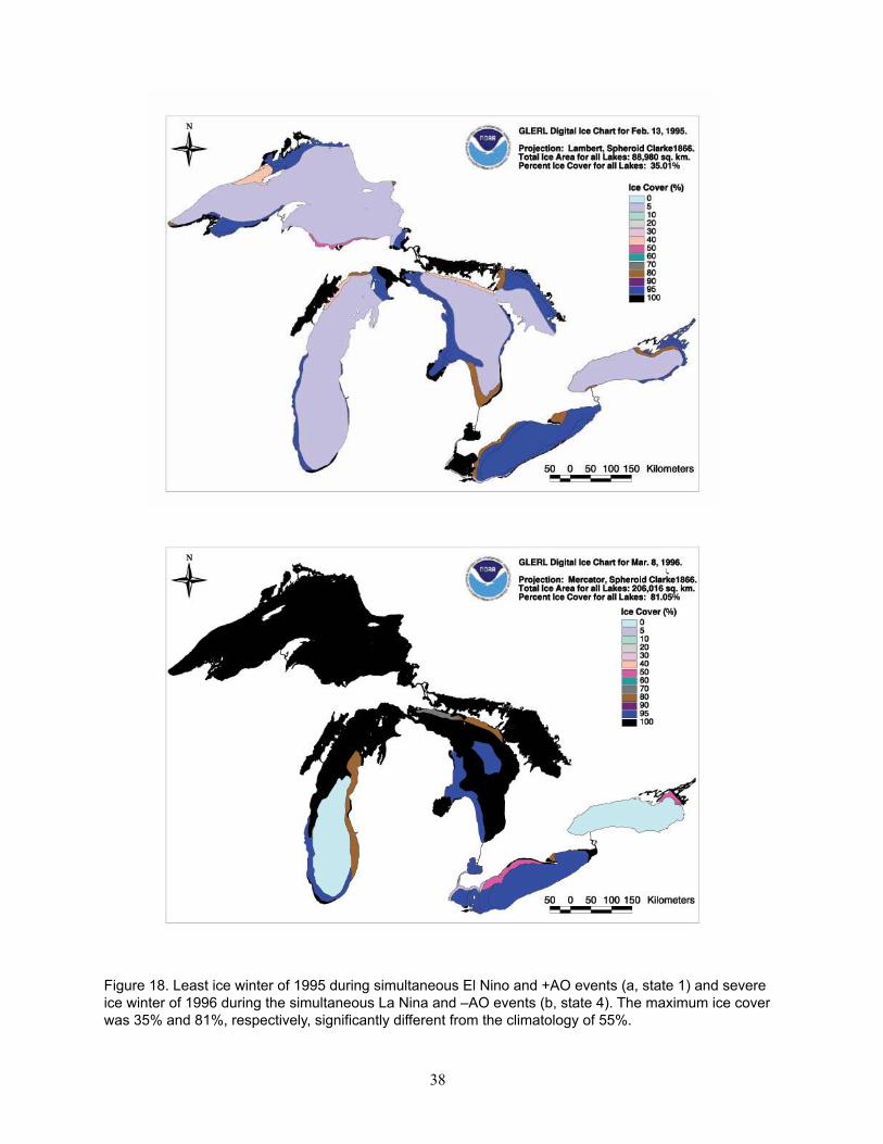
To demonstrate the combined effects of ENSO and AO, we chose climate states 1 and 4 because lake ice during these two states has proven predictable. Figure 18 only shows the spatial distribution of 1995 (state 1) and 1996 (state 4). During the simultaneous occurrence of El Niño and +AO in the 1995 winter, lake ice maximum extent was only 35.1% (Fig. 18a). During the simultaneous occurrence of La Niña and –AO (state 4), the lake ice maximum extent was 81% (Fig. 18b). It is clear that the combined effect of AO and ENSO possesses a greater predictability skill for long-term lake ice variability than individual indexes.

38

Figure 18. Least ice winter of 1995 during simultaneous El Nino and +AO events (a, state 1) and severe ice winter of 1996 during the simultaneous La Nina and –AO events (b, state 4). The maximum ice cover was 35% and 81%, respectively, significantly different from the climatology of 55%.

39

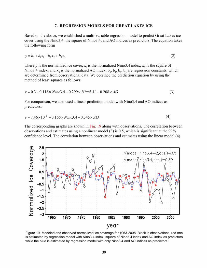
7. REGRESSION MODELS FOR GREAT LAKES ICE

Based on the above, we established a multi-variable regression model to predict Great Lakes ice cover using the Nino3.4, the square of Nino3.4, and AO indices as predictors. The equation takes the following form

€

y = b0 + b1x1 + b2x2 + b3x3 (2)

where y is the normalized ice cover, x1 is the normalized Nino3.4 index, x2 is the square of Nino3.4 index, and x3 is the normalized AO index; b0, b1, b2, b3 are regression constants, which are determined from observational data. We obtained the prediction equation by using the method of least squares as follows:

  (3)

For comparison, we also used a linear prediction model with Nino3.4 and AO indices as predictors:

(4)

The corresponding graphs are shown in Fig. 19 along with observations. The correlation between observations and estimates using a nonlinear model (3) is 0.5, which is significant at the 99% confidence level. The correlation between observations and estimates using the linear model (4)

Figure 19. Modeled and observed normalized ice coverage for 1963-2008. Black is observations, red one is estimated by regression model with Nino3.4 index, square of Nino3.4 index and AO index as predictors while the blue is estimated by regression model with only Nino3.4 and AO indices as predictors.

40

is 0.39, also significant at the 90% confidence level. This suggests that using the square of the Nino3.4 index (nonlinear model) instead of the Nino3.4 index itself (linear model) significantly improves the prediction of Great Lakes ice cover.

8. SUMMARY AND CONCLUSIONS

The impacts of ENSO and AO on Great Lakes ice cover were investigated using lake ice observations for winters 1963-2008 and NCEP reanalysis data. It was found that both ENSO and AO have impacts on Great Lakes ice cover, but neither dominates.

The relationship between ENSO and Great Lakes ice cover is asymmetric between the El Niño and La Niña events, behaving in a non-linear manner. During El Niño events, the Great Lakes SAT tend to be warmer-than-normal and have less ice cover. Strong El Niño events are often associated with least ice cover, which explained 53% of the least ice cover events during 1963-2008. Nevertheless, the impacts of La Niña events on Great Lakes ice cover are insignificant. Severe ice cover winters cannot be explained by La Niña events alone.

The Great Lakes regional climate including ice cover was also significantly influenced by AO. The impacts of AO on the Great Lakes tend to be linear, compared to ENSO. The Great Lakes SAT tend to be warmer-than-normal during a positive phase of AO and colder-than-normal during a negative phase of AO. From 1963 to 2008, almost all severe ice cover events occurred during a negative AO, and 5 of 13 least ice cover winters were during a positive phase of AO. Since both ENSO and AO have competing impacts on the Great Lakes area, the interference of these two forcing factors in this region is inevitable. When a winter occurs during an El Niño event and a positive phase of AO (state 1), the combined effects lead to a mild winter and less ice cover. When a winter occurs during a La Niña event and a negative phase of AO (state 4), the combined effects lead to a severe winter and more ice cover. During 1963-2008, there were five winters in state 1 (El Niño/+AO) and also five winters in state 4 (La Niña /-AO). These two states reinforce the linearity of the impacts of ENSO and AO. When a winter occurs during an El Niño event and a negative phase of AO (state 2), ice conditions on the Great Lakes depend on the strength of these two forcings. The observations suggest that when the El Niño event is strong, its warming influence can extend to the Great Lakes region and exceed the -AO cooling effect, leading to a mild winter and less ice cover. When an El Niño event is week, its warming effect cannot compete with the -AO cooling effect, leading to a severe winter and more ice cover. When a winter occurs during a La Niña event and a positive phase of AO (state 3), since the impacts of La Niña events on the Great Lakes are insignificant (although slightly warm SAT anomaly due to the northward advection of the Gulf of Mexico warm, moist air), the Great Lakes are dominated by a positive AO, leading to a mild winter and less ice cover. These two states reinforce the asymmetric response of the Great Lakes regional climate to ENSO.

41

The nonlinear effects of ENSO on Great Lakes ice cover are important in addition to AO effects. Although the correlation between the Nino3.4 index and ice coverage is insignificant (-0.18), the correlation coefficient between the square of Nino3.4 index and ice coverage (-0.45) turns out to be significant at the 99% confidence level. Based on the finding derived from data analysis, a multiple-variable nonlinear regression model was developed to predict lake ice cover using the Nino3.4 index, the square of Nino3.4 index and the AO index as predictors. Using the square of the Nino3.4 index (nonlinear model) instead of the index itself (linear model) can significantly improve the prediction skills of Great Lakes Ice cover.

9. ACKNOWLEDGEMENTS

We acknowledge support from the National Research Council for X. Bai and from the Great Lakes Restoration Initiative (GLRI) from EPA/NOAA. NCEP reanalysis data was provided by the NOAA/OAR/ESRL PSD, Boulder, Colorado, from http://www.cdc.noaa.gov/. The Nino3.4 index and AO index was provided by NOAA/CPC, from http://www.cpc.noaa.gov/products/precip/CWlink/.

10. REFERENCES

Assel, R.A. The 1997 ENSO Event and Implications for North American Laurentian Great Lakes Winter Severity and Ice Cover. Geophysical Research Letters 25(7):1031-1033 (1998).

Assel, R.A. and F.H. Quinn. A historical perspective of the 1976–77 Lake Michigan ice cover. Monthly Weather Review 107:336–341 (1979).

Assel, R.A. and D.M. Robertson. Changes in winter air temperatures near Lake Michigan during 1851–1993, as determined from regional lake-ice records. Limnology and Oceanography 40:165–176 (1995).

Assel, R.A., and S. Rodionov. Atmospheric teleconnections for annual maximal ice cover on the Laurentian Great Lakes. International Journal of Climatology 18:425–442 (1998).

Assel, R.A., C.R. Snider, and R. Lawrence. Comparison of 1983 Great Lakes winter weather and ice conditions with previous years. Monthly Weather Review 113:291–303 (1985).

Assel, R.A., K. Cronk, and D.C. Norton. Recent trends in Laurentian Great Lakes ice cover. Climatic Change 57:185-204 (2003).

Assel, R.A., S. Drobrot, and T. Croley. Improving 30-day Great Lakes Ice Cover Outlooks. Journal of Hydrometeorology 5:13-717 (2004a).

Assel, R.A., F.H. Quinn, and C.E. Sellinger. Hydro-climatic factors of the recent drop in Laurentian Great Lakes water levels. Bulletin of the American Meteorological Society 85:1143-1151 (2004b).

Barnston, A.G. Linear statistical short-term climate predictive skill in the Northern Hemisphere. Journal of Climate 7:1513–1564 (1994).

42

Barnston, A.G., R.E. Livezey, and M.S. Halpert. Modulation of Southern Oscillation Northern Hemisphere Mid-Winter Climate Relationships by the QBO. Journal of Climate 2:203-217 (1991).

Brown, R., W. Taylor and R.A. Assel. Factors affecting the recruitment of lake whitefish in two areas of northern Lake Michigan. Journal of Great Lakes Research 19:418–428 (1993).

Derome, J., and Coauthors. Seasonal predictions based on two dynamical models. Atmosphere–Ocean 39:485–501 (2001).

Gershunov, A., and T.P. Barnett. ENSO influence on intraseasonal extreme rainfall and temperature frequencies in the contiguous United States: observations and model results. Journal of Climate 11:1575–1586 (1998).

Halpert, M.S., and C.F. Ropelewski. Surface temperature patterns associated with the Southern Oscillation. Journal of Climate 5:577–593 (1992).

Hanson, P.H., C.S. Hanson, and B.H. Yoo. Recent Great Lakes ice trends. Bulletin of the American Meteorological Society 73:577–584 (1992).

Hodges, G. The new cold war. Stalking arctic climate change by submarine. National Geographic March:30–41 (2000).

Hoerling, M.P., A. Kumar, and M. Zhong. El Niño, La Niña and the nonlinearity of their teleconnections. Journal of Climate 10:1769–1786 (1997).

Hoerling M.P., A. Kumar, and T. Xu. Robustness of the nonlinear climate response to ENSO’s extreme phases. Journal of Climate 14:1277–1293 (2001).

Horel, J.D., and J.M. Wallace. Planetary-scale atmospheric phenomena associated with the Southern Oscillation. Monthly Weather Review 109:813–829 (1981).

Hoskins, B., and D. Karoly. The steady linear response of a spherical atmosphere to thermal and orographic forcing. Journal of Atmospheric Science 38:1179–1196 (1981).

Hurrell, J.W. Influence of variations in extratropical wintertime teleconnections on Northern Hemisphere temperature. Geophysical Research Letters 23:665–668 (1996).

Hurrell, J.W., and H. van Loon. Decadal variations in climate associated with the North Atlantic Oscillation. Climate Change 36:301–326 (1997).

Kalnay and Coauthors. The NCEP/NCAR 40-year reanalysis project. Bulletin of the American Meteorological Society 77:437-470 (1996).

Kiladis G.N., and H.F. Diaz. Global climatic anomalies associated with extremes in the Southern Oscillation. Journal of Climate 2:1069–1090 (1989).

Livezey, R.E., A. Leetmaa, M. Mautani, H. Rui, M. Ji, and A. Kumar. Teleconnective response of the Pacific–North American region atmosphere to large central equatorial Pacific SST anomalies. Journal of Climate 10:1787–1820 (1997).

43

Magnuson, J., C. Bowser, R.A. Assel, B. DeStasio, J. Eaton, E. Fee, P. Dillon, L. Mortsch, N. Routlet, R. Quinn, and D. Schindler. Region 1-Laurentian Great Lakes and Precambrian Shield, in Symposium Report, Regional Assessment of Freshwater Ecosystems and Climate Change in North America, American Society of Limnology and Oceanography, and North American Benthological Society (1995).

Mo, K.C., and R.E. Livezey. Tropical–extratropical geopotential height teleconnections during the Northern Hemisphere winter. Monthly Weather Review 114:2488–2414 (1986).

Niimi, A.J. Economic and environmental issues of the proposed extension of the winter navigation season and improvements on the Great Lakes-St. Lawrence Seaway system. Journal of Great Lakes Research 8:532–549 (1982).

Rodionov, S., and R.A. Assel. Atmospheric teleconnection patterns and severity of winters in the Laurentian Great Lakes basin. Atmosphere Oceans 38:601–635 (2000).

Rodionov, S., and R.A. Assel. Winter severity in the Great Lakes region: a tale of two oscillations. Climate Research 24:19-31 (2003).

Rodionov, S., R.A. Assel, and L.R. Herche. Tree-structured modeling of the relationship between Great Lakes ice cover and atmospheric circulation patterns. Journal of Great Lakes Research 4:486-502 (2001).

Ropelewski C.F., and M.S. Halpert. North American precipitation and temperature patterns associated with El Niño Southern Oscillation (ENSO). Monthly Weather Review 114:2352–2362 (1986).

Sellinger, C.E., C.A. Stow, E.C. Lamon, and S.S. Qian. Recent Water Level Declines in the Lake Michigan-Huron System. Environmental Science & Technology 42: 367-373 (2008).

Shabbar, A., and A.G. Barnston. Skill of seasonal forecasts in Canada using canonical correlation analysis. Monthly Weather Review 124:2370–2385 (1996).

Smith, J.B. The potential impacts of climate change on the Great Lakes. Bulletin of the American Meteorological Society 72:21–28 (1991).

Thompson D. W. J, and J. M. Wallace. The Arctic Oscillation signature in the wintertime geopotential height and temperature fields. Geophysical Research Letters 25:1297–1300 (1998).

Trenberth, K.E., G.W. Branstator, D. Karoly, A. Kumar, N.-C. Lau, and C. Ropelewski. Progress during TOGA in understanding and modeling global teleconnections associated with tropical sea surface temperatures. Journal of Geophysical Research 103:14 291–14 324 (1998).

Vanderploeg, H.A., S.J. Bolsenga, G.L. Fahnenstiel, J.R. Liebig, and W.S. Gardner. Plankton ecology in an ice-covered bay of Lake Michigan: utilization of a winter phytoplankton bloom by reproducing copepods. Hydrobiologia 175–183 (1992).

Wallace, J.M., and D. Gutzler. Teleconnection in the geopotential height field during the Northern Hemisphere winter. Monthly Weather Review 109:784–812 (1981).

44

Wang, J., and M. Ikeda. Arctic Oscillation and Arctic Sea-Ice Oscillation. Geophysical Research Letters 27:1287-1290 (2000).

Wang, J., J. Zhang, E. Watanabe, K. Mizobata, M. Ikeda, J.E. Walsh, X. Bai, and B. Wu. Is the Dipole Anomaly a major driver to record lows in the Arctic sea ice extent? Geophysical Research Letters 36:L05706, doi:10.1029/2008GL036706 (2009).

Wang, J., X. Bai, G. Leshkevich, M. Colton, A. Clites, and B. Lofgren, 2010. Severe ice cover over the Great Lakes during winter 2008-2009, AGU EOS, February 2. 91 (5): 41-42 (2010).

Wu, A., W.W. Hsieh, and A. Shabbar. The nonlinear patterns of North American winter temperature and precipitation associated with ENSO. Journal of Climate 18:1736–1752 (2005).

Wu, A., W.W. Hsieh, and A. Shabbar. The nonlinear association between the Arctic Oscillation and North American winter climate. Climate Dynamics 26:865-879 (2006).

Zwiers, F. A potential predictability study conducted with an atmospheric general circulation model. Monthly Weather Review 115:2957–2974 (1987).