DPRIETI Discussion Paper Series 15-E-051

No Lending Relationships and Liquidity Management ofSmall Businesses during a Financial Shock

TSURUTA DaisukeNihon University

The Research Institute of Economy, Trade and Industryhttp://www.rieti.go.jp/en/

RIETI Discussion Paper Series 15-E-051

April 2015

No Lending Relationships and Liquidity Management of Small Businesses during a Financial Shock*

TSURUTA Daisuke

College of Economics, Nihon University

Abstract

We investigate the determinants of the end of lending relationships with banks using small business

data. We also investigate how small businesses without lending relationships financed credit demand

during the global financial shock. First, we find that firms with high internal cash holdings, lower

growth, and low working capital were more likely to end lending relationships with banks.

Supply-side effects on the determinants of the end of relationships are insignificant. Second, when

firms experienced credit demand during the financial shock, those with lending relationships

increased bank borrowings while those without lending relationships reduced internal cash. However,

if we examine cash-rich firms, both firms with and without relationships reduced cash holdings to

finance working capital during the shock period. Third, firm performance (in terms of profitability)

was neither lower nor higher for firms that did not have lending relationships with banks during the

shock period.

Keywords: Lending relationship, Small business, Financial shock

JEL classification: G21; G32

RIETI Discussion Papers Series aims at widely disseminating research results in the form of professional

papers, thereby stimulating lively discussion. The views expressed in the papers are solely those of the

author(s), and neither represent those of the organization to which the author(s) belong(s) nor the Research

Institute of Economy, Trade and Industry.

*This study was conducted as part of the Project ''Study on Corporate Finance and Firm Dynamics'' at the Research Institute of Economy, Trade and Industry (RIETI). This study uses microdata from the Surveys for the Financial Statements Statistics of Corporations by Industry (Houjin Kigyou Toukei Chosa) conducted by the Ministry of Finance and the Basic Survey of Small and Medium Enterprises (Chusho Kigyou Jittai Kihon Chosa) conducted by the Small and Medium Enterprise Agency. The study was supported by a Grant-in-Aid for Young Scientists (B) from the Japan Society for the Promotion of Science. The author would also like to thank Hikaru Fukanuma, Kaoru Hosono, Daisuke Miyakawa, Yoshiaki Ogura, Arito Ono, Hirofumi Uchida, Iichiro Uesugi, Hajime Tomura, Wako Watanabe, Peng Xu, and Yukihiro Yasuda for many valuable comments. The seminar participants at RIETI also provided useful comments. All remaining errors are mine.

1 Introduction

We investigate whether having no lending relationships was costly for small businesses

during the financial shock in 2008. As many studies (for example, Petersen and Rajan,

1994; Berger and Udell, 1995) argue, lending relationships with banks are valuable for

small businesses. As Petersen and Rajan (1994) argue, long-term lending relationships

with banks enhance the credit availability of small businesses because the relationships

mitigate the information asymmetry between banks and small businesses. During the fi-

nancial shock, these relationships played important roles for small businesses. As previous

studies (for example, Berlin and Mester, 1999; Boot, 2000) argue, through intertemporal

smoothing of loan interest rates, banks were able to offer credit during the financial shock.

This is another benefit of lending relationships for small businesses.

Previous empirical studies of relationship banking (for example, Jiangli et al., 2008;

Cotugno et al., 2013; Dewally and Shao, 2014; Gobbi and Sette, 2014) show that firms with

strong relationships with banks can use bank loans during times of economic distress. For

example, using Italian data, Cotugno et al. (2013) show that a strong lender–borrower

relationship mitigates credit rationing for borrowing firms (including small businesses)

during a credit crunch period. If small businesses with long-term relationships do not

face credit constraints during financial shocks, they increase bank loans to finance their

liquidity shortages. In contrast, small businesses without lending relationships face severe

credit constraints if they face large and unexpected financial shocks.1

Using listed firm data, some studies (for example, Slovin et al., 1993; Yamori and

Murakami, 1999; Sohn, 2010) show the negative effects of ending a relationship with a

bankrupt bank for client firm performance. In addition, using Norwegian listed firm

1Recent studies about liquidity management argue that firms (especially large firms) use credit lineswhen they face liquidity shortages or financial shocks. Focusing on the recent financial crisis, Campelloet al. (2011, 2012) show that larger-sized firms drew more funds from their credit lines during the crisis ifthey are relatively small, noninvestment grade, and unprofitable. Campello et al. (2012) define a “smallfirm” as one with sales revenue of less than $1 billion. Therefore, these small firms, as defined in Campelloet al. (2012), are not small businesses. Small businesses, which have unstable cash flows and are morelikely to suffer from low cash flows, cannot use credit lines.

2

data, Ongena and Smith (2001) investigate the determinants of the duration of bank

relationships. Focusing on zero leverage, Strebulaev and Yang (2013) show that listed

firms have zero debts when they have high cash holdings and are more profitable. However,

to our knowledge, only a few papers (for example, Cole, 2010) investigate whether the

cost of not having a lending relationship with any bank is significant for small businesses.2

Furthermore, whether the negative effects of having no lending relationships are significant

for small businesses during the financial shock is not clear from previous studies.

To address this issue, we first investigate what determined the decisions of small busi-

nesses to end lending relationships during the preshock period. As large amounts of

precautionary cash holdings decrease the demand for bank loans, small businesses with

large amounts of internal cash are more likely to end relationships with banks. Further-

more, firms with few investment opportunities only need small loans, so they are more

likely to end their bank relationships. On the other hand, if credit supply determines the

ending of bank relationships, small businesses end their relationships unless their credit

demand is high. Second, we investigate the effects of the ending of bank relationships

during the unexpected global financial crisis. If credit constraints for small businesses

without lending relationships are severe, small businesses do not borrow sufficient funds

from banks when they have credit demand. In addition, they have to borrow from ex-

pensive financing sources, which is a cost of having no lending relationships. Third, we

investigate the effects of having no lending relationships on firm performance during the

shock period. If banks do not offer sufficient funds for those without relationships, their

firm performance (in terms of profitability) is lower.

We examine the above hypothesis using firm-level data of Japan for the 2000s. Japanese

data are suitable for investigating the effects of ending lending relationships with banks.

First, as Hoshi et al. (1991) argue, main bank relationships mitigate the effects of credit

2In addition, previous studies investigate the negative effects of firms exogenously ending lendingrelationships with a particular bank. Our study investigates the negative effects of an exogenous shockin which borrowers endogenously end lending relationships with all banks before the shock period.

3

rationing in Japan. Therefore, many studies argue that lending relationships are valuable

for small businesses. Second, as Miwa (2012) argues, Japanese firms (including small

businesses) are reducing their borrowings and the ratio of firms with no borrowings is

increasing. Therefore, our Japanese dataset provides data on firms without lending rela-

tionships. For most small businesses, the shock was an unexpected event, so they could

not decide to end their relationships while taking the shock into account. Therefore, the

selection bias is not serious enough to prevent our investigation of the cost of having no

relationships during the shock period. Third, as Uchino (2013) shows, although bond mar-

kets were seriously damaged by the global financial crisis, the banking market in Japan

did not shrink. In addition, the real growth rates of GDP dropped from 1.8% in fiscal

year (FY) 2007 to –3.7% in FY2008 and –2.0% in FY2009, implying that the real shock

was serious for small businesses. This implies that the benefits of lending relationships

existed in Japan during the shock period.

The main findings of this paper are as follows. First, small businesses with higher cash

holdings and cash flow to total assets ratio are more likely to end lending relationships with

banks. This implies that cash holdings are a substitute for bank loans. Furthermore, they

are likely to end lending relationships when their asset growth rate is lower. This implies

that they end relationships because they have less profitable investment opportunities.

The ending of relationships caused by denied loan applications is not observed, implying

that the supply effects on the ending of relationships are insignificant.

Second, following the global financial shock in 2008, small businesses without lending

relationships increased their bank loans to finance credit demand, but by a smaller amount

than small businesses with relationships. However, the interest rates for small businesses

without relationships are not higher than those for small businesses with relationships,

suggesting that they use expensive sources of financing. This implies that small businesses

did not face severe financial constraints during the financial crisis if they did not have

lending relationships. In addition, if we match the firms with relationships and those

4

without using the propensity score matching method, the differences are not statistically

significant, implying that firms with lending relationships increased their bank borrowings

by less if they had sufficient internal cash.

Third, the performance of firms without relationships (in terms of profitability) was

neither lower nor higher than for firms with relationships during the shock period. This

result also implies that credit constraints for firms without relationships were not severe.

The remainder of the paper is organized as follows. Section 2 describes the dataset

and the hypotheses to be tested. We identify the determinants of the ending of lending

relationships in Section 3. In Section 4, we present the estimated results for the effects of

having no lending relationships during the shock period. Section 5 concludes the paper.

2 Data and Hypothesis

2.1 Data

We use annual firm-level data of Surveys for the Financial Statements Statistics of Corpo-

rations by Industry (hereafter FSSC; Houjin Kigyou Toukei Chosa in Japanese) conducted

by the Ministry of Finance. According to the website of the Ministry of Finance,3 the

FSSC are “one part of the fundamental statistical surveys under the Statistics Act and

have been conducted as sampling surveys so as to ascertain the current status of business

activities of commercial corporations in Japan.” The target firms of the FSSC are all

commercial corporations in Japan. All firms with capital of 1 billion yen or more are

included. Those with capital of between 100 million and 600 million yen are randomly

selected with equal probability. Those with less than 100 million yen of capital are ran-

domly sampled every fiscal year. Therefore, of the firms with less than 100 million yen in

capital, a different sample of target firms is selected each fiscal year. The response rates

for each fiscal year are around 80%. The FSSC covers a large number of small businesses,

3For details of the survey see: http://www.mof.go.jp/english/pri/reference/ssc/index.htm.

5

including firms with lending relationships and those with no relationships, implying that

these data include various types of firms. The FSSC include data of firms’ balance sheets

and profit and loss statements. Data of firms’ balance sheets are available at the begin-

ning and end of each fiscal year. The data at the end of fiscal year t are set equal to the

data at the beginning of fiscal year t+1. In this paper, we limit our analysis to “small

and medium enterprises” (SMEs) as defined in the Small and Medium-sized Enterprise

Basic Law.4 Under this definition, our sample data include firms with a large number of

employees and capital stock, so we omit firms with 500 or more employees and those with

a capital stock of 500 million yen or more. The number of firm-year observations is 68,325

during the preshock period of 2001–2007. The number of firm-year observations during

the shock period of 2008 is 9,788. Table 1 shows the number of observations divided by

firm size. As this table shows, our data cover both smaller and larger small businesses.

2.2 Descriptive Statistics

Before the econometric analysis, we describe our data on small businesses’ bank bor-

rowings in the 2000s in Japan. Table 2 shows the quartiles of total bank borrowings

normalized by total assets. The median of total bank borrowings decreased during the

2000s, from 24.30% (in FY2001) to 12.88% (in FY2008). Similarly, the third quartiles

decreased. In particular, the first quartiles of total bank borrowings are 0.00% after 2001,

suggesting that more than 25% of small businesses did not have lending relationships with

any banks.5

4According to the 2005 White Paper on Small and Medium Enterprises in Japan, “small and mediumenterprises” under the Small and Medium-sized Enterprise Basic Law are defined as “enterprises withcapital stock of not in excess of U300 million or with 300 or fewer regular employees, and sole proprietor-ships with 300 or fewer employees. However, SMEs in the wholesale industry are defined as enterpriseswith capital stock not in excess of U100 million or with 100 or fewer employees; SMEs in the retailindustry are defined as enterprises with capital stock not in excess of U50 million or with 50 or feweremployees; and SMEs in the service industry are defined as enterprises with capital stock not in excessof U50 million or with 100 or fewer employees. “Small enterprises” are defined as enterprises with 20 orfewer employees. In the commercial and service industries, however, they are defined as enterprises withfive or fewer employees.

5These results are consistent with those in Miwa (2012).

6

Table 3 shows the median of total bank borrowings using subsamples by firm size.6

This table shows that all four groups of firms decreased their bank borrowings. Fur-

thermore, the bank borrowings for very small firms (firms with 20 employees or fewer)

and large firms (firms with 301 employees or more) were lower. Table 4 shows the ratio

of firms without lending relationships, divided by firm size. This table shows that the

ratios of firms without lending relationships increased during the sample period in all

four groups. Furthermore, the ratio for the smallest-sized firms is the largest. Intuitively,

very small firms depend on bank borrowings because they are informationally opaque and

cannot borrow without relationship lenders. However, the results are inconsistent with

this intuition. Figure 1 shows the kernel function of total bank borrowings having divided

the sample by fiscal year. This figure also shows that the number of zero-lending firms

is increasing by fiscal year. The peak of the function is less than 0.05 and the density of

the peak is also increasing by fiscal year. This implies that many small businesses had no

bank borrowings before the financial shock in 2008.

2.3 Hypothesis

2.3.1 Determinants of Ending Relationships with Banks

The one reason for small businesses continuing the lending relationships with banks is

that they have credit needs to finance investment opportunities. Low investment oppor-

tunities lead to a low opportunity cost of holding cash, which causes low credit demand

of bank loans and the end of lending relationships. We predict that firms with low invest-

ment opportunities are likely to end the relationships. As our data consisted mainly of

information about small businesses, Tobin’s q is unavailable. Instead, we use firm growth

as a proxy for investment opportunities.

Additionally, internal cash can substitute for continuing lending relationships with

6We divide the sample into four groups: firms with 20 employees or fewer, firms with 21 to 100employees, firms with 101 to 300 employees, and firms with 301 employees or more.

7

banks. According to Bates et al. (2009), one of the main reasons that firms accumulate

cash holdings is because of a precautionary motive. In general, small businesses cannot

use credit lines for financing sudden credit needs. Thus, they accumulate more cash in sit-

uations when they need to cope with adverse shock because they face credit constraint. If

credit-constrained small businesses anticipate that they cannot borrow a sufficient amount

from banks during adverse shock, they accumulate larger amounts of cash holdings. This

leads to low demand for bank loans and the ending of lending relationships with banks.

In addition, firms with high cash flows do not need to borrow from banks, and thus they

are likely to end their lending relationships.

Furthermore, other sources of finance can substitute for bank loans. Some firms borrow

funds from nonfinancial firms. If they can borrow sufficient funds from them, they are

likely to end their lending relationships with banks. Lastly, firms with high working

capital requirements have larger credit demands, so they are not likely to end their lending

relationships.

In sum, we predict the following hypothesis: firm growth, cash holdings, cash flows,

and lending relationships with nonfinancial firms have positive effects on ending relation-

ships with banks. Furthermore, working capital requirements have negative effects on

ending relationships with banks.

2.3.2 Effects of the Global Shock

During the financial crisis, many firms faced financial shortages (for example, temporary

liquidity shortfalls and increasing working capital requirements). The shock was severe

and unexpected, and firms reduced their financial shortfalls by increasing bank loans.

Therefore, they increased the demand for borrowings to cope with the negative effects of

the shock. Firms with lending relationships can increase their borrowings from banks if the

banks can provide liquidity by intertemporal smoothing of loan rates (Berlin and Mester,

1999). In contrast, firms with no lending relationships can face severe financial constraints.

8

Under the severe credit constraints of small businesses without lending relationships,

these firms must use expensive financing sources, implying they pay higher interest rates.

Furthermore, they face underinvestment problems, which lower their performance.

On the other hand, if firms without lending relationships have sufficient cash holdings

to cope with shocks, the credit constraint is not severe for them even though they have

lending relationships with banks. If this is true, they do not use expensive financing

sources and experience lower performance.

3 End of Lending Relationships

3.1 Estimation Strategy

In this subsection, we investigate the relationships between cash holdings and end of

lending relationships with banks. We estimate the following equation:

End∗i,t = α1Cash Holdingsi,t + α2Cash F lowi,t + α3Firm Sizei,t (1)

+ α4Firm Growthi,t + α5Nonbanking Relationships

+ α6WCRi,t + α7Endi,t−1 + ϵi + ζt + ηi,t

Endi,t = 1 if End∗i,t > 0

Endi,t = 0 otherwise,

where ηi,t is the error term of firm i in year t, ζt is the year fixed effect from 2001 to 2007,

and ϵi is the industry fixed effect.

The dummy variable Endi,t takes a value of one if short-term and long-term borrow-

ings from financial institutions at the end of fiscal year t are zero, and zero otherwise.

As there are only a small number of instances of data for two or more consecutive fiscal

years, we define ending relationships using data for one fiscal year.7 End∗i,t is a latent

7If we use short-term borrowings to define Endi,t, the estimation results are similar to those described

9

variable indicating the end of lending relationships, which is the net benefit from end-

ing the relationships. If End∗i,t is greater than zero, firms and banks end their lending

relationships.

Independent variables are End at the beginning of the fiscal year, cash holdings, cash

flows, firm size, firm growth, nonbanking relationships dummy, tangible fixed assets, and

working capital requirements (hereafter, WCR). We also control year and industrial fixed

effects using year and industrial dummies. Cash holdings are defined as the ratio of a

firm’s cash holdings to total assets at the beginning of each fiscal year. Cash flows are

defined as firm earnings before interest, taxes, depreciation, and amortization (hereafter,

EBITDA), normalized by total assets in fiscal year t. We predict that cash holdings and

flows have positive effects on the end of relationships. Firm size is defined as the natural

logarithm of a firm’s total assets at the beginning of the fiscal year. Firm growth is defined

as the natural logarithm of a firm’s total assets at the end of the fiscal year minus those at

the beginning of the fiscal year. If growing firms need to finance investment opportunities

using bank loans, the coefficients of firm growth are negative.

Nonbanking relationships is a proxy variable for lending relationships with nonfinancial

firms, which equals one if a firm’s total borrowings from nonfinancial firms are nonzero,

and zero otherwise. If lending relationships with nonfinancial firms are substitutes for

relationships with banks, nonbank relationships have positive effects on the end dummy.

In contrast, the relationships with nonfinancial firms complement those with banks, and

thus the dummy has negative effects. Tangible fixed assets are defined as the ratio of a

firm’s tangible fixed assets to total assets. We predict that firms with high tangible fixed

assets have long-term debts, so they are not likely to end their bank relationships. WCR

is defined as the sum of trade receivables and inventories, minus trade payables (Hill et al.,

2010), which is a proxy for credit demand. Firms with higher WCR require short-term

credit, so they are not likely to end their lending relationships with banks.

in this paper.

10

3.2 Estimation Results

Table 5 shows summary statistics for the variables in equation (1). Table 6 shows the

estimation result for equation (1). We show the results using all observations in column

(1), those using small firms in column (2), and those using medium firms in column (3).

Small firms are defined as firms with 20 or fewer employees, and medium firms are defined

as firms with 21 or more employees. The marginal effects of each variable at the mean

are provided in each column.

The coefficients of cash holdings and cash flows are positive and statistically significant

at the 1% level (column 1). The effect of cash holdings for medium firms is insignificant,

but that for small firms is still positive and statistically significant. Furthermore, the

effects of cash flows are positive and statistically significant for both small and medium

firms (columns 2 and 3). These results suggest that cash-rich firms are likely to end

relationships with banks. The marginal effect of cash flow is 0.4144, which means a one

standard deviation increase in cash flow raises the probability of ending relationships by

3.41%. The effects of firm size are negative and statistically significant apart from in

column (3).

The coefficients of firm growth are all negative and statistically significant at the

1% level. These results suggest that firms end lending relationships with banks because

they do not have enough investment opportunities. The marginal effect of firm growth

is –0.2211, which means that a one standard deviation increase in sales growth reduces

the probability of ending relationships by 4.42%. This suggests that the magnitude of

sales growth is larger than those of cash flow and working capital. The coefficients of

nonbanking relationships are all negative and statistically significant (not positive), sug-

gesting that firms having relationships with nonfinancial firms are not likely to end their

relationships with banks. This implies that the lending relationships with nonfinancial

firms complement those with banks. As we predicted, the coefficients of tangible assets

are all negative and statistically significant. The coefficients of WCR are all positive and

11

significant, which is also consistent with our prediction. Demand for short-term credit is

high in firms with high WCR, so they are not likely to end their relationships with banks.

A one standard deviation increase in working capital reduces the probability of ending

relationships by 2.24%.

In columns (4)–(6), we only use observations whose lagged values equal zero, which are

observations having relationships with banks in the previous year. The coefficient of cash

flows for small firms changes to be statistically insignificant (column 5). Additionally, the

coefficients of firm size are all statistically significant. The results for the other coefficients

of the independent variables are similar to those in columns (1)–(3), suggesting that the

results are robust.

In sum, the estimation results for ending relationships imply the following. First, firms

with high liquidity are likely to end lending relationships. Second, firms are likely to end

relationships because they have no demand for bank credit (for example, low growth, low

working capital requirements, low tangible assets).8

3.3 Supply-Side Effects

From the results using FSSC, we cannot determine whether supply-side effects include

the ending of relationships. We can conclude that because banks reject loan applications

from small business borrowers, small businesses are forced to end their relationships with

banks. To investigate the supply-side effects on the ending of relationships, we match

the FSSC data to the aggregate diffusion index of financial institution lending attitudes

(hereafter, “financial DI”) from the Bank of Japan’s TANKAN survey (Short-term Eco-

nomic Survey of Enterprises). The TANKAN survey questions firms about their business

conditions, including one question that addresses the lending attitude of financial insti-

tutions. Financial DI equals “accommodative” minus “severe” measured in percentage

points and relates to the present lending attitude of financial institutions. A small value

8The main results are similar if we divide the sample by major industries.

12

of financial DI means that lending attitudes are severe. As financial DI is available at the

industry level, we match financial DI using firm industry codes. The TANKAN survey is

seasonal data, so the data are averaged for each fiscal year.

We estimate equation (1) using financial DI as an additional independent variable.

Industry dummies are omitted because financial DI is measured at the industry level.

Table 7 shows the estimation results. If we use all observations, the coefficient of financial

DI is negative and statistically significant at the 10% level (column 1). This result suggests

that firms end relationships when the lending attitude of banks is severe, implying that the

supply-side effects on ending relationships are significant. However, if we split the sample

by firm size, or limit our analysis to observations that have not ended relationships by the

beginning of the fiscal year, the coefficients of financial DI are not statistically significant

(columns 2–6). These results suggest that the supply-side effects are not robust.

Additionally, we use the “Basic Survey of Small and Medium Enterprises” in FY2004,

conducted by the Small and Medium Enterprise Agency.9 This survey targets firms de-

fined as small and medium enterprises under the Small and Medium Enterprise Basic

Law. Target firms are selected from the Establishment and Enterprise Census of Japan,

conducted by the Ministry of Internal Affairs and Communications. The survey ques-

tionnaires were sent to around 110,000 selected firms. One of the questions relates to

the status of loan applications to main banks: “Regarding your loan applications to your

main bank during the past year, which of the following is most accurate?”.

Respondents were asked to select one of the following six responses: 1) Applications re-

jected or amounts requested reduced, 2) Could borrow amounts requested without changes

to borrowing terms, 3) Borrowing terms severe, but could borrow amounts requested, 4)

Could borrow amounts requested after easing of borrowing terms, 5) Bank suggested

increasing loan amount, and 6) Have not submitted loan applications.10

9See the website of the Small and Medium Enterprise Agency for a detailed explanation about thissurvey: http://www.chusho.meti.go.jp/koukai/chousa/kihon/index.htm (in Japanese).

10For the distributions of each answer, see Figure 2-3-14 in Agency (2007):http://www.chusho.meti.go.jp/pamflet/hakusyo/h19/download/2007hakusho eng.pdf.

13

Table 8 shows the survey results for each response, in terms of both absolute number

and percentage of total responses, after dividing the sample by whether relationships

had ended or not. If the supply-side effects on ending relationships are significant, the

percentage of firms selecting “Applications rejected or amounts requested reduced” would

be high in the group of firms ending relationships. However, the percentage of firms

selecting this response is 0.37%, or only four firms. This suggests that the ending of

relationships because of banks denying applications of loans is rare. On the other hand,

the percentage of firms selecting “Have not submitted loan applications” is 99.54% in

the group of firms with no borrowings, suggesting that firms do not borrow because they

do not need loans. These results indicate that the main causes of the end of lending

relationships are firm factors, not supply-side factors.

4 Financial Shock and Liquidity Management

4.1 Estimation Strategy

4.1.1 Financial Shock and Financing Sources

In the previous section, we showed that firms with large internal cash holdings, those

with lower growth opportunities, and those with lower credit demand are more likely to

end lending relationships. In this section, we examine the financing sources that small

businesses use for credit demand and when they face exogenous financial shocks.

If lending relationships are valuable for small businesses, those without lending re-

lationships would face severe financial constraints during a financial shock. If this is

true, they cannot borrow sufficient funds from banks when they have high credit de-

mand. Furthermore, they have to use expensive financing sources. Consequently, firms

without lending relationships experience lower firm performance because of severe credit

constraints. If financial constraints for firms without lending relationships are insignif-

icant, the firms can borrow from banks and do not suffer lower firm performance. As

14

we showed in the previous section, those without relationships have higher internal cash

holdings. If firms without lending relationships have sufficient internal cash, they reduce

cash holdings instead of increasing bank loans when they face a liquidity shock. Addi-

tionally, they do not face severe credit constraints, so they do not use expensive financing

sources. As a result, this also means that the firm performance of these firms is not lower.

To test the above hypotheses, we identify which firms needed to increase bank loans

during the shock period. We use WCR as a proxy of financial needs. As we argued, WCR

is defined as the sum of trade receivables and inventories, minus trade payables. Firms

need to finance their WCR using short-term financial debt or by reducing cash holdings

(Preve and Sarria-allende, 2010). During an (unexpected) recession period, the WCR

changes exogenously and is less controllable for firms for the following reasons. First, as

firms’ sales decrease unexpectedly in a recession period, the level of unsold inventories

increases. Second, because firms’ production costs should decline because of a reduction

in sales, the level of trade payables should decrease. During a recession period, the change

in trade payables is caused mainly by the reduction in the volume of real transactions

(Tsuruta and Uchida, 2013). These cause an increase in WCR, so firms need to finance

the short-term credit demand during the recession. For small businesses, the financing

sources are limited to indirect finance, so they should use bank loans for financing. On the

other hand, small businesses can reduce cash holdings if they accumulate precautionary

savings.

4.1.2 Bank Borrowings

To investigate the effects of WCR on bank loans during the shock period, we estimate the

following regression:

∆Bank Borrowingsi,t =∑end

∑shock

βend,shock1 ∆WCRend,shock

i,t

15

+ Xi,tβ2 + θi + ιt + κi,t, (2)

where κi,t is the error term of firm i in year t, ιt is year fixed effects from 2006 to 2008, and

θi is industry fixed effects. End equals one if firm i does not have lending relationships at

the beginning of fiscal year t, and zero otherwise. Shock equals one if t equals 2008, and

zero otherwise. Xi,t is a vector of control variables, which are firm scale at the beginning

of fiscal year t, firm growth in fiscal year t, end dummy at the beginning of fiscal year t,

cash flows in fiscal year t, collateral assets at the beginning of fiscal year t, leverage at

the beginning of fiscal year t, and interest rate in fiscal year t.

∆Bank Borrowingsi,t is the growth rate of a firm’s total bank borrowings {[(short-

term bank borrowings at the end of the fiscal year + long-term bank borrowings at the

end of the fiscal year) – (short-term bank borrowings at the beginning of the fiscal year

+ long-term bank borrowings at the beginning of the fiscal year)] / total assets at the

beginning of the fiscal year}. Firms generally use short-term borrowings to finance their

working capital. However, some firms use long-term borrowings, so we also include long-

term bank borrowings.11

The shock period is FY2008 and the preshock period is the fiscal year prior to 2007.

To compare before and during the shock period, we include two fiscal years (2006 and

2007) before the Lehman shock. The end of FY2008 is March 2009 and is thus after the

collapse of Lehman Brothers. To compare the effects of ending relationships before the

shock period, we use only the data for FY2008.

We use the annual growth rate of WCR (∆WCRi,t) between the beginning and the

end of the fiscal year, which is defined as [(WCR at the end of the fiscal year – WCR

at the beginning of the fiscal year) / total assets at the beginning of the fiscal year]. If

firms with larger financial shortages increase bank borrowings, the coefficient of ∆WCRi,t

is positive. To investigate the heterogeneous effects of ∆WCRi,t between firms with

11In FSSC, bank borrowings are borrowings from deposit-taking financial institutions, government-affiliated financial institutions, and nondeposit-taking financial institutions (finance company).

16

relationships and those without relationships during the shock and preshock periods, we

use four variables: ∆WCRend,shocki,t , where end (at the beginning of fiscal year t)=0,1 and

shock=0,1. ∆WCRend,shocki,t equals ∆WCRi,t if the end dummy at the beginning of the

fiscal year is j and shock equals k, zero otherwise, where j=0,1 and k=0,1.

If firms use bank loans when they face increasing credit demand, the coefficients

of ∆WCRi,t are positive. If lending relationships with banks are valuable for small

businesses, small businesses with lending relationships finance their increase in WCR

using bank loans. In contrast, small businesses without lending relationships do not

finance WCR using bank loans, so the effects of ∆WCRi,t are larger for small busi-

nesses with lending relationships. In addition, those effects are larger during an un-

expected financial shock. In sum, we predict that βend=0,shock=01 > βend=1,shock=0

1 and

βend=0,shock=11 > βend=1,shock=1

1 if lending relationships are valuable for small businesses.

Furthermore, βend=0,shock=01 < βend=0,shock=1

1 is supported if small businesses depend on

bank borrowings more during an unexpected financial shock.

The definitions of the control variables are as follows. We use the natural logarithm

of total assets at the beginning of the fiscal year as a proxy of firm scale. Firm growth is

defined as firm scale at the end of the fiscal year minus firm scale at the beginning of the

fiscal year. We use EBITDA as a proxy of cash flows. We use the ratio of a firm’s tangible

fixed assets to total assets at the beginning of the fiscal year as a proxy of collateral assets.

Leverage is the ratio of a firm’s book value of total debts to book value of total assets at

the beginning of the fiscal year. Interest rate is defined as the ratio of a firm’s interest

expenses in fiscal year t to the sum of its short- and long-term debt and discounted notes

receivable averaged between the beginning and end of fiscal year t.

4.1.3 Financial Cost

If firms without lending relationships face severe credit constraints during a financial

shock, they have to use high-cost financing, such as nonbank loans. To investigate whether

17

firms without lending relationships face severe constraints, we estimate the following re-

gression:

Interest Ratei,t =∑end

∑shock

γend,shock1 ∆WCRend,shock

i,t + Yi,tγ2 + λi + µt + νi,t, (3)

where interest rate is a dependent variable for firm i in fiscal year t; Yi,t is a vector of

control variables (firm scale at the beginning of fiscal year t, firm growth in fiscal year t,

cash flow in fiscal year t, collateral assets at the beginning of fiscal year t, leverage at the

beginning of fiscal year t, end dummy at the beginning of fiscal year t); νi,t is the error

term of firm i in year t; µt is year fixed effects from 2006 to 2008; and λi is industry fixed

effects.

If firms without lending relationships face severe credit constraints, they use expensive

financing sources, which increases interest rates for these firms. Therefore, we predict that

the coefficient of the end dummy is positive if credit constraints are severe. Firms with

higher credit demand use larger amounts of more expensive financing sources. Therefore,

firms with higher WCR pay higher interest rates. In particular, during the financial

shock, the constraint was severe for firms without lending relationships. We predict that

the coefficient of ∆WCRend=1,shock=1i,t is positive if credit constraints are severe for firms

without lending relationships.

4.1.4 Cash Holdings

As we show, the firms with large cash holdings are likely to end their lending relationships.

If they face credit demands during the shock period, they would use cash holdings for these

demands. However, if they do not have enough cash holdings because the credit demand

during the shock period is unexpected and too large, they have to use external finance.

We investigate whether firms with lending relationships and those without used cash

holdings to finance credit demand during the shock and preshock periods. We estimate

18

the following equation:

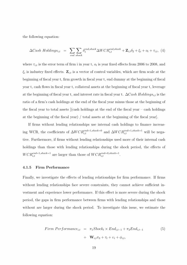
∆Cash Holdingsi,t =∑end

∑shock

δend,shock1 ∆WCRend,shock

i,t + Zi,tδ2 + ξi + ot + τi,t, (4)

where τi,t is the error term of firm i in year t, ot is year fixed effects from 2006 to 2008, and

ξi is industry fixed effects. Zi,t is a vector of control variables, which are firm scale at the

beginning of fiscal year t, firm growth in fiscal year t, end dummy at the beginning of fiscal

year t, cash flows in fiscal year t, collateral assets at the beginning of fiscal year t, leverage

at the beginning of fiscal year t, and interest rate in fiscal year t. ∆Cash Holdingsi,t is the

ratio of a firm’s cash holdings at the end of the fiscal year minus those at the beginning of

the fiscal year to total assets [(cash holdings at the end of the fiscal year – cash holdings

at the beginning of the fiscal year) / total assets at the beginning of the fiscal year].

If firms without lending relationships use internal cash holdings to finance increas-

ing WCR, the coefficients of ∆WCRend=1,shock=0i,t and ∆WCRend=1,shock=1

i,t will be nega-

tive. Furthermore, if firms without lending relationships used more of their internal cash

holdings than those with lending relationships during the shock period, the effects of

WCRend=1,shock=1i,t are larger than those of WCRend=0,shock=1

i,t .

4.1.5 Firm Performance

Finally, we investigate the effects of lending relationships for firm performance. If firms

without lending relationships face severe constraints, they cannot achieve sufficient in-

vestment and experience lower performance. If this effect is more severe during the shock

period, the gaps in firm performance between firms with lending relationships and those

without are larger during the shock period. To investigate this issue, we estimate the

following equation:

Firm Performancei,t = π1Shockt × Endi,t−1 + π2Endi,t−1 (5)

+ Wi,tπ3 + τt + υi + ϕi,t,

19

where ϕi,t is the error term of firm i in year t, τt is year fixed effects from 2006 to 2008,

and υi is industry fixed effects. Wi,t is a vector of control variables, which comprise firm

scale at the beginning of fiscal year t, firm growth in fiscal year t, collateral assets at

the beginning of fiscal year t, and leverage at the beginning of fiscal year t. Shockt is a

dummy variable that equals one if the fiscal year is 2008, and zero otherwise. Endi,t−1 is

an end dummy at the beginning of fiscal year t.

Our sample data are for small businesses, which are mainly unlisted firms. Therefore,

we cannot acquire stock data, such as stock prices and firm values. Many previous studies

use Tobin’s q or stock returns as a proxy of firm performance. However, these data are

unavailable for small businesses. Instead, we use accounting profitability as a proxy of

firm performance, defined as the ratio of a firm’s operating income to total assets. If firms

without lending relationships face severe constraints, they experience lower performance

after the shock. As a result, the coefficients of Shockt × Endi,t−1 (π1) will be negative if

the lending relationships are valuable.12

4.2 Results

4.2.1 Bank Borrowings

Table 9 shows summary statistics for the variables in equations (2)–(5). Table 10 shows

the estimation results for equation (2) using total bank borrowings as a dependent vari-

able. In column (1), all estimated coefficients of ∆WCR are positive and statistically

significant. These results imply that both types of firms increased bank borrowings dur-

ing the nonshock and shock periods when they faced the increased WCR. Focusing on

the magnitude of the estimated coefficients of ∆WCR, we see a difference between firms

with lending relationships and those without. The estimated coefficients of ∆WCR for

firms ending relationships are smaller than those with relationships, suggesting that firms

12Some data of firm performance in fiscal year t+1 are unavailable. Therefore, we focus only onshort-term performance.

20

without lending relationships increase their bank borrowings by less to finance WCR.

In addition, the estimated coefficient of ∆WCR for firms without lending relationships

during the shock period is the smallest.

To investigate the heterogeneous effects between small and medium firms, we divide

the sample into two groups. The definitions of small and medium firms are the same as

in those used in Subsection 3.2. In column (2), we show the results for medium firms.

All estimated coefficients of ∆WCR are similar to those in column (1), suggesting that

firms increase bank borrowings when they face higher WCR. Furthermore, firms without

lending relationships increase their bank borrowings by less. In column (3), we limit the

sample to small firms. The signs of all estimated coefficients of ∆WCR are positive, but

that of ∆WCRend=1,shock=1 is not statistically significant. This suggests that small firms

without lending relationships did not significantly increase bank borrowings during the

shock period when they faced higher WCR.

In sum, the estimation results of Table 10 imply that firms increased bank borrowings

in both the shock and nonshock periods even if they ended their lending relationships.

However, the amount of bank borrowings is smaller for firms without such relationships.

In particular, the increase in bank borrowings is insignificant for small firms without

lending relationships during the shock period. These results might imply that credit

constraints are severe for firms without relationships. They also imply that firms without

lending relationships do not increase bank borrowings because they have enough liquidity

to finance credit demand.

The negative effects of cash flow suggest that firms with low liquidity increase bank

borrowings. The effects of firm scale and firm growth are positive because they have high

credit demand and are relatively informationally transparent. The effects of collateral

assets are negative, suggesting that firms with more collateral assets decreased their bank

borrowings. In general, credit supply for those firms is high, so the effects of collateral

assets should be positive. However, the estimated results are inconsistent with this view.

21

Furthermore, the effects of interest rates are positive (not negative). A possible reason

for these results is that credit demands in firms with lower collateral and higher interest

rates are high.

4.2.2 Interest Rates

To investigate whether credit constraints are severe for firms without relationships, we

estimate equation (3) using interest rates as a dependent variable. Table 11 shows the

estimated results for equation (3). All coefficients of ∆WCR are statistically insignificant.

This implies that firms do not pay higher interest rates to finance working capital. This

result is similar for firms without lending relationships during the shock period. If firms

without lending relationships face severe credit constraints, they should pay higher interest

rates especially during the financial shock. As a result, the coefficient of WCRend=1,shock=1i,t

should be positive. The estimated results imply that firms without lending relationships

do not face severe credit constraints. The results in columns (2) and (3) are for the

small and medium firms, respectively. Similar to column (1), all estimated coefficients of

∆WCR are statistically insignificant, apart from WCRend=0,shock=1i,t in column (2). The

magnitude of the coefficient is –0.0067, suggesting that the economic significance is weak.

Some of the coefficients of firm scale and collateral assets are positive and statistically

significant. Larger-sized small businesses and firms with more collateral assets are rela-

tively creditworthy, so interest rates for those firms should be lower. On the other hand,

they can borrow for longer maturities, so the cost of loans may become higher. As highly

leveraged firms are risky for creditors, the effects of leverage are positive and statistically

significant.

4.2.3 Cash Holdings

Table 12 shows the estimation results using cash holdings as a dependent variable. All

estimated coefficients of ∆WCR are negative and statistically significant at the 1% level,

22

implying that both firms with lending relationships and those without reduce their cash

holdings when they face WCR. The magnitude of the estimated coefficients for firms with-

out lending relationships during both the nonshock and shock periods (∆WCRend=1,shock=0

and ∆WCRend=1,shock=1) is larger than for those with lending relationships. This result

suggests that firms without lending relationships reduce their cash holdings by more when

they face WCR. In addition, the effect of ∆WCR is the largest in firms without lending

relationships during the shock period. These firms use internal cash during the shock

period to finance working capital requirements, instead of bank borrowings.

In Table 12, we show the results for medium firms in column (2), and small firms

in column (3). Similar to the results using all observations in column (1), all estimated

coefficients of ∆WCR are negative and statistically significant at the 1% level. The dif-

ference in ∆WCR between firms with lending relationships and those without is larger

in small firms. Our estimated results suggest that small firms without lending relation-

ships reduced their internal cash holdings by more to finance increasing WCR, instead of

increasing their bank borrowings during the shock period.

4.2.4 Operating Income

Column (1) of Table 13 shows the estimation results of equation (5) using all observations.

The estimated coefficient of the shock dummy is negative and statistically significant at

the 1% level, suggesting that operating income for small businesses declines after the

shock period. The estimated coefficient of the end dummy is not statistically significant.

To investigate whether firms without lending relationships experienced lower performance

after the shock, we focus on the coefficient of shock × end dummy. If their performance is

lower, this coefficient will be negative. The estimated coefficient for the interactive variable

is negative, but not statistically significant. This result implies that firms without lending

relationships experienced significantly lower performance after the shock. Furthermore,

credit constraints for firms without relationships are not severe.

23

Columns (2) and (3) show the results using only small and medium firms. For both

groups of firms, the estimated coefficients of the shock dummy are negative and statis-

tically significant. The results for the end dummy are mixed: negative for small firms

and positive for medium firms. The estimated coefficients of the shock × end dummy

are not statistically significant, which is similar to the results using all observations. The

results for the control variables show that the performance of larger firms, growing firms,

and low leveraged firms is high. Furthermore, collateral assets have negative effects on

performance except for small firms.

4.3 Propensity Score Matching

4.3.1 Constraints or Adequate Liquidity?

In the previous section, we showed that firms without lending relationships relied less on

bank borrowings and more on internal cash holdings to finance credit demand during the

financial shock period. These results imply that as firms without lending relationships

did not use bank loans during the shock period, they reduced cash holdings to finance

credit demand. These results also imply that these firms did not use bank loans because

they had adequate cash holdings. The latter interpretation is consistent with a pecking

order theory, which shows that firms use internal firm cash, and they borrow from outside

lenders after exhausting their cash. This interpretation supports the result that they

faced higher interest rates during the shock period.

It is also not clear whether firms with lending relationships increase bank borrow-

ings if they have enough internal cash. Table 14 shows the median growth rates of total

bank borrowings and cash holdings during the financial shock period (FY2008), sepa-

rated according to the amount of cash holdings and whether or not the firms have lending

relationships. To limit our analysis to only those firms having credit demand, only obser-

vations with positive ∆WCR are used in this table.

Panel A shows the results for bank borrowings. When we focus on the column with

24

the highest ∆WCR, the differences in bank borrowings between firms with relationships

and those without are statistically significant in rows 1 to 3. In contrast, in row 4,

the difference is not statistically significant, suggesting that firms with relationships do

not increase their bank borrowings by more. Panel B shows the median growth rate of

cash holdings. Focusing on the column with the largest ∆WCR, the growth rate of cash

holdings in firms without relationships is smaller than in those with relationships in rows

1 to 3. In contrast, the difference is statistically insignificant in row 4, which is the group

of firms having the largest cash holdings. These results suggest that cash-rich firms used

internal cash to finance working capital during the shock period even if they had lending

relationships.

4.3.2 Estimation Strategy

To investigate which explanations are plausible, we employ the propensity score matching

method, first introduced by Rosenbaum and Rubin (1983). As we showed in Section

3, firms decide whether or not to continue lending relationships, which implies that the

end dummy is an endogenous variable. Furthermore, firms with large cash holdings are

likely to end their relationships. By using simple regressions using an end dummy, we

can compare firms that are cash rich and those that are cash poor. The propensity score

matching method helps mitigate the endogeneity problem.

The propensity score is the probability of receiving treatment, which in our paper is

the probability of ending lending relationships. To calculate the propensity score p(Vi,t),

we estimate the probability of ending lending relationships using the following probit

model:

p(Vi,FY 2007) ≡ P (Endi,FY 2007 = 1 | Vi,FY 2007) = Φ(Vi,FY 2007ρ), (6)

where Vi,FY 2007 = (Cash Holdingsi,FY 2006, Cash F lowi,FY 2007, F irm Sizei,FY 2007,

F irm Growthi,FY 2007, Endi,FY 2006, IndustryDummy). The definitions of variables Vi,FY 2007

25

are the same as in Section 3. To satisfy the balancing property, we omit the tangible fixed

assets and WCR from the equation. Φ is the cumulative distribution function of the

standard normal distribution. As we now employ outcome variables in fiscal year t+1, we

limit the observations to those where the outcome variables in FY2008 are available. The

number of observations is 1,671. We compare the periods before and after the financial

shock in 2008. We estimate the determinants of ending relationships in FY2007, which

means that the treatment and control groups are determined before the financial shock.

The estimation results for equation (6) are as follows.

P (Endi,FY 2007 = 1 | Vi,FY 2007) = Φ(−0.147 + 0.771 × Cash Holdingsi,FY 2006

+ 1.481 × Cash F lowi,FY 2007 − 0.071 × Firm Sizei,FY 2006

− 1.447 × Firm Growthi,FY 2007

+ 3.865 × Endi,FY 2006) (7)

The estimation results are similar to those in Table 6. All coefficients apart from firm

scale are statistically significant. Using the estimated coefficients in equation (7), we

calculate the estimated propensity score [p(Vi,FY 2007)] for each observation, and match the

observations based on the estimated propensity score. We employ a k -nearest neighbor-

matching algorithm to match the treatment and control observations where k indicates the

number of control observations matched with each treatment observation. We estimate the

propensity score by matching each treatment observation using its five nearest neighbors.

To check whether the matching is suitable, we use the balancing test. First, we test

the difference in the mean of each variable between the treated and matched observations.

The means of each variable are shown in Table 15. Before matching, the differences of

all variables apart from firm size and growth between treated and unmatched control

observations are statistically significant at the 1% level. This suggests that the charac-

teristics are not similar between firms with lending relationships and those without. The

26

differences between the treated and matched control observations are not statistically sig-

nificant apart from firm growth and scale, so we fail to reject the null hypothesis that

the differences in the means between the treated and matched control observations are

zero. This suggests that after matching, the differences in characteristics between the

treated and control observations are small. In particular, the differences in cash flows

and holdings between the treated and matched control firms are statistically insignificant,

so that both firms with lending relationships and those without have large internal cash

holdings. Second, we estimate equation (6) using only the treated and matched control

observations. Before matching, the pseudo R2 value for the estimate of equation (6) is

0.779. After matching, the pseudo R2 value for equation (6) decreases to 0.009, which

is lower than that in the model using all observations. These results suggest that the

differences between the treated and matched observations are not significantly large.

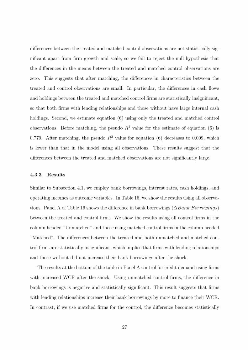
4.3.3 Results

Similar to Subsection 4.1, we employ bank borrowings, interest rates, cash holdings, and

operating incomes as outcome variables. In Table 16, we show the results using all observa-

tions. Panel A of Table 16 shows the difference in bank borrowings (∆Bank Borrowings)

between the treated and control firms. We show the results using all control firms in the

column headed “Unmatched” and those using matched control firms in the column headed

“Matched”. The differences between the treated and both unmatched and matched con-

trol firms are statistically insignificant, which implies that firms with lending relationships

and those without did not increase their bank borrowings after the shock.

The results at the bottom of the table in Panel A control for credit demand using firms

with increased WCR after the shock. Using unmatched control firms, the difference in

bank borrowings is negative and statistically significant. This result suggests that firms

with lending relationships increase their bank borrowings by more to finance their WCR.

In contrast, if we use matched firms for the control, the difference becomes statistically

27

insignificant. This result implies that both firms with lending relationships and those

without them increased their borrowings by only small amounts.13

Panel B of Table 16 shows the results using interest rates as an outcome variable. To

control for the differences between the control and matched firms, we show the difference-

in-differences parameters, which measure the net effects of the financial shock for the

treated firms. The differences in interest rates between the treated and unmatched control

firms are statistically significant before and after the shock. If we use matched firms, the

differences are significant only before the shock using all observations. The difference-in-

differences is statistically insignificant if we compare treated firms and matched control

firms, implying that firms without lending relationships do not face more severe credit

constraints. The bottom of Panel B shows the results using firms that faced increasing

WCR. The results are similar to those using all observations.

Panel C of Table 16 shows the results using cash holdings (∆Cash Holdings) as an

outcome variable. Using all observations, the difference between the matched control

and treated firms is statistically insignificant before the financial shock. The bottom of

Panel C shows the results using firms with increasing WCR. The difference-in-differences

is negative and statistically significant for unmatched control firms. If we use unmatched

firms for controls, we see that the treated firms reduced their cash holdings by more than

control firms after the shock. On the other hand, if we use matched firms for controls,

the difference-in-differences of cash holdings is not statistically significant. Furthermore,

the average cash holdings after the shock are negative in both the treated and matched

control firms, suggesting that they reduced their cash holdings to increase their capital

during the shock period.

In Section 4, using simple regressions, we showed that firms without lending relation-

ships increased their bank borrowings by less and reduced their internal cash by more

13As Table 15 shows, many matched firms with lending relationships were unlikely to have relationshipsat the beginning of FY2007. Therefore, the growth rates of bank borrowings should be large in FY2007.As a result, the difference-in-differences of bank borrowings for matched firms becomes negative. We onlyshow the difference in growth rates of bank borrowings in Table 16.

28

to finance their WCR during the shock period. The results from the propensity score

matching do not support these results, implying that if firms have adequate internal

cash holdings, both firms with lending relationships and those without did not use bank

borrowings and reduced their cash holdings during the shock period.

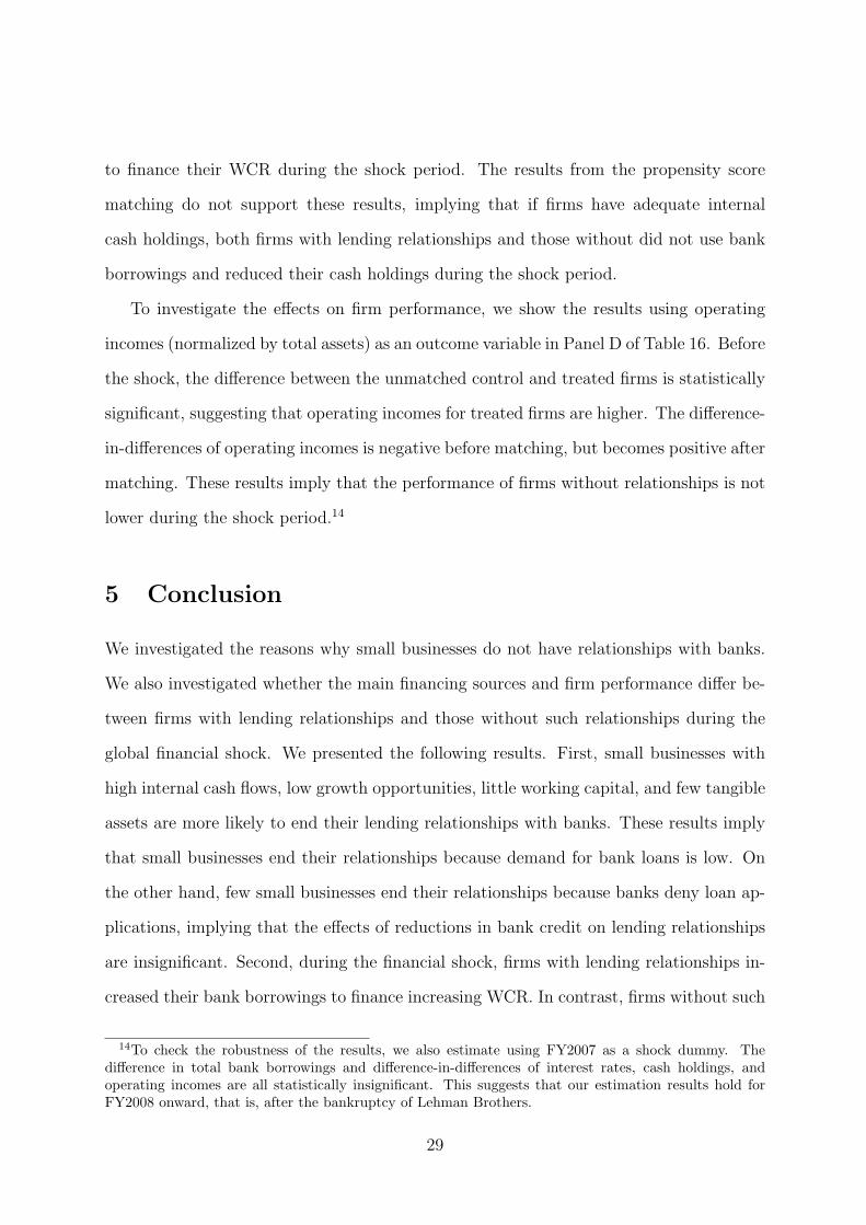
To investigate the effects on firm performance, we show the results using operating

incomes (normalized by total assets) as an outcome variable in Panel D of Table 16. Before

the shock, the difference between the unmatched control and treated firms is statistically

significant, suggesting that operating incomes for treated firms are higher. The difference-

in-differences of operating incomes is negative before matching, but becomes positive after

matching. These results imply that the performance of firms without relationships is not

lower during the shock period.14

5 Conclusion

We investigated the reasons why small businesses do not have relationships with banks.

We also investigated whether the main financing sources and firm performance differ be-

tween firms with lending relationships and those without such relationships during the

global financial shock. We presented the following results. First, small businesses with

high internal cash flows, low growth opportunities, little working capital, and few tangible

assets are more likely to end their lending relationships with banks. These results imply

that small businesses end their relationships because demand for bank loans is low. On

the other hand, few small businesses end their relationships because banks deny loan ap-

plications, implying that the effects of reductions in bank credit on lending relationships

are insignificant. Second, during the financial shock, firms with lending relationships in-

creased their bank borrowings to finance increasing WCR. In contrast, firms without such

14To check the robustness of the results, we also estimate using FY2007 as a shock dummy. Thedifference in total bank borrowings and difference-in-differences of interest rates, cash holdings, andoperating incomes are all statistically insignificant. This suggests that our estimation results hold forFY2008 onward, that is, after the bankruptcy of Lehman Brothers.

29

relationships reduced their cash holdings, rather than increasing their bank borrowings.

Cash-rich firms used internal cash holdings even if they had lending relationships. This

result implies that firms prefer internal cash holdings, which is consistent with a pecking

order theory. Third, the differences in performance (in terms of profitability) between

firms having relationships and those not having relationships are insignificant during the

shock period, implying that credit constraints for firms without relationships are not

severe.

After the Financial Services Agency adopted the Action Program Concerning En-

hancement of Relationship Banking Functions in 2003, close relationships between banks

and small businesses were promoted by the government. Our estimated results show that

small businesses with high liquidity end lending relationships with banks, implying that

they have no need for such relationships. Furthermore, they have enough liquidity to

finance credit demand during the unexpected shock period, so the credit constraints are

not severe. Therefore, the policy effects on the strength of lending relationships for small

businesses with low demand for bank loans are insignificant. On the other hand, some

small businesses have neither sufficient cash holdings nor lending relationships. As Table

14 shows, small businesses with low liquidity and no relationships do not increase bank

borrowings and reduce cash holdings when they face high credit demand. The credit

constraints for these firms might be severe, so there might be a need to enhance credit

supply for these firms by public credit guarantee or government lending.

30

References

Bates, T. W., Kahle, K. M., Stulz, R. M., 2009. Why do U.S. firms hold so much more

cash than they used to? Journal of Finance 64 (5), 1985–2021.

Berger, A. N., Udell, G. F., 1995. Lines of credit and relationship lending in small firm

finance. Journal of Business 68 (3), 351–381.

Berlin, M., Mester, L., 1999. Deposits and relationship lending. Review of Financial Stud-

ies 12 (3), 579–607.

Boot, A. W. A., 2000. Relationship banking: What do we know? Journal of Financial

Intermediation 9 (1), 7–25.

Campello, M., Giambona, E., Graham, J. R., Harvey, C. R., 2011. Liquidity management

and corporate investment during a financial crisis. Review of Financial Studies 24 (6),

1944–1979.

Campello, M., Giambona, E., Graham, J. R., Harvey, C. R., 2012. Access to liquidity and

corporate investment in Europe during the financial crisis. Review of Finance 16 (2),

323–346.

Cole, R. A., 2010. Bank credit, trade credit or no credit? evidence from the surveys of

small business finances, U.S. Small Business Administration Research Study, No.365.

Cotugno, M., Monferra, S., Sampagnaro, G., 2013. Relationship lending, hierarchical

distance and credit tightening: Evidence from the financial crisis. Journal of Banking

& Finance 37 (5), 1372 – 1385.

Dewally, M., Shao, Y., 2014. Liquidity crisis, relationship lending and corporate finance.

Journal of Banking & Finance 39, 223 – 239.

Gobbi, G., Sette, E., 2014. Do firms benefit from concentrating their borrowing? Evidence

from the great recession. Review of Finance Forthcoming.

31

Hill, M. D., Kelly, G. W., Highfield, M. J., 2010. Net operating working capital behavior:

A first look. Financial Management 39 (2), 783–805.

Hoshi, T., Kashyap, A., Scharfstein, D., 1991. Corporate structure, liquidity, and invest-

ment: Evidence from Japanese industrial groups. The Quarterly Journal of Economics

106 (1), 33–60.

Jiangli, W., Unal, H., Yom, C., 2008. Relationship lending, accounting disclosure, and

credit availability during the Asian financial crisis. Journal of Money, Credit and Bank-

ing 40 (1), 25–55.

Miwa, Y., 2012. Are Japanese firms becoming more independent from their banks?: Evi-

dence from the firm-level data of the “corporate enterprise quarterly statistics,” 1994-

2009. Public Policy Review 8 (4), 415–452.

Ongena, S., Smith, D. C., 2001. The duration of bank relationships. Journal of Financial

Economics 61 (3), 449–475.

Petersen, M., Rajan, R. G., 1994. The benefits of firm-creditor relationships: Evidence

from small business data. Journal of Finance 49 (1), 3–37.

Preve, L. A., Sarria-allende, V., 2010. Working Capital Management. Oxford University

Press, London.

Rosenbaum, P. R., Rubin, D. B., 1983. The central role of the propensity score in obser-

vational studies for causal effects. Biometrica 70 (1), 41–55.

Slovin, M. B., Sushka, M. E., Polonchek, J. A., 1993. The value of bank durability:

Borrowers as bank stakeholders. Journal of Finance 48 (1), 247–66.

Small and Medium Enterprise Agency, 2007. The 2007 White Paper on Small and Medium

Enterprises in Japan: Harnessing Regional Strengths and Confronting the Changes.

32

Sohn, W., 2010. Market response to bank relationships: Evidence from Korean bank

reform. Journal of Banking & Finance 34 (9), 2042 – 2055.

Strebulaev, I. A., Yang, B., 2013. The mystery of zero-leverage firms. Journal of Financial

Economics 109 (1), 1 – 23.

Tsuruta, D., Uchida, H., 2013. Real Driver of Trade Credit. Discussion papers 13-E-037,

Research Institute of Economy, Trade and Industry (RIETI).

Uchino, T., 2013. Bank dependence and financial constraints on investment: Evidence

from the corporate bond market paralysis in Japan. Journal of the Japanese and Inter-

national Economies 29, 74 – 97.

Yamori, N., Murakami, A., 1999. Does bank relationship have an economic value?: The

effect of main bank failure on client firms. Economics Letters 65 (1), 115–120.

33

Table 1: Number of Observations, by Firm Size and Year

Employees -20 21-100 101-300 301-500 Total2001 3,080 3,235 2,081 564 8,9602002 3,274 3,238 2,080 549 9,1412003 3,528 3,413 2,214 535 9,6902004 3,663 3,673 2,289 622 10,2472005 3,776 3,576 2,292 567 10,2112006 3,706 3,644 2,256 560 10,1662007 3,558 3,487 2,288 577 9,9102008 3,601 3,405 2,209 573 9,788

Note: This table shows the number of observations divided by year and number of employees.

Table 2: Distribution of Total Bank Borrowings (Normalized by Total Assets)

p25 Median p752001 0.00 24.30 50.422002 0.00 22.76 48.602003 0.00 19.07 46.042004 0.00 17.61 44.422005 0.00 15.61 43.692006 0.00 14.49 42.362007 0.00 13.54 42.012008 0.00 12.88 42.94

Note: This table shows the quartiles of total bank borrowings, normalized by total assets at the end ofthe fiscal year. The numbers are expressed in percentage terms.

Table 3: Median of Total Bank Borrowings (Normalized by Total Assets), by Firm Size

Employees -20 21-100 101-300 301- Total2001 18.67 28.13 24.86 23.97 24.302002 17.11 26.28 23.75 20.52 22.762003 15.00 22.91 18.32 17.73 19.072004 14.22 21.83 17.86 11.86 17.612005 12.02 20.56 15.07 10.24 15.612006 9.24 19.88 15.00 7.79 14.492007 10.49 17.57 12.87 7.80 13.542008 10.53 16.67 12.23 5.62 12.88

Note: This table shows the median of total bank borrowings (normalized by total assets) at the end ofthe fiscal year, divided by the number of employees. The numbers are expressed in percentage terms.

34

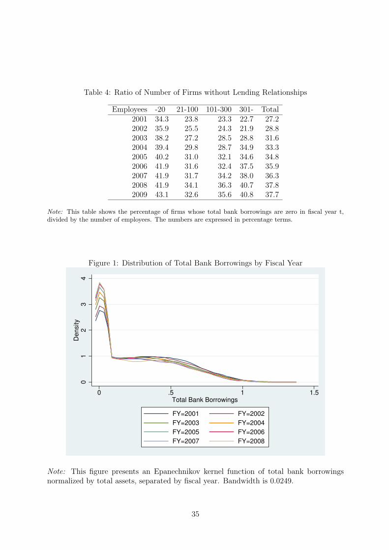
Table 4: Ratio of Number of Firms without Lending Relationships

Employees -20 21-100 101-300 301- Total2001 34.3 23.8 23.3 22.7 27.22002 35.9 25.5 24.3 21.9 28.82003 38.2 27.2 28.5 28.8 31.62004 39.4 29.8 28.7 34.9 33.32005 40.2 31.0 32.1 34.6 34.82006 41.9 31.6 32.4 37.5 35.92007 41.9 31.7 34.2 38.0 36.32008 41.9 34.1 36.3 40.7 37.82009 43.1 32.6 35.6 40.8 37.7

Note: This table shows the percentage of firms whose total bank borrowings are zero in fiscal year t,divided by the number of employees. The numbers are expressed in percentage terms.

Figure 1: Distribution of Total Bank Borrowings by Fiscal Year

01

23

4D

ensi

ty

0 .5 1 1.5Total Bank Borrowings

FY=2001 FY=2002FY=2003 FY=2004FY=2005 FY=2006FY=2007 FY=2008

Note: This figure presents an Epanechnikov kernel function of total bank borrowingsnormalized by total assets, separated by fiscal year. Bandwidth is 0.0249.

35

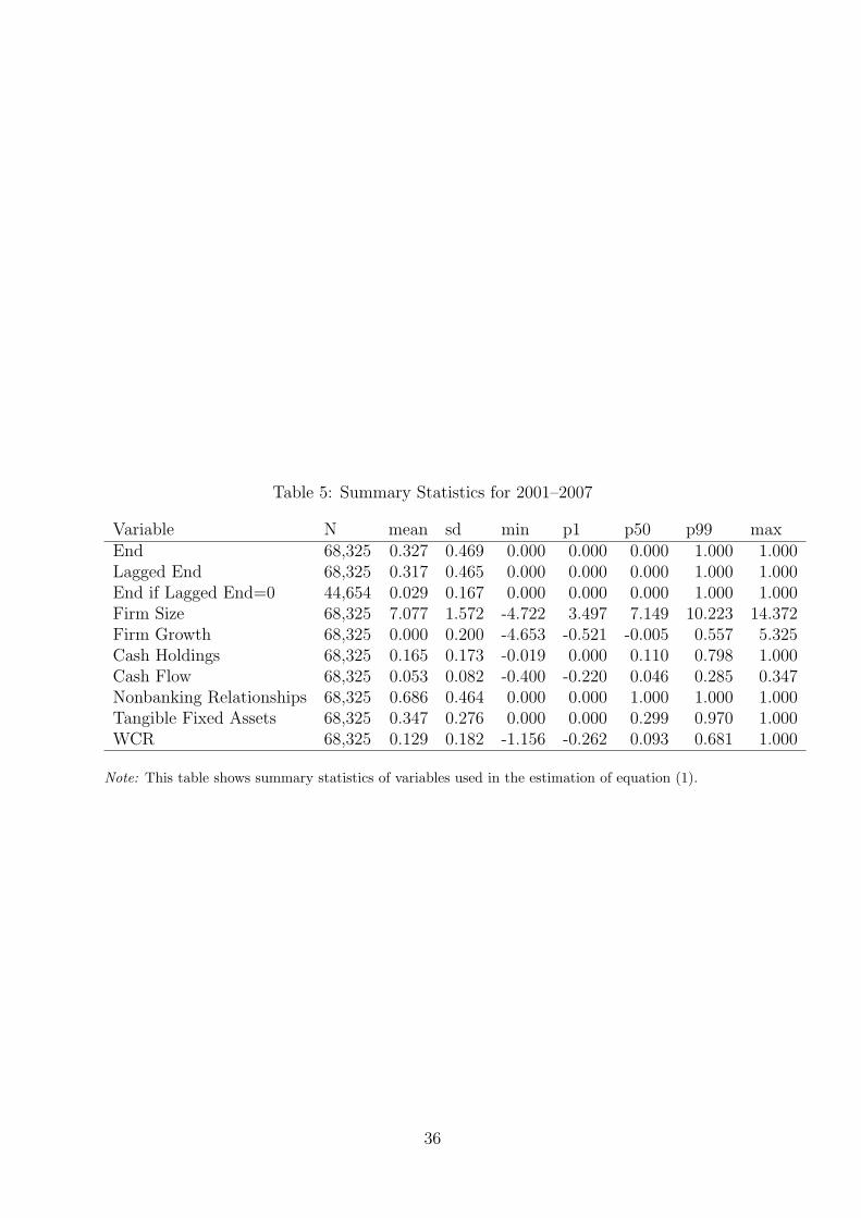
Table 5: Summary Statistics for 2001–2007

Variable N mean sd min p1 p50 p99 maxEnd 68,325 0.327 0.469 0.000 0.000 0.000 1.000 1.000Lagged End 68,325 0.317 0.465 0.000 0.000 0.000 1.000 1.000End if Lagged End=0 44,654 0.029 0.167 0.000 0.000 0.000 1.000 1.000Firm Size 68,325 7.077 1.572 -4.722 3.497 7.149 10.223 14.372Firm Growth 68,325 0.000 0.200 -4.653 -0.521 -0.005 0.557 5.325Cash Holdings 68,325 0.165 0.173 -0.019 0.000 0.110 0.798 1.000Cash Flow 68,325 0.053 0.082 -0.400 -0.220 0.046 0.285 0.347Nonbanking Relationships 68,325 0.686 0.464 0.000 0.000 1.000 1.000 1.000Tangible Fixed Assets 68,325 0.347 0.276 0.000 0.000 0.299 0.970 1.000WCR 68,325 0.129 0.182 -1.156 -0.262 0.093 0.681 1.000

Note: This table shows summary statistics of variables used in the estimation of equation (1).

36

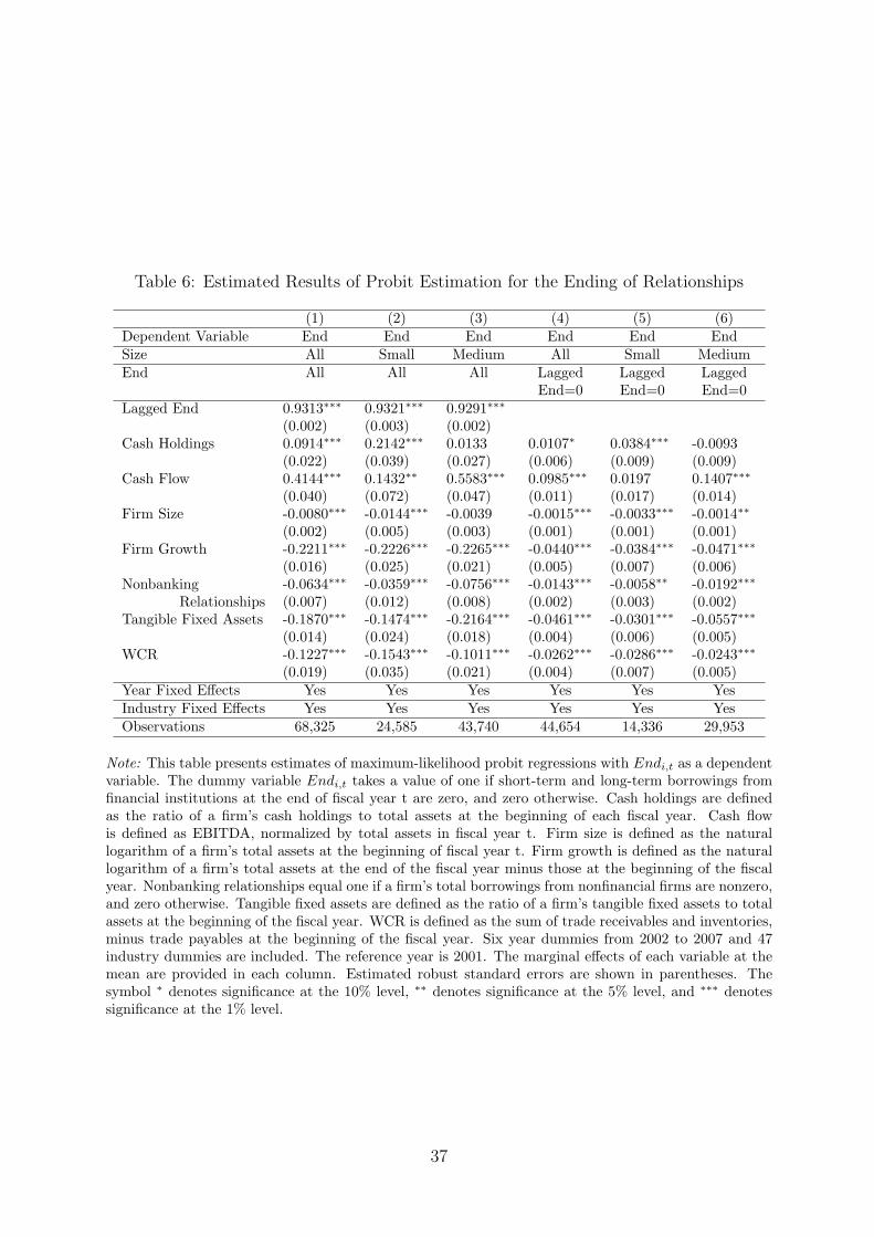
Table 6: Estimated Results of Probit Estimation for the Ending of Relationships

(1) (2) (3) (4) (5) (6)Dependent Variable End End End End End EndSize All Small Medium All Small MediumEnd All All All Lagged Lagged Lagged

End=0 End=0 End=0Lagged End 0.9313∗∗∗ 0.9321∗∗∗ 0.9291∗∗∗

(0.002) (0.003) (0.002)Cash Holdings 0.0914∗∗∗ 0.2142∗∗∗ 0.0133 0.0107∗ 0.0384∗∗∗ -0.0093

(0.022) (0.039) (0.027) (0.006) (0.009) (0.009)Cash Flow 0.4144∗∗∗ 0.1432∗∗ 0.5583∗∗∗ 0.0985∗∗∗ 0.0197 0.1407∗∗∗

(0.040) (0.072) (0.047) (0.011) (0.017) (0.014)Firm Size -0.0080∗∗∗ -0.0144∗∗∗ -0.0039 -0.0015∗∗∗ -0.0033∗∗∗ -0.0014∗∗

(0.002) (0.005) (0.003) (0.001) (0.001) (0.001)Firm Growth -0.2211∗∗∗ -0.2226∗∗∗ -0.2265∗∗∗ -0.0440∗∗∗ -0.0384∗∗∗ -0.0471∗∗∗

(0.016) (0.025) (0.021) (0.005) (0.007) (0.006)Nonbanking -0.0634∗∗∗ -0.0359∗∗∗ -0.0756∗∗∗ -0.0143∗∗∗ -0.0058∗∗ -0.0192∗∗∗

Relationships (0.007) (0.012) (0.008) (0.002) (0.003) (0.002)Tangible Fixed Assets -0.1870∗∗∗ -0.1474∗∗∗ -0.2164∗∗∗ -0.0461∗∗∗ -0.0301∗∗∗ -0.0557∗∗∗

(0.014) (0.024) (0.018) (0.004) (0.006) (0.005)WCR -0.1227∗∗∗ -0.1543∗∗∗ -0.1011∗∗∗ -0.0262∗∗∗ -0.0286∗∗∗ -0.0243∗∗∗

(0.019) (0.035) (0.021) (0.004) (0.007) (0.005)Year Fixed Effects Yes Yes Yes Yes Yes YesIndustry Fixed Effects Yes Yes Yes Yes Yes YesObservations 68,325 24,585 43,740 44,654 14,336 29,953

Note: This table presents estimates of maximum-likelihood probit regressions with Endi,t as a dependentvariable. The dummy variable Endi,t takes a value of one if short-term and long-term borrowings fromfinancial institutions at the end of fiscal year t are zero, and zero otherwise. Cash holdings are definedas the ratio of a firm’s cash holdings to total assets at the beginning of each fiscal year. Cash flowis defined as EBITDA, normalized by total assets in fiscal year t. Firm size is defined as the naturallogarithm of a firm’s total assets at the beginning of fiscal year t. Firm growth is defined as the naturallogarithm of a firm’s total assets at the end of the fiscal year minus those at the beginning of the fiscalyear. Nonbanking relationships equal one if a firm’s total borrowings from nonfinancial firms are nonzero,and zero otherwise. Tangible fixed assets are defined as the ratio of a firm’s tangible fixed assets to totalassets at the beginning of the fiscal year. WCR is defined as the sum of trade receivables and inventories,minus trade payables at the beginning of the fiscal year. Six year dummies from 2002 to 2007 and 47industry dummies are included. The reference year is 2001. The marginal effects of each variable at themean are provided in each column. Estimated robust standard errors are shown in parentheses. Thesymbol ∗ denotes significance at the 10% level, ∗∗ denotes significance at the 5% level, and ∗∗∗ denotessignificance at the 1% level.

37

Table 7: Estimated Results of Probit Estimation for the Ending of Relationships UsingFinancial DI

(1) (2) (3) (4) (5) (6)Dependent Variable End End End End End EndSize All Small Medium All Small MediumEnd All All All Lagged Lagged Lagged

End=0 End=0 End=0Financial DI -0.0006∗ -0.0009 -0.0005 -0.0000 -0.0000 -0.0001

(0.000) (0.001) (0.000) (0.000) (0.000) (0.000)Year Fixed Effects Yes Yes Yes Yes Yes YesIndustry Fixed Effects No No No No No NoObservations 66,306 23,384 42,922 43,239 13,658 29,581

Note: This table presents estimates of maximum-likelihood probit regressions with Endi,t as the de-pendent variable. We estimate equation (1) using financial DI as an additional dependent variable. Theestimated coefficients of other variables are omitted. The marginal effects of each variable at the mean areprovided in each column. The estimated robust standard errors are shown in parentheses. The symbol ∗

denotes significance at the 10% level, ∗∗ denotes significance at the 5% level, and ∗∗∗ denotes significanceat the 1% level.

Table 8: Responses of Loan Applications to Main Banks and Lending RelationshipsAns. 1 Ans. 2 Ans. 3 Ans. 4 Ans. 5 Ans. 6 Freq..

Continue 5.53 34.22 12.84 6.88 9.60 30.93 7,727End 0.37 0.09 0.00 0.00 0.00 99.54 1,087Total 4.89 30.01 11.25 6.04 8.42 39.39 8,814

Note: The numbers are expressed in percentages. The possible responses are 1) Applications rejected oramounts requested reduced, 2) Could borrow amounts requested without changes in borrowing terms, 3)Borrowing terms severe, but could borrow amounts requested, 4) Could borrow amounts requested aftereasing of borrowing terms, 5) Bank suggested increasing loan amount, and 6) Have not submitted loanapplications.

38

Table 9: Summary Statistics for 2006–2008

Variable N mean sd min p1 p50 p99 maxInterest Rate 29,864 0.015 0.016 0.000 0.000 0.014 0.067 0.172Total Bank Borrowings 29,864 -0.002 0.059 -0.258 -0.174 0.000 0.199 0.305Cash Holdings 29,864 -0.002 0.079 -1.000 -0.262 0.000 0.215 0.989Operating Income 29,679 0.022 0.077 -0.448 -0.265 0.021 0.219 0.270∆ WCR 29,864 0.004 0.072 -0.270 -0.205 0.000 0.246 0.352Firm Growth 29,864 -0.006 0.195 -4.653 -0.548 -0.006 0.542 5.325Firm Size 29,864 7.080 1.590 -3.533 3.434 7.153 10.282 14.273Cash Flow 29,864 0.053 0.086 -0.400 -0.235 0.046 0.290 0.347Leverage 29,864 0.640 0.308 0.000 0.008 0.677 1.512 2.162Collateral Assets 29,864 0.338 0.276 0.000 0.000 0.287 0.968 1.000End 29,864 0.359 0.480 0.000 0.000 0.000 1.000 1.000

Note: This table shows summary statistics of variables used in the estimation of equations (2), (3), (4),and (5).

39

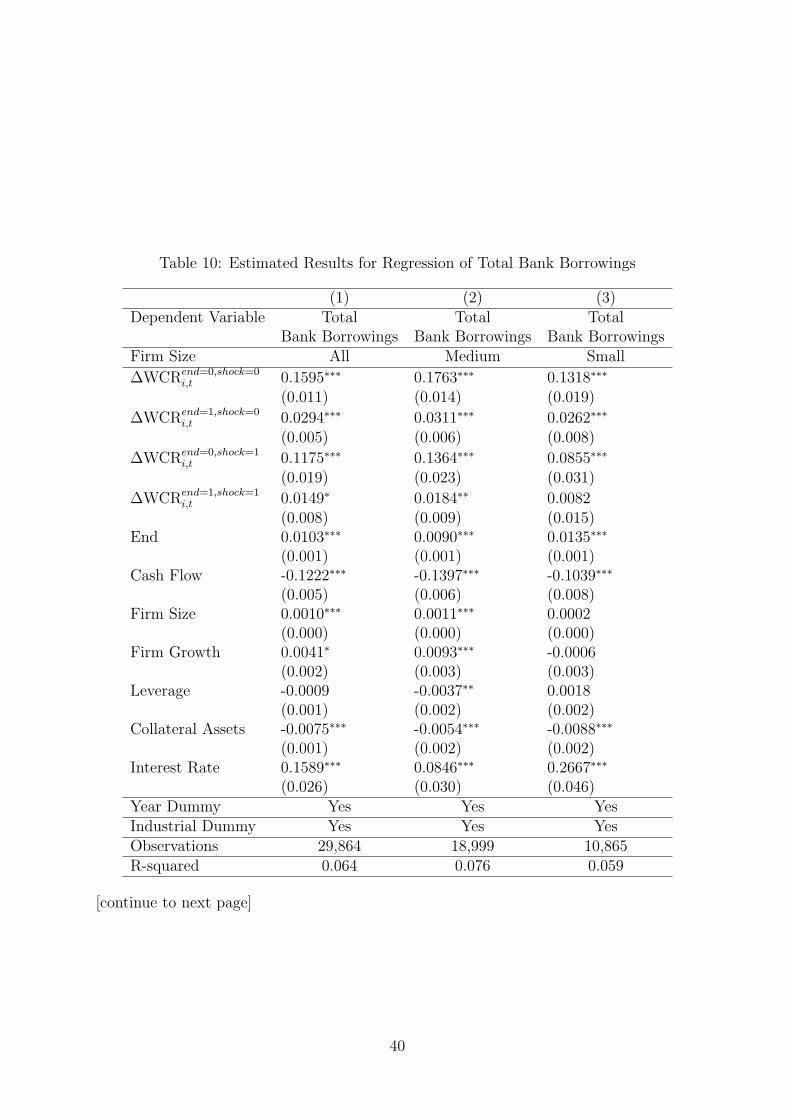
Table 10: Estimated Results for Regression of Total Bank Borrowings

(1) (2) (3)Dependent Variable Total Total Total

Bank Borrowings Bank Borrowings Bank BorrowingsFirm Size All Medium Small

∆WCRend=0,shock=0i,t 0.1595∗∗∗ 0.1763∗∗∗ 0.1318∗∗∗

(0.011) (0.014) (0.019)

∆WCRend=1,shock=0i,t 0.0294∗∗∗ 0.0311∗∗∗ 0.0262∗∗∗

(0.005) (0.006) (0.008)

∆WCRend=0,shock=1i,t 0.1175∗∗∗ 0.1364∗∗∗ 0.0855∗∗∗

(0.019) (0.023) (0.031)

∆WCRend=1,shock=1i,t 0.0149∗ 0.0184∗∗ 0.0082

(0.008) (0.009) (0.015)End 0.0103∗∗∗ 0.0090∗∗∗ 0.0135∗∗∗

(0.001) (0.001) (0.001)Cash Flow -0.1222∗∗∗ -0.1397∗∗∗ -0.1039∗∗∗

(0.005) (0.006) (0.008)Firm Size 0.0010∗∗∗ 0.0011∗∗∗ 0.0002

(0.000) (0.000) (0.000)Firm Growth 0.0041∗ 0.0093∗∗∗ -0.0006

(0.002) (0.003) (0.003)Leverage -0.0009 -0.0037∗∗ 0.0018

(0.001) (0.002) (0.002)Collateral Assets -0.0075∗∗∗ -0.0054∗∗∗ -0.0088∗∗∗

(0.001) (0.002) (0.002)Interest Rate 0.1589∗∗∗ 0.0846∗∗∗ 0.2667∗∗∗

(0.026) (0.030) (0.046)Year Dummy Yes Yes YesIndustrial Dummy Yes Yes YesObservations 29,864 18,999 10,865R-squared 0.064 0.076 0.059

[continue to next page]

40

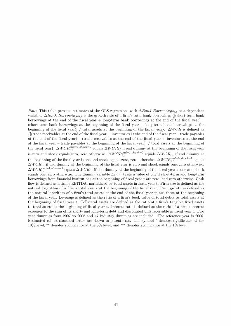
Note: This table presents estimates of the OLS regressions with ∆Bank Borrowingsi,t as a dependentvariable. ∆Bank Borrowingsi,t is the growth rate of a firm’s total bank borrowings {[(short-term bankborrowings at the end of the fiscal year + long-term bank borrowings at the end of the fiscal year) –(short-term bank borrowings at the beginning of the fiscal year + long-term bank borrowings at thebeginning of the fiscal year)] / total assets at the beginning of the fiscal year}. ∆WCR is defined as{[(trade receivables at the end of the fiscal year + inventories at the end of the fiscal year – trade payablesat the end of the fiscal year) – (trade receivables at the end of the fiscal year + inventories at the endof the fiscal year – trade payables at the beginning of the fiscal year)] / total assets at the beginning ofthe fiscal year}. ∆WCRend=0,shock=0

i,t equals ∆WCRi,t if end dummy at the beginning of the fiscal yearis zero and shock equals zero, zero otherwise. ∆WCRend=1,shock=0

i,t equals ∆WCRi,t if end dummy atthe beginning of the fiscal year is one and shock equals zero, zero otherwise. ∆WCRend=0,shock=1

i,t equals∆WCRi,t if end dummy at the beginning of the fiscal year is zero and shock equals one, zero otherwise.∆WCRend=1,shock=1

i,t equals ∆WCRi,t if end dummy at the beginning of the fiscal year is one and shockequals one, zero otherwise. The dummy variable Endi,t takes a value of one if short-term and long-termborrowings from financial institutions at the beginning of fiscal year t are zero, and zero otherwise. Cashflow is defined as a firm’s EBITDA, normalized by total assets in fiscal year t. Firm size is defined as thenatural logarithm of a firm’s total assets at the beginning of the fiscal year. Firm growth is defined asthe natural logarithm of a firm’s total assets at the end of the fiscal year minus those at the beginningof the fiscal year. Leverage is defined as the ratio of a firm’s book value of total debts to total assets atthe beginning of fiscal year t. Collateral assets are defined as the ratio of a firm’s tangible fixed assetsto total assets at the beginning of fiscal year t. Interest rate is defined as the ratio of a firm’s interestexpenses to the sum of its short- and long-term debt and discounted bills receivable in fiscal year t. Twoyear dummies from 2007 to 2008 and 47 industry dummies are included. The reference year is 2006.Estimated robust standard errors are shown in parentheses. The symbol ∗ denotes significance at the10% level, ∗∗ denotes significance at the 5% level, and ∗∗∗ denotes significance at the 1% level.

41

Table 11: Estimated Results for Regression of Interest Rate

(1) (2) (3)Dependent Variable Interest Rate Interest Rate Interest RateFirm Size All Medium Small

∆WCRend=0,shock=0i,t -0.0013 -0.0013 -0.0011

(0.002) (0.003) (0.004)

∆WCRend=1,shock=0i,t 0.0034 0.0026 0.0040

(0.002) (0.003) (0.004)

∆WCRend=0,shock=1i,t -0.0014 -0.0067∗∗ 0.0061

(0.003) (0.003) (0.006)

∆WCRend=1,shock=1i,t -0.0023 -0.0005 -0.0058

(0.003) (0.004) (0.006)End -0.0118∗∗∗ -0.0111∗∗∗ -0.0127∗∗∗

(0.000) (0.000) (0.000)Cash Flow 0.0023∗∗ -0.0004 0.0036∗∗

(0.001) (0.001) (0.002)Firm Size 0.0002∗∗∗ -0.0005∗∗∗ 0.0008∗∗∗

(0.000) (0.000) (0.000)Firm Growth 0.0011∗∗ 0.0012 0.0008

(0.001) (0.001) (0.001)Leverage 0.0092∗∗∗ 0.0098∗∗∗ 0.0080∗∗∗

(0.000) (0.000) (0.000)Collateral Assets 0.0011∗∗∗ 0.0026∗∗∗ -0.0002

(0.000) (0.000) (0.001)Year Dummy Yes Yes YesIndustrial Dummy Yes Yes YesObservations 29,864 18,999 10,865R-squared 0.221 0.208 0.246

Note: This table presents estimates of OLS regressions with Interest Ratei,t as a dependent variable.Interest Ratei,t is defined as the ratio of a firm’s interest expenses to the sum of its short- and long-termdebt and discounted bills receivable in fiscal year t. Other definitions of each variable are given in thenote for Table 10. Two year dummies from 2007 to 2008 and 47 industry dummies are included. Thereference year is 2006. Estimated robust standard errors are shown in parentheses. The symbol ∗ denotessignificance at the 10% level, ∗∗ denotes significance at the 5% level, and ∗∗∗ denotes significance at the1% level.

42

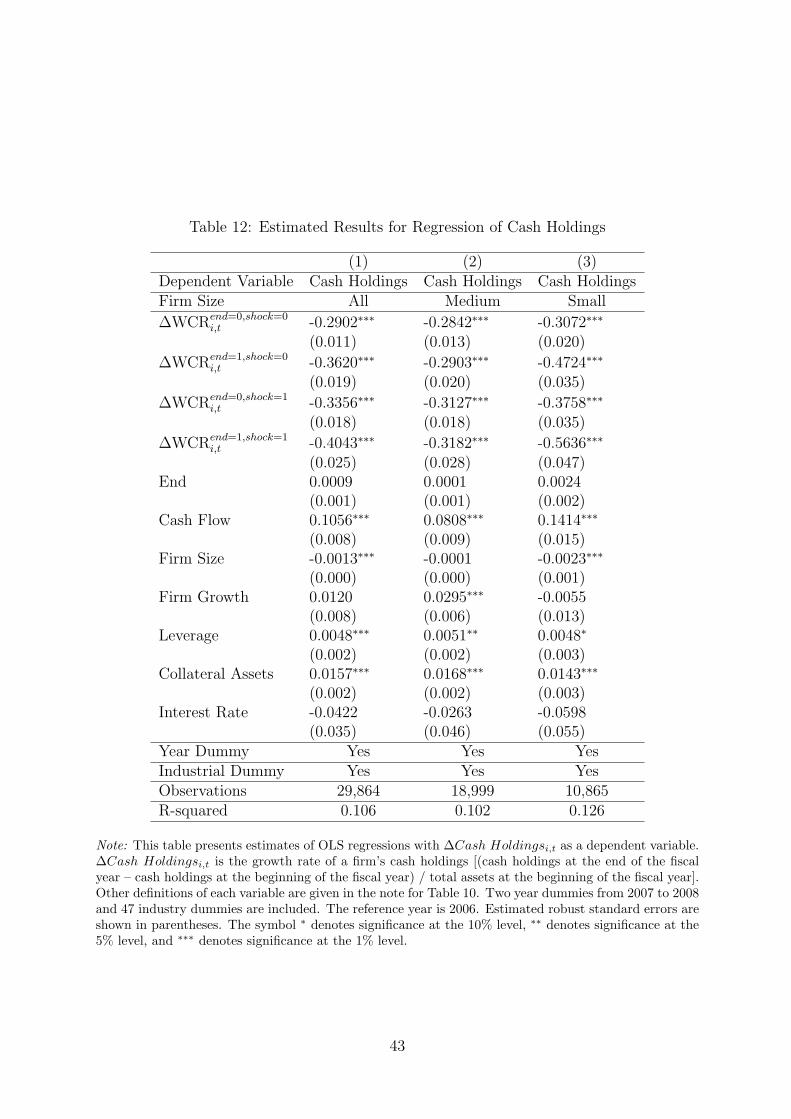
Table 12: Estimated Results for Regression of Cash Holdings

(1) (2) (3)Dependent Variable Cash Holdings Cash Holdings Cash HoldingsFirm Size All Medium Small

∆WCRend=0,shock=0i,t -0.2902∗∗∗ -0.2842∗∗∗ -0.3072∗∗∗

(0.011) (0.013) (0.020)

∆WCRend=1,shock=0i,t -0.3620∗∗∗ -0.2903∗∗∗ -0.4724∗∗∗

(0.019) (0.020) (0.035)

∆WCRend=0,shock=1i,t -0.3356∗∗∗ -0.3127∗∗∗ -0.3758∗∗∗

(0.018) (0.018) (0.035)

∆WCRend=1,shock=1i,t -0.4043∗∗∗ -0.3182∗∗∗ -0.5636∗∗∗

(0.025) (0.028) (0.047)End 0.0009 0.0001 0.0024

(0.001) (0.001) (0.002)Cash Flow 0.1056∗∗∗ 0.0808∗∗∗ 0.1414∗∗∗

(0.008) (0.009) (0.015)Firm Size -0.0013∗∗∗ -0.0001 -0.0023∗∗∗

(0.000) (0.000) (0.001)Firm Growth 0.0120 0.0295∗∗∗ -0.0055

(0.008) (0.006) (0.013)Leverage 0.0048∗∗∗ 0.0051∗∗ 0.0048∗

(0.002) (0.002) (0.003)Collateral Assets 0.0157∗∗∗ 0.0168∗∗∗ 0.0143∗∗∗

(0.002) (0.002) (0.003)Interest Rate -0.0422 -0.0263 -0.0598

(0.035) (0.046) (0.055)Year Dummy Yes Yes YesIndustrial Dummy Yes Yes YesObservations 29,864 18,999 10,865R-squared 0.106 0.102 0.126

Note: This table presents estimates of OLS regressions with ∆Cash Holdingsi,t as a dependent variable.∆Cash Holdingsi,t is the growth rate of a firm’s cash holdings [(cash holdings at the end of the fiscalyear – cash holdings at the beginning of the fiscal year) / total assets at the beginning of the fiscal year].Other definitions of each variable are given in the note for Table 10. Two year dummies from 2007 to 2008and 47 industry dummies are included. The reference year is 2006. Estimated robust standard errors areshown in parentheses. The symbol ∗ denotes significance at the 10% level, ∗∗ denotes significance at the5% level, and ∗∗∗ denotes significance at the 1% level.

43

Table 13: Estimated Results for Regression of Operating Incomes

(1) (2) (3)Dependent Variable Operating Operating Operating

Income Income IncomeFirm Size All Medium Small

End × Shock -0.0018 -0.0036 0.0006(0.002) (0.003) (0.004)

End 0.0005 0.0051∗∗∗ -0.0065∗∗∗

(0.001) (0.002) (0.002)Firm Size 0.0096∗∗∗ 0.0063∗∗∗ 0.0100∗∗∗

(0.000) (0.000) (0.001)Firm Growth 0.0724∗∗∗ 0.0797∗∗∗ 0.0611∗∗∗

(0.004) (0.005) (0.007)Leverage -0.0131∗∗∗ -0.0233∗∗∗ -0.0084∗∗∗

(0.002) (0.003) (0.003)Collateral Assets -0.0153∗∗∗ -0.0246∗∗∗ -0.0038

(0.002) (0.003) (0.003)Year Dummy (FY2007) -0.0003 0.0012 -0.0030

(0.001) (0.001) (0.002)Year Dummy (FY2008) -0.0097∗∗∗ -0.0090∗∗∗ -0.0103∗∗∗

(0.001) (0.001) (0.002)Industrial Dummy Yes Yes YesObservations 29,679 18,901 10,778R-squared 0.105 0.108 0.084

Note: This table presents estimates of OLS regressions with Firm Performancei,t as a dependentvariable. We use the operating income ratio, which is defined as the ratio of a firm’s operating incometo total assets in fiscal year t, as a proxy of firm performance. Other variable definitions are given in thenote for Table 10. Two year dummies from 2007 to 2008 and 47 industry dummies are included. Thereference year is 2006. Estimated robust standard errors are shown in parentheses. The symbol ∗ denotessignificance at the 10% level, ∗∗ denotes significance at the 5% level, and ∗∗∗ denotes significance at the1% level. The numbers are expressed in percentage terms.

44

Table 14: Median of Growth Rates of Total Bank Borrowings and Cash Holdings inFY2008, by Four Quantiles of Cash Holdings

Panel A: Total Borrowings∆WCR Over 0% - 2.5% 2.5% or more4 quantiles of End=0 End=1 Difference End=0 End=1 Differencecash holdings

1 -0.28 0.00 -0.28 1.00 0.00 1.00 ∗∗∗

2 0.00 0.00 0.00 2.16 0.00 2.16 ∗∗

3 -0.40 0.00 -0.40 ∗∗ 1.35 0.00 1.35 ∗∗

4 -0.45 0.00 -0.45 ∗∗∗ 0.18 0.00 0.18

Panel B: Cash Holdings∆WCR Over 0% - 2.5% 2.5% or more4 quantiles of End=0 End=1 Difference End=0 End=1 Differencecash holdings

1 0.04 0.00 0.04 0.01 0.00 0.012 -0.12 0.43 -0.55 -0.57 -1.77 1.19 ∗∗∗

3 -0.90 -0.74 -0.16 -2.24 -3.71 1.47 ∗∗

4 -1.42 -0.47 -0.95 ∗ -6.07 -6.24 0.17

Note: This table presents the median of growth rates of total bank borrowings and cash holdings. Growthrate of total bank borrowings is defined as [(total bank borrowings at the end of FY2008 – total bankborrowings at the beginning of FY2008) / total assets at the beginning of FY2008]. Growth rate of cashholdings is defined as [(cash holdings at the end of FY2008 – cash holdings at the beginning of FY2008)/ total assets at the beginning of FY2008]. ∆WCR is defined as WCR at the end of FY2008 – WCR atthe beginning of FY2008. The numbers are expressed in percentage terms. Each row is divided into fourquantiles of cash holdings normalized by total assets at the beginning of FY2008. The symbol ∗ denotessignificance at the 10% level, ∗∗ denotes significance at the 5% level, and ∗∗∗ denotes significance at the1% level.

45

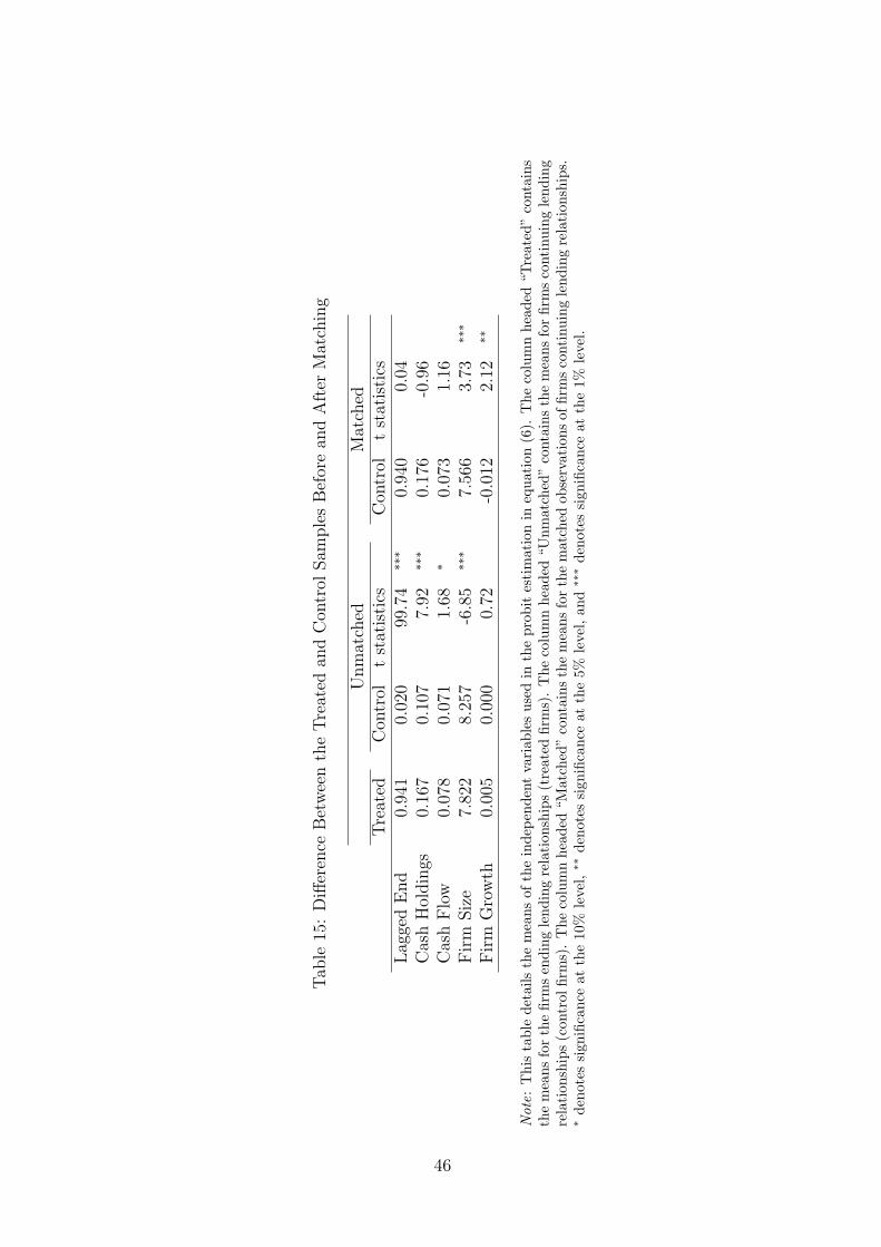
Tab

le15

:D

iffer

ence

Bet

wee

nth

eTre

ated

and

Con

trol

Sam

ple

sB

efor

ean

dA

fter

Mat

chin

g

Unm

atch

edM

atch

edTre

ated

Con

trol

tst

atis

tics

Con

trol

tst

atis

tics

Lag

ged

End

0.94

10.

020

99.7

4∗∗

∗0.

940

0.04

Cas

hH

oldin

gs0.

167

0.10

77.

92∗∗

∗0.

176

-0.9

6C

ash

Flo

w0.

078

0.07

11.

68∗

0.07

31.

16Fir

mSiz

e7.

822

8.25

7-6

.85

∗∗∗

7.56

63.

73∗∗

∗

Fir

mG

row

th0.

005

0.00

00.

72-0

.012

2.12

∗∗

Not

e:T

his

tabl

ede

tails

the

mea

nsof

the

inde

pend

ent

vari

able

sus

edin

the

prob

ites

tim

atio

nin

equa

tion

(6).

The

colu

mn

head

ed“T

reat

ed”

cont

ains

the

mea

nsfo

rth

efir

ms

endi

ngle

ndin

gre

lati

onsh

ips

(tre

ated

firm

s).

The

colu

mn

head

ed“U

nmat

ched

”co

ntai

nsth

em

eans

for

firm

sco

ntin

uing

lend

ing

rela

tion

ship

s(c

ontr

olfir

ms)

.T

heco

lum

nhe

aded

“Mat

ched

”co

ntai

nsth

em

eans

for

the

mat

ched

obse

rvat

ions

offir

ms

cont

inui

ngle

ndin

gre

lati

onsh

ips.

∗de

note

ssi

gnifi

canc

eat

the

10%

leve

l,∗∗

deno

tes

sign

ifica

nce

atth

e5%

leve

l,an

d∗∗

∗de

note

ssi

gnifi

canc

eat

the

1%le

vel.

46

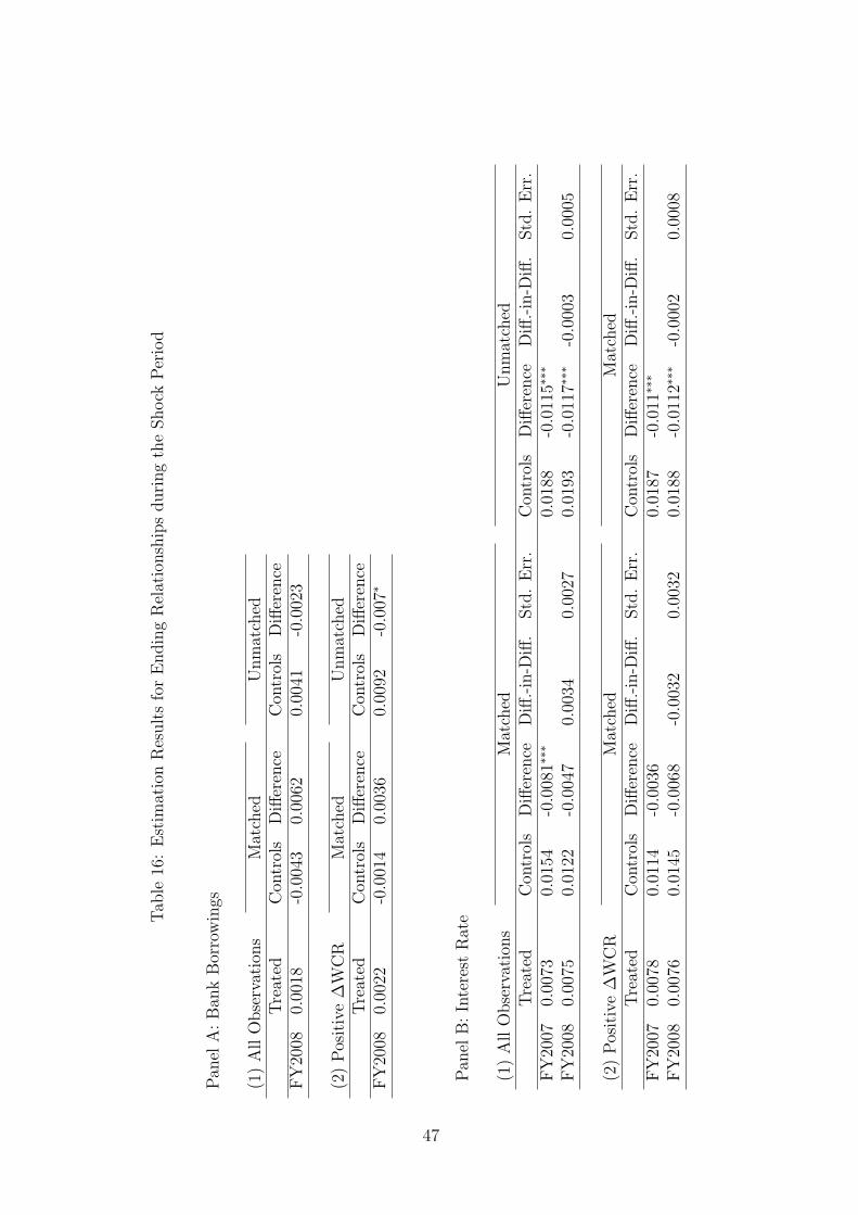
Tab

le16

:E

stim

atio

nR

esult

sfo

rE

ndin

gR

elat

ionsh

ips

duri

ng

the

Shock

Per

iod

Pan

elA

:B

ank

Bor

row

ings

(1)

All

Obse

rvat

ions

Mat

ched

Unm

atch

edTre

ated

Con

trol

sD

iffer

ence

Con

trol

sD

iffer

ence

FY

2008

0.00

18-0

.004

30.

0062

0.00

41-0

.002

3

(2)

Pos

itiv

e∆

WC

RM

atch

edU

nm

atch

edTre

ated

Con

trol

sD

iffer

ence

Con

trol

sD

iffer

ence

FY

2008

0.00

22-0

.001

40.

0036

0.00

92-0

.007

∗

Pan

elB

:In

tere

stR

ate

(1)

All

Obse

rvat

ions

Mat

ched

Unm

atch

edTre

ated

Con

trol

sD

iffer

ence

Diff

.-in

-Diff

.Std

.E

rr.

Con

trol

sD

iffer

ence

Diff

.-in

-Diff

.Std

.E

rr.

FY

2007

0.00

730.

0154

-0.0

081∗

∗∗0.

0188

-0.0

115∗

∗∗

FY

2008

0.00

750.

0122

-0.0

047

0.00

340.

0027

0.01

93-0

.011

7∗∗∗

-0.0

003

0.00

05

(2)

Pos

itiv

e∆

WC

RM

atch

edM

atch

edTre

ated

Con

trol

sD

iffer

ence

Diff

.-in

-Diff

.Std

.E

rr.

Con

trol

sD

iffer

ence

Diff

.-in

-Diff

.Std

.E

rr.

FY

2007

0.00

780.

0114

-0.0

036

0.01

87-0

.011

∗∗∗

FY

2008

0.00

760.

0145

-0.0

068

-0.0

032

0.00

320.

0188

-0.0

112∗

∗∗-0

.000

20.

0008

47

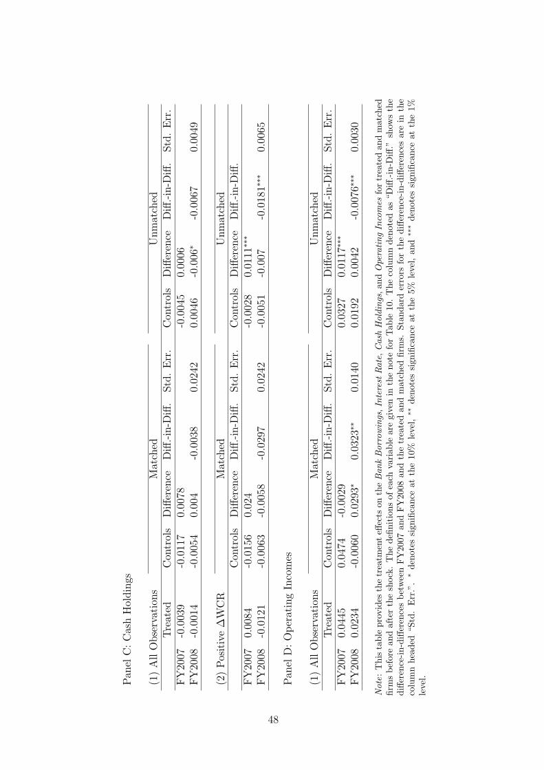
Pan

elC

:C

ash

Hol

din

gs

(1)

All

Obse

rvat

ions

Mat

ched

Unm

atch

edTre

ated

Con

trol

sD

iffer

ence

Diff

.-in

-Diff

.Std

.E

rr.

Con

trol

sD

iffer

ence

Diff

.-in

-Diff

.Std

.E

rr.

FY

2007

-0.0

039

-0.0

117

0.00

78-0

.004

50.

0006

FY

2008

-0.0

014

-0.0

054

0.00

4-0

.003

80.

0242

0.00

46-0

.006

∗-0

.006

70.

0049

(2)

Pos

itiv

e∆

WC

RM

atch

edU

nm

atch

edC

ontr

ols

Diff

eren

ceD

iff.-in

-Diff

.Std

.E

rr.

Con

trol

sD

iffer

ence

Diff

.-in

-Diff

.FY

2007

0.00

84-0

.015

60.

024

-0.0

028

0.01

11∗∗

∗

FY

2008

-0.0

121

-0.0

063

-0.0

058

-0.0

297

0.02

42-0

.005

1-0

.007

-0.0

181∗

∗∗0.

0065

Pan

elD

:O

per

atin

gIn

com

es

(1)

All

Obse

rvat

ions

Mat

ched

Unm

atch

edTre

ated

Con

trol

sD

iffer

ence

Diff

.-in

-Diff

.Std

.E

rr.

Con

trol

sD

iffer

ence

Diff

.-in

-Diff

.Std

.E

rr.

FY

2007

0.04

450.

0474

-0.0

029

0.03

270.

0117

∗∗∗

FY

2008

0.02

34-0

.006

00.

0293

∗0.

0323

∗∗0.

0140

0.01

920.

0042

-0.0

076∗

∗∗0.

0030

Not

e:T

his

tabl

epr

ovid

esth

etr

eatm

ent

effec

tson

the

Ban

kBor

rowin

gs,I

nter

estRat

e,C

ash

Hol

ding

s,an

dO

pera

ting

Inco

mes

for

trea

ted

and

mat

ched

firm

sbe

fore

and

afte

rth

esh

ock.

The

defin

itio

nsof

each

vari

able

are

give

nin

the

note

for

Tab

le10

.T

heco

lum

nde

note

das

“Diff

.-in

-Diff

.”sh

ows

the

diffe

renc

e-in

-diff

eren

ces

betw

een

FY

2007

and

FY

2008

and

the

trea

ted

and

mat

ched

firm

s.St

anda

rder

rors

for

the

diffe

renc

e-in

-diff

eren

ces

are

inth

eco

lum

nhe

aded

“Std

.E

rr.”

.∗

deno

tes

sign

ifica

nce

atth

e10

%le

vel,

∗∗de

note

ssi

gnifi

canc

eat

the

5%le

vel,

and

∗∗∗

deno

tes

sign

ifica

nce

atth

e1%

leve

l.

48