NASA Technical Memorandum 78666

1178-200714(NASA-TM-78666) ONSET OF: CONIENSATION EFFECTS WITH A,NACA 0012-:64 AIRFOIL TESTED IN THE LANGLEY-O. 3-METER; CEXOGENIC TUNNEL (NASK] 84 p HC' A05/MF,'AO1 CSCL,01A Unclas

G3/02 11898

ONSET OF CONDENSATION EFFECTS WITH A NACA 0012-64 AIRFOIL TESTED IN THE LANGLEY 0.3-METER CRYOGENIC TUNNEL

Robert M. Hall

March 1978

NJASA National Aeronautics and -1 Space Administration Langley Research Center

Hampton, Virginia 23665 ...

https://ntrs.nasa.gov/search.jsp?R=19780012131 2020-03-20T09:45:22+00:00Z

SUMMARY

A 0.137-m NACA oo2-64 airfoil has been tested in the Langley 0.3-m

transonic cryogenic tunnel at free-stream Mach numbers of 0.75, 0.85, and 0.95

over a total pressure range from 1.2 to 5.0 atmospheres. The onset of conden­

sation effects were found to correlate more with the amount of supercooling

in the free-stream than it did with the supercooling in the region of maximum

local Mach number over the airfoil. Effects in the pressure distribution over

the airfoil 'were generally seen to appear over its entire length at nearlythe

same total temperature. Both observations suggest the possibility of hetero­

geneous nucleation occurring in the free-stream. Comparisons of the present

onset results are made to calculations by Sivier and data by Goglia. The

potential operational benefits of the supercooling realized are presented

in terms of increased Reynolds number capability at a given tunnel total

pressure, reduced drive fan power if Reynolds number is held constant, and

reduced liquid nitrogen consumption if Reynolds number is again constant.

Depending on total pressure and free-stream Mach number, these three benefits

are found to respectively vary from 7 to 19%, 11 to 25%, and 9 to 20%.

Appendices are included which give details of the data analysis procedure

and of the error bar calculation for the differences in pressure distributions.

ORIGINAL rAGE 1S

OF POOR QUALM

INTRODUCTION

Cryogenic wind tunnels should be operated at the lowest possible total

temperatures in order to maximize the advantages of cryogenic operation, such

as increased Reynolds number and reduced operating costs. However, minimum

operating temperatures are limited by low temperature effects on the flow,

which can be the result of real-gas behavior of the test-gas. Either the equa­

tion of state of the test-gas changes in such a manner that the gas does not

properly simulate the nearly ideal-gas behavior of air encountered in flight,

or the gas begins to condense and consequently does-not properly simulate the

nearly ideal-gas behavior of air. Analyzing the nitrogen test-gas over the

operating ranges of existing and proposed transonic cryogenic wind tunnels,

Adcock reported in reference 1 that low temperature nitrogen gas approximates

an ideal-gas during flow simulations for total pressures under l0 atmospheres

and for Mach numbers up to 2. Consequently, the lower temperature boundary

appears to be determined by condensation of the nitrogen test-gas. The

boundary is important from an operational viewpoint because it determines, on

one hand, the maximum Reynolds number capability for a fixed tunnel total

pressure and, on the other hand, the most economical total temperature and

pressure to operate the tunnel for a fixed test Reynolds number.

Condensation not only has an important role in determining the operational

envelope for transonic cryogenic tunnels but has a similar role for supersonic

and hypersonic tunnels. Wegener and Mack in reference 2 give a summary of

historical events leading to, and the results from, many of the condensation

investigations in supersonic and hypersonic tunnels.

3

investigation employs a pressure-instrumentedThe present condensation

NACA 0012-6h airfoil mounted in the Langley 0.3-m transonic cryogenic tunnel.

Changes in the pressure distribution over the airfoil have been used to detect

as changes in pressurethe onset of condensation effects in a similar fashion

were used in references 2 to 6 to detectdistributions in divergent nozzles

the onset of condensation effects at supersonic and hypersonic speeds. The

free-stream Mach numbers of 0.75, 0.85, and 0.95airfoil has been tested at

over a total pressure range of 1.2 to 5.0 atmospheres in order to determine the

total temperature at which condensation influences the flow about the airfoil

free-stream Mach number.as a function of total pressure and

pALISOF p1OOR QUALLTYORIGINAL 'PAGE T

SYMBOLS

a sound, speed

c airfoil chord, 0.137-m p - pw

C pressure coefficient, p ACp difference in Cp defined by equation (A6)

p pressure, atm

Ap pressure instrumentation accuracy

q dynamic pressure

R Reynolds number

T temperature, K

AT supercooling defined by equation (1)

x linear dimension along airfoil chord line

11 viscosity

p density

o standard deviation

Subscripts

e conditions at onset of condensation effects

L local conditions

s conditions at intersection of isentrope and vapor pressure curve

t total conditions

wfree-stream conditions

5

MINIMUM OPERATING TEMPERATURES I

The maximum Reynolds number capability and the operating costs of a

cryogenic wind tunnel are both affected by the minimum operating temperatures

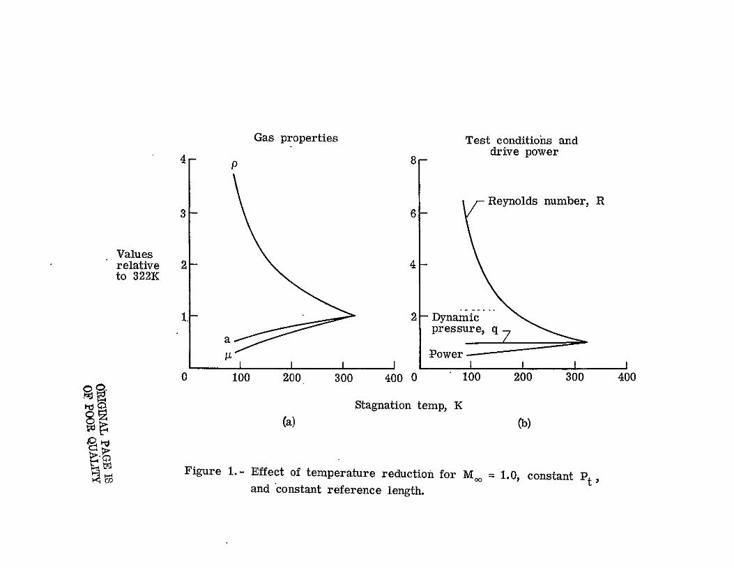
of the tunnel. The reasons for this can be understood by reviewin the effects

of changing tunnel temperature upon the test gas, which are shown in fig­

ures l(a) and l(b). In figure l(a) the behavior of the gas properties relative

to their ambient temperature values can be seen. The density, p, increases

while the viscosity, 1i, and the speed of sound, a, decrease as the total

temperature, Tt, decreases for a fixed value of tunnel total pressure, Pt.

As shown in figure l(b), the behavior of the gas properties as Tt decreases

leads to a dramatic increase in unit Reynolds number, R, a decrease in drive

power required, and no change in dynamic pressure, q. Consequently, it is

desirable to operate the tunnel as cold as is possible in order to'maximize R

and reduce drive power. Just how low in temperature the tunnel can be operated

is determined by the onset of condensation effects.

A conservative first guess for the minimum operating temperature is to

operate at temperatures which avoid any possibility of saturation occurring

anywhere over the model. Since the lowest static temperature over a model

occurs at the point of maximum local Mach number, ML , and Pt can bet max

chosen to keep the local static values of p, T just on the vapor phase side

of the vapor pressure curve for nitrogen. However, it has been found from tests

in the Langley 0.3-m transonic cryogenic tunnel and in other facilities that

condensation effects tend to be delayed to some lower temperature.

The delay in condensation onset past the vapor-pressure curve is due to

an energy barrier blocking stable liquid droplet formation - that is, blocking

self-nucleation of the test gas. Thus there will normally be a delay in

oRIGP1L pAGI 3

6 O pOO

droplet formation and growth, and consequently in effects, unless some catalyst

is available to speed the process. (More details of the various condensation

processes will be given in the section Implications of the Data.) The delay

in condensation can be quantitatively measured by the supercooling at onset of

effects, AT, which is defined as

AT = T - T Wi)

where T is the static temperature where the isentrope crosses the vapor

pressure curve and T is the static temperature along the isentrope wheree

effects are first seen.

If supercooling does occur then there are two wind tunnel operational

benefits that result. First of all, for a given.tunnel Pt the maximum R

capability is .increasedbecause at the lower temperature the unit is greater.R

as shown in figure l(b). This benefit would not only increase the maximum R

capability of a tunnel, but would also increase the R obtainable for a model

that may be q limited since q is proportional to Pt for a given M,.

Secondly, if maximum R capability is not important, then supercooling can be

used to reduce operating costs when operating at a fixed R. Operating at a

lower Tt than needed to avoid saturation permits a decrease in Pt for a

given value of R. Since drive fan power is proportional to pt and decreases

with decreasing Tt, both changes reduce the required drive power. Since

normally over 99% of the injected liquid nitrogen is used to absorb the heat

generated by the drive fan once the tunnel has been cooled, a reduction in

drive fan power leads to a reduction in the amount of injected liquid nitrogen.

7

Both reductions decrease direct operating costs, which are split with about

90% going to the injected liquid nitrogen and only 10% going to power the

drive fan. Specific details of drive power required and operating costs are

given in references 7 and 8.

EXPERETMAL APPARATUS

Tunnel

The Langley 0.3-m transonic cryogenic tunnel is a continuous flow, fan­

driven tunnel, which uses nitrogen as a test gas and is cooled by injecting

liquid nitrogen directly into the stream. Variation of the rate of liquid

nitrogen injection provides a total temperature range from nearly 77 to 350 K,

while the total pressure can be varied from 1.2 to 5.0 atm. The combined low

temperature and high pressure can produce a Reynolds number of over 330 million/m

(100 million/ft). Some of the design features and operational characteristics

of the 0.3-m tunnel have been reported by Kilgore in reference 9, and a sketch

of the tunnel is shown in figure 2.

The liquid nitrogen used to cool down the tunnel and absorb the heat of

the drive fan was injected into the tunnel through a series of eleven nozzles

arranged on three different struts, or spray bars, at the three injection

stations shown in figure 2. Full details of this arrangement are included in

reference 9. However, for one of the tests during the present investigation

(details to be mentioned in RESULTS AND DISCUSSION), the spray bar system was

removed and injection was carried out by injecting through just four nozzles

at injection station 1. This change, of course, necessitated larger liquid

flow rates per nozzle.

Airfoil and Installation

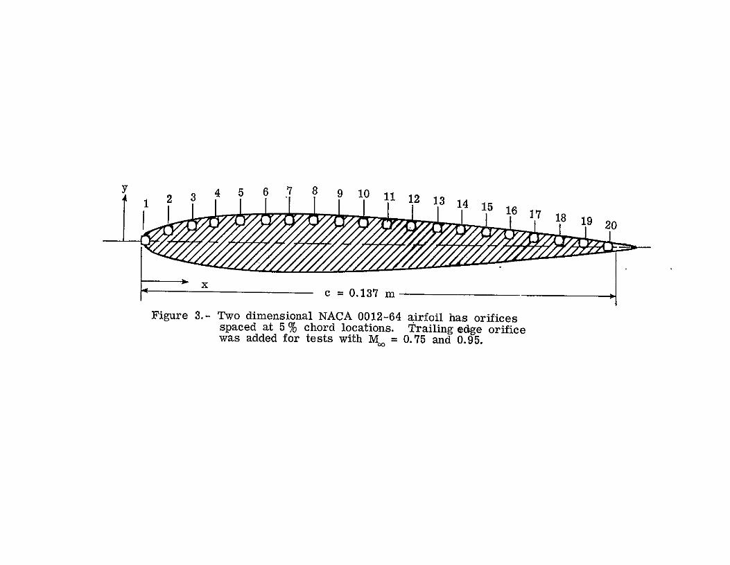
A 0.137-m NACA 0012-64 airfoil was used for these tests. Starting at the

leading edge, the airfoil had 20 pressure orifices spaced at 5% chord intervals

on both.the top and bottom surfaces. For the tests at M. of 0.75 and 0.95,

a rearward-facing orifice was added to the trailing edge of the airfoil. The

9

airfoil was installed between flats in the octagonal test section, with the

leading edge 0.62-m from the beginning of the test section. The angle of

attack of the airfoil was zero for all tests. A sketch of the airfoil is

given in figure 3.

The pressure distributions over the airfoil may be influenced by wall

interference effects because of the relatively large chord of the airfoil

compared to the size of the test section. However, wall interference should

not have an effect on the occurrence of condensation.

Data Acquisition and Error Discussion

The tunnel parameters were first recorded and then a differential pressure

transducer was used in a scanning valve system to step through and record the

pressures around the airfoil. The time to acquire all of the data for a

complete pressure distribution was 50 seconds.

The uncertainty in the pressure transducer measurements was less than 0.5 percent

of full scale, which was the magnitude specified by the manufacturer. In fact, the scatte

in the pressure transducer data was observed to be less than the stated value by more

than a factor of 10. For the transducer used in the tests at M = 0.75 and

0.95, the uncertainty was on the order of 0.0004 atm. For the transducer used in

the test at M = 0.85, the uncertainty was about 0.0002 atm. There was no

Significant error introduced by either the signal conditioning or data acquisition

systems. However, during the 50-second acquisition period, the tunnel conditions

were observed to fluctuate by the following amounts: M, ±.003; Tt, ±0.5K; and

p', approximately ±0.005 atm. A development of the uncertainty in C due to the

above fluctuations is contained in appendix B.

10

TESTS,

Data Sampled

To determine the total temperature at which effects do occur and to inves­

tigate the influence of total pressure and free-stream Mach number on the onset

of condensation effects, the airfoil was tested at- free-stream Mack numbers of

0.75, 0.85, and 0.95 over a total pressure range of 1.2 to 5.0 atm. For each

of the three values of M,, test envelopes were drawn which covered those

tunnel pt and Tt ranges that were of interest and that were obtainable in

the 0.3-m tunnel.

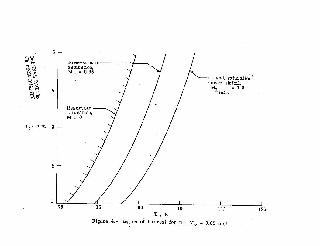
The test envelopes were bounded in pt by the 1.2 to 5.0 atm pressure

limits of the tunnel and were bounded in Tt by total temperatures corre­

sponding to saturated flow at ML and those corresponding to saturation

in the reservoir section. Figure 4 shows the M = 0.85 test envelope as an

example. Total con&itions which fall lower in Tt than the reservoir

saturation line are unobtainable since the injected liquid nitrogen used for cooling would never evaporate when Tt is below the vapor pressure curve and, consequently, furtt

cooling can not occur. Total temperatures above those along the line of local

saturation offer no possibility of condensation in a pure nitrogen test-gas so

they are used in this study only as a way of obtaining unaffected comparison

points. The locus of tunnel Pt and Tt which just allow saturation when

the flow is accelerated to M. is also given in figure 4.

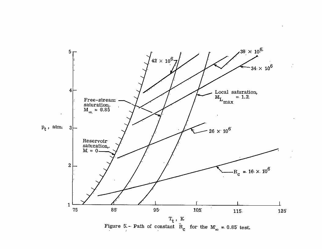
To explore each of the regions of interest in the Pt and Tt plane,

paths of constant Rc and M were used to traverse the region of interest.

Since along each of the paths both M. and were held constant; systematicRc

deviation in pressure coefficients at any x/c position over the airfoil was

11

taken to be the result of condensation effects. The paths of constant RC

and 14 are shown for the M = 0.85 test in figure '5. The Rc along each

path yaried from 16 million at the low pressure traverse to 42 million at the

Pgh pressure traverse. Along these 5 paths, ,atotal of 201 pressure distri­

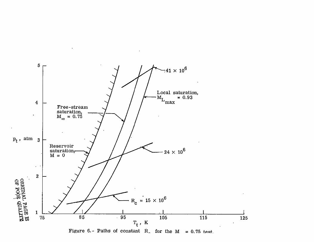
utions xere recorded and analyzed. Similar envelopes were drawn and

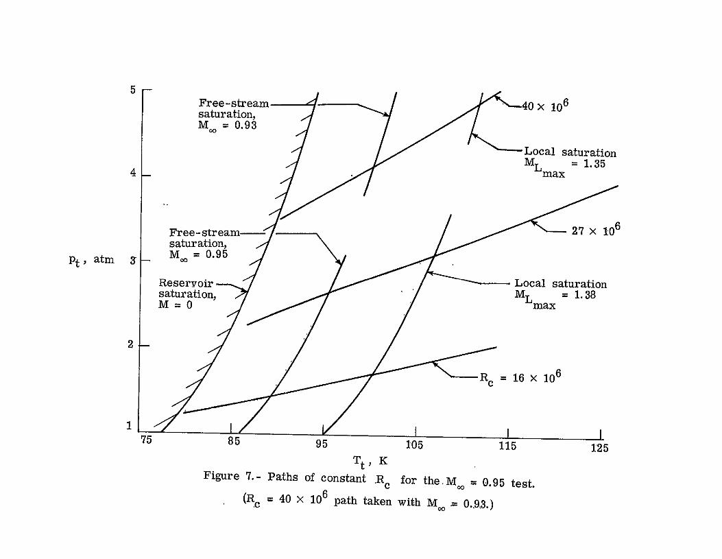
investigated for M = 0.75 and M = 0.95 except that only 3 paths of

constant R and M were used in these cases. These envelopes are shown in

figres ,6 and 7. During the investigation of the high pressure path for the

M = 0.95 test, a fan drive power limit was encountered so M was reduced

from 0.95 to 0.93 for that path alone.

Data Analysis

In order to determine the Pt and at which the onset of condensationTt

effects occurs along a constant M and Rc path, a special data analysis

procedure was developed. The main Qbjective of the data analysis procedure was

to be able to correct values of C on an orifice-by-orifice basis in casesp

where the pressure distribution over the airfoil was taken at a slightly

different M than desired. With such a correction, data along the path that

normally would have had to be disregarded due to small differences in M could

be utilized. Having more data available made it easier to detect the total

temperature at which differences in Cp, ACp, begin to occur because of the

effects of condensation.

Once the values of total temperature for the onset of effects at each

orifice had been determined, a graph of orifice onset total temperature as a

function of x/c could be drawn for the path of constant M. and Rc In.

this manner, an appropriate onset total temperature could be chosen for the

airfoil as a whole. Further details of the data analysis procedure are

presented in appendix A.

12

RESULTS AND DISCUSSION

Data Presentation and Comments

The data, taken and analyzed as discussed in the previous section, will be

summarized by a series of figures for each value of M - 0.75, 0:85, and 0.95­

covered in this study. Each series will include average, condensation-free

pressure distributions for each path of constant Rc graphs of orifice onset

Tt as a function of x/c for each path; and a summary plot for each K

showing the onset conditions for each path in a Tt versus Pt plane. The

results for all of the M will then be grouped together assuming either ML

or M is the important Mach number parameter.

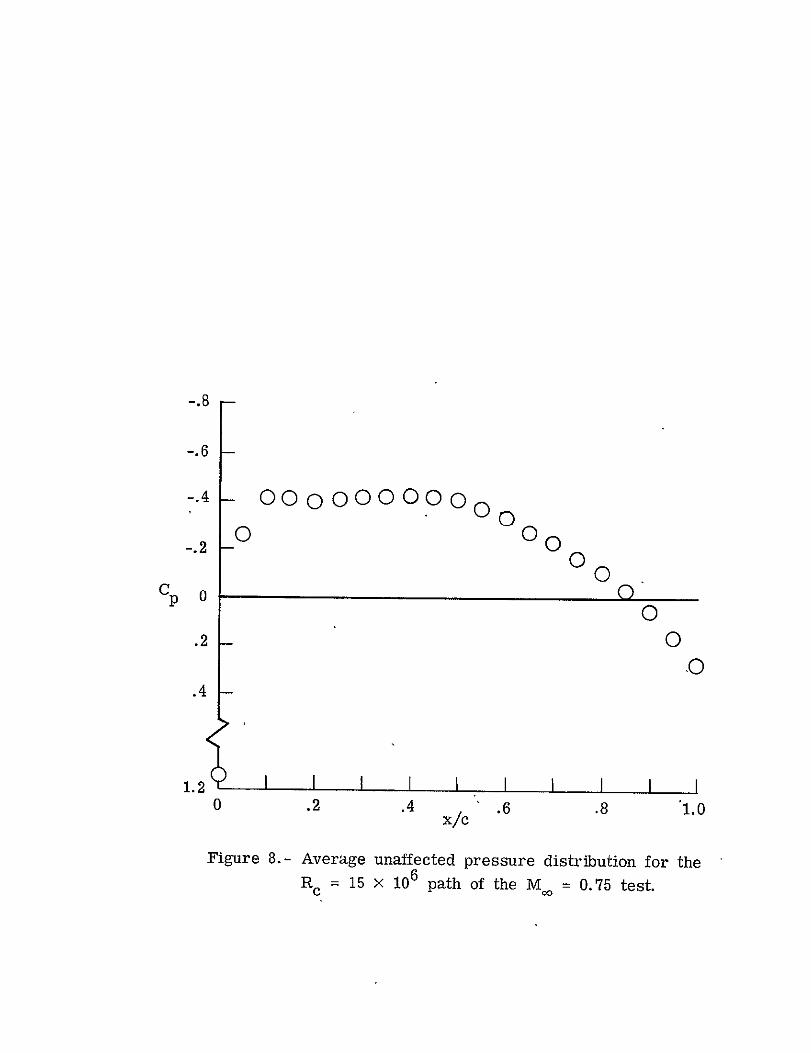
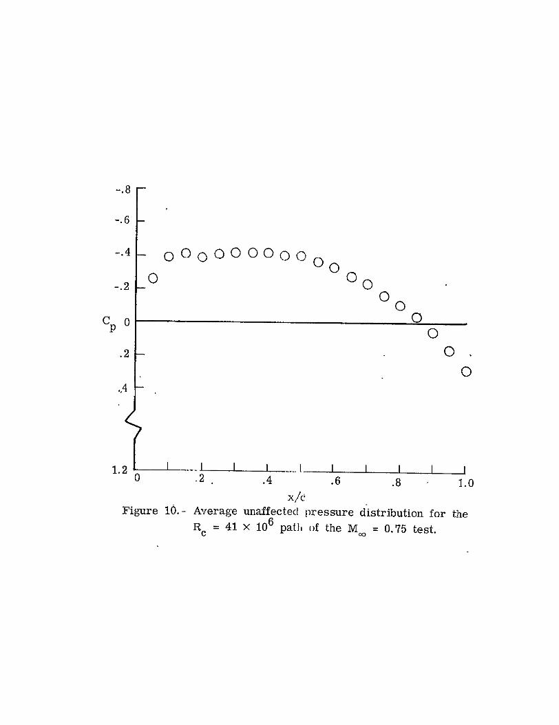
The first test described is the M = 0.75 test. The average pressure

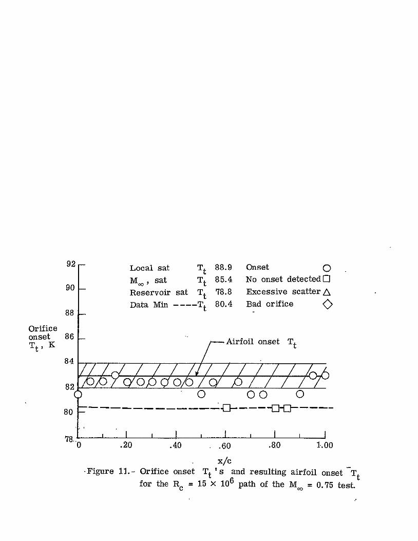
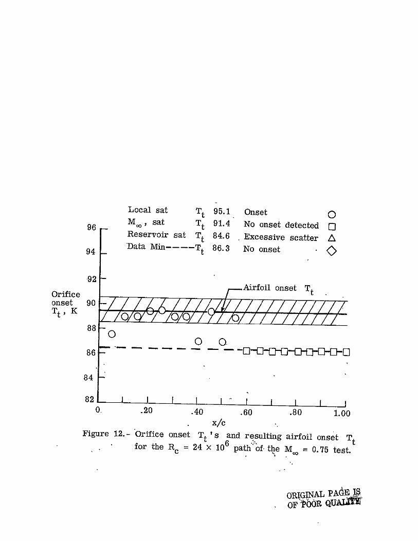
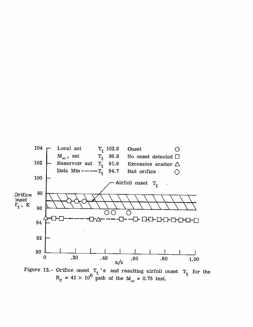
distributions are shorwn in figures 8, 9, and 10, and the orifice onset vs.Tt

x/c graphs are shown in figures 11, 12, and 13. Four different symbols are

plotted in the orifice onset graphs corresponding to four different situations.

When normal orifice onset is detected, a circle is plotted at the appropriate

x/c, Tt location. When no orifice,onset is detected, a square is plotted at

the minimum Tt at which data was taken. When excessive scatter obscures any

trends, a triangle is plotted at the minimum T When an orifice pressure

tube developed a leak, a diamond is plotted at the minimum T It is

interesting to note in figures 11, 12, and 13 that the airfoil appears to be

most sensitive to condensation effects in the 15-25% chord location, as is

seen most clearly in figures 12 and 13. There does not seem to be any greater

sensitivity to condensation over the rearward portion of the airfoil, which

seems to downplay the importance of any condensate growth over the airfoil

itself. The summary plot of onset conditions is shown in figure 14.

13

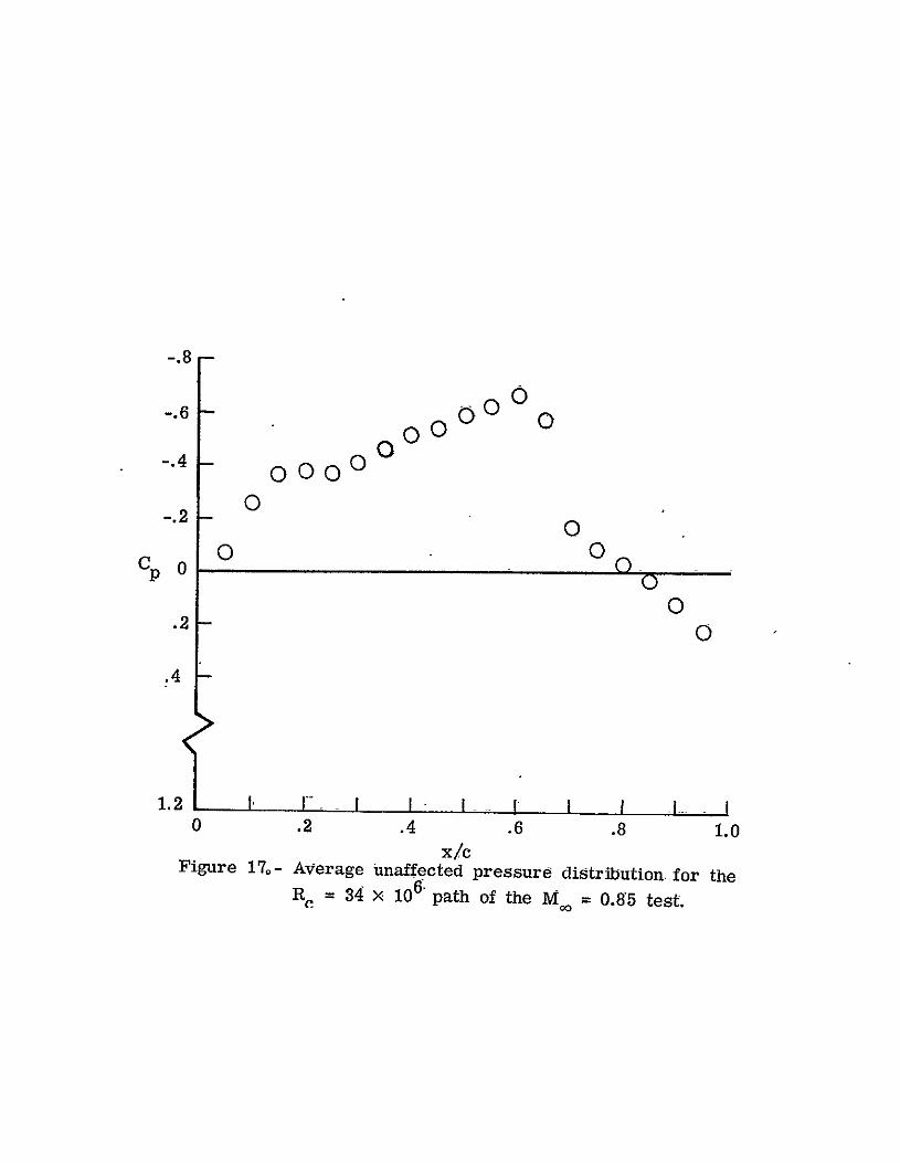
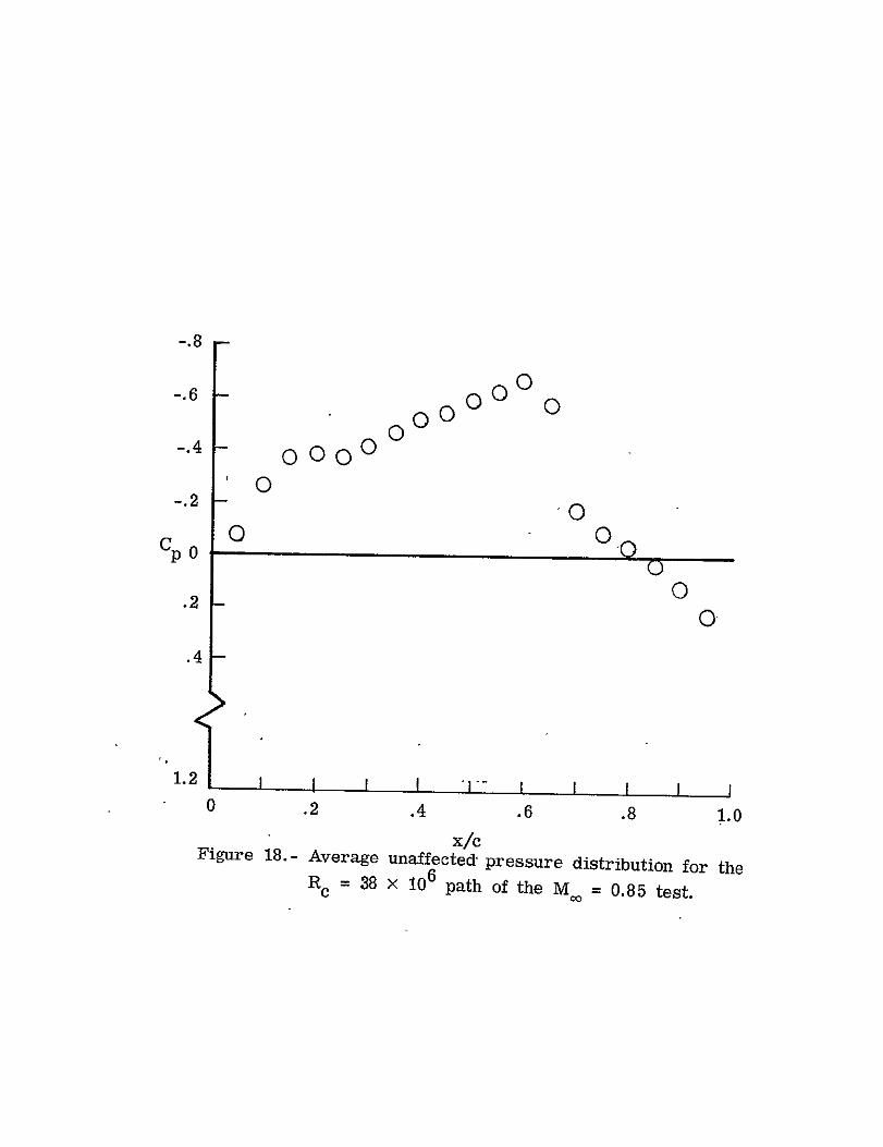
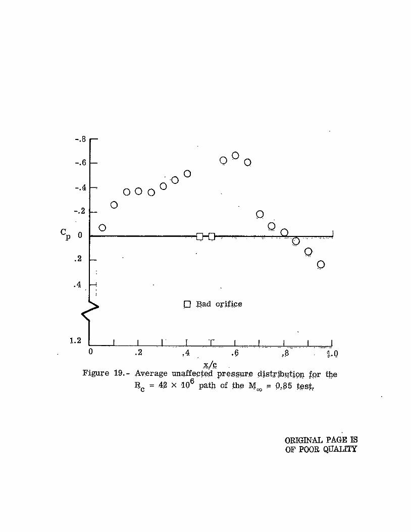
The pressure distributions for the 5 lines of constant Rc for the

M = 0.85 test are shown in figures 15, 16, 17, 18, and 19 and exhibit a

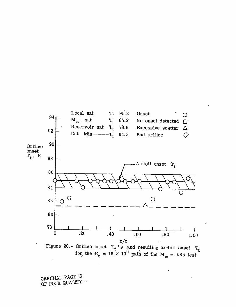
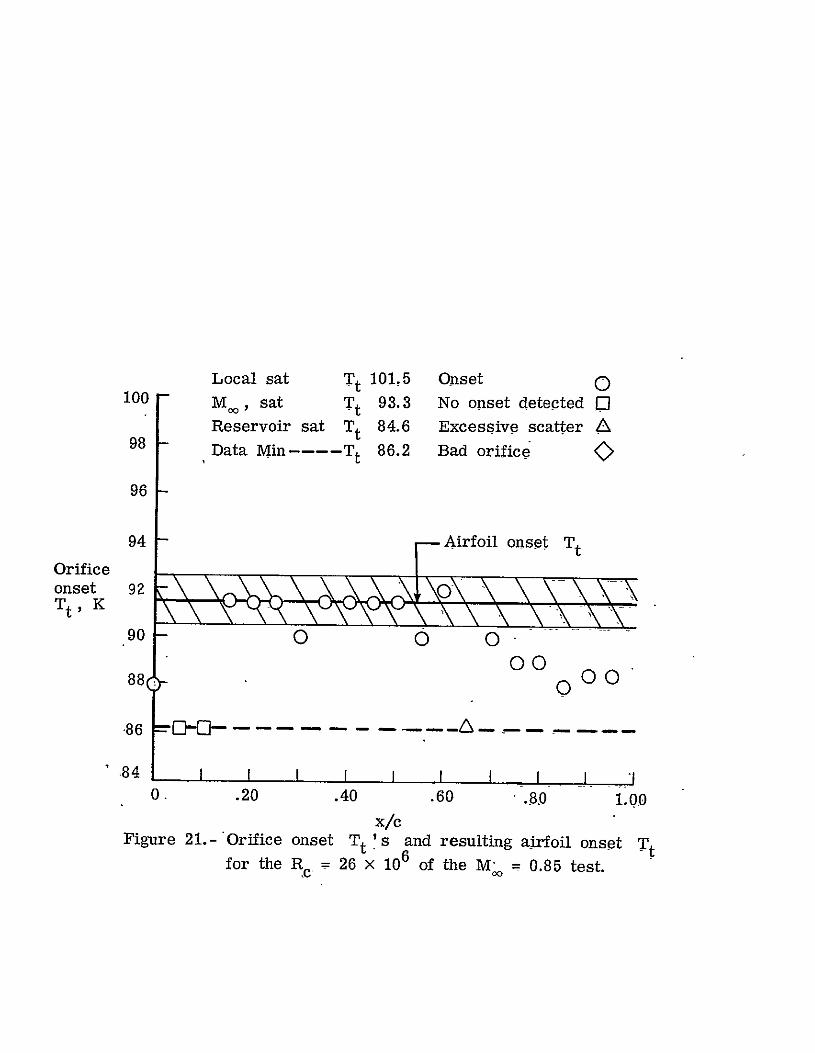
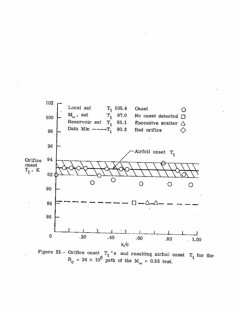
recompression shock at the 0.65 x/c location. The graphs showing orifice

onset Tt as a function of x/c are shown in figures 20, 21, 22, 23, and 24.

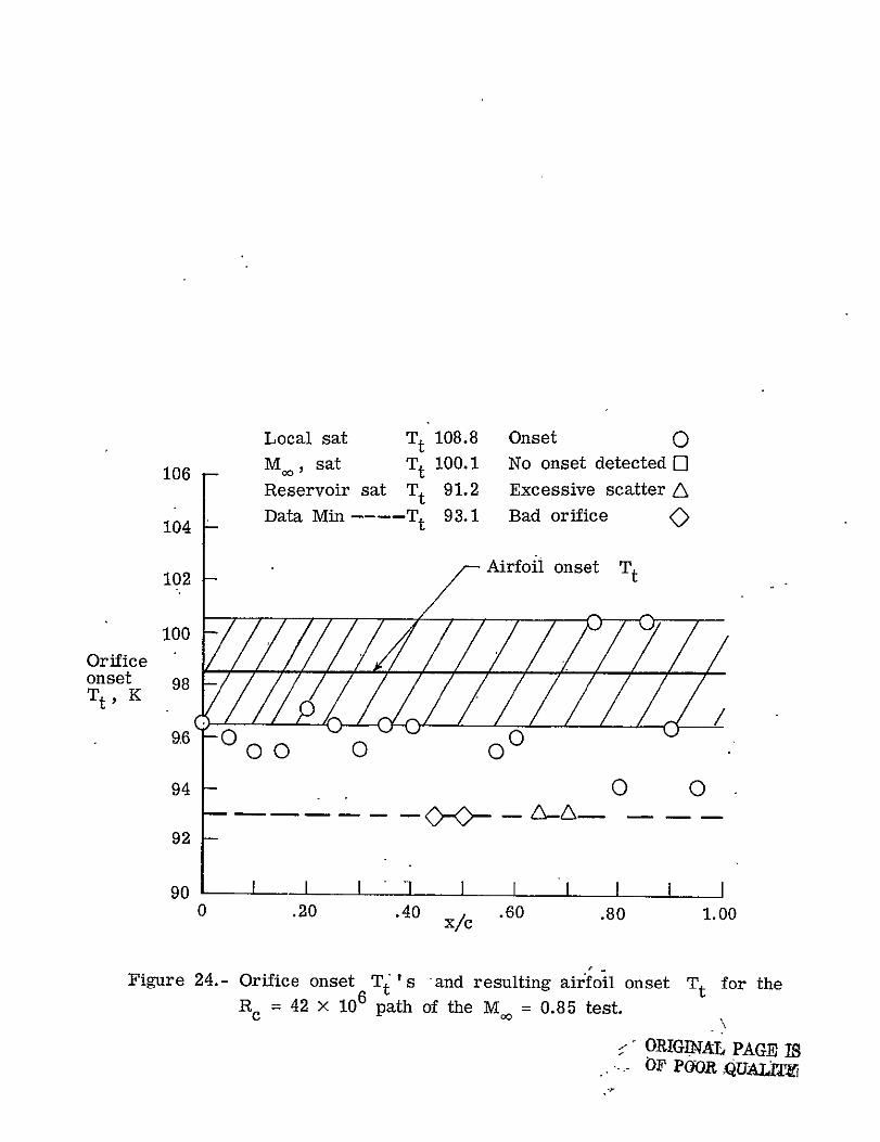
With the possible exception of figure 24, it appears that effects

occur at about the same Tt over the length of the airfoil. That is, there is

not an obvious sensitivity to condensation effects behind the shock, or even

right before the shock in the region of high local Mach number. Along the.

Ra = 42 million path as shown in figure 24, there does appear to be possibl

sensitivity behind the shock location. At x/c values of 0.75 and 0.85 the

onset value of Tt appeared to be 100.5 K, which is above the trend of effects

occurring at about 96 or 96.5 K for the majority of orifices. While the onset

Tt of 100.5 K may be correct, there is scatter in the ACp vs. Tt graphs that

were combined to form figure 24. Because of the uncertainties involved and

because of the lack of agreement between orifice onset Tt's behind the shock

location at x/c = 0.65 in figure 24, the airfoil onset Tt was chosen to be

98.5 K with a possible error bar extending from 96.5 to 100.5 K. The summary

plot of onset conditions for the M = 0.85 test is given in figure 25.

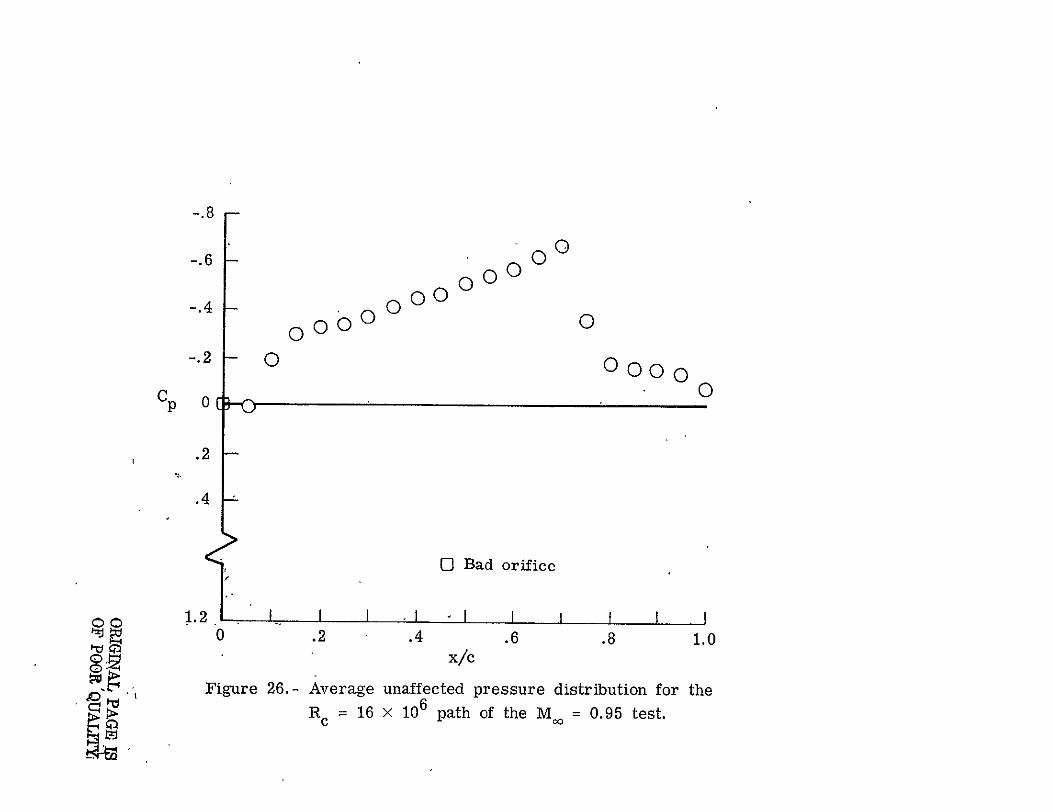
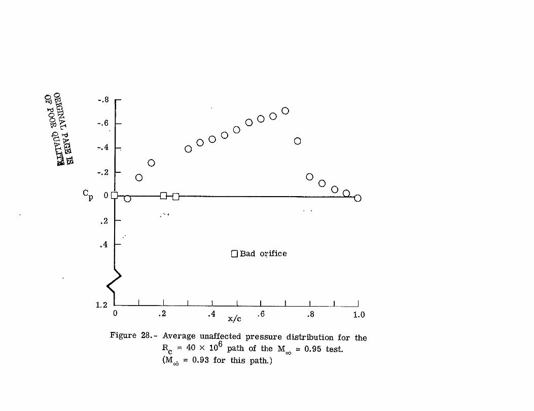
The last test condition was that of M = 0.95. As mentioned under the

section Data Sampled, the high pressure path at R- 40 million was testedc

at M = 0.93 instead of 0.95, so there is a M difference between the first

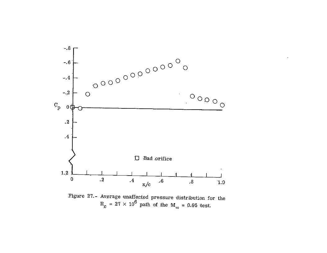
2 paths and the Rc = 40 million path. The unaffected pressure distributions

are shown in figures 26, 27, and 28, and the orifice onset Tt vs.x/c graphs

are presented in figures 29, 30, and 31. The onset Tt's for the Rc = 16 million

path do not seem to have any one area more sensitive than any others, as

Q1POOR 14

seen in.4fgure 29. However, onset Tt5 for the R = 27 million path in

t c

figure 30 may be showing signs of an increased sensitivity at about x/C = 0.40

in the region of increasing local Mach number, although the trend

is not conclusive. The third path at R. = 40 million shows a very uniform

onset Tt over the airfoil. There was no data taken along this path between

Tt = 100.5 and Tt = 103.5; consequently, there is no resolution of effects

between these 2 temperatures and this may contribute to the fairly uniform

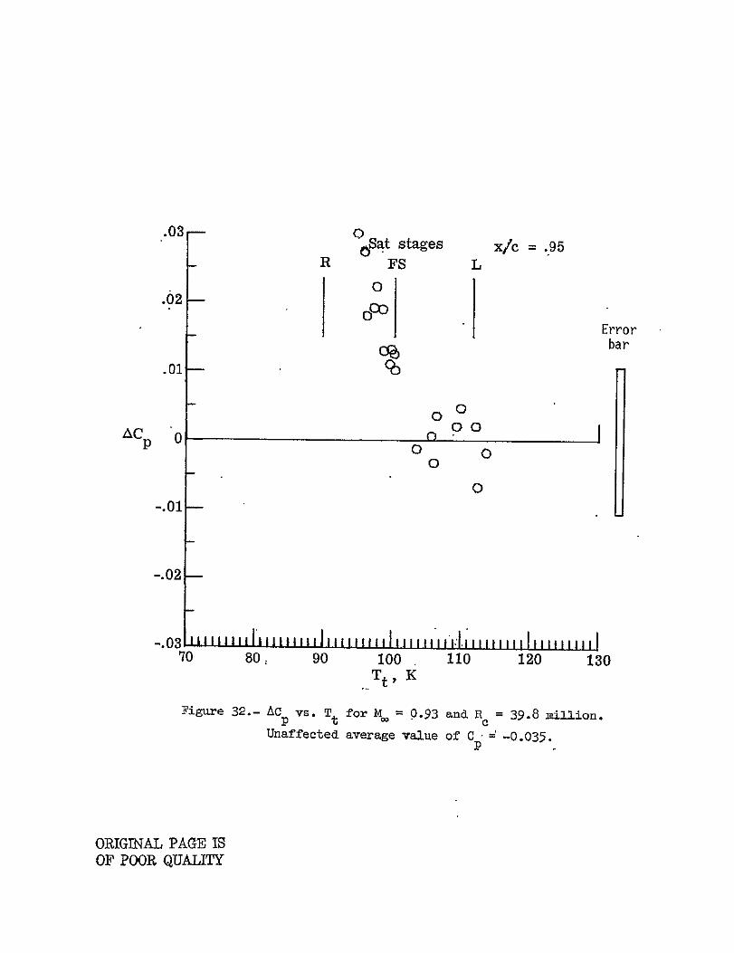
distribution of onset Tt. The lack of'resolution is indeed unfortunate as

seen in figure 32, which shows AC vs. Tt for x/c = 0.95, because there

are no effects at Tt = 103.5 K but well developed effects at 100.5 K. For

this path, onset Tt for the airfoil was chosen to be 102.0 K with the error

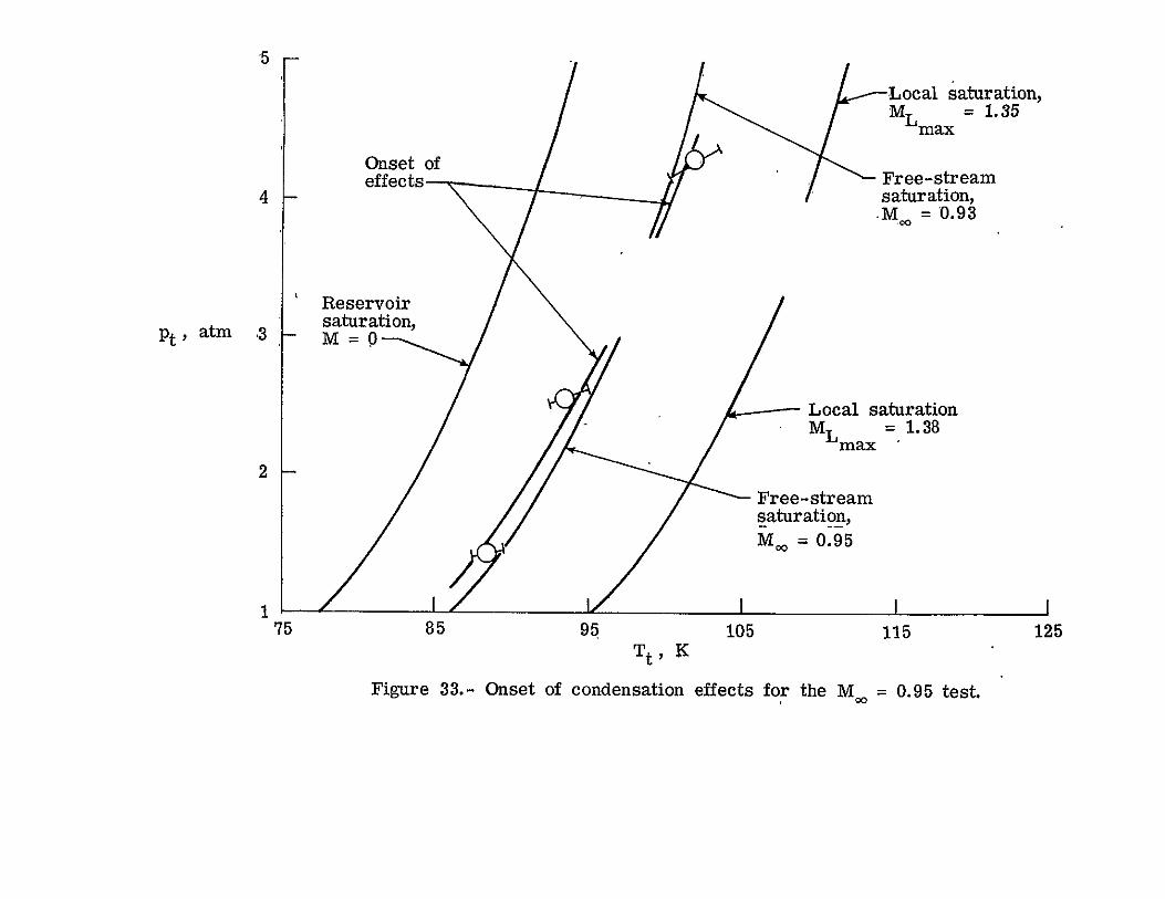
bar spanning 100.5 to 103.5 K. The summary plot for onset conditions for the

M = 0.95 test is given in figure 33.

The results for all of the M tests will now be gtouped together assuming

first that ML is the important Mach number parameter and then assuming max

that M. is the important parameter. The question of which Mach number is

important arises because of the uncertainty in the mode of nucleation that is

occurring, which is discussed in the next section.

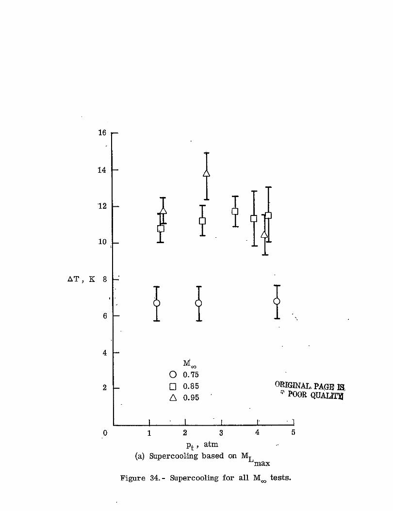
The first pair of figures comparing all of the onset results is constructed

for the supercooling as defined in equation (1).

AT = T -T (1) s e

In equation (1), the value of T is the static temperature at which the s

isentrope, starting at the onset values of Pt and Tt, crosses the vapor­

pressure curve. The value of Te is the static temperature along the same

isentrope at M = MI in figure 34 (a) and at M = M in figure 34(b). max

PAGEo9

15OFP00i3 -Q1ALY

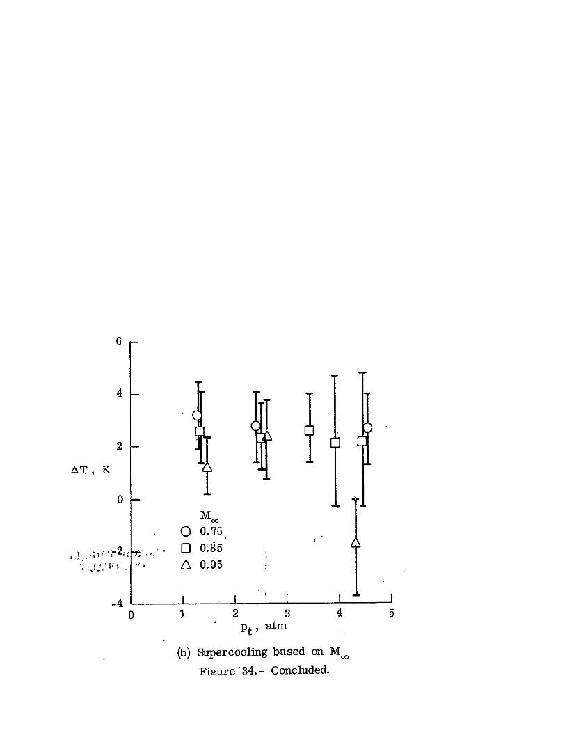
In both cases the value of AT is plotted as a function of the onset Pt along

each path of constant R . In figure 34(a), the supercooling was nearly constant

at 7 K over the pressure range for Mb = 0.75, was roughly equal to 11 K over

the pressure range for M = 0.85, and was 12 and 14 K for the two lower

pressure paths at M. = 0.95 and then dropped to 10 K for the high pressure path.

In figure 34(b), the supercooling based on M remained between 2 and 3 K over

the pressure range for both M. = 0.75 and' 0.85. However, the supercooling for

the b = 0.95 test was 1 and 2 K for the lower pressure paths, but dropped to

-2 K for the upper pressure path. Regardless of the behavior of the high pressure

path for the M = 0.95 test, there seems to be-much better correlation of the

values for supercooling when assuming N is the pertinent Mach number rather

than ML max

The second pair of figures again compares all of the onset results, but the

comparison is now made in a logl 0 p versus T plane. Static values of p, T

are calculated from the Pt and at onset and are calculated assuming anTt

isentropic expansion to either ML or M.. Figure 35(a) shows the p, T max

as calculated assuming ML is the'Mach number of interest while figure 35(b) max

shows the p, T as calculated assuming M. is the important Mach number. it

would again appear from figure 35, as in figure 34, that the onset data correlates

much better with K than with ML max

The seemingly early onset of effects in the high pressure path of the

= 0.95 test may be the result of a tunnel configuration change that was made

before the data for this path was taken. The spray bars system used for injection

of the liquid nitrogen as described under the tunnel apparatus was removed for

another investigation in the .3-m tunnel and remained out for the tunnel entry

during which the data was obtained for the high pressure path of the MW = 0.95

test. With the spray bars removed the liquid was injected from four nozzles

16

flush with the interior tunnel wall at injection station 1 instead of the

eleven nozzles at the three different stations. Consequently, the liquid

injected may not have broken up and evaporated as effectively as it did with

the eleven nozzles. The unevaporated drops may have formed the increased number

of nucleating sites necessary to decrease the amount of supercooling realized.

Because of this uncertainty due to the tunnel configuration change, the data

from the high pressure path of the M = 0.95 test will-not be presented in

further data comparison graphs.

Implications of the Data

Condensation effects can be caused by three different modes of nucleation,

where nucleation is taken as the formation of a stable liquid droplet. The

three different modes are homogeneous, heterogeneous, and binary nucleation.

These three processes differ by the manner in which they overcome an energy

barrier to droplet formation and hence growth. In depth discussion of the

three types can be found in references 2, 3, 4, 10, 11, 12, and 13. The

different modes can briefly be summarized as follows.

Homogeneous nucleation can occur when the gas undergoes supercooling, which

will decrease the energy barrier to liquid droplet formation. When enough

supercooling occurs, the gas molecules will be able to overcome the energy

barrier to droplet formation and massive nucleation rates are likely. Hetero­

geneous nucleation may occur when there are liquid or solid impurities

suspended in the vapor at the time the flow first expands past the vapor­

pressure curve and begins to supercool. The energy barrier of formation,

which is so important for homogeneous condensation, is not so significant here

because the impurities can act as a catalyst for the condensation process.

QO 17

Consequently, little or no supercooling is needed before stable droplet growth

occurs. What prevents heterogeneous nucleation from always dominating the

homogeneous process is that it requires extremely large concentrations of

impurity sites to influence the flow as was pointed out by Wegener and Mack

in reference 2. The third type of nucleation possible is binary. This process

occurs when a mixture of two different gases condenses into droplets which are

composed of both types of molecules. The binary process is discussed

specifically in references 10 to 13. The combination of the two species can

effectively change the energy barrier to nucleation in such a manner that

condensation will occur earlier than analysis would predict for either of the

species acting singly.

The data from the present experiment does seem to suggest which nucleation

process might have occurred. First, no condensation seems to be occurring until

at least 7 K of supercooling has taken place at the M. location. If binary max

nucleation is occurring with some sort of impurity vapor in the nitrogen used

for cooling the tunnel, then its effects were either undetectable or occurred

at low enough temperature to be confused with homogeneous or heterogeneous

nucleation of the nitrogen test gas. The purity of the liquid nitrogen injected

for cooling was approximately 99.95 percent in the present experiments, so it is

assumed that binary nucleation would be unlikely. Second, none of the orifice

onset Tt versus x/c plots show any systematic trend toward condensation first

appearing in the region of maximum supercooling, which is the region of high

local Mach number. Since the amount of supercooling is so important for

homogeneous nucleation, these results do not seem consistent with what one would

expect if homogeneous nucleation was occurring. In fact, there seems to be no

18

generally preferred location over the airfoil for effects to occur. Hence the

effects may actually be the result of heterogeneous nucleation occurring upstream

of the model in the test section. Under these circumstances the airfoil would

experience the influence of these droplets over its length at about the same Tt

although local sensitivity to the condensate in the free-stream may vary over the

airfoil because of differences in ML or pressure gradient. If condensate in

the free-stream is the cause of the effects, the possible source for the impurity

sites could be the injected liquid nitrogen used for cooling the tunnel. At the

very low temperatures of these tests, the injected liquid may not be completely

evaporating in the time it takes to travel from the injection stations to the

test section (see figure 2). The partially evaporated droplets may provide the

high concentration of nucleation sites needed for heterogeneous condensation.

Some evidence for heterogeneous nucleation from unevaporated drdnlets in the

free-stream comes from figures 34 and 35, which show stronger correlation

between the onset of effects and M than the onset of effects and ML

maxFurther evidence comes from the smaller amount of supercooling realized with

the high pressure path of the M = 0.95 path. Because the configuration without

spray bars is less efficient at breaking up the injected liquid nitrogen, it

would seem that the smaller amount of supercooling was due to an increased

number of liquid drops on which condensation growth could occur. Light

scattering tests should be made in the test-section to determine conclusively

if indeed there are unevaporated .injection droplets.

Comparison to Other Works

While it appears that heterogeneous nucleation is the cause of condensation

in the present experiments, most of the previous condensation investigations have

19

concentrated on homogeneous nucleation. Some of these investigations were

cqoncerned with nitrogen gas, and two references, 14 and 15, will be used here

for comparison to the present data. A traditional means of presenting onset of

effects data is in the lOglo p vs. T plane. As mentioned in the previous

section, there is some question as to the process of nucleation and hence in

the relevant condition to plot in the log1 0 p vs. T plane. For the present

comparisons, it was decided to use the static values of p and T as calculated

for the ML condition because regardless of the source of the effects, this max

amQunt of supercooling was realized in the region of maximum local Mach number

before effects were detected.

Using the log10 p vs. T format, the present results can be compared with

the analytical nitrogen-gas work done by Sivier in reference l. His computer

cqmputations assumed homogeneous nucleation and used classical liquid droplet

theory. An unpublished curve fit by Adcock to Sivier's calculated onset points

for conditions of higher pressure and lower onset Mach number has been plotted

along with the present onset conditions in figure 36, where Adcock's curve- fit

is represented by

10-2 1 1.461 x 4.,962 x 10 3 1 0 p + 2- x lOg 1.959 x (2)

T e 910 P+ 1959x 1 xClog10 p

There is good agreement in trends between the curve fit to Sivier's prediction

and the present results although the present onset points fall closer to the

vapor-pressure curve than predicted. If Sivier Is calculations are accurate. the

results would imply that effects are occurring earlier than predicted for

homogeneous nucleation. Again, heterogeneous nucleation would be consistent

20 ORIGINAL PAGE ISOF POOR QUALITZ

with the data. However, many of the M = 0.85 and 0.95 onset points do

approach Sivier's onset line for homogeneous nucleation. If heterogeneous

nucleation is indeed occurring then significantly more supercooling may not be

possible for the M. = 0.85 and 0.95 tests even if the impurity sites were

eliminated and homogeneous nucleation took place.

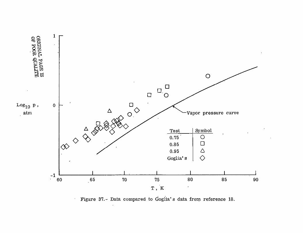
The present results can also be compared to previous experimental results.

Goglia in reference 15 has taken data that shows nitrogen onset in the same

static pressure and temperature range as considered in the present study.

When Goglia's data and the present experimental data are plotted together,

as in figure 37, the agreement is especially good considering the fact that the

present data consisted of subsonic and supersonic onset points over a 0.137-m

airfoil and Goglia's work consisted of rapid expansions in a 0.31 4-m long nozzle a

onset at Mach numbers from 2.0 to 3.25. Although one would normally expect

more supercooling with the larger velocity gradients in the nozzle, it does

not show up in the data comparison. In fact, the trend of Gcglia's data falls

close to the present M. = 0.75 data but seems to have somewhat less super­

cooling than was experienced during the present M = 0.85 or 0.95 data. Goglia

states in his conclusion that the condensation he detected

appeared to be the result of the self-nucleation, or homogeneous condensation,

of the nitrogen test gas. However, the gas used by Goglia was only 95 percent

pure nitrogen and contained a 5 percent impurity of oxygen. Even though this

fact was well recognized and investigated by Goglia, there may be some effects

of heterogeneous nucleation on his onset points. (Arthur and Nagamatsu in

reference 6 detected a mild decrease in supercooling of about 1 to 2 K for a

5 percent oxygen impurity.)

21

Whether or not the condensation in the present investigation was the result

of heterogeneous or homogeneous nucleation, it appears that the magnitude of the

supercooling is comparable to what others have seen or predicted in the same

pressure range.

Benefits Realized

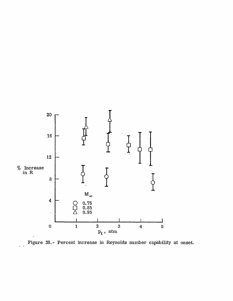
One of the primary motivations for the present experiments was to determine

the increase in Reynolds number capability that might be possible when testing

an airfoil with supercooled flow. This increase was determined for the NACA

0012-64 airfoil and figure 38 shows the percent increase realized at the tem­

perature at which condensation effects were first detected. The percent increase

was calculated by (1) dividing Rc corresponding to Pt and Tt at onset

by Rc corresponding to Pt at onset but with Tt being that which just allows

local saturation, (2) subtracting one from the resulting ratio, and (3) multiplying

by one hundred. As can be seen in figure 38, the M = 0.75 test realized the

smallest percent gain in capability at 7%, while the M = 0.95 test realized

the largest at 19%. The M = 0.75 and 0.85 tests appear to show a decrease in

gain with increasing Pt, while a trend for the M = 0.95 test cannot

easily be predicted because of -the lack of a high pressure path data point.

Error bars shown are calculated from the uncertainty in the value of Tt for the

onset of condensation effects over the airfoil.

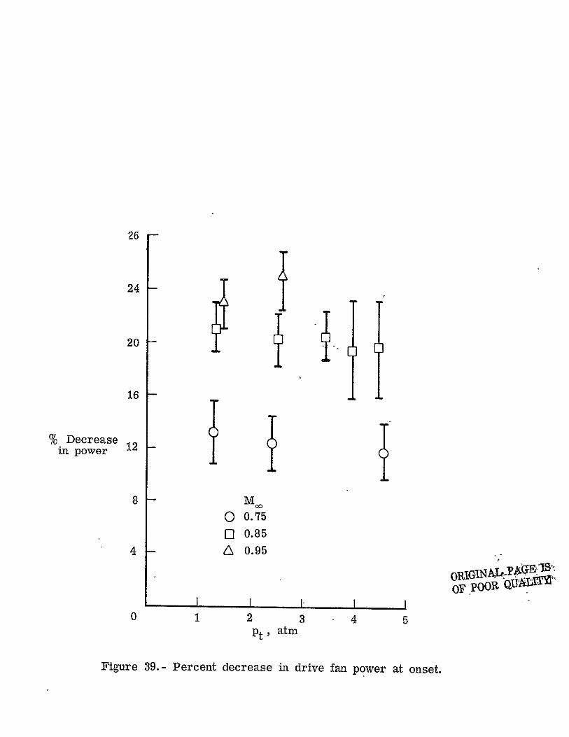
The second motivation for the present experiment was to determine percent

decreases in drive fan power required and in the amount of liquid nitrogen (LN2)

injected when unit Reynolds number is held constant and the supercooling is

utilized to decrease both Pt and Tt. Since the energy required for producing

22

the amount of LN2 injected is much greater than the energy used by the drive fan,

reductions in direct operating costs while at test conditions will be much

closer to the percent decrease in LN2 required than to the decrease in drive

fan power required.

The decrease in drive fan power realized is shown in figure 39. The

trends are, of course, similar to the increase in Reynolds number capability

shown in figure 38. For M = 0:85 the decrease in drive power required varied

from 21% at low pressure to about 19% at the high pressure end. Decreases of

23 and 25% were found for the two low pressure paths in the = 0.95 test.

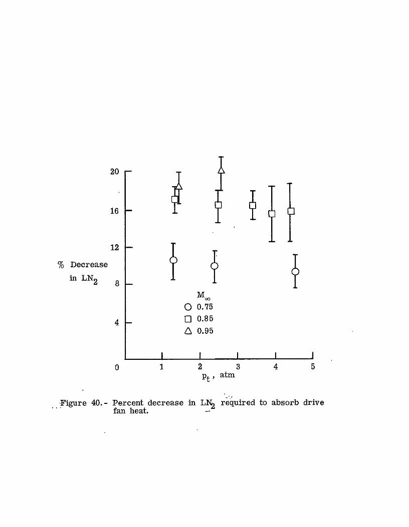
The decrease in LN2 required to absorb drive fan heat is shown in figure 40.

For an insulated tunnel such as the Langley 0.3-m tunnel, the injected LN2

required to absorb the heat flow into the tunnel through the tunnel shell

insulation is relatively constant ov&r the temperature range of the present tests

and is only on the order of I percent or less of the amount required to absorb

the heat of the drive fan. Consequently, heat leakage through the shell, has

no effect on figure 40 and has not-been included. For the Mk - 0.T5 test, the

reductton in LN2 required varied from 1% down to 9% at "the higher pressures.

For'Mb = 0.85, the reduction varied from 17% at the lower pressures to 15%

at the higher pressures. The M = 0.95 test had a reduction high of 20%

and a low Of 18%.

23

CONCLUDING REMARKS

An experimental program was undertaken to determine the onset of conden­

sation effects in the pressure distribution about a 0.137-m NACA 0012-64

airfoil tested in the Langley 0.3-m transonic cryogenic tunnel at free-stream

Mach numbers of 0.75, 0.85, and 0.95 over a total pressure range from 1;2 to 5;0

atmospheres. -Orifice pressure measurements were recorded at 5% chord intervals

and were analyzed to determine the total temperature at which deviations first

occurred in the orifice pressure coefficient.

The onset of condensation effects were found to correlate more with the

amount of supercooling in the free-stream than with the supercooling in the

region of maximum local Mach number over the airfoil. Effects in the pressure

distribution over the airfoil were generally seen to appear over its entire

length at nearly the same total temperature. Both observations suggest the

possibility of heterogeneous nucleation occurring in the free-stream.

Comparisons of the present onset results are made to calculations by Sivier

and data by Goglia.

The potential operational benefits of the supercooling realized were

analyzed in terms of increased Reynolds number capability at a given tunnel

total pressure, reduced drive fan power if Reynolds number is held constant,

and reduced liquid nitrogen consumption if Reynolds number is again constant.

Depending on total pressure and free-stream Mach number, these three benefits

are found to respectively vary from 7 to 19%, 11 to 25%, and 9 to 20%. Since

operating costs at typical test conditions are approximately 10% due to fan

drive-power and 90% due to liquid nitrogen injection, reduction in operating

24,

costs will be very close to the percentage reduction in liquid nitrogen con­

sumption.

Although the present experimental data form a preliminary basis for

predicting minimum operating temperatures for nitrogen-gas wind tunnels, it is

just one of several steps that are needed for a more complete understanding of

the problem. More work is needed in the following areas: tests of other airfoil

pressure distributions to determine the sensitivity of the onset of condensation

effects to different local velocities and gradients, experiments designed to

determine conclusively if condensation is caused by homogeneous or heterogeneous

nucleation, studies to determine scaling effects so that the present results may

be extended to other sizes of tunnels, and studies to extend the results to

higher total pressures.

25

APPENDIX A

DATA ANALYSIS PROCEDURE

Because of the importance of the data reduction technique upon the detection

of the onset of condensation effectsi this appendix is included in order to

describe in detail the M1 correction procedure and to explain the procedure

for determining airfoil onset Tt . Examples of the various steps are included

for the b= 0.85 and Rc = 16 million path.

The Mb correction procedure was employed in order to take out as much

Mach number effects as possible when comparing C 's along a path of constant p

M and Ra. While M0 was nominally constant along a path, many pressure

distributions were recorded at values of 'M1 that varied from the nominal value

by ±.010o To determine if a M0, dependence did exist at a given x/d location;

a linear regression technique was applied to condensation-free values of CP

plotted as a function of M.. In this manner, if there was a correlation

between Cp and M , all of the data could be corrected to a single value of

M . If there was little correlation between C and M , then a weak dependence

was assumed to exist and no correction was assumed necessary. Thus all the

data along a given path of constant M ~cand R could be utilized,

The first step of the M correction procedure is to apply a linear

regression technique to values-of C at a given x/c as a function of M..P .

Using standard definitions as found for example in reference 16, the slope

of the linear regression fit would be given by

26

n S(Mi - )(C - p)

m=1 ip (Al)

i=l i

where

n Z M.

R- i=l ± (2)Co n

and

n Z C

i=l Pi (3)

p n

The correlation coefficient, r, which is an indication of goodness of fit is

given by

n S (M W - )(c - )

r- 1 (A4) - ,)2(M (C

1S n (0 2 i1 i l P

where if r = 0 there is no correlation and if Irl = 1 then there is perfect

correlation. For the present analysis if Irl > 0.5, then the correlation is

considered strong enough to use m in correcting a given M. to another

value. If Irl < 0.5, the dependence between C and M is considered weak,p

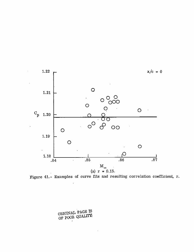
and m is assumed to be zero. Three examples of various values of r are

shown in figure hi for the M = 0.85 and Re = 16 million path. Figure 4i(a)

shows the value of Cp for x/c = 0.00 (the orifice at the leading edge of

the airfoil) as a function of M. In this case r = 0.15 and, indeed, there

seems to be little correlation between M and C . Consequently, no attempt p

PAGE 19OtRIGNAL ()Og QUALITYOF 27

is made to manipulate or correct this data for small differences in M.

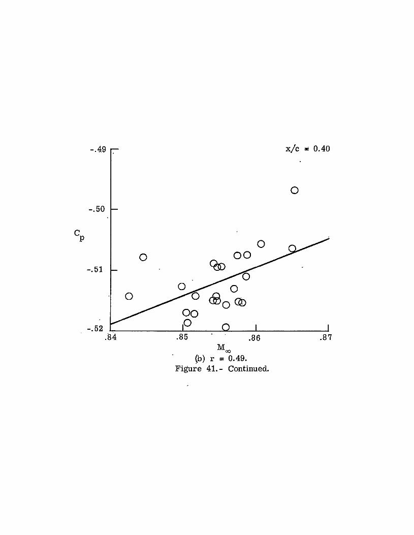
Figure 41(b) shows the values of C for x/c = 0.40 as a function of MM.

In this case r = 0.49, and so this linear curve fit barely fails to meet the

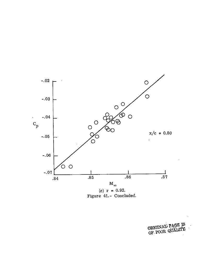
correiation test. Figure 41(c) illustrates the values of CP for x/c = 0.80

that lead to a value of r equal to 0.92. As seen in figure 41(c), there is

good correlation between C and M., and differences in C due to'differences

in M can be removed by correcting values of C to a given M by setting p 0

C = C - m • (M - MW ) (A5)

where C is the corrected value of C and m is the slope of the linearP0 P

fit. Again, m is assumed to be equal to zero if Irl < 0.5.

Once the linear regression technique has been applied to the values of CP

for each orifice along the path, a set of intermediate graphs are drawn before

the airfoil onset Tt is determined. For each orifice a value of AC is

plotted as a function of Tt where

AC = C - C P PO Pave (A6)

In equation (A6), C is corrected with respect to M and C is an Po Pave

average of condensation-free values of C for that orifice. (Condensation­

free values were determined by establishing crude onset values of withoutTt

the benefit of correction procedures and then adding at least a 2 K temperature

buffer. Final onset values of T were then checked to insure that C t Pave

was indeed free from condensation effects.) An example of a AC vs. Tt

28

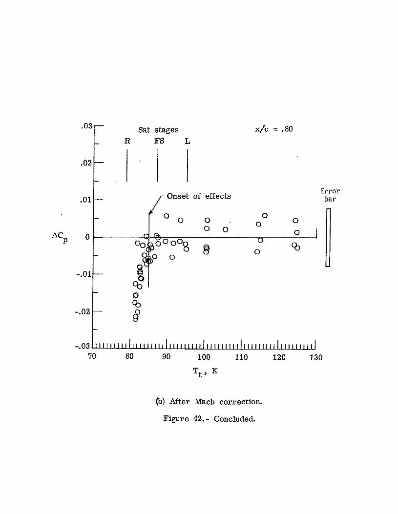
with and without correction is shown in figure 42 for x/c = 0.80 and where

r = 0.92. Figure 42(a:) shows the uncorrected data while figure 42(b) shows the

values of C after being corrected. As can be seen, considerable "order" is p

added to the data by the correction process and this "order" permits easier

identification of the Tt at which Cp at this x/c locatdoff begins to

depart from its unaffected average value. Not always, however, was Irl > -5

and so this simplification was not always possible. Graphs similar to fig­

ures 42(a) or 42(b) are then drawn for each orifice location over the airfoil.

These graphs are used to determine at what each of the orifices firstTt

experience systematic departure from its unaffected average value of CPO

These orifice onset temperatures are then plotted as a function of x/c

as was shown in figure 20. These orifice onset T vs. x/c plots are the t

key analysis graphs because they provide an overview of the effects on the

airfoil as a whole. There is experimental uncertainty in the onset point for

each orifice and consequently it is helpful to see all of the orifice onset

Tt's together so that a particularly low or high value can be checked for

possible error. The airfoil onset Tt is not taken to be an average of

orifice onset. Tt's , but rather is taken to be the warmest orifice onset Tt

that appears systematic. Uncertainty bars are normally drawn to encompass

the highest orifice onset Tt, whether the deviation appears systematic or not.

The data analysis procedure described herein was more sensitive'to

condensation onset than previous analyses described in references 17, 18 and

19. In references 17 and 18 pressure distributions were superimposed to detect

differences - no correction was made to Cp for differences in M and,

consequently, much of the data could not be used. Reference 19 utilized the

AC vs. T format at 0, 25, 50, and 75 percent chord locations but still did p t

not include the Mach correction technique.

29

APPENDIX B

ERROR ANALYSIS FOR ACp VS. Tt -GRAPHS

During the present experiment, fluctuations in wind tunnel conditions were

the prime source of error during the 50 second period required to record the data.

Tunnel conditions were observed to fluctuate with standard

deviations of the following approximate magnitudes: aPt of +.005 atm (varied with Mand

R ); am of ±.003; and oTt of ±0.5 K. The manufacturer's stated uncertainty in

the static pressure measurements' Ap, was 0.5% of full scale. A representative

standard deviation for AC due to these fluctuations is calculated herein p

using normal error propagation techniques, see reference 20 for example.

As defined in equation (A6),

ACp = C - C (A6)P o Pave

in which C is the value of the pressure coefficient, corrected to-some P0

value of free-stream Mach number, M, from data taken at a free-stream 0

Mach number of M. The correction is defined as

C = C -m ( - M) (A5)

where m is the slope of the linear regression fit as defined in equation (Al).

If sufficient correlation, r, as defined in equation (A),is not found, m

is assumed to be equal zero. Since CPave is just the average of the corrected

condensation-free data, the variance of C can be approximated byPave

30

C

2 C

2 PO (Bi) Pave

where N would be the number of samples used in the average. The variance of

can be written from equation (A5) as * Po

2 2 2 aC =aC +aF (B2)

PO P

where F is defined as

F = m(M. - MW )(B3) -0

Assuming there is much more relative error in (M - M ) than m, the variance 0

in F will be primarily due to the variance in the difference in Mach numbers.

Since M. is an arbitrarily defined constant, we may write' 0

2 22 (B4)aF ma,,.

Consequently, equations (A5), (A), (Bi), (B2), and (B3) lead to

2A N -lU2 + m~ca (B5)

It now remains to discuss , the variance associated with error in the 'p

values of C before Mach correction. The value of C is defined as p p

p - p0C = (B6)

ORIGflN' PAGE IS OF pOOR QUALITY

31"

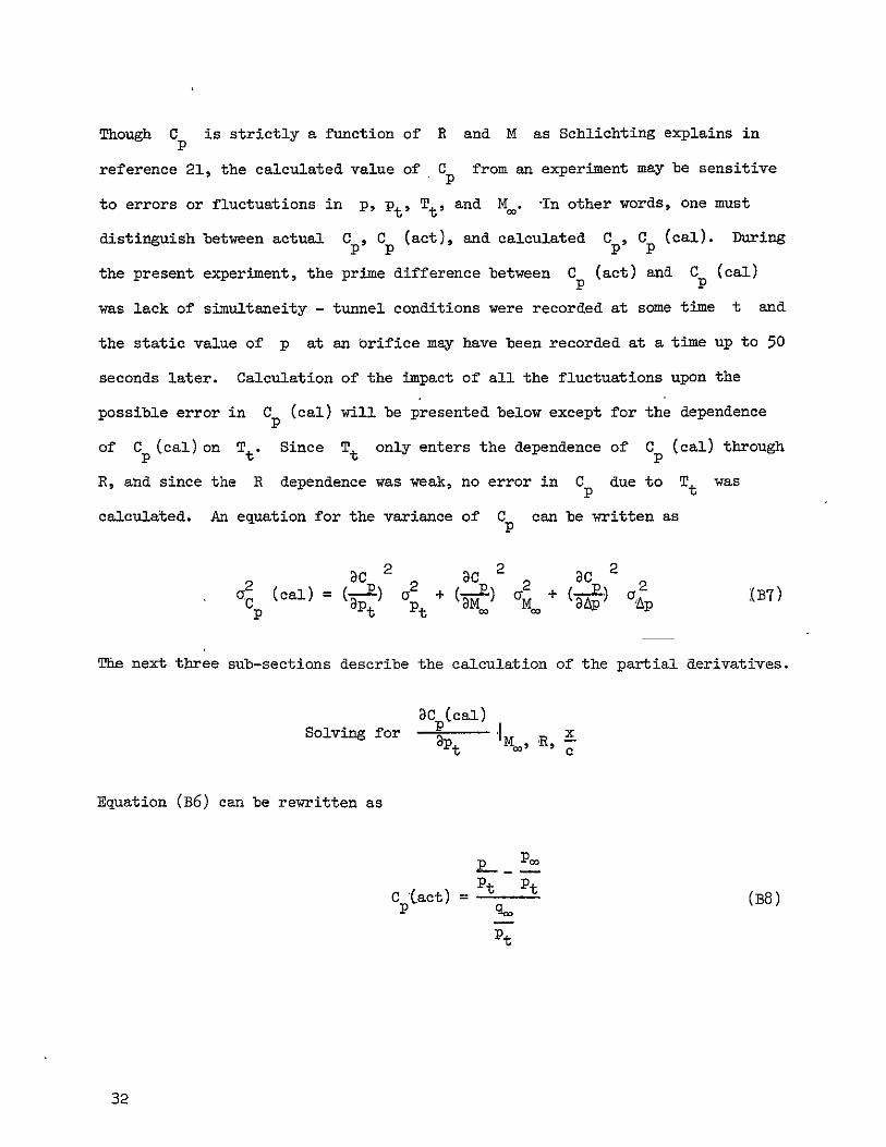
Though C is strictly a function of R and M as Schlichting explains inP

reference 21, the calculated value of C from an experiment may be sensitive

to errors or fluctuations in p, pt, Tt, and M.. -In other words, one must

distinguish between actual Cp, Cp (act), and calculated Cp, Cp (cal). During

the present experiment, the prime difference between C (act) and C (cal)P P

was lack of simultaneity - tunnel conditions were recorded at some time t and

the static value of p at an orifice may have been recorded at a time up to 50

seconds later. Calculation of the impact of all the fluctuations upon the

possible error in C (cal) will be presented below except for the dependenceP

of Cp (cal) on T . Since Tt only enters the dependence of Cp (cal) through

R, and since the R dependence was weak, no error in Cp due to Tt was

calculated. An equation for the variance of C can be written as

C2 2 C2

2 (cal) 20 + 2 a 2

The next three sub-sections describe the calculation of the partial derivatives.

SCp(cal) Solving for pt, R, x

Equation (B6) can be rewritten as

pp0tc)= q (B8)

Pt

32

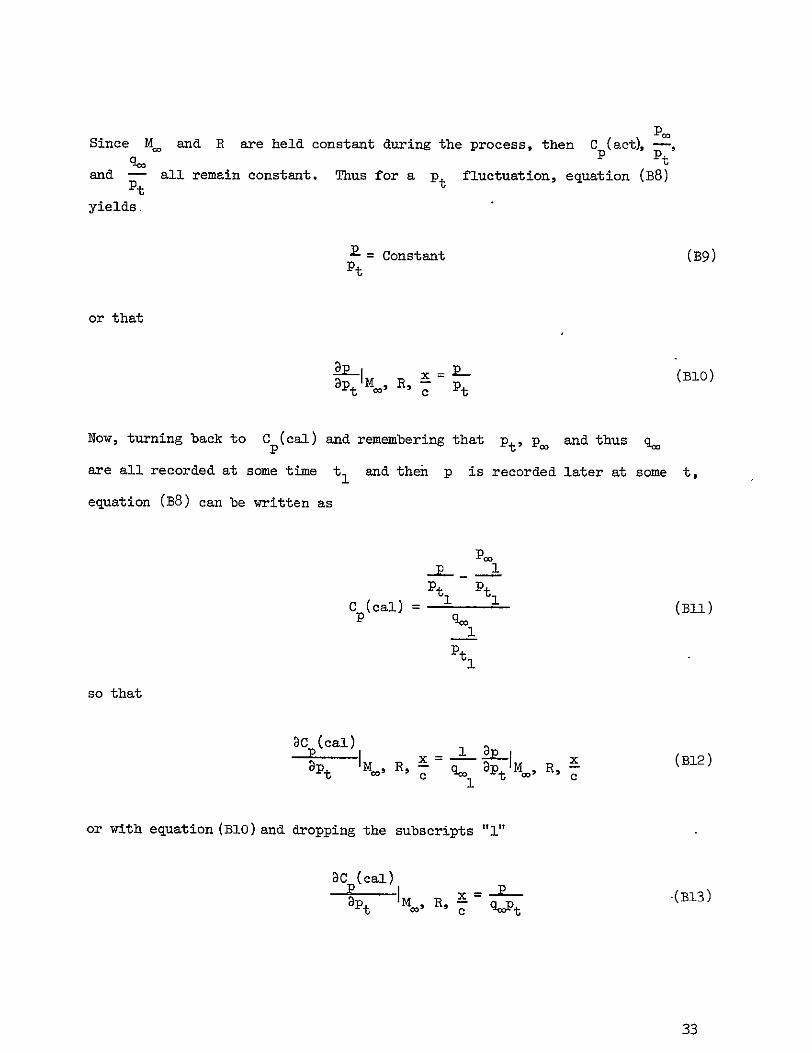
Since 14 and R are held constant during the process, then C (act), -,

q. p Pt

and - all remain constant. Thus for a Pt fluctuation, equation (B8) Pt

yields

P Constant (B9)Pt

or that

3p 114 R (Blo) t ,, c Pt

Now, turning back to Cp(cal) and remembering that pt, p. and thus ql

are all recorded at some time t and theh p is recorded later at some t,

equation (B8) can be written as

P. p - 1

Cp (cal) Pt= Pt (Bll)

pp Pt1

so that

DC (cal) (Bl2) c 1 Pt , c

or with equation (Blo) and dropping the subscripts 'T'

DC (cal)

-(BI3)I x = ,c qPt

33

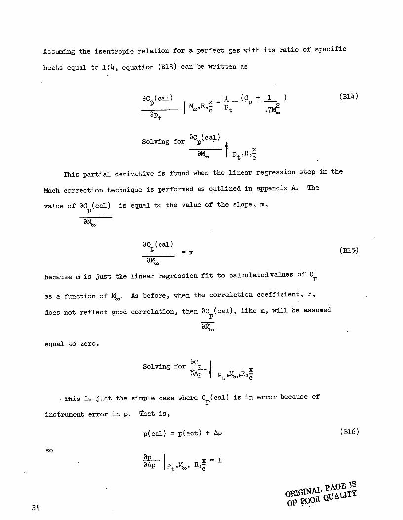
Assuming the isentropic relation for a perfect gas with its ratio of specific

heats equal to 1.14, equation (B13) can be written as

DC-(cal) 1 (C + 1 ) (B14)

apt

Solving for ap(cal)

This partial derivative is found when the linear regression step in the

Mach correction technique is performed as outlined in appendix A. The

value of 30 (cal) is equal to the value of the slope, m,

30 (cal) = (B15) (Bl5

because m is just the linear regression fit to calculated values of C

p

As before, when the correlation coefficient, r,as a function of M .

does not reflect good correlation, then Cp (cal), like m, will be assumed

equal to zero.

Solving for a x

3Ap I pttoRDM c

This is just the simple case where Cp(cal) is in error because of

instrument error in p. That is,

(B16)p(cal) = p(act) + Ap

so

op IGINA'A G IS or pooQ­34

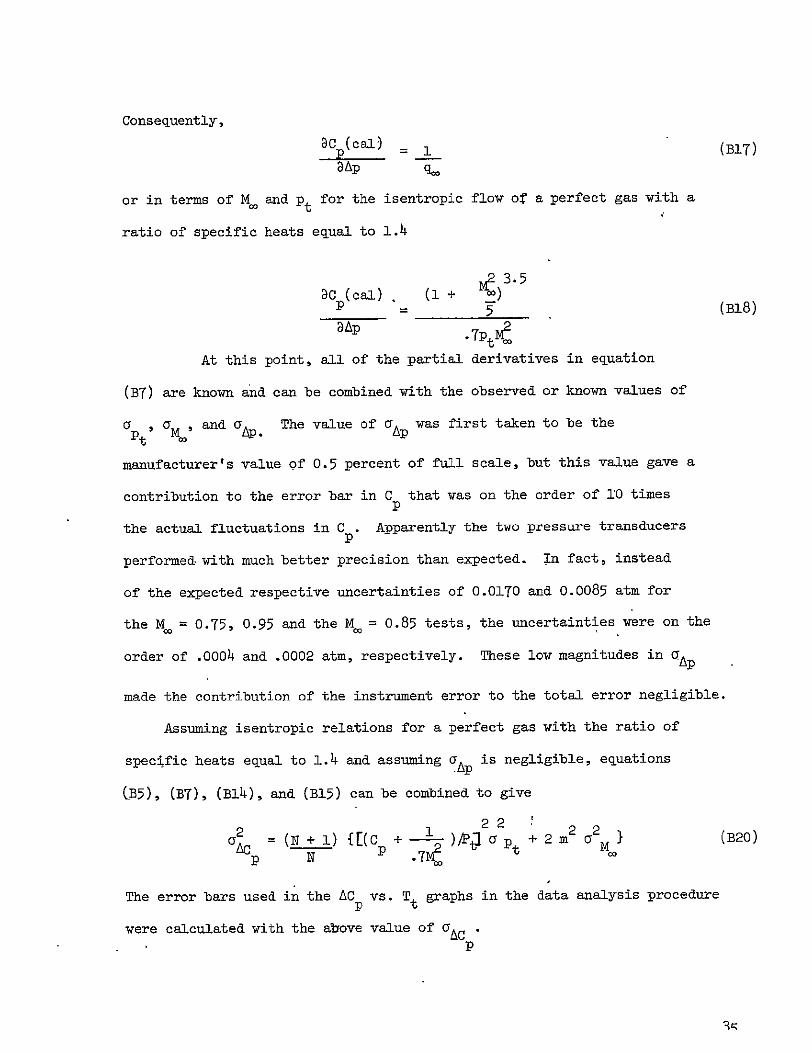
Consequently,

30 (cal) B7 3Ap q.

or in terms of M and Pt for the isentropic flow of a perfect gas with a

ratio of specific heats equal to 1.4

Bi)3

(i +3C (cal)

_ (B18)

3Ap . MPt2

At this point, all of the partial derivatives in equation

(B7) are known and can be combined with the observed or known values of

rPt , ,aand aAp . The value of a p was first taken to be the

manufacturer's value of 0.5 percent of full scale, but this value gave a

contribution to the error bar in C that was on the order of 10 times p

the actual fluctuations in C . Apparently the two pressure transducersP

performed with much better precision than expected. In fact, instead

of the expected respective uncertainties of 0.0170 and 0.0085 atm for

the M = 0.75, 0.95 and the M = 0.85 tests, the uncertainties were on the

order of .0004 and .0002 atm, respectively. These low magnitudes in Ap

made the contribution of the instrument error to the total error negligible.

Assuming isentropic relations for a perfect gas with the ratio of

specific heats equal to 1.4 and assuming a is negligible, equations.AP

CB5), (B7), (BI4), and (B15) can be combined to give

2 1 2 2 2 = (N + i) {t(c +- P 2 a 4 (B20)

pC N p 7e .t tM

The error bars used in the ACp vs. Tt graphs in the data analysis procedure

were calculated with the above value of AC P

REFERENCES

1. Adcock, Jerry B.: Real-Gas Effects Associated with One-Dimensional Transonic Flow of Cryogenic Nitrogen. NASA TN D-8274, 1976.

2. Wegener, P. P.; and Mack, L. M.: Condensation in Supersonic and Hypersonic Wind Tunnels. Advances in Applied Mechanics, Vol. V, 1958, pp..307-47.

3. Wegener, Peter P.: Nonequilibrium Flow with Condensation. Acta-Mechanica 21, 1975, pp. 65-91.

4. Daum, Fred L.; and Gyarmathy, George: Condensation of Air and Nitrogen in Hypersonic Wind Tunnels. AIAA Journal, Vol. 6, No. 3, Mar. 1968, pp. 458-465.

5. Goglia, Gennaro L.; and Van Wylen, Gordon J.: Experimental Determination of Limit of Supersaturation of Nitrogen Vapor Expanding in a Nozzle. Journal of Heat Transfer, Vol. 83, Series C, No. 1,- Feb. 1961, pp. 27-32.

6. Arthur, P. D.; and Nagamatsu, H. T.: Effects of Impurities on the Super­saturation of Nitrogen in a Hypersonic Nozzle. Hypersonic Wind Tunnel Mem. No. 7, Guggenheim Aeronaut. Lab., Calif. Inst. of Technol., Pasadena, California, 1952.

7. Adcock, Jerry B.; and Ogburn, Marilyn E.: Power Calculations for Isentropic Compressions of Cryogenic Nitrogen. NASA TN D-8389, 1977.

8. Kilgore, Robert A: The Cryogenic Wind Tunnel for High Reynolds Number Testing. Ph. D. Thesis, University of Southampton, 1974.

9. Kilgore, Robert A.: Design Features and Operational Characteristics of the Langley Pilot Transonic Cryogenic Tunnel. NASA TM X-72012, 1974.

10. Stauffer, D.: Kinetic Theory of Two-Component ("Heteromolecular") Nucleation and Condensation. J. Aerosol Sci., Vol. 7, 1976, pp. 319-333.

1l. Wegener, Peter P.; and Wu, Benjamin, J. C.: Homogeneous and Binary Nucleation: New Experimental Results and Comparisons with Theory. Faraday Discussions of the Chemical Society, No. 61 Precipitation, 1976.

12. Wilemski, Gerald: Binary Nucleation. I. Theory Applied to Water-Ethanol Vapors. Journal of Chemical Physics. Vol. 62, No. 9, May 1975, pp. 3763-3771.

13. Wilemski, Gerald: Binary Nucleation. II. Time Lags. Journal of Chemical Physics, Vol. 62, No. 9, May 1975, pp. 3772-3776.

36

14. Sivier, Kenneth D.: Digital Computer Studies of Condensation in Expanding One-Component Flows. Aerospace Research Laboratories Report ARL 65-234, November 1965.

15. Goglia, Gennaro L.: Limit of Supersaturation of Nitrogen Vapor Expanding . in a Nozzle. Ph. D. Thesis, University of Michigan, 1959.

16. Freund, John E.: Mathematical Statistics. Second ed. Prentice-Hall, Inc., 1971.

17. Hall, Robert M.: Preliminary Study of the Minimum Temperatures for Valid Testing in a Cryogenic Wind Tunnel. NASA TM X-72700, 1975.

18. Hall, Robert M.; and Ray, Edward J.: Investigation of Minimum Operating Temperatures for Cryogenic Wind Tunnels. Journal of Aircraft, Vol. 14, No. 6, June 1977, pp. 560-564.

19. Hall, Robert M.: An Analysis of Data Related to the Minimum Temperatures for Valid Testing in Cryogenic Wind Tunnels Using Nitrogen as the Test Gas. NASA TM X-73924, 1976.

20. Crandall, Keith C.; and Seabloom, Robert W.: Engineering Fundamentals in

Measurements, Probability, Statistics, and Dimensions. McGraw-Hill, 1970.

21. Schlichting, Hermann: Boundary-Layer Theory. Sixth ed. McGraw-Hill, 1968.

Gas properties Test conditions and 4p 8 drive power

Reynolds number, R 3 -6 -

Values relative 2 4­to 322K

12 - Dynamic pressure, q 7

t1Power I I I I

0 100 200 300 400 0 100 200 300 400

Stagnation temp, K

(a) (b)

Figure 1.- Effect of temperature reductioi for M. = 1.0, constant Pt

and 'constant reference length.

-LN2 Stations no. 2 and 3

Nacelle section

Tunnel anchor

Figure 2.- Schematic of Langley 0.3-m transonic cryogenic tunnel.

1 2 3 4 5 6 7 8 9 10 11 12 13 14 15 16

x c - 0.137 m

Figure 3.- Two dimensional NACA 0012-64 airfoil has orifices spaced at 5 % chord locations. trailing edge orifice was added for tests with M. = 0.75 and 0.95.

5

Free-stream­saturation,

M = 0.85 Local satfiration over airfoil,

4 ML = 1.2 4 max

Reservoir saturation, M=0

pt arm 3

2

75 85 95 105 115 125 Tt K

Figure 4.- Region of interest for the M 0.85 test.

5- 38&X 06 42'× 106'/

saturation;. MoO.=0.85

p26

Reservoir. saturation,,x/0

2

x 106'

,-----Rec = 16, x.106

75 85' 9&0.5 115,, 125

Tt K Figure 5.-- Path of constant R. for the =. 0.&5' test.

"41 x 106

Local saturation, 4 4'--ML-Lmax = 0.93

Ftee-stream saturation, Mo0 = 0.75

Pt atm 3 Reservoir saturation 24 x 106 M=0

2

Rc 15 x 106

75 85 95 105 i15 125

Figure 6.- Paths of Tt, K

constant R_ for the M --0. 7.5 to t

5 Free-stream---

saturation, M = 0.93

4 -

J

40 x 106

Local saturation

ML max = 1.35

Pt atm 3--

Free-stream27 -­saturation, M = 0.95saturation,Reservoir j/

saturation,

M =0

10

Local saturation ML 1. 38

Mmax

/ -- Rc =16 X 106

75 85 95 105 115

Tt , K Figure 7.- Paths of constant .Rc for the, Moo _-0.95 test.

(Rc = 40 x 106 path taken with M 00 = 0.913)

125

-. 6

-.4 _00 0000 00 00

-.2 0 00 Cp 0 00 C)

.2 0 0

.4

1.2 0 .2 .4 x/c " 6 .8 1.0

Figure 8.- Average unaffected pressure distribution for the Rc = 15 x 106 path of the M = 0.75 test.

-.8

-.6

-.4 0000000000

-.2 _0 00 0 0

0.2 0 0

.4

1.2' I I I I I I I I

0 .2 .4 .6 .,8 1.0

x/c Figure 9.- Average unaffected pressure distribution for the

Re = 24 × 106 path of the M.'= 0.75 test.

ORIGINAL PAGE IS OF poOR QUALMI

-. 8

-. 6

-.4 000 0 0 0 0 0000

-.2 0 00 00

c o 0 p

0 .2- 0

• 0 .,4

1.2 I I I I I I I I I 0 .2 .4 .6 .8 1.0

x/c' Figure 10.- Average unaffected pressure distribution for the

Rc = 41 x 106 pat], of the M. = 0.75 test.

92 Local sat Tt 88.9 Onset 0

Moo, sat Tt 85.4 No onset detectedO

Reservoir sat Tt 78.8 Excessive scatter A Data Min .... Tt 80.4 Bad orifice 0

88-

Orifice onset 86 Tt, K Airfoil onset Tt

84FE=AA / / / /V////?//Z / /6 82 00V 0/ / c/ / / //

0 00 0 80 - - - --l--- - --[ - --..

8. II I I ,I I

0 .20 .40 .60 .80 1.00

x/c Figure 11.- Orifice onset Tt 's and resulting airfoil onset Tt

for the Rc =15 X 106 path of the M. = 0.75 test.

Local sat Tt 95.1 Onset 0

96 M., sat Tt 91.4 No onset detected C]Reservoir sat Tt 84.6 Excessive scatter A 94 Data Min-...T t 86.3 No onset 0

92 Orifice / Airfoil onset Tt

onset 90 ////Tt, K 0 z/"7q /00/

88 ­0 0

86

84

82 1 0. .20 .40 .60 .80 1.00

X/C

Figure 12.- Orifice onset Tt 's and resulting airfoil onset Tt for the Rc = 24 x 106 path'bf- the Mo = 0.75 test.

ORIGINAL PA4E 15 OF -torQuMMT

104 - Local sat Tt 102.8 Onset 0 Mc , sat Tt 98.9 No onset detected E0

102 - Reservoir sat Tt 91.9 Excessive scatter A Data Min-..Tt 94.7 Bad orifice C

100 -Airfoil onset Tt

Drifice 98 nset rt, K 96 \\

00 094 ------- E-A--- - -- E- -EF-- fl-NE:H--fl-l-fl-­94 ­

92

90 I I I I I I I 0 .20 .40 .60 .80 1.00x/c

Figure 13.- Orifice onset T 's and resulting airfoil onset Tt for the 41 x 106 path of the M = 0.75 test.

Onset of effects curve

C 4 Local saturation, MLmax = 0.93

Reservoir saturation,

Pt atm 3 M= 0 Free-stream saturation, SMo= 0.75

2

1, IIII

75 85 95 105 115 125 Tt K

Figure 14.- Onset of condensation effects for M = 0.75 test.

,4O0

-, 0 0 00 0

0

Q~ 0

0 .2 0

.4 5 Bad orifice

1.2 I I I I I I 0. .2 A )c/c .6 ,8 1.0

Figure 15. - Average, unaffected pres.sure distributon for the Rc = 16 X 10" path of the M. !. 0.85 test.

-.6 00 0. 0 -0 0

000000

-.2 0

Cp 0 00 0

.2 0

.4

1.21 1 1 0 .2 .4 x/c. .6 .8 1.0

Figure 16.- Average unaffected pressure distribution for the-

Rc = 26 x 106 path of the M =0.85 test.

-. 8

0 -.6 0 0

-.2 0 0

0.2 0

.4

1.2L-0 .2

I I .4

- I-.6

I I .8

- I 1.0

Figure 17.- Average x/c

unaffected pressure distribution, for the Re = 34 x 10 6 . path of the Mo- = 0.85 test.

-. 8

-. 6 0 00 00

-.4 - 0000

0 -.2

0

Cp o 0

0.2 0

.4

1.2i -­

0 .2 .4 .6 .8 1.0

x/cFigure 18.- Average unaffected, pressure distribution for the 38Rc = X 106 path of the M = 0.85 test.

-.6

0 00

00

.2 0

.4

5 Bad orifice

1.2 I T I I i i 0 .2 .4 .6 ,8 1.0

Figure 19.- Average unaffepte4 pressure distribution for the

Re = 42 x06 path of the M - 0,85 st,

ORIGINAL PAGE IS OF POOR QUALITY

Local sat Tt 95:2 Onset 0 Mo, sat Tt 87.2 No onset detected Q3

- Reservoir sat Tt 78.8 Excessive scatter A Data Min - Tt 81.3 Bad orifice

90 -Orifice onset Tt, K 88

Airfoil onset Tt

86

84 0

82 -00

80

78 I I I I I I ' I 0 .20 .40 .60 .80 1.00

x/c

Figure 20.- Orifice onset Tt's and resulting airfoil onset Tt for the Rc = 16 x 106 path of the Mo = 0.85 test.

ORIGINAL PAGE IS

OF poop. QUALInfZ

100 Local sat M., sat

Tt Tt

101.5 93.3

Onset No onset detected

o Q

98 Reservoir Data Min

sat -

Tt .Tt

84.6 86.2

Excessive scatter Bad orifice

A

96

Airfoil onset TtOiie94 -Orifice onset 92\0 Tt, K \ \

90 - 0 0 0

880 0 00'

,86 --- -------------­

84 0. .20 .40 .60 -..

x/cFigure 21.-'Orifice onset Tt 's and resulting airfoil onset

for the Rc=26 x 106 of the M. = 0.85 test.

1.00

102

100

98

Local sat

M., sat Reservoir sat

Data Min ---.-

Tt 105.4

Tt 97.0 Tt 88.1

Tt 90.3

Onset

No onset detected Excessive scatter

Bad orifice

0 E] A

Orifice onset Tt K

96

94

92)

Airfoil onset Tt

90

88 ... ... 0-A--A

86

0

Figure 22.-

.20

Orifice onset

Rc = 34 x 106

.40 :f0 .80 x/c

Tt 's and resulting airfoil onset path of the M. = 0.85 test.

1.00

Tt for the

104

102

-

-

Local sat Tt M., sat Tt Reservoir sat Tt

Data Min----Tt

107.1 98.6

89.7

90.8

Onset 0 No onset detected D

- Excessive scatter ZA Bad orifice 02

'Orifice

10}0

q8

- Airfoil

h'

onset Tt

k

'onset Tt , K

96 -)- 0 00

'94 -0

92 0

90

88

0

,Figure 23.-

1I i1 - II II1

.20 .40 .XD .80 x/c

Orifice onset Tt 's and resulting airfoil onset Rc = 38 × 106 path of the M = 0.85 test.

1.00

Tt for the

106

104

Local sat

M , sat Reservoir sat

Data Min ----

Tt 108.8

Tt 100.1 Tt 91.2

Tt 93.1

Onset 0 No onset detected El Excessive scatter !

Bad orifice C)

102 - Airfoil onset Tt

Orifice onset Tt, K

100

98

-0000 0 0

94 - 0

92

90

0

fII

.20

" '

.40 x/c 60 .80 1.00

Figure 24.- Orifice onset TfIs -and resulting airfoil onset Tt for the Rc = 42 x 106 path of the M = 0.85 test.

-- ORIGINAL PAGE IS

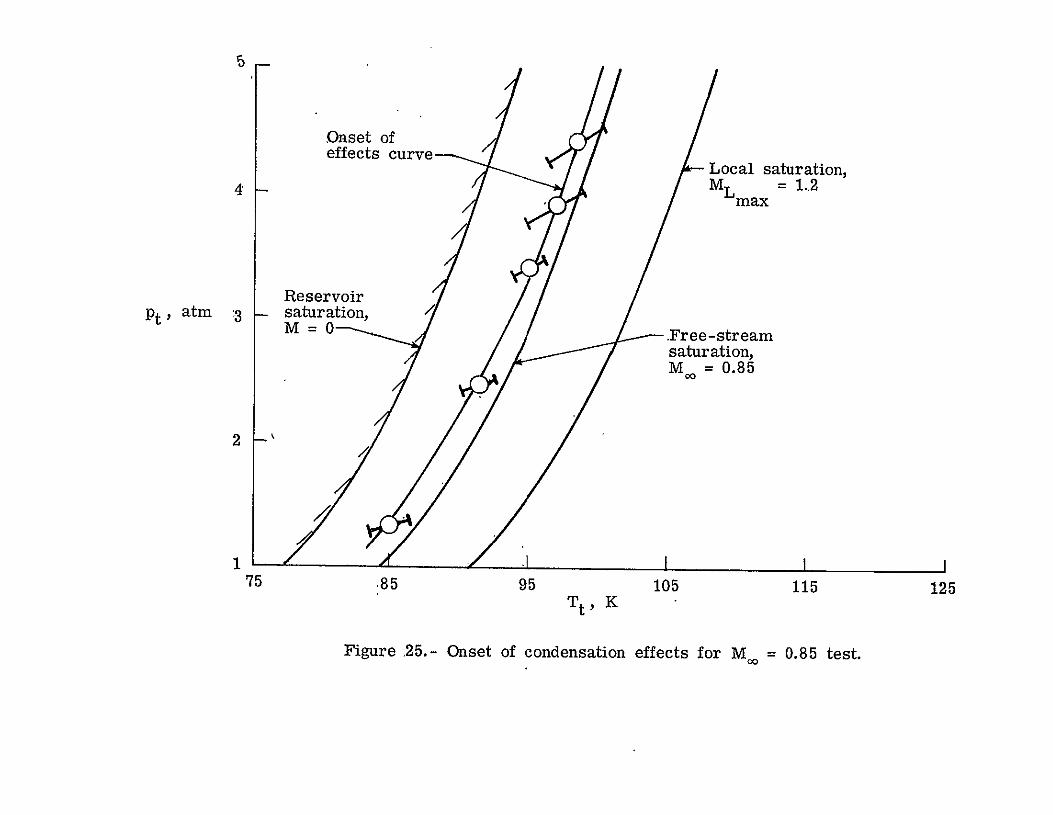
Onset of effects curve

Local saturation, 4 - MLmax

Reservoir pt atm -3 - saturation,

M 0 Free-stream saturation, mo= 0.85

2

75 .85 95 105 115 125 Tt , K

Figure 25.- Onset of condensation effects for M = 0.85 test.

Cp

-. 6

-. 4

-. 2

0

-

-

0 000

0 00 000

0

0 000

0

.2

.4

2 Bad orifice

t

Cl

1.2 0

Figure 26.-

I I 1 I I I I.2 .4 .6 .8

x/c

Average unaffected pressure distribution for

R c = 16 x 106 path of the M, = 0.95 test.

1.0

the

-. 4 -. 0000

0 00

Cp

.2

0

.4

1.2 ;

0

Figure 27.-

0 Bad ,orifice

II I 1J II

.2 x/c .6 .8 .

Average unaffected pressure distribution for the c = 27 x 106 path of the M. = 0.,9'5 test.

-. 8

-.6 -000 0

000~ 0

-. 6 0

0 00 0 00

Cp 0 EO'G o

.2

.4 O]Bad orifice

1.21 0 .2 .4 x/c .6 .8 1.0

Figure 28.- Average unaffected pressure distribution for the Rc = 40 x 106 path of the M. = 0.95 test. (Mi, = 0.93 for this path.)

Local sat Tt 100.4 Onset 0 94 M , sat Tt 89.4 No onset detepted Q

Reservoir sat Tt 78.8 Excessive spatter A

92 Data Min --- Tt 80.0 Bad orifice

Airfoil onset 90­

88 0 000 0 0" 0

Orifice 86 onset TtK 84 '0

82

80 - 0

78 1 I I I I I I 0 .20 .40 .60 :80 1.0.0

Figure 29.- Orifice onset Tt 's and resulting airfoil onset Tt for the

R c = 16 x 106 path of the M,0 = 0.95 test.

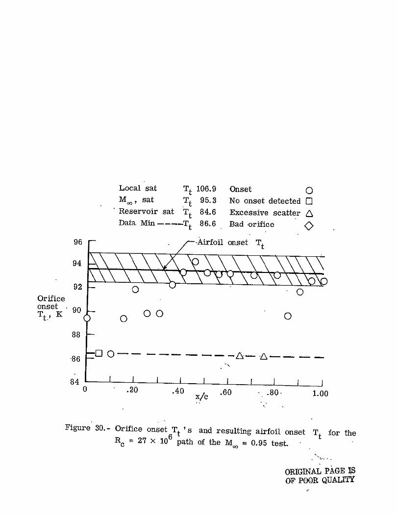
Local sat Tt 106.9 Onset 0 Mm, sat Tt 95.3 No onset detected [ Reservoir sat Tt 84.6 Excessive scatter A Data Min .... Tt 86.6 Bad orifice

96 7 -Airfoil onset Tt

94

92 0

Orifice onset 90 Tt, K 0 00 0

88

086-­

84 0 .20 .40 .60 - .80- 1.00

x/c

Figure 30.- Orifice onset Tt ' s and resulting airfoil onset Tt for the Re = 27 x 106 path of the Mo = 0.95 test.

ORIGINAL PAGE IS OF POOR QUALITY

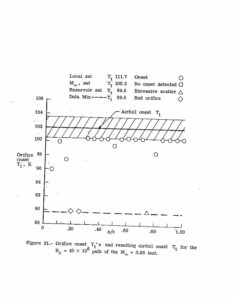
Local sat Tt 111.7 Onset 0 Moo, sat Tt 100.3 No onset detected E0 Reservoir sat Tt 89.8 Excessive scatter /

106 - Data Min-...Tt 89.8 Bad orifice

104 - Airfoil onset Tt

102

100 0

Orifice 98 onset 0 Tt, K

94

92

90 -­

880

I I I .20

1 1 .40 x/c

1 .60

1 1 .80

1 1.00

Figure 31.- Orifice onset Tt's and resulting airfoil onset Tt for the Rc =40 x 106 path of the M. = 0.95 test.

.03 0 SaSat stages x/c = .95 R FS L

.02 OCC,

Error

abar .01 %

0 900CACp

0 0

-. 01

-. 02

70 80, 90 100 110 120 130 Tt, K

Figure 32.- AC vs. T for M 0.93 and R 39.8 million. p w

Unaffected average value of C --'-0.035. P

ORIGINAL PAGE IS OF POOR QUALITY

15-

Local saturation,MLmax = 1.35

4

Onset of effects Free-stream

saturation, = 0.93

Pt atm 3

Reservoir saturation, M=

2

Local saturation

Mmax 13

Free-stream saturation, Moo = 0.95

75 85 95

TtIK 105 115 125

Figure 33.- Onset of condensation effects for the M = 0.95 test.

16 ­

14

'12

10

AT, K 8

i6

4

0 0.75 2 [ 0.85 ORIGINAL PAGRJS

" POOR QUAUT A 0.95

I I I - -]

0 1 2 3 4 5

Pt P atm (a) Supercooling based on MLmax

Figure 34.- Supercooling for all M. tests.

6

4 a

AT, K

0

A 8 gp 2 ,. *'

Moc

0 0.75 0[ 0.85 - 0.95

-4

0

- I I I

1 2 3 4 Pt 'atm

(b) Supercooling based on M.c

FiLure 34.- Concluded.

I

5

10

OA[ 0 M. test Symbol

LoglO p, 0 atm' 0

A 0

0 70

0.85 C3

00 • 0.95 A

A 'Vapor. pressure curve.

-1

60 65 70 '75 80 85 90 T,K

(a) Static values based on M = ML maxFigure 35.- Static values of p, T at onset.

LOglo Pg

atm 0 Vapor pressure curve

mM test

0.75 0.85 0.95

-1 i I i I. I

60- 65 70 75 80 85 90

T,K

(b) Static values based on M =Moo

Figure 35.- Concluded.

Symbol

0 0 A

111 Curve fit to Sivier' s onset

Log 1 0 P, Vapor pressure curve

atm0

0 Mo. test Symbol

0.75 0.85

I0[]

0.95 /

60 65 70 75 80 85 90

T, K

Figure 36.- Data compared with curve fit to Siver's analytically determined onset condltioh .

-0 0

[] 0

Logl0 p,

atm

0

A

0

0 V pressure curve

-1

60

0

I

65

Figure 37.-

I

70

Data compared

Test Symbol

0.75 0 0.85 0 0.95 A

Goglia' s

II

75 80 85

T, K

to dogfia' s data from reference 18.

90

20

12 A

% Increase inR

8 I 4 0

Moo 0.75

El 0.85 A0.95

i I I I 1

0 1 2 Pt

3 4 5 atm

Figure 38.- Percent increase in Reynolds number capability at onset.

26 -

24

20

-

{ 16 -

% Decrease . in power 12 -

8 M 0 0.75 nl 0.85

4 A 0.95

ORIOII M

0 3 2 Pt ) atm

3 atm-4 4 5 OF pooRQtL

Figure 39.- Percent decrease in drive fan power at onset.

20 -

16

.Figure 40.-

Mc,

4 r-10.85

A 0.95

I i I

0 1 2 3 Pt I atm

Percent decrease in LN2 required fan heat.

to

i - i

4 5

absorb drive

1.22 x/c = 0

Cp

1.21

1.20

0

0

0 0 0 000

0*00 0

0 1.19,

0

1.18 .84

Figure 41.- Examples of

00 00 00

1 I0

.85 .86 M

(a) r = 0.15.

curve fits and resulting

0

.87

correlation coefficient, r.

ORIGINAP, 'pAGE IS

OF pOOR QUALiTY'

-. 49 x/c = 0.40

-. 50

0

cp

0 0

-. 52 .84

0 ~0 0

00 0 I

.85 .86 Mo

(b) r = 0.49. Figure 41.- Continued.

.87

-. 02 0­

-. 03

-. 04

-

0

0

00

0

0

-.06

-.07 .84

00 I I

.85 .86 M

(c) r = 0.92. Figure 41.- Concluded.

I .87

OF. POOR

x/c= .80Sat stages.03 LFSR

0.02

0 .01 0

CoAC 0 OO0

O0 -.00

-.02 - o 0

90 100 -110 120 130 70 80

Tt,) K. " ..

(a) Before Mach correction.

of tAp vs. T4ith Mach Figure 42.- Improvement in graphs

= 16 million.correction £or'M = 0.85 and R -0.042.Unaffected average value of Cp

ORIGINAL PAGE IS OF POOR QUALITY

.03-

R

Sat stages

FS L

x/c = .80

.02 i

AC

.01 -

00

nsetO F0

0

of effects

0 0 0 o0

Error bar

-. 01 D 0

-. 02­

0

-. 03 70 80 90 100

Tt, K

10 120 130

(b) After Mach correction.

Figure 42.- Concluded.

1 Report No. 2. Government Accession No. 3. Recipient's Catalog No.

NASA TM 78666 4. Title and Subtitle 5. Report Date

ONSET OF CONDENSATION EFFECTS WITH A NACA 0012-64 March 1978

AIRFOIL TESTED IN THE LANGLEY 0 .3-1ETER CRYOGENIC 6 Performing Organization Code

TUNNEL 3850

7 Author(s) 8 Performing Organization Repbrt No.

Robert M. Hall

IO- Work Unit No.

9. Performing Organization Name and Address

NASA Langley Research Center 11 Contract or Grant No.

Hampton, Virginia 23665

13. Type of Report and Period Covered

12. Sponsoring Agency Name and Address Technical Memorandum National Aeronautics and Space Administration

14 Sponsoring Agency CodeWashington, DC 20546

15 Supplementary Notes

Material will be converted to a formal publication by January 1979.

16. Abstract

A 0.137-m NACA 0012-64 airfoil has been tested in the Langley 0.3-m transonic

cryogenic tunnel at free-stream Mach numbers of 0.75, 0.85, and 0.95 over a total

pressure range from 1.2 to 5.0 atmospheres. The onset of condensation effects were found to correlate more with the amount of supercooling in the free-stream

than it did with the supercooling in the region of maximum local Mach number

over the airfoil. Effects in the pressure distribution over the airfoil were generally seen to appear over its entire length at nearly the same total temperature. Both observations suggest the possibility of heterogeneous

nucleation occurring in the free-stream. Comparisons of the present onset

results are made to calculations by Sivier and data by Goglia. The potential

operational benefits of the supercooling realized are then presented in terms

of increased Reynolds number capability at a given tunnel total pressure,

reduced drive fan power if Reynolds number is held constant, and reduced

liquid nitrogen consumption if Reynolds number is again constant. Depending

on total pressure and free-stream Mach number, these three benefits are

found to,respectively, vary from 7 to 19 percent, 11 to 25 percent, and 9 to

20 percent.

IT Key Words (Suggested by Author(s)) 18 Distribution Statement -

Cryogenic Wind Tunnels Unclassified - Unlimited

Condensation Supercooling Star Category - 02

19. Security Clasif (of this report 20. Security Classif. (of this page) 21. No. of Pages 22. Price*

UUnclassified I 84 $5.00

* For sale by the National Technical Information Service. Springfield. Virginia 22161