NISP Toolbox Manual - Scilabforge.scilab.org/upload/nisp/files/nisp_toolbox_manual... · 2012-02-08 · "Open-Source Platform for Uncertainty treatments in Simulation", funded by

NISP Toolbox Manual

Michael Baudin (INRIA)Jean-Marc Martinez (CEA)

Version 0.3January 2011

Abstract

This document is an introduction to the NISP module. We present the installation process of themodule in binary from ATOMS or from the sources. Then we present the configuration functionsand the randvar, setrandvar and polychaos classes. Several examples are provided for eachclass, which provides an overview of the use of NISP in practical situations.

Contents

1 Introduction 41.1 The OPUS project . . . . . . . . . . . . . . . . . . . . . . . . . . . . . . . . . . . 41.2 The NISP library . . . . . . . . . . . . . . . . . . . . . . . . . . . . . . . . . . . . 41.3 The NISP module . . . . . . . . . . . . . . . . . . . . . . . . . . . . . . . . . . . . 5

2 Installation 102.1 Introduction . . . . . . . . . . . . . . . . . . . . . . . . . . . . . . . . . . . . . . . 102.2 Installing the toolbox from ATOMS . . . . . . . . . . . . . . . . . . . . . . . . . . 112.3 Installing the toolbox from the sources . . . . . . . . . . . . . . . . . . . . . . . . 12

3 Configuration functions 17

4 The randvar class 184.1 The distribution functions . . . . . . . . . . . . . . . . . . . . . . . . . . . . . . . 18

4.1.1 Overview . . . . . . . . . . . . . . . . . . . . . . . . . . . . . . . . . . . . 184.1.2 Parameters of the Log-normal distribution . . . . . . . . . . . . . . . . . . 194.1.3 Uniform random number generation . . . . . . . . . . . . . . . . . . . . . . 19

4.2 Methods . . . . . . . . . . . . . . . . . . . . . . . . . . . . . . . . . . . . . . . . . 204.2.1 Overview . . . . . . . . . . . . . . . . . . . . . . . . . . . . . . . . . . . . 204.2.2 The Oriented-Object system . . . . . . . . . . . . . . . . . . . . . . . . . . 20

4.3 Examples . . . . . . . . . . . . . . . . . . . . . . . . . . . . . . . . . . . . . . . . 224.3.1 A sample session . . . . . . . . . . . . . . . . . . . . . . . . . . . . . . . . 234.3.2 Variable transformations . . . . . . . . . . . . . . . . . . . . . . . . . . . . 23

5 The setrandvar class 285.1 Introduction . . . . . . . . . . . . . . . . . . . . . . . . . . . . . . . . . . . . . . . 285.2 Examples . . . . . . . . . . . . . . . . . . . . . . . . . . . . . . . . . . . . . . . . 28

5.2.1 A Monte-Carlo design with 2 variables . . . . . . . . . . . . . . . . . . . . 285.2.2 A Monte-Carlo design with 2 variables . . . . . . . . . . . . . . . . . . . . 325.2.3 A LHS design . . . . . . . . . . . . . . . . . . . . . . . . . . . . . . . . . . 345.2.4 A note on the LHS samplings . . . . . . . . . . . . . . . . . . . . . . . . . 385.2.5 Other types of DOEs . . . . . . . . . . . . . . . . . . . . . . . . . . . . . . 41

6 The polychaos class 456.1 Introduction . . . . . . . . . . . . . . . . . . . . . . . . . . . . . . . . . . . . . . . 456.2 Examples . . . . . . . . . . . . . . . . . . . . . . . . . . . . . . . . . . . . . . . . 45

6.2.1 Product of two random variables . . . . . . . . . . . . . . . . . . . . . . . 45

1

6.2.2 A note on performance . . . . . . . . . . . . . . . . . . . . . . . . . . . . . 506.2.3 The Ishigami test case . . . . . . . . . . . . . . . . . . . . . . . . . . . . . 52

7 Thanks 56

Bibliography 57

2

Copyright c© 2008-2011 - INRIA - Michael BaudinCopyright c© 2008-2011 - CEA - Jean-Marc MartinezCopyright c© 2012 - Michael BaudinThis file must be used under the terms of the Creative Commons Attribution-ShareAlike 3.0

Unported License:

http://creativecommons.org/licenses/by-sa/3.0

3

http://creativecommons.org/licenses/by-sa/3.0

Chapter 1

Introduction

1.1 The OPUS project

The goal of this toolbox is to provide a tool to manage uncertainties in simulated models. Thistoolbox is based on the NISP library, where NISP stands for ”Non-Intrusive Spectral Projection”.This work has been realized in the context of the OPUS project,

http://opus-project.fr

”Open-Source Platform for Uncertainty treatments in Simulation”, funded by ANR, the french”Agence Nationale pour la Recherche”:

http://www.agence-nationale-recherche.fr

The toolbox is released under the Lesser General Public Licence (LGPL), as all components ofthe OPUS project.

This module was presented in the ”42emes Journees de Statistique, du 24 au 28 mai 2010” [2].

1.2 The NISP library

The NISP library is based on a set of 3 C++ classes so that it provides an object-orientedframework for uncertainty analysis. The Scilab toolbox provides a pseudo-object oriented interfaceto this library, so that the two approaches are consistent. The NISP library is release under theLGPL licence.

The NISP library provides three tools, which are detailed below.

• The ”randvar” class allows to manage random variables, specified by their distribution lawand their parameters. Once a random variable is created, one can generate random numbersfrom the associated law.

• The ”setrandvar” class allows to manage a collection of random variables. This collectionis associated with a sampling method, such as MonteCarlo, Sobol, Quadrature, etc... It ispossible to build the sample and to get it back so that the experiments can be performed.

• The ”polychaos” class allows to manage a polynomial representation of the simulated model.One such object must be associated with a set of experiments which have been performed.

4

http://opus-project.fr

http://www.agence-nationale-recherche.fr

This set may be read from a data file. The object is linked with a collection of randomvariables. Then the coefficients of the polynomial can be computed by integration (quadra-ture). Once done, the mean, the variance and the Sobol indices can be directly computedfrom the coefficients.

The figure 1.1 presents the NISP methodology. The process requires that the user has anumerical solver, which has the form Y = f(X), where X are input uncertain parameters and Yare output random variables. The method is based on the following steps.

• We begin by defining normalized random variables ξ. For example, we may use a randomvariables in the interval [0, 1] or a Normal random variable with mean 0 and variance 1. Thischoice allows to define the basis for the polynomial chaos, denoted by {Ψk}k≥0. Dependingon the type of random variable, the polynomials {Ψk}k≥0 are based on Hermite, Legendreor Laguerre polynomials.

• We can now define a Design Of Experiments (DOE) and, with random variable transforma-tions rules, we get the physical uncertain parameters X. Several types of DOE are available:Monte-Carlo, Latin Hypercube Sampling, etc... If N experiments are required, the DOEdefine the collection of normalized random variables {ξi}i=1,N . Transformation rules allowsto compute the uncertain parameters {Xi}i=1,N , which are the input of the numerical solverf .

• We can now perform the simulations, that is compute the collection of outputs {Yi}i=1,N

where Yi = f(Xi).

• The variables Y are then projected on the polynomial basis and the coefficients yk arecomputed by integration or regression.

RandomVariable ξ

UncertainParameter X

NumericalSolver Y=f(X)

SpectralProjectionY = Σ y ψ(ξ)

Figure 1.1: The NISP methodology

1.3 The NISP module

The NISP toolbox is available under the following operating systems:

• Linux 32 bits,

• Linux 64 bits,

• Windows 32 bits,

• Mac OS X.

5

The following list presents the features provided by the NISP toolbox.

• Manage various types of random variables:

– uniform,

– normal,

– exponential,

– log-normal.

• Generate random numbers from a given random variable,

• Transform an outcome from a given random variable into another,

• Manage various Design of Experiments for sets of random variables,

– Monte-Carlo,

– Sobol,

– Latin Hypercube Sampling,

– various samplings based on Smolyak designs.

• Manage polynomial chaos expansion and get specific outputs, including

– mean,

– variance,

– quantile,

– correlation,

– etc...

• Generate the C source code which computes the output of the polynomial chaos expansion.

This User’s Manual completes the online help provided with the toolbox, but does not replaceit. The goal of this document is to provide both a global overview of the toolbox and to give somedetails about its implementation. The detailed calling sequence of each function is provided bythe online help and will not be reproduced in this document. The inline help is presented in thefigure 1.2.

For example, in order to access to the help associated with the randvar class, we type thefollowing statements in the Scilab console.

help randvar

The previous statements opens the Help Browser and displays the helps page presented in figureSeveral demonstration scripts are provided with the toolbox and are presented in the figure

1.4. These demonstrations are available under the ”?” question mark in the menu of the Scilabconsole.

Finally, the unit tests provided with the toolbox cover all the features of the toolbox. Whenwe want to know how to use a particular feature and do not find the information, we can searchin the unit tests which often provide the answer.

6

Figure 1.2: The NISP inline help.

7

Figure 1.3: The online help of the randvar function.

8

Figure 1.4: Demonstrations provided with the NISP toolbox.

9

Chapter 2

Installation

In this section, we present the installation process for the toolbox. We present the steps whichare required to have a running version of the toolbox and presents the several checks which canbe performed before using the toolbox.

2.1 Introduction

There are two possible ways of installing the NISP toolbox in Scilab:

• use the ATOMS system and get a binary version of the toolbox,

• build the toolbox from the sources.

The next two sections present these two ways of using the toolbox.Before getting into the installation process, let us present some details of the the internal

components of the toolbox. The following list is an overview of the content of the directories:

• tbxnisp/demos : demonstration scripts

• tbxnisp/doc : the documentation

• tbxnisp/doc/usermanual : the LATEXsources of this manual

• tbxnisp/etc : startup and shutdow scripts for the toolbox

• tbxnisp/help : inline help pages

• tbxnisp/macros : Scilab macros files *.sci

• tbxnisp/sci gateway : the sources of the gateway

• tbxnisp/src : the sources of the NISP library

• tbxnisp/tests : tests

• tbxnisp/tests/nonreg tests : tests after some bug has been identified

• tbxnisp/tests/unit tests : unit tests

The current version is based on the NISP Library v2.1.

10

2.2 Installing the toolbox from ATOMS

The ATOMS component is the Scilab tool which allows to search, download, install and loadtoolboxes. ATOMS comes with Scilab v5.2. The Scilab-NISP toolbox has been packaged and isprovided mainly by the ATOMS component. The toolbox is provided in binary form, dependingon the user’s operating system. The Scilab-NISP toolbox is available for the following platforms:

• Windows 32 bits,

• Linux 32 bits, 64 bits,

• Mac OS X.

The ATOMS component allows to use a toolbox based on compiled source code, without havinga compiler installed in the system.

Installing the Scilab-NISP toolbox from ATOMS requires the following steps:

• atomsList(): prints the list of current toolboxes,

• atomsShow(): prints informations about a toolbox,

• atomsInstall(): installs a toolbox on the system,

• atomsLoad(): loads a toolbox.

Once installed and loaded, the toolbox will be available on the system from session to session, sothat there is no need to load the toolbox again: it will be available right from the start of thesession.

In the following Scilab session, we use the atomsList() function to print the list of all ATOMStoolboxes.

--> atomsList ()

ANN_Toolbox - ANN Toolbox

dde_toolbox - Dynamic Data Exchange client for Scilab

module_lycee - Scilab pour les lyc~Al’es

NISP - Non Intrusive Spectral Projection

plotlib - "Matlab -like" Plotting library for Scilab

scipad - Scipad 7.20

sndfile_toolbox - Read & write sound files

stixbox - Statistics toolbox for Scilab 5.2

In the following Scilab session, we use the atomsShow() function to print the details aboutthe NISP toolbox.

-->atomsShow ("NISP")

Package : NISP

Title : NISP

Summary : Non Intrusive Spectral Projection

Version : 2.1

Depend : Category(ies) : Optimization

Maintainer(s) : Pierre Marechal <[email protected] >

Michael Baudin <[email protected] >

11

Entity : CEA / DIGITEO

WebSite : License : LGPL

Scilab Version : >= 5.2.0

Status : Not installed

Description : This toolbox allows to approximate a given model ,

which is associated with input random variables.

This toolbox has been created in the context of the

OPUS project :

http ://opus -project.fr/

within the workpackage 2.1.1:

"Construction de m~Al’ta-mod~Alles"

This project has received funding by Agence Nationale

de la recherche :

http :// www.agence -nationale -recherche.fr/

See in the help provided in the help/en_US directory

of the toolbox for more information about its use.

Use cases are presented in the demos directory.

In the following Scilab session, we use the atomsInstall() function to download and installthe binary version of the toolbox corresponding to the current operating system.

-->atomsInstall ( "NISP" )

ans =

!NISP 2.1 allusers D:\ Programs\SC3623 ~1\ contrib\NISP \2.1 I !

The "allusers" option of the atomsInstall function can be used to install the toolbox for allthe users of this computer. We finally load the toolbox with the atomsLoad() function.

-->atomsLoad ("NISP")

Start NISP Toolbox

Load gateways

Load help

Load demos

ans =

!NISP 2.1 D:\ Programs\SC3623 ~1\ contrib\NISP \2.1 !

Now that the toolbox is loaded, it will be automatically loaded at the next Scilab session.

2.3 Installing the toolbox from the sources

In this section, we present the steps which are required in order to install the toolbox from thesources.

In order to install the toolbox from the sources, a compiler is required to be installed on themachine. This toolbox can be used with Scilab v5.1 and Scilab v5.2. We suppose that the archivehas been unpacked in the ”tbxnisp” directory. The following is a short list of the steps which arerequired to setup the toolbox.

1. build the toolbox : run the tbxnisp/builder.sce script to create the binaries of the library,create the binaries for the gateway, generate the documentation

2. load the toolbox : run the tbxnisp/load.sce script to load all commands and setup thedocumentation

12

3. setup the startup configuration file of your Scilab system so that the toolbox is known atstartup (see below for details),

4. run the unit tests : run the tbxnisp/runtests.sce script to perform all unit tests and checkthat the toolbox is OK

5. run the demos : run the tbxnisp/rundemos.sce script to run all demonstration scripts andget a quick interactive overview of its features

The following script presents the messages which are generated when the builder of the toolboxis launched. The builder script performs the following steps:

• compile the NISP C++ library,

• compile the C++ gateway library (the glue between the library and Scilab),

• generate the Java help files from the .xml files,

• generate the loader script.

-->exec C:\ tbxnisp\builder.sce;

Building sources ...

Generate a loader file

Generate a Makefile

Running the Makefile

Compilation of utils.cpp

Compilation of blas1_d.cpp

Compilation of dcdflib.cpp

Compilation of faure.cpp

Compilation of halton.cpp

Compilation of linpack_d.cpp

Compilation of niederreiter.cpp

Compilation of reversehalton.cpp

Compilation of sobol.cpp

Building shared library (be patient)

Generate a cleaner file


Generate a Makefile

Running the Makefile

Compilation of nisp_gc.cpp

Compilation of nisp_gva.cpp

Compilation of nisp_ind.cpp

Compilation of nisp_index.cpp

Compilation of nisp_inv.cpp

Compilation of nisp_math.cpp

Compilation of nisp_msg.cpp

Compilation of nisp_conf.cpp

Compilation of nisp_ort.cpp

Compilation of nisp_pc.cpp

Compilation of nisp_polyrule.cpp

13

Compilation of nisp_qua.cpp

Compilation of nisp_random.cpp

Compilation of nisp_smo.cpp

Compilation of nisp_util.cpp

Compilation of nisp_va.cpp

Compilation of nisp_smolyak.cpp



Building gateway ...

Generate a gateway file


Generate a Makefile: Makelib

Running the makefile

Compilation of nisp_gettoken.cpp

Compilation of nisp_gwsupport.cpp

Compilation of nisp_PolynomialChaos_map.cpp

Compilation of nisp_RandomVariable_map.cpp

Compilation of nisp_SetRandomVariable_map.cpp

Compilation of sci_nisp_startup.cpp

Compilation of sci_nisp_shutdown.cpp

Compilation of sci_nisp_verboselevelset.cpp

Compilation of sci_nisp_verboselevelget.cpp

Compilation of sci_nisp_initseed.cpp

Compilation of sci_randvar_new.cpp

Compilation of sci_randvar_destroy.cpp

Compilation of sci_randvar_size.cpp

Compilation of sci_randvar_tokens.cpp

Compilation of sci_randvar_getlog.cpp

Compilation of sci_randvar_getvalue.cpp

Compilation of sci_setrandvar_new.cpp

Compilation of sci_setrandvar_tokens.cpp

Compilation of sci_setrandvar_size.cpp

Compilation of sci_setrandvar_destroy.cpp

Compilation of sci_setrandvar_freememory.cpp

Compilation of sci_setrandvar_addrandvar.cpp

Compilation of sci_setrandvar_getlog.cpp

Compilation of sci_setrandvar_getdimension.cpp

Compilation of sci_setrandvar_getsize.cpp

Compilation of sci_setrandvar_getsample.cpp

Compilation of sci_setrandvar_setsample.cpp

Compilation of sci_setrandvar_save.cpp

Compilation of sci_setrandvar_buildsample.cpp

Compilation of sci_polychaos_new.cpp

Compilation of sci_polychaos_destroy.cpp

Compilation of sci_polychaos_tokens.cpp

Compilation of sci_polychaos_size.cpp

Compilation of sci_polychaos_setdegree.cpp

Compilation of sci_polychaos_getdegree.cpp

Compilation of sci_polychaos_freememory.cpp

14

Compilation of sci_polychaos_getdimoutput.cpp

Compilation of sci_polychaos_setdimoutput.cpp

Compilation of sci_polychaos_getsizetarget.cpp

Compilation of sci_polychaos_setsizetarget.cpp

Compilation of sci_polychaos_freememtarget.cpp

Compilation of sci_polychaos_settarget.cpp

Compilation of sci_polychaos_gettarget.cpp

Compilation of sci_polychaos_getdiminput.cpp

Compilation of sci_polychaos_getdimexp.cpp

Compilation of sci_polychaos_getlog.cpp

Compilation of sci_polychaos_computeexp.cpp

Compilation of sci_polychaos_getmean.cpp

Compilation of sci_polychaos_getvariance.cpp

Compilation of sci_polychaos_getcovariance.cpp

Compilation of sci_polychaos_getcorrelation.cpp

Compilation of sci_polychaos_getindexfirst.cpp

Compilation of sci_polychaos_getindextotal.cpp

Compilation of sci_polychaos_getmultind.cpp

Compilation of sci_polychaos_getgroupind.cpp

Compilation of sci_polychaos_setgroupempty.cpp

Compilation of sci_polychaos_getgroupinter.cpp

Compilation of sci_polychaos_getinvquantile.cpp

Compilation of sci_polychaos_buildsample.cpp

Compilation of sci_polychaos_getoutput.cpp

Compilation of sci_polychaos_getquantile.cpp

Compilation of sci_polychaos_getquantwilks.cpp

Compilation of sci_polychaos_getsample.cpp

Compilation of sci_polychaos_setgroupaddvar.cpp

Compilation of sci_polychaos_computeoutput.cpp

Compilation of sci_polychaos_setinput.cpp

Compilation of sci_polychaos_propagateinput.cpp

Compilation of sci_polychaos_getanova.cpp

Compilation of sci_polychaos_setanova.cpp

Compilation of sci_polychaos_getanovaord.cpp

Compilation of sci_polychaos_getanovaordco.cpp

Compilation of sci_polychaos_realisation.cpp

Compilation of sci_polychaos_save.cpp

Compilation of sci_polychaos_generatecode.cpp



Generating loader_gateway.sce...

Building help ...

Building the master document:

C:\ tbxnisp\help\en_US

Building the manual file [javaHelp] in

C:\ tbxnisp\help\en_US.

(Please wait building ... this can take a while)

Generating loader.sce...

The following script presents the messages which are generated when the loader of the toolbox

15

is launched. The loader script performs the following steps:

• load the gateway (and the NISP library),

• load the help,

• load the demo.

-->exec C:\ tbxnisp\loader.sce;

Start NISP Toolbox

Load gateways

Load help

Load demos

It is now necessary to setup your Scilab system so that the toolbox is loaded automaticallyat startup. The way to do this is to configure the Scilab startup configuration file. The directorywhere this file is located is stored in the Scilab variable SCIHOME. In the following Scilab session,we use Scilab v5.2.0-beta-1 in order to know the value of the SCIHOME global variable.

-->SCIHOME

SCIHOME =

C:\Users\baudin\AppData\Roaming\Scilab\scilab -5.2.0 -beta -1

On my Linux system, the Scilab 5.1 startup file is located in

/home/myname/.Scilab/scilab-5.1/.scilab.

On my Windows system, the Scilab 5.1 startup file is located in

C:/Users/myname/AppData/Roaming/Scilab/scilab-5.1/.scilab.

This file is a regular Scilab script which is automatically loaded at Scilab’s startup. If that filedoes not already exist, create it. Copy the following lines into the .scilab file and configure thepath to the toolboxes, stored in the SCILABTBX variable.

exec("C:\ tbxnisp\loader.sce");

The following script presents the messages which are generated when the unit tests script ofthe toolbox is launched.

-->exec C:\ tbxnisp\runtests.sce;

Tests beginning the 2009/11/18 at 12:47:45

TMPDIR = C:\Users\baudin\AppData\Local\Temp\SCI_TMP_6372_

001/004 - [tbxnisp] nisp .................. passed : ref created

002/004 - [tbxnisp] polychaos1 ............ passed : ref created

003/004 - [tbxnisp] randvar1 .............. passed : ref created

004/004 - [tbxnisp] setrandvar1 ........... passed : ref created

--------------------------------------------------------------

Summary

tests 4 - 100 %

passed 0 - 0 %

failed 0 - 0 %

skipped 0 - 0 %

length 3.84 sec

--------------------------------------------------------------

Tests ending the 2009/11/18 at 12:47:48\ end{verbatim}

16

Chapter 3

Configuration functions

In this section, we present functions which allow to configure the NISP toolbox.The nisp_* functions allows to configure the global behaviour of the toolbox. These func-

tions allows to startup and shutdown the toolbox and initialize the seed of the random numbergenerator. They are presented in the figure 3.1.

nisp_startup () Starts up the NISP toolbox.nisp_shutdown () Shuts down the NISP toolbox.level = nisp_verboselevelget () Returns the current verbose level.nisp_verboselevelset ( level ) Sets the value of the verbose level.nisp_initseed ( seed ) Sets the seed of the uniform

random number generator.nisp_destroyall Destroy all current objects.nisp_getpath Returns the path to the current module.nisp_printall Prints all current objects.

Figure 3.1: Outline of the configuration methods.

The user has no need to explicitely call the nisp_startup () and nisp_shutdown () func-tions. Indeed, these functions are called automatically by the etc/NISP.start and etc/NISP.quitscripts, located in the toolbox directory structure.

The nisp_initseed ( seed ) is especially useful when we want to have reproductible re-sults. It allows to set the seed of the generator at a particular value, so that the sequence ofuniform pseudo-random numbers is deterministic. When the toolbox is started up, the seed isautomatically set to 0, which allows to get the same results from session to session.

17

Chapter 4

The randvar class

In this section, we present the randvar class, which allows to define a random variable, and togenerate random numbers from a given distribution function.

4.1 The distribution functions

In this section, we present the distribution functions provided by the randvar class. We especiallypresent the Log-normal distribution function.

4.1.1 Overview

The table 4.1 gives the list of distribution functions which are available with the randvar class[3].

Each distribution functions have zero, one or two parameters. One random variable can bespecified by giving explicitely its parameters or by using default parameters. The parameters forall distribution function are presented in the figure 4.2, which also presents the conditions whichmust be satisfied by the parameters.

Name f(x) E(X) V (X)

”Normale” 12σ√2π

exp(− 1

2(x−µ)2σ2

)µ σ2

”Uniforme”

{1b−a , if x ∈ [a, b[

0 if x /∈ [a, b[b+a2

(b−a)212

”Exponentielle”

{λ exp (−λx) , if x > 00 if x ≤ 0

1λ

1λ2

”LogNormale”

{1

σx√2π

exp(− 1

2(ln(x)−µ)2

σ2

), if x > 0

0 if x ≤ 0exp

(µ+ 1

2σ2) (

exp(σ2)− 1)exp

(2µ+ σ2

)”LogUniforme”

{ 1x

1ln(b)−ln(a) , if x ∈ [a, b[

0 if x /∈ [a, b[b−a

ln(b)−ln(a)12

b2−a2ln(b)−ln(a) − E(x)

Figure 4.1: Distributions functions of the randvar class. – The expected value is denoted byE(X) and the variance is denoted by V (X).

18

Name Parameter #1 : a Parameter #2 : b Conditions”Normale” µ = 0. σ = 1. σ > 0”Uniforme” a = 0. b = 1. a < b”Exponentielle” λ = 1. - -”LogNormale” µ′ = 0.1 σ = 1.0 µ′, σ > 0”LogUniforme” a = 0.1 b = 1.0 a, b > 0, a < b

Figure 4.2: Default parameters for distributions functions.

4.1.2 Parameters of the Log-normal distribution

A log-normal distribution is a probability distribution of a random variable whose logarithm isnormally distributed. If X is a random variable with a normal distribution, then Y = exp(X)has a log-normal distribution.

For the ”LogNormale” law, the distribution function is usually defined by the expected valueµ and the standard deviation σ of the underlying Normal random variable. But, when we createa LogNormale randvar, the parameters to pass to the constructor are the expected value of theLogNormal random variable E(X) and the standard deviation of the underlying Normale randomvariable σ. The expected value and the variance of the Log Normal law are given by

E(X) = exp

(µ+

1

2σ2

)(4.1)

V (X) =(exp(σ2)− 1

)exp

(2µ+ σ2

). (4.2)

In the figure 4.2, we have µ′ = E(X).It is possible to invert these formulas, in the situation where the given parameters are the

expected value and the variance of the Log Normal random variable. We can invert completelythe previous equations and get

µ = ln(E(X))− 1

2ln

(1 +

V (X)

E(X)2

)(4.3)

σ2 = ln

(1 +

V (X)

E(X)2

). (4.4)

In particular, the expected value µ of with the Normal random variable satisfies the equation

µ = ln(E(X))− σ2. (4.5)

4.1.3 Uniform random number generation

In this section, we present the generation of uniform random numbers.The goal of this section is to warn users about a current limitation of the library. Indeed, the

random number generator is based on the compiler, so that its quality cannot be guaranted.The Uniforme law is associated with the parameters a, b ∈ R with a < b. It produces real

values uniform in the interval [a, b].To compute the uniform random number X in the interval [a, b], a uniform random number

in the interval [0, 1] is generated and then scaled with

X = a+ (b− a)X. (4.6)

19

Let us now analyse how the uniform random number X ∈ [0, 1] is computed. The uniformrandom generator is based on the C function rand, which returns an integer n in the interval[0, RAND MAX[. The value of the RAND MAX variable is defined in the file stdlib.h and iscompiler-dependent. For example, with the Visual Studio C++ 2008 compiler, the value is

RAND MAX = 215 − 1 = 32767. (4.7)

A uniform value X in the range [0, 1[ is computed from

X =n

N, (4.8)

where N = RAND MAX and n ∈ [0, RAND MAX[.

4.2 Methods

In this section, we give an overview of the methods which are available in the randvar class.

4.2.1 Overview

The figure 4.3 presents the methods available in the randvar class. The inline help contains thedetailed calling sequence for each function and will not be repeated here.

Constructorsrv = randvar_new ( type [, options])

Methodsvalue = randvar_getvalue ( rv [, options] )

randvar_getlog ( rv )

Destructorrandvar_destroy ( rv )

Static methodsrvlist = randvar_tokens ()

nbrv = randvar_size ()

Figure 4.3: Outline of the methods of the randvar class.

4.2.2 The Oriented-Object system

In this section, we present the token system which allows to emulate an oriented-object program-ming with Scilab. We also present the naming convention we used to create the names of thefunctions.

The randvar class provides the following functions.

• The constructor function randvar_new allows to create a new random variable and returnsa token rv.

20

• The method randvar_getvalue takes the token rv as its first argument. In fact, all methodstakes as their first argument the object on which they apply.

• The destructor randvar_destroy allows to delete the current object from the memory ofthe library.

• The static methods randvar_tokens and randvar_size allows to quiery the current objectwhich are in use. More specifically, the randvar_size function returns the number of currentrandvar objects and the randvar_tokens returns the list of current randvar objects.

In the following Scilab sessions, we present these ideas with practical uses of the toolbox.Assume that we start Scilab and that the toolbox is automatically loaded. At startup, there

are no objects, so that the randvar_size function returns 0 and the randvar_tokens functionreturns an empty matrix.

-->nb = randvar_size ()

nb =

0.

-->tokenmatrix = randvar_tokens ()

tokenmatrix =

[]

We now create 3 new random variables, based on the Uniform distribution function. We storethe tokens in the variables vu1, vu2 and vu3. These variables are regular Scilab double precisionfloating point numbers. Each value is a token which represents a random variable stored in thetoolbox memory space.

-->vu1 = randvar_new("Uniforme")

vu1 =

0.


vu2 =

1.


vu3 =

2.

There are now 3 objects in current use, as indicated by the following statements. Thetokenmatrix is a row matrix containing regular double precision floating point numbers.


nb =

3.


tokenmatrix =

0. 1. 2.

We assume that we have now made our job with the random variables, so that it is timeto destroy the random variables. We call the randvar_destroy functions, which destroys thevariables.

-->randvar_destroy(vu1);



21

We can finally check that there are no random variables left in the memory space.


nb =

0.


tokenmatrix =

[]

Scilab is a wonderful tool to experiment algorithms and make simulations. It happens some-times that we are managing many variables at the same time and it may happen that, at somepoint, we are lost. The static methods provides tools to be able to recover from such a situationwithout closing our Scilab session.

In the following session, we create two random variables.


vu1 =

3.


vu2 =

4.

Assume now that we have lost the token associated with the variable vu2. We can easily simulatethis situation, by using the clear, which destroys a variable from Scilab’s memory space.

-->clear vu2

-->randvar_getvalue(vu2)

!--error 4

Undefined variable: vu2

It is now impossible to generate values from the variable vu2. Moreover, it may be difficult toknow exactly what went wrong and what exact variable is lost. At any time, we can use therandvar_tokens function in order to get the list of current variables. Deleting these variablesallows to clean the memory space properly, without memory loss.

-->randvar_tokens ()

ans =

3. 4.

-->randvar_destroy (3)

ans =

3.

-->randvar_destroy (4)

ans =

4.

-->randvar_tokens ()

ans =

[]

4.3 Examples

In this section, we present to examples of use of the randvar class. The first example presentsthe simulation of a Normal random variable and the generation of 1000 random variables. The

22

second example presents the transformation of a Uniform outcome into a LogUniform outcome.

4.3.1 A sample session

We present a sample Scilab session, where the randvar class is used to generate samples from theNormale law.

In the following Scilab session, we create a Normale random variable and compute samplesfrom this law. The nisp_initseed function is used to initialize the seed for the uniform randomvariable generator. Then we use the randvar_new function to create a new random variable fromthe Normale law with mean 1. and standard deviation 0.5. The main loop allows to compute1000 samples from this law, based on calls to the randvar_getvalue function. Once the samplesare computed, we use the Scilab function mean to check that the mean is close to 1 (which isthe expected value of the Normale law, when the number of samples is infinite). Finally, we usethe randvar_destroy function to destroy our random variable. Once done, we plot the empiricaldistribution function of this sample, with 50 classes.

nisp_initseed ( 0 );

mu = 1.0;

sigma = 0.5;

rv = randvar_new("Normale" , mu , sigma);

nbshots = 1000;

values = zeros(nbshots );

for i=1: nbshots

values(i) = randvar_getvalue(rv);

end

mymean = mean (values );

mysigma = st_deviation(values );

myvariance = variance (values );

mprintf("Mean : %f (expected = %f)\n", mymean , mu);

mprintf("Std. dev. : %f (expected = %f)\n", mysigma , sigma);

mprintf("Variance : %f (expected = %f)\n", myvariance , sigma ^2);

randvar_destroy(rv);

histplot (50, values)

xtitle("Histogram of X","X","P(x)")

The previous script produces the following output.

Mean : 0.988194 (expected = 1.000000)

Std. dev. : 0.505186 (expected = 0.500000)

Variance : 0.255213 (expected = 0.250000)

The previous script also produces the figure 4.4.

4.3.2 Variable transformations

In this section, we present the transformation of uniform random variables into other types ofvariables. The transformations which are available in the randvar class are presented in figure4.5. We begin the analysis by a presentation of the theory required to perform transformations.Then we present some of the many the transformations which are provided by the library.

23

0.0

0.1

0.2

0.3

0.4

0.5

0.6

0.7

0.8

0.9

-1.0 -0.5 0.0 0.5 1.0 1.5 2.0 2.5 3.0

Histogram of X

X

P(x

)

Figure 4.4: The histogram of a Normal random variable with 1000 samples.

Source TargetNormale

NormaleUniformeExponentielleLogNormaleLogUniforme

Source TargetLogNormale

NormaleUniformeExponentielleLogNormaleLogUniforme

Source TargetUniforme

UniformeNormaleExponentielleLogNormaleLogUniforme

Source TargetLogUniforme

UniformeNormaleExponentielleLogNormaleLogUniforme

Source TargetExponentielle

Exponentielle

Figure 4.5: Variable transformations available in the randvar class.

24

We now present some additionnal details for the function randvar_getvalue ( rv , rv2 ,

value2 ). This method allows to transform a random variable sample from one law to another.The statement

value = randvar_getvalue ( rv , rv2 , value2 )

returns a random value from the distribution function of the random variable rv by transformationof value2 from the distribution function of random variable rv2.

In the following session, we transform a uniform random variable sample into a LogUniformvariable sample. We begin to create a random variable rv from a LogUniform law and parametersa = 10, b = 20. Then we create a second random variable rv2 from a Uniforme law and parametersa = 2, b = 3. The main loop is based on the transformation of a sample computed from rv2 intoa sample from rv. The mean allows to check that the transformed samples have an mean valuewhich corresponds to the random variable rv.


a = 10.0;

b = 20.0;

rv = randvar_new ( "LogUniforme" , a , b );

rv2 = randvar_new ( "Uniforme" , 2 , 3 );

nbshots = 1000;

valuesLou = zeros(nbshots );

for i=1: nbshots

valuesUni(i) = randvar_getvalue( rv2 );

valuesLou(i) = randvar_getvalue( rv , rv2 , valuesUni(i) );

end

computed = mean (valuesLou );

mu = (b-a)/(log(b)-log(a));

expected = mu;

mprintf("Expectation=%.5f (expected=%.5f)\n",computed ,expected );

//

scf();

histplot (50, valuesUni );

xtitle("Empirical histogram - Uniform variable","X","P(X)");

scf();

histplot (50, valuesLou );

xtitle("Empirical histogram - Log -Uniform variable","X","P(X)");

randvar_destroy(rv);

randvar_destroy(rv2);


Expectation =14.63075 (expected =14.42695)

The previous script also produces the figures 4.6 and 4.7.The transformation depends on the mother random variable rv1 and on the daughter ran-

dom variable rv. Specific transformations are provided for all many combinations of the twodistribution functions. These transformations will be analysed in the next sections.

25

0.0

0.2

0.4

0.6

0.8

1.0

1.2

1.4

1.6

2.0 2.1 2.2 2.3 2.4 2.5 2.6 2.7 2.8 2.9 3.0

Empirical histogram - Uniform variable

X

P(X

)

Figure 4.6: The histogram of a Uniform random variable with 1000 samples.

26

0.00

0.02

0.04

0.06

0.08

0.10

0.12

0.14

0.16

0.18

10 11 12 13 14 15 16 17 18 19 20

Empirical histogram - Log-Uniform variable

X

P(X

)

Figure 4.7: The histogram of a Log-Uniform random variable with 1000 samples.

27

Chapter 5

The setrandvar class

In this chapter, we presen the setrandvar class. The first section gives a brief outline of thefeatures of this class and the second section present several examples.

5.1 Introduction

The setrandvar class allows to manage a collection of random variables and to build a DesignOf Experiments (DOE). Several types of DOE are provided:

• Monte-Carlo,

• Latin Hypercube Sampling,

• Smolyak.

Once a DOE is created, we can retrieve the information experiment by experiment or the wholematrix of experiments. This last feature allows to benefit from the fact that Scilab can nativelymanage matrices, so that we do not have to perform loops to manage the complete DOE. Hence,good performances can be observed, even if the language still is interpreted.

The figure 5.1 presents the methods available in the setrandvar class. A complete descriptionof the input and output arguments of each function is available in the inline help and will not berepeated here.

More informations about the Oriented Object system used in this toolbox can be found in thesection 4.2.2.

5.2 Examples

In this section, we present examples of use of the setrandvar class. In the first example, wepresent a Scilab session where we create a Latin Hypercube Sampling. In the second part, wepresent various types of DOE which can be generated with this class.

5.2.1 A Monte-Carlo design with 2 variables

In the following example, we build a Monte-Carlo design of experiments, with 2 input randomvariables. The first variable is associated with a Normal distribution function and the second

28

Constructorssrv = setrandvar_new ( )

srv = setrandvar_new ( n )

srv = setrandvar_new ( file )

Methodssetrandvar_setsample ( srv , name , np )

setrandvar_setsample ( srv , k , i , value )

setrandvar_setsample ( srv , k , value )

setrandvar_setsample ( srv , value )

setrandvar_save ( srv , file )

np = setrandvar_getsize ( srv )

sample = setrandvar_getsample ( srv , k , i )

sample = setrandvar_getsample ( srv , k )

sample = setrandvar_getsample ( srv )

setrandvar_getlog ( srv )

nx = setrandvar_getdimension ( srv )

setrandvar_freememory ( srv )

setrandvar_buildsample ( srv , srv2 )

setrandvar_buildsample ( srv , name , np )

setrandvar_buildsample ( srv , name , np , ne )

setrandvar_addrandvar ( srv , rv )

Destructorsetrandvar_destroy ( srv )

Static methodstokenmatrix = setrandvar_tokens ()

nb = setrandvar_size ()

Figure 5.1: Outline of the methods of the setrandvar class

29

variable is associated with a Uniform distribution function. The simulation is based on 1000experiments.

The function nisp_initseed is used to set the value of the seed to zero, so that the re-sults can be reproduced. The setrandvar_new function is used to create a new set of ran-dom variables. Then we create two new random variables with the randvar_new function.These two variables are added to the set with the setrandvar_addrandvar function. Thesetrandvar_buildsample allows to build the design of experiments, which can be retrievedas matrix with the setrandvar_getsample function. The sampling matrix has np rows and 2columns (one for each input variable).

nisp_initseed (0);

rvu1 = randvar_new("Normale" ,1,3);

rvu2 = randvar_new("Uniforme" ,2,3);

//

srvu = setrandvar_new ();

setrandvar_addrandvar ( srvu , rvu1);


//

np = 5000;

setrandvar_buildsample(srvu , "MonteCarlo",np);

sampling = setrandvar_getsample(srvu);

// Check sampling of random variable #1

mean(sampling (:,1)) // Expectation : 1


mean(sampling (:,2)) // Expectation : 2.5

//

scf();

histplot (50, sampling (: ,1));

xtitle("Empirical histogram of X1");

scf();



//

// Clean -up

setrandvar_destroy(srvu);

randvar_destroy(rvu1);

randvar_destroy(rvu2);


-->mean(sampling (:,1)) // Expectation : 1

ans =

1.0064346

-->mean(sampling (:,2)) // Expectation : 2.5

ans =

2.5030984

The prevous script also produces the figures 5.2 and 5.3.We may now want to add the exact distribution to these histograms and compare. The Normal

distribution function is not provided by Scilab, but is provided by the Stixbox module. Indeed,the dnorm function of the Stixbox module computes the Normal probability distribution function.

30

0.00

0.05

0.10

-15 -10 -5 0 5 10 15

Empirical histogram of X1

Figure 5.2: Monte-Carlo Sampling - Normal random variable.

0.0

0.5

1.0

2.0 2.1 2.2 2.3 2.4 2.5 2.6 2.7 2.8 2.9 3.0


Figure 5.3: Monte-Carlo Sampling - Uniform random variable.

31

In order to install this module, we can run the atomsInstall function, as in the following script.

atomsInstall("stixbox")

The following script compares the empirical and theoretical distributions.

scf();



x=linspace ( -15 ,15 ,1000);

y = dnorm(x,1,3);

plot(x,y,"r-")

legend (["Empirical","Exact"]);

The previous script produces the figure 5.4.

EmpiricalExact

0.00

0.05

0.10

-15 -10 -5 0 5 10 15

Figure 5.4: Monte-Carlo Sampling - Histogram and exact distribution functions for the firstvariable.

The following script performs the same comparison for the second variable.

scf();



x=linspace (2 ,3 ,1000);

y=ones (1000 ,1);

plot(x,y,"r-");


5.2.2 A Monte-Carlo design with 2 variables

In this section, we create a Monte-Carlo design with 2 variables.We are going to use the exponential distribution function, which is not defined in Scilab.

The following exppdf function computes the probability distribution function of the exponentialdistribution function.

32

0.0

0.5

1.0

2.0 2.1 2.2 2.3 2.4 2.5 2.6 2.7 2.8 2.9 3.0


Figure 5.5: Monte-Carlo Sampling - Histogram and exact distribution functions for the secondvariable.

function p = exppdf ( x , lambda )

p = lambda .*exp(-lambda .*x)

endfunction

The following script creates a Monte-Carlo sampling where the first variable is Normal andthe second variable is Exponential. Then we compare the empirical histogram and the exactdistribution function. We use the dnorm function defined in the Stixbox module.


rv1 = randvar_new("Normale" ,1.0 ,0.5);

rv2 = randvar_new("Exponentielle" ,5.);

// Definition d’un groupe de variables aleatoires

srv = setrandvar_new ( );

setrandvar_addrandvar ( srv , rv1 );

setrandvar_addrandvar ( srv , rv2 );

np = 1000;

setrandvar_buildsample ( srv , "MonteCarlo" , np );

//

sampling = setrandvar_getsample ( srv );


mean(sampling (:,1)), variance(sampling (:,1))


min(sampling (:,2)), max(sampling (:,2))

// Plot

scf();

histplot (40, sampling (:,1))

x = linspace (-1,3,1000)’;

p = dnorm(x,1 ,0.5);

plot(x,p,"r-")

33

xtitle("Empirical histogram of X1","X","P(X)");


scf();

histplot (40, sampling (:,2))

x = linspace (0,2 ,1000)’;

p = exppdf ( x , 5 );

plot(x,p,"r-")

xtitle("Empirical histogram of X2","X","P(X)");


// Clean -up

setrandvar_destroy(srv);



The previous script produces the figures 5.6 and 5.7.

EmpiricalExact

0.0

0.1

0.2

0.3

0.4

0.5

0.6

0.7

0.8

0.9

1.0

-1.0 -0.5 0.0 0.5 1.0 1.5 2.0 2.5 3.0 3.5


X

P(X

)

Figure 5.6: Monte-Carlo Sampling - Histogram and exact distribution functions for the firstvariable.

5.2.3 A LHS design

In this section, we present the creation of a Latin Hypercube Sampling. In our example, the DOEis based on two random variables, the first being Normal with mean 1.0 and standard deviation0.5 and the second being Uniform in the interval [2, 3].

We begin by defining two random variables with the randvar_new function.

vu1 = randvar_new("Normale" ,1.0 ,0.5);

vu2 = randvar_new("Uniforme" ,2.0 ,3.0);

Then, we create a collection of random variables with the setrandvar_new function whichcreates here an empty collection of random variables. Then we add the two random variables tothe collection.

34

EmpiricalExact

0.0

0.5

1.0

1.5

2.0

2.5

3.0

3.5

4.0

4.5

5.0

0.0 0.2 0.4 0.6 0.8 1.0 1.2 1.4 1.6 1.8 2.0


X

P(X

)

Figure 5.7: Monte-Carlo Sampling - Histogram and exact distribution functions for the secondvariable.


setrandvar_addrandvar ( srv , vu1 );


We can now build the DOE so that it is a LHS sampling with 1000 experiments.

setrandvar_buildsample ( srv , "Lhs" , 1000 );

At this point, the DOE is stored in the memory space of the NISP library, but we do not havea direct access to it. We now call the setrandvar_getsample function and store that DOE intothe sampling matrix.


The sampling matrix has 1000 rows, corresponding to each experiment, and 2 columns, cor-responding to each input random variable.

The following script allows to plot the sampling, which is is presented in figure 5.8.

my_handle = scf();

clf(my_handle ,"reset");

plot(sampling (:,1), sampling (: ,2));

my_handle.children.children.children.line_mode = "off";

my_handle.children.children.children.mark_mode = "on";

my_handle.children.children.children.mark_size = 2;

my_handle.children.title.text = "Latin Hypercube Sampling";

my_handle.children.x_label.text = "Variable #1 : Normale ,1.0 ,0.5";

my_handle.children.y_label.text = "Variable #2 : Uniforme ,2.0 ,3.0";

The following script allows to plot the histogram of the two variables, which are presented infigures 5.9 and 5.10.

// Plot Var #1

35

Figure 5.8: Latin Hypercube Sampling - The first variable is Normal, the second variable isUniform.

36

my_handle = scf();


histplot ( 50 , sampling (:,1))

my_handle.children.title.text = "Variable #1 : Normale ,1.0 ,0.5";

// Plot Var #2

my_handle = scf();


histplot ( 50 , sampling (:,2))

my_handle.children.title.text = "Variable #2 : Uniforme ,2.0 ,3.0";

2.52.01.51.00.50.0-0.5-1.0

0.8

0.7

0.6

0.5

0.4

0.3

0.2

0.1

0.03.0

Variable #1 : Normale,1.0,0.5

Figure 5.9: Latin Hypercube Sampling - Normal random variable.

We can use the mean and variance on each random variable and check that the expectedresult is computed. We insist on the fact that the mean and variance functions are not providedby the NISP library: these are pre-defined functions which are available in the Scilab library. Thatmeans that any Scilab function can be now used to process the data generated by the toolbox.

for ivar = 1:2

m = mean(sampling(:,ivar))

mprintf("Variable #%d, Mean : %f\n",ivar ,m)

v = variance(sampling(:,ivar))

mprintf("Variable #%d, Variance : %f\n",ivar ,v)

end


Variable #1, Mean : 1.000000

Variable #1, Variance : 0.249925

Variable #2, Mean : 2.500000

Variable #2, Variance : 0.083417

Our numerical simulation is now finished, but we must destroy the objects so that the memorymanaged by the toolbox is deleted.

37

2.92.82.72.62.52.42.32.22.12.0

1.2

1.0

0.8

0.6

0.4

0.2

0.03.0

Variable #2 : Uniforme,2.0,3.0

Figure 5.10: Latin Hypercube Sampling - Uniform random variable.

randvar_destroy(vu1)

randvar_destroy(vu2)

setrandvar_destroy(srv)

5.2.4 A note on the LHS samplings

We emphasize that the LHS sampling which is provided by the setrandvar_buildsample functionis so that the points are centered within their cells.

In the following script, we create a LHS sampling with 10 points.

srv = setrandvar_new (2);

np = 10;

setrandvar_buildsample ( srv , "Lhs" , np );


scf();

plot(sampling (:,1), sampling (:,2),"bo");

xtitle("LHS Design","X1","X2");

// Add the cuts

cut = linspace ( 0 , 1 , np + 1 );

for i = 1 : np + 1

plot( [cut(i) cut(i)] , [0 1] , "-" )

end

for i = 1 : np + 1

plot( [0 1] , [cut(i) cut(i)] , "-" )

end

setrandvar_destroy ( srv )

The previous script produces the figure 5.11.The ”LhsMaxMin” sampling provided by the setrandvar_buildsample function tries to max-

imize the minimum distance between the points in the sampling. The ntry parameter is the

38

0.0

0.1

0.2

0.3

0.4

0.5

0.6

0.7

0.8

0.9

1.0

0.0 0.1 0.2 0.3 0.4 0.5 0.6 0.7 0.8 0.9 1.0

LHS Design

X1

X2

Figure 5.11: Latin Hypercube Sampling - Computed with setrandvar_buildsample and the”Lhs” option.

number of random points generated before the best is accepted in the sampling.

np = 10;

ntry = 100;

setrandvar_buildsample ( srv , "LhsMaxMin" , np , ntry );


The previous script produces the figure 5.12.On the other hand, the nisp_buildlhs function produces a more classical LHS sampling,

where the points are randomly picked within their cells.

n = 5;

s = 2;

sampling = nisp_buildlhs ( s , n );

scf();

plot ( sampling (:,1) , sampling (:,2) , "bo" );

// Add the cuts

cut = linspace ( 0 , 1 , n + 1 );

for i = 1 : n + 1

plot( [cut(i) cut(i)] , [0 1] , "-" )

end

for i = 1 : n + 1

plot( [0 1] , [cut(i) cut(i)] , "-" )

end


39

0.0

0.1

0.2

0.3

0.4

0.5

0.6

0.7

0.8

0.9

1.0

0.0 0.1 0.2 0.3 0.4 0.5 0.6 0.7 0.8 0.9 1.0

LHS Max Min Design

X1

X2

Figure 5.12: Latin Hypercube Sampling - Computed with setrandvar_buildsample and the”LhsMaxMin” option.

0.0

0.1

0.2

0.3

0.4

0.5

0.6

0.7

0.8

0.9

1.0

0.0 0.1 0.2 0.3 0.4 0.5 0.6 0.7 0.8 0.9 1.0

Figure 5.13: Latin Hypercube Sampling - Computed with nisp_buildlhs.

40

5.2.5 Other types of DOEs

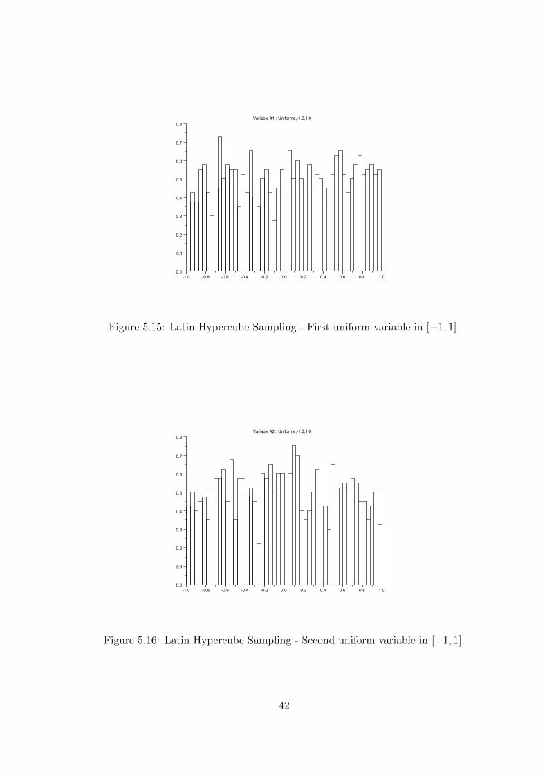
The following Scilab session allows to generate a Monte-Carlo sampling with two uniform variablesin the interval [−1, 1]. The figure 5.14 presents this sampling and the figures 5.15 and 5.16 presentthe histograms of the two uniform random variables.

vu1 = randvar_new("Uniforme" ,-1.0,1.0);

vu2 = randvar_new("Uniforme" ,-1.0,1.0);




setrandvar_buildsample ( srv , "MonteCarlo" , 1000 );


randvar_destroy(vu1);


setrandvar_destroy(srv);

Figure 5.14: Monte-Carlo Sampling - Two uniform variables in the interval [−1, 1].

It is easy to change the type of sampling by modifying the second argument of the setrandvar_buildsamplefunction. This way, we can create the Petras, Quadrature and Sobol sampling presented in figures5.17, 5.18 and 5.19.

41

0.80.60.40.20.0-0.2-0.4-0.6-0.8-1.0

0.8

0.7

0.6

0.5

0.4

0.3

0.2

0.1

0.01.0

Variable #1 : Uniforme,-1.0,1.0

Figure 5.15: Latin Hypercube Sampling - First uniform variable in [−1, 1].

0.80.60.40.20.0-0.2-0.4-0.6-0.8-1.0

0.8

0.7

0.6

0.5

0.4

0.3

0.2

0.1

0.01.0

Variable #2 : Uniforme,-1.0,1.0

Figure 5.16: Latin Hypercube Sampling - Second uniform variable in [−1, 1].

42

Figure 5.17: Petras sampling - Two uniform variables in the interval [−1, 1].

Figure 5.18: Quadrature sampling - Two uniform variables in the interval [−1, 1].

43

Figure 5.19: Sobol sampling - Two uniform variables in the interval [−1, 1].

44

Chapter 6

The polychaos class

6.1 Introduction

The polychaos class allows to manage a polynomial chaos expansion. The coefficients of theexpansion are computed based on given numerical experiments which creates the associationbetween the inputs and the outputs. Once computed, the expansion can be used as a regularfunction. The mean, standard deviation or quantile can also be directly retrieved.

The tool allows to get the following results:

• mean,

• variance,

• quantile,

• correlation, etc...

Moreover, we can generate the C source code which computes the output of the polynomial chaosexpansion. This C source code is stand-alone, that is, it is independent of both the NISP libraryand Scilab. It can be used as a meta-model.

The figure 6.1 presents the most commonly used methods available in the polychaos class.More methods are presented in figure 6.2. The inline help contains the detailed calling sequencefor each function and will not be repeated here. More than 50 methods are available and most ofthem will not be presented here.

More informations about the Oriented Object system used in this toolbox can be found in thesection 4.2.2.

6.2 Examples

In this section, we present to examples of use of the polychaos class.

6.2.1 Product of two random variables

In this section, we present the polynomial expansion of the product of two random variables.We analyse the Scilab script and present the methods which are available to perform the sensi-

45

Constructorspc = polychaos_new ( file )

pc = polychaos_new ( srv , ny )

pc = polychaos_new ( pc , nopt , varopt )

Methodspolychaos_setsizetarget ( pc , np )

polychaos_settarget ( pc , output )

polychaos_setinput ( pc , invalue )

polychaos_setdimoutput ( pc , ny )

polychaos_setdegree ( pc , no )

polychaos_getvariance ( pc )

polychaos_getmean ( pc )

Destructorpolychaos_destroy (pc)

Static methodstokenmatrix = polychaos_tokens ()

nb = polychaos_size ()

Figure 6.1: Outline of the methods of the polychaos class

tivity analysis. This script is based on the NISP methodology, which has been presented in theIntroduction chapter. We will use the figure 1.1 as a framework and will follow the steps in order.

In the following Scilab script, we define the function Example which takes a vector of size 2 asinput and returns a scalar as output.

function y = Exemple (x)

y(:,1) = x(:,1) .* x(:,2)

endfunction

We now create a collection of two stochastic (normalized) random variables. Since the ran-dom variables are normalized, we use the default parameters of the randvar_new function. Thenormalized collection is stored in the variable srvx.

vx1 = randvar_new("Normale");

vx2 = randvar_new("Uniforme");

srvx = setrandvar_new ();

setrandvar_addrandvar ( srvx , vx1 );

setrandvar_addrandvar ( srvx , vx2 );

We create a collection of two uncertain parameters. We explicitely set the parameters of eachrandom variable, that is, the first Normal variable is associated with a mean equal to 1.0 anda standard deviation equal to 0.5, while the second Uniform variable is in the interval [1.0, 2.5].This collection is stored in the variable srvu.

vu1 = randvar_new("Normale" ,1.0 ,0.5);

vu2 = randvar_new("Uniforme" ,1.0 ,2.5);


setrandvar_addrandvar ( srvu , vu1 );

setrandvar_addrandvar ( srvu , vu2 );

46

Methodsoutput = polychaos_gettarget ( pc )

np = polychaos_getsizetarget ( pc )

polychaos_getsample ( pc , k , ovar )

polychaos_getquantile ( pc , k )

polychaos_getsample ( pc )

polychaos_getquantile ( pc , alpha )

polychaos_getoutput ( pc )

polychaos_getmultind ( pc )

polychaos_getlog ( pc )

polychaos_getinvquantile ( pc , threshold )

polychaos_getindextotal ( pc )

polychaos_getindexfirst ( pc )

ny = polychaos_getdimoutput ( pc )

nx = polychaos_getdiminput ( pc )

p = polychaos_getdimexp ( pc )

no = polychaos_getdegree ( pc )

polychaos_getcovariance ( pc )

polychaos_getcorrelation ( pc )

polychaos_getanova ( pc )

polychaos_generatecode ( pc , filename , funname )

polychaos_computeoutput ( pc )

polychaos_computeexp ( pc , srv , method )

polychaos_computeexp ( pc , pc2 , invalue , varopt )

polychaos_buildsample ( pc , type , np , order )

Figure 6.2: More methods from the polychaos class

47

The first design of experiment is build on the stochastic set srvx and based on a Quadraturetype of DOE. Then this DOE is transformed into a DOE for the uncertain collection of parameterssrvu.

degre = 2;

setrandvar_buildsample ( srvx , "Quadrature" , degre );

setrandvar_buildsample ( srvu , srvx );

The next steps will be to create the polynomial and actually perform the DOE. But beforedoing this, we can take a look at the DOE associated with the stochastic and uncertain collectionof random variables. We can use the setrandvar_getsample twice and get the following output.

-->setrandvar_getsample(srvx)

ans =

- 1.7320508 0.1127017

- 1.7320508 0.5

- 1.7320508 0.8872983

0. 0.1127017

0. 0.5

0. 0.8872983

1.7320508 0.1127017

1.7320508 0.5

1.7320508 0.8872983

-->setrandvar_getsample(srvu)

ans =

0.1339746 1.1690525

0.1339746 1.75

0.1339746 2.3309475

1. 1.1690525

1. 1.75

1. 2.3309475

1.8660254 1.1690525

1.8660254 1.75

1.8660254 2.3309475

These two matrices are a 9×2 matrices, where each line represents an experiment and each columnrepresents an input random variable. The stochastic (normalized) srvx DOE has been createdfirst, then the srvu has been deduced from srvx based on random variable transformations.

We now use the polychaos_new function and create a new polynomial pc. The number ofinput variables corresponds to the number of variables in the stochastic collection srvx, that is2, and the number of output variables is given as the input argument ny. In this particular case,the number of experiments to perform is equal to np=9, as returned by the setrandvar_getsize

function. This parameter is passed to the polynomial pc with the polychaos_setsizetarget

function.

ny = 1;

pc = polychaos_new ( srvx , ny );

np = setrandvar_getsize(srvx);

polychaos_setsizetarget(pc,np);

48

In the next step, we perform the simulations prescribed by the DOE. We perform this loop inthe Scilab language and make a loop over the index k, which represents the index of the currentexperiment, while np is the total number of experiments to perform. For each loop, we get theinput from the uncertain collection srvu with the setrandvar_getsample function, pass it tothe Exemple function, get back the output which is then transferred to the polynomial pc by thepolychaos_settarget function.

inputdata = setrandvar_getsample(srvu);

outputdata = Exemple(inputdata );

polychaos_settarget(pc,outputdata );

We can compute the polynomial expansion based on numerical integration so that the coeffi-cients of the polynomial are determined. This is done with the polychaos_computeexp function,which stands for ”compute the expansion”.

polychaos_setdegree(pc,degre);

polychaos_computeexp(pc,srvx ,"Integration");

Everything is now ready for the sensitivity analysis. Indeed, the polychaos_getmean returnsthe mean while the polychaos_getvariance returns the variance.

average = polychaos_getmean(pc);

var = polychaos_getvariance(pc);

mprintf("Mean = %f\n",average );

mprintf("Variance = %f\n",var);

mprintf("Indice de sensibilite du 1er ordre\n");

mprintf(" Variable X1 = %f\n",polychaos_getindexfirst(pc ,1));


mprintf("Indice de sensibilite Totale\n");

mprintf(" Variable X1 = %f\n",polychaos_getindextotal(pc ,1));



Mean = 1.750000

Variance = 1.000000

Indice de sensibilite du 1er ordre

Variable X1 = 0.765625


Indice de sensibilite Totale



In order to free the memory required for the computation, it is necessary to delete all theobjects created so far.

polychaos_destroy(pc);



randvar_destroy(vx1);

randvar_destroy(vx2);

setrandvar_destroy(srvu);

setrandvar_destroy(srvx);

49

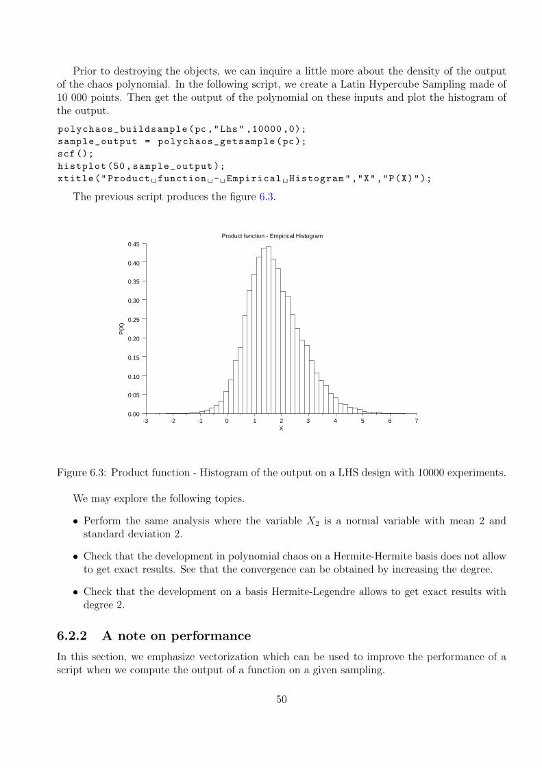
Prior to destroying the objects, we can inquire a little more about the density of the outputof the chaos polynomial. In the following script, we create a Latin Hypercube Sampling made of10 000 points. Then get the output of the polynomial on these inputs and plot the histogram ofthe output.

polychaos_buildsample(pc,"Lhs" ,10000 ,0);

sample_output = polychaos_getsample(pc);

scf();

histplot (50, sample_output );

xtitle("Product function - Empirical Histogram","X","P(X)");


0.00

0.05

0.10

0.15

0.20

0.25

0.30

0.35

0.40

0.45

-3 -2 -1 0 1 2 3 4 5 6 7

Product function - Empirical Histogram

X

P(X

)

Figure 6.3: Product function - Histogram of the output on a LHS design with 10000 experiments.

We may explore the following topics.

• Perform the same analysis where the variable X2 is a normal variable with mean 2 andstandard deviation 2.

• Check that the development in polynomial chaos on a Hermite-Hermite basis does not allowto get exact results. See that the convergence can be obtained by increasing the degree.

• Check that the development on a basis Hermite-Legendre allows to get exact results withdegree 2.

6.2.2 A note on performance

In this section, we emphasize vectorization which can be used to improve the performance of ascript when we compute the output of a function on a given sampling.

50

In order to use vectorization, the core feature that we used in the Exemple is the use of theelementwise multiplication, denoted by .*. In the Exemple function below (reproduced here forsimplicity), the input x is a np-by-2 matrix of doubles, where np is the number of experiments,and y is a np-by-1 matrix of doubles.


y(:,1) = x(:,1) .* x(:,2)

endfunction

The elementwise multiplication allows to multiply the two first columns of x, and sets the resultinto the output y, in one single statement. Since Scilab uses optimized numerical libraries, thisallows to get the best performance in most situations.

In the previous section, we have shown that we can compute the output of the Exemple

function in one single call to the function.


This call allows to produce all the outputs as fast as possible and is the recommended method.The reason is that the previous script lets Scilab perform computations with large matrices.

In fact, there is another, slower, method to perform the same computation. We make a loopover the index k, which represents the index of the current experiment, while np is the totalnumber of experiments to perform. For each loop, we get the input from the uncertain collectionsrvu with the setrandvar_getsample function, pass it to the Exemple function, get back theoutput which is then transferred to the polynomial pc by the polychaos_settarget function.

// This is slow.

for k=1:np

inputdata = setrandvar_getsample(srvu ,k);


mprintf ( "Experiment #%d , input =[%f %f], output = %f\n", k, ..

inputdata (1), inputdata (2) , outputdata )

polychaos_settarget(pc,k,outputdata );

end


Experiment #1, input =[0.133975 1.169052] , output = 0.156623









While the previous script is perfectly correct, it can be very slow when the number of ex-periments is large. This is because the interpreter has to perform a large number of loops withmatrices of small size. In general, this produces much slower script and should be avoided. Moredetails on this topic are presented in [1].

51

6.2.3 The Ishigami test case

In this section, we present the Ishigami test case.The function Exemple is the model that we consider in this numerical experiment. This

function takes a vector of size 3 in input and returns a scalar output.


a=7.

b=0.1

s1=sin(x(:,1))

s2=sin(x(:,2))

y(:,1) = s1 + a.*s2.*s2 + b.*x(: ,3).*x(: ,3).*x(: ,3).*x(: ,3).*s1

endfunction

We create 3 uncertain parameters which are uniform in the interval [−π, π] and put theserandom variables into the collection srvu.

rvu1 = randvar_new("Uniforme",-%pi ,%pi);







The collection of stochastic variables is created with the function setrandvar_new. The callingsequence srvx = setrandvar_new( nx ) allows to create a collection of nx=3 random variablesuniform in the interval [0, 1]. Then we create a Petras DOE for the stochastic collection srvx andtransform it into a DOE for the uncertain parameters srvu.

nx = setrandvar_getdimension ( srvu );

srvx = setrandvar_new( nx );

degre = 9;

setrandvar_buildsample(srvx ,"Petras",degre );

setrandvar_buildsample( srvu , srvx );

We use the polychaos_new function and create the new polynomial pc with 3 inputs and 1output.

noutput = 1;

pc = polychaos_new ( srvx , noutput );

The next step allows to perform the simulations associated with the DOE prescribed by thecollection srvu. Here, we must perform np=751 experiments.

np = setrandvar_getsize(srvu);

polychaos_setsizetarget(pc,np);

inputdata = setrandvar_getsample(srvu);


polychaos_settarget(pc ,outputdata );

We can now compute the polynomial expansion by integration.

polychaos_setdegree(pc ,degre );

polychaos_computeexp(pc,srvx ,"Integration");

52

Everything is now ready so that we can do the sensitivy analysis, as in the following script.

average = polychaos_getmean(pc);

var = polychaos_getvariance(pc);

mprintf("Mean = %f\n",average );

mprintf("Variance = %f\n",var);

mprintf("First order sensitivity index\n");




mprintf("Total sensitivity index\n");





Mean = 3.500000

Variance = 13.842473

First order sensitivity index




Total sensitivity index




We now focus on the variance generated by the variables #1 and #3. We set the groupto the empty group with the polychaos_setgroupempty function and add variables with thepolychaos_setgroupaddvar function.

groupe = [1 3];

polychaos_setgroupempty ( pc );

polychaos_setgroupaddvar ( pc , groupe (1) );

polychaos_setgroupaddvar ( pc , groupe (2) );

mprintf("Fraction of the variance of a group of variables\n");

mprintf(" Groupe X1 et X2 =%f\n",polychaos_getgroupind(pc));


Fraction of the variance of a group of variables

Groupe X1 et X2 =0.557674

The function polychaos_getanova prints the functionnal decomposition of the normalizedvariance.

polychaos_getanova(pc);


1 0 0 : 0.313953

0 1 0 : 0.442325

1 1 0 : 1.55229e-009

0 0 1 : 8.08643e-031

53

1 0 1 : 0.243721

0 1 1 : 7.26213e-031

1 1 1 : 1.6007e-007

We can compute the density function associated with the output variable of the function. Inorder to compute it, we use the polychaos_buildsample function and create a Latin HypercubeSampling with 10000 experiments. The polychaos_getsample function allows to quiery thepolynomial and get the outputs. We plot it with the histplot Scilab graphic function, whichproduces the figure 6.4.

polychaos_buildsample(pc,"Lhs" ,10000 ,0);

sample_output = polychaos_getsample(pc);

scf();

histplot (50, sample_output)

xtitle("Ishigami - Histogram");

151050-5-10

0.12

0.10

0.08

0.06

0.04

0.02

0.0020

Fonction Ishigami - Histogramme normalisé

Figure 6.4: Ishigami function - Histogram of the output of the chaos polynomial on a LHS designwith 10 000 experiments.

We can plot a bar graph of the sensitivity indices, as presented in figure 6.5.

for i=1:nx

indexfirst(i)= polychaos_getindexfirst(pc,i);

indextotal(i)= polychaos_getindextotal(pc,i);

end

scf();

54

bar(indextotal ,0.2,’blue ’);

bar(indexfirst ,0.15,’yellow ’);

legend (["Total" "First order"],pos =1);

xtitle("Ishigami - Sensitivity indices");

Figure 6.5: Ishigami function - Sensitivity indices.

55

Chapter 7

Thanks

Many thanks to Allan Cornet.

56

Bibliography

[1] Michael Baudin. Programming in scilab, 2010.

[2] Michael Baudin and Jean-Marc Martinez. Polynomes de chaos sous scilab via la librairie nisp.In 42emes Journees de Statistique, 24 au 28 mai 2010 - Marseille, France, 2010.

[3] Didier Pelat. Bases et methodes pour le traitement des donnees (Bruits et Signaux). MasterM2 Recherche : Astronomie?astrophysique, 2006.

57

Documents

NISP Toolbox Manual - Scilabforge.scilab.org/upload/nisp/files/nisp_toolbox_manual... · 2012-02-08 · "Open-Source Platform for Uncertainty treatments in Simulation", funded by