NIH Public Access Zhaohua Lu Joseph G. Ibrahim Alzheimer's ... · Neuroimaging Phenotypes and Genetic Markers Hongtu Zhu , Zakaria Khondker , Zhaohua Lu , Joseph G. Ibrahim , and

Bayesian Generalized Low Rank Regression Models for Neuroimaging Phenotypes and Genetic Markers

Hongtu Zhu, Zakaria Khondker, Zhaohua Lu, Joseph G. Ibrahim, and Alzheimer's Disease Neuroimaging Initiative‡

H. Zhu is Professor of Biostatistics ([email protected]), Z. Khondker was a Ph.d student under the supervision of Drs. Ibrahim and Zhu ([email protected]), Z. Lu was a postdoctoral fellow under the supervision of Dr. Zhu ([email protected]), and J. G. Ibrahim is Alumni Distinguished Professor of Biostatistics ([email protected]), Department of Biostatistics, University of North Carolina at Chapel Hill, NC 27599-7420

Abstract

We propose a Bayesian generalized low rank regression model (GLRR) for the analysis of both

high-dimensional responses and covariates. This development is motivated by performing

searches for associations between genetic variants and brain imaging phenotypes. GLRR

integrates a low rank matrix to approximate the high-dimensional regression coefficient matrix of

GLRR and a dynamic factor model to model the high-dimensional covariance matrix of brain

imaging phenotypes. Local hypothesis testing is developed to identify significant covariates on

high-dimensional responses. Posterior computation proceeds via an efficient Markov chain Monte

Carlo algorithm. A simulation study is performed to evaluate the finite sample performance of

GLRR and its comparison with several competing approaches. We apply GLRR to investigate the

impact of 1,071 SNPs on top 40 genes reported by AlzGene database on the volumes of 93 regions

of interest (ROI) obtained from Alzheimer's Disease Neuroimaging Initiative (ADNI).

Keywords

Generalized low rank regression; Genetic variant; High dimension; Imaging phenotype; Markov chain Monte Carlo; Penalized method

1 Introduction

The emergence of high-dimensional data in genomics and neuroimaging, among other areas,

has presented us with a large number of predictors as well as many response variables,

which may have strong correlations. For instance, in imaging genetics as an emerging field,

such problems frequently arise when multivariate imaging measures, such as volumes of

cortical and subcortical regions of interest (ROIs), are predicted by high-dimensional

covariate vectors, such as gene expressions or single nucleotide polymorphisms (SNPs). The

joint analysis of imaging and genetic data may ultimately lead to discoveries of genes for

some complex mental and neurological disorders, such as autism and schizophrenia (Cannon

‡Address for correspondence and reprints: Hongtu Zhu, Ph.D., [email protected]; Phone No: 919-966-7272..

NIH Public AccessAuthor ManuscriptJ Am Stat Assoc. Author manuscript; available in PMC 2015 January 01.

Published in final edited form as:J Am Stat Assoc. 2014 ; 109(507): 997–990.

NIH

-PA

Author M

anuscriptN

IH-P

A A

uthor Manuscript

NIH

-PA

Author M

anuscript

and Keller, 2006; Turner et al., 2006; Scharinger et al., 2010; Paus, 2010; Peper et al., 2007;

Chiang et al., 2011a,b). This motivates us to develop low rank regression models (GLRR)

for the analysis of high-dimensional responses and covariates under the high-dimension-

low-sample-size setting.

Developing models for high-dimensional responses and covariates poses at least four major

challenges including (i) a large number of regression parameters, (ii) a large covariance

matrix, (iii) correlations among responses, and (iv) multicollinearity among predictors.

When the number of responses and the number of covariates, which are denoted by d and p,

respectively, are even moderately high, fitting conventional multivariate response regression

models (MRRM) usually requires estimating a d × p matrix of regression coefficients,

whose number pd can be much larger than the sample size. Although accounting for

complicated correlation among multiple responses is important for improving the overall

prediction accuracy of multivariate analysis (Breiman and Friedman, 1997), it requires

estimating d(d + 1)/2 unknown parameters in a d × d unstructured covariance matrix.

Another notorious difficulty is that the collinearity among a large number of predictors can

cause issues of over-fitting and model misidentification (Fan and Lv, 2010).

There is a great interest in developing new statistical methods to handle these challenges for

MRRMs. The early developments involve a separation approach–variable selection to

reduce dimension and then parameter estimation, when both p and d are moderate compared

to the sample size (Breiman and Friedman, 1997). For instance, Brown et al. (2002)

introduced Bayesian model averaging incorporating variable selection for prediction, which

allows for fast computation for dimensions up to several hundred. Recently, much attention

has been given to shrinkage methods for achieving better stability and improving

performance (Tibshirani, 1996). Notably, the most popular ones are the L1 and L2 penalties.

The L2 penalty forces the coefficients of highly correlated covariates towards each other,

whereas the L1 penalty usually selects only one predictor from a highly correlated group

while ignoring the others. L1 priors can be seen as sparse priors since they create a

singularity at the origin whose gravity pulls the smaller coefficients to zero under maximum

a posteriori (MAP) estimation. There are fully Bayesian approaches with sparse priors for

univariate responses like the Bayesian LASSO (Park and Casella, 2008), a generalization of

the LASSO (Kyung et al., 2010), and the double Pareto (Armagan et al., 2011), among many

others. These methods, however, are primarily developed under the univariate-response-

high-dimensional-covariate setting.

There have been several attempts in developing new methods under the high-dimensional-

response-and-covariate setting. When both p and d are moderate compared to the sample

size, Breiman and Friedman (1997) introduced a Curds and Whey (C&W) method to

improve prediction error by accounting for correlations among the response variables. Peng

et al. (2010) proposed a variant of the elastic net to enforce sparsity in the high-dimensional

regression coefficient matrix, but they did not account for correlations among responses.

Rothman et al. (2010) proposed a simultaneous estimation of a sparse coefficient matrix and

sparse covariance matrix to improve on estimation error under the L1 penalty. Similarly, Yin

and Li (2011) presented a sparse conditional Gaussian graphical model in order to study the

conditional independent relationships among a set of gene expressions adjusting for possible

Zhu et al. Page 2

J Am Stat Assoc. Author manuscript; available in PMC 2015 January 01.

NIH

-PA

Author M

anuscriptN

IH-P

A A

uthor Manuscript

NIH

-PA

Author M

anuscript

genetic effects. Furthermore, several authors have explored the low rank decomposition of

the regression coefficient matrix and then use sparsity-inducing regularization techniques to

reduce the number of parameters (Izenman, 1975; Reinsel and Velu, 1998; Tibshirani, 1996;

Turlach et al., 2005; Chen et al., 2012; Vounou et al., 2010). For instance, Chen et al. (2012)

and Vounou et al. (2010) considered the singular value decomposition of the coefficient

matrix and used the LASSO-type penalty on both the left and right singular vectors to ensure

its sparse structure. Since all variable selection methods require a selection of a proper

amount of regularization for consistent variable selection, some methods, such as stability

selection and cross validation, are needed for such selection (Meinshausen and Buhlmann,

2010). They, however, do not provide a standard inference tool (e.g., standard deviation) on

the nonzero components of the left and right singular vectors or the coefficient matrix.

Moreover, frequentist inference is the primary approach for making statistical inferences in

the high-dimensional-response-and-covariate setting.

In this paper, we propose a new Bayesian GLRR to model the association between genetic

variants and brain imaging phenotypes. A low rank regression model is introduced to

characterize associations between genetic variants and brain imaging phenotypes, while

accounting for the impact of other covariates. We assume shrinkage priors on the singular

values of the regression coefficient matrix, while not explicitly requiring orthonormality of

left and right singular vectors. This facilitates fast computation of the regression coefficient

matrix. We consider a sparse latent factor model to more flexibly capture the within-subject

correlation structure and assume a multiplicative gamma process shrinkage priors on the

factor loadings, which allow for the introduction of infinitely many factors (Bhattacharya

and Dunson, 2011). We propose Bayesian local hypothesis testing to identify significant

effects of genetic markers on imaging phenotypes, while controlling for multiple

comparisons. Posterior computation proceeds via an efficient Markov chain Monte Carlo

(MCMC) algorithm.

In Section 2, we introduce the NIH Alzheimer's Disease Neuroimaging Initiative (ADNI)

dataset. In Section 3, we introduce GLRR and its associated Bayesian estimation procedure.

In Section 4, we conduct simulation studies with a known ground truth to examine the finite

sample performance of GLRR and compare it with the conventional LASSO method.

Section 5 illustrates an application of GLRR in the joint analysis of imaging, genetic, and

clinical data from ADNI. Section 6 presents concluding remarks.

2 Generalized Low Rank Regression Models

2.1 Model Setup

Consider imaging genetic data from n independent subjects in ADNI. For each subject, we

observe a d × 1 vector of imaging measures, denoted by Yi = (yi1, …, yid)T, and a p × 1

vector of clinical and genetic predictors, denoted by Xi = (xi1, …, xip)T, for i = 1, …, n. Let Y = (yik) be an n × d matrix of mean centered responses, X = (xij) be an n × p matrix of

standardized predictors, B = (βjk) be a p × d matrix of regression coefficients, and E = (∊ik)

be an n × d matrix of residuals. We consider a multivariate response regression model given

by

Zhu et al. Page 3


NIH

-PA

Author M

anuscriptN

IH-P

A A

uthor Manuscript

NIH

-PA

Author M

anuscript

(1)

where ∊i ~ Nd(0, Σ = Θ−1), in which Θ = Σ−1 is the d × d precision matrix. There are several

statistical challenges in fitting model (1) to real data. When both p and d are relatively large

compared to n, the number of parameters in B equals p × d and can be much larger than n.

Furthermore, the number of unknown parameters in Σ equals d(d+1)/2. In addition to the

number of unknown parameters, there are some additional complexities arising from

practical applications, including different scales for different response variables and

collinearity among the predictors.

In model (1), multiple responses are measured from the same subject and share a set of

common predictors. Therefore, the regression coefficient matrix B can have two-way linear

dependence coming from both the correlated responses and covariates. This shared mean

structure can lead to a low rank mean parameter matrix B. We exploit this shared structure

of B by decomposing it as

(2)

where r is the rank of B, Bl = δlulvlT is the l−th layer for l = 1, …, r, Δ = diag(δ1, …, δr), U =

[u1, …, ur] is a p × r matrix, and V = [v1, …, vr] is a d × r matrix. In (2), it is assumed that

genetic variates that are associated with phenotypes may be relatively sparse and each

column of U may group informative SNPs with similar association into clusters. Thus, under

such assumption, a small rank of B may capture the major dependence structure between Yi

and Xi.

Given the large number of parameters in Σ, we consider a Bayesian factor model to relate

the random effects ∊i to the latent factors ηi as

(3)

where Λ is a d × ∞ factor loading matrix, ηi ~ N∞(0, I∞), and ξi ~ N(0, Σξ) with

. As shown in Hyun et al. (2014), the factor model (3) is useful for

delineating the medium-to-long-range (or global) spatial dependence of neuroimaging data.

Another advantage of (3) is that it bypasses the challenging issue of selecting the number of

factors through a delicate prior setting. To achieve dimensionality reduction, one would

typically restrict the dimension of the latent factor vector ηi to be orders of magnitude less

than that of ∊i. By following Bhattacharya and Dunson (2011), we choose a prior that

shrinks the elements of to zero as the column index increases. Thus, it bypasses the

challenging issue of selecting the number of factors. Finally, our GLRR integrates the low

rank model (2) and the Bayesian factor model (3). Specifically, our GLRR can be written as

(4)

Zhu et al. Page 4


NIH

-PA

Author M

anuscriptN

IH-P

A A

uthor Manuscript

NIH

-PA

Author M

anuscript

Other than genetic markers, such as SNP's, it is common that Xi has a subvector, denoted by

XPi, consisting of several prognostic variables, such as age, gender, and disease status in real

applications. There are two different methods to deal with prognostic factors in the presence

of genetic markers. The first method is a two-step approach. The first step is to fit the

MRRM solely with these prognostics factors as covariates and then calculate the fitted

residuals as adjusted responses. The final step is to fit model (4) to the adjusted responses

with genetic markers as X. The second method is to fit model (4) with both prognostic

factors and genetic markers as covariates. Let BP be the pP × d matrix of coefficients

associated with the prognostic factors and XSi and BS be, respectively, the subvector of Xi

and the submatrix of B associated with genetic markers. It may be reasonable to assume that

BP may be unstructured and BS admits the decomposition given by

. In this case, the model can be written as

(5)

We take the second approach and fit model (5) in real data analysis.

2.2 Low Rank Approximation

The decomposition (2) is similar to the standard singular value decomposition (SVD), but it

differs from SVD. Specifically, it is unnecessary that the columns of U and V in (2) are

orthonormal and this allows that ujl and vjl can take any value in (−∞, ∞), since

identifiability is not critical for making inference on B. Thus, the decomposition (2) can be

regarded as a generalization of SVD in Chen et al. (2012). Moreover, compared to SVD, this

decomposition leads to better computational efficiency, since sampling a unit vector in a

high-dimensional sphere is computationally difficult. Nevertheless, each layer Bl is a

factorization with unit rank, which amounts to estimating a common p × 1 vector of distinct

regression coefficients and making the rest of the coefficients some linear combinations of

this vector with d additional parameters. Within the l-th layer, each column of Bl shares the

same ul and δl, which facilitates the exploitation of a common dependence structure among

the covariates collected from the same set of subjects. Similarly, each row of Bl shares the

same vl and δl facilitating the exploitation of a common dependence structure among the

responses from the same set of subjects. The number of parameters at each layer is p + d and

the total number of parameters equals r × (p + d). Since r << min(p, d), the use of the

decomposition (2) leads to a huge dimension reduction.

The decomposition (2) differs from two other popular methods including multivariate

response models and stepwise unit rank regression models. Multivariate response models

estimate a separate p×1 vector of coefficients for each response totaling p×d parameters. In

frequentist analysis (Chen et al., 2012), it is common to sequentially explore each layer of B

based on the ordering of Δ, which leads to stepwise unit rank regressions (SURR).

Specifically, one first fits the unit rank (r = 1) regression with the observed Y as the response

to estimate the first layer and . Subsequently, one fits another unit rank

Zhu et al. Page 5


NIH

-PA

Author M

anuscriptN

IH-P

A A

uthor Manuscript

NIH

-PA

Author M

anuscript

regression with as the response to estimate the second layer . One can continue

this process until the r-th rank. Thus, SURR can be viewed as a special case of GLRR.

2.3 Covariance Structure

The covariance structure for Yi is given by

(6)

It is common to impose a constraint on Λ to define a unique model free from identification

problems, since Σ is invariant under the transformation Λ* = ΛP for any semi-orthogonal

matrix P with P PT = I. For instance, for identifiability purposes, one may impose a full rank

lower triangular constraint, which implicitly specifies an order dependence among the

responses (Geweke and Zhou, 1996). However, it is unnecessary to impose such a constraint

on Λ if our primary interest is on covariance matrix estimation. Specifically, we will specify

a multiplicative gamma process shrinkage prior in (7) on a parameter expanded loading

matrix with redundant parameters. The induced prior on Σ is invariant to the ordering of the

responses. This shrinkage prior adaptively selects a truncation of the infinite loadings to one

having finite columns. Thus, it facilitates the posterior computation and provides an accurate

approximation to the infinite factor model.

2.4 Priors

We first consider the priors on the elements of all layers Bl. When dealing with two highly

correlated covariates, the L1 prior tends to pick one and drop the other since it is typically a

least angle selection approach to force some coefficients to zero, whereas the L2 prior tends

to force the coefficients towards each other to produce two highly correlated coefficients. In

GLRR, since our primary interest is to exploit the potential two-way correlations among the

estimated coefficients, we choose the L2 prior. Let Ga(a, b) be a gamma distribution with

scale a and shape b. Specifically, we choose

where a0, b0, c0, d0, e0, and f0 are prefixed hyper-parameters. The number of predictors p is

included in the hyperprior of τu to have a positive-definite covariance matrix of high

dimensional ul and fix the scale of ul. Similarly, we add the dimension d to all hyper-priors

for τv,l. Moreover, we standardize all predictors to have zero mean and unit variance, and

thus a single prior is sensible for all elements of ul. The varying dispersions τv,1, …, τv,d are

chosen to account for different scales of different responses. For example, the volumes of

Zhu et al. Page 6


NIH

-PA

Author M

anuscriptN

IH-P

A A

uthor Manuscript

NIH

-PA

Author M

anuscript

different ROIs vary dramatically across ROIs, so it is more sensible to use separate

dispersions for different ROIs.

We place the multiplicative gamma process shrinkage prior (Bhattacharya and Dunson,

2011) on Λ in order to increasingly shrink the factor loadings towards zero with the column

index. Such shrinkage priors avoid the drawback of order dependence from the lower

triangular constraint on Λ for identifiability. We use inverse gamma priors on the diagonal

elements of Σξ. Specifically, these priors are given as follows:

(7)

where ψg for g = 1, …, ∞ are independent random variables, τλh is a global shrinkage

parameter for the h-th column, and the ϕkhs are local shrinkage parameters for the elements

in the h-th column. Moreover, v, a1,, a2, aσk and bσk are prefixed hyper-parameters. When a2

> 1, the τλh's increase stochastically with the column index h, which indicates more

shrinkage favored over the columns of higher indices. The loading component specific prior

precision allows shrinking the components of Λ. Straightforward Gibbs sampler can

be applied for posterior computation

2.5 Posterior Computation

We propose a straightforward Gibbs sampler for posterior computation after truncating the

loadings matrix to have k* << d columns. An adaptive strategy for inference on the

truncation level k* has been described in (Bhattacharya and Dunson, 2011). The Gibbs

sampler is computationally efficient and mixes rapidly. Starting from the initiation step, the

Gibbs sampler at the truncated level k* proceeds as follows:

1. Update (ul, τu) according to their conditional distributions

where .

2. Update (vl, τv,k) according to their conditional distributions

for k = 1, …, d, where .

3. Update (δl, τδ) according to their conditional distributions

Zhu et al. Page 7


NIH

-PA

Author M

anuscriptN

IH-P

A A

uthor Manuscript

NIH

-PA

Author M

anuscript

where .

4. Update the kth row of Λk*, denoted by τk, from its conditional distribution

where η = (η1, …, ηn)T, Ek = (∊1k, …, ∊nk)T is the kth column of E = Y − XB, and

for k = 1, …, d.

5. Update ϕkh from its conditional distribution

6. Update ψ1 from its conditional distribution

and update ψh, h ≥ 2 from its conditional distribution

where for h = 1, …, k*.

7. Update , k = 1, …, d, from its conditional distribution

8. Update ηi, i = 1, …, n, from conditionally independent posteriors

where ∊i is the ith row of E.

Zhu et al. Page 8


NIH

-PA

Author M

anuscriptN

IH-P

A A

uthor Manuscript

NIH

-PA

Author M

anuscript

2.6 Determining the Rank of B

We consider different methods for determining the rank of B. For frequentist inference,

many regularization methods have been developed to recover the low rank structure of a

matrix, such as B, by shrinking δℓ's to zero in (2) (Chen et al., 2012). For Bayesian

inference, it may be tempting to use Bayesian model averaging and allow varying number of

layers in order to improve prediction performance, but it limits us on making statistical

inference on each layer of B, U, and V . We take a fixed-rank approach and use some

selection criteria to choose an optimal value of r. Specifically, we consider five different

selection criteria including the Akaike information criterion (AIC), the Bayesian information

criterion (BIC), the normalized prediction error (PEN), the multivariate R2, and the

normalized model error (MEN) for GLRR. Let , where is the posterior estimate of

B based on the MCMC samples. Let be the error sum of

squares and p* = r(p + d) be the number of parameters in B. The five evaluation criteria are,

respectively, given by

(8)

The numerator and denominator of the MEN are, respectively, the model error and

measurement error of model (4) (Yuan et al., 2007). Thus, the MEN is the ratio of the model

error over the measurement error as a percentage of the total magnitude of all parameters.

Similarly, the PEN and R2 are defined as percentages, which makes comparisons more

meaningful and readily comparable across studies.

To illustrate the effectiveness of all five criteria, we independently simulated 100 data sets

from model (4) with (n, p, d) = (100, 200, 100) and a rank 5 matrix B. For each simulated

data set, we used the Gibbs sampler to draw posterior samples to estimate B and then

calculated the five selection criteria in (8) as the rank varied from 1 to 10. Finally, based on

all 100 simulated data sets, we calculated the mean and standard deviation of each selection

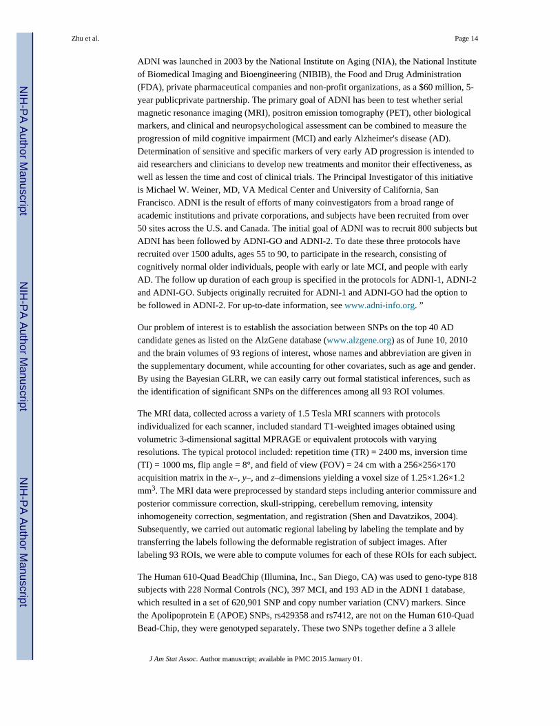
criterion as the rank varied from 1 to 10. As shown in Figure 1, PEN, MEN, R2, and AIC

stabilize around the true rank, whereas BIC reaches the minimum at the true rank. This may

indicate that BIC outperforms other selection criteria for determining the true rank of B. This

result also agrees with the findings in Bozdogan (1987) such that in parametric settings, AIC

tended to select a larger model than the true model even for large sample sizes, whereas BIC

is asymptotically consistent in estimating the true model.

2.7 Thresholding

Based on the MCMC samples obtained from the Gibbs sampler, we are able to identify three

different sets of information including (i) SNPs that significantly contribute to a large

portion of imaging phenotypes, (ii) imaging phenotypes that are associated with those SNPs

in (i), and (iii) important individual SNP effects on individual imaging phenotypes.

Zhu et al. Page 9


NIH

-PA

Author M

anuscriptN

IH-P

A A

uthor Manuscript

NIH

-PA

Author M

anuscript

Statistically, (i), (ii), and (iii) can be formulated as testing significant elements in U, V , and

B, respectively. For the sake of space, we focus on (i). Suppose that we draw a set of

MCMC samples for m = 1, …, M. Due to the magnitude ambiguity of U, we

normalize each column of U = (ujl) to calculate . Moreover, we develop a specific

strategy to deal with the sign ambiguity of U*. For the l–th column of U*, we use the

normalized MCMC samples to empirically determine the j0–th row such

that for all j′ ≠ j0. Then, we fix to be

positive for l = 1, …, r and m = 1, …, M.

To detect SNPs in (i), we suggest to calculate the median and median absolute deviation

(MAD) of , denoted by and su,jl, respectively, since the MCMC samples

may oscillate dramatically between the positive solution and the negative solution due to the

sign ambiguity for all j, l. Then, one may formulate it as testing the local null and alternative

hypotheses for relative to su,jl given by

where T* is a specific threshold for each . One may calculate the probability of

given the observed data and then adjust for multiple

comparisons (Müller et al., 2004; Wang and Dunson, 2010). Another approach is to directly

calculate tu,jl and apply standard multiple comparison methods, such as the false discovery

rate, to determine T* (Benjamini and Hochberg, 1995). We have found that these two

methods lead to similar results, and thus we take the second approach. Moreover, this

Bayesian thresholding method works well even when different responses are not on the

same scale. Compared to the `hard' thresholding methods used in shrinkage methods (Chen

et al., 2012; Peng et al., 2010; Rothman et al., 2010; Yin and Li, 2011), this Bayesian

thresholding method accounts for the variation of each and has a probabilistic

interpretation.

3 Simulation Study

3.1 Simulation Setup

We carried out some simulation studies to examine the finite-sample performance of the

GLRR and its posterior computation. We generated all simulated data according to model

(4). The simulation studies were designed to establish the association between a relatively

high-dimensional phenotype vector with a set of continuous covariates or a set of commonly

used genetic markers (e.g., SNP). For each case, 100 simulated data sets were generated.

We simulated ∊i ~ Nd(0, Σ) and used two types of covariates including (i) continuous

covariates generated from Xi ~ Np(0, ΣX) and (ii) actual SNPs from ADNI data set. We

determined Σ and ΣX as follows. Let p0 be the binomial probability, which controls the

sparsity of the precision matrix. We first generated a p×p matrix A = (ajj′) with ajj = 1 and

Zhu et al. Page 10


NIH

-PA

Author M

anuscriptN

IH-P

A A

uthor Manuscript

NIH

-PA

Author M

anuscript

ajj′ = uniform(0, 1) × binomial(1, p0) for j ≠ j′, set ΣX = AAT, and standardized ΣX into a

correlation matrix such that ΣX,jj = 1 for j = 1, …, d. Similarly, we used the same method to

generate Σ, the covariance matrix of ∊i. For both Σ and ΣX, we set about 20% of the

elements of Σ−1 and to be zero, yielding that the means of the absolute correlations of Σ

and ΣX are close to 0.40, respectively. We chose actual SNPs from the ADNI data set.

Specifically, we only considered the 10,479 SNPs collected on chromosome 19, screened

out all SNPs with more than 5% missing data and minor allele frequency (MAF)< 0.05, and

randomly selected 400 SNPs from the remaining SNPs. For n = 1, 000 case, 500 subjects

were randomly chosen and then replicated twice, whereas for the n=100 case, 100 subjects

were randomly chosen from ADNI data set.

We considered five structures of B in order to examine the finite-sample performance of

GLRR under different scenarios.

• Case 1: Xi ~ Np(0, ΣX) and a “+” structure was preset for B with (p, d) = (100, 100)

with the elements of B being set as either 0 or 1.

• Case 2: Xi × Np(0, ΣX) and B was set as a 200 × 100 matrix with the true rank r0 =

5. Specifically, we set B = UΔV with U = (ujl), Δ = diag(δll) = diag(100, 80, 60, 40,

20), and V = (vlk) being 200 × 5, 5 × 5, and 5 × 100 matrices, respectively.

Moreover, we generated all elements ujl and vlk independently from a N(0, 1)

generator and then orthonormalized U and V.

• Case 3: Covariates are actual SNPs and B has the same structure as that in Case 2

but with (p, d) = (400, 100).

• Case 4: Xi ~ Np(0, ΣX) and B was set as a 200 × 100 matrix with high degrees of

correlation among elements with an average absolute correlation of 0.8, and then

20% of the elements of B were randomly forced to 0. After enforcing zeros, the true

rank is 100 and the average absolute correlation is close to 0.7.

• Case 5: Covariates are actual SNPs and B is the same as that in Case 4 with (p, d) =

(400, 100).

We chose noninformative priors for the hyperparameters of B and set α0 = β0 = a0 = b0 = c0

= d0 = e0 = f0 = 10−6. Since shrinkage is achieved through dimension reduction by choosing

r << min(d, p), these noninformative choices of the hyperparameters suit well. For the

hyperparameters of Σ, we chose somewhat informative priors in order to impose the

positive-definiteness constraint and set ν = a1 = b2 = aσk = bσk = 1 for k = 1, …, d. The

induced prior of Σ ensure that Σ is positive definite, while the prior variances are large

enough to allow Σ to be primarily learned from the data. For each simulated dataset, we ran

the Gibbs sampler for 10,000 iterations with 5, 000 burn-in iterations.

As a comparison, we considered a multivariate version of LASSO (Peng et al., 2010),

Bayesian LASSO (BLASSO) (Park and Casella, 2008), and group-sparse multitask

regression and feature selection (G-SMuRFS) (Wang et al., 2012) for all simulated data. For

LASSO, we fitted d separate LASSO regressions to each response with a single tuning

parameter across all responses by using a 5-fold cross validation. Since variances of all

columns X and E are relatively equal, the variances of all columns of Y should be close to

Zhu et al. Page 11


NIH

-PA

Author M

anuscriptN

IH-P

A A

uthor Manuscript

NIH

-PA

Author M

anuscript

each other. In this case, a single tuning parameter is sensible. For BLASSO, we chose single

priors for each column of the response matrix by setting all hyperparameters to unity. For G-

SMuRFS, we used single group and selected the optimal values of the penalty parameters by

using a 5-fold cross validation.

To compare different methods, we calculated their sensitivity and specificity scores under

each scenario. For all regularization methods, since we choose all possible values of the

tuning parameters for calculating their sensitivity and specificity scores, it is unnecessary to

use the cross validation method to select the tuning parameters. Let I(·) be an indicator

function of an event and , where and sβ,jk denote the posterior mean and

standard deviation of βjk, respectively. Specifically, for a given threshold T0, sensitivity and

specificity scores are, respectively, given by

where TP(T0), TP(T0), TP(T0), and TP(T0) are, respectively, the numbers of true positives,

false positives, true negatives, and false negatives, given by

Varying T0 gives different sensitivity and specificity scores, which allow us to create

receiver operating characteristic (ROC) curves. In each ROC curve, sensitivity is plotted

against 1-specificity. The larger the area under the ROC curve, the better a method in

identifying the true positives while controlling for the false positives.

3.2 Results

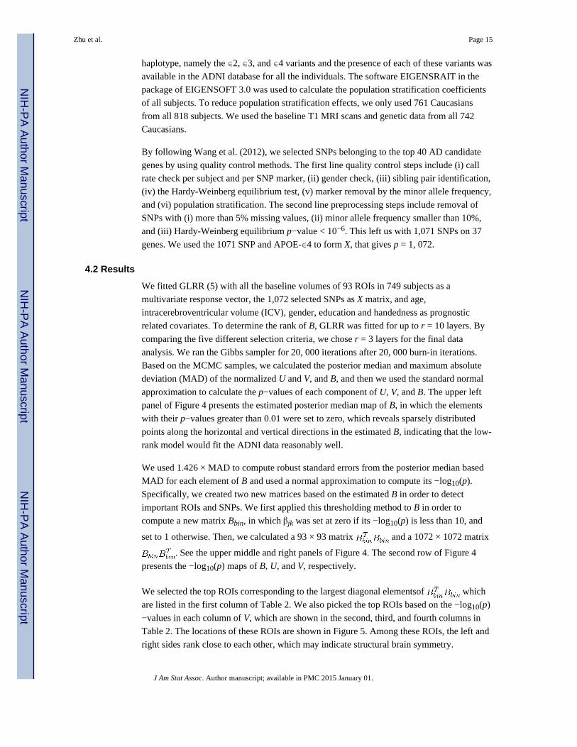
We first performed a preliminary analysis by using five data sets simulated according to the

five structures of B and n = 1, 000. See Figure 2 for the true B and estimated by using

GLRR3 (GLRR with r = 3), GLRR5 (GLRR with r = 5), BLASSO, G-SMuRFS, and

LASSO under Case 1-Case 5. Inspecting Figure 2 reveals that for relatively large sample

sizes, the fitted GLRR with r close to the true rank does a better job in recovering the

underlying structure of B, while BLASSO and G-SMuRFS perform reasonably well for all

cases. For the ”+” structure of B with the true rank r0 = 2 in Case 1, GLRR3 performs the

best, whereas LASSO does a poor job. For B with the true rank r0 = 5 in Cases 2 and 3,

GLRR5 performs the best. The LASSO method performs reasonably well in recovering B

for continuous X, when B is a 200 × 100 matrix, whereas it performs poorly when X is the

SNP matrix. For the high-rank B in Cases 4 and 5, LASSO performs the best in recovering

B, while GLRR3 and GLRR5 perform reasonably well.

Zhu et al. Page 12


NIH

-PA

Author M

anuscriptN

IH-P

A A

uthor Manuscript

NIH

-PA

Author M

anuscript

Secondly, we examined the finite sample performance of LASSO, BLASSO, G-SMuRFS,

GLRR3, and GLRR5 under Cases 1-5 for n = 100. In each case, 100 simulated data sets

were used and the mean and standard deviation of each of the five selection criteria were

calculated. The results are presented in Table 1. Inspecting Table 1 reveals that GLRRs

outperform LASSO in most cases. As p increases, GLRRs outperform LASSO in terms of

MEN, PEN, and R2. Under Cases 3 and 5, GLRRs outperform LASSO with much smaller

errors as well as lower standard deviations for MEN and PEN. LASSO performs much

better for continuous covariates than for discrete SNPs, but such patterns do not appear for

GLRRs. The results of GLRRs and BLASSO are comparable in terms of both AIC and BIC,

but the number of parameters under GLRRs is much smaller than that under BLASSO.

BLASSO and G-SMuRFS perform well in terms of both model error and prediction. The

high R2 and low prediction error of BLASSO and G-SMuRFS in the high dimension cases

may be caused by over-fitting and model misidentification (Fan and Lv, 2010).

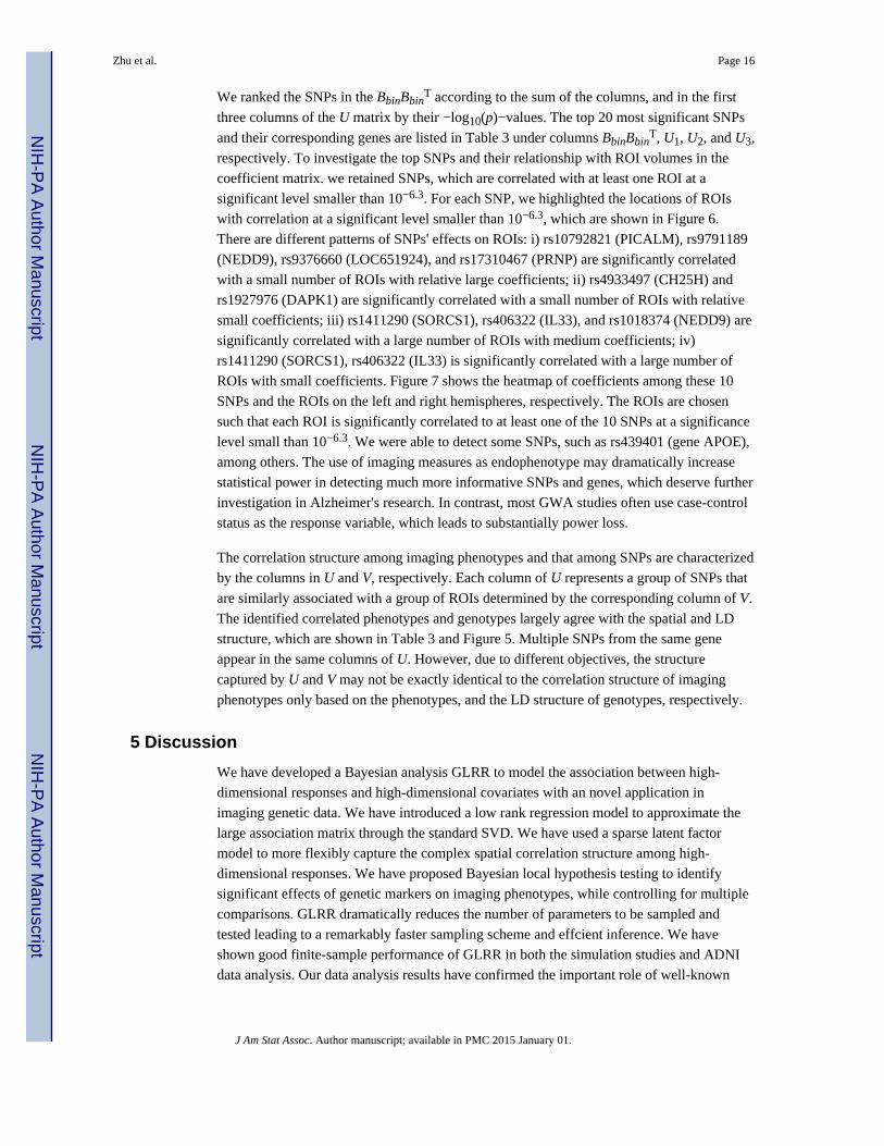
Thirdly, we used the ROC curve to compare LASSO, BLASSO, G-SMuRFS, GLRR3, and

GLRR5 under Cases 1-5. See Figure 3 for details. For Case 1, BLASSO demonstrates

consistently the best power for almost every level of specificity, while G-SMuRFS is the

second best. GLRR3 and GLRR5 fall in the middle. For Case 4, all the methods appear to be

comparable with GLRR3 and GLRR5. For Cases 2, 3, and 5, GLRRs consistently

outperform all other methods.

We also compared the timing of each method in a personal laptop with Intel Core i5 1.7

GHz processor and 4 GB memory. It takes LASSO and G-SMuRFS roughly 5 minutes to

choose the optimal penalty and calculate estimates for a single sample of Case 5. All

Bayesian methods take much longer since one has to sample many MCMC samples.

Specifically, BLASSO takes about 2.75 hours to generate 10,000 samples plus 10,000

thousand burn-ins. For the same number of samples, GLRR3 takes about 30 minutes and

GLRR5 takes about 40 minutes.

4 The Alzheimer's Disease Neuroimaging Initiative

4.1 Imaging Genetic Data

Imaging genetics is an emergent trans-disciplinary research field to primarily evaluate the

association between genetic variation and imaging measures as continuous phenotypes.

Compared to traditional case control status, since imaging phenotypes may be closer to the

underlying biological etiology of many neurodegenerative and neuropsychiatric diseases

(e.g., Alzheimer), it may be easier to identify underlying genes of those diseases (Cannon

and Keller, 2006; Turner et al., 2006; Scharinger et al., 2010; Paus, 2010; Peper et al., 2007;

Chiang et al., 2011b,a). A challenging analytical issue of imaging genetics is that the

numbers of imaging phenotypes and genetic markers can be relatively high. The aim of this

data analysis is to use GLRR to specifically identify strong associations between imaging

phenotypes and SNP genotypes in imaging genetic studies.

The development of GLRR is motivated by the analysis of imaging, genetic, and clinical

data collected by ADNI. “Data used in the preparation of this article were obtained from the

Alzheimer's Disease Neuroimaging Initiative (ADNI) database (adni.loni.ucla.edu). The

Zhu et al. Page 13


NIH

-PA

Author M

anuscriptN

IH-P

A A

uthor Manuscript

NIH

-PA

Author M

anuscript

ADNI was launched in 2003 by the National Institute on Aging (NIA), the National Institute

of Biomedical Imaging and Bioengineering (NIBIB), the Food and Drug Administration

(FDA), private pharmaceutical companies and non-profit organizations, as a $60 million, 5-

year publicprivate partnership. The primary goal of ADNI has been to test whether serial

magnetic resonance imaging (MRI), positron emission tomography (PET), other biological

markers, and clinical and neuropsychological assessment can be combined to measure the

progression of mild cognitive impairment (MCI) and early Alzheimer's disease (AD).

Determination of sensitive and specific markers of very early AD progression is intended to

aid researchers and clinicians to develop new treatments and monitor their effectiveness, as

well as lessen the time and cost of clinical trials. The Principal Investigator of this initiative

is Michael W. Weiner, MD, VA Medical Center and University of California, San

Francisco. ADNI is the result of efforts of many coinvestigators from a broad range of

academic institutions and private corporations, and subjects have been recruited from over

50 sites across the U.S. and Canada. The initial goal of ADNI was to recruit 800 subjects but

ADNI has been followed by ADNI-GO and ADNI-2. To date these three protocols have

recruited over 1500 adults, ages 55 to 90, to participate in the research, consisting of

cognitively normal older individuals, people with early or late MCI, and people with early

AD. The follow up duration of each group is specified in the protocols for ADNI-1, ADNI-2

and ADNI-GO. Subjects originally recruited for ADNI-1 and ADNI-GO had the option to

be followed in ADNI-2. For up-to-date information, see www.adni-info.org. ”

Our problem of interest is to establish the association between SNPs on the top 40 AD

candidate genes as listed on the AlzGene database (www.alzgene.org) as of June 10, 2010

and the brain volumes of 93 regions of interest, whose names and abbreviation are given in

the supplementary document, while accounting for other covariates, such as age and gender.

By using the Bayesian GLRR, we can easily carry out formal statistical inferences, such as

the identification of significant SNPs on the differences among all 93 ROI volumes.

The MRI data, collected across a variety of 1.5 Tesla MRI scanners with protocols

individualized for each scanner, included standard T1-weighted images obtained using

volumetric 3-dimensional sagittal MPRAGE or equivalent protocols with varying

resolutions. The typical protocol included: repetition time (TR) = 2400 ms, inversion time

(TI) = 1000 ms, flip angle = 8°, and field of view (FOV) = 24 cm with a 256×256×170

acquisition matrix in the x–, y–, and z–dimensions yielding a voxel size of 1.25×1.26×1.2

mm3. The MRI data were preprocessed by standard steps including anterior commissure and

posterior commissure correction, skull-stripping, cerebellum removing, intensity

inhomogeneity correction, segmentation, and registration (Shen and Davatzikos, 2004).

Subsequently, we carried out automatic regional labeling by labeling the template and by

transferring the labels following the deformable registration of subject images. After

labeling 93 ROIs, we were able to compute volumes for each of these ROIs for each subject.

The Human 610-Quad BeadChip (Illumina, Inc., San Diego, CA) was used to geno-type 818

subjects with 228 Normal Controls (NC), 397 MCI, and 193 AD in the ADNI 1 database,

which resulted in a set of 620,901 SNP and copy number variation (CNV) markers. Since

the Apolipoprotein E (APOE) SNPs, rs429358 and rs7412, are not on the Human 610-Quad

Bead-Chip, they were genotyped separately. These two SNPs together define a 3 allele

Zhu et al. Page 14


NIH

-PA

Author M

anuscriptN

IH-P

A A

uthor Manuscript

NIH

-PA

Author M

anuscript

http://www.adni-info.org

http://www.alzgene.org

haplotype, namely the ∊2, ∊3, and ∊4 variants and the presence of each of these variants was

available in the ADNI database for all the individuals. The software EIGENSRAIT in the

package of EIGENSOFT 3.0 was used to calculate the population stratification coefficients

of all subjects. To reduce population stratification effects, we only used 761 Caucasians

from all 818 subjects. We used the baseline T1 MRI scans and genetic data from all 742

Caucasians.

By following Wang et al. (2012), we selected SNPs belonging to the top 40 AD candidate

genes by using quality control methods. The first line quality control steps include (i) call

rate check per subject and per SNP marker, (ii) gender check, (iii) sibling pair identification,

(iv) the Hardy-Weinberg equilibrium test, (v) marker removal by the minor allele frequency,

and (vi) population stratification. The second line preprocessing steps include removal of

SNPs with (i) more than 5% missing values, (ii) minor allele frequency smaller than 10%,

and (iii) Hardy-Weinberg equilibrium p−value < 10−6. This left us with 1,071 SNPs on 37

genes. We used the 1071 SNP and APOE-∊4 to form X, that gives p = 1, 072.

4.2 Results

We fitted GLRR (5) with all the baseline volumes of 93 ROIs in 749 subjects as a

multivariate response vector, the 1,072 selected SNPs as X matrix, and age,

intracerebroventricular volume (ICV), gender, education and handedness as prognostic

related covariates. To determine the rank of B, GLRR was fitted for up to r = 10 layers. By

comparing the five different selection criteria, we chose r = 3 layers for the final data

analysis. We ran the Gibbs sampler for 20, 000 iterations after 20, 000 burn-in iterations.

Based on the MCMC samples, we calculated the posterior median and maximum absolute

deviation (MAD) of the normalized U and V, and B, and then we used the standard normal

approximation to calculate the p−values of each component of U, V, and B. The upper left

panel of Figure 4 presents the estimated posterior median map of B, in which the elements

with their p−values greater than 0.01 were set to zero, which reveals sparsely distributed

points along the horizontal and vertical directions in the estimated B, indicating that the low-

rank model would fit the ADNI data reasonably well.

We used 1.426 × MAD to compute robust standard errors from the posterior median based

MAD for each element of B and used a normal approximation to compute its −log10(p).

Specifically, we created two new matrices based on the estimated B in order to detect

important ROIs and SNPs. We first applied this thresholding method to B in order to

compute a new matrix Bbin, in which βjk was set at zero if its −log10(p) is less than 10, and

set to 1 otherwise. Then, we calculated a 93 × 93 matrix and a 1072 × 1072 matrix

. See the upper middle and right panels of Figure 4. The second row of Figure 4

presents the −log10(p) maps of B, U, and V, respectively.

We selected the top ROIs corresponding to the largest diagonal elementsof which

are listed in the first column of Table 2. We also picked the top ROIs based on the −log10(p)

−values in each column of V, which are shown in the second, third, and fourth columns in

Table 2. The locations of these ROIs are shown in Figure 5. Among these ROIs, the left and

right sides rank close to each other, which may indicate structural brain symmetry.

Zhu et al. Page 15


NIH

-PA

Author M

anuscriptN

IH-P

A A

uthor Manuscript

NIH

-PA

Author M

anuscript

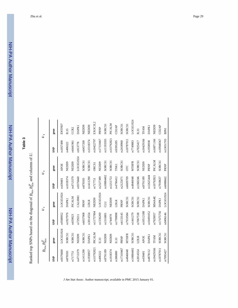
We ranked the SNPs in the BbinBbinT according to the sum of the columns, and in the first

three columns of the U matrix by their −log10(p)−values. The top 20 most significant SNPs

and their corresponding genes are listed in Table 3 under columns BbinBbinT, U1, U2, and U3,

respectively. To investigate the top SNPs and their relationship with ROI volumes in the

coefficient matrix. we retained SNPs, which are correlated with at least one ROI at a

significant level smaller than 10−6.3. For each SNP, we highlighted the locations of ROIs

with correlation at a significant level smaller than 10−6.3, which are shown in Figure 6.

There are different patterns of SNPs' effects on ROIs: i) rs10792821 (PICALM), rs9791189

(NEDD9), rs9376660 (LOC651924), and rs17310467 (PRNP) are significantly correlated

with a small number of ROIs with relative large coefficients; ii) rs4933497 (CH25H) and

rs1927976 (DAPK1) are significantly correlated with a small number of ROIs with relative

small coefficients; iii) rs1411290 (SORCS1), rs406322 (IL33), and rs1018374 (NEDD9) are

significantly correlated with a large number of ROIs with medium coefficients; iv)

rs1411290 (SORCS1), rs406322 (IL33) is significantly correlated with a large number of

ROIs with small coefficients. Figure 7 shows the heatmap of coefficients among these 10

SNPs and the ROIs on the left and right hemispheres, respectively. The ROIs are chosen

such that each ROI is significantly correlated to at least one of the 10 SNPs at a significance

level small than 10−6.3. We were able to detect some SNPs, such as rs439401 (gene APOE),

among others. The use of imaging measures as endophenotype may dramatically increase

statistical power in detecting much more informative SNPs and genes, which deserve further

investigation in Alzheimer's research. In contrast, most GWA studies often use case-control

status as the response variable, which leads to substantially power loss.

The correlation structure among imaging phenotypes and that among SNPs are characterized

by the columns in U and V, respectively. Each column of U represents a group of SNPs that

are similarly associated with a group of ROIs determined by the corresponding column of V.

The identified correlated phenotypes and genotypes largely agree with the spatial and LD

structure, which are shown in Table 3 and Figure 5. Multiple SNPs from the same gene

appear in the same columns of U. However, due to different objectives, the structure

captured by U and V may not be exactly identical to the correlation structure of imaging

phenotypes only based on the phenotypes, and the LD structure of genotypes, respectively.

5 Discussion

We have developed a Bayesian analysis GLRR to model the association between high-

dimensional responses and high-dimensional covariates with an novel application in

imaging genetic data. We have introduced a low rank regression model to approximate the

large association matrix through the standard SVD. We have used a sparse latent factor

model to more flexibly capture the complex spatial correlation structure among high-

dimensional responses. We have proposed Bayesian local hypothesis testing to identify

significant effects of genetic markers on imaging phenotypes, while controlling for multiple

comparisons. GLRR dramatically reduces the number of parameters to be sampled and

tested leading to a remarkably faster sampling scheme and effcient inference. We have

shown good finite-sample performance of GLRR in both the simulation studies and ADNI

data analysis. Our data analysis results have confirmed the important role of well-known

Zhu et al. Page 16


NIH

-PA

Author M

anuscriptN

IH-P

A A

uthor Manuscript

NIH

-PA

Author M

anuscript

genes such as APOE-∊4 in the pathology of ADNI, while highlighting other potential

candidates that warrant further investigation.

Many issues still merit further research. First, it is interesting to incorporate common variant

and rare variant genetic markers in GLRR (Bansal et al., 2010). Second, external biological

knowledge, e.g., gene pathways, may be the incorporated in the model through the use of

more delicate priors to further regularize the solution (Silver et al., 2012). Third, it is

important to consider the joint of genetic markers and environmental factors on high-

dimensional imaging phenotypes (Thomas, 2010). Fourthly, the key features of GLRR can

be adapted to more complex data structures (e.g., longitudinal, twin and family) and other

parametric and semiparametric models. For instance, for longitudinal neuroimaging data, we

may develop a GLRR to explicitly model the temporal association between high-

dimensional responses and high-dimensional covariates, while accounting for complex

temporal and spatial correction structures. Finally, it is important to combine different

imaging phenotypes calculated from other imaging modalities, such as diffusion tensor

imaging, functional magnetic resonance imaging (fMRI), and electroencephalography

(EEG), in imaging genetic studies.

Supplementary Material

Refer to Web version on PubMed Central for supplementary material.

Acknowledgments

Data used in preparation of this article were obtained from the Alzheimer's Disease Neuroimaging Initiative (ADNI) database (adni.loni.usc.edu). As such, the investigators within the ADNI contributed to the design and implementation of ADNI and/or provided data but did not participate in analysis or writing of this report. A complete listing of ADNI investigators can be found at: http://adni.loni.usc.edu/wp–content/uploads/how_to_apply/ADNI_Acknowledgement_List.pdf. We thank the Editor, the Associate Editor, and two anonymous referees for valuable suggestions, which greatly helped to improve our presentation.

The research of Drs. Zhu and Ibrahim was supported by NIH grants RR025747-01, GM70335, CA74015, P01CA142538-01, MH086633, and EB005149-01. Data collection and sharing for this project was funded by the Alzheimer's Disease Neuroimaging Initiative (ADNI) (National Institutes of Health Grant U01 AG024904) and DOD ADNI (Department of Defense award number W81XWH-12-2-0012). ADNI is funded by the National Institute on Aging, the National Institute of Biomedical Imaging and Bioengineering, and through generous contributions from the following: Alzheimer's Association; Alzheimer's Drug Discovery Foundation; BioClinica, Inc.; Biogen Idec Inc.; Bristol-Myers Squibb Company; Eisai Inc.; Elan Pharmaceuticals, Inc.; Eli Lilly and Company; F. Hoffmann-La Roche Ltd and its affiliated company Genentech, Inc.; GE Healthcare; Innogenetics, N.V.; IXICO Ltd.; Janssen Alzheimer Immunotherapy Research & Development, LLC.; Johnson & Johnson Pharmaceutical Research & Development LLC.; Medpace, Inc.; Merck & Co., Inc.; Meso Scale Diagnostics, LLC.; NeuroRx Research; Novartis Pharmaceuticals Corporation; Pfizer Inc.; Piramal Imaging; Servier; Synarc Inc.; and Takeda Pharmaceutical Company. The Canadian Institutes of Health Research is providing funds to support ADNI clinical sites in Canada. Private sector contributions are facilitated by the Foundation for the National Institutes of Health (www.fnih.org). The grantee organization is the Northern California Institute for Research and Education, and the study is coordinated by the Alzheimer's Disease Cooperative Study at the University of California, San Diego. ADNI data are disseminated by the Laboratory for Neuro Imaging at the University of Southern California.

References

Armagan, A.; Dunson, D.; Lee, J. Generalized double Pareto shrinkage. 2011. submitted

Bansal V, Libiger O, Torkamani A, Schork NJ. Statistical analysis strategies for association studies involving rare variants. Nature Reviews Genetics. 2010; 11:773–785.

Zhu et al. Page 17


NIH

-PA

Author M

anuscriptN

IH-P

A A

uthor Manuscript

NIH

-PA

Author M

anuscript

http://adni.loni.usc.edu/wpcontent/uploads/how_to_apply/ADNI_Acknowledgement_List.pdf

http://adni.loni.usc.edu/wpcontent/uploads/how_to_apply/ADNI_Acknowledgement_List.pdf

http://www.fnih.org

Benjamini Y, Hochberg Y. Controlling the false discovery rate: a practical and powerful approach to multiple testing. Journal of the Royal Statistical Society, Ser. B. 1995; 57:289–300.

Bhattacharya A, Dunson DB. Sparse Bayesian infinite factor models. Biometrika. 2011; 98:291–306. [PubMed: 23049129]

Bozdogan H. Model selection and Akaike's information criterion (AIC): the general theory and its analytical extensions. Psychometrika. 1987; 52:345–370.

Breiman L, Friedman J. Predicting multivariate responses in multiple linear regression. Journal of the Royal Statistical Society. 1997; 59:3–54.

Brown P, Vannucci M, Fearn T. Bayes Model Averaging With Selection of Regressors. Journal of the Royal Statistical Society (Series B). 2002; 64:519–536.

Cannon TD, Keller M. Endophenotypes in the genetic analyses of mental disorders. Annu Rev Clin Psychol. 2006; 40:267–290. [PubMed: 17716071]

Chen K, Chan KS, Stenseth NR. Reduced-rank stochastic regression with a sparse singular value decomposition. Journal of the Royal Statistical Society (Series B). 2012; 74:203–221.

Chiang MC, Barysheva M, Toga AW, Medland SE, Hansell NK, James MR, McMahon KL, de Zubicaray GI, Martin NG, Wright MJ, Thompson PM. BDNF gene effects on brain circuitry replicated in 455 twins. NeuroImage. 2011a; 55:448–454. [PubMed: 21195196]

Chiang MC, McMahon KL, de Zubicaray GI, Martin NG, Hickie I, Toga AW, Wright MJ, Thompson PM. Genetics of white matter development: A DTI study of 705 twins and their siblings aged 12 to 29. NeuroImage. 2011b; 54:2308–2317. [PubMed: 20950689]

Fan J, Lv J. A selective overview of variable selection in high dimensional feature space. Statistica Sinica. 2010; 20:101–148. [PubMed: 21572976]

Geweke J, Zhou G. Measuring the pricing error of the arbitrage pricing theory. The Review of Financial Studies. 1996; 9:557–587.

Hyun JW, Li YM, Gilmore JH, Lu ZH, Styner M, Zhu HT. SGPP: spatial Gaussian predictive process models for neuroimaging data. NeuroImage. 2014; 89:70–80. [PubMed: 24269800]

Izenman AJ. Reduced-rank regression for the multivariate linear model. Journal of Multivariate Analysis. 1975; 5

Kyung M, Gill J, Ghosh M. Penalized Regression, Standard Errors, and Bayesian Lassos. Bayesian Analysis. 2010; 5:369–412.

Meinshausen N, Buhlmann P. Stability selection (with discussion). Journal of the Royal Statistical Society: Series B. 2010; 72:417–473.

Müller P, Parmigiani G, Robert C, Rousseau J. Optimal sample size for multiple testing: The case of gene expression microarrays. Journal of the American Statistical Association. 2004; 99:990–1001.

Park T, Casella G. The Bayesian Lasso. Journal of the American Statistical Association. 2008; 103:681–686.

Paus T. Population neuroscience: Why and how. Human Brain Mapping. 2010; 31:891–903. [PubMed: 20496380]

Peng J, Zhu J, Bergamaschi A, Han W, Noh DY, Pollack JR, Wang P. Regularized multivariate regression for identifying master predictors with application to integrative genomics study of breast cancer. Annals of Applied Statistics. 2010; 4:53–77. [PubMed: 24489618]

Peper JS, Brouwer RM, Boomsma DI, Kahn RS, Pol HEH. Genetic influences on human brain structure: A review of brain imaging studies in twins. Human Brain Mapping. 2007; 28:464–473. [PubMed: 17415783]

Reinsel, GC.; Velu, P. Multivariate reduced-rank regression: theory and applications. Springer; New York: 1998.

Rothman AJ, Levina E, Zhu J. Sparse multivariate regression with covariance estimation. Journal of Computational and Graphical Statistics. 2010; 19:947–962. [PubMed: 24963268]

Scharinger C, Rabl U, Sitte HH, Pezawas L. Imaging genetics of mood disorders. NeuroImage. 2010; 53:810–821. [PubMed: 20156570]

Shen DG, Davatzikos C. Measuring temporal morphological changes robustly in brain MR images via 4-dimensional template warping. NeuroImage. 2004; 21:1508–1517. [PubMed: 15050575]

Zhu et al. Page 18


NIH

-PA

Author M

anuscriptN

IH-P

A A

uthor Manuscript

NIH

-PA

Author M

anuscript

Silver M, Janousova E, Hua X, Thompson PM, Montana G. Identification of gene pathways implicated in Alzheimer's disease using longitudinal imaging phenotypes with sparse regression. NeuroImage. 2012; 63:1681–1694. [PubMed: 22982105]

Thomas D. Gene–environment-wide association studies: emerging approaches. Nature Reviews Genetics. 2010; 11:259–272.

Tibshirani R. Regression shrinkage and selection via the lasso. Journal of the Royal Statistical Society (Series B). 1996; 58

Turlach BA, Venables WN, Wright SJ. Simultaneous variable selection. Technometrics. 2005; 47:349–363.

Turner JA, Smyth P, Macciardi F, Fallon J, Kennedy J, Potkin S. Imaging phenotypes and genotypes in schizophrenia. Neuroinformatics. 2006; 40:21–49. [PubMed: 16595857]

Vounou M, Nichols TE, Montana G, ADNI. Discovering genetic associations with high-dimensional neuroimaging phenotypes: A sparse reduced-rank regression approach. NeuroImage. 2010; 53:1147–1159. [PubMed: 20624472]

Wang H, Nie F, Huang H, Kim S, Nho K, Risacher SL, Saykin AJ, Shen L. Identifying quantitative trait loci via group-sparse multitask regression and feature selection: an imaging genetics study of the ADNI cohort. Bioinformatics. 2012; 28:229–237. [PubMed: 22155867]

Wang L, Dunson D. Semiparametric Bayes multiple testing: Applications to tumor data. Biometrics. 2010; 66:493–501. [PubMed: 19673866]

Yin J, Li H. A sparse conditional gaussian graphical model for analysis of genetical genomics data. Annals of Applied Statistics. 2011; 5:2630–2650. [PubMed: 22905077]

Yuan M, Ekici A, Lu Z, Monterio R. Dimension Reduction and Coefficient Estimation in Multivariate Linear Regression. Journal of the Royal Statistical Society, Ser. B. 2007; 69:329–346.

Zhu et al. Page 19


NIH

-PA

Author M

anuscriptN

IH-P

A A

uthor Manuscript

NIH

-PA

Author M

anuscript

Figure 1.

Simulation results: the box plots of five selection criteria including ,

, , AIC, and BIC against rank r from the left to the right based on

100 simulated data sets simulated from model (4) with (n, p, d) = (100, 200, 100) and the

true rank r0 = 5.

Zhu et al. Page 20


NIH

-PA

Author M

anuscriptN

IH-P

A A

uthor Manuscript

NIH

-PA

Author M

anuscript

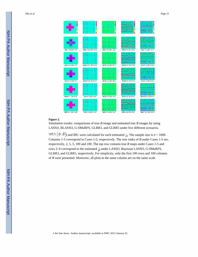
Figure 2. Simulation results: comparisons of true B image and estimated true B images by using

LASSO, BLASSO, G-SMuRFS, GLRR3, and GLRR5 under five different scenarios.

) and BIC were calculated for each estimated . The sample size is n = 1000.

Columns 1-5 correspond to Cases 1-5, respectively. The true ranks of B under Cases 1-5 are,

respectively, 2, 5, 5, 100 and 100. The top row contains true B maps under Cases 1-5 and

rows 2–6 correspond to the estimated under LASSO, Bayesian LASSO, G-SMuRFS,

GLRR3, and GLRR5, respectively. For simplicity, only the first 100 rows and 100 columns

of B were presented. Moreover, all plots in the same column are on the same scale.

Zhu et al. Page 21


NIH

-PA

Author M

anuscriptN

IH-P

A A

uthor Manuscript

NIH

-PA

Author M

anuscript

Figure 3. Comparisons of GLRR3, GLRR5, and LASSO under Cases 1-5: mean ROC curves based on

GLRR3 (red line), GLRR5 (blue line), LASSO (black line), G-SMuRFS (dottedd line) and

BLASSO (dashed line). For each case, 100 simulated data sets of size n = 100 each were

used.

Zhu et al. Page 22


NIH

-PA

Author M

anuscriptN

IH-P

A A

uthor Manuscript

NIH

-PA

Author M

anuscript

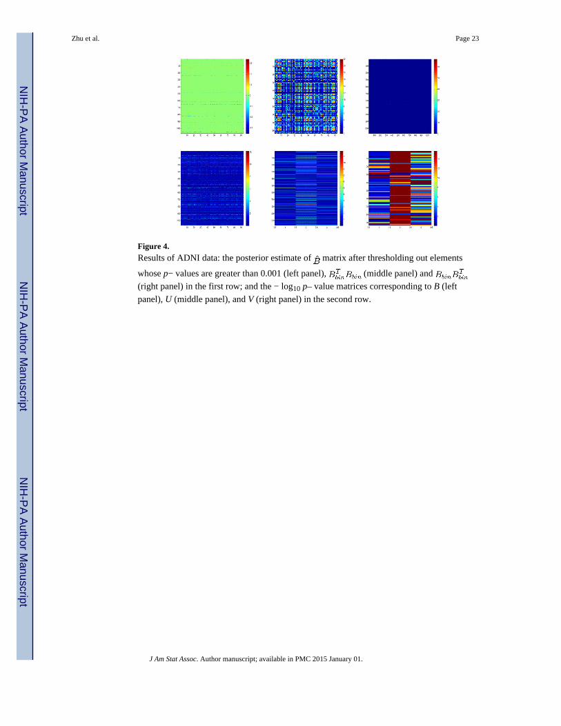
Figure 4. Results of ADNI data: the posterior estimate of matrix after thresholding out elements

whose p− values are greater than 0.001 (left panel), (middle panel) and

(right panel) in the first row; and the − log10 p– value matrices corresponding to B (left

panel), U (middle panel), and V (right panel) in the second row.

Zhu et al. Page 23


NIH

-PA

Author M

anuscriptN

IH-P

A A

uthor Manuscript

NIH

-PA

Author M

anuscript

Figure 5.

Results of ADNI data: the top 20 ROIs based on and the first 3 columns of V. The

sizes of the dots represent the rank of the ROIs.

Zhu et al. Page 24


NIH

-PA

Author M

anuscriptN

IH-P

A A

uthor Manuscript

NIH

-PA

Author M

anuscript

Figure 6. Results of ADNI data: at a −log10(p) significance level greater than 6.3, the top row depicts

the locations of ROIs that are correlated with SNPs rs10792821 (PICALM), rs9791189

(NEDD9), rs9376660 (LOC651924), rs17310467 (PRNP), rs4933497 (CH25H),

respectively; the bottom row shows the ROIs correlated with SNPs rs1927976 (DAPK1),

rs1411290 (SORCS1), rs406322 (IL33), rs1018374 (NEDD9), and rs439401 (APOE). The

sizes of the dots represent the absolute magnitudes of the regression coefficients.

Zhu et al. Page 25


NIH

-PA

Author M

anuscriptN

IH-P

A A

uthor Manuscript

NIH

-PA

Author M

anuscript

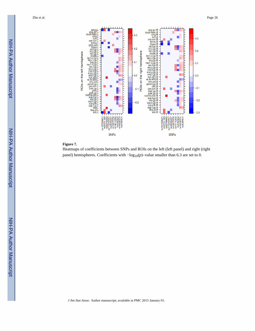
Figure 7. Heatmaps of coefficients between SNPs and ROIs on the left (left panel) and right (right

panel) hemispheres. Coefficients with −log10(p)–value smaller than 6.3 are set to 0.

Zhu et al. Page 26


NIH

-PA

Author M

anuscriptN

IH-P

A A

uthor Manuscript

NIH

-PA

Author M

anuscript

NIH

-PA

Author M

anuscriptN

IH-P

A A

uthor Manuscript

NIH

-PA

Author M

anuscript

Zhu et al. Page 27

Table 1

Empirical comparison of GLRR3, GLRR5, LASSO, BLASSO and G-SMuRFS under Cases 1-5 based on the

five selection criteria. The means and standard deviations of these criteria are also calculated and their

standard deviations are presented in parentheses. Moreover, UN denotes the unstructured B.

Case/(p, d, n)/X B/r 0 Method MEN PEN R 2 AIC BIC

1 (100,100,100) Continuous “+” 2 LASSO 6.21 (0.83) 3.98 (0.73) 89.50 (2.03) 9.54 (0.08) 12.45 (0.24)

BLASSO 4.63 (0.48) 4.19 (0.57) 92.09 (1.13) 10.82 (0.08) 18.02 (0.07)

G-SMuRFS 5.74 (0.65) 1.88 (0.30) 94.62 (0.71) 10.01 (0.10) 17.22 (0.10)

GLRR3 11.81 (10.96) 3.17 (7.35) 94.71 (7.34) 8.27 (0.47) 8.70 (0.47)

GLRR5 6.81 (6.87) 2.14 (3.69) 94.73 (3.72) 8.16 (0.31) 8.88 (0.31)

2 (200,100,100) Continuous UΔV 5 LASSO 26.64 (2.15) 1.26 (1.49) 97.37 (6.01) 11.94 (0.77) 18.25 (0.93)

BLASSO 22.38 (1.63) 1.24 (0.21) 98.55 (0.33) 13.39 (0.41) 27.78 (0.41)

G-SMuRFS 21.87 (1.69) 1.11 (0.11) 98.20 (0.07) 9.95 (0.10) 24.38 (0.24)

GLRR3 31.56 (6.56) 14.60 (9.24) 83.77 (9.75) 12.88 (0.61) 13.53 (0.61)

GLRR5 21.69 (1.87) 0.36 (1.93) 98.54 (2.22) 8.90 (0.47) 8.88 (0.47)

3 (400,100,100) SNPs UΔV 5 LASSO 50.41 (12.00) 50.87 (11.94) 19.59 (7.78) 12.81 (0.15) 13.66 (0.23)

BLASSO 25.57 (0.02) 10.08 (2.04) 93.24 (3.29) 15.69 (0.39) 43.53 (0.39)

G-SMuRFS 24.28 (0.02) 10.27 (2.01) 91.69 (4.01) 16.96 (0.01) 42.80 (0.01)

GLRR3 20.23 (4.25) 21.39 (13.96) 76.74 (14.20) 11.86 (0.60) 12.93 (0.60)

GLRR5 13.64 (7.88) 4.07 (7.77) 93.60 (7.97) 10.19 (0.60) 11.99 (0.60)

4 (200,100,100) Continuous UN 100 LASSO 22.16 (1.93) 1.27 (1.49) 94.40 (6.16) 12.45 (0.88) 19.11 (1.12)

BLASSO 19.44 (1.16) 1.22 (0.21) 98.32 (0.74) 13.21 (0.79) 27.63 (0.79)

G-SMuRFS 15.00 (1.44) 1.10 (0.01) 98.40 (0.08) 9.74 (0.11) 24.16 (0.11)

GLRR3 18.32 (1.53) 5.16 (0.64) 93.93 (0.73) 12.20 (0.04) 12.85 (0.04)

GLRR5 16.02 (1.59) 4.30 (0.56) 94.26 (0.71) 12.14 (0.03) 13.22 (0.03)

5 (400,100,100) SNPs UN 100 LASSO 39.14 (12.93) 39.11 (12.95) 24.53 (9.53) 14.60 (0.12) 17.22 (0.62)

BLASSO 22.43 (1.13) 12.07 (0.03) 89.31 (0.24) 15.60 (0.35) 41.44 (0.35)

G-SMuRFS 18.58 (0.02) 12.27 (0.01) 88.69 (0.01) 16.96 (0.01) 42.21 (0.01)

GLRR3 19.88 (0.01) 20.01 (0.03) 77.15 (0.04) 13.56 (0.00) 14.64 (0.00)

GLRR5 17.87 (0.01) 17.98 (0.03) 77.81 (0.04) 13.65 (0.00) 14.45 (0.00)


NIH

-PA

Author M

anuscriptN

IH-P

A A

uthor Manuscript

NIH

-PA

Author M

anuscript

Zhu et al. Page 28

Table 2

Ranked top ROIs based on the diagonal of and columns of V.

V 1 V 2 V 3

hiopp.R caud.neuc.L sup.t.gy.L sup.p.lb.L

hiopp.L caud.neuc.R sup.t.gy.R pstc.gy.L

amyg.R post.limb.L mid.t.gy.R sup.o.gy.L

unc.L post.limb.R hiopp.R prec.L

subtha.nuc.R glob.pal.R mid.t.gy.L sup.p.lb.R

sup.t.gy.R ant.caps.R hiopp.L pec.R

amyg.L glob.pal.L amyg.R sup.o.gy.R

sup.t.gy.L putamen. L lat.ve.R prec.gy.L

lat.ve.R putamen. R inf.t.gy.R pstc.gy.R

nuc.acc.L ant.caps.L subtha.nuc.R prec.gy.R

lat.ve.L thal.R amyg.L me.f.gy.L

mid.t.gy.L thal.L unc.L mid.f.gy.R

insula.L tmp.pl.R lat.ve.L ang.gyr.L

sup.f.gy.L subtha.nuc.L inf.f.gy.R sup.f.gy.L

insula.R per.cort.L lat.f-o.gy.L fornix.L

mid.t.gy.R tmp.pl.L parah.gy.L occ.pol.L

mid.f.gy.L subtha.nuc.R inf.t.gy.L ang.gyr.R

unc.R per.cort.R parah.gy.R cun.L

inf.t.gy.R nuc.acc.L nuc.acc.L occ.pol.R

inf.f.gy.R inf.t.gy.R insula.L mid.f.gy.L


NIH

-PA

Author M

anuscriptN

IH-P

A A

uthor Manuscript

NIH

-PA

Author M

anuscript

Zhu et al. Page 29

Tab

le 3

Ran

ked

top

SNPs

bas

ed o

n th

e di

agon

al o

f a

nd c

olum

ns o

f U

.

U 1

U 2

U 3

SNP

gene

SNP

gene

SNP

gene

SNP

gene

rs93

7666

0L

OC

6519

24rs

9389

952

LO

C65

1924

rs43

9401

APO

Ers

1057

490

EN

TPD

7

rs87

8183

SOR

CS1

rs19

2797

6D

APK

1rs

1018

374

NE

DD

9rs

4063

22IL

33

rs71

7751

SOR

CS1

rs65

9023

PIC

AL

Mrs

4713

379

NE

DD

9rs

6441

961

CC

R2

rs47

1337

9N

ED

D9

rs72

9211

CA

LH

M1

rs93

7666

0L

OC

6519

24rs

9137

78D

APK

1

rs14

1129

0SO

RC

S1rs

6037

908

PRN

Prs

8781

83SO

RC

S1rs

6457

200

NE

DD

9

rs19

3005

7D

APK

1rs

3014

554

LD

LR

rs14

1129

0SO

RC

S1rs

1O18

374

NE

DD

9

rs1O

7928

21PI

CA

LM

rs11

7579

04N

ED

D9

rs71

7751

OR

CS1

rs10

4227

97E

XO

C3L

2

rs40

6322

IL33

rs13

3626

9L

OC

6519

24rs

2327

389

NE

DD

9rs

1731

0467

PRN

P

rs97

9118

9N

ED

D9

rs13

1680

1C

LU

rs10

8844

02SO

RC

S1rs

1119

3593

SOR

CS1

rs10

1837

4N

ED

D9

rs74

4970

NE

DD

9rs

1251

753

SOR

CS1

rs1O

7928

21PI

CA

LM

rs38

6880

IL33

rs17

9989

8L

DL

Rrs

4796

412

TN

K1

rs93

9528

5C

D2A

P

rs17

3104

67PR

NP

rs61

3314

5PR

NP

rs21

2507

1SO

RC

S1rs

2418

960

SOR

CS1

rs48

4604

8M

TH

FRrs

7910

584

SOR

CS1

rs66

0970

9O

TC

rs10

7870

11SO

RC

S1

rs10

8844

02SO

RC

S1rs

1441

279

SOR

CS1

rs48

4604

8M

TH

FRrs

7749

883

LO

C65

1924

rs30

1455

4L

DL

Rrs

7067

538

SOR

CS1

rs13

6024

6SO

RC

S1rs

7025

417

IL33

rs43

9401

APO

Ers

1051

2188

DA

PK1

rs97

9118

9N

ED

D9

rs10

4291

66T

FAM

rs48

7811

2D

APK

1rs

1049

1052

SOR

CS1

rs12

6254

44PR

NP

rs19

5893

8D

APK

1

rs10

4291

66T

FAM

rs79

2905

7M

S4A

4Ers

1079

2821

PIC

AL

Mrs

1687

1166

NE

DD

9

rs10

7870

11SO

RC

S1rs

1747

5756

DA

PK1

rs79

1863

7SO

RC

S1rs

1094

8367

CD

2AP

rs70

9542

7SO

RC

S1rs

9496

146

LO

C65

1924

rs60

8866

2PR

NP

rs13

0317

03B

IN1


Documents

NIH Public Access Zhaohua Lu Joseph G. Ibrahim Alzheimer's ... · Neuroimaging Phenotypes and Genetic Markers Hongtu Zhu , Zakaria Khondker , Zhaohua Lu , Joseph G. Ibrahim , and