NICE: Non-linear Independent Components Estimation

Laurent Dinh David Krueger Yoshua Bengio∗Departement d’informatique et de recherche operationnelle

Universite de MontrealMontreal, QC H3C 3J7

Abstract

We propose a deep learning framework for modeling complex high-dimensional densities via Non-linear Independent Component Estimation (NICE). It is based on the idea that a good representationis one in which the data has a distribution that is easy to model. For this purpose, a non-lineardeterministic transformation of the data is learned that maps it to a latent space so as to make thetransformed data conform to a factorized distribution, i.e., resulting in independent latent variables.We parametrize this transformation so that computing the determinant of the Jacobian and inverseJacobian is trivial, yet we maintain the ability to learn complex non-linear transformations, via acomposition of simple building blocks, each based on a deep neural network. The training criterionis simply the exact log-likelihood, which is tractable, and unbiased ancestral sampling is also easy.We show that this approach yields good generative models on four image datasets and can be usedfor inpainting.

1 Introduction

One of the central questions in unsupervised learning is how to capture complex data distributions that have unknownstructure. Deep learning approaches (Bengio, 2009) rely on the learning of a representation of the data that wouldcapture its most important factors of variation. This raises the question: what is a good representation? Like inrecent work (Kingma and Welling, 2014; Rezende et al., 2014; Ozair and Bengio, 2014), we take the view that a goodrepresentation is one in which the distribution of the data is easy to model. In this paper, we consider the specialcase where we ask the learner to find a transformation h = f(x) of the data into a new space such that the resultingdistribution factorizes, i.e., the components hd are independent:

pH(h) =∏d

pHd(hd).

We can think of the transformation f as acting on the distribution by twisting and folding the space so as to achieve thatobjective. In particular, if we think geometrically about a low-dimensional manifold near which the data distributionconcentrates, the learned transformation tries to flatten the manifold. A flat manifold has the property that if twovectors v1 and v2 are on it, then a convex combination αv1 + (1− α)v2 is likely to be on the manifold as well. In thispaper, we can observe such flattening as found in (Bengio et al., 2013) with stacked autoencoders and RBMs. Indeed,if the components of h are independent, it means that if hd ∈ Ad (whereAd is an interval) is likely under pHd

(hd), thenso are all the points in the volume A1×A2× . . ., which thus forms a convex set of probable configuration. In additionto flattening the manifold to separate it from the ambiant space, using a marginally independent prior also puts pres-sure on the transformation f to stretch the space non-linearly in order to make the different hd marginally independent.

∗Yoshua Bengio is a CIFAR Senior Fellow.

1

arX

iv:1

410.

8516

v1 [

cs.L

G]

30

Oct

201

4

The proposed training criterion is directly derived from the log-likelihood. More specifically, we consider a change ofvariable h = f(x), which assumes that f is invertible and the dimension of h is the same as the dimension of x, inorder to fit a distribution pH . The change of variable rule gives us:

pX(x) = pH(f(x))|det∂f(x)

∂x|. (1)

where ∂f(x)∂x is the Jacobian matrix of function f at x. In this paper, we choose f such that the determinant of the

Jacobian is trivially obtained. Moreover, its inverse f−1 is also trivially obtained, allowing us to sample from pX(x)easily as follows:

h ∼ pH(h)

x = f−1(h). (2)

A key novelty of this paper is the design of such a transformation f that yields these two properties of “easy determinantof the Jacobian” and “easy inverse”, while allowing us to have as much capacity as needed in order to learn complextransformations. The core idea behind this is that we can split x into two blocks (x1, x2) and apply as building blockthe transformation from (x1, x2) to (y1, y2) of the form:

y1 = x1

y2 = x2 +m(x1) (3)

where m is an arbitrarily complicated function. This building block has a unit Jacobian determinant for any m and istrivially invertible since:

x1 = y1

x2 = y2 −m(y1). (4)

The details, surrounding discussion and experimental results are developed below.

2 Issues of training with continuous data

We consider the problem of learning a density from a parametric family of densities {pθ, θ ∈ Θ} over finite datasetD of N examples, each living in a space X ; typically X = RD. In this setting there is no natural upper limit on thelog-likelihood that can be achieved (unlike for discrete data). As a result, several issues can arise from naive attemptsat maximizing likelihood. For instance, as highlighted in (Bishop, 2006), a fully parametrized a mixture of gaussianscan use one of its mixture component to model one of the datapoints with arbitrary precision, arbitrarily raising thetraining log-likelihood. As the test log-likelihood of such a model is often correspondingly low, this can be consideredan overfitting issue. However, we will show two cases where similar singularity issues arise and generalize to test data.

Continuous data is recorded with a finite amount of precision, generally much less than present-day computerprecision. For the purposes of this paper, we can consider the level of precision represented on the computer ascontinuous, and coarser data as “quantized”. This kind of quantization allows the log-likelihood to be increasedarbitrarily not only on the training set but also on the test set. For example, one can achieve this by building a mixtureof Gaussians covering every quantum with infinite precision.

Introducing noise can counter this effect. For example, we can stochastically dequantize the data by introducing auniform noise to reflect the uncertainty introduced by quantization1. Moreover, such noise added to the train and testsets introduces an upper bound on log-likelihood in expectation. Treating the data as discrete also results in an upperbound, but at the price of differentiability.

Data preprocessing is a widespread practice in machine learning. It can provide a more useful signal to the machinelearning algorithm than the raw data and as long as the preprocessing is invertible it remains very relevant to

1This is not the exact procedure but it is less cumbersome than to reverse-engineer the more complex quantization process.

2

H

X

(a) Inference

H

X

(b) Sampling

H

XO XH

(c) Inpainting

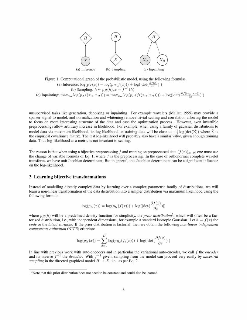
Figure 1: Computational graph of the probabilistic model, using the following formulas.(a) Inference: log(pX(x)) = log(pH(f(x))) + log(|det(∂f(x)∂x )|)

(b) Sampling: h ∼ pH(h), x = f−1(h)

(c) Inpainting: maxxHlog(pX((xO, xH))) = maxxH

log(pH(f((xO, xH)))) + log(|det(∂f((xO,xH))∂x )|)

unsupervised tasks like generation, denoising or inpainting. For example wavelets (Mallat, 1999) may provide asparser signal to model, and normalization and whitening remove trivial scaling and correlation allowing the modelto focus on more interesting structure of the data and ease the optimization process. However, even invertiblepreprocessings allow arbitrary increase in likelihood. For example, when using a family of gaussian distributions tomodel data via maximum-likelihood, its log-likelihood on training data will be close to − 1

2 log(det(Σ)) where Σ isthe empirical covariance matrix. The test log-likeihood will probably also have a similar value, given enough trainingdata. Thus log-likelihood as a metric is not invariant to scaling.

The reason is that when using a bijective preprocessing f and training on preprocessed data (f(x))x∈D, one must usethe change of variable formula of Eq. 1, where f is the preprocessing. In the case of orthonormal complete wavelettransform, we have unit Jacobian determinant. But in general, this Jacobian determinant can be a significant influenceon the log-likelihood.

3 Learning bijective transformations

Instead of modelling directly complex data by learning over a complex parametric family of distributions, we willlearn a non-linear transformation of the data distribution into a simpler distribution via maximum likelihood using thefollowing formula:

log(pX(x)) = log(pH(f(x))) + log(|det(∂f(x)

∂x)|)

where pH(h) will be a predefined density function for simplicity, the prior distribution2, which will often be a fac-torized distribution, i.e., with independent dimensions, for example a standard isotropic Gaussian. Let h = f(x) thecode or the latent variable. If the prior distribution is factorial, then we obtain the following non-linear independentcomponents estimation (NICE) criterion:

log(pX(x)) =

D∑d=1

log(pHd(fd(x))) + log(|det(

∂f(x)

∂x)|)

In line with previous work with auto-encoders and in particular the variational auto-encoder, we call f the encoderand its inverse f−1 the decoder. With f−1 given, sampling from the model can proceed very easily by ancestralsampling in the directed graphical model H → X , i.e., as per Eq. 2.

2Note that this prior distribution does not need to be constant and could also be learned

3

= ykeygycipher

m

xkeyxplain

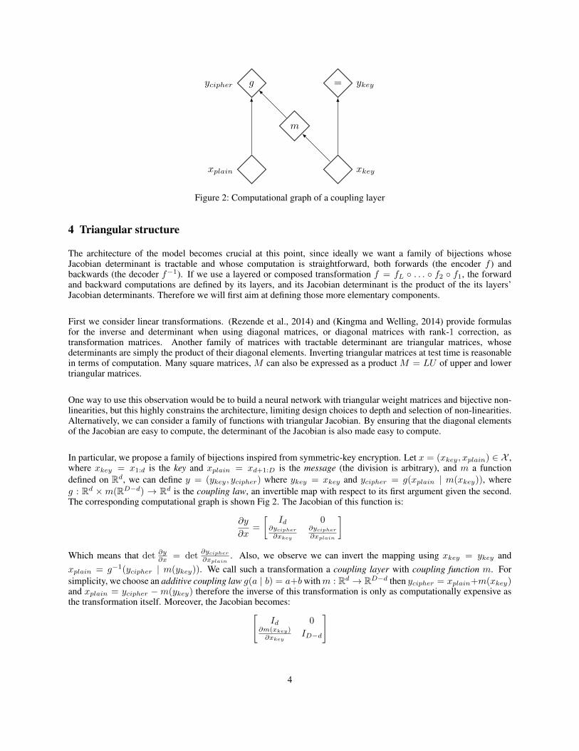
Figure 2: Computational graph of a coupling layer

4 Triangular structure

The architecture of the model becomes crucial at this point, since ideally we want a family of bijections whoseJacobian determinant is tractable and whose computation is straightforward, both forwards (the encoder f ) andbackwards (the decoder f−1). If we use a layered or composed transformation f = fL ◦ . . . ◦ f2 ◦ f1, the forwardand backward computations are defined by its layers, and its Jacobian determinant is the product of the its layers’Jacobian determinants. Therefore we will first aim at defining those more elementary components.

First we consider linear transformations. (Rezende et al., 2014) and (Kingma and Welling, 2014) provide formulasfor the inverse and determinant when using diagonal matrices, or diagonal matrices with rank-1 correction, astransformation matrices. Another family of matrices with tractable determinant are triangular matrices, whosedeterminants are simply the product of their diagonal elements. Inverting triangular matrices at test time is reasonablein terms of computation. Many square matrices, M can also be expressed as a product M = LU of upper and lowertriangular matrices.

One way to use this observation would be to build a neural network with triangular weight matrices and bijective non-linearities, but this highly constrains the architecture, limiting design choices to depth and selection of non-linearities.Alternatively, we can consider a family of functions with triangular Jacobian. By ensuring that the diagonal elementsof the Jacobian are easy to compute, the determinant of the Jacobian is also made easy to compute.

In particular, we propose a family of bijections inspired from symmetric-key encryption. Let x = (xkey, xplain) ∈ X ,where xkey = x1:d is the key and xplain = xd+1:D is the message (the division is arbitrary), and m a functiondefined on Rd, we can define y = (ykey, ycipher) where ykey = xkey and ycipher = g(xplain | m(xkey)), whereg : Rd ×m(RD−d) → Rd is the coupling law, an invertible map with respect to its first argument given the second.The corresponding computational graph is shown Fig 2. The Jacobian of this function is:

∂y

∂x=

[Id 0

∂ycipher

∂xkey

∂ycipher

∂xplain

]Which means that det ∂y∂x = det

∂ycipher

∂xplain. Also, we observe we can invert the mapping using xkey = ykey and

xplain = g−1(ycipher | m(ykey)). We call such a transformation a coupling layer with coupling function m. Forsimplicity, we choose an additive coupling law g(a | b) = a+bwithm : Rd → RD−d then ycipher = xplain+m(xkey)and xplain = ycipher −m(ykey) therefore the inverse of this transformation is only as computationally expensive asthe transformation itself. Moreover, the Jacobian becomes:[

Id 0∂m(xkey)∂xkey

ID−d

]

4

Therefore, an additive coupling layer transformation has a unit Jacobian determinant and a trivial inverse. One couldalso choose other types of coupling like multiplicative coupling law g(a | b) = a � b, b 6= 0 or affine coupling lawg(a, b) = a� b1 + b2, b1 6= 0 if m : Rd → RD−d × RD−d.

Since a coupling layer leaves part of its input unchanged, we exchange the role of message and key in alternatinglayers, so that the composition of two coupling layers modifies every dimension. Examining the Jacobian, we observethat at least three coupling layers are necessary to allow all dimensions to influence one another. We include a diagonalscaling matrix S as the top layer, which multiplies the d-th ouput value by Sdd, resulting in the following simplifiedversion of the NICE criterion:

log(pX(x)) =

D∑i=d

log(pHd(fd(x))) + log(Sdd)

We can interpret these scaling factors as a kind of spectrum, showing how much variation is present in each of thelatent dimensions (the larger Sdd is, the less important the dimension d is). The important dimensions of the spectrumcan be viewed as a manifold learned by the algorithm. The prior term tries to make Sdd small (trying minimize entropyof H), while the determinant term logSdd prevents Sdd from ever reaching 0.

5 Related methods

Significant advances have been made in generative models. Undirected graphical models like deep Boltzmannmachines (DBM) (Salakhutdinov and Hinton, 2009) were for a while the most successful due to efficient approximateinference and learning techniques that these models allowed. However, these models require MCMC sampling proce-dure for training and sampling and these MCMCs are generally slowly mixing when the target distribution has sharpmodes. In addition, the log-likelihood is intractable, and the best known estimation procedure, annealed importancesampling (AIS) (Salakhutdinov and Murray, 2008), might yield an overly optimistic evaluation (Roger Grosse andSalakhutdinov, 2013).

Directed graphical models lack the conditional independence structure that allows DBMs efficient inference.However, recent advances in the framework of variational auto-encoders (VAE) - which come under a variety ofnames and variants (Kingma and Welling, 2014; Rezende et al., 2014; Mnih and Gregor, 2014; Gregor et al., 2014)- allowed effective approximate inference for training. In constrast with the NICE model, these approaches usea stochastic encoder Q(h|x) and an imperfect decoder, and add a reconstruction term, logP (x|h), to the cost, toensure that the decoder approximately inverts the encoder. This injects noise into the auto-encoder loop, since his sampled from Q(h|x), which is a variational approximation to the true posterior, P (h|x). The cost functionalso involves a term for maximizing the entropy of Q(h|x), which is not required here. The resulting trainingcriterion is the variational lower bound on the log-likelihood of the data. The generally fast ancestral samplingtechnique that directed graphical models provide make these models appealing. Moreover, the importance samplingestimator of the log-likelihood is guaranteed not to be optimistic in expectation. However, using a lower boundcriterion might yield a suboptimal solution with respect to the true log-likelihood. Furthermore, with reconstructionerror typically being non-negligeable, the “correct” generative model always wants to add iid noise at the lastgenerative step, which in the case of images, speech, or text, would often make for unnatural-looking samples.In practice, this issue can be avoided by taking the expectation of P (x|h) as a sample, instead of actually sam-pling the distribution. The use of a deterministic decoder can be motivated as a rigorous way of eliminating such noise.

The NICE criterion is very similar to the criterion of the variational autoencoder. More specifically, as the transforma-tion and its inverse can be seen as a perfect autoencoder pair (Bengio, 2014), the reconstruction term is a constant thatcan be ignored. This leaves the Kullback-Leibler divergence term of the variational criterion; log(pH(f(x))) can beseen as the prior term, which forces the code to be likely with respect to the prior distribution, and log(|det ∂f(x)∂x |) canbe seen as the entropy term. This entropy term reflects the local volume expansion around the data (for the encoder),which translates into contraction in the decoder f−1. In a similar fashion, the entropy term in the variational criterionencourages the approximate posterior distribution to occupy volume, which also translates into contraction from thedecoder. The drawback of perfect reconstruction/bijectivity is that we also have to model the noise, which is generally

5

handled by the conditional model P (x|h) in these graphical models.

We also observe that by combining the variational criterion with the reparametrization trick, (Kingma and Welling,2014) is effectively maximizing the joint log-likelihood of the pair (x, ε) in a NICE model with two affine couplinglayers (where ε is the auxiliary noise variable).

Another interesting comparison is with the work of (Ozair and Bengio, 2014), which also considers a deterministicencoder, but with discrete input and latent variables, which is not always invertible. This can be interpreted as a hashfunction, whereas the transformation used in this paper can be seen as perfect hash function, i.e. injective. Hencethey have to learn a decoder which is not going to be perfect in practice. They also have to confront the challenges ofgradient-based optimization of discrete functions, which do not arise in the continuous case.

The change of variable formula for probability density functions is prominently used in inverse transform sampling(which is effectively the procedure used for sampling here). Independent component analysis (ICA) (Hyvarinen andOja, 2000), and more specifically its maximum likelihood formulation, learn an orthogonal transformation of thedata, necessitating a costly orthogonalization proceedure between parameter updates. Learning a richer family oftransformations was proposed in (Bengio, 1991), but the proposed class of transformations, neural networks, lacksthe structure to make the inference and optimization practical.

(Rippel and Adams, 2013) reintroduces this idea but drops the bijectivity constraint but has to rely on a compositeproxy to optimize the log-likelihood. A more principled proxy of log-likelihood, the variational lower bound, isused more successfully in (Kingma and Welling, 2014) and (Rezende et al., 2014). Generative adversarial networks(GAN) (Goodfellow et al., 2014) also train a generative model to transform a simple (e.g. factorial) distribution intothe data distribution, but do not require an encoder that goes in the other direction. GAN sidesteps the difficulties ofinference by learning a secondary deep network that discriminates between GAN samples and data. This classifierthen provides a training signal to the GAN generative model, telling it how to change its output in order for it to beundistinguishable from the training data.

Like the variational auto-encoders, the NICE model uses an encoder to avoid the difficulties of inference, but itsencoding is deterministic. The log-likelihood is tractable and the training procedure does not require any sampling(apart from dequantizing the data). The triangular structure used in NICE to obtain tractability is also present inanother tractable density model, the neural autoregressive density estimator (NADE) (Larochelle and Murray, 2011),inspired by (Bengio and Bengio, 2000). Indeed, the adjacency matrix in the NADE directed graphical model is strictlytriangular. However the element-by-element autoregressive scheme of NADE make the ancestral sampling procedurecomputationally expensive for generative tasks on high-dimensional data, such as image data. A NICE model usingone coupling layer can be seen as a block version of NADE with two blocks.

6 Experiments

6.1 Log-likelihood and generation

We train NICE on MNIST (LeCun and Cortes, 1998), the Toronto Face Dataset 3 (TFD) (Susskind et al., 2010), theStreet View House Numbers dataset (SVHN) (Netzer et al., 2011) and CIFAR-10 (Krizhevsky, 2010). As mentionedearlier we use a dequantized version of the data, and the data is rescaled to be in [0, 1]D after dequantization. Thesetwo steps correspond to the following preprocessing:

x =255

256x+ u (5)

where u ∼ U([0, 256−1]). CIFAR-10 is normalized to be in [−1, 1]D.

3We train on unlabeled data for this dataset.

6

The architecture for MNIST and SVHN used is a stack of four coupling layers with a diagonal positive scaling for thelast stage, parametrized exponentially:

Sdd = eadd . (6)We partition the input space between key and message by separating odd and even components. The couplingfunction used for each coupling layer is a deep rectified network with linear output units. For MNIST and SVHN,we stack four such coupling layers, using 392 − 1000 − 1000 − 1000 − 1000 − 1000 − 392 units4 for MNIST and1536−2000−2000−1536 for SVHN. We use eight coupling layers that have (in order) 3−3−2−2−1−1−1−1hidden layers with 2000 hidden units for TFD, and 1−1−3−3−2−2−1−1 hidden layers with 2400 units for CIFAR.

A standard logistic distribution is used as prior for MNIST and TFD, as its negative log-likelihood function correspondto the smooth L1 penalty (Hyvarinen et al., 2009) x 7→ log cosh(x). A standard normal distribution is used as priorfor SVHN and CIFAR-10.

The models are training with RMSProp (Tieleman and Hinton, 2012) with learning rate 10−3 exponentially decreasingto 10−4 with exponential decay of 1.0005, that is a learning rate:

α = max(1.0005−e × 10−3, 10−4)

Where e is the number of epochs. For CIFAR-10 the learning rate goes from 2 × 10−4 to 10−5 with the same decayrate. The decay coefficient of RMSProp is β = 0.95 and maximum scaling of 100. The momentum is initially ρ = 0and becomes ρ = 0.5 at the fifth epoch, giving the update rule:

g2t+1 =βg2t + (1− β)∂L

∂θ

2

µt+1 =ρµt − αmin((g2t+1)−1, 100)∂L

∂θθt+1 =θt + µt+1

The operations are elementwise, θ is the parameter and L is the loss function, here negative log-likleihood. We selectthe best model in terms of validation log-likelihood after 1500 epochs, or using early stopping.

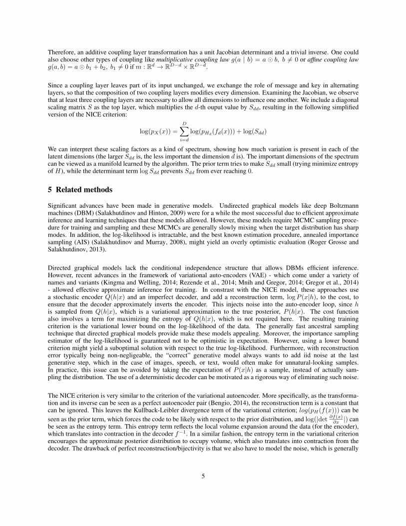
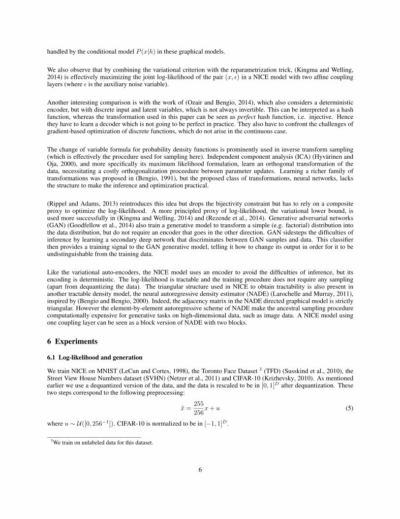
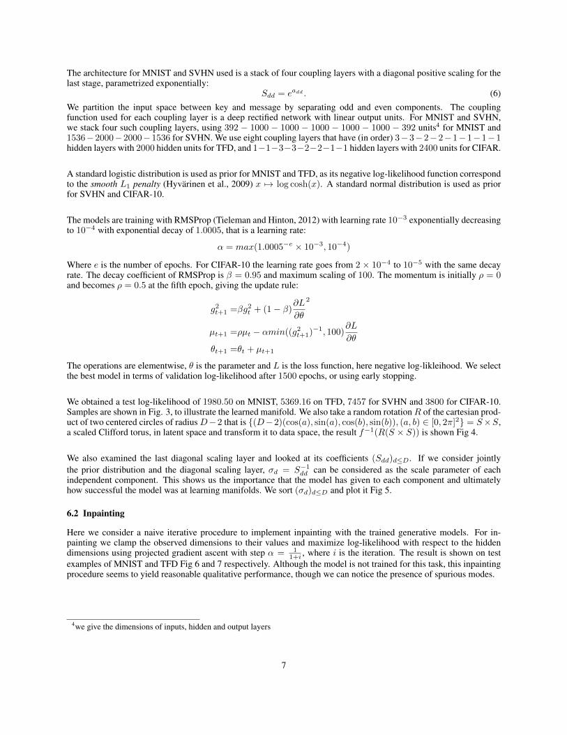
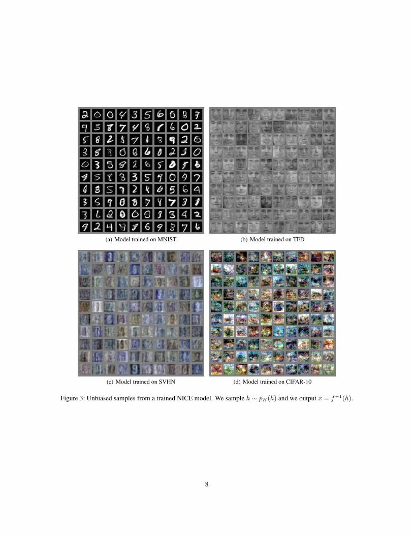
We obtained a test log-likelihood of 1980.50 on MNIST, 5369.16 on TFD, 7457 for SVHN and 3800 for CIFAR-10.Samples are shown in Fig. 3, to illustrate the learned manifold. We also take a random rotationR of the cartesian prod-uct of two centered circles of radius D−2 that is {(D−2)(cos(a), sin(a), cos(b), sin(b)), (a, b) ∈ [0, 2π]2} = S×S,a scaled Clifford torus, in latent space and transform it to data space, the result f−1(R(S × S)) is shown Fig 4.

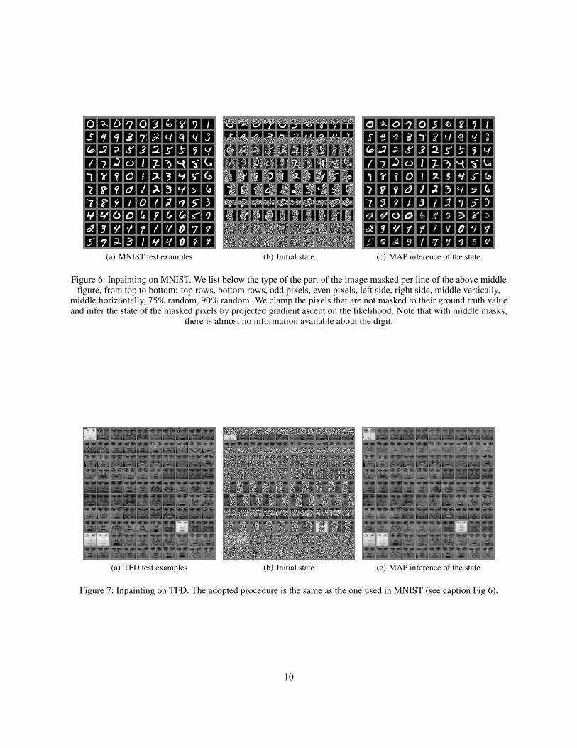
We also examined the last diagonal scaling layer and looked at its coefficients (Sdd)d≤D. If we consider jointlythe prior distribution and the diagonal scaling layer, σd = S−1dd can be considered as the scale parameter of eachindependent component. This shows us the importance that the model has given to each component and ultimatelyhow successful the model was at learning manifolds. We sort (σd)d≤D and plot it Fig 5.

6.2 Inpainting

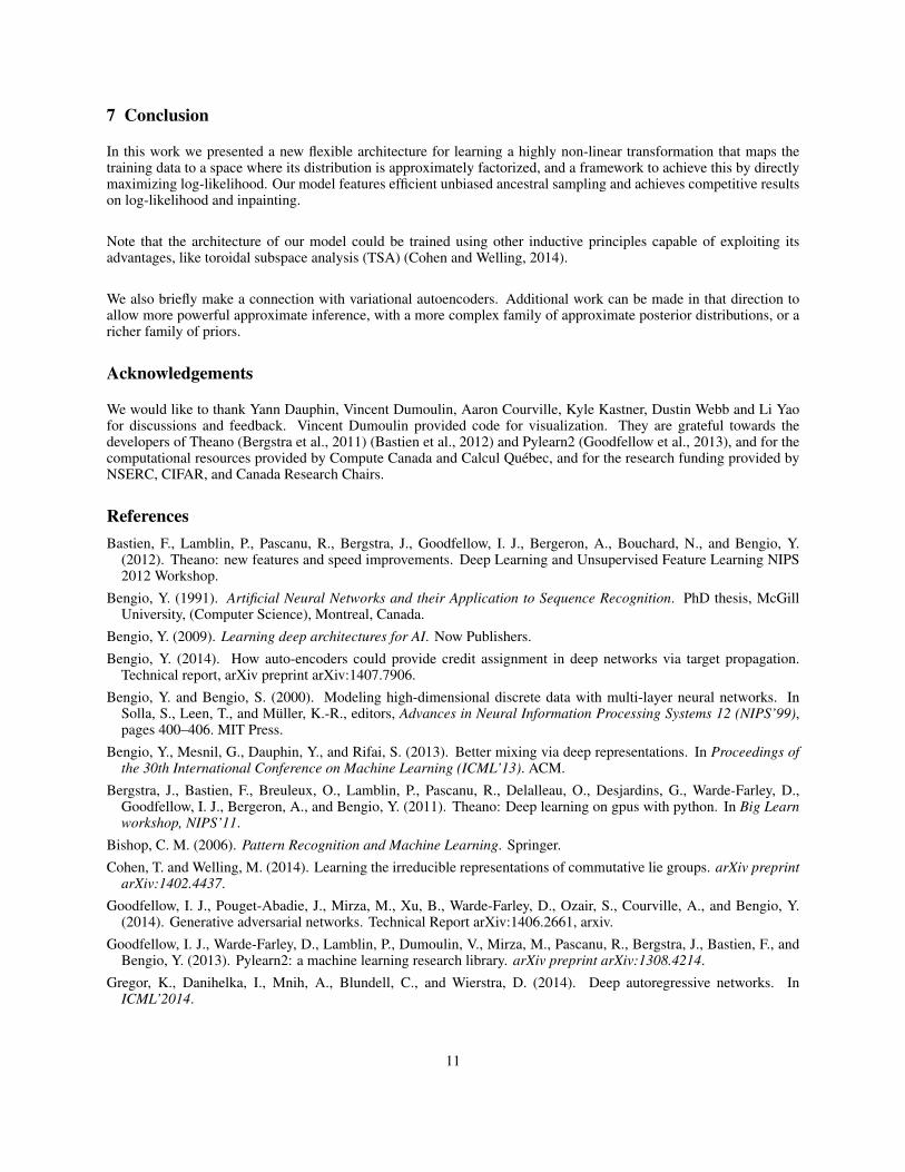
Here we consider a naive iterative procedure to implement inpainting with the trained generative models. For in-painting we clamp the observed dimensions to their values and maximize log-likelihood with respect to the hiddendimensions using projected gradient ascent with step α = 1

1+i , where i is the iteration. The result is shown on testexamples of MNIST and TFD Fig 6 and 7 respectively. Although the model is not trained for this task, this inpaintingprocedure seems to yield reasonable qualitative performance, though we can notice the presence of spurious modes.

4we give the dimensions of inputs, hidden and output layers

7

(a) Model trained on MNIST (b) Model trained on TFD

(c) Model trained on SVHN (d) Model trained on CIFAR-10

Figure 3: Unbiased samples from a trained NICE model. We sample h ∼ pH(h) and we output x = f−1(h).

8

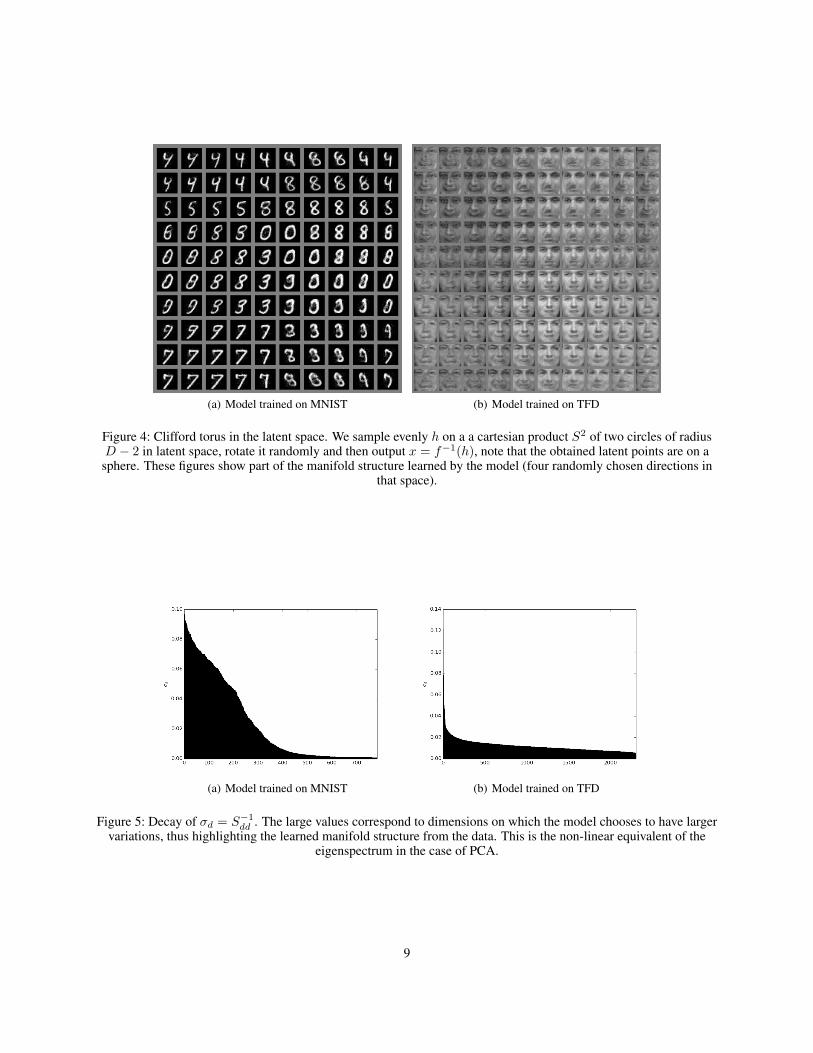
(a) Model trained on MNIST (b) Model trained on TFD

Figure 4: Clifford torus in the latent space. We sample evenly h on a a cartesian product S2 of two circles of radiusD − 2 in latent space, rotate it randomly and then output x = f−1(h), note that the obtained latent points are on asphere. These figures show part of the manifold structure learned by the model (four randomly chosen directions in

that space).

(a) Model trained on MNIST (b) Model trained on TFD

Figure 5: Decay of σd = S−1dd . The large values correspond to dimensions on which the model chooses to have largervariations, thus highlighting the learned manifold structure from the data. This is the non-linear equivalent of the

eigenspectrum in the case of PCA.

9

(a) MNIST test examples (b) Initial state (c) MAP inference of the state

Figure 6: Inpainting on MNIST. We list below the type of the part of the image masked per line of the above middlefigure, from top to bottom: top rows, bottom rows, odd pixels, even pixels, left side, right side, middle vertically,

middle horizontally, 75% random, 90% random. We clamp the pixels that are not masked to their ground truth valueand infer the state of the masked pixels by projected gradient ascent on the likelihood. Note that with middle masks,

there is almost no information available about the digit.

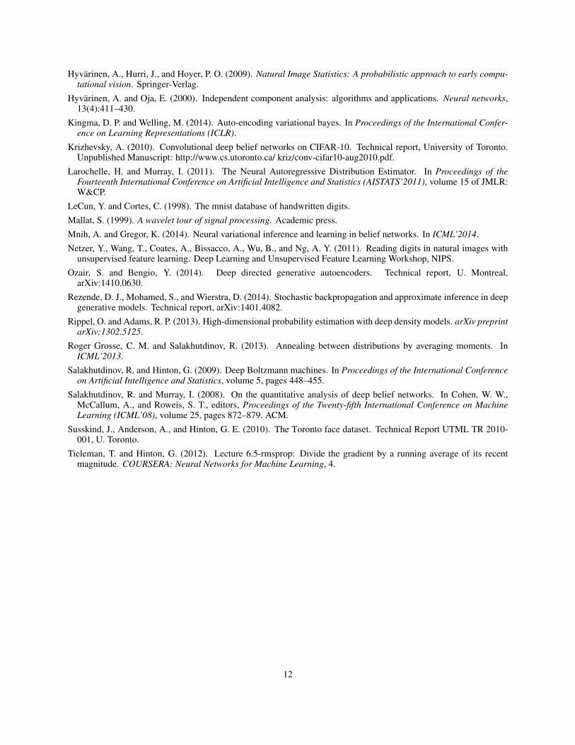
(a) TFD test examples (b) Initial state (c) MAP inference of the state

Figure 7: Inpainting on TFD. The adopted procedure is the same as the one used in MNIST (see caption Fig 6).

10

7 Conclusion

In this work we presented a new flexible architecture for learning a highly non-linear transformation that maps thetraining data to a space where its distribution is approximately factorized, and a framework to achieve this by directlymaximizing log-likelihood. Our model features efficient unbiased ancestral sampling and achieves competitive resultson log-likelihood and inpainting.

Note that the architecture of our model could be trained using other inductive principles capable of exploiting itsadvantages, like toroidal subspace analysis (TSA) (Cohen and Welling, 2014).

We also briefly make a connection with variational autoencoders. Additional work can be made in that direction toallow more powerful approximate inference, with a more complex family of approximate posterior distributions, or aricher family of priors.

Acknowledgements

We would like to thank Yann Dauphin, Vincent Dumoulin, Aaron Courville, Kyle Kastner, Dustin Webb and Li Yaofor discussions and feedback. Vincent Dumoulin provided code for visualization. They are grateful towards thedevelopers of Theano (Bergstra et al., 2011) (Bastien et al., 2012) and Pylearn2 (Goodfellow et al., 2013), and for thecomputational resources provided by Compute Canada and Calcul Quebec, and for the research funding provided byNSERC, CIFAR, and Canada Research Chairs.

ReferencesBastien, F., Lamblin, P., Pascanu, R., Bergstra, J., Goodfellow, I. J., Bergeron, A., Bouchard, N., and Bengio, Y.

(2012). Theano: new features and speed improvements. Deep Learning and Unsupervised Feature Learning NIPS2012 Workshop.

Bengio, Y. (1991). Artificial Neural Networks and their Application to Sequence Recognition. PhD thesis, McGillUniversity, (Computer Science), Montreal, Canada.

Bengio, Y. (2009). Learning deep architectures for AI. Now Publishers.

Bengio, Y. (2014). How auto-encoders could provide credit assignment in deep networks via target propagation.Technical report, arXiv preprint arXiv:1407.7906.

Bengio, Y. and Bengio, S. (2000). Modeling high-dimensional discrete data with multi-layer neural networks. InSolla, S., Leen, T., and Muller, K.-R., editors, Advances in Neural Information Processing Systems 12 (NIPS’99),pages 400–406. MIT Press.

Bengio, Y., Mesnil, G., Dauphin, Y., and Rifai, S. (2013). Better mixing via deep representations. In Proceedings ofthe 30th International Conference on Machine Learning (ICML’13). ACM.

Bergstra, J., Bastien, F., Breuleux, O., Lamblin, P., Pascanu, R., Delalleau, O., Desjardins, G., Warde-Farley, D.,Goodfellow, I. J., Bergeron, A., and Bengio, Y. (2011). Theano: Deep learning on gpus with python. In Big Learnworkshop, NIPS’11.

Bishop, C. M. (2006). Pattern Recognition and Machine Learning. Springer.

Cohen, T. and Welling, M. (2014). Learning the irreducible representations of commutative lie groups. arXiv preprintarXiv:1402.4437.

Goodfellow, I. J., Pouget-Abadie, J., Mirza, M., Xu, B., Warde-Farley, D., Ozair, S., Courville, A., and Bengio, Y.(2014). Generative adversarial networks. Technical Report arXiv:1406.2661, arxiv.

Goodfellow, I. J., Warde-Farley, D., Lamblin, P., Dumoulin, V., Mirza, M., Pascanu, R., Bergstra, J., Bastien, F., andBengio, Y. (2013). Pylearn2: a machine learning research library. arXiv preprint arXiv:1308.4214.

Gregor, K., Danihelka, I., Mnih, A., Blundell, C., and Wierstra, D. (2014). Deep autoregressive networks. InICML’2014.

11

Hyvarinen, A., Hurri, J., and Hoyer, P. O. (2009). Natural Image Statistics: A probabilistic approach to early compu-tational vision. Springer-Verlag.

Hyvarinen, A. and Oja, E. (2000). Independent component analysis: algorithms and applications. Neural networks,13(4):411–430.

Kingma, D. P. and Welling, M. (2014). Auto-encoding variational bayes. In Proceedings of the International Confer-ence on Learning Representations (ICLR).

Krizhevsky, A. (2010). Convolutional deep belief networks on CIFAR-10. Technical report, University of Toronto.Unpublished Manuscript: http://www.cs.utoronto.ca/ kriz/conv-cifar10-aug2010.pdf.

Larochelle, H. and Murray, I. (2011). The Neural Autoregressive Distribution Estimator. In Proceedings of theFourteenth International Conference on Artificial Intelligence and Statistics (AISTATS’2011), volume 15 of JMLR:W&CP.

LeCun, Y. and Cortes, C. (1998). The mnist database of handwritten digits.Mallat, S. (1999). A wavelet tour of signal processing. Academic press.Mnih, A. and Gregor, K. (2014). Neural variational inference and learning in belief networks. In ICML’2014.Netzer, Y., Wang, T., Coates, A., Bissacco, A., Wu, B., and Ng, A. Y. (2011). Reading digits in natural images with

unsupervised feature learning. Deep Learning and Unsupervised Feature Learning Workshop, NIPS.Ozair, S. and Bengio, Y. (2014). Deep directed generative autoencoders. Technical report, U. Montreal,

arXiv:1410.0630.Rezende, D. J., Mohamed, S., and Wierstra, D. (2014). Stochastic backpropagation and approximate inference in deep

generative models. Technical report, arXiv:1401.4082.Rippel, O. and Adams, R. P. (2013). High-dimensional probability estimation with deep density models. arXiv preprint

arXiv:1302.5125.Roger Grosse, C. M. and Salakhutdinov, R. (2013). Annealing between distributions by averaging moments. In

ICML’2013.Salakhutdinov, R. and Hinton, G. (2009). Deep Boltzmann machines. In Proceedings of the International Conference

on Artificial Intelligence and Statistics, volume 5, pages 448–455.Salakhutdinov, R. and Murray, I. (2008). On the quantitative analysis of deep belief networks. In Cohen, W. W.,

McCallum, A., and Roweis, S. T., editors, Proceedings of the Twenty-fifth International Conference on MachineLearning (ICML’08), volume 25, pages 872–879. ACM.

Susskind, J., Anderson, A., and Hinton, G. E. (2010). The Toronto face dataset. Technical Report UTML TR 2010-001, U. Toronto.

Tieleman, T. and Hinton, G. (2012). Lecture 6.5-rmsprop: Divide the gradient by a running average of its recentmagnitude. COURSERA: Neural Networks for Machine Learning, 4.

12