Embed Size (px)
Citation preview

Newsletter
New methodology to better understand fatigue life in complex components
The Simulation Based Engineering & Sciences Magazine
Development of a methodology and tools for tolerances in vehicle electrification to meet future customer demand and ensure competitive advantage
Creating an accurate digital twin of a human user forrealistic modeling and simulation
Initial usage data of new Web app
created to facilitate design of planing hulls
Initial usage data of new Web app
created to facilitate design of planing hulls
Year 16 n°1
Spring 2019

Newsletter - Spring 2019 3
Digital Transformation is becoming the buzzword of 2019, with companies from all sectors investing time, effort and money to embrace this important
phase of the move to Industry 4.0. In fact, the recently published International Data Corporation (IDC) Worldwide Semiannual Digital Transformation Spending Guide expects worldwide spending on the enabling technologies and services related to the digital transformation of business practices, products and organizations to reach $1.97 trillion in 2022, representing a compound annual growth rate of 16.7% from 2017 to 2022. The discrete manufacturing, process manufacturing, transportation and retail sectors are expected to account for almost half the spend in 2019, with the top priority for the two manufacturing sectors being smart manufacturing, followed by digital innovation and digital supply chain optimization, according to IDC. IDC reports the important projects across all sectors to be freight management, autonomic operations, robotic manufacturing and intelligent and predictive grid management for electricity, gas and water. The report states that Europe is the third largest geography for digital transformation spending, after the United States and China.IDC’s report finds the European manufacturing sector to be focusing on the adoption of innovation accelerator technologies for production processes, asset and inventory management, and new sales models based on IoT, robotization, artificial intelligence, machine learning and 3D printing. For those of us in the Simulation-based Engineering and Sciences sector, it is increasingly important to critically examine all the aspects of the digital transformation trend
and our actual and potential roles in it, to pre-emptively identify the emerging and potential
business and technology opportunities inherent in it.
With the pace of change accelerating exponentially, industry events like the International CAE Conference and Exhibition, now in its 35th year, allow stakeholders to dive deeply into the technologies, trends and thinking shaping our world. The 2019 International CAE Conference and Exhibition will provide an important occasion to industry players – both users and purveyors – to take stock of the digital transformation trend, identify the opportunities and challenges being created, and discuss the possibilities with opinion leaders and peers. The new Exhibition space particularly promises to showcase many interesting and emerging aspects of this trend, making it even more critical to participate as exhibitors and attendees. Bookings for exhibition space are already open and interest is avid (contact the organizers at [email protected] for more information).To be serious contenders in the Industry 4.0 landscape, and to continue to offer significant competitive advantage en route, we players in SBES must reflect on the trends now, identify the opportunities to add value and to innovate, take stock of the challenges to be overcome, and then apply our ingenuity and significant problem-solving capacities to help our customers adapt so that we, too, can thrive. This issue of the Newsletter is once again full of case studies and examples of such ingenuity and problem-solving ability. These are fundamental qualities that the SBES community must harness and collectively apply to this emerging world, to shape it into something that enhances the long-term security and wellbeing of all by participating responsibly in resolving our contribution to the critical problems of the planet in terms of climate change and sustainable development.
Stefano Odorizzi, Editor in chief
Flash
CALL FOR PAPERS
Vicenza, ITALYVicenza Convention Centre @Fiera di Vicenza
2019, 28 - 29 OCTOBER
www.caeconference.com
35th INTERNATIONALCAE CONFERENCE AND EXHIBITION
HOW TO SUBMIT YOUR ABSTRACT
Abstracts must be submitted using the online abstract submission form in the
etisbew eht fo aera ecnerefnoC (www.caeconference.com)
ABSTRACT SUBMISSION DEADLINE
2019, 21st June
ACCEPTANCE NOTIFICATION 2019, 9th July
FINAL PAPER SUBMISSION DEADLINE
2019, 23rd September
For more information: [email protected]
Phone +39 342 6496272
EDITOR’S NOTE

Newsletter - Spring 2019 54 Newsletter - Spring 2019
CONTENTSCONTENTS
Newsletter EnginSoftYear 16 n°1 - Spring 2019To receive a free copy of the next EnginSoft Newsletters, please contact our Marketing office at: [email protected]
All pictures are protected by copyright. Any reproduction of these pictures in any media and by any means is forbidden unless written authorization by EnginSoft has been obtained beforehand. ©Copyright EnginSoft Newsletter.
EnginSoft S.p.A.24126 BERGAMO c/o Parco Scientifico TecnologicoKilometro Rosso - Edificio A1, Via Stezzano 87Tel. +39 035 368711 • Fax +39 0461 97921550127 FIRENZE Via Panciatichi, 40Tel. +39 055 4376113 • Fax +39 0461 97921635129 PADOVA Via Giambellino, 7Tel. +39 049 7705311 • Fax +39 0461 97921772023 MESAGNE (BRINDISI) Via A. Murri, 2 - Z.I.Tel. +39 0831 730194 • Fax +39 0461 97922438123 TRENTO fraz. Mattarello - Via della Stazione, 27Tel. +39 0461 915391 • Fax +39 0461 97920110133 TORINO Corso Marconi, 10Tel. +39 011 6525211 • Fax +39 0461 979218
www.enginsoft.come-mail: [email protected]
The EnginSoft Newsletter is a quarterly magazine published by EnginSoft SpA
COMPANY INTERESTSEnginSoft GmbH - GermanyEnginSoft UK - United KingdomEnginSoft France - FranceEnginSoft Nordic - SwedenEnginSoft Turkey - TurkeyVSA-TTC3 - Germanywww.enginsoft.com
CONSORZIO TCN www.consorziotcn.it • www.improve.itSimNumerica www.simnumerica.itM3E Mathematical Methods and Models for Engineering www.m3eweb.it
ASSOCIATION INTERESTSNAFEMS International www.nafems.it • www.nafems.orgTechNet Alliance www.technet-alliance.com
ADVERTISING For advertising opportunities, please contact our Marketing office at: [email protected]
RESPONSIBLE DIRECTORStefano Odorizzi
PRINTING Grafiche Dalpiaz - Trento
Autorizzazione del Tribunale di Trento n° 1353 RS di data 2/4/2008
The EnginSoft Newsletter editions contain references to the following products which are trademarks or registered trademarks of their respective owners: ANSYS, ANSYS Workbench, AUTODYN, CFX, FLUENT, FORTE’, SpaceClaim and any and all ANSYS, Inc. brand, product, service and feature names, logos and slogans are registered trademarks or trademarks of ANSYS, Inc. or its subsidiaries in the United States or other countries. [ICEM CFD is a trademark used by ANSYS, Inc. under license]. (www.ANSYS.com) - modeFRONTIER is a trademark of ESTECO Spa (www.esteco.com) - Flownex is a registered trademark of M-Tech Industrial - South Africa (www.flownex.com) - MAGMASOFT is a trademark of MAGMA GmbH (www.magmasoft.de) - FORGE, COLDFORM and FORGE Nxt are trademarks of Transvalor S.A. (www.transvalor.com) - LS-DYNA is a trademark of LSTC (www.lstc.com) - Cetol 6s is a trademark of Sigmetrix L.L.C. (www.sigmetrix.com) - RecurDyn™ and MBD for ANSYS is a registered trademark of FunctionBay, Inc. (www.functionbay.org) Maplesoft are trademarks of MaplesoftTM, a subsidiary of Cybernet Systems Co. Ltd. in Japan (www.maplesoft.com) - Particleworks is a trademark of Prometech Software, Inc. (www.prometechsoftware).
Contents6 Soft skills, sound methodology and statistical analysis
will be key to successful industry 4.0 implementations
8 New methodology to better understand fatigue life in complex components
by Emak and EnginSoft
Case Studies
17 Takenaka Corporation automates simulation-based architectural design
by Takenaka and Esteco
18 Improving the performance of shaped charges and passive ballistic protections
by Rina Consulting
22 Development of a methodology and tools for tolerances in vehicle electrification to meet future customer demand and ensure competitive advantage
by EnginSoft and Metasystem
24 Initial usage data of new Web app created to facilitate design of planing hulls
by CINECA
27 Multi-purpose ANSYS APDL script developed for analysis of matter-radiation interaction
by INFN and Sapienza University of Rome
32 Creating an accurate digital twin of a human user for realistic modeling and simulation
by Biomotion Solutions
36 CivilFEM enables interaction analysis between structures and geotechnics
by Ingeciber
39 New approach for accurate, robust morphing of CAD geometries
by International TechneGroup
44 Optimizing a cam mechanism using Adam and MATLAB
by Sidel GROUP and EnginSoft
46 Numerical Computation Technique to Examine Glass Fiber Mat and Cloth Reinforcement of Glass-Fiber-Reinforced Plastic
by TDK Corporation
52 Tribology solutions for fluid lubricated bearings in machines
by AIES
56 How to reduce fatigue analysis calculation times with ANSYS nCode DesignLife
58 MAGMASOFT releases version 5.4
60 Prometech Software releases Particleworks 6.2 and Granuleworks 1.1
62 FunctionBay announces the release of RecurDyn V9R2
64 New, extended capabilities of PASS/Nozzle-FEM
68 Total Materia updated with two new modules
69 Numerical simulation thesis on road safety wins Lorenzo Argenti Degree Award
70 Report back from 2018 Prometech Simulation Conference and GPU Computing Workshop in Japan
Software Updates
Press Releases
Interview
PAST ISSUES atwww.enginsoft.com/magazine

Newsletter - Spring 2019 76 Newsletter - Spring 2019
INTERVIEWINTERVIEW
Which technician is best suited to work on this? A good mathematical background and solid experience in computer vision is important but, the applications today are VERY different from what they were. So, by methodology I mean being able to manipulate general or symbolic concepts or building blocks and assemble them in a different way. Our engineers from Italian universities are very good at that.Team work is a very important soft skill and represents a challenge, even in the academic environment. Most interesting industrial problems are multidisciplinary and it’s difficult to get different professors working together. You find mechanical engineers, for example, are most comfortable working with other mechanical engineers. Instead, there is great value in having a rainbow of competences. There are big differences in approach between an engineer and a mathematician, so everyone can learn from one another, provided they have the maturity to engage competently. This is difficult to achieve and takes time to develop.Continuous leaning is mandatory for everyone today. Firstly, it is an investment in yourself, because it improves your attractiveness to the labor market. Secondly, it helps you avoid the risk of missing opportunities. People must be willing to constantly train, to try, and to learn. These and other soft skills are already being seen to be the real value for a company. When comparing Italy to the USA, for example, I see an evident gap between the required competences and the possessed competences, possibly because staff turnover is so high in the US, even within the same company, that it’s difficult for people to acquire the necessary technical competence. As a result, US companies need to define everything in great detail in terms of procedures. On the contrary, in Italy there is a more independent approach: everyone can confront a problem, define it and solve it. But every company has a limited ability to offer eternal evolution to its staff. Some companies, such as mine, do offer continuous opportunities to collaborate with the research market and to constantly innovate. This is important, but not all companies have this culture. So, another valuable place to find learning opportunities is through ongoing contact with suppliers and customers. It provides incredible opportunities to see the market with new eyes, to view the other products, solutions, companies or networks available on the market. The Internet is a further incredible opportunity to discover the tip of the iceberg in new areas, after which knowledge can be deepened more formally.
Q. Are there other specific challenges to Industry 4.0 that you see in Italy?A. Today, only the large companies are ready – or almost ready – to speak about Industry 4.0. On the other hand, it’s almost impossible for small- or medium-sized companies to embrace all the possibilities in the short term. 25,000 SMEs polled in Italy have an average of seven employees. This means Italian companies are very limited in terms of time, and the economic and human resources to approach Industry 4.0 in a structured way. Italian companies are smart enough to offer very tailored solutions, but they not big enough to offer comprehensive solutions. This is very limiting. There are only a few Italian companies that are big enough to embrace Industry 4.0 technology and then sell it on. Adige is one of these. But we are also small when compared to a German or Chinese company. We are big in Italy, but we are small enough to be fast in adopting these solutions.
Q. You mentioned that one of the pitfalls of Industry 4.0 is chasing technology for technology’s sake. Are there any others to be aware of?A. The key objective of Industry 4.0 is to improve the way we do our jobs, to do them better. One of the most attractive possibilities of Industry 4.0 is that every single piece of electronics, mechanics or software can potentially collect information and transfer it to the cloud, giving us all this raw data. Potentially, using artificial intelligence, a data mining algorithm, or some form of machine learning, you can then dig into this data to find patterns, regularities or irregularities among the confusion, even if you don’t know what you’re looking for. This is the ideal that is being advertised everywhere. I agree that discovering biases in the data could be reasonable in some cases, such as in very mechanical processes that are always the same for weeks or months. But it’s very different if a production or manufacturing process is flexible: we sell a machine that does different things each day. What is the relationship between the huge amount of data I collect from the sensors in this type of machine? No-one knows, but everyone is fascinated, and so we are all collecting huge amounts of data.We cannot, and must not, however, become lovers of data for data’s sake. Instead, we need to select the data that we need, get it into the hands of the people to analyze it and then we need to apply the findings. We need to become better at discarding unnecessary data and be open to changing what data we collect. The challenge is to discover what is really important. The answer is that only a small fraction will be important. At a major fair in Hanover for laser technology just recently, everyone was saying “we collect data”, but no-one was saying how to draw the knowledge from the data. The cautious attitude is to say, there is some information I would like to know and statistically analyze today, and then there is potentially much more data, but it is practically useless at the moment. Incidentally, this has created a whole new area for statistical analysis. As a result, there has been an increase in interest in statistics and math graduates to dig some kind of order out of all this data chaos. Currently, as a manager, I would be happy to have a summary of the overall behavior of our systems – half a page of statistics, no more. The technicians on the floor will probably need and want more.
Q. What do you believe the most important priority should be now for companies in considering Industry 4.0?A. Most engineering companies and consultants are pushing the exploitation and application of simulation to improve products or systems. Instead, I think that the bigger short-term benefit can be had from improving the logistics between systems – the flow of information and materials. This is something that we truly battle with every day. Most of the inefficiencies I see currently come from inefficient logistics. My customers also confirm this. Everyone is looking at their systems as islands, when they should be viewed as a network from supplier to producer to final customer. No-one is really skilled in this and it is the missing link. We need an approach that is more systemic. So, we come back to what I was saying earlier when I was talking about methodology. Realistic simulation is important; digital twins etc. are all important: you can get processes to be faster and more economical, but in the end, you can achieve a greater benefit by becoming more efficient between one part of the process and the next.
Soft skills, sound methodology and statistical analysis will be key to successful industry 4.0 implementationsPaolo Benatti, Technical Director of Adige in the BLM Group, was one of the panel members in the Industry 4.0 Round Table session at the International CAE Conference in Vicenza from 8-9 October. In this interview he explains the challenges to be overcome for Industry 4.0 and the competences that will be required of companies and their staff.
Q. What are some of the obstacles you see in the move to Industry 4.0 in Italy?A. One of the greatest fears is that robotics will substitute human beings, reducing employment by industry. I disagree. A lot of articles on this subject from different perspectives instead suggest that there will be a switch in the types of competences required by industry: we will need more skilled engineers and less pure manpower on the floor, but the total amount of employment will remain the same. The requirement for problem-solving capabilities will increase substantially. At Adige, our technical department already spends time daily on the production floor, side by side with the technicians in the production line, as well as in training courses. This is important because we offer very deep integration between our production facility and the production-flow logic, which requires us to meet with every customer to discuss their needs, which are similar but different. To meet their needs, we have to understand their requirements and transform them into solutions – a challenge that is 50% mechatronics and 50% human problem solving.
A changing world requires people that cope with change. We face an industrial future where industrial suppliers will no longer sell closed machines but rather machines biased towards services. This will require your staff to develop different skills than those they have today. Retaining your approaches, methodologies and your people remains fundamental, however.A further requirement will be for management and staff to become open-minded about company structures and processes, and with customers and suppliers. Industry 4.0 imposes a rapid rate of change on production approaches in general, as well as on the entire work process, which requires mental flexibility. These competences are not developed only by studying formally, but by frequently changing the problems and challenges that you face daily. For instance, digital twins are a “hot topic”
of Industry 4.0 but they require very wide and deep competence in the models being discussed – even if those models are logistics. There are very few people competent to do this from day to day and remain fresh in their approach, looking at the model in a new way, as a new problem. Yet, the mental flexibility of our youngest engineers needs to be paired with the skills and experience of the old technical engineers in your company to exploit the valuable experience dynamically without ignoring the benefits offered by technology. Furthermore, technology transfer is important because ICTs can be applied to industrial problems with limited thought. So, enthusiasm is a highly valuable quality, but it needs to be balanced with sound experience. This is also important to avoid becoming too distracted by technology and losing sight of the concrete benefits.
As a final point, in its current phase, industry 4.0 is like a video game: many people are wasting time chasing potential solutions that are not real yet. Every day, I see new technologies, new kinematics, new motors, new software that could be applied successfully in our business, but I’m not knowledgeable enough to see where or how to best to exploit them. Not all companies have the capacity to invest the time in understanding if a technology is applicable and where its advantage lies, which requires attention and team work. So, we need to be very cautious and prudent because only a tiny fraction of all these new technologies are likely to become important in the long term.
Q. What new competences will employees require?A. As I’ve already mentioned, methodology or approach is more important than specific knowledge because it’s almost impossible to know what competences will be required tomorrow. But the time frames are very fast -- in the order of months not years. Curiosity and mental flexibility are important, but the safest competences to acquire are a methodological approach and soft skills. With a strong math and physics or engineering background and a good methodology, you will be able to do anything. If you are too specialized, you can be good today, but tomorrow – I don’t know. Real innovation today lies in creatively transferring or applying what already exists to new areas. With materials, for instance, innovation lies in applying or exploiting an existing material differently. Another example is computer vision. In the automotive industry, it allows cars to follow the road, or assists drivers with parking guidance. The technology cost today is very low, but the potential of the solution is enormous.

Newsletter - Spring 2019 98 Newsletter - Spring 2019
CASE STUDIES CASE STUDIES
An important cause of failure in machines with complex components is fatigue from vibration due to being subject to multiple forces that vary over time. While these machines undergo extensive testing both at the bench and in the field, engineers need a generalized methodology to better calculate the fatigue in the presence of any number of known loads in time for a given cycle, in order to improve the estimation of the components’ fatigue life and effectively integrate that into the product development process. This technical article details the application of the methodology developed using ANSYS WorkBench.
New methodology to better understand fatigue life in complex components First six months’ use demonstrates comprehensive usability for designers with open future development prospects
By Paolo Verziagi1, Valentina Peselli2 and Daniele Calsolaro2
1. EMAK - 2. EnginSoft
EMAK produces machines for gardening, agriculture and civil construction. The company develops its two-stroke engines for hand-held use like chainsaws, brushcutters, blowers, etc. One of the main causes of failure is fatigue from vibration, so engineers need a methodology to better understand what happens in a durability/field test. The aim of this paper is to explain the strategy adopted to estimate the life of the components in a professional brushcutter using ANSYS Workbench, one of the most popular brands of commercial software. It was a challenging undertaking because it requires interdisciplinary knowledge covering signal processing, fatigue, vibration mechanics, loss factor estimation, Fixed Element Analysis (FEA), IT, etc.
General information about the procedureThe fatigue calculation of components is essential whenever a part or assembly is subject to repeated forces over time, whatever their nature. In this context, we are talking about the forces generated by the dynamics of the 2T motor and the forces deriving from the tool-side load; forces that involve a dynamic response from the structure itself. The evaluation of the fatigue life of such complex components,
subject to multiple forces that vary over time, is neither simple nor immediate and therefore must be effectively integrated into the product development process (Fig.1).
Numerical procedureThere are four initial assumptions that are fundamental to subsequent evaluations when conducting a fatigue life analysis:
1) The quantification of the variable loads in time Fk(t) that the moving parts of the machine and the possible presence of the tool could unload onto the structure. In this regard, it is useful to set up a “multi-body” analysis, with rigid or rigid-flexible bodies, to represent the kinematics of the machine’s operation.
2) Analysis of the signal over time and the identification of the best strategy to reproduce the physical phenomenon from the computational point of view. Since the machine is subject to a predefined cycle that is repeated in time, and since we are interested in the phase of the behavior regime which allows us to overlook the initial transient phase, a possible
strategy is to move from the time domain to the frequency domain by solving a series of harmonic analyses, obviously working within the hypothesis that the system behaves linearly for the entity of the vibrations in play.
3) The generation, running and validation of the dynamic Finite Element (FE) model of the machine. The FE model, with the appropriate material properties in terms not only of stiffness and inertia, but also of intrinsic damping, once realized and solved, must be experimentally validated; this can be achieved by correlating the numerical frequency responses with the experimental ones. The activity is then set up on machines that already have physical test samples, to allow the calibration of any unknown parameters (such as friction-related damping, for example) and their subsequent validation. Once calibrated and validated, the procedure can be used on new machines of the same type.
4) Learning the fatigue behavior of the material. The material fatigue curves must be accurately acquired as they have a decisive influence on the results obtained. The ideal, of course, would be to proceed with experimental tests, material by material, to acquire the curves of every specific sample extracted from each component, which would then also record the specific production processes. In the absence of specific real curves, one can use bibliographic data which while certainly faster and cheaper, leaves a level of uncertainty about the actual behavior of the product.
For this specific case, the procedure developed was set up and applied to a professional brushcutter with a displacement of over 50cc. Below we have analyzed the main stages of setting up the procedure.
Step 1: Quantification of time-varying loads Fk, Multi-body modelIn the multibody simulation, we modelled the crank thrust and the combustion signal of the power unit (PU), the behavior of the clutch (which decouples the transmission below approximately 4000rpm), the bevel gear that multiplies the engine torque and the cutting device (UT). In particular, the drive shafts were made flexible to account for the different binding reactions discharged onto the bearing
Fig. 1 - Calculation of fatigue life within the product development process.
Fig. 2 - MAPLESIM model with the concentrated parameters of the 50cc professional brushcutter.
CASE STUDIES
Newsletter - Spring 2019 1110 Newsletter - Spring 2019
CASE STUDIES CASE STUDIES
Since the procedure is completely parametric, it is important to include all the areas for which you will subsequently study the fatigue life in the appropriate named selection, to be able to replicate the methodology on new geometries using the same approach. This aspect is equally indispensable to reduce the file size of the results produced by limiting the saved results only to the areas of interest.
Thermal analysisDuring operation, the average temperature of the various parts of the machine is not the ambient temperature, instead it tends to settle at a constant value that varies from point to point after a few minutes of operation; this is especially true in bench tests where the cycle is repeated over many hours: once fully operational, the fluctuations in temperature over time are minimal. For this reason, in order to make the following evaluations, one cannot ignore a thermal pre-stress analysis to introduce the average stress condition to which the machine is subjected, nor if you have the S-N curves available when the temperature varies, to choose the appropriate curve to use, point by point. The average stress that results from this will be important to correct the fatigue resistance and therefore to reconstruct the time history of the equivalent voltage of a given node. Thanks to previous experience with the fluid dynamics of PU cooling, we know the thermal powers, the heat exchange coefficients and the temperatures, which allows us to reconstruct a thermal field that qualitatively represents the real temperature map of the system during operation by running an FE simulation.
Static analysisTo calculate the average pre-stress condition to which the system is subject, it is necessary to conduct a static simulation that contains all the “static” average loads present in the system being examined.Besides the temperature conditions calculated by means of the thermal analysis, and the possible average contributions of the variable loads in time obtained from the multibody simulation, the pretension bolts that keep together the various parts of the whole play an important role in the calculation of the pre-stress to which the machine is subjected; the screws and their surroundings are generally meshed by finely controlling the dimensions of the element, to better capture certain gradients of tension and to accurately evaluate the effective clamping area (through appropriate frictional contacts that will become bonded only in the areas of effective contact in the next frequency sweep). Regarding the constraints assigned to the structure, zero displacements and rotations were imposed on the
centroid of the handlebar’s extremity and at the attachment point of the belt. It should be noted that the handlebars and the shaft of Fig. 2 are connected to the rest of the machine by means of four spring-loaded vibration dampers shaped like linear bushings with adequate stiffness and damping values derived from careful static and dynamic characterizations.The average values of the 19 force components within the duty cycle discussed above were assigned as forces on the nodes and oriented according to a nodal reference system. In pre-stress statics, gravity is also considered, which by itself entails a certain deformation of the entire structure given the not insignificant weight of the brushcutter during operation (about 10 kg). The results file of this static analysis of the average pre-stress is saved in the file “statica.rst”.
Frequency sweep analysisAfter suitably linearizing the model realized for the different material properties and for the definition of the contacts, we set up a harmonic sweep in the 0-400 Hz range, with a frequency step of 0.1 Hz to
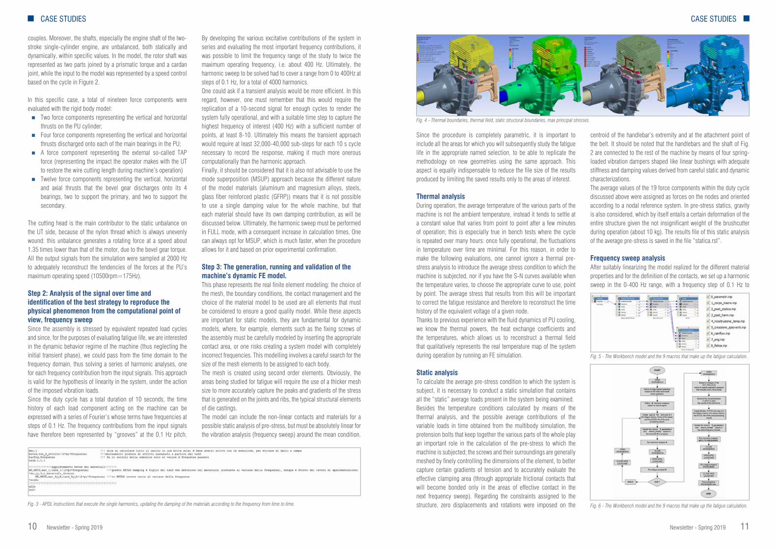
Fig. 4 - Thermal boundaries, thermal field, static structural boundaries, max principal stresses.
Fig. 5 - The Workbench model and the 9 macros that make up the fatigue calculation.
Fig. 6 - The Workbench model and the 9 macros that make up the fatigue calculation.
couples. Moreover, the shafts, especially the engine shaft of the two-stroke single-cylinder engine, are unbalanced, both statically and dynamically, within specific values. In the model, the rotor shaft was represented as two parts joined by a prismatic torque and a cardan joint, while the input to the model was represented by a speed control based on the cycle in Figure 2.
In this specific case, a total of nineteen force components were evaluated with the rigid body model: n Two force components representing the vertical and horizontal
thrusts on the PU cylinder;n Four force components representing the vertical and horizontal
thrusts discharged onto each of the main bearings in the PU;n A force component representing the external so-called TAP
force (representing the impact the operator makes with the UT to restore the wire cutting length during machine’s operation)
n Twelve force components representing the vertical, horizontal and axial thrusts that the bevel gear discharges onto its 4 bearings, two to support the primary, and two to support the secondary.
The cutting head is the main contributor to the static unbalance on the UT side, because of the nylon thread which is always unevenly wound: this unbalance generates a rotating force at a speed about 1.35 times lower than that of the motor, due to the bevel gear torque. All the output signals from the simulation were sampled at 2000 Hz to adequately reconstruct the tendencies of the forces at the PU’s maximum operating speed (10500rpm=175Hz).
Step 2: Analysis of the signal over time and identification of the best strategy to reproduce the physical phenomenon from the computational point of view, frequency sweepSince the assembly is stressed by equivalent repeated load cycles and since, for the purposes of evaluating fatigue life, we are interested in the dynamic behavior regime of the machine (thus neglecting the initial transient phase), we could pass from the time domain to the frequency domain, thus solving a series of harmonic analyses, one for each frequency contribution from the input signals. This approach is valid for the hypothesis of linearity in the system, under the action of the imposed vibration loads.Since the duty cycle has a total duration of 10 seconds, the time history of each load component acting on the machine can be expressed with a series of Fourier’s whose terms have frequencies at steps of 0.1 Hz. The frequency contributions from the input signals have therefore been represented by “grooves” at the 0.1 Hz pitch.
By developing the various excitative contributions of the system in series and evaluating the most important frequency contributions, it was possible to limit the frequency range of the study to twice the maximum operating frequency, i.e. about 400 Hz. Ultimately, the harmonic sweep to be solved had to cover a range from 0 to 400Hz at steps of 0.1 Hz, for a total of 4000 harmonics. One could ask if a transient analysis would be more efficient. In this regard, however, one must remember that this would require the replication of a 10-second signal for enough cycles to render the system fully operational, and with a suitable time step to capture the highest frequency of interest (400 Hz) with a sufficient number of points, at least 8-10. Ultimately this means the transient approach would require at least 32,000-40,000 sub-steps for each 10 s cycle necessary to record the response, making it much more onerous computationally than the harmonic approach.Finally, it should be considered that it is also not advisable to use the mode superposition (MSUP) approach because the different nature of the model materials (aluminum and magnesium alloys, steels, glass fiber reinforced plastic (GFRP)) means that it is not possible to use a single damping value for the whole machine, but that each material should have its own damping contribution, as will be discussed below. Ultimately, the harmonic sweep must be performed in FULL mode, with a consequent increase in calculation times. One can always opt for MSUP, which is much faster, when the procedure allows for it and based on prior experimental confirmation.
Step 3: The generation, running and validation of the machine’s dynamic FE model.This phase represents the real finite element modeling: the choice of the mesh, the boundary conditions, the contact management and the choice of the material model to be used are all elements that must be considered to ensure a good quality model. While these aspects are important for static models, they are fundamental for dynamic models, where, for example, elements such as the fixing screws of the assembly must be carefully modeled by inserting the appropriate contact area, or one risks creating a system model with completely incorrect frequencies. This modelling involves a careful search for the size of the mesh elements to be assigned to each body.The mesh is created using second order elements. Obviously, the areas being studied for fatigue will require the use of a thicker mesh size to more accurately capture the peaks and gradients of the stress that is generated on the joints and ribs, the typical structural elements of die castings. The model can include the non-linear contacts and materials for a possible static analysis of pre-stress, but must be absolutely linear for the vibration analysis (frequency sweep) around the mean condition.
Fig. 3 - APDL instructions that execute the single harmonics, updating the damping of the materials according to the frequency from time to time.
Newsletter - Spring 2019 1312 Newsletter - Spring 2019
CASE STUDIES CASE STUDIES
system’s response to the loads applied as input. In particular, this macro reads the file of the harmonic results for the various frequencies analyzed, first loading the real part and then the imaginary part for each of them. An array called “post_harm_nodeXXX”, which consists of as many rows as the harmonics analyzed and 16 columns with the real and imaginary parts of all the voltage tensor components, and the equivalent von Mises voltage, is generated for each node of interest. For example, for the node 92899 you get the following “post_harm_node92899” array:
Macro “4_reconstruction_temp.inp”.This corresponds to the reconstruction of the temporal response of the signed von Mises voltage for the temporal duration of the load cycle on the nodes of interest. This reconstruction is based on the results of the prestress static analysis and of the harmonic analysis generated and post-processed in the previous steps. In particular, the macro reconstructs all the tensors of the voltages x, y, z, xy, xz, yz for each node and for each temporal step at each instant, and recombines linearly the constant contribution of the statics and the variable contributions in time of the different harmonics, each with its own module, phase and frequency (or equivalently, the real part,
the imaginary part and the frequency). Once the voltage tensor has been reconstructed on each node and for each instant, the equivalent von Mises voltage and the main voltages at that given instant can be calculated. In particular, the Von Mises voltage is calculated with to the following formula where the tensor components are known:
While the main voltages are calculated by solving the following third-degree polynomial for each instant:
Depending on which is the main voltage with higher module, the sign is assigned to the Von Mises previously calculated, thus obtaining
the signed Von Mises (positive if mod(σ1) ≥ mod(σ3), negative if mod(σ13) > mod(σ1));An array called “ricostr_temp_nodeXXX” (XXX is the number of the corresponding node in each case) is then generated for each node of interest, which consists of one row for each time step analyzed and 11 columns that report the time reconstruction of the 6 components
of the voltage tensor, the reconstruction of the main voltages s1 and s3 and of the signed Von Mises; for example, for the node 92899 you get the following “ricostr_temp_node92899” array:
By plotting column 11 of the signed Von Mises Voltage as a function of the times of column 2, one obtains the equivalent uniaxial response of the system for that specific node (for example, node 92899) as the time varies, which is useful to evaluate the fatigue life. During this phase, the procedure also evaluates the absolute maximum and minimum values recorded by the time history of the generic node’s signed von Mises and saves them in the variables max_assol_nodeXXX and min_assol_nodeXXX.
Macro “5_creation_spiovents.inp”.This macro simplifies the temporal history of the signed Von Mises for each node, transforming them into a history of “levels”, in other words, moving from an analog signal to a digital one. The number of layers used is a parameter “N_bin_x_rainfl” that can be modified within the macro 0_parameters.inp (the higher this number, the more accurate the reconstruction, but the slower the subsequent creation of the rainflow will be). The absolute minimum-maximum interval of the signed Von Mises voltage of the node being examined is divided
N°NODO freq σx, RE σx, IM σy, RE σy, IM σz, RE σz, IM σxy, RE σxy, IM σxz, RE σxz, IM σyz, RE σyz, RE σeqv, RE σeqv, IM
92899 0.1 1022 -13359 -27381 14821 -602 5188 2412 8342 1361 -7120 -591 17948 29855 158005
… … … … … … … … … … … … … … …
92899 400 6910 31329 960 -11905 -952 -4486 586 3832 946 5338 1753 2521 7968 27048
N°NODO Time σx σy σz σxxy σxz σyz σ1 σ3 σeqv, signed
92899 0 -4.903E6 5.588e5 17.565e6 34.253e6 7.62e6 -3.000e6 18.08e6 -6.7e7 29855
… … … … … … … … … … …
92899 T_fine -53.63e6 -3.59e6 1.34e6 38.15e6 8.20e6 -3.97e6 17.04e6 -7.5e7 -86.015e6
Fig. 8 - Temporal reconstruction of the σeqvVM, signed for node 92899 of the model
cover all the important frequency contributions present, to develop a Fourier series for the temporal histories of the loads to be applied. The corresponding contributions of the series were applied in terms of real and imaginary parts, i.e. module and phase, in the action area of each time-variable load contribution for each frequency. This obviously accounted for any phase delays between the various load conditions. 4000 harmonics were tested in this way.Using the Rayleigh matrix’s definition of appropriate coefficients, the intrinsic damping properties of each material were inserted and varied as the frequency under examination varied, in order to follow the desired trend of tanδ obtained experimentally.
Step 4: Knowledge of material fatigue behaviorThe approach to fatigue proposed in this procedure is STRESS-LIFE or HCF (High Cycle Fatigue). In order to evaluate fatigue life, it is necessary to know the S-N curves for each material under examination. Since the company has never carried out any specific fatigue tests,
the curves referred to were always taken from bibliographic sources of various kinds. The procedure set-up remains valid regardless of the origin of the curves, but obviously the accuracy of the results relies on the validity of the curves chosen. In general, the fatigue curve refers to the specimen tested with an alternating symmetrical load, for example the test performed on the Moore machine; therefore, the curves that must be included in the calculation should consider all the non-ideals that actual pieces offer: much larger dimensions than those of the specimen, radii of curvature and surface finish, higher temperature than the ambient temperature, etc. All this means that the curve must be scaled by a factor, the so-called Kf or strength factor, which according to our experience reaches about 0.4, as shown in Figure 7 (thick green line).
Fatigue analysisThe entire exercise was carried out in the Workbench environment. A suitable set of MAPDL macros which can be launched directly from the Workbench interface using ACT customization, was created for the fatigue procedure. The aim of the activity therefore was the realization of an ANSYS MAPDL procedure for the verification of the fatigue life even of complex assemblies under repetitive load conditions. The
procedure assumes a known test load cycle, thought to be repeated endless times, linked to the bench testing phase of the machine. As a starting point, the procedure requires the resolution of the harmonic analyses considering all the important frequency components necessary to reconstruct the input load cycle, and of the static representing the average conditions. Using the results generated by these simulations, one proceeds to the temporal reconstruction of the voltage history in the points of interest for the temporal duration of the cycle - in particular, one needs to obtain the temporal history of the signed Von Mises. This temporal history is then broken down into a history of peaks and valleys, useful for counting the load cycles using the rainflow procedure. Taking note, therefore, of the load cycles in terms of the mean and alternating voltage and their number present in the temporal history of the signed Von Mises, one then proceeds to correct the alternating voltage taking into account the mean value, according to Soderberg’s theory (one can also insert further criteria to correct the mean value). With these values one enters the S-N curves to calculate each contribution’s number of breaking cycles and therefore the total damage and the fatigue life. A comprehensive explanation of the functionality of each macro is given below.
Macro “0_parameters.inp”.Requires all the parameters useful for the subsequent fatigue analysis to be defined manually by the user. The S-N curves of each material of the components on which you want to perform the fatigue post and the yield stress (useful for correcting the average value of Soderberg) must obviously be included among the various data to be provided.
Macro “1_body_macro.inp”This is the mother macro that calls all the other macros, including the 0_parameters.inp macro, in the right logical order. This is the macro launched by the ACT customization once the parameters have been set in the 0_parameters.inp macro.
Macro “2_post_statica.inp”.This represents the first action to be performed in logical order. It corresponds to the post-processing on the nodes of interest of the static analysis that represents the constant as the time of the system’s response to the loads applied as input varies. In particular, an array called “post_static_nodeXXX” (XXX is the number of the corresponding node in each case) is generated for each node of interest, and consists of a single row with 12 columns that report all the voltage tensor components, the main voltages, and the equivalent von Mises and signed Von Mises voltages. For example, for the node 92899 (a generic node of the conveyor skin) one obtains the following “post_static_node92899” array:
Macro “3_post_harm.inp”.This corresponds to the post-processing on the nodes of interest of the harmonic analyses generated. These represent the variable of the
Fig. 7 - Corrections for different Kf of SN curves for alloy A356.
N°NODE σx σx σz σxy σxx σyz σeqv σ1 σ2 σ3 σeqv_signed
92899 -47859277 -564208 1902138 34498075 7445069 -3354453 78293986 17630100 2849334 -67000783 -78293986

Newsletter - Spring 2019 1514 Newsletter - Spring 2019
CASE STUDIES CASE STUDIES
Macro “7_png.inp”.This macro serves the main macros previously described and is used to generate an external .png image of what was actually plotted.
Macro “8_fatica.inp”.This macro carries out the real fatigue analysis for each node of interest, taking into account the material properties of the component to which it belongs (yield stress value, to correct the mean value, and the S-N curve for the fatigue life). Firstly, it evaluates the correct alternating voltage of the mean value for each half-cycle present in the signed Von Mises temporal history for each node of interest. In fact, column 8 of the spioventi_nodeXXX array shows the value of the
equivalent alternating voltage, obtained after correcting the alternating voltage with respect to the average recorded voltage. The correction was made according to Soderberg’s theory (as requested by the customer):
According to this theory, the correction is applied only if the average voltage is tensile, while no correction is applied in compression. If the average voltage is in modulus greater than the yield strength, however, whether in tension or compression, an infinite alternating voltage is assumed (the macro imposes this equal to 1012 Pa).
Using this equivalent value of alternating voltage, we can enter the corresponding S-N curve (defined for each component of interest in the 0_parameters.inp macro) and calculate the corresponding number of breaking cycles. At the intermediate points of the curve, the value of N for the desired equivalent alternating voltage is interpolated linearly. For voltage values beyond the extremes defined in the curve, N maintains constant the last defined value. This value of N is shown in column 9 of the spioventi_nodeXXX array. In column 10 of this array, we report the damage relative to the semi-cycle considered, which is evaluated as: Damage=0.5/N_cicli_a_rottura; at this point, we are able to evaluate the total breakage damage caused by the signed Von Mises time history for each node, broken down into semi-cycles. To do this we use the Palmgreen-Miner linear damage accumulation rule:
Therefore, adding together all the damage of each semi-cycle for each node studied (reported in column 10 of the spioventi_nodeXXX array), the fatigue damage relative to the load cycle analyzed and thought to be endlessly repeated is obtained. This Damage value for each node is saved in an array called out_fatica_pelle_kkk (where kkk is the index that runs the various defined named_selection on which the fatigue analysis is to be performed). This array has one row for each node making up the named_selection number kkk and 4 columns.
Column 1 shows the number of the node in question, column 2 shows the total damage relative to the entire input time history calculated as described above. Column 3 reports the number of blocks of this load history to reach breakage, calculated as: N_blocchi_arottura=1/Danno_tot; column 4 shows the final fatigue life in hours, calculated as: Vita_ore=N_blocchi_arottura*t_fin*1/3600 dove t_fin is the time duration of the input load cycle. The macro also automatically saves multiple png images that represent the damage map, the number of breaking load blocks and the fatigue life in hours. The out_fatica_pelle_kkk arrays are automatically saved in the workbook in appropriate text files called out_fatica_pelle_kkk.dat (one file for each named_selection), as are the damage and fatigue life maps plotted on the model.
Model validation and resultsThe validation of the model essentially involved two aspects: the first was to ensure that the model of the combustion signal was consistent with the experimental findings, the second was to ensure the best possible correlation between the numerical and the experimental dynamic response (using an instrumented hammer). In examining the transfer function obtained, Figures 14 and 15 show the good degree of correlation achieved, which further reinforces the work done so far.
The same procedure was tested on three different geometries of the same component, called the conveyor, which joins the PU to the brushcutter’s transmission tube, and which had shown some breakages; more precisely:n Geometry01 bench breakage around 200h, breakage in the field
within 10h;n Geometry02 no breakage at the end of the durability bench test
(300h), field breakage between 20 and 50h;n Geometry03 no data available.
In the bench tests, the only excitement that could not be reproduced was the TAP, or the impulsive force due to repeated crushing of the cutting organ; this force was modelled, on the FEM side, as a square impulsive wave of 1600N amplitude and 20ms length, with values deduced from some experimental measurements. The following considerations can be made:
A. There is an excellent correlation around the positioning of the most critical points in terms of fatigue, both for geometry01 and
Fig. 12 - Principles of linear damage accumulation.
Fig. 13 - An example of the out_fatica_pelle_kkkk file.
into N_bin_x_rainfl levels, each with an amplitude equal to abs(max_assol_nodeXXX-min_assol_nodeXXX) / (N_bin_x_rainfl-1). The central value of the level’s voltage is assigned at each level. Level 1 corresponds to the absolute minimum of the signed Von Mises for that node, level N_bin_x_rainfl (for example equal to 50) corresponds to the absolute maximum of the signed Von Mises.
We record the level to which each voltage value of the temporal history of the node being examined corresponds in the first column of the array st_temp_liv_nodeXXX (an array with one row for each temporal step and 2 columns), which therefore represents the rewriting of the temporal history of the signed Von Mises in terms of a history of levels. To create the rainflow, the temporal history must start from the absolute minimum or maximum. Therefore, the same temporal history is reported in the second column of the st_temp_liv_nodeXXX array, starting with the first instant in which the absolute minimum is recorded (this is possible based on an assumption of a history of infinitely repeated loading).
After creating the temporal history of the levels, one proceeds with the creation of the “slopes” on which the “rainflow”’s rain lines can flow; to do this, one must record all the broken lines (in increasing order) that join a peak with the next valley, and vice versa. Therefore,
a “spioventi_nodeXXX” array is generated for each node which shows the split times (with 10 columns and a row for each time step, even if the number of split times will generally be lower than the number of time steps; the number of split times will be saved in the conta_spezz_nodeXXX variable); the first column shows the starting level of the split times and the second column shows the finishing level. The third column is initially created the same as the second, but is then modified by the rainflow’s next macro (the successive columns are always filled later by the rainflow’s macro). The rows after the conta_spezz_nodeXXX number will be empty.
Macro “6_rainflow.inp”.This macro counts the cycles present in the signed Von Mises temporal history for each single point of interest using the rainflow methodology. In particular, note the cyclical time history of the signed Von Mises for each point considered, counting takes place according to the rules of Figure 10. The 6_rainflow.inp macro does the counting for each point of interest according to this theory and saves the information about the start and end of the cycle counted in the spioventi_nodeXXX array; more precisely, the value of the cycle start level is stored in column 1 and value of the cycle end level (the level at which the “water flow” of the rainflow is interrupted) is stored in column 3.Knowing the starting and ending levels of each semi-cycle, we can go back to the voltage values corresponding to these levels, which represent the minimum and maximum voltage values of the semi-cycle, which are then saved in in column 4 and 5 of the spioventi_nodeXXX array. Columns 6 and 7 show the average and alternating voltage values of this semi-cycle, calculated as shown in Figure 11.
Fig. 9 - The spioventi_nodeXXX variable to record the process of counting the rainflow
Fig. 10 - The basic rules of the rainflow algorithm.
Fig. 11 - The Sodeberg criterion in the Cartesian plane for medium effort-alternating effort.

Newsletter - Spring 2019 1716 Newsletter - Spring 2019
CASE STUDIES CASE STUDIES
geometry02. It should be noted that the change in geometry saw a modification of the critical points, a sign that the changes made had an influence.
B. The numerically estimated value of the fatigue life is in line with what has been experienced in reality: for geometry01, the life calculated without considering the TAP overestimates the 200 hours of reality in a reasonable way engineering-wise, and when calculated considering the TAP the estimated numerical life drops significantly (resulting less than the 10 hours of reality). These differences can be attributed to:n The strong stochastic character of the fatigue curves and
of the exciting TAP (depends on the operator);n If the equivalent Von Mises voltage is very close to or
even higher than yield, the HCF approach loses its validity because it fails to consider the effects of local plasticization.
C. For geometry02 the calculated life is 28 hours for the complete cycle with TAP, in perfect alignment with field tests (20-50h). The calculated life without taking into account the TAP (i.e. imagining only a durability bench test) gives a practically infinite value, in line with the tests (300h without breakages).
D. For geometry03 no experimental data is yet available, but the life estimated by the procedure is about 100 hours for the complete cycle, certainly better than for the previous geometries; the fatigue life for the durability bench test only is still infinite.
E. The time reconstruction of the equivalent Von Mises voltage highlights the link between vibrations and fatigue life: in particular, it changes depending on the frequency
range involved in the time reconstruction of the input signal and, of course, the transfer function of the system.
Conclusions and future developmentsThe developed procedure allows one to calculate fatigue in the presence of any number of known loads in time according to a given cycle, considering the dynamics of the machine. The procedure is absolutely general and was initially developed for a chainsaw and then adapted to a brushcutter; in the future, its use will be extended to other types of machines such as cutters and hedge trimmers, to name a few.The location of the critical points has so far been consistent with the breakages experienced in the field or at the test bench, for both the chainsaw and the brushcutter. Some slight uncertainty
remains concerning the estimated life for the reasons discussed above. For these reasons, some future developments to be made to the procedure have been identified:n Introduction of a strain-life approach (or low-cycle fatigue (LCF)
tests), in very stressed areas, to take into account possible plasticization and to better estimate the life for a not-too-high number of cycles;
n After evaluating the stiffness of the fastening system, the introduction of soft constraints on the handles (typically bushing), too, to more accurately represent the physical reality and to estimate the acceleration in these areas, an aspect in which appropriate regulatory obligations have been imposed which must be respected.
Fig. 14 - FFT of combustion chamber pressure, numerical and experimental
Fig. 15 - FFT of combustion chamber pressure, numerical and experimental
Fig. 20 - Evolutionary stages of the conveyor.
Fig. 21 - Excellent experimental numerical correlation around the location of fatigue failure.
Takenaka Corporation offers comprehensive services worldwide across the entire spectrum of space creation from site location and planning to design and construction as well as building maintenance. Recently, structural engineers and computational architects at Takenaka Corporation Technical Research Institute have started to apply optimization driven design approach in their architectural and engineering projects with the aim of exploring and obtaining innovative design solutions in shorter time. They chose modeFRONTIER software to optimize the 3D model of a new complex-shaped office building in Osaka, Japan
ChallengeResponding to a request of a client - a steel manufacturer - asking for a new office building featuring their fabrication technologies, Takenaka Corporation designed a steel pavilion-like office building which also facilitates and accelerates the communication between employees.
Several requirements were considered to perform parametric studies on 3D building models: from maximizing the connections between rooms and expanding office space to designing a stunning atrium. Facing these challenges by manually conducting simulations is quite time consuming, leading to delays in project schedules.Architects at Takenaka Corporation look at multi-objective optimization as an effective methodology to quickly generate creative and innovative designs while meeting client’s expectations.
SolutionThe shape of the building was generated through the 3D Voronoi component available in Rhino3D/Grasshopper. The 3D geometry was integrated in modeFRONTIER workflow to automatically adjust
the Voronoi parameters and slab levels, with the aim of optimizing conflicting outputs of the model (area of rooms, floor heights, connection between rooms, angle of surfaces) while also considering required room area and floor height as constraints. After performing an initial Design of Experiments (DOE) to assess the correlation between slab levels and other parameters, the optimization process was guided by the pilOPT algorithm available in modeFRONTIER to
maximize the connection between rooms, minimize the sharp angle surfaces of office area and maximize the sharp angle surface of the hall.
modeFRONTIER Advantages“With modeFRONTIER, we run and evaluate 3000 designs in just one day instead of losing weeks doing
it manually. Moreover, the easy to use interface and data analysis & visualization tools enabled our designers to process the results faster and select their favorite designs for further studies. Finally, we look forward to demonstrating the potential of combining modeFRONTIER workflow with BRAIN, our in-house structural design software that we use in most of our projects” said Takuma Kawakami, Structural Engineer and Computational Architect at Takenaka Corporation.
Takenaka Corporation automatessimulation-based architectural design
Using modeFRONTIER to perfect a 3D model of a complex-shaped building
3D Voronoi Shape modeling with Rhino3D/Grasshopper.
Parallel Coordinate Chart allows to identify which parameters are relevant to obtaining better designs.
The final design selected for the complex-shaped building.
CASE STUDIES
For more informationValentina Peselli - [email protected]
For more informationFrancesco Franchini - [email protected]

Newsletter - Spring 2019 1918 Newsletter - Spring 2019
CASE STUDIES CASE STUDIES
In this technical article, the authors discuss the development of CAE models for simulating the behavior of shaped charges, devices used in various industrial sectors, against two types of target – a monolithic steel target and a multi-layer steel-ceramic target – in order to better understand the physics of penetration. These models can be used to improve the designs for structurally hardening passive ballistic protections or for maximizing the effects of the shaped charges. The models used are applied using two consolidated commercial solvers, LS-DYNA® and ANSYS® Autodyn®, and the article provides information on the strategy and the numerical models adopted in the analyses.
The shaped charge is a particularly effective device used in various industrial sectors. In particular, it is used to make holes or cuts in hard-to-work materials, or when the technical crews cannot intervene directly – either for practical reasons, or in dangerous work environments, such as demolitions and mining excavations. The core of this type of device is a metal liner that is rapidly deformed and projected against the target following detonation of the surrounding explosive. The ability to simulate the whole phenomenon using dedicated solvers enables engineers to better understand the physics of penetration and, therefore, to increase the precision of the design. The numerical study presented in this article compares the results obtained using two consolidated commercial solvers, LS-DYNA® and ANSYS® Autodyn®, and details the peculiarities of the cases.
The impact of a high-speed shaped charge’s jet onto a target and its subsequent penetration are characterized by fast dynamic phenomena that are quite challenging to simulate. Computational studies related to shaped charges are typically addressed through the so-called hydrocodes, or numerical solvers able to predict the behavior of materials in such extreme conditions.
Two of the most widely used commercial codes in this context, namely Autodyn [1] and LS-DYNA [2], were used to reproduce some experimental tests based on strictly confidential data. As a result, this article only qualitatively describes the computational outputs. However, information is provided on the strategy and models adopted, which can be useful for the structural hardening of the passive ballistic protections or, alternatively, to maximize the effects of the shaped charge.
Overview of the experimental tests and numerical analyses Before performing the numerical analyses described, data relating to a series of experimental tests using standard shaped charges that were carried out by a RINA Group company, were collected and evaluated. This was done to predict the effects of the impact of the jet produced by such charges on passive ballistic protections. In particular, we studied two specific target configurations: monolithic blocks made of ductile materials, and sandwich structures (assemblies of several layers of both ductile and brittle materials). One of the main findings of the campaign was an important decrease in the depth of the hole
Improving the performance of shaped charges and passive ballistic protections CAE models evaluated using two commercial solvers
By Emiliano Costa, Edoardo Ferrante, Andrea Trevisi, Alessandro BozzoloRINA Consulting
produced in the multi-layer configuration with brittle layers, compared to the monolithic target composed of ductile material only.
The detailed computational analyses were done on a monolithic steel target and a multi-layer steel-ceramic target. These configurations were studied numerically using a shaped charge placed directly in contact with the target structures. Due to the confidential nature of the experimental tests, we first set up an equivalent charge, detailed in the following section, and then used it to simulate the newly introduced configurations by adopting the Arbitrary Lagrangian [3][4] Eulerian [5][6][7][8] (ALE) approach [9][10], and a mixed ALE-SPH (Smoothed Particle Hydrodynamics) [11][12][13] approach respectively.
Autodyn was used for configuring the equivalent charge, whilst LS-DYNA supported the numerical verification on the monolithic target. With regard to the multi-layer configuration, which is of major interest to the present study, Autodyn was the only numerical means used.
The model of the equivalent chargeSince all data related to the experimental campaign are confidential, it is not possible to provide the geometry and the physical parameters of the materials making up the tested shaped charge. Therefore, to build a meaningful numerical model, it was necessary to create of an equivalent charge, defined like the shaped charge and producing the same penetration for a reference target as recorded during the experimental campaign.
We selected the penetration of the monolithic target of standard steel as a reference and obtained the equivalent charge in two stages, hereinafter referred to as identification and calibration, which were performed in sequence. In the identification stage, the equivalent charge was set up following the guidelines for the design of conical shaped charges. These simulations were performed using the ALE method and modelled the shaped charge and the target respectively using Eulerian and Lagrangian sub-grids. In the calibration stage, the depth of the hole obtained in the identification phase was aligned with the one actually produced, by correctly tuning one of the most influential parameters of the charge.
Identification and calibration of the equivalent chargeThe device consists of an external cylindrical aluminum casing containing a certain amount of explosive material (TNT), and whose front side presents a conical cavity that houses a copper liner of a certain charge diameter (CD). The materials selected for the identification of the equivalent charge are listed in Table 1 and are included in the Autodyn library.
Regarding the equations of state (EOS)[14] for the materials, the Shock model was used for the liner, target and casing, whilst the Jones-Wilkins-Lee (JWL) was adopted for the TNT. Regarding the strength models, the Steinberg Guinan model was used for the target and casing, the Multilinear Hardening model for the liner, and High Explosive Burn for the explosive.
The geometrical axial symmetry of the charge made it possible to implement a 2D case representing only one sector of the device, as shown in Figure 1, by assigning the axial symmetry boundary condition to the axis along which the jet is supposed to travel. This assumption is commonly accepted by computer aided engineering (CAE) experts because the metal jet moves at high speed and at a sufficient distance from the edges of the donor system (target). Furthermore, this assumption is even more true because the direction of the jet is orthogonal to the target surface. The concept of axial
symmetry allows the analyst to significantly reduce the required computational time while maintaining adequate calculation accuracy of the solution.To better illustrate the actual case simulated, Figure 2 graphically represents the complete shape by applying a 270-degree revolution to the bi-dimensional mesh. The portion of the mesh filled with air was initialized using the sea-level ambient condition and an outflow condition was imposed at its boundaries. Moreover, the target was constrained by fixing some nodes of the rear edge of the target, while the detonation was assigned to a set of nodes of the cells filled with TNT. A first set of simulations was carried out after properly modifying the refinement of the mesh to obtain a case providing mesh-independent outputs (a mesh sensitivity study), with the intention of assessing the generated case. Once obtained, the smallest elements of the mesh were less than 1mm in size. Then, the density of the liner was suitably adjusted to finally obtain a penetration with a relative percentage error below 4%.
Model part Autodyn materialCasing AL 2024-T4
Explosive TNT
Liner COPPER
Target STEEL 1006
Table 1 - Materials used for the identification of the equivalent charge
Fig. 1 - 2D model of the shaped charge
Fig. 2 - Example of the model revolved by 270° (mesh filled with air is not visualized)
CASE STUDIES
Newsletter - Spring 2019 2120 Newsletter - Spring 2019
CASE STUDIES CASE STUDIES
were extrapolated from the information provided in the materials sheet and were then inserted into the solver by modifying the properties of the material already present in the library. The case was defined by a single SPH domain containing the different parts of the charge and the protective ceramic layer. Subsequently, the two Lagrangian portions were positioned in such a way as to obtain the sandwich structure used in the experimental tests.
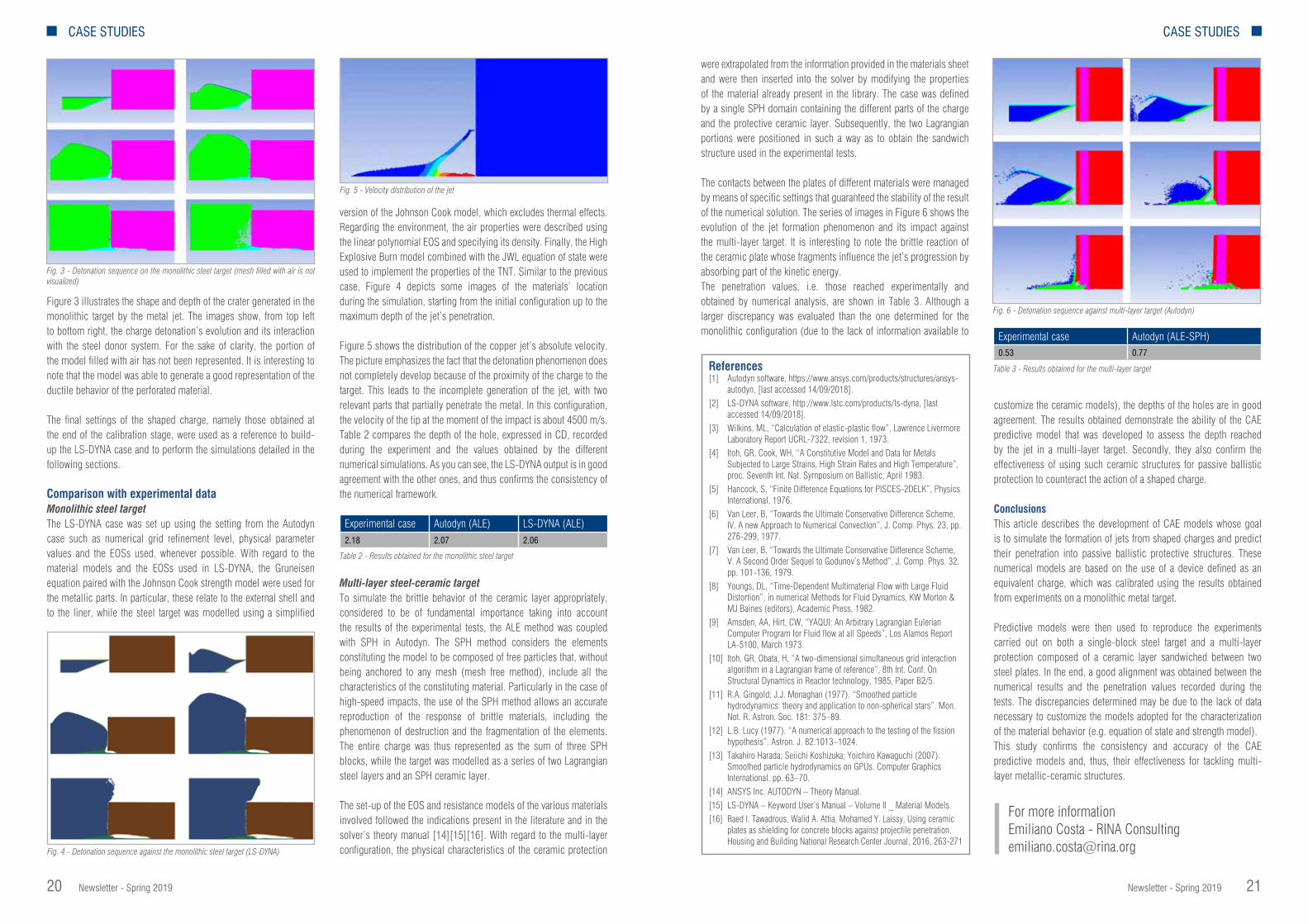
The contacts between the plates of different materials were managed by means of specific settings that guaranteed the stability of the result of the numerical solution. The series of images in Figure 6 shows the evolution of the jet formation phenomenon and its impact against the multi-layer target. It is interesting to note the brittle reaction of the ceramic plate whose fragments influence the jet’s progression by absorbing part of the kinetic energy. The penetration values, i.e. those reached experimentally and obtained by numerical analysis, are shown in Table 3. Although a larger discrepancy was evaluated than the one determined for the monolithic configuration (due to the lack of information available to
customize the ceramic models), the depths of the holes are in good agreement. The results obtained demonstrate the ability of the CAE predictive model that was developed to assess the depth reached by the jet in a multi-layer target. Secondly, they also confirm the effectiveness of using such ceramic structures for passive ballistic protection to counteract the action of a shaped charge.
ConclusionsThis article describes the development of CAE models whose goal is to simulate the formation of jets from shaped charges and predict their penetration into passive ballistic protective structures. These numerical models are based on the use of a device defined as an equivalent charge, which was calibrated using the results obtained from experiments on a monolithic metal target.
Predictive models were then used to reproduce the experiments carried out on both a single-block steel target and a multi-layer protection composed of a ceramic layer sandwiched between two steel plates. In the end, a good alignment was obtained between the numerical results and the penetration values recorded during the tests. The discrepancies determined may be due to the lack of data necessary to customize the models adopted for the characterization of the material behavior (e.g. equation of state and strength model). This study confirms the consistency and accuracy of the CAE predictive models and, thus, their effectiveness for tackling multi-layer metallic-ceramic structures.
For more informationEmiliano Costa - RINA [email protected]
References[1] Autodyn software, https://www.ansys.com/products/structures/ansys-
autodyn, [last accessed 14/09/2018].[2] LS-DYNA software, http://www.lstc.com/products/ls-dyna, [last
accessed 14/09/2018].[3] Wilkins, ML, “Calculation of elastic-plastic flow”, Lawrence Livermore
Laboratory Report UCRL-7322, revision 1, 1973.[4] Itoh, GR, Cook, WH, “A Constitutive Model and Data for Metals
Subjected to Large Strains, High Strain Rates and High Temperature”, proc. Seventh Int. Nat. Symposium on Ballistic, April 1983.
[5] Hancock, S, “Finite Difference Equations for PISCES-2DELK”, Physics International, 1976.
[6] Van Leer, B, “Towards the Ultimate Conservative Difference Scheme, IV. A new Approach to Numerical Convection”, J. Comp. Phys. 23, pp. 276-299, 1977.
[7] Van Leer, B, “Towards the Ultimate Conservative Difference Scheme, V. A Second Order Sequel to Godunov’s Method”, J. Comp. Phys. 32, pp. 101-136, 1979.
[8] Youngs, DL, “Time-Dependent Multimaterial Flow with Large Fluid Distortion”, in numerical Methods for Fluid Dynamics, KW Morton & MJ Baines (editors), Academic Press, 1982.
[9] Amsden, AA, Hirt, CW, “YAQUI: An Arbitrary Lagrangian Eulerian Computer Program for Fluid flow at all Speeds”, Los Alamos Report LA-5100, March 1973.
[10] Itoh, GR, Obata, H, “A two-dimensional simultaneous grid interaction algorithm in a Lagrangian frame of reference”, 8th Int. Conf. On Structural Dynamics in Reactor technology, 1985, Paper B2/5.
[11] R.A. Gingold; J.J. Monaghan (1977). “Smoothed particle hydrodynamics: theory and application to non-spherical stars”. Mon. Not. R. Astron. Soc. 181: 375–89.
[12] L.B. Lucy (1977). “A numerical approach to the testing of the fission hypothesis”. Astron. J. 82:1013–1024.
[13] Takahiro Harada; Seiichi Koshizuka; Yoichiro Kawaguchi (2007). Smoothed particle hydrodynamics on GPUs. Computer Graphics International. pp. 63–70.
[14] ANSYS Inc. AUTODYN – Theory Manual.[15] LS-DYNA – Keyword User’s Manual – Volume II _ Material Models.[16] Raed I. Tawadrous, Walid A. Attia, Mohamed Y. Laissy, Using ceramic
plates as shielding for concrete blocks against projectile penetration, Housing and Building National Research Center Journal, 2016, 263-271
Fig. 6 - Detonation sequence against multi-layer target (Autodyn)
Experimental case Autodyn (ALE-SPH)0.53 0.77
Table 3 - Results obtained for the multi-layer target
Figure 3 illustrates the shape and depth of the crater generated in the monolithic target by the metal jet. The images show, from top left to bottom right, the charge detonation’s evolution and its interaction with the steel donor system. For the sake of clarity, the portion of the model filled with air has not been represented. It is interesting to note that the model was able to generate a good representation of the ductile behavior of the perforated material.
The final settings of the shaped charge, namely those obtained at the end of the calibration stage, were used as a reference to build-up the LS-DYNA case and to perform the simulations detailed in the following sections.
Comparison with experimental dataMonolithic steel targetThe LS-DYNA case was set up using the setting from the Autodyn case such as numerical grid refinement level, physical parameter values and the EOSs used, whenever possible. With regard to the material models and the EOSs used in LS-DYNA, the Gruneisen equation paired with the Johnson Cook strength model were used for the metallic parts. In particular, these relate to the external shell and to the liner, while the steel target was modelled using a simplified
version of the Johnson Cook model, which excludes thermal effects. Regarding the environment, the air properties were described using the linear polynomial EOS and specifying its density. Finally, the High Explosive Burn model combined with the JWL equation of state were used to implement the properties of the TNT. Similar to the previous case, Figure 4 depicts some images of the materials’ location during the simulation, starting from the initial configuration up to the maximum depth of the jet’s penetration.
Figure 5 shows the distribution of the copper jet’s absolute velocity. The picture emphasizes the fact that the detonation phenomenon does not completely develop because of the proximity of the charge to the target. This leads to the incomplete generation of the jet, with two relevant parts that partially penetrate the metal. In this configuration, the velocity of the tip at the moment of the impact is about 4500 m/s.Table 2 compares the depth of the hole, expressed in CD, recorded during the experiment and the values obtained by the different numerical simulations. As you can see, the LS-DYNA output is in good agreement with the other ones, and thus confirms the consistency of the numerical framework.
Multi-layer steel-ceramic targetTo simulate the brittle behavior of the ceramic layer appropriately, considered to be of fundamental importance taking into account the results of the experimental tests, the ALE method was coupled with SPH in Autodyn. The SPH method considers the elements constituting the model to be composed of free particles that, without being anchored to any mesh (mesh free method), include all the characteristics of the constituting material. Particularly in the case of high-speed impacts, the use of the SPH method allows an accurate reproduction of the response of brittle materials, including the phenomenon of destruction and the fragmentation of the elements. The entire charge was thus represented as the sum of three SPH blocks, while the target was modelled as a series of two Lagrangian steel layers and an SPH ceramic layer.
The set-up of the EOS and resistance models of the various materials involved followed the indications present in the literature and in the solver’s theory manual [14][15][16]. With regard to the multi-layer configuration, the physical characteristics of the ceramic protection
Fig. 3 - Detonation sequence on the monolithic steel target (mesh filled with air is not visualized)
Fig. 4 - Detonation sequence against the monolithic steel target (LS-DYNA)
Fig. 5 - Velocity distribution of the jet
Experimental case Autodyn (ALE) LS-DYNA (ALE)2.18 2.07 2.06
Table 2 - Results obtained for the monolithic steel target

Newsletter - Spring 2019 2322 Newsletter - Spring 2019
CASE STUDIES CASE STUDIES
supply delays and higher production costs. Furthermore, automotive manufacturing customers are placing increasing attention on any aspects that do not directly affect the final quality of the product supplied because wastage and reworking waste energy, increasing the car manufacturer’s ecological footprint.Tolerances play a fundamental role in meeting both these sets of requirements. However, as a direct consequence of their small size and the amplifying effects typical of the propagation of tolerances, component manufacturers cannot limit the verification of these requirements only to the design rating.
The methodology developedIn complex products such as an OBC, the tolerances assigned to the individual parts propagate through the contacts and are amplified which can potentially impact heavily on the final product quality. It is, therefore, important to validate the design in advance and then verify it to pre-emptively predict their impact and mitigate the effects.The term “design validation” in this context thus referred to the calculations of the propagation of tolerances created during the design phase to predict whether and how much the tolerances would affect the ability to meet the product requirements, prior to prototyping the first components. Armed with this information, the designers can intervene with corrective actions to improve the quality of the final product.By nature, these calculations are complex and three-dimensional and require the use of dedicated software to obtain reliable results in a reasonable amount of time for industry. For these reasons, EnginSoft uses Cetol 6σ, developed by US-based Sigmetrix, to undertake these projects.
A further consideration that should not be underestimated is the geometric specification of the products: in recent years, the standards ISO 1101:2017, ISO 8015:2011, and ASME Y14.5-2018, which describe the geometric and dimensional variability of the tolerances represented in technical drawings, have been updated. The resulting geometric dimensioning and tolerancing (GD&T) language makes it possible to functionally describe components unambiguously. This is fundamental for tolerance propagation calculations that quantify quality because it enables the generation of unquestionable results. The use of this language is therefore integral to the methodology.
During “design verification”, the real measurements of the prototype parts, produced from the models created during the “design validation” phase, were inserted into the software for the purposes of data reusability. This phase will enable designers to verify virtually (and therefore immediately), the impact of any aspect that is “out of tolerance” and quantify its effect on final quality. This will then enable informed decisions to be made about any corrective actions to be taken to avoid contestation of the supply by the customer.
The success of this phase is determined by the dimensional controls. In particular, the measurements must be taken in accordance with the project specifications. The use of the GD&T’s standardized and unambiguous syntax also facilitates this, resulting in dimensional
and geometric descriptions that are, by nature, suitable for evaluation with particular tools such as coordinate measuring machines (CMM), 3D optical scanners, or laser systems that accurately describe the surfaces by generating point clouds. Instrumentation then acquires these point clouds which are processed by the software, allowing the designer to “align” the scan of the actual part with its ideal model (a 3D CAD) to assess its compliance with the design tolerances.
Results and conclusionsBy applying the method developed and using the tools proposed, Metasystem was able to demonstrate the “robustness” of the project (defined as the low sensitivity of the requirements to the geometric and dimensional variations granted by the tolerances) to the customer and to fulfil all the requirements described.
This was achieved by interventions at the design phase, by making minor modifications to the nominal CAD geometries, and by working with the tolerances using GD&T standards-compliant dimensioning drawings.The ultimate aim of the design validation phase is to table designs that, if respected, will guarantee the desired quality of the assembled product at the lowest possible cost based on the capability of the available production process.
It is highly likely that other customers will approach Metasystem with similar OBC design requirements, which would necessitate the repetition of these activities and calculations. Consequently, the consolidation of the methodology and the acquisition of suitable verification tools can be considered a competitive advantage for Metasystem: the project has allowed the company to acquire the know-how to satisfy future customer requests on the one hand, and to create projects that are as profitable as possible in terms of waste minimization, on the other hand.
For more informationEnrico Boesso - [email protected]
Globally, the automotive industry is striving to reduce CO2 emissions to meet increasingly stringent environmental protection standards. Car manufacturers are intensifying their research and development of hybrid and electric motors. These products require highly reliable, efficient subsystems to manage their electrical energy. The on-board charger (OBC) is one of the key components in the energy efficiency of these vehicles.The OBC is a compact battery charger for electric vehicles that converts the alternate voltage supplied by the mains into the direct voltage used to charge the vehicle’s high traction voltage battery. OBC Metasystems are products that take into account weight, costs, space, power density and efficiency and which must apply international standards and meet the functional safety requirements of ISO26262.
Electro-mechanical integration and the role of tolerances in the product requirementsA complex product such as an OBC must meet various requirements, some relating to the mechanics involved and others to the electro-mechanical integration. These are explicitly requested by the customer who also requires visible compliance during the entire product development cycle.
To obtain high levels of efficiency, the weight and dimensions must be kept within pre-established limits. For the product, this leads to a
high-density placement of electronic components inside and adjacent to the conductive structural elements, such as the aluminum housing, which dramatically increases the risk of discharges, short circuits, bridges, air creepage, etc. This can cause malfunctions, higher risk of fire, and lower efficiency which compromise the reliability of the system. To prevent these repercussions, designers identify, isolate and shield the areas at greatest risk, an approach known as the “insulation concept”. For the manufacturer, this demand for reduced dimensions increases the risk of interference during assembly which can cause an automatic assembly line to shut down, leading to loss of productivity,
Development of a methodology and tools for tolerances in vehicle electrification to meet future customer demand and ensure competitive advantage EnginSoft and Metasystem develop design validation, verification methodology for high-performance on-board chargers for electric vehicles
By Enrico Boesso1, Gabriele Codeluppi21. EnginSoft - 2. Metasystem
CASE STUDIES
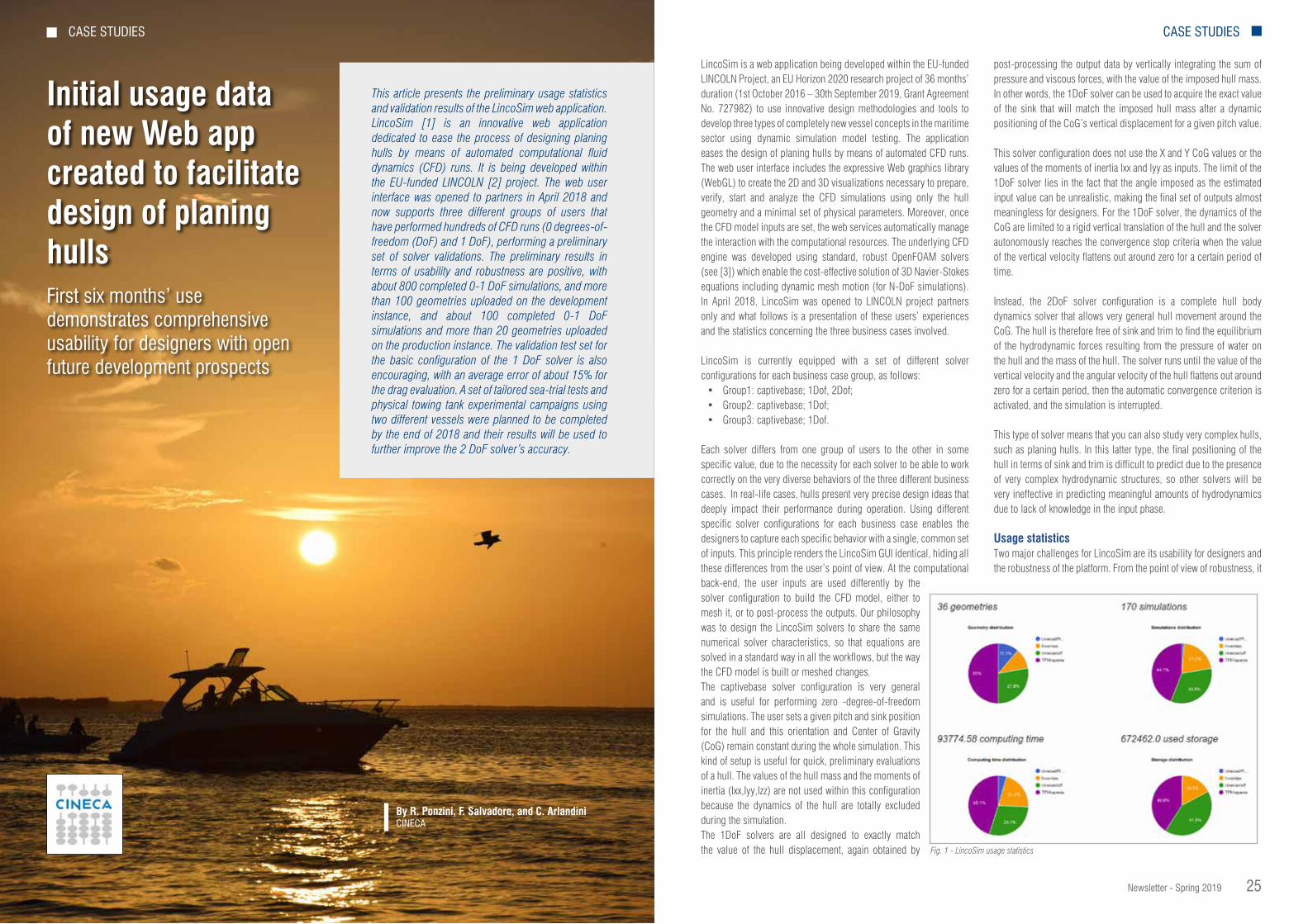
Newsletter - Spring 2019 2524 Newsletter - Spring 2019
CASE STUDIES CASE STUDIES
Initial usage data of new Web app created to facilitate design of planing hulls First six months’ use demonstrates comprehensive usability for designers with open future development prospects
By R. Ponzini, F. Salvadore, and C. Arlandini CINECA
This article presents the preliminary usage statistics and validation results of the LincoSim web application. LincoSim [1] is an innovative web application dedicated to ease the process of designing planing hulls by means of automated computational fluid dynamics (CFD) runs. It is being developed within the EU-funded LINCOLN [2] project. The web user interface was opened to partners in April 2018 and now supports three different groups of users that have performed hundreds of CFD runs (0 degrees-of-freedom (DoF) and 1 DoF), performing a preliminary set of solver validations. The preliminary results in terms of usability and robustness are positive, with about 800 completed 0-1 DoF simulations, and more than 100 geometries uploaded on the development instance, and about 100 completed 0-1 DoF simulations and more than 20 geometries uploaded on the production instance. The validation test set for the basic configuration of the 1 DoF solver is also encouraging, with an average error of about 15% for the drag evaluation. A set of tailored sea-trial tests and physical towing tank experimental campaigns using two different vessels were planned to be completed by the end of 2018 and their results will be used to further improve the 2 DoF solver’s accuracy.
LincoSim is a web application being developed within the EU-funded LINCOLN Project, an EU Horizon 2020 research project of 36 months’ duration (1st October 2016 – 30th September 2019, Grant Agreement No. 727982) to use innovative design methodologies and tools to develop three types of completely new vessel concepts in the maritime sector using dynamic simulation model testing. The application eases the design of planing hulls by means of automated CFD runs. The web user interface includes the expressive Web graphics library (WebGL) to create the 2D and 3D visualizations necessary to prepare, verify, start and analyze the CFD simulations using only the hull geometry and a minimal set of physical parameters. Moreover, once the CFD model inputs are set, the web services automatically manage the interaction with the computational resources. The underlying CFD engine was developed using standard, robust OpenFOAM solvers (see [3]) which enable the cost-effective solution of 3D Navier-Stokes equations including dynamic mesh motion (for N-DoF simulations). In April 2018, LincoSim was opened to LINCOLN project partners only and what follows is a presentation of these users’ experiences and the statistics concerning the three business cases involved.
LincoSim is currently equipped with a set of different solver configurations for each business case group, as follows:
• Group1: captivebase; 1Dof, 2Dof;• Group2: captivebase; 1Dof;• Group3: captivebase; 1Dof.
Each solver differs from one group of users to the other in some specific value, due to the necessity for each solver to be able to work correctly on the very diverse behaviors of the three different business cases. In real-life cases, hulls present very precise design ideas that deeply impact their performance during operation. Using different specific solver configurations for each business case enables the designers to capture each specific behavior with a single, common set of inputs. This principle renders the LincoSim GUI identical, hiding all these differences from the user’s point of view. At the computational back-end, the user inputs are used differently by the solver configuration to build the CFD model, either to mesh it, or to post-process the outputs. Our philosophy was to design the LincoSim solvers to share the same numerical solver characteristics, so that equations are solved in a standard way in all the workflows, but the way the CFD model is built or meshed changes.The captivebase solver configuration is very general and is useful for performing zero -degree-of-freedom simulations. The user sets a given pitch and sink position for the hull and this orientation and Center of Gravity (CoG) remain constant during the whole simulation. This kind of setup is useful for quick, preliminary evaluations of a hull. The values of the hull mass and the moments of inertia (Ixx,Iyy,Izz) are not used within this configuration because the dynamics of the hull are totally excluded during the simulation.The 1DoF solvers are all designed to exactly match the value of the hull displacement, again obtained by
post-processing the output data by vertically integrating the sum of pressure and viscous forces, with the value of the imposed hull mass. In other words, the 1DoF solver can be used to acquire the exact value of the sink that will match the imposed hull mass after a dynamic positioning of the CoG’s vertical displacement for a given pitch value.
This solver configuration does not use the X and Y CoG values or the values of the moments of inertia Ixx and Iyy as inputs. The limit of the 1DoF solver lies in the fact that the angle imposed as the estimated input value can be unrealistic, making the final set of outputs almost meaningless for designers. For the 1DoF solver, the dynamics of the CoG are limited to a rigid vertical translation of the hull and the solver autonomously reaches the convergence stop criteria when the value of the vertical velocity flattens out around zero for a certain period of time.
Instead, the 2DoF solver configuration is a complete hull body dynamics solver that allows very general hull movement around the CoG. The hull is therefore free of sink and trim to find the equilibrium of the hydrodynamic forces resulting from the pressure of water on the hull and the mass of the hull. The solver runs until the value of the vertical velocity and the angular velocity of the hull flattens out around zero for a certain period, then the automatic convergence criterion is activated, and the simulation is interrupted.
This type of solver means that you can also study very complex hulls, such as planing hulls. In this latter type, the final positioning of the hull in terms of sink and trim is difficult to predict due to the presence of very complex hydrodynamic structures, so other solvers will be very ineffective in predicting meaningful amounts of hydrodynamics due to lack of knowledge in the input phase.
Usage statisticsTwo major challenges for LincoSim are its usability for designers and the robustness of the platform. From the point of view of robustness, it
Fig. 1 - LincoSim usage statistics
CASE STUDIES

Newsletter - Spring 2019 2726 Newsletter - Spring 2019
CASE STUDIES CASE STUDIES
is necessary to consider the robustness of the software of the devised platform and the hardware of both the virtual machines hosting the Web services and the connected high-performance computing (HPC) clusters. In addition, there is the difficult task concerning the robustness of the CFD solver. From a usage point of view, the transition from a carefully designed and implemented architecture to real-world use is a clear challenge. This section provides some statistical data that is being used to assess LincoSim after its first 6 months in production.
The LincoSim service uptime, or the reachability of the web-page https://lincosim.cineca.it, which includes the uptime of both the virtual machine as well as the operations of the web-server software stack, was 99.2%. Even considering that this is a completely custom software architecture, it is a very good result.
With regard to the effective functioning of the HPC cluster used, i.e. the Galileo cluster at Cineca (see http://www.hpc.cineca.it/hardware/galileo-0) the analysis is more difficult because very specific difficulties can render some jobs not correctly operational. Fortunately, during these first six months of production, such events involving LincoSim have been very rare, and have been fairly transparently managed for users by the LincoSim staff.
Regarding the assignment of HPC resources, the three nodes reserved on the cluster and managed by a state-of-the-art job scheduler used
by many of the world’s supercomputers (Slurm Workload Manager)guaranteed very short wait-times for the jobs (normally within 24 hours), except in the last two weeks of the period in which a peak in requests led to a delay of a few days in the completion of all jobs submitted. Apart from this delay, everything was managed by the platform in a completely transparent way for the user.
For completeness, we report some statistics here regarding the actual use of the platform, relating to both active instances of LincoSim: the development one used internally for testing new features and developing new simulation setups, and the production one used directly by users and active since April 2018 (see Table 1).
For the production instance, we have also reported the statistics on the use of resources by the various organizations included in the LincoSim project.
Overall, we believe that in its first six months of production, LincoSim has had a positive response regarding usage from the various partners. In addition to what has been reported here, several exchanges with partners have shown that the platform is comprehensively usable by the type of user for which it was designed. Future development prospects also remain open in view of the innovative approach that has been taken.
It is also interesting to compare the time trend of the number of simulations launched each month for the two instances. The peaks of the development instance correspond to the periods of greatest intensity of the solver tests, with attention to the generic approach used in addition to the quality of the results (see Figure 2).
ConclusionsStarting from April 2018, the LincoSim web application was opened to three groups of industrial partners involved in the LINCOLN project and it has been massively used to support the design process of innovative vessels by means of automatic CFD runs. The preliminary statistical results in terms of usability and robustness are really encouraging. Hundreds of simulations have been carried out by non-expert users in a few months. Nonetheless, we are now undertaking full validation tests to more properly assess the application’s accuracy by referencing towing tank data. This last activity, planned for completion by September 2019, should provide a meaningful benchmark on the real effectiveness of the tool.
For more informationRaffaele Ponzini - CINECA [email protected]
References[1] LincoSim web access (only for registered users):
http://www.hpc.cineca.it/hardware/galileo-0 [2] LINCOLN project web site: http://www.lincolnproject.eu/ [3] OpenFOAM web site: https://openfoam.org/
Fig. 2 - Close-up of complex wing-tip surfaces showing before (red) and morphed (blue) surfaces
Quantity LincoSim development
LincoSim production
# organizations 6 6
# users 8 25
# geometries 101 36
# simulations 834 170
# simulations setups 32 5
# HPC machines 6 1
computing time [core-hours] 211,716.55 93,774.58
storage [GB] 2,028,227.0 672,462.0
Table1: LincoSim usage statistics
Matter-radiation interaction is relevant in several industrial applications. Accurate interaction modelling using correct radiation parameters is essential to predict the physical behavior of used materials, such as their fatigue lifetime. In this article, we present a procedure to investigate the thermo-mechanical effects produced by the particles of an extremely focused beam hitting a material target spot. The work is based on a multi-purpose script created with ANSYS APDL code. The APDL features made it possible to simulate the temperature and the strain of the target based on specific physical parameters, and on the spatial and temporal distributions of radiation beam particles, while also extending the results to a high number of thermal cycles to investigate the fatigue lifetime. The script was developed during the theoretical investigation of the interaction between optical transition radiation (OTR) screens and the electron beams of the ELI-NP Gamma Beam Source facility. In this case study, the simulated electron beam consists of trains of 32 electron bunches of 250 pC each, separated by 16 ns and distributed along a 0.5 μs RF pulse with a repetition rate of 100 Hz.
The most diffuse particle beam in modern industry is the electron beam. It is implemented in a wide spectrum of industrial applications in different fields, such as welding, biological sterilization, microscopy, machining, additive manufacturing, physical vapor deposition, as well as in research facilities for nuclear physics experiments. For all the above-mentioned branches, the control of the beam parameters and their related interaction with target materials are crucial for the effective and efficient functioning of equipment. Just to give an example, in electron beam welding processes, the evaluation of the heat affected zone (HAZ) is extremely important to finely tune the beam parameters regarding material type and geometry, to minimize the degradation of mechanical material performance in that zone (e.g. brittleness, and reduction of mechanical strength). The methodology proposed here could be extremely useful in the industrial field, with increasingly varied areas of application emerging in the future. In addition to the current most common applications of the electron beam already mentioned, there are more advanced processes that aim to produce “greener” parts, cheaper and faster than more traditional techniques. Among these, for example, are the deposition of chemicals, the irradiation of materials for several purposes (food and medicine included), and the most advanced analytical techniques
Multi-purpose ANSYS APDL script developed
for analysis of matter-radiation
interaction Ability to predict thermal and
mechanical behavior within specific physical parameters has multiple
industrial applications
By F. Cioeta1, D. Alesini1, M. Ciambrella2, D. Cortis1, M. Marongiu1, A. Mostacci2, V. Pettinacci1 and A. Variola1
1. National Institute for Nuclear Physics (INFN)2. Department of Basic and Applied Sciences for Engineering of the Sapienza University of Rome

Newsletter - Spring 2019 2928 Newsletter - Spring 2019
CASE STUDIES CASE STUDIES
a continuous oscillating change of the temperature distribution. In order to evaluate this distribution during the temperature heating and decreasing (thermal cycle) of the OTR, used for the beam diagnostic, several thermal transient analyses were performed. The OTR target’s geometry (30 mm long for each edge and 1 mm thick) was modelled with 3D SOLID70 elements [2] using a dedicated FE code in ANSYS APDL [2]. Moreover, a refinement of the mesh (Fig.1, darker area) was applied close to the electron beam spot where the heat generation is concentrated (minimum size of the mesh elements 6x10⁻⁶ m) to obtain a correct distribution of the power density resulting from the beam-target interaction.
The ANSYS APDL code applies the thermal load to those mesh elements that correspond to the portion of the OTR target that significantly interacts with the electron beam. The worst-case scenario was considered to be an elliptical beam spot that corresponded to the more focused beam (Fig.1).
OTR screenThe OTR is the radiation emitted when a fast particle crosses the boundary between two media with a different dielectric constant. This light is emitted with a characteristic angular distribution that depends on the particle energy and the angular momentum [5]. The particle’s electro-magnetic field has a certain configuration in the vacuum in
front of the foil, which differs from the one of the field inside the media, because the foil’s dielectric constant is different from vacuum’s. When approaching the foil, the particle’s electro-magnetic field creates a time-dependent polarization at the foil boundary. The change of this polarization causes the radiation with a characteristic intensity and angular distribution.
A typical setup of an OTR measurement is shown in Fig. 2. In most cases, the foil is inserted at a 45° angle to the beam path. The foil is typically made of aluminized silicon with a thickness in the order of tens of micrometers. The light is emitted both in the forward direction and at 90° because the metallic surface acts as a mirror. Depending on the particle energy, the angular distribution is peaked at the angle θ=1⁄γ where γ is the relativistic Lorentz factor.
The light that is emitted at 90° was acquired with appropriate optics, and an image of the foil was recorded with a charge-coupled device (CCD) camera. This is useful to measure some important properties of the beam: indeed, one can directly measure the transverse spot size. Moreover, using a quadrupole scan technique, it is possible to measure the beam’s emittance; while an RF Deflector makes it possible to retrieve the bunch length and, combined with a dipole, to generate the complete 6D characterization of the beam. Additionally, by acquiring the OTR angular distribution (focus on infinity), it is possible to measure the beam’s energy and divergence.
APDL script structureThe APDL script is structured in three main parts. The first refers to the definition of the electron beam’s properties and the OTR target’s material and geometry. The second spatially models the power density resulting from the interaction between the electron beam and the target. The third models the power density over time, assuming a pulsed operation mode for the beam described in section 3 and by simulating a high number of thermal cycles on the target material using a specific configuration of the ANSYS solver code (i.e. load steps in Fig. 3). These three parts are described in detail below, although the well-known parts of post-processing a FEM simulation have been omitted.
Definition of beam and OTR target properties The APDL script supports three kinds of parameters: “variable”, “array” and “table”. This latter is a special type of multi-dimensional array that allows ANSYS to calculate the values between the array elements through linear interpolation.
Every physical property, from the electron beam’s characteristics to the geometric dimensions and the material properties of the OTR target, becomes a parameter of the simulation and is modelled as an ANSYS variable. These variables are defined in the pre-processing section of the APDL script, as is usual in FEM analysis. The parametrization of the physical problem allows one to easily tailor the simulations to specific user cases and to execute a sensitivity analysis to tune the beam and/or the equipment properties to achieve the best system performance. Fig. 2 - OTR screen placed at 45° with respect to beam axis [5]
Fig. 1 - OTR screen and hotspot 3D mesh
for the internal structure of materials (tomography). Another important field of application is the heat treatment (cure) of metals for aircraft, automobiles and recreational equipment, which uses this technology to reduce the time and costs of the process [1]. For any one of the previous examples, electron beams (i.e. the energy and therefore power applied) and materials are different, but by means of the code we present here, it becomes possible to control the temperature distribution of the mechanical part treated and to consequently properly evaluate the stress induced.
This article is presented in five parts. In the first part, we introduce a numerical methodology, based on the ANSYS Parametric Design Language (APDL), to investigate the thermal effects resulting from the interaction of an electron bunched beam hitting a general material surface. The APDL script developed was used to predict the thermal-mechanical behavior of the electron beam diagnostic device, which to be mounted on the beam line of a nuclear research facility (the Extreme Light Infrastructure – Nuclear Physics (ELI-NP)).
The second part of the article describes the main capabilities of the APDL and the reasons why it is essential to properly investigate the thermo-mechanical effects of the interactions between a particle beam and a target material. The third part illustrates the real case study which focused on setting a beam diagnostic device, the Optical Transient Radiation (OTR) screen. The fourth part outlines the APDL script developed, while the fifth and last section of the article reports the results of the thermal transient simulations that were performed for the OTR screen using the APDL script.
The capabilities of the ANSYS parametric design language (APDL) codeThe APDL is a scripting language that can be used to automate common tasks or build a finite element model (FEM) using parameters (variables). The code has many features such as repeating a command, macros, if-then-else branching, do-loops, and scalar, vector and matrix operations [2]. Its main difference from the ANSYS Workbench environment is the complete control it offers users of the model – both at the pre-processing (data input) and post-processing (results extrapolation) phases – with the possibility of writing the entire program in batch mode, as opposed to the click mode of a graphical user interface (GUI). This feature means that the APDL applications are limited only by the user’s mind and no longer by the GUI functionality.
Particle beams lose energy as heat when interacting with a target material, generating a (thermal) power density inside the latter. Particles, in our case electrons, are not distributed uniformly along the transverse sections of the beam, but according to a Gaussian distribution; consequently, the power density generated is not spatially uniform on the target surface either, but Gaussian as well. Moreover, when the beam is pulsed, the power density generated is not constant over the time, but has a cyclic trend, going from zero to
a maximum peak. In our case study, the electron beam was not only pulsed but also had a very high frequency of 100 Hz, which was the same as that of the power density generated.
The ANSYS Workbench GUI does not allow users to simulate this kind of thermal problem, whereas the development of an opportune APDL script does. Moreover, an APDL script allows the parametrization of the physical radiation variables and material characteristics. In our case, the parametrization was done by writing external custom data files containing the information to be used by the APDL script, depending on the type of simulation, while repeated actions (such as the load steps for simulating the power density trend), do-loops, mathematical formulas and matrixes were programmed directly inside the main scripting code. Furthermore, writing the entire program in batch mode allowed optimal management of memory usage by saving only the useful data for each simulation.
Finally, the choice to use the APDL environment was driven by the distribution of the particles of the beam to be simulated in the case study, since they reflected a peculiar spatial and time distribution of the power density in the target material. The APDL script developed may also easily be adapted to suit other applications involving different specific beams, material and setting geometries.
Case study: the Optical Transition Radiation (OTR)screen of a nuclear research facilityThe APDL script was developed during the investigation of the interactions between the OTR screens and electron beams designed for the ELI-NP Gamma Beam System (GBS) facility – an advanced source of up to ≈ 20 MeV gamma rays based on Compton back scattering, i.e. the collision of an intense high-power laser beam and a high-brightness electron beam with a maximum kinetic energy of about 740 MeV. In this case study, the simulated electron beam consists of trains of 32 electron bunches of 250 pC each, separated by 16 ns and distributed along a 0.5 μs RF pulse with a repetition rate of 100 Hz [3].
The analysis was developed starting from previous theoretical analysis results [4] that were used as input for the FE simulations to evaluate the thermal and mechanical performance of two candidate materials for the target (i.e. aluminum and monocrystalline silicon), especially under a high number of thermal cycles, with the objective of choosing the best-performing one.
This methodology takes into account the most demanding operating conditions of the GBS machine: indeed, along the linear accelerator (LINAC), the electron beam is symmetric but in a particular position, at more or less 13 meters from the gun, the electron beam becomes asymmetric with an elliptical shape, where σx is the beam size along the x-axis equal to 47.5x10⁻⁶ m and σy is the beam size along the y-axis equal to 109.0x10⁻⁶ m.
In this condition, the beam has a high charge density and the impact on the target produces a different behavior in the temperature i.e.
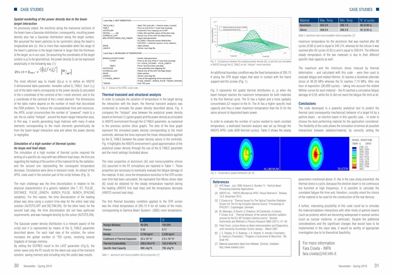
Newsletter - Spring 2019 3130 Newsletter - Spring 2019
CASE STUDIES CASE STUDIES
An additional boundary condition was the fixed temperature of 295.15 K along the OTR target edges that were in contact with the frame support and the screws (Fig. 1).
Fig. 5 represents the spatial thermal distribution (x, y) when the beam hotspot reaches the maximum temperature for both materials in the first thermal cycle. The Si has a higher and a more spatially concentrated ∆T respect to the Al. The Al has a higher specific heat capacity and thus a lower maximum temperature than the Si for the same amount of deposited beam power.
In order to evaluate the number of cycles needed to reach constant temperature, a dedicated transient analysis was set up through the ANSYS APDL code (600 thermal cycles). Table 2 shows the steady
maximum temperature for the aluminum that was reached after 80 cycles (0.80 s) and is equal to 345.3 K, whereas for the silicon it was reached after 92 cycles (0.92 s) and is equal to 358.9 K. The different steady temperature of the two materials is due to their different specific heat capacity as well.
The maximum and the minimum stress induced by thermal deformation – and calculated with this code – were then used to evaluate fatigue and related lifetime. Al reaches a Goodman alternate stress of 30.20 MPa whereas the Si reaches 7.74 MPa. After one hour of exposition (36,000 cycles) – taking into account the related Wöhler curves for each material – the Al reached a cumulative fatigue damage of 0.59, while the Si did not reach the fatigue life limit at all.
ConclusionsThe code developed is a powerful analytical tool to predict the thermal (and consequently mechanical) behavior of a target hit by a particle beam – an electron beam in this specific case – in order to choose the best-performing material for the application considered. The flexibility of the code allows the simulation of almost all possible interactions between radiation/material, by correctly setting the
parameters mentioned above. If, like in the case study presented, the thermal stress is cyclic (because the electron beam is not continuous but bunched at high frequency), it is possible to calculate the correlated fatigue life-time and, therefore, crucially orient the choice of the material to be used for the construction of the real devices.
A further, interesting possibility of this code could be to simulate the material/radiation interactions with other kinds of particle beams (such as protons) which are becoming widespread in several sectors (such as nuclear medicine, in particular). Despite the additional considerations and the significant changes that would have to be implemented in the input data, it would be worthy of appropriate investigation due to its theoretical feasibility.
For more informationFara Cioeta - [email protected]
References[1] APS News - July 1996 (Volume 5, Number 7) - Particle Beam
Processing Industrial Applications. [2] ANSYS Inc., “ANSYS Mechanical APDL Theory Reference”, Release
15.0, November 2013.[3] F.Cioeta et al. “Thermal Issues For The Optical Transition Radiation
Screen For The Eli-Np Compton Gamma Source” Proceedings of IPAC2017, Copenhagen, Denmark.
[4] M. Marongiu, D.Alesini, E.Chiadroni, M.Ciambrella, A.Cianchi, F.Cioeta, et al. “ Thermal behavior of the optical transition radiation screens for the ELI-NP Compton Gamma source”. Nuclear Instruments and Methods in Physics Research A865 (2017), 47–50.
[5] Peter Forck, Lecture Notes on Beam Instrumentation and Diagnostics, Joint University Accelerator School January – March 2007.
[6] J. E. Shigley, R. G. Budynas, J. K. Nisbett, D. Amodio (Translator), G. Santucci (Translator), “Progetto e Costruzione di Macchine”, Mc Graw Hill.
[7] Material parameters taken from Matweb. [Online]. Available: http://www.matweb.com/.
Fig. 4 - Comparison between the analytical power density Q(x, y) and the one simulated in ANSYS through the Q_TABLE on the “hotspot” mesh elements
Fig. 5 - Temperature spatial distribution (Al, Si)
Material Max. Temp. Min. Temp. N° of cyclesAluminium 345.3 K 296.1 K 80 (0.80 s)
Silicon 358.9 K 296.3 K 92 (0.92 s)
Table 1: aluminum and monocrystalline silicon properties [7]
Spatial modelling of the power density due to the beam target interactionAs previously stated, the electrons along the transverse sections of the beam have a Gaussian distribution; consequently, resulting power density also has a Gaussian distribution along the target surface. We assumed the beam particles to be symmetric along the beam’s longitudinal axis (z): this is more than reasonable when the range of the beam’s particles in the target material is larger than the thickness of the target, as in our case. On assuming the coordinates of the target surface (x,y) to be geometrical, the power density Q can be expressed analytically in the following way (1):
The most efficient way to model Q(x,y) is to define an ANSYS 2-dimensional table parameter, hereafter called Q_TABLE. Each (i,j) cell of the table matrix corresponds to the power density Q calculated in the x-coordinate of the centroid of the i-mesh element, and in the y-coordinate of the centroid of the j-mesh element. The dimensions of the table matrix depend on the number of mesh that discretized the FEM problem. To reduce the computational time and resources, the APDL script circumscribes the number of “powered” mesh to a set, the so-called “hotspot”, around the beam-target interaction area. In this way, it avoids generating huge matrixes with many 0-value elements corresponding to the mesh elements geometrically far from the beam-target interaction area and where the power density is negligible.
Simulation of a high number of thermal cycles: do-loops and load stepsThe simulation of a high number of thermal cycles required the writing of a specific do-loop with two different load steps: the first one regarding the heating of the portion of the material hit by the radiation, and the second one representing the consequent temperature decrease. Simulations were done in transient mode. An extract of the APDL code used in the solution part of the script follows (Fig. 3).
The main challenge was the time discretization in relation to the physical characteristics of a generic radiation (the T, DT, PULSE_DISTANCE, PULSE_LENGTH, BUNCH_PULSE, BUNCH_SPACING variables). For this reason, the time discretization of the heating phase was done using a custom time-step for the entire load step solution (AUTOTS,OFF and DELTIM,ON). On the other hand, for the second load step, the time discretization did not have particular requirements, and was managed directly by the solver (AUTOTS,ON).
The Gaussian power density distribution is a relevant aspect of the script and it is represented by means of the Q_TABLE parameter described above. For each load step of the solution, the solver increases the global number of *DO cycles, involving several Gigabyte of storage memory. By setting the OUTRES result to the LAST parameter (Fig.3), the solver saves only the FE results for the latest sub-step of the transient solution, saving memory and including only the useful data results.
Thermal transient and structural analysisIn order to evaluate the variation of temperature in the target during the interaction with the beam, the thermal transient analysis was conducted to simulate the power density described above. Fig. 4 compares the “hotspot” area between the analytical power density based on formula (1) (green graph) and the power density as simulated in ANSYS environment through the Q TABLE parameter, as explained in the previous section (blue graph). The dots of the blue graph represent the simulated power density corresponding to the mesh centroids, whereas the lines represent the linear interpolation applied by the Q_TABLE between the power density values in the centroids. Fig. 4 highlights the ANSYS environment’s good approximation of the analytical power density through the use of the Q TABLE parameter and the mesh settings illustrated above.
The main properties of aluminum (Al) and monocrystalline silicon (Si) assumed in the FE simulations are reported in Table 1. These properties are necessary to eventually evaluate the fatigue damage of the material. In fact, once the temperature evolution in the OTR screen over time had been calculated, the equivalent Von Mises stress state [6] could be obtained for the steady temperature reached during the heating (ANSYS first load step) and the temperature decrease (ANSYS second load step).
The first thermal boundary condition applied to the OTR screen was the initial temperature of 295.15 K for all nodes of the mesh, corresponding to Gamma Beam System/- (GBS) room temperature.
Al SiYoung's Modulus 69 GPa 150 GPa
Poisson 0.33 0.17
Density 2,700 kg/m3 2,330 kg/m3
Coefficient of Thermal Expansion 23 x 10-6 K-1 2.5 x 10⁻⁶ K-1
Thermal Conductibility 209.0 W/m*K 143.5 W/m*K
Specific Heat Capacity 890 J/kg*K 700 J/kg*K
Table 1 - aluminum and monocrystalline silicon properties [7]
Fig. 3 - Extract of the APDL script code
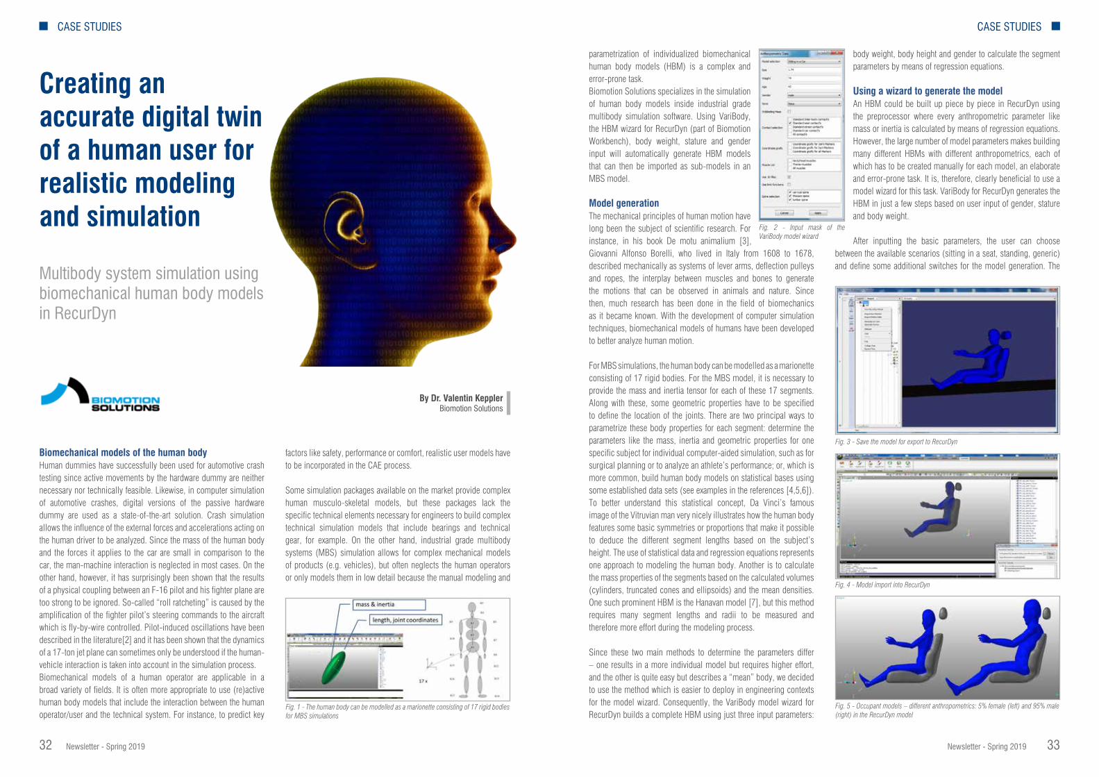
Newsletter - Spring 2019 3332 Newsletter - Spring 2019
CASE STUDIES CASE STUDIES
Biomechanical models of the human body Human dummies have successfully been used for automotive crash testing since active movements by the hardware dummy are neither necessary nor technically feasible. Likewise, in computer simulation of automotive crashes, digital versions of the passive hardware dummy are used as a state-of-the-art solution. Crash simulation allows the influence of the external forces and accelerations acting on the human driver to be analyzed. Since the mass of the human body and the forces it applies to the car are small in comparison to the car, the man-machine interaction is neglected in most cases. On the other hand, however, it has surprisingly been shown that the results of a physical coupling between an F-16 pilot and his fighter plane are too strong to be ignored. So-called “roll ratcheting” is caused by the amplification of the fighter pilot’s steering commands to the aircraft which is fly-by-wire controlled. Pilot-induced oscillations have been described in the literature[2] and it has been shown that the dynamics of a 17-ton jet plane can sometimes only be understood if the human-vehicle interaction is taken into account in the simulation process.Biomechanical models of a human operator are applicable in a broad variety of fields. It is often more appropriate to use (re)active human body models that include the interaction between the human operator/user and the technical system. For instance, to predict key
factors like safety, performance or comfort, realistic user models have to be incorporated in the CAE process.
Some simulation packages available on the market provide complex human musculo-skeletal models, but these packages lack the specific technical elements necessary for engineers to build complex technical simulation models that include bearings and technical gear, for example. On the other hand, industrial grade multibody systems (MBS) simulation allows for complex mechanical models of products (e.g. vehicles), but often neglects the human operators or only models them in low detail because the manual modeling and
parametrization of individualized biomechanical human body models (HBM) is a complex and error-prone task. Biomotion Solutions specializes in the simulation of human body models inside industrial grade multibody simulation software. Using VariBody, the HBM wizard for RecurDyn (part of Biomotion Workbench), body weight, stature and gender input will automatically generate HBM models that can then be imported as sub-models in an MBS model.
Model generation The mechanical principles of human motion have long been the subject of scientific research. For instance, in his book De motu animalium [3], Giovanni Alfonso Borelli, who lived in Italy from 1608 to 1678, described mechanically as systems of lever arms, deflection pulleys and ropes, the interplay between muscles and bones to generate the motions that can be observed in animals and nature. Since then, much research has been done in the field of biomechanics as it became known. With the development of computer simulation techniques, biomechanical models of humans have been developed to better analyze human motion.
For MBS simulations, the human body can be modelled as a marionette consisting of 17 rigid bodies. For the MBS model, it is necessary to provide the mass and inertia tensor for each of these 17 segments. Along with these, some geometric properties have to be specified to define the location of the joints. There are two principal ways to parametrize these body properties for each segment: determine the parameters like the mass, inertia and geometric properties for one specific subject for individual computer-aided simulation, such as for surgical planning or to analyze an athlete’s performance; or, which is more common, build human body models on statistical bases using some established data sets (see examples in the references [4,5,6]). To better understand this statistical concept, Da Vinci’s famous image of the Vitruvian man very nicely illustrates how the human body features some basic symmetries or proportions that make it possible to deduce the different segment lengths based on the subject’s height. The use of statistical data and regression equations represents one approach to modeling the human body. Another is to calculate the mass properties of the segments based on the calculated volumes (cylinders, truncated cones and ellipsoids) and the mean densities. One such prominent HBM is the Hanavan model [7], but this method requires many segment lengths and radii to be measured and therefore more effort during the modeling process.
Since these two main methods to determine the parameters differ – one results in a more individual model but requires higher effort, and the other is quite easy but describes a “mean” body, we decided to use the method which is easier to deploy in engineering contexts for the model wizard. Consequently, the VariBody model wizard for RecurDyn builds a complete HBM using just three input parameters:
body weight, body height and gender to calculate the segment parameters by means of regression equations.
Using a wizard to generate the model An HBM could be built up piece by piece in RecurDyn using the preprocessor where every anthropometric parameter like mass or inertia is calculated by means of regression equations. However, the large number of model parameters makes building many different HBMs with different anthropometrics, each of which has to be created manually for each model, an elaborate and error-prone task. It is, therefore, clearly beneficial to use a model wizard for this task. VariBody for RecurDyn generates the HBM in just a few steps based on user input of gender, stature and body weight.
After inputting the basic parameters, the user can choose between the available scenarios (sitting in a seat, standing, generic) and define some additional switches for the model generation. The
Fig. 1 - The human body can be modelled as a marionette consisting of 17 rigid bodies for MBS simulations
Fig. 2 - Input mask of the VariBody model wizard
Fig. 3 - Save the model for export to RecurDyn
Fig. 4 - Model import into RecurDyn
Fig. 5 - Occupant models – different anthropometrics: 5% female (left) and 95% male (right) in the RecurDyn model
Creating an accurate digital twin of a human user for realistic modeling and simulation Multibody system simulation using biomechanical human body models in RecurDyn
By Dr. Valentin KepplerBiomotion Solutions

Newsletter - Spring 2019 3534 Newsletter - Spring 2019
CASE STUDIES CASE STUDIES
marker set used must be applied to the model which can now import the C3D data. The export of this model to RecurDyn prepares it for the first step in the RecurDyn simulation: the calculation of the joint states that fit the 3D marker point cloud (motion filtering by body drag).
Motion filtering by body drag: As the subject measured and the model differ slightly in geometry and degrees of freedom, it is necessary to perform a “body drag” to project the measured motion onto the model’s degree of freedom. By providing the 3D coordinates of every single marker on the subject, a set of joint states can be calculated which fit the measured motion.
These calculated joint states expressed as a function of time can now be used as accurate input data for an inverse dynamics analysis. In RecurDyn, this is done with the “c-motion” joint.
The inverse dynamics-driven HBM can now be used to calculate the forces and torques in the joints of the body (e.g. in the lumbar vertebrae). The model can also be extended by adding different passive or active mechanical structures so that, for instance, one can estimate the increased joint stress caused by the gear which a worker has to wear. This means, for example, that different backpack designs or orthotic devices may be compared in order to optimize these products. This last approach has recently been successfully deployed by a company that developed an exoskeleton using RecurDyn as their CAE tool.
Active human body modelsTo model a realistic twin of a human interacting with products or vehicles, it is necessary to apply a simple yet realistic motion control to the HBM. This approach enables closed-loop simulation and the calculation of product variants. A communicator interface allows engineers to control the movement of the user model via the control input (for example, using a co-simulation in MATLAB/Simulink).
wizard uses this input to generate a complete HBM including all joints, bodies and force elements. In addition to the HBM scenario of the “seated occupant”, a multi-segment model of a car seat is also included. The GUI allows the modification of the model’s pose using sliders for each degree of freedom. Once the desired pose is achieved, the model can be exported to an intermediate data file that can be parsed by the Biomotion model input parser in RecurDyn.
After the model has been imported into RecurDyn, the user can define the desired unit system and can modify or enhance the HBM using the RecurDyn preprocessor. In our “seated occupant” example, the model was extended with some contact elements between the human body and the seat.
Example: Buggy occupantUsing the model of a Buggy (courtesy of Jacob Hustad), the deployment of the HBM as the vehicle’s occupant is demonstrated in a car simulation. First, we modified the Buggy model provided by removing the simple, rigid rider structure. Then we loaded the prepared Biomotion HBM occupant subsystem into the model of the buggy. After adding some force elements (e.g. hands steering) and making a few adjustments (definition of the mother body, fixing the seat chassis to the buggy frame), the model was complete and could be integrated.
Import data from motion captureThe VariBody model wizard can also prepare an HBM for simulation of inverse dynamics with RecurDyn. Basically, inverse dynamics analysis is a process which reveals the inner forces and torques acting inside the human body, based on a motion that has been measured. At the beginning of the Twentieth Century, Eadward Muybridge used multiple cameras that had been trip-wired to perform the first biomechanical motion analysis [8]. Every measurement consisted of
a set of photo-plates. His image sequence of a galloping horse is a very prominent example of his work and, with it, Muybridge settled the question of whether all four hooves were ever off the ground at the same time during a horse’s gallop.
Technology has progressed substantially since then and today one can capture human motion in hundreds of frames per second, even in smaller labs. To enable the correct tracking of the joint angles, the test subject is prepared with reflecting markers, and infrared cameras are deployed to capture the motion. For example, the company Vicon is renowned for its technology and software in this field, but other
motion-capture technologies have also been developed, such as XSens, which uses a set of inertial measurement units worn on the body. C3D is a standard motion capture (mocap) output format.
The Biomotion Workbench allows this mocap data to be imported and exported to an MBS model for instance in RecurDyn afterwards. This requires the generation of an HBM based on the subject’s specific weight, stature and gender in VariBody. Then a specification of the
Fig. 6 - An existing vehicle model (e.g. the Buggy model - courtesy of Jacob Hustad) can be extended with an occupant model
Fig. 7 - Simulation of the buggy model incorporating the HBM human occupant subsystem
Fig. 8 - Two different motion capture systems: one based on visible light (left), one based on infrared cameras and reflective markers (right)
Fig. 9 - Motion data import in just a few steps: generate an HBM in Biomotion Workbench, load the marker-set definition and the motion data, and finally adjust the best initial pose before exporting the model to RecurDyn
Fig. 10 - Import of motion capture data – gait sequence
Fig. 11 - Import of motion capture data – golf swing
Fig. 12 - Using co-simulation, active HBMs can be used in closed-loop simulations.
For more informationValentin Keppler - Biomotion Solutions www.biomotionsolutions.com
References[1] EnginSoft Newsletter, Year 15 No. 4, Winter 2018[2] Smith J and Montgomery T July 1996 Biomechanically induced and
controller coupled oscillations experienced on the f-16xl aircraft during rolling maneuvers. NASA Technical Memorandum 4752.
[3] Borelli G 1680 De motu animalium.[4] Chandler R, Clauser R and MCConville C 1975 Investigation of inertial
properties of the human body. AMRL Technical Report, NASA Wright-Patterson Air Force Base.
[5] Clauser C, Mc’Conville J and Young J 1969 Weight, volume and center of mass of segments of the human body. AMRL Technical Report, NASA Wright-Patterson Air Force Base.
[6] NASA 1978 NASA Reference Publication 1024: The internal properties of the body and it’s segments. NASA.
[7] Hanavan, E. P. (1964). A mathematical model of the human body. AMRL-TR-64-102, AD-608-463. Aerospace Medical Research Laboratories, Wright-Patterson Air Force Base, Ohio.
[8] Eadweard Muybridge, 1887 “Animal locomotion”, Images from “https://commons.wikimedia.org/wiki/Category:Eadweard_Muybridge?uselang=de”

Newsletter - Spring 2019 3736 Newsletter - Spring 2019
CASE STUDIES CASE STUDIES
CivilFEM enables interaction analysis between structures and geotechnics Highly accurate complex model analyses increases safety and saves material and construction costs
CivilFEM is a general-purpose finite element (FE) software for civil, structural and geotechnical engineering and covers the more advanced and complex problems faced in transportation, infrastructure, soil mechanics, geotechnics, mining, water, and energy projects such as bridges, tunnels, dams, seismic analyses, foundations, skyscrapers, thermal power plants, renewal and nuclear power plants, oil and gas, etc..
One of its greatest advantages is its use of two of the most powerful solvers, ANSYS® and Marc® from MSC®. These enable it to analyze very complex non-linear 3D models with high accuracy, which is, after all, the purpose of engineering. Greater accuracy in structural analysis means both increased safety and enormous savings in material and construction costs.
Furthermore, its ability to analyze large and complex models makes CivilFEM well-suited to evaluate soil-structure interactions. For instance, in the construction of a tunnel below a residential building, it analyzes the interaction between the tunnel’s construction, the soil and the building above, and the tunnel’s effects on the foundations and the building’s structure, also checking the building’s structure under the new situation, while designing the tunnel’s structural elements.
In this article, some of CivilFEM’s capabilities and its geotechnical improvements focused on soil-structure interactions, are highlighted.
Design of foundationsThe software has capabilities in “Soil constitutive material models” (Drucker-Prager, Mohr-Coulomb, Cam-Clay, Hyperbolic Duncan Chang or Hoek-Brown); nonlinear concrete (creep and shrinkage, cracking and crushing); steel for structures and foundations; and element activation and deactivation with time-dependent
properties for simulating a stage process. “CivilFEM contacts” provide capabilities around friction and cohesion, and glue with normal and/or tangential breakage criteria. These capabilities enable the complete study of the soil-structure interaction, and the simulation of constructions that require very detailed models of the excavation and construction processes to be solved, including the updating of the material properties at every stage to include the new stress state, the material age, and the effects of the water table (for example, changes in soil properties based on stress state, pore water pressure, compaction, and concrete stiffness depending on its age).
These soil-structure capabilities combined with CivilFEM’s steel and concrete structure check and design capabilities, allow the optimization of the different structural and foundational elements by considering the interaction with the soil, the bearing capacity and settlement, and analyzing their effects on the superstructure,
not only for new designs but also for evaluating old structures and their pathologies.
The integration of advanced analyses with post-processing tools makes it possible to analyze compliance with the Ultimate Limit State and Serviceability Limit State codes from the international Steel, Reinforced and Prestressed Concrete Codes and Standards
for beam and shell elements, in addition to conducting soil analyses such as settlement, bearing capacity and possible soil instability and failure.
Excavation and retaining wallsCivilFEM can perform 2D or 3D simulations of the excavation process in different soil and rock lithologies and analyze the process of the stage while considering geometric non-linearities (large strains and displacements), material non-linearities (geomaterials and nonlinear concrete), pore water pressure, and element activation and deactivation for excavation and Fig 1 - Foundation design
Fig 2 - Excavation and walls
CASE STUDIES
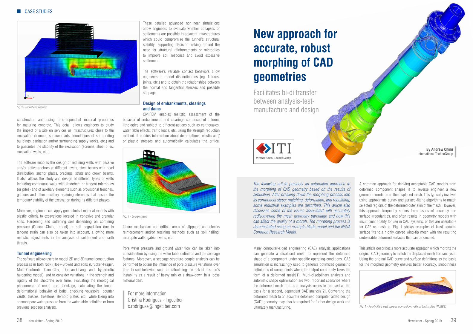
Newsletter - Spring 2019 3938 Newsletter - Spring 2019
CASE STUDIES CASE STUDIES
construction and using time-dependent material properties for maturing concrete. This detail allows engineers to study the impact of a site on services or infrastructures close to the excavation (tunnels, surface roads, foundations of surrounding buildings, sanitation and/or surrounding supply works, etc.) and to guarantee the stability of the excavation (screens, sheet piles, excavation wells, etc.).
The software enables the design of retaining walls with passive and/or active anchors at different levels, steel beams with head distribution, anchor plates, bracings, struts and crown beams. It also allows the study and design of different types of walls including continuous walls with absorbent or tangent micropiles (or piles) and of auxiliary elements such as provisional trenches, gabions and other auxiliary retaining elements that assure the temporary stability of the excavation during its different phases.
Moreover, engineers can apply geotechnical material models with plastic criteria to excavations located in cohesive and granular soils. Hardening and softening soil depending on confining pressure (Duncan-Chang model) or soil degradation due to tangent strain can also be taken into account, allowing more realistic adjustments in the analysis of settlement and earth thrusts.
Tunnel engineeringThe software allows users to model 2D and 3D tunnel construction processes in both rock (Hoek-Brown) and soils (Drucker-Prager, Mohr-Coulomb, Cam-Clay, Duncan-Chang and hyperbolic hardening model), and to consider variations in the strength and rigidity of the shotcrete over time, evaluating the rheological phenomena of creep and shrinkage, calculating the tenso-deformational behavior of bolts, checking voussoirs, counter vaults, trusses, tresillons, Bernold plates, etc., while taking into account pore water pressure from the water table definition or from previous seepage analysis.
These detailed advanced nonlinear simulations allow engineers to evaluate whether collapses or settlements are possible in adjacent infrastructures which could compromise the tunnel’s structural stability, supporting decision-making around the need for structural reinforcements or micropiles to improve soil response and avoid excessive settlement.
The software’s variable contact behaviors allow engineers to model discontinuities (eg. failures, joints, etc.) and to obtain the relationships between the normal and tangential stresses and possible slippage.
Design of embankments, clearings and damsCivilFEM enables realistic assessment of the
behavior of embankments and clearings composed of different lithologies and subject to different actions such as earthquakes, water table effects, traffic loads, etc. using the strength reduction method. It obtains information about deformations, elastic and/or plastic stresses and automatically calculates the critical
failure mechanism and critical areas of slippage, and checks reinforcement and/or retaining methods such as soil nailing, micropile walls, gabion walls, etc.
Pore water pressure and ground water flow can be taken into consideration by using the water table definition and the seepage features. Moreover, a seepage-structure couple analysis can be performed to obtain the influence of pore pressure variations over time to soil behavior, such as calculating the risk of a slope’s instability as a result of heavy rain or a draw-down in a loose material dam.
Fig 3 - Tunnel engineering
Fig. 4 - Embankments
New approach for accurate, robust morphing of CAD geometries Facilitates bi-di transfer between analysis-test- manufacture and design
By Andrew ChinnInternational TechneGroup
The following article presents an automated approach to the morphing of CAD geometry based on the results of simulation. After breaking down the morphing process into its component steps: matching, deformation, and rebuilding, some industrial examples are described. This article also discusses some of the issues associated with accurately rediscovering the mesh geometry parentage and how this can affect the quality of a morph. The morphing process is demonstrated using an example blade model and the NASA Common Research Model.
Many computer-aided engineering (CAE) analysis applications can generate a displaced mesh to represent the deformed shape of a component under specific operating conditions. CAE simulation is increasingly used to generate optimized geometric definitions of components where the output commonly takes the form of a deformed mesh[1]. Multi-disciplinary analysis and automatic shape optimization are two important scenarios where the deformed mesh from one analysis needs to be used as the basis for a second, dependent CAE analysis[2]. Converting the deformed mesh to an accurate deformed computer-aided design (CAD) geometry may also be required for further design work and ultimately manufacturing.
A common approach for deriving acceptable CAD models from deformed component shapes is to reverse engineer a new geometric model from the displaced mesh. This typically involves using approximate curve- and surface-fitting algorithms to match selected regions of the deformed outer skin of the mesh. However, this approach frequently suffers from issues of accuracy and surface irregularities, and often results in geometry models with insufficient fidelity for use in CAD systems, or that are unsuitable for CAE re-meshing. Fig. 1 shows examples of least squares surface fits to a highly curved wing-tip mesh with the resulting undesirable deformed surfaces that can be created.
This article describes a more accurate approach which morphs the original CAD geometry to match the displaced mesh from analysis. Using the original CAD curve and surface definitions as the basis for the morphed geometry ensures better accuracy, smoothness
Fig. 1 - Poorly fitted least squares non-uniform rational basis spline (NURBS)
For more informationCristina Rodriguez - [email protected]

Newsletter - Spring 2019 4140 Newsletter - Spring 2019
CASE STUDIES CASE STUDIES
and continuity. The process also provides significantly better support for sparse deformation data where the traditional least squares fitting approach can struggle to produce usable geometry.
This advanced geometry morphing process supports the import of deformation data from various sources and results in an accurate morphed version of the original CAD geometry. Using this process, it is possible to accurately deform original CAD geometry based upon CAE analysis results.
Mesh-to-CAD matchingBefore the morphing of the CAD geometry can begin, the undeformed mesh needs to be related back to the original CAD geometry and its node parentage needs to be determined to ensure that the nodal displacements from the analysis are applied to the correct areas of the CAD model. Most meshes do not carry the geometry parent information, so this needs to be recovered by matching the mesh to the geometry.
The initial mesh-to-geometry matching algorithm was based on a simple geometric proximity algorithm, projecting nodes onto the CAD model edges to partition the mesh. This method works well for meshes that are perfectly aligned with the geometry, however many meshes are not. A new matching algorithm that can handle a wide range of industrial meshes has been developed to deal with the matching failures caused by the misalignment of the mesh and CAD.
The new matching algorithm makes use of both geometric and topological data to match the mesh to the geometry. The algorithm traces out the edges of the CAD topology onto the mesh; the tracing of an edge onto the mesh is called the edge image. These edge images are used to segment the regions of nodes and elements which are then parented to appropriate faces in the CAD model.
The tracing process does not require the mesh to have nodes exactly on the CAD edges, meaning that the matching is far more robust for misaligned meshes.
Fig. 2 shows a misaligned mesh where the top edge is aligned with the mesh, but the bottom edge is not and crosses several elements. It is possible to find an image of the bottom edge, but it requires a large matching tolerance.
There are cases where no unique images of the edges exist in the mesh, where the mesh topology does not match the topology of the geometry. These cases can broadly be divided into two groups: abstracted edges and virtual topology.
Abstracted edges typically occur in meshes near sharp faces or narrow regions. In these cases, the faces are so narrow that the mesh generator cannot position two distinct nodes on the opposite edges of the face, and so collapses them onto a single node, removing elements from the mesh to avoid making degenerate or
poor-quality elements. Fig. 3 shows an example of an abstracted edge.
The matching algorithm does not require each edge image to be unique for every edge, allowing it to trace out two images from the same edge in the mesh, leading to a full match, even when face regions have been pinched into two distinct regions on the mesh.
Virtual topology (VT) consists of deliberately misaligned mesh spanning several elements and multiple CAD faces. This often occurs in regions of tight curvature or where there are many small CAD faces and the mesh generator cannot mesh the geometry with acceptable element quality. Fig. 4 shows an example of a mesh from a VT region.
In this case, it is not possible to determine the edge images and to match the mesh exactly to the geometry. The nodes within a VT region can still be parented to a unique face, but the elements cannot where they span multiple faces. The lack of element-to-face parenting results means there is insufficient information to morph the geometry, but it does allow for a mesh-to-CAD comparison based on node proximity only. The matching algorithm can discover the extent of the VT regions and identify groups of CAD faces that belong to the VT region. Future enhancements are
Fig. 2 - Misaligned mesh and topology
Fig. 3 - The CAD edges (orange) both use the same element edge (blue) in their edge images
Fig. 4 - Mesh on a virtual topology region
planned to enable nodal deformations to be interpolated from the VT region onto the edges and faces that they cover, thereby enabling morphing.
For morphing to provide valuable benefits in industrial use cases it is required to handle large CAD models with complex geometries and very large meshes. The limiting step in processing very large models is the mesh-to-CAD matching stage. The initial implementation, using just geometric proximity data, limited the matching process to working with a single body, or multiple bodies that did not touch. Coincident meshes from contacting bodies were too complex to untangle, and models containing several bodies could not be morphed as the deformation data could not be applied to the correct surface in touching regions.
Fig. 5 shows an example of a large mesh after CAD geometry/topology matching. The improved matching algorithm achieves greater robustness by making use of the topology of the CAD model and enables the contacting bodies and mesh to be correctly segmented and parented for morphing.
Performance is also significantly improved by the use of the CAD model’s topology. The number of geometrical queries is greatly reduced, allowing the matching algorithm to run in a few seconds, compared to the original basic proximity approach which can require several hours.
The morphing processGeometry morphing can begin once the undeformed mesh has been parented to the original geometry. The deformation vector field is first extracted from two twinned meshes. The first mesh is of the nominal CAD geometry in its undeformed state, and the second mesh is the deformed twin of the same mesh. The second mesh represents the desired deformed shape of the CAD, usually
the result of a simulation. Because the two meshes are twinned, every node on the undeformed mesh is paired to its equivalent on the deformed mesh. The deformation field is calculated from the difference between the two meshes. Each vector in the field will start at a node position on the undeformed mesh and point to the node’s twin on the deformed mesh. Fig. 6 shows an example of a pair of twinned meshes and the corresponding deformation vectors.
The nominal CAD geometry must be defined as a standard CAD boundary representation (BREP). The curves and surfaces are required to be defined using NURBS. Any non-NURBS geometry is converted into a NURBS format prior to the morphing process.
The first step is to morph the vertices of the CAD geometry by a simple translation through the relevant deformation vector derived from the parented nodes.The second step morphs the edges that bound the faces of the CAD geometry. Each CAD edge has a string of matched nodes running along it, each node with its own deformation vector. These deformations are parametrized, and a curve is constructed from them using a least square fitter [3]. The resulting curve can be considered a ‘delta’ curve. The delta curve is then reconciled with the original CAD edge and is finally added to it to produce a new, deformed NURBS edge [4]. Fig. 7 illustrates the process of morphing a simple edge.
The key benefit of deforming using a delta curve is that it preserves any original design intent from the undeformed CAD edge. Fig. 7 shows that the oscillations in the undeformed curve have been carried over to the deformed curve, a benefit that simple fitting to the deformed mesh cannot achieve.
The morphing of the CAD edges reveals why accurately matching the original mesh to the original CAD is so important. If it is unclear how to deform the ends of curves because, for example, the mesh does not align well and was not matched correctly, then the morph will be poor. If a node was matched to the end of the edge but was not exactly on the CAD vertex, then, assuming the deformations are reasonably smooth, the morphing algorithm can
Fig. 5 - Large complex engine example showing matched regions in different colors
Fig. 6 - The deformation vectors between the twinned original and deformed meshes
Fig. 7 - The top edge (green) is meshed by a sparse mesh (blue) and morphed into the bottom edge (green) using the deformed mesh (blue)
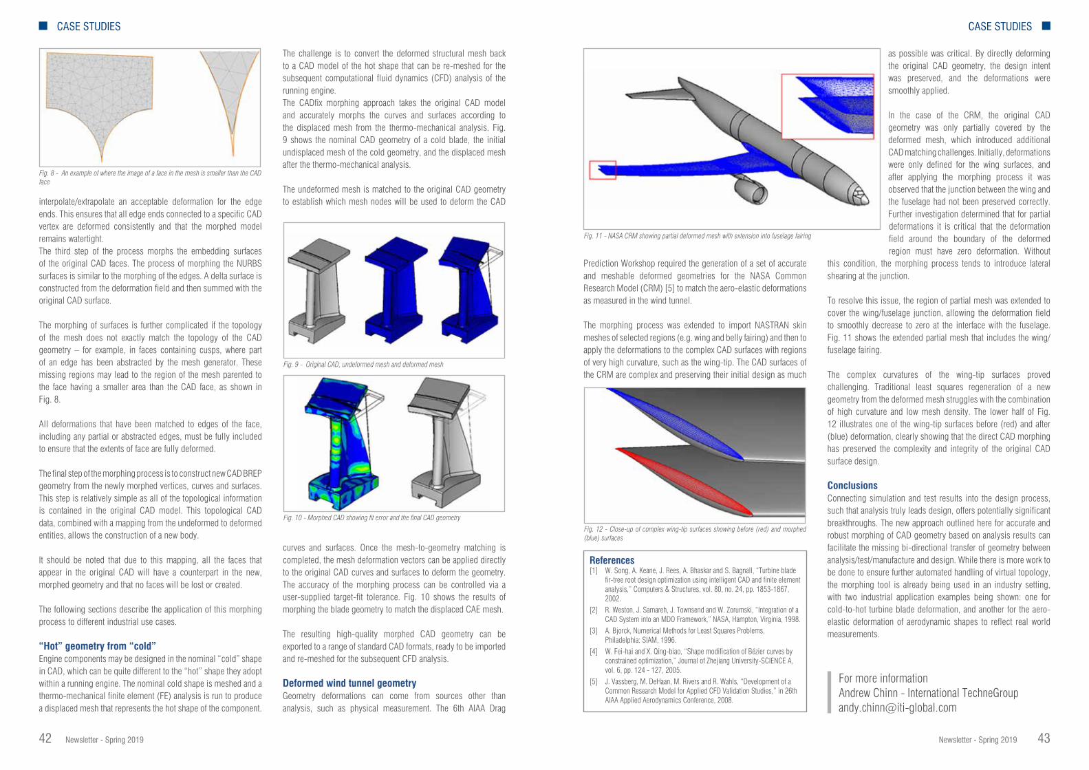
Newsletter - Spring 2019 4342 Newsletter - Spring 2019
CASE STUDIES CASE STUDIES
interpolate/extrapolate an acceptable deformation for the edge ends. This ensures that all edge ends connected to a specific CAD vertex are deformed consistently and that the morphed model remains watertight.The third step of the process morphs the embedding surfaces of the original CAD faces. The process of morphing the NURBS surfaces is similar to the morphing of the edges. A delta surface is constructed from the deformation field and then summed with the original CAD surface.
The morphing of surfaces is further complicated if the topology of the mesh does not exactly match the topology of the CAD geometry – for example, in faces containing cusps, where part of an edge has been abstracted by the mesh generator. These missing regions may lead to the region of the mesh parented to the face having a smaller area than the CAD face, as shown in Fig. 8.
All deformations that have been matched to edges of the face, including any partial or abstracted edges, must be fully included to ensure that the extents of face are fully deformed.
The final step of the morphing process is to construct new CAD BREP geometry from the newly morphed vertices, curves and surfaces. This step is relatively simple as all of the topological information is contained in the original CAD model. This topological CAD data, combined with a mapping from the undeformed to deformed entities, allows the construction of a new body.
It should be noted that due to this mapping, all the faces that appear in the original CAD will have a counterpart in the new, morphed geometry and that no faces will be lost or created.
The following sections describe the application of this morphing process to different industrial use cases.
“Hot” geometry from “cold”Engine components may be designed in the nominal “cold” shape in CAD, which can be quite different to the “hot” shape they adopt within a running engine. The nominal cold shape is meshed and a thermo-mechanical finite element (FE) analysis is run to produce a displaced mesh that represents the hot shape of the component.
The challenge is to convert the deformed structural mesh back to a CAD model of the hot shape that can be re-meshed for the subsequent computational fluid dynamics (CFD) analysis of the running engine.The CADfix morphing approach takes the original CAD model and accurately morphs the curves and surfaces according to the displaced mesh from the thermo-mechanical analysis. Fig. 9 shows the nominal CAD geometry of a cold blade, the initial undisplaced mesh of the cold geometry, and the displaced mesh after the thermo-mechanical analysis.
The undeformed mesh is matched to the original CAD geometry to establish which mesh nodes will be used to deform the CAD
curves and surfaces. Once the mesh-to-geometry matching is completed, the mesh deformation vectors can be applied directly to the original CAD curves and surfaces to deform the geometry. The accuracy of the morphing process can be controlled via a user-supplied target-fit tolerance. Fig. 10 shows the results of morphing the blade geometry to match the displaced CAE mesh.
The resulting high-quality morphed CAD geometry can be exported to a range of standard CAD formats, ready to be imported and re-meshed for the subsequent CFD analysis.
Deformed wind tunnel geometryGeometry deformations can come from sources other than analysis, such as physical measurement. The 6th AIAA Drag
Fig. 8 - An example of where the image of a face in the mesh is smaller than the CAD face
Fig. 9 - Original CAD, undeformed mesh and deformed mesh
Fig. 10 - Morphed CAD showing fit error and the final CAD geometry
Prediction Workshop required the generation of a set of accurate and meshable deformed geometries for the NASA Common Research Model (CRM) [5] to match the aero-elastic deformations as measured in the wind tunnel.
The morphing process was extended to import NASTRAN skin meshes of selected regions (e.g. wing and belly fairing) and then to apply the deformations to the complex CAD surfaces with regions of very high curvature, such as the wing-tip. The CAD surfaces of the CRM are complex and preserving their initial design as much
as possible was critical. By directly deforming the original CAD geometry, the design intent was preserved, and the deformations were smoothly applied.
In the case of the CRM, the original CAD geometry was only partially covered by the deformed mesh, which introduced additional CAD matching challenges. Initially, deformations were only defined for the wing surfaces, and after applying the morphing process it was observed that the junction between the wing and the fuselage had not been preserved correctly. Further investigation determined that for partial deformations it is critical that the deformation field around the boundary of the deformed region must have zero deformation. Without
this condition, the morphing process tends to introduce lateral shearing at the junction.
To resolve this issue, the region of partial mesh was extended to cover the wing/fuselage junction, allowing the deformation field to smoothly decrease to zero at the interface with the fuselage. Fig. 11 shows the extended partial mesh that includes the wing/fuselage fairing.
The complex curvatures of the wing-tip surfaces proved challenging. Traditional least squares regeneration of a new geometry from the deformed mesh struggles with the combination of high curvature and low mesh density. The lower half of Fig. 12 illustrates one of the wing-tip surfaces before (red) and after (blue) deformation, clearly showing that the direct CAD morphing has preserved the complexity and integrity of the original CAD surface design.
ConclusionsConnecting simulation and test results into the design process, such that analysis truly leads design, offers potentially significant breakthroughs. The new approach outlined here for accurate and robust morphing of CAD geometry based on analysis results can facilitate the missing bi-directional transfer of geometry between analysis/test/manufacture and design. While there is more work to be done to ensure further automated handling of virtual topology, the morphing tool is already being used in an industry setting, with two industrial application examples being shown: one for cold-to-hot turbine blade deformation, and another for the aero-elastic deformation of aerodynamic shapes to reflect real world measurements.
References[1] W. Song, A. Keane, J. Rees, A. Bhaskar and S. Bagnall, “Turbine blade
fir-tree root design optimization using intelligent CAD and finite element analysis,” Computers & Structures, vol. 80, no. 24, pp. 1853-1867, 2002.
[2] R. Weston, J. Samareh, J. Townsend and W. Zorumski, “Integration of a CAD System into an MDO Framework,” NASA, Hampton, Virginia, 1998.
[3] A. Bjorck, Numerical Methods for Least Squares Problems, Philadelphia: SIAM, 1996.
[4] W. Fei-hai and X. Qing-biao, “Shape modification of Bézier curves by constrained optimization,” Journal of Zhejiang University-SCIENCE A, vol. 6, pp. 124 - 127, 2005.
[5] J. Vassberg, M. DeHaan, M. Rivers and R. Wahls, “Development of a Common Research Model for Applied CFD Validation Studies,” in 26th AIAA Applied Aerodynamics Conference, 2008.
Fig. 11 - NASA CRM showing partial deformed mesh with extension into fuselage fairing
Fig. 12 - Close-up of complex wing-tip surfaces showing before (red) and morphed (blue) surfaces
For more informationAndrew Chinn - International TechneGroup [email protected]

Newsletter - Spring 2019 4544 Newsletter - Spring 2019
CASE STUDIES CASE STUDIES
less than 900 MPa over the entire profile due to the mechanical limitations of the materials in contact.- The radius of curvature of the cam must be greater than the radius of the roller at all points.
Implementation and resultsFirst-step optimization (MATLAB model)The first step was to generate the curve with MATLAB and obtain the results for jerk, Hertz pressure and force. Fig.3. shows all the variables used for the creation. The Design variables: X=[xb;xe;xf;ye;y’c;y’d;y’e;y’’c;y’’d;y’’e]; For this part, the value of each variable is not very perceptive physically (eg: the jerk at a point) and the range can be very large eg. +/- 106. The mechanism’s response is multimodal, possibly due to the high number of variables.The constraints on the mechanism were also very difficult to handle; only a small range of combinations of variables can adapt to the constraints. The way to find the best solution is to create a Design of Experiments (DOE) of 30 designs and use a MOGA II as the optimization algorithm with 400 generations to explore the domain. This takes two hours, on average, which is quite fast. The second step is to use an adaptive filter sequential quadratic programming (AFSQP) method on the best design found with MOGA II, which allows one to gain 12% on the cost function.
ResultsFig. 4 shows the Hertz pressure. The reduction is 10 MPa, which increases the angular velocity of the cam’s inlet and consequently the productivity of the machine. Fig. 5 shows that the contact force in the second zone increased to 60%, which ensures permanent and reliable contact between the cam and the follower roller. The optimization also leads to continuity of Jerk, which was the third objective of the multi-criteria design optimization.
Second-step optimization (Adam-MATLAB model)The classic dynamic model is not precise enough to estimate the maximum force generated on the mechanism. In reality, other phenomena such as vibration or shock may appear. A good way to estimate this
maximum value is to run a simulation in Adam. To meet the objective of minimizing the maximum force on the mechanism, we must insert Adam into the modeFRONTIER flow, which requires a little adaptation as depicted in Fig.6. The main idea is to use a .cmd file for Adam with the entire mechanism drawn in it and a special part, which is the cam, created on the basis of a spline defined by a point matrix. This point matrix contains all the points of the cam profile. For each design drawing, we have to create a new .cmd file in which the point matrix is modified with the new curve. The .cmd file has a very rigorous structure, so all the modifications must be well oriented to avoid creating errors in the simulation. Then the simulation is run in Adam to obtain the desired data.
The key disadvantage of this approach is that the Adam simulation takes some time to execute so it is useful to limit the time of each simulation in the Adam node. This requires being truly aware of the physical behavior of the mechanism. The algorithm used here is only a MOGA II with 30 DOE and 600 generations.
ResultsIn conclusion, Fig 7 shows that the value of the maximum force has been reduced by 17%, which increases the mechanism’s lifetime by 100 times, on average.
Fig. 6 - Creation algorithm for the cam profile
Fig. 4 - Hertz pressure generated by the previous and optimized laws of motion.
Fig. 5 - Contact force generated by the previous and optimized laws of motion.
Fig. 7 - Flow associated with the Adam view
Fig. 8 - Maximum value of force estimated by Adam for each design
The design of a cam for high-speed production machines with various operating criteria imposes various conflicting objectives that must be addressed to optimize the cam’s performance. This technical case study explains the application of a two-step methodology using the MATLAB and Adam algorithms in the modeFRONTIER software platform. The main objective of the optimization was to reduce the stress inside the cam mechanism, first by optimizing the profile and then considering effects such as shock, vibration and pressure.
Initial problem The design of a cam for high-speed production machines with various operating criteria imposes certain requirements not only on the entire length of the cam profile but on specific zones. These include executing the rise, dwell and return motions of the follower; respecting the positions of the follower roller in the check-points, and ensuring continuity of acceleration at all checkpoints; ensuring permanent contact between the cam and the follower roller; ensuring the minimal contact force in some zones; decreasing the maximum Hertz pressure; maintaining continuity of jerk in acceleration, a minimal pressure angle, a minimal time of return, etc. Clearly, these are conflicting objectives. For this reason, the modeFRONTIER software platform was used for fast process integration and advanced multi-objective optimization.The law of motion associated with the dynamic model is defined as a curve that verifies some checkpoints to control movement. Fig. 2 shows the checkpoints used to generate the curve, which is a polynomial interpolation between the points. The boundary conditions at the second and third order of each point are the variables for deforming the curve and generating the dynamic response.
Methodology The main objective is to reduce the stress in the cam mechanism. There are several factors that can affect it such as Hertz pressure, vibration or shock. Taking this into account, the entire methodology is based on “two-step” optimization.The first step is dedicated to profile optimization and, for this purpose, a dynamic model which excludes some effects like shock and vibration
was used. This part was executed using a MATLAB algorithm which encoded the dynamic response, in addition to another algorithm aimed at generating a law of motion using the pieces of the polynomials function. Then, in the second step, an Adam optimization algorithm was used for the other phenomena. The mechanism was created in Adam with appropriate contact parameters between the cam and the follower and using values obtained from real tests on the machine.
The objectives and constraints of the optimizationsThe MATLAB optimization:There were three objectives related to the zones in which they were located. n The maximum Hertz pressure, in the first zone of the curve for t
∈ [0; 0.4s] (Fig. 5) had to be minimized in order to increase the cam’s inlet rotation velocity and consequently the productivity of the machine.
n The minimum contact force between the cam and the roller, in the second zone of the curve for t ∈ [0.04s; 0.06s] had to be maximized to ensure permanent contact. Observations had shown that a loss of contact was possible in this zone.
n The Jerk, in the third zone of the curve for t ∈ [0.09s; 0.18s], where constraints were rather weak, had to be minimized to reduce vibration.
The Adam optimization:n The maximum value of the force between the cam and the
follower had to be minimized. There are four constraints defined for the reliable operation of a cam mechanism.- The maximum displacement |y|<58 mm, due to the permissible extension of the spring.
n F >50 N over the entire profile to ensure permanent contact between the cam and the follower roller.- Hertz Pressure must be
Optimizing a cam mechanism using Adam and MATLAB By Léo Moussafir1 and Vito Primavera2
1. Sidel GROUP - 2. EnginSoft
Fig. 1 - Cam mechanism with spring, assuming contact between the cam and the follower roller.
Fig. 2 - The cam mechanism’s current law of motion must be optimized.
For more informationVito Primavera - [email protected]

Newsletter - Spring 2019 4746 Newsletter - Spring 2019
CASE STUDIES CASE STUDIES
technology (Figures 1 and 2) that can transfer 3 kW between two coils with an efficiency higher than 96.5%. The interval of the two coils is 100-160 mm, and the frequency of the AC power is 81-90 kHz.
This technology will enable EV users to charge the battery without connecting any cables. The technology is based on two coils: one coil built into roads, parking spaces, or garages and the other fitted to the underbody of the car. A coil case with magnetic and conductive properties produces an eddy current and decreases the power efficiency.
Therefore, it is necessary to apply non-magnetic, nonconductive plastic or ceramic materials as the coil case material. However, their materials strength is generally low. Furthermore, the coil case must protect the coils, ferrite, and electric parts (Figure 3).According to the UL standard, a vehicle overdrive test must be performed on the power transmission coil such that even if a vehicle rides on the power transmission coil case, it should not be damaged. The load of the car tire was assumed to be about 5 kN. Glass-fiber-reinforced plastic was selected as the material of the coil case. It is very important to estimate the strength of a coil case made of the glass-fiber-reinforced plastic while designing. Consequently, the Young’s moduli of the glass-fiber-reinforced plastics were estimated by applying the homogenization method
to regular material composition and the value obtained by averaging the elastic modulus by laminating theory to irregular material composition.
The prototype of a coil case made of the glass-fiber-reinforced plastic was designed and fabricated. In addition, the Young’s moduli of the calculation and the prototype were compared. As a consideration, when the prototype was examined, air gaps were observed in the laminated part of the composite material. Therefore, the scales were defined for the analysis. First, the microscale was defined as a scale that can express the characteristics of glass fibers in micrometer order such as the irregularity of glass mat and the regularity of glass cloth.
Next, the macroscale was defined as a scale that can express the characteristics of the composite material in millimeter order such as the regular placement of resin, glass mat, and glass cloth. Finally, the mesoscale was defined as a micrometer to millimeter order unit to measure the air gap in the laminated part of the matrix and the glass fiber. The material irregularity due to the material process could be expressed by mesoscale. A schematic of the defined model is shown in Figure 4.
By comparing these three scales and the glass-fiberreinforced plastic while considering regularity and irregularity, the calculation result was compared with the experimental result.
Numerical Computation Technique to Examine Glass Fiber Mat and Cloth Reinforcement of Glass-Fiber-Reinforced Plastic
TDK is developing a wireless power transfer technology for electric vehicles (EV) that is based on two coils: one built into roads, parking spaces, or garages and the other fitted to the underbody of the car.
One of these coils is the power transmission coil, and the other is the receiving coil. The receiving coil receives the magnetic field generated by the power transmission coil. Furthermore, the rectifier rectifies the alternating current to direct current. A coil case with magnetic and conductive properties produces an eddy current and decreases the power efficiency. Therefore, non-magnetic and non-conductive materials must be adopted in the design of the coil case. Furthermore, the coil case must protect the coil, ferrite cores, and the electronic component array.
According to the Underwriters Laboratories Inc. (UL) standard, a vehicle overdrive test must be performed on the power transmission coil such that even if a vehicle rides on the power transmission coil case, it should not be damaged. In addition, a prototype of the power transmission coil case made of glassfiber-
reinforced plastic was created. During the glass-fiberreinforced plastic molding process, the glass fiber bundle slipped and air gaps were formed. We decided to consider the scale of three patterns: micro, macro, and mesoscale. After considering the three scales, the experimental results and calculated results matched with high accuracy.
1. IntroductionRecently, electric vehicles (EV) have attracted considerable attention because they can prevent global warming and save natural resources such as oil.
They can also reduce carbon dioxide by using renewable energy, including solar and wind energy.
The government predicts that the number of EV and plug-in hybrid EV (PHEV) will increase in the near future [1]. As the number of EV and PHEV vehicles increases, the number of chargers to be installed will also increase. The government has predicted the installation of 2 million normal chargers and 5 million quick chargers by 2020. TDK has developed a wireless power transfer
Fig. 2 - Components of the system
Fig. 3 - Structure of the coil case
Fig. 4 - Schematic of the defined model
Fig. 5 - Prototype coil case
Fig. 6 - Glass fiber mat Fig. 7 - Glass fiber cloth
Fig. 8 - Glass fiber laminating structure of the coil
By Masayuki Sugasawa, Masayuki Kobayashi, and Takuya MurashigeTechnology & Intellectual Property HQ, TDK Corporation
Fig. 1 - Wireless Power Transfer System developed by TDK Corporation
J. Fiber Sci. Technol., 74(5), 109-116 (2018) doi 10.2115/fiberst.2018-0017©2018 The Society of Fiber Science and Technology, Japan
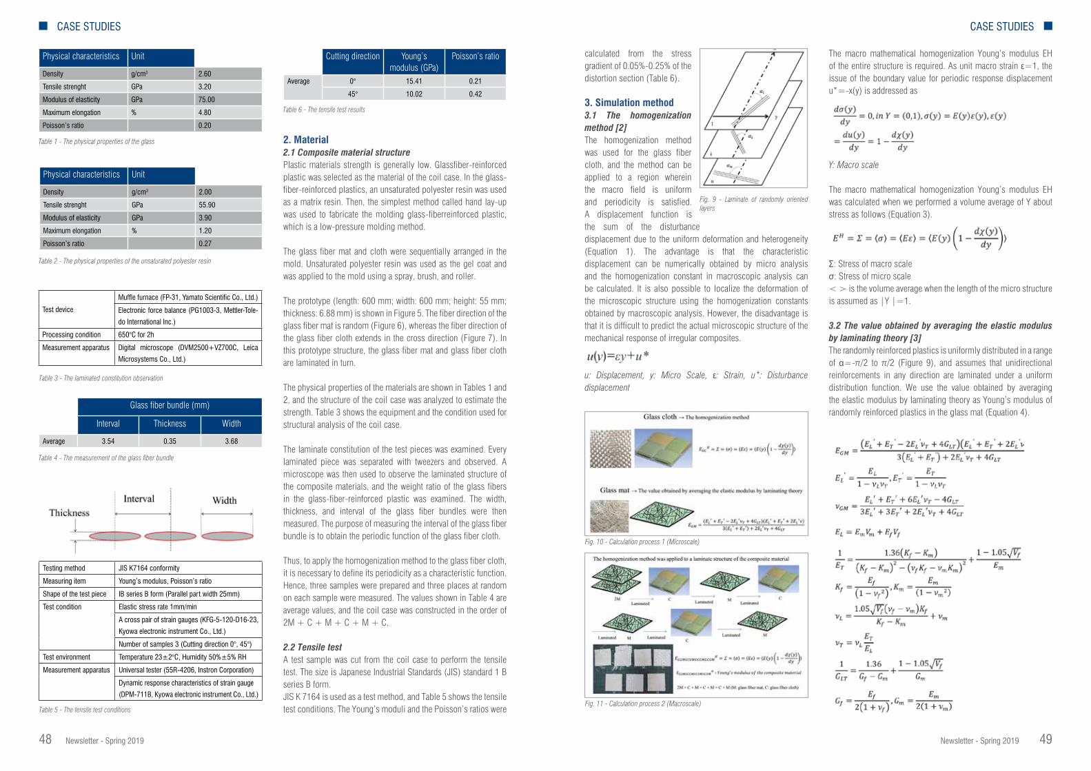
Newsletter - Spring 2019 4948 Newsletter - Spring 2019
CASE STUDIES CASE STUDIES
calculated from the stress gradient of 0.05%-0.25% of the distortion section (Table 6).
3. Simulation method3.1 The homogenization method [2]The homogenization method was used for the glass fiber cloth, and the method can be applied to a region wherein the macro field is uniform and periodicity is satisfied. A displacement function is the sum of the disturbance displacement due to the uniform deformation and heterogeneity (Equation 1). The advantage is that the characteristic displacement can be numerically obtained by micro analysis and the homogenization constant in macroscopic analysis can be calculated. It is also possible to localize the deformation of the microscopic structure using the homogenization constants obtained by macroscopic analysis. However, the disadvantage is that it is difficult to predict the actual microscopic structure of the mechanical response of irregular composites.
u: Displacement, y: Micro Scale, ε: Strain, u*: Disturbance displacement
The macro mathematical homogenization Young’s modulus EH of the entire structure is required. As unit macro strain ε=1, the issue of the boundary value for periodic response displacement u*=-x(y) is addressed as
Y: Macro scale
The macro mathematical homogenization Young’s modulus EH was calculated when we performed a volume average of Y about stress as follows (Equation 3).
Σ: Stress of macro scaleσ: Stress of micro scale< > is the volume average when the length of the micro structure is assumed as |Y |=1.
3.2 The value obtained by averaging the elastic modulus by laminating theory [3]The randomly reinforced plastics is uniformly distributed in a range of α=-π/2 to π/2 (Figure 9), and assumes that unidirectional reinforcements in any direction are laminated under a uniform distribution function. We use the value obtained by averaging the elastic modulus by laminating theory as Young’s modulus of randomly reinforced plastics in the glass mat (Equation 4).
2. Material2.1 Composite material structurePlastic materials strength is generally low. Glassfiber-reinforced plastic was selected as the material of the coil case. In the glass-fiber-reinforced plastics, an unsaturated polyester resin was used as a matrix resin. Then, the simplest method called hand lay-up was used to fabricate the molding glass-fiberreinforced plastic, which is a low-pressure molding method.
The glass fiber mat and cloth were sequentially arranged in the mold. Unsaturated polyester resin was used as the gel coat and was applied to the mold using a spray, brush, and roller.
The prototype (length: 600 mm; width: 600 mm; height: 55 mm; thickness: 6.88 mm) is shown in Figure 5. The fiber direction of the glass fiber mat is random (Figure 6), whereas the fiber direction of the glass fiber cloth extends in the cross direction (Figure 7). In this prototype structure, the glass fiber mat and glass fiber cloth are laminated in turn.
The physical properties of the materials are shown in Tables 1 and 2, and the structure of the coil case was analyzed to estimate the strength. Table 3 shows the equipment and the condition used for structural analysis of the coil case.
The laminate constitution of the test pieces was examined. Every laminated piece was separated with tweezers and observed. A microscope was then used to observe the laminated structure of the composite materials, and the weight ratio of the glass fibers in the glass-fiber-reinforced plastic was examined. The width, thickness, and interval of the glass fiber bundles were then measured. The purpose of measuring the interval of the glass fiber bundle is to obtain the periodic function of the glass fiber cloth.
Thus, to apply the homogenization method to the glass fiber cloth, it is necessary to define its periodicity as a characteristic function. Hence, three samples were prepared and three places at random on each sample were measured. The values shown in Table 4 are average values, and the coil case was constructed in the order of 2M + C + M + C + M + C.
2.2 Tensile testA test sample was cut from the coil case to perform the tensile test. The size is Japanese Industrial Standards (JIS) standard 1 B series B form.JIS K 7164 is used as a test method, and Table 5 shows the tensile test conditions. The Young’s moduli and the Poisson’s ratios were
Cutting direction Young’smodulus (GPa)
Poisson’s ratio
Average 0° 15.41 0.21
45° 10.02 0.42
Physical characteristics Unit
Density g/cm3 2.60
Tensile strenght GPa 3.20
Modulus of elasticity GPa 75.00
Maximum elongation % 4.80
Poisson’s ratio 0.20
Physical characteristics Unit
Density g/cm3 2.00
Tensile strenght GPa 55.90
Modulus of elasticity GPa 3.90
Maximum elongation % 1.20
Poisson’s ratio 0.27
Test device
Muffle furnace (FP-31, Yamato Scientific Co., Ltd.)
Electronic force balance (PG1003-3, Mettler-Tole-
do International Inc.)
Processing condition 650°C for 2h
Measurement apparatus Digital microscope (DVM2500+VZ700C, Leica
Microsystems Co., Ltd.)
Glass fiber bundle (mm)
Interval Thickness Width
Average 3.54 0.35 3.68
Testing method JIS K7164 conformity
Measuring item Young’s modulus, Poisson’s ratio
Shape of the test piece IB series B form (Parallel part width 25mm)
Test condition Elastic stress rate 1mm/min
A cross pair of strain gauges (KFG-5-120-D16-23,
Kyowa electronic instrument Co., Ltd.)
Number of samples 3 (Cutting direction 0°, 45°)
Test environment Temperature 23±2°C, Humidity 50%±5% RH
Measurement apparatus Universal tester (55R-4206, Instron Corporation)
Dynamic response characteristics of strain gauge
(DPM-711B, Kyowa electronic instrument Co., Ltd.)
Table 1 - The physical properties of the glass
Table 2 - The physical properties of the unsaturated polyester resin
Table 3 - The laminated constitution observation
Table 4 - The measurement of the glass fiber bundle
Table 5 - The tensile test conditions
Table 6 - The tensile test results
Fig. 9 - Laminate of randomly oriented layers
Fig. 10 - Calculation process 1 (Microscale)
Fig. 11 - Calculation process 2 (Macroscale)

Newsletter - Spring 2019 5150 Newsletter - Spring 2019
CASE STUDIES CASE STUDIES
EGM: Young’s modulus of randomly reinforced plastics (Glass mat)VGM: P oisson’sratio of randomly reinforced plastics (Glassmat)EL: Y oung’s modulus of fiber horizontal directionET: Y oung’s modulus of fiber vertical directionEf: Young’s modulus of fiberEm: Young’s modulus of matrixVf: Fiber contentVm: Matrix contentKf: Bulk modulus of fiberKm: Bulk modulus of matrixVf: Poisson’s ratio of fiberVm: Poisson’s ratio of matrixVL: Poisson’s ratio of fiber horizontal directionVT: Poisson’s ratio of fiber vertical directionGLT: Elastic shear modulus of fiber horizontal directionGf: Elastic shear modulus of fiberGm: Elastic shear modulus of matrix
4. Simulation techniqueThe Young’s modulus for the composite material was calculated using the homogenization method and the value obtained by averaging the elastic modulus by laminating theory. The coil case was composed of 2M + C + M + C + M + C + M (M: glass fiber mat, C: glass fiber cloth) using an unsaturated polyester resin as a matrix. In the estimation of Young’s modulus in the fiber direction, the homogenization method was applied to the glass fiber cloth, the value obtained by averaging the elastic modulus by laminating theory was applied to glass fiber mat, and the homogenization method was applied to a laminate structure of the composite material. The explanation contents are shown in Figure 10 and 11. Furthermore, Multiscale. Sim made by Cybernet Systems Co., Ltd. was used for the homogenization method. This software is a micro and macro scale analyzable simulation based on the homogenization method [4-7] when the composite material is periodic. In other words, it calculates the macroscale material constants by homogenizing the microscale material constants.In addition, it can perform micro scale detailed analysis by localizing the macroscale part, and the characteristic to be considered in the macroscale governing equation is the body force (The force proportional to the volume and mass of the substance).The characteristic to be considered in the microscale governing equations [8, 9] is the disturbance displacement. In this analysis, homogenization analysis was mainly performed as the numerical material test. The displacement of the micro structure is the sum of the uniform displacement and the periodic disturbance displacement due to nonhomogeneity. Lastly, the Young’s modulus of the homogenized unit cell was obtained from the analysis result by integrating the stress of the unit cell and taking the volume average of the unit cell [10-12].
5. DiscussionA test sample (width: 40 mm; length: 40 mm; thickness: 6.8 mm) was cut from the coil case, and its cross-section was observed using a digital microscope (at 35 × magnification). Figure 12
shows a photograph of the section observation, and the matrix thickness of the outermost layer of the cut surface was about 200 μm. As a result of this observation, some air gaps were found in the laminated structure of the glass mat, the glass cloth, and the matrix. The cause of some air gaps were presumed to be the molding method. The simplest method called hand lay-up was used for molding the glass-fiber- reinforced plastic.This method is a low-pressure molding method, and some air gaps were formed in the laminated structure due to insufficient pressurization during heat curing. Moreover, some air gap size was measured with a digital microscope, and the volume ratio of some air gaps in the composite material was 30%.
Fig. 12 - Test sample section observation
Fig. 13 - Additional calculation process (Mesoscale)
Fig. 14 - 1B series B form of the composite material
X-Y directionYoung’s modulus
(GPa)
Experiment(GPa)
Simulation(GPa)
Error (%)
0° 15.41 15.92 3.28
45° 10.02 10.39 3.74
Table 7 - The results of tensile test in the experiment and simulation
The mesoscale was defined as a micrometer to millimeter order unit such that the air gap in the laminated part of the matrix and the glass fiber, as well as the material irregularity, was expressed by the manufacturing process on this scale. Conventionally, some methods based on the equivalent inclusion method [13] and the Weibull probability distribution method [14] have been studied for calculating the physical properties of a composite material containing probabilistically certain material.However, as a result of this observation, some air gaps were confirmed to be scattered along the glass fiber lamination.Therefore, the experimental result was compared with the calculation result by using the rule of mixture for estimating the Young’s modulus of the composite material in the fiber direction.The Young’s modulus calculation procedure of the composite material is shown in Figure 13 based on the previous discussion.
6. ResultThe Young’s moduli in the direction of the glass fiber were compared in the experimental and the numerical material test. The experimental result was the average value of the number of samples n = 3. As shown in Table 5, the sample shape was a 1 B series B form shape according to JIS K 7164 test method. This shape was also imputed to the tensile test simulation, and the laminate structure of 2 M + C + M + C + M + C + M (M: glass fiber mat, C: glass fiber cloth) was inputted using the unsaturated
polyester resin as a matrix. Furthermore, the numerical material testing function of Multiscale.sim was used to simulate the tensile test (Figure 14). Finally, the rule of mixture was applied to the numerical material simulation result to consider the volume ratio of some air gaps, and the difference between the experimental and simulation result was about 4% (Table 7).To summarize, the following procedure was performed:n The homogenization method was applied to the glass fiber
cloth, and the value obtained by averaging the elastic modulus by laminating theory was applied to the glass fiber mat on the microscale.
n The homogenization method was applied to the laminate structure of the glass fiber cloth, the glass fiber mat, and the matrix resin on the macroscale.
n As a result of the prototype observation, some air gaps were scattered along the glass fiber lamination. Therefore, the volume ratios of the air gaps and the composite material were divided into the high and low glass fiber densities, and the Young’s modulus of the composite material in the fiber direction was estimated using the rule of mixture.
Moreover, as a result of about 4% error, the following was considered: First, the cross-section observation image of the prototype in digital image was obtained. The acquired image was expressed in density with 8 bit gradation. At this time, the gray level of the image was selected as black or white depending on the threshold value. Lastly, the imagevolume ratio of the air gap in the composite material changed based on the threshold value. Therefore, it seems that about 4% error occurred in the calculation and the experiment result depending on how to decide the threshold value.
7. ConclusionThe material properties for the micro, macro, and mesoscale were evaluated to estimate the Young’s moduli of the glass-fiber-reinforced plastics. The material irregularities by the manufacturing process were then measured. Consequently, the material irregularities and some air gaps in the mesoscale were modeled and highly precise analytical data were obtained. An effective method for trial verification was also obtained, and this method will be applied to prototype wireless power transmission coil cases for EVs in the future studies.
AcknowledgmentsThe authors would like to thank Mr.Yamamoto, Mr.Sato, Mr.Yano, and Mr.Manaka of Cybernet Systems Co., Ltd. for their advice on the simulation.
Note: The mentioned software, Multiscale.Sim, is now called CMAS.
For more informationAlessandro Mellone - [email protected]
References[1] Electric Vehicle, Advanced Technology and ITS Promotion Office and
Automobile Division, Manufacturing Industries Bureau, “The Road Map for EVs and PHVs toward the Dissemination of Electric Vehicles and Plug-in Hybrid Vehicles”, Ministry of Economy, Trade and Industry, http://www.meti.go.jp/english/ press/2016/0323_01. html, (accessed 2017-06-26).
[2] K. Terada, N. Kikuchi, “ Introduction to homogenization method” (in Japanese), Maruzen publishing, Tokyo, p.13 (2003).
[3] M. Uemura, M. Iyama, Y. Yamaguchi, Bulletin of the Institute of Space and Aeronautical Science, University of Tokyo, 12, 815 (1976).
[4] G. Papanicolau, A. Bensoussan, JL. Lions, “Asymptotic Analysis for Periodic Structures, Vol.5”, Elsevier, Amsterdam, p.12 (1978).
[5] E. Sanchez Palencia, “Non Homogeneous Media and Vibration Theory”, Springer-Verlag, Heidelberg, p.24 (1980).
[6] J. L. Lions, “Some methods in mathematical analysis of systems and their control”, Science Press, Beijing, (1981).
[7] K. Terada, J. Kato, N. Hirayama, T. Inugai, K. Yamamoto, Comput. Mech., 52(5), 1199 (2013).
[8] K. Terada, N. Kikuchi, Comput. Methods Appl. Mech. Eng., 190, (40-41), 5427 (2001).
[9] K. Terada, T. Inugai, N. Hirayama, Trans. Jpn. Soc. Mech. Eng. A, 74(744), 1084 (2008).
[10] K. Terada, T. Inugai, H. Hamana, A. Miyori, N. Hirayama, Transactions of JSCES, 2008, 20080024 (2008).
[11] K. Terada, N. Hirayama, K. Yamamoto, J. Kato, T. Kyoya, S. Matsubara, Y. Arakawa, Y. Ueno, N. Miyanaga, Adv. Compos. Mater., 23(5-6), 421 (2014).
[12] K. Terada, N. Hirayama, K. Yamamoto, S. Matsubara, Transactions of JSCES, 2015, 20150001 (2015).
[13] K. Thogo, K. Kawahara, Y. Sugiyama, Trans. Jpn. Soc. Mech. Eng. A, 67(661), 1493 (2001).
[14] T. Okabe, K Ishii, M. Nishikawa, N. Takeda, J. Jpn. Soc. Comps. Mater., 33(6), 205 (2007).

Newsletter - Spring 2019 5352 Newsletter - Spring 2019
CASE STUDIES CASE STUDIES
The following article is the final part of a three-part series. This first part described Advanced Integrated Engineering Solutions’ system analysis framework, the second part described the abstraction techniques the company uses to aid large system analyses. This third part introduces the company’s Tribology solutions (or joints) for machine design.
The bearing design process at AIES LtdThe analysis of sliding bearings for many applications are shown below in Figure 1. Sliding bearings are found in internal combustion (IC) engines, turbo machines, mechanisms, gears, rolling element bearings (REBs) etc. The analyses are used for steady state, dynamic, instability, and stiffness and damping coefficients. AIES Ltd has analytical, numerical, and multi-body dynamics (MBD) solutions, such as short bear approximation
(SBA), short and long bearing approximation (SALBA), rigid hydro dynamics (RHD), elasto hydro dynamics (EHD), thermo- elasto hydro dynamics (TEHD) and elasto hydrodynamic lubrication (EHL). It also has many different MB and dynamic time marching solutions such as Newmark Beta, Bulirsch Stoer and Rung Kutta Cash Karp (RKCK). Note that AIES’s analytical solutions also work with its dynamic time marching methods.
Typical bearing applicationsFigure 2 below shows two typical bearing applications. The left-hand side (LHS) shows a hydrodynamic journal bearing that might be used in a number of machines, and that would
normally run with a C/R ratio of 0.001, 1 thousand per inch of diameter. C = Rbearing – Rjournal and eccentricity e = O – O’ and e/C = eccentricity ratio. The right-hand side (RHS) shows a typical thrust bearing, termed a hydrodynamic thrust bearing, that normally runs with a (hmax-hmin)/l of 1/10,000. This is equivalent to 0.5”, or 12.7mm over the length of a football pitch.
Oil film lubrication in sliding bearingsFigure 3 below shows the close-up of two Tribological surfaces passing over each other, separated by an oil film. The oil film reduces wear by supporting the two separated surfaces. It can be seen on the RHS (top) boundary lubrication and RHS (bottom) mixed and hydrodynamic lubrication. Note that under some initial boundary lubrication regimes, hydrodynamic can arise due to the thermal arching (deformation) of one of the surfaces.
Figure 4 below shows the three major lubrication regimes used in fluid-film lubrication. It shows that for hydrodynamic lubrication, the asperities of each surface are fully separated. However, for mixed lubrication, the asperities can be just touching or fully separated. The boundary lubrication regime
Tribology solutions for fluid lubricated bearings in machines By Dr Ian McLuckie
Managing and Technology Director for Advanced Integrated Engineering Solutions
PART 3
Fig. 1 - AIES Ltd’s Tribology applications for machines
Fig. 2 - Typical bearing applications.
Fig. 3 - Definition of sliding bearing lubrication regimes and lambda ratios
shows the asperities are always in contact, and lubrication is based on HP or EP additives and wear taking place. The Stribeck curve below in Figure 4 shows the different regimes of lubrication.There are many Tribology interfaces in typical machines such as IC engines, electric motors/generators, gas turbines, pumps, and turbo chargers. AIES Ltd’s program’s structure allows multiple simultaneous solutions e.g. full floating bearings (FFB), and crankshafts. Its Tribology solutions are utilized in its systems software EngineDesigner and SystemDeveloper. The results in Figure 5 show how AIES Ltd can predict component and subsystem regimes of lubrication and frictional losses.
The Reynolds equation – the basis of all oil film lubrication solutionsThe Reynolds equation:
• Developed to explain Beauchamp Tower’s experiments (1883). LHS of figure 6 below
• Invented by Reynolds (1886) to try and understand Beauchamp Tower’s tests.
• 2D partial differential equation above (derived from Navier Stokes equations)
• Solved analytically with simplifying assumptions, including LBA, SBA and SALBA. See figure 6.
• Can be solved numerically by finite-difference (FD) methods for general cases, such as RHD, EHD and TEHD. See figure 6.
Analytical solutions of the Reynolds equation – for a rigid shaft and housing
a) Long bearing approximation (LBA) Due to Sommerfeld (1904), assumes constant axial pressure
distribution and is only suitable for very long bearings.b) Short bearing approximation (SBA) (rotating and
stationary) Due to Ocvirk and Dubois (1965), assumes axial parabolic
pressure distribution. Only suitable for low L/D ratios and small eccentricity ratios (low loads). AIES Ltd has added squeeze velocity terms (AIES Ltd IPR)
c) Short and long bearing approximation (SALBA) (rotating and stationary)
Due to Reason and Narang (1982); a combined SBA and LBA solution, good for all L/D ratios and eccentricity ratios. AIES Ltd has added squeeze velocity terms (AIES Ltd IPR). SALBA is the company’s main analytical solution.
Numerical solutions techniques rotating and stationaryThe numerical meshing method for RHD has a regular grid and general shapes of oil film and includes deformation. The Reynolds equation is transformed into FD form. It allows any boundary conditions including slots and oil holes. The equations of motion (MBD) are solved using the Newmark Beta, Bulirsch Stoer, and RKCK methods. The oil film solution is by an iterative over-relaxation method (Southwell, 1946).
Fig. 4 - Stribeck curve showing lubrication regimes and lambda ratios.
Fig. 5 - Friction regimes predicted by AIES Ltd Tribology software. The different regimes of lubrication captured by the various sub-systems of typical engines can be seen.
Fig. 6 - Beauchamp Towers experiments/tests (LHS) and the difference between SALBA and RHD solutions
Fig. 7 - The three analytical equations that estimate Reynolds bearing behavior. SALBA is very good.
Fig. 8 - FD grid and Reynolds equations showing the oil film shape for SBA/SALBA, RHD, EHD and TEHD

Newsletter - Spring 2019 5554 Newsletter - Spring 2019
CASE STUDIES CASE STUDIES
Numerical solution examplesThese numerical solutions are known at AIES Ltd as a) rigid hydrodynamics (RHD) FD for oil film shape including manufactured profile and oil holes and slots (in journal or bearing), b) elasto hydrodynamics (EHD) as RHD plus deformation due to oil film pressure, and c) thermo-elasto hydrodynamics (TEHD) as EHD but with additional deformation due to thermal loading. RHD solution. Solves equations of motion at the surface of the bearing structure simultaneously with solving the Reynolds equation.
EHD solution. Solves equations of motion at the surface of the bearing structure simultaneously with solving the Reynolds equation. Finite Element mass and stiffness matrices are reduced to the surface nodes. The program includes multiplying factors on stiffness and mass (check stiffness matrix). The plotted orbits show the EHD solution (red) progressively homing in on the RHD solution (blue) as the stiffness is increased to 1000x. This check shows that EHD is working correctly by converging on RHD.
Typical results – analytical vs numerical. Figure 11 shows comparisons of steady state and dynamic simulations: LHS and middle – SBA, LBA, SALBA (analytical solutions) with RHD for a circular bearing without an oil hole. SALBA is almost as accurate as RHD; RHS – comparison of SBA, SALBA and RHD for a dynamically loaded big end. SALBA and RHD cannot be easily separated. Since SBA overestimates film thickness, AIES does not use it very often.
Various bearing simulation examples for rotor dynamics, instability and EHLMajor stiffness and damping coefficients. Stiffness and damping coefficients are used to represent the physical oil film as a set of 4 stiffness and 4 damping coefficients. These are used in rotor dynamic codes, such as ANSYS for example. In figure 12’s comparisons of stiffness coefficients for SBA, SALBA and RHD, it can be seen that SALBA (analytical) follows
RHD (numerical) very closely for all 4 stiffness coefficients. SBA over-estimates the stiffness coefficients for each case, unless at
very low eccentricity (low load). The same relationship is also true for damping coefficients. SALBA is a good approximation for derivation of plain bearing coefficients.
Bearing instability and how to control with gross unbalance. Bearing instability is sometimes overlooked in the design process. Half-frequency whirl is analogous to the oil film stalling, meaning the Coriolis forces exactly match the gravitational or bearing load such that there is no additional load carrying capacity left in the bearing. A speed sweep was carried out up and down the speed
Fig. 9 - Real crankshaft bearing with RHD and EHD bearing simulations
Fig. 10 - EHD results for a typical big end bearing simulation
Fig. 11 - Steady state simulations between SBA, SALBA and RHD (LHS). Dynamic simulations by SBA, SALBA and RHD (RHS).
Fig. 12 - Comparisons of 4 stiffness components – note how the red and yellow lines coincide for SALBA and RHD.
Fig. 13 - Instability (LHS). Stable due to controlled gross unbalance (RHS).
range with the speed-dependent loads to search for the jump phenomena shown in Figure 13 below. Gross unbalance is a good means of controlling instability onset, plus one can use special bearing forms as well.
EHL – lubrication examples. Elasto hydrodynamic lubrication (EHL), used for non-conforming contacts where the contact zone is close to being a line or ellipse, such as gear tooth contacts, cam, and follower and rolling element bearings. Based on the work of BLOK and is a scuffing thermal mechanical model. Includes the effects of pressure-viscosity and the generation of a flash temperature. Figure 14 shows the results for a cam-tappet (LHS – RHS below). The contact patch on the tappet surface (blue) is the likely wear area. The oil film temperature exceeds published oil flash temperature and the minimum oil film thickness is well below three times the composite surface roughness.
Other bearing solutions – piston and linerSolutions for RHD, EHD, TEHD, and the equations of motion are applicable to many Tribology systems. These plots are animated over the cycle. AIES’s software is also applied to tappets, piston rings and pistons (shown here). The top image shows the pressure distribution on the cylinder liner and piston pin orbit. The bottom image shows the piston pressure with the cylinder liner and piston secondary motion.
Cavitation damageAIES Ltd likes to provide results that engineers can use, in addition to plots of orbits, maximum oil film pressure, and minimum oil film thickness, as well as maps of derived results, e.g. cavitation damage parameter accumulated over the operating cycle. The photo of the cavitation damage is taken from Forstner and Struwe (2004). AIES Ltd’s solutions can predict the same patterns of damage, the same effect of changing clearance, rate of pressure increase, etc.
ConclusionsAIES has a lot of bearing solutions for all manner of machines and systems. The solutions can be analytical (SBA, SALBA and EHL) for the early stages of the design, or numerical (RHD, EHD and TEHD) for the latter stages, or even for trouble shooting. These models have been validated against published data, actual machine tests and rig testing.
AIES solutions can predict the location of cavitation damage and simulate whole engines and machine performance. They can abstract fluid films to springs and dampers via their stiffness and damping coefficients and they can predict the onset of instability in bearing systems.
They can simulate sliding, rotating and stationary bearings for pistons, journals and squeeze film dampers respectively, as well as housing elasticity and thermal effects in bearings.
For more information about Tribology, Tribo-Dynamics and machine design, please contact AIES at www.aiesl.co.uk
Fig. 14 - EHL lubrication of a cam and tappet.
Fig. 15 - Piston and liner simulations showing animated pressures, secondary motion and piston trajectory plot.
Fig. 16 - Comparisons of predicted areas of cavitation erosion damage with real bearing damage
For more informationIan McLuckie - AIES [email protected]

Newsletter - Spring 2019 5756 Newsletter - Spring 2019
CASE STUDIES
ANSYS nCode DesignLife is the world’s leading finite element method (FEM)-based fatigue calculation software. While analysts can use it as a standalone tool, it is perfectly integrated into ANSYS Workbench. It allows the user to quickly create complex load histories (duty cycles) either by importing external signals, or by creating and processing internal signals.
The software supports all fatigue calculation methods, including:n stress-lifen strain-lifen spot weldsn seam weldsn vibration fatiguen accelerated testingn virtual strain gauges correlationn high temperature fatiguen crack propagation
Here we discuss the auto elimination method, which is integrated into ANSYS nCode DesignLife, and which allows the user to reduce the calculation time of a fatigue analysis through an automatic procedure that is extremely fast to set up and launch. The method uses a prior selection of the most critical nodes (done by means of a quick assessment of the damage) to carry out the detailed fatigue analysis.
This drastically reduces the total number of nodes to be analysed while ensuring that all the most critical points of the component are calculated in detail. To illustrate the method, we have used the component shown in Figure 1, meshed with 1,700,000 nodes.The component is subject to two independent external loads, shown in Fig. 2: the first signal is applied to one arm of the component, the second signal to the other arm. This independence generates a non-proportional multi-axial condition, which can be calculated using the critical plane criterion. The fatigue analyses are only performed on the skin surface,
which significantly reduces the total number of nodes to be calculated from 1,700,000 to 116,240. In addition, to use the auto elimination method, which works as shown in the diagram in Figure 2, we conduct a quick assessment of the damage to the 116,240 surface nodes and then select a certain percentage of the worst nodes (30% in the figure) on which to perform the detailed
How to reduce fatigue analysis calculation times with ANSYS nCode DesignLife The “auto elimination method”
By Antonio TaurisanoEnginSoft
Fig.1 - reference component, mesh made with 1,700,000 nodes
Fig. 2 - External loads
fatigue calculation using the critical plane criterion. The critical plane criterion, being an iterative method, requires much longer calculation times than the other stress equivalence criteria. To speed up the calculation, therefore, the first assessment is performed using a standard criterion, in this specific case, the abs max principal; in addition, the time history is compressed by eliminating all the points below 40% of the maximum peak in the time history itself. This allows us to reduce the calculation time from five minutes to two minutes. A further reduction is made by setting the auto elimination method to 1% of the critical nodes. This further reduces the calculation time to 15 seconds. Fig. 4 compares the results achieved by reducing the percentage of the most critical nodes in the auto elimination method. It shows that the calculation time can be drastically reduced, in this specific case from 300 seconds to 15 seconds, while providing the analyst with the same information (5.8e+4 cycles), i.e. the fatigue life at the most critical points of the component.
Fig. 3 – The auto elimination method process
Fig. 4 - Comparison of results
SOFTWARE UPDATES
For more informationAntonio Taurisano - [email protected]
ANSYS Solutions simplify additive manufacturing – the example of a drone Concept becomes reality
by ByungJu Yoo Tae Sung S&E, Inc.
Drones are one of the interesting products which require reduced weight and high stiffness. 3D printing, which is the most powerful manufacturing technique for making light structures, can be efficiently combined with topology optimization. For this project, Taesung S&E created a real drone with an organic, biological cellular lattice shape. ANSYS topology optimization and Discovery Live were used at the design stage to reduce weight and increase aerodynamic performance. ANSYS Additive Print was used to minimize the thermal deformation and residual stress, prevent blade crash and increase the manufacturing effectiveness. It also provides a compensated model for accurate dimensioning.
Find out more on the next issue of EnginSoft Newsletter - Summer 2019
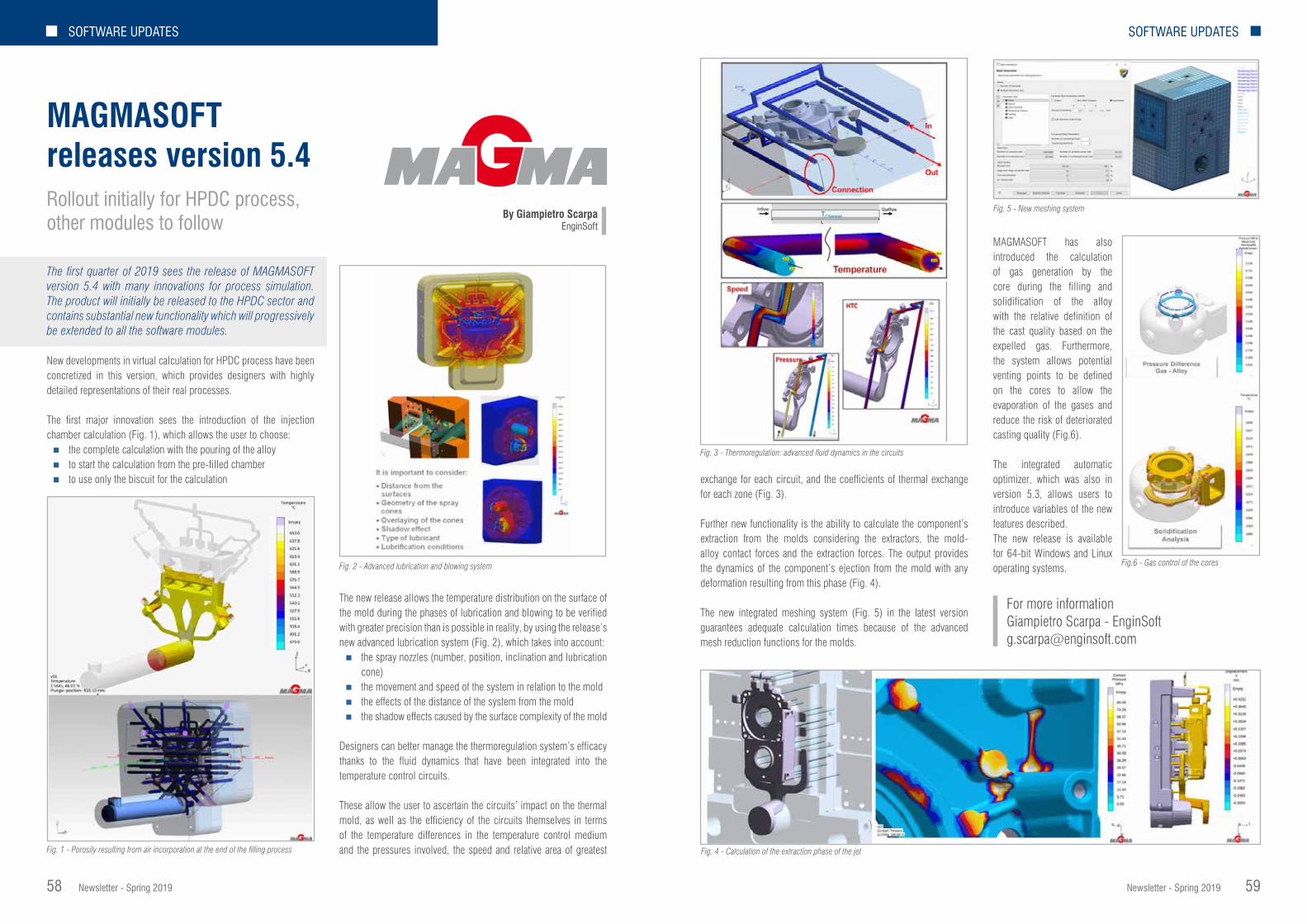
Newsletter - Spring 2019 5958 Newsletter - Spring 2019
The first quarter of 2019 sees the release of MAGMASOFT version 5.4 with many innovations for process simulation. The product will initially be released to the HPDC sector and contains substantial new functionality which will progressively be extended to all the software modules.
New developments in virtual calculation for HPDC process have been concretized in this version, which provides designers with highly detailed representations of their real processes.
The first major innovation sees the introduction of the injection chamber calculation (Fig. 1), which allows the user to choose:n the complete calculation with the pouring of the alloyn to start the calculation from the pre-filled chambern to use only the biscuit for the calculation
The new release allows the temperature distribution on the surface of the mold during the phases of lubrication and blowing to be verified with greater precision than is possible in reality, by using the release’s new advanced lubrication system (Fig. 2), which takes into account: n the spray nozzles (number, position, inclination and lubrication
cone)n the movement and speed of the system in relation to the moldn the effects of the distance of the system from the mold n the shadow effects caused by the surface complexity of the mold
Designers can better manage the thermoregulation system’s efficacy thanks to the fluid dynamics that have been integrated into the temperature control circuits.
These allow the user to ascertain the circuits’ impact on the thermal mold, as well as the efficiency of the circuits themselves in terms of the temperature differences in the temperature control medium and the pressures involved, the speed and relative area of greatest
MAGMASOFT releases version 5.4 Rollout initially for HPDC process, other modules to follow By Giampietro Scarpa
EnginSoft
Fig. 1 - Porosity resulting from air incorporation at the end of the filling process
Fig. 2 - Advanced lubrication and blowing system
exchange for each circuit, and the coefficients of thermal exchange for each zone (Fig. 3).
Further new functionality is the ability to calculate the component’s extraction from the molds considering the extractors, the mold-alloy contact forces and the extraction forces. The output provides the dynamics of the component’s ejection from the mold with any deformation resulting from this phase (Fig. 4).
The new integrated meshing system (Fig. 5) in the latest version guarantees adequate calculation times because of the advanced mesh reduction functions for the molds.
MAGMASOFT has also introduced the calculation of gas generation by the core during the filling and solidification of the alloy with the relative definition of the cast quality based on the expelled gas. Furthermore, the system allows potential venting points to be defined on the cores to allow the evaporation of the gases and reduce the risk of deteriorated casting quality (Fig.6).
The integrated automatic optimizer, which was also in version 5.3, allows users to introduce variables of the new features described. The new release is available for 64-bit Windows and Linux operating systems.
Fig. 5 - New meshing system
Fig.6 - Gas control of the cores
Fig. 3 - Thermoregulation: advanced fluid dynamics in the circuits
Fig. 4 - Calculation of the extraction phase of the jet
SOFTWARE UPDATESSOFTWARE UPDATES
For more informationGiampietro Scarpa - [email protected]

Newsletter - Spring 2019 6160 Newsletter - Spring 2019
Prometech Software, Inc.’s Particleworks ver. 6.2, and Granuleworks ver. 1.1, are now available from EnginSoft.
Particleworks is a liquid flow simulation software based on moving particle simulation (MPS), an innovative meshless calculation method where fluids are shown as a gathering of particles to allow stable and highly-accurate analyses of free surface flows. The software is particularly effective for simulations of oil behavior in powertrains, engine oil cooling, splashing of water around the vehicle, and the mixing of chemicals and resins. Its meshless technology and intuitive interface contribute to more effective product development and design optimization. Particleworks is used worldwide in a broad variety of industries including automotive, electronics, chemical, medical, food, and consumer goods.
Granuleworks is a granule materials simulation software that uses discrete element method (DEM) and is used in a wide assortment of powder processing and powder-based manufacturing processes, such as foods, medicines, chemicals, conveying equipment and electronics, for designing and improving powder equipment due to
its straightforward analyses of powder phenomena such as mixing, conveying, filling and compaction.A number of updated features are shared across the two software packages, including:
Coupling with RecurDyn multi-body dynamics simulation software’s elastic bodiesBoth Particleworks 6.2 and Granuleworks 1.1 enable users to perform simulations with RecurDyn’s bi-directional coupled analysis of elastic and rigid bodies. Large deformation calculations using R-Flex (linear elastic bodies) and F-Flex (non-linear elastic bodies) can be reflected in real-time to both Particleworks’ and Granuleworks’ polygon wall. As RecurDyn calculates the elastic deformation, Particleworks and Granuleworks simultaneously calculate dynamic stress and strain under fluid force.
Evaluation system for analyzing the degree of mixingPowder and granular materials are segregated due to various characteristics, such as their particle size, their surface roughness and their particle shapes. While there have been many studies based on the statistics of mixed state analyses, it was impossible to form correspondences to local mixed states or to the mixed states of micro-components, due to statistical errors. Particleworks and Granuleworks solve this problem by using an evaluation system for the degree of mixing based on entropy. This makes it possible to
Prometech Software releases Particleworks 6.2 and Granuleworks 1.1Native support for NVIDIA Volta’s GPU architecture renewed
By Massimo Galbiati1, Akiko Kondoh2, Werner Nakamachi21. EnginSoft - 2. Prometech Software, Inc.
Fig 1: interaction between fluid and deformable structure
analyze the degree of mixing based on arbitrary spatial resolution, which excludes statistical errors, and is the reason for the two software packages’ potentially wide application beyond that of mixing equipment.
Support for NVIDIA CUDA 9.1Each version update of both Particleworks and Granuleworks sees the solvers renewed and optimized for the latest CPU and GPU
architectures. Thus, Particleworks 6.2 and Granuleworks 1.1 both support NVIDIA Volta’s CUDA 9.1 GPU platform. Volta, developed as a computing engine for computational and data science, is the most powerful GPU architecture available today. The native support for Volta significantly boosts the analysis performance of Particleworks and Granuleworks allowing users to perform large-scale simulations of up to tens of millions of particles.
New SDEM feature in GranuleworksScalable DEM (SDEM) is a new coarse-graining technology for use with the discrete element method that has been developed by Prometech. It is commonly known that stress networks are created within granular materials. SDEM is a theoretical construction that uses the characteristics of these stress networks and can be applied to gravital control systems (the system where contact between the particles is most dominant), facilitating difficult, highly coarse DEM-based simulations.
For more informationMassimo Galbiati - [email protected]
“Prometech Software, Inc. is committed to the continuous development of both Particleworks and Granuleworks and unveiled the newest Particleworks roadmap at the last Prometech CAE Conference in Japan. This will see the development of both new simulation methodologies and new specific applications.”
Massimo Galbiati - EnginSoft
SOFTWARE UPDATESSOFTWARE UPDATES

Newsletter - Spring 2019 6362 Newsletter - Spring 2019
RecurDyn V9R2 introduces some game-changing possibilities in the context of multi flexible body dynamics (MFBD): full flex bodies can now react to thermal loads to account for their thermal deformation; the interface for Particleworks software has been extended to allow for co-simulation between full flex bodies and incompressible fluids; a new solver (called “Advanced Hybrid Integrator”) radically reduces the solution time for several types of models; while many upgrades to the GUI make V9R2 the most usable and powerful version of RecurDyn ever.
Thermal loadsThermal loads can now be applied to a pre-defined set of nodes on full flex bodies. Temperature is defined through expressions, providing unlimited power by enabling the input value to be linked either to time or to other quantities calculated within the model. The RecurDyn solver computes the resulting thermal deformations and considers their influence on the developing dynamics. Thermal stresses and strains can be visualized in the contour plots at the end of the simulation.
Co-simulation of flexible models with ParticleworksRecurDyn was already the only multi-body software enabling the coupled simulation of mechanics and fluid dynamics, however, that capability was restricted to rigid bodies only. Version V9R2 improves the interface between RecurDyn and Particleworks, allowing the use of fully flexible bodies. This establishes a new frontier in multi-body simulation by providing the technology to efficiently reproduce any fluid structure interaction (FSI) in dynamic conditions.
The dedicated post-processor included in the new interface makes it easy to extract many quantities from the simulation: RecurDyn provides access to both the fluid pressure (acting on the walls) and to the stresses/strain generated by the superimposition of
FunctionBay announces the release of RecurDyn V9R2 Introduces game-changing possibilities to multi flexible body dynamics simulations By Fabiano Maggio
EnginSoft
Fig. 1 – Thermal load interface.
Fig. 2 – Von Mises Stress distribution caused by the fluid on the fully flexible body.
Fig. 3 – New interface for particle-based third-party software.
fluid loads and inertial reactions, while Particleworks enables all the fluid properties, including the kinematics of selected particles, to be mapped.
Overall, these added capabilities make it possible to simulate applications that were not possible to tackle before.
The advanced hybrid solverTo date, RecurDyn has included three main solvers: the well-known differential/algebraic system solver (DASSL) provides good stability, even though it introduces excessive numerical damping at high frequencies; the highly-recommended implicit generalized alpha solver’s performance has been balanced by FunctionBay’s developers to maintain stability for low-damped systems while reducing numerical damping in the high-frequency range; the hybrid solver is proprietary technology developed by
FunctionBay which combines implicit and explicit formulations for pre-selected variables to enable the integration of models that include both rigid and flexible bodies. RecurDyn V9R2 provides an Advanced Hybrid Integrator which has been developed to preserve the speed and stability of the proprietary Hybrid solver, while returning the low damping of the implicit generalized alpha solver in the high-frequency range.
The multi co-simulation modeRecurDyn V9R2 also brings new capabilities to its co-simulation mode. Thanks to the functional mock-up interface (FMI), RecurDyn can be connected to multiple and different codes that support this standard. For example, it is possible to combine a hydraulic actuator created in AMESim with a control system developed in MATLAB simulink, to drive a digital prototype built in RecurDyn.
The gear involute contactThe new release of RecurDyn also takes a consistent step toward gear and driveline simulation with the inclusion of the “Gear
Involute Contact”, an analytical type of contact to efficiently solve the tooth-to-tooth interaction of involute gears.This feature uses a pattern of 2D involute profiles to represent the thickness of the teeth, so that the 3D interaction is fully captured.
The new contact type is applicable to spur gears, internal spur gears, helical gears, and internal helical gears.
Acoustics ToolkitV9R2 also includes RecurDyn/Acoustics, a brand new toolkit for acoustics analysis. This module calculates equivalent radiated power (ERP), starting from the outputs of any MFBD simulation. The resulting distribution of the ERP over the surfaces is, in its turn, the starting point for predictive analysis of the noise emitted by mechanical systems.
Julia script for CoLinkRecurDyn V9R2 introduces support for Julia scripting within CoLink’s user-defined blocks. Many users will feel familiar with Julia Script as it is similar to MATLAB language.
General enhancementsV9R2 also includes a number of general enhancements to improve the everyday user experience. The internal mesher has been up-powered to generate better meshes in less time. The new version offers a surface meshing preview, an increased number of re-meshing controls, new mesh healing features and a quality check tool to properly assess the final mesh. Other improvements apply to the belt toolkit, the CAD import interface, the eTemplate, ICF generation, the parameter template, the Activate/Deactivate option for RFlex bodies, the RFI optimizer, and the plot interface. Special features have been also added to pre- and post-process reduced flex and full flex bodies.
For more informationFabiano Maggio - [email protected]
Fig. 4 – Co-simulation scheme including RecurDyn as both master and multiple slaves.
Fig. 5 – Involute profiles checked during solution.
SOFTWARE UPDATESSOFTWARE UPDATES

Newsletter - Spring 2019 6564 Newsletter - Spring 2019
PASS/Nozzle-FEM is a program designed to calculate the stresses and flexibility of nozzle-to-shell junctions using the finite element method (FEM). It also calculates the nozzle’s allowable loads and estimates the strength of the junctions for a wide range of geometric configurations and operating conditions. The program helps engineers to provide higher levels of equipment safety while reducing labor costs at the design stage. It is intended for use by equipment and piping designers and mechanical engineers and can help them to quickly check and satisfy requirements for loads on pressure vessel/equipment nozzles, as well as on non-standard piping fittings. It is recommended for use in design and industrial safety reviews in oil and gas, refineries, petrochemical, chemical, power and other industrial facilities.
Unlike other widely available FEM programs (eg. ANSYS, NASTRAN, COSMOS, etc.), PASS/Nozzle-FEM does not require special training and can be used by any mechanical engineer. It automatically creates the FE mesh and estimates the calculation results. The use of FEM calculations as opposed to semi-analytic methods (i.e. WRC 107/297) expands the application range of the program and increases the accuracy of its analyses.
PASS/Nozzle-FEM performs stress analysis for nozzle junctions of different types (including trunnions) connected to cylindrical and conical shells, as well as for elliptic, hemispherical and flat heads. It takes into account the vessel boundary restraints and loads on the nozzle from the adjacent pipeline. It can calculate nozzle and shell membrane, bending and total stresses. It can also calculate the pipe branch connections to enable a detailed stress analysis of non-standard tees and stub-ins.
In addition to stress and stability analysis, the program also performs nozzle-shell junction flexibility calculations since this flexibility can considerably influence the vessel and piping stresses. During a stress analysis of pipeline systems, nozzle-vessel junctions are often simulated by anchor supports which leads to an overestimation of stresses and tensions. To address this and automatically create
an appropriate non-standard support in the calculation model, the program allows engineers to pass the nozzle-shell junction flexibilities calculated by PASS/Nozzle-FEM into the PASS/START-PROF piping stress analysis program.
The program allows stress estimation using different codes for allowable stresses, including: ASME VIII div.1, 2; EN 13445-3; GOST 34233.1; JB 4732-1995; and PNAE G-7-002-86 (for the equipment and pipelines of nuclear power plants). It supports vessel stress and stability analyses and the reinforcement required of openings under internal pressure. The program also analyzes nozzle-shell junctions operating in corrosive hydrogen sulphide environments.
Major changes to the program kernelIn July 2018, PSRE Co released Nozzle-FEM version 2.15 [1], which introduced several major changes. The company completely reworked the program kernel to improve the program’s speed, extensibility, support for hierarchical models at the logical level, and much more.
The program kernel consists of three main components (Fig. 1), which can be used independently of each other. The object-hierarchical model is intended to be managed by the user, and presents an analysed structure as a tree of objects: for instance, the nozzle is represented as a child object of the supporting shell. In this model, only those geometric data that describe the object itself, and the data required for positioning the child objects are specified.
A geometric model, which is a topological model, so it contains information about curves, surfaces, solids, and the relationships between them, is generated from the object-hierarchy model. This program component uses a licensed C3D geometric kernel [4].
New, extended capabilities of PASS/Nozzle-FEM Improved calculation methods enable better regulatory compliance By Roman Unesikhin, Andrey Krasnokutsky,
Alexey TimoshkinNTP Truboprovod
Fig. 1 - Kernel components of Nozzle-FEM
Currently, a shell-based topological model is used in the Nozzle-FEM kernel, which is built along the middle surface of the shells.
A FE model that consists of the shell’s finite elements is then built based on the geometric model. A system of linear algebraic equations corresponding to the equilibrium conditions of the deformable solid is compiled for FE model.
Previously, the program only ran on 32-bit platforms. To increase the program’s capabilities, the kernel and the FE solver has been redesigned for 64-bit platforms. As a result, from version 2.15, the program only runs on 64-bit versions of MS Windows.
Refined calculation methodsVersion 2.15 also refines the following basic calculation methods: strength, allowable loads on the nozzle, stiffness, and stress intensification coefficients.Two approaches are now used in stiffness (flexibility) calculations: stiffness calculations of the “Supporting shell - nozzle” system (total stiffness), and calculations of stiffness excluding the beam (local stiffness at the place of the nozzle’s tie-in). This second approach is applied for simultaneous work with programs which use a beam FE model (such as PASS/START-PROF [3]) and some equipment modeling (such as vessel shell or tee in PASS/START-PROF [3]). In this case, PASS/Nozzle-FEM builds an equivalent beam model in background, and the local “shell” junction’s stiffness is determined by the difference between the displacements of the shell and the beam models:
where ubi is a calculated value of the i degrees-of-freedom at the end of the nozzle in the beam FE model, and ui is the same in the shell model.
To refine the stress and strain calculation methods, a stress extrapolation procedure was introduced, which solves two problems:n It allows the FE mesh to be condensed in the stress concentration
zones by introducing special zones in which additional refining and alignment of the mesh is performed;
n It increases the convergence of results at different mesh refining levels, reducing design errors (and mitigating the habit of users to not use calculation checks on very fine meshes).
The stress extrapolation procedure is implemented by the Hot Spot Stress method (HSS) [5-8]. HSS uses a linear surface extrapolation (LSE) procedure to calculate the stress at the weld toe (Fig. 2). The selection of the points t1 and t2 by LSE depends on the shell thickness s. This approach stabilizes the process of determining stresses around concentrators and increases the convergence of the results at different mesh refinement levels in the FE model.
For instance, one can compare the results of calculations obtained with the extrapolation procedure and without it using the example of a nozzle tie-in to a cylindrical shell with an axial force of 100 kN applied at the nozzle. In this case, using earlier approaches, one couldn’t determine the maximum total stresses even at the 5th level of mesh refinement (Fig. 3b). The total stresses (membrane + bending) on the outside surface at the first level were 64.1 MPa (Fig. 3a); taking into consideration a mesh coefficient of Km = 1.30, the calculated stresses would be equal to 83.3 MPa. At the same time, the stresses at the fifth level of the mesh were 83.9 MPa (Fig. 3b) and, taking into account a mesh factor of Km = 1.05, the stress would be 88.1 MPa. This demonstrates that the maximum value of total stresses at the first level did not reach the value of the fifth level. The figure below shows that the maximum peak values are not obtained even at the fifth level of the mesh.
Instead, when using the stress extrapolation procedure for this same example (Fig. 4), the first and fifth levels of the mesh produce similar results which exceed the results of the calculations done without applying extrapolation of stresses.
Version 2.16 of PASS/Nozzle-FEM, released in December 2018, offers a new approach to “in Junction” calculations which occasionally causes misunderstanding among users about how stresses are calculated in the welded zone. The “in Junction” option is usually used when the pipe ends at the area of junction into the shell (point “i” in Fig. 5). The pipeline calculation model usually ends on the outside surface of the shell, and calculation loads on the nozzle are obtained at this point.Fig. 2 - Hot spot stress (HSS) method
Fig. 3 - Total (membrane and bending) stresses at the first (a) and fifth (b) levels of the mesh
Fig. 4 - Total (membrane and bending) stresses at the first (a) and fifth (b) mesh levelsusing the stress extrapolation procedure
SOFTWARE UPDATESSOFTWARE UPDATES

Newsletter - Spring 2019 6766 Newsletter - Spring 2019
In versions before 2.16, the most minimal nozzle calculation length possible was taken to build the FE model. After version 2.16, the nozzle length is determined by the condition of sufficient flexibility:
This allows engineers to consider an ovalization of the section at the junction area that corresponds to the “flexible” connection between the pipeline and the shell, and has been obtained from numerous
field tests [9]. In versions up to 2.16, when selecting “in Junction”, the minimal length taken led firstly to a more rigid junction of the pipeline into the shell and secondly to an incorrect determination of the stresses in the junction area since edge effects could occur at the load application point on the nozzle (Fig. 6).
Fig. 7 represents the change curve in the allowable axial force Fy depending on the nozzle length L1, which shows that, in the junction area, at a distance less than 100 mm, edge effects from the load application point appear. Calculation results are given for a tilted nozzle with an inside diameter of 203 mm and 6 mm thickness joining into a cylindrical shell with an inside diameter of 2000 mm and a thickness of 12 mm.
When calculating the strength, the PASS/Nozzle-FEM software automatically converts the loads specified by the user at the junction point into statically equivalent loads, corresponding to a section with a length L1 = Lmin (Fig. 5) [4].
New types of nozzle junctionsThe reworking of the kernel, and the use of the up-to-date C3D geometric kernel for solid modelling has enabled the inclusion of several new types of junctions with beading and weld-in toroidal insertions (Fig. 8). Users can therefore now model stamped and stamp-welded nozzles using PASS/Nozzle-FEM program.
New bearing elementsUnlike with PASS/EQUIPMENT (PASSAT) [2], PASS/Nozzle-FEM did not offer conical transition with displacement of the second end (eccentric transition) for a long time due to difficulties associated with the complexity of its implementation within the program’s old kernel (Fig. 9).Many users also asked for the addition of flat rectangular covers to the program, with which it is possible to model junctions into air-cooled heat exchanger (ACHE) covers, walls of cubic vessels, etc. (Fig. 10).These elements have now been added to the list of calculation models.
Loads and actionsIn order to simulate real loads more correctly, an option has been added to set the hydrostatic pressure required for calculations of
Fig. 5 - “In Junction” calculation model
Fig. 6 - Distribution of total equivalent stresses on the outside surface: a) L=30mm – well-defined edge effect from the load application; a) L=50mm – short length of the nozzle, falls within the area of the edge effect of the load application; c) At the nozzle length obtained by formula (2)
Fig. 7 - A change curve in the allowable axial force Fy depending on the nozzle length L1 for a tilted nozzle in the cylindrical shell.
Fig. 8 - Nozzle with welded-in toroidal insertion.
Fig. 9 - Total (membrane and bending) stresses in a conical shell with displacement of the second end
Fig. 10 - Total (membrane and bending) stresses in a rectangular vessel with nozzle
vertical vessels and tanks, although this load can be set for other types of shells (Fig. 11). Hydrostatic pressure now changes linearly along the vertical axis, where the maximum value is determined at the level of the model’s lowest point. For vertical vessels (tanks), this corresponds to the level of the head.
Thermal strain was another popular and fundamental addition to version 2.16 of the program. This allowed the expansion (deformation) of materials in the structure elements to be considered under the effects of temperature, as well as any additional stresses arising from constrained temperature deformations (different linear expansion coefficients, temperatures, etc.).
Fig. 12a shows the distribution of equivalent stresses in an elliptical head with an internal pressure of 0.5 MPa. The maximum stress value was 86.6 MPa. As an example, the materials on the shell and nozzle were set at different linear thermal expansion coefficients,
with different temperatures on the head (200 °C) and on the nozzle (220 °C). This will generate a temperature deformation constraint and junction stresses will drastically increase (Fig. 12b) in the area of the nozzle, to a maximum stress value of 118.5 MPa.
The ability to consider the effects of temperature has also enabled better compliance with regulatory requirements. For instance, with ASME BPVC.VIII.2, the thermal expansion of materials should be considered when checking the equivalent stresses of the “Secondary Membrane
plus Membrane” category. In GOST 34233.1-2017, while checking with formula (12), it is necessary to consider the additional stresses arising from the effect of temperature:
or while calculating temperatures with formula (13), at which the allowable stresses are defined by the limits of long-term strength or creep:
Updating of codes (regulatory documents)In the development and refinement of the new version of the kernel, a module for strength verification in accordance with various regulatory documents was also reworked, which provides quite flexible and fast processing of updated versions of different codes. As a result, the program is now compliant with ASME BPVC.VIII.1, 2 2017, EN 13445 3:2014 (E) Issue 4 (2017 07), and GOST 342233.1, 6, 10-2017.
RoadmapWith regard to the future, PSRE Co envisions PASS/Nozzle-FEM as an interactive builder of vessels and apparatus on the one hand, and as a possible embedded solution on the other hand. Consequently, a key priority is to rework the PASS/Nozzle-FEM user interface, which will, for example, enable the program to “seamlessly” integrate with the PASS/EQUIPMENT and PASS/START-PROF programs to calculate junctions directly in their environment.
Another possibility is that two software solutions will be available simultaneously: a separate program with advanced options for creating complex models, and an equivalent to the current version with the option of embedding it in the other software. Both will be more functional and interactive than they are now.
References[1] PASS/EQUIP Nozzle — FEM. Strength and flexibility calculation of
nozzle-to-shell junctions using FEM (https://www.passuite.com/equip#nozzle-tab ).
[2] PASS/EQUIP. Strength analysis of vessels, apparatus and heat exchangers (https://www.passuite.com/equip ).
[3] PASS/START-PROF. Quick pipe stress analysis and optimal sizing (https://www.passuite.com/start).
[4] Geometric kernel C3D Modeler (https://c3dlabs.com/en/ ).[5] Fricke, W. Recommended Hot-Spot Analysis Procedure for Structural
Details of Ships and FPSOs Based on Round-Robin FE Analysis [Electron. resource] / W. Fricke // Int’1 J. of Offshore and Polar Engineering. – 2002. – Vol. 12, No. 1. – CD-R.
[6] Maddox, C. J. Hot-Spot Stress Design Curves for Fatigue Assessment of Welded Structures [Electron. resource] / C. J. Maddox // Int’l J. of Offshore and Polar Engineering. – 2002. – Vol. 12, No 2. – CD-R.
[7] Nazari, A. Application of the Hot Spot Stress Method to the Fatigue Assessment of Hollow Section Shiploader Boom Connections [Electron. resource] / A. Nazari, J. Durack // Proc. of 5th Australasian Congr. on Appl. Mechanics ACAM– 2007. – Brisbane, 2007. – CD-R.
[8] Bard, W. T. Fatigue Assessment of Aluminum Ship Details by Hot-Spot Stress Approach [Text] / W. T. Bard, W. Xiaozhi, B. Stig // ABS Technical Papers, 2007. – P. 255-271.
[9] ASME B31J-2017. Stress Intensification Factors (i-Factors), Flexibility Factors (k-Factors), and Their Determination for Metallic Piping Components.
For more informationLivio Furlan - [email protected]
Fig. 11 - Membrane stresses from hydrostatic pressure in a vertical vessel.
Fig. 12 - Total (membrane and bending) stresses in the elliptic head under the influence of: a) internal pressure; b) internal pressure and temperature.
SOFTWARE UPDATESSOFTWARE UPDATES

Newsletter - Spring 2019 6968 Newsletter - Spring 2019
Total Materia, the world’s most comprehensive materials database, continues developing by offering new data sets for key design and material selection decisions to the engineering community. Two new modules, Enviro and Compliance, are now available.
Enviro introduces four complimentary datasets to provide even more breadth and depth to the information provided within the Total Materia platform. Covering corrosion, weatherability, irradiation and different aging effects, Enviro provides a key source of information for the design, manufacture and sale of better-quality products with greater longevity to the market place.In synergy with the primary material databases, Total Metals and PolyPLUS, Enviro facilitates material application decisions by providing a comprehensive understanding of material behaviors under the influence of a range of diverse impacts.
The Compliance module provides a single view of up-to-date global regulations for both materials and substances, allowing businesses to keep pace with the ever-increasing legal obligations related to their products, components and the materials they use. Compliance helps in a variety of complex tasks such as the design and launch of new products, converting existing portfolios to meet regulatory guidelines, approving vendors, controlling materials and more.
Comprising inventory lists, hazard identification, transport information and much more for thousands of materials, Compliance includes international regulations, such as registration, evaluation, authorization and restriction of chemicals (REACH) and restriction of hazardous substances (RoHS), national regulations from the US to Japan, China and Russia, as well as specialized regulations such as those for the food industry, and water and sanitation, all integrated and searchable with material properties information.
Total Materia updated with two new modules Support for aging effects and global regulation compliance By Mariagrazia Vottari
Key to Metals AG
In May 2018, the Juncker Commission announced a third set of measures aimed at transforming the EU into a world leader in the innovation, digitalization, and decarbonization of mobility. This journey began in May 2017 with the “Europe on the Move” vision which was a call to action for all European countries to undertake a socially fair transition towards clean, competitive and connected mobility for all. Among the many initiatives is an integrated policy on the future of road safety and infrastructure safety management. This supranational European approach constitutes a guideline for each country and underlines the importance of facing the challenges of our times with the right tools.
The DISS – Road Safety Centre, based at the University of Parma, was established in September 2010. It is the first research center in Italy that systematically coordinates and unifies the many individual Italian research projects and initiatives on road safety and that provides technical and scientific support to Administrations
and Bodies on all aspects of road safety, including infrastructure, people, vehicles, and roads.
One of the DISS ongoing initiatives to promote road safety is its sponsorship of the “Lorenzo Argenti Degree Award”, named in memory of Lorenzo Argenti, who actively contributed to the foundation of the memorandum of understanding aimed at developing and testing an international management system for the prevention of road accidents, and who died in a road accident at work. This prize, targeted
at graduates of Italian universities, awards thesis contributions to deepening one or more aspects of road safety. The prizes are awarded based on the innovation of the results obtained, adherence to the subject matter of the competition, the validity and rigor of the scientific approach adopted, and the relevance and applicability of the results obtained
This year, the DISS selection board awarded first prize to the thesis “Numerical simulation of smoke propagation and evacuation during a tunnel fire. The Condó Road Tunnel as event scenario” (M. De Rinaldis, S.Gori, A. Malagnino, M. Spagnolo, G. Zavarise), written by Mariarita De Rinaldis who obtained her master’s degree in Civil Engineering at the University of Salento with a mark of 110/110 cum laude, in collaboration with EnginSoft s.p.a, at the FPE Competence Centre’s Emerging Methods and Technologies business unit in Mesagne, Italy. This thesis, which was already recognized by the International CAE Poster Award in October 2018, demonstrates the growing relevance of simulation in infrastructure design and management. The awards were presented by Lorella Montrasio, Director of DISS and Professor of the Department of Engineering and Architecture.
Numerical simulation thesis on road safety wins Lorenzo Argenti Degree AwardAward emphasises role of simulation in infrastructure design and management
PRESS RELEASESOFTWARE UPDATES
For more informationAntonio Parona - [email protected]
For more informationMariarita De Rinaldis - [email protected]
Fire Protection EngineeringWarehouse fire-fighting event
by Sandro Gori EnginSoft
Numerical simulations of fire and smoke propagation are widely used during the early stages of the design process to assess, among other things, the structural behavior of buildings, the fire-resistance properties of the evacuation route and more. For this project, the simulations were developed to represent the initial phase of a fire in a warehouse and included all the intermediate bulk containers (IBC) loaded with liquids that were stored in the building and which were partially involved in the fire.
Find out more on the next issue of EnginSoft Newsletter - Summer 2019

Newsletter - Spring 2019 7170 Newsletter - Spring 2019
PRESS RELEASE
for SOLIDWORKS®. This front-loading CFD software includes the most in-demand functions at design sites and will allow engineers to more easily and effectively perform trial-and-error tests. The last announcement concerned Prometech’s vision for cloud-enhanced technology implementations, on which more information will be forthcoming in the near future.After the plenary session, the conference divided into five different sessions and the targeted GPU Computing Workshop for Advanced Manufacturing session, with their respective lectures and speakers; the MPS User session, the MPS Academic session, the AI-driven CAE session, the Front-Loading session and the AI & Deep Learning session.The MPS User session opened with the introduction of the enthusiastically received development roadmaps for Particleworks and Granuleworks. This was followed by speakers from the CAE industry sharing their latest insights and case studies. Notable highlights of this session were the contributions of the first international guest speakers: Massimo Galbiati of EnginSoft S.p.A. who spoke on the industrial applications of moving particle simulation in the automotive and the transportation sectors, and Chulmin Ahn of Hyundai Motor Company who spoke about the development of the churning oil path optimization process. Not only did they contribute to the CAE industry by sharing their insights, but they also contributed to the further internationalization of the conference. There were also plenty of lectures featuring DEM powder simulations and user cases for which there has been a noticeable increase in domestic demand, such as composite design powered by cloud computing technology and landslide simulations.The MPS Academic Session focused on the latest research and non-business applications of Moving Particle Method thrombosis biomechanics, arc welding simulations, refined schemes and calculations methods, multi-physics CFD simulation by the MPS method including icing, deposition and suppression of tsunamis, a state-of-the-art DEM-CFD simulation of gas-solid two-phase flows, and multi-resolution techniques for reducing computation time in particle methods and their applications, as well as a lot of other important research that will be very valuable in the future.This year’s conference also introduced an AI-driven CAE Session. Although AI is already broadly present in many industries, its application to CAE is still rather new. The introduction of AI to CAE via deep learning and cloud computing is a very promising method to improve product design efficiency and to reduce calculation times using predictions. Needless to say, the AI-driven CAE session attracted the most attention and the highest number of participants during the conference. Speakers from both the private and the academic sectors shared their insights on case studies using AI-driven CAE, the future of CAE, and how cloud computing and deep learning may contribute to tackling challenges and achieving that goal.
The addition of the 3D CAD-tool integrated Particleworks for SOLIDWORKS to Prometech’s product line in January 2019, forecasts a trend that will see Particleworks, already essentially adopted by the automotive industry, being more commonly used during the early design stage. In support of this trend, the Front-Loading session
focused on how MPS can be utilized at the initial design stage to save time and costs.During his presentation, Mitsuhiro Mori of Kozo Keikaku Engineering Inc., spoke on development efficiency while Simon Harbeke, EnginSoft GmbH, spoke on a robust CAD-integrated approach for simulating free surface flows using the MPS method.
The GPU2018 GPU Computing Workshop was a simultaneously organized event that focused on machine learning methods for AI development with an emphasis on deep learning, GPGPU experiments and quantum computing. Kuninobu Sasaki, Japan Country Manager and vice president for Worldwide Field Operations of NVIDIA, who led a session on the evolutions of GPU computing starting from CUDA to how GPU computing is accelerating AI and HPCs today, was a notable speaker at the GPU workshop.A post-conference reception was held in the exhibition area which also housed the product displays of two dozen companies. This event kicked off after professor Seiichi Koshizuka’s keynote speech and Professor Genki Yagawa of the University of Tokyo’s closing address. The reception was the perfect place to see old and new faces, to exchange insights and knowledge and to get into deeper discussions with the numerous speakers of the event.Current and potential users were happy to hear about the potentials in the development roadmaps of Particleworks and Granuleworks. Many participants also appreciated the rich information from the broad variety of companies gathered in one day and its contribution to assisting them to tackle their own simulation challenges.
With over one thousand participants, the latest edition of the Prometech Simulation Conference and GPU Computing Workshop have been the most successful to date. We are intrigued as to what the 2019 edition, that will be held on Friday December 6th in Tokyo, will contribute to the simulation industry.
For more information about PSC 2018: https://www.prometech-sc.com/2018_en.html
For more informationMassimo [email protected]
The Prometech Simulation Conference is an annual Conference held at the Tokyo International Forum and co-organized by Prometech Software, Inc., developers of the advanced fluid simulation software Particleworks, the advanced simulator for granular materials Granuleworks, and GDEP Solutions, Inc. The Conference is a growing hub of information that gathers the latest in-depth news on the simulation industry with a focus on meshless CFD simulation, research and user cases from a broad variety of companies and academic institutions, in addition to the latest developments in artificial intelligence (AI) and deep learning using GPU computing in Tokyo, Japan.At the 2018 event (PSC2018), representatives of both the Japanese public and private sectors, including company leaders, academic researchers and scholars, delivered talks on research and developments in the CAE industry and users of Prometech’s Particleworks and Granuleworks presented their case studies. This year’s theme was a progressive mix of simulation, and visualization technology, AI and simulation accelerating GPU computing. This is the 7th edition of the Prometech Simulation Conference, which, thanks to its annually-increasing number of participants and over 40 sessions and lectures, has become one of the leading CAE industry events in Japan.Some of this year’s speakers included: Professor Noriko Arai of the Information and Society Research Division of the National Institute of Informatics who spoke on “AI: its possibilities and limitations – preparing society and manufacturing for AI”, Masayuki Ishizaki, CEO of Ascent Robotics, Inc. who presented “We make machines that think”, Professor Seiichi Koshizuka of the University of Tokyo,
who spoke on the distinct particle methods studies of 2018 and also went into detail on fluid-rigid body coupling, the arbitrary Lagrangian-Eulerian method, high accuracy techniques and future prospects on the particle methods, and Ryutaro Okada, Chief Administrative Officer of the Japan Deep Learning Association who focused on the
future of Deep Learning’s industrial applications.During the opening session, Toshimitsu Fujisawa, Prometech Software, Inc.’s CEO, shared his insights on the company’s future business direction and strategic partnerships and made three announcements concerning the company’s business. The first announcement concerned a new collaboration between Prometech and ANSYS, which will bring more wide-ranging Multiphysics solutions to the market; in the second, he disclosed that Prometech will be adding Particleworks for SOLIDWORKS to its product line, a new entry version of Particleworks developed as an add-in tool
Report back from 2018 Prometech Simulation Conference and GPU Computing Workshop in JapanOver 1,000 attendees at 7th edition of this leading CAE event in Japan
PRESS RELEASE

THE ENGINEERING SIMULATION PATHTO DIGITAL TRANSFORMATION
Vicenza, ITALYVicenza Convention Centre @Fiera di Vicenza
2019, 28 - 29 OCTOBER
www.caeconference.com
35th INTERNATIONALCAE CONFERENCE AND EXHIBITION
Exchange ideas and technical know-howNetwork with peers and thought leadersGain new knowledge and know-howExplore new technologies, research and methodologiesIdentify talented new engineers