News-driven inflation expectations and

information rigidities∗

Vegard H. Larsen† Leif Anders Thorsrud‡

Julia Zhulanova§

This version: February 12, 2020

Preliminary. Please do not distribute

Abstract

Using a large news corpus and machine learning algorithms we inves-

tigate the role played by the media in the expectations formation process

of households, and conclude that the news topics media report on are

good predictors of both inflation and inflation expectations. In turn,

in a noisy information model, augmented with a simple media channel,

we document that the time series features of relevant topics help ex-

plain the time-varying information rigidity among households. As such,

we provide a novel estimate of state dependent information rigidities,

∗This article should not be reported as representing the views of Norges Bank. The viewsexpressed are those of the authors and do not necessarily reflect those of Norges Bank. Com-ments by the editor, one anonymous referee, and Kristoffer Nimark improved the quality ofthis paper considerably. We also thank Hilde C. Bjørnland, Paul Beaudry, Drago Bergholt,Gunnar Bardsen, Olivier Coibion, Oscar Jorda, Michael McMahon, Francesco Ravazzolo,and Mathias Trabandt for valuable comments. Comments from conference participants atNorges Bank, the Frisch Center, DIW Berlin, Danmarks Nationalbank also helped improvethe paper. This work is part of the research activities at the Centre for Applied Macroe-conomics and Commodity Prices (CAMP) at the BI Norwegian Business School. We aregrateful to the Dow Jones Newswires Archive for sharing their data with us for this researchproject. Declarations of interest: none.†Norges Bank and Centre for Applied Macroeconomics and Commodity Prices, BI Nor-

wegian Business School. Email: Vegard-Hoghaug.Larsen@norges-bank.no‡Corresponding author. Centre for Applied Macroeconomics and Commodity Prices, BI

Norwegian Business School. Email: leif.a.thorsrud@bi.no§Centre for Applied Macroeconomics and Commodity Prices, BI Norwegian Business

School. Email: julia.zhulanova@bi.no

1

and present new evidence highlighting media’s role for understanding

inflation expectations and information rigidities.

JEL-codes: C11, C53, D83, D84, E13, E31, E37

Keywords: Expectations, Media, Machine Learning, Inflation

2

1 Introduction

The fourth estate, i.e., the news media, plays an important role in society

and is a primary source of information for most people.1 In macroeconomics,

expectations are center stage. But, expectations are shaped by information,

and information does not travel unaffected through the ether. Rather, it is

digested, filtered, and colored by the media. Surprisingly, however, the poten-

tial independent role of the media in the expectation formation process has

received relatively little attention in macroeconomics.

This paper builds on a growing literature providing evidence in favor of in-

formation rigidities rather than full-information rational expectations (FIRE;

Coibion and Gorodnichenko (2012), Dovern et al. (2015), Coibion and Gorod-

nichenko (2015), Armantier et al. (2016)), and investigates the relationship

between news and households’ inflation expectations in such settings.

In particular, we take the view that agents make endogenous information

choices (Sims (2003), Woodford (2009), Mackowiak and Wiederholt (2009)),

but that no agent has the resources to monitor all the events potentially rele-

vant for her decision, and thus delegate their information choice to specialized

news providers, who report only a curated selection of events. As formalized in

Nimark and Pitschner (2019), the media act as “information intermediaries”

between agents and the state of the world.2 Two implications of these views

are that: i) media coverage should predict households’ inflation expectations,

and ii) the degree of information rigidity, as defined more precisely below, will

be time-varying and a function of media coverage.

These implications are tested in two stages. First, the predictive relation-

ship between news and expectations is addressed. To this end, we hypothesize

that when the media writes extensively about topics related to, e.g., technol-

ogy or health, even without explicitly mentioning terms related to inflation,

this reflects that something is happening in these areas that could potentially

have economy-wide effects and might therefore also affect inflation expecta-

1See, for example, Blinder and Krueger (2004), Curtin (2007), and Fullone et al. (2007).2Rather than agents deciding ex-ante on the expected usefulness of a particular signal, as in,e.g., the costly information literature (Grossman and Stiglitz (1980)), knowledge of eventsis jointly determined ex-post through a delegated information choice mechanism.

3

tions. In turn, this conjecture is made operational using a Latent Dirichlet

Allocation (Blei et al. (2003)) model and a large news corpus from the Dow

Jones Newswires Archive (DJ) to construct 80 time series measures of the news

topics the media write about, i.e., the different types of news reporting.

Using penalized linear regressions to handle the high-dimensional predic-

tive problem, and focusing on inflation and households’ inflation expectations,

measured by the University of Michigan Surveys of Consumers (MSC), we find

that many of the news topics written about in the media have high predictive

power for both inflation and expectations. There is also a large intersection in

the selected topic sets for these two outcome variables, and our results imply

that relevant news coverage helps households form more accurate expectations.

Furthermore, the narrative realism of the approach is good. Topics about,

e.g., (IT) technology and health, significantly affect households’ inflation ex-

pectations. Additional results strongly indicate that this type of textual data

contains information not captured by a large set of roughly 130 conventional

economic indicators, suggesting that the media is an important information

source for households. In contrast, but following the intuition that the media

matters foremost for households and less so for professionals, there is little ev-

idence for a relationship between news topics and inflation expectations from

the Survey of Professional Forecasters (SPF).

The MSC micro-data is used to further validate the news-topic-based ap-

proach, and shows that the predictive relationship between news topics and

expectations align well with conventional stereotypes and what we know about

expenditure patterns and media consumption habits. News related to health

and politics, for example, tends to be more important for elderly survey re-

spondents than for young people.

Turning to information rigidities, we augment the noisy information frame-

work in Coibion and Gorodnichenko (2015) by allowing for state dependence

in the degree of information rigidity, and an explicit, but simple, role for the

media. The mechanics of the model are straight forward. When an important

event happens, media coverage potentially becomes more persistent, and the

signal less noisy, and thereby easier to filter for the agents. Accordingly, in-

formation rigidity is reduced as agents put more weight on new information

4

relative to their previous forecasts.

Testing these predictions empirically supports the media channel view.

There is high-frequency time variation in information rigidity, and this varia-

tion can be explained by the time series properties of relevant news coverage,

as the theory predicts. We further show, in a falsification experiment, that

this result is unlikely to be obtained by chance, and using properties of infla-

tion itself, or other economic indicators with predictive power for households’

expectations, does not deliver theory-consistent results.

The contribution of our analysis is threefold. First, by analyzing me-

dia’s role in the expectation formation process, our analysis speaks directly

to work by Doms and Morin (2004), Pfajfar and Santoro (2013), Lamla and

Lein (2014), Drager and Lamla (2017), and Ehrmann et al. (2017). The epi-

demiological model of inflation expectations by Carroll (2003) is particularly

well known. However, we make an important contribution in how we use text

as data in this setting. In contrast to the earlier literature, where analyses

have been based on counting inflation terms in the news to measure media

(inflation) intensity or survey variables measuring whether people have heard

news about prices, we take a topic-based approach. And, indeed, this approach

delivers results in accordance with our media mechanism, while the traditional

text- and survey-based methods do not.

Second, we are the first to investigate the relationship between information

rigidities and news within a well-established theory-based testing framework

(Coibion and Gorodnichenko (2015)). This allows us to directly test the null

of FIRE versus the alternative news-driven information rigidity view.

Third, we provide direct evidence of high-frequency time-variation in the

degree of information rigidity among households in the U.S.. As such, our

results complement Loungani et al. (2013), Coibion and Gorodnichenko (2015),

and Dovern et al. (2015), who document low-frequency changes in information

rigidity among professionals and in international panels.

In sum, the analysis conducted here provides positive evidence in favor

of the state-dependent information rigidity view, but emphasizes the role of

information providers. For this reason, the analysis also speaks to the literature

trying to identify the causal effect of the media. This has been relatively

5

unexplored in macroeconomics, but has received much more attention in other

branches of the literature and in other sciences (Gentzkow et al. (2011), Shiller

(2017), King et al. (2017), Prat (2018)).

2 Expectations and news

To study the relationship between expectations and news, Section 2.1 describes

the news corpus and how the textual data is transformed into quantitative time

series. The predictive results are presented in Section 2.2.

2.1 The news

Our news media corpus consists of roughly five million news articles, written

in English, from the Dow Jones Newswires Archive (DJ), covering the period

1990 to 2016. The database covers a large range of Dow Jones’ news services,

including content from The Wall Street Journal.

Arguable, the DJ includes only a subset of news households consume. Still,

news stories relevant for inflation are undoubtedly well covered by this type

of business news. The Dow Jones company, and its flagship publication, The

Wall Street Journal, is also one of the largest newspapers in the U.S. in terms

of circulation. This means that it has a large footprint in the U.S. media

landscape, and it is likely that its news coverage spills over to news sources

that households follow more directly, e.g., television, or smaller news outlets

(King et al. (2017)). While minor news events might not be covered by this

data source, major economic or political events are surely covered by both DJ

and other media outlets households might follow.

To make our news-topic-based hypothesis operational, we use a Latent

Dirichlet Allocation (LDA) model (Blei et al. (2003)), where each article is

treated as a mixture of topics and each topic is treated as a mixture of words.

The LDA is one of the most popular topic models in the Natural Language

Processing (NPL) literature because of its simplicity, and because it has proven

to classify text in much the same manner as humans would (Chang et al.

(2009)). Thus, the LDA transforms something large and complex, i.e., the

6

US T75: Aviation US T2: Education US T77: Transactions

US T39: Health US T45: Internet US T47: The White House

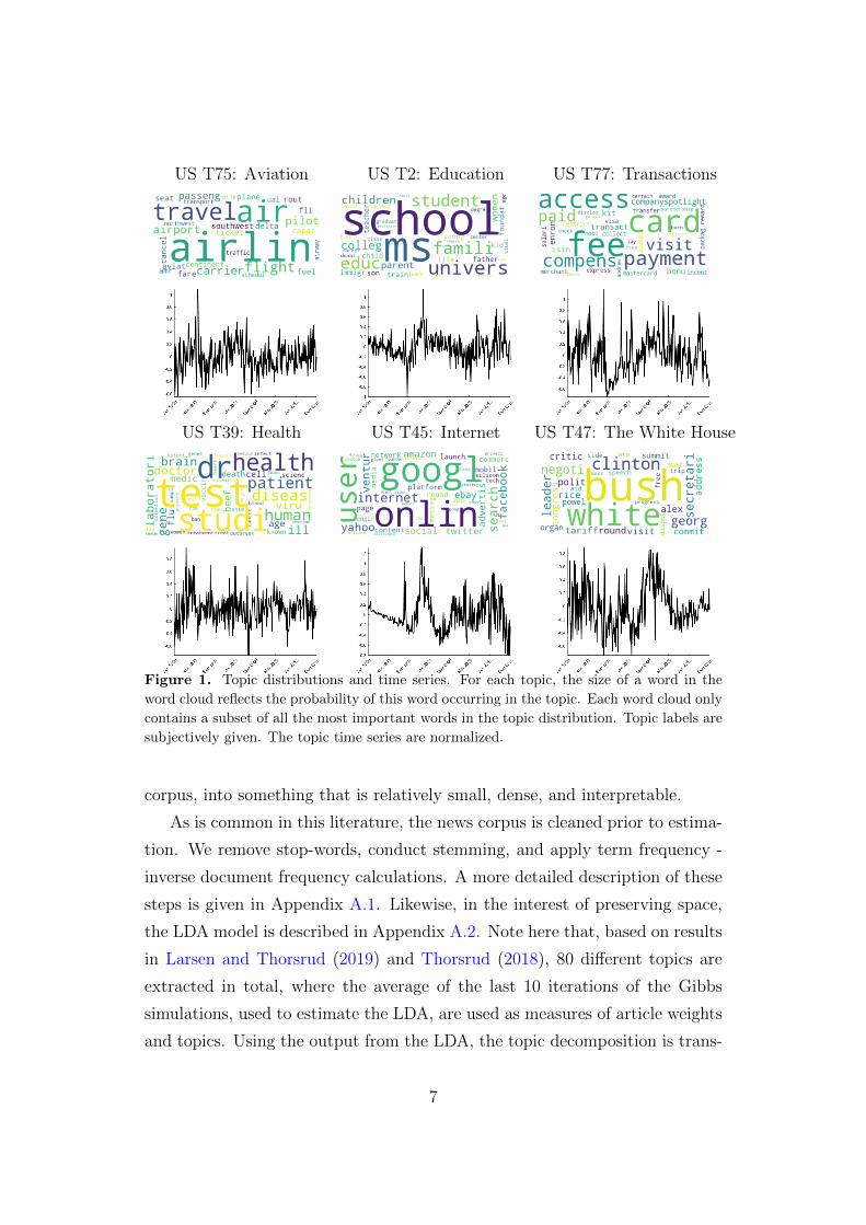
Figure 1. Topic distributions and time series. For each topic, the size of a word in the

word cloud reflects the probability of this word occurring in the topic. Each word cloud only

contains a subset of all the most important words in the topic distribution. Topic labels are

subjectively given. The topic time series are normalized.

corpus, into something that is relatively small, dense, and interpretable.

As is common in this literature, the news corpus is cleaned prior to estima-

tion. We remove stop-words, conduct stemming, and apply term frequency -

inverse document frequency calculations. A more detailed description of these

steps is given in Appendix A.1. Likewise, in the interest of preserving space,

the LDA model is described in Appendix A.2. Note here that, based on results

in Larsen and Thorsrud (2019) and Thorsrud (2018), 80 different topics are

extracted in total, where the average of the last 10 iterations of the Gibbs

simulations, used to estimate the LDA, are used as measures of article weights

and topics. Using the output from the LDA, the topic decomposition is trans-

7

formed into time series, measuring how much each topic is written about at

any given point in time. Finally, the tone of the news is computed, using a

simple dictionary-based approach and output from the topic model, to sign-

adjust the topic frequencies. A more detailed description of this latter step is

relegated to Appendix A.3.

To build intuition, Figure 1 illustrates the output from the above steps

for six of the 80 topics. A full list of the estimated topics is given in Table

B.1, in Appendix B. First, the LDA produces two outputs; one distribution of

topics for each article in the corpus, and one distribution of words for each of

the topics. The latter distributions are illustrated using word clouds in Figure

1. A bigger font illustrates a higher probability for the terms. As the LDA

estimation procedure does not give the topics any name, labels are subjectively

given to each topic based on the most important terms associated with each

topic. How much each topic is written about at any given point in time, and

its tone, is illustrated in the graphs below each word cloud. The graphs should

be read as follows: Progressively more positive (negative) values means the

media writes more about this topic, and that the tone of reporting on this

topic is positive (negative).

2.2 News-driven inflation expectations?

The existing literature is largely silent about which types of news households

(on average) pay attention to in relation to inflation.3 Accordingly, we map the

high-dimensional news topic dataset to inflation expectations using the Least

Absolute Shrinkage and Selection Operator (LASSO; Tibshirani (1996)). The

LASSO method shrinks parameter estimates for unimportant variables towards

zero, thereby encouraging simple and sparse models.

More formally, we run penalized linear predictive regressions like:

Ftπt+12,t+1 = a+M∑n=1

bnNTn,t−1 + εt, (1)

3If anything, news coverage about a primary candidate, monetary policy, is potentially inef-fective because households in general are found to be poorly informed about central bankpolicies (see Coibion et al. (2019) and the references therein).

8

where Ftπt+12,t+1 is households’ expectations, at time t, of inflation over the

next year, and M is the number of news topics NTn,t−1. All variables are

lagged one period relative to Ftπt+12,t+1 to avoid simultaneity issues and look-

ahead biases. The amount of regularization is optimized by setting the LASSO

shrinkage parameter using 5-fold cross-validation, and all variables are stan-

dardized prior to estimation. In line with the predictive purpose of the LASSO,

we focus on partial R2 statistics and significance levels, computed using a post-

LASSO routine on the selected variable set (Belloni and Chernozhukov (2013)),

when reporting the results. Finally, as a benchmark control variable, lagged

CPI inflation is always included in the regressions (irrespective of whether or

not it is selected by the LASSO).

9

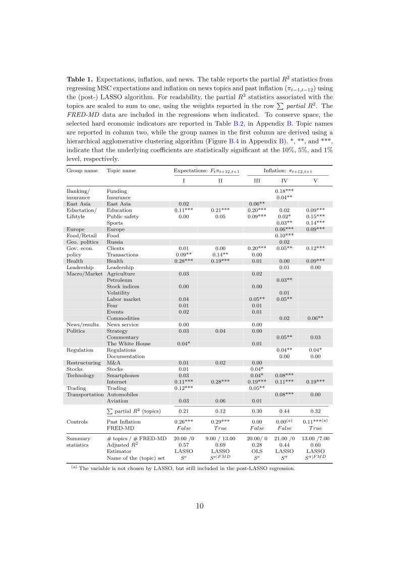
Table 1. Expectations, inflation, and news. The table reports the partial R2 statistics from

regressing MSC expectations and inflation on news topics and past inflation (πt−1,t−12) using

the (post-) LASSO algorithm. For readability, the partial R2 statistics associated with the

topics are scaled to sum to one, using the weights reported in the row∑

partial R2. The

FRED-MD data are included in the regressions when indicated. To conserve space, the

selected hard economic indicators are reported in Table B.2, in Appendix B. Topic names

are reported in column two, while the group names in the first column are derived using a

hierarchical agglomerative clustering algorithm (Figure B.4 in Appendix B). *, **, and ***,

indicate that the underlying coefficients are statistically significant at the 10%, 5%, and 1%

level, respectively.

Group name Topic name Expectations: Ftπt+12,t+1 Inflation: πt+12,t+1

I II III IV V

Banking/ Funding 0.18***insurance Insurance 0.04**East Asia East Asia 0.02 0.06**Eductation/ Education 0.11*** 0.21*** 0.20*** 0.02 0.09***Lifstyle Public safety 0.00 0.05 0.09*** 0.02* 0.15***

Sports 0.03** 0.14***Europe Europe 0.06*** 0.09***Food/Retail Food 0.10***Geo. politics Russia 0.02Gov. econ. Clients 0.01 0.00 0.20*** 0.05** 0.12***policy Transactions 0.09** 0.14** 0.00Health Health 0.28*** 0.19*** 0.01 0.00 0.09***Leadership Leadership 0.01 0.00Macro/Market Agriculture 0.03 0.02

Petroleum 0.03**Stock indices 0.00 0.00Volatility 0.01Labor market 0.04 0.05** 0.05**Fear 0.01 0.01Events 0.02 0.01Commodities 0.02 0.06**

News/results News service 0.00 0.00Politics Strategy 0.03 0.04 0.00

Commentary 0.05** 0.03The White House 0.04* 0.01

Regulation Regulations 0.04** 0.04*Documentation 0.00 0.00

Restructuring M&A 0.01 0.02 0.00Stocks Stocks 0.01 0.04*Technology Smartphones 0.03 0.04* 0.08***

Internet 0.11*** 0.28*** 0.19*** 0.11*** 0.19***Trading Trading 0.12*** 0.05**Transportation Automobiles 0.08*** 0.00

Aviation 0.03 0.06 0.01∑partial R2 (topics) 0.21 0.12 0.30 0.44 0.32

Controls Past Inflation 0.26*** 0.29*** 0.00 0.00(a) 0.11***(a)

FRED-MD False True False False True

Summary # topics / # FRED-MD 20.00 /0 9.00 / 13.00 20.00/ 0 21.00 /0 13.00 /7.00statistics Adjusted R2 0.57 0.69 0.28 0.44 0.60

Estimator LASSO LASSO OLS LASSO LASSO

Name of the (topic) set Se Se|FMD Se Sπ Sπ|FMD

(a) The variable is not chosen by LASSO, but still included in the post-LASSO regression.

10

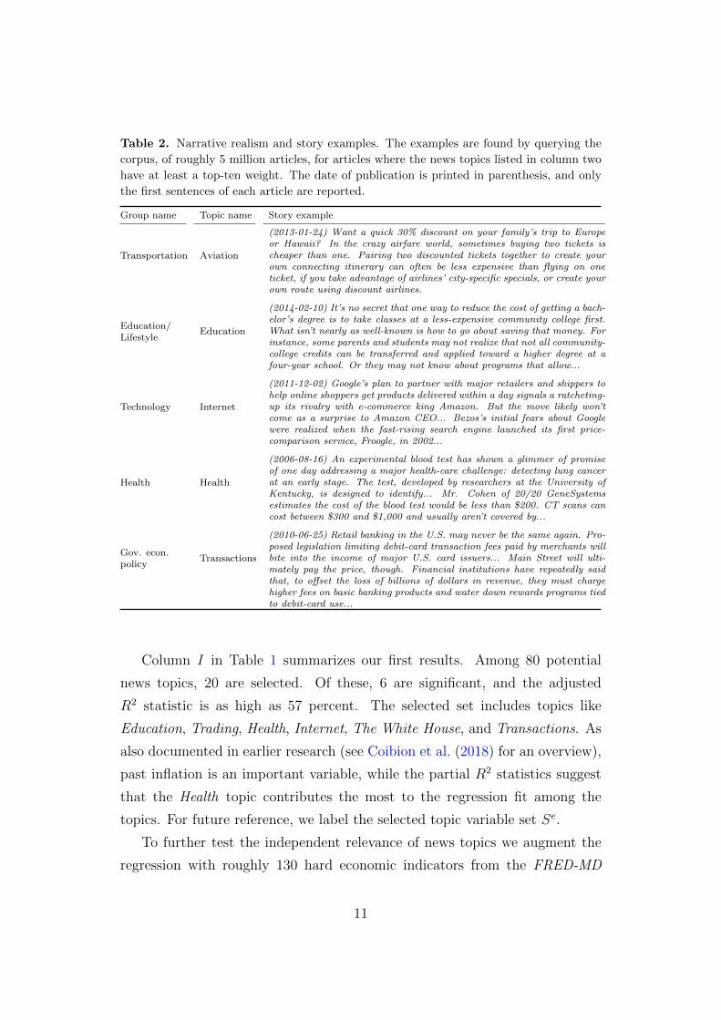
Table 2. Narrative realism and story examples. The examples are found by querying the

corpus, of roughly 5 million articles, for articles where the news topics listed in column two

have at least a top-ten weight. The date of publication is printed in parenthesis, and only

the first sentences of each article are reported.

Group name Topic name Story example

Transportation Aviation

(2013-01-24) Want a quick 30% discount on your family’s trip to Europeor Hawaii? In the crazy airfare world, sometimes buying two tickets ischeaper than one. Pairing two discounted tickets together to create yourown connecting itinerary can often be less expensive than flying on oneticket, if you take advantage of airlines’ city-specific specials, or create yourown route using discount airlines.

Education/Lifestyle

Education

(2014-02-10) It’s no secret that one way to reduce the cost of getting a bach-elor’s degree is to take classes at a less-expensive community college first.What isn’t nearly as well-known is how to go about saving that money. Forinstance, some parents and students may not realize that not all community-college credits can be transferred and applied toward a higher degree at afour-year school. Or they may not know about programs that allow...

Technology Internet

(2011-12-02) Google’s plan to partner with major retailers and shippers tohelp online shoppers get products delivered within a day signals a ratcheting-up its rivalry with e-commerce king Amazon. But the move likely won’tcome as a surprise to Amazon CEO... Bezos’s initial fears about Googlewere realized when the fast-rising search engine launched its first price-comparison service, Froogle, in 2002...

Health Health

(2006-08-16) An experimental blood test has shown a glimmer of promiseof one day addressing a major health-care challenge: detecting lung cancerat an early stage. The test, developed by researchers at the University ofKentucky, is designed to identify... Mr. Cohen of 20/20 GeneSystemsestimates the cost of the blood test would be less than $200. CT scans cancost between $300 and $1,000 and usually aren’t covered by...

Gov. econ.policy

Transactions

(2010-06-25) Retail banking in the U.S. may never be the same again. Pro-posed legislation limiting debit-card transaction fees paid by merchants willbite into the income of major U.S. card issuers... Main Street will ulti-mately pay the price, though. Financial institutions have repeatedly saidthat, to offset the loss of billions of dollars in revenue, they must chargehigher fees on basic banking products and water down rewards programs tiedto debit-card use...

Column I in Table 1 summarizes our first results. Among 80 potential

news topics, 20 are selected. Of these, 6 are significant, and the adjusted

R2 statistic is as high as 57 percent. The selected set includes topics like

Education, Trading, Health, Internet, The White House, and Transactions. As

also documented in earlier research (see Coibion et al. (2018) for an overview),

past inflation is an important variable, while the partial R2 statistics suggest

that the Health topic contributes the most to the regression fit among the

topics. For future reference, we label the selected topic variable set Se.

To further test the independent relevance of news topics we augment the

regression with roughly 130 hard economic indicators from the FRED-MD

11

database and re-estimate the LASSO. The FRED-MD is compiled by Mc-

Cracken and Ng (2016) and is a much used dataset containing (leading) in-

dicators covering the stock market, interest rates and exchange rates, prices,

income, consumption, and the labor market (Appendix C). As seen from col-

umn II in Table 1, the adjusted R2 statistic increases for this larger model, but

not by a very large margin. Fewer topics are also selected, but the significant

topics in the news-only regression tend to stay significant.4

The topics might not have been given names by us that intuitively link

them to inflation expectations. Still, Table 2 shows that the narrative realism

of the approach is good. The table contains examples selected by querying the

news corpus, of roughly five million articles, for articles where topics important

for expectations have a particularly high weight. The Education story, for

example, talks about expenses, while the Health and Transactions stories talk

about costs and fees. Media coverage related to these types of news might

all plausibly affect how households consider inflation developments. As an

alternative, to help interpretation, one could interpret each topic as belonging

to clusters of higher order abstractions, like, politics, technology, etc.. The

first columns in Table 1 and 2 illustrate this, where a clustering algorithm has

been used to group the topics into broader categories (Figure B.4 in Appendix

B). For example, the Internet topic is automatically grouped together with the

Smartphones and Software topics, making it apparent that these news types

are (IT) technology related.

In line with our motivation for the topic-based approach, none of the stories

listed in Table 2 actually contain explicit inflation terms. In contrast, the

conventional method used to measure the intensity of media reporting relevant

for inflation expectations has been to count the number of terms related to

inflation in the corpus’ articles. To more formally compare approaches, we

construct a traditional media measure by counting terms related to inflation

in articles using the wild-card search inflation* (Figure B.1 in Appendix B)

and include this variable in the LASSO together with the other variables.

4As illustrated in Table B.2, in Appendix B, among the hard economic indicators selected aremany variables already focused on in the earlier literature, such as, production indicators(Ehrmann et al. (2017)), volatility measures (Drager and Lamla (2017)), and consumersentiment (Doms and Morin (2004)).

12

Doing so, we observe it is not selected.

2.3 Expectations and inflation

Economic theory, like the New Keynesian Phillips Curve, suggest there should

be a strong relationship between inflation expectations and actual inflation,

even in the presence of information rigidities (Coibion et al. (2018)). This is

also the case here. When regressing CPI inflation on the lagged news topics

selected in the LASSO regression reported in column I in Table 1, half of the

significant topics remain significant (column III ). Allowing all the news topics

to enter the variable selection problem results in a similarly sized set of topics,

while the adjusted R2 statistic increases from 0.28 to 0.44 (column IV ). Thus,

using the news topics relevant for households only reduces the model fit by

roughly 35 percent. These results are robust to controlling for all the hard

economic indicators in the variable selection problem. As above, topics in the

Macro/Market group typically drop out when controlling for the FRED-MD

data, but almost 60 percent of the news topics in the selected set Se|FMD

for households’ expectations (column II ) are in the selected set Sπ|FMD for

inflation (column V ).

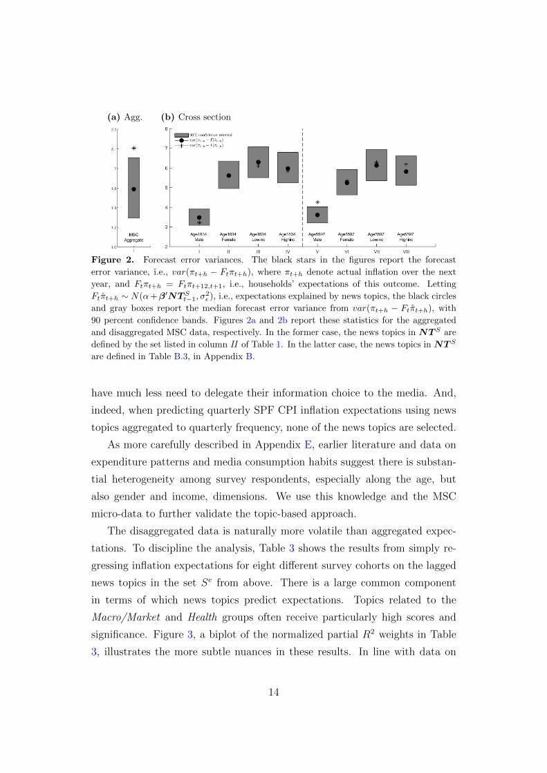
From a forecasting perspective, Figure 2a shows that households’ have a

forecast error variance above 2. Using the part of expectations explained by the

news topics when computing this statistic improves forecasting performance by

roughly 10 percent, i.e., media coverage helps households form more accurate

expectations. Additional results presented in Appendix D document that the

significant predictive relationship between inflation, expectations, and news

topics withstands out-of-sample evaluation.

2.4 The Survey of Professional Forecasters and cross

sectional differences

It is interesting to contrast our results with those obtained if households’ ex-

pectations in (1) are replaced by expectations from SPF. A priori we conjecture

that professional forecasters surely know and follow actual CPI inflation and

13

(a) Agg. (b) Cross section

Figure 2. Forecast error variances. The black stars in the figures report the forecast

error variance, i.e., var(πt+h − Ftπt+h), where πt+h denote actual inflation over the next

year, and Ftπt+h = Ftπt+12,t+1, i.e., households’ expectations of this outcome. Letting

Ftπt+h ∼ N(α+β′NT St−1, σ2ε ), i.e., expectations explained by news topics, the black circles

and gray boxes report the median forecast error variance from var(πt+h − Ftπt+h), with

90 percent confidence bands. Figures 2a and 2b report these statistics for the aggregated

and disaggregated MSC data, respectively. In the former case, the news topics in NT S are

defined by the set listed in column II of Table 1. In the latter case, the news topics in NT S

are defined in Table B.3, in Appendix B.

have much less need to delegate their information choice to the media. And,

indeed, when predicting quarterly SPF CPI inflation expectations using news

topics aggregated to quarterly frequency, none of the news topics are selected.

As more carefully described in Appendix E, earlier literature and data on

expenditure patterns and media consumption habits suggest there is substan-

tial heterogeneity among survey respondents, especially along the age, but

also gender and income, dimensions. We use this knowledge and the MSC

micro-data to further validate the topic-based approach.

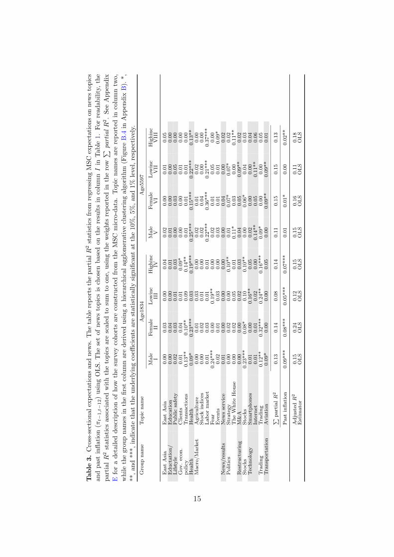
The disaggregated data is naturally more volatile than aggregated expec-

tations. To discipline the analysis, Table 3 shows the results from simply re-

gressing inflation expectations for eight different survey cohorts on the lagged

news topics in the set Se from above. There is a large common component

in terms of which news topics predict expectations. Topics related to the

Macro/Market and Health groups often receive particularly high scores and

significance. Figure 3, a biplot of the normalized partial R2 weights in Table

3, illustrates the more subtle nuances in these results. In line with data on

14

Table

3.

Cro

ss-s

ecti

onal

exp

ecta

tion

san

dnew

s.T

he

tab

lere

port

sth

ep

art

ialR

2st

ati

stic

sfr

om

regre

ssin

gM

SC

exp

ecta

tion

son

new

sto

pic

s

and

pas

tin

flat

ion

(πt−

1,t−12)

usi

ng

OL

S.

Th

ese

tof

new

sto

pic

sis

chose

nb

ase

don

the

resu

lts

inco

lum

nI

inT

ab

le1.

For

read

ab

ilit

y,th

e

par

tialR

2st

atis

tics

asso

ciat

edw

ith

the

top

ics

are

scale

dto

sum

toone,

usi

ng

the

wei

ghts

rep

ort

edin

the

row

∑ partialR

2.

See

Ap

pen

dix

Efo

ra

det

aile

dd

escr

ipti

onof

how

the

surv

eyco

hort

sare

const

ruct

edfr

om

the

MS

Cm

icro

-data

.T

op

icn

am

esare

rep

ort

edin

colu

mn

two,

wh

ile

the

grou

pn

ames

inth

efi

rst

colu

mn

are

der

ived

usi

ng

ah

iera

rch

ical

agglo

mer

ati

ve

clu

ster

ing

alg

ori

thm

(Fig

ure

B.4

inA

pp

end

ixB

).*,

**,

and

***,

ind

icat

eth

atth

eu

nd

erly

ing

coeffi

cien

tsare

stati

stic

all

ysi

gn

ifica

nt

at

the

10%

,5%

,an

d1%

leve

l,re

spec

tive

ly.

Gro

up

nam

eT

op

icn

am

eA

ge1

834

Age5

597

Male

Fem

ale

Low

inc

Hig

hin

cM

ale

Fem

ale

Low

inc

Hig

hin

cI

IIII

IIV

VV

IV

IIV

III

East

Asi

aE

ast

Asi

a0.0

00.0

30.0

00.0

40.0

20.0

00.0

10.0

5E

du

ctati

on

/E

du

cati

on

0.0

00.0

40.0

00.0

10.0

10.0

00.0

00.0

0L

ifst

yle

Pu

blic

safe

ty0.0

20.0

30.0

10.0

30.0

00.0

30.0

50.0

0G

ov.

econ

.C

lien

ts0.0

10.0

40.0

10.0

9*

0.0

00.0

00.0

10.0

0p

olicy

Tra

nsa

ctio

ns

0.1

3**

0.1

0**

0.0

90.1

4**

0.0

10.0

10.0

10.0

0H

ealt

hH

ealt

h0.0

9*

0.2

3***

0.0

30.1

9***

0.2

5***

0.1

5***

0.2

2***

0.1

3**

Macr

o/M

ark

etA

gri

cult

ure

0.0

00.0

10.0

30.0

00.0

20.0

10.0

20.0

0S

tock

ind

ices

0.0

00.0

20.0

10.0

00.0

20.0

40.0

00.0

0L

ab

or

mark

et0.0

10.0

30.0

10.0

10.2

2***

0.3

6***

0.2

1***

0.3

7***

Fea

r0.2

4***

0.0

00.1

9**

0.0

00.0

20.0

10.0

50.0

0E

ven

ts0.0

20.0

10.0

30.0

00.0

30.0

10.0

10.0

9*

New

s/re

sult

sN

ews

serv

ice

0.0

10.0

00.0

00.0

00.0

00.0

40.0

00.0

2P

oli

tics

Str

ate

gy

0.0

00.0

20.0

00.1

0**

0.0

10.0

7*

0.0

7*

0.0

2T

he

Wh

ite

Hou

se0.0

00.0

20.0

50.0

10.1

1*

0.0

30.0

00.1

1**

Res

tru

ctu

rin

gM

&A

0.0

00.0

00.0

20.0

30.0

40.0

50.0

9**

0.0

2S

tock

sS

tock

s0.2

3***

0.0

8*

0.1

00.1

0**

0.0

00.0

6*

0.0

40.0

3T

ech

nolo

gy

Sm

art

ph

on

es0.0

10.0

00.1

6**

0.0

50.0

20.0

00.0

00.0

4In

tern

et0.0

10.0

10.0

20.0

00.1

4**

0.0

50.1

1**

0.0

6T

rad

ing

Tra

din

g0.1

2**

0.3

2***

0.2

4**

0.1

6***

0.0

9*

0.0

00.0

00.0

5T

ran

sport

ati

on

Avia

tion

0.0

9*

0.0

00.0

00.0

50.0

00.0

9**

0.0

9**

0.0

1∑ p

art

ialR

20.1

30.1

40.0

80.1

40.1

10.1

50.1

50.1

3

Past

infl

ati

on

0.0

9***

0.0

8***

0.0

5***

0.0

7***

0.0

10.0

1*

0.0

00.0

2**

Ad

just

edR

20.1

50.2

40.1

20.1

50.1

50.1

60.1

10.1

8E

stim

ato

rO

LS

OL

SO

LS

OL

SO

LS

OL

SO

LS

OL

S

15

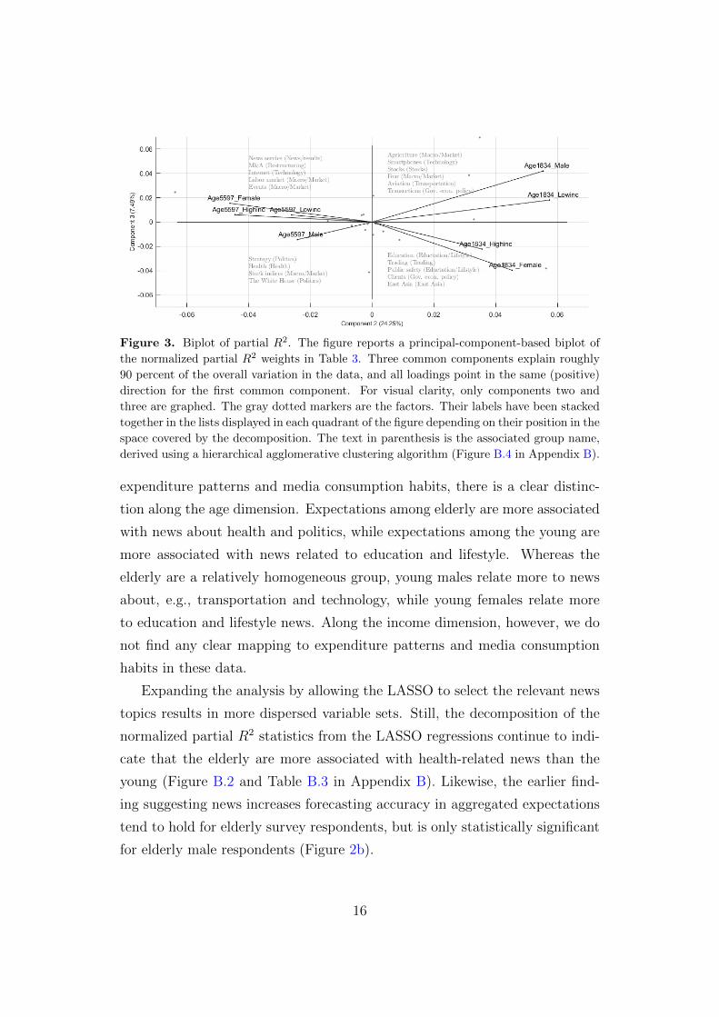
Figure 3. Biplot of partial R2. The figure reports a principal-component-based biplot of

the normalized partial R2 weights in Table 3. Three common components explain roughly

90 percent of the overall variation in the data, and all loadings point in the same (positive)

direction for the first common component. For visual clarity, only components two and

three are graphed. The gray dotted markers are the factors. Their labels have been stacked

together in the lists displayed in each quadrant of the figure depending on their position in the

space covered by the decomposition. The text in parenthesis is the associated group name,

derived using a hierarchical agglomerative clustering algorithm (Figure B.4 in Appendix B).

expenditure patterns and media consumption habits, there is a clear distinc-

tion along the age dimension. Expectations among elderly are more associated

with news about health and politics, while expectations among the young are

more associated with news related to education and lifestyle. Whereas the

elderly are a relatively homogeneous group, young males relate more to news

about, e.g., transportation and technology, while young females relate more

to education and lifestyle news. Along the income dimension, however, we do

not find any clear mapping to expenditure patterns and media consumption

habits in these data.

Expanding the analysis by allowing the LASSO to select the relevant news

topics results in more dispersed variable sets. Still, the decomposition of the

normalized partial R2 statistics from the LASSO regressions continue to indi-

cate that the elderly are more associated with health-related news than the

young (Figure B.2 and Table B.3 in Appendix B). Likewise, the earlier find-

ing suggesting news increases forecasting accuracy in aggregated expectations

tend to hold for elderly survey respondents, but is only statistically significant

for elderly male respondents (Figure 2b).

16

3 Information rigidities in theory

We now turn to address whether the degree of information rigidity among

households is state-dependent and a function of media coverage. To structure

the analysis, the easy to implement noisy information model suggested by

Coibion and Gorodnichenko (2015) is augmented with a simple reduced form

media channel.

We start by making the assumption that households do not follow infla-

tion as measured by the statistical agency per se, but get information about

future prices primarily through the media, which operate as information inter-

mediaries between agents and the state of the world (Nimark and Pitschner

(2019)). While this information object is high-dimensional, letting πNt denote

an aggregated measure of relevant media coverage, the signal agent i receives

about inflation at time period t is:

sit = πNt + ωit ωit ∼ N(0, σ2ωt), (2)

where ωit is idiosyncratic noise. The noise term captures differences in how

agents weigh and interpret different news sources and items, while the precision

of the signal is state-dependent.

News coverage has persistence, and the time series properties of media

coverage, as perceived by the agents, are modeled as an autoregressive process:

πNt = ρNt πNt−1 + νNt νNt ∼ N(0, σ2

νt), (3)

where ρNt and σ2νt depend on the time index t. Variation in ρNt can be due

to major economic or political events that become extensively covered by the

media, while a higher σ2νt implies that news reporting becomes less predictable,

e.g., in times of abrupt economic or political changes.

To link inflation to news about inflation, we build on the results presented

in the previous section and assume the media fulfills its purpose in informing

the public about important developments in society, and work with a tractable

17

and simple editorial function:

πNt = πt + αt, (4)

where αt is a time-fixed effect, capturing for example potential media biases.

Importantly, under the maintained assumption that agents do not follow infla-

tion per se, they are not in the position to bias-adjust the news signal towards

actual inflation. Likewise, combining (3) and (4) implies that agents’ perceived

time series properties of news are a composite of actual inflation developments

and time-fixed media effects. However, since agents’ have delegated their in-

formation choice to the media, they are not able to discriminate between these

two factors.5

As agents do not observe relevant news coverage directly (πNt ), but only

a noisy measure of it, the fundamental model feature is a signal extraction

problem. The agents use the Kalman filter for this purpose. Given (2) and

(3), the Kalman Gain is:

Kt = ρNt Ψt(Ψt + σ2ωt)−1, (5)

and captures the weight assigned to new information about πNt in the pre-

diction error (with variance Ψt). Averaging across agents, iterating h periods

forward, and using (4), gives:

πt+h − Ftπt+h = ct + βt(Ftπt+h − Ft−1πt+h) + et, (6)

where Ftπt+h is households’ expectation of future inflation, βt = 1−KtKt

, ct =

−αt+h, and et =∑h

j=1(ρNt )h−jνNt+j.

As in Coibion and Gorodnichenko (2015), equation (6) describes the rela-

5In general, these assumptions are consistent with Nimark and Pitschner (2019), who es-tablish optimality conditions for the delegated information choice mechanism, and they areconsistent with a substantial literature showing that people are not fully informed aboutimportant expenses (Chetty and Saez (2013), Jensen (2010), Carter and Milon (2005)).Moreover, most of the variation in household level inflation is disconnected from movementsin aggregate inflation (Kaplan and Schulhofer-Wohl (2017)), making it perfectly rational forhouseholds to not follow aggregate inflation directly, but rather use the news media for thispurpose.

18

tionship between ex-post forecast errors and ex-ante mean forecast revisions.

Although individuals form their forecasts rationally conditional on their in-

formation set, the ex-post mean forecast error across agents is systematically

predictable using ex-ante mean forecast revisions due to gradual adjustment

of beliefs to new information. A higher value of βt implies a higher degree of

information rigidity. Conversely, if βt = ct = 0, we have FIRE. The media

effect comes through (5). βt decreases if media persistence (ρNt ) is high and

increases if the amount of noise in the signal (σ2ωt) is high (relative to σ2

νt). In

contrast, in the conventional model, where agents are assumed to follow infla-

tion directly, the degree of information rigidity is determined by properties of

inflation itself.67

4 Information rigidities in the data

The theoretical predictions from the model in the previous section are tested

using a two-step estimation approach. In Section 4.1 (6) is used to estimate

βt, while we test if the underlying time series features of media coverage help

explain the evolution of βt, as predicted by (5), in Section 4.2.

4.1 Time-varying information rigidities?

The MSC survey only contains households’ forecast of inflation over the course

of the next year, resulting in non-overlapping time periods in observed forecast

revisions. For this reason, we follow Coibion and Gorodnichenko (2015), and

instrument the forecast revisions using the (log) change in the monthly price

of oil. In a time-varying parameter setting, however, a traditional instrumen-

tal variable (IV) estimator will still be biased due to the induced correlation

6Appendix F shows that this is also the case here if agents form an expectation about αt in(4). However, as documented in Section 4.3, using properties of inflation gives results atodds with theory, suggesting that this assumption is questionable.

7As noted by one referee, another plausible mechanism for assessing how the media affectsinformation rigidities is to assume news coverage provides noisy signals about inflation de-velopments directly. Although this line of reasoning does not map fully into the frameworkpresented above, it still captures the underlying idea, where information rigidity should belower in times of higher precision. Appendix G expands on this reasoning, and shows thatthe main conclusion presented below also holds under this alternative view.

19

between the time-varying parameters and the error term. This issue has often

been ignored in the literature (Chang-Jin et al. (2010)), but can be solved

using a control function approach. As described in Appendix H.1, this implies

the following system:

yt = ct + βtxt + γv∗t + wt wt ∼ i.i.d.N(0, σ2w) (7)

xt = δtzt + σvv∗t v∗t ∼ i.i.d.N(0, 1), (8)

where yt = πt+12,t+1 − Ftπt+12,t+1 and xt = Ftπt+12,t+1 − Ft−1πt+11,t denote

households’ forecast errors and revisions, respectively, of U.S. headline CPI

inflation over the next year, and zt is the instrument. v∗t = σ−1v (xt − ztδt) is

the control function, and the disturbance term wt is uncorrelated with xt and

βt conditional on v∗t .

To be faithful to the null hypothesis of full information, i.e., βt = 0, we

use the Latent Threshold Model (LTM) idea by Nakajima and West (2013) to

enforce dynamic sparsity on the system through the time-varying parameters.

For βt the LTM structure can be written as:

βt = β∗t ςβ,t ςβ,t = I(|β∗t | ≥ dβ) β∗t = β∗t−1 + υβ∗,t, (9)

where β∗t follows a random walk process, with υβ,t ∼ i.i.d.N(0, σ2β∗υ), and ςβ,t is

a zero one variable, whose value depends on the indicator function I(|β∗t | ≥ dβ).

If |β∗t | is above the the threshold value dβ, then ςβ,t = 1, otherwise ςβ,t = 0, and

βt shrinks to zero. For the ct parameter, a similar, but independent, structure

is assumed. For the δt parameter in (8), sparsity is not enforced. Doing so

would go against the standard IV relevance criterion. Instead, we let δt follow

a regular random walk process with error term υδ,t ∼ i.i.d.N(0, σ2δυ). Finally,

υβ∗,t , υc∗,t, and υδ,t are assumed to be independent of each other and wt and

v∗t .

Equations (7) and (8), together with the law-of-motion for ct, βt, and δt, are

used to estimate all the parameters of the model jointly in a state space system

using MCMC simulations. This avoids concerns about generated regressors in

two-stage approaches, and allows us to sample the model’s latent states jointly

20

with the hyper-parameters. In the interest of conserving space, details about

priors, initialization, and the estimation algorithm are relegated to Appendix

H.1. We note here, however, two points about the prior specification which

are particularly relevant in this setting. First, we set the prior variance for

σ2β∗υ equal to 0.22. This results in a roughly 95 percent prior probability of

a sevenfold cumulative change in β∗t over the sample length considered here,

which is well inside the range of low frequency change in information rigidity

documented in Coibion and Gorodnichenko (2015) for professional forecasters.8

Second, to obey the IV relevance criterion, we a priori allow for much less

variation in δt and set the prior variance of σ2δυ equal to 0.012 (and initialize δt

at the OLS solution).

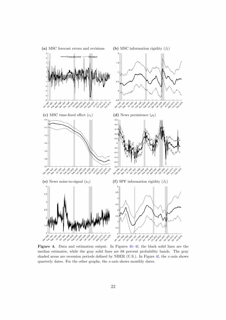
The MSC forecast errors and revisions are reported in Figure 4a, while the

time-varying posterior estimates of βt are reported in Figure 4b. Given that

we work in a high-dimensional time-varying parameter setting, the posterior

uncertainty in the βt estimate is naturally large. Still, three periods stand

out as having a particular high degree of information rigidity, namely the late

1990s, mid 2000s, and the financial crisis years.9

Interpreted through the lens of the model in Section 3, our estimates suggest

that the weight agents put on new information, i.e., Kt = 1/(1 + βt), varies

from roughly 0.7, during the early 1990s and prior to the Great Recession

period, to less than 0.5 during the financial crisis, with an average across the

sample of roughly 0.6. As discussed in Coibion and Gorodnichenko (2015),

information rigidity of this magnitude has profound macroeconomic effects in

theoretical models incorporating information frictions.

To bridge our analysis with the earlier literature, Figure 4f reports esti-

mates of (7) using quarterly SPF expectations, with details about estimation

relegated to Appendix H.1. Starting in the early 1990s, information rigidity

among professionals shares some of the same time-varying features as those

8This prior assumption only affects the cumulative change we might observe, not the timeevolution of the parameter itself. Our main results are fairly robust to other reasonableprior choices (Appendix H.1.3).

9Although not our primary focus, the ct parameter is negative and downward trending (Figure4c). This indicates that media biases are not constant across time, as also suggested byfindings in, e.g., Souleles (2004), and a full departure from FIRE.

21

(a) MSC forecast errors and revisions (b) MSC information rigidity (βt)

(c) MSC time-fixed effect (ct) (d) News persistence (ρt)

(e) News noise-to-signal (κt) (f) SPF information rigidity (βt)

Figure 4. Data and estimation output. In Figures 4b–4f, the black solid lines are the

median estimates, while the gray solid lines are 68 percent probability bands. The gray

shaded areas are recession periods defined by NBER (U.S.). In Figure 4f, the x-axis shows

quarterly dates. For the other graphs, the x-axis shows monthly dates.

22

obtained for households, and, as in Coibion and Gorodnichenko (2015), it also

contains an upward-drifting trend during this time period. Moreover, the time

series average of the series is well in line with constant parameter estimates

obtained in earlier studies, indicating that professionals only put roughly 40

percent weight on new relative to old information. This number is lower than

for households, which might be surprising. Still, an extensive evaluation of a

constant parameter version the model, for both MSC and SPF data, yields the

same conclusion (Tables B.4 and B.5 in Appendix B).

4.2 News-driven information rigidities?

To test whether the degree of information rigidity among households is a func-

tion of media coverage, as predicted by (5), we estimate:

βt = c+ γ1ρt + γ2κt + ut, (10)

where βt is the median time-varying information rigidity, reported in Figure 4b,

while ρt and κt are the persistence and noise-to-signal ratio in the underlying

information set S. S, ρt and κt are defined as follows:

First, we use the LASSO results from Section 2 to define S. At an abstract

level, the idea here is to construct an approximation to the high dimensional

object πNt in (2). Under the assumption that only news topics with predictive

power for expectations are relevant for describing the information households

care about, we use the set Se|FMD from Table 1 as our Benchmark selection.

Second, for each of the news topics i in S, we estimate time-varying autore-

gressive models, of order one, to obtain posterior draws of ρi,t and σi,t, i.e., the

time-varying persistence and volatility for news topic i. The model structure,

together with the Gibbs simulations used for estimation, is standard in the

time series literature and is described in greater detail in Appendix H.2. Next,

a measure of the noise in the signal, denoted ωi,t, is constructed using the sum

of the standard deviation in the posterior article weight distributions, and in

the articles selected to tone-adjust the news topic time series. Both estimates

are easily available from the topic model output. Intuitively, this noise measure

23

can be interpreted as follows: If it is difficult for the topic model algorithm to

classify the topic proportions of a given article with high precision, it would

likely be difficult for a human as well. Thus, uncertainty regarding what the

news is about increases. Likewise, uncertainty increases if articles differ in

terms of their tone.

Finally, aggregating across all the news topics i in the set S, and combining

the output from step two above, one obtains:

ρt =n∑i=1

$iρi,t κt =n∑i=1

$iκi,t with κi,t =ωi,tσi,t

and $i =R2i∑n

i=1R2i

, (11)

where $i is the normalized partial R2 statistic from the relevant regression in

Table 1. Thus, variables are weighted according to their relative importance

when constructing ρt and κt, while uncertainty in these estimates comes from

the posterior distribution of ρi,t and σi,t.

To control for the generated regressor issue, we use non-informative natural

conjugate priors and draw from (10) using the posterior estimates of ρt and

κt. Accordingly, the parameter estimates γ1 and γ2 are drawn from the OLS

solution, but taking into account the generated regressors issue by sampling

from the full distribution of ρt and κt (Bianchi et al. (2017)).

Figures 4d and 4e graphs the posterior distribution of the estimates in (11).

News persistence varies significantly across time and tends to be especially high

around recession periods. The noise-to-signal ratio displays a more surprising

pattern. It associates the mid 1990s as a particularly “noisy period” and

contains an upward-drifting trend starting around year 2000.10

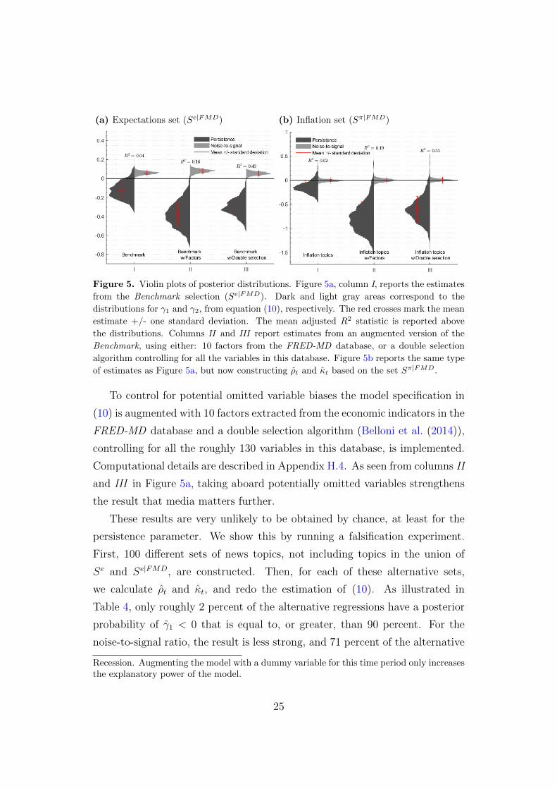
Column I in Figure 5a reports the results from estimating (10) using the

Benchmark selection. The time series properties of relevant topics help explain

the time-varying information rigidity among households, and the coefficient

estimates have the correct sign. A higher persistence and lower noise-to-signal

ratio lead to a reduction in information rigidity.11

10The method used to construct this variable is intuitive, but also somewhat sensitive to theraw corpus data. If some time periods contain news extracts from fewer, or different types,of articles, this might contaminate our noise-to-signal measure.

11Because the most important topics are the same in both sets, this result also holds whendefining S based on Se instead of Se|FMD. Likewise, this result is not driven by the Great

24

(a) Expectations set (Se|FMD) (b) Inflation set (Sπ|FMD)

Figure 5. Violin plots of posterior distributions. Figure 5a, column I, reports the estimates

from the Benchmark selection (Se|FMD). Dark and light gray areas correspond to the

distributions for γ1 and γ2, from equation (10), respectively. The red crosses mark the mean

estimate +/- one standard deviation. The mean adjusted R2 statistic is reported above

the distributions. Columns II and III report estimates from an augmented version of the

Benchmark, using either: 10 factors from the FRED-MD database, or a double selection

algorithm controlling for all the variables in this database. Figure 5b reports the same type

of estimates as Figure 5a, but now constructing ρt and κt based on the set Sπ|FMD.

To control for potential omitted variable biases the model specification in

(10) is augmented with 10 factors extracted from the economic indicators in the

FRED-MD database and a double selection algorithm (Belloni et al. (2014)),

controlling for all the roughly 130 variables in this database, is implemented.

Computational details are described in Appendix H.4. As seen from columns II

and III in Figure 5a, taking aboard potentially omitted variables strengthens

the result that media matters further.

These results are very unlikely to be obtained by chance, at least for the

persistence parameter. We show this by running a falsification experiment.

First, 100 different sets of news topics, not including topics in the union of

Se and Se|FMD, are constructed. Then, for each of these alternative sets,

we calculate ρt and κt, and redo the estimation of (10). As illustrated in

Table 4, only roughly 2 percent of the alternative regressions have a posterior

probability of γ1 < 0 that is equal to, or greater, than 90 percent. For the

noise-to-signal ratio, the result is less strong, and 71 percent of the alternative

Recession. Augmenting the model with a dummy variable for this time period only increasesthe explanatory power of the model.

25

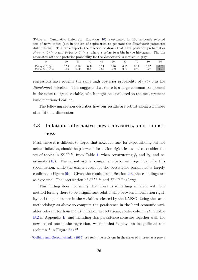
Table 4. Cumulative histogram. Equation (10) is estimated for 100 randomly selected

sets of news topics (not in the set of topics used to generate the Benchmark parameter

distributions). The table reports the fraction of draws that have posterior probabilities

Pr(γ1 < 0) ≥ x and Pr(γ2 > 0) ≥ x, where x refers to a bin in the histogram. The bin

associated with the posterior probability for the Benchmark is marked in gray.

x 10 20 30 40 50 60 70 80 90

Pr(γ1 < 0) ≥ x 0.54 0.48 0.34 0.24 0.20 0.15 0.11 0.07 0.02Pr(γ2 > 0) ≥ x 0.96 0.90 0.89 0.86 0.82 0.81 0.79 0.77 0.71

regressions have roughly the same high posterior probability of γ2 > 0 as the

Benchmark selection. This suggests that there is a large common component

in the noise-to-signal variable, which might be attributed to the measurement

issue mentioned earlier.

The following section describes how our results are robust along a number

of additional dimensions.

4.3 Inflation, alternative news measures, and robust-

ness

First, since it is difficult to argue that news relevant for expectations, but not

actual inflation, should help lower information rigidities, we also consider the

set of topics in Sπ|FMD, from Table 1, when constructing ρt and κt, and re-

estimate (10). The noise-to-signal component becomes insignificant for this

specification, while the earlier result for the persistence parameter is largely

confirmed (Figure 5b). Given the results from Section 2.3, these findings are

as expected. The intersection of Se|FMD and Sπ|FMD is large.

This finding does not imply that there is something inherent with our

method forcing there to be a significant relationship between information rigid-

ity and the persistence in the variables selected by the LASSO. Using the same

methodology as above to compute the persistence in the hard economic vari-

ables relevant for households’ inflation expectations, confer column II in Table

B.2 in Appendix B, and including this persistence measure together with the

news-based one in the regression, we find that it plays an insignificant role

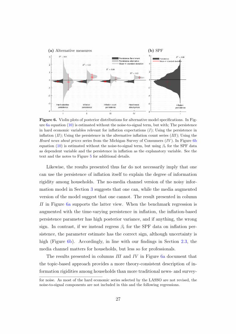
(column I in Figure 6a).12

12Coibion and Gorodnichenko (2015) use real-time revisions in the series of interest as a proxy

26

(a) Alternative measures (b) SPF

Figure 6. Violin plots of posterior distributions for alternative model specifications. In Fig-

ure 6a equation (10) is estimated without the noise-to-signal term, but with; The persistence

in hard economic variables relevant for inflation expectations (I ); Using the persistence in

inflation (II ); Using the persistence in the alternative inflation count series (III ); Using the

Heard news about prices series from the Michigan Survey of Consumers (IV ). In Figure 6b

equation (10) is estimated without the noise-to-signal term, but using βt for the SPF data

as dependent variable and the persistence in inflation as the explanatory variable. See the

text and the notes to Figure 5 for additional details.

Likewise, the results presented thus far do not necessarily imply that one

can use the persistence of inflation itself to explain the degree of information

rigidity among households. The no-media channel version of the noisy infor-

mation model in Section 3 suggests that one can, while the media augmented

version of the model suggest that one cannot. The result presented in column

II in Figure 6a supports the latter view. When the benchmark regression is

augmented with the time-varying persistence in inflation, the inflation-based

persistence parameter has high posterior variance, and if anything, the wrong

sign. In contrast, if we instead regress βt for the SPF data on inflation per-

sistence, the parameter estimate has the correct sign, although uncertainty is

high (Figure 6b). Accordingly, in line with our findings in Section 2.3, the

media channel matters for households, but less so for professionals.

The results presented in columns III and IV in Figure 6a document that

the topic-based approach provides a more theory-consistent description of in-

formation rigidities among households than more traditional news- and survey-

for noise. As most of the hard economic series selected by the LASSO are not revised, thenoise-to-signal components are not included in this and the following regressions.

27

based methods do; Regressing households’ information rigidity on the topic-

based persistence measure and the persistence in the alternative count-based

media measure (Section 2.2) results in an uncertain point estimate with the

wrong sign for the latter variable; Including the variable measuring if people

have heard news about prices from the MSC itself (Figure B.3 in Appendix

B) in the regression, we observe, as in Ehrmann et al. (2017), that it actually

increases information rigidities.

Finally, in the interest of conserving space, a detailed analysis using the

MSC micro-data is relegated to Appendix E. In short, information rigidity is

time-varying also among survey cohorts, at least when the level of aggregation

is not too low, and the relationship between information rigidities and relevant

media coverage described above largely holds.

5 Conclusion

Media’s role in the expectation formation process has received relatively little

attention in macroeconomics. Using a novel news topic-based approach, this

paper contributes by investigating the role of the media for inflation expecta-

tions and information rigidities among U.S. households. Taking the view that

the degree of information rigidity is state-dependent, and that the media act as

information intermediaries between agents and the state of the world, we find

empirical support for the following: First, the news types the media choose to

report on are good predictors of both inflation and inflation expectations, and

news coverage helps households form more accurate expectations. Second, in

a standard noisy information model, augmented with a simple media channel,

we document that the degree of information rigidity among households varies

across time, and that relevant media coverage helps explain this variation.

These results are robust to numerous alternative experiments and also largely

hold when analyzing the cross-sectional dimension of households’ expectations.

Thus, our analysis should be useful for future theoretical and empirical work

investigating media’s important role in the expectation formation process.

28

References

Armantier, O., S. Nelson, G. Topa, W. van der Klaauw, and B. Zafar (2016).

The Price Is Right: Updating Inflation Expectations in a Randomized Price

Information Experiment. The Review of Economics and Statistics 98 (3),

503–523.

Belloni, A. and V. Chernozhukov (2013). Least squares after model selection

in high-dimensional sparse models. Bernoulli 19 (2), 521 – 547.

Belloni, A., V. Chernozhukov, and C. Hansen (2014). High-dimensional meth-

ods and inference on structural and treatment effects. Journal of Economic

Perspectives 28 (2), 29–50.

Bianchi, D., M. Guidolin, and F. Ravazzolo (2017). Macroeconomic factors

strike back: A bayesian change-point model of time-varying risk exposures

and premia in the u.s. cross-section. Journal of Business & Economic Statis-

tics 35 (1), 110–129.

Blei, D. M., A. Y. Ng, and M. I. Jordan (2003). Latent Dirichlet Allocation.

J. Mach. Learn. Res. 3, 993–1022.

Blinder, A. S. and A. B. Krueger (2004). What does the public know about

economic policy, and how does it know it? Working Paper 10787, National

Bureau of Economic Research.

Carroll, C. D. (2003). Macroeconomic Expectations of Households and Profes-

sional Forecasters. The Quarterly Journal of Economics 118 (1), 269–298.

Carter, D. W. and J. W. Milon (2005). Price knowledge in household demand

for utility services. Land Economics 81 (2), 265–283.

Chang, J., S. Gerrish, C. Wang, J. L. Boyd-graber, and D. M. Blei (2009).

Reading tea leaves: How humans interpret topic models. In Y. Bengio,

D. Schuurmans, J. Lafferty, C. Williams, and A. Culotta (Eds.), Advances

in Neural Information Processing Systems 22, pp. 288–296. Cambridge, MA:

The MIT Press.

29

Chang-Jin, K. et al. (2010). Dealing with endogeneity in regression models

with dynamic coefficients. Foundations and Trends R© in Econometrics 3 (3),

165–266.

Chetty, R. and E. Saez (2013). Teaching the Tax Code: Earnings Responses to

an Experiment with EITC Recipients. American Economic Journal: Applied

Economics 5 (1), 1–31.

Coibion, O. and Y. Gorodnichenko (2012). What can survey forecasts tell us

about information rigidities? Journal of Political Economy 120 (1), 116–159.

Coibion, O. and Y. Gorodnichenko (2015). Information rigidity and the expec-

tations formation process: A simple framework and new facts. The American

Economic Review 105 (8), 2644–2678.

Coibion, O., Y. Gorodnichenko, and R. Kamdar (2018). The Formation of

Expectations, Inflation and the Phillips Curve. Journal of Economic Liter-

ature 56 (4), 1447–91.

Coibion, O., Y. Gorodnichenko, and M. Weber (2019). Monetary policy com-

munications and their effects on household inflation expectations. Technical

report, National Bureau of Economic Research.

Curtin, R. (2007). What US Consumers Know About Economic Conditions.

OECD.

Doms, M. and N. J. Morin (2004). Consumer sentiment, the economy, and

the news media. Finance and Economics Discussion Series 2004-51, Board

of Governors of the Federal Reserve System (US).

Dovern, J., U. Fritsche, P. Loungani, and N. Tamirisa (2015). Information

rigidities: Comparing average and individual forecasts for a large interna-

tional panel. International Journal of Forecasting 31 (1), 144–154.

Drager, L. and M. J. Lamla (2017). Imperfect information and consumer infla-

tion expectations: Evidence from microdata. Oxford Bulletin of Economics

and Statistics 79 (6), 933–968.

30

Ehrmann, M., D. Pfajfar, and E. Santoro (2017). Consumers’ Attitudes

and Their Inflation Expectations. International Journal of Central Bank-

ing 13 (1), 225–259.

Fullone, F., M. Gamba, E. Giovannini, and M. Malgarini (2007). What Do

Citizens Know about Statistics. OECD.

Gentzkow, M., J. M. Shapiro, and M. Sinkinson (2011). The effect of newspaper

entry and exit on electoral politics. American Economic Review 101 (7),

2980–3018.

Grossman, S. J. and J. E. Stiglitz (1980). On the impossibility of information-

ally efficient markets. The American Economic Review 70 (3), 393–408.

Jensen, R. (2010). The (perceived) returns to education and the demand for

schooling. The Quarterly Journal of Economics 125 (2), 515–548.

Kaplan, G. and S. Schulhofer-Wohl (2017). Inflation at the household level.

Journal of Monetary Economics 91 (C), 19–38.

King, G., B. Schneer, and A. White (2017). How the news media activate

public expression and influence national agendas. Science 358 (6364), 776–

780.

Lamla, M. J. and S. M. Lein (2014). The role of media for consumers’ inflation

expectation formation. Journal of Economic Behavior & Organization 106,

62 – 77.

Larsen, V. H. and L. A. Thorsrud (2019). The value of news for economic

developments. Journal of Econometrics 210 (1), 203–218.

Loungani, P., H. Stekler, and N. Tamirisa (2013). Information rigidity in

growth forecasts: Some cross-country evidence. International Journal of

Forecasting 29 (4), 605 – 621.

Mackowiak, B. and M. Wiederholt (2009). Optimal sticky prices under rational

inattention. The American Economic Review 99 (3), 769–803.

31

McCracken, M. W. and S. Ng (2016). FRED-MD: A Monthly Database for

Macroeconomic Research. Journal of Business & Economic Statistics 34 (4),

574–589.

Nakajima, J. and M. West (2013). Bayesian Analysis of Latent Threshold

Dynamic Models. Journal of Business & Economic Statistics 31 (2), 151–

164.

Nimark, K. P. and S. Pitschner (2019). News media and delegated information

choice. Journal of Economic Theory 181, 160 – 196.

Pfajfar, D. and E. Santoro (2013). News on Inflation and the Epidemiology

of Inflation Expectations. Journal of Money, Credit and Banking 45 (6),

1045–1067.

Prat, A. (2018). Media power. Journal of Political Economy 126 (4), 1747–

1783.

Shiller, R. J. (2017). Narrative economics. American Economic Review 107 (4),

967–1004.

Sims, C. A. (2003). Implications of rational inattention. Journal of Monetary

Economics 50 (3), 665 – 690.

Souleles, N. S. (2004). Expectations, heterogeneous forecast errors, and con-

sumption: Micro evidence from the michigan consumer sentiment surveys.

Journal of Money, Credit and Banking 36 (1), 39–72.

Thorsrud, L. A. (2018). Words are the new numbers: A newsy coincident index

of the business cycle. Journal of Business & Economic Statistics , 1–17.

Tibshirani, R. (1996). Regression shrinkage and selection via the lasso. Journal

of the Royal Statistical Society. Series B (Methodological) 58 (1), 267–288.

Woodford, M. (2009). Information-constrained state-dependent pricing. Jour-

nal of Monetary Economics 56 (S), 100–124.

32