Embed Size (px)
Citation preview
New York City Department of Environmental Protection Bureau of Water Supply
Upper Esopus Creek Watershed Turbidity/Suspended Sediment Monitoring Study: Project Design Report
First Submitted: January 31, 2017 Revised for Comment Resolution: July 31, 2017
Prepared in accordance with Section 2.3.6 of the NYCDEP
December 2016 Long-Term Watershed Protection Plan
Prepared by: DEP, Bureau of Water Supply

i
Foreword
This study design and associated QAPPs for monitoring and characterizing turbidity and suspended sediment sources in the Esopus Creek watershed and evaluating sediment and turbidity reduction projects in the Stony Clove Creek watershed was developed by the WLCP Stream Management Program Unit and the U.S. Geological Survey NYS Water Science Center. This is considered a complete and final document; however, the study design may be modified as the study progresses if additional methods, metrics, analytical techniques are identified as needed. The study design and associated QAPPS will be revised and redistributed.
Abbreviations and Acronyms
AWSMP Ashokan Watershed Stream Management Program CCEUC Cornell Cooperative Extension of Ulster County FAD Filtration Avoidance Determination GIS Geographic Information System LiDAR Light Detection and Ranging NHD National Hydrography Dataset NYSDEC New York City Department of Environmental Conservation NYCDEP New York City Department of Environmental Protection NYSDOH New York State Department of Health QAPP Quality Assurance Project Plans SFI Stream Feature Inventory SSC Suspended-sediment concentration SSL Suspended-sediment load SSY Suspended-sediment yield STRP Sediment and turbidity reduction project UCSWCD Ulster County Soil and Water Conservation District USEPA United States Environmental Protection Agency USGS United States Geological Survey
ii
Table of Contents 1.0 Introduction ........................................................................................................................................... 1
1.1 Background ....................................................................................................................................... 1
1.1.1 Study Area .................................................................................................................................. 2
1.1.2 Previous Studies ......................................................................................................................... 2
1.1.3 Previous STRPs .......................................................................................................................... 3
2.0 Study Goals and Objectives ................................................................................................................. 3
3.0 Methods .................................................................................................................................................. 4
3.1 Water Quality Sampling Design ...................................................................................................... 4
3.2 Suspended Sediment Source Characterization .............................................................................. 6
3.2.1 GIS and Hydraulic Analysis ...................................................................................................... 6
3.2.2 Geomorphic Investigations ........................................................................................................ 6
3.2.3 STRP Morphometric Monitoring ............................................................................................. 6
3.3 Study Variables and Analysis .......................................................................................................... 7
3.3.1 Water Quality Metrics ............................................................................................................... 7
3.3.2 Hydrology Metrics ..................................................................................................................... 7
3.3.3 Hydraulic Metrics ...................................................................................................................... 7
3.3.4 Geomorphology Metrics ............................................................................................................ 8
3.3.5 Management Practices Metrics ................................................................................................. 8
4.0 Data Management and Reporting ....................................................................................................... 8
5.0 References .............................................................................................................................................. 9
Tables ......................................................................................................................................................... 10
Figures ........................................................................................................................................................ 13
Appendices ................................................................................................................................................. 17
1
1.0 Introduction This technical report describes the research-based approach to improve understanding of turbidity generation in the Ashokan watershed and to evaluate the effectiveness of stream management practices to meaningfully reduce turbidity over a range of hydrologic, spatial and temporal scales. There are two Quality Assurance Project Plans (QAPPs) attached to this report that provide the details on the study design and quality control measures. This report and the associated QAPPs were revised in July 2017 to address comments provided by NYSDOH.
New York City Department of Environmental Protection (DEP) in collaboration with the U.S. Geological Survey (USGS), and support from the Ashokan Watershed Stream Management Program (AWSMP) partners – Ulster County Soil and Water Conservation District (UCSWCD) and Cornell Cooperative Extension of Ulster County (CCEUC) – will integrate a set of research, assessment, monitoring and treatment practice activities into a study framework. The study period is 11 years, starting data collection in Fall 2016 and continuing data collection through Fall 2026 with a final report in 2027. This study is designed to address three areas of research that will inform DEP’s mission to protect and improve source water quality:
• Continued characterization of how Esopus Creek sub-basins vary in terms of suspended sediment yield/turbidity. How do these differences change under a range of flow conditions and over time? How can characterization of this variability inform stream management strategies?
• Characterize how different stream reaches vary in terms of suspended sediment yield/turbidity within a specific sub-basin. What are the reach-level conditions and processes that lead to those heterogeneous yields?
• Utilizing the reach-level suspended sediment yield/turbidity characterization, evaluate the effectiveness of strategically located stream restoration projects designed to reduce turbidity. To what extent can suspended sediment yield/turbidity associated with these sources, channel conditions and processes be sustainably managed within the stream system?
1.1 Background The New York City water supply system provides more than 9 million people with clean drinking water each day from the world’s largest unfiltered water supply system. DEP is the agency responsible for the operation and protection of the water supply. Suspended-sediment concentrations (SSCs) and turbidity are primary water-quality concerns in the Ashokan Reservoir, which is part of the New York City water supply system in the Catskill Mountains of New York State (Figure 1). The upper Esopus Creek is the primary tributary to the Ashokan Reservoir. High magnitude storm flows in the Esopus Creek watershed carry high concentrations of suspended sediment entrained from alluvial and glacial sources within the stream channel network. The result is the delivery of highly turbid water to the Ashokan Reservoir. Once turbidity of Ashokan Reservoir water in the Catskill Aqueduct exceeds 10 NTU, DEP policy requires operational changes and possibly alum treatment of the NYC West-of-Hudson water supply to avoid exceeding the regulatory threshold of 5 NTU at the Kensico Reservoir intake. As part of the revised 2007 Filtration Avoidance Determination (FAD) DEP is
2
required to implement stream restoration projects in the Ashokan watershed designed to reduce turbidity. DEP is also required to conduct water quality monitoring studies that help identify turbidity source distribution and to evaluate the effectiveness of the turbidity reduction stream restoration projects.
In November 2014 DEP proposed a monitoring and research approach to (a) further guide understanding of the spatial and temporal distribution of suspended sediment loading/turbidity in the upper Esopus Creek watershed, (b) improve identification of the suspended sediment source loading within the Stony Clove Creek watershed, (c) use currently available data to provide an interim evaluation of the efficacy of turbidity reduction attributed to a set of projects constructed in the Stony Clove Creek watershed and (d) evaluate the effectiveness of stream restoration practices on reducing turbidity at the reach and sub-basin scale with sufficient pre- and post-construction water quality and geomorphic monitoring.
1.1.1 Study Area The upper Esopus Creek is located in the Catskill Mountains of New York State. In 1915, damming of a portion of the creek formed the Ashokan Reservoir splitting the creek into upper (upstream of the reservoir) and lower (downstream of the reservoir) segments. The Ashokan Reservoir watershed is 255 square miles and is one of two reservoirs in the New York City Catskill Reservoir System and one of six reservoirs in the West-of-Hudson Catskill-Delaware system. The upper Esopus Creek drains approximately 192 square miles of mostly forested mountainous terrain. The stream originates at Winnisook Lake at an elevation of 2,660 feet above sea level, and over the course of 26 miles descends to the Ashokan Reservoir at an elevation of 585 feet above sea level.
1.1.2 Previous Studies From 2010 to 2012, suspended-sediment concentrations (SSCs) and turbidity were measured at 14 monitoring sites throughout the upper Esopus Creek watershed to quantify SSC and turbidity levels, to estimate suspended-sediment loads (SSL) within the upper Esopus Creek watershed, and to investigate the relations between SSC and turbidity (McHale & Siemion, 2014). In situ turbidity probes provide a good surrogate for SSC and allowed for more accurate calculations of SSL than discrete suspended-sediment samples alone.
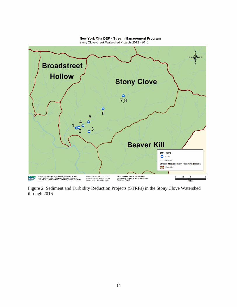
During the 2010-2012 study, the largest tributary, Stony Clove Creek, consistently produced higher SSCs and turbidity than any of the other Esopus Creek tributaries. The rest of the tributaries fell into two groups: those that produced moderate SSCs and turbidity, and those that produced low SSCs and turbidity. Within those two groups the tributary that produced the highest SSCs and turbidity varied from year to year depending on the hydrologic conditions within each tributary watershed. Within the Stony Clove Creek watershed several bank failures and hill slope mass failures in contact with the stream have exposed glacial and glacial lacustrine sediments creating a chronic source of suspended sediment and turbidity to Stony Clove Creek. Starting in 2001, DEP and Ulster and Greene County SWCDs began to address this problem by cataloging stream bank erosion, slope failures, exposed geology and collecting other geomorphic data to create stream feature inventories for the watershed. The geomorphic assessments have been used to identify priority stream reaches for stream stability restoration and/or hill slope stabilization projects intended to reduce reach sale production of turbidity. Eight suspended sediment and turbidity reduction projects (STRPs) were completed between 2012 and 2016
3
(Figure 2). This 10-year study will test the hypothesis that longitudinal water quality monitoring could help to identify stream sections that contribute disproportionately to turbidity levels and suspended sediment load in the watershed. Identifying those problem sections will in turn improve potential STRP site identification and prioritization as well as evaluation of STRP effectiveness at reducing turbidity levels and suspended sediment loads.
1.1.3 Previous STRPs The 8 STRPs that were completed within the Stony Clove watershed were:
1) Stony Clove Creek at Chichester Site 1 (2012);
2) Stony Clove Creek at Chichester Site 2-3 (2013);
3) Warner Creek Site 5 (2013);
4) Stony Clove-Warner Creek Confluence (2014);
5) Stony Clove Creek at Stony Clove Lane (2014);
6) Stony Clove Creek at Lanesville (2006; 2015);
7) Stony Clove Creek at Wright Road (2015); and
8) Stony Clove Creek Hill Slope Stabilization at Wright Road (2016).
Upstream/downstream and limited before/after turbidity and SSC monitoring sites were installed for many of these projects. Though the recorded flows at the Stony Clove Creek below Ox Clove near Chichester gage (01362370) have exceeded bankfull streamflow only once since project construction started in 2012, there has been a measureable reduction in turbidity levels and SSCs for the range in flows experienced since the projects were installed (Siemion, McHale, & Davis, 2016). This 10-year study should enable a greater range of flows to be monitored for STRP evaluation.
2.0 Study Goals and Objectives The goals of this study are to improve basin to reach-scale suspended sediment source characterization and to evaluate STRP effectiveness in reducing turbidity. The objectives of this study are broken into two categories, those necessary to characterize sources of suspended sediment and turbidity associated with changes in hydrology and differences in stream channel source conditions in the upper Esopus Creek watershed; and those specific to the detailed stream reach and STRP monitoring in the Stony Clove Creek watershed.
Upper Esopus Creek monitoring objectives:
1. Monitor SSC and turbidity levels through a range in discharge at three main stem locations and five tributaries within the upper Esopus Creek watershed and monitor turbidity levels only at an additional two tributaries.
2. Develop sediment and/or turbidity (dependent on the variables measured at each station) discharge rating curves for each monitoring location.
4
3. Estimate suspended sediment loads and yields at eight locations within the upper Esopus Creek watershed
4. Evaluate how changes in discharge affect SSC and turbidity and examine the relation between SSC and turbidity levels, stream feature inventories.
5. Evaluate the effectiveness of stream stability restoration projects implemented in the basin at reducing suspended sediment and turbidity.
Stony Clove Creek monitoring objectives:
1. Monitor and characterize the variability of SSC and turbidity levels among several stream reaches within the Stony Clove watershed using twenty monitoring stations.
2. Evaluate the effectiveness of STRPs using the reach-level suspended sediment and turbidity characterization.
3.0 Methods The details for field sampling methods, equipment used, data analysis and quality assurance measures are provided in the QAPPs attached to this report. The water quality monitoring and data analysis will be performed by USGS in accordance with the enclosed QAPP for Turbidity and Suspended Sediment Monitoring in the Upper Esopus Creek Watershed, Ulster County, NY (Appendix A). The study design includes sediment source characterization through geomorphic assessments and monitoring that will be primarily performed by DEP and AWSMP personnel in accordance with the enclosed QAPP for Turbidity and Suspended Sediment Source Characterization in the Upper Esopus Creek Watershed (Appendix B). Geomorphic monitoring also includes the monitoring of STRPs in accordance with stream disturbance permit monitoring requirements and program goals (Appendix C).
This section outlines the water quality sampling design, suspended sediment source characterization, and STRP monitoring methods which serve as the principal data acquisition components in this study, identifies the study variables and associated metrics used in the study, and discusses the data management, analysis and reporting.
3.1 Water Quality Sampling Design This is primarily a water quality monitoring-based study focused on turbidity and suspended sediment with supplemental geomorphic assessment and monitoring. USGS will lead the water quality sampling and analysis. The study uses a combination of three statistical sampling designs. The details for the turbidity and suspended sediment sampling methods and quality assurance/control measures are detailed in Appendix A.
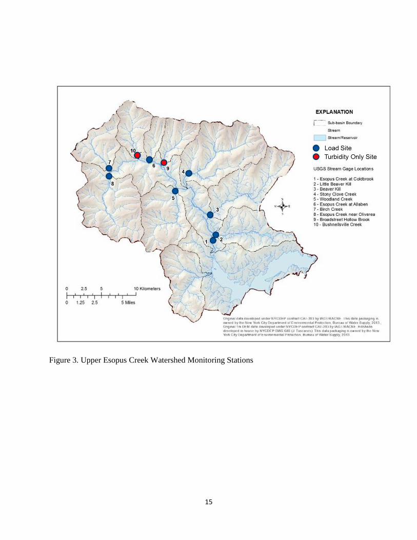
• Trend monitoring – measuring streamflow, turbidity and SSC and computing SSL in the Upper Esopus Creek watershed for 10 years at eight sub-basin monitoring stations and turbidity alone at two additional sub-basin monitoring stations (Table 1; Figure 3). Streamflow and turbidity will be reported for 15-minute intervals and SSC for discrete and equal discharge increment samples. Discrete samples will be collected throughout the range in streamflow and during each season. The discrete samples will be collected by automated sampling equipment that is triggered to sample based on pre-determined
5
changes in stage and/or turbidity during storms. Equal width –depth integrated and equal discharge-depth integrated samples will also be collected throughout the range in streamflow and during each season. SSC will also be derived from a turbidity-SSC regression equation at a 15-minute time step. Daily mean streamflow, turbidity, and SSC will be derived from the 15-minute values. This monitoring will be used to calculate sub-basin to basin suspended sediment yields (SSY) and to establish and/or revise suspended sediment and turbidity discharge rating curves for the Esopus Creek watershed and for segments of Esopus Creek and the primary tributary streams. Stream hydrology will be the primary predictor variable for turbidity and SSC. Separate geomorphic assessment and monitoring efforts in the monitored sub-basins will be used to identify potential geomorphic predictor variables that can help account for differences between the monitored sub-basins.
• Watershed before/after – measuring streamflow, turbidity and SSC at two long-term sub-basin “outlet” monitoring stations: (1) the Stony Clove Creek below Ox Clove at Chichester NY gage (0136270) and (2) the Esopus Creek at Coldbrook NY gage (01362500). The study period monitoring data will be used in conjunction with past monitoring data to evaluate the potential cumulative impact of suspended sediment and turbidity reduction projects (STRPs) in the Stony Clove watershed on turbidity, SSL and SSY at the sub-basin scale (Stony Clove) and basin scale (Esopus Creek). Tests for potential changes in suspended sediment concentrations and/or turbidity before/after sediment and turbidity reduction projects are completed using previously published methods given in Siemion and others, 2016, and Jastram and others, 2015. An analysis of covariance (ANCOVA) will be used to test for changes in the streamflow-SSC and streamflow-turbidity relations before/after sediment and turbidity reduction projects are completed. The SSC or turbidity will be used as the dependent variable, and streamflow as the independent variable. A STRP factor, used to separate the dataset into periods before and after construction of the STRP, will be used as the ANCOVA analysis factor. A significant difference in the STRP factor before and after STRP construction indicates a change in the relation between SSC or turbidity and streamflow. The nonparametric Wilcoxon rank sum test (Helsel and Hirsch, 2002) will be used to determine if significant (alpha equals 0.05) differences in SSC are measured between the before and after STRP construction periods at each streamgage at similar streamflow and to determine if significant differences in streamflow exist between periods. This analysis will target 10-percentile ranges in streamflow to reflect low, moderate, and high streamflows. Low streamflows are considered to be those that are equaled or exceeded 90 percent of the time (Q90). Moderate streamflows those that are equaled or exceeded between 45 and 55 percent of the time (Q45 to Q55). High streamflows those that are equaled or exceeded less than 10 percent of the time (Q10).
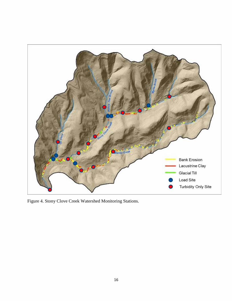
• Watershed above/below – measuring streamflow, turbidity and SSC and computing SSL at six monitoring stations and measuring only turbidity at 14 other locations in the Stony Clove Creek watershed to segment the stream network into discrete reaches and associated sub-basins (Table 2; Figure 4). This monitoring serves three primary purposes: (1) It will be used to establish and/or revise suspended sediment and turbidity discharge
6
rating curves for monitored segments of Stony Clove watershed streams. Stream hydrology will be the primary predictor variable for turbidity and SSC. Separate geomorphic assessment and monitoring efforts in the Stony Clove watershed will be used to identify potential geomorphic predictor variables that can account for differences between the monitored segments. (2) It will be used to prioritize three future STRP locations by identifying monitored stream segments that contribute measurable increases in SSL and turbidity. (3) It will be used to evaluate the potential efficacy of the proposed STRPs on reducing suspended sediment and turbidity at the monitored stream reach to segment scale.
3.2 Suspended Sediment Source Characterization This study starts with the assumption that the stream channel corridor is the principle source terrain for stream turbidity and suspended sediment, therefore source characterization will focus on stream channel process, physical condition, and material composition. DEP with support from AWSMP will lead the effort in obtaining (1) GIS and hydraulic analysis of conditions that may influence reach scale erosion risk hazard and suspended sediment yield and (2) sediment source characterization data using field-based fluvial geomorphology assessments/monitoring.
3.2.1 GIS and Hydraulic Analysis Rates of streambank erosion and meander migration have been successfully correlated with stream power (Knighton, 1998). Total and specific stream power will be tested as potential explanatory variables for the observed downstream changes in turbidity and suspended sediment concentration for given flow conditions. The 1-meter resolution digital elevation model and NHD hydrography developed from 2009 LiDAR data and flood frequency regional regression relationships developed by USGS can be used to derive the hydraulic parameters total and specific stream power for monitored reaches. The detail on stream power derivation is provided in Appendix B. Additional GIS-derived potential explanatory variables for turbidity and suspended sediment concentration will be examined and evaluated for potential inclusion in the study design. If additional variables are selected the study design will be modified to include them.
3.2.2 Geomorphic Investigations Characterizing stream channel geology, streambank erosion, streambed incision, hillslope mass failure, and stream bank material composition will be primarily through field work. The field-based assessments include mapping stream channel geology and sediment entrainment sites (stream bed incision, stream bank erosion and mass failure) using the Stream Feature Inventory (SFI) methods developed by DEP, periodic repeat topographic surveys of representative bank erosion monitoring sites, and sediment sampling for particle size distribution analysis. Appendix B provides the Quality Assurance Project Plan for the sediment source characterization methods that will be used in this study.
3.2.3 STRP Morphometric Monitoring Physical monitoring of STRPs is intended to measure the project’s performance in achieving stream stability through topographic surveying of stream channel cross sections and longitudinal profiles, stream bed material characterization through pebble counts and photographic monitoring. All morphometric monitoring results will be included in reviewing turbidity and suspended sediment monitoring data. UCSWCD staff are responsible for monitoring all stream
7
restoration projects for to up to 2-5 years following construction as specified in permits. All the constructed and future STRPs evaluated in this study are required to be monitored as detailed in Appendix C. DEP plans to have each STRP monitored beyond the period requirements of the project permits.
3.3 Study Variables and Analysis Table 3 presents the selected response (water quality parameters) and potential predictor (hydrologic, hydraulic, geomorphic, geologic) variables for this study. The two QAPPs attached to this study design report (Appendices A and B) explain each variable and the methods and quality controls for data collection to derive the variables. Turbidity, SSC, and SSL are considered response variables in this study. The potential explanatory variables that are assumed to influence turbidity, SSC, and SSL are derived from hydrological data, simplified spatial hydraulic analysis, geomorphologic investigations, and STRP implementation. It is assumed that not all potential explanatory variables are included in this study. Since the primary objectives of this analysis with respect to meeting the FAD objectives are basin scale source characterization (the upper Esopus Creek Watershed monitoring effort) and STRP efficacy evaluation (Stony Clove Watershed monitoring effort) the study is intentionally optimized to collect and analyze potential explanatory data that is consistent with the existing stream diagnostic assessment efforts of DEP and AWSMP. Additional variables and analytical techniques will be considered during the first two years with some potential pilot efforts to evaluate the efficiency in methods and potential value in analytical results.
3.3.1 Water Quality Metrics Measurements of turbidity and SSC will be reported for each monitoring station. Where SSC is not directly measured turbidity-SSC regression relationships will be used to provide estimated SSC values. Appendix A details the analytical methods for deriving SSL from the SSC and discharge data.
3.3.2 Hydrology Metrics Daily and instantaneous discharge values used to compute flow statistics (daily mean, peak flow magnitude-frequency, flow duration) are derived from stage-discharge ratings based on standard USGS methods detailed in Appendix A. Flood flow frequency is determined using the standard Log-Pearson Type III distribution analytical technique (Interagency Advisory Committee on Water Data, 1982). Peak flow turbidity, SSC and SSL will be associated with peak flow magnitude-frequency (recurrence interval value, e.g. 10-year flood) to evaluate role of discharge magnitude in measured water quality metrics for the upper Esopus Creek watershed and the Stony Clove watershed monitoring efforts. For the Stony Clove watershed analysis this can help identify the threshold stream flow magnitude values that transition from reach-scale SSL significance to basin scale. STRPs are assumed to be most effective for flows that have distinct and measurable reach-scale sediment loading; however, the threshold for those flows is currently unknown.
3.3.3 Hydraulic Metrics The only hydraulic variable that is currently considered for use as a potential explanatory variable is reach-scale stream power derived from reach slope and measured or estimated discharge magnitude. Work by others has shown that stream power (both total stream power and specific (or unit) stream power which factors in stream channel dimensions) is a valid predictive
8
variable for geomorphic stream channel response to hydrology (Knighton, 1998; Magilligan, Buraas, & Renshaw, 2015; Parker, Thorne, & Clifford, 2015). The study will explore various ways to examine the role of stream power as a possible metric for predicting turbidity and SSC induced through increased potential for stream erosion. Of course, actual turbidity and SSC are more dependent on stream channel geomorphology and geology; however, stream power may be useful in assessing whether a given reach with the geologic and geomorphic potential for turbidity and SSC will generate suspended sediment/turbidity.
3.3.4 Geomorphology Metrics This study will evaluate the role of stream bank erosion and stream channel incision in spatial differences in monitored turbidity and suspended sediment. There are several potential metrics that can be developed from mapping stream bank erosion. The simplest approach is to account for the presence of stream bank erosional processes in a monitored basin or reach. Reporting the percentage of linear active stream bank erosion for the total length of stream bank (sum of both banks) in the monitored stream is one way to account for lateral erosional process as a potential predictive metric. This can be further evaluated by stratifying the stream bank erosion into banks that are eroded primarily through hydraulic erosion versus those that are primarily through geotechnical mass failures. GIS and SFI mapping can also identify the percentage of the stream that is in erosive and non-erosive contact with hill slopes that would be prone to mass wasting sediment production. Similarly, differences in stream bank material composition can be accounted for as potential predictive metrics. In this study we will identify if the eroding stream bank is entirely composed of primarily coarse-grained, unconsolidated alluvium or contains non-alluvial sources of fine sediment such as glacial till, glacio-lacustrine sediment, or clay-enriched colluvium. The QAPP in Appendix B describes the primary sedimentologic units that will be accounted for in mapping stream bank erosion.
3.3.5 Management Practices Metrics In addition to the two water quality sampling design approaches to evaluating the potential effectiveness of STRPs in reducing measured turbidity and SSC (single watershed before/after; and above/below) we can also report a simple metric that represents the percentage of the monitored basin or stream reach that has removed stream channel contact with fine sediment sources as an additional means of evaluating the relative role of future STRPs in monitored reaches.
4.0 Data Management and Reporting The QAPPs attached to this Study Design Report (Appendices A and B) provide detail on the separate USGS and DEP data management practices, quality objective criteria and methods to achieve the quality objectives.
Coordination and collaboration of project partners (DEP, USGS and AWSMP) will be achieved through periodic reporting, quarterly to semi-annual project status meetings, and annual project planning. As part of DEP’s Long-Term Watershed Protection Plan, DEP will also prepare biennial status reports on preliminary/provisional study findings commencing in March 2019. A report on the first five years of study findings will be completed by November 30, 2022. The final report for the 10 years of water quality monitoring is scheduled for November 30, 2027.
9
5.0 References
Interagency Advisory Committee on Water Data. (1982). Guidelines for determining floodflow frequency: Hydrology Subcommittee Bulletin 17B. Reston, Va.: U.S. Geological Survey.
Knighton, D. (1998). Fluvial Forms and Processes: A New Perspective. London: Oxford University Press.
Magilligan, F. J., Buraas, E. M., & Renshaw, C. (2015). The efficacy of stream power and flow duration on geomorphic responses to catastrophic flooding. Geomorphology, 228, 175-188. doi:10.1016/j.geomorph.2014.08.016
McHale, M. R., & Siemion, J. (2014). Turbidity and suspended sediment in the upper Esopus Creek watershed, Ulster County, NY. U.S. Geological Survey Scientific INvestigations Report 2014-5200. doi:http://dx/doi.org/10.3133.sir20145200
Parker, C., Thorne, C. R., & Clifford, N. J. (2015). Development of ST:REAM: A reach-based stream power balance approach for predicting alluvial river channel adjustment. Earth Surface Processes and Landforms, 40(3), 403-413. doi:10.1002/esp.3641
Siemion, J., McHale, M. R., & Davis, W. D. (2016). Suspended-sediment and turbidity responses to sediment and turbidity reduction projects in the Beaver Kill, Stony Clove Creek and Warner Creek Watersheds, NY. U.S. Geological Survey Scientific Investigations Report 2016-5157. doi:https://doi.org/10.3133/sir20165157
10
Tables
Table 1. Upper Esopus Creek Sub-basin monitoring sites listed from upstream to downstream.
Site Name USGS Station ID
Site Type Measurements
1 Esopus Creek blw Lost Clove @ Big Indian NY 0136219503 Primary Streamflow, SSC, Turbidity,
Water Temperature
2 Birch Creek at Big Indian1 013621955 Primary Streamflow, SSC, Turbidity, Water Temperature
3 Bushnellsville Creek at Shandaken 01362197 Secondary Estimated Streamflow, Turbidity,
Water Temperature
4 Esopus Creek at Allaben1 01362200 Primary Streamflow, SSC, Turbidity, Water Temperature
5 Broad Street Hollow Brook at Allaben 01362232 Secondary Estimated Streamflow, Turbidity,
Water Temperature
6 Woodland Creek at Phonecia1 0136230002 Primary Streamflow, SSC, Turbidity, Water Temperature
7 Stony Clove Creek at Chichester1 01362370 Primary Streamflow, SSC, Turbidity,
Water Temperature
8 Beaver Kill at Mt. Tremper2 01362487 Primary Streamflow, SSC, Turbidity, Water Temperature
9 Little Beaver Kill at Beechford1 01362497 Primary Streamflow, SSC, Turbidity,
Water Temperature
10 Esopus Creek at Coldbrook1 01362500 Primary Streamflow, SSC, Turbidity, Water Temperature
1Existing streamflow site, 2Existing monitoring station funding ends September 30, 2015
11
Table 2. Stony Clove Creek Watershed Monitoring sites listed from upstream to downstream.
Site Name USGS Station ID
Station Type Measurements
1 Stony Clove Cr @ Edgewood NY 01362312 Secondary Estimated streamflow*, Turbidity 2 Myrtle Br abv Mouth @ Rt 214 @
Edgewood NY 01362322 Primary Streamflow, SSC, SSL, Turbidity
3 Stony Clove Creek above Wright Rd3 01362330 Secondary Estimated streamflow, Turbidity
4 Stony Clove Creek @ Wright Rd 01362332 Secondary Estimated streamflow, Turbidity 5 Stony Clove Cr @ Jansen Rd @
Lanesville NY 01362336 Primary Streamflow, SSC, SSL, Turbidity
6 Hollow Tree Br @ Rt214 @ Lanesville NY 01362345 Primary Estimated streamflow, SSC, SSL,
Turbidity 7 Hollow Tree Brook @
Lanesville2 01362342 Secondary Streamflow, Turbidity
8 Stony Clove Cr @ Lanesville NY 01362347 Secondary Estimated streamflow, Turbidity 9 Stony Clove Cr abv Moggre Rd nr
Chichester NY 01362349 Secondary Estimated streamflow, Turbidity
10 Stony Clove Creek @ Stony Clove Ln 01362350 Secondary Estimated streamflow, Turbidity
11 Warner Cr blw Silver Hollow Notch nr Edgewood NY 01362354 Secondary Estimated streamflow*, Turbidity
12 Warner Cr nr Carl Mountain nr Chichester NY 0136235575 Secondary Estimated streamflow*, Turbidity
13 Warner Cr in Silver Hollow nr Chichester NY 0136235580 Secondary Estimated streamflow, Turbidity
14 Warner Creek @ Silver Hollow Rd Bridge 01362356 Secondary Estimated streamflow, Turbidity
15 Warner Creek near Chichester 01362357 Primary Streamflow, SSC, SSL, Turbidity 16 Stony Clove Cr @ Chichester NY 01362359 Secondary Estimated streamflow, Turbidity 17 Ox Clove @ Chichester NY 01362365 Secondary Streamflow, Turbidity 18 Ox Clove abv mouth @
Chichester NY 01362368 Primary Estimated streamflow, SSC, SSL, Turbidity
19 Stony Clove Creek @ Chichester1 01362370 Primary Streamflow, SSC, SSL, Turbidity 20 Stony Clove Creek @ Phoenicia 01362398 Secondary Estimated streamflow, Turbidity
1Existing streamflow, SSC, SSL, turbidity site funded through separate DEP-USGS agreement, 2Existing streamflow site funded through separate DEP-USGS agreement, *6 streamflow measurements annually for estimation/calibration.
12
Table 3. List of Study Analytical Variables.
Variable Metrics Methods1 QAPP
PI
Water Quality Turbidity daily and runoff event mean value
(FNU) WQ A USGS
Suspended Sediment Concentration
daily and runoff event mean value (mg/L)
WQ A USGS
Suspended Sediment Load runoff event and annual value (ton) WQ, Q A USGS
Hydrology
Discharge (Daily, Storm) Mean, instantaneous peak, and duration analysis (cfs)
Q A USGS
Discharge Magnitude-Frequency
Return Period (yr) Q A USGS
Hydraulics
Stream Energy Stream power (W m-1), Unit stream power (W m-2)
H, C, G B DEP
Geomorphology
Drainage Area Drainage area (mi2) G B DEP
Erosional Process % Active Bank Hydraulic Erosion C B DEP
% Active Bank Mass Failure C B DEP
Presence of active headcuts (y/n) C B DEP
Channel/Hillslope Interaction
% Channel Contact with Hillslope Processes
G, C B DEP
Geology
Stream Bank Sediment Composition
% Erosional Contact Non-Alluvial Source Fine Sediment
C, S B DEP
% Erosional Contact w/ Alluvial Source Fine Sediment
C, S B DEP
Management Practices
STRP Implementation % Erosional contact with fine sediment mitigated
C, G B DEP
1 Methods: WQ = water quality monitoring; Q = stream discharge monitoring; H = hydraulic modeling; C = channel corridor assessment; G = GIS; S = sediment particle size analysis
13
Figures
Figure 1. Study Area
14
Figure 2. Sediment and Turbidity Reduction Projects (STRPs) in the Stony Clove Watershed through 2016
15
Figure 3. Upper Esopus Creek Watershed Monitoring Stations
16
Figure 4. Stony Clove Creek Watershed Monitoring Stations.

17
Appendices

Appendix A:
Quality Assurance Project Plan for Turbidity and Suspended Sediment Monitoring
in the Upper Esopus Creek Watershed, Ulster County, NY.
United States Geological Survey,
January 31, 2017
i
Quality Assurance Project Plan
for
Turbidity and Suspended Sediment Monitoring in the Upper
Esopus Creek Watershed, Ulster County, NY
Prepared by:
U.S. Geological Survey
New York Water Science Center
425 Jordan Road
Troy, NY 12180
Submitted
January 30, 2017
Revised:
July 24, 2017
i
APPROVAL SHEET
New York City Department of Environmental Protection
U.S. Geological Survey Project Managers:
Jason Siemion, Physical Scientist,
New York Water Science Center, Troy, NY, 518-285-5623
____________________________________________
Signature Date
Michael R. McHale, Research Hydrologist,
New York Water Science Center, Troy, NY, 518-285-5675
____________________________________________
Signature Date
ii
TABLE OF CONTENTS
APPROVAL SHEET ......................................................................................................................................................i
TABLE OF CONTENTS ............................................................................................................................................. ii
DISTRIBUTION LIST .................................................................................................................................................. 1
PROJECT MANAGEMENT......................................................................................................................................... 2
Project/Task Organization ......................................................................................................................................... 2
Project Organizational Chart ..................................................................................................................................... 3
Problem Definition/Background ................................................................................................................................ 4
Project/Task Description ........................................................................................................................................... 7
Quality Objectives and Criteria ............................................................................................................................... 11
Special Training/Certification.................................................................................................................................. 11
Documents and Records .......................................................................................................................................... 11
DATA GENERATION AND ACQUISITION ........................................................................................................... 12
Experimental Design ............................................................................................................................................... 12
Sampling Methods ................................................................................................................................................... 13
Sample Handling and Custody ................................................................................................................................ 13
Analytical Methods .................................................................................................................................................. 13
Quality Control ........................................................................................................................................................ 14
Instrument/Equipment Testing, Inspection, and Maintenance ................................................................................. 14
Instrument/Equipment Calibration and Frequency .................................................................................................. 14
Inspection/Acceptance of Supplies and Consumables ............................................................................................. 15
Non-Direct Measurements ....................................................................................................................................... 15
Data Management .................................................................................................................................................... 15
ASSESSMENT AND OVERSIGHT........................................................................................................................... 15
Assessments and Response Actions ........................................................................................................................ 15
Reports to Management ........................................................................................................................................... 15
DATA VALIDATION AND USABILITY ................................................................................................................. 16
Data Review, Verification, and Validation .............................................................................................................. 16
Verification and Validation Methods ...................................................................................................................... 16
Reconciliation with User Requirements .................................................................................................................. 16
REFERENCES ............................................................................................................................................................ 16
1
DISTRIBUTION LIST AND VERSION CONTROL
This list includes all individuals who will receive a copy of the final approved and signed Quality
Assurance Project Plan (QAPP) as either an electronic or hard copy.
The individual responsible for maintaining and updating the QAPP will keep the original signed
and dated copy on file.
NYC-DEP
Dany Davis
USGS New York Water Science Center
Jason Siemion
Michael R. McHale
Gary Wall
Ken Pearsall
Date of QAPP Preparation and Updates
This section tracks the date of the original QAPP and any subsequent versions. Subsequent
versions will be signed by the USGS Project Managers and re-distributed to the distribution list
referenced above.
Original QAPP Version 1.0 prepared by USGS and finalized on 01/30/2017.
Revised QAPP Version 1.1 prepared by USGS and finalized on 07/24/2017.

2
PROJECT MANAGEMENT
Project/Task Organization
Participating Organizations, Individuals and Roles
U.S. Geological Survey
Jason Siemion, Physical Scientist
Role: Co-project chief
Jason will oversee all aspects of the project including field data collection, sample collection,
data management and quality control, and data analyses.
Mike McHale, Research Hydrologist
Role: Co-project chief
Mike will assist Jason in all aspects of project management. In addition Mike will participate in
data collection.
Mike Antidormi, Hydrologist
Role: Field Technician, Data Analyst
Mike will be one of the primary field technicians for the project, he will be responsible for data
collection, probe quality assurance checks and probe calibration.
Luis Rodriquez, Biological Technician
Role: Field Technician
Luis will be one of the primary field technicians for the project, he will be responsible for data
collection, probe quality assurance checks and probe calibration.
Hannah Ingleston
Role: Sample Processing and shipping
Hannah will have primary responsibility for processing suspended sediment samples and
shipping them to the USGS Kentucky Water Science Center Sediment Laboratory.
NYC Department of Environmental Protection
Dany Davis,
Role: Project Coordinator
Dany will serve as the primary NYC-DEP contact for the project and be responsible for the
geomorphic analysis portion of the project.
3
Project Organizational Chart
USGS Project Chiefs
Jason Siemion, 518-285-5623
Michael McHale, 518-285-5675
Project Coordinator
Dany Davis, 845-340-7839
NYC-DEP
USGS Field Technicians
Michael Antidormi, 518-285-5638
Luis Rodriguez 518-285-5600
USGS Laboratory Coordinator
Hannah Ingelston, 518-285-5616
USGS QW Specialist
Ken Pearsall, 518-285-5669
USGS Kentucky Sediment Lab
Aimee Downes, 502-493-1944
4
Problem Definition/Background
The Esopus Creek is located in the Catskill Mountains of New York State and is part of
New York City’s water supply system. In 1915 damming of a portion of the creek formed the
Ashokan Reservoir splitting the creek into upper (upstream of the reservoir) and lower
(downstream of the reservoir) segments. The Ashokan Reservoir watershed is 255 mi2 and is one
of two reservoirs in the New York City Catskill Reservoir system and one of six reservoirs in the
West-of-Hudson Catskill-Delaware system. The upper Esopus Creek watershed is approximately
192 mi2, and flows from the source, Winnisook Lake, to the Ashokan Reservoir near Boiceville,
NY, (Smith et al., 2008).
Suspended-sediment concentration (SSC) and turbidity are primary water-quality
concerns in New York City’s (NYC) water-supply system (U.S. Environmental Protection
Agency, 2007). In the NYC water-supply system turbidity is largely caused by clay and silt
rather than organic material (Effler et al., 1998; Peng et al., 2002; Peng et al., 2004). Sediment
can originate from the watershed land surface and the active stream corridor (the stream bed and
its adjacent banks and hillslopes) (Walling, 2005). In the upper Esopus Creek watershed, the
main source of water to the Ashokan Reservoir, the active stream corridor is the assumed
primary source of sediment and turbidity to the stream. Terrestrial sources of sediment and
turbidity are created when areas of erodible sediments coincide with areas of transport to the
stream (Church, 2002). In some cases the sources are in contact with the stream itself. A process-
level understanding of sediment sources and transport pathways is required to develop effective
strategies to reduce stream sediment and turbidity. The source areas and transport pathways must
be identified and the source stabilized or the transport pathway disconnected from the source—or
both of these issues must be addressed. In cases where the streambed or stream bank is the
primary source of sediment, stream stabilization projects are required to mitigate the problem
(Rosgen, 1997). Without a process-level understanding of sediment and turbidity sources and
transport pathways, remediation efforts will likely produce only short-term benefits or may even
further exacerbate the problem by enabling other sources to make contact with the stream
(Rosgen, 1997).
From 2010 to 2012, suspended-sediment concentrations (SSCs) and turbidity were
measured at 14 monitoring sites throughout the upper Esopus Creek watershed to quantify SSC
and turbidity levels, to estimate suspended-sediment loads (SSL) within the upper Esopus Creek
watershed, and to investigate the relations between SSC and turbidity (McHale and Siemion
2014). In situ turbidity probes provided a good surrogate for SSC and could allow for more
accurate calculations of SSL than discrete suspended-sediment samples alone.
During the 2010-2012 study, the largest tributary, Stony Clove Creek, consistently
produced higher SSCs and turbidity than any of the other Esopus Creek tributaries. The rest of
the tributaries fell into two groups: those that produced moderate SSCs and turbidity, and those
that produced low SSCs and turbidity. Within those two groups the tributary that produced the
highest SSCs and turbidity varied from year to year depending on the hydrologic conditions
within each tributary watershed. Within the Stony Clove Creek watershed several bank failures
and hill slope mass failures adjacent to and in contact with the stream have exposed glacial and
glacial lacustrine sediments to the stream creating a chronic source of suspended sediment and
turbidity to Stony Clove Creek. NYCDEP and AWSMP began to address this problem by
cataloging stream bank erosion, slope failures, exposed geology and collecting other geomorphic
data to create stream feature inventories for the watershed. The geomorphic assessments have
5
been used to identify priority stream reaches for stream stability restoration and/or hill slope
stabilization projects intended to reduce reach sale production of turbidity. Eight suspended
sediment and turbidity reduction projects (STRPs) were completed between 2012 and 2016. This
number includes the substantial work in 2015 to repair/restore the Stony Clove Creek at
Lanesville Project originally completed in 2006. This research project tests the hypothesis that
longitudinal water quality monitoring could help to identify stream sections that contribute
disproportionately to turbidity levels and suspended sediment load in the watershed. Identifying
those problem sections will in turn improve potential STRP site identification and prioritization
as well as evaluation of STRP effectiveness at reducing turbidity levels and suspended sediment
loads.
The 8 STRPs that were completed within the Stony Clove watershed were:
1) Stony Clove at Chichester Site 1 (2012);
2) Stony Clove at Chichester Site 2-3 (2013);
3) Warner Creek Site 5 (2013);
4) Stony Clove at Stony Clove Lane (2014);
5) Stony Clove-Warner Creek Confluence (2014);
6) Stony Clove Creek at Lanesville (2006; 2015);
7) Stony Clove Creek at Wright Road (2015); and
8) Stony Clove Creek Hill Slope Stabilization at Wright Road (2016).
Upstream/downstream and limited before/after turbidity and SSC monitoring sites were
installed for many of these projects. Though the recorded flows at the Stony Clove Creek below
Ox Clove near Chichester gage (01362370) have exceeded bankfull streamflow only once since
project construction started in 2012, there has been a measureable reduction in turbidity levels
and SSCs for the range in flows experienced since the projects were installed.
Section 4.6 of the 2013 revision to the 2007 Filtration Avoidance Determination (FAD)
agreed upon by NYCDEP, the United States Environmental Protection Agency (EPA), and the
New York State Department of Health (NYS-DOH), requires NYCDEP to conduct two water
quality studies in the Ashokan Reservoir watershed: (1) continue identifying turbidity sources
through water quality monitoring in the Ashokan watershed and (2) evaluate the effectiveness of
stream restoration work in reducing turbidity. To address this requirement turbidity and SSC
monitoring need to be resumed at a set of the 14 previously monitoring sites in the Esopus Creek
watershed (McHale and Siemion, 2014) and existing STRPs need to continue to be monitored
and new projects need to be evaluated pre-, and post implementation. As per the FAD schedule
of deliverables NYCDEP submitted a proposal in November 2014 outlining a set of studies
through a 10 year period intended to monitor Esopus Creek watershed turbidity and SSC and to
improve the characterization and understanding of stream corridor suspended sediment sources
in the Stony Clove Creek watershed. These studies are also intended to help evaluate the
effectiveness of STRPs to reduce turbidity and suspended sediment based on the improved
characterization of sources and influential conditions.
Water quality monitoring at the watershed and stream reach scale, in combination with
stream feature inventories and geomorphic monitoring of STRPs and untreated bank erosion sites
will help provide the process-level understanding necessary to (1) characterize the longitudinal
variability in turbidity sources and SSLs; (2) prioritize stream reaches for STRPs; and (3) inform
design of effective STRPs that will result in long-term stream stabilization and improvements in
6
water quality. Post-implementation morphometric and water quality monitoring is necessary to
assess the short and long-term effectiveness of STRPs over a range of hydrologic conditions.
Monitoring suspended sediment and turbidity at the Stony Clove Creek watershed outlet will
provide a measure of the collective effect of all the STRPs on water quality within the watershed.
However, stream reach scale monitoring is necessary to evaluate the effectiveness of individual
STRPs. This project-scale monitoring can be used to assess the relative benefits of specific
STRPs in specific geomorphic and geologic settings. The NYCDEP Stream Management
Program can use those project-scale assessments to identify the most cost effective stream
management practices and target the highest priority stream reaches with those practices. This
study is designed to improve turbidity source characterization at the reach scale, to evaluate
turbidity reduction achieved by specific STRPs, and provide data to evaluate the effectiveness of
stream management practices at the watershed scale.
In addition to the reach-scale monitoring in the Stony Clove watershed, re-initiating
turbidity and suspended sediment monitoring along the main stem of the upper Esopus Creek and
at the major tributaries to upper Esopus Creek will allow us to evaluate the effectiveness of the
STRPs within the Stony Clove watershed as well as the larger upper Esopus Creek watershed. In
addition, the SSLs from Stony Clove Creek can be put into context with the SSLs from all of the
major tributaries to upper Esopus Creek. This combination of detailed monitoring within the
Stony Clove watershed coupled with broader monitoring and stream feature inventory
information along the main channel and major tributaries to the upper Esopus Creek will inform
stream management implementation and to help evaluate the efficacy of stream restoration
practices in reducing turbidity. The research described in this document is intended to provide
the requisite hydrologic and water quality monitoring data and analyses for the first 5 years of
the NYCDEP proposal to meet the requirements of the FAD. The geomorphic assessment and
monitoring objectives, tasks and quality assurance measures are discussed in the Study Design
report and a separate Quality Assurance Project Plan.
Objectives
The objectives of the water quality monitoring portion of this study are broken into 2
categories, those specific to the detailed stream reach monitoring in the Stony Clove Creek
watershed and those necessary to characterize sources of suspended sediment and turbidity
associated with changes in hydrology and differences in stream channel morphology in the upper
Esopus Creek watershed.
Stony Clove Creek monitoring objectives:
1. Characterize the variability of SSC and turbidity levels among several stream reaches
within the Stony Clove watershed
2. Evaluate the effectiveness of STRPs using the reach-level suspended sediment and
turbidity characterization.
Upper Esopus Creek monitoring objectives:
1. Monitor SSC and turbidity levels through a range in streamflow at 3 main stem locations
and 5 tributaries within the upper Esopus Creek watershed and monitor turbidity levels
only at an additional 2 tributaries.
2. Develop sediment and/or turbidity (dependent on the variables measured at each station)
streamflow rating curves for each monitoring location.
7
3. Estimate SSLs and yields at 8 locations within the upper Esopus Creek watershed
4. Evaluate how changes in streamflow affect SSC and turbidity, and examine the relation
between SSC and turbidity levels and stream feature inventories.
5. Evaluate the effectiveness of STRPs implemented in the basin at reducing suspended
sediment and turbidity.
Project/Task Description
Stony Clove Creek Watershed
The objectives of the reach-scale water quality monitoring research conducted within the
Stony Clove Creek watershed will be accomplished by monitoring SSC and turbidity throughout
a range of streamflow conditions at 2 main stem locations on Stony Clove Creek and at 4
tributary locations during a 5-year period. An additional 8 main stem and 6 tributary sites will be
monitored for turbidity only using in situ probes. All proposed monitoring locations were chosen
in coordination with the NYCDEP personnel and based on results from previous water quality
monitoring work in the watershed (Siemion et al, 2016). These locations bracket known and
probable sources of suspended sediment and turbidity and existing and potential future STRPs.
The same standard USGS field methods (Siemion et al, 2016; Edwards and Glysson, 1999;
Rasmussen and others, 2009) used in the original study will be used in the new study. All data
from both studies will be publicly available from the USGS National Water Information System
(http://waterdata.usgs.gov/nwis/). Future publications and analysis will reference the previous
work.
This approach will allow us to estimate SSL at all major tributaries to Stony Clove Creek
and evaluate in-stream sources of sediment and turbidity along the main channel. The 5 year
monitoring period should allow us to capture a wide range of flow conditions as well as
characterize differences in turbidity levels and SSCs and SSLs as they are affected by season,
streamflow, and antecedent moisture conditions. Turbidity levels and SSCs and SSLs will be
integrated with stream feature inventory data (including channel morphology, geology, and
geometry) to evaluate how specific stream features affect turbidity and suspended sediment. The
stream feature inventory data and interpretation will be provided by the NYCDEP and AWSMP
personnel.
Streamflow, SSC, and turbidity have been collected at the U.S. Geological Survey
(USGS) monitoring station at Stony Clove Creek at Chichester (USGS Gaging Station Number:
01362370) for the past 13 years. The Stony Clove Creek station will allow the data collected
during this study to be placed into context within that longer record. During this study period the
Stony Clove Creek monitoring station will be funded through a separate agreement that focuses
on the larger upper Esopus Creek watershed.
Turbidity will be measured every 15 minutes with in situ probes bracketing existing and
future STRPs. The probes will be located along the stream above and below STRPs. This
approach is intended to inform evaluation of the relative efficacy of specific STRPs at reducing
stream-water turbidity. Measurements will be taken for 3-4 years before construction of new
STRPs and 1-2 years after those STRPs have been completed. We will evaluate the cumulative
effect of all STRPs constructed prior to and during this 5 year study period using data from the
8
long term monitoring station at Stony Clove Creek at Chichester. USGS will also evaluate the
effects of specific STRPs with turbidity data collected upstream and downstream from the STRP
sites before and after implementation and suspended sediment data collection at 6 locations
throughout the watershed (table 1). Ideally a minimum of 3-4 years post-construction monitoring
is needed before the evaluation for a specific project is considered sufficient. Therefore some of
the evaluation would need to extend beyond the time period of the current funding agreement for
this study. An additional five year funding agreement is assumed with this study design.
Channel morphology and sediment sources vary throughout the watershed; as a result the
methods used to modify the morphology to reduce erosional contact with those sources also vary
depending on stream reach and slope failure characteristics. This project will relate those
physical characteristics to SSC and turbidity levels. Information describing the stabilization
methods used, channel morphology, and sediment/turbidity sources at the existing and future
STRPs will be provided by NYCDEP and AWSMP.
Upper Esopus Creek Watershed
The objectives specific to the upper Esopus Creek watershed will be accomplished by collecting
discrete SSC samples throughout a range in stream streamflow conditions and monitoring in situ
turbidity at a 15 minute time step during a 5 year period at 8 primary monitoring stations within
the upper Esopus Creek watershed. At 2 secondary stations monitoring will be confined to in situ
turbidity. These monitoring stations were also chosen in coordination with the NYCDEP and
based on previous work in the basin (McHale and Siemion 2014). The same standard USGS field
methods (Edwards and Glysson, 1999; Rasmussen and others, 2009) used in the original study
(McHale and Siemion 2014) will be used in the new study. All data from both studies will be
publicly available from the USGS National Water Information System
(http://waterdata.usgs.gov/nwis/). Future publications and analysis will reference the previous
work. The data will be used to quantify the contribution of each tributary to the total SSL of
upper Esopus Creek, to compare SSLs among the tributaries, and to investigate patterns in SSC
and turbidity along the main channel. The 5 year monitoring period will allow the USGS to
investigate how variations in streamflow, season, and antecedent moisture conditions affect SSC
and turbidity levels. Previously, monitoring was conducted for 3 to 5 years at many of these
stations; combining previous data with the data collected during this study will allow the USGS
to develop more robust suspended sediment and turbidity rating curves. The longer data
collection period will also allow us to better define the relation between suspended sediment and
in situ turbidity. Because in situ turbidity is collected at a 15 minute time interval a well-defined
relation between the 2 variables should allow more accurate calculations of SSLs and yields.
Finally, we will also evaluate the relations among tributary SSC, SSL, turbidity and stream
feature inventory data (including channel morphology, geology, and geometry).
9
Table 1. Monitoring sites listed from upstream to downstream.
Site Name
USGS Station ID
Station Type Measurements
1 Stony Clove Cr @ Edgewood NY 01362312
Secondary Estimated streamflow*,
Turbidity
2 Myrtle Br abv Mouth @ Rt 214 @
Edgewood NY 01362322
Primary Streamflow, SSC, SSL,
Turbidity
3 Stony Clove Creek above Wright Rd3 01362330 Secondary Estimated streamflow, Turbidity
4 Stony Clove Creek @ Wright Rd3 01362332 Secondary Estimated streamflow, Turbidity
5 Stony Clove Cr @ Jansen Rd @
Lanesville NY 01362336
Primary Streamflow, SSC, SSL,
Turbidity
6 Hollow Tree Br @ Rt214 @
Lanesville NY 01362345
Primary Estimated streamflow, SSC,
SSL, Turbidity
7 Hollow Tree Brook @ Lanesville2 01362342 Secondary Streamflow, Turbidity
8 Stony Clove Cr @ Lanesville NY 01362347 Secondary Estimated streamflow, Turbidity
9 Stony Clove Cr abv Moggre Rd nr
Chichester NY 01362349
Secondary Estimated streamflow, Turbidity
10 Stony Clove Creek @ Stony Clove Ln3 01362350 Secondary Estimated streamflow, Turbidity
11 Warner Cr blw Silver Hollow Notch nr
Edgewood NY 01362354
Secondary Estimated streamflow*,
Turbidity
12 Warner Cr nr Carl Mountain nr
Chichester NY 0136235575
Secondary Estimated streamflow*,
Turbidity
13 Warner Cr in Silver Hollow nr
Chichester NY 0136235580
Secondary Estimated streamflow, Turbidity
14 Warner Creek @ Silver Hollow Rd
Bridge3 01362356
Secondary Estimated streamflow, Turbidity
15 Warner Creek near Chichester 01362357
Primary Streamflow, SSC, SSL,
Turbidity
16 Stony Clove Cr @ Chichester NY 01362359 Secondary Estimated streamflow, Turbidity
17 Ox Clove @ Chichester NY 01362365 Secondary Streamflow, Turbidity
18 Ox Clove abv mouth @ Chichester
NY 01362368
Primary Estimated streamflow, SSC,
SSL, Turbidity
19 Stony Clove Creek @ Chichester1 01362370
Primary Streamflow, SSC, SSL,
Turbidity
20 Stony Clove Creek @ Phoenicia 01362398 Secondary Estimated streamflow, Turbidity
1Existing streamflow, SSC, SSL, turbidity site funded through separate NYCDEP-USGS agreement, 2Existing
streamflow site funded through separate NYCDEP-USGS agreement, 3Existing monitoring site funding ends
September 30, 2015, *6 streamflow measurements annually for estimation/calibration
10
Table 2. Sub-basin monitoring sites listed from upstream to downstream.
Site Name
USGS Station ID
Site Type Measurements
1 Esopus Creek blw Lost Clove @ Big
Indian NY 0136219503
Primary Streamflow, SSC, Turbidity, Water Temperature
2 Birch Creek at Big Indian1 013621955 Primary Streamflow, SSC, Turbidity, Water Temperature
3 Bushnellsville Creek at Shandaken 01362197 Secondary Estimated Streamflow, Turbidity, Water Temperature
4 Esopus Creek at Allaben1 01362200 Primary Streamflow, SSC, Turbidity, Water Temperature
5 Broad Street Hollow Brook at Allaben 01362232 Secondary Estimated Streamflow, Turbidity, Water Temperature
6 Woodland Creek at Phonecia1 0136230002 Primary Streamflow, SSC, Turbidity, Water Temperature
7 Stony Clove Creek at Chichester1 01362370 Primary Streamflow, SSC, Turbidity, Water Temperature
8 Beaver Kill at Mt. Tremper2 01362487 Primary Streamflow, SSC, Turbidity, Water Temperature
9 Little Beaver Kill at Beechford1 01362497 Primary Streamflow, SSC, Turbidity, Water Temperature
10 Esopus Creek at Coldbrook1 01362500 Primary Streamflow, SSC, Turbidity, Water Temperature
1Existing streamflow site, 2Existing monitoring station funding ends September 30, 2015
Discrete water samples for SSC and turbidity laboratory analysis will be collected manually during routine monthly site visits at a well-mixed section of each
stream and by automated samplers during storm events for a total of 40 samples per year at all primary monitoring stations. Four to six storms will be targeted at
each primary sampling site each year, however, the number of storms sampled will vary depending on the hydrologic conditions experienced each year.
Additionally, 10 of the samples collected at each site annually will be analyzed for fine-sand splits. High and moderate flow conditions will be targeted for fine-
sand split samples with a strong preference for equal streamflow depth integrated samples whenever possible. Six automated water samplers will be provided by
the NYCDEP for the project. Equal-streamflow, depth-integrated samples or equal width depth integrated samples (whichever method is determined to be
feasible and most effective at each monitoring location) will be collected at each primary monitoring station to ensure the representativeness of discrete samplers.
A field turbidity probe will be used to determine whether data collected by the in situ turbidity probes are representative of the entire cross section of the stream
channel.
11
Quality Objectives and Criteria
The data quality objectives for sediment and turbidity data collection have been defined
by the USGS Office of Surface Water and are detailed in Edwards and Glysson, 1999. In situ
turbidity probes will be maintained within + or – 5% of calibration standards (Wagner and
others, 2006). This will be achieved by checking in situ probes with a field probe (calibration
checked in lab quarterly) during routine site visits. In situ probes not within 5% of the field probe
reading will be replaced as soon as possible. Probes not meeting calibration requirements will be
returned to the manufacturer for calibration and repaired if necessary.
The representativeness of discrete sample SSCs will be assessed and corrected if
necessary by collection of equal streamflow increment or equal width-depth integrated
suspended sediment samples (Edwards and Glysson, 1999; Rasmussen and others, 2009). The
data quality objective is to collect these integrated samples through the range in flow conditions
at all suspended sediment load stations through the range in streamflow conditions at each
station. The representativeness of in situ turbidity levels recorded at turbidity only monitoring
sites will be assessed by measurements of turbidity using a field probe to check turbidity values
across the cross-section.
Special Training/Certification
All work for this project will be conducted by USGS personnel trained in standard
sampling techniques. All field teams will include at least 1 person who has taken the USGS
Sediment Data Collection Techniques Training Course.
Documents and Records
The QA Project Plan will be maintained by the primary investigator on a network drive
accessible to all USGS project personnel in the New York Water Science Center (NYWSC).
Updates to the plan will be distributed to all project personnel immediately and will be
highlighted during project meetings. Version control will be communicated by a statement on the
front page of the plan of the date of the current version and the version it replaces.
Raw data files downloaded from the dataloggers will be stored in site folders on the
Archive network drive in the USGS NYWSC. Approved continuous and discrete data will be
stored in and publicly available through the USGS National Water Information System at
http://waterdata.usgs.gov/nwis/. Field data will be entered into the USGS Site Visit tool on an
electronic device during routine site visits. This information will be uploaded to the USGS
Aquarius database system upon return to the office from the field. In situ probe calibration will
be logged into a spreadsheet or database, and stored on the Archive network drive in the USGS
NYWSC. Turbidity – sediment regression equations and associated diagnostic information
developed with the USGS SAID tool (Domanski and others, 2015) will be stored in and made
publicly available via Science Base at https://www.sciencebase.gov. A peer reviewed final
product will be produced in year 5 of the project describing the results up to that point.
12
DATA GENERATION AND ACQUISITION
Experimental Design
Two types of monitoring sites will be used for this study, 1) primary monitoring sites will be
used to calculate SSLs and yields, 2) secondary monitoring sites will be used for in situ turbidity
monitoring only. At primary monitoring stations stream water stage, in situ water temperature,
and turbidity will be collected at 15 minute intervals throughout the study. In addition, discrete
suspended sediment samples will be collected using automated samplers.
The Stony Clove Creek watershed primary monitoring sites include current USGS stream
gages where streamflow monitoring is funded by an existing NYCDEP-USGS agreement, a
current USGS stream gage where stream flow monitoring funding ended September 30, 2015,
and three new stream gages (Table 1). Monitoring at primary sites will include recording of
stream stage, water temperature, and in situ turbidity every 15 minutes and discrete water sample
collection. Six to eight streamflow measurements will be made annually through a range in flow
conditions at the primary monitoring sites where streamflow is not currently funded. These
measurements will be used to develop stage-streamflow rating curves from which 15-minute
streamflow values will be calculated (Rantz, 1982). Streamflow will be estimated at 14 other
monitoring sites and 4 streamflow measurements will be made annually at 3 of those sites to
calibrate the estimations. The 6 sites where streamflow will be measured account for all major
tributaries except the headwaters of Stony Clove Creek and the headwaters of Warner Creek;
those are 2 of the 3 sites where streamflow will be calibrated. Of the remaining sites 10 are on
the main channel of Stony Clove Creek or Warner Creek, the remaining 4 are either upstream of
a streamflow site or downstream of a streamflow site. This streamflow monitoring plan should
provide the necessary data to estimate daily streamflow at the 14 sites required with the drainage
area weighting technique.
For the upper Esopus Creek watershed the primary monitoring stations will include 6
USGS stream gages where streamflow monitoring is funded through an existing DEP-USGS
agreement, 1 existing USGS stream gage where stream flow monitoring funding ended
September 30, 2015, and 1 new stream gage to be installed on the Esopus Creek at Lost Clove
(Table 2). Six to eight streamflow measurements will be made annually throughout the range in
flow conditions at the Beaver Kill at Mt. Tremper and the Esopus Creek at Lost Clove. These
measurements will be used to develop a stage-streamflow rating from which 15-minute
streamflow values will be calculated (Rantz, 1982).
In situ water temperature and turbidity will be monitored with Forest Technology
Systems DTS-12 turbidity probes. These probes have a proven track record of use in the Stony
Clove Creek and upper Esopus Creek watersheds. The consistent use of the DTS-12 probes will
allow direct comparison of turbidity among monitoring stations and will allow data from this
study to be merged with data from previous studies. The DTS-12 probes will be checked for
fouling during routine site visits and replaced as soon as possible if deviating from a calibrated
field probe (Wagner 2006). At the 8 primary monitoring locations in situ turbidity and water
temperature will be recorded every 15 minutes with Campbell Scientific data loggers,
transmitted using existing satellite telemetry to the USGS NYWSC, and provided in near real
time on the USGS website. At secondary monitoring stations, in situ turbidity and water
13
temperature will be recorded every 15 minutes and downloaded every three weeks at which time
the data will be made available on the USGS website. No discrete samples will be collected at
secondary monitoring locations.
Sampling Methods
Discrete water samples for SSC laboratory analysis will be collected by ISCO automated
samplers during storm events for a total of 24 samples per year at all primary monitoring
stations. Four to six storms will be targeted at each primary sampling site each year, however,
the number of storms sampled will vary depending on the hydrologic conditions experienced
each year. Additionally, 20 of the discrete samples collected at each site annually will be
analyzed for fine-sand splits. Six automated water samplers will be provided by the NYCDEP
for the project. Three equal-streamflow, depth-integrated samples or equal width depth
integrated samples (whichever method is determined to be feasible and most effective at each
monitoring location) will be collected annually at each primary monitoring station to ensure the
representativeness of discrete samplers. These samples will be collected through the range in
streamflow conditions. The methodology for collecting equal streamflow and equal width
integrated samples is described in Edwards and Glysson (1999). A field turbidity probe will be
used to determine whether data collected by the in situ turbidity probes are representative of the
entire cross section of the stream channel through the range in streamflow conditions.
Sample Handling and Custody
All sample bottles used in this study will use standard USGS sediment bottle labels. Field
personnel will fill out all relevant information on the labels at the time the sample is collected.
Samples will be transported from the field to the USGS NYWSC in coolers and then shipped via
Fedex to the USGS Kentucky Sediment Lab. Sampling information will be logged into the
USGS NWIS using USGS SedLogin software prior to shipment to the Kentucky Lab.
Analytical Methods
Suspended-sediment concentrations will be determined for all samples collected
manually (Equal Width and Equal Streamflow methods) and using automated samplers at the
USGS Sediment Laboratory in Louisville, Kentucky, using the ASTM D3977–97(2002) standard
test methods for determining sediment concentration in water samples (Guy, 1969). The USGS
Sediment Laboratory in Louisville, Kentucky, was used in the previous studies and there have
been no changes in methods between the time periods of previous studies and the current study.
Suspended sediment concentrations in samples will be directly comparable as will be any
suspended sediment concentrations derived from turbidity-suspended sediment concentration
regression equations.

14
Quality Control
Duplicate equal streamflow increment or equal width depth integrated suspended
sediment samples will be collected to assess the representativeness of discrete suspended
sediment samples collected by the automated samplers. Discrepancies between the cross section
and discrete samples will be addressed using box coefficients in the USGS GCLAS software
(Koltun and others, 2006). The representativeness of the turbidity values at turbidity only
monitoring sites will be assessed by cross sectional checks of turbidity with a calibrated field
probe. Laboratory SSC measurements will follow the USGS Kentucky WSC Sediment
Laboratory quality assurance plan (Shreve and Downs, 2005).
Standard USGS methods and software (Domanski, 2015; Rasmusen, 2009; Wagner and
others, 2006; Koltun and others, 2006) will be used to work sediment and turbidity records. Bias
in turbidity-sediment regression equations will be assessed using tools in the SAID software
(Domanski and others, 2015).
Instrument/Equipment Testing, Inspection, and Maintenance
Fouling checks and corrections will be made after routine site visits for data from in situ
probes according to standard USGS procedures (Wagner 2006). During freezing conditions
(below 2 °C) the wiper on the DTS-12 probes will not be operated to avoid breaking the
instrument. These are conditions during which biological fouling is of little concern. During
extremely cold conditions turbidity probes can become encased in ice, during those periods the
data recorded by the probes are not valid and will be discarded. In the event of probe failure we
will maintain a small stock of replacement probes that can be used to replace broken probes
while they are repaired.
Automated samplers will be serviced during routine site visits. Servicing will include
changing out full bottles with empty bottles, wiping out any stray water/debris from the inside of
the sampler, and checking of the pump tubing and sample line for wear or fouling. Sample
volumes will be calibrated annually.
Instrument/Equipment Calibration and Frequency
All in situ turbidity probes will be calibrated annually by removing the probes and
shipping them to the manufacturer for calibration. These calibrations will be done on a rotating
basis so no data loss occurs. Calibration corrections will be performed upon receipt of calibration
certificates from the manufacturer. Probes will be checked in the field against a field calibration
probe. The field calibration probes will be checked quarterly with turbidity standards in the
laboratory.
All suspended sediment sampling equipment will be checked for wear and tear every
time the equipment is used. Sediment sample bottle nozzles will be checked every time they are
used, any damaged nozzles will be replaced immediately. Sample bottles are inspected before
each sample is taken and again after each sample is collected.

15
Inspection/Acceptance of Supplies and Consumables
Certified calibration standards will be used to check the calibration of the field turbidity
probe. The expiration date of these standards will be checked by field personnel during each
calibration check of the field probe and noted in the calibration log.
Non-Direct Measurements
No non-direct measurements will be collected for this study.
Data Management
Raw data files downloaded from the dataloggers will be stored in site folders on the
Archive network drive in the USGS NYWSC. Approved continuous and discrete data will be
stored in and publicly available through the USGS National Water Information System at
http://waterdata.usgs.gov/nwis/. Field data will be entered into the USGS Site Visit tool on an
electronic device during routine site visits. This information will be uploaded to the USGS
Aquarius database system upon return to the office from the field. In situ probe calibration will
be logged into a spreadsheet or database, and stored on the Archive network drive in the USGS
NYWSC. Turbidity – sediment regression equations and associated diagnostic information
developed with the USGS Surrogate Analysis and Index Developer (SAID) tool (Domanski and
others, 2015) will be stored in and made publicly available via Science Base at
https://www.sciencebase.gov.
ASSESSMENT AND OVERSIGHT
Assessments and Response Actions
Project personnel will work in teams to quality assure turbidity records and calculate
SSCs and SSLs according to standard USGS methods (Domanski and others, 2015; Rasmussen
and others, 2009; Wagner and Others, 2006). One person will be responsible for initial quality
assurance of data, a second person will review the data, any necessary corrections will be made
before data are finalized. USGS NYWSC personnel will quality assure stage and streamflow
records according to standard USGS methods (Rantz, 1982). Each monitoring site’s record will
be reviewed and approved by project personnel other than that which originally worked the
record.
Reports to Management
The principle investigators will report on the status of the project to USGS NYWSC
leadership during project reviews. The PIs will provide email progress reports to NYC_DEP
project coordinator Danyelle Davis quarterly throughout the project and at annual project
meetings and to the NYCDEP leadership during the annual NYCDEP-USGS NYWSC meeting.
A peer reviewed publication of the results will be completed during the 5th year of the project.
16
DATA VALIDATION AND USABILITY
Data Review, Verification, and Validation
All project data will be quality assured using standard, documented USGS procedures
(Edwards and Glysson, 1999; Wagner and Others, 2006). Streamflow data will be qualitatively
assessed as excellent (within 5 percent of the true streamflow about 95 percent of the time), good
(within 8 percent of the true streamflow about 95 percent of the time), fair (within 15 percent of
the true streamflow about 95 percent of the time), and poor (greater than 15 percent different
from the true streamflow). Turbidity records will also be assessed qualitatively depending on the
number of spikes removed from the dataset and the extent of fouling and calibration corrections.
Approval of sediment records will depend on reviewer’s assessment of the quality of the original
record processing and adherence to standard USGS practices (Domanski and others, 2015;
Rasmussen and others, 2009; Wagner and Others, 2006). Sediment record for days with missing
turbidity values will be qualified as estimated.
Verification and Validation Methods
USGS data quality assurance procedures include chain-of-custody tracking. All steps in
data quality assurance are documented including identifying the personnel responsible for each
quality assurance step. Data quality identifiers are included in the USGS Aquarius database. All
USGS requirements for quality assuring sediment load calculations, including archiving all
sediment-turbidity regression models, are detailed in USGS Office of Surface Water Technical
Memorandum 2016.07 and Office of Water Quality Technical Memorandum 2016.10
Reconciliation with User Requirements
The principle investigators of the project will report on the status of the project to project
coordinator Dany Davis quarterly and during annual project personnel meetings, and to the
NYCDEP leadership during the annual NYCDEP-USGS NYWSC meeting. Feedback from
Dany Davis and other NYCDEP personnel will be used to determine if their data requirements
are being met. The principle investigators will adjust the sampling plan and data processing as
needed to satisfy the user requirements within USGS protocols. The focus of data interpretation
will be to identify source areas of sediment and turbidity to the streams in the upper Esopus
Creek watershed. Limitations on data use will be communicated as part of the interpretation.
REFERENCES
Church, Michael, 2002, Geomorphic thresholds in riverine landscapes: Freshwater Biology, v.
47, no. 4, p. 541–557.
Domanski, M.M., Straub, T.D., and Landers, M.N., 2015, Surrogate Analysis and Index
Developer (SAID) tool (version 1.0, September 2015): U.S. Geological Survey Open-File
Report 2015–1177, 38 p., http://dx.doi.org/10.3133/20151177.

17
Edwards, T.K., and Glysson, G.D., 1999, Field methods for measurement of fluvial sediment:
U.S. Geological Survey Techniques of Water-Resources Investigations, book 3, chap. C2,
89 p.
Effler, S.W., Perkins, M.G., Ohrazda, Nicholas, Brooks, C.M., Wagner, B.A., Johnson, D.L.,
Peng, Feng, and Bennett, A., 1998, Turbidity and particle signatures imparted by runoff
events in Ashokan Reservoir, NY: Lake and Reservoir Management, v. 14, no. 2–3, p.
254–265.
Guy, R.P., 1969, Laboratory theory and methods for sediment analysis: Unites States Geological
Survey Techniques of Water-Resources Investigations, book 5, chap. C1, 69 p.
Koltun, G.F., Eberle, M., Gray, J.R., Glysson, G.D., 2006, User's manual for the Graphical
Constituent Loading Analysis System (GCLAS), U.S. Geological Survey Techniques and
Methods, 4-C1, 51 p. USGS Techniques and Methods 4-C1, Portable Document Format
(PDF) (918 KB).
McHale, M. R., and J. Siemion (2014), Turbidity and suspended sediment in the upper Esopus
Creek watershed, Ulster County, New York, US Geological Survey Scientific
Investigations Report 2014-5200, 42 p., http://dx.doi.org/10.3133/sir20145200.
Peng, Feng, Johnson, D.L., and Effler, S.W., 2002, Suspensoids in New York City’s drinking
water reservoirs—Turbidity apportionment: Journal of the American Water Resources
Association, v. 38, no. 5, p. 1453–1465.
Peng, Feng, Johnson, D.L., and Effler, S.W., 2004, Characterization of inorganic particles in
selected reservoirs and tributaries of the New York City water supply: Journal of the
American Water Resources Association, v. 40, no. 3, p. 663–676.
Rantz, S.E., and others, 1982, Computation of discharge, v. 2 of Measurement and computation
of streamflow: U.S. Geological Survey Water-Supply Paper 2175, p. 285–631, at
http://pubs.usgs.gov/wsp/wsp2175/.
Rasmussen, P.P., Gray, J.R., Glysson, G.D., and Ziegler, A.C., 2009, Guidelines and procedures
for computing time-series suspended-sediment concentrations and loads from in-stream
turbidity-sensor and streamflow data: U.S. Geological Survey Techniques and Methods,
book 3, chap. C4, 52 p.
Rosgen, D.L., 1997, A geomorphological approach to restoration of incised rivers, in Wang,
S.S.Y., Langendoen, E.J., and Shields, F.D., Jr., eds., Proceedings of the conference on
management of landscapes disturbed by channel incision: Oxford, Miss., The University
of Mississippi, p. 12–22.
Shreve, E.A. and Downs, A.C., 2005, Quality-Assurance Plan for the Analysis of Fluvial
Sediment by the U.S. Geological Survey Kentucky Water Science Center Sediment
Laboratory: U.S. Geological Survey Open-File Report 2005-1230, 28 p.
Siemion, J., M. R. McHale, and W. D. Davis (2016), Suspended-sediment and turbidity
responses to sediment and turbidity reduction projects in the Beaver Kill, Stony Clove
Creek, and Warner Creek, Watersheds, New York, 2010–14, U.S. Geological Survey
Scientific Investigations Report 2016-5157, 28 p., https://doi.org/10.3133/sir20165157.
Smith, A.J., Bode, R.W., Novak, M.A., Abele, L.E., Heitzman, D.L., and Duffy, B.T., 2008,
Upper Esopus Creek—Biological assessment: Albany, N.Y., New York State Department
of Environmental Conservation, 52 p.
U.S. Environmental Protection Agency, 2007, New York City filtration avoidance determination:
U.S. Environmental Protection Agency Web page, accessed July 15, 2013, at
http://www.epa.gov/region2/water/nycshed/2007fad.htm.

18
Wagner, R.J., Boulger, R.W., Jr., Oblinger, C.J., and Smith, B.A., 2006, Guidelines and standard
procedures for continuous water-quality monitors—Station operation, record
computation, and data reporting: U.S. Geological Survey Techniques and Methods 1–D3,
51 p. + 8 attachments; accessed April 10, 2006, at http://pubs.water.usgs.gov/tm1d3
Walling, D.E., 2005, Tracing suspended sediment sources in catchments and river systems:
Science of the Total Environment, v. 344, no. 1–3, p. 159–184.

Appendix B:
Quality Assurance Project Plan for Turbidity and Suspended Sediment Geomorphic
Source Characterization in the Upper Esopus Creek Watershed, NY.
DEP, January 31, 2017
Quality Assurance Project Plan for
Turbidity and Suspended Sediment Geomorphic Source Characterization in the Upper Esopus Creek Watershed, NY
New York City Department of Environmental Protection Bureau of Water Supply
Division of Watershed Protection and Planning Stream Management Program
First Submitted: January 31, 2017
Revised for Comment Resolution: July 21, 2017

ii
Foreword This plan for characterizing turbidity and suspended sediment sources in the Esopus Creek watershed was developed by the WLCP Stream Management Program Unit. This source characterization provides data for helping to interpret the turbidity and suspended sediment monitoring results collected and analyzed by the United States Geological Survey as described in a separate QAPP. Modifications to the QAPP through the course of the research project are anticipated. The QAPP will be revised and redistributed accordingly.
Disclaimer The New York City Department of Environmental Protection (DEP) through the Bureau of Water Supply, funded and managed the preparation of this quality assurance project plan. It has not been reviewed by management of the Directorate of Drinking Water Quality. It also has not been subjected to the Agency’s peer and administrative review process and has not been approved for publication. The mention of trade names or commercial products does not constitute endorsement or recommendation for use by DEP.

iii
Abbreviations and Acronyms
AWSMP Ashokan Watershed Stream Management Program BMP Best Management Practice BWS Bureau of Water Supply DEP Department of Environmental Protection (same as DEP) ECW Esopus Creek Watershed NYCDEP New York City Department of Environmental Protection NYC New York City QAPP Quality Assurance Project Plan QA/QC Quality Assurance/Quality Control SCW Stony Clove Creek Watershed SAS Statistical Analysis System SFI Stream Feature Inventory SMP Stream Management Program SOP Standard Operating Procedure; STRP Sediment and Turbidity Reduction Project UCSWCD Ulster County Soil and Water Conservation District USGS United States Geological Survey WQD Water Quality Directorate WPP Watershed Planning and Protection
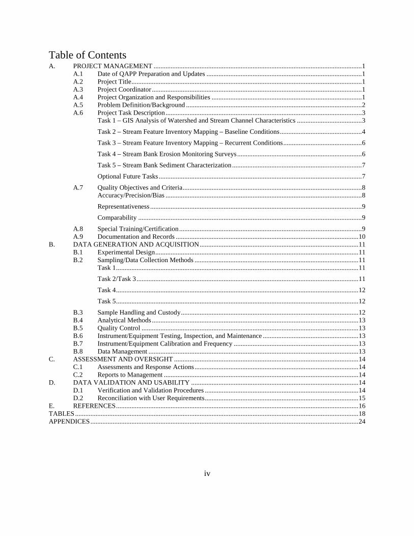
iv
Table of Contents A. PROJECT MANAGEMENT .......................................................................................................................... 1
A.1 Date of QAPP Preparation and Updates ........................................................................................... 1 A.2 Project Title ....................................................................................................................................... 1 A.3 Project Coordinator ........................................................................................................................... 1 A.4 Project Organization and Responsibilities ........................................................................................ 1 A.5 Problem Definition/Background ....................................................................................................... 2 A.6 Project Task Description ................................................................................................................... 3
Task 1 – GIS Analysis of Watershed and Stream Channel Characteristics ...................................... 3 Task 2 – Stream Feature Inventory Mapping – Baseline Conditions ................................................ 4 Task 3 – Stream Feature Inventory Mapping – Recurrent Conditions .............................................. 6 Task 4 – Stream Bank Erosion Monitoring Surveys ......................................................................... 6 Task 5 – Stream Bank Sediment Characterization ............................................................................ 7 Optional Future Tasks ....................................................................................................................... 7
A.7 Quality Objectives and Criteria ......................................................................................................... 8 Accuracy/Precision/Bias ................................................................................................................... 8 Representativeness ............................................................................................................................ 9 Comparability ................................................................................................................................... 9
A.8 Special Training/Certification ........................................................................................................... 9 A.9 Documentation and Records ........................................................................................................... 10
B. DATA GENERATION AND ACQUISITION ............................................................................................. 11 B.1 Experimental Design ....................................................................................................................... 11 B.2 Sampling/Data Collection Methods ................................................................................................ 11
Task 1 .............................................................................................................................................. 11 Task 2/Task 3 .................................................................................................................................. 11 Task 4 .............................................................................................................................................. 12 Task 5 .............................................................................................................................................. 12
B.3 Sample Handling and Custody ........................................................................................................ 12 B.4 Analytical Methods ......................................................................................................................... 13 B.5 Quality Control ............................................................................................................................... 13 B.6 Instrument/Equipment Testing, Inspection, and Maintenance ........................................................ 13 B.7 Instrument/Equipment Calibration and Frequency ......................................................................... 13 B.8 Data Management ........................................................................................................................... 13
C. ASSESSMENT AND OVERSIGHT ............................................................................................................ 14 C.1 Assessments and Response Actions ................................................................................................ 14 C.2 Reports to Management .................................................................................................................. 14
D. DATA VALIDATION AND USABILITY .................................................................................................. 14 D.1 Verification and Validation Procedures .......................................................................................... 14 D.2 Reconciliation with User Requirements .......................................................................................... 15
E. REFERENCES .............................................................................................................................................. 16 TABLES ...................................................................................................................................................................... 18 APPENDICES ............................................................................................................................................................. 24
1
A. PROJECT MANAGEMENT A.1 Date of QAPP Preparation and Updates Original QAPP: 01/30/17 by Wae Danyelle Davis; Revision 1: 07/21/17 by Wae Danyelle Davis as part of FAD regulatory review comment resolution. A.2 Project Title Quality Assurance Project Plan for Turbidity and Suspended Sediment Geomorphic Source Characterization in the Upper Esopus Creek Watershed, NY A.3 Project Coordinator Wae Danyelle Davis, Stream Studies Coordinator, Stream Management Program, NYCDEP, 71 Smith Avenue, Kingston, NY 12401, Telephone: (845) 340-7839, E-mail: [email protected] A.4 Project Organization and Responsibilities Table 1. Project Organization, Individuals and Responsibilities
Description
Name
Responsibility
Project Manager Wae Danyelle Davis
Oversee project, supervise data analysis and report generation
Field Team Leaders Wae Danyelle Davis
Emily Polinsky AWSMP Stream Assessment Coordinator Consultants
Data collection, data analysis, and report writing
Field Personnel WCC Interns
SCA Research Assistant AWSMP Field Staff Consultants
SFI, topographic surveys, sediment sampling, calibration and maintenance of equipment, data checking, data analysis, chain-of-custody
GPS Processing SCA Research Assistant
Emily Polinsky
Finalize GPS data corrections and processing
GIS Analyses Wae Danyelle Davis
Emily Polinsky SCA Research Assistant AWSMP Field Staff
Field sampling, calibration and maintenance of equipment, data checking, data analysis, chain-of-custody
Survey Data Entry SCA Research Assistant
WCC Interns AWSMP Field Staff
Enters field data into software
Data Review Wae Danyelle Davis Quarterly to annual data review for validation
and correction purposes Project QA Manager Dennis Dempsey
Contact regarding all QA/QC issues Report Coordinator Wae Danyelle Davis
Coordinates annual report
2
A.5 Problem Definition/Background The upper Esopus Creek is located in the Catskill Mountains of New York State and is part of New York City’s water supply system. In 1915 damming of a portion of the creek formed the Ashokan Reservoir splitting the creek into upper (upstream of the reservoir) and lower (downstream of the reservoir) segments. The Ashokan Reservoir watershed is 255 mi2 and is one of two reservoirs in the New York City Catskill Reservoir system and one of six reservoirs in the West-of-Hudson Catskill-Delaware system. The upper Esopus Creek watershed is approximately 192 mi2, and flows from the source, Winnisook Lake, to the Ashokan Reservoir near Boiceville, NY. Suspended-sediment concentration (SSC) and turbidity are primary water-quality concerns in New York City’s (NYC) water-supply system (U.S. Environmental Protection Agency, 2007). In the NYC water-supply system turbidity is largely caused by clay and silt rather than organic material (Effler et al., 1998; Peng et al., 2002; Peng et al., 2004). Sediment can originate from the watershed land surface and the active stream corridor (the stream bed and its adjacent banks and hillslopes) (Walling, 2005). In the upper Esopus Creek watershed, the main source of water to the Ashokan Reservoir, the active stream corridor is the assumed primary source of sediment and turbidity to the stream. Greater than 90% of the watershed terrain is forested and there are no substantive agricultural practices in the valley bottoms. A process-level understanding of sediment sources and transport pathways is required to develop effective strategies to reduce stream sediment and turbidity. In cases where the streambed or stream bank is the primary source of sediment, stream stabilization/restoration projects may be necessary to mitigate the problem. Without a process-level understanding of sediment and turbidity sources and transport pathways, sediment and turbidity reduction efforts will likely produce only short-term or limited benefits. DEP has used many years of geomorphic assessment and monitoring to identify chronic stream geomorphic reach-scale sources of suspended sediment loading that can lead to prolonged turbidity conditions in the upper Esopus Creek watershed. Turbidity reduction efforts in the Ashokan Reservoir through stream restoration practices are required as part of the NYC water supply FAD for the West-of-Hudson reservoir watersheds (U.S. Environmental Protection Agency, 2007). The 2013 revision to the FAD also required that DEP propose water quality monitoring studies designed to continue ongoing source characterization efforts and to evaluate the efficacy of stream restoration projects in reducing turbidity. The DEP proposal for the studies was submitted to the FAD regulators in November 2014 (DEP, 2014). The proposal called for a 10 year water quality monitoring, geomorphic monitoring and project implementation collaborative effort between DEP, USGS and AWSMP. In July 2016, DEP entered into the first of two 5-year contractual agreements with USGS to monitor and analyze suspended sediment concentration and turbidity as part of a nested set of studies coordinated by DEP’s Stream Management Program (SMP). This QAPP is an Appendix to the Study Design Report to be submitted to the FAD regulators as a FAD deliverable on January 31, 2017. The QAPP for the USGS water quality monitoring is provided in a separate document and is also an Appendix to the Study Design Report. The water quality monitoring studies are designed to (1) investigate the basin scale loading of suspended sediment/turbidity in the upper Esopus Creek watershed and “reach” scale loading of suspended sediment/turbidity in the Stony Clove Creek watershed; and (2) evaluate the effectiveness of specific stream management BMPs on reducing suspended sediment/turbidity at the reach to basin scale. For the purpose of this study, a stream “reach” refers to a segment of stream that is bracketed by upstream and downstream water quality monitoring stations. The monitored reaches are actually stream segments, typically greater than 0.5 miles that contain more than one uniform geomorphic stream reach. This was a necessary designation due to practical constraints on the number and feasible location of water quality monitoring stations. The term “basin” is synonymous with the monitored stream drainage area or watershed area. The monitored BMPs are stream restoration and hill slope stabilization practices that are designed to function as sediment and turbidity reduction projects (STRPs). Table 2 and Table 3 list the water quality monitoring stations for this study operated by USGS. Table 4 lists the current set of STRPs that will be monitored during this study.
3
DEP is responsible for ensuring completion of fluvial geomorphology and geology data collection and analysis to quantitatively and qualitatively inform the conditions that can influence suspended sediment/turbidity loading from the basin scale down to the stream geomorphic and monitoring reach scale. STRP implementation and morphometric monitoring is completed by the AWSMP through a separate contractual agreement with DEP. Geomorphic stream measurements provide an objective way of assessing stream physical characteristics and conditions influencing water quality. The prime objective of the project addressed by this QAPP is to quantitatively characterize the geomorphic and geologic sources of suspended sediment and turbidity monitored at USGS stream gage and water quality monitoring stations in the upper Esopus Creek watershed using GIS and field-based measurements. Specific focus is on the Stony Clove Creek watershed, the largest tributary to Esopus Creek. A.6 Project Task Description The project tasks necessary to accomplish the project objectives are primarily focused on the Stony Clove Creek watershed (SCW). Some tasks, or related existing data, are applicable to the upper Esopus Creek watershed (ECW) monitoring as well. Project tasks with their associated deliverables are presented in Table 4. Tasks 1 and 2 are applicable to both SCW and ECW. Tasks 3, 4 and 5 are applicable to SCW only. All project tasks use systematic processes (GIS measurements, GPS-mapping, stream channel measurements, and sediment sampling/sieving). Using consistent techniques will provide sound and factual information which can be easily replicated over a period of years and through changes in personnel. Task 1 – GIS Analysis of Watershed and Stream Channel Characteristics The objective for this task is to obtain watershed characteristics for monitored basins and stream reaches utilizing existing remote-sensed data. GIS is used to analyze the watershed and stream channel corridor conditions for monitored streams. Much of this task has been completed for most of the monitored streams as part of the stream management planning process, AWSMP stream assessment activities and Stony Clove watershed stream assessments completed by Milone & MacBroom, Inc. in 2015. Table 6 lists the streams in the upper Esopus Creek watershed that have been fully or partially assessed by these previous efforts. Arc ESRI 10.2 or greater will be used to
(1) Delineate and measure the watershed area for each water quality monitoring station. (2) Identify and delineate stream geomorphic management reaches (or units as referenced in stream
management plans) using a modified version of the Vermont Stream Geomorphic Assessment Protocols (VSGAP) (VT-ANR, 2004). The location of bridges and transportation infrastructure are added to the physical stream and valley characteristics used in the VT protocols. As noted in Section A.5 stream geomorphic management reaches do not coincide with the longer water quality monitoring reaches.
(3) For SCW, Complete a historic channel alignment analysis using available orthorectified aerial photography and standard methods (VT-ANR, 2004) to identify management and water quality monitoring reaches with historic channel migration. The current most recent aerial photography in the DEP GIS database is 1 ft resolution aerial imagery taken in April, 2009. Report the analysis as a % of monitored stream reach with active lateral adjustment per unit time.
(4) For SCW, review historic, recent and, if available, future aerial photography to identify areas of past, persistent and most recent stream erosion. Report the analysis as a list of erosion sites for qualitative assessment of channel stability.
(5) For SCW, measure the length of stream that is in contact with high terrace slopes, valley walls and other potential topographic features potentially susceptible to mass failure triggered by hydraulic erosion. Report the measured value as a % of the total length of monitored stream reach.
(6) For SCW, compute stream channel slope using a minimum of a 1 meter resolution digital elevation model (DEM) derived from the 2009 LiDAR data for the West-of-Hudson NYC water supply
4
watersheds. Length of stream for slope computation will be no greater than 100 meters and no less than 10 meters. Average slopes will be computed for management and water quality monitoring reaches. Slope will be used to compute total stream power (product of slope and discharge) and specific stream power (product of slope and discharge divided by channel width). Discharge will be determined using regionalized regression equations.
Additional optional GIS-based sub-tasks for SCW assessment may include:
If 1 meter DEMs derived from post-2009 LiDAR data are available and are of equal quality to the 2009 DEM in the DEP GIS library, identify areas of geomorphic adjustment using spatial cut-and-fill techniques available in Arc ESRI. As future aerial photography, equivalent to or greater than the quality of the 2009 aerial photography becomes available, add the new data to the historic channel alignment analysis. Compute other fluvial geomorphologic parameters that can include channel confinement and channel curvature. If these parameters are added to the list of study variables the QAPP will be revised to include methods and quality control measures.
Task 2 – Stream Feature Inventory Mapping – Baseline Conditions The objectives for this task include: mapping stream erosion suspended sediment sources; mapping existing and potential future STRPs. The primary field-based stream assessment activity for each monitored stream in this study consists of walking the stream with a handheld Global Positioning System (GPS) instrument to record a stream feature inventory (SFI) using a standardized GPS data dictionary developed by DEP (Attachment A). A SFI is a spatial catalog of information stored in a geodatabase that can be displayed, queried and spatially analyzed in a GIS platform. SFI’s are used as the foundation for diagnostic assessment in stream management planning for the Ashokan Reservoir watershed. Key stream features that are recorded typically include:
• Eroding banks • Fine sediment sources • Berm • Revetment • Bridges and culverts • Invasive species • Large woody debris jams • Impaired riparian vegetation • Headcuts • Bedrock grade control
From the data collected, useful statistics can be generated to quantify how much erosion is occurring, how much revetment is present, how much the stream comes into contact with clay, and how much of the floodplains are disconnected by berms within each stream management unit. Table 6 lists the monitored streams that have been or will be completed SFI’s for use in this study. The current set of SFI’s date from 2001 – 2015. All SFI’s completed since 2005 have used a version of the GPS data dictionary consistent with the version included in Attachment A. There were revisions to the data dictionary between 2005 and 2008 but these did not affect the attributes of the features detailed below that will be used in this study. Broadstreet Hollow is the only stream that currently has an SFI using the pre-2005 version of the data dictionary. That version did include sufficient feature attributes to track suspended sediment sources. For the purpose of this study the existing and planned SFI’s will be used for mapping the presence of the following geomorphic and geologic conditions that can influence suspended sediment loading:
5
Eroding Banks (Bank_P) – This feature is used to collect information on all eroding banks which are assumed to be the principal source of suspended sediment recruitment. See Attachment A for all attributes that are recorded in the field. Eroding banks can be defined by a sequence of upstream and downstream points with as many additional points in between as needed to capture changes to various attributes such as bank height, bank material or failure mechanism among several other attributes. The key attributes that may be used in this study are
• the combination of bank height and length (i.e. area of actively eroding bank), • failure mechanism (hydraulic, surficial, mass failure or a combination), • bank geology (identifies the primary geologic unit exposed in the bank, such as glacial till or alluvium) • bank material (identifies the dominant sediment material in the bank, such as gravel, cobbles, clay)
Potential metrics for monitored basins and/or reaches derived from this feature include: % active bank hydraulic erosion; % active bank mass failure; % erosional contact with alluvial sediment source; % erosional contact with non-alluvial sediment source. Headcuts (SFeat_P) – This feature is used for multiple purposes in defining stream bed morphology, channel alignment, channel type and the presence of headcuts. Headcuts are the locations in the stream longitudinal profile where significant drops in channel bed elevation appear to be migrating upstream and are indicative of reach scale streambed incision/degradation. Headcuts can incise into underlying glacial deposits that can be a significant source of suspended sediment/turbidity. The lowered streambed elevation can also destabilize adjacent streambanks that can trigger bank erosion through mass failure. Headcuts are recorded as a single point and include the elevation change between the top and bottom of the feature. The potential metric for monitored basins and/or reaches derived from this feature is simply whether headcuts are present in the monitored reach. Fine Sediment Sources (FineSedP) – This feature is supplemental to the eroding banks feature and is collected when fine sediment (clay and/or silt) exposures are observed in the stream bed, bank, hill slope or other sources such as when turbidity is observed in culverted discharge. See Attachment A for all attributes that are recorded in the field. The feature is defined as a single point or set of points delineating the observed source. The key attributes that may be used in this study are
• source geology (identifies primary geologic unit(s) as fine sediment source) • source location (identifies if source is in streambed, bank, both or other sources) • source volume (computed from recorded length, width and height of exposed sediment source)
Potential metrics for monitored basins and/or reaches derived from this feature include: % erosional contact with non-alluvial fine sediment source in bed; % erosional contact with non-alluvial fine sediment source in bank; % erosional contact with non-alluvial fine sediment source in both bank and bed. Revetment (Revet_P) – This feature is used to collect information on streambank stabilization through revetment protection (e.g. rip-rap, stacked rock walls, sheet piling, gabion baskets) and is an indicator of past active erosion mitigated through stabilization treatment. See Attachment A for all attributes that are recorded in the field. The feature is defined as a set of points delineating the extent, type and condition of the revetment. The key attributes that may be used in this study are
• type of revetment (identifies stabilization method; the use of sheet piling is often required when the eroding bank exposes easily erodible glacial lake sediment)
• length of revetment A potential metric for monitored basins and/or reaches derived from this feature is % revetment. Project Site (Project_P) – This feature is used to record the upstream and downstream location and extents of potential future or existing stream stabilization/restoration projects. The focus for this study will be on STRPs. See Attachment A for all attributes that are recorded in the field. The potential metric for monitored basins and/or reaches derived from this feature is % stream treated with STRP methods.
6
Task 3 – Stream Feature Inventory Mapping – Recurrent Conditions Objectives for this task include mapping/monitoring transient conditions of stream erosion suspended sediment sources; mapping/monitoring transient conditions of existing and potential future STRPs. SFI mapping will be repeated for each monitored stream in the Stony Clove watershed to track changes in geomorphic and geologic conditions that can influence suspended sediment loading and turbidity. The recurrent conditions mapping will be limited to the 5 SFI features described in Task 2. The current plan is to repeat SFI mapping for Stony Clove Creek, Warner Creek, Ox Clove Creek, Hollow Tree Brook and Myrtle Brook in 2019-2020 and again in 2024-2025. Optional SFI mapping may be implemented following potentially geomorphically significant flood events. An assumed minimum discharge threshold for assessing the need for optional SFI mapping is a 10-year flood as recorded at the Stony Clove long-term stream gage in Chichester. According to flood frequency analysis using annual peak flows from 1996 – 2015, the 10-year flood discharge is 12,257 cfs. Optional SFI mapping is contingent upon timing of the flood and availability of resources to implement the mapping. Potential metrics for monitored reaches are the same as for Task 2 with the addition of quantifying change in baseline conditions: % increase in exposed suspended sediment sources; estimated volume of material loss due to streambank erosion. Task 4 – Stream Bank Erosion Monitoring Surveys Objectives for this task include: monitoring stream bank erosion at a limited set of suspended sediment loading sites; monitoring stream bank erosion at potential future STRP sites for project selection prioritization. This task is specific to the Stony Clove watershed portion of the study. Using previous SFI mapping, select up to 10 stream bank erosion monitoring study (BEMS) sites that have the potential for contributing suspended sediment in the Stony Clove watershed and establish monumented topographic surveys for baseline conditions and recurrent monitoring. The number of monitored sites will depend in part on landowner access agreement. Recurring topographic surveys will be used to determine time-averaged bank erosion rates at the selected sites. Sites will be surveyed with upstream and downstream limits extending at least 2-5 bankfull widths above the eroding streambank. Survey methods will be either through use of total station technology or use of laser level technology. Total station technology allows for three-dimensional topographic mapping and laser level provides data for two-dimensional topographic profiling (e.g. cross-sections and longitudinal profiles). Sites will be established using total station technology to generate digital elevation models for each site. Subsequent surveys will be either technology. As of January 2017, four BEMS sites have been established with baseline conditions surveyed in November 2016: three in Warner Creek and one in Ox Clove. An additional site has been selected for Ox Clove and one possible site for Hollow Tree Brook, which will bring the total to five or six. Three to Four additional sites on Stony Clove Creek will be selected either from a set of sixteen monumented BEMS sites established in 2001 and resurveyed in 2012 (Coryat, 2014), or based on observed other bank erosion sites with potential for suspended sediment loading. Baseline conditions for all sites will attempt to be established in 2016-2017. Recurring surveys will occur at least every two years through the course of the study, with the next round of surveys scheduled for 2018-2019. Optional post-flood surveys will be completed contingent upon observed changes at the monumented bank erosion sites and availability of resources. Minimally, hydrologic conditions between biennial surveys will be factored into interpretation of measured erosion rates. Since this is not a systematic sampling of bank erosion rates with representative sites for all monitored reaches this data will not be used as a potential explanatory metric for monitored SSC and turbidity (this is approximated through the repeat SFI mapping in Task 3). It will be used to monitor potential treatment sites and improve understanding of streambank erosion process and the geologic and geomorphic conditions that can influence erosion and sediment entrainment.
7
Task 5 – Stream Bank Sediment Characterization Objectives for this task include: characterizing and categorizing distinct sedimentologic units exposed in streambanks; collection and grain size analysis of bulk samples representing sedimentologic units exposed in monitored eroding stream banks. This task is specific to the Stony Clove watershed portion of the study. A substantial amount of work has already been completed for this Task using past and recent geomorphic and geologic investigations and previous SFI results. Planned investigations in 2017-2018 will further characterize and categorize the observed geologic material potentially entrained into stream flow through stream bank erosion and mass wasting processes. Geologic material will be categorized into identifiable sedimentologic units. Representative bulk samples have been and will be collected and analyzed for grain size distribution as a means to account for the potential suspended sediment material that can be entrained by stream flow. If past sediment samples do not meet the specifications detailed in this QAPP the results will not be used, though they may be referenced for supporting quantitative information in describing sedimentologic unit sediment size distribution. Sedimentologic units will be ranked by percent composition of potential suspended sediment and mapped along the stream channel corridor using results of Tasks 2 and 3 and other available geologic investigations. For this study a sedimentologic unit is defined as a mappable geologic source of sediment that is identifiable in the field and has distinct sediment size distribution characteristics and erodibility characteristics. To date, DEP has categorized 5 distinct sedimentologic units exposed in eroding stream banks and mass wasting hill slopes:
• Holocene alluvium – stream sorted unconsolidated alluvium composed principally of sand to small boulder size material with some interstitial finer grained sediment. It is deposited by the stream occupying the valley during a previous lateral and vertical position for the stream channel. This is the typical and most abundant material exposed in the active valley bottom.
• Pro-glacial/Post-glacial alluvium – pro-glacial stream sorted unconsolidated alluvium with a similar sediment size composition but with the potential for more fine-grained sediment. It was deposited during the Pleistocene glaciation of the Catskills and/or early post-deglaciation stream sorting of glacially-derived sediment. This is typically exposed in mass failures in high glacial terraces
• Glacial Diamict or Till – unsorted and typically over-consolidated aggregation of sediment ranging in size from clay to boulders. It was deposited sub-glacially as lodgement till or in supra-glacial as moraines. This is typically exposed in stream contacts with valley wall slopes or glacial terrace hill slopes. It can also be exposed in streambed headcuts and channels that have incised below the stream alluvium. Previous investigations have identified more than one distinct glacial diamict in the Stony Clove watershed.
• Glaciolacustrine sediment (glacial lake deposits) – stratified and consolidated layers of clay, silt and some sand deposited subaqueously in impounded glacial meltwater. It is commonly exposed along the toe of eroding streambanks, as distinct layers in mass failing valley wall slopes and glacial terrace hill slopes. It can also be exposed in stream bed headcuts and channels that have incised below the stream alluvium.
• Colluvium – unsorted and variably consolidated aggregation of sediment ranging in size from clay to bouders. It is deposited from terrestrial erosional processes such as mass wasting following deglaciation or triggered by stream bank erosion. It is often a mix of two or more of the other sedimentologic units and can be very variable in sediment composition.
Further investigation may result in more sedimentologic unit categories. This data will be used for qualitative accounting of potential suspended sediment yield from topographically surveyed or SFI-mapped monitored eroding streambanks. Coarse estimates of the potential volume of each sedimentologic unit removed through monitored bank erosion will be compared with the relative difference in magnitude of monitored SSC and turbidity. Optional Future Tasks No further suspended sediment source characterization tasks are planned at this time. Consideration has been given to characterizing longitudinal changes in stream bed material size distribution and suspended sediment source fingerprinting. If additional resources are available these two tasks will be reconsidered for inclusion in this study.
8
A summary of all study variables used to derive metrics for analysis is presented in Table 7. A.7 Quality Objectives and Criteria Since a substantial portion of the geomorphic and geologic data used in this study has been obtained through previous efforts without use of a QAPP to guide data collection there will be two categories of data quality: pre-QAPP and post-QAPP. One of the data management activities in 2017 will be to review the pre-QAPP data and identify if there are any deficiencies in meeting the quality objective criteria described in this QAPP. If there are deficiencies, the Project Manager will evaluate whether the deficiencies require re-acquisition of data for use in this study. The data quality objectives for the geomorphic investigations to support suspended sediment source characterization are described below. Table 8 provides minimum standards for measurement tolerances for some of the project Tasks. Accuracy/Precision/Bias Task 1 All GIS source data is located in the DEP GIS library and has met high standards of quality assurance/control documented in associated metadata files for each GIS layer/feature used in this analysis. Measurements will be performed by individuals trained in GIS analytical techniques. Digitizing stream centerlines, channel boundaries and other features will be performed at a zoom-level that allows for accurate and precise placement of the digitized points and lines without loss of sufficient resolution to identify the analyzed features. All digitized features in the Stony Clove watershed study and measurements will be checked independently for accuracy, precision and user bias in selecting line or point location. Task 2 and 3 In this study, SFI data is used to compute lengths of bank erosion/hill slope mass failure, stream contact with fine sediment sources, revetment and STRPs. The lengths are reported as percentages of the total length of a monitored reach and/or basin or as percentages of the total measured erosional contact (Table 7). Given the high magnitude of the total length values (hundreds to thousands of feet) the tolerance for accuracy in the actual metrics used in the analysis allows for accuracy tolerance to be within several feet of an actual length. Care will be taken to keep the accuracy of all measurements to within 3 feet. Precision can be ensured by using the same analytical instruments throughout the whole data collection process. While there have been improvements in technology since the first SFI in the upper Esopus Creek watershed was completed in 2001, fortunately Trimble GPS technology has been used for all SFI’s completed to date and will be used for all future SFI data collection. Since 2005, Trimble rugged handheld computers with integrated high accuracy global navigation satellite system (GNSS) receivers have been used to acquire SFI data. Data collected from 2015 on has used Trimble Geo-XH 6000 series or Trimble 7X models enabled with H-Star technology delivering 10 cm (0.33 ft) real-time or post-processed accuracy. User bias is the most challenging data quality objective to control in the SFI tasks. All SFI’s were completed by DEP, Ulster and Greene County Soil and Water Conservation District personnel, or consultants. All field leaders were trained by a qualified fluvial geomorphologist (2000 – 2005: Sarah J. Miller; 2005 – 2015: Wae Danyelle Davis). User bias is primarily manifest as selecting different upstream/downstream extents of active erosion, collecting the data points at different distances from the eroding bank, and collecting an insufficient number of points per feature. Controls on user bias going forward in the study are similar to the controls used prior to 2017: (1) Each feature recorded by GPS should have an accompanying photo clearly showing the feature as the data is being collected; optionally pin or stick flags can be placed at the recorded feature for each photo. (2) Bank erosion points should be collected at the toe of the eroding bank as close as possible to the bankline. If this is not practicable, then the points should be collected at the top of the feature and the horizontal distance to the bank toe estimated using a laser range finder (TruPulse 360R model or equivalent). (3) All mapped features should have at least 10 GNSS points to compute the feature position. (4) Ensure that any individual responsible for data collection is properly trained by the Project Manager.
9
Additional potential impacts on accuracy that can affect the study include measurements of streambank height, bank angle, judgment calls on failure mechanisms and bank material geology. Appropriate training in measuring bank dimensions and identifying bank geology will be provided by the Project Manager as a means of ensuring accuracy associated with bank feature measurements and bank material interpretation. Task 4 Stream bank erosion monitoring is essentially stream morphology data collection. As with the SFI data acquisition precision can be ensured by using the same analytical instruments throughout the whole data collection process. The existing BEMS sites have been surveyed using total station technology and laser level technology. The assumed technology for future topographic surveys will be total station, allowing for three-dimensional surveys linked to an established coordinate system such as the state plane coordinate system or the Universal Transverse Mercator (UTM) coordinate system. Some repeat surveys may be limited to cross-sections and longitudinal profiles using laser level technology. Table 8 provides the acceptable accuracy limits for all topographic survey measurements. Available official geodetic survey benchmarks will be fully referenced when available. If geodetic survey benchmarks are not available study benchmarks will be installed, elevations established and referenced for each survey. Checking for errors and inconsistencies will be performed regularly in the field by each field team member, and acceptable note-taking and paper and electronic reporting formats will be adhered to. Precision can be further improved by insuring the survey instruments are properly calibrated according to the manufacturer’s specifications. If professional surveyors are hired to complete the surveys, they will need to provide documentation that the instruments are properly calibrated. Task 5 Accuracy, precision and quality control on bias in sediment sampling for grain-size distribution analysis will be ensured through collecting bulk samples from BEMS site stream banks in sufficient quantity to use the prescribed ASTM standard methods for particle-size analysis specified in Section B.4 Analytical Methods. These ASTM specifications will be a part of the order for laboratory analysis. If a laboratory cannot provide these standard methods, it will be not be used. Representativeness This data quality objective criteria does not necessarily apply to Tasks 1-3, since the tasks are comprehensive assessments of the entire study area streams. For Tasks 4 and 5, representativeness depends largely on randomized sampling covering a sufficient sample size. However, this current study scope is not intended to use bank erosion monitoring and sediment sampling to be representative of the monitored streams. The BEMS sites and associated sampling are primarily intended to help inform future STRP selection. The sediment sampling in Task 5 will be considered representative of the primary sedimentologic units that are currently assumed to contribute to suspended sediment load. At least two to three samples per sedimentologic unit present in BEMS sites will be analyzed to account for potential variability in sediment size distribution in the sedimentologic units. Comparability The QAPP will standardize the protocols for data measurement and collection. All field personnel collecting geomorphic data for this study will be trained in the standardized methodology, which will help ensure data collection is repeatable and comparable over time, personnel changes, or against data from similar projects. These data must be collected with the same tolerances and methods for each SFI mapping, fluvial geomorphologic survey and sampling within the project. When collection techniques remain consistent, these data become more valuable for use in comparison to future and past measurements. A.8 Special Training/Certification All work for this project will be conducted and/or overseen by DEP, AWSMP, WCC interns, SCA interns and
10
consultants trained in standard GIS analytical techniques, stream feature inventory mapping, fluvial geomorphic survey techniques and sediment sampling. The Project Manager and all identified Field Team Leaders have been trained in applied fluvial geomorphology assessment techniques taught by Wildland Hydrology, Inc. The Project Manager has a minimum of 16 years of fluvial geomorphology data collection, analysis, interpretation, and stream survey techniques experience. Some of the work for all Tasks, except Task 3, has been completed in previous investigations; however, all work was completed by qualified fluvial geomorphologists and/or individuals trained by qualified fluvial geomorphologists. The Project Manager is responsible for assuring that that all future data collection is by personnel trained to perform the data collection task. The Project Manager will conduct the training or ensure that qualified individuals conduct the training in GIS analysis and fieldwork. If consultants are used for data collection the Project Manager will ensure that the consultants are qualified. GIS training will incorporate techniques for digitizing channel centerlines and streambanks and using the VSGAP GIS analytical steps. Fieldwork training will incorporate operation and appropriate use of field instruments and equipment, procedures for taking accurate, comprehensive and readable survey notes, analyzing field data, and understanding the appropriate need for accuracy and quality control in data collection. All field assistants are required to be familiar with the QAPP. The training for interns also includes basic fluvial geomorphology theory, stream classification, and assessment techniques. A.9 Documentation and Records The QAPP will be maintained by the Project Manager in a project specific digital folder on a network drive located in Kingston, NY and accessible to all DEP project personnel. Updates to the QAPP and other Study Design documents will be distributed to all project personnel immediately and will be highlighted during project meetings. Version control will be reported in Section A.1 Date of QAPP Preparation and Updates. All study documents will also be stored electronically in the project folder on the network drive in Kingston, NY. All files on the network drive are backed up regularly by the DEP OIT staff. All fieldwork starting in 2016 will be recorded in project dedicated field notebooks and where appropriate on standardized field forms. Fieldwork documentation prior to 2016 will be reviewed by the Project Manager to verify that documentation is sufficient to meet the project quality objectives and documentation standards. Any necessary modifications to existing documentation will be annotated and described in an associated metadata file. All blanks for data/information entry are to be used. If there is no data/information for the specific task then a line is drawn through the blank to demonstrate that data was not unintentionally not recorded. Changes to recorded data will not be erased, but crossed out and the updated information will be written next to the original value. Changes should be dated and initialed by the person making the changes. Hard copies of field data, field notes, printed photos and maps will be stored in 3-ring binders and/or file folders in the DEP Kingston, NY office. Copies of all field-recorded observations and data will be scanned and stored electronically in the digital project folder on the network drive. All electronic field documentation, such as GPS points and electronic notes will be stored in a manner similar to the scanned fieldwork documentation. Photographs will be collected using a digital camera, and when possible GPS-enabled to be capable of collecting and storing the latitude/longitude point at which a photograph is collected. If the digital camera is not GPS-enabled and the photograph is taken during Tasks 2 and 3 SFI mapping, field notes and GPS digital notes will record the photograph ID generated by the camera. Photographs for Tasks 4 and 5 will be recorded in a standardized photograph log field form. All photographs will be stored electronically in the project folder on the network drive.
11
B. DATA GENERATION AND ACQUISITION B.1 Experimental Design The geomorphic and geologic data collected and analyzed for this project is intended to support the experimental design documented in the Study Design Report. The experimental study design is principally focused on the water quality monitoring described in the QAPP prepared by USGS. The geomorphic and geologic data will be used to help interpret the upper Esopus Creek watershed and Stony Clove watershed water quality monitoring results. The water quality monitoring uses two types of monitoring sites, (1) primary monitoring sites will be used for in situ turbidity monitoring and suspended sediment sampling to calculate SSLs and yields, 2) secondary monitoring sites will be used for in situ turbidity monitoring only. The monitoring stations for the upper Esopus Creek watershed are identified in Table 3. There are 3 primary monitoring stations on Esopus Creek, effectively dividing the stream into three monitored sections. There are 5 additional primary monitoring stations at the approximate downstream limits of the 5 largest tributary streams. An additional 2 secondary monitoring stations are located at the approximate downstream limits of 2 additional tributaries. Water quality monitoring for the upper Esopus Creek watershed is limited to the sub-basin scale. Tasks 1 and 2 will provide data and interpretation of spatially distributed geomorphic and geologic conditions that will be used to characterize sub-basin scale physical characteristics that may influence suspended sediment yield and/or turbidity at the monitoring station. The monitoring stations for the Stony Clove watershed study are identified in Table 2. There are 2 primary monitoring stations on the Stony Clove, one representing the sub-basin scale (also used in the upper Esopus Creek watershed study) and the other representing the upper watershed above the three main tributary streams that have known suspended sediment sources. There are 4 additional primary monitoring stations for each of the main tributaries. There are 14 secondary monitoring stations that serve to segregate the monitored streams into monitored segments: 8 on Stony Clove Creek, 4 on Warner Creek, and 1 each on Ox Clove Creek and Hollow Tree Brook. Myrtle Brook does not have a secondary monitoring station as it is the smallest of the four monitored tributaries and has no mapped high yielding suspended sediment sources. Tasks 1 – 3 will provide data and interpretation of spatially distributed geomorphic and geologic conditions that will be used to characterize sub-basin to stream segment scale physical characteristics that may influence suspended sediment yield and/or turbidity at the monitoring stations. Tasks 4 and 5 are primarily intended to help select potential future STRPs for inclusion in the study. Since there are a limited number of stream bank erosion monitoring sites that are not systematically distributed throughout the Stony Clove watershed and represented in each monitored stream segment they have negligible value in correlating monitored bank erosion and sediment entrainment to monitored turbidity and/or suspended sediment load. B.2 Sampling/Data Collection Methods Consistency in data collection is vital. Basic procedures conducted for GIS analysis, SFI mapping and fluvial geomorphology data collection are intended to be consistent from year to year and to yield precise, accurate and comparable assessments of stream channel geomorphologic conditions. Task 1 Standard GIS digital measurement techniques will be used for obtaining lengths and areas of select features as well as digitizing stream channel centerlines and stream bank lines. Task 2/Task 3 The SFI field team is headed by a qualified fluvial geomorphologist/geoscientist that has been trained by DEP personnel and other professionals in the use of the SFI data dictionary and methods. SFI data will be collected using Trimble Geo-XH 6000 series or Geo-7X (or better) units for each stream bank and the stream bed from the upstream extent of the study stream to the downstream extent. A minimum of 10 points need to be recorded per feature in
12
order to ensure sufficient accuracy and precision in the final averaged representative point. Field staff will collect the features specified for Tasks 2 and 3 with the GPS unit standing as close to the feature as possible. Photographs should be taken for each SFI recorded feature. Any physical measurements needed to record stream bank height, length, angle or dimensions of fine sediment sources should use an engineer’s survey tape with 0.1 ft increments and survey rod with 0.01 increments, or use a laser range finder with an accuracy equivalent to the Trupulse 360R. Task 4 Stream channel topographic survey methods and equipment will be consistent with the protocol provided in Harrelson et al 1994. All cross sections will be monumented with capped rebar (no less than 3 ft long) driven vertically into the ground at least 10 feet from the top of the monitored streambank, or greater if the potential for more than 10 feet of lateral bank retreat is present. All monuments will be surveyed by a Total Station to determine the horizontal coordinates and elevation. The monuments will also be recorded by GPS using Trimble Geo-XH 6000 series or Geo-7X (or better) units. The number of cross sections per monitoring site will be determined by stream bank erosion complexity. If a site is less than 100 feet, has relatively uniform height and material composition, a single monumented cross section may be adequate. More typically at least two to three cross sections may be required to represent site variability. Care will be taken on conducting the cross section survey so that the work itself does not cause bank erosion. All bank profiles will be sketched in the notes, with data points labeled and any comments on bank irregularities (undercut banks, root exposure, etc) indicated. Changes in bank material composition will be described and included in the bank profile. Cross sections will be analyzed over time to estimate that amount of channel and bank erosion within the selected study site. Longitudinal profiles will be used to assess whether the monitored site is aggrading or degrading. An alternative to just surveying cross-sections and longitudinal profiles is to survey the total topography of the eroding streambank, the associated channel and immediately adjacent terrain using total station technology. This allows for the full bank to be monitored and for cross-sections and longitudinal profiles to be excerpted from the processed digital elevation data. This is a much more labor intensive effort and will be evaluated for use in 2017. If this is the preferred method for future topographic surveys at bank erosion monitoring sites the Study Design Report and this QAPP will be revised accordingly. Task 5 All identified sedimentologic units will be sampled for grain size distribution analysis by qualified project personnel or by a qualified geotechnical laboratory. All sample locations will be recorded by GPS using Trimble Geo-XH 6000 series or Geo-7Z (or better) units. Attempts will be made to have each sedimentologic unit present in a BEMS site sampled and analyzed. Sediment sample collection will be bulk samples collected in sufficient volume to adequately represent the distribution of observed sediment sizes. Smaller samples are needed for silt/clay deposits and larger samples are needed for coarse alluvial deposits or glacial till with cobble size sediment clasts. B.3 Sample Handling and Custody GPS data will be collected for Tasks 2-5. All GPS files recorded in the field will be processed in the DEP office in Kingston, NY or in the AWSMP office in Shokan, NY, unless collected and processed by consultants. All GPS processing will be by the appropriate personnel identified in Table 1. All GPS data collected in the field should be reported on field forms or in field books which will be scanned and stored in files as metadata for the GPS data. Photo numbers for sampling and monitoring will be reported on field forms or in field books. Starting in 2017, when appropriate, e.g. sampling or monitoring sites, a small white board and dry erase marker will be used at a photo site to identify location, date, time and any appropriate notes. All survey data will be recorded on field forms and/or electronically if using a total station. The Field Team Leaders will be responsible for collecting all field forms if used and ensuring that all forms are completed. The Field Team Leaders will ensure that all field forms are scanned and stored digitally in project folders, photo-copied and stored in 3-ring binders. The Project Manager will check that this has been completed on a weekly basis. If a total station is
13
used, all digital files will be accompanied with a meta-data file explaining the provenance, date, and intended use of the survey data Starting in 2017, sediment samples that will be sent to a geotechnical laboratory for analysis will be labeled with the date, location, sample site, sample name, and analytical method. Photographs of all samples will be taken and digitally stored with the analytical results. Some coarse-grained alluvium samples may be sieved in the field and will be similarly documented. B.4 Analytical Methods All spatial analysis will be performed with ArcGIS 10.x software. All stream morphology data will be entered into and analyzed in the RiverMorph software package and/or MS Excel files. All sediment sample results will be stored and analyzed in MS Excel files. All statistical correlation analyses will be performed using either Excel, MiniTab or an equivalent statistical analysis software package. The testing methods for particle-size analysis that will be used will be equivalent to the ASTM D-422 (gradation), ASTM D-1140 (wet wash) and ASTM D-854 (specific gravity/hydrometer) for sediment smaller than 0.075 mm (fine sand). B.5 Quality Control This QAPP includes the prescribed means to ensure quality control in field and analytical procedures for data collected starting in 2017. In addition to the steps described elsewhere in the QAPP:
• The Field Team Leader will ensure that there are enough blank field forms for the day’s work. • All data field forms will have quality control information on the bottom: spaces to initial and date four
steps in the quality control process (data validation, data verification, data entered and data checked). See Section DATA VALIDATION AND USABILITY for details.
• The Project Manager reviews all field forms no less frequently than on a weekly basis for accuracy and thoroughness. Illegible hand writing is neatened and details added to notes, if needed.
B.6 Instrument/Equipment Testing, Inspection, and Maintenance Trimble ruggedized hand-held computers and all topographic survey instruments used by project personnel are tested, inspected and maintained by DEP and AWSMP personnel using methods specified in instrument user manuals. All laser levels used in topographic surveying are tested prior to use in each field season. Copies of documentation of equipment maintenance and verification checks will be stored with the project-dedicated digital directory of folders on the network drive in Kingston, NY. B.7 Instrument/Equipment Calibration and Frequency Laser levels are checked seasonally for accuracy and precision through use of standard peg test methods. If a laser level cannot be calibrated by project personnel is will be sent to a qualified technician for calibration. Copies of documentation of laser level peg tests and calibration will be stored with the project-dedicated digital directory of folders on the network drive in Kingston, NY. B.8 Data Management Field crews are encouraged to use pencils with 2H or HB lead to document all field data and information. All error corrections are completed by placing a single horizontal line through the error, recording the new data next to or above the erroneous record(s) and initialing the correction. All data will be entered into the appropriate software identified in section B.4 Analytical Methods and stored in the project dedicated directory of folders on the network drive located in Kingston, NY.
14
C. ASSESSMENT AND OVERSIGHT C.1 Assessments and Response Actions Attention to quality is a primary consideration for this project. The Project Manager is responsible for oversight of all project activities and will formally review the performance of the field crew at various times during the field work to ensure proper data collection. If the Project Manager is also collecting data, then the Project QA Manager will perform this task. The Project QA Manager will ensure that all QA procedures outlined in this QAPP are followed. C.2 Reports to Management The Field Team Leaders will report on the status of the field work to the Project Manager on a weekly basis and report on any issues that might compromise the quality of the project as they arise. The Project Manager will report project status to the Stream Management Program Unit Chief, Elizabeth Reichheld on a monthly basis. The Project Manager is also the Project Coordinator with the USGS-directed component of the Esopus Creek watershed turbidity and suspended sediment monitoring study. Quarterly to semi-annual meetings will be convened to coordinate the two primary efforts in this collaborative project.
D. DATA VALIDATION AND USABILITY D.1 Verification and Validation Procedures All field data collected since 2017 used in the Study will be verified and validated. Data collected prior to this will be reviewed to assess validity and usability for the Study. Future field data collection and data entry activities are subject to verification and validation reviews by the Field Team Leaders, Project Manager or by a designated alternate, such as a qualified consultant. Task 2/Task 3 The SFI field team will record data in the Trimble Geo units and in accompanying field notes using a standardized field form (see Attachment B for sample of an SFI field form that may be adapted for this study) and field maps of the assessed stream. The Project Manager will review field forms for completeness and legibility. The Project Manager will also ensure that the recorded GPS features used a minimum of 10 position points to derive the feature position. If geological or geotechnical choices are required (e.g. interpreting source geology in an eroding bank feature), photos and observational notes will be reviewed by a qualified geologist, if not collected by one. If needed, second opinions may be required. Task 4 There are two basic approaches to obtaining survey data for Task 4. The first (and currently preferred) approach is to procure the services of licensed surveyors to complete topographic surveys using total station technology with all data stored digitally in the field. The licensed surveyors will be required to process all data and provide documentation of geodetic benchmarks and other survey controls used to complete the survey. The second approach is for DEP and/or AWSMP personnel to complete cross-section and longitudinal profile surveys using laser level technology. This requires the recording of data on field forms and optionally in digital format using a ruggedized laptop or tablet. Sample field forms that may be adapted for this field study are included in Attachment B. Validation reviews of laser level field data are conducted at the end of each survey day, where the Field Team Leader or the Project Manager reviews field forms for completeness and screens the data for potential errors. If the forms are not complete, all blank items are filled if needed, or a line is drawn through them if there is no data/information needed. If errors are found, they are corrected before computer data entry begins. If consistent errors are found or blanks continually not filled, retraining on the particular issue occurs before the next field day. The Field Team Leader or the Project Manager validates the data collected for that particular day by signing the bottom of the field forms in the validation space at the conclusion of each field day.
15
Verification reviews for field-based activities are conducted by the Field Team Leader, Program Manager or the QA Manager to ensure data are collected in accordance with this QAPP. This is achieved through use of a verification checklist created by the Project Manager, which will include proper documentation of data collected during laser level surveys and appropriate reconciliation of documentation errors made during field activities (see Attachment B for sample checklists). The verification review is conducted at the end of the field day, or the field week. Requisite corrective actions are identified and imposed prior to subsequent survey data acquisition. Task 5 Verification and validation procedures for sediment sampling for grain-size distribution analysis will include reviewing field documentation to ensure there is clear identification of sample location, sedimentologic unit sampled, sample volume noted and sufficient for analysis, and that specific ASTM standards for sample analysis are requested. Any decisions regarding the usability of data will ultimately be left to the Project Manager in consultation with the QA Manager. It should be noted that the highest value data in the sediment source characterization component of the Study is the Task 2 and Task 3 data, which will be used to derive potential metrics for explaining observed and/or predicting reach-scale suspended sediment loading. Task 4 and 5 data will also be required to meet the aforementioned verification and validation standards, though the data is used solely for (1) helping prioritize potential future treatment sites and (2) helping improve understanding of streambank erosion process contributions to suspended sediment loading from assumed high loading source sites. When it is found that data do not meet the quality objectives detailed in this QAPP or do not adhere to the quality control measures, the Project Manager may determine what corrective action must be taken. Incomplete data may lead to the need for re-survey or re-collection of SFI features. D.2 Reconciliation with User Requirements In situations where the GPS equipment or survey equipment has been shown to be faulty, the equipment will be repaired/replaced. If it is shown that better training is required to ensure data quality will meet the use requirements the Project Manager may request additional support. The focus of the data interpretation this QAPP serves is to (1) identify and characterize channel suspended sediment sources for the monitored Upper Esopus Creek sub-basins, (2) identify and characterize channel suspended sediment sources at the “reach” scale for the Stony Clove Creek watershed; and (3) characterize temporal changes in Stony Clove Creek watershed suspended sediment sources in response to hydrologic events, geomorphic recovery following hydrologic events, and source treatment through STRPs or other management actions. This interpretation is based on the Task 2 and 3 SFI work. Limitations in the SFI data, survey data and sediment sampling data will be clearly identified in the analysis of the physical characterization data with the USGS water quality monitoring data. One such potential limitation is with the SFI data. Spatial data collected prior to 2015 did not have the higher potential accuracy (0.33 ft) available with the Trimble Geo-XH 6000 or Trimble 7X models enabled with H-Star technology. While the pre-2015 data doesn’t match the potential level of accuracy of the newer technology, the data does meet the accuracy objective of 3.0 ft stated in Section A.7. This is considered an acceptable limitation for the baseline data for the sub-basin, since the data will be used to characterize cumulative lengths of eroding streambanks that total in thousands of feet on the sub-basin scale. The study design does not anticipate repeat SFI surveys except for the Stony Clove sub-basin. If repeat SFI surveys occur in the other monitored sub-basins the SFI data for those sub-basins will be updated in the analysis. The 2013 SFI for Stony Clove Creek and the 2010 SFI for Warner Creek provides the baseline source characterization data for the Stony Clove Creek watershed reach-scale monitoring and meet the 3.0 ft accuracy objective. Warner Creek has repeat SFI’s for 2011-2012 and 2015 for the lower 3.2 km of stream length. Repeat surveys conducted as part of the study design will occur beginning in 2018 and will use the higher resolution technology. Differences in potential spatial resolution between time series data will be identified and assessed for
16
potential impact on metrics derived as potential explanatory variables described in Section A.6. Potential limitations with the topographic survey data obtained in Task 4 are related to potential errors that should be addressed in the data validation and verification process or future changes in survey technology that may improve spatial resolution in repeat surveys. Potential limitations with the sediment sampling data obtained in Task 5 are limited to adequacy of sample size and representativeness of the possible sedimentologic units. Neither of these Tasks affect the primary objectives of the study to characterize the spatial distribution of suspended sediment sources and the evaluation of STRP effectiveness in reducing turbidity and suspended sediment through water quality monitoring. These and other potential limitations associated with these tasks will be discussed and evaluated through the course of the study. Quarterly to semi-annual project collaboration/coordination meetings between DEP and USGS Principal Investigators will be used to review data collection and analysis results for both efforts. This section of the QAPP will be revised as needed to account for any changes that may remove or add potential limitations.
E. REFERENCES Harrelson, C.C., C.L. Rawlins, and J.P. Potyondy. April 1994. Stream channel reference sites: an illustrated guide to field technique. United States Department of Agriculture, Forest Service General Technical Report RM-245. Rocky Mountain Forest and Range Experiment Station, Fort Collins, CO. Church, Michael, 2002, Geomorphic thresholds in riverine landscapes: Freshwater Biology, v. 47, no. 4, p. 541–557. Coryat, M. 2014. Analysis of the Bank Assessment for Non-point Source Consequences of Sediment (BANCS) Approach for the Prediction of Streambank Stability and Erosion along Stony Clove Creek in the Catskills. Syracuse University. Theses – ALL Effler, S.W., Perkins, M.G., Ohrazda, Nicholas, Brooks, C.M., Wagner, B.A., Johnson, D.L., Peng, Feng, and Bennett, A., 1998, Turbidity and particle signatures imparted by runoff events in Ashokan Reservoir, NY: Lake and Reservoir Management, v. 14, no. 2–3, p. 254–265. McHale, M. R., and J. Siemion, 2014, Turbidity and suspended sediment in the upper Esopus Creek watershed, Ulster County, New York, US Geological Survey Scientific Investigations Report 2014-5200, 42 p., http://dx.doi.org/10.3133/sir20145200. DEP, 2014, Ashokan Stream Management Program Water Quality Studies Proposal, (Prepared in accordance with Section 4.6 of the NYSDOH revised 2007 Filtration Avoidance Determination), 11 p. Peng, Feng, Johnson, D.L., and Effler, S.W., 2002, Suspensoids in New York City’s drinking water reservoirs—Turbidity apportionment: Journal of the American Water Resources Association, v. 38, no. 5, p. 1453–1465. Peng, Feng, Johnson, D.L., and Effler, S.W., 2004, Characterization of inorganic particles in selected reservoirs and tributaries of the New York City water supply: Journal of the American Water Resources Association, v. 40, no. 3, p. 663–676. Rosgen, D.L., 1997, A geomorphological approach to restoration of incised rivers, in Wang, S.S.Y., Langendoen, E.J., and Shields, F.D., Jr., eds., Proceedings of the conference on management of landscapes disturbed by channel incision: Oxford, Miss., The University of Mississippi, p. 12–22. Siemion, J., M. R. McHale, and W. D. Davis (2016), Suspended-sediment and turbidity responses to sediment and turbidity reduction projects in the Beaver Kill, Stony Clove Creek, and Warner Creek, Watersheds, New York,
17
2010–14, U.S. Geological Survey Scientific Investigations Report 2016-5157, 28 p., https://doi.org/10.3133/sir20165157. U.S. Environmental Protection Agency, 2007, New York City filtration avoidance determination: U.S. Environmental Protection Agency Web page, accessed July 15, 2013, at http://www.epa.gov/region2/water/nycshed/2007fad.htm. VT-ANR, 2004. Vermont Agency of Natural Resources Stream Geomorphic Assessment Protocols Handbook: Remote Sensing and Field Surveys Techniques for Conducting Watershed and Reach Level Assessments. Walling, D.E., 2005, Tracing suspended sediment sources in catchments and river systems: Science of the Total Environment, v. 344, no. 1–3, p. 159–18
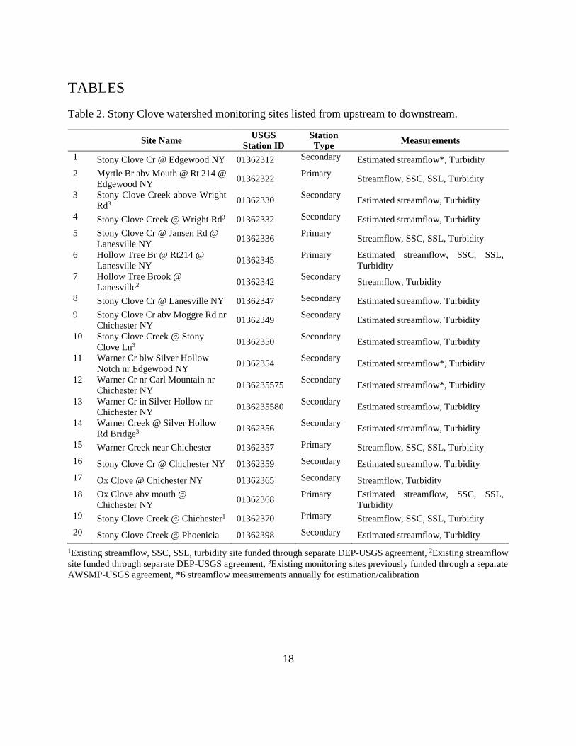
18
TABLES Table 2. Stony Clove watershed monitoring sites listed from upstream to downstream.
Site Name USGS Station ID
Station Type Measurements
1 Stony Clove Cr @ Edgewood NY 01362312 Secondary Estimated streamflow*, Turbidity 2 Myrtle Br abv Mouth @ Rt 214 @
Edgewood NY 01362322 Primary Streamflow, SSC, SSL, Turbidity
3 Stony Clove Creek above Wright Rd3 01362330 Secondary Estimated streamflow, Turbidity
4 Stony Clove Creek @ Wright Rd3 01362332 Secondary Estimated streamflow, Turbidity 5 Stony Clove Cr @ Jansen Rd @
Lanesville NY 01362336 Primary Streamflow, SSC, SSL, Turbidity
6 Hollow Tree Br @ Rt214 @ Lanesville NY 01362345 Primary Estimated streamflow, SSC, SSL,
Turbidity 7 Hollow Tree Brook @
Lanesville2 01362342 Secondary Streamflow, Turbidity
8 Stony Clove Cr @ Lanesville NY 01362347 Secondary Estimated streamflow, Turbidity 9 Stony Clove Cr abv Moggre Rd nr
Chichester NY 01362349 Secondary Estimated streamflow, Turbidity
10 Stony Clove Creek @ Stony Clove Ln3 01362350 Secondary Estimated streamflow, Turbidity
11 Warner Cr blw Silver Hollow Notch nr Edgewood NY 01362354 Secondary Estimated streamflow*, Turbidity
12 Warner Cr nr Carl Mountain nr Chichester NY 0136235575 Secondary Estimated streamflow*, Turbidity
13 Warner Cr in Silver Hollow nr Chichester NY 0136235580 Secondary Estimated streamflow, Turbidity
14 Warner Creek @ Silver Hollow Rd Bridge3 01362356 Secondary Estimated streamflow, Turbidity
15 Warner Creek near Chichester 01362357 Primary Streamflow, SSC, SSL, Turbidity 16 Stony Clove Cr @ Chichester NY 01362359 Secondary Estimated streamflow, Turbidity 17 Ox Clove @ Chichester NY 01362365 Secondary Streamflow, Turbidity 18 Ox Clove abv mouth @
Chichester NY 01362368 Primary Estimated streamflow, SSC, SSL, Turbidity
19 Stony Clove Creek @ Chichester1 01362370 Primary Streamflow, SSC, SSL, Turbidity 20 Stony Clove Creek @ Phoenicia 01362398 Secondary Estimated streamflow, Turbidity
1Existing streamflow, SSC, SSL, turbidity site funded through separate DEP-USGS agreement, 2Existing streamflow site funded through separate DEP-USGS agreement, 3Existing monitoring sites previously funded through a separate AWSMP-USGS agreement, *6 streamflow measurements annually for estimation/calibration
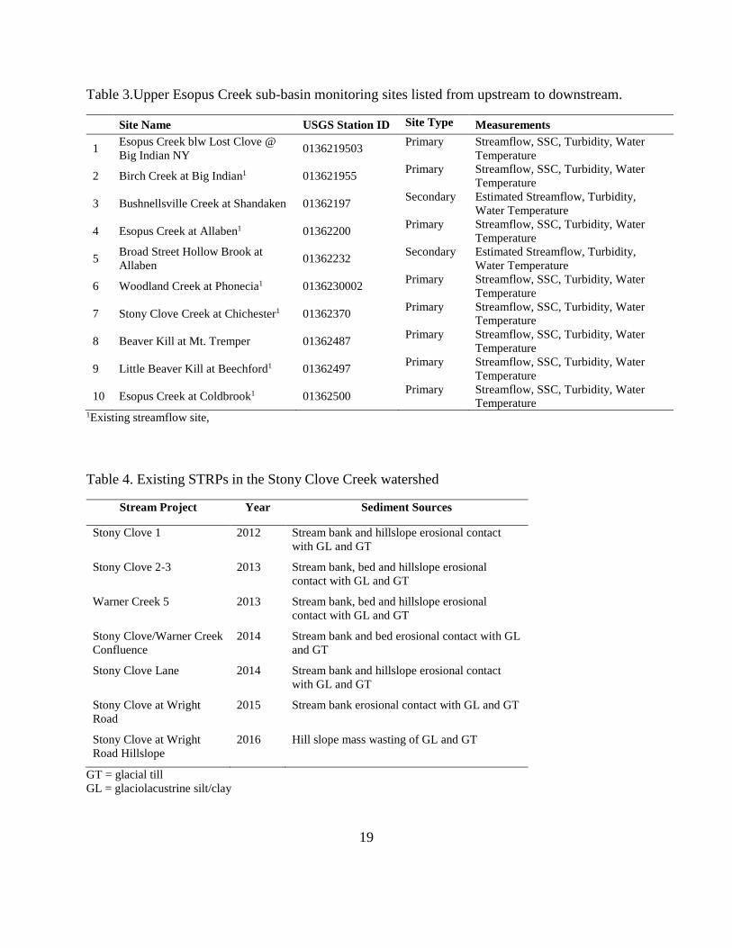
19
Table 3.Upper Esopus Creek sub-basin monitoring sites listed from upstream to downstream.
Site Name USGS Station ID Site Type Measurements
1 Esopus Creek blw Lost Clove @ Big Indian NY 0136219503 Primary Streamflow, SSC, Turbidity, Water
Temperature
2 Birch Creek at Big Indian1 013621955 Primary Streamflow, SSC, Turbidity, Water Temperature
3 Bushnellsville Creek at Shandaken 01362197 Secondary Estimated Streamflow, Turbidity, Water Temperature
4 Esopus Creek at Allaben1 01362200 Primary Streamflow, SSC, Turbidity, Water Temperature
5 Broad Street Hollow Brook at Allaben 01362232 Secondary Estimated Streamflow, Turbidity,
Water Temperature
6 Woodland Creek at Phonecia1 0136230002 Primary Streamflow, SSC, Turbidity, Water Temperature
7 Stony Clove Creek at Chichester1 01362370 Primary Streamflow, SSC, Turbidity, Water Temperature
8 Beaver Kill at Mt. Tremper 01362487 Primary Streamflow, SSC, Turbidity, Water Temperature
9 Little Beaver Kill at Beechford1 01362497 Primary Streamflow, SSC, Turbidity, Water Temperature
10 Esopus Creek at Coldbrook1 01362500 Primary Streamflow, SSC, Turbidity, Water Temperature
1Existing streamflow site,
Table 4. Existing STRPs in the Stony Clove Creek watershed
Stream Project Year Sediment Sources
Stony Clove 1 2012 Stream bank and hillslope erosional contact with GL and GT
Stony Clove 2-3 2013 Stream bank, bed and hillslope erosional contact with GL and GT
Warner Creek 5 2013 Stream bank, bed and hillslope erosional contact with GL and GT
Stony Clove/Warner Creek Confluence
2014 Stream bank and bed erosional contact with GL and GT
Stony Clove Lane 2014 Stream bank and hillslope erosional contact with GL and GT
Stony Clove at Wright Road
2015 Stream bank erosional contact with GL and GT
Stony Clove at Wright Road Hillslope
2016 Hill slope mass wasting of GL and GT
GT = glacial till GL = glaciolacustrine silt/clay
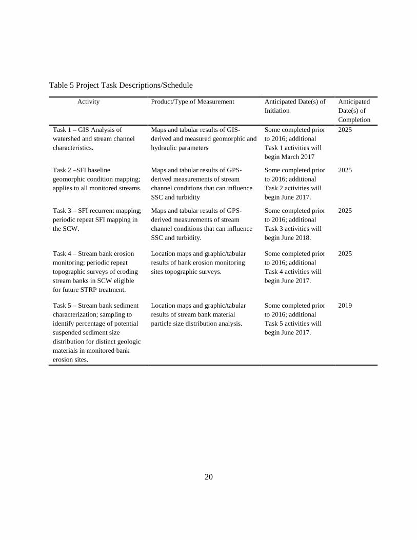
20
Table 5 Project Task Descriptions/Schedule
Activity Product/Type of Measurement Anticipated Date(s) of Initiation
Anticipated Date(s) of Completion
Task 1 – GIS Analysis of watershed and stream channel characteristics.
Maps and tabular results of GIS-derived and measured geomorphic and hydraulic parameters
Some completed prior to 2016; additional Task 1 activities will begin March 2017
2025
Task 2 –SFI baseline geomorphic condition mapping; applies to all monitored streams.
Maps and tabular results of GPS-derived measurements of stream channel conditions that can influence SSC and turbidity
Some completed prior to 2016; additional Task 2 activities will begin June 2017.
2025
Task 3 – SFI recurrent mapping; periodic repeat SFI mapping in the SCW.
Maps and tabular results of GPS-derived measurements of stream channel conditions that can influence SSC and turbidity.
Some completed prior to 2016; additional Task 3 activities will begin June 2018.
2025
Task 4 – Stream bank erosion monitoring; periodic repeat topographic surveys of eroding stream banks in SCW eligible for future STRP treatment.
Location maps and graphic/tabular results of bank erosion monitoring sites topographic surveys.
Some completed prior to 2016; additional Task 4 activities will begin June 2017.
2025
Task 5 – Stream bank sediment characterization; sampling to identify percentage of potential suspended sediment size distribution for distinct geologic materials in monitored bank erosion sites.
Location maps and graphic/tabular results of stream bank material particle size distribution analysis.
Some completed prior to 2016; additional Task 5 activities will begin June 2017.
2019
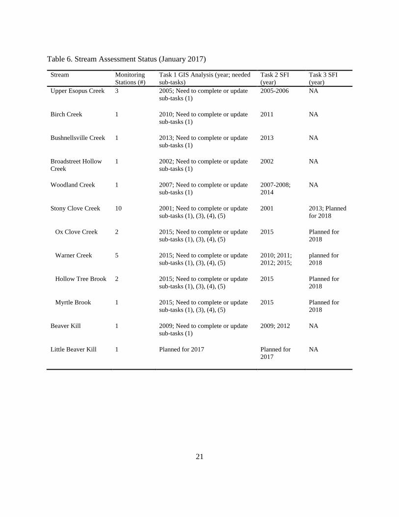
21
Table 6. Stream Assessment Status (January 2017)
Stream Monitoring Stations (#)
Task 1 GIS Analysis (year; needed sub-tasks)
Task 2 SFI (year)
Task 3 SFI (year)
Upper Esopus Creek 3 2005; Need to complete or update sub-tasks (1)
2005-2006 NA
Birch Creek 1 2010; Need to complete or update sub-tasks (1)
2011 NA
Bushnellsville Creek 1 2013; Need to complete or update sub-tasks (1)
2013 NA
Broadstreet Hollow Creek
1 2002; Need to complete or update sub-tasks (1)
2002 NA
Woodland Creek 1 2007; Need to complete or update sub-tasks (1)
2007-2008; 2014
NA
Stony Clove Creek 10 2001; Need to complete or update sub-tasks (1), (3), (4), (5)
2001 2013; Planned for 2018
Ox Clove Creek 2 2015; Need to complete or update sub-tasks (1), (3), (4), (5)
2015 Planned for 2018
Warner Creek 5 2015; Need to complete or update sub-tasks (1), (3), (4), (5)
2010; 2011; 2012; 2015;
planned for 2018
Hollow Tree Brook 2 2015; Need to complete or update sub-tasks (1), (3), (4), (5)
2015 Planned for 2018
Myrtle Brook 1 2015; Need to complete or update sub-tasks (1), (3), (4), (5)
2015 Planned for 2018
Beaver Kill 1 2009; Need to complete or update sub-tasks (1)
2009; 2012 NA
Little Beaver Kill 1 Planned for 2017 Planned for 2017
NA
22
Table 7. List of Study Variables
Variable Metrics Methods QAPP
PI
Water Quality Turbidity daily and runoff event mean value (FNU) WQ A USGS
Suspended Sediment Concentration
daily and runoff event mean value (mg/L) WQ A USGS
Suspended Sediment Load runoff event and annual value (ton) WQ, Q A USGS
Hydrology
Discharge (Daily, Storm) Mean, instantaneous peak, and duration analysis (cfs)
Q A USGS
Discharge Magnitude-Frequency
Return Period (yr) Q A USGS
Hydraulics
Stream Energy Stream power (W m-1), Unit stream power (W m-2)
H, C, G B DEP
Geomorphology
Drainage Area Drainage area (mi2) G B DEP
Erosional Process % Active Bank Hydraulic Erosion C B DEP
% Active Bank Mass Failure C B DEP
Presence of active headcuts (y/n) C B DEP
Channel/Hillslope Interaction % Channel Contact with Hillslope Processes G, C B DEP
Geology
Stream Bank Sediment Composition
% Erosional Contact Non-Alluvial Source Fine Sediment
C, S B DEP
% Erosional Contact w/ Alluvial Source Fine Sediment
C, S B DEP
Management Practices
STRP Implementation % Erosional contact with fine sediment mitigated
C, G B DEP
Methods: WQ = water quality monitoring; Q = stream discharge monitoring; H = hydraulic modeling; C = channel corridor assessment; G = GIS; S = sediment particle size analysis
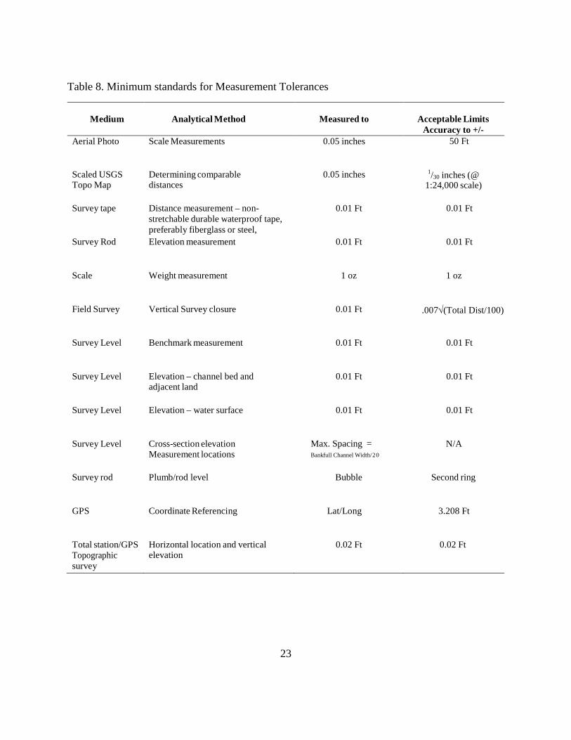
23
Table 8. Minimum standards for Measurement Tolerances
Medium
Analytical Method
Measured to
Acceptable Limits
Accuracy to +/- Aerial Photo Scale Measurements 0.05 inches 50 Ft
Scaled USGS Topo Map
Determining comparable distances
0.05 inches 1/30 inches (@ 1:24,000 scale)
Survey tape Distance measurement – non- stretchable durable waterproof tape, preferably fiberglass or steel,
0.01 Ft 0.01 Ft
Survey Rod Elevation measurement 0.01 Ft 0.01 Ft
Scale Weight measurement 1 oz 1 oz
Field Survey Vertical Survey closure 0.01 Ft .007√(Total Dist/100)
Survey Level Benchmark measurement 0.01 Ft 0.01 Ft
Survey Level Elevation – channel bed and adjacent land
0.01 Ft 0.01 Ft
Survey Level Elevation – water surface 0.01 Ft 0.01 Ft
Survey Level Cross-section elevation Measurement locations
Max. Spacing = Bankfull Channel Width/20
N/A
Survey rod Plumb/rod level Bubble Second ring
GPS Coordinate Referencing Lat/Long 3.208 Ft
Total station/GPS Topographic survey
Horizontal location and vertical elevation
0.02 Ft 0.02 Ft

24
APPENDICES Attachment A Stream Management Data Dictionary Guide Attachment B Sample Field Forms
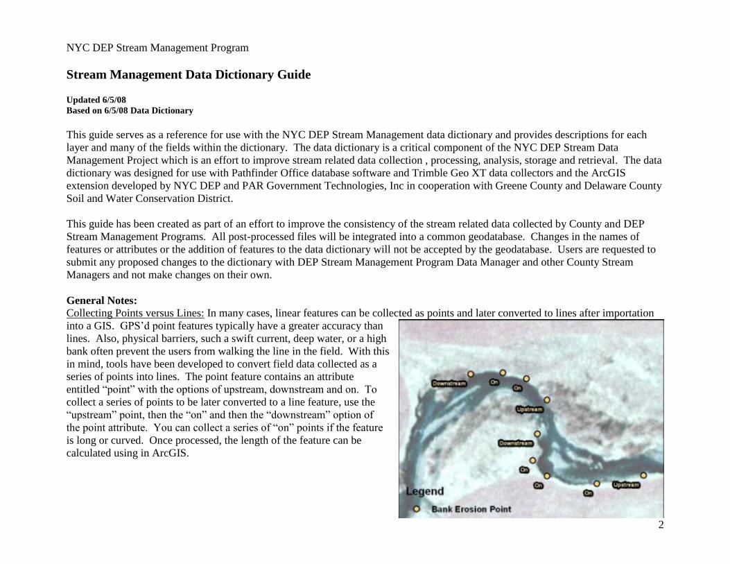
2
NYC DEP Stream Management Program
Stream Management Data Dictionary Guide Updated 6/5/08
Based on 6/5/08 Data Dictionary
This guide serves as a reference for use with the NYC DEP Stream Management data dictionary and provides descriptions for each
layer and many of the fields within the dictionary. The data dictionary is a critical component of the NYC DEP Stream Data
Management Project which is an effort to improve stream related data collection , processing, analysis, storage and retrieval. The data
dictionary was designed for use with Pathfinder Office database software and Trimble Geo XT data collectors and the ArcGIS
extension developed by NYC DEP and PAR Government Technologies, Inc in cooperation with Greene County and Delaware County
Soil and Water Conservation District.
This guide has been created as part of an effort to improve the consistency of the stream related data collected by County and DEP
Stream Management Programs. All post-processed files will be integrated into a common geodatabase. Changes in the names of
features or attributes or the addition of features to the data dictionary will not be accepted by the geodatabase. Users are requested to
submit any proposed changes to the dictionary with DEP Stream Management Program Data Manager and other County Stream
Managers and not make changes on their own.
General Notes:
Collecting Points versus Lines: In many cases, linear features can be collected as points and later converted to lines after importation
into a GIS. GPS’d point features typically have a greater accuracy than
lines. Also, physical barriers, such a swift current, deep water, or a high
bank often prevent the users from walking the line in the field. With this
in mind, tools have been developed to convert field data collected as a
series of points into lines. The point feature contains an attribute
entitled “point” with the options of upstream, downstream and on. To
collect a series of points to be later converted to a line feature, use the
“upstream” point, then the “on” and then the “downstream” option of
the point attribute. You can collect a series of “on” points if the feature
is long or curved. Once processed, the length of the feature can be
calculated using in ArcGIS.
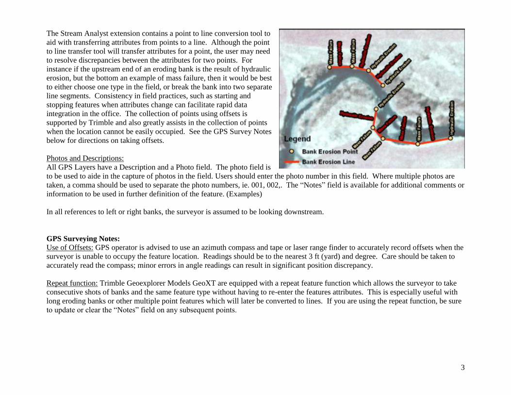
3
The Stream Analyst extension contains a point to line conversion tool to
aid with transferring attributes from points to a line. Although the point
to line transfer tool will transfer attributes for a point, the user may need
to resolve discrepancies between the attributes for two points. For
instance if the upstream end of an eroding bank is the result of hydraulic
erosion, but the bottom an example of mass failure, then it would be best
to either choose one type in the field, or break the bank into two separate
line segments. Consistency in field practices, such as starting and
stopping features when attributes change can facilitate rapid data
integration in the office. The collection of points using offsets is
supported by Trimble and also greatly assists in the collection of points
when the location cannot be easily occupied. See the GPS Survey Notes
below for directions on taking offsets.
Photos and Descriptions:
All GPS Layers have a Description and a Photo field. The photo field is
to be used to aide in the capture of photos in the field. Users should enter the photo number in this field. Where multiple photos are
taken, a comma should be used to separate the photo numbers, ie. 001, 002,. The “Notes” field is available for additional comments or
information to be used in further definition of the feature. (Examples)
In all references to left or right banks, the surveyor is assumed to be looking downstream.
GPS Surveying Notes:
Use of Offsets: GPS operator is advised to use an azimuth compass and tape or laser range finder to accurately record offsets when the
surveyor is unable to occupy the feature location. Readings should be to the nearest 3 ft (yard) and degree. Care should be taken to
accurately read the compass; minor errors in angle readings can result in significant position discrepancy.
Repeat function: Trimble Geoexplorer Models GeoXT are equipped with a repeat feature function which allows the surveyor to take
consecutive shots of banks and the same feature type without having to re-enter the features attributes. This is especially useful with
long eroding banks or other multiple point features which will later be converted to lines. If you are using the repeat function, be sure
to update or clear the “Notes” field on any subsequent points.

4
Timely Data Download: Always download, post process and bring your field data into the geodatabase as quickly as possible.
Typically you and your crew will retain familiarity with the data needed for efficient conversion for only about a week.
Know your Data Dictionary: This guide is only an introductory document. It is necessary to allow your crew a couple of days in the
field to get familiar with the data dictionary before you can expect to improve your team’s efficiency. Always check your field data in
the geodatabase and perform tests of the various conversion tasks such as converting points to lines to get a clear understanding of
proper field collection techniques.
5
Stream Management Data Dictionary Feature Index
Bank Erosion .................................................................................... Bank_P, Bank_L ...................................................... 7
BEHI ........................................................................................................ BEHI (Point) .................................................... 11
Berm ................................................................................................. Berm_P, Berm_L .................................................... 13
Best Management Practice .............................................................. BMP_P, BMP_L .................................................... 14
Bridge .................................................................................................. XBridge (Point) .................................................... 16
Control ............................................................................................. Cntrl_P, Cntrl_L .................................................... 17
Crossing ............................................................................................. Crossing (Point) .................................................... 18
Culvert .............................................................................................. XCulvert (Point) .................................................... 19
Depositional Feature ........................................................................ Dep_Feat (Point) .................................................... 20
Dump ....................................................................................................... Dump (Point) .................................................... 22
Fine Sediment Source ....................................................................... Fine_Sed (Point) .................................................... 22
Floodplain Indicator ........................................................................... Fld_Ind (Point) .................................................... 23
Gage ........................................................................................................... Gage (Point) .................................................... 24
Invasive Species ............................................................................................ InvSpp_P .................................................... 24
Land Cover .................................................................................................. LandCovP .................................................... 25
Large Woody Debris ....................................................................................... LWD_P .................................................... 28
Management Practice ...................................................................... MgtPract (Point) .................................................... 28
Monitoring Point ........................................................................................... MntrPnt .................................................... 29
Monitoring Site .................................................................................. MntrSite (Point) .................................................... 29
Montgomery and Buffington Classification ................................. ClassM_B (Point) .................................................... 30
Miscellaneous ....................................................................... Misc_P, Misc_L, Misc_A .................................................... 30
Obstruction ....................................................................................... Obstruct (Point) .................................................... 31
Pfankuch ........................................................................................................ Pfkuch_P .................................................... 32
Photo Point ...................................................................................................... Photo_P .................................................... 34
Piped Outfall ..................................................................................... PipedOut (Point) .................................................... 35
Plant Material .............................................................................................. PlantM_P .................................................... 36
Project Site ................................................................................ Project_P, Project_A .................................................... 36
Proposed Planting Site ................................................................................. PlantS_P .................................................... 37
Revetment ........................................................................................ Revet_P, Revet_L .................................................... 38
Road .................................................................................................. Road_P, Road_L .................................................... 39
Rosgen Level 1 Classification ......................................................... RosgenL1 (Point) .................................................... 40
Sediment Sample Location ............................................................ SedSample (Point) .................................................... 40
6
Site Visit ............................................................................................................ Visit_P .................................................... 41
Stream Feature ................................................................................ SFeat_P, SFeat_L .................................................... 42
Survey Control ................................................................................. SurvCont (Point) .................................................... 45
Tributary ................................................................................................... Trib (Point) .................................................... 45
Utility ....................................................................................................... Utility (Point) .................................................... 46
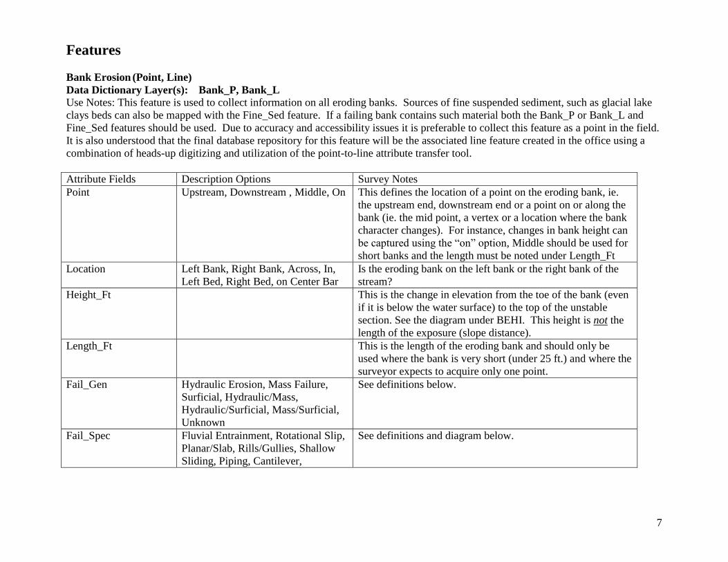
7
Features
Bank Erosion (Point, Line)
Data Dictionary Layer(s): Bank_P, Bank_L Use Notes: This feature is used to collect information on all eroding banks. Sources of fine suspended sediment, such as glacial lake
clays beds can also be mapped with the Fine_Sed feature. If a failing bank contains such material both the Bank_P or Bank_L and
Fine_Sed features should be used. Due to accuracy and accessibility issues it is preferable to collect this feature as a point in the field.
It is also understood that the final database repository for this feature will be the associated line feature created in the office using a
combination of heads-up digitizing and utilization of the point-to-line attribute transfer tool.
Attribute Fields Description Options Survey Notes
Point Upstream, Downstream , Middle, On This defines the location of a point on the eroding bank, ie.
the upstream end, downstream end or a point on or along the
bank (ie. the mid point, a vertex or a location where the bank
character changes). For instance, changes in bank height can
be captured using the “on” option, Middle should be used for
short banks and the length must be noted under Length_Ft
Location Left Bank, Right Bank, Across, In,
Left Bed, Right Bed, on Center Bar
Is the eroding bank on the left bank or the right bank of the
stream?
Height_Ft This is the change in elevation from the toe of the bank (even
if it is below the water surface) to the top of the unstable
section. See the diagram under BEHI. This height is not the
length of the exposure (slope distance).
Length_Ft This is the length of the eroding bank and should only be
used where the bank is very short (under 25 ft.) and where the
surveyor expects to acquire only one point.
Fail_Gen Hydraulic Erosion, Mass Failure,
Surficial, Hydraulic/Mass,
Hydraulic/Surficial, Mass/Surficial,
Unknown
See definitions below.
Fail_Spec Fluvial Entrainment, Rotational Slip,
Planar/Slab, Rills/Gullies, Shallow
Sliding, Piping, Cantilever,
See definitions and diagram below.
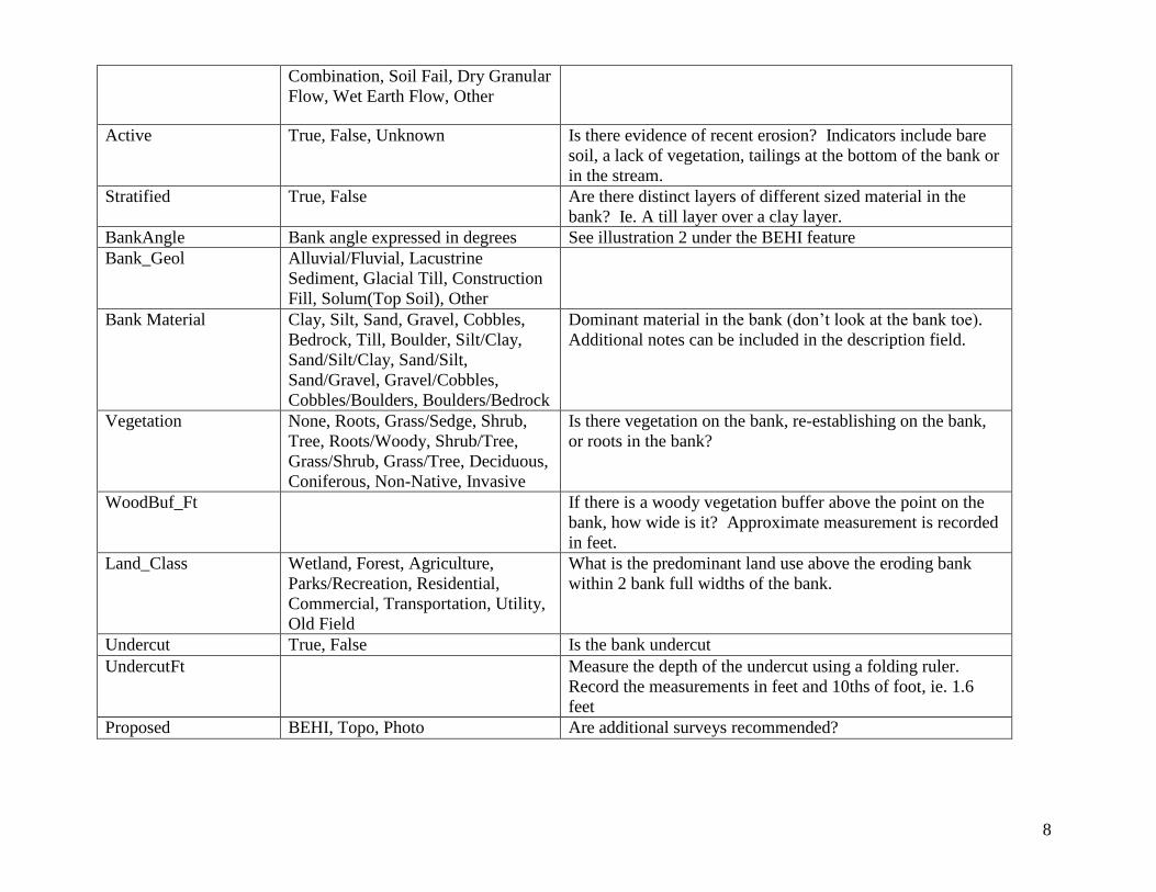
8
Combination, Soil Fail, Dry Granular
Flow, Wet Earth Flow, Other
Active True, False, Unknown Is there evidence of recent erosion? Indicators include bare
soil, a lack of vegetation, tailings at the bottom of the bank or
in the stream.
Stratified True, False Are there distinct layers of different sized material in the
bank? Ie. A till layer over a clay layer.
BankAngle Bank angle expressed in degrees See illustration 2 under the BEHI feature
Bank_Geol Alluvial/Fluvial, Lacustrine
Sediment, Glacial Till, Construction
Fill, Solum(Top Soil), Other
Bank Material Clay, Silt, Sand, Gravel, Cobbles,
Bedrock, Till, Boulder, Silt/Clay,
Sand/Silt/Clay, Sand/Silt,
Sand/Gravel, Gravel/Cobbles,
Cobbles/Boulders, Boulders/Bedrock
Dominant material in the bank (don’t look at the bank toe).
Additional notes can be included in the description field.
Vegetation None, Roots, Grass/Sedge, Shrub,
Tree, Roots/Woody, Shrub/Tree,
Grass/Shrub, Grass/Tree, Deciduous,
Coniferous, Non-Native, Invasive
Is there vegetation on the bank, re-establishing on the bank,
or roots in the bank?
WoodBuf_Ft If there is a woody vegetation buffer above the point on the
bank, how wide is it? Approximate measurement is recorded
in feet.
Land_Class Wetland, Forest, Agriculture,
Parks/Recreation, Residential,
Commercial, Transportation, Utility,
Old Field
What is the predominant land use above the eroding bank
within 2 bank full widths of the bank.
Undercut True, False Is the bank undercut
UndercutFt Measure the depth of the undercut using a folding ruler.
Record the measurements in feet and 10ths of foot, ie. 1.6
feet
Proposed BEHI, Topo, Photo Are additional surveys recommended?
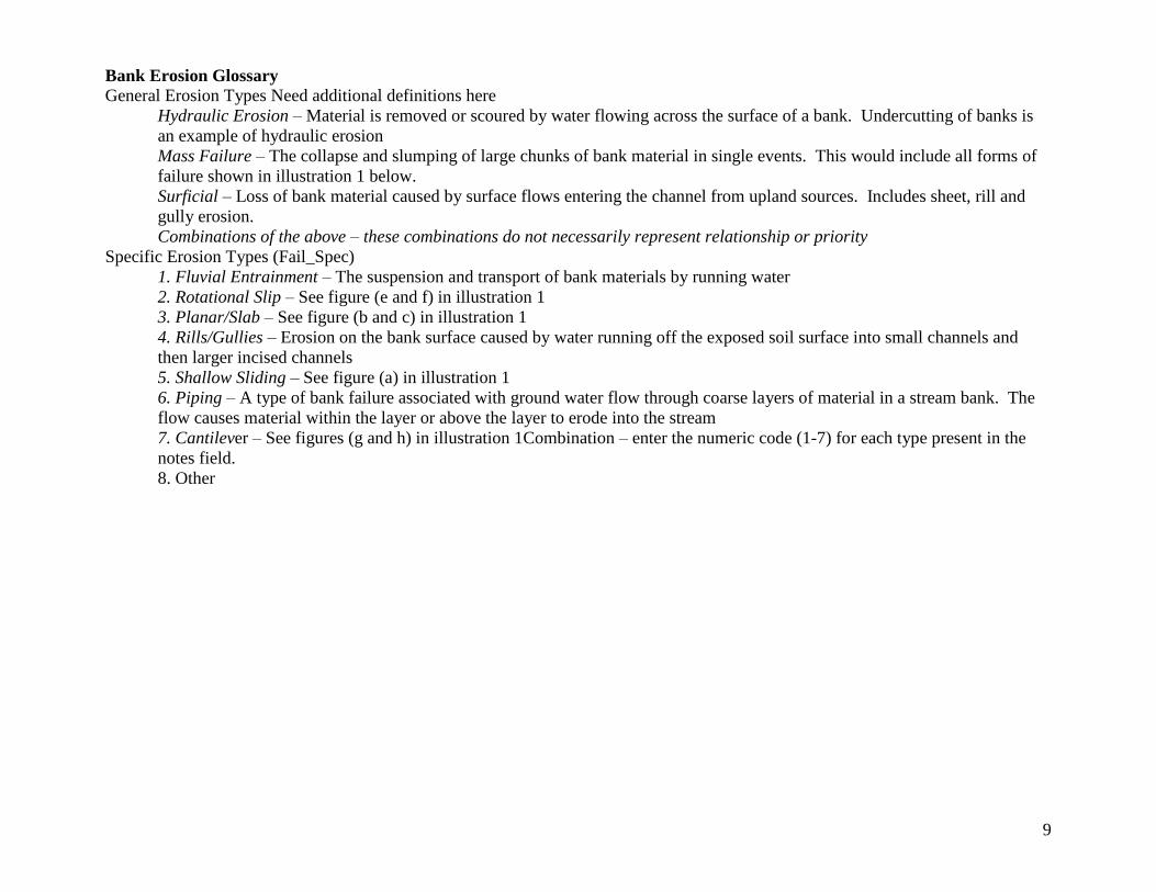
9
Bank Erosion Glossary
General Erosion Types Need additional definitions here
Hydraulic Erosion – Material is removed or scoured by water flowing across the surface of a bank. Undercutting of banks is
an example of hydraulic erosion
Mass Failure – The collapse and slumping of large chunks of bank material in single events. This would include all forms of
failure shown in illustration 1 below.
Surficial – Loss of bank material caused by surface flows entering the channel from upland sources. Includes sheet, rill and
gully erosion.
Combinations of the above – these combinations do not necessarily represent relationship or priority
Specific Erosion Types (Fail_Spec)
1. Fluvial Entrainment – The suspension and transport of bank materials by running water
2. Rotational Slip – See figure (e and f) in illustration 1
3. Planar/Slab – See figure (b and c) in illustration 1
4. Rills/Gullies – Erosion on the bank surface caused by water running off the exposed soil surface into small channels and
then larger incised channels
5. Shallow Sliding – See figure (a) in illustration 1
6. Piping – A type of bank failure associated with ground water flow through coarse layers of material in a stream bank. The
flow causes material within the layer or above the layer to erode into the stream
7. Cantilever – See figures (g and h) in illustration 1Combination – enter the numeric code (1-7) for each type present in the
notes field.
8. Other
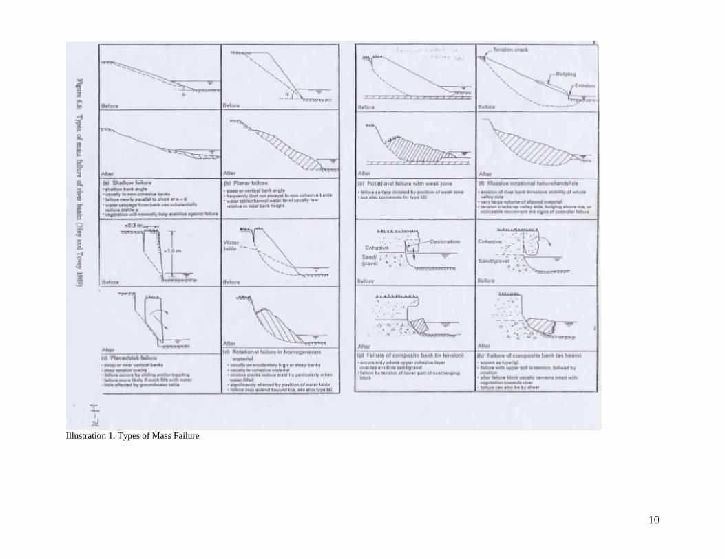
10
Illustration 1. Types of Mass Failure
11
BEHI (Point)
Data Dictionary Layer(s): BEHI
Use Notes: This layer is used identify the location and could be used to capture information gathered from a Bank Erosion Hazard
Index survey. Sites where a future BEHI survey is recommended should be identified in the Bank Erosion feature. The BEHI survey
protocol as described by D. Rosgen should be followed when taking measurements. While the data dictionary provides attributes to
capture the entire set of BEHI variables, information from field forms, PocketRivermorph, or total station surveys can be integrated
with the basic point information (id, data and location) within the geodatabase.
Attribute Fields Description Options Survey Note
BEHI_ID Identification number
BEHI_Date Date of BEHI survey, Month/Day/Year
Location Left Bank, Right Bank
BkFl_HtFt Bankfull Height Ft See illustration 2
Bk_Ht_Ft Bank Height Ft See illustration 2
RootDpthFt Root Depth Ft See illustration 2
pctRootDen Root Density % See illustration 2
Bank_Angle degrees See illustration 2
pctCover Surface Protection Percentage of surface covered by vegetation or other
BkankLngth Bank Length Ft Length of the eroding bank
BankMatrl Size material
Bank_Strat See glossary
Strat_Sev 1,2,3,4,5 One lowest, five highest
BEHI Glossary:
BEHI – Bank Erosion Hazard Index, as developed by D. Rosgen 1996, is a descriptor of bank condition and can be used to predict
erosion potential.
Bankfull Height – For BEHI the bankfull height is the difference in elevation from the deepest point in the channel at the toe of the
bank to the bankfull elevation (B in diagram 1)
Bank Height – Total height of the bank (A in illustration 2
Root Dpth Ft – Depth of roots from the top of the bank (C in illustration)
pctRootDen – Estimate of volume filled by roots
pctCover – Estimate of surface covered by vegetation
Bank Length – This can be estimated or taken from the bank erosion feature in the GIS
12
Reach Length – This can be acquired from the GIS
BankMatrl – Bedrock, Boulders, Cobble, Gravel, Sand, Silt/Clay
Bank_Strat - Presence, extent, sequence and position of stratification relative to bankful elevation
Strat_Sev – rating
Illustration 2. BEHI Variables from Rosgen
13
Berm (Point, Line)
Data Dictionary Layer(s): Berm_P, Berm_L
Use Notes: Due to accuracy and accessibility issues it is preferable to collect this feature as a point in the field. It is also understood
that the final database repository for this feature will be the associated line feature created in the office using a combination of heads-
up digitizing and utilization of the point-to-line attribute transfer tool
Attribute Fields Description Options Survey Notes
Point Upstream,Downstream, On This defines the location of point on the eroding bank, ie. the
upstream end, a point on the bank, or the downstream end.
Changes in berm characteristics can be captured using the “on”
option
Location LB, RB Is it on the left or the right bank?
Avg Ht_Ft Average Height (ft.) Height of the top of the berm above the surrounding floodplain.
Height should be measured as the change in elevation, not slope
distance.
Avg Wid_Ft Average Width (ft.) As measured at the base of the berm in feet.
Vegetation None, Grass/Sedge, Shrub,
Roots/Woody
Is there vegetation on the berm?
Activity True, False Is this an actively maintained berm?
Material
Boulder, Stone, Log, Concrete,
Sheet Piling, Bedrock, Earthen,
Other
From what you can detect, what is the principal material used to
construct the berm?
Berm Glossary:
Berm – a manmade structure constructed to confine flood flows.
14
Best Management Practice (Point,Line)
Data Dictionary Layer(s): BMP_P, BMP_L
Use Notes: This feature is used to map the location of best management practices such as natural channel design structures,
bioengineering, or other practices advanced by stream managers. Due to accuracy and accessibility issues it is preferable to collect
this feature as a point in the field. It is also understood that the final database repository for this feature will be the associated line
feature created in the office using a combination of heads-up digitizing and utilization of the point-to-line attribute transfer tool
Attribute field Description Options Survey Notes
Point Upstream, Downstream, On,
Middle
Location Left Bank, Right Bank, Across, In,
Thalweg
BMP_Type Vane, Cross Vane, Weir, Root
Wad, Fascine, VRSS, Live Stakes,
Live Crib, Joint Planting, Coconut
Roll, Tree Seedling, Hydroseeded,
Other
See definitions below
Material Rock, Log , Plant, Other
FunctCond Good, Fair, Poor, Not Functional Good – flows directed away from bank, no signs of bank stress,
pool depth adequate but not excessive
Fair – some bank or bed scour, flow may not be moving through the
proper point on the structure, possibly some aggradation in the pool.
Poor – significant bed or bank scour, aggradation, or flow is
misdirected or beginning to move around the structure.
Not Functional – structure is not redirecting flow away from the
bank or protecting the bed, in fact excessive scour may be causing
the channel to migrate.
StructCond New, Good, Fair, Poor, Failed New – the structure is new and has not experienced a bankfull event
Good – the structure has experienced bankfull events and still
appears much the same as when constructed.
Fair – the structure has deteriorated and may be missing stones,
may have gaps, settled or rotated materials, failed support plantings,
may show evidence of the scour or aggradation.
15
Poor – the structure is crumbling, slumping, covered with sediment,
scoured out, show evidence of the significant likelihood that failure
can be expected in the near future.
Failed – the structure has been significantly damaged. Ie. it has
been washed away, buried, or no longer flows
Length_Ft Required when “middle” is selected on the point option
Vane – Rock or wood structures that protrude from either streambank, angled upstream, but does not extend entirely across a channel.
They deflect flows away from the bank, and dissipate energy in downstream scour pools created by water flowing over the vane.
Cross Vane – see Weir Log, boulder, or quarrystone structures placed across the channel and keyed into the streambank to control
grade, dissipate energy, create pool habitat, control bed erosion.
Weir – a log, stone or concrete structure protruding from either streambank used to deflect flow
Root Wad – a tree root mass keyed into the bank with boulders or quarrystone to provide energy dissipation, and create habitat.
Fascine – Long bundles of woody branches partially buried to provide as a means of establishing rows of regeneration for bank and
floodplain protection
VRSS – Vegetated Reinforces Slope Stablization, a bioengineering practice which combines brush layering and geotextile materials to
secure soil in layers on steep, high embankments
Live Cribbing – the use of vigorously sprouting woody materials stacked and backfilled to produce a living bank protection structure.
Live Staking – use of woody cuttings partially buried along a bank or floodplain for the purpose of establishing new trees or shrubs
Joint Planting – live staking or potted plant material planted in the cracks or interspaces of riprap or stacked rock walls for the purpose
of providing long term bank stability and improved habitat.
Coconut Roll – A roll or log of flexible coconut fiber used in bank stabilization and bioengineering practices
Tree Seedlings – An indication that tree seedlings were planted in the area of the point
Hydroseeded – An indication that hydroseeding was used to stabilize an area following a disturbance
16
Bridge (Point)
Data Dictionary Layer(s): Bridge
Use Notes: Indicated the location of a bridge. The point should be taken on the bridge center or where the bridge crosses the stream.
Attribute Fields Description Options Survey Notes
Owner Private, County, State, Town,
Village
Bridge_ID Id number is commonly displayed on the abutment under the bridge
deck
Road_Name Name of road
SpanNormFt Span from abutment to abutment
SpanEffect Span that actually conveys the flow
Ht_Ft Average height from bottom of deck to the stream bed
Funct Conveying, Contributing Does the bridge cross the main stem (conveying) or a tributary
(contributing)
FunctCond Good, Fair, Poor, Not Functioning Good – flows received and directed as intended by the structure
Fair – some excessive bank or bed scour, flow may not be moving
through the proper point on the structure, possibly some
aggradation above or degradation below.
Poor – significant bed or bank scour above or below, aggradation
above or below, or flow is misdirected. Flow is beginning to move
undermine the piers or abuttments. Debris collects easily.
Not Functioning – structure is not controlling the flow. The channel
is routed around the bridge.
StructCond New, Good, Fair, Poor, Failed New – the structure is new and may not have experienced a flood
event
Good – the structure has experienced bankfull events and still
appears much the same as when constructed.
Fair – the bridge has deteriorated and may be corroded, scour or
erosion of abutments or piers. May show evidence significant age
Poor – the structure is crumbling or collapsing etc.
Failed – blown out, collapsed
Piers Number of Piers supporting the bridge
17
Encroch_Rt Number of Ft. encroachment of the right abutment on the right
floodplain
Encroch_Lf Number of Ft. encroachment of the left abutment on the left bank
Bridge Glossary:
SpanEffect – the effective portion of the span (length of opening) of the bridge which discounts portions of the span where the
direction of the flow conflicts or impeded by the abutments or piers of the bridge.
Control (Point, Line)
Data Dictionary Layer(s): Cntrl_P, Cntrl_L
Use Notes: This feature should be used to locate both grade and laterial controls either natural or man-made. Beaver dams are not
considered grade control and are entered under the Obstruction feature. Stream BMPs, that have a control function such as vanes and
cross vanes, should also be documented under BMP. Due to accuracy and accessibility issues it is preferable to collect this feature as
a point in the field. It is also understood that the final database repository for this feature will be the associated line feature created in
the office using a combination of heads-up digitizing and utilization of the point-to-line attribute transfer tool
Attribute Fields Description Options Survey Notes
Point Upstream, Downstream,
Middle, On
Location Across, Left Bed, Right
Bed, Left Bank, Right
Bank, All
If more than one type exists, ie. left bed and left bank, establish two separate
points, one bed-grade control, a second as bank-planform control. “All”
denotes both left bank, bed and right bank control exists
Ctrl_Type Grade, Planform, Both
Material Boulder, Stone, Log,
Concrete, Sheet Piling,
Bedrock, Other
“Boulder” would pertain to a substantial natural control whereas “stone”
refers to a man-made structure that acts as a control.
Func_Cond Good, Fair, Poor, Not
Functioning
Relevant for man-made structures (check dams, weirs, deflectors)
Good – flows directed as intended by the structure
Fair – some excessive bank or bed scour, flow may not be moving through
the proper point on the structure, possibly some aggradation in the pool.
Poor – significant bed or bank scour, aggradation, or flow is misdirected or
beginning to move around the structure.
Not Functioning – structure is not controlling the flow. The channel is
18
beginning to migrate or headcut.
Struc_Cond New, Good, Fair, Poor,
Failed
Relevant for man-made structures (check dams, weirs, deflectors)
New – the structure is new and has not experienced a bankfull event
Good – the structure has experienced bankfull events and still appears much
the same as when constructed.
Fair – the structure has deteriorated and may be missing stones, may have
gaps, settled or rotated materials, failed support plantings, may show evidence
of the scour or aggradation.
Poor – the structure is crumbling,
Length_Ft. For use only with point “middle” option where the length of the control is
less than 25 ft long
Grade Control Glossary:
Crossing (Point)
Data Dictionary Layer(s): Crossing
Use Notes: The feature is used to capture stream crossings such as fords (crossings other than bridges and culverts). The point should
be taken in the thalweg.
Attribute field Description Options Survey Notes
CrossType Agricultural, Forestry,
Recreational, Other
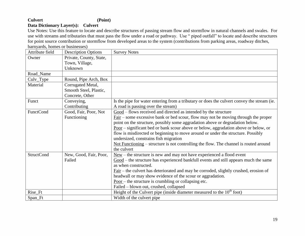
19
Culvert (Point)
Data Dictionary Layer(s): Culvert
Use Notes: Use this feature to locate and describe structures of passing stream flow and stormflow in natural channels and swales. For
use with streams and tributaries that must pass the flow under a road or pathway. Use “ piped outfall” to locate and describe structures
for point source contribution or stormflow from developed areas to the system (contributions from parking areas, roadway ditches,
barnyards, homes or businesses)
Attribute field Description Options Survey Notes
Owner Private, County, State,
Town, Village,
Unknown
Road_Name
Culv_Type Round, Pipe Arch, Box
Material Corrugated Metal,
Smooth Steel, Plastic,
Concrete, Other
Funct Conveying,
Contributing
Is the pipe for water entering from a tributary or does the culvert convey the stream (ie.
A road is passing over the stream)
FunctCond Good, Fair, Poor, Not
Functioning
Good – flows received and directed as intended by the structure
Fair – some excessive bank or bed scour, flow may not be moving through the proper
point on the structure, possibly some aggradation above or degradation below.
Poor – significant bed or bank scour above or below, aggradation above or below, or
flow is misdirected or beginning to move around or under the structure. Possibly
undersized, constrains fish migration
Not Functioning – structure is not controlling the flow. The channel is routed around
the culvert
StructCond New, Good, Fair, Poor,
Failed
New – the structure is new and may not have experienced a flood event
Good – the structure has experienced bankfull events and still appears much the same
as when constructed.
Fair – the culvert has deteriorated and may be corroded, slightly crushed, erosion of
headwall or may show evidence of the scour or aggradation.
Poor – the structure is crumbling or collapsing etc.
Failed – blown out, crushed, collapsed
Rise_Ft Height of the Culvert pipe (inside diameter measured to the 10th
foot)
Span_Ft Width of the culvert pipe
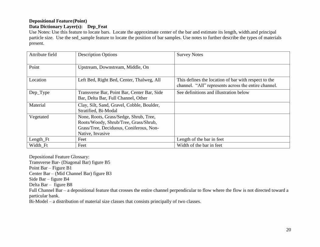
20
Depositional Feature (Point)
Data Dictionary Layer(s): Dep_Feat
Use Notes: Use this feature to locate bars. Locate the approximate center of the bar and estimate its length, width.and principal
particle size. Use the sed_sample feature to locate the position of bar samples. Use notes to further describe the types of materials
present.
Attribute field Description Options Survey Notes
Point Upstream, Downstream, Middle, On
Location Left Bed, Right Bed, Center, Thalweg, All This defines the location of bar with respect to the
channel. “All” represents across the entire channel.
Dep_Type Transverse Bar, Point Bar, Center Bar, Side
Bar, Delta Bar, Full Channel, Other
See definitions and illustration below
Material Clay, Silt, Sand, Gravel, Cobble, Boulder,
Stratified, Bi-Modal
Vegetated None, Roots, Grass/Sedge, Shrub, Tree,
Roots/Woody, Shrub/Tree, Grass/Shrub,
Grass/Tree, Deciduous, Coniferous, Non-
Native, Invasive
Length_Ft Feet Length of the bar in feet
Width_Ft Feet Width of the bar in feet
Depositional Feature Glossary:
Transverse Bar- (Diagonal Bar) figure B5
Point Bar – Figure B1
Center Bar – (Mid Channel Bar) figure B3
Side Bar – figure B4
Delta Bar – figure B8
Full Channel Bar – a depositional feature that crosses the entire channel perpendicular to flow where the flow is not directed toward a
particular bank.
Bi-Model – a distribution of material size classes that consists principally of two classes.
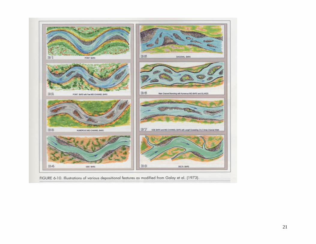
21
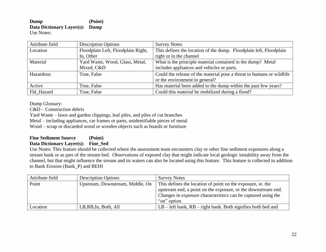
22
Dump (Point)
Data Dictionary Layer(s): Dump
Use Notes:
Attribute field Description Options Survey Notes
Location Floodplain Left, Floodplain Right,
In, Other
This defines the location of the dump. Floodplain left, Floodplain
right or in the channel
Material Yard Waste, Wood, Glass, Metal,
Mixed, C&D
What is the principle material contained in the dump? Metal
includes appliances and vehicles or parts.
Hazardous True, False Could the release of the material pose a threat to humans or wildlife
or the environment in general?
Active True, False Has material been added to the dump within the past few years?
Fld_Hazard True, False Could this material be mobilized during a flood?
Dump Glossary:
C&D – Construction debris
Yard Waste – lawn and garden clippings, leaf piles, and piles of cut branches
Metal – including appliances, car frames or parts, unidentifiable pieces of metal
Wood – scrap or discarded wood or wooden objects such as boards or furniture
Fine Sediment Source (Point)
Data Dictionary Layer(s): Fine_Sed
Use Notes: This feature should be collected where the assessment team encounters clay or other fine sediment exposures along a
stream bank or as part of the stream bed. Observations of exposed clay that might indicate local geologic instability away from the
channel, but that might influence the stream and its waters can also be located using this feature. This feature is collected in addition
to Bank Erosion (Bank_P) and BEHI
Attribute field Description Options Survey Notes
Point Upstream, Downstream, Middle, On This defines the location of point on the exposure, ie. the
upstream end, a point on the exposure, or the downstream end.
Changes in exposure characteristics can be captured using the
“on” option
Location LB,RB,In, Both, All LB – left bank, RB – right bank. Both signifies both bed and
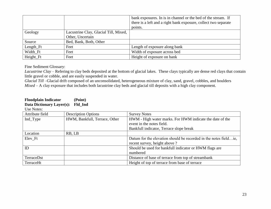
23
bank exposures. In is in channel or the bed of the stream. If
there is a left and a right bank exposure, collect two separate
points.
Geology Lacustrine Clay, Glacial Till, Mixed,
Other, Uncertain
Source Bed, Bank, Both, Other
Length_Ft Feet Length of exposure along bank
Width_Ft Feet Width of exposure across bed
Height_Ft Feet Height of exposure on bank
Fine Sediment Glossary:
Lacustrine Clay – Refering to clay beds deposited at the bottom of glacial lakes. These clays typically are dense red clays that contain
little gravel or cobble, and are easily suspended in water.
Glacial Till –Glacial drift composed of an unconsolidated, heterogeneous mixture of clay, sand, gravel, cobbles, and boulders
Mixed – A clay exposure that includes both lacustrine clay beds and glacial till deposits with a high clay component.
Floodplain Indicator (Point)
Data Dictionary Layer(s): Fld_Ind
Use Notes:
Attribute field Description Options Survey Notes
Ind_Type HWM, Bankfull, Terrace, Other HWM - High water marks. For HWM indicate the date of the
event in the notes field.
Bankfull indicator, Terrace slope break
Location RB, LB
Elev_Ft Datum for the elevation should be recorded in the notes field…ie,
recent survey, height above ?
ID Should be used for bankfull indicator or HWM flags are
numbered
TerraceDst Distance of base of terrace from top of streambank
TerraceHt Height of top of terrace from base of terrace
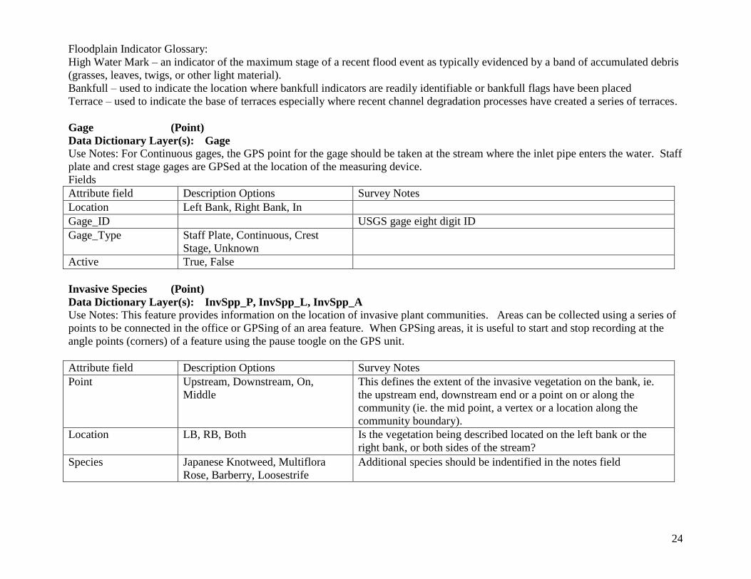
24
Floodplain Indicator Glossary:
High Water Mark – an indicator of the maximum stage of a recent flood event as typically evidenced by a band of accumulated debris
(grasses, leaves, twigs, or other light material).
Bankfull – used to indicate the location where bankfull indicators are readily identifiable or bankfull flags have been placed
Terrace – used to indicate the base of terraces especially where recent channel degradation processes have created a series of terraces.
Gage (Point)
Data Dictionary Layer(s): Gage
Use Notes: For Continuous gages, the GPS point for the gage should be taken at the stream where the inlet pipe enters the water. Staff
plate and crest stage gages are GPSed at the location of the measuring device.
Fields
Attribute field Description Options Survey Notes
Location Left Bank, Right Bank, In
Gage_ID USGS gage eight digit ID
Gage_Type Staff Plate, Continuous, Crest
Stage, Unknown
Active True, False
Invasive Species (Point)
Data Dictionary Layer(s): InvSpp_P, InvSpp_L, InvSpp_A
Use Notes: This feature provides information on the location of invasive plant communities. Areas can be collected using a series of
points to be connected in the office or GPSing of an area feature. When GPSing areas, it is useful to start and stop recording at the
angle points (corners) of a feature using the pause toogle on the GPS unit.
Attribute field Description Options Survey Notes
Point Upstream, Downstream, On,
Middle
This defines the extent of the invasive vegetation on the bank, ie.
the upstream end, downstream end or a point on or along the
community (ie. the mid point, a vertex or a location along the
community boundary).
Location LB, RB, Both Is the vegetation being described located on the left bank or the
right bank, or both sides of the stream?
Species Japanese Knotweed, Multiflora
Rose, Barberry, Loosestrife
Additional species should be indentified in the notes field
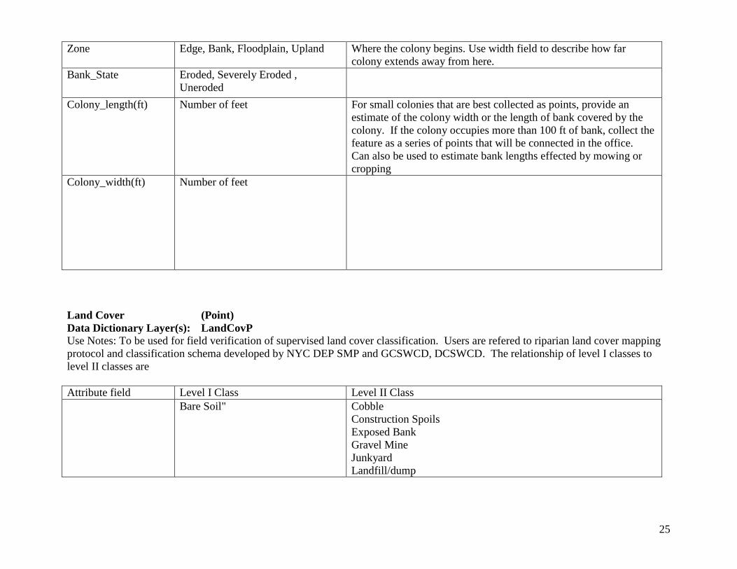
25
Zone Edge, Bank, Floodplain, Upland Where the colony begins. Use width field to describe how far
colony extends away from here.
Bank_State Eroded, Severely Eroded ,
Uneroded
Colony_length(ft) Number of feet For small colonies that are best collected as points, provide an
estimate of the colony width or the length of bank covered by the
colony. If the colony occupies more than 100 ft of bank, collect the
feature as a series of points that will be connected in the office.
Can also be used to estimate bank lengths effected by mowing or
cropping
Colony_width(ft) Number of feet
Land Cover (Point)
Data Dictionary Layer(s): LandCovP
Use Notes: To be used for field verification of supervised land cover classification. Users are refered to riparian land cover mapping
protocol and classification schema developed by NYC DEP SMP and GCSWCD, DCSWCD. The relationship of level I classes to
level II classes are
Attribute field Level I Class Level II Class
Bare Soil"
Cobble
Construction Spoils
Exposed Bank
Gravel Mine
Junkyard
Landfill/dump
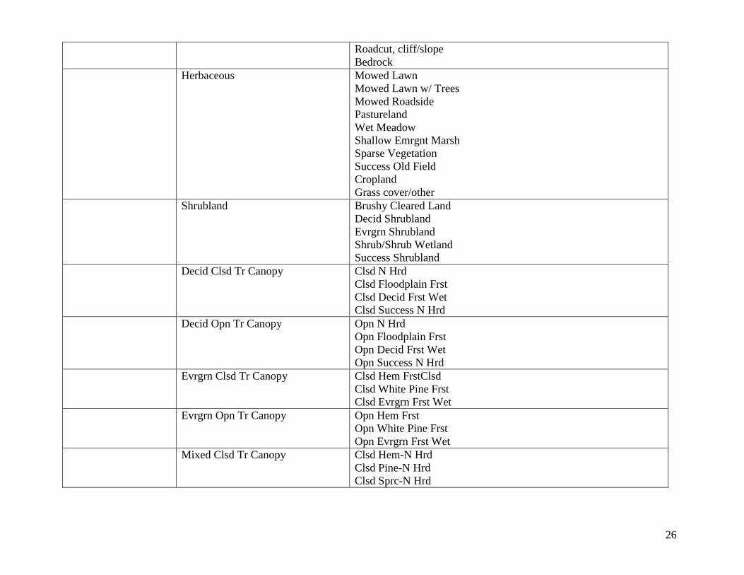
26
Roadcut, cliff/slope
Bedrock
Herbaceous Mowed Lawn
Mowed Lawn w/ Trees
Mowed Roadside
Pastureland
Wet Meadow
Shallow Emrgnt Marsh
Sparse Vegetation
Success Old Field
Cropland
Grass cover/other
Shrubland Brushy Cleared Land
Decid Shrubland
Evrgrn Shrubland
Shrub/Shrub Wetland
Success Shrubland
Decid Clsd Tr Canopy Clsd N Hrd
Clsd Floodplain Frst
Clsd Decid Frst Wet
Clsd Success N Hrd
Decid Opn Tr Canopy Opn N Hrd
Opn Floodplain Frst
Opn Decid Frst Wet
Opn Success N Hrd
Evrgrn Clsd Tr Canopy Clsd Hem FrstClsd
Clsd White Pine Frst
Clsd Evrgrn Frst Wet
Evrgrn Opn Tr Canopy Opn Hem Frst
Opn White Pine Frst
Opn Evrgrn Frst Wet
Mixed Clsd Tr Canopy Clsd Hem-N Hrd
Clsd Pine-N Hrd
Clsd Sprc-N Hrd
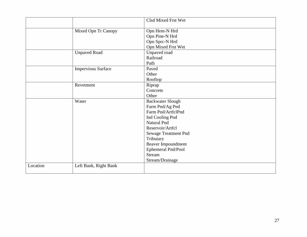
27
Clsd Mixed Frst Wet
Mixed Opn Tr Canopy Opn Hem-N Hrd
Opn Pine-N Hrd
Opn Sprc-N Hrd
Opn Mixed Frst Wet
Unpaved Road Unpaved road
Railroad
Path
Impervious Surface Paved
Other
Rooftop
Revetment Riprap
Concrete
Other
Water Backwater Slough
Farm Pnd/Ag Pnd
Farm Pnd/ArtfclPnd
Ind Cooling Pnd
Natural Pnd
Reservoir/Artfcl
Sewage Treatment Pnd
Tributary
Beaver Impoundment
Ephemeral Pnd/Pool
Stream
Stream/Drainage
Location Left Bank, Right Bank
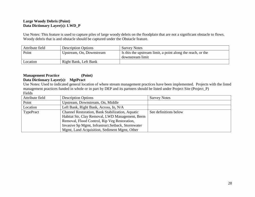
28
Large Woody Debris (Point)
Data Dictionary Layer(s): LWD_P
Use Notes: This feature is used to capture piles of large woody debris on the floodplain that are not a significant obstacle to flows.
Woody debris that is and obstacle should be captured under the Obstacle feature.
Attribute field Description Options Survey Notes
Point Upstream, On, Downstream Is this the upstream limit, a point along the reach, or the
downstream limit
Location Right Bank, Left Bank
Management Practice (Point)
Data Dictionary Layer(s): MgtPract
Use Notes: Used to indicated general location of where stream management practices have been implemented. Projects with the listed
management practices funded in whole or in part by DEP and its partners should be listed under Project Site (Project_P)
Fields
Attribute field Description Options Survey Notes
Point Upstream, Downstream, On, Middle
Location Left Bank, Right Bank, Across, In, N/A
TypePract Channel Restoration, Bank Stabilization, Aquatic
Habitat Str, Clay Removal, LWD Management, Berm
Removal, Flood Control, Rip Veg Restoration,
Invasive Sp Mgmt, Infrastruct.Setback, Stormwater
Mgmt, Land Acquisition, Sediment Mgmt, Other
See definitions below
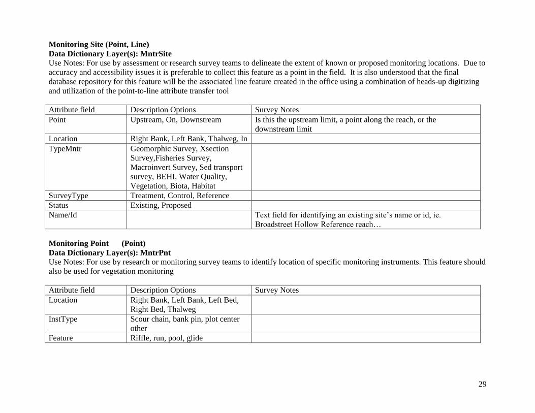
29
Monitoring Site (Point, Line)
Data Dictionary Layer(s): MntrSite
Use Notes: For use by assessment or research survey teams to delineate the extent of known or proposed monitoring locations. Due to
accuracy and accessibility issues it is preferable to collect this feature as a point in the field. It is also understood that the final
database repository for this feature will be the associated line feature created in the office using a combination of heads-up digitizing
and utilization of the point-to-line attribute transfer tool
Attribute field Description Options Survey Notes
Point Upstream, On, Downstream Is this the upstream limit, a point along the reach, or the
downstream limit
Location Right Bank, Left Bank, Thalweg, In
TypeMntr Geomorphic Survey, Xsection
Survey,Fisheries Survey,
Macroinvert Survey, Sed transport
survey, BEHI, Water Quality,
Vegetation, Biota, Habitat
SurveyType Treatment, Control, Reference
Status Existing, Proposed
Name/Id Text field for identifying an existing site’s name or id, ie.
Broadstreet Hollow Reference reach…
Monitoring Point (Point)
Data Dictionary Layer(s): MntrPnt
Use Notes: For use by research or monitoring survey teams to identify location of specific monitoring instruments. This feature should
also be used for vegetation monitoring
Attribute field Description Options Survey Notes
Location Right Bank, Left Bank, Left Bed,
Right Bed, Thalweg
InstType Scour chain, bank pin, plot center
other
Feature Riffle, run, pool, glide
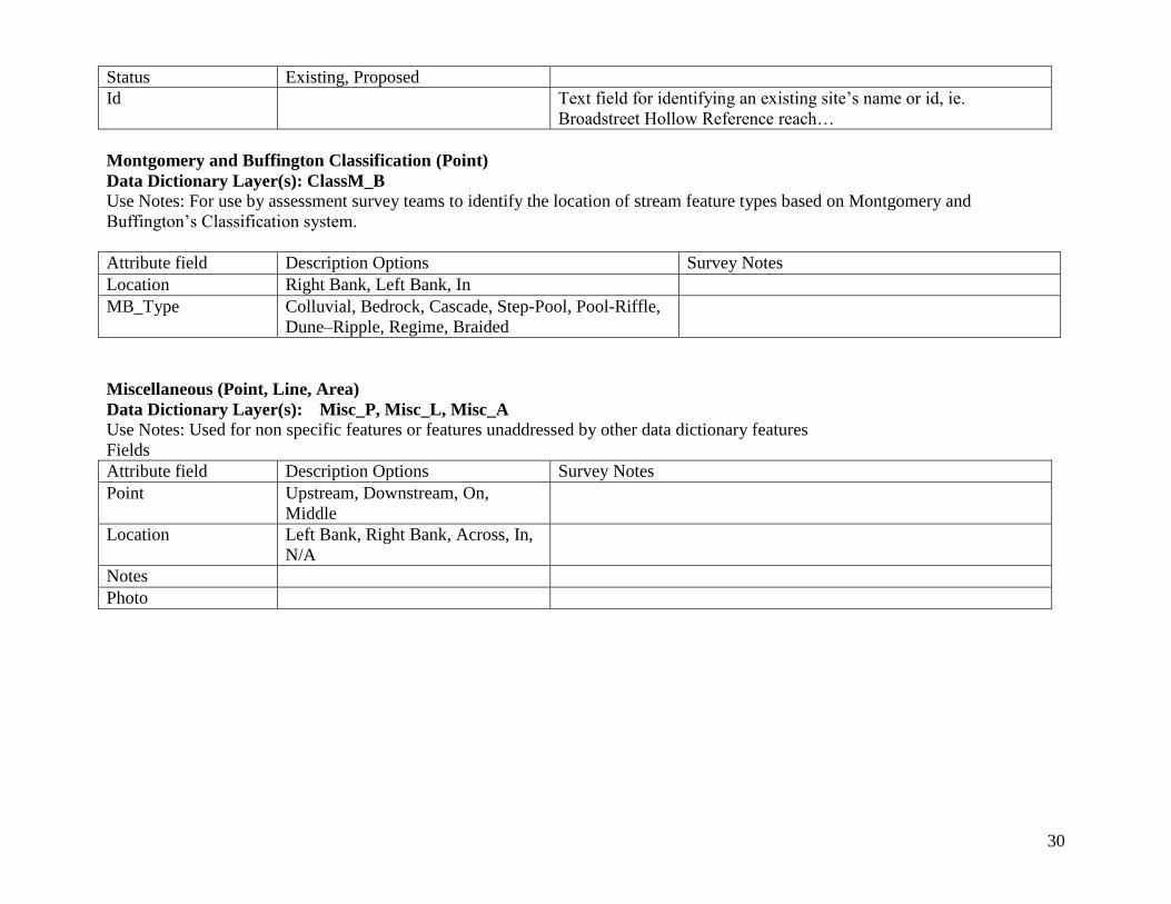
30
Status Existing, Proposed
Id Text field for identifying an existing site’s name or id, ie.
Broadstreet Hollow Reference reach…
Montgomery and Buffington Classification (Point)
Data Dictionary Layer(s): ClassM_B
Use Notes: For use by assessment survey teams to identify the location of stream feature types based on Montgomery and
Buffington’s Classification system.
Attribute field Description Options Survey Notes
Location Right Bank, Left Bank, In
MB_Type Colluvial, Bedrock, Cascade, Step-Pool, Pool-Riffle,
Dune–Ripple, Regime, Braided
Miscellaneous (Point, Line, Area)
Data Dictionary Layer(s): Misc_P, Misc_L, Misc_A
Use Notes: Used for non specific features or features unaddressed by other data dictionary features
Fields
Attribute field Description Options Survey Notes
Point Upstream, Downstream, On,
Middle
Location Left Bank, Right Bank, Across, In,
N/A
Notes
Photo
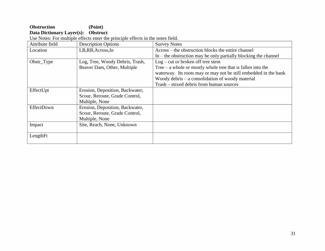
31
Obstruction (Point)
Data Dictionary Layer(s): Obstruct
Use Notes: For multiple effects enter the principle effects in the notes field.
Attribute field Description Options Survey Notes
Location LB,RB,Across,In Across – the obstruction blocks the entire channel
In – the obstruction may be only partially blocking the channel
Obstr_Type Log, Tree, Woody Debris, Trash,
Beaver Dam, Other, Multiple
Log – cut or broken off tree stem
Tree – a whole or mostly whole tree that is fallen into the
waterway. Its roots may or may not be still embedded in the bank
Woody debris – a consolidation of woody material
Trash – mixed debris from human sources
EffectUpt Erosion, Deposition, Backwater,
Scour, Reroute, Grade Control,
Multiple, None
EffectDown Erosion, Deposition, Backwater,
Scour, Reroute, Grade Control,
Multiple, None
Impact Site, Reach, None, Unknown
LengthFt
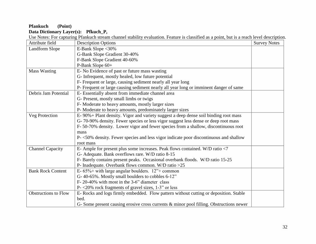
32
Pfankuch (Point)
Data Dictionary Layer(s): Pfkuch_P,
Use Notes: For capturing Pfankuch stream channel stability evaluation. Feature is classified as a point, but is a reach level description.
Attribute field Description Options Survey Notes
Landform Slope E-Bank Slope <30%
G-Bank Slope Gradient 30-40%
F-Bank Slope Gradient 40-60%
P-Bank Slope 60+
Mass Wasting E- No Evidence of past or future mass wasting
G- Infrequent, mostly healed, low future potential
F- Frequent or large, causing sediment nearly all year long
P- Frequent or large causing sediment nearly all year long or imminent danger of same
Debris Jam Potential E- Essentially absent from immediate channel area
G- Present, mostly small limbs or twigs
F- Moderate to heavy amounts, mostly larger sizes
P- Moderate to heavy amounts, predominately larger sizes
Veg Protection E- 90%+ Plant density. Vigor and variety suggest a deep dense soil binding root mass
G- 70-90% density. Fewer species or less vigor suggest less dense or deep root mass
F- 50-70% density. Lower vigor and fewer species from a shallow, discontinuous root
mass
P- <50% density. Fewer species and less vigor indicate poor discontinuous and shallow
root mass
Channel Capacity E- Ample for present plus some increases. Peak flows contained. W/D ratio <7
G- Adequate. Bank overflows rare. W/D ratio 8-15
F- Barely contains present peaks. Occasional overbank floods. W/D ratio 15-25
P- Inadequate. Overbank flows common. W/D ratio >25
Bank Rock Content E- 65%+ with large angular boulders. 12”+ common
G- 40-65%. Mostly small boulders to cobbles 6-12”
F- 20-40% with most in the 3-6” diameter class
P- <20% rock fragments of gravel sizes, 1-3” or less
Obstructions to Flow E- Rocks and logs firmly embedded. Flow pattern without cutting or deposition. Stable
bed.
G- Some present causing erosive cross currents & minor pool filling. Obstructions newer
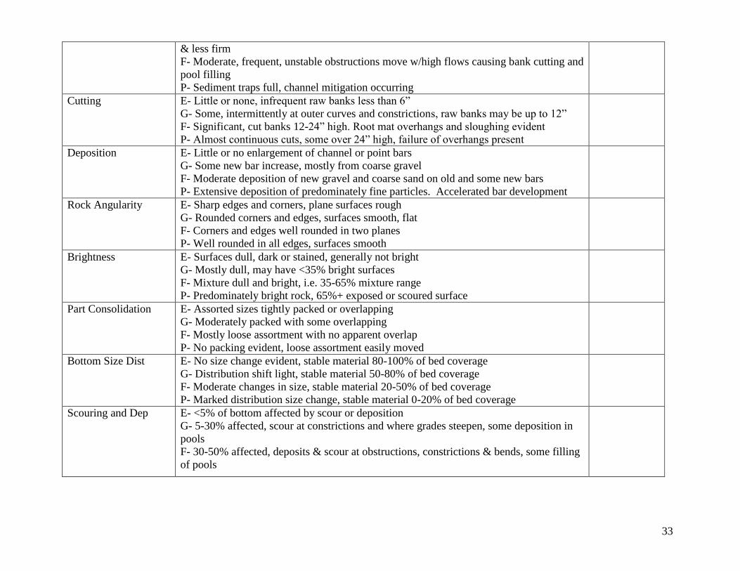
33
& less firm
F- Moderate, frequent, unstable obstructions move w/high flows causing bank cutting and
pool filling
P- Sediment traps full, channel mitigation occurring
Cutting E- Little or none, infrequent raw banks less than 6”
G- Some, intermittently at outer curves and constrictions, raw banks may be up to 12”
F- Significant, cut banks 12-24” high. Root mat overhangs and sloughing evident
P- Almost continuous cuts, some over 24” high, failure of overhangs present
Deposition E- Little or no enlargement of channel or point bars
G- Some new bar increase, mostly from coarse gravel
F- Moderate deposition of new gravel and coarse sand on old and some new bars
P- Extensive deposition of predominately fine particles. Accelerated bar development
Rock Angularity E- Sharp edges and corners, plane surfaces rough
G- Rounded corners and edges, surfaces smooth, flat
F- Corners and edges well rounded in two planes
P- Well rounded in all edges, surfaces smooth
Brightness E- Surfaces dull, dark or stained, generally not bright
G- Mostly dull, may have <35% bright surfaces
F- Mixture dull and bright, i.e. 35-65% mixture range
P- Predominately bright rock, 65%+ exposed or scoured surface
Part Consolidation E- Assorted sizes tightly packed or overlapping
G- Moderately packed with some overlapping
F- Mostly loose assortment with no apparent overlap
P- No packing evident, loose assortment easily moved
Bottom Size Dist E- No size change evident, stable material 80-100% of bed coverage
G- Distribution shift light, stable material 50-80% of bed coverage
F- Moderate changes in size, stable material 20-50% of bed coverage
P- Marked distribution size change, stable material 0-20% of bed coverage
Scouring and Dep E- <5% of bottom affected by scour or deposition
G- 5-30% affected, scour at constrictions and where grades steepen, some deposition in
pools
F- 30-50% affected, deposits & scour at obstructions, constrictions & bends, some filling
of pools
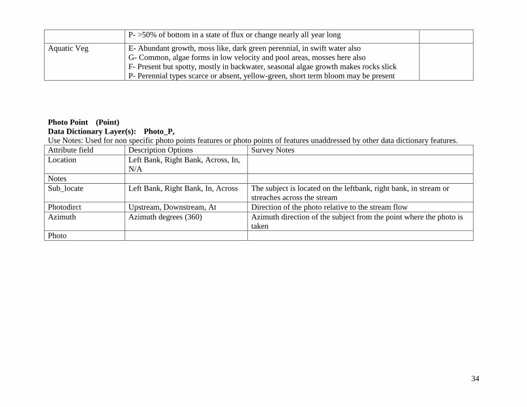
34
P- >50% of bottom in a state of flux or change nearly all year long
Aquatic Veg E- Abundant growth, moss like, dark green perennial, in swift water also
G- Common, algae forms in low velocity and pool areas, mosses here also
F- Present but spotty, mostly in backwater, seasonal algae growth makes rocks slick
P- Perennial types scarce or absent, yellow-green, short term bloom may be present
Photo Point (Point)
Data Dictionary Layer(s): Photo_P,
Use Notes: Used for non specific photo points features or photo points of features unaddressed by other data dictionary features.
Attribute field Description Options Survey Notes
Location Left Bank, Right Bank, Across, In,
N/A
Notes
Sub_locate Left Bank, Right Bank, In, Across The subject is located on the leftbank, right bank, in stream or
streaches across the stream
Photodirct Upstream, Downstream, At Direction of the photo relative to the stream flow
Azimuth Azimuth degrees (360) Azimuth direction of the subject from the point where the photo is
taken
Photo
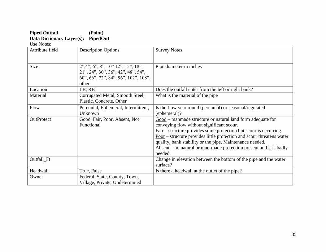
35
Piped Outfall (Point)
Data Dictionary Layer(s): PipedOut
Use Notes:
Attribute field Description Options Survey Notes
Size 2”,4”, 6”, 8”, 10” 12”, 15”, 18”,
21”, 24”, 30”, 36”, 42”, 48”, 54”,
60”, 66”, 72”, 84”, 96”, 102”, 108”,
other
Pipe diameter in inches
Location LB, RB Does the outfall enter from the left or right bank?
Material Corrugated Metal, Smooth Steel,
Plastic, Concrete, Other
What is the material of the pipe
Flow Perennial, Ephemeral, Intermittent,
Unknown
Is the flow year round (perennial) or seasonal/regulated
(ephemeral)?
OutProtect Good, Fair, Poor, Absent, Not
Functional
Good – manmade structure or natural land form adequate for
conveying flow without significant scour.
Fair – structure provides some protection but scour is occurring.
Poor – structure provides little protection and scour threatens water
quality, bank stability or the pipe. Maintenance needed.
Absent – no natural or man-made protection present and it is badly
needed.
Outfall_Ft Change in elevation between the bottom of the pipe and the water
surface?
Headwall True, False Is there a headwall at the outlet of the pipe?
Owner Federal, State, County, Town,
Village, Private, Undetermined
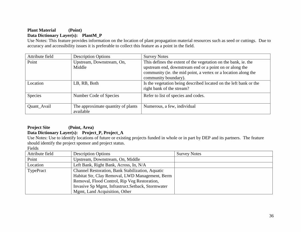
36
Plant Material (Point)
Data Dictionary Layer(s): PlantM_P
Use Notes: This feature provides information on the location of plant propagation material resources such as seed or cuttings. Due to
accuracy and accessibility issues it is preferable to collect this feature as a point in the field.
Attribute field Description Options Survey Notes
Point Upstream, Downstream, On,
Middle
This defines the extent of the vegetation on the bank, ie. the
upstream end, downstream end or a point on or along the
community (ie. the mid point, a vertex or a location along the
community boundary).
Location LB, RB, Both Is the vegetation being described located on the left bank or the
right bank of the stream?
Species Number Code of Species Refer to list of species and codes.
Quant_Avail The approximate quantity of plants
available
Numerous, a few, individual
Project Site (Point, Area)
Data Dictionary Layer(s): Project_P, Project_A
Use Notes: Use to identify locations of future or existing projects funded in whole or in part by DEP and its partners. The feature
should identify the project sponsor and project status.
Fields
Attribute field Description Options Survey Notes
Point Upstream, Downstream, On, Middle
Location Left Bank, Right Bank, Across, In, N/A
TypePract Channel Restoration, Bank Stabilization, Aquatic
Habitat Str, Clay Removal, LWD Management, Berm
Removal, Flood Control, Rip Veg Restoration,
Invasive Sp Mgmt, Infrastruct.Setback, Stormwater
Mgmt, Land Acquisition, Other
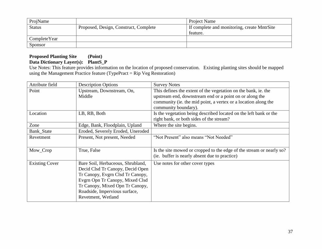
37
ProjName Project Name
Status Proposed, Design, Construct, Complete If complete and monitoring, create MntrSite
feature.
CompleteYear
Sponsor
Proposed Planting Site (Point)
Data Dictionary Layer(s): PlantS_P
Use Notes: This feature provides information on the location of proposed conservation. Existing planting sites should be mapped
using the Management Practice feature (TypePract = Rip Veg Restoration)
Attribute field Description Options Survey Notes
Point Upstream, Downstream, On,
Middle
This defines the extent of the vegetation on the bank, ie. the
upstream end, downstream end or a point on or along the
community (ie. the mid point, a vertex or a location along the
community boundary).
Location LB, RB, Both Is the vegetation being described located on the left bank or the
right bank, or both sides of the stream?
Zone Edge, Bank, Floodplain, Upland Where the site begins.
Bank_State Eroded, Severely Eroded, Uneroded
Revetment Present, Not present, Needed “Not Present” also means “Not Needed”
Mow_Crop True, False Is the site mowed or cropped to the edge of the stream or nearly so?
(ie. buffer is nearly absent due to practice)
Existing Cover Bare Soil, Herbaceous, Shrubland,
Decid Clsd Tr Canopy, Decid Open
Tr Canopy, Evgrn Clsd Tr Canopy,
Evgrn Opn Tr Canopy, Mixed Clsd
Tr Canopy, Mixed Opn Tr Canopy,
Roadside, Impervious surface,
Revetment, Wetland
Use notes for other cover types
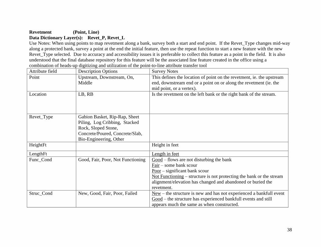
38
Revetment (Point, Line)
Data Dictionary Layer(s): Revet_P, Revet_L
Use Notes: When using points to map revetment along a bank, survey both a start and end point. If the Revet_Type changes mid-way
along a protected bank, survey a point at the end the initial feature, then use the repeat function to start a new feature with the new
Revet_Type selected. Due to accuracy and accessibility issues it is preferable to collect this feature as a point in the field. It is also
understood that the final database repository for this feature will be the associated line feature created in the office using a
combination of heads-up digitizing and utilization of the point-to-line attribute transfer tool
Attribute field Description Options Survey Notes
Point Upstream, Downstream, On,
Middle
This defines the location of point on the revetment, ie. the upstream
end, downstream end or a point on or along the revetment (ie. the
mid point, or a vertex).
Location LB, RB Is the revetment on the left bank or the right bank of the stream.
Revet_Type Gabion Basket, Rip-Rap, Sheet
Piling, Log Cribbing, Stacked
Rock, Sloped Stone,
Concrete/Poured, Concrete/Slab,
Bio-Engineering, Other
HeightFt Height in feet
LengthFt Length in feet
Func_Cond Good, Fair, Poor, Not Functioning Good – flows are not disturbing the bank
Fair – some bank scour
Poor – significant bank scour
Not Functioning – structure is not protecting the bank or the stream
alignment/elevation has changed and abandoned or buried the
revetment.
Struc_Cond New, Good, Fair, Poor, Failed New – the structure is new and has not experienced a bankfull event
Good – the structure has experienced bankfull events and still
appears much the same as when constructed.
39
Fair – the structure has deteriorated and may be missing stones, may
have gaps, settled or rotated materials, failed support plantings, may
show evidence of the scour or aggradation.
Poor – the structure is crumbling, slumping, covered with sediment,
scoured out, show evidence of the significant likelihood that failure
can be expected in the near future.
Failed – the structure has been significantly damaged. Ie. it has
been washed away, buried, or no longer protects the bank.
BankKeyed True, False, Unknown Is the revetment tied back into the bank?
ScourProt True, False, Unknown Is the toe protected from scour?
Road (Point, Line)
Data Dictionary Layer(s): Road_P, Road_L
Use Notes: This feature should be captured where a road or trail either crosses the stream or may impact the stream and its floodplain.
Due to accuracy and accessibility issues it is preferable to collect this feature as a point in the field. It is also understood that the final
database repository for this feature will be the associated line feature created in the office using a combination of heads-up digitizing
and utilization of the point-to-line attribute transfer tool
Attribute Fields Description options Survey Notes
Location Left bank, Right bank
Position Centerline, Edge, Ditch, Guiderail Feature of the road that is being captured
Material Paved, Gravel, Vegetation, Dirt,
Other
Road_Use Auto, RR, Trail, Recreation
Vehicles, Ag Use, Forestry, Other
Principle use
Owner State, County, Town, Private,
Federal, Undetermined
Road_Name Fill in the name
40
Road Glossary:
RR – working or abandoned railroad right of way – not including a rail trail. For rail trail see trail.
Trail – a path or improved route including a rail trail typically not used by motorized recreational vehicles
Recreational vehicle – trails used by recreational vehicles…atvs, snowmobiles, etc.
Ag. Use – farm road or tracks traveled by heavy equipment
Forestry – logging trails or roads including those that have not been used recently
Rosgen Level 1 Classification (Point)
Data Dictionary Layer(s): RosgenL1
Use Notes: This feature is captured in the field when the surveyor encounters what is believed to be a change in the Rosgen
Classification Stream Type. The point should be taken in the thalweg, preferably at a feature break. This can be used to verify
office based classification or add additional breaks at the time of a walkover.
Attribute Fields Description options Survey Notes
ClassAbove Aa+-G,Undetermined What is the likely classification of the upstream reach?
ClassBelow Aa-G,Undetermined What is the likely classification of the reach below this point?
Reference True,False Is this possibly a reference reach (at first glance, does it have
indicators that suggest it might be stable?)
Rosgen Level 1 Class Glossary:
Sediment Sample Location (Point)
Data Dictionary Layer(s): SedSample
Use Notes: This feature is captured at the location of sediment samples such as a bar sample or pebble count
Attribute Fields Description options Survey Notes
Samp_Type Bulk, Pebble
Sample_Locat Bed, Bar, Bank, Other
Number Id number
D84_Est This is estimated
D50_Est This is estimated
41
Site Visit (Point)
Data Dictionary Layer(s): Visit_P
Use Notes: This feature is captured at the time of a site visit.
Attribute Fields Description options Survey Notes
Program Name of program responsible for the site visit i.e. SAP, CWC,
EWP…
DateVisit Date of visit
TypePract Channel Restoration, Bank
Stabilization, Aquatic Habitat Str,
Clay Removal, LWD Management,
Berm Removal, Flood Control, Rip
Veg Restoration, Invasive Sp
Mgmt, Infrastruct Setback,
Stormwater Mgmt, Land
Acquisition, Other
OwnerName Name of the land owner or local sponsor.
Sponsor Sponsoring agency or group.
Estimated cost
Visited By Name
42
Stream Feature (Point, Line)
Data Dictionary Layer(s): SFeat_P, SFeat_L
Use Notes: This feature can be used to create stream alignments and define the breaks in features along the stream. The point should
be taken in the thalweg, preferably at a feature break. Due to accuracy and accessibility issues it is preferable to collect this
feature as a point in the field. It is also understood that the final database repository for this feature will be the associated line feature
created in the office using a combination of heads-up digitizing and utilization of the point-to-line attribute transfer tool
Attribute field Description Options Survey Notes
Point Upstream, Downstream, On,
Middle
This defines the location of point on the stream feature, ie. the
upstream start, downstream end or a point on or along the stream
feature (ie. the mid point, or a vertex).
Location Thalweg, Right, Left, On Center
Bar
Is the location where the point is being taken. Normally this should
be “Thalweg”, but in the case of a divergence or convergence it
might “On Center Bar”.
Feat_Type Riffle, Run, Pool, Glide, Step, Step
Pool Sequence, Scour, Headcut,
Cascade, Divergence,
Convergence, Other
Taken at the top of the feature. See Stream Feature Glossary
Reference True, False Could this be a reference reach? This is only to indicate where a
future reference reach survey might be undertaken.
Channel Main, Secondary, Other Is the point you are taking located on the main channel or a
secondary channel?
SC_Type Flood Chute, Avulsion, Backwater
Area, Other, Side Channel
Secondary Channel Type. This attribute is used in combination with
the Channel attribute. It provides more detail about the type of
secondary channel.
Change_Ft Elevation change between the top and bottom of a feature.
Especially used for headcut
LengthFt Required only if using middle under location
Flow Perennial, Intermittent, Subsurface,
Unknown
Is the channel flowing? Can be used to capture areas of subsurface
flow
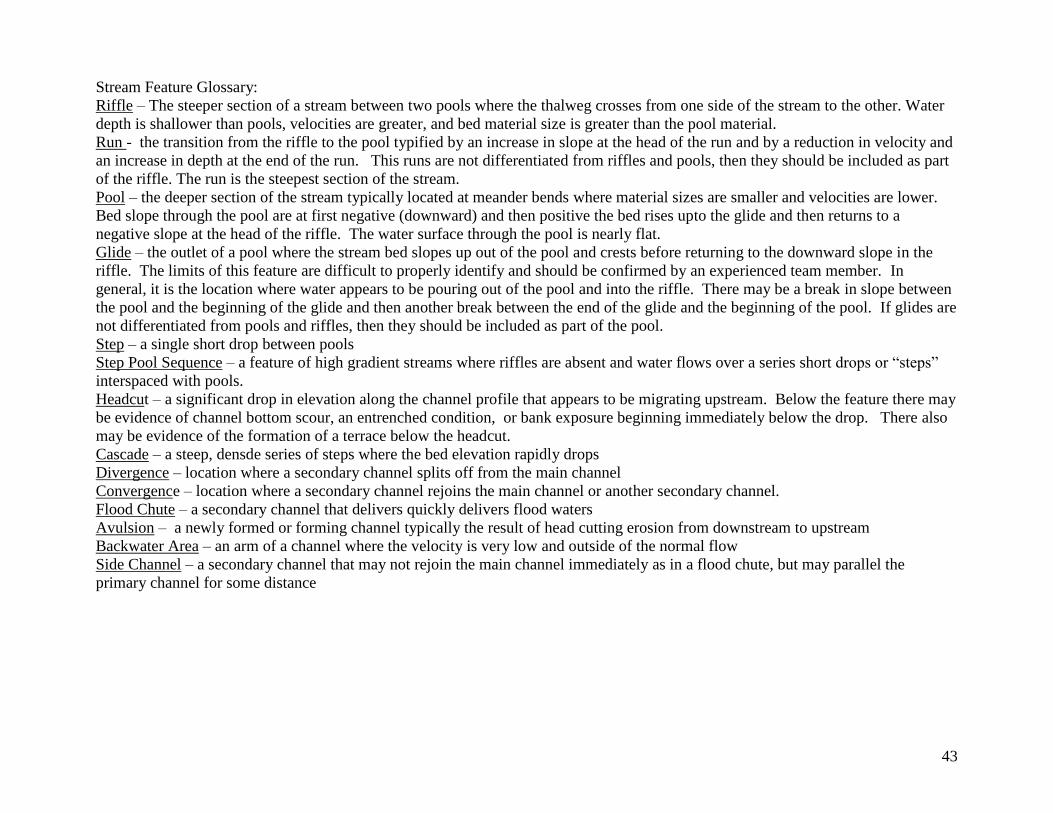
43
Stream Feature Glossary:
Riffle – The steeper section of a stream between two pools where the thalweg crosses from one side of the stream to the other. Water
depth is shallower than pools, velocities are greater, and bed material size is greater than the pool material.
Run - the transition from the riffle to the pool typified by an increase in slope at the head of the run and by a reduction in velocity and
an increase in depth at the end of the run. This runs are not differentiated from riffles and pools, then they should be included as part
of the riffle. The run is the steepest section of the stream.
Pool – the deeper section of the stream typically located at meander bends where material sizes are smaller and velocities are lower.
Bed slope through the pool are at first negative (downward) and then positive the bed rises upto the glide and then returns to a
negative slope at the head of the riffle. The water surface through the pool is nearly flat.
Glide – the outlet of a pool where the stream bed slopes up out of the pool and crests before returning to the downward slope in the
riffle. The limits of this feature are difficult to properly identify and should be confirmed by an experienced team member. In
general, it is the location where water appears to be pouring out of the pool and into the riffle. There may be a break in slope between
the pool and the beginning of the glide and then another break between the end of the glide and the beginning of the pool. If glides are
not differentiated from pools and riffles, then they should be included as part of the pool.
Step – a single short drop between pools
Step Pool Sequence – a feature of high gradient streams where riffles are absent and water flows over a series short drops or “steps”
interspaced with pools.
Headcut – a significant drop in elevation along the channel profile that appears to be migrating upstream. Below the feature there may
be evidence of channel bottom scour, an entrenched condition, or bank exposure beginning immediately below the drop. There also
may be evidence of the formation of a terrace below the headcut.
Cascade – a steep, densde series of steps where the bed elevation rapidly drops
Divergence – location where a secondary channel splits off from the main channel
Convergence – location where a secondary channel rejoins the main channel or another secondary channel.
Flood Chute – a secondary channel that delivers quickly delivers flood waters
Avulsion – a newly formed or forming channel typically the result of head cutting erosion from downstream to upstream
Backwater Area – an arm of a channel where the velocity is very low and outside of the normal flow
Side Channel – a secondary channel that may not rejoin the main channel immediately as in a flood chute, but may parallel the
primary channel for some distance
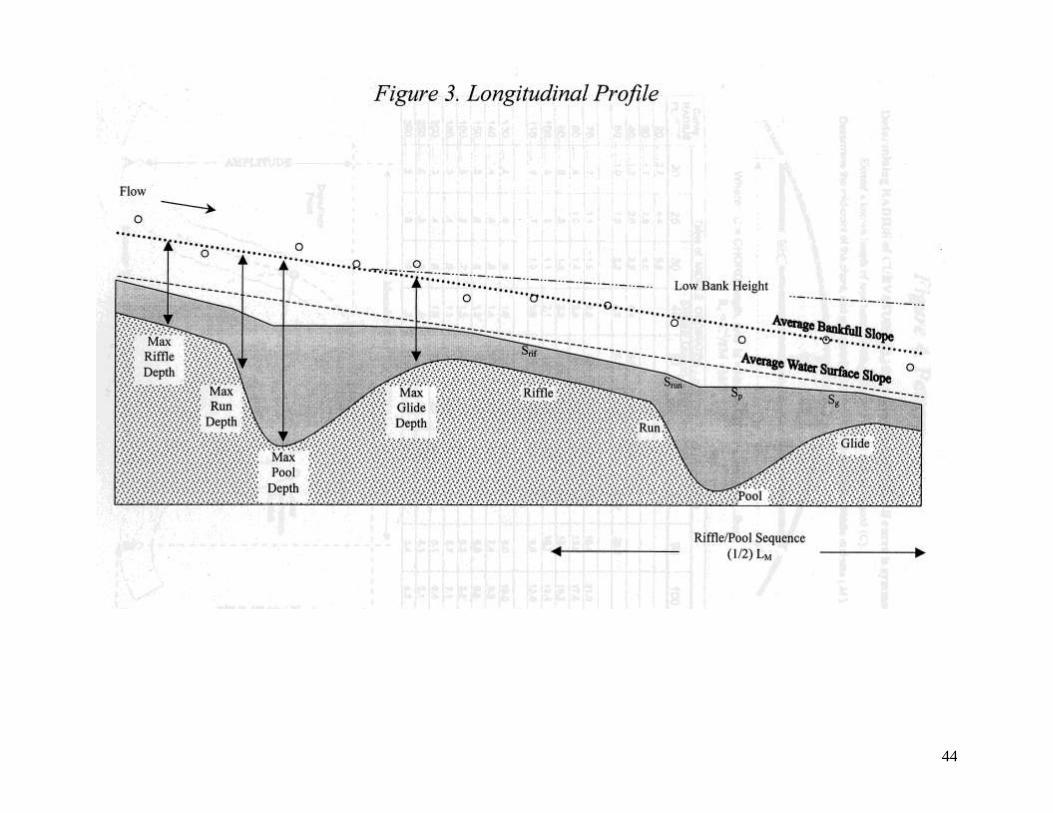
44
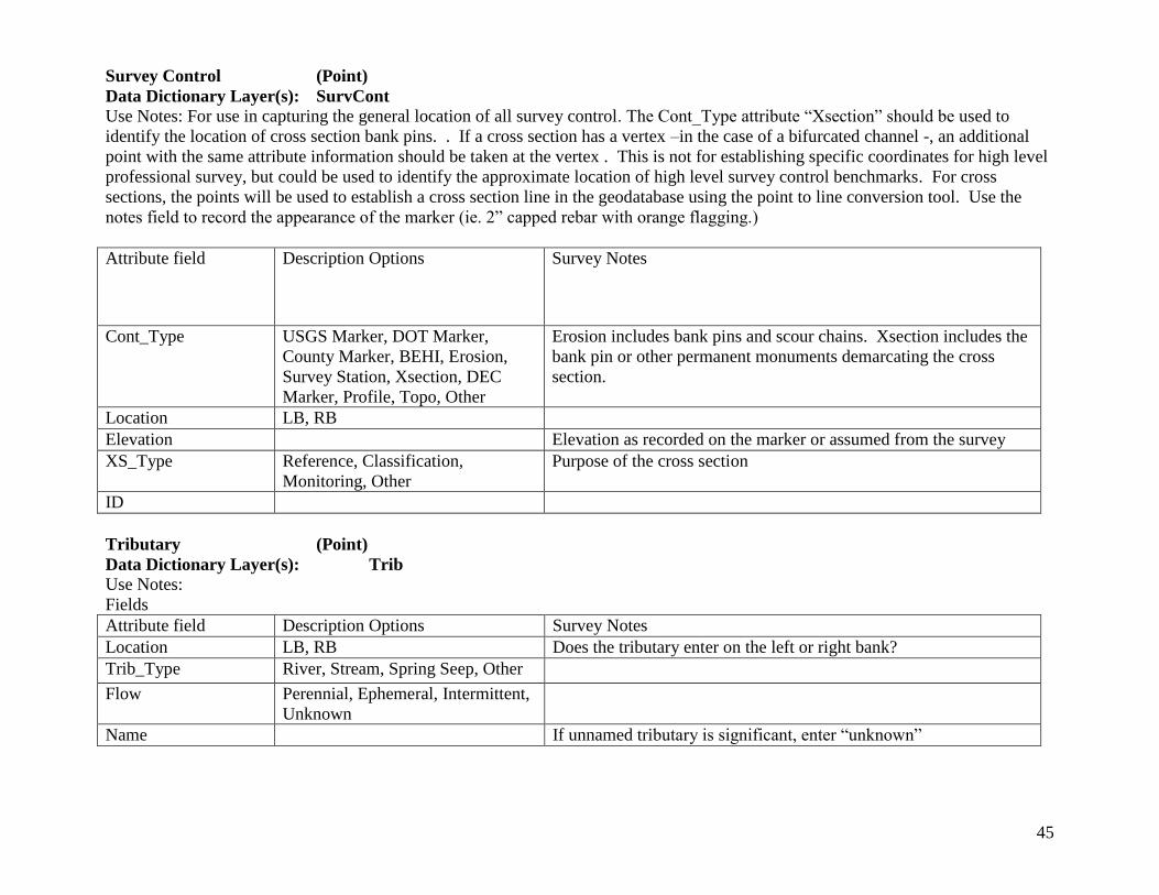
45
Survey Control (Point)
Data Dictionary Layer(s): SurvCont
Use Notes: For use in capturing the general location of all survey control. The Cont_Type attribute “Xsection” should be used to
identify the location of cross section bank pins. . If a cross section has a vertex –in the case of a bifurcated channel -, an additional
point with the same attribute information should be taken at the vertex . This is not for establishing specific coordinates for high level
professional survey, but could be used to identify the approximate location of high level survey control benchmarks. For cross
sections, the points will be used to establish a cross section line in the geodatabase using the point to line conversion tool. Use the
notes field to record the appearance of the marker (ie. 2” capped rebar with orange flagging.)
Attribute field Description Options Survey Notes
Cont_Type USGS Marker, DOT Marker,
County Marker, BEHI, Erosion,
Survey Station, Xsection, DEC
Marker, Profile, Topo, Other
Erosion includes bank pins and scour chains. Xsection includes the
bank pin or other permanent monuments demarcating the cross
section.
Location LB, RB
Elevation Elevation as recorded on the marker or assumed from the survey
XS_Type Reference, Classification,
Monitoring, Other
Purpose of the cross section
ID
Tributary (Point)
Data Dictionary Layer(s): Trib
Use Notes:
Fields
Attribute field Description Options Survey Notes
Location LB, RB Does the tributary enter on the left or right bank?
Trib_Type River, Stream, Spring Seep, Other
Flow Perennial, Ephemeral, Intermittent,
Unknown
Name If unnamed tributary is significant, enter “unknown”

46
Utility (Point)
Data Dictionary Layer(s): Utility
Use Notes:
Attribute field Description Options Survey Notes
Util_Type Pole, Well, Phone, Sewer, Water,
Cable, Gas, Hydrant, Multiple
Util_ID If the pole has a id number
Owner Public, Private, Unknown
Orient Parallel, Perpendicular Does the utility line run approximately parallel or across
(perpendicular to the stream
Utility Glossary:
47
Subject Index
Bar ................................................................. Depositional Feature, Dep_Feat, 20
Erosion Types ................................................................... Bank Erosion, Bank_P, Bank_L, 7
Fascine ............................................ Best Management Practice, BMP_P, BMP_L, 14
Grade control ................................................................... Control, Control_P, Control_L, 17
Undercut Bank ................................................................... Bank erosion, Bank_P, Bank L, 7
Vane ............................................ Best Management Practice, BMP_P, BMP_L, 14

Attachment B:
Fluvial Geomorphology Survey Field Forms and Checklists
DEP, July 31, 2017

FG Survey Data Sheet 1 Revision: 07/14/2017 Page __ of __
Fluvial Geomorphology Survey: Longitudinal ProfileWatershed/Stream: Date:Site ID: Team Member/TaskStation Start: Station End:Equipment:Weather (current/previous): Data Processed in RMP/Excel?Bench Mark/Elev: GPS Recorded?Further information in Field Book/Page#/ Calculation Sheets #/Date:All measurements in feet
Station BS (+) HI FS (-) Elev Description Comments
Survey Point Legend
Closure Error: LEW - Left edge water REW - Right edge waterTime Start: LBF - Left bankfull RBF - Right bankfullTime End: TH - Thalweg WS - Water surface (ft)
RTOB - Right top of bank LTOB - Left top of bankHI = BS + previous Elev Elev = HI - FS HWM - High water mark (L/R) WD - Water depth (ft)DO NOT erase recorded data; errors are shown with TOR - top of riffle BOR - bottom of rifflea single horizontal line through the rcorded number. TOS - top of step BOS - bottom of step
Data Validation: _________________________ TOP - top of pool BOP - bottom of poolBM - Bench mark
Data Verification: ______________________

FG Survey Data Sheet 2 Revision: 07/14/2017 Page __ of __
Fluvial Geomorphology Survey: Channel Cross SectionWatershed/Stream: Date: LP Date:Site ID: Team Member/TaskXS ID: Pool/Glide/Riffle/Run/StepEquipment: LP station: Slope:Weather (current/previous): Data Processed in RMP/Excel?Time (start/finish): GPS Recorded?Further information in Field Book/Page# or Calculation Sheets:BM Description: BM Elev: BS (+) Height of Instrument:All measurements in feet
Station FS (-) Elev Code Description Station FS (-) Elev Code Description
Closure Error: PHOTOS: Camera#: Survey Point Legend:Stage/Time Start: US-DS: LPIN - Left pin RPIN - Right pinStage/Time End: DS-US: LTOB - Left top bank RTOB - Right top bankData Validation: L-R: LBF - Left bankfull RBF - Right bankfullData Verification: R-L: LEW - Left edge water REW - Right edge water
LPIN: TH - Thalweg BTM - Channel BottomRPIN: TP - Turning Point HWM - High Water MarkBKF: GR - Ground FP - Floodplain
HI= BS + Previous Elev Elev= HIS-FSDO NOT erase recorded data; errors are shown witha single horizontal line through the rcorded number.
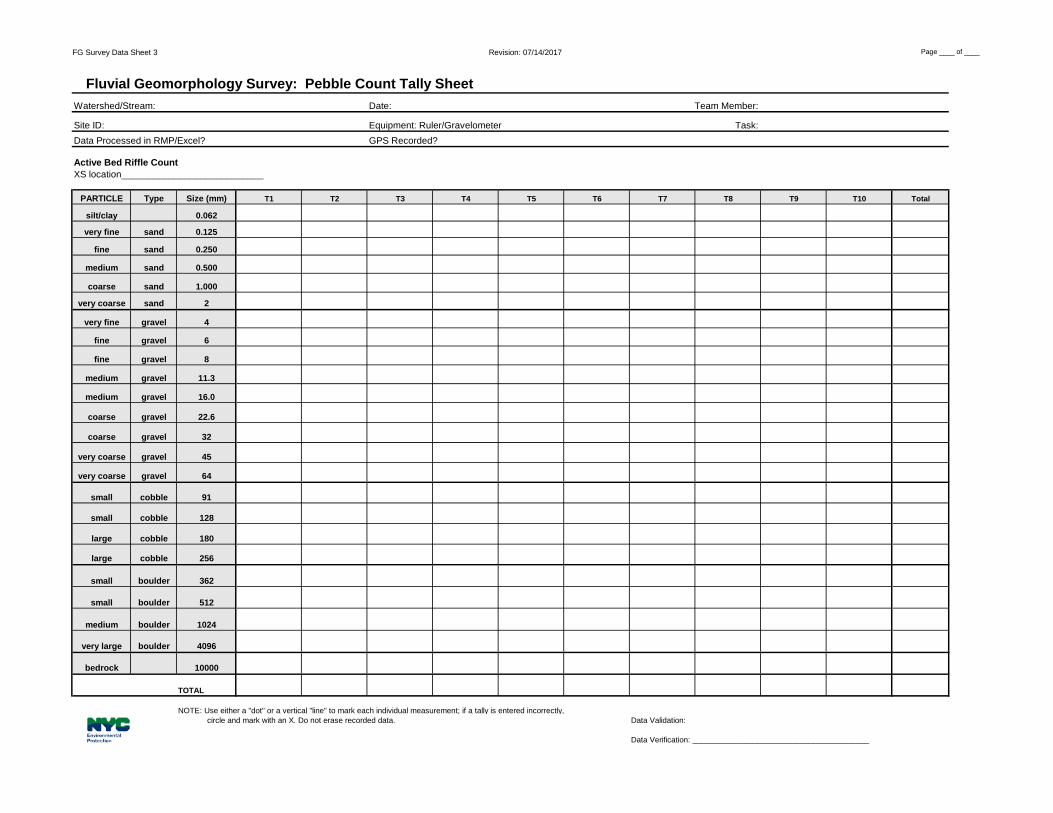
FG Survey Data Sheet 3 Revision: 07/14/2017 Page ____ of ____
Fluvial Geomorphology Survey: Pebble Count Tally SheetWatershed/Stream: Date: Team Member:
Site ID: Equipment: Ruler/Gravelometer Task:Data Processed in RMP/Excel? GPS Recorded?
Active Bed Riffle CountXS location___________________________
PARTICLE Type Size (mm) T1 T2 T3 T4 T5 T6 T7 T8 T9 T10 Total
silt/clay 0.062
very fine sand 0.125
fine sand 0.250
medium sand 0.500
coarse sand 1.000
very coarse sand 2
very fine gravel 4
fine gravel 6
fine gravel 8
medium gravel 11.3
medium gravel 16.0
coarse gravel 22.6
coarse gravel 32
very coarse gravel 45
very coarse gravel 64
small cobble 91
small cobble 128
large cobble 180
large cobble 256
small boulder 362
small boulder 512
medium boulder 1024
very large boulder 4096
bedrock 10000
TOTAL
NOTE: Use either a "dot" or a vertical "line" to mark each individual measurement; if a tally is entered incorrectly, circle and mark with an X. Do not erase recorded data. Data Validation: __________________________________________
Data Verification: _________________________________________
FG Survey Sheet 4 Revision: 07/14/2017 Page ____ of ____
Fluvial Geomorphology Survey: Pebble Count Tally SheetWatershed/Stream: Date: Team Member:
Site ID: Equipment: Ruler/Gravelometer Task:Data Processed in RMP/Excel? GPS Recorded?Representative Reach Pebble Count Label each transect with the feature sampled: Riffle/Pool/Setp/Run/Plane Bed
STN:Feature:
PARTICLE Type Size (mm) T1 T2 T3 T4 T5 T6 T7 T8 T9 T10 Total
silt/clay 0.062
very fine sand 0.125
fine sand 0.250
medium sand 0.500
coarse sand 1.000
very coarse sand 2
very fine gravel 4
fine gravel 6
fine gravel 8
medium gravel 11.3
medium gravel 16.0
coarse gravel 22.6
coarse gravel 32
very coarse gravel 45
very coarse gravel 64
small cobble 91
small cobble 128
large cobble 180
large cobble 256
small boulder 362
small boulder 512
medium boulder 1024
very large boulder 4096
bedrock 10000
TOTAL
NOTE: Use either a "dot" or a vertical "line" to mark each individual measurement; if a tally is entered incorrectly, circle and mark with an X. Do not erase recorded data. Data Validation: __________________________________________
Data Verification: _________________________________________

FG Survey: Data Sheet 5 Revision: 07/14/2017 Page __ of __
Fluvial Geomorphology Survey: CalculationsWatershed/Stream: Date:Reach ID: Calcs By:Further information in Field Book/Page# or Data Sheets:
Data Validation: __________________________________
Data Verification: ___________________________________

FG Survey Data QA/QC Sheet 1 Revision 07/14/2017 Page __ of __
FLUVIAL GEOMORPHOLOGY SURVEYS: LONGITUDINAL PROFILE CHECKLIST
CHECKED BY: DATE: LP ID:
PROJECT ID:
1. All items filled out in header:Watershed/Stream Date Field Book/Calc Sheet ReferencedSite ID BM ID/ElevStation Start Team Member/TaskStation End Data ProcessedWeather GPS RecordedEquipment Page #
2. Set HI and Check HI calculated, error identified and clearly noted on Data Sheet or Calculation Sheet
3. All Station, BS, HI, FS, Elevation, Description and Comment cells are filled out and legible, or have a strikethrough line if left intentionally blank.
4. LP Survey time start/end noted
5. If present L/R BKF is noted, with description of feature and any info on pin flag included in comments column.
6. If present, cross-section stations are recorded and noted in Comments column.
7. NOTES for next level of review
PROJECT LEADER VALIDATION: _______________________________________
NOTES:
FG Survey QA/QC Sheet 2 Revision: 07/14/2017 Page __ of __
FLUVIAL GEOMORPHOLOGY SURVEYS: CROSS SECTION CHECKLIST
CHECKED BY: DATE: XS ID:
PROJECT ID:
1. All items filled out in header:Watershed/Stream Date Data ProcessedSite ID LP Date GPS RecordedXS ID Team Member/Task Page #Feature selected LP Station Field Book/Calc Sheet ReferencedWeather LP SlopeTime S/F
2. All items filled out for Establishing Height of Instrument:BM Identified BM Elev BS HI
3. All Station, FS, Elevation, Code and Description cells are filled out and legible, or have a strikethrough line if left intentionally blank.
4. Photos taken and noted on data sheet. Was a white board used to identify XS?Upstream looking downstreamDownstream looking upstreamLeft to right bankRight to left bankLPINRPINFlagged BKF
5. Monument pin locations in cross section noted, including the top of pin shot and if necessary, a ground shot next to the pin.
6. L/R BKF is noted, with description of feature in notes column. Alternative BKF features noted?
7. NOTES for next level of review
PROJECT LEADER VALIDATION: _______________________________________
NOTES:

FG Survey QA/QC Sheet 3 Revision: 07/14/2017 Page __ of __
FLUVIAL GEOMORPHOLOGY SURVEYS: PEBBLE COUNT TALLY SHEET CHECKLIST
CHECKED BY: DATE: LP/XS ID:
PROJECT ID:
1. All items filled out in header:Watershed/Stream Team Member/TaskSite ID Data ProcessedDate GPS RecordedEquipment Page #
2. If Active Bed Riffle Count Sheet is XS location provided?
3. If Representative Reach Pebble Count Sheet are the stations and bedform features labeled?
4. Are all tally marks (dots or lines) legible and any errors noted with a circled X?
5. Do all columns total at least 10 points per transect?
6. Are all tally totals summed per particle size category?
7. Are all tally totals summed with a total of at least 100 counts?
8. NOTES for next level of review
PROJECT LEADER VALIDATION: _______________________________________
NOTES:

Appendix C:
AWSMP SOP#2: Project Monitoring.
Ashokan Watershed Stream Management Program, February, 2016

AWSMP SOP #2: Project Monitoring
AWSMP SOP #2: Project Monitoring Objectives
o Meet US Army Corps of Engineers (ACOE) permit requirements o Evaluate project success o Determine any corrective or maintenance requirements o Learn how to improve techniques for future projects
Needed Equipment o Survey equipment (preferably total station) o Two or more full length 300-ft survey tapes o Two or more clamps o GPS with appropriate files (monument and photo monitoring locations) o Camera o Rebar & rebar caps o Steel hammer o Compass o Flagging pins and flagging tape o 2-way handheld radios o Field forms & maps o Loppers/Machete o Project monitoring binder with useful information o Field form types: station setup and benchmark log, XS, longitudinal profile, and pebble count. It
is also good to include something to record general notes of photo monitoring, wildlife observations, monument tie-ins (consider blank sheets for sketches or leaving back sides blank), and anything else that may come up.
Establishing New Project Monitoring Sites 1) Establish Monitoring Objectives and Project Success Criteria
o AWSMP partners will collaborate to identify the key monitoring objectives for each project site during the fall or winter following construction completion.
o Determine project success criteria which will guide monitoring and data collection. The success criteria provides a quantity to compare to monitoring data for evaluating the effectiveness of the project installation in addressing the original goals/purpose of the project as well as performance of specific design elements/structures.
2) Project Monitoring Layout a. Create Monitoring Instructions that outlines the requirements for the specific project
site. This includes the location, if there is an ACOE permit and which years are required to be monitored, tasks, instructions, and background information. See other project’s instructions for examples. Save the document here: W:\Streams\Monitoring\Project Monitoring\[stream name]\Documents\Monitoring Protocol and XS Info\[project name].
1

AWSMP SOP #2: Project Monitoring
b. Review the As-Built planform map and pre-determined site-specific objectives to determine where cross sections (XS) should be installed. This can be done in the office but being on site may be beneficial. Mark up the map where XSs should be installed along with any key details and if on site, leave flagging pins on one bank to mark general locations.
Cross Section Site Selection Criteria
• Riffle for Rosgen’s stream classification (ACOE report requirement) • Structure performance • Hillslope adjustment • Channel response • Habitat • Uninfluenced areas outside of the project site for comparison to constructed
features
Generally XSs through pools and vane structures are lined up to go through the deepest part of the pool while also avoiding the sills of vane structures. Similarly avoid the line of boulders for constructed steps (riffles), although they tend to have curvature that makes it impossible to avoid completely. XSs selected for sheet piling should be installed below the sheet piling to capture scour.
c. Verify that there is a benchmark (BM) with known elevation prior to beginning data collection. This will serve as the initial occupy point of the total station. Make sure to write detailed notes when setting up the data logger/total station “job” during data collection. These notes need to be detailed enough to be replicated in future years. At minimal record the following: Coordinate system (likely local), what BM is the occupy point, the BM’s coordinates (generally use N = 10,000 ft and E = 5,000 ft rather than true coordinates), the BM’s reported elevation (likely from the As-Built unless it is a FEMA-NYCDEP monument), what backsight was used, and the inputted compass bearing to the BS. Include a detailed description of the BS if it is not a typical rebar monument.
2) Monumenting Cross Sections and Benchmarks a. Ensure XSs are perpendicular to flow by running a 300-ft tape across the channel and
using the line as a guide. b. Use 2-ft or longer rebar for both XS monuments and benchmarks. Drive the rebar low to
the ground, especially in areas that are accessed by people. c. Place caps and flagging tape on the monuments. Also flag a nearby tree. d. XSs may have more than two monuments if a 300-ft tape is not long enough to capture
the desired area (ex: hillslopes) or there is an interest to capture the wide floodplains but not necessarily to resurvey the entire length each time.
e. Occasionally a XS can be set up without using a permanent rebar monument, such as using the corner of a shed or a deck railing. This is desirable when the XS coincides with the landowner’s lawn or heavily used areas. Make sure to take detailed notes of the “ending pin” to ensure reproducibility and a photo with the prism pole being held at the “ending pin.”
2
AWSMP SOP #2: Project Monitoring
f. Naming convention: The upstream cross section should be called XS-01. If there are multiple project sites that will be recorded within the same survey “job” file, then do not restart the numbering for each site. For example: Chichester Site 2-3 begins with XS-06 since Chichester Site 1 ended with XS-05.
g. Important: Detailed documentation of monument locations i. Take photos of the monuments and any notes that will assist in locating the
monuments in future years. Photos from a distance with a person standing at the monument is more useful then close up photos. Try to capture something to provide reference relative to the monuments (trees, fences, structures, immobile boulders, etc.).
ii. Record location (GPS) of each monument (XSs and benchmarks). iii. Record the compass bearing for each XS from one monument to the other and
specify the direction (ex: LEP to REP). Use the XS tape as a guide or have someone stand at the opposite monument.
3) Data Collection – Methods for conducting cross sections, longitudinal profiles, pebble counts and using survey equipment should follow the procedures outlined in these protocols:
• General Stream Survey Techniques o SOP #4 - General Stream Survey Techniques o USFS Stream Channel Reference Sites: Illustrated Guide to Field
Technique (Harrelson et al., 1994) o River Stability Field Guide – Level II Assessment (Rosgen, 2008)
• SOP #5 – Trimble Geo7X Series • SOP #6 – Using the Robotic Total Station
The following is a summary of field tasks to be completed for each project monitoring site.
a. Cross Sections – Survey each XS and take photos while the tape is still up. Verify that the XS is wide enough to capture the full flood prone width by doing the following:
i. Determine maximum depth (the elevational difference between bankfull and thalweg).
ii. Double maximum depth and add this to the thalweg elevation. iii. Check that this elevation is reached on both the RB and LB. If not, extend the
XS beyond the ending pin until this elevation is achieved. Make note if this was required so that it can be added to the site specific monitoring instructions.
b. Photo Monitoring Points – These can be set up in advance or established during data collection. Record location (GPS) of each photo point as well as which photo numbers go to each point. Choose locations that have long, unobstructed line of sight to minimize the number of points required to cover the entire project area. The locations should also be easily accessible during high flow events, such as being out of the channel and along the roadside bank. Choose enough locations to span the entire project area, capture the downstream and upstream reaches, and areas of disturbed riparian forest.
c. Longitudinal Profile – Survey the longitudinal profile. Profile must include entire length of the project and should start and end at the top of a riffle. Document the starting location so that it can be reproduced each year. Ensure points are recorded at each of
3
AWSMP SOP #2: Project Monitoring
the cross sections. Noting the location of the cross sections on the longitudinal profile will allow for better comparison between profile surveys. If the project site involves a confluence, survey both stream channels.
d. Pebble Count – For channel classification and ACOE permit requirements, a representative pebble count is needed. Use the AWSMP Pebble Count Form to record data and follow the instructions outlined in the Level II Assessment – Representative Pebble Count in the River Stability Field Guide (Rosgen, 2008).
e. Local Topo – For some structures, it is beneficial to record topography in an area rather than just a straight line. Local topo’s should be done for specific features in which an area is needing to be evaluated (e.g. track where sediment is accumulating around a structure and where scour is occurring).
f. Vegetation – Some ACOE permits require ensuring 85% survival and/or coverage rate by the end of the second growing season on bank stabilization sites. If available, Catskill Streams Buffer Initiative (CSBI) vegetation monitoring results can be used.
g. Wildlife – Some sites require documenting wildlife observations for ACOE permit requirements. Check the permit specific to the site. If required, make notes of any wildlife observed and the general location, ex: heron resting on Site 2 hillslope.
h. Additional – Consider any objectives specific to the project site that require unique procedures. For example: A few points along the 50-year wall at Stony Clove Lane were marked and surveyed to monitor any shifting of the wall. Any unique procedures should also be added to the site specific monitoring instructions.
Frequency of Monitoring 1) ACOE Permit Requirements –
o The first two field seasons after the project is completed to meet the ACOE permit requirements. Reports must be submitted no later than October 31st.
o Bankfull events – Photo documentation is needed of the annual high flow event for inclusion in reports (preferably peak). In the event this occurs, staff will need to visit project sites that still require ACOE reports and photo document site conditions.
2) AWSMP Objectives – o Beginning with the third year, monitoring efforts will be continued according to AWSMP
goals and objectives. o Frequency of surveys will depend on the projects objectives. In general, after the first
two years following project construction and ACOE monitoring requirement have been completed, frequency of monitoring will depend on the occurrence of geomorphically significant flood events (e.g. bankfull or greater magnitude). In addition, it may be determined that only a subset of the original tasks need repeating.
o Bankfull events – At a minimum, project sites should be visited during or directly after peak-flow to photo document the project’s performance during flood stage and record extents of inundation. Pin flags should be placed at high water marks (to be surveyed later), especially at project sites that have not experienced a bankfull event since construction.
Revisiting Established Project Monitoring Sites
4
AWSMP SOP #2: Project Monitoring
1) Locate, resurvey, and take photos of the cross sections. a. The monitoring map combined with nearby flagged trees may be good enough to locate
the XS monuments. If not, use the GPS to navigate and/or use notes & the printed photos in the monitoring binder.
b. If a particular XS has more than two monuments, survey the inner (streamside) monuments unless a streamflow event occurred that gained access beyond the inner monuments, in which case the entire XS should be surveyed.
c. Take photos with the XS tape up. 2) Resurvey any local topos if a bankfull or larger flow event occurred. 3) Take photos at the photo monitoring points by using the GPS to navigate to the locations.
Record in field notes which photos go to which point. 4) Resurvey the longitudinal profile. Be sure to record points where cross sections intersect the
profile. 5) Complete a representative pebble count for the second monitoring year (ACOE requirement)
and thereafter as is deemed necessary for AWSMP objectives. 6) Complete any tasks specific to the site, such as monitoring the 50-year wall at Stony Clove Lane
mentioned in the above section. Keep in mind that some sites require documenting wildlife observations for ACOE permit requirements.
Important Surveying Practices • Data density/detail – In general, it is important to stay consistent with the level of detail
collected from survey to survey. Review previous surveys for a monitoring site to know how densely data should be recorded in cross sections and longitudinal profiles. The goal is to record enough points to accurately reflect the general shape while balancing between too much and too little data. Collecting too much data makes it difficult to compare data between years, as well as being time consuming; while collecting too little data does not accurately reflect the XS by oversimplifying. Harrelson et al. (1994) recommends collecting at least 20 measurements for most channels to accurately depict them. Exceptions are complex or broad locations, such as braided channels or trying to capture complex failures on hillslopes. A sample of 2015 project monitoring XSs ranged from 18 to 38 points over a wide range of XS length and complexity. Bringing print-outs of the previous survey graphs may be beneficial in determining the amount of detail to record.
• Whenever a point is foresighted to be a station or temporary benchmark, make sure to mark the location on the monitoring map and label its code (S1, TBM2, etc.). It is also useful to write the date when the point was first measured, such as est. 7/1 for established. This combined with the station setup log can be useful when trying to correct mistakes. The labeled monitoring map is also useful when trying to recall point names when returning on later days, with different crew members, or when there are numerous occupy points. It may also be useful to use a sharpie to write the point number, code, and year on the flagging tape around the temporary benchmarks; the year will help prevent confusion if found in later monitoring years.
• The station setup and benchmark log is an important field form. Make sure to fill out all of the headings. For the initial survey, make sure to record in detail how the job was set up as described in the Establishing New Project Monitoring Sites section. Every time the instrument is set up, the occupy point (Occ Pt – The S or TBM set up over) and backsight point (BS) should be
5
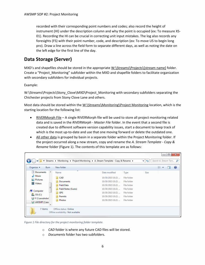
AWSMP SOP #2: Project Monitoring
recorded with their corresponding point numbers and codes; also record the height of instrument (HI) under the description column and why the point is occupied (ex: To measure XS-01). Recording the HI can be crucial in correcting unit input mistakes. The log also records any foresights (FS) with their point number, code, and description (ex: To move US to begin long pro). Draw a line across the field form to separate different days, as well as noting the date on the left edge for the first line of the day.
Data Storage (Server) MXD’s and shapefiles should be stored in the appropriate W:\Streams\Projects\[stream name] folder. Create a “Project_Monitoring” subfolder within the MXD and shapefile folders to facilitate organization with secondary subfolders for individual projects.
Example:
W:\Streams\Projects\Stony_Clove\MXD\Project_Monitoring with secondary subfolders separating the Chichester projects from Stony Clove Lane and others.
Most data should be stored within the W:\Streams\Monitoring\Project Monitoring location, which is the starting location for the following list:
• RIVERMorph File – A single RIVERMorph file will be used to store all project monitoring related data and is saved in the RIVERMorph - Master File folder. In the event that a second file is created due to different software version capability issues, start a document to keep track of which is the most up-to-date and use that one moving forward or delete the outdated one.
• All other data is grouped by basin in a separate folder within the Project Monitoring folder. If the project occurred along a new stream, copy and rename the A. Stream Template - Copy & Rename folder (Figure 1). The contents of this template are as follows:
Figure 1 File directory for the project monitoring folder template.
o CAD folder is where any future CAD files will be stored. o Documents folder has two subfolders.
6
AWSMP SOP #2: Project Monitoring
Monitoring Protocol and XS Info stores many useful and important documents that should be reviewed and/or printed for field use. Files include site specific monitoring instructions, printable maps of monument locations that also serve as field maps, organized photos of monuments, total station file set up instructions, and other monument information (coordinates, elevation, etc.).
Reports is where monitoring reports are saved and is separated into drafts and final versions. JPEGs of maps & figures for the reports are also saved here.
o Field Data is where the survey and pebble count data is saved. Data downloaded from the data logger should be stored under Total
Station\Raw and be separated based on project location and year. Finalized (processed and corrected) data with notes should be saved into two or
three excel documents using the same letter to group project files together. For example: Under Stony Clove Creek, the letter A is designated for the Chichester and Confluence projects while B is used for Stony Clove Lane. This data is saved under Total Station\Finalized.
Total Station\Exported RIVERMorph Graphs stores longitudinal profiles and XS graphs.
o Field Notes (Scans) are for scanned documents separated by project site and year. o GPS is for Trimble GPS files to be stored and is separated by individual projects. o Permits are for ACOE and DEC permits. o Photos are separated by project name. Separate tie-in photos by putting them into a
folder named A. [year] Tie-ins. All other monitoring photos can be placed in a subfolder named B. [year] Monitoring. Also store photos recorded during bankfull or larger flow events in a subfolder named C. [date] and include the approximate recurrence interval.
Data Processing All data will be stored and analyzed using Microsoft Excel 2013, RIVERMorph 5.1.8, ArcGIS 10.2.2, and AutoCAD as available. Below are specific instructions for organizing data and conducting simple analysis using the various software products. For more information on the use of these products, refer to the software user manuals.
1) Cross Sections o Documents being referenced in this section should be within
W:\Streams\Monitoring\Project Monitoring\[stream name]\Field Data\Total Station o Excel Spreadsheets –
a. Data Notes Excel Spreadsheet (finalized folder): Create or update to summarize the data and keep track of any errors encountered. There should be a new tab for different years. For each XS, record the corresponding point numbers (XS and local topo’s separated), the date the data was collected, photo numbers, notes about the data, and any errors detected. Continue to update this document as data is processed.
b. XS and Long Pros Excel Spreadsheet (finalized folder): Create or update. Create a tab for each XS and rename the tabs as such: XS-01 (2015). For each XS, copy the corresponding data points, as recorded in the Data Notes document, from
7
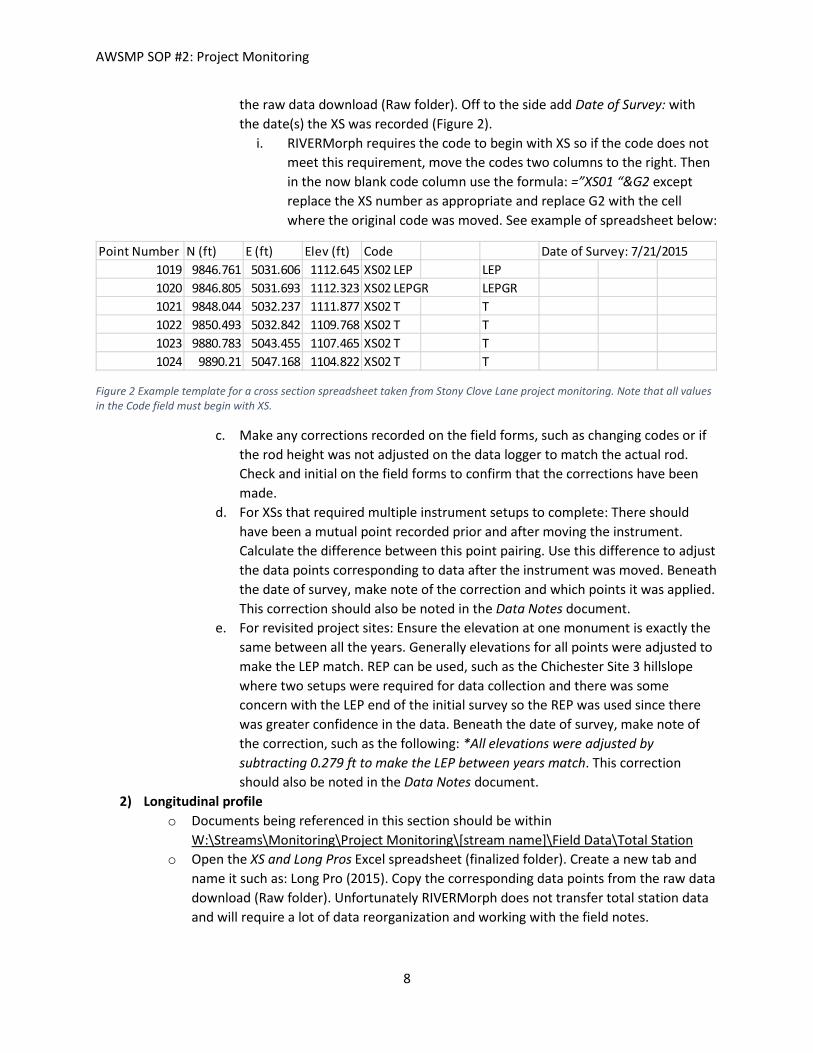
AWSMP SOP #2: Project Monitoring
the raw data download (Raw folder). Off to the side add Date of Survey: with the date(s) the XS was recorded (Figure 2).
i. RIVERMorph requires the code to begin with XS so if the code does not meet this requirement, move the codes two columns to the right. Then in the now blank code column use the formula: =”XS01 “&G2 except replace the XS number as appropriate and replace G2 with the cell where the original code was moved. See example of spreadsheet below:
Figure 2 Example template for a cross section spreadsheet taken from Stony Clove Lane project monitoring. Note that all values in the Code field must begin with XS.
c. Make any corrections recorded on the field forms, such as changing codes or if the rod height was not adjusted on the data logger to match the actual rod. Check and initial on the field forms to confirm that the corrections have been made.
d. For XSs that required multiple instrument setups to complete: There should have been a mutual point recorded prior and after moving the instrument. Calculate the difference between this point pairing. Use this difference to adjust the data points corresponding to data after the instrument was moved. Beneath the date of survey, make note of the correction and which points it was applied. This correction should also be noted in the Data Notes document.
e. For revisited project sites: Ensure the elevation at one monument is exactly the same between all the years. Generally elevations for all points were adjusted to make the LEP match. REP can be used, such as the Chichester Site 3 hillslope where two setups were required for data collection and there was some concern with the LEP end of the initial survey so the REP was used since there was greater confidence in the data. Beneath the date of survey, make note of the correction, such as the following: *All elevations were adjusted by subtracting 0.279 ft to make the LEP between years match. This correction should also be noted in the Data Notes document.
2) Longitudinal profile o Documents being referenced in this section should be within
W:\Streams\Monitoring\Project Monitoring\[stream name]\Field Data\Total Station o Open the XS and Long Pros Excel spreadsheet (finalized folder). Create a new tab and
name it such as: Long Pro (2015). Copy the corresponding data points from the raw data download (Raw folder). Unfortunately RIVERMorph does not transfer total station data and will require a lot of data reorganization and working with the field notes.
Point Number N (ft) E (ft) Elev (ft) Code Date of Survey: 7/21/20151019 9846.761 5031.606 1112.645 XS02 LEP LEP1020 9846.805 5031.693 1112.323 XS02 LEPGR LEPGR1021 9848.044 5032.237 1111.877 XS02 T T1022 9850.493 5032.842 1109.768 XS02 T T1023 9880.783 5043.455 1107.465 XS02 T T1024 9890.21 5047.168 1104.822 XS02 T T
8
AWSMP SOP #2: Project Monitoring
a. At minimum the following columns are needed: Tape (ft), TW (ft) aka CH, WS (ft), and Notes/Code. Add additional column(s) if bankfull and/or top of bank points were collected.
b. Go ahead and delete the northing and easting columns from the copied raw data. Only the point numbers, elevation, and codes are required.
c. For each station/tape value: Look at the field notes for which point numbers correspond to the specific station. Find that point number within the copied raw data set and copy (or move) its corresponding elevation value to the appropriate column (TW vs. WS) based on the field notes. Fill in the code for the station. Once this is complete, any remnants of the copied raw data can be deleted.
i. It may be useful to create outer box borders to separate different data groups. For example: The long pro for Chichester and Confluence projects has Warner Creek, Stony Clove Creek above confluence, and Stony Clove Creek below confluence as three groups.
d. Off to the side add Date of Survey: with the date(s) the long pro was recorded. Also define any codes used, such as U = run, R = riffle, etc.
e. Make a table that calls out the station for each XS. 3) Pebble counts
o An excel document, 0. Pebble Count Calculator, has been created and saved where the pebble count data is stored. Make a copy of this document and rename it for the appropriate year and project site. Simply replace the 100 pebble values with the data collected. The excel spreadsheet is set up to tally the number of pebbles that fall into the different particle size categories, which is the format required by RIVERMorph. Add the date the pebble count was collected.
4) RIVERMorph: Add XSs (as Survey Data), longitudinal profile (Profiles), and pebble count (Particles) data to the master file. Make the necessary graphs for reports and use the Classification tool to calculate Rosgen’s stream type.
5) GPS files: Use GPS Pathfinder Office to correct GPS files and export shapefiles.
House Keeping
The following are tasks to be completed after a project’s initial data collection is complete and processed. Created documents should be stored here: W:\Streams\Monitoring\Project Monitoring\[stream name]\Documents\Monitoring Protocol and XS Info\[project name]. MXDs should be stored here: W:\Streams\Projects\[stream name]\MXD\Project_Monitoring\[project name].
• Monuments_Info provides a summary of benchmarks and XS monuments. Coordinates can be determined from corrected GPS data, XS elevations from the initial total station survey, BM elevations from the As-Built or other reported sources, and compass bearings from the field work. Make note of these data sources. Print a copy for the project monitoring binder.
• TotalStation_FileSetup provides the steps to be followed each year to ensure that the total station is set up the same. It should state what type of coordinate system to use, the elevation and coordinates (likely local coordinates rather than true) for the first occupy point, specify the first occupy point, specify the backsight point and what compass bearing to input, and any
9
AWSMP SOP #2: Project Monitoring
description required if the backsight is not a typical rebar monument. Print a copy for the project monitoring binder.
• XS_LocationPhotos: Gather photos that best depict the monument locations with the intention of assisting the field team in finding them. This means the pictures should not be too close up that you can’t discern anything nearby. There should be a photo of every monument – Make sure to label the monuments (LEP, FPLEP, etc.). Create one page per XS. Print these out single sided so that they can separated within the project monitoring binder.
• Save a JPEG or PDF of the map intended to be used as a future monitoring map. It should depict the XSs and benchmarks/stations. The elevation to be used during total station file setup should also be called out. Save the MXD.
• Create and save MXDs for the monitoring reports: o One for the title page that simply depicts the stream flow direction and extent of the
project area with the most up-to-date aerial imagery. The project extent can be approximate positions and will require a point shapefile to be made. Include basic map elements (scale bar and north arrow).
o A planform map of XS locations. This should include point locations of the XS monuments with a line drawn to depict the XSs. Include labels for the XS names, depict stream flow direction, scale bar, and north arrow.
Data Reporting 1) ACOE Monitoring Reports – Typically, all ACOE permits require submission no later than
October 31 in the first and second years following project completion. At minimum the reports must include:
a. As-built plan and section view drawings. b. Photographs –
i. Of stream channel (within project site and upstream/downstream reaches) and riparian zones affected by project.
ii. Photos taken during normal flow (during data collection is fine) and during or immediately following an annual or bankfull flow event.
c. Reach Classification – Include channel dimensions at bankfull, longitudinal profile of reach, pebble count results, and stream type (Rosgen, 2008).
d. Reach Condition – Written description of observed condition and any corrective measures (with an implementation schedule) required to address any detected instabilities. Include discussion on structure conditions, conditions upstream and downstream of permit area.
e. Recommendations – If poor conditions are reported, include recommendations on needed repairs or project modifications.
f. Vegetation – Regardless if ACOE permit requires vegetation reporting for the specific site, the riparian vegetation section is important as all restoration projects should incorporate re-vegetation. Use CSBI results (if available).
g. Wildlife – Some ACOE permits require reporting wildlife usage. A single paragraph is sufficient (see Stony Clove Creek’s Site 1 report for example).
See examples from other projects while writing the reports. Some things to take notice of:
10

AWSMP SOP #2: Project Monitoring
• Some tables have columns added for each year of monitoring while others have the data displayed for only that particular year.
• Some tables are added for second and later year’s reports. • The vegetation section will report results of CSBI monitoring for corresponding years or
general information on the off years. • The annual flow photos can be excluded if no bankfull events occur that year. In such
cases, add a graph of the streamflow events (using a nearby gage if needed) and mention that there has only been low flows that year.
• The Channel Stability section of the reports are customized to the individual project site, such as including discussion for treated hillslopes.
• Not all project sites require wildlife observations so this section is not present in all reports.
2) Following completion of all ACOE report requirements, reporting detail and frequency objectives are different. Reporting will be more focused on the program goals for that specific project site. Since survey frequency will be less frequent and dependent on flows, reports will only be produced when sufficient data warrants it. Such reports will be simple with a summary of data and calculated changes, contain many graphs/maps exhibiting trends, and provide discussion on project performance.
3) Master Excel Spreadsheet to track all project monitoring and reporting activities and deadlines. Kind of like what Greene County had (see image)…keeps it all organized, especially as we continue to add projects to the list.
11
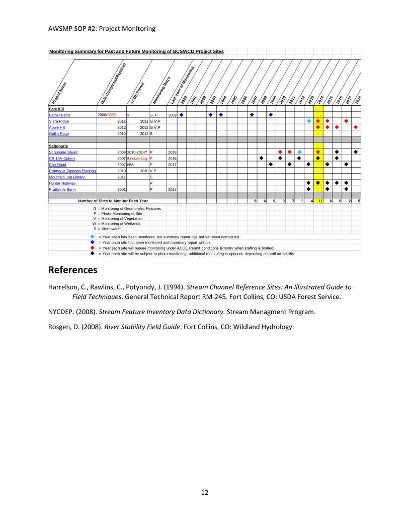
AWSMP SOP #2: Project Monitoring
References Harrelson, C., Rawlins, C., Potyondy, J. (1994). Stream Channel Reference Sites: An Illustrated Guide to
Field Techniques. General Technical Report RM-245. Fort Collins, CO: USDA Forest Service.
NYCDEP. (2008). Stream Feature Inventory Data Dictionary. Stream Managment Program.
Rosgen, D. (2008). River Stability Field Guide. Fort Collins, CO: Wildland Hydrology.
Monitoring Summary for Past and Future Monitoring of GCSWCD Project SitesPr
ojec
t Nam
e
Date
Com
plet
ed/R
epai
red
ACOE
Per
mit
Mon
itorin
g Re
q's
Last
Yea
r of M
onito
ring
2000
2001
2002
2003
2004
2005
2006
2007
2008
2009
2010
2011
2012
2013
2014
2015
2016
2017
2018
East KillFarber Farm 2000/2008 x G, P 2009 Vista Ridge 2011 2011 G,V,P Apple Hill 2013 2012 G,V,P Griffin Road 2012 2012 S
SchoharieSchoharie Street 2009 2010-2014? P 2018 CR 13A Culvert 2007 If necessary P 2016 Carr Road 2007 N/A P 2017 Prattsville Riparian Planting 2010 2010 V,PMountain Top Library 2011 SHunter Highway P Prattsville Berm 2001 P 2017
8 6 9 9 7 9 4 11 6 8 2 5
G = Monitoring of Geomorphic FeaturesP = Photo Monitoring of SiteV = Monitoring of Vegetation
WS = Stormwater
Number of Sites to Monitor Each Year
= Year each site has been monitored and summary report written = Year each site will require monitoring under ACOE Permit conditions (Priority when staffing is limited) = Year each site will be subject to photo monitoring, additional monitoring is optional, depending on staff availability
= Year each has been monitored, but summary report has not yet been completed
= Monitoring of Wetlands
12