New tools for chemical bonding analysis

Eduard Matito

October 13, 2021

Contents

1 Introduction 4

2 Theoretical Background 52.1 The Electron Density . . . . . . . . . . . . . . . . . . . . . . . . . 62.2 The Pair Density . . . . . . . . . . . . . . . . . . . . . . . . . . . 82.3 Electron Correlation . . . . . . . . . . . . . . . . . . . . . . . . . 13

3 The Atom in the Molecule 163.1 The Origin of the Atom . . . . . . . . . . . . . . . . . . . . . . . 163.2 Modern Theory of the Atom . . . . . . . . . . . . . . . . . . . . . 183.3 The definition of an atom in a molecule . . . . . . . . . . . . . . 183.4 Hilbert space partition . . . . . . . . . . . . . . . . . . . . . . . . 193.5 Real space partition . . . . . . . . . . . . . . . . . . . . . . . . . 20

3.5.1 The quantum theory of atoms in molecules (QTAIM) . . 213.5.2 Other real-space partitions . . . . . . . . . . . . . . . . . 293.5.3 References . . . . . . . . . . . . . . . . . . . . . . . . . . . 31

3.6 Population analysis . . . . . . . . . . . . . . . . . . . . . . . . . . 313.6.1 Mulliken population analysis . . . . . . . . . . . . . . . . 313.6.2 Population from real space partitions . . . . . . . . . . . . 323.6.3 The electron-sharing indices (bond orders) . . . . . . . . . 333.6.4 Multicenter Indices . . . . . . . . . . . . . . . . . . . . . . 35

4 Aromaticity 434.1 Global and Local Aromaticity . . . . . . . . . . . . . . . . . . . . 454.2 Geometrical indices . . . . . . . . . . . . . . . . . . . . . . . . . . 454.3 Magnetic indices . . . . . . . . . . . . . . . . . . . . . . . . . . . 464.4 Electronic indices . . . . . . . . . . . . . . . . . . . . . . . . . . . 47

4.4.1 The Aromatic Fluctuation Index: FLU . . . . . . . . . . . 484.4.2 A Multicenter based index: Iring . . . . . . . . . . . . . . 484.4.3 The Multicenter Index: MCI . . . . . . . . . . . . . . . . 494.4.4 The para-Delocalization Index: PDI . . . . . . . . . . . . 494.4.5 The Bond-Order Alternation . . . . . . . . . . . . . . . . 494.4.6 AV1245 and AVmin . . . . . . . . . . . . . . . . . . . . . . 504.4.7 EXERCISE 8 (Aromaticity) . . . . . . . . . . . . . . . . . 51

1

5 Oxidation state 575.1 Definition . . . . . . . . . . . . . . . . . . . . . . . . . . . . . . . 575.2 Computational calculation of Oxidation States . . . . . . . . . . 58

5.2.1 Bond Valence Sum . . . . . . . . . . . . . . . . . . . . . . 585.2.2 Atom Population Analysis . . . . . . . . . . . . . . . . . . 595.2.3 Spin Densities . . . . . . . . . . . . . . . . . . . . . . . . . 595.2.4 Orbital-localization Methods: Effective Oxidation State . 62

6 The Electron Localization Function (ELF) 656.1 The topological analysis of the electron density . . . . . . . . . . 66

7 The local Spin 69

8 Appendices 708.1 Appendix I: How to perform calculations . . . . . . . . . . . . . . 708.2 Appendix II: Manual of ESI-3D . . . . . . . . . . . . . . . . . . . 71

8.2.1 How to cite the program . . . . . . . . . . . . . . . . . . . 718.2.2 Compulsory keywords . . . . . . . . . . . . . . . . . . . . 72

8.3 Optional keywords . . . . . . . . . . . . . . . . . . . . . . . . . . 73

2

Notation

In the following sections we will often deal with coordinates, usually elec-tronic coordinates. The coordinates of an electron in the Cartesian space areindicated by a three-dimensional vector ~r ≡ r (indistinctly indicated by an arrowor a boldfaced number) and the spin polarization (α or β, generically indicatedby the σ). Therefore, many textbooks indicate the coordinates of electron as~x1 or x1, where ~x1 = (~r1, σ1). For the sake of simplification in these notes wehave used the short-hand notation 1 ≡ (~r1, σ1) and d1 ≡ d~r1dσ1 for the electronpositions and their derivates.

N denotes the number of electrons in the system. Ψ is the Greek letterused to represent the electron wavefunction, Ψ(1,2, . . . ,N). φ(1) will be usedto indicate an orbital: an atomic orbital if we use a Greek letter as a subindex,φµ(1), or a molecular orbital if we use a Latin letter, φi(1).

Vectors are indicated in bold or using a superscripted arrow, e.g. , n = ~n =

(nx, ny, nz). Keep in mind that the nabla operator is a vector, ∇ =(

∂∂x ,

∂∂y ,

∂∂z

)

and it can be also indicated as ~∇ in some textbooks.

3

Chapter 1

Introduction

”The theory behind chemistry, which atoms combine with whichat which rate and so forth, is in principle theoretical chemistrydeeply, is physics.”

Audience laughs.

”It is not a joke, it is a direct chemists would admit. That’sexactly their point of view, that atoms in deepest level is physics!Except that the atoms have so many particles that is very hard tocalculate what is going to happen, so they have to use a lot of empir-ical rules to help them. But, as far as we can tell, there is nothingabout chemistry that is not understood ultimately at the behaviorof electrons following the laws of motion of quantum mechanics.”

Richard FeynmannLecture on Quantum ElectroDynamics

Auckland (1979)

This course was designed as part of the subject New Tools for ChemicalBonding Analysis, given in the Master in Advanced Catalysis and MolecularModelling (MACMoM) organized by the Institute of Computational Chemistryand Catalysis (IQCC) at the University of Girona since 2013. This course aimsto introduce chemistry students to the subject of chemical bonding analysisusing tools that are developed in the framework of quantum chemistry. Some ofthese tools have been available in the literature since the mid 90s, while manyothers have been developed in the last fifteen years. The course will first coverthe most elemental concepts of quantum mechanics needed to introduce thetools. However, it assumes a basic knowledge of quantum mechanics (usuallyprovided in the bachelor of chemistry or physics), which includes the structureof the atom, the concept of the wavefunction, the uncertainty, and the Pauliprinciples. We also assume that the reader is familiar with classical chemicalconcepts such as the chemical bond, types of bonds, polarity, ionicity, bondorder, resonant structures or aromaticity.

4

Chapter 2

Theoretical Background

We assume a Born-Oppenheimer quantum mechanics description of anN -electronsystem. This system is completely described by an electronic wavefunction thatdepends on the four coordinates of each electron (1 ≡ (σ1, ~r1): the spin, σi,and the three-dimensional vector, ~r1, giving the position of the electron in theCartesian space) and parameterically on the atomic coordinates. The Slaterdeterminant is the simplest wavefunction in terms of molecular orbitals, φki

(1),respecting the antisymmetric nature of electrons:

ψK

(1,2, . . . ,N)

∣

∣

∣

∣

∣

∣

∣

∣

∣

φk1(1) φk1

(2) . . . φk1(N)

φk2(1) φk2

(2) . . . φk2(N)

......

. . ....

φkN(1) φkN

(2) . . . φkN(N)

∣

∣

∣

∣

∣

∣

∣

∣

∣

The Hartree-Fock (HF) method assumes an approximate wavefunction con-sisting of one Slater determinant. Hence, the HF method is a monodeterminant(or single-determinant) approximation. A typical way to obtain a more accuratedescription of the system involves the use of a wavefunction including a linearcombination of nC Slater determinants,

Ψ(1,2, . . . ,N) =

nC∑

K=1

cKψ

K(1,2, . . . ,N) with

nC∑

K=1

|cK|2 = 1 . (2.1)

The Kohn-Sham density functional theory (KS-DFT) also uses one Slaterdeterminants (although this wavefunction does not correspond to the actual sys-tem). Hereafter, we will refer to the single-determinant (SD) wavefunction asSD-wfn. Wavefunctions composed of more than one Slater determinant are ob-tained from configuration interaction (CI), complete active space self-consistentfield (CASSCF), coupled-cluster (CC), and second-order Moller-Plesset (MP2)methods, [1] among others.a These wavefunctions will be referred as correlatedwavefunctions or multideterminant wavefunctions. The name correlated is given

aIn practice, only CI and CASSCF admit straightforward expansions of the wavefunctionin terms of Slater determinants. CC and MP2 are not variational methods and their energycannot be obtained as the expected value of the Hamiltonian operator using an expansion ofSlater determinants.

5

to emphasize that the latter wavefunctions, unlike SD-wfns, include electroncorrelation (i.e., they go beyond the description offered by HF). b

2.1 The Electron Density

The electron density is the central quantity of density functional theory (DFT) [3]

and the quantum theory of atoms in molecules (QTAIM). [4] Unlike the wave-function, which depends on 3N Cartesian coordinates, the density is actually asimpler quantity that only depends on three Cartesian coordinates. In addition,the density is an observable (a quantity we can measure) that can be experi-mentally obtained from X-ray spectroscopy analysis.

Born’s rule [5] states that the probability density of finding one electron atd1 (the infinitesimal volume around the position of electron 1 with spin σ1) isgiven by the square of the wavefunction that describes the system,

P (1)d1 =

∫

d2

∫

d3 . . .

∫

dN |Ψ(1,2, . . . ,N)|2 d1 , (2.2)

from which we can define the density (also known as density function),

ρ(1) = NP (1) , (2.3)

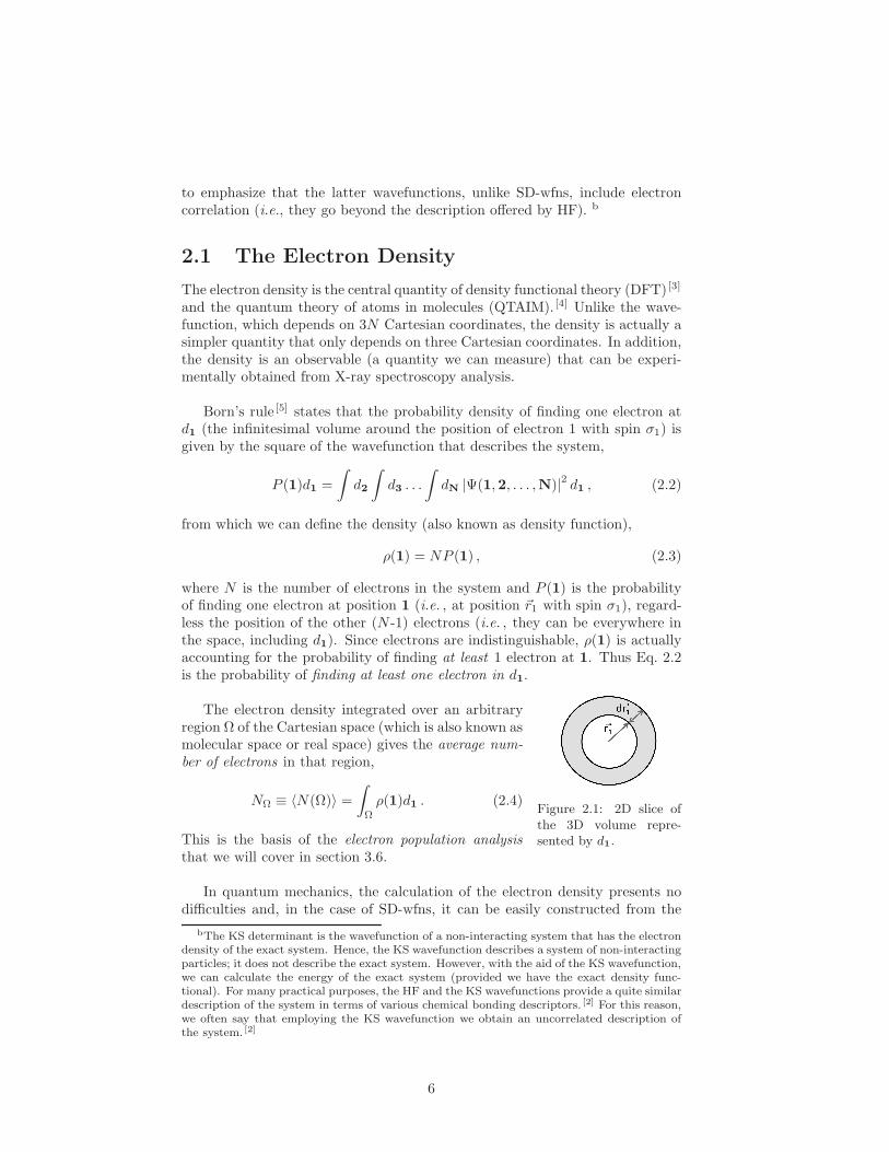
where N is the number of electrons in the system and P (1) is the probabilityof finding one electron at position 1 (i.e. , at position ~r1 with spin σ1), regard-less the position of the other (N -1) electrons (i.e. , they can be everywhere inthe space, including d1). Since electrons are indistinguishable, ρ(1) is actuallyaccounting for the probability of finding at least 1 electron at 1. Thus Eq. 2.2is the probability of finding at least one electron in d1.

Figure 2.1: 2D slice ofthe 3D volume repre-sented by d1.

The electron density integrated over an arbitraryregion Ω of the Cartesian space (which is also known asmolecular space or real space) gives the average num-ber of electrons in that region,

NΩ ≡ 〈N(Ω)〉 =

∫

Ω

ρ(1)d1 . (2.4)

This is the basis of the electron population analysisthat we will cover in section 3.6.

In quantum mechanics, the calculation of the electron density presents nodifficulties and, in the case of SD-wfns, it can be easily constructed from the

bThe KS determinant is the wavefunction of a non-interacting system that has the electrondensity of the exact system. Hence, the KS wavefunction describes a system of non-interactingparticles; it does not describe the exact system. However, with the aid of the KS wavefunction,we can calculate the energy of the exact system (provided we have the exact density func-tional). For many practical purposes, the HF and the KS wavefunctions provide a quite similardescription of the system in terms of various chemical bonding descriptors. [2] For this reason,we often say that employing the KS wavefunction we obtain an uncorrelated description ofthe system. [2]

6

molecular orbitals:

ρ(1) =N∑

i

φ∗i (1)φi(1) =N∑

i

|φi(1)|2 , (2.5)

where we have assumed that the system consists of N electrons occupying Norbitals. For closed-shell systems with doubly-occupied orbitals, the expressionreads:

ρ(1) =

Nα∑

i

|φi(1)|2 +

Nβ∑

i

|φi(1)|2 = 2

N/2∑

i

|φi(1)|2 . (2.6)

The two previous expressions are valid for Hartree-Fock (HF) wavefunctionsor wavefunctions obtained from the Kohn-Sham (KS) formulation of DFT –asthese wavefunctions are composed of a single Slater determinant.c For the sakeof generality, hereafter we will not assume doubly-occupied orbitals.

In the case of correlated wavefunctions, the density cannot be representedby a linear combination of the square of the molecular orbitals (Eq. 2.5). Forcorrelated wavefunctions the density is written as:

ρ(1) =

M∑

ij

1Dijφ

∗i (1)φj(1) (2.7)

where M is the total number of molecular orbitals in our system. 1Dij is known

as the 1-density matrix and it corresponds to the matrix representation of theelectron density in terms of molecular orbitals. This matrix has a diagonal formfor SD-wfns and contains zero in the diagonal for elements greater than N ,

1Dij = δij ∀i, j ≤ N

1Dij = 0 ∀i > N ∨ ∀j > N. (2.8)

It is easy to prove that Eq. 2.7 reduces to Eq. 2.5 for SD-wfns (we just need tosubstitute Eq. 2.8 into Eq. 2.7). For correlated wavefunctions, we can simplifythe calculation of the electron density by using a set of orbitals that diagonalizethe 1-density.d These orbitals are called natural orbitals, ηi(1), and togetherwith their associated occupancies, ni, they define the density

ρ(1) =∑

i

niη∗i (1)ηi(1) (2.12)

cLet us recall that within DFT the density is, in principle, the exact one (in practice weapply some density functional approximation –commonly known as functional– and, therefore,the density is not exact). However, the Kohn-Sham orbitals (and the SD-wfn constructed fromthem) correspond to the fictitious non-interacting system.

d

1DL = Ln n = Diag (n1, . . . , nM ) (2.9)

whereη = Lφ ηi(1) =

X

j

Lijφj(1) (2.10)

andφ = (φ1(1), . . . , φM (1))T η = (η1(1), . . . , ηM (1))T (2.11)

7

Unlike molecular orbitals, natural orbitals do not have an associated energy.Instead, there is an orbital occupancy, ni, associated to it, which can be in-terpreted as the probability that an electron occupies this particular naturalorbital from the orbital set. Notice that Eq. 2.12 is a general expression thatcan be also used for SD-wfns. Indeed, Eq. 2.5 can be retrieved from Eq. 2.12by setting the first N occupancies to one (occupied orbital) and the rest to zero(unoccupied).

Finally, let us give the formula for the first-order reduced density matrix (1-RDM) that will be used to define several chemical bonding tools. The 1-RDMexpression reads:

ρ1(1;1′) = N

∫

d2d3 . . .

∫

dNΨ∗(1,2, . . . ,N)Ψ(1′,2, . . . ,N) , (2.13)

where we have used different coordinates for the first electron of the two wave-functions that are included in the integrand, so that the 1-RDM depends ontwo sets of coordinates. The density, Eq. 2.12, is actually the diagonal part ofthe 1-RDM, i.e. , ρ(1) = ρ1(1;1). In terms of natural orbitals and occupancies,the 1-RDM can be written as

ρ1(1;1′) =∑

i

niη∗i (1)ηi(1

′) , (2.14)

and for SD-wfns we have

ρ1(1;1′) =

N∑

i

φ∗i (1)φi(1′) . (2.15)

Finally, we can represent the electron density and the 1-RDM in terms ofatomic orbitals (AOs).

ρ(1;1′) =

m∑

µν

Pµνφ∗µ(1)φν(1′) , (2.16)

where m is the number of basis functions (number of AOs) and P is simplyknown as the density matrix and is obtained from the molecular orbital coeffi-cients, cµi (see Eq. 3.15),

Pµν =

N∑

i

nicµicνi , (2.17)

where ni is the occupation of the φi(1) molecular orbital.

2.2 The Pair Density

In the literature, the word electron pair (or pairing) is often reserved for elec-trons that are connected and form a bonding pair. In this section, we willshow how by counting the number of electron pairs that can be formed in agiven molecular region and between two molecular regions, we can determine towhich extent the electrons in these regions are localized or contribute to form

8

bonding electron pairs. To this end, we will employ several tools from the sta-tistical analysis of the electron population; these quantities will implicitly countelectron pairs and, hence, will require the pair density.

Born’s interpretation can be further extended to include the pair density,

ρ2(1,2) = N(N − 1)P (1,2) (2.18)

with

P (1,2)d1d2 =

∫

d3 . . .

∫

dNΨ∗(1,2, . . . ,N)Ψ(1,2, . . . ,N)d1d2 (2.19)

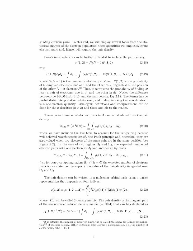
where N(N − 1) is the number of electron pairse and P (1,2) is the probabilityof finding two electrons, one at 1 and the other at 2, regardless of the positionof the other N − 2 electrons. [7] Thus, it represents the probability of finding atleast a pair of electrons: one in d1 and the other in d2. Notice the differencebetween the 1-RDM, Eq. 2.13, and the pair density, Eq. 2.18. The former has noprobabilistic interpretation whatsoever, and —despite using two coordinates—is a one-electron quantity. Analogous definitions and interpretations can bedone for the n-densities (n > 2) and those are left to the reader.

The expected number of electron pairs in Ω can be calculated from the pairdensity:

NΩΩ ≡⟨

N2(Ω)⟩

=

∫

Ω

∫

Ω

ρ2(1,2)d1d2 +NΩ, (2.20)

where we have included the last term to account for the self-pairing becausewell-behaved wavefunctions satisfy the Pauli principle and, therefore, they arezero valued when two electrons of the same spin are in the same position (seeFigure 2.2). In the case of two regions Ω1 and Ω2, the expected number ofelectron pairs with one electron at Ω1 and another at Ω2 reads:

NΩ1Ω2≡ 〈NΩ1

NΩ2〉 =

∫

Ω1

∫

Ω2

ρ2(1,2)d1d2 +NΩ1∩Ω2, (2.21)

i.e. , for non-overlapping regions (Ω1∩Ω2 = ∅) the expected number of electronspairs is calculated as the expectation value of the pair density integrated overΩ1 and Ω2.

The pair density can be written in a molecular orbital basis using a tensorrepresentation that depends on four indices:

ρ(1,2) ≡ ρ2(1,2;1,2) =M∑

ijkl

2Dijklφ

∗i (1)φ∗j (2)φk(1)φl(2) , (2.22)

where 2Dijkl will be called 2-density matrix. The pair density is the diagonal part

of the second-order reduced density matrix (2-RDM) that can be calculated as

ρ2(1,2;1′,2′) = N(N − 1)

∫

d3 . . .

∫

dNΨ∗(1,2, . . . ,N)Ψ(1′,2′, . . . ,N) .

(2.23)

eIt is actually the number of unsorted pairs, the so-called McWeeny (or Dirac) normaliza-tion [6] of the pair density. Other textbooks take Lowdin’s normalization, i.e. , the number ofsorted pairs, N(N − 1)/2.

9

Figure 2.2: Schematic representation of electron pairing within one region A, NAA

(left) and between two regions A and B, NAB (right). Blue lines represent regularelectron pairs and red ones represent self-pairing.

For SD-wfns the 2-RDM (and the pair density) are given by this formula:f

ρSD2 (1,2;1′,2′) =

∣

∣

∣

∣

ρ1(1;1′) ρ1(1;2′)ρ1(2;1′) ρ1(2;2′)

∣

∣

∣

∣

, (2.25)

and

ρSD2 (1,2) =

∣

∣

∣

∣

ρ(1) ρ1(1;2)ρ1(2;1) ρ(2)

∣

∣

∣

∣

= ρ(1)ρ(2) − ρ1(1;2)ρ1(2;1) , (2.26)

where the superscript SD is used to identify expressions that are only valid forSD-wfns.

The calculation of the electronic energy of a molecular system does notrequire the full 2-RDM. The electronic energy of a molecular system is com-posed of three ingredients: the kinetic energy, the electron-nucleus attractionand the electron-electron repulsion. The kinetic energy is a known functional ofthe 1-RDM, the electron-nucleus attraction can be calculated from the electrondensity, whereas the electron-electron repulsion is a well-known functional ofthe pair density. However, from the 2-RDM, we can obtain the 1-RDM and thedensity by reduction of one coordinate and the pair density from its diagonaland, therefore, the electronic energy is a known functional of the 2-RDM. Eventhough the full 2-RDM is not needed to calculate the electronic energy, it isused in other properties. For instance, the calculation of the total angular spinmomentum, 〈S2〉, depends explicitly on the 2-RDM. [8]

Unlike the density, the pair density contains explicit information about therelative motion of electron pairs. In order to extract this information, it iscostumary to define other pair functions. A popular function in DFT is theexchange-correlation density (XCD), [9]

ρxc(1,2) = ρ(1)ρ(2) − ρ2(1,2) , (2.27)

fIn general, a n-RDM can be written in terms of the 1-RDM for a SD-wfn:

ρSDn (1′,2′, . . . ,N′;1,2, . . . ,N) =

˛

˛

˛

˛

˛

˛

˛

˛

˛

ρ1(1′;1) ρ1(1′;2) · · · ρ1(1′;N)ρ1(2′;1) ρ1(2′;2) · · · ρ1(2′;N)

......

. . ....

ρ1(N′; 1) ρ1(N′;2) · · · ρ1(N′;N)

˛

˛

˛

˛

˛

˛

˛

˛

˛

(2.24)

10

which is the difference between the pair density and a fictitious pair density ofindependent electrons that does not satisfy the Pauli principle,

ρIE2 (1,2) = ρ(1)ρ(2) , (2.28)

and gives the probability of finding at least one electron at 1 and, at the sametime, at least one electron at 2. The latter probably is usually greater than theexact pair probability, although this is only strictly necessary for SD-wfns,

ρSDxc (1,2) = ρ(1)ρ(2) − ρSD

2 (1,2) = ρ1(1;2)ρ1(2;1) = |ρ1(1;2)|2 ≥ 0. (2.29)

The XCD is the workhorse for the methods that account for electron localization.One can easily prove that upon integration of the XCD we obtain the density,

∫

ρxc(1,2)d2 = ρ(1), (2.30)

and, therefore, the XCD satisfies this sum rule:

∫ ∫

ρxc(1,2)d1d2 = N. (2.31)

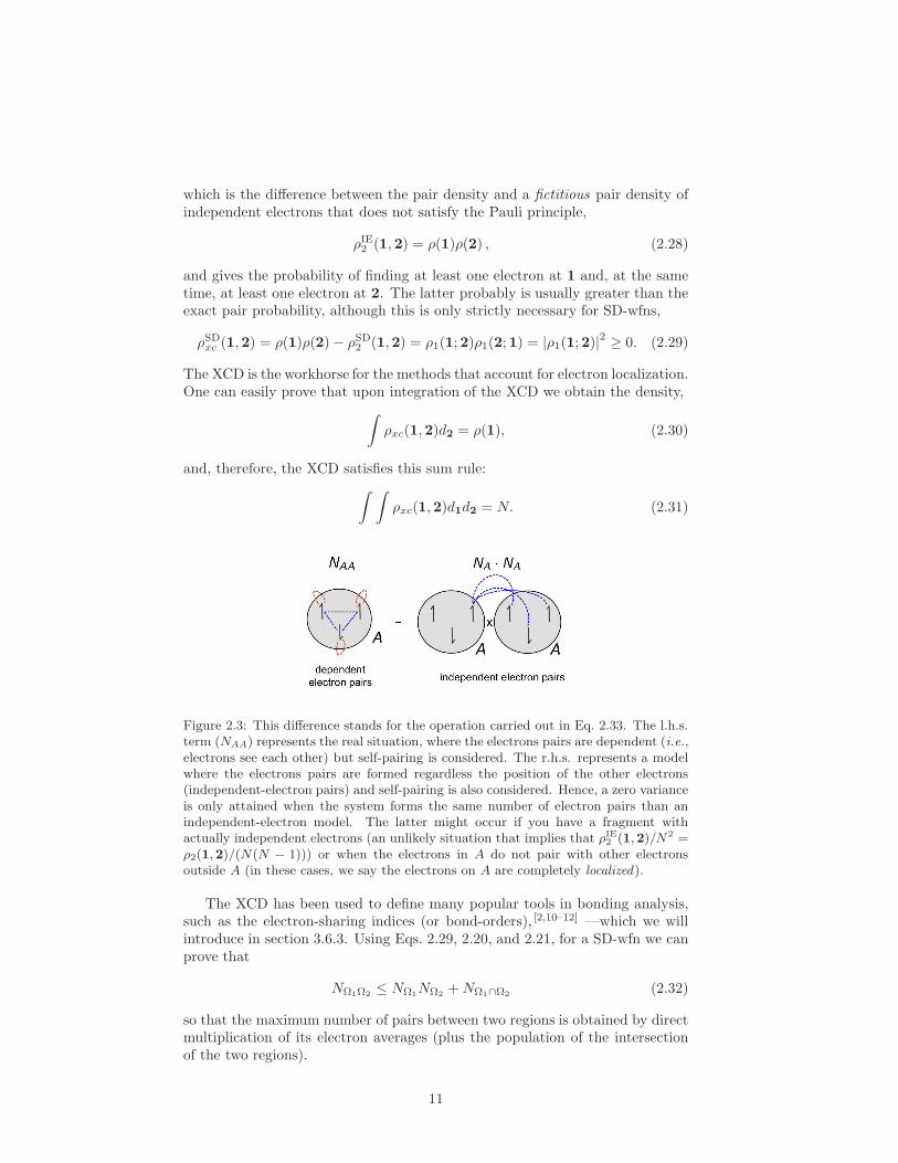
Figure 2.3: This difference stands for the operation carried out in Eq. 2.33. The l.h.s.term (NAA) represents the real situation, where the electrons pairs are dependent (i.e.,electrons see each other) but self-pairing is considered. The r.h.s. represents a modelwhere the electrons pairs are formed regardless the position of the other electrons(independent-electron pairs) and self-pairing is also considered. Hence, a zero varianceis only attained when the system forms the same number of electron pairs than anindependent-electron model. The latter might occur if you have a fragment withactually independent electrons (an unlikely situation that implies that ρIE

2 (1,2)/N2 =ρ2(1,2)/(N(N − 1))) or when the electrons in A do not pair with other electronsoutside A (in these cases, we say the electrons on A are completely localized).

The XCD has been used to define many popular tools in bonding analysis,such as the electron-sharing indices (or bond-orders), [2,10–12] —which we willintroduce in section 3.6.3. Using Eqs. 2.29, 2.20, and 2.21, for a SD-wfn we canprove that

NΩ1Ω2≤ NΩ1

NΩ2+NΩ1∩Ω2

(2.32)

so that the maximum number of pairs between two regions is obtained by directmultiplication of its electron averages (plus the population of the intersectionof the two regions).

11

From the definition of the variance of the number of electrons in Ω

σ2 [NΩ] = NΩΩ −N2Ω (2.33)

using Eq. 2.32 expression we can get an additional relation,

0 ≤ σ2 [NΩ] ≤ NΩ (2.34)

that holds for SD-wfns. The latter inequality puts forward an interesting boundto the uncertainty of the number of electrons in a given region. In particular,from the definition of the variance (and the latter inequality) one can deducethat the uncertainty in the population of a region Ω is only reduced to zerowhen the XCD integrated in Ω equals the number of electrons in this region.Equivalently, we can say that

The minimal uncertainty occurs when the number of electron pairs in Ω isN2

Ω, i.e. , when the electrons in Ω only form pairs among themselves.

Chemically, we would say that the electrons in Ω are localized and do notform pairs with the other electrons in the system, i.e. , Ω is isolated. Hence, themaximal localization of the electrons in Ω occurs for σ2 [NΩ] = 0. Conversely,the variance is maximal when the number of electron pairs in Ω is NΩ(NΩ +1),i.e. , the electrons in Ω form the maximum number of pairs they can amongthemselves (N2

Ω) plus the maximum number of pairs they can form with all theelectrons outside Ω (NΩ), i.e. ,

The uncertainty is maximal when the number of electron pairs in Ω aremaximal NΩ(NΩ + 1), i.e. , all the electrons in Ω are paired with otherelectrons in the system.

In this case, the electrons in Ω reach a situation of minimal localization. Forthese reasons, NΩ−σ

2 [NΩ] can be regarded as a measure of electron localizationin Ω (see Eq. 3.23).

We can also define the covariance of electron populations

cov (NΩ1, NΩ2

) = NΩ1Ω2−NΩ1

NΩ2= NΩ1∩Ω2

−

∫

Ω1

∫

Ω2

ρxc(1,2)d1d2 (2.35)

which measures the dependency between the number of electrons in Ω1 and Ω2.The variance (Eq. 2.33) is actually a special case of the covariance,

σ2 [NΩ] = cov (NΩ, NΩ) (2.36)

and for SD-wfns we can prove the following bound,g

−min(

NΩ1\Ω2, NΩ2\Ω1

)

≤ cov (NΩ1, NΩ2

) ≤ NΩ1∩Ω2. (2.38)

gWe use that for SD-wfns:Z

A

Z

B

ρxc(1, 2)d1d2 = NA −

Z

A

Z

B

ρxc(1,2)d1d2 ≤ NA (2.37)

where B = R3 − B

12

−min (NA, NB) ≤ cov (NA+C , NB+C ) ≤ NC − min (NA, NB) ≤ cov (NA, NB) ≤ 0

Figure 2.4: Venn diagrams for two overlapping regions (left) and two non-overlappingregions (right) and the variance bounds for SD-wfns.

whereΩ1\Ω2 = Ω1 − Ω1 ∩ Ω2

In Figure 2.4, we illustrate the latter inequalities for overlapping and non-overlapping atoms. In addition, one can use the well-known Cauchy-Schwarzinequality to set new bounds

|cov (NΩ1, NΩ2

)| ≤√

σ2 [NΩ1]σ2 [NΩ2

]

As one could anticipate, the minimal covariance between the populations ofΩ1 and Ω2 is given by the number of electrons that are simultaneously in Ω1

and Ω2. Hence,

Zero covariance between regions Ω1 and Ω2 is attained when these regionsdo not overlap and form the maximum possible number of electron pairsbetween them, NΩ1

·NΩ2.

Since electrons interact to each other, this situation only occurs when theelectrons in Ω1 behave as independent of those in Ω2 (and viceversa), i.e. , whenthese two regions do not form bonded electron pairs (see Figure 2.5). Chemically,we say there is no covalent bonding between Ω1 and Ω2. The maximum valueof the covariance is given by smallest number of electrons that are present ineither Ω1 or Ω2. Simply put, we cannot form more bonded electron pairs thanelectrons we have in Ω1 or Ω2.

2.3 Electron Correlation

The term electron correlation was introduced in quantum chemistry in 1934 byWigner and Seitz, [13] when they studied the cohesive energy of metals. Slatercomplained about the fuzziness of the concept and, in 1959, Lowdin gave a soliddefinition of the electron correlation energy [14]

ECORR = EFCI − EHF , (2.39)

where EHF is the Hartree-Fock energy (energy calculated from a SD-wfn) andEFCI is the energy calculated with a full-configuration interaction (FCI) wave-function and, therefore, it is the exact energy of the system. ECORR is called

13

Figure 2.5: This difference stands for the operation carried out in Eq. 2.35. Thel.h.s. term (NAA) represents the real situation, where the electron pairs are dependent(i.e., electrons see each other) but self-pairing is considered. The r.h.s. represents amodel where the electron pairs are formed regardless the position of the other electrons(independent-electron pairs) and self-pairing is also considered.

correlated energy.

We will distinguish between uncorrelated electrons and independent elec-trons. The electrons are uncorrelated if ECORR = 0, whereas electrons areindependent if and only if

ρ2(1,2) =N − 1

Nρ(1)ρ(2) , (2.40)

where the prefactor accounts for the different normalization factors of theindependent-electron pair density (Eq. 2.28) and the actual pair density (Eq. 2.18).The electron correlation energy is a formal definition that measures the energydeviation from a SD-wfn, whereas independent refers to the probabilistic natureof electrons.

It is costumary to define a pair function that measures the deviation of theactual pair density from a pair density of uncorrelated electrons,

λ2(1,2) = ρ2(1,2) − ρSD2 (1,2) = |ρ1(1;2)|2 − ρxc(1,2) (2.41)

and it is usually called the cumulant of the pair density. [15] One can also definethe cumulant of the 2-RDM,

λ2(1,2;1′,2′) = ρ2(1,2;1′,2′) − ρSD2 (1,2;1′,2′) (2.42)

= ρ1(1;2′)ρ1(2;1′) − ρxc(1,2;1′,2′) .

The bounds found in the latter section can now be set for correlated wave-functions in terms of the cumulant matrices,

−min(

NΩ1\Ω2, NΩ2\Ω1

)

− λ2(Ω1,Ω2) ≤ cov (NΩ1, NΩ2

) ≤ NΩ1∩Ω2− λ2(Ω1,Ω2)(2.43)

max (0,−λ2(Ω,Ω)) ≤ σ2[NΩ] ≤ NΩ − λ2(Ω,Ω) , (2.44)

14

whereΩ2 = R

3 − Ω2 = R3\Ω2 , (2.45)

and

λ2(Ω1,Ω2) =

∫

Ω1

∫

Ω2

λ2(1,2)d1d2 . (2.46)

By measuring the importance of λ2 we can assess the importance of electroncorrelation in these quantities. For instance, it is well known that correlationusually decreases the electron fluctuation between different regions [2] and theexperience actually indicates that λ2(Ω,Ω) ≥ 0 and λ2(Ω1,Ω2) ≤ 0. Hence,the electron correlation usually decreases the upper bound of the populationvariance, thus contributing to reduce uncertainty. Electron correlation givesmolecular structures with electrons more localized around the atoms (the vari-ance is smaller) and smaller fluctuation between bonded atomic regions, as weshall see in section 3.6.3.

15

Chapter 3

The Atom in the Molecule

The notion of atom dates back to the fifth century BC and it was conceivedin the ancient Greece. How was it developed? and why? Why did it occur inGreece? To answer these questions we need to go back in time...

3.1 The Origin of the Atom

Twenty five centuries ago most inhabitants of the planet believed that their livesand fates were ruled by a plethora of all-powerful Gods. The actions and the willof these Gods were the most common explanation for the facts that occured inthe world. Back in those days, two major cultures coexisted: the Hebrews (east-ern culture) and the Greeks (western culture). The Hebrews viewed the worldthrough the senses, as opposed to the Greeks, who viewed the world throughthe mind. Although both cultures had great influence in today’s civilization, itwas the Greek culture the one that contributed most to science.

From all cities in the ancient Greece, the idea of the atom was born in themost unexpected one: Abdera. Abdera never had the reputation of other citiesand their inhabitants were often mocked and considered stupid. Although Ab-dera was repeatedly sacked during the course of history, it remained alwayswealthy (so perhaps their citizens were not so stupid after all...). Democritusprobably was its most respected citizen and the father of the atomism theory.

One of the many problems that the Greek philosophers considered was thestudy of the primordial substance, the essential component of the universe. Itis perhaps the first analysis of the structure of matter. Many Greek philoso-phers identified various primitive elements such as fire, water, air, or earth.However, Democritus was the first to consider that everything in nature con-sisted of two elements: the atom and the void. The atoms were conceived aspassive corpuscles, which are incompressible, compact, hard, indestructible, fulland homogeneous. These atoms occupy the void, where they collide with eachother forming clustered structures. Although the atomism theory is mostly at-tributed to Democritus, his mentor (Leucippusa) and Epicurus also contributed.The most important contribution of Epicurus to the atom was the weight. This

aSome authors question the existence of Leucippus.

16

property was used by the opponents of the atomism theory to question it. Theyfound it hard to believe that atoms could form larger structures if their move-ment was vertical as a result of their weight. [16]

It was Lucretius, a Roman philosopher and poet, who furnished Epicurus’theory with the concept of clinamen, providing an explanation for the mecha-nism of atom aggregation. The clinamen is the unpredictable swerve of atomsthat causes the deviation from its vertical trajectories, permitting atom collision.In his words:

”When atoms move straight down through the void by their ownweight, they deflect a bit in space at a quite uncertain time and inuncertain places, just enough that you could say that their motionhas changed. But if they were not in the habit of swerving, theywould all fall straight down through the depths of the void, like dropsof rain, and no collision would occur, nor would any blow be producedamong the atoms. In that case, nature would never have producedanything.”

The concept of atom transcended the structure of matter and it had im-portant significance in philosophy and religion. Democritus stated that the soulwas actually made of atoms and, according to Augustine of Hippo, the clinamenwas the soul of the atom.

Democritus’ idea was far from the actual concept of an atom, but he wasthe first to conceive the atoms as the constituents of nature. Unfortunately, hisideas opposed those of Aristotle and Plato,b which were far more known andrespected in Athens and, consequently, Democritus’ works were mostly ignoredin the ancient Greece. Two hundred years later, Lucretius took them seriouslyand try to polish the atomism theory in his work On the Nature of Things (60BC):

”Observe what happens when sunbeams are admitted into a build-ing and shed light on its shadowy places. You will see a multitude oftiny particles mingling in a multitude of ways... their dancing is anactual indication of underlying movements of matter that are hiddenfrom our sight... It originates with the atoms which move ofthemselves (i.e., spontaneously). Then those small compound bodiesthat are least removed from the impetus of the atoms are set in mo-tion by the impact of their invisible blows and in turn cannon againstslightly larger bodies. So the movement mounts up from the atomsand gradually emerges to the level of our senses, so that those bodiesare in motion that we see in sunbeams, moved by blows that remaininvisible.”

Amazingly, this fragment of the work of Lucretius is considering the randommovement of atoms in what could be considered a first introduction to Brown-ian movement! Brownian motion explains the movement of dust motes or theparticles in a still fluid.

bPlato suggested that the constituents of matter had a precise shape corresponding to thefundamental polyhedra, whereas Aristotle rejected both the theory of his mentor and theatomism theory of Democritus and Epicurus.

17

3.2 Modern Theory of the Atom

In 1807, Dalton, the English chemist and physicist, recovered Democritus’ ideasand formulated the modern atomic theory. Dalton realized that in order tostudy chemistry one should first understand the constituents of matter. Daltonrecognized that chemistry is the study of matter at the atomic level and it isthus often considered the father of chemistry. [4] His ideas went beyond atomismtheory, he assumed that atoms retained their identity even as constituents oflarger structures. Dalton formulated the atoms as indivisible, and his atomictheory provides a formulation of compounds as integer combinations of atoms,introducing the notion of chemical reaction as the process by which atoms arecombined to form molecules.

In 1891, Stoney coined the term electron to name the unit of charge thatshould compose the matter according to Faraday’s electrolysis experiments. Theseries of events that led to the discovery of quantum mechanics were partiallymotivated by the need to suggest a model for the structure of the atom. Theexperiments of Wilhelm, Goldstein, Crookes and Schuster were culminated bythe well-know experiment of J.J. Thompson that proved that atoms are com-posed of electrons and protons.

In 1913, Bohr’s atomic model was formulated, suggesting that electrons inan atom occupy states with quantized energy. In 1916, Lewis suggested thatatoms are held together by sharing a pair of electrons between them, giving afirst (uncompleted) definition of the chemical bond. The notion of electron pairis central in Lewis theory and it remains one of the most important conceptsto explain the chemical bonding. The arrangement of electron pairs in atomsand molecules was also studied and confirmed by other prominent figures in thefield like Langmuir [17] and Pauling. [18]

In 1924, Pauli demonstrated that four quantum numbers are necessary tocharacterize the electrons, thus explaining the shell-like structure of an atom.Actually the contribution of Pauli was the fourth quantum number itself, thespin, an intrinsic property of the electron as proved a year later in the experimentof Uhlenbeck and Goudsmit. The spin of the electrons is actually important inorder to fully understand the chemical bond; the concept of electron pair wouldhave not withstood the new discoveries of the atomic structure without the no-tion of the spin.

3.3 The definition of an atom in a molecule

Since Lewis’ theory, most chemistry has been rationalized using the conceptof an atom in a molecule. For instance, we know from undergraduate organiccourses that carbon binds to itself in many different ways, forming mostly sin-gle, double, triple, and aromatic bonds. Although the carbon atom is the samebuilding block in all these bonds, the character of each carbon is clearly dif-ferent. In order to characterize the electronic structure of these molecules it isconvenient to distinguish and characterize the role of the atoms that form these

18

molecules, i.e., to define an atom in a molecule (AIM).

By characterizing atoms inside a molecule we are defining an atomic parti-tion. An atomic partition (or partitioning) is a well-defined method to subdi-vide the atoms in a molecule. An atomic partition provides the means to defineaverage atomic properties that can be used to (chemically) rationalize the elec-tronic structure of a given molecule; for instance, they are used to define partialcharges, partial multipoles and identify chemical bonds.

There is not a unique way to define an atomic partition and, to some extent,all the proposals are, in one way or another, arbritary. Therefore, it is importantto know the limitations and the drawbacks of the partition we employ. Thereare two ways to define an atomic partition: (i) by partitioning the Hilbert space(the mathematical space where the wavefunction is defined) or (ii) by partition-ing the Cartesian space, i.e. , the space that the molecular structure occupies.

3.4 Hilbert space partition

The solution of the Schrodinger equation is often obtained using approximatewavefunctions expanded by a set of basis functions. The basis set functionsare usually a set of one-particle functions. In principle, one can use any basissets from the Hilbert space to expand a wavefunction: for instance, plane waves(used in solid state) or atomic orbitals constructed from either Slater or Gaus-sian primitive functions. In gas phase or solution, it is customary to employatom-centered functions, making the assignment of the basis set functions toatoms straightforward.

In a Hilbert space partition, the atom in a molecule is defined as the set ofatomic functions centered on that atom. With such a partition, one only needsto decompose the atomic property into basis functions and then it is easy tocalculate the atomic contributions to that property. For instance, if we take thedefinition of a molecular orbital (MO) in terms of atomic orbitals (AOs):

φi(1) ≡ φMOi (1) =

m∑

µ

cµiφAOµ (1) (3.1)

we can choose the part of the MO that corresponds to atom A as the set of mAOs centered in A:

φAi (1) =

m∑

µ∈A

cµiφµ(1) , (3.2)

where we have dropped AO for the sake of convenience. It is easy to prove thatthis assignment provides a partition of the MO:

φMOi (1) =

∑

A

φAi (1) =

∑

A

m∑

µ∈A

cµiφµ(1) . (3.3)

Such atomic decomposition is usually easy to compute and, in particular,the atomic population (see below for a definition) is available in most compu-tational programs under the name of Mulliken population analysis, who first

19

suggested this possibility in 1955. [19]

One of the main advantatges of the Hilbert space partition is that for someproperties, like the atomic populations, the atomic decomposition can be doneanalytically, i.e., it bears no significant computational cost and it can be donewithout committing a numerical error (because the integrals needed can be com-puted analytically). However, the Hilbert space partition presents two majordrawbacks. The first obvious inconvenient is that the method is basis-set de-pendent, i.e., the result is quite dependent on the quality of the basis set usedfor the calculation. The second drawback concerns the ambiguity of assigninga basis set function to an atom. Some atomic basis functions lack a prominentatomic character and, therefore, it is not obvious whether this function can beentirely assigned to one atom. This is the case of diffuse functions, which areassigned to a particular atom but actually are spread over a wider region.

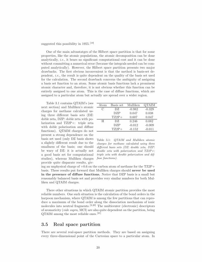
Atom Basis set Mulliken QTAIMC DZ -0.982 -0.329

DZP 0.047 0.038TZ2P+ 0.607 0.047

H DZ 0.246 0.082DZP -0.012 -0.009

TZ2P+ -0.152 -0.011

Table 3.1: QTAIM and Mulliken atomiccharges for methane calculated using threedifferent basis sets (DZ: double zeta, DZP:double zeta with polarization and TZ2P+:triple zeta with double polarization and dif-fuse functions).

Table 3.1 contains QTAIM’s (seenext section) and Mulliken’s atomiccharges for methane calculated us-ing three different basis sets (DZ:doble zeta, DZP: doble zeta with po-larization and TZ2P+: triple zetawith doble polarization and diffusefunctions). QTAIM charges do notpresent a strong dependence on thebasis set used (only DZ basis showsa slightly different result due to thesmallness of the basis; one shouldbe wary of DZ: it is actually nota good basis set for computationalstudies), whereas Mulliken chargesprovide quite disparate results, giv-ing an unphysical charge of +0.6 on the carbon atom of methane for the TZ2P+basis. These results put forward that Mulliken charges should never be usedin the presence of diffuse functions. Notice that DZP basis is a small butreasonably balanced basis set and provides very similar numbers for both Mul-liken and QTAIM charges.

There other situations in which QTAIM atomic partition provides the mostreliable numbers. One such situation is the calculation of the bond orders in theharpoon mechanism, where QTAIM is among the few partitions that can repro-duce a maximum of the bond order along the dissociation mechanism of ionicmolecules into neutral fragments. [2,20] The multicenter (electronic) descriptorsof aromaticity (vide supra, MCI) are also quite dependent on the partition, beingQTAIM among the most reliable ones. [21]

3.5 Real space partition

There are several real-space partition methods. They are based on assigningevery three-dimensional point of the Cartesian space to a particular atom. In

20

Figure 3.1: (left) Richard Bader (1931-2012) from McMaster University is the fatherof the quantum theory of atoms in molecules (QTAIM). (right) A typical molecularplot of QTAIM showing the real-space partition.

some cases, the partition assigns weight functions to every point in the realspace, distributing the importance of the point among the different atoms inthe molecule. Among real space analyses, we can mention Voronoi cells, [22]

Hirshfeld partition, [23] Becke’s partition, [24] Bader’s QTAIM partition, [4] thetopological fuzzy Voronoi cell (TFVC), [25] and Becke-rho methods. [2,26]

3.5.1 The quantum theory of atoms in molecules (QTAIM)

The quantum theory of atoms in molecules (QTAIM) is a very popular theorywhich, among other things, provides a real-space atomic partition. [4] The the-ory is due to Richard F.W. Bader and uses as a central concept the electrondensity. The theory defines the atom through the partitioning of the real spacedetermined by the topological properties of a molecular charge distribution (i.e. ,the electron density, c.f. , Eq. 2.3).

Since the atoms are composed of electrons and most of the chemistry canbe explained by the distribution of the electrons in the molecule, it is naturalto take the electron density as the central quantity to define an atomic partition.

In 1972, Bader and Beddall showed that the atom (or a group of atoms) thathas the same electron distribution makes the same contribution to the total en-ergy of the system. [27] Hence, it makes sense to employ the electron density topartition the Cartesian space and obtain atomic regions. Interestingly, the atomin molecule (AIM) obtained from a density partition are quantum subsystems.Quantum subsystems are open systems defined in real space, their boundariesbeing determined by a particular property of the electronic charge density. [4] Inthe next section, we study how the electron density provides an atomic partitionof the space.

The topological analysis of the electron density

The density is a continuous nonnegative function defined at every point of thereal (Cartesian) space. Therefore, it renders itself to a topological analysis.The calculation of the first derivative of a function provides the set of critical

21

points, rc, of the function ρ(1) (in the present context, we calculate the gradient,because the density depends on three coordinates):

∇ρ(rc) = 0 (3.4)

The characterization of these critical points is done through the analysis of thesecond derivatives of the density at the critical point. All the second derivativesof the density are collected in the so-called Hessian matrix:

H[ρ](rc) = ∇Tr∇rρ(r)

∣

∣

r=rc=

∂2ρ(r)∂x2

∂2ρ(r)∂x∂y

∂2ρ(r)∂x∂z

∂2ρ(r)∂y∂x

∂2ρ(r)∂y2

∂2ρ(r)∂y∂z

∂2ρ(r)∂z∂x

∂2ρ(r)∂y∂z

∂2ρ(r)∂z2

r=rc

(3.5)

that is a real symmetric matrix and thus can be diagonalized through a unitarytransformation, L,

H[ρ]L = LΛ (3.6)

i.e., put in a diagonal form,

Λ =

∂2ρ(r)∂x2

1

0 0

0 ∂2ρ(r)∂y2

1

0

0 0 ∂2ρ(r)∂z2

1

r1=rc

=

λ1 0 00 λ2 00 0 λ3

(3.7)

where (λ1 ≤ λ2 ≤ λ3) are the three eigenvalues of the Hessian matrix, i.e., thecurvatures. We will label each critical point as (ω, σ) according to its rank andsignature, respectively. Assuming non-zero eigenvalues we can classify the CPby the sign of its curvatures. Each positive curvature contributes +1 to thesignature and every negative curvature adds -1, giving four different CPs:

• (3,-3). Attractor or Nuclear Critical Point (ACP). All the cur-vatures are negative in a ACP, and thus this CP is a maximum of theelectron density. These points usually coincide with an atomic position.An atom-in-molecule within QTAIM is characterized by one and only oneACP. Although it is not usual, one may encounter maxima of the electrondensity which do not coincide with an atomic position; those are knownas non-nuclear maxima (NNA). [4,28]

• (3,-1). Bond Critical Point (BCP). A BCP presents two negativecurvatures and a positive one. The BCP is found between two ACPs.The positive eigenvalue (λ3) corresponds to the direction connecting thesetwo ACPs and the negative eigenvalues form a plane in the perpendiculardirection. The existence of a BCP is often used as an indicator of thepresence of a chemical bond between the atoms identified by the two ACPs(see controversy below).

• (3,+1) Ring Critical Point (RCP). A RCP has two positive curvaturesand one negative one (λ1). Its presence indicates a ring structure in theplane formed by the positive eigenvalues. If the molecule is planar theRCP is located in the minimum of the electron density inside the ringstructure.

22

• (3,+3) Cage Critical Point (CCP). A CCP has three negative eigen-values and it is thus a minimum of the electron density. Its presence in-dicates a cage structure and the CCP is usually found close to the centerof cage.

The topology of electron density satisfies the Poincare-Hopf expression,c thatgives the relationship between the number of critical points:

nACP − nBCP + nRCP − nCCP = 1 (3.8)

If after performing the critical point search the number of points does not satisfythe latter expression we should look carefully at the structure and try to locatethe missing critical points.

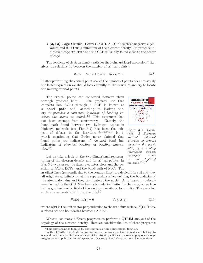
Figure 3.2: Chem-istry, A EuropeanJournal publisheda series of articlesdicussing the possi-bility of a bondinginteraction betweenhydrogens atomsin the biphenylmolecule. [29–32]

The critical points are connected between themthrough gradient lines. The gradient line thatconnects two ACPs through a BCP is known asa bond path and, according to Bader’s the-ory it provides a universal indicator of bonding be-tween the atoms so linked. [33] This statement hasnot been exempt from controversy. Namely, thebond path found between two hydrogen atoms inbiphenyl molecule (see Fig. 3.2) has been the sub-ject of debate in the literature. [29–32,34,35] It isworth mentioning that Bader never claimed thatbond paths are indicators of chemical bond butindicators of chemical bonding or bonding interac-tion. [36]

Let us take a look at the two-dimensional represen-tation of the electron density and its critical points. InFig. 3.3, we can see the density countor plots and the po-sition of ACPs, BCPs, and the bond path of NaCl. Thegradient lines (perpendicular to the countor lines) are depicted in red and theyall originate at infinity or at the separatrix surface defining the boundaries ofthe atomic domains and they terminate at the nuclei. An atom in a molecule—as defined by the QTAIM— has its boundaries limited by the zero-flux surfacein the gradient vector field of the electron density or by infinity. The zero-fluxsurface or separatrix, S(r), is given by: [4]

∇ρ(r) · n(r) = 0 ∀r ∈ S(r) (3.9)

where n(r) is the unit vector perpendicular to the zero-flux surface, S(r). Thesesurfaces are the boundaries betweens AIMs.d

We can use many different programs to perform a QTAIM analysis of thetopology of the electron density. Here we consider the use of three programs:

cThis relationship is fulfilled by any continuous three-dimensional function.dWithin QTAIM, the AIMs do not overlap, i.e. , a given point in the real space belongs to

one and only one atom in the molecule. Other atomic partitions, the overlapping ones, assignweights to each point in the real space; in this case, points belong to more than one atom.

23

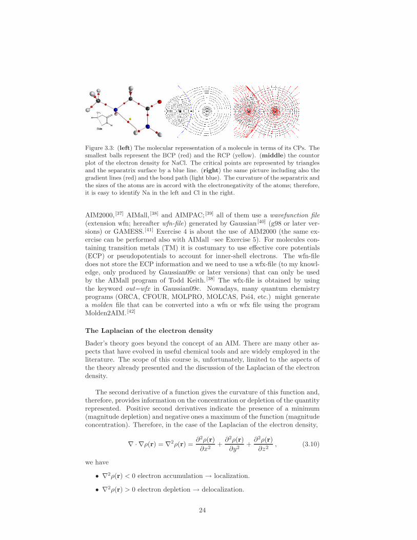
Figure 3.3: (left) The molecular representation of a molecule in terms of its CPs. Thesmallest balls represent the BCP (red) and the RCP (yellow). (middle) the countorplot of the electron density for NaCl. The critical points are represented by trianglesand the separatrix surface by a blue line. (right) the same picture including also thegradient lines (red) and the bond path (light blue). The curvature of the separatrix andthe sizes of the atoms are in accord with the electronegativity of the atoms; therefore,it is easy to identify Na in the left and Cl in the right.

AIM2000, [37] AIMall, [38] and AIMPAC; [39] all of them use a wavefunction file(extension wfn; hereafter wfn-file) generated by Gaussian [40] (g98 or later ver-sions) or GAMESS. [41] Exercise 4 is about the use of AIM2000 (the same ex-ercise can be performed also with AIMall –see Exercise 5). For molecules con-taining transition metals (TM) it is costumary to use effective core potentials(ECP) or pseudopotentials to account for inner-shell electrons. The wfn-filedoes not store the ECP information and we need to use a wfx-file (to my knowl-edge, only produced by Gaussian09c or later versions) that can only be usedby the AIMall program of Todd Keith. [38] The wfx-file is obtained by usingthe keyword out=wfx in Gaussian09c. Nowadays, many quantum chemistryprograms (ORCA, CFOUR, MOLPRO, MOLCAS, Psi4, etc.) might generatea molden file that can be converted into a wfn or wfx file using the programMolden2AIM. [42]

The Laplacian of the electron density

Bader’s theory goes beyond the concept of an AIM. There are many other as-pects that have evolved in useful chemical tools and are widely employed in theliterature. The scope of this course is, unfortunately, limited to the aspects ofthe theory already presented and the discussion of the Laplacian of the electrondensity.

The second derivative of a function gives the curvature of this function and,therefore, provides information on the concentration or depletion of the quantityrepresented. Positive second derivatives indicate the presence of a minimum(magnitude depletion) and negative ones a maximum of the function (magnitudeconcentration). Therefore, in the case of the Laplacian of the electron density,

∇ · ∇ρ(r) = ∇2ρ(r) =∂2ρ(r)

∂x2+∂2ρ(r)

∂y2+∂2ρ(r)

∂z2, (3.10)

we have

• ∇2ρ(r) < 0 electron accumulation → localization.

• ∇2ρ(r) > 0 electron depletion → delocalization.

24

Figure 3.4 illustrates the Laplacian of the density for N2 molecule. In the contourplot, we can appreciate large negative values (large localization of electrons)close to the nuclei and in the bonding region above the intermolecular axis.The latter corresponds to the π-electrons of the bond in N2. These featuresare revealed when we choose a medium-range contour value (the largest valuescorrespond to the nuclei). Contour pictures can be obtained from AIM2000and AIMall (see below). This isosurface dimensional representation has beendone with Molekel [43] (using a cube file including Laplacian values) but it couldbe also done with Vmd [44] (cube file), with molden [45] (using a log file fromGaussian [40] with the gfinput and Iop(6/7=-3) keywords) or with AIMall.

Figure 3.4: The N2 molecule: (left) Contour plot of the negative values (concentrationof charge) of the Laplacian of the density. (right) isosurface representation of ∇2ρ(r)at −0.004.

EXERCISE 4 (AIM2000)

Perform a full topological study of a molecule of your choice. Pick up a moleculewith, at least, a ring structure and draw the molecular representation (3D) andthe contour plot of the electron density. Include critical points, bond paths,separatrices and gradient lines when possible. Perform integrations over atomicregions to obtain some atomic properties. Follow these steps:

1.- Run a Gaussian calculation with the keyword out=wfn to obtain a wfn-file. Here a Gaussian input example:

25

Figure 3.5: Gaussian input to obtain a wavefunction file for the H2 molecule. Noticethe blank lines (marked by blue left square brackets, which should not be included inthe input) before and after the wavefunction file name.

2.- Open the wfn-file with AIM2000. Calculate first the CPs and bond pathsin the molecular representation (they show up in the black window whereyou can freely rotate the molecule to visualize them).

Figure 3.6: Snapshot of AIM2000 program and the most interesting features.

26

Figure 3.7: Molecular representation of benzene. The atoms (C in black, H in lightgrey), the BCPs (red), the RCP (yellow) and the paths connecting the CP are pre-sented.

3.- In the plot menu select contour plot and construct a contour plot like thisone below:

Figure 3.8: The contour plot of the electron density of benzene (contour lines given inblack). The molecule is composed of carbon atoms (dark blue) and hydrogens (lightgrey). The BCPs (red), the RCP (green) and the bond paths (dark blue) connectingC-C and C-H are also given. In brown we can see the separatrix surfaces as theyintersect the molecular plane. The spaces between separatrix surfaces (that extent toinfinity in H atoms) define the AIMs.

4.- Property calculation: Select the atoms you want and perform the integra-tion over them (make sure to integrate in natural coordinates).

27

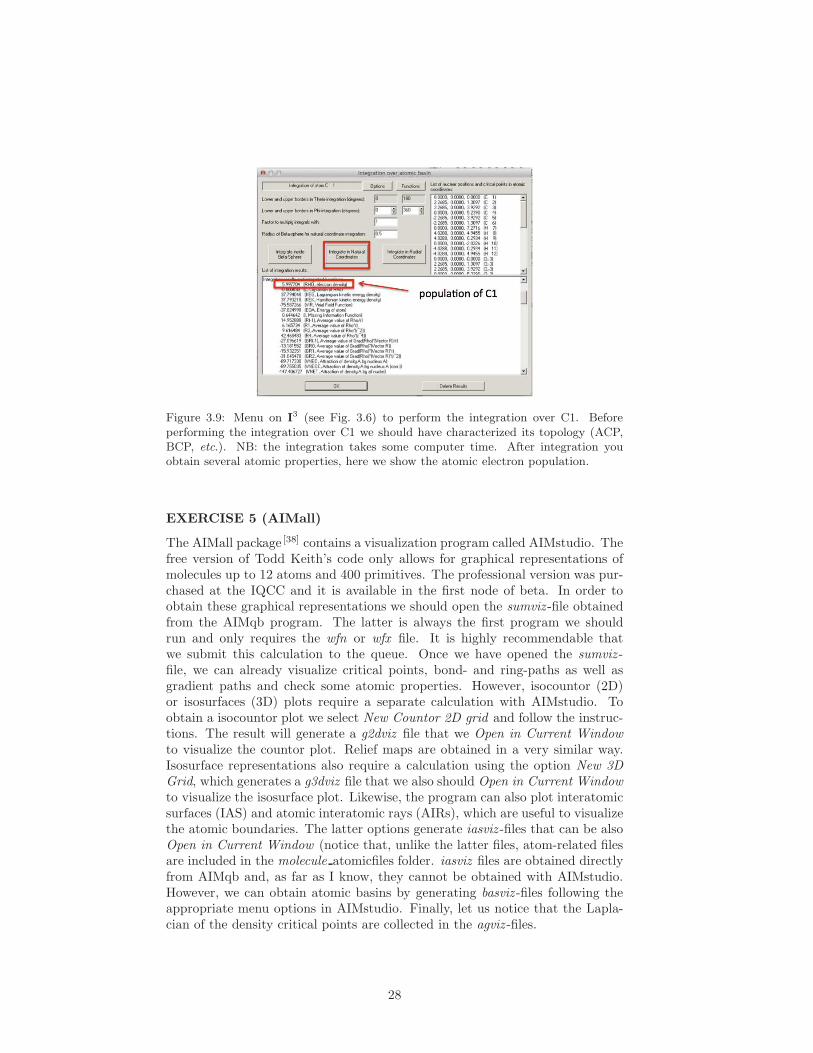
Figure 3.9: Menu on I3 (see Fig. 3.6) to perform the integration over C1. Beforeperforming the integration over C1 we should have characterized its topology (ACP,BCP, etc.). NB: the integration takes some computer time. After integration youobtain several atomic properties, here we show the atomic electron population.

EXERCISE 5 (AIMall)

The AIMall package [38] contains a visualization program called AIMstudio. Thefree version of Todd Keith’s code only allows for graphical representations ofmolecules up to 12 atoms and 400 primitives. The professional version was pur-chased at the IQCC and it is available in the first node of beta. In order toobtain these graphical representations we should open the sumviz -file obtainedfrom the AIMqb program. The latter is always the first program we shouldrun and only requires the wfn or wfx file. It is highly recommendable thatwe submit this calculation to the queue. Once we have opened the sumviz -file, we can already visualize critical points, bond- and ring-paths as well asgradient paths and check some atomic properties. However, isocountor (2D)or isosurfaces (3D) plots require a separate calculation with AIMstudio. Toobtain a isocountor plot we select New Countor 2D grid and follow the instruc-tions. The result will generate a g2dviz file that we Open in Current Windowto visualize the countor plot. Relief maps are obtained in a very similar way.Isosurface representations also require a calculation using the option New 3DGrid, which generates a g3dviz file that we also should Open in Current Windowto visualize the isosurface plot. Likewise, the program can also plot interatomicsurfaces (IAS) and atomic interatomic rays (AIRs), which are useful to visualizethe atomic boundaries. The latter options generate iasviz -files that can be alsoOpen in Current Window (notice that, unlike the latter files, atom-related filesare included in the molecule atomicfiles folder. iasviz files are obtained directlyfrom AIMqb and, as far as I know, they cannot be obtained with AIMstudio.However, we can obtain atomic basins by generating basviz -files following theappropriate menu options in AIMstudio. Finally, let us notice that the Lapla-cian of the density critical points are collected in the agviz -files.

28

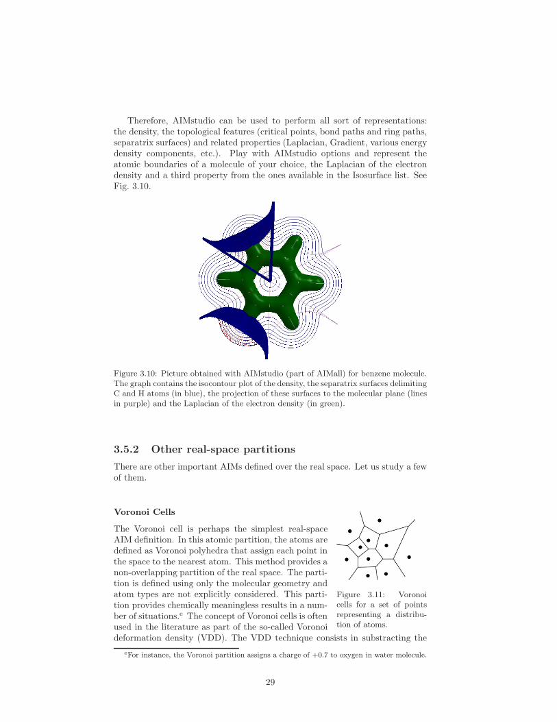
Therefore, AIMstudio can be used to perform all sort of representations:the density, the topological features (critical points, bond paths and ring paths,separatrix surfaces) and related properties (Laplacian, Gradient, various energydensity components, etc.). Play with AIMstudio options and represent theatomic boundaries of a molecule of your choice, the Laplacian of the electrondensity and a third property from the ones available in the Isosurface list. SeeFig. 3.10.

Figure 3.10: Picture obtained with AIMstudio (part of AIMall) for benzene molecule.The graph contains the isocontour plot of the density, the separatrix surfaces delimitingC and H atoms (in blue), the projection of these surfaces to the molecular plane (linesin purple) and the Laplacian of the electron density (in green).

3.5.2 Other real-space partitions

There are other important AIMs defined over the real space. Let us study a fewof them.

Voronoi Cells

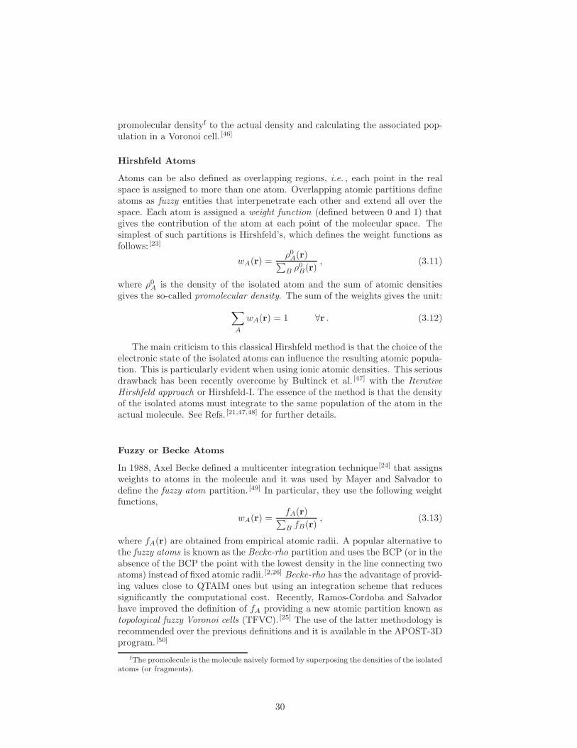
Figure 3.11: Voronoicells for a set of pointsrepresenting a distribu-tion of atoms.

The Voronoi cell is perhaps the simplest real-spaceAIM definition. In this atomic partition, the atoms aredefined as Voronoi polyhedra that assign each point inthe space to the nearest atom. This method provides anon-overlapping partition of the real space. The parti-tion is defined using only the molecular geometry andatom types are not explicitly considered. This parti-tion provides chemically meaningless results in a num-ber of situations.e The concept of Voronoi cells is oftenused in the literature as part of the so-called Voronoideformation density (VDD). The VDD technique consists in substracting the

eFor instance, the Voronoi partition assigns a charge of +0.7 to oxygen in water molecule.

29

promolecular densityf to the actual density and calculating the associated pop-ulation in a Voronoi cell. [46]

Hirshfeld Atoms

Atoms can be also defined as overlapping regions, i.e. , each point in the realspace is assigned to more than one atom. Overlapping atomic partitions defineatoms as fuzzy entities that interpenetrate each other and extend all over thespace. Each atom is assigned a weight function (defined between 0 and 1) thatgives the contribution of the atom at each point of the molecular space. Thesimplest of such partitions is Hirshfeld’s, which defines the weight functions asfollows: [23]

wA(r) =ρ0

A(r)∑

B ρ0B(r)

, (3.11)

where ρ0A is the density of the isolated atom and the sum of atomic densities

gives the so-called promolecular density. The sum of the weights gives the unit:

∑

A

wA(r) = 1 ∀r . (3.12)

The main criticism to this classical Hirshfeld method is that the choice of theelectronic state of the isolated atoms can influence the resulting atomic popula-tion. This is particularly evident when using ionic atomic densities. This seriousdrawback has been recently overcome by Bultinck et al. [47] with the IterativeHirshfeld approach or Hirshfeld-I. The essence of the method is that the densityof the isolated atoms must integrate to the same population of the atom in theactual molecule. See Refs. [21,47,48] for further details.

Fuzzy or Becke Atoms

In 1988, Axel Becke defined a multicenter integration technique [24] that assignsweights to atoms in the molecule and it was used by Mayer and Salvador todefine the fuzzy atom partition. [49] In particular, they use the following weightfunctions,

wA(r) =fA(r)

∑

B fB(r), (3.13)

where fA(r) are obtained from empirical atomic radii. A popular alternative tothe fuzzy atoms is known as the Becke-rho partition and uses the BCP (or in theabsence of the BCP the point with the lowest density in the line connecting twoatoms) instead of fixed atomic radii. [2,26] Becke-rho has the advantage of provid-ing values close to QTAIM ones but using an integration scheme that reducessignificantly the computational cost. Recently, Ramos-Cordoba and Salvadorhave improved the definition of fA providing a new atomic partition known astopological fuzzy Voronoi cells (TFVC). [25] The use of the latter methodology isrecommended over the previous definitions and it is available in the APOST-3Dprogram. [50]

fThe promolecule is the molecule naively formed by superposing the densities of the isolatedatoms (or fragments).

30

3.5.3 References

Recommended bibliography: Bader’s book, [4] Bader’s reviews [51,52] and thenotes of Angel Martin-Pendas in Ref. 53. We will use AIM2000 [37] and AIMall [38]

programs for the visual representations. For a historical account you can readAtkins’ [54] or simply browse the relevant concepts in Wikipedia.

3.6 Population analysis

The population analysis is a technique in computational chemistry that assignsan average number of electrons, the atomic population, to each AIM. Therefore,it is a way to distribute the N electrons in a molecule among their constituentparts. It is costumary to give also the atomic charge, which is calculated as theatomic population minus the atomic number (ZA), i.e.,

QA = ZA −NA . (3.14)

The population analysis is carried out using a certain definition of AIM.Therefore, there are as many population schemes as atomic partitions. Atomiccharges obtained from population analysis should not be used for the calculationof oxidation states. The population analysis provides an average number, whichis often a non-integer value, whereas oxidation states (except for mixed-valencecomplexes) are always integer numbers. One could take the closest integernumber to the atomic population to provide an estimate of the oxidation state.However, this strategy often produces wrong oxidation states. See section 5 forfurther details of the calculation of oxidation states.

Population analyses are very sensible to the choice of the AIM. Therefore, thecalculation of atomic charges using two different methods often yields disparateresults. In this sense, I would not recommend to draw conclusions about theelectronic structure of a molecule based only on atomic charge calculations. [46]

3.6.1 Mulliken population analysis

The most popular population analysis is performed using the Hilbert spacepartition (see above). It is straightforward to calculate and thus it is availablein any computational chemistry code. The definition uses the expression of theelectron density in terms of the set of atomic orbitals (basis set) employed inthe calculation. Assuming m basis functions (AOs), a MO can be expanded interms of these AOs,

φMOi (1) =

m∑

µ

cµiφAOµ (1) . (3.15)

Its squared value reads

|φi(1)|2 =

m∑

µν

cµicνiφ∗µ(1)φν(1) , (3.16)

31

and using the definition of the electron density, Eq. 2.12, we get:

N =

∫

ρ(1)d1 =

N∑

i

ni

∫

|φi(1)|2 d1 =

N∑

i

m∑

µν

cµicνini

∫

φ∗µ(1)φν(1)d1

=

m∑

µν

(

N∑

i

cµicνini

)

∫

φ∗µ(1)φν(1)d1 =

m∑

µν

PµνSµν = Tr (P · S) (3.17)

where P (see Eq. 2.17) and S are the density matrix (in AOs) and the overlapmatrix, respectively. The Mulliken population of atom A is defined as

NA =∑

µ∈A

m∑

ν

PµνSµν . (3.18)

The latter can be easily separated into gross orbital populations, NµA, which

provide the contribution of each orbital, φµ, to the atomic population, NA.

NµA =

m∑

ν

PµνSµν ∀µ ∈ A (3.19)

Since the Mulliken population analysis can be donde separately for α and βelectrons, it is straightforward to obtain spin population analysis. The latterare obtained from the difference of α and β atomic populations,

NsA = Nα

A −NβA (3.20)

Unlike regular atomic populations, which are very sensitive to the atomicpartition, the spin population analysis is a more robust quantity which is quiteuseful, among other things, to identify radicals, unpaired electrons, and —withthe help of the crystal field theory— to determine the oxidation state of AIMs(see section 5.2.3).

The values of Mulliken populations and charges can be found in the output ofGaussian if we use the keyword pop=full. The results of Mulliken populationanalysis have no numerical error associated because they come from an integral(Sµν) that can be performed analytically for gaussian functions. Most compu-tational chemistry codes (Gaussian, GAMESS, NWCHEM, QCHEM, etc.) usegaussian functions as basis sets.

3.6.2 Population from real space partitions

The calculation of populations from a real space partition is more complicatedthan in the Hilbert space case. In the real space, we often need to perform anumerical integration over the atomic domain of A:

NA =

∫

A

ρ(1)d1 =∑

i

ni

∫

A

|φi(1)|2 d1 =∑

i

niSii(A) (3.21)

that requires the diagonal part of the atomic overlap matrix (AOM):

Sij(A) =

∫

A

φ∗i (1)φj(1)d1 .

32

Unless the shape of the AIMs is regular, the calculation of the AOMs requires anumerical integration. The computational cost and the numerical error associ-ated to the population analysis corresponds to the error in the calculation of thecorresponding AOMs. Therefore, it is highly recommended to check the accu-racy of the integration after such analysis. The QTAIM population analysis canbe obtained from AIMall, [38] AIM2000 (see Figure 3.9), using APOST-3D, [50] orESI-3D [55] (ESI-3D does not perform integrations, AOMs should be provided).

3.6.3 The electron-sharing indices (bond orders)

The concept of bond order is crucial to understand the bonding in moleculesand it measures the number of chemical bonds between a pair of atoms. Inhis seminal work, Coulson [56] put forward a measure of the order of a bond,which he applied within Huckel molecular orbital (HMO) theory to explain theelectronic structure of some polyenes and aromatic molecules. This measureis nowadays known as Coulson bond order (CBO) and it is calculated in thecontext of the HMO theory.

Nowadays, very few calculations are performed within the HMO method,as more sophisticated (computational affordable) methods are easily available.As a consequence, the CBO has been replaced by what we could call electronsharing indices (ESI), which measure at which extent two atoms are sharing theelectrons lying between them.

In this course, we will study the ESI that are calculated from the so-calledXCD (Eq. 2.27) and intuitevely arise from the covariance of atomic populations(see Eq. 2.35 and section 2.2).g In the context of QTAIM, the ESI that arisesfrom the population covariance is known as the delocalization index (DI): [10–12]

δ(A,B) = 2

∫

A

∫

B

d1d2ρxc(1,2) = −2cov (NA, NB) . (3.22)

Cmpare the latter to Eq. 2.35 and keep in mind that QTAIM’s AIMs are non-overlapping. Additionally, the XCD can be used to define the localization index(LI), [10]

λ(A) = NA − σ2 [NA] =

∫

A

∫

A

d1d2ρxc(1,2) , (3.23)

which takes values between zero and NA. Since the ESI is defined from thecovariance of the populations of atoms A and B, it is a measure of the numberof electrons simultaneously fluctuating between these atoms. It is costumaryto take this value as the number of electron pairs shared between atoms A andB, a quantity commonly known as the order of the bond or simply bond order. [56]

gThe XCD compares a fictitious pair density of independent electron pairs [ρ(1)ρ(2)] withthe real pair density, ρ2(1, 2) [see Eq. 2.18]. The smaller the difference, the more independentthe electrons in these positions are. The larger the difference, the more dependent, i.e., themore coupled (paired!) they are. Therefore, for pairs of electrons shared between pointsbelonging to two different atoms we expect a large XCD value.

33

Since the XCD integrates to the number of electrons, we can classify theelectrons as localized or delocalized and assign them to atoms or pairs of atoms,respectively. The following sum rule is satisfied:

N =∑

A

NA =∑

B,A<B

δ(A,B) +∑

A

λ(A) (3.24)

An electron totally localized within an atom contributes 1 to the localizationindex. A localized pair of electrons contributes 2 to the localization index andan electron shared between two atoms contributes 1/2 to the localization indexand 1/2 to the delocalization index. [10]

Figure 3.12: The N2 molecule: (left) The Lewis structure. (right) Distribution ofelectrons as localized and delocalized.

Let us take a look at N2. N has a configuration like this: 1s22s22p3 and N2

has a triple bond (2 × 2p3). Each nitrogen has a lone pair (2s2) and two coreelectrons (1s2). There is a total of 14 electrons that can be thus distributed as3 delocalized (each of the 3 electrons shared by each nitrogen contribute 1/2,i.e., 2 × 3 × 1/2) and 5.5 localized (2 come from the lone pair, 2 from the corepair and 3 × 1/2 from each electron shared). This would be the distributionof a perfect Lewis picture of N2. The numbers in Fig. 3.12 are fairly close tothis counting, so the classical Lewis picture agrees with the quantum chemistrydescription of N2. It will not always be the case, as we shall see later on. Ingeneral, single, double, and triple bonds usually exhibit DI values close to 1, 2,and 3, respectively. Aromatic bonds show DI values around 1.5. These valuesare a good indication for simple wavefunctions (such as those obtained from HFor KS wavefunction), whereas correlated wavefunctions usually provide smallerDI values.

It is worth defining the total delocalization in a given atom,

δ(A) =1

2

∑

B 6=A

δ(A,B) (3.25)

which some authors [57] identify with the valence of an atom, and provides anatural division of the number of electrons in an atom,

.NA = δ(A) + λ(A) (3.26)

The bounds stablished in Section 2.2 for the variance and the covarianceprovide useful bounds for the ESIs

0 ≤ δ(A,B) ≤ 2min(NA, NB) (3.27)

0 ≤ λ(A) ≤ NA (3.28)

34

In the case of correlated wavefunctions (see section 2.3), the bounds becomemore convoluted,

δc(A,B) ≤ δ(A,B) ≤ 2min(NA, NB) + δc(A,B) (3.29)

max(λc(A), 0) ≤ λ(A) ≤ NA + λc(A) (3.30)

where λc(A) and δc(A,B) are the correlated parts of the ESI, calculated byreplacing ρxc by λ2 (Eq. 2.41) in Eqs. 3.22 and 3.23.

The DI measures the number of electron pairs covalently shared betweentwo atoms. If the atom pair is bonded by other means (e.g. , by electrostaticinteractions), the index will not reflect this fact. The DI of an ionic bondshould be fairly small. In order to distinguish ionic bonds from non-covalentinteractions —which also display very small DI values— we can look at QTAIM’scharges of the atoms involved: they should have an opposite sign and be fairlylarge.h Two non-bonded atoms could also meet the latter two criteria, so it isoften useful to identify a BCP between the two atoms, which connects themthrough a bond path. In addition, we can also analyze the electron densityat the BCP, if the density is large this is a signature of covalent bonding, ifthe density is small it is probably an ionic bond. An energy decompositionanalysis (not covered in this course) could also help to reveal the type of thebond. [26,58–64]

3.6.4 Multicenter Indices

Figure 3.13: Two different three-centerbonds. On the left, diborane molecule ex-hibits two three-center two-electron bondsrepresented by the B-H-B bridges. On theright, the allyl anion, a molecule with athree-center four electron bond, C-C-C.

The Lewis theory [65] has been oneof a few survivors to the advent ofquantum chemistry. The idea of elec-tron pairs behind the Lewis theory hasbeen used to rationalize much of thechemistry known nowadays. In theprevious section, we have studied amodern tool to characterize the bond-ing between two atoms, the so-calleddelocalization index, [10] i.e. , the gen-eralization of the concept of bond or-der, which gives the electron sharingnumber between two atoms. Remark-ably, a number of molecular speciesdo not fit within the model suggestedby Lewis. Most of them involve morethan two atoms in the chemical bond.

For instance, diborane contains a B2H2 ring that is held by four electrons form-ing two 3-center 2-electrons bonds.

Therefore, expressions that account for multicenter bonding are particularlyimportant in order to fully characterize the electronic structure of molecules.There have been a few attemps in the past to characterize multicenter bondsbut most of them rely on the molecular orbital picture [66] or 2c-ESIs. [67] To

hFor instance, LiH is characterized by these numbers: δ(Li, H) = 0.2, QLi = −1.1, andQH = +0.9.

35

the best of our knowledge, the first attempt to use a multicenter expression forthe calculation of multicenter bonding is due to Giambiagi. [68] Giambiagi andcoworkers developed a formula,

I(A1, A2, . . . , An) =

∫

A1

d1

∫

A2

d2 · · ·

∫

An

dn ρ1(1;2)ρ1(2;3) . . . ρ1(n;1) (3.31)

where N ≥ n and the expression depends on the 1-RDM, ρ1(1;2), defined inEqs. 2.13 and 2.16. The regions Ai are usually atoms in the molecule, but onecould use also molecular fragments or other relevant regions of the space. No-tice that this index depends on the particular order of the atoms in the stringfor n > 3. Following the work of Giambiagi, some authors [69–71] used similarexpressions and discovered that the sign of three-center indices was an indicatorof the number of electrons involved:i. [71] three-center two-electron (3c-2e) bondsyield positive I and three-center four-electron (3c-4e) yield negative I.

In 1994, Giambiagi [73] reformulated his definition of the multicenter indexin terms of the n-order reduced density matrices (n-RDM), which we shall callthe n-center ESI (nc-ESI) [74]

δ(A1, . . . , An) =(−2)n−1

(n− 1)!

⟨

n∏

i=1

(

NAi−NAi

)

⟩

(3.32)

Unlike Eq. 3.31, this definition is invariant with respect to the order of theatoms in the ring and is proportional to the n-central moment of the n-variateprobability distribution. Eq. 3.32 measures the probability of having simulta-neously one electron at A1, another at A2, etc. regardless of how the remainingN − n electrons of the system distribute in the space. Therefore, δ(A1, . . . , An)gives a mesure of how the electron distribution is skewed from its mean, whichis related to simultaneous electron fluctuation between the atomic population ofthe basins A1, . . . , An. It was also Giambiagi who pointed out that multicenterindices could be used to account for the aromaticity of molecular species, [75]

and postulated Eq. 3.31 which he called Iring, as a measure of aromaticity. [76]

Afterwards, Bultinck suggested a new aromaticity index, MCI, which is basedon the summation of all possible Iring values in a given ring (c.f. Eq. 4.8). [77]

Lately, in our group we suggested a normalization for both Eqs. 3.31 and 3.32which avoids ring-size dependency. [78] These expressions for multicenter bond-ing have been used in a number of situations such as the analysis of conjugationand hyperconjugation effects, [79] to distinguish agostic bonds, [80] to understandaromaticity in organic [81] and all-metal compounds, [82–85] and they have beenalso used to account for electron distributions in molecules. [86] In the next sec-tion, we will review once again the multicenter indices and use them to studythe electron delocalization in aromatic rings.

EXERCISES 6 & 7 (Population analysis, ESIs and multicenters)

Perform a population analysis on the Hilbert and real spaces (in the latter case,use TFVC and QTAIM). Pick up a molecule of your choice. Follow these steps:

iOnly valid for 3c-ESI calculated from single-determinant wavefunctions.. [72]

36

1.- Run a Gaussian09 calculation (GAMESS also possible) with the keywordout=wfn (to obtain your wavefunction file; see exercise 4), fchk=all (toobtain the formatted checkpoint file), iop(6/7=3) and gfinput (to giveexplicit orbital information in the output that can be used to plot thedensity and the Laplacian with molden), iop(3/33=4) (to include theoverlap and density matrix that enter Eq. 3.18 and will be used by ESI-3D to perform a Hilbert space calculation), and pop=full to obtain afull population analysis in the Hilbert space. If you want to obtain theMayer bond-orders in the Gaussian output (which provide a definition ofDI [Eq. 3.22] for a Hilbert space partition) use iop(6/80=1). You do notneed to specify the name of the fchkfile, by default it will be Test.FChk.Make sure your script includes a line to move this generic file name toyourfile.fchk. In the following we will use this file name.

2.- From the output of Gaussian you can analyze the Mulliken populationdata. Look at this extract from Gaussian for the N2 molecule:

Gross orbital populations:

1

1 1 N 1S 1.99714

2 2S 0.78709

3 2PX 0.72794

4 2PY 0.72794

5 2PZ 1.10875

...

16 2 N 1S 1.99714

17 2S 0.78709

18 2PX 0.72794

19 2PY 0.72794

20 2PZ 1.10875

It indicates the number of electrons assigned to each function (µ) centeredon atom A, i.e. ,

NµA =

m∑

ν

PµνSµν ∀µ ∈ A . (3.33)

Afterward, Gaussian displays the condensed version in a matrix form

Condensed to atoms (all electrons):

1 2

1 N 6.273954 0.726046

2 N 0.726046 6.273954

and by summing up the condensed fraction we get the Mulliken populationon atom A, NA. In this case NN = 6.273954 + 0.726046 = 7 for both Natoms, which are equivalent by symmetry. Gross orbital populations maygive unphysical numbers that violate the Pauli principle, namely, popu-lations below zero or above two. The output also contains the summaryof the Mulliken charges, QA (see Eq. 3.14) and the summation of them,which should coincide with the charge of the molecule.

37

Mulliken charges:

1

1 N 0.000000

2 N 0.000000

Sum of Mulliken charges = 0.00000

Finally, Gaussian also prints the DI (Eq. 3.22) in the Hilbert space (com-monly known as Mayer Bond Order): [57]

Atomic Valencies and Mayer Atomic Bond Orders:

1 2

1 N 2.760249 2.760249

2 N 2.760249 2.760249

δ(N,N ′) = 2.76, very close to the ideal value of 3 predicted by the Lewistheory.

3.- Gaussian generates two files: yourfile.wfn and Test.FChk (that you changedto yourfile.fchk). The first will be used by AIMPAC/AIMall to producethe QTAIM results and the second will be used by APOST-3D to generatethe TFVC (or Fuzzy or Becke-rho) analysis.

[3a.-]AIMall only uses as an input file the yourfile.wfn or yourfile.wfx andgenerates the yourfile.sum file containing the information about QTAIMpopulations, N(A) [Eq. 3.21], localization indices, LI(A) [Eq. 3.23] andthe total delocalization of atom A, DI(A,A′) [Eq. 3.25]

--------------------------------------------------------------...

Atom A N(A) LI(A) DI(A,A’)/2 ...

--------------------------------------------------------------...

N1 7.0000000752E+00 5.4813310823E+00 1.5186689929E+00...

N2 7.0000000752E+00 5.4813310823E+00 1.5186689929E+00...

--------------------------------------------------------------...

Total 1.4000000150E+01 1.0962662165E+01 3.0373379857E+00...

as well as delocalization indices, DI(A,B) [Eq. 3.22].

-------------------------------------------------------...

Atom A Atom B 2*D2(A,B) DI(A,B) ...

-------------------------------------------------------...

N1 N2 4.7481331985E+01 3.0373381361E+00 ...

These results match those already commented in Fig. 3.12. yourfile.sumcontains additional information about the topology of the electron densityand AIM properties that are beyond the contents of this course. [26,58–64]

[3b.-]APOST-3D uses the yourfile.fchk file and an input file named your-file.inp with the following contents:

# METODE ###################

TFVC

DOINT

#########

38

The DOINT keyword is used to produce a set of int-files (int extension)containing the AOMs (Eq. 3.22) that will be used by ESI-3D (see nextpoint). Replace TFVC by BECKE-RHO to produce results with theBecke-Rho partition. If no partition keyword is specified the program pro-duces fuzzy-atom partition analysis. The output also contains a Mullikenanalysis regardless the partition employed. The output of APOST-3Dis self-explanatory and contains populations, charges, and the delocaliza-tion indices in a BOND ORDER MATRIX form. The program does notprovide localization indices, but they can be retrieved from atomic pop-ulations and total atomic delocalization values using Eq. 3.26. The totalatomic delocalization (Eq. 3.25), appears in the output as ”VALENCESUSED IN BONDS” and correspond to δ(A).

4.- If you are only interested in populations, delocalization or localization in-dices you do not need to run any other program. However, if you wantto perform multicenter analysis, fragment analysis, aromaticity analysis ordecompose into molecular orbitals you should employ the ESI-3D program(see Appendix II for a manual with the full list of options). ESI-3D needsthe AOMs generated by AIMall/AIMPAC or APOST-3D. APOST-3D andAIMPAC write the files in the same directory where you run your calcu-lation (yourfilefuz *.int and yourfile *.int, respectively), while AIMall cre-ates a separate folder yourfile atomicfiles with your int-files inside (*.int).ESI-3D uses an input file that can have any name but I recommned usingyourfile.bad for AIMall/AIMPAC inputs and yourfile.fuz for APOST-3D.They are executed as follows:

[4a.-]ESI yourfile.bad >yourfile bad.esi[4b.-]ESI yourfile.fuz >yourfile fuz.esi

The input for B2H6 looks like this:

$READWFN

b2h6.wfn

$MULTICENTER

2

3 5 1 8

3 5 2 8

The program retrieves all the relevant information (basis, type, number ofatoms, integration files, etc.) from the wfn-file (b2h6.wfn). $MULTICENTERis used to calculate multicenter indices (Eq. 3.31 and Eq. 3.32). See Ap-pendix II for the use of $MULTICENTER and other options that can beincluded in the input files for ESI-3D.

5.- The accuracy of these numbers depend on the accuracy of the numeri-cal integration over atomic domains. Hence, before analyzing the data,we should first assess the integration accuracy criteria. We will checkthese integration error indicators: Error(S), Lapl. (only if QTAIM in-tegration) and the deviation of total quantities from the expected integernumber. Error(S) is, by far, the most strict integration criterion, and

39

measures the cumulative errors of the AOM:

Error(S) =∑

ij

∣

∣

∣

∣

∣

δij −∑

A

SAij

∣

∣

∣

∣

∣

(3.34)

If Error(S) is small, the calculation is surely very accurate. However,sometimes this criterion alerts for a possible error that has no practicalconsequences. For instance, the elements of SA that are most inaccu-rate might include orbitals that are not relevant for the calculation of thepopulation analysis (atomic population, DI, etc.). This is the case of vir-tual orbitals, which are more delocalized through the space (and hence,can hamper the numerical integration) but do not contribute to ground-state static properties of single-determinant wavefunctions. Another errorcriterion is the integration of the Laplacian of the electron density overa QTAIM AIM. Since QTAIM’s AIM are quantum open systems, theysatisfy some criteria that the whole system also satisfies:

∫

∇2ρ(1)d1 =

∫

A

∇2ρ(1)d1 = 0 (3.35)

Typically, errors below 0.001 indicate that atom A has been well inte-grated. This criteria has the advantage to point out the atoms whichwere wrongly integrated (in practice, many atoms are easily integrated bysimple numerical integration algorithms and only a few atoms of a fewmolecules really pose a challenge). Finally, we can check whether the in-dividual quantities satisfy some sum rules. For instance, the last row ofthe first table (see below), collects the cumulative error on the population(l.h.s. of Eq. 3.24), which gives 62.0002 instead of 62, so the error is reallysmall, only 0.0002. If you know look at the DI tables (see farther below),you can also check a more restrictive sum rule, TOTAL, given by the r.h.s.of Eq. 3.24. This number usually presents a larger error than the later,although in this case the integration is so accurate, that there is barelyany difference (0.0003 error). The structure of the output of ESI-3D isthe same regardless the partition used. Let us analyze here the output forP2−

4 :

-------------------------------------------

Error(S)=Sum(|I-Sum(S(A))|)= 0.0001070

-------------------------------------------

| Cumulative overlap between different groups: 0.0000

| Error[decomp] (from population): 0.0002

-------------------------------------------------------------------------

| Atom N(Sij) N(int) Lapl. loc. dloc. N1 N2

-------------------------------------------------------------------------

| P 1 15.5000 15.5000 0.0000 13.8442 1.6558 12.0000 3.5000

| P 2 15.5000 15.5000 0.0000 13.8442 1.6558 12.0000 3.5000

| P 3 15.5001 15.5001 0.0000 13.8442 1.6558 12.0000 3.5000

| P 4 15.5001 15.5001 0.0000 13.8442 1.6558 12.0000 3.5000

-------------------------------------------------------------------------

| TOT: 62.0002 62.0002 0.0001 55.3769 6.6232 48.0001 14.0001

-------------------------------------------------------------------------

40

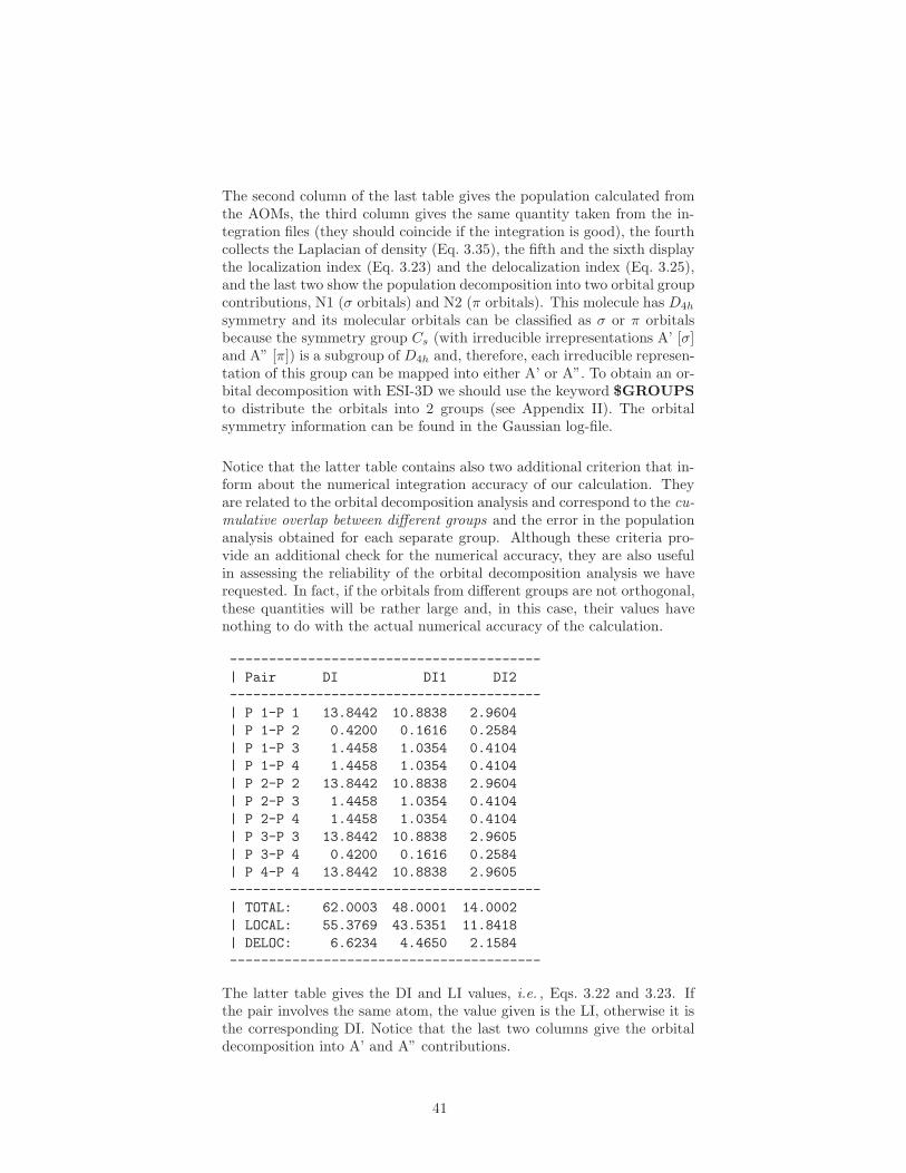
The second column of the last table gives the population calculated fromthe AOMs, the third column gives the same quantity taken from the in-tegration files (they should coincide if the integration is good), the fourthcollects the Laplacian of density (Eq. 3.35), the fifth and the sixth displaythe localization index (Eq. 3.23) and the delocalization index (Eq. 3.25),and the last two show the population decomposition into two orbital groupcontributions, N1 (σ orbitals) and N2 (π orbitals). This molecule has D4h

symmetry and its molecular orbitals can be classified as σ or π orbitalsbecause the symmetry group Cs (with irreducible irrepresentations A’ [σ]and A” [π]) is a subgroup of D4h and, therefore, each irreducible represen-tation of this group can be mapped into either A’ or A”. To obtain an or-bital decomposition with ESI-3D we should use the keyword $GROUPSto distribute the orbitals into 2 groups (see Appendix II). The orbitalsymmetry information can be found in the Gaussian log-file.

Notice that the latter table contains also two additional criterion that in-form about the numerical integration accuracy of our calculation. Theyare related to the orbital decomposition analysis and correspond to the cu-mulative overlap between different groups and the error in the populationanalysis obtained for each separate group. Although these criteria pro-vide an additional check for the numerical accuracy, they are also usefulin assessing the reliability of the orbital decomposition analysis we haverequested. In fact, if the orbitals from different groups are not orthogonal,these quantities will be rather large and, in this case, their values havenothing to do with the actual numerical accuracy of the calculation.

----------------------------------------

| Pair DI DI1 DI2

----------------------------------------

| P 1-P 1 13.8442 10.8838 2.9604

| P 1-P 2 0.4200 0.1616 0.2584

| P 1-P 3 1.4458 1.0354 0.4104

| P 1-P 4 1.4458 1.0354 0.4104

| P 2-P 2 13.8442 10.8838 2.9604

| P 2-P 3 1.4458 1.0354 0.4104

| P 2-P 4 1.4458 1.0354 0.4104

| P 3-P 3 13.8442 10.8838 2.9605

| P 3-P 4 0.4200 0.1616 0.2584

| P 4-P 4 13.8442 10.8838 2.9605

----------------------------------------

| TOTAL: 62.0003 48.0001 14.0002

| LOCAL: 55.3769 43.5351 11.8418

| DELOC: 6.6234 4.4650 2.1584

----------------------------------------

The latter table gives the DI and LI values, i.e. , Eqs. 3.22 and 3.23. Ifthe pair involves the same atom, the value given is the LI, otherwise it isthe corresponding DI. Notice that the last two columns give the orbitaldecomposition into A’ and A” contributions.

41

Finally, we request a multicenter analysis by including the following linesin the input file (either yourfile.fuz or yourfile.bad):

$MULTICENTER

2

4 1 2 3 4

3 1 2 3

Please notice that the atoms should be given in the order they are con-nected in the ring. In these previous lines we request a calculation of twomulticenter indices (P-P-P-P and P-P-P) and ESI produces this result:

----------------------------------------

| Multicenter:

| Atom-Group Iring-like MCI-like

| P 1-P 2-P 3-P 4 = 0.030946 0.069040

| P 1-P 2-P 3 = 0.016717 0.016717

-------------------------------------------

which gives the Iring value, Eq. 3.31, and MCI, Eq. 4.8.

42

Chapter 4

Aromaticity

Chemistry is essentially an experimental science that evolved through experi-mentation and it has been built upon a series of empirically proved laws andmodels. On the other side, quantum mechanics relies on postulates from whicha solid theory has been constructed. Both focus on the study of matter, how-ever, quantum mechanics can anticipate the electronic structure of matter andit could, in principle, replace the laws and models of chemistry by physicallysound theories. Notwithstanding, after many years of the advent of quantummechanics, several chemical concepts with high predictable power still prevail.Most of these concepts have not found (and most likely cannot find) a solid rootin the quantum theory because there is no observable behind them. One findsmany such concepts in the literature (e.g. , chemical bonding, bond order, ionic-ity, electron population, agostic bond, etc.) that are still widely used to predictor explain the electronic structure of molecules or reaction mechanisms. [87] Oneof the most employed terms in literature —and one of the most controversial [88]

ones— is aromaticity. [89–93] Aromaticity is associated with cyclic electron delo-calization in closed circuits giving rise to energy stabilization, bond length equal-ization, large magnetic anisotropies and abnormal chemical shifts, among othereffects. Various of these aromaticity manifestations can be measured by appro-priate quantities, the aromaticity indices, that allow for aromaticity scales. Asa result, nowadays there is a number of indices available in the literature, oftenoffering disparate results about the aromaticity of certain chemical species. [94]

The discovery of new aromatic species [95–97] that extend well beyond the realmof organic chemistry has challenged our understanding of aromaticity and hasput forward limitations of the aromaticity indices to deal with these new chem-ical creatures. [85]

Indeed, aromaticity is an ill-defined concept. It does not correspond to aphysical observable like many other properties that populate the world of toolsused in the routine analysis of chemical reactions. Bond orders, reaction con-certedness or oxidation states are properties that cannot be measured directlyand unambiguously assigned. However, aromaticity is still more controvertedthan other similar quantities like bond ionicity or bond order because it refersnot to one, but several properties that are not necessarily mutually related. De-spite its fuzziness, chemists still use this concept to elucidate phenomena suchas chemical stability/reactivity, bond length equalization/alternation, among

43

others. [90–93] Hence, aromaticity is a concept used by chemists world wide andit cannot be so easily ignored or put aside.

Aromaticity is a multifold property [94,98–101] because its different manifes-tions range from purely energetical to structural ones. The use of different aro-maticity measures (even if they are based on the same manifestation) is highlyrecommended because, as it has been recently proved, [83,102] no aromaticityindex is infallible. On the other hand, saying that aromaticity is a multidi-mensional phenomenon (an accepted fact), sometimes hinders the drawbacksof certain aromaticity indices, which fail to meet results that we would expectfrom chemical grounds. [102] These drawbacks should be identified and the lim-its and features of aromaticity indices stablished to avoid wrong application ofthese quantities. First of all, we should ask ourselves which manisfestation ofaromaticity we are looking for. Aromaticity criteria based on electron delo-calization are good to identify conjugated-electron circuits, which might playimportant roles in the electronic distribution of the electrons in a ring, the mo-bility of the electron cloud or the assignment of electronic spectrum transitions.On the other hand, energetic criteria are important to identify molecules thatbenefit from extra energy stabilization. In some molecules, conjugated-electroncircuits along a ring structure cause bond-length and bond-order equalizationas well as an important energy stabilization in the molecule (many organicmolecules show this behavior). However, the transition state of the Diels-Alderreaction is the most aromatic point along the intrisic reaction coordinate (IRC)but there is no bond-length or bond-order equalization and this point is themost energetic point along the IRC. [103]a

Despite the drastic approximations inherent in the Huckel Molecular Or-bital (HMO) approach, organic aromatic molecules are usually well describedwithin the HMO method. It is thus usual to learn the HMO at the sametime than 4n + 2 Huckel’s rule and other aromaticity measures given by theHMO method, such as the resonance energy (RE), the RE per electron (REPE)or even the topological REPE (TREPE) [106]. Since the studies of Huckel onorganic molecules, the concept of aromaticity has extended importantly in-cluding all sort of new aromatic molecules such as metalloaromatic molecules,fullerens, [107] nanotubes, [108], porphyrins [109,110] molecules with a Mobius-likestructure [111–113] and all-metal clusters, [85] among others.

In the literature there are many indices of aromaticity and they can beclassified as energetic, [114] magnetic [91] geometric [92] and electronic indices, [93]

corresponding to the different manifestations of aromaticity, i.e., energetic sta-bilization, exalted magnetic suceptibilities, [115] particular geometrical features(such as bond length equalization or planarity) or electron delocalization alongthe aromatic ring, respectively. There are various energetic criteria to assessaromaticity but perhaps the most popular one is the use of homodesmotic orisodesmotic reactions from which one can calculate the aromatic stabilizationenergy (ASE). [114] Among the structural-based (or geometric) indices it is worthto highlight the HOMA index. The most popular index of aromaticity is per-

aOne could argue that the energy stabilization should be compared with the transition stateof similar reactions. Yet, pseudopericyclic reactions are essentially barrierless and producesimilar products through a non-aromatic transition state. [104,105]

44

haps the NICS index, [116] which belongs to the set of magnetic indices. Finally,among the electronic indices we find the multicenter indices (Iring and MCI),which perform the best among the different aromaticity indices existing in theliterature. [83,102]

In this course we will mostly focus on the study of a geometric index ofaromaticity (HOMA), [117] a magnetic one (NICS) [116] and several electronic in-dices of aromaticity, which include FLU, [118] Iring , [76] MCI [77] and PDI. [119]

4.1 Global and Local Aromaticity

Several manifestations of aromaticity are related to the whole molecular struc-ture, whereas others are specific of a given annular structure within the molecule.The former are known as global properties and the latter concern only specific re-gions of the molecule and, therefore, are local properties of the molecule. Globalaromaticity indicators include the HOMO-LUMO gap (or simply energy gap)that is directly related with the ability of the molecule to undergo chemicalreactions. The larger the gap, the least (energetically) accessible the LUMOorbital is and, thus, the least reactive the molecule is expected to be. Thisextra energy stabilization is characteristic of aromatic molecules. On the otherhand, geometrical features (bond length equalization or bond distances halfwaybetween single and double bonds), electronic ring currents (induced by an ex-ternal magnetic field perpendicular to the ring plane) or multicenter electronicdelocalization along the atoms in the ring are typical characteristics of annu-lar structures within the the molecule and are regarded as local aromaticityfeatures.

In the following section we will study several aromaticity indices. In the caseof local aromaticity indices we will assume a molecule having at least one ringstructure, which consists of n atoms represented by the string A=A1,A2,...,An,whose elements are ordered according to the connectivity of the atoms in thering. For convenience, we adopt An+1 ≡ A1.

4.2 Geometrical indices

In this subsection we will analyze the so-called harmonic oscilator model ofaromaticity (HOMA) as defined by Kruszewski and Krygowski. [117] The HOMAonly relies on geometrical data and it can be computed using this expression:b

HOMA(A) = 1 − 257.71

n

n∑

i

(

Ropt −RAi,Ai+1

)2(4.1)

= 1 − 257.7

(

(

Ropt −R)2

+1

n

n∑

i

(

RAi,Ai+1−R

)2

)

(4.2)

= 1 − (EN + GEO) (4.3)

bPlease notice that the step from Eq. 4.1 to Eq. 4.2 assumes that all bonds are of the sametype. The expression for rings with different bonding patterns can also be decomposed intoEN and GEO terms but its derivation is less straightforward. [120]

45

where the reference bond lengths, Ropt, are chosen so that the compression en-ergy of the double bond and expansion energy of the single bond are minimalaccording to the harmonic potential model. The closer to one the index, themore aromatic the molecule. The formula depends on some reference bond dis-tances and, unfortunately, there is a limited number of bonds for which thesereferences have been tabulated (C-C, C-N, C-O, C-P, C-S, N-N and N-O). Thisset suffices to calculate most organic molecules but imposes a serious drawbackto extend the use of HOMA to new aromatic molecules.

The EN component of HOMA measures the deviation of the interatomic dis-tances as compared to some tabulated numbers. GEO measures the variance ofthe interatomic distance, which for aromatic molecules is usually a small num-ber because, unlike antiaromatic molecules, aromatic molecules do not presentbond-length alternation (BLA). Both quantities, EN and GEO, are close to zerofor aromatic molecules.

Another popular geometrical indicator of aromaticity is the BLA, whichcompares the average of bond-lengths of consecutive bonds in a ring:

BLA (A) =1

n1

n1∑

i=1

rA2i−1,A2i−

1

n2

n2∑

i=1

rA2i,A2i+1(4.4)

where n1 = ⌊(n+ 1) /2⌋ and n2 = ⌊n/2⌋, ⌊x⌋ being the floor function of x, thatreturns the largest integer less than or equal to x.

4.3 Magnetic indices

If an aromatic molecule is exposed to an external magnetic field, this field in-duces a π-electron ring current that can be measured and used to character-ize aromaticity. The magnetic susceptibility exaltation or the anisotropy ofthe magnetic susceptibility are measures of aromaticity based on this property.However, the most important (and by far the most popular) magnetic index ofaromaticity is the nucleus independent chemical shift (NICS). The NICS is thenegative value of the absolute shielding computed at the center of the ring (orother relevant point of the system, see below). It was defined by Paul Schleyerand coworkers [116] and predicts that the most aromatic molecules will be thosewith the most negative values. On the contrary, the more positive the NICSvalues, the more antiaromatic the rings are.

There are many NICS variants; NICS can be calculated at the ring center[NICS(0)], at one Angstrom above or below the ring plane [NICS(1)]c or takingonly its out-of-plane tensor component [NICS(0)zzand NICS(1)zz ]. Finally, itis worth saying that some authors recommend to compute the NICS not at thegeometric center but at the point of the lowest density in the ring plane, i.e., atthe RCP. [121] This recommendation is particularly wise in the case of hetero-cyclic or metalloaromatic compounds, where the RCP is usually displaced from

cThe NICS(1) should in principle capture the presence of π-electron delocalization becausethe maximum of the p orbital occurs at ca. 1A. NICS(1) is thus more suitable for organicmolecules, which exhibit classical π aromaticity.

46

the geometric ring center.

Finally, it is worth mentioning that several authors have suggested using theprofile of NICS obtained by a NICS scan along the line perpendicular to themolecular plane or within the molecular plane. [84,122,123]

4.4 Electronic indices

Despite aromaticity does not accept a unique definition, there has been manyattempts to define it. Perhaps the most remarkable ones are due to Sondheimer(1963) and Paul Schleyer (1996) in two articles from the official journal of theInternational Union of Pure and Applied Chemistry (IUPAC): [89,124]

A compound is considered to be aromatic if there is a measurabledegree of delocalization of a π-electron system in the ground state ofthe molecule.

F. Sondheimer (1963)

Aromaticity is now associated with cyclic arrays of mobile elec-trons with favorable symmetries. In contrast, the unfavorable sym-metry properties of antiaromatic systems lead to localized, ratherthan to delocalized electronic structures. The ”mobile electron” ar-rays are not restricted to π, but may be σ or mixed in character.

P. Schleyer and H. Jiao (1996)

Sondheimer considers aromatic molecules as those that have a measurable de-gree of cyclic delocalization of a π-electron system. Similarly, Schleyer and Jiaothink of aromaticity as associated with cyclic arrays of mobile electrons with fa-vorable symmetries while the unfavorable symmetry properties of antiaromaticsystems leads to localized rather than to delocalized electronic structures. Thiscyclic mobility of electrons is translated into characteristic aromatic manifes-tations such as bond-length equalization, abnormal chemical shifts, magneticanisotropies, and energetic stabilization.

It is thus only natural to define aromaticity from its source characteristic, theparticular electronic distribution, rather than from its consequences. Lately aro-maticity indicators based on the electronic structure of molecules are becomingpopular, and several research groups have designed new aromaticity indices. [93]

Among others we can mention the Iring[76] of Giambiagi et al., the MCI [77] of

Bultinck and coworkers, the θ index [125] of Matta or the Shannon Entropy atthe BCP as suggested by Noorizadeh et al. [126] More recently, Szczepanik andcoworkers have contributed with a index capable of accounting for multicenterbonding. [127,128] Our group has been also extensively working in this issue [90,93],and the latest efforts have provided the PDI [119] and FLU [118] aromaticity mea-sures as well as the normalized versions of Iring and MCI. [78] Lately AV1245 [129]

and AVmin, [130,131] which are aromaticity index for large rings, have been de-fined.

47

Some aromaticity indices have been proposed based only on the fact thatthey provide a good correlation with previously reported aromaticity indices.It is thus recommended to know the limitations of the existing aromaticityindices and some of them can only be learned by experience. [83,102] In the nextsubsection we will give the definitions and analyze the features of a few electronicaromaticity indices.

4.4.1 The Aromatic Fluctuation Index: FLU

The FLU index measures aromaticity by comparison with cyclic electron delo-calization in typical aromatic molecules, [118,132]

FLU(A) =1

n

n∑

i=1

[(

δ(Ai)

δ(Ai−1)

)α(δ(Ai, Ai−1) − δref (Ai, Ai−1)

δref (Ai, Ai−1)

)]2

, (4.5)

where A0 ≡ An and δ(A) is the atomic valence for a closed-shell system,Eq. 3.25, and α is a simple function to ensure the first term in Eq. (4.5) isalways greater or equal to 1,

α =

1 δ(Ai−1) ≤ δ(Ai)

−1 δ(Ai) < δ(Ai−1)(4.6)

δ(A,B) and δref (A,B) are DI (see Eq. 3.22), i.e. quantities that account forthe electron sharing of A and B, the latter DI corresponding to an aromaticmolecule which has the pattern of bonding A−B. The aromatic references forC-C bonds is benzene, whereas C-N bond references are taken from pyridine.FLU is close to zero in aromatic species, and greater than zero in non-aromaticor antiaromatic species.

The aromaticity indices based on references do not actually measure aro-maticity but they measure the similarity with respect to some aromatic molecule.In this sense, HOMA and FLU are not adequate to describe reactivity. Forinstance, in the case of the Diels-Alder reaction they cannot recognize the tran-sition state (TS) as the most aromatic point along the reaction path becausethe product, cyclohexene, is more similar to benzene (the reference molecule forC-C bonds) than the TS, which shows large C-C distances and small DIs in thebonds that will be formed. [103]

4.4.2 A Multicenter based index: Iring

Giambiagi and coworkers suggested to use the multicenter index (which accountsfor the simultaneous electron sharing among various centers) as a measure ofaromaticity. The index was name Iring and its formulation was given in Eq. 3.31.The formulation for single-determinant wavefunctions applied into a ring struc-ture, A, reads as follows [76]:

Iring(A) =

occ∑

i1,i2,...,in

Si1i2(A1)Si2i3(A2)...Sini1(An) (4.7)

48

where Sij(A) is the overlap of molecular orbitals i and j in the atom A (seeEq. 3.22). Iring will provide large values (larger simultaneous electron sharingof atoms in the ring) for aromatic molecules.

4.4.3 The Multicenter Index: MCI

With the aim to improve the Iring , Bultinck and coworkers [77] proposed tosum not only the contribution from the Kekule structures (as Iring does), butalso the contributions of all structures generated by permuting the position ofall the atoms in the ring. Such possibility was already discussed by Ponec andcowokers [71,133] among others [134]. The index was named MCI and its expressionis as follows:

MCI(A) =∑

P(A)

Iring(A) (4.8)

=∑

P(A)

occ∑

i1,i2,...,in

Si1i2(A1)Si2i3(A2)...Sini1 (An) (4.9)

where P(A) stands for n! permutations of elements in the string A. Althoughthe original proposal of MCI differs from this one by a numerical factor, we willskip it for the reasons already commented in ref. [78]. Like Iring , MCI produceslarge numbers for aromatic species, and the authors claim negative numbersidentify antiaromatic species. [135] To my knowledge, this fact has only beenproven for three-member rings [71] and heuristically for six-member rings. [136]

4.4.4 The para-Delocalization Index: PDI

Fulton [137] and Bader [138] showed that benzene has larger DI between the atomsin para position than in meta position. This finding was used by Poater et al. [119]

to define the para-delocalization index (PDI), which consists in the average DIbetween atoms in para position in a six-membered ring,

PDI(A) =δ(A1, A4) + δ(A2, A5) + δ(A3, A6)

3. (4.10)

The larger the index, the greater the aromaticity. Obviously, the index cannotbe applied to rings with more or less than six members. The PDI is less realiablefor heterocycles and rings made of highly polarizable atoms [102] because it canincrease the delocalization across the ring without a substantial increase of theperipheral delocalization.

4.4.5 The Bond-Order Alternation

The BLA is built upon the premise that the bond-length alternation (i.e. , ageometrical feature) reflects the distribution of electron pairs on a conjugatedcircuit. For this reason, some people prefer an electronic-structure formulationequivalent of the BLA, the bond-order alternation (BOA), which uses the bond

49

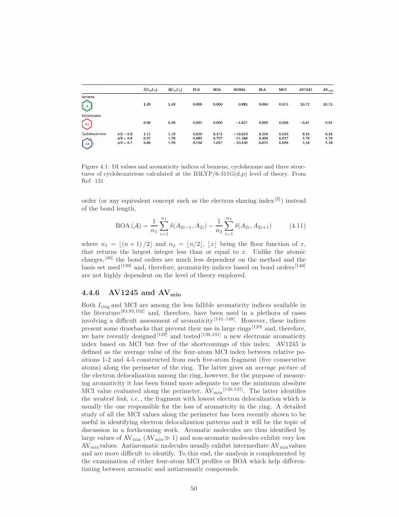
Figure 4.1: DI values and aromaticity indices of benzene, cyclohexane and three struc-tures of cyclohexatriene calculated at the B3LYP/6-311G(d,p) level of theory. FromRef. 131

order (or any equivalent concept such as the electron sharing index [2]) insteadof the bond length,

BOA (A) =1

n1

n1∑

i=1

δ(A2i−1, A2i) −1

n2

n2∑

i=1

δ(A2i, A2i+1) (4.11)

where n1 = ⌊(n+ 1) /2⌋ and n2 = ⌊n/2⌋, ⌊x⌋ being the floor function of x,that returns the largest integer less than or equal to x. Unlike the atomiccharges, [46] the bond orders are much less dependent on the method and thebasis set used [139] and, therefore, aromaticity indices based on bond orders [140]

are not highly dependent on the level of theory employed.

4.4.6 AV1245 and AVmin

Both Iring and MCI are among the less fallible aromaticity indices available inthe literature [83,93,102] and, therefore, have been used in a plethora of casesinvolving a difficult assessment of aromaticity [141–148]. However, these indicespresent some drawbacks that prevent their use in large rings [129] and, therefore,we have recently designed [129] and tested [130,131] a new electronic aromaticityindex based on MCI but free of the shortcomings of this index. AV1245 isdefined as the average value of the four-atom MCI index between relative po-sitions 1-2 and 4-5 constructed from each five-atom fragment (five consecutiveatoms) along the perimeter of the ring. The latter gives an average picture ofthe electron delocalization among the ring, however, for the purpose of measur-ing aromaticity it has been found more adequate to use the minimum absoluteMCI value evaluated along the perimeter, AVmin

[130,131]. The latter identifiesthe weakest link, i.e. , the fragment with lowest electron delocalization which isusually the one responsible for the loss of aromaticity in the ring. A detailedstudy of all the MCI values along the perimeter has been recently shown to beuseful in identifying electron delocalization patterns and it will be the topic ofdiscussion in a forthcoming work. Aromatic molecules are thus identified bylarge values of AVmin (AVmin≫ 1) and non-aromatic molecules exhibit very lowAVminvalues. Antiaromatic molecules usually exhibit intermediate AVminvaluesand are more difficult to identify. To this end, the analysis is complemented bythe examination of either four-atom MCI profiles or BOA which help differen-tiating between aromatic and antiaromatic compounds.

50

4.4.7 EXERCISE 8 (Aromaticity)

In this exercise we will perform an aromaticity calculation to use all the afore-mentioned indices. We will take two molecules benzene and cyclohexane.

Electronic aromaticity indices. To obtain the electronic aromaticityindices we just need to perform the same steps that we did to calculate theelectronic sharing indices (see exercises 5 and 6) and the output of ESI-3D willinclude all the electronic aromaticity indices for the rings specified by the key-word $RING (see Appendix II).

Keep in mind that FLU uses reference values and it only has values for thebonds C-C, C-N, B-N and N-N, any other bond patterns in the rings cannot becalculated with FLU and should be disregarded. On the other hand, PDI canonly be calculated in six-member rings. MCI and Iring do not have any limita-tion and can be calculated in any molecular ring, the only exception being largeporphyrinc rings. [129]

The input file (benzene.bad) of ESI-3D for benzene molecule looks like this:

$READWFN

benzene.wfn

$RING

1

6

2 1 3 7 10 6

$FULLOUT

The keyword $READWFN specifies the wfn-file generated by AIMall. Thekeyword $RING is used to specify the ring structure (1 ring, 6 members in thisring, which are atoms 2 1 3 7 10 and 6). The keyword $FULLOUT is usedto get additional printout containing more information about the indices calcu-lated.

For small molecules the ESI-3D program can be executed without submit-ting the job into the queue,

/users/eduard/QUANT/ESI/ESI benzene.bad > benzene.esi

See below an extract from ESI-3D program (collected in benzene.esi con-cerning the aromaticity calculations of the last molecule:

----------------------------------------------------------------------

| Aromaticity indices - FLU [JCP 122, 014109 (2005)]

| HOMA [Tetrahedron 52, 10255 (1996)]

| PDI [CEJ 9, 400 (2003)]

| Iring [PCCP 2, 3381 (2000)]

| MCI [JPOC 18, 706 (2005)]

| I_NB, I_NG [JPCA 111, 6521 (2007)]

| For a recent review see: [CSR 44, 6434 (2015)]

----------------------------------------------------------------------

51

|

| Ring 1 (6): 2 1 3 7 10 6

|

| No number of pi electrons provided. I take 6.00000

| Atom pair delta i-->j j-->i Exc(i,j) diff Flu(i,j)

----------------------------------------------------------------------

| C 1-C 2 1.38730 0.33755 0.33756 1.00001 -0.00907 0.0000822

| C 1-C 3 1.38735 0.33757 0.33756 1.00001 -0.00903 0.0000816

| C 3-C 7 1.38733 0.33756 0.33756 1.00002 -0.00905 0.0000819

| C 7-C 10 1.38730 0.33756 0.33755 1.00001 -0.00907 0.0000822

| C 6-C 10 1.38735 0.33756 0.33757 1.00001 -0.00903 0.0000816

| C 2-C 6 1.38733 0.33756 0.33756 1.00002 -0.00905 0.0000819

----------------------------------------------------------------------

| FLU 1 = 0.000082

| FLUm 1 = 0.000082

----------------------------------------------------------------------

----------------------------------------------------------------------

| BOA 1 = 0.000000

| BOAvg 1 = 1.387329

| TREPE 1 = 0.045432

----------------------------------------------------------------------

| PDI 1 = 0.103425 ( 0.103427 0.103429 0.103419 )

| ESI will use traditional MCI algorithm

| Iring 1 = 0.048553

| I_NG 1 = 0.041397

| MCI 1 = 0.072991

| I_NB 1 = 0.041177

----------------------------------------------------------------------

In this case FLU is zero (i.e. maximum aromaticity) because the referencemolecule is benzene (FLUm is the maximum value of FLU bond contributions).BOA is zero because there is no bond-order alternation in this molecule. PDIis 0.1, which is quite large value for a para-DI, thus indicating that benzene isaromatic. The output also provides the geometrical center of the ring (in A) sothat we can use this information to calculate NICS(0) on a separate Gaussiancalculation. The multicenter indices, Iring and MCI, show large numbers, 0.049and 0.073, respectively. I NG (normalized version of Iring , see Ref.) [78] andI NB (normalized version of MCI, see also Ref.) [78] show also large numberstypical of aromatic molecules. For comparison we add below the extract ofcyclohexane:

----------------------------------------------------------------------

| FLU 1 = 0.095695

| FLUm 1 = 0.095731

----------------------------------------------------------------------

----------------------------------------------------------------------

| BOA 1 = 0.000001

| TREPE 1 = 0.045432

----------------------------------------------------------------------

| PDI 1 = 0.008517 ( 0.008523 0.008546 0.008482 )

| Iring 1 = 0.000286

52

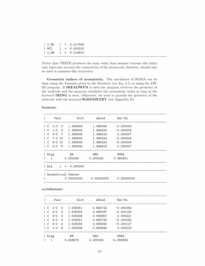
| I_NG 1 = 0.017594

| MCI 1 = 0.000315

| I_NB 1 = 0.016610

----------------------------------------------------------------------

Notice that TREPE produces the same value than benzene because this indexonly takes into account the connectivity of the atoms and, therefore, should onlybe used in annulene-like structures.

Geometric indices of aromaticity. The calculation of HOMA can bedone using the formulae given in the literature (see Eq. 4.1) or using the ESI-3D program. If $READWFN is used the program retrieves the geometry ofthe molecule and the program calculates the aromaticity index as long as thekeyword $RING is used. Otherwise, we need to provide the geometry of themolecule with the keyword $GEOMETRY (see Appendix II).

benzene:

----------------------------------------------------------------------

| Pair Dist nBond Rav-Ri

----------------------------------------------------------------------

| C 1-C 2 1.399549 1.486324 -0.000004

| C 1-C 3 1.399549 1.486324 -0.000004

| C 3-C 7 1.399538 1.486418 0.000007

| C 7-C 10 1.399549 1.486324 -0.000004

| C 6-C 10 1.399549 1.486324 -0.000004

| C 2-C 6 1.399538 1.486418 0.000007

----------------------------------------------------------------------

| Ring EN GEO HOMA

| 1 0.034349 0.000000 0.965651

----------------------------------------------------------------------

| BLA 1 = 0.000000

----------------------------------------------------------------------

| Geometrical Center:

| 0.00000000 0.00000000 0.00000000

----------------------------------------------------------------------

cyclohexane:

----------------------------------------------------------------------

| Pair Dist nBond Rav-Ri

----------------------------------------------------------------------

| C 1-C 2 1.536251 0.665722 -0.000094

| C 2-C 3 1.536284 0.665597 -0.000126

| C 3-C 4 1.535936 0.666957 0.000221

| C 4-C 5 1.536251 0.665726 -0.000093

| C 5-C 6 1.536285 0.665592 -0.000127

| C 1-C 6 1.535938 0.666948 0.000219

----------------------------------------------------------------------

| Ring EN GEO HOMA

| 1 5.656675 0.000006 -4.656682

53

----------------------------------------------------------------------

| BLA 1 = 0.000000

----------------------------------------------------------------------

| Geometrical Center:

| 0.00000027 0.00000008 -0.00000015

----------------------------------------------------------------------

HOMA=0.97 for benzene, which is very close to the maximum value. Thesmall deviation is due to the EN component, as all the bonds are equivalent and,therefore, GEO=0 and BLA=0. On the other hand, cyclohexane value is muchsmaller than zero, indicating that this molecule is not aromatic at all. The ge-ometrical criteria, GEO, (which measures the deviation from the average bonddistance in the ring) is zero for both molecules, indicating that all the bondshave the same length and, therefore, as far as the symmetry is concerned, themolecules should be very aromatic because there is no bond length alternation(BLA=0). On the other hand, EN is also close to zero in benzene because allthe C-C are, obviously, very close to the optimal C-C distance, whereas cyclo-hexane gives a very large EN value, in accord to the C-C distances which arelarger than typical aromatic molecule.

Magnetic indices of aromaticity. The calculation of NICS has to bedone with gaussian by requesting an NMR calculation (keyword to add in theinput file: NMR) and including a list of the relevant points that we want tospecify as Bq. See this example for benzene:

#HF/6-31G* NMR

NICS automatic generation

0 1

C 0.00000000 1.38617405 0.00000000

C 1.20046194 0.69308703 0.00000000

C 1.20046194 -0.69308703 0.00000000

C 0.00000000 -1.38617405 0.00000000

C -1.20046194 -0.69308703 0.00000000

C -1.20046194 0.69308703 0.00000000

H 0.00000000 -2.46178023 0.00000000

H 2.13196422 -1.23089011 0.00000000

H 2.13196422 1.23089011 0.00000000

H 0.00000000 2.46178023 0.00000000

H -2.13196422 1.23089011 0.00000000

H -2.13196422 -1.23089011 0.00000000

Bq 0.00000000 0.00000000 0.00000000

Bq 0.00000000 0.00000000 1.00000000

Bq 0.00000000 0.00000000 -1.00000000

In this case, benzene is placed in the σXY plane and the NICS(0) point is lo-cated at (0,0,0). NICS(1) is calculated by placing Bq(s) at (0,0,-1) and (0,0,1).In case your molecule is not symmetric, you should identify the σ plane thatcontains the atoms of the target ring. Either you calculate σ from the geometry

54

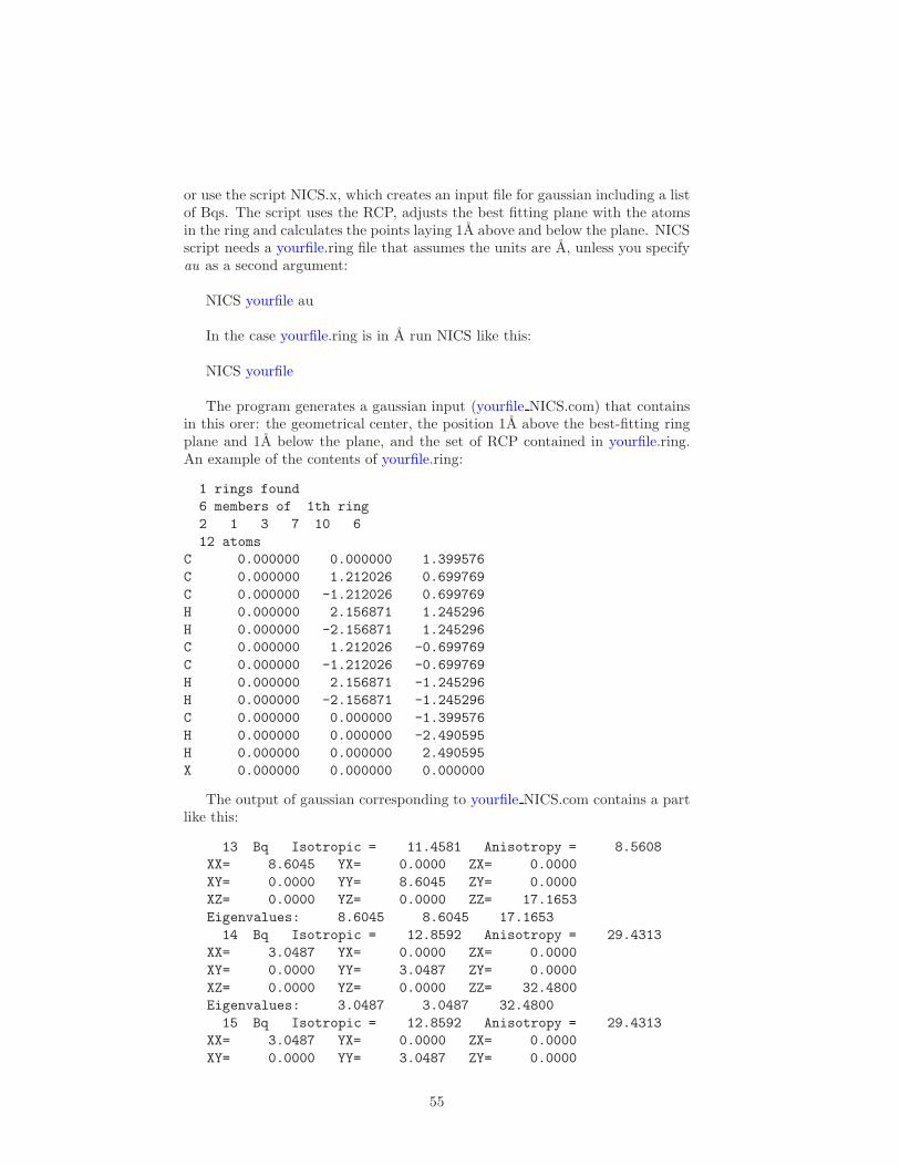
or use the script NICS.x, which creates an input file for gaussian including a listof Bqs. The script uses the RCP, adjusts the best fitting plane with the atomsin the ring and calculates the points laying 1A above and below the plane. NICSscript needs a yourfile.ring file that assumes the units are A, unless you specifyau as a second argument:

NICS yourfile au

In the case yourfile.ring is in A run NICS like this:

NICS yourfile

The program generates a gaussian input (yourfile NICS.com) that containsin this orer: the geometrical center, the position 1A above the best-fitting ringplane and 1A below the plane, and the set of RCP contained in yourfile.ring.An example of the contents of yourfile.ring:

1 rings found

6 members of 1th ring

2 1 3 7 10 6

12 atoms

C 0.000000 0.000000 1.399576

C 0.000000 1.212026 0.699769

C 0.000000 -1.212026 0.699769

H 0.000000 2.156871 1.245296

H 0.000000 -2.156871 1.245296

C 0.000000 1.212026 -0.699769

C 0.000000 -1.212026 -0.699769

H 0.000000 2.156871 -1.245296

H 0.000000 -2.156871 -1.245296

C 0.000000 0.000000 -1.399576

H 0.000000 0.000000 -2.490595

H 0.000000 0.000000 2.490595

X 0.000000 0.000000 0.000000

The output of gaussian corresponding to yourfile NICS.com contains a partlike this:

13 Bq Isotropic = 11.4581 Anisotropy = 8.5608

XX= 8.6045 YX= 0.0000 ZX= 0.0000

XY= 0.0000 YY= 8.6045 ZY= 0.0000

XZ= 0.0000 YZ= 0.0000 ZZ= 17.1653

Eigenvalues: 8.6045 8.6045 17.1653

14 Bq Isotropic = 12.8592 Anisotropy = 29.4313

XX= 3.0487 YX= 0.0000 ZX= 0.0000

XY= 0.0000 YY= 3.0487 ZY= 0.0000

XZ= 0.0000 YZ= 0.0000 ZZ= 32.4800

Eigenvalues: 3.0487 3.0487 32.4800

15 Bq Isotropic = 12.8592 Anisotropy = 29.4313

XX= 3.0487 YX= 0.0000 ZX= 0.0000

XY= 0.0000 YY= 3.0487 ZY= 0.0000

55

XZ= 0.0000 YZ= 0.0000 ZZ= 32.4800

We must take the negative value of the Isotropic contribution. Therefore, inthis case NICS(0)=-11.5,d NICS(0)zz=-17.2, NICS(1)=-12.9 and NICS(1)zz=-32.5. All the values indicate that benzene is an aromatic molecule, the impor-tant values in this case are the total, NICS(1), and perpendicular component,NICS(1)zz , that indicate the aromaticity of benzene is due to the π-electrondelocalization along the ring.

dThe isotropic NICS(0) values is obtained as an average of NICS(0)xx , NICS(0)yy andNICS(0)zz .

56

Chapter 5

Oxidation state

5.1 Definition

Historically, the oxidation state (OS) was defined as the stepwise increase in theamount of oxygen bound by atoms that form more than one oxide. Nowadays,the concept of OS is mostly used for transition metal (TM) complexes and,therefore, the interest on calculating OS is focused on TM atoms. Figure ??summarizes the OS of the first three rows of TM elements.

The OS is a property of an atom within a molecule. As such, its definition isnot completely unambiguous and there is a number of cases where the oxidationstate cannot be clearly assigned. [149] There are complicated bonding situationsinvolving noninnocent ligands or intermediates or transition states of reactions,where the formal OS assignment might be rather ambiguous. Therefore, it isimportant to have realiable methods to assign oxidation states in troublesomecases.

The IUPAC defined the OS as the charge of the central atom (often a TM)after removing its neighbors (the ligands) along with the shared electron pairs.There are a number of papers published by the IUPAC about the OS, but letus consider here the extensive report of Pavel Karen published in 2014. [149] For

Figure 5.1: The common oxidation states of the first three rows of TM atoms in theperiodic table.

57

Figure 5.2: The interaction of Fe4+ with PhO− can give rise to two oxidation states. Ifwe consider the formal oxidation state, the OS of Fe is IV, whereas the spectroscopicmeasurements indicate that Fe only populates d orbitals with 4 electrons, i.e. , the OSof Fe is III.

a short account of the OS and its state-of-the-art calculation see the essay bythe same author, Ref. 150

There have been attempts to define the OS in a less ambiguous way. Forinstance, the physical or spectroscopic OS is the charge of the TM thatcomes from dn and can be measured spectroscopically (e.g. from Mossbauer).a

Figure 5.2 illustrates one of the few examples where the formal definition of OSstates differs from the spectroscopic one.

5.2 Computational calculation of Oxidation States

There are many methods to calculate the OS, for a historical account seeRef. [149] and for a short list see Ref.) [150] (see also Refs. [151,152]. Here we willconsider only a few approches: the empirical approach based on metal-to-liganddistance, the bond valence sum, and three different computational approaches:the population analysis, the spin density and orbital-localization methods.

In order to perform a comparison between the different methods to calculateoxidation states we have chosen a set of TM complexes, taken from Ref.; [151]

these TM complexes and the oxidation state of its central atom are collected inTable 5.1.

5.2.1 Bond Valence Sum

The Bond Valence Sum (BVS) method is an empirical technique based on themetal-to-ligand distances (Ri) and some reference values (R0, b=0.37A).b TheBVS expression reads:

V =∑

i

(

Ri −R0

b

)

aJorgensen, In Oxidation Numbers and Oxidation States; Springer; Heildeberg, 1969.Useful references:http://www.edu.upmc.fr/chimie/mc741/PDFs/bond.pdfhttp://www.chem.umn.edu/groups/harned/classes/8322/lectures/5ElectronCounting.pdf

bhttp://www.ccp14.ac.uk/solution/bond valence/index.html

58

VII [V Cl6]4− [V (H2O)6]

2+ [V (CN)6]4− [V (CO)6]

2+

MnII [MnCl6]4− [Mn(H2O)6]

2+ [Mn(CN)6]4− [Mn(CO)6]

2+

MnIII [MnCl6]3− [Mn(H2O)6]

3+ [Mn(CN)6]3− [Mn(CO)6]

3+

FeII [FeCl6]4− [Fe(H2O)6]

2+ [Fe(CN)6]4− [Fe(CO)6]

2+

FeIII [FeCl6]3− [Fe(H2O)6]

3+ [Fe(CN)6]3− [Fe(CO)6]

3+

NiII [NiCl6]4− [Ni(H2O)6]

2+ [Ni(CN)6]4− [Ni(CO)6]

2+

ZnII [ZnCl6]4− [Zn(H2O)6]

2+ [Zn(CN)6]4− [Zn(CO)6]

2+

Table 5.1: The set of TM complexes from Ref.. [151]

This method only needs the computational optimization of the TM complexgeometry.

5.2.2 Atom Population Analysis

In section 3.6, we studied different methods to calculate atomic populations.In order to state the OS from atomic populations, we simply need to takethe closest integer number to the atomic charge, Eq. 3.14. Although it is acommon practice in the literature to estimate the OS from atomic populations,the method is perhaps the least reliable one. The atomic populations havea strong dependency on the method used to perform the atomic partition. [46]

Besides, some atomic partitions, such as Mulliken’s (see section 3.6.1) show astrong basis set dependency. In Table 5.2 we collect the OS of the set of TMcomplexes calculated with Mulliken and TFVC partitions. Mulliken populationfails in all cases but TFVC fails more than 50% of the tests. [153]

Cl− H2OHS H2O

LS CN− CO Cl− H2OHS H2O

LS CN− CO

VII 0.98 1.12 0.05 0.64 1.60 1.76 - 1.60 1.64MnII 1.10 1.24 1.18 0.10 0.64 1.36 1.64 1.70 1.53 1.53MnIII 0.93 1.58 1.52 0.35 0.80 1.46 2.05 2.09 1.58 1.67

FeII 0.86 1.22 1.15 0.01 0.51 1.27 1.63 1.77 1.46 1.44FeIII 0.99 1.64 1.48 0.24 0.66 1.44 2.06 1.98 1.49 1.58NiII 0.99 1.08 -0.19 0.31 1.27 - 1.59 1.24 1.30ZnII 1.02 1.06 -0.03 0.52 1.25 - 1.45 1.15 1.19

Table 5.2: The OS for set of TM complexes from Ref.. [151] The values on the l.h.s.correspond to Mulliken charges and the ones in the r.h.s. to TFVC, from Ref.. [153]

The values marked in green are correctly predicted.

5.2.3 Spin Densities

Crystal Field Theory (CFT) is a model that describes the breaking of degen-eracies of electron orbital states, usually d or f orbitals, due to a static electricfield produced by a surrounding charge distribution (neighboring anions). TheCFT can be used in conjunction with the field strength of the complex ligandsto predict the occupation of the d orbitals in the TM. From this occupationone can infer the number of unpaired electrons in the TM for each possible

59

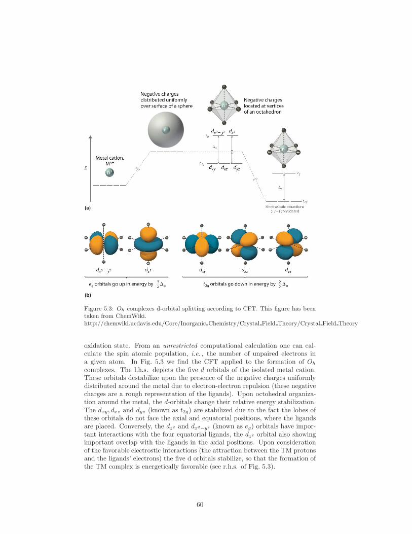
Figure 5.3: Oh complexes d-orbital splitting according to CFT. This figure has beentaken from ChemWiki.http://chemwiki.ucdavis.edu/Core/Inorganic Chemistry/Crystal Field Theory/Crystal Field Theory

oxidation state. From an unrestricted computational calculation one can cal-culate the spin atomic population, i.e. , the number of unpaired electrons ina given atom. In Fig. 5.3 we find the CFT applied to the formation of Oh

complexes. The l.h.s. depicts the five d orbitals of the isolated metal cation.These orbitals destabilize upon the presence of the negative charges uniformlydistributed around the metal due to electron-electron repulsion (these negativecharges are a rough representation of the ligands). Upon octohedral organiza-tion around the metal, the d-orbitals change their relative energy stabilization.The dxy, dxz and dyz (known as t2g) are stabilized due to the fact the lobes ofthese orbitals do not face the axial and equatorial positions, where the ligandsare placed. Conversely, the dz2 and dx2−y2 (known as eg) orbitals have impor-tant interactions with the four equatorial ligands, the dz2 orbital also showingimportant overlap with the ligands in the axial positions. Upon considerationof the favorable electrostic interactions (the attraction between the TM protonsand the ligands’ electrons) the five d orbitals stabilize, so that the formation ofthe TM complex is energetically favorable (see r.h.s. of Fig. 5.3).

60

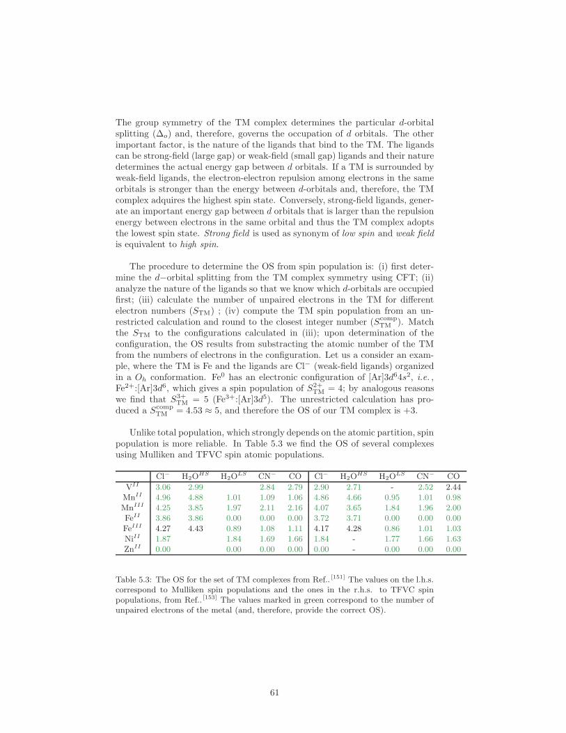
The group symmetry of the TM complex determines the particular d-orbitalsplitting (∆o) and, therefore, governs the occupation of d orbitals. The otherimportant factor, is the nature of the ligands that bind to the TM. The ligandscan be strong-field (large gap) or weak-field (small gap) ligands and their naturedetermines the actual energy gap between d orbitals. If a TM is surrounded byweak-field ligands, the electron-electron repulsion among electrons in the sameorbitals is stronger than the energy between d-orbitals and, therefore, the TMcomplex adquires the highest spin state. Conversely, strong-field ligands, gener-ate an important energy gap between d orbitals that is larger than the repulsionenergy between electrons in the same orbital and thus the TM complex adoptsthe lowest spin state. Strong field is used as synonym of low spin and weak fieldis equivalent to high spin.

The procedure to determine the OS from spin population is: (i) first deter-mine the d−orbital splitting from the TM complex symmetry using CFT; (ii)analyze the nature of the ligands so that we know which d-orbitals are occupiedfirst; (iii) calculate the number of unpaired electrons in the TM for differentelectron numbers (STM) ; (iv) compute the TM spin population from an un-restricted calculation and round to the closest integer number (Scomp

TM ). Matchthe STM to the configurations calculated in (iii); upon determination of theconfiguration, the OS results from substracting the atomic number of the TMfrom the numbers of electrons in the configuration. Let us a consider an exam-ple, where the TM is Fe and the ligands are Cl− (weak-field ligands) organizedin a Oh conformation. Fe0 has an electronic configuration of [Ar]3d64s2, i.e. ,Fe2+:[Ar]3d6, which gives a spin population of S2+

TM = 4; by analogous reasonswe find that S3+

TM = 5 (Fe3+:[Ar]3d5). The unrestricted calculation has pro-duced a Scomp

TM = 4.53 ≈ 5, and therefore the OS of our TM complex is +3.

Unlike total population, which strongly depends on the atomic partition, spinpopulation is more reliable. In Table 5.3 we find the OS of several complexesusing Mulliken and TFVC spin atomic populations.

Cl− H2OHS H2O

LS CN− CO Cl− H2OHS H2O

LS CN− CO

VII 3.06 2.99 2.84 2.79 2.90 2.71 - 2.52 2.44MnII 4.96 4.88 1.01 1.09 1.06 4.86 4.66 0.95 1.01 0.98MnIII 4.25 3.85 1.97 2.11 2.16 4.07 3.65 1.84 1.96 2.00FeII 3.86 3.86 0.00 0.00 0.00 3.72 3.71 0.00 0.00 0.00

FeIII 4.27 4.43 0.89 1.08 1.11 4.17 4.28 0.86 1.01 1.03NiII 1.87 1.84 1.69 1.66 1.84 - 1.77 1.66 1.63ZnII 0.00 0.00 0.00 0.00 0.00 - 0.00 0.00 0.00

Table 5.3: The OS for the set of TM complexes from Ref.. [151] The values on the l.h.s.correspond to Mulliken spin populations and the ones in the r.h.s. to TFVC spinpopulations, from Ref.. [153] The values marked in green correspond to the number ofunpaired electrons of the metal (and, therefore, provide the correct OS).

61

5.2.4 Orbital-localization Methods: Effective OxidationState

We are concerned here with the effective oxidation state (EOS) method ofRamos-Cordoba, Postils and Salvador [152] but there are other methods to cal-culate effective oxidation states, such as the Localized Orbital Bonding Analysis(LOBA) method of Head-Gordon’s group (see Ref. [151]).

Let us consider a spin-unrestricted single-determinant wavefunction builtfrom singly-occupied MOs (φMO

i (1)). For each atom in the molecule, A, onecan define the intra-atomic part of every MO as

φAi (1) = wA(1)φMO

i (1)

where wA is the atomic weight (see section 3.5.2). For each atom we can con-struct a intra-atomic overlap matrix as

QAij =

∫

φAi (1)φA

j (1)d1

This matrix is Hermitian and its trace corresponds to the atomic populationof atom A (according to the atomic partition used, which is determined by theweight function, wA),

TrQA = NA

The intra-atomic overlap matrix is Hermitian and, therefore, it can be diago-nalized through a unitary transformation, LA,

QALA = LAΛA

producing a set of eigenvalues, λAi ≡ (ΛA)ii, and eigenvectors, LA. These

eigenvectors can be used to produce normalized spin-resolved effective atomicorbitals (eff-AO),

χAi (1) =

1

λAi

M∑

µ

UAµiφ

Aµ (1)

whose occupation numbers are λAi . For real-space partitions the occupation

numbers are restricted to 0 ≤ λAi < 1. These occupation numbers will be used

to assign electrons to atoms until a final oxidation state is assigned to eachatom. The procedure distributes the electrons among the atoms by comparingthe occupations of the eff-AOs on different atoms, rather than independentlyrounding them. [152] The strategy follows three steps: (i) to collect the alpha eff-AOs that are significantly populated for all centers, (ii) to sort them accordingto decreasing occupation number, and (iii) [for Nα highest occupied alpha eff-AOs]: assign one alpha electron to each atom where the eff-AOs is localized,(Iα

A = IαA + 1). Once the alpha electrons, Nα, have been distributed among

atoms, repeat the procedure with the beta electrons. By this procedure, aneffective atomic population IA = Iα

A + IβA is obtained for each atom. The

effective oxidation state (EOS) is obtained from the effective atomic populationby substracting the atomic number,

EOSA = IA − ZA

62

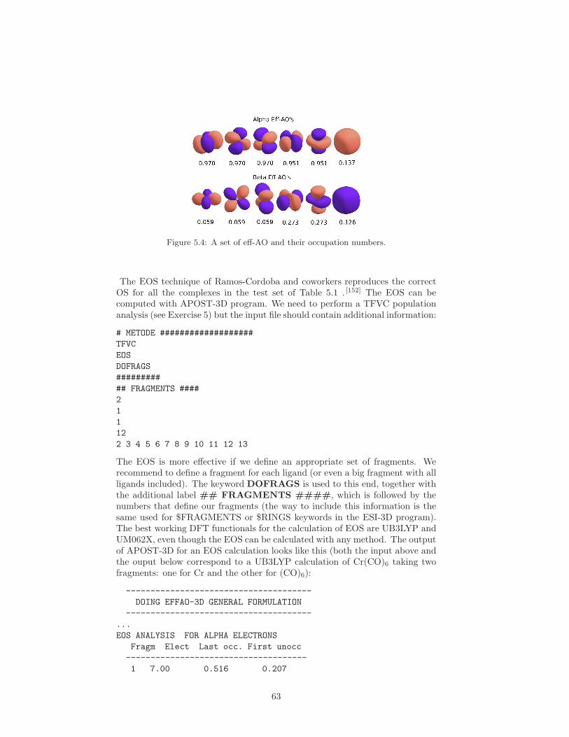
Figure 5.4: A set of eff-AO and their occupation numbers.

The EOS technique of Ramos-Cordoba and coworkers reproduces the correctOS for all the complexes in the test set of Table 5.1 . [152] The EOS can becomputed with APOST-3D program. We need to perform a TFVC populationanalysis (see Exercise 5) but the input file should contain additional information:

# METODE ###################

TFVC

EOS

DOFRAGS

#########

## FRAGMENTS ####

2

1

1

12

2 3 4 5 6 7 8 9 10 11 12 13

The EOS is more effective if we define an appropriate set of fragments. Werecommend to define a fragment for each ligand (or even a big fragment with allligands included). The keyword DOFRAGS is used to this end, together withthe additional label ## FRAGMENTS ####, which is followed by thenumbers that define our fragments (the way to include this information is thesame used for $FRAGMENTS or $RINGS keywords in the ESI-3D program).The best working DFT functionals for the calculation of EOS are UB3LYP andUM062X, even though the EOS can be calculated with any method. The outputof APOST-3D for an EOS calculation looks like this (both the input above andthe ouput below correspond to a UB3LYP calculation of Cr(CO)6 taking twofragments: one for Cr and the other for (CO)6):

--------------------------------------

DOING EFFAO-3D GENERAL FORMULATION

--------------------------------------

...

EOS ANALYSIS FOR ALPHA ELECTRONS

Fragm Elect Last occ. First unocc

-------------------------------------

1 7.00 0.516 0.207

63

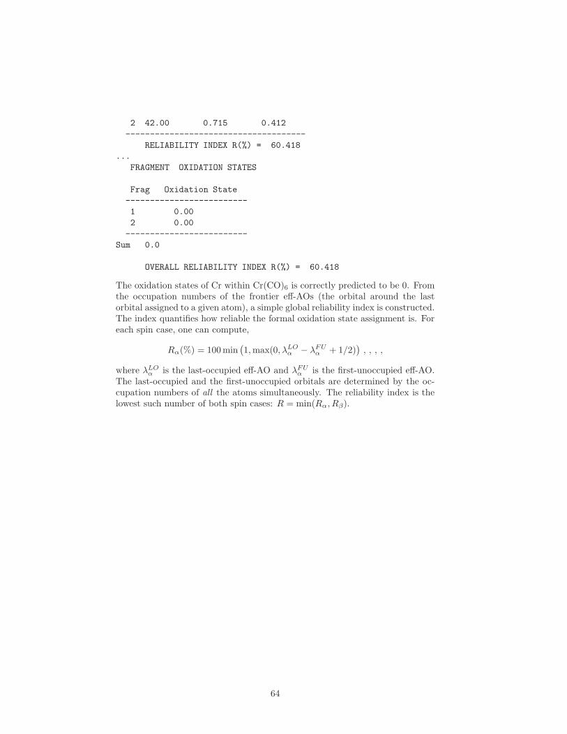
2 42.00 0.715 0.412

-------------------------------------

RELIABILITY INDEX R(%) = 60.418

...

FRAGMENT OXIDATION STATES

Frag Oxidation State

-------------------------

1 0.00

2 0.00

-------------------------

Sum 0.0

OVERALL RELIABILITY INDEX R(%) = 60.418

The oxidation states of Cr within Cr(CO)6 is correctly predicted to be 0. Fromthe occupation numbers of the frontier eff-AOs (the orbital around the lastorbital assigned to a given atom), a simple global reliability index is constructed.The index quantifies how reliable the formal oxidation state assignment is. Foreach spin case, one can compute,

Rα(%) = 100 min(

1,max(0, λLOα − λFU

α + 1/2))

, , , ,

where λLOα is the last-occupied eff-AO and λFU

α is the first-unoccupied eff-AO.The last-occupied and the first-unoccupied orbitals are determined by the oc-cupation numbers of all the atoms simultaneously. The reliability index is thelowest such number of both spin cases: R = min(Rα, Rβ).

64

Chapter 6

The Electron LocalizationFunction (ELF)

The first to recognize the importance of the electron pair in chemical bondingwas Lewis 100 years ago. [65] His model of chemical bonds formed by (shared)electron pairs is one of the most sucessful in modern chemistry. [17] The electronpair is a powerful concept to rationalize and understand the molecular structure,e.g. , through the valence shell electron pair repulsion (VSEPR) theory [154], Theelectron pair concept is found in quantum mechanis through the pair densityor some of its variants. Perhaps a most useful quantity related to the pairdensity is the conditional pair density [155,156]. The definition of the conditionalprobability (CP), i.e. , the probability density of finding electron 2 nearby, 2,when electron 1 is at 1, reads

P (1,2) =ρ2(1,2)

ρ(1)(6.1)

Both the pair density and the CP contain all the necessary information aboutthe relative motion of pairs of electrons. However, the advantage of the CPfunction is that it is actually measuring the probability with respect to theposition of a reference electron and, therefore, is a it is not including the in-formation concerning the position of the reference electron, which is superfluous.

The CP was used by Becke and Edgecombe to define the electron localiza-tion function (ELF) [157]. Namely, they used the spherical average of the CPexpanded by Taylor series around the position of the reference electron

⟨

es·∇P σσ(1,1 + s)⟩

=1

4π

(∫ 1

−1

∫ 2π

0

es∇θdθdφ

)

P σσ(1,1 + s)|s=0

=sin (s∇)

s∇P σσ(1,1 + s)|

s=0(6.2)

which after applying the Taylor expansion of sinh around the reference electro

65

(i.e. , s = 0) gives:

⟨

es·∇P σσ(1,1 + s)⟩

=

(

1 +1

6s2∇2 + . . .

)

P σσ(1,1 + s)|s=0

(6.3)

≈1

6∇2

s Pσσ(1,1 + s)|

s=0(6.4)

Notice that the first term of expansion are zero because of the Pauli principle(ρ2(1,1) = 0) and thus the leading term of the expansion depends on theLaplacian of the CP (or, equivalently, the Laplacian of the pair density). Beckeand Edgecombe used this term as the principal ingredient to construct theELF; namely, they did the ratio between this quantity (Dσ) and the same valuecalculated for the homogenous electron gas (HEG), D0

σ,

D(1) =Dσ(1)

D0σ(1)

=

⟨

es·∇P σσ(1,1 + s)⟩

/((

s2/3)

3/5(6π2)2/3ρ5/6σ

∣

∣

∣

∣

∣

s=0

=∇2

sρ2(1,1 + s)∣

∣

s=0

cF 2ρ8/3σ

(6.5)

where cF = (3/10)(3π2)3/2 is the Fermi constant. The conditional probabilityof finding an electron with spin σ when there is already another electron withthe same spin nearby is lower when the former is localized. Therefore, the ratioin Eq. 6.5 accounts for electron localization, i.e. , the higher it is, the lower thelocalization. Becke an Edgecombe decided to apply a Lorentz transformation tothe previous formulation so that the ELF would be defined in the interval [0, 1].

ELF(1) =1

1 +D(1)2(6.6)

thus ELF=1 corresponds to a completeley localized situation whereas ELF=0is a fully delocalized system and ELF=0.5 is the value that matches the resultfor the HEG. Becke and Edgecombe did their derivation for single-determinantwavefunctions and using the HEG as a reference, however, several authors havegiven a most general (and equivalent!) derivation valid of the ELF for cor-related wavefunctions [158–160] that does not need to use the HEG as a refer-ence. [158,159] The ELF becomes computationally expensive for correlated wave-functions (wavefunction beyond the single-determinant approximation) becauseone should compute the pair density. Opportuntely, there exist some approxi-mations to the pair density that can be used to simplify the calculation of theELF for correlation wavefunction. [161]

6.1 The topological analysis of the electron den-sity

The ELF is a one-coordinate function and likewise the density it admits a topo-logical analysis. The procedure to perform an analysis of the topology of theELF follows the same procedure already described in section 6.1 of this text.The position of the atomic nuclei also correspond to maxima of this function,which often exhibits maxima in other positions. Typically, the ELF is also max-imum in the bonding regions of covalent bonds and in the nonbonded regionswhere electron accumulate, such as the lone pairs. In this regard, ELF basins

66

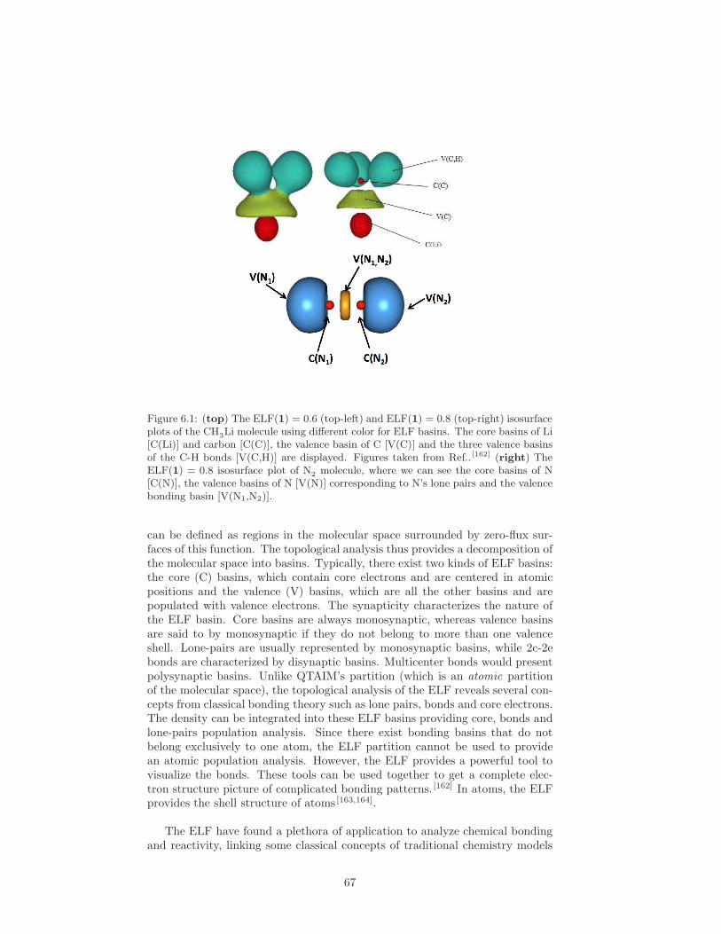
Figure 6.1: (top) The ELF(1) = 0.6 (top-left) and ELF(1) = 0.8 (top-right) isosurfaceplots of the CH3Li molecule using different color for ELF basins. The core basins of Li[C(Li)] and carbon [C(C)], the valence basin of C [V(C)] and the three valence basinsof the C-H bonds [V(C,H)] are displayed. Figures taken from Ref.. [162] (right) TheELF(1) = 0.8 isosurface plot of N2 molecule, where we can see the core basins of N[C(N)], the valence basins of N [V(N)] corresponding to N’s lone pairs and the valencebonding basin [V(N1,N2)].

can be defined as regions in the molecular space surrounded by zero-flux sur-faces of this function. The topological analysis thus provides a decomposition ofthe molecular space into basins. Typically, there exist two kinds of ELF basins:the core (C) basins, which contain core electrons and are centered in atomicpositions and the valence (V) basins, which are all the other basins and arepopulated with valence electrons. The synapticity characterizes the nature ofthe ELF basin. Core basins are always monosynaptic, whereas valence basinsare said to by monosynaptic if they do not belong to more than one valenceshell. Lone-pairs are usually represented by monosynaptic basins, while 2c-2ebonds are characterized by disynaptic basins. Multicenter bonds would presentpolysynaptic basins. Unlike QTAIM’s partition (which is an atomic partitionof the molecular space), the topological analysis of the ELF reveals several con-cepts from classical bonding theory such as lone pairs, bonds and core electrons.The density can be integrated into these ELF basins providing core, bonds andlone-pairs population analysis. Since there exist bonding basins that do notbelong exclusively to one atom, the ELF partition cannot be used to providean atomic population analysis. However, the ELF provides a powerful tool tovisualize the bonds. These tools can be used together to get a complete elec-tron structure picture of complicated bonding patterns. [162] In atoms, the ELFprovides the shell structure of atoms [163,164].

The ELF have found a plethora of application to analyze chemical bondingand reactivity, linking some classical concepts of traditional chemistry models

67

such as the Lewis picture or the resonant structures. [165] The ELF has beenused to analyze all sort of systems, from solids [166] to organometallic com-plexes [167] and its application include aromaticity analysis, [90,168? ] electronicstructure studies along the IRC [169,170] and the mechanism of electrocyclic re-actions, [104,105] among many others. [90,167,171]

The ELF has been implemented in the TopMod package [172] and other codessuch as DGRID. [173] Both program use wavefunction files as those provided byGaussian and Gamess.

68

Chapter 7

The local Spin

Lately, [8,174–178] there has been an interest in assigning local spin values bydecomposing the expectation value of the total spin angular momentum as

〈S 2〉 =∑

A

〈S 2〉A +∑

A,B 6=A

〈S 2〉AB

where A and B are atoms or molecular fragments and 〈S 2〉A is the local spinof fragment A. There are infinitely many ways [177] to define the terms enteringthe r.h.s. of the latter expression. In a recent work some of us have suggesteda proper general definition of 〈S 2〉 that avoids the arbitrarity by imposing anumber of physical requirements and for pure singlet states yields: [177,178]

〈S 2〉A =3

4uA + ΛAA + Λ

′

AA (7.1)

and

〈S 2〉AB = ΛAB + Λ′

AB (7.2)

where the following compact forms in terms of the matrix representation (inmolecular or natural orbitals) of the 1-RDM (D), the 2C (Γ) and the fragmentoverlap matrix (SA) are used,

uA =(

2 Tr(DSA) − Tr(DSAD))

(7.3)

ΛAA =1

2

∑

ijkl

Γij;klSAkiS

Alj Λ

′

AA = −1

2

∑

ijkl

Γij;klSAliS

Akj (7.4)

ΛAB =1

2

∑

ijkl

Γij;klSAkiS

Blj Λ

′

AB = −1

2

∑

ijkl

Γij;klSAliS

Bkj (7.5)

69

Chapter 8

Appendices

8.1 Appendix I: How to perform calculations

The calculations of the ”New Tools For Chemical Bonding Analysis” course willbe performed in the beta cluster of the IQCC. You can find all files of examplesgiven in class in the following folder:

/users/eduard/master

Inside this folder there is a file, aliases, containing all the shortcuts to theprograms that we will use. The list of programs is the following:

• ESI-3D: It is the program we will use to perform the calculation of mul-ticenter and aromaticity indices from the integration files (int-files) calcu-lated with AIMall.

• APOST-3D: We will use this program to calculate effective oxidationstates.

• AIMall: We will use this program to perform topological analyses of theelectron density (QTAIM analysis) and obtain delocalization and localiza-tion indices, as well as the series of atomic overlap matrices collected inthe int-files. The visual part of this program (aimstudio) will be used toobtain the pictures of the critical points of the electron density, countourmaps, isosurfaces of the density and the Laplacian of the electron density.

• Gaussian: We will use this program to obtain the wavefunction file (wfn-file) that AIMall employs in its calculations and the formatted check pointfile (fchk-file) that APOST-3D needs. We will can also obtain a Mullikenpopulation analysis with Gaussian using the keyword pop=full.

How and where to run these programs?

• Gaussian will be run using the queue system, employing the programsand methods given in the previous master courses. We just need to makesure that the wfn-file and fchk-file are copied in our directory after Gaus-sian has ben executed (you should include this command in the scriptyou submitted to the queue). Another possibility is that the first lineof your script enters the directory from which you submit the job, cdname directory.

70

• AIMall can only run in the first node of the cluster (gatchan1 ) becausethe IQCC only owns a one-node license of this program. You can eitherenter this node interactively using the queue command qlogin -clear oryou should submit your jobs to this particular node. This can be doneadding the following termination to the queue name: −−host gatchan1.

• The visual part of AIMall (of which we will only consider aimstudio) hasto run from the visual node. To enter the visual node we should makesure we have entered the cluster using the -X flag, which redirects thegraphical interface and, once we are at the portal of beta, we should type

ssh -X visual

after entering the password of beta we are inside the visual node and weonly need to source the aliases file:

source /users/eduard/aliases

Then we just need to type aimstudio to lunch this program.

• APOST-3D and ESI-3D are in-house programs and can run from anynode in the cluster. The shortcuts to these programs are also available inthe alises file.

8.2 Appendix II: Manual of ESI-3D

ESI-3D program performs the calculation of real-space indices from the AOMsand density matrices (for correlated cases). The AOMs should be collected inseparated files and formatted in the AIMPAC way. Currently ESI-3D acceptsAOMs from AIMPAC, APOST-3D and AIMall. It can perform populationanalysis, calculation of the electron sharing indices, multicenter indices andvarious electronic aromaticity indices (MCI, Iring , FLU, PDI and TREPE).It can decompose these quantities into orbital contributions and permits theconstruction of fragments (groups of atoms).

8.2.1 How to cite the program

Please if you are publishing the results obtained with ESI-3D remember to citecorrectly the program:

Matito, E. ESI-3D: Electron Sharing Indices Program for 3D MolecularSpace Partitioning; Institute of Computational chemistry and Catalysis (IQCC),University of Girona, Catalonia, Spain, 2006; http://iqc.udg.es/ eduard/ESI

and please also cite the papers that deal with the most important featuresof the program:

Matito E., Duran M., Sola M. The aromatic fluctuation index (FLU): A newaromaticity index based on electron delocalization. J. Chem. Phys. 122, 014109

71

(2005)

Matito E., Sola M., Salvador P., Duran M.; Electron Sharing Indexes at theCorrelated Level. Application to Aromaticity Measures. Faraday Discuss. 135,325-345 (2007)

8.2.2 Compulsory keywords

These keywords are only compulsory if $READLOG or $READWFN key-word are not used. If we use $READLOG keyword is because we want toperform a Hilbert space partition analysis and all the information can be ex-tracted from the log file of Gaussian. Therefore, we only need to include thefollowing lines:

$READLOG

name_of_logfile

If we want a real-space analysis and we have the wfn-file or the wfx-filewe can use the keyword $READWFN and the program will retrieve all theimportant information from this file.

$READWFN

name_of_wfnfile

otherwise, we should always include the following keywords:$ATOMS. The number of atoms and the files containing the atomic overlapmatrices.

$ATOMS

number of atoms (n)

file_1.int

file_2.int

...

file_n.int

The user can calculate all the atoms in the molecule are just a small subset ofthem. In the latter case the accuracy of the integration can only be assessedby the value of the Laplacian in the QTAIM partition. In the former case theintegration to the number of electrons, the inspection of the total overlap matrixor the sum rule fulfilled by the delocalization indices can be used as additionacriteria to assess the accuracy of the integration, regardless of the atomic par-tition used.

$BASIS. The number of occupied molecular orbitals (or spinorbitals if open-shell).

$BASIS

number of occupied (spin)orbitals

72

$TYPE. Type of wave function: restricted (hf) or unrestricted (uhf) single-determinant wave function (HF or Kohn-Sham DFT), or natural orbitals (no)expected. If uhf then the program reads the number of the first beta spinorbital.If no the program expects the name of the wavefunction file. If the user hasaccess to DMn program he can also use the dmn-files as input. The wavefunctiontype will be specified as dm1, dm2, dm3 or dm4 and the user will provide thename of this and lower densities (e.g. for dm2 one provides the name of dm1-file first and dm2-file second). For higher order the program will only read thehighest order density matrix file.

$TYPE

hf, uhf, no or dmn

(first beta spinorbital) (wavefunction file) (dm1/dmn file)

(the dm2 file) etc.

8.3 Optional keywords

$AV124. Requests AV124 aromaticity index.

$AV1245. Requests AV1245 aromaticity index.

$DEBUG. Debug-mode on. Provide some extra information to help locatingerrors.

$FLUREFS. It gives the two-center electron sharing indices that should beused as a reference. We will enter them as they appear listed in $RING (makesure to include all rings).

$FMO. Frontier Molecular Orbital analysis. It will print extra information re-garding the FMO. It needs at least the overlap elements involving the LUMOorbital (nb! not provided by default in any program). The FMO numbers aretightly related to the concept of softness kernel (see J. Phys. Chem. A, 115,12459 (2011)). The virtual orbitals are obtained in the wfn/wfx file by addingthe keyword Iop(99/18=-1) in the input file.

$FRAGMENTS. Calculates properties of a user-made fragment. Notice thatpopulation are additive properties, but delocalization/localization are not ad-ditive (delocalization between elements in the fragment are, obviously, not re-flected in the delocalization of the fragment).

$FRAGMENTS

number of fragments

number of atoms in the first fragment (nm1)

1 2 ... nm1 (the atom number according to the order requested)

...

number of atoms in the nth-fragment (nmn)

1 2 ... nmn

$FULLOUT. It produces a full output for ESI-3D. By default some details(FLU specifications, thresholds, etc.) are omitted.

73

$FUZZY. If the program founds this keyword it uses the ESI references calcu-lated with Fuzzy-atom partition for the calculation of FLU.

$GEOMETRY. Inputs the geometry of the molecule in free format (atom sym-bol and three Cartesian coordinates in atomic units). Together with $RING itproduces the HOMA aromaticity index.

$GROUPS. Needed for the orbital decomposition of the ESI and the aromaticindices. First we must provide the number of groups, and afterwards the numberassigned to each orbital according to the group they belong. For σ−π separationof 5 occupied orbitals it might read:

$GROUPS

2

1 1 2 1 2

The decomposition applied is only exact in the case where Sij = 0 for any iand j belonging to different groups (In the case of sigma-pi orbitals separationthe decomposition is only exact for planar molecules). In any other cases thedecomposition cannot be attained exactly and the orbital contributions to theESIs are approximated. We assume the terms Sij(A)Sij(B) can be assignedhalf to orbital i and half to orbital j. Since ideally the overlap between i andj should be zero, the larger the overlap the more crude the approximation. Wecan estimate the error committed in the approximation into two ways: a) bythe absolute sum of the 1

2Sij(A)Sij(B) terms, given in the output as Differ-ence and b) by recalculating the population contribution of different orbitals bysumming up the approximated delocalization indices. Since the decompositionof atomic population into orbitals contributions is exact, by comparison withthese populations from approximate delocalization indices we have an estimateof the error committed. This information is given in the output as Error (frompopulation). If we use the keyword $DEBUG the program will also print theapproximate atomic populations under the columns taged n1, n2, etc. Note thatthe population will be only a good estimate in case we integrate all the atoms inthe molecule, otherwise the sum-rule needs not to be fulfilled and thus there isno guarantee we can reproduce the atomic populations from the delocalizationindices.

In addition, one can specify a negative number of groups. By doing so,one requests a full decomposition (i.e. orbital by orbital, rather than by groupof orbitals) into atomic orbitals. The program will take the negative of thisnumber to estimate the number of basis set to decompose (this integer shouldbe larger than the one specified in $BASIS). The program will produce a filedecompose.out which contains the 2c-ESI and their orbital contributions upto the specified orbital number. Please notice that the program will fail if ittries to read the INT file beyond the number of orbitals included there. Makesure the integration program (FUZZY/PROAIM/etc.) includes the integrationover these many orbitals.

$HIRSH. If the program founds this keyword it uses the references of HIRSHFELD-ESI for the calculation of FLU. Nowadays these references are not included the

74

keyword is left for completeness.

$I-HIRSH. If the program founds this keyword it uses the references of iterative-Hirschfeld-ESI for the calculation of FLU. Nowadays these references are notincluded the keyword is left for completeness.

$MCIALG. Developers option (in progress, unpublished). Use MCIALG and2 below if run into trouble when calculating MCI.$MULLIKEN. We should specify this keyword for the program to performthe correct calculation with Mulliken’s partition (e.g. Mulliken’s atomic overlapmatrices are not symmetric).

$MULTICENTER. Iring and MCI values are printed for all the rings listin $RING. If we want to perform the calculation of these indices for anothercombination of atoms we shall use this keyword.

$MULTICENTER

number of measures

number of atoms in the first measure (nm1)

1 2 ... nm1 (the atom number according to the order requested)

...

number of atoms in the nth-measure (nmn)

1 2 ... nmn

$NELECT. It reads the number of electrons in the molecule. Sometimes (e.g.we do not provide the full list of atoms in the molecule) the program cannotguess correctly this number and we need to provide the correct number.

$NOHYDROGENS. It does not include hydrogens in the output.

$NOMCI. Avoids the MCI calculation.

$NOWARN. Prints no warning messages.

$OVERLAP. Provides a file with partial and total overlap matrices.

$RENORM. Renormalizes the overlaps so that the trace of the total overlapcorresponds to the total number of electrons. This option should only be usedwhen all the atoms in the molecule are integrated.

$RING. Needed for the calculation of aromatic properties. Holds the informa-tion of the connectivity of the ring(s). The program will attemp the calculationof FLU, PDI, HOMA, Iring , MCI, ING and INB . The latter two need the num-ber of π electrons in the ring. The program will retrieve the number from thesecond group of orbitals in GROUPS or take 6 as default, unless the keyword$PI is used. The calculation of MCI and INB involves (n − 1)! calculation,where n is the number of members in the ring. Important: the atoms of eachring must be specified according to the connectivity of each ring.

$RING

75

number of rings (nr)

number of members in the first ring (nm1)

1 2 ... nm1 (the atom number according to their connectivity)

...

number of members in the n-th ring (nmn)

1 2 ... nmn

$TFVC. If the program founds this keyword it uses the references of topologicalfuzzy Voronoi Cell. Nowadays these references are not included the keyword isleft for completeness.

$THRESOUT. Provide the threshold of significant values to be printed in theoutput file.

76

77

Bibliography

[1] C. J. Cramer, Essentials of computational chemistry: theories and models,John Wiley & Sons, 2013.

[2] E. Matito, M. Sola, P. Salvador, and M. Duran, Faraday Discuss. 135,325 (2007).

[3] R. G. Parr and W. Yang, Density-Functional Theory of Atoms andMolecules, Oxford University Press, 1989.

[4] R. F. W. Bader, Atoms in Molecules: A Quantum Theory, Oxford Uni-versity Press, Oxford, 1990.

[5] M. Born, Eur. Phys. J. A 38, 803 (1926).

[6] R. McWeeny, Methods of Molecular Quantum Mechanics, Academic Press,London, second edition, 1989.

[7] P.-O. Lowdin, Phys. Rev. 97, 1474 (1955).

[8] I. Mayer and E. Matito, Phys. Chem. Chem. Phys. 10, 11308 (2010).

[9] K. Ruedenberg, Rev. Mod. Phys. 34, 326 (1962).

[10] X. Fradera, M. A. Austen, and R. F. W. Bader, J. Phys. Chem. A 103,304 (1999).

[11] R. F. W. Bader and M. E. Stephens, Chem. Phys. Lett. 26, 445 (1974).

[12] R. F. W. Bader and M. E. Stephens, J. Am. Chem. Soc. 97, 7391 (1975).

[13] E. Wigner and F. Seitz, Phys. Rev. 46, 509 (1934).

[14] P.-O. Lowdin, Adv. Chem. Phys. 2, 207 (1959).

[15] W. Kutzelnigg and D. Mukherjee, J. Chem. Phys. 110, 2800 (1999).

[16] B. Pullman and A. R. Reisinger, The atom in the history of humanthought, Oxford University Press, USA, 2001.

[17] I. Langmuir, J. Am. Chem. Soc. 41, 868 (1919).

[18] L. Pauling, Proc. Natl. Acad. Sci. U.S.A 14, 359 (1928).

[19] R. S. Mulliken, J. Chem. Phys. 23, 1833 (1955).

78

[20] M. Rodrıguez-Mayorga, E. Ramos-Cordoba, P. Salvador, M. Sola, andE. Matito, Mol. Phys. 114, 1345 (2016).

[21] W. Heyndrickx, P. Salvador, P. Bultinck, M. Sola, and E. Matito, J.Comput. Chem. 32, 386 (2011).

[22] G. Voronoı, Journal fur die reine und angewandte Mathematik 134, 198(1908).

[23] F. L. Hirshfeld, Theor. Chim. Acta (Berlin) 44, 129 (1977).

[24] A. D. Becke, J. Chem. Phys. 88, 2547 (1988).

[25] P. Salvador and E. Ramos-Cordoba, J. Chem. Phys. 139, 071103 (2013).

[26] E. Francisco, A. Martın Pendas, and M. A. Blanco, J. Chem. TheoryComput. 2, 90 (2006).

[27] R. F. W. Bader and P. M. Beddall, J. Chem. Phys. 56, 3320 (1972).

[28] A. M. Pendas, M. A. Blanco, A. Costales, P. M. Sanchez, and V. Luana,Phys. Rev. Lett. 83, 1930 (1999).

[29] J. Poater, M. Sola, and F. M. Bickelhaupt, Chem. Eur. J. 12, 2889 (2006).

[30] R. F. W. Bader, Chem. Eur. J. 12, 2896 (2006).

[31] J. Poater, M. Sola, and F. M. Bickelhaupt, Chem. Eur. J. 12, 2902 (2006).

[32] A. M. Pendas, E. Francisco, M. A. Blanco, and C. Gatti, Chem. Eur. J.13, 9362 (2007).

[33] R. F. W. Bader, J. Phys. Chem. A 102, 7314 (1998).

[34] J. Cioslowski and S. T. Mixon, J. Am. Chem. Soc. 114, 4382 (1992).

[35] J. Cioslowski and S. T. Mixon, Can. J. Chem. 70, 443 (1992).

[36] R. F. W. Bader, J. Phys. Chem. A 113, 10391 (2009).

[37] F. Biegler-Konig and J. Schonbohm, J. Comput. Chem. 23, 1489 (2002).

[38] T. A. Keith, Aimall (version 14.11.23), 2014, TK Gristmill Software,Overland Park KS, USA (aim.tkgristmill.com).

[39] J. Cheeseman, T. A. Keith, and R. F. W. Bader, McMaster University,Hamilton, Ontario 18 (1992).

[40] M. J. Frisch, G. W. Trucks, H. B. Schlegel, G. E. Scuseria, M. A. Robb,J. R. Cheeseman, G. Scalmani, V. Barone, B. Mennucci, G. A. Peters-son, H. Nakatsuji, M. Caricato, X. Li, H. P. Hratchian, A. F. Izmaylov,J. Bloino, G. Zheng, J. L. Sonnenberg, M. Hada, M. Ehara, K. Toyota,R. Fukuda, J. Hasegawa, M. Ishida, T. Nakajima, Y. Honda, O. Kitao,H. Nakai, T. Vreven, J. A. Montgomery, Jr., J. E. Peralta, F. Ogliaro,M. Bearpark, J. J. Heyd, E. Brothers, K. N. Kudin, V. N. Staroverov,R. Kobayashi, J. Normand, K. Raghavachari, A. Rendell, J. C. Burant,S. S. Iyengar, J. Tomasi, M. Cossi, N. Rega, J. M. Millam, M. Klene, J. E.

79

Knox, J. B. Cross, V. Bakken, C. Adamo, J. Jaramillo, R. Gomperts,R. E. Stratmann, O. Yazyev, A. J. Austin, R. Cammi, C. Pomelli, J. W.Ochterski, R. L. Martin, K. Morokuma, V. G. Zakrzewski, G. A. Voth,P. Salvador, J. J. Dannenberg, S. Dapprich, A. D. Daniels, O. Farkas,J. B. Foresman, J. V. Ortiz, J. Cioslowski, and D. J. Fox, Gaussian 09Revision D.01, Gaussian Inc. Wallingford CT 2009.

[41] M. W. Schmidt, K. K. Baldbridge, J. A. Boatz, S. T. Elbert, M. S. Gordon,J. J. Jensen, S. Koseki, N. Matsunaga, K. A. Nguyen, S. Su, T. L. Windus,M. Dupuis, and J. A. Montgomery, J. Comput. Chem. 14, 1347 (1993).

[42] W. Zou, Molden2aim, https://github.com/zorkzou/Molden2AIM.

[43] S. Portmann and H. P. Luthi, CHIMIA 54, 766 (2000).

[44] W. Humphrey, A. Dalke, and K. Schulten, J. Mol. Graphics 14, 33 (1996).

[45] G. Schaftenaar and J. H. Noordik, J. Comput. Aided Mol. Des. 14, 123(2000).

[46] C. Fonseca Guerra, J.-W. Handgraaf, E. J. Baerends, and F. M. Bickel-haupt, J. Comput. Chem. 25, 189 (2004).

[47] P. Bultinck, C. Van Alsenoy, P. W. Ayers, and R. Carbo-Dorca, J. Chem.Phys. 126, 144111 (2007).

[48] P. Bultinck, D. L. Cooper, and D. Van Neck, Phys. Chem. Chem. Phys.11, 3424 (2009).

[49] I. Mayer and P. Salvador, Chem. Phys. Lett. 383, 368 (2004).

[50] P. Salvador and E. Ramos-Cordoba, Apost-3d program, 2012, Universitatde Girona (Spain).

[51] R. F. W. Bader, Chem. Rev. 91, 893 (1991).

[52] R. F. W. Bader, Acc. Chem. Res. 8, 34 (1975).

[53] J. A. Bort and J. B. Rusca, Theoretical and Computational Chemistry:Foundations, methods and techniques, Number 11, Universitat Jaume I,2007.

[54] P. W. Atkins and J. De Paula, (2010).

[55] E. Matito, ESI-3D: Electron sharing indices program for 3D molecu-lar space partitioning, 2015, Institute of Computational Chemistry andCatalysis, University of Girona, Catalonia, Spain.

[56] C. A. Coulson, Proc. R. Soc. London Ser. A 169, 413 (1939).

[57] I. Mayer, Chem. Phys. Lett. 97, 270 (1983).

[58] M. A. Blanco, A. Martın Pendas, and E. Francisco, J. Chem. TheoryComput. 1, 1096 (2005).

[59] I. Mayer and A. Hamza, Theor. Chem. Acc. 105, 360 (2001).

80

[60] P. Salvador, M. Duran, and I. Mayer, J. Chem. Phys. 115, 1153 (2001).

[61] S. F. Vyboishchikov, P. Salvador, and M. Duran, J. Chem. Phys. 122,244110 (2005).

[62] V. Tognetti and L. Joubert, Phys. Chem. Chem. Phys. 16, 14539 (2014).

[63] P. Salvador and I. Mayer, J. Chem. Phys. 120, 5046 (2004).

[64] I. Ruiz, E. Matito, F. J. Holguın-Gallego, E. Francisco, A. M. Pendas,and T. Rocha-Rinza, Theor. Chem. Acc. 135, 209 (2016).

[65] G. N. Lewis, J. Am. Chem. Soc. 38, 762 (1916).

[66] W. N. Lipscomb, Acc. Chem. Res. 6, 257 (1973).

[67] I. Mayer, J. Mol. Struct. (Theochem) 186, 43 (1989).

[68] M. Giambiagi, M. S. de Giambiagi, and K. C. Mundim, Struct. Chem. 1,423 (1990).

[69] A. B. Sannigrahi and T. Kar, Chem. Phys. Lett. 173, 569 (1990).

[70] T. Kar and E. Sanchez Marcos, Chem. Phys. Lett. 192, 14 (1992).

[71] R. Ponec and I. Mayer, J. Phys. Chem. A 101, 1738 (1997).

[72] F. Feixas, M. Sola, J. M. Barroso, J. M. Ugalde, and E. Matito, J. Chem.Theory Comput. 10, 3055 (2014).

[73] K. C. Mundim, M. Giambiagi, and M. S. de Giambiagi, J. Phys. Chem.98, 6118 (1994).

[74] A. B. Sannigrahi and T. Kar, Chem. Phys. Lett. 299, 518 (1999).

[75] M. S. de Giambiagi, M. Giambiagi, and M. S. Fortes, J. Mol. Struct.(Theochem) 391, 141 (1997).

[76] M. Giambiagi, M. S. de Giambiagi, C. D. dos Santos Silva, and A. P.de Figuereido, Phys. Chem. Chem. Phys. 2, 3381 (2000).

[77] P. Bultinck, R. Ponec, and S. Van Damme, J. Phys. Org. Chem. 18, 706(2005).

[78] J. Cioslowski, E. Matito, and M. Sola, J. Phys. Chem. A 111, 6521 (2007).

[79] F. Feixas, E. Matito, J. Poater, and M. Sola, J. Phys. Chem. A 115, 13104(2011).

[80] F. Feixas, E. Matito, J. Poater, F. Maseras, and M. Sola, (in prepara-tion).

[81] P. Bultinck, Faraday Discuss. 135, 347 (2007).

[82] F. Feixas, E. Matito, M. Duran, J. Poater, and M. Sola, Theor. Chem.Acc. 128, 419 (2011).

81

[83] F. Feixas, J. Jimenez-Halla, E. Matito, J. Poater, and M. Sola, J. Chem.Theory Comput. 6, 1118 (2010).

[84] J. O. C. Jimenez-Halla, E. Matito, L. Blancafort, J. Robles, and M. Sola,J. Comput. Chem. 30, 2764 (2009).

[85] F. Feixas, E. Matito, J. Poater, and M. Sola, WIREs, Comput. Mol. Sci.3, 105 (2013).

[86] E. Francisco, A. Martın Pendas, and M. A. Blanco, J. Chem. Phys. 126,094102 (2007).

[87] G. Frenking and A. Krapp, J. Comput. Chem. 28, 15 (2007).

[88] R. Hoffmann, American Scientist 103, 18 (2015).

[89] P. von Rague Schleyer and H. Jiao, Pure Appl. Chem. 68, 209 (1996).

[90] J. Poater, M. Duran, M. Sola, and B. Silvi, Chem. Rev. 105, 3911 (2005).

[91] Z. Chen, C. S. Wannere, C. Corminboeuf, R. Puchta, and P. v. R. Schleyer,Chem. Rev. 105, 3842 (2005).

[92] T. M. Krygowski, H. Szatylowicz, O. A. Stasyuk, J. Dominikowska, andM. Palusiak, Chem. Rev. 114, 6383 (2014).

[93] F. Feixas, E. Matito, J. Poater, and M. Sola, Chem. Soc. Rev. 44, 6389(2015).

[94] A. R. Katritzky, P. Barczynski, G. Musumarra, D. Pisano, and M. Szafran,J. Am. Chem. Soc. 111, 7 (1989).

[95] X. Li, A. E. Kuznetsov, H.-F. Zhang, A. I. Boldyrev, and L.-S. Wang,Science 291, 859 (2001).

[96] A. I. Boldyrev and L.-S. Wang, Chem. Rev. 105, 3716 (2005).

[97] R. Islas, T. Heine, and G. Merino, Acc. Chem. Res. 45, 215 (2011).

[98] A. R. Katritzky, K. Jug, and D. C. Oniciu, Chem. Rev. 101, 1421 (2001).

[99] A. R. Katritzky, M. Karelson, S. Sild, T. M. , and K. Jug, J. Org. Chem.63, 5228 (1998).

[100] T. M. Krygowski and M. K. Cyranski, Chem. Rev. 101, 1385 (2001).

[101] M. K. Cyranski, T. M. Krygowski, A. R. Katritzky, and P. v. R. Schleyer,J. Org. Chem. 67, 1333 (2002).

[102] F. Feixas, E. Matito, J. Poater, and M. Sola, J. Comput. Chem. 29, 1543(2008).

[103] E. Matito, J. Poater, M. Duran, and M. Sola, J. Mol. Struct. (Theochem)727, 165 (2005).

[104] E. Matito, M. Sola, M. Duran, and J. Poater, J. Phys. Chem. B 109, 7591(2005).

82

[105] E. Matito, J. Poater, M. Duran, and M. Sola, Chem. Phys. Chem. 7, 111(2006).

[106] I. Gutman, M. Milun, and N. Trinajstic, J. Am. Chem. Soc. 99, 1692(1977).

[107] M. Garcia-Borras, S. Osuna, M. Swart, J. M. Luis, and M. Sola, Angew.Chem. Int. Ed. 52, 9275 (2013).

[108] X. Lu and Z. Chen, Chem. Rev. 105, 3643 (2005).

[109] A. Osuka and S. Saito, Chem. Commun. 47, 4330 (2011).

[110] F. Feixas, M. Sola, and M. Swart, Can. J. Chem. 87, 1063 (2009).

[111] M.-C. Yoon, P. Kim, H. Yoo, S. Shimizu, T. Koide, S. Tokuji, S. Saito,A. Osuka, and D. Kim, J. Phys. Chem. B 115, 14928 (2011).

[112] E. Marcos, J. M. Anglada, and M. Torrent-Sucarrat, J. Phys. Chem. C116, 24358 (2012).

[113] Z. Liu, Z. Tian, W. Li, S. Meng, L. Wang, and J. Ma, J. Org. Chem. 77,8124 (2012).

[114] M. K. Cyranski, Chem. Rev. 105, 3773 (2005).

[115] H. J. Dauben Jr, J. D. Wilson, and J. L. Laity, J. Am. Chem. Soc. 90,811 (1968).

[116] P. v. R. Schleyer, C. Maerker, A. Dransfeld, H. Jiao, and N. J. v. E.Hommes, J. Am. Chem. Soc. 118, 6317 (1996).

[117] J. Kruszewski and T. M. Krygowski, Tetrahedron Lett. 13, 3839 (1972).

[118] E. Matito, M. Duran, and M. Sola, J. Chem. Phys. 122, 014109 (2005).

[119] J. Poater, X. Fradera, M. Duran, and M. Sola, Chem. Eur. J. 9, 400(2003).

[120] T. M. Krygowski, J. Chem. Inf. Comput. Sci. 33, 70 (1993).

[121] I. Morao, B. Lecea, and F. P. Cossıo, J. Org. Chem. 62, 7033 (1997).

[122] J. O. C. Jimenez-Halla, E. Matito, J. Robles, and M. Sola, J. Organomet.Chem. 691, 4359 (2006).

[123] A. Stanger, J. Org. Chem. 71, 883 (2006).

[124] F. Sondheimer, Pure Appl. Chem. 7, 363 (1963).

[125] C. F. Matta and J. Hernandez-Trujillo, J. Phys. Chem. A 107, 7496(2003).

[126] S. Noorizadeh and E. Shakerzadeh, Phys. Chem. Chem. Phys. 12, 4742(2010).

[127] D. W. Szczepanik, E. Zak, K. Dyduch, and J. Mrozek, Chem. Phys. Lett.593, 154 (2014).

83

[128] D. W. Szczepanik, M. Andrzejak, K. Dyduch, E. Zak, M. Makowski,G. Mazur, and J. Mrozek, Phys. Chem. Chem. Phys. 16, 20514 (2014).

[129] E. Matito, Phys. Chem. Chem. Phys. 18, 11839 (2016).

[130] C. Garcıa-Fernandez, E. Sierda, M. Abadia, B. E. C. Bugenhagen, M. H.Prosenc, R. Wiesendanger, M. Bazarnik, J. E. Ortega, J. Brede, E. Matito,and A. Arnau, J. Phys. Chem. C 121, 27118 (2017).

[131] I. Casademont-Reig, T. Woller, J. Contreras-Garcıa, M. Alonso,M. Torrent-Sucarrat, and E. Matito, Phys. Chem. Chem. Phys. 20, 2787(2018).

[132] E. Matito, M. Duran, and M. Sola, J. Chem. Phys. 125, 059901 (2006).

[133] R. Ponec and F. Uhlik, Croat. Chem. Acta 69, 941 (1996).

[134] C. G. Bollini, M. Giambiagi, M. S. d. Giambiagi, and A. P. de Figuereido,Struct. Chem. 12, 113 (2001).

[135] R. Ponec, P. Bultinck, and A. G. Saliner, J. Phys. Chem. A 109, 6606(2005).

[136] P. Bultinck, M. Rafat, R. Ponec, B. Van Gheluwe, R. Carbo-Dorca, andP. Popelier, J. Phys. Chem. A 110, 7642 (2006).

[137] R. L. Fulton, J. Phys. Chem. 97, 7516 (1993).

[138] R. F. W. Bader, A. Streitwieser, A. Neuhaus, K. E. Laidig, and P. Speers,J. Am. Chem. Soc. 118, 4959 (1996).

[139] E. Matito, J. Poater, M. Sola, M. Duran, and P. Salvador, J. Phys. Chem.A 109, 9904 (2005).

[140] E. Matito, M. Sola, M. Duran, and P. Salvador, J. Phys. Chem. A 110,5108 (2006).

[141] J. M. Mercero, E. Matito, F. Ruiperez, I. Infante, X. Lopez, and J. M.Ugalde, Chem. Eur. J. 21, 9610 (2015).

[142] R. C. Fortenberry, C. M. Novak, J. P. Layfield, E. Matito, and T. J. Lee,J. Chem. Theory Comput. 14, 2155 (2018).

[143] R. Grande-Aztatzi, J. M. Mercero, E. Matito, G. Frenking, and J. M.Ugalde, Phys. Chem. Chem. Phys. 19, 9669 (2017).

[144] R. V. Lopez, O. N. Faza, E. Matito, and C. S. Lopez, Org. Biomol. Chem.15, 435 (2017).

[145] I. A. Popov, F.-X. Pan, X.-R. You, L.-J. Li, E. Matito, C. Liu, H.-J. Zhai,Z.-M. Sun, and A. I. Boldyrev, Angew. Chem. Int. Ed. 128, 15570 (2016).

[146] X. Min, I. A. Popov, F.-X. Pan, L.-J. Li, E. Matito, Z.-M. Sun, L.-S.Wang, and A. I. Boldyrev, Angew. Chem. Int. Ed. 55, 5531 (2016).

[147] J. O. C. Jimenez-Halla, E. Matito, M. Sola, H. Braunschweig, C. Horl,I. Krummenacher, and J. Wahler, Dalton Trans. 44, 6740 (2015).

84

[148] A. C. Castro, E. Osorio, J. L. Cabellos, E. Cerpa, E. Matito, M. Sola,M. Swart, and G. Merino, Chem. Eur. J. 20, 4583 (2014).

[149] P. Karen, P. McArdle, and J. Takats, Pure Appl. Chem. 86, 1017 (2014).

[150] P. Karen, Angew. Chem. Int. Ed. 54, 2 (2014).

[151] A. J. Thom, E. J. Sundstrom, and M. Head-Gordon, Phys. Chem. Chem.Phys. 11, 11297 (2009).

[152] E. Ramos-Cordoba, V. Postils, and P. Salvador, J. Chem. Theory Comput.11, 1501 (2015).

[153] E. Ramos-Cordoba, Development of new tools for local electron distribu-tion analysis, PhD thesis, Univ. Girona, Girona, 2014.

[154] R. J. Gillespie, Coord. Chem. Chem. Rev. 197, 51 (2000).

[155] W. L. Luken and J. C. Culberson, Int. J. Quantum Chem. 16, 265 (1982).

[156] W. L. Luken, J. Chem. Phys. 78, 5729 (1983).

[157] A. D. Becke and K. E. Edgecombe, J. Chem. Phys. 92, 5397 (1990).

[158] M. Kohout, Int. J. Quantum Chem. 97, 651 (2004).

[159] B. Silvi, J. Phys. Chem. A 107, 3081 (2003).

[160] E. Matito, B. Silvi, M. Duran, and M. Sola, J. Chem. Phys. 125, 024301(2006).

[161] F. Feixas, E. Matito, M. Duran, M. Sola, and B. Silvi, J. Chem. TheoryComput. 6, 2736 (2010).

[162] E. Matito, J. Poater, F. M. Bickelhaupt, and M. Sola, J. Phys. Chem. B110, 7189 (2006).

[163] M. Kohout and A. Savin, Int. J. Quantum Chem. 60, 875 (1996).

[164] M. Kohout and A. Savin, J. Comput. Chem. 18, 1431 (1997).

[165] B. Silvi, Phys. Chem. Chem. Phys. 6, 256 (2004).

[166] J. Contreras-Garcıa, A. Martın Pendas, B. Silvi, and J. M. Recio, J. Phys.Chem. Solids 69, 2204 (2008).

[167] E. Matito and M. Sola, Coord. Chem. Rev. 253, 647 (2009).

[168] J. C. Santos, V. Polo, and J. Andres, Chem. Phys. Lett. 406, 393 (2005).

[169] X. Krokidis, S. Noury, and B. Silvi, J. Phys. Chem. A 101, 7277 (1997).

[170] S. Berski, J. Andres, B. Silvi, and L. Domingo, J. Phys. Chem. A 107,6014 (2003).

[171] B. Silvi, I. Fourre, and E. Alikhani, Monatshefte fur Chemie 136, 855(2005).

85

[172] S. Noury, X. Krokidis, F. Fuster, and B. Silvi, Comput. in Chem. 23, 597(1999).

[173] M. Kohout, Dgrid, version 4.6, radebeul, 2011.

[174] A. E. Clark and E. R. Davidson, J. Chem. Phys. 115, 7382 (2001).

[175] I. Mayer, Chem. Phys. Lett. 478, 323 (2009).

[176] D. R. Alcoba, A. Torre, L. Lain, and R. C. Bochicchio, J. Chem. TheoryComput. 7, 3560 (2011).

[177] E. Ramos-Cordoba, E. Matito, I. Mayer, and P. Salvador, J. Chem. The-ory Comput. 8, 1270 (2012).

[178] E. Ramos-Cordoba, E. Matito, P. Salvador, and I. Mayer, Phys. Chem.Chem. Phys. 14, 15291 (2012).

86