NEW THREE AND FOUR NODED PLATE BENDING ELEMENTS

Mikko Lyly and Rolf Stenberg Rakenteiden Mekaniikka, Vol. 27

No. 2, 1994, pp. 3-29

Summary. We report on calculations with two new low-order Reissner-Mindlin plate bending elements obtained by combining a recent stabilization technique with a mixed interpolation of shear strains. The methods are a stabilization of a linear triangular element by Hughes and Taylor and a stabilization of the bilinear quadrilateral method MITC4 by Bathe and Dvorkin.

Introduction Recently considerable progress has been made in the construction of good finite

element methods for "thick" plates with shear deformation. Of the new methods

the "MITC" elements (Mixed Interpolated Tensorial Components), introduced by

Bathe and Dvorkin, have been among the most succesful. They have been reported

to performed excellently in numerous test calculations, cf. [9, 10, 11]. It has also

been possible to give a mathematical error analysis of these methods, cf. [7, 8]

for the analysis in the limiting "Kirchhoff' case and [13] where a complete error

analysis is given. The analysis shows that the methods are stable and of optimal

accuracy if the polynomial order of the methods are at least two.

The bilinear quadrilateral element of this type, the MITC4, is not stable. Nev­

ertheless, it is known to work quite well in practical calculations. In our recent

computational paper [24] we, however, showed that there are cases when the accu­

racy decreases due to the lack of stability.

The linear triangular element that one obtains from the MITC family is an

element that was introduced by Hughes and Taylor [21] (henceforth abbreviated

HT). In their paper it was reported that the element performs well for certain

mesh configurations but badly for others. Hence, the method does not seem to be

reliable enough to be used in practice. From a theoretical standpoint the irregular

behaviour is expected since the method is not stable.

In [13] we, however, showed that both the HT and MITC4 elements can easily

be modified to get elements which are stable and of optimal accuracy. The idea

was to combine the elements with a stabilization technique originally introduced

by Fried and Yang [18] . Recently this technique has been mathematically analyzed

and also generalized in several ways, cf. [26, 20 , 28] .

We should mention that in addition to the elements considered in this paper we

know of only two linear elements for which the convergence have been rigorously

proved; an element by Arnold and Falk [2], and a MITC-type element, mentioned

in [13 , page 145] and independently introduced by Duran and Liberman [15] . In

[17] it was shown that the stabilization technique of Fried and Yang can also be

applied to simplify the Arnold-Falk element. These elements are of the same order

of accuracy as the elements considered here, but for the same mesh they lead to

a greater number of degrees of freedom. Hence, the present elements seem to

be preferable. We should, however, mention that both the original and modified

Arnold-Falk elements work well in practice, cf. [16, 29] where some computational

results are presented.

The purpose of this paper is to present the results of some test calculations

with the stabilized HT and MITC4 elements. We also compare with the results

obtained with the corresponding unstabilized elements and also the "classical"

bilinear element with selectively reduced integration. For the quadrilateral elements

calculations of this type have recently been presented in our paper [24]. Here we

complement this paper by giving the results for other test problems. Computational

results for the triangular element have earlier only been presented in the conference

paper [29]. Here we also present the elements using a notation which might be easier

when considering a computer implementation.

Thick plate theory Let n be the region occupied of the plate and denote by w(.-z;,y) and f3(x,y) =

(f3x (Jy f the transverse deflection and the rotations of the normal of the plate,

respectively. With the given load f the solution to the plate bending problem is

then obtained by minimizing the total potential energy, i.e. it holds [32]

with

II(w,f3) = minii(v,.,.,), (v,>))

(1)

II(v, .,.,) = ~ r (L.,.,lEL.,.,dD + ~ r C\lv- .,.,l G (\lv- .,.,) dD- r .fv dD. (2) 2 lo 2 lo lo

The minimization is performed in the set of all kinematically admissible deflections

and rotations for which the strain energy is finite. For simplicity, we have assumed

4

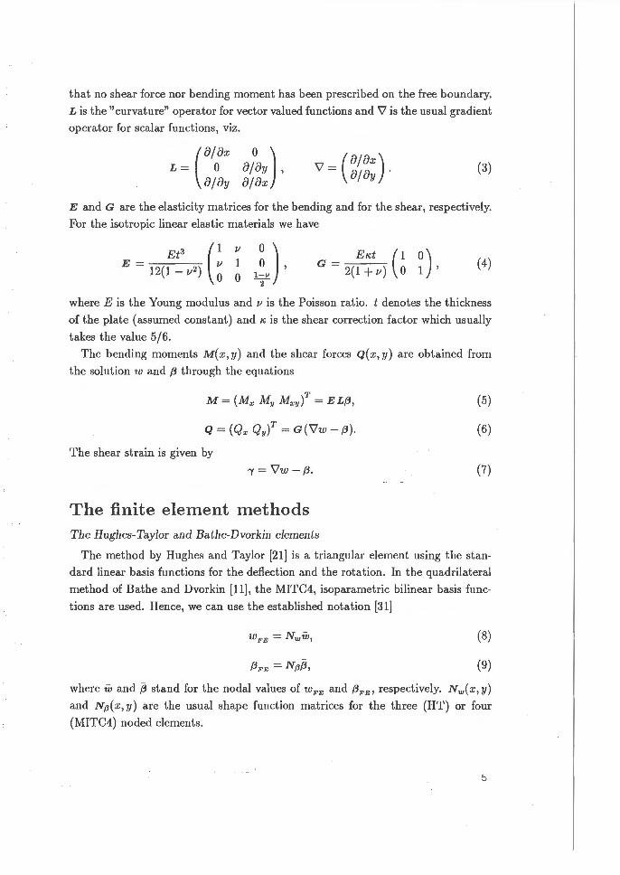
that no shear force nor bending moment has been prescribed on the free boundary.

L is the "curvature" operator for vector valued functions and \1 is the usual gradient

operator for scalar functions, viz.

(a;ax

L= 0 a;ay

'{"7 =(a; ax) v a;ay · (3)

E and G are the elasticity matrices for the bending and for the shear, respectively.

For the isotropic linear elastic materials we have

Et3 ( 1 E = 12(1 - v 2 ) ~

v 1 0

0 ) 0 ' l;v (4)

where E is the Young modulus and v is the Poisson ratio. t denotes the thickness

of the plate (assumed constant) and K is the shear correction factor which usually

takes the value 5/6.

The bending moments M(x,y) and the shear forces Q(x,y) are obtained from

the solution w and {3 through the equations

M = (Mx My Mxyl = E L{3,

Q = (Qx Qyl = G(\lw- /3).

The shear strain is given by

1 = \lw- {3.

The finite element methods The Hughes-Taylor and Bathe-Dvorkin elements

(5)

(6)

(7)

The method by Hughes and Taylor (21] is a triangular element using the stan­

dard linear basis functions for the deflection and the rotation. In the quadrilateral

method of Bathe and Dvorkin [11 J, the MITC4, isoparametric bilinear basis func­

tions are used. Hence, we can use the established notation [31]

(8)

(9)

where wand [3 stand for the nodal values of wFE and {3FE, respectively. Nw(x,y) and NfJ( x, y) are the usual shape function matrices for the three (HT) or four

(MITC4) noded elements.

5

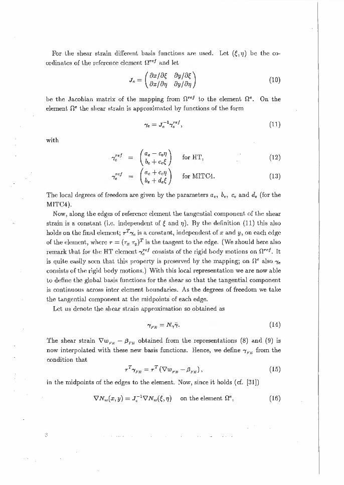
For the shear strain different basis functions are used. Let ( ~, 7]) be the co­

ordinates of the reference element nref and let

_ ( ax 1 a~ oy 1 a~ ) Je- oxlo'l] oyl87]

be the Jacobian matrix of the mapping from nref to the element ne.

element ne the shear strain is approximated by functions of the form

with

ref le

ref le =

for HT,

for MITC4.

(10)

On the

(11)

(12)

(13)

The local degrees of freedom are given by the parameters ae, be, Ce and de (for the

MITC4).

Now, along the edges of reference element the tangential component of the shear

strain is a constant (i.e. independent of~ and 7]). By the definition (11) this also

holds on the final element; rT leis a constant, independent of x and y, on each edge

of the element, where r = ( r., ry)T is the tangent to the edge. (We should here also

remark that for the HT element ,;ef consists of the rigid body motions on nref . It

is quite easily seen that this property is preserved by the mapping; on ne also le

consists of the rigid body motions.) With this local representation we are now able

to define the global basis functions for the shear so that the tangential component

is continuous across inter element boundaries. As the degrees of freedom we take

the tangential component at the midpoints of each edge.

Let us denote the shear strain approximation so obtained as

(14)

The shear strain \lwFE - f3FE obtained from the representations (8) and (9) is

now interpolated with these new basis functions . Hence, we define IFE from the

condition that

(15)

in the midpoints of the edges to the element. Now, since it holds (cf. [31])

(16)

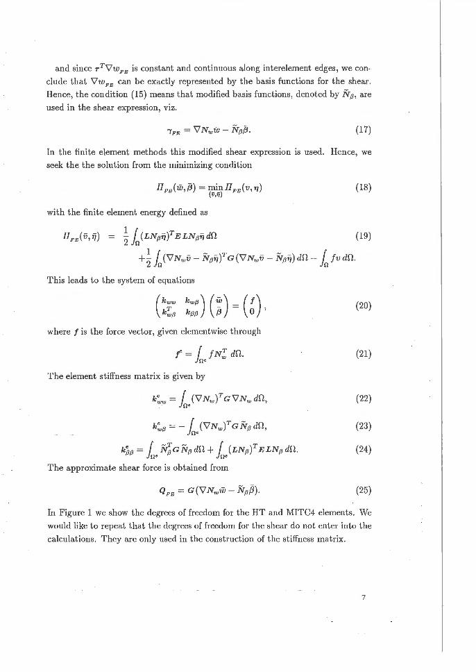
and since -rT"VwFE is constant and continuous along interelement edges, we con­

clude that "VwFE can be exactly represented by the basis functions for the shear.

Hence, the condition (15) means that modified basis functions, denoted by N(J, are

used in the shear expression, viz .

(17)

In the finite element methods this modified shear expression is used. Hence, we

seek the the solution from the minimizing condition

(18)

with the finite element energy defined as

~ { (LN(Jiif E LN(Jij dO (19) 2 Jo

+~ r ("VNwV- N(Jr,f G ('\1 NwV- Npij) dO- r fv dO . 2Jo Jo

This leads to the system of equations

(20)

where f is the force vector, given elementwise through

f = f fN~ dO. Jo•

(21)

The element stiffness matrix is given by

(22)

(23)

(24)

The approximate shear force is obtained from

(25)

In Figure 1 we show the degrees of freedom for the HT and MITC4 elements. We

would like to repeat that the degrees of freedom for the shear do not enter into the

calculations. They are only used in the construction of the stiffness matrix.

7

e deflection

Q rotation vector

- tangential component of the shear strain vector

Figure 1: Degrees of freedom for the HT and MITC4 elements and their stabilized modifications.

The Hughes- Taylor element with reduced integration

In [21] it was shown that the HT element performs better if the energy expression

is calculated inexactly with the midpoint rule. The method obtained is then given

by (20) with

k~w = (Y'Nw(x.,y.)fGV'Nw(x.,y.)A., (26)

k~{) = -(V'Nw(x.,y.)fGN{)(x.,y.) A., (27)

k~{J = N{)(x.,y.)TGN(J(x.,y.)Ae + (LN(J(xe ,Ye)fELN[J(x.,y.)A., (28)

where ( x. , y.) is the midpoint of the element n• and Ae is its area. We remark that

the bending energy is still evaluated exactly by this. The shear force is piecewise

constant given by

The stabilized Hughes- Taylor and Bathe-Dvorkin elements {13, 24}

The stabilized methods are obtained in a very simple way, in the discrete en­

ergy expression (19) the shear elasticity matrix G is replaced with the following

modification

8

GFE=( 2 t2

h2)G ontheelementn•. i + Q e

(30)

Here h. is the length of the diameter of the element ne and a is a positive parameter.

The stiffness matrix obtained is as in (20) with

k~f3 =- f (VNwf GFENf3 dD, Joe

k~{3 = { IqGFENf3df1+ { (LNf3)TELNf3df1 . Joe Joe

(31)

(32)

(33)

With a = 0 we recover the original elements. Note also that when the mesh size

approach zero the modified methods converge towards the original ones.

The shear force is given by (note that GFE varies from element to element)

(34)

The quadrilateral method with selective reduced integra.tion {19}

In the quadrilateral method with selective reduced integration an inexact mid­

point integration rule is used for the shear term. Hence, the stiffness matrix of the

method is as in (20) with

k~f3 = -(\lNw(xe,Ye))T G Nf3(xe, Ye) Ae, (36)

k~{3=Nf3(Xe,YefGNf3(xe,Ye)Ae+ { (LNf3fELNf3df1 , (37) Joe where again (xe, Ye) and Ae are the midpoint and the area of ne, respectively.

The shear force is given by

Error estimates for the tnethods In this section we will review the known theoretical results with respect to the

convergence of the methods. When studying the convergence and locking, one has

to consider a sequence of problems for which the load varies as f = t 3g with the

function g fixed. With this the exact solution to (1) has a nonvanishing and finite

limit when t ---t 0. For a well designed locking-free element the convergence should

be independent of the plate thickness t for this sequence of problems. The error

9

estimates proved for finite element methods are usually given in "L2 -norms", i.e.

the norms defined by (cf. [31, page 401])

{ llvll£2 = [fn V

2 dr2]11\

II11IIL2 = [In 1JT 1J dr2]112

for scalar functions,

for vector valued functions.

The error estimates are given with the mesh parameter (cf. [19, 31])

(39)

( 40)

For the MITC4 it is possible to prove error estimates for a particular class of meshes

for which the region is first divided into quadrilateral subregions and then every

subregion is regularly divided into quadrilaterals (we refer to [27] for the exact

statement of this). For this class of meshes it has been possible to prove that

[7, 8, 13]

( 41)

and

( 42)

For the case when the elements are rectanguar it additionally holds [7, 8]

( 43)

Here C denotes different positive constants which only depend on the exact solution

to the problem. The constants are independent of the plate thickness t which means

that the method will not lock (for this particular class of meshes). We remark that

for a method that locks, the usual error analysis would lead to estimates as above

with C -t oo, when t -t 0. For the above estimates to be valid it is required that

the L2-norm of all second partial derivatives of the deflection and the rotation are

bounded.

In the error analysis the estimates are given for the scaled shear force q = t-3 Q

since it is this quantity that has a finite non-vanishing limit when t -t 0 (with the

above scaling of the load). For this quantity the best estimate obtained is (this

estimate can be derived by combining results from [13, 22, 27] ) (below c will denote

different positive constants)

(44)

We see that for very thin plates the shear obtained with the MITC4 may be highly

unreliable. That this is the case we will show by our numerical examples.

10

For the HT element (with both exact and reduced integration) there has not

been presented any error estimates. In fact, an attempt to perform an analysis

reveals that the element cannot be very good. That this is the case will be shown

in the next section.

For the stabilized MITC4 and HT a complete error analysis can be given, cf. [13].

The methods will converge optimally, the estimates ( 41) and ( 42) hold for general

finite element meshes. For the shear the following estimate is derived, which also

is optimal,

llq- qFE ll£2 ~ c ( t: h) ' ( 45)

We see that the shear does not necessarily have to converge, but it stays bounded

independent of the plate thickness.

For the quadrilateral method with selective reduced integration an error analysis

was presented in [22]. They proved both the estimates (41) and (42) but under

very restrictive conditions; the elements have to be rectangular and much more

smoothness is required of the exact solution. The estimate for the shear they

obtained is

llq- qFEIIL2 ~ C c /ch3 ) · ( 46)

Hence, the shear obtained with that method cannot, in general, be very good.

Numerical results We perform all our numerical tests for one geometrical confi guration, a square

plate of unit side length occupying the region n = [0, 1] x [0, 1]. In all cases the

loading and boundary conditions will be symmetric so that only one quarter of

the plate will be analyzed. The physical parameters are chosen as E = 1 and

v = 0.3. For the shear correction factor we take the usual value1 K = 5/6. The

stability parameter is taken as a= 0.1 for the stabilized MITC4 and a= 0.2 for

the stabilized HT.

Convergence studies for regular and irregular meshes

In the first test case the plate is subject to a uniform load acting on the area

[3/8 ,5 / 8] X [3/8,5 / 8]. As the boundary conditions we choose the "hard" simply

supported case, i.e. both the deflection and the tangential component of the rota­

tion vanish on the boundary. With this choice all the variables of interest converge

1 Below we will show that the stabilized methods are the methods that work best. In those the shear term is modified quite much, and hence the value of the shear correction factor seems to be a rather irrelevant question.

11

I CL

~--,---~--~~~~

CL

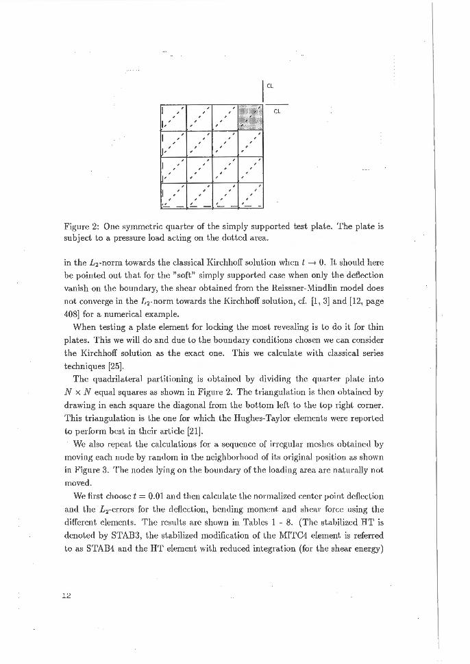
Figure 2: One symmetric quarter of the simply supported test plate. The plate is subject to a pressure load acting on the dotted area.

in the L2-norm towards the classical Kirchhoff solution when t --+ 0. It should here

be pointed out that for the "soft" simply supported case when only the deflection

vanish on the boundary, the shear obtained from the Reissner-Mindlin model does

not converge in the L2-norm towards the Kirchhoff solution, cf. [1, 3] and [12, page

408] for a numerical example.

When testing a plate element for locking the most revealing is to do it for thin

plates. This we will do and due to the boundary conditions chosen we can consider

the Kirchhoff solution as the exact one. This we calculate with classical series

techniques [25].

The quadrilateral partitioning is obtained by dividing the quarter plate into

N x N equal squares as shown in Figure 2. The triangulation is then obtained by

drawing in each square the diagonal from the bottom left to the top right corner.

This triangulation is the one for which the Hughes-Taylor elements were reported

to perform best in their article [21].

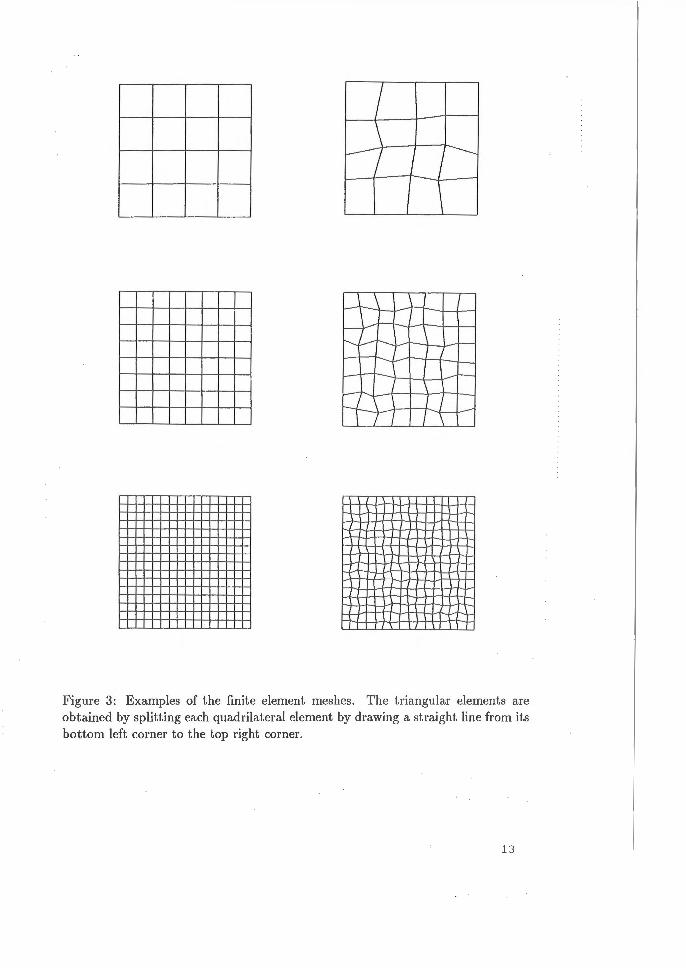
We also repeat the calculations for a sequence of irregular meshes obtained by

moving each node by random in the neighborhood of its original position as shown

in Figure 3. The nodes lying on the boundary of the loading area are naturally not

moved.

We first choose t = 0.01 and then calculate the normalized center point deflection

and the L2-errors for the deflection, bending moment and shear force using the

different elements. The results are shown in Tables 1 - 8. (The stabili zed HT is

denoted by STAB3, the stabilized modification of the MITC4 element is referred

to as STAB4 and the HT element with reduced integration (for the shear energy)

12

1--7 ---1

I

-+ '- ~ -.., --}-~1-4-T-~~~

-+---' 1-

--, I '--

-I

Figure 3: Examples of the finite element meshes . The triangular elements are obtained by splitting each quadrilateral element by drawing a straight line from its bottom left corner to the top right corner.

13

is abbreviated as HTRI).

In Tables 3 and 4, INT denotes the Lagrange interpolant for the deflection (i.e.

a finite element deflection with exact nodal values). In Tables 5 and 6, INT means,

however, the bending moment calculated from the Lagrange interpolant for the

rotation . The normalized LTerrors for the interpolants are shown in order to

approximately define the "best possible level" for the results obtained by using the

finite elements - if the interpolant is bad then there is no reason to expect a good

finite element solution either.

Table 1. The normalized centerpoint deflections wFE ( center)/w( center) for the regular and irregular meshes with t = 0.01 . Three noded elements.

STAB3 HT HTRI N Regular Irregular Regular Irregular Regular Irregular

4 0.9670 8 0.9925 16 0.9988

0.9648 0.9916 0.9986

0.6910 0.9602 0.9946

0.6713 0.9578 0.9942

0.8922 0.8816 0.9801 0.9780 0.9959 0.9956

Table 2. The normalized centerpoint deflections wFE(center)/w(center) for the regular and irregular meshes with t = 0.01. Four noded elements.

STAB4 MITC4 SRI N Regular Irregular Regular Irregular Regular Irregular

4 1.0013 1.0057 0.9758 0.9784 0.9759 0.9452 8 1.0012 1.0012 0.9950 0.9940 0.9950 0.9220 16 1.0009 1.0009 0.9994 0.9991 0.9994 0.9744

Table 3. The L2-errors llw- wFEIIL2 /IIwiiL2 for the regular and irregular meshes with t = 0.01. Three noded elements.

STAB3 HT HTRI INT N Regular Irregular Regular Irregular Regular Irregular Regular Irregular

4 0.0503 0.0524 0.3112 0.3327 0.1106 0.1235 0.0249 0.0260 8 0.0123 0.0135 0.0416 0.0424 0.0211 0.0228 0.0063 0.0070 16 0.0026 0.0029 0.0059 0.0064 0.0046 0.0050 0.0016 0.0017

14

Table 4. The L2-errors Jlw - wFEI IL2 / II wJIL2 for the regular and irregular meshes with t = 0.01. Four noded elements.

STAB4 MITC4 SRI INT N Regular Irregular Regular Irregular Regular Irregular Regular Irregular

4 0.0208 0.0191 0.0372 0.0365 0.0372 0.0719 0.0274 0.0274 8 0.0049 0.0056 0.0090 0.0103 0.0090 0.0863 0.0069 0.0077 16 0.0009 0.0010 0.0018 0.0021 0.0018 0.0262 0.0017 0.0019

As we can see from the tables above, the HT element and its modified version

with reduced integration lock severely in the case of the coarsest mesh with N = 4.

For N = 8 and N = 16 the results are better, but still much less accurate than

those obtained with the stabilized version. For the stabilized method the deflection

is optimally convergent and almost as good as the interpolant in each case.

The four noded SRI element gives a very good deflection with regular meshes

but the accuracy is completely destroyed when the mesh is distorted; the error in

deflection is larger for N = 8 than it is for N = 4, and for N = 16 the £ 2-error for

the irregular mesh is ten times as big as for the regular mesh. That this happens

is clearly a sign of the lack of stability of this method. The original MITC4 does

not lock in this benchmark example, but still the accuracy is not as good as for its

stabilized modification. The stabilized MITC4 gives here the best approximation

(better than the interpolant) for the deflection, even for the irregular and coarse

meshes.

Table 5. The L2-errors liM- MFE IIL2 /IIMJIL2 for the regular and irregular meshes with t = 0.01. Three noded elements.

STAB3 HT HTRI INT N Regular Irregular Regular Irregular Regular Irregular Regular Irregular

4 0.1997 0.2054 0.3511 0.3814 0.2179 0.2290 0.1923 0.1968 8 0.0987 0.1004 0.1057 0.1129 0.0996 0.1029 0.0975 0.0991 16 0.0490 0.0504 0.0493 0.0514 0.0492 0.0506 0.0490 0.0502

15

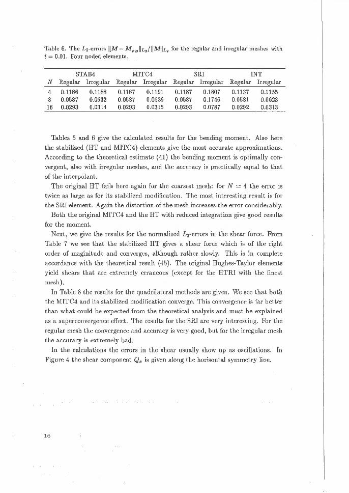
Table 6. The L2-errors liM- MFE II£2 / IIMIIL2 for the regular and irregular meshes with t = 0.01. Four noded elements.

STAB4 MITC4 SRI INT N Regular Irregular Regular Irregular Regular Irregular Regular Irregular

4 0.1186 0.1188 0.1187 0.1191 0.1187 0.1807 0.1137 0.1155 8 0.0587 0.0632 0.0587 0.0636 0.0587 0.1746 0.0581 0.0623 16 0.0293 0.0314 0.0293 0.0315 0.0293 0.0787 0.0292 0.0313

Tables 5 and 6 give the calculated results for the bending moment. Also here

the stabilized (HT and MITC4) elements give the most accurate approximations.

According to the theoretical estimate ( 41) the bending moment is optimally con­

vergent , also with irregular meshes, and the accuracy is practically equal to that

of the interpolant.

The original HT fails here again for the coarsest mesh: for N = 4 the error is

twice as large as for its stabilized modification. The most interesting result is for

the SRI element. Again the distortion of the mesh increases the error considerably.

Both the original MITC4 and the HT with reduced integration give good results

for the moment.

Next, we give the results for the normalized L2-errors in the shear force. From

Table 7 we see that the stabilized HT gives a shear force which is of the r ight

order of maginitude and converges, although rather slowly. This is in complete

accordance with the t heoretical result (45). T he original Hughes-Taylor elements

yield shears that are extremely erraneous (except for the HTRI with the finest

mesh).

In Table 8 the results for the quadrilateral methods are given. We see that both

the MITC4 and its stabilized modification converge. This convergence is far better

than what could be expected from the theoretical analysis and must be explained

as a superconvergence effect . The results for the SRI are very interest ing. For the

regular mesh the convergence and accuracy is very good , but for the irregular mesh

the accuracy is extremely bad.

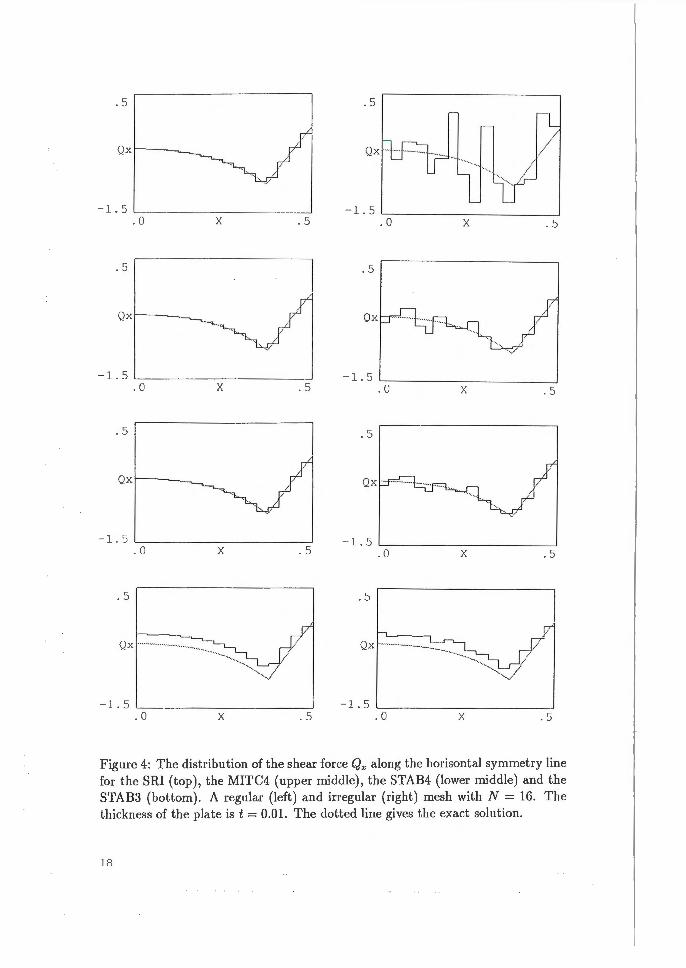
In the calculations the errors in the shear usually show up as oscillations. In

Figure 4 the shear component Qx is given along the horisontal symmetry line.

16

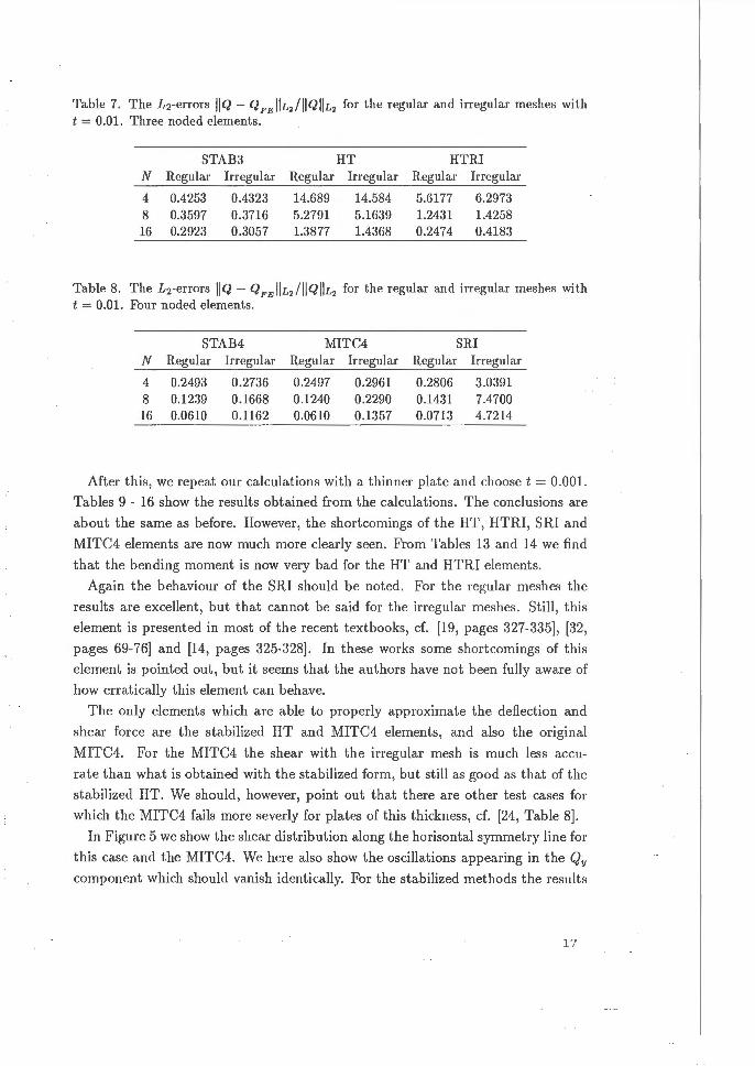
Table 7. The L2-errors IIQ - Q FE 11£,/IIQIIL, for the regular and irregular meshes with t = 0.01. Three noded elements.

STAB3 HT HTRI N Regular Irregular Regular Irregular Regular Irregular

4 0.4253 0.4323 14.689 14.584 5.6177 6.2973 8 0.3597 0.3716 5.2791 5.1639 1.2431 1.4258 16 0.2923 0.3057 1.3877 1.4368 0.2474 0.4183

Table 8. The L2-errors IIQ- QFEIIL,/IIQIIL, for the regular and irregular meshes with t = 0.01. Four noded elements.

STAB4 MITC4 SRI N Regular Irregular Regular Irregular Regular Irregular

4 0.2493 0.2736 0.2497 0.2961 0.2806 3.0391 8 0.1239 0.1668 0.1240 0.2290 0.1431 7.4700 16 0.0610 0.1162 0.0610 0.1357 0.0713 4.7214

After this, we repeat our calculations with a thinner plate and choose t = 0.001.

Tables 9 - 16 show the results obtained from the calculations. The conclusions are

about the same as before. However, the shortcomings of the HT, HTRI, SRI and

MITC4 elements are now much more clearly seen. From Tables 13 and 14 we find

that the bending moment is now very bad for the HT and HTRI elements.

Again the behaviour of the SRI should be noted. For the regular meshes the

results are excellent, but that cannot be said for the irregular meshes. Still, this

element is presented in most of the recent textbooks, cf. [19, pages 327-335], [32,

pages 69-76] and [14, pages 325-328]. In these works some shortcomings of this

element is pointed out, but it seems that the authors have not been fully aware of

how erratically this element can behave.

The only elements which are able to properly approximate the deflection and

shear force are the stabilized HT and MITC4 elements, and also the original

MITC4. For the MITC4 the shear with the irregular mesh is much less accu­

rate than what is obtained with the stabilized form, but still as good as that of the

stabilized HT. We should, however, point out that there are other test cases for

which the MITC4 fails more severly for plates of this thickness, cf. [24, Table 8].

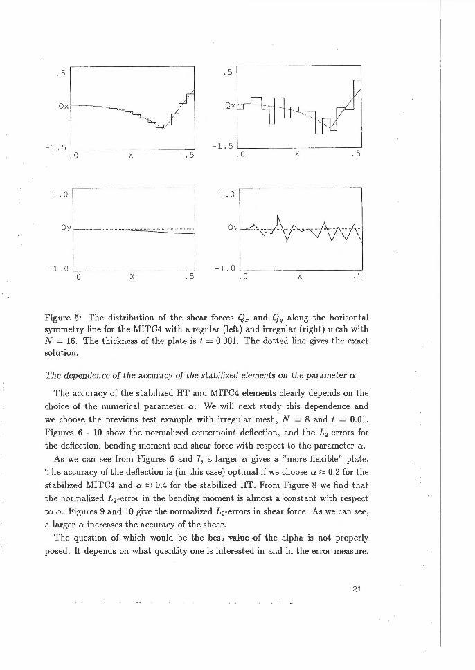
In Figure 5 we show the shear distribution along the horisontal symmetry line for

this case and the MITC4. We here also show the oscillations appearing in the Qy

component which should vanish identically. For the stabilized methods the results

17

.5 . 5

Qxr-----

-1.5 L---------------------~ . 0 X . 5

. 5 . 5

Qxr-----

- 1.5 L_ ____________________ _

.0 X . 5 -1.5 ~--------------------­

.0 X . 5

.5 . 5

Qx r-----

- 1 . 5 L_ ____________________ ~

. 0 X . 5 -1 . 5 L---------------------~ .0 X .5

. 5 . 5

Qx. --·--

-1 . 5 L_ ____________________ _ -1. 5 L_ ________________ . _ __ __j

.0 X .5 . 0 X . 5

Figure 4: The distribution of the shear force Qx along the horisontal symmetry line for the SRI (top) , the MITC4 (upper middle), the STAB4 (lower middle) and the STAB3 (bottom). A regular (left) and irregular (right) mesh with N = 16. The thickness of the plate is t = 0.01. The dotted line gives the exact solution.

18

are as in Figure 4. The shear for the SRI with the irregular mesh is so highly

oscillating that there is not any point in showing it. For the regular mesh the SRI

gives a shear which is very near that of the MITC4.

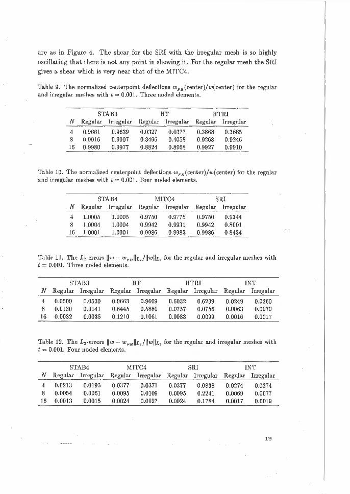
Table 9. The normalized centerpoint deflections wFE( center )/w( center) for the regular and irregular meshes with t = 0.001. Three noded elements.

STAB3 HT HTRI N Regular Irregular Regular Irregular Regular Irregular

4 0.9661 0.9639 0.0327 0.0377 0.3868 0.3685 8 0.9916 0.9907 0.3496 0.4058 0.9268 0.9246 16 0.9980 0.9977 0.8824 0.8968 0.9927 0.9910

Table 10. The normalized centerpoint deflections wFE(center)/w(center) for the regular and irregular meshes with t = 0.001. Four noded elements.

STAB4 MITC4 SRI N Regular Irregular Regular Irregular Regular Irregular

4 1.0005 1.0005 0.9750 0.9775 0.9750 0.9344 8 1.0004 1.0004 0.9942 0.9931 0.9942 0.8001 16 1.0001 1.0001 0.9986 0.9983 0.9986 0.8434

Table 11. The L2-errors llw- wFE IIL2 /II wii L2 for the regular and irregular meshes with t = 0.001. Three noded elements.

STAB3 HT HTRI INT N Regular Irregular Regular Irregular Regular Irregular Regular Irregular

4 0.0509 0.0530 0.9663 0.9609 0.6032 0.6239 0.0249 0.0260 8 0.0130 0.0141 0.6445 0.5880 0.0757 0.0756 0.0063 0.0070 16 0.0032 0.0035 0.1210 0.1061 0.0083 0.0099 0.0016 0.0017

Table 12. The L2-errors llw - wFE IIL2 /llwll£2 for the regular and irregular meshes with t = 0.001. Four noded elements.

STAB4 MITC4 SRI INT N Regular Irregular Regular Irregular Regular Irregular Regular Irregular

4 0.0213 0.0195 0.0377 0.0371 0.0377 0.0838 0.0274 0.0274 8 0.0054 0.0061 0.0095 0.0109 0.0095 0.2241 0.0069 0.0077 16 0.0013 0.0015 0.0024 0.0027 0.0024 0.1784 0.0017 0.0019

19

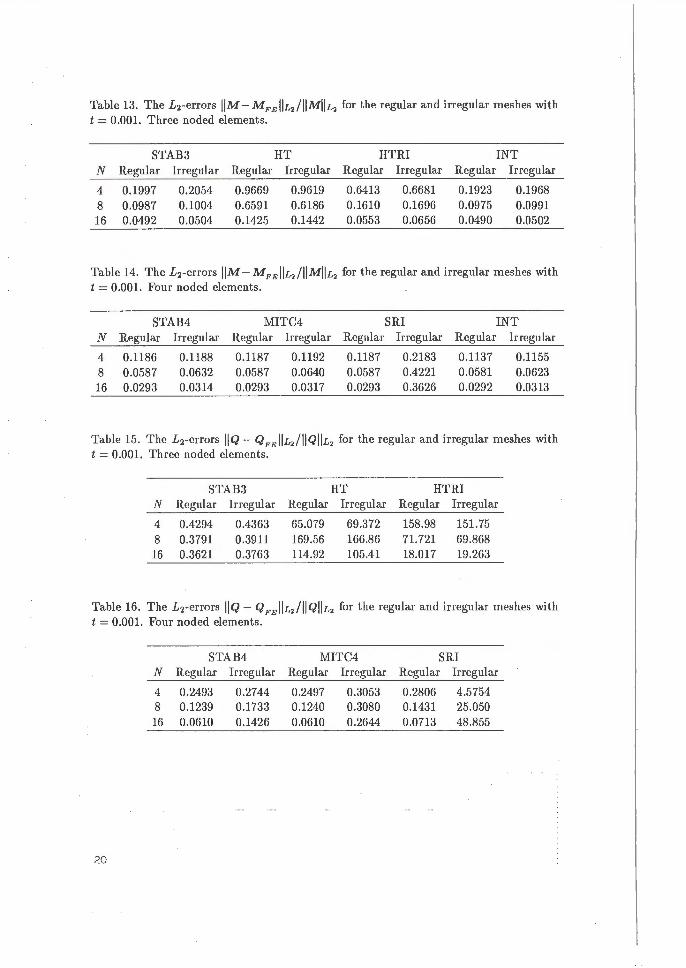
Table 13. The L2-errors liM- M FE IIL2 /IIMIIL2 for the regular and irregular meshes with t = 0.001. Three noded elements.

STAB3 HT HTRI INT N Regular Irregular Regular Irregular Regular Irregular Regular Irregular

4 0.1997 0.2054 0.9669 0.9619 0.6413 0.6681 0.1923 0.1968 8 0.0987 0.1004 0.6591 0.6186 0.1610 0.1696 0.0975 0.0991 16 0.0492 0.0504 0.1425 0.1442 0.0553 0.0656 0.0490 0.0502

Table 14. The L2-errors liM- M FE IIL2 /IIMIIL2 for the regular and irregula.r meshes with t = 0.001. Four noded elements.

STAB4 MITC4 SRI INT N Regular Irregular Regular Irregular Regular Irregular Regular Irregular

4 0.1186 0.1188 0.1187 0.1192 0.1187 0.2183 0.1137 0.1155 8 0.0587 0.0632 0.0587 0.0640 0.0587 0.4221 0.0581 0.0623 16 0.0293 0.0314 0.0293 0.0317 0.0293 0.3626 0.0292 0.0313

Table 15. The L2-errors IIQ- QFEII£2 /IIQII£2 for the regular and irregular meshes with t = 0.001. Three noded elements.

STAB3 HT HTRI N Regular Irregular Regular Irregular Regular Irregular

4 0.4294 0.4363 65.079 69.372 158.98 151.75 8 0.3791 0.3911 169.56 166.86 71.721 69.868 16 0.3621 0.3763 114.92 105.41 18.017 19.263

Table 16. The L2-errors IIQ- QFEIIL2 /IIQIIL2 for the regular and irregular meshes with t = 0.001. Four noded elements.

20

STAB4 MITC4 SRI N Regular Irregular Regular Irregular Regular Irregular

4 0.2493 8 0.1239 16 0.0610

0.2744 0.1733 0.1426

0.2497 0.1240 0.0610

0.3053 0.3080 0.2644

0.2806 0.1431 0.0713

4.5754 25.050 48.855

. 5 .5

Qxr---~

-1. 5 t__ __________ _, -1 . 5 '-------------~ .0 X .5 . 0 . 5

1.0 1 .0

Qy

-1.0 . 0 X .5

- 1 . 0 '-------------~ . 0 X . 5

Figure 5: The distribution of the shear forces Qx and Qy along the horisontal symmetry line for the MITC4 with a regular (left) and irregular (right) mesh with N = 16. The thickness of the plate is t = 0.001. The dotted line gives the exact solution.

The dependence of the accuracy of the stabilized elements on the parameter a

The accuracy of the stabilized HT and MITC4 elements clearly depends on the

choice of the numerical parameter a. We will next study this dependence and

we choose the previous test example with irregular mesh, N = 8 and t = 0.01.

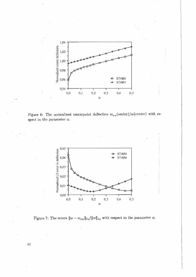
Figures 6 - 10 show the normalized centerpoint deflection, and the L2-errors for

the deflection, bending moment and shear force with respect to the parameter a.

As we can see from Figures 6 and 7, a larger a gives a "more flexible" plate.

The accuracy of the deflection is (in this case) optimal if we choose a~ 0.2 for the

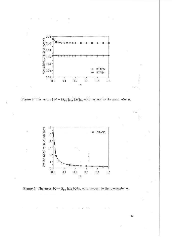
stabilized MITC4 and a~ 0.4 for the stabilized HT. From Figure 8 we find that

the normalized Lrerror in the bending moment is almost a constant with respect

to a. Figures 9 and 10 give the normalized L2-errors in shear force. As we can see,

a larger a increases the accuracy of the shear.

The question of which would be the best value of the alpha is not properly

posed. It depends on what quantity one is interested in and in the error measure.

21

1,04 -r--------------~

c: g

E 1.02 c "' '0

g 1,00 ;} 0

"8 0 98 .~ '

"' E ~ 0,96

-+- STAB4

0,94 +---r-------.----,----r-----1

0,0 0,1 0 ,2 0,3 0,4 0,5

a.

Figure 6: The normalized centerpoint deflection wFE(center)/w(center) with re­spect to the parameter a.

c: 0,05 .9 0 -e- STAB3 "' '5 0,04 -+- STAB4 '0

= :som t:: 0

,-:, :;o,Q2 "' N

~ EO,Ql .... 0 z

0,00 0,0 0,1 0,2 0,3 0,4 0,5

a

Figure 7: The errors llw- wFEII£2 /IIwll£2 with respect to the parameter a.

22

0,12 ..... ----------------.,

~00·~ ...... o ,I E

·5 008 ~ '

c-!l 0,06 ....l

"2 .!::> 0,04 til

§ 0,02 z

-e- STAB3 ...... STAB4

0,00 -+----.----..------,.----,-----t 0,0 0 ,1 0 ,2 0,3 0,4 0.5

(1.

Figure 8: The errors liM- MFE IIL2 /IIMIIL2 with respect to t he parameter a .

<!) 6 0 .... .8 -1:1- STAB3 ~ 5 <!) ..c "' .5 4 .... 0 t::

3 <!)

c-!l ....l "0 2 <!) N

~ E 0 z

0

0,0 0,1 0,2 0,3 0,4 0,5

(1.

Figure 9: The error IIQ- QFEIIL2 /IIQIIL2 with respect to the parameter a.

23

~ 0,24

..8 ~ 0,22

..c: Vl

.5 (; 0,20 t: ..,

01 ....l 0,18 ""8 N

~ 0,16 .... 0 z

-a- STAB4

0,14 +---.,.----..-----,r---------r---1

0,0 0,1 0,2 0,3 0,4 0,5

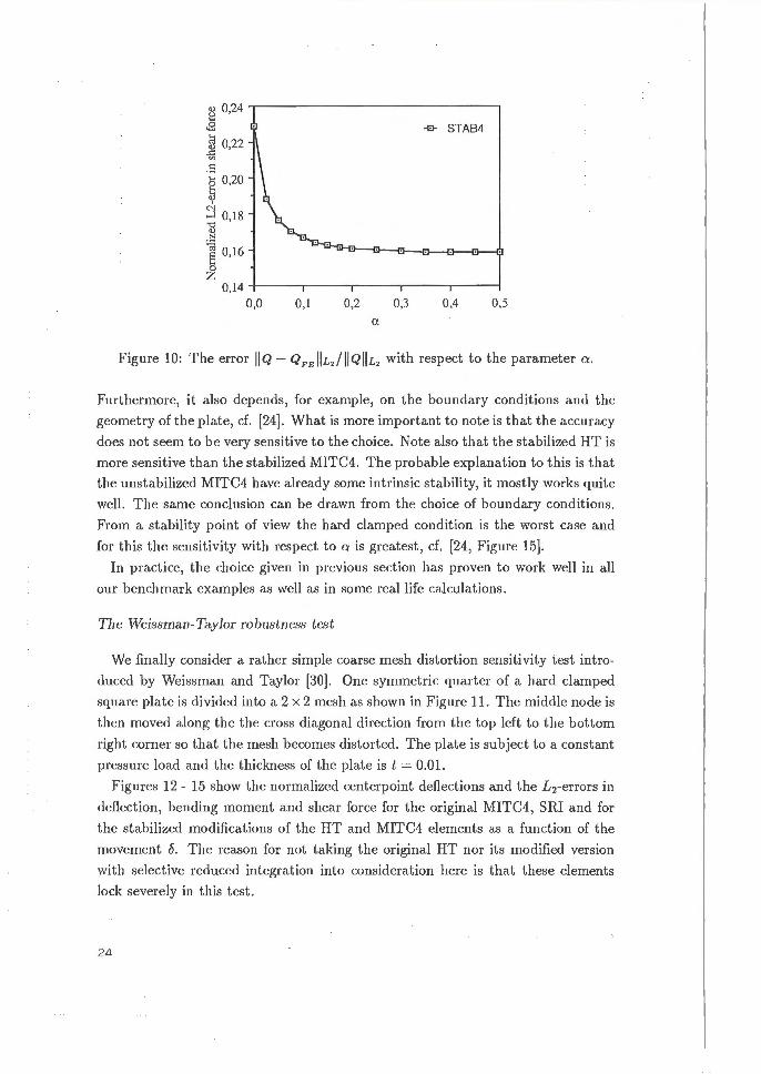
Figure 10: The error IIQ - QFEIIL2 /IIQIIL2 with respect to the parameter a .

Furthermore, it also depends, for example, on the boundary conditions and the

geometry of the plate, cf. [24]. What is more important to note is that the accuracy

does not seem to be very sensitive to the choice. Note also that the stabilized HT is

more sensitive than the stabilized MITC4. The probable explanation to this is that

the unstabilized MITC4 have already some intrinsic stabi lity, it mostly works quite

well. The same conclusion can be drawn from the choice of boundary conditions.

From a stability point of view the hard clamped condit ion is the worst case and

for this the sensitivity with respect to a is greatest, cf. [24 , Figure 15].

In practice, the choice given in previous section has proven to work well in all

our benchmark examples as well as in some real life calculations.

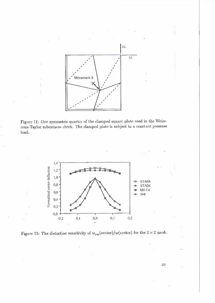
The Weissman- Taylor robustness test

We finally consider a rather simple coarse mesh distortion sensitivity iest intro­

duced by Weissman and Taylor [30] . One symmetric quarter of a hard clamped

square plate is divided into a 2 x 2 mesh as shown in Figure 11. The middle node is

then moved along the the cross diagonal direction from the top left to the bottom

right corner so that the mesh becomes distorted. The plate is subject to a constant

pressure load and the thickness of the plate is t = 0.01.

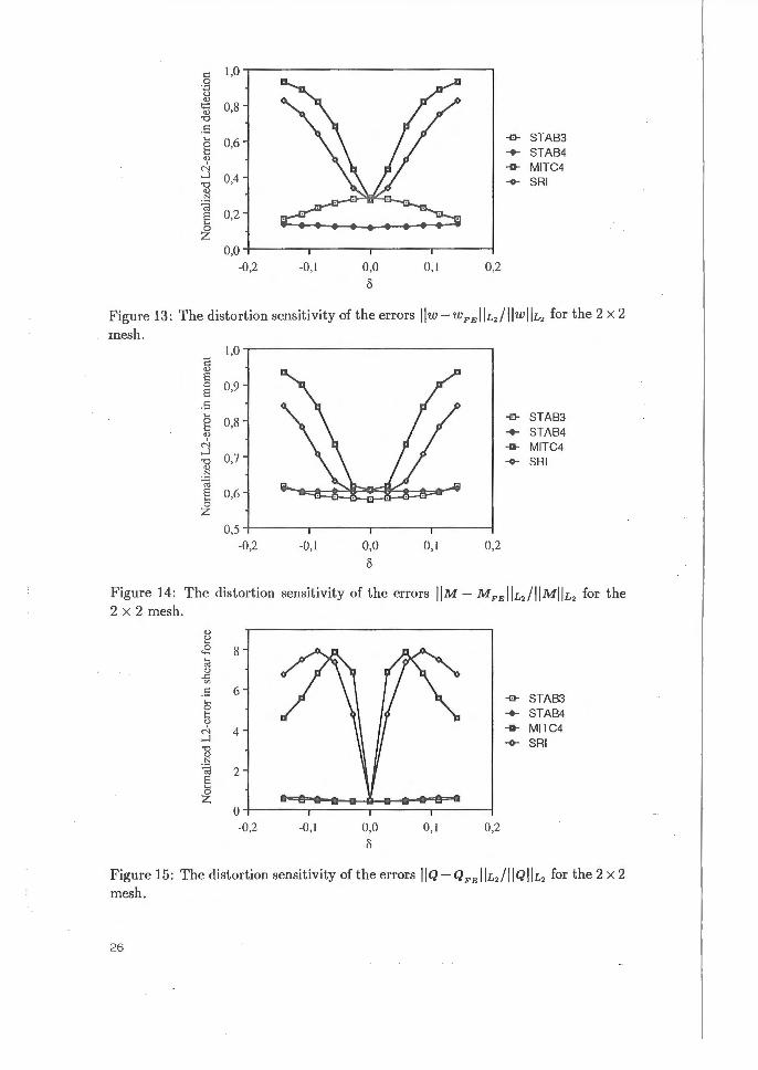
Figures 12- 15 show the normalized centerpoint deflections and the £ 2-errors in

deflection, bending moment and shear force for the original MITC4, SRI and for

the stabilized modifications of the HT and MITC4 elements as a function of the

movement 8. The reason for not taking the original HT nor its modified version

with selective reduced integration into consideration here is that these elements

lock severely in this test.

24

I CL

r,---------~r---------~

/

/

/ /

/ /

/

/

/

/

/ /

I I

I

I I

CL

Figure 11: One symmetric quarter of the clamped square plate used in t he Weiss­man-Taylor robustness check. The clamped plate is subject to a constant pressure

load.

1,4 c:

.S 1,2 u ., z;::

1,0 ., '0 .... "' 0,8 c "'

-e- STAB3 -+- STAB4

(.)

'0 0,6 "' N

-o- MITC4 -o- SRI

;@ 0,4 §

0 ;z: 0,2

-0,0

-0 ,2 -0, 1 0 ,0 0 , 1 0,2

F igure 12: The distortion sensitivity of wFE(center)/w(center) for the 2 X 2 mesh.

25

c: 1,0 .9 u v ..:: 0,8 v "0

.s 6 0,6 -G- STA83 t:: ..... STA84 v 0l -o- MITC4 ...J 0,4 SRI "0 + '-' N :;a

0,2 E .... 0 z

0,0 -0 ,2 -0,1 0 ,0 0 ,1 0 ,2

8

Figure 13: The distortion sensit ivity of the errors llw - wFE IIL2 /IIwiiL2 for the 2 X 2 mesh .

1,0 ;: v E 0 0,9 E

·= .... -G- STA83 g 0,8 v ..... STAB4

c-:. -o- MITC4 ...J "0 0,7 + SRI '-'

. ~ "@ E 0,6 .... 0 z

0,5

-0 ,2 -0,1 0 ,0 0 , 1 0 ,2

8

Figure 14: The distortion sensi t ivity of the errors liM - MFE II£2 /IIMIIL2 for the 2 x 2 mesh.

v ~ ~ 8 @ v

..c: "' ·= 6

STA83 6 -G-

t: ..... STA84 v

c-:. 4 -o- MITC4 ...J + SRI "8 N :;a 2 E .... 0 z

0 -0 ,2 -0,1 0 ,0 0 ,1 0 ,2

R

Figure 15: The distortion sensitivity of the errors IIQ - Q FE IIL2 /IIQIIL2 for the 2 X 2 mesh .

26

As we can see from the figures, the stabilized elements are much more robust

than the others. Especially the shear force of the original MITC4 and SRI elements

is very sensitive for even small changes in 8.

Conclusions

In this paper we have presented stable and optimally convergent three and four

noded Reissner- Mindlin plate elements. By performing some quite extensive nu­

merical tests we have showed that the new elements perform very well and better

than some methods which are well known in the literature. This confers the results

of the mathematical analysis of the methods.

We have tried to do as revealing "benchmark" computations as possible. In the

literature this aspect is far too often treated in a non-satisfactory way. A typical

example would be to calculate a square unit plate with a uniform load and a regular

mesh, and to report on, say, the centerpoint deflection and the maximum moments.

By such a simple test one could, e.g., draw the conclusion that the method with

selective reduced integration is a good method. Our results show , however, that

the method is more or less useless. Instead , we think that in test calculations one

should report on all quantities of physicalinterest for different meshes and loadings,

etc. By doing this we have shown that the possible non-stability of a method is

first seen in an inaccurate and oscillating shear force. That the shear force is a

critical variable appears to be well known (see the remark on page 224 of [20]), but

usually the results for it are not reported. To our knowledge, this problem has not

been addressed until quite recently [23].

To find good benchmark tests is, however, far from a trivial task. We refer to

[6, 4, 5] for some recent interesting discussions on this.

Refe rences

[1] D.N. Arnold and R.S. Falk. Edge effects in the Reissner-Mindlin plate theory. In A.K. Noor, T. Belytschko, and J.C. Simo, editors, Analytical and Computational Models of Shells., pages 71-89, New York , 1989. ASME.

[2] D.N. Arnold and R.S. Falk. A uniformly accurate finite element method for the Reissner-Mindlin plate. SIAM J. Num . Anal., 26:1276- 1290, 1989.

[3] D.N. Arnold and R.S. Falk. Asymptotic analysis of the boundary layer for the Reissner-Mindlin plate model. To appear in SIAM J. Math. Anal.

[4] I. Babuska. The problem of modelling the elastomechanics in engineering. Comp. Meths . Appl. Mech. Engrg, 82:155-182, 1990.

27

[5) I. Babuska and J .T. Oden. Benchmark computation: what is the purpose and meaning? JACM Bulletin, 7( 4):83-84, 1992.

[6) I. Babuska and T. Scapallo. Benchmark computations and performance evaluation for a rhombic plate bending problem. Int. J. Num. Meths. Engng., 28:155- 179, 1989.

[7) K.J . Bathe and F . Brezzi. On the convergence of a four node plate bending element based on Reissner-Mindlin theory. In J . R. Whiteman, editor, The Mathematics of Finite Elements and Applications V. MAFELAP 1984, pages 491- 503. Academic Press, 1985.

[8) K.J. Bathe and F. Brezzi. A simpified analysis of two plate bending elements- the MITC4 and MITC9 elements. In G.N. Pande and J. Middleton , editors, NUMETA 87, Vol. 1, Numerical Techniques for Engineering Analysis and Design. Martinus Nijhoff Publishers, 1987.

[9) K.J . Bathe, F. Brezzi, and S.W. Cho. The MITC7 and MITC9 plate elements. Comput. Struct., 32:797-814, 1989.

[10) K.J. Bathe, M.L. Bucalem, and F. Brezzi. Displacement and stress convergence of our MITC plate bending elements. Eng. Comput., 7:291-302, 1990.

[11) K.J. Bathe and E. Dvorkin. A four node plate bending element based on Mindlin­Reissner plate theory and mixed interpolation. Int. J. Num. Meths. Eng., 21:367-383, 1985.

[1 2) J.-1. Batoz and G. Dhatt. Modelisation des Structures par Element Finis, Vol. 2. Poutres et Plaques. Hermes, Paris, 1990.

[13) F. Brezzi, M. Fortin, and R. Stenberg. Error analysis of mixed-interpolated elements for Reissner-Mindlin plates. Mathematical Models and Methods in Applied Sciences, 1:125-151, 1991.

[14) R.D. Cook, D.S. Malkus, and M.E. Plesha. Concepts and Applications of Finite Element Analysis. John Wiley, 3 edition, 1989.

[15) R. Duran and E. Liberman. On mixed finite element methods for the Reissner­Mindlin plate model. Math. of Camp, 58(198):561- 573, 1992.

[16) L. Franca, R. Stenberg, and T. Vihinen. A nonconforming linear element for Reissner-Mindlin plates. In The Proceedings of the 13th !MAGS World Congress on Computational and Applied Mathematics. Vol. 4. Trinity College, Dublin, Ire ­land, pages 1907- 1908, 1991.

[1 7) L.P. Franca and R. Stenberg. A modification of a low-order Reissner-Mindlin plate bending element. In J. R. Whiteman , editor, The Mathematics of Finite Elements and Applications VII. MAFELAP 1990, pages 425-436 . Academic Press, 1991.

[18) I. Fried and S.K. Yang. Triangular, nine-degrees-of-freedom, C0 plate bending ele· ment of quadratic accuracy. Quart. Appl. Math., 31:303-312, 1973.

[19) T.J .R. Hughes. The Finite Element Method. Linear Static and Dynamic Analysis. Prentice-Hall, 1987.

28

[20] T.J .R. Hughes and L.P. Franca. A mixed finite element formulation for Reissner­Mindlin plate theory: Uniform convergence of all higher-order spaces. Comp. Meths. Appl. Mech. Engrg., 67:223-240, 1988.

[21] T.J.R. Hughes and R. L. Taylor. The linear triangular plate bending element. In J. R. Whiteman, editor, The Mathematics of Finite Elements and Applications IV. MAFELAP 1981, pages 127-142. Academic Press, 1982.

[22] C. Johnson and J. Pitkaranta. Analysis of some mixed finite element methods related to reduced integration. Math. Comput., 38:375- 400, 1982.

[23] D. Lasry and T. Belytschko. Transverse shear oscillations in four-node quadrilateral plate elements. Computers and Structures, 27:393-398, 1987.

[24] M. Lyly, R. Stenberg, and T. Vihinen. A stable bilinear element for Reissner-Mindlin plate model. Comp. Meths. in Appl. Mech. Engrg., 110:343-357, 1993.

[25] M. Mikkola. Levyjen, Laattojen ja Kuorien Teoriaa. Otakustantamo, 1986.

[26] J. Pitkaranta. Analysis of some low-order finite element schemes for Mindlin­Reissner and Kirchhoff plates. Numer. Math., 53:237-254, 1988.

[27] J. Pitkaranta and R. Stenberg. Error bounds for the approJdmation of Stokes prob­lem with bilinear/constant elements on irregular quadrilateral meshes. In J. R. Whiteman, editor, The Mathematics of Finite Elements and Applications V. MAFE­LAP 1984, pages 325-334. Academic Press, 1985.

[28] R. Stenberg. A new finite element formulation for the plate bending problem. Helsinki University of Technology, Laboratory for Strength of Materials. Report 17, 1993. To be published in L. Trabucho, editor, Proceedings of the Jnter·national Con­ference on Asymptotic Methods for Elastic Structures. Lisbon, October 4-8, 1993.

[29] R. Stenberg and T. Vihinen. Calculations with some linear elements for Reissner­Mindlin plates. In P. Ladeveze and O.C. Zienkiewicz, editors, Proceedings of the Eu­ropean Conference on New Advances in Computational Structural Mechanics, pages 505-511, 1991.

[30] S. Weissman and R. Taylor. Resultant fields for mixed plate bending elements. Comp. Meths. Appl. Mech. Engrg., 79:321- 355, 1990.

[31] O.C. Zienkiewicz and R.L. Taylor. The Finite Element Method, 4th edition. Vol I, Basic Formulation and Linear Problems. MacGraw-Hill, 1989.

[32] O.C. Zienkiewicz and R.L. Taylor. The Finite Element Method, 4th edition, Vol II, Solid and Fluid Mechanics, Dynamics and Non-linearity. MacGraw-Hill, 1991.

Mikko Lyly, M.Sc. (Eng.), Rolf Stenberg, Docent

Laboratory for Strength of Materials

Helsinki University of Technology

29