Embed Size (px)
DESCRIPTION
To improve risk management of Road asset
Citation preview
Technical Report AP-T268-14
Application of New Technologies to Improve Risk Management

Application of New Technologies to Improve Risk Management
Prepared By
Freek Faber, Paul Bennett, Wayne Muller, Hanson Ngo
Publisher Austroads Ltd. Level 9, 287 Elizabeth Street Sydney NSW 2000 Australia Phone: +61 2 9264 7088 [email protected] www.austroads.com.au
Project Manager
Renuka Kaul
Abstract
Austroads project AT1539 developed guidance for the use of new technologies that can improve the efficiency of road asset managers. This report is the second stage of the project and it assesses eleven new technologies that can be potentially useful for road asset managers.
Each technology is described in terms of its concepts, physical principles, potential use in asset management and any limitations, case examples and, for level 1 and 2 priority technologies, standards and insights on the costs of the technology. The technologies are mapped to different asset management aspects. This mapping shows the type of data that is collected, which information is obtained and for which asset management aspect this information is used.
Additionally, conclusions are drawn on how to deploy each technology based on the potential use in asset management, market readiness, the quality of the provided data and the costs and business case considerations. In particular, LiDAR technology was assessed to have a significant potential for road asset management. Potential applications and issues have been discussed in dialogue between road agencies and LiDAR industry stakeholders. This resulted in a separate discussion paper describing best practice for mobile LiDAR survey requirements.
About Austroads
Austroads’ purpose is to: • promote improved Australian and New Zealand
transport outcomes • provide expert technical input to national policy
development on road and road transport issues • promote improved practice and capability by
road agencies. • promote consistency in road and road agency
operations.
Austroads membership comprises: • Roads and Maritime Services New South
Wales • Roads Corporation Victoria • Department of Transport and Main Roads
Queensland • Main Roads Western Australia • Department of Planning, Transport and
Infrastructure South Australia • Department of State Growth Tasmania • Department of Transport Northern Territory • Department of Territory and Municipal Services
Australian Capital Territory • Commonwealth Department of Infrastructure
and Regional Development • Australian Local Government Association
• New Zealand Transport Agency.
The success of Austroads is derived from the collaboration of member organisations and others in the road industry. It aims to be the Australasian leader in providing high quality information, advice and fostering research in the road transport sector.
Keywords
Asset management, technology, LiDAR, wireless sensor network, database, new.
Published July 2014 Pages 106
ISBN 978-1-925037-76-0
Austroads Project No. AT1539
Austroads Publication No. AP-T268-14
© Austroads Ltd 2014
This work is copyright. Apart from any use as permitted under the Copyright Act 1968, no part may be reproduced by any process without the prior written permission of Austroads.
This report has been prepared for Austroads as part of its work to promote improved Australian and New Zealand transport outcomes by providing expert technical input on road and road transport issues.
Individual road agencies will determine their response to this report following consideration of their legislative or administrative arrangements, available funding, as well as local circumstances and priorities.
Austroads believes this publication to be correct at the time of printing and does not accept responsibility for any consequences arising from the use of information herein. Readers should rely on their own skill and judgement to apply information to particular issues.
Application of New Technologies to Improve Risk Management
Summary
New technologies play a significant role in asset management and provide opportunities to improve the efficiency of the road asset management task. This project identifies new technologies that are potentially useful for asset managers and for the future development of guidelines for the application of a selection of these technologies.
In particular, LiDAR technology was assessed to have a significant potential for road asset management. The biggest potential is the possibility to reuse LiDAR data for a range of applications from (pre)design to safety to asset inventory. Potential applications and issues have been discussed in dialogue between road agencies and LiDAR industry stakeholders. This resulted in a separate discussion paper describing best practice for mobile LiDAR survey requirements.
However, as new data collection technologies are becoming more affordable, automated and practically applicable, large amounts of new data, called ‘Big Data’ are becoming available for asset management applications. However, many databases and planning software cannot accommodate and use this new data and information. Principles for data management are being discussed in the context of current asset database systems and planning software.
These are two examples of the 11 new technologies addressed in this report. To show which new technologies are suitable for which type of applications, the impact of each technology to the different asset management processes (demand, supply, delivery and operation) is mapped. This mapping shows the type of data that is collected, which information is obtained and where that is used.
This is the final report of Stage 2 of the project. Stage 1 reviewed and prioritised 22 new technologies. Stage 2 provides suggestions for the adoption of each technology based on the potential use in asset management, market readiness, the quality of the provided data and the costs and business case considerations for the 11 most promising new technologies, being:
Top priority technologies:
– 3D imaging of road assets (e.g. LiDAR)
– asset management database and planning software
– wireless sensor network for condition monitoring
Level 2 priority technologies:
– automatic detection of overweight vehicles
– on-board mass monitoring
– non-destructive evaluation technologies for structures
Level 3 priority technologies:
– slope monitoring technology
– ground penetrating radar for pavement assessment
– online origin-destination data collection and travel time estimation
– smart work zone
– roadwork scheduling software.
Austroads 2014 | i

Application of New Technologies to Improve Risk Management
Content
1 Introduction ............................................................................................................................................. 1
2 New Technologies for Asset Management .......................................................................................... 3 2.1 Asset Management Processes ................................................................................................................. 3 2.2 Impacts by New Technologies ................................................................................................................. 4
3 Top Priority Technologies ................................................................................................................... 10 3.1 3D Imaging of Road Assets (e.g. LiDAR) ............................................................................................... 10
3.1.1 Introduction ............................................................................................................................... 10 3.1.2 Description of the Technology .................................................................................................. 10 3.1.3 Physical Principles .................................................................................................................... 12 3.1.4 Use and Limitations .................................................................................................................. 16 3.1.5 Standards ................................................................................................................................. 19 3.1.6 Cost of the Technology ............................................................................................................. 20 3.1.7 Case Examples ........................................................................................................................ 22
3.2 Asset Management Database and Planning Software........................................................................... 24 3.2.1 Introduction ............................................................................................................................... 24 3.2.2 Description of the Technology .................................................................................................. 25 3.2.3 Data Management Principles ................................................................................................... 27 3.2.4 Use and Limitations .................................................................................................................. 29 3.2.5 Costs ......................................................................................................................................... 33 3.2.6 Case Examples ........................................................................................................................ 34
3.3 Wireless Sensor Network (WSN) for Condition Monitoring .................................................................... 35 3.3.1 Introduction ............................................................................................................................... 35 3.3.2 Description of the Technology .................................................................................................. 35 3.3.3 Physical Principles .................................................................................................................... 39 3.3.4 Use and Limitations .................................................................................................................. 39 3.3.5 Standards ................................................................................................................................. 41 3.3.6 Cost of the Technology ............................................................................................................. 43 3.3.7 Case Examples ........................................................................................................................ 44
4 Level 2 Priority Technologies ............................................................................................................. 46 4.1 Automatic Detection of Overweight Vehicles ......................................................................................... 46
4.1.1 Introduction ............................................................................................................................... 46 4.1.2 Description of the Technology .................................................................................................. 46 4.1.3 Physical Principles .................................................................................................................... 48 4.1.4 Use and Limitations .................................................................................................................. 50 4.1.5 Standards and Best Practice .................................................................................................... 51 4.1.6 Cost of the Technology ............................................................................................................. 52 4.1.7 Case Examples ........................................................................................................................ 53
4.2 On-board Mass Monitoring ..................................................................................................................... 55 4.2.1 Introduction ............................................................................................................................... 55 4.2.2 Description of the Technology .................................................................................................. 56 4.2.3 Physical Principles .................................................................................................................... 61 4.2.4 Use and Limitations .................................................................................................................. 62 4.2.5 Standards/Best Practice ........................................................................................................... 66 4.2.6 Cost of the Technology ............................................................................................................. 66 4.2.7 Case Example .......................................................................................................................... 67
Austroads 2014 | ii

Application of New Technologies to Improve Risk Management
4.3 Non-destructive Evaluation .................................................................................................................... 68
4.3.1 Introduction ............................................................................................................................... 68 4.3.2 Description of the Technology .................................................................................................. 70 4.3.3 Physical Principles .................................................................................................................... 71 4.3.4 Use and Limitations .................................................................................................................. 76 4.3.5 Standards/Best Practice ........................................................................................................... 79 4.3.6 Cost of the Technology ............................................................................................................. 80 4.3.7 Case Examples ........................................................................................................................ 81
5 Level 3 Priority Technologies ............................................................................................................. 86 5.1 Slope Monitoring Technology ................................................................................................................. 86
5.1.1 Description of the Technology .................................................................................................. 86 5.1.2 Use and Limitations .................................................................................................................. 86 5.1.3 Case Examples ........................................................................................................................ 86
5.2 Ground Penetrating Radar ..................................................................................................................... 87 5.2.1 Description of the Technology .................................................................................................. 87 5.2.2 Use and Limitations .................................................................................................................. 87 5.2.3 Case Examples ........................................................................................................................ 88
5.3 Origin-destination Data Collection and Travel Time Estimation ............................................................. 88 5.3.1 Description of the Technology .................................................................................................. 88 5.3.2 Use and Limitations .................................................................................................................. 89 5.3.3 Case Examples ........................................................................................................................ 89
5.4 Smart Work Zone ................................................................................................................................... 89 5.4.1 Description of the Technology .................................................................................................. 89 5.4.2 Use and Limitations .................................................................................................................. 90 5.4.3 Case Examples ........................................................................................................................ 90
5.5 Roadwork Scheduling Software ............................................................................................................. 91 5.5.1 Description of the Technology .................................................................................................. 91 5.5.2 Use and Limitations .................................................................................................................. 91 5.5.3 Case Example .......................................................................................................................... 91
6 Discussion and Conclusions .............................................................................................................. 92 6.1 Findings .................................................................................................................................................. 92
6.1.1 3D Imaging ............................................................................................................................... 92 6.1.2 Wireless Sensor Networks ....................................................................................................... 92 6.1.3 Databases and Planning Software ........................................................................................... 92 6.1.4 Non-destructive Evaluation Technologies for Structures ......................................................... 93 6.1.5 Automatic Detection of Overweight Vehicles ........................................................................... 93 6.1.6 On-board Mass Monitoring ....................................................................................................... 93 6.1.7 Findings on Level 3 Priority Technologies ................................................................................ 94
6.2 Discussion .............................................................................................................................................. 94 6.2.1 Potential Use in Asset Management ........................................................................................ 94 6.2.2 Market Readiness and Current Limitations .............................................................................. 95 6.2.3 Quality of the Data .................................................................................................................... 95 6.2.4 Costs and Business Case ........................................................................................................ 96
6.3 Conclusions ............................................................................................................................................ 96 6.3.1 3D Imaging ............................................................................................................................... 96 6.3.2 Wireless Sensor Networks ....................................................................................................... 96 6.3.3 Database and Planning Software ............................................................................................. 97 6.3.4 Non-destructive Evaluation Technologies for Structures ......................................................... 97 6.3.5 Automatic Detection of Overweight Vehicles ........................................................................... 97 6.3.6 On-board Mass Monitoring ....................................................................................................... 97 6.3.7 Conclusions on Level 3 Priority Technologies .......................................................................... 97
6.4 Links to Austroads Guides ..................................................................................................................... 98
References ...................................................................................................................................................... 99
Austroads 2014 | iii

Application of New Technologies to Improve Risk Management
Tables
Table 3.1: Definitions of surveying and mapping grade LiDAR systems ................................................... 12 Table 3.2: Categories of asset management data ..................................................................................... 18 Table 3.3: Cost (US$) for purchasing and operating a 'survey grade' mobile LiDAR ................................ 21 Table 3.4: Operating systems for smart sensors in WSN .......................................................................... 42 Table 4.1: Functional performance requirements for WIM systems ........................................................... 51 Table 4.2: Capture rates and correct read rates for WIM systems ............................................................ 52 Table 4.3: Indicative costs of WIM technologies (for one lane) .................................................................. 52 Table 4.4: Indicative costs for different OBM configurations ...................................................................... 67 Table 4.5: NDE technologies by use .......................................................................................................... 70 Table 4.6: Indicative relative cost of NDE methods for structures ............................................................. 81 Table 5.1: OD and travel time estimation technologies' characteristics ..................................................... 88 Table 6.1: Suggested cross references to Austroads Guides .................................................................... 98
Figures
Figure 1.1: Scope of Stage 2 of the project ................................................................................................... 2 Figure 2.1: From new technologies to asset management decisions ........................................................... 3 Figure 2.2: Mapping top priority technologies to asset management functions ............................................ 5 Figure 2.3: Mapping level 2 priority technologies to asset management functions ....................................... 7 Figure 2.4: Mapping level 3 priority technologies to asset management functions ....................................... 9 Figure 3.1: Available mobile LiDAR systems ............................................................................................... 11 Figure 3.2: Mobile LiDAR system architecture block diagram ..................................................................... 13 Figure 3.3: Photogrammetric principle ......................................................................................................... 14 Figure 3.4: Preferred zones for pointing and measuring ............................................................................. 15 Figure 3.5: Image rectification ..................................................................................................................... 15 Figure 3.6: From data to asset management decisions .............................................................................. 27 Figure 3.7: From data collection to application, examples .......................................................................... 30 Figure 3.8: Multiple potential applications of point cloud data ..................................................................... 32 Figure 3.9: Network-level pavement management ...................................................................................... 34 Figure 3.10: Structural health monitoring system with smart sensors ........................................................... 36 Figure 3.11: Traditional SHM system using centralised data acquisition ...................................................... 36 Figure 3.12: Smart sensor ‘Spec node’ ......................................................................................................... 37 Figure 3.13: Various smart wireless sensor platforms ................................................................................... 38 Figure 3.14: Smart sensor types .................................................................................................................... 41 Figure 3.15: Example of a multiple tiered network topology .......................................................................... 42 Figure 3.16: Wireless standards landscape................................................................................................... 43 Figure 3.17: Strain comparison WSN and reference system ........................................................................ 44 Figure 4.1: Methods for mass monitoring .................................................................................................... 46 Figure 4.2: Piezoelectric cable with quartz crystal sensors ......................................................................... 47 Figure 4.3: A Culway site and Culway II data logger ................................................................................... 48 Figure 4.4: Quartz weigh-in-motion site profile ............................................................................................ 49 Figure 4.5: Auckland Harbour Bridge .......................................................................................................... 53 Figure 4.6: Location Auckland Harbour Bridge WIM and ANPR system ..................................................... 54 Figure 4.7: Number of overweight Auckland Harbour Bridge passes ......................................................... 55 Figure 4.8: Methods for mass monitoring .................................................................................................... 56 Figure 4.9: Methods for on-board mass monitoring ..................................................................................... 57 Figure 4.10: Double-ended shearbeam load cells ......................................................................................... 57 Figure 4.11: Axle load cell fitted to a truck chassis ........................................................................................ 58 Figure 4.12: Fifth wheel load cells on slider bracket ...................................................................................... 58 Figure 4.13: Air pressure transducer connected to an air hose and electrical cable..................................... 59 Figure 4.14: Air pressure transducer system components ............................................................................ 59 Figure 4.15: Six sensor air pressure transducer system ............................................................................... 60 Figure 4.16: Air suspension componentry using square axle beams ............................................................ 60 Figure 4.17: Bluetooth weight indicator ......................................................................................................... 61
Austroads 2014 | iv
Application of New Technologies to Improve Risk Management
Figure 4.18: Silicon membrane and conducting wires in air pressure transducer ......................................... 61 Figure 4.19: The IAP operating model ........................................................................................................... 62 Figure 4.20: A PBS 2B heavy vehicle ............................................................................................................ 68 Figure 4.21: GPR inspection of reinforcement within a precast T-girder ....................................................... 72 Figure 4.22: GPR data showing the position of steel reinforcing bars within concrete ................................. 72 Figure 4.23: Thermographic image of a concrete bridge column .................................................................. 73 Figure 4.24: Trial of gamma-ray gauging to detect defects in timber bridge girders ..................................... 73 Figure 4.25: Example layout of an automated sonar scour monitoring system............................................. 75 Figure 4.26: Microwave interferometry test set-up for bridge monitoring ...................................................... 78 Figure 4.27: GPR inspection of timber girders............................................................................................... 82 Figure 4.28: GPR measurements of deteriorated timber girders .................................................................. 83 Figure 4.29: Trial of UPV for inspecting timber girders .................................................................................. 84 Figure 4.30: Microwave interferometry trial (left) and radar reflector (right) .................................................. 85 Figure 5.1: TSD deflection data and GPR data ........................................................................................... 87 Figure 5.2: Some of the smart work zone system components................................................................... 90
Austroads 2014 | v

Application of New Technologies to Improve Risk Management
1. Introduction
New technologies play a significant role in asset management and provide opportunities to improve the efficiency of the road asset manager. The purposes of this project are to identify new technologies that are potentially useful for asset managers and to develop guidelines for the application of a selection of new technologies for asset/risk management.
This report can be used in two ways:
to identify which new technologies have the biggest potential in improving the efficiency of current asset management processes (biggest return)
to identify potential new solutions for specific asset management tasks.
This is a two-stage project. Stage 1 was completed in FY 2011–12 and covered the gathering of research and information (Austroads 2012a). The result of Stage 1 was the prioritisation and review of 22 new technologies for asset management. Each new technology was briefly assessed and prioritised, into four levels, for consideration by subsequent stages in the project. The first three levels are the subject of Stage 2 of this project, comprising a total of 11 technologies. The remaining level four technologies are of low importance and are not discussed any further in this project.
Stage 2 was undertaken during FY 2012–13 and FY 2013–14 and covered analysis and the development of guidelines for the selected 11 technologies with the biggest potential. They have been described in a sequence of working papers:
Working paper 1 described the technologies rated priority level 3
Working paper 2 described the technologies rated priority level 1
Working paper 3 described the technologies rated priority level 2.
The scope of the project is summarised in Figure 1.1. The information from all working papers has been included in this final report, as well as the input from the two project workshops.
The objectives of this report are as follows:
explore the potential use of these new technologies for asset management, answering questions like what do we own? What is the condition? What is the performance?
identify which technologies might require further inquiry in a later stage.
This report provides a literature review and guidance for the application of the selected eleven highest priority technologies. The scope and depth of the assessment differs by the level of priority.
Austroads 2014 | 1

Application of New Technologies to Improve Risk Management
Figure 1.1: Scope of Stage 2 of the project
For level 1 and level 2 priority technologies, a description of the technology, background of the physical principles, the possible use of the technology in asset management and any limitations, standards, insights on the costs of the technology and case examples are provided.
For level 3 priority technologies, a brief two-page description of the technology, the possible use of the technology in asset management and any limitations and case examples are provided.
Additionally, for 3D imaging technologies (e.g. LiDAR), one of the most promising technologies, a discussion with industry partners has taken place in the form of two workshops. The outcomes have been included in this report.
This report is structured as follows. Chapter 1 introduces the project. Chapter 2 is a reading guide and describes which asset management processes are impacted by which new technologies. Chapter 3 describes the top priority technologies, being 3D imaging of road assets (e.g. LiDAR), Asset management database and planning software and Wireless sensor network (WSN) for condition monitoring. Chapter 4 describes the level 2 priority technologies, being Automatic detection of overweight vehicles, Non-destructive evaluation technologies and On-board mass monitoring. Chapter 5 describes the level 3 priority technologies, being Slope monitoring technology, Ground penetrating radar, Origin-destination data collection and travel time estimation, Smart work zone and Roadwork scheduling software. Chapter 6 includes discussion and conclusions.
Austroads 2014 | 2

Application of New Technologies to Improve Risk Management
2. New Technologies for Asset Management
This chapter explains how the technologies addressed in this document relate to asset management processes and to each other.
It describes the asset management data collection processes and how the new technologies impact data capturing, data processing, information analysis and which asset management aspects are impacted by these technologies.
2.1 Asset Management Processes This section describes how data and information feeds into asset management decisions.
Asset management is based on data and information. Figure 2.1 (to be read from top to bottom) shows how data is captured, stored, processed into information and then fed into asset management decisions. The ovals represent processes. The rectangles represent inputs and outputs. Examples are shown on the left of the figure.
Figure 2.1: From new technologies to asset management decisions
The processes described in Figure 2.1 are driven by the following questions:
Which assets are there?
What is their condition?
How do they perform?
Austroads 2014 | 3

Application of New Technologies to Improve Risk Management
2.2 Impacts by New Technologies This section describes how the new technologies can be used for asset management. It gives an overview of which types of data are captured, which information can be obtained and which asset management functions and processes, covering demand, supply, delivery and operation, are impacted by each technology.
Figure 2.2 show the mapping of the top priority (level 1) technologies, being 3D imaging (e.g. LiDAR), Wireless sensor networks (WSN) and Database and planning software (DBPS). They are mapped to the asset management tasks of data collection, information analysis and asset management decision making.
It shows that:
LiDAR technology captures point cloud data. This data can be used to extract information about bridge clearances, traffic signs and line markings. This information is then used in infrastructure maintenance, provision and renewal, pavement material and bridge technology, road safety, road design and traffic engineering.
Wireless sensor networks capture mainly vibration data which can be used for calculating structural health indicators. These are used for infrastructure maintenance, provision and renewal.
Database and planning software refers to improved storage, processing and analysis of data and information. As several road agencies are currently updating and integrating their asset management database systems, this potentially impacts most aspects of asset management.
This figure shows that developments in both LiDAR and database and planning software have a far greater potential impact than wireless sensor networks.
Austroads 2014 | 4

Application of New Technologies to Improve Risk Management
Figure 2.2: Mapping top priority technologies to asset management functions
Austroads 2014 | 5

Application of New Technologies to Improve Risk Management
Figure 2.3 shows the mapping of the level 2 priority technologies, being non-destructive evaluation technologies (NDE) for structures, on-board mass monitoring (OBM) and automatic detection of overweight vehicles. They are mapped to the asset management processes of data collection, information analysis and asset management decision making.
It shows that:
Non-destructive evaluation technologies are a collection of different technologies using different types of radiation to ‘look’ into structures. Different types of data are captured including mainly reflections and depth profiles. This provides information about the scope and severity of possible problems in structures. This information can be used for decisions on maintenance or network operations in the form of access restrictions for certain types of heavy vehicles.
On-board mass monitoring captures GPS positions and vehicle masses from sensors within (heavy) vehicles. This data provides information about the loads throughout the network and can be combined with mass-based access restrictions for enforcement, mass-based pricing schemes for network operations or by transport operators for transport planning.
Automatic detection of overweight vehicles uses weigh-in-motion technology and number plate recognition cameras to capture pavement strain data and number plates. This provides information about the weight of vehicles at certain locations in the network that can be used to assist enforcement by preselecting potentially overweight vehicles for legal weight checks.
Austroads 2014 | 6

Application of New Technologies to Improve Risk Management
Figure 2.3: Mapping level 2 priority technologies to asset management functions
Austroads 2014 | 7

Application of New Technologies to Improve Risk Management
Figure 2.4 shows the mapping of the level 3 priority technologies, being slope monitoring technology, ground penetrating radar (GPR), origin-destination data collection, smart work zone technology and roadwork scheduling software. They are mapped to the asset management processes of data collection, information analysis and asset management decision making.
It shows that:
Slope monitoring technology captures small movements in slopes. This could provide information about imminent landslides that can be used to warn road workers or road users and improve traffic safety.
Ground penetrating radar captures the thickness profile of the structure of a road, and can help provide input to pavement analysis and pavement maintenance.
Origin-destination collection technologies capture the GPS positions of vehicles. This provides information about the origin and destination of trips and travel demand, which for example can be used for infrastructure maintenance, provisions and renewal planning, and for traffic engineering and traffic modelling.
Smart work zone technology collects vehicle counts and combines this data with information about road works to provide dynamic warnings and routing advice to drivers. This is used for road safety and network operations.
Roadwork scheduling software is used to plan infrastructure maintenance. New algorithms take into account additional cost factors such as travel time costs in comparison with traditional roadwork scheduling algorithms.
Austroads 2014 | 8

Application of New Technologies to Improve Risk Management
Figure 2.4: Mapping level 3 priority technologies to asset management functions
Austroads 2014 | 9

Application of New Technologies to Improve Risk Management
3. Top Priority Technologies
3.1 3D Imaging of Road Assets (e.g. LiDAR)
Introduction 3.1.1The 3D imaging of road assets was identified as the most promising new technology in Stage 1 of this project. For that reason it is specifically scoped in the Contract Note. The priority level 1 technologies are described in terms of:
description of the technology (Section 3.1.2)
background of the physical principles of the technology (Section 3.1.3)
use and limitation of the technology in asset management (Section 3.1.4)
standards and best practice applications (Section 3.1.5)
cost of the technology (Section 3.1.6)
case examples (Section 3.1.7).
For 3D imaging of road assets specifically, a dialogue between road agencies and technology developers and service providers has been facilitated in the form of two workshops with participants from road agencies and from industry. This resulted in a separate discussion paper describing best practice for mobile LiDAR survey requirements.
Description of the Technology 3.1.2This section described the technologies used for three-dimensional imaging (3D) of road assets. 3D imaging of road assets aims to map road assets, including roadside objects such as safety barriers, signage, vegetation and others. The most common technology, LiDAR (Light Detection and Ranging), uses lasers for distance measurement. Another technology is 3D video mapping. This is a special application of traditional photogrammetry, which uses multiple high accuracy video cameras to determine distances (Arcadis 2009). LiDAR can provide more accurate position data, but is generally the more expensive of the two. 3D video mapping uses photographic images, which provides a more natural visual experience to the analyst and user.
LiDAR LiDAR systems are available with different levels of accuracy. They can roughly be classified in two classes, survey grade and mapping grade:
Survey grade is the more accurate type and can record around 1.1 million measurements per second per sensor (3D Laser Mapping n.d.) to 1.6 million points per second (MANDLI n.d.).
Mapping grade is less accurate and records 100 000 pulses per second.
Both types can be applied for different purposes. The possible applications depend also on the travelling speed of the sensing vehicle, and the required level of detail of the 3D image. Section 3.1.4 gives an overview of the possible applications for each type of LiDAR.
The less accurate of these two types of LiDAR is also less complex to build, and consequently less expensive. Section 3.1.6 provides a cost estimate for both types.
LiDAR systems can be used from a fixed base, cars, trains, boats, bicycles or aircraft. 3D monitoring of road assets is generally performed with vehicle mounted LiDAR systems, which are the focus of this study.
Austroads 2014 | 10

Application of New Technologies to Improve Risk Management
Figure 3.1: Available mobile LiDAR systems
Source: Washington State DoT (2011).
LiDAR scanners have made rapid improvement recently. For example, the Optech Lynx LiDAR scanner’s maximum measurement rate has increased from 100 000 points per second to 500 000 points per second. Also its maximum scan rate has increased from 150 Hz to 200 Hz (Optech n.d.). Nevertheless the total system cost remains the same. Other mapping grade LiDAR scanners are available with higher performance and lower cost (Washington State DoT 2011).
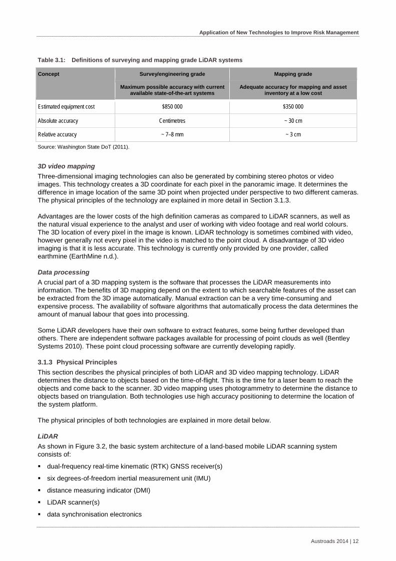
Several mobile LiDAR systems are commercially available for purchase, as contract services, or for rental through their dealers. Figure 3.1 shows several commercially available LiDAR systems during a LiDAR conference. Their cost and performance vary depending on their target applications and configurations. In general, they may be classified into two classes: ‘mapping grade’ systems and ‘survey/engineering grade’ systems. However, some systems can be configured into either class based on the LiDAR scanner(s) and inertial measurement unit (IMU) employed. Mapping grade systems are designed to provide data with adequate accuracy at a low cost for mapping and asset inventory purposes. Typically their absolute and relative accuracy of the data are 30 cm and 3 cm. However, in practice, these systems often achieve higher accuracy, particularly when GNSS signal conditions are good. Their IMU and LiDAR scanner(s) are less accurate than those of the ‘survey/engineer grade’ systems. Many mapping grade systems combine the use of LiDAR scanners and video. A deliberate engineering decision has been made to trade-off performance with cost to provide cost-effective solutions.
Washington State DoT (2011) defines ‘survey/engineering grade’ systems as designed to achieve maximum possible accuracy with current available state-of-the-art GNSS receivers, IMU, digital cameras, and LiDAR scanners (Graefe 2010). These systems produced centimetre-level absolute accuracy data, and could maintain data accuracy with short GNSS signal outage (Frecks 2008, Glennie & Taylor 2008, Graefe 2010, Nobles & Ward 2009, Redstall 2006). In addition, their LiDAR scanners’ range accuracy is 7 to 8 mm. They are designed for survey applications which require the system to deliver highly-accurate and precise data reliably and consistently. Surveying and engineering applications have unique requirements that other applications do not share. Accuracy of the work product carries certain financial and legal liability implications. These systems cost two to five times more than the mapping grade system (Graefe 2010). Table 3.1 gives indicative accuracies and costs of surveying and mapping grade LiDAR systems.
Austroads 2014 | 11
Application of New Technologies to Improve Risk Management
Table 3.1: Definitions of surveying and mapping grade LiDAR systems
Concept Survey/engineering grade Mapping grade
Maximum possible accuracy with current available state-of-the-art systems
Adequate accuracy for mapping and asset inventory at a low cost
Estimated equipment cost $850 000 $350 000
Absolute accuracy Centimetres ~ 30 cm
Relative accuracy ~ 7–8 mm ~ 3 cm
Source: Washington State DoT (2011).
3D video mapping Three-dimensional imaging technologies can also be generated by combining stereo photos or video images. This technology creates a 3D coordinate for each pixel in the panoramic image. It determines the difference in image location of the same 3D point when projected under perspective to two different cameras. The physical principles of the technology are explained in more detail in Section 3.1.3.
Advantages are the lower costs of the high definition cameras as compared to LiDAR scanners, as well as the natural visual experience to the analyst and user of working with video footage and real world colours. The 3D location of every pixel in the image is known. LiDAR technology is sometimes combined with video, however generally not every pixel in the video is matched to the point cloud. A disadvantage of 3D video imaging is that it is less accurate. This technology is currently only provided by one provider, called earthmine (EarthMine n.d.).
Data processing A crucial part of a 3D mapping system is the software that processes the LiDAR measurements into information. The benefits of 3D mapping depend on the extent to which searchable features of the asset can be extracted from the 3D image automatically. Manual extraction can be a very time-consuming and expensive process. The availability of software algorithms that automatically process the data determines the amount of manual labour that goes into processing.
Some LiDAR developers have their own software to extract features, some being further developed than others. There are independent software packages available for processing of point clouds as well (Bentley Systems 2010). These point cloud processing software are currently developing rapidly.
Physical Principles 3.1.3This section describes the physical principles of both LiDAR and 3D video mapping technology. LiDAR determines the distance to objects based on the time-of-flight. This is the time for a laser beam to reach the objects and come back to the scanner. 3D video mapping uses photogrammetry to determine the distance to objects based on triangulation. Both technologies use high accuracy positioning to determine the location of the system platform.
The physical principles of both technologies are explained in more detail below.
LiDAR As shown in Figure 3.2, the basic system architecture of a land-based mobile LiDAR scanning system consists of:
dual-frequency real-time kinematic (RTK) GNSS receiver(s)
six degrees-of-freedom inertial measurement unit (IMU)
distance measuring indicator (DMI)
LiDAR scanner(s)
data synchronisation electronics
Austroads 2014 | 12

Application of New Technologies to Improve Risk Management
data logging computer(s)
digital camera(s).
Figure 3.2: Mobile LiDAR system architecture block diagram
Source: Washington State DoT (2011).
LiDAR scanners for mobile LiDAR systems use either the time-of-flight (TOF) measurement method or phase-based measurement to obtain target point distance (Washington State DoT 2011).
The time-of-flight method works by sending out a laser pulse and observing the time taken for the pulse to reflect from an object and return to the instrument. Advanced high-speed electronics are used to measure the small time difference and compute the range to the target.
LiDAR scanners are capable of measuring up to half a million distances per second. Some LiDAR sensors can detect and provide range measurement for multiple light returns from a single light pulse. This technology enhances the LiDAR sensor’s ability to detect the structure of an object positioned behind vegetation (Washington State DoT 2011).
Phase-based distance measurement works by the phase difference measured between the reflected beam and the transmitted beam. The amplitude of the transmitted beam is modulated continuously. The target distance is proportional to the phase difference and the wavelength of the amplitude modulated signal. Typically, phase-based scanners are capable of achieving a much higher number of point measurements in a second relative to time-of-flight scanners. Their point measurement rate is from about five to one hundred times greater. They do have a shorter useful range, typically 25 to 100 m, where time-of-flight scanners have the technological adaptability to provide longer range, typically between 75 and 1000 m.
Two main photo detector technologies are used in LiDARs. The first is the solid state photo detectors, such as silicon avalanche photodiodes. The second is the photomultipliers. The sensitivity of the receiver is another parameter that has to be balanced in a LiDAR design (Washington State DoT 2011).
LiDAR illuminates the target with laser light and analyses the backscattered light. Additional to measuring the distance based on the time of flight it can also measure other properties such as colour and remission.
Note that remission is reflection of light beams in all directions from non-specular surfaces. It is diffuse reflection. Reflection is the casting back of light which occurs at the boundary surface of two media in accordance with the law of reflection. Reflective objects demonstrate low remission and high gloss. Reflectivity is harder to measure than remission.
Austroads 2014 | 13

Application of New Technologies to Improve Risk Management
LiDAR uses ultraviolet, visible, or near infrared light to image objects, corresponding to wavelengths from about 250 nanometres to about 10 micrometres. A narrow laser beam can be used to map physical features with very high resolution and can be used with a wide range of targets, including non-metallic objects, rocks, rain, chemical compounds, aerosols, clouds and even single molecules (Cracknell & Hayes 2007).
There are two ways in which LiDARs send light pulses. They use either a micro-pulse system or the high energy pulse system. The micro pulse system has been developed as a result of the ever increasing amount of computer power available combined with advances in laser technology. Such systems use considerably less energy in the laser, typically in the order of one micro joule, and are often ‘eye-safe’, meaning they can be used without safety precautions. Road surveying systems use the ‘eye-safe’ micro-pulse system.
3D video mapping As an alternative to using LiDAR technology, 3D mapping can be done using video images. The physical principle used is called photogrammetry. Photogrammetry is used to create a 3D depth map from 2D images. This technology creates a 3-dimensional coordinate for each pixel in the panoramic image. It does that by determining the difference in image location of the same 3D point when projected under perspective to two different cameras. This difference is called disparity. This method of determining depth from disparity is called triangulation (University of Washington 2013). Figure 3.3 shows how the x, y, z position of both cameras are used to determine the position of a traffic sign.
Figure 3.3: Photogrammetric principle
Source: Sistemi Avanzati (2010).
The accuracy of the 3D position depends on the baseline. The baseline is determined by the distance between the cameras, the distance to the object, and the position of the object in relation to the orientation of the cameras. The best results are obtained when the measured object is close to the cameras and in the ranges shown in Figure 3.4.
Austroads 2014 | 14

Application of New Technologies to Improve Risk Management
Figure 3.4: Preferred zones for pointing and measuring
Source: Sistemi Avanzati (2010).
Figure 3.5 shows how an image is corrected for the distortion of the panoramic camera.
Figure 3.5: Image rectification
Source: Sistemi Avanzati (2010).
Positioning Positioning systems, composed of global navigation satellite system (GNSS) receivers, an inertial measurement unit (IMU), and a distance measuring indicator (DMI) are crucial in providing accurate vehicle position and orientation for the mobile system. Performance has significantly improved, and many off-the-shelf positioning systems have recently become affordable.
Austroads 2014 | 15

Application of New Technologies to Improve Risk Management
GNSS receivers determine their location and precise time using time signals transmitted along a line-of-sight by radio from GNSS satellites. Today, there are four GNSS systems (GPS, GLONASS, Galileo, and Compass) in operation or initial deployment phase.
IMUs are composed of accelerometers and gyros. Accelerometers give body acceleration data in three directions, and gyros provide yaw rate (body rotational rate) data in three directions. By integrating this sensor data, the body position and orientation may be calculated at all times.
The accuracy of the final point cloud largely depends on the accuracy of the positioning system of the mobile LiDAR (Washington State DoT 2011).
Use and Limitations 3.1.4Frecks (2012) claims that when measuring bridge heights ‘using this methodology we are able to deliver results in one day instead of one month completing survey projects in a tenth of the time’.
Currently the most common 3D vehicle based imaging technology by far is LiDAR. 3D video mapping technology is mainly used by one surveying provider, earthmine (EarthMine n.d.).
Traditionally surveyors use tripod mounted lasers along the highway to measure features of the road network. LiDAR is currently mostly used on a project level, for instance as a basis for a redesign of a section of road. 3D imaging technology can be used on a project level, but is more and more used on a network level. Typically, on a project level a higher level of detail is needed. A high accuracy LiDAR would be more suitable for this type of application. On a network surveying level, often large distances need to be covered. Low accuracy LiDAR allows for faster measuring speeds and requires less data processing and is therefore more suitable for network surveying tasks.
Additional valuable uses of 3D imaging surveys on a network level that are not directly related to asset management are the reduced need for site visits and the storage of snapshots of the state of the road networks. A lot of the time virtual site visits into the 3D images answer the query. These can be asset management queries (what kind of box is mounted on a light pole?) as well as design or development queries (how much space is there between two objects?). A use that was frequently mentioned during consultation is the use of point clouds as a snapshot in time, e.g. for looking back at the actual situation in case of liability issues.
Possible asset management applications Despite the detailed 3D pictures, point clouds themselves are of limited value for asset management. The real value is in the features of the road and roadside inventory that can be extracted from the point clouds and translated into searchable and meaningful information. A large number of useful features were suggested in consultations with state road agencies and LiDAR service providers:
bridge and tunnel clearance gutters
gantry locations embankments
traffic sign/ITS asset locations reflectivity of lane markings
legal signs (location and sign) signal control locations
street signs/direction signs/advisory signs (location and sign)
gully pits
fauna viaduct dimensions man-holes
vegetation tunnels noise barriers
sight distance clear zones
curvature presence of barriers
lane widths temporary road layouts during road works.
Austroads 2014 | 16
Application of New Technologies to Improve Risk Management
Most of these features are straightforward, however some issues are worth mentioning. The features mentioned during the consultation were a mix of all kinds of data, and are categorised into different types of data in the next section.
Possible applications have been identified from a theoretical perspective. From an overview of different types of data used in asset management (Roberts 2000), the feasibility of detection by LiDAR has been assessed.
A possible application in the field of traffic management is the assessment of temporary road layouts during road works. 3D imaging surveys might be useful to check quickly and efficiently if these road layouts on road work sites meet the requirements.
Types of asset management data Roberts (2000) classified data used in asset management as inventory data and condition data. Inventory data describes the static elements of roads and roadside inventory such as position and dimensions. Condition data describes the condition, which changes over time and needs to be monitored regularly.
Another categorisation is based on the type of asset, distinguishing the road itself and the roadside inventory. The road is the main asset of road agencies that gets traditionally the focus of road asset management, including footpaths, kerbs, civil infrastructures such as overpasses and bridges. The roadside inventory consists of other assets on and around the road such as traffic lights, traffic signs, route signs, gantries, variable message signs and light poles.
The asset management data related to the applications mentioned above are categorised in Table 3.2 by inventory and condition and by road and roadside data.
Currently roadside inventory information is generally entered manually from design drawings upon completion of a (re)construction. Condition information on roadside inventory is collected on site visits and is based on site measurement and images.
Road condition (e.g. rutting, roughness, skid resistance and cracking) is surveyed on a regular basis by other camera and laser based systems with sub-mm accuracies which cannot be realised by current mobile LiDAR systems. Specialised systems are typically used for road condition surveys such as laser profilometers, laser crack measurement systems, ground penetrating radar and travel speed deflectometers.
Data about the condition of roadside inventory is generally not collected, or not in a qualitative way. Roadside inventory is not deteriorating like the road itself. It either breaks, for instance due to an accident in the case of barriers or signs, or is replaced due to reconstruction. Electronic equipment monitoring uses status information communicated by the device itself, rather than using surveys. A possible application however is the monitoring of vegetation.
Austroads 2014 | 17

Application of New Technologies to Improve Risk Management
Table 3.2: Categories of asset management data
Roads Roadside
Inventory Curvature Lane widths Gutters Kerb heights Gully pits Manholes Temporary road layouts during road
works
Bridge and tunnel clearance Fauna viaduct dimensions Traffic sign and other ITS asset
locations Gantry locations Presence of barriers Clear zones Noise barriers Legal signs (location and sign) Street signs/direction signs/advisory
signs Signal control locations Embankments Sight distance
Condition Roughness Rutting Skid resistance Pavement strength Reflectivity of lane markings
Vegetation tunnels
Limitations Some features are easier to extract than others. A current limitation to cost-effective use of 3D imaging technologies is the automatic extraction of features such as bridge heights, traffic signs or clear zones. The automatic detection of features is crucial to realising the benefit of 3D mapping.
The extraction of features is based on the shape of an object in the point cloud. Algorithms to extract features are being developed. To what extent automatic extraction is feasible depends on the exact definition of the feature and the required level of accuracy. For instance, bridge heights may be easily extracted with an accuracy of 10 cm but not so easily with an accuracy of 10 mm. Also, extraction algorithms may be able to succeed in identifying features most of the time, but not always. A success rate of over 80% could be a good performance for some measures but not for others. During the stakeholder consultation the example was mentioned that about 90% of the traffic lights are automatically detected. This requires a person to go through the footage to put in the missing 10%. Additionally it could identify false positives. Again these success rates and performance of these algorithms are being improved quickly. For these reasons it is sometimes not possible to clearly state whether automatic extraction of a feature is possible.
Mobile LiDAR is just one only tool for measuring roads and roadside objects. Although it has many possible applications it may not always be the most suitable or may best be augmented with other scanning technologies such as video, stationary LiDAR or aerial LiDAR.
Other limitations are:
Anything not in the line of sight like culverts, a bridge height when the survey vehicle drives over it, or the earthworks underneath the road surface cannot be detected.
Objects beyond the effective measurement range of the LiDAR system might not be detected accurately. This is generally between 25 and 75 meters. The same range roughly applies to 3D video mapping systems.
Objects that are very small can be missed by the LiDAR beams. Mapping grade systems can have insufficient accuracy for a reliable detection of signs perpendicular to the direction of the LiDAR beams.
Austroads 2014 | 18

Application of New Technologies to Improve Risk Management
Keeping data up-to-date 3D mapping data gets out-of-date as the environment changes. There needs to be a very robust process that ensures that data is recaptured after any modifications or improvements are made to the network. If no systems are in place to ensure that this is undertaken then any database system will soon become out-of-date and consequently not used.
The validity of data over time and the required frequency of data collection differ for the type of information that is obtained. Condition data surveys may need to be done more frequently than inventory assessment surveys. Additionally, it might be useful to annotate the validity of the data when the environment has been modified. This will reduce the risk that decisions are made based on information that is out-of-date.
When assessing the value of 3D imaging system against three main questions in asset management (What do we own? What is the condition? What is the performance?), 3D imaging is able to answer which assets there are, is partly able to answer which condition the assets are in and generally is not able to answer what the performance of the assets is.
Standards 3.1.5Even though 3D mapping technology is still developing rapidly, the need for standards is acknowledged by stakeholders internationally, and first attempts are being made to define best practices and standards for use, uniform reporting of the results and universal data exchange formats. Additionally there are existing standards for asset management data collection that may pose (additional) requirements to asset management application of 3D mapping.
Standards and guidelines for 3D imaging of road assets In line with Austroads national standards for other road condition surveying technologies like the International Roughness Index (IRI) for road roughness, it is expected that national standards will be developed for 3D imaging surveys in Australia. Some of the state road agencies indicated the need to develop these standards in these early days of mobile LiDAR to harmonise best practice and prevent different standards being developed in different states and territories. As a first step towards an Australian and New Zealand standard or guideline this project has drafted a discussion paper describing best practice for mobile LiDAR survey requirements.
In the USA end users and manufacturers agree that standards are needed in the following areas: best practices on the use of mobile LiDAR systems in different applications, uniform result reporting, and universal data exchange formats. These standards will increase the users’ confidence in the performance of their chosen systems, facilitate interoperability, and promote the overall growth of the industry.
The common data format for LiDAR point clouds is the LAS file format. The American Society for Photogrammetry and Remote Sensing (ASPRS) is updating the LAS format to better address requirements for mobile LiDAR mapping application. The ASPRS mobile systems committee is working on a best practices and guidelines documents. In addition, the Geospatial Transportation Mapping Association was formed recently with one of their aims being to create a standard for quantifying results (Washington State DoT 2011).
Requirements posed by asset management standards Washington State DoT (2011) describes three programs that can directly benefit LiDAR, being the ‘Roadside Feature Inventory Programme’, ‘Bridge Clearance Requirements Programme’ and ‘Americans with Disabilities Act’ (sidewalks, driveways, handrails). Standards defined in similar Australian data collection programs could generate requirements for 3D imaging in Australia and New Zealand. Examples of these programs such as AusRAP, iRAP or kiwiRAP, have standards for various risk levels (star ratings) that apply to road design elements as well. All of these are put together using mathematical formulas to form a Star Rating (AusRAP 2006).
Austroads 2014 | 19

Application of New Technologies to Improve Risk Management
Cost of the Technology 3.1.6
Ballpark cost figures The costs of LiDAR surveys can be based on different business models. LiDAR can be bought and operated by road agencies or road agencies can hire the services of survey providers to do the surveys, data processing and information extraction for them.
Costs can be broken down into three categories:
1. information technology (IT) costs
2. data collection costs (including hardware, processing, maintenance and operational costs)
3. data extraction costs (labour costs for extracting data).
Information Technology costs consist of storage, servers, backup, data extraction software and workstations for data extractions. The IT cost estimate from the Washington State DoT (2011) cost benefit analysis pilot is for:
storage at about US$22 per mile. This is based on 3 GB per mile and a charge of US$7.3 per gigabyte storage by Washington State DoT IT department
five new workstations for data post-processing are estimated at five times US$3000 each, total cost is US$15 000
data extraction software licences and yearly renewal costs are $80 000 and $20 000 per year.
A ballpark figure for LiDAR data collection costs by a survey provider is about A$100 per kilometre, which is in the same ballpark as the US$40 to US$85 per kilometre estimated by Washington State DoT (2011). These figures are examples for surveys of short sections of road.
For network wide surveys, the hire of a survey grade system including vehicle and driver would cost A$2000 to A$10 000 per day.
Data extraction costs are the total cost of the personnel to extract features such as dimension and position of objects. The data extraction cost depends highly on the number of features required to be extracted, and the level of automation of the extraction. Even highly automated feature extraction generally has an accuracy of 80% depending on the feature. This means that human checks and correction are required.
The Washington State DoT pilot cost benefits analysis assumes 1.5 labour hours per kilometre for the extraction of the required geospatial data for the three Washington State DoT data collection programs covered by this pilot. The required geospatial data includes more than 20 roadside features including kerbs, sidewalk ramps, sidewalks, crosswalks, driveways, island and median cut-throughs, signal type and location, shared use paths, handrails, culverts, signs and objects in clear zones (Washington State DoT 2011).
Table 3.3 shows a cost estimate example (in US$) for purchasing and operating a 'survey grade' mobile LiDAR system. The Washington State DoT cost estimates are based on collecting data for Washington State with contains more than 7000 freeway miles, and assumes about 15 000 miles need to be driven to cover that (roads are measured once in each direction at the minimum). To simplify calculation, it was further assumed a uniform labour rate of US$50 per hour for all of the personnel needed for data collection and processing (Washington State DoT 2011).
Austroads 2014 | 20

Application of New Technologies to Improve Risk Management
Table 3.3: Cost (US$) for purchasing and operating a 'survey grade' mobile LiDAR
Description Year 1 and 2 1st cycle
($)
Year 3 and 4 2nd cycle
($)
Year 5 and 6 3rd cycle
($)
Total 6 yrs 3 cycles
($)
IT data storage cost 328 500 328 500 328 500 985 500
IT server cost 1 000 0 0 1 000
Data post-processing workstations (5 at $3 000 each)
15 000 0 0 15 000
Data extraction software 80 000 0 0 80 000
Data extraction software maintenance 20 000 40 000 40 000 100 000
Total IT cost 444 500 368 500 368 500 1 181 500
Survey grade mobile LiDAR equipment cost 850 000 0 0 850 000
Survey grade mobile LiDAR equipment maintenance cost (10% equipment cost per year)
85 000 170 000 170 000 425 000
Training 50 000 0 0 50 000
Vehicle cost (6 months/year, = $700/month x 12 months)
8 400 8 400 8 400 25 200
Personnel cost ($8 650/month, 3 person crew for 6 months)
311 400 311 400 311 400 934 200
Total data collection cost 1 304 800 489 800 489 800 2 284 400
Data extraction cost (3 hr/mi for 1st cycle, 1.5 hr/mi for subsequent cycle, @ $50/hr)
150 75 75
Total data extraction cost 2 250 000 1 125 000 1 125 000 4 500 000
Total cost 3 999 300 1 983 300 1 983 300 7 965 900 Source: Washington State DoT (2011).
Building a business case The business case for using LiDAR technology in asset management is more than just the cost of the technology itself. It includes processing costs and operating costs, and benefits. In the cost benefit analysis of seven mobile LiDAR deployment options by the Washington State DoT (2011) half or more of the cost was the data extraction cost.
Based on consultations with road agencies and industry in Australia, the most common business model for road agencies is to outsource the surveying, the data processing and the data extraction to a survey service provider.
The main reasons are the high level of specialised expertise that is required which is expensive and not feasible to provide in-house and the rapid developments making in-house knowledge out-of-date quickly.
Washington State DoT (2011) compared contracting for mobile LiDAR services with purchasing a mobile LiDAR system and renting one. They calculated that purchase options have lower lifecycle costs and produce larger saving than the rental options, although the costs for the different options are similar. This is based on the assumption that there are about 24 000 kilometres that would need to be driven by the data collection vehicle in order to pick up both directions of the more than 11 000 highway kilometres of Federal and State of Washington highways and freeways managed by Washington State DoT. For comparison, VicRoads manages 22 400 kilometres of freeways and arterial roads (VicRoads 2013).
Austroads 2014 | 21

Application of New Technologies to Improve Risk Management
To complete the business case picture, the benefits need to be addressed as well. Two types of benefits can be distinguished.
1. A more efficient way to undertake current processes (e.g. cheaper data collection)
2. New information allowing for better performance or outcomes (e.g. fewer trucks crashing into bridges).
Benefits of 3D mapping are generally cost savings in the data collection processes. LiDAR has possible applications in many areas such as safety, infrastructure maintenance planning, and road design. A combined data collection effort between different departments might require coordination between departments, but would result in a positive business case. Therefore, to complete the business case costs of data collection using the current technologies need to be included from different departments. This is however not in the scope of the project brief.
Intangible benefits Additional to the hard benefits calculated in a business case, data collection using LiDAR could have intangible benefits, which could be larger than the tangible benefits. Mobile LiDAR technology reduces the amount of labour, vehicles, and carbon dioxide emissions required for data collection. In addition it increases the speed of data collection and reduces time to acquire the critical geospatial data required for making policy decisions. Delay between data requested and data provided is often the invisible cause of project delays. The major intangible benefactors are often other agencies or departments not knowing of the potential use of point cloud data in their processes, such as preconstruction engineering teams, those who design roads, bridges, and other infrastructure. There are many untapped potential applications of point cloud data that can be explored.
Case Examples 3.1.7Case examples collected during the consultations with the stakeholders are briefly described here. There are many other examples of mobile LiDAR projects in Australia and across the world.
Examples of mobile LiDAR applications include:
MRWA project using the StreetMapper product
UK Highways Agency
Utah Department of Transportation
Washington State DoT pilot
earthmine pilot in Western Australia
Queensland LiDAR surveys
Sydney Harbour Bridge modelling
City of Newcastle – City Precinct 3D Modelling.
MRWA project using the StreetMapper product In 2011 a survey along the North West Coastal Highway in Western Australia was completed using StreetMapper, a vehicle-based laser mapping system. Travelling at normal traffic speeds, the StreetMapper system captured survey grade data achieving millimetre accurate measurements of the road surface and roadside features. StreetMapper mobile surveys replace the need for surveyors using tripod mounted lasers along the highway making it a much faster and safer process, as well as reducing disruption for other road users.
Commissioned by Main Roads Western Australia (MRWA), the laser scan survey was requested by consulting surveyors Hille Thompson and Delfos. The survey route included a section of the main highway, which forms part of the coastal link between Perth and Port Hedland, via Geraldton and included offsets from the highway along intersecting roads.
Austroads 2014 | 22
Application of New Technologies to Improve Risk Management
Hille Thompson and Delfos were already part way through the project – having to engage third party traffic management and work at night to avoid conflicts with other road users – when they became aware that the StreetMapper system was in Western Australia. Having seen the system in operation in Perth, the company realised they had a window of opportunity to test StreetMapper on a real project while saving thousands of dollars, not to mention innumerable headaches, in out-of-hours working and traffic management.
The StreetMapper system completed the 8.5 km survey of the main highway plus intersecting roads in a matter of hours, without any real disruption to other road users and during normal working hours. The verified and rectified point cloud was then processed by Hille Thompson and Delfos to extract information about road and roadside features in conformance with MRWA’s requirements (StreetMapper 2011).
UK Highway Agency pilot In November 2012 Bentley Systems was challenged by the UK Highways Agency to come up with a solution for managing their LiDAR data over the entire strategic network. The solution proposed to the UK Highways Agency during February 2013, highlighted key elements such as linear referencing and spatial data management capabilities coupled with document management capabilities and a tool which was used for basic interrogation and analysis of the raw LiDAR data.
All documents relating to the LiDAR survey section are associated to the asset through the Exor Document Management system with all documents containing high and low resolution fly-through movies, snapshot images of the LiDAR field of view, photographs of the field of view and the raw LiDAR data itself. Each document type is visualised in the map view using specific symbols and themes to distinguish between them. Documents are located at the same location of the LiDAR survey section. This case was described by Dave Body, Solution Executive – Roads and Bridges at Bentley Systems in an email and a phone conversation in February 2013.
Utah DoT roadway imaging/asset inventory project Utah Department of Transportation is employing LiDAR to improved asset management. Mandli Communications was contracted to gather, identify, and process a wide variety of roadway assets along its entire 6000-plus centre lane miles of State routes and interstates.
The initially small Utah DoT team began to see that there was more potential to their efforts than just pavement distress data. By asking ‘What data can your division use to enhance your asset management decisions through a simplified collection effort?’ it was discovered that some divisions had been duplicating efforts and quickly a dynamic and diverse team began to form.
The Utah DoT Roadway Imaging and Inventory program requires the vendor to gather several different roadway assets including roadway distress data, surface areas, lane miles, number of signs, vertical clearances, and more.
Sensors on the Mandli vehicle used in Utah include a Velodyne LiDAR sensor, a laser road imaging system, a laser rut measurement system, a laser crack measurement system, a road surface profiler, and a position orientation system (Ellsworth 2013).
Washington State DoT pilot Washington State DoT completed a field study comparing mobile LiDAR from different providers. This included references to other examples of the use of LiDAR amongst US DoTs. Private contractors and service providers have been using mobile LiDAR extensively to collect geospatial data for mapping, asset management, and survey. A few state DoTs, such as Tennessee DoT, Hawaii DoT, Nevada DoT, and Texas DoT, have contracted with mobile LiDAR service providers for asset management. Caltrans has contracted with a mobile LiDAR survey firm to perform bridge clearance measurements and pavement surveys. Recently, Oregon DoT has purchased a mapping grade mobile LiDAR system. Survey service providers have been using survey grade mobile LiDAR systems to collect data for railroad and power transmission line management (Washington State DoT 2011).
Austroads 2014 | 23

Application of New Technologies to Improve Risk Management
Based on their cost-benefit study, Washington State DoT (2011) recommends the option of purchasing and operating a mobile LiDAR system because it generates savings and meets most Washington State DoT business requirements. Also the number of survey grade mobile LiDAR systems available for rental in the US was quite limited. However, they state that renting and operating a mobile LiDAR system should be considered if the equipment utilisation rate is low or if a lower initial cost is required for lack of funds.
3.2 Asset Management Database and Planning Software
Introduction 3.2.1This section is about how asset management databases and planning software (DBPS) can incorporate new types of data and information from new data collection technologies like LiDAR and wireless sensor networks.
DBPS are also called road infrastructure management systems. These systems are developed for one or more of the following purposes:
reporting on the network (to government and the public at large)
developing policies and standards
network planning for maintenance of the existing infrastructure, and for new works
determination of budgets for financing of the network
development of works programs for undertaking maintenance and new works, including identifying the type of treatment or new works for each management section
feedback on performance of works to the developing of policy, standards, and designs.
Examples of a frequently used combination of database and planning software are the RAMM (Road Assessment and Maintenance Management) database and dTIMS planning software, used in all of New Zealand, and in Western Australia where they were implemented as part of the ROMAN II project.
Even though asset management databases and planning software play a crucial role in the asset management processes, they are not a new technology. The reason that they are assessed here as a level 1 priority ‘new technology’ is that the data that is available has changed. Developments in data collection technologies make large amounts of data available for analysis and planning, called Big Data. The asset management databases and planning software is the key to making use of Big Data for more efficient asset management. In the context of asset management Big Data refers for example to survey data from laser crack measurement systems, travel speed deflectometers, LiDAR point clouds, and video or structural health data from WSN.
Questions about the expected benefits of Big Data, how this will affect the planning of maintenance and how the next generation of scalable database and planning software should be supported cannot be answered in this project. The scope of this analysis of DBPS is defined as:
identifying scalability issues of DBPS
drafting scalability principles for DBPS
identifying directions for solutions to scalability issues (cloud computing, data mining).
Apart from these new challenges, a current challenge is to keep database systems up to date. Database systems get out-of-date as the environment changes. There needs to be a very robust process that ensures that data is recaptured after any modifications or improvements are made to the network.
Austroads 2014 | 24

Application of New Technologies to Improve Risk Management
Description of the Technology 3.2.2Databases and planning software are often used as a combination as they need to be interoperable. They are however two separate systems. Frequently used solutions are described as well as the historical perspective to the requirements of road information management systems.
Current practice DBPS are widely used throughout Australia and the rest of the world. The following DBPS or ‘asset management systems’ are commonly used in Australia and New Zealand. This is not an exhaustive list, but serves as an example of the scope and status of contemporary practice.
Road asset database systems RAMM (Road Assessment and Maintenance Management) is used as the database under the ROMAN II
software package that is installed in a number of WA councils and in NZ (see Section 3.2.6 for case study examples).
IRIS is used by MRWA. All asset management information is gathered there and is accessible for different departments.
Planning software dTIMS is used as the planning software in the ROMAN II software package (see Section 3.2.6 for case
study examples).
HDM-4 is a dedicated road network decision support tool with comprehensive models for all aspects of road and vehicle operation (HDM Global 2013).
SMEC Road Asset Management System is adapted from HDM technology (SMEC n.d.).
Huefner Management Systems (Huefner Management Systems n.d.).
The following issues have been raised during stakeholder consultations with state road agencies when discussing the current practice of asset management databases and planning systems in the context of LiDAR use:
Generally with most database systems, processed data (or information) is being stored separately from the detailed raw data such as point clouds. The raw data is often stored by the survey provider.
These traditional asset management systems are used for storing road and pavement condition data and developing maintenance and renewal strategies.
However, for other off-road data within the road reserve, referred to as ‘roadside’ inventory data, this is often collected in separate systems and on an ad hoc basis. Currently several jurisdictions are making efforts to integrate their different database systems.
The storage and processing of large amounts of data from surveys such as video or LiDAR point clouds is often outsourced to survey service providers and made available through web interfaces and cloud computing.
A historic perspective A road asset management system is a software product that manages and analyses various road data to assist in decision-making regarding the maintenance of roads and other related assets. Asset management systems are used for the following: interpretation of road condition data, identification of optimal treatments, calculation of life-cycle costs, the development of programs of work and the prioritisation of maintenance treatments. Road infrastructure includes the whole road related network and its assets, the pavements, all structures (bridges, tunnels etc.) and off-pavement assets such as drainage, signs etc.
Roberts (2000) provides a historic perspective to road asset management systems. Historically road asset information management systems have evolved into databases and planning software. It is possible to visualise database and planning software as being produced as a series of generations, as defined below. The use of the term generation is very convenient for describing the development through time of the philosophy and technology of these systems.
Austroads 2014 | 25

Application of New Technologies to Improve Risk Management
First generation A paper or index card based road infrastructure asset management system, in which the main considerations were minimising agency costs to meet a certain minimum standard.
Second generation A computerised road infrastructure asset management system, with limited condition prediction capability (one or two years), in which the main considerations were again minimising agency costs to meet a certain minimum standard.
Third generation A computerised road infrastructure asset management system, with significant forward condition prediction capability (10 years and more), which takes account of agency and road user costs in a benefit cost, life-cycle analysis, and in which decisions are driven by economic performance.
Fourth generation A computerised road infrastructure asset management system, with significant forward condition prediction capability (10 years and more), which takes account of not just agency and road user costs in a benefit cost, life-cycle analysis, but also other factors in a multi-criteria analysis. These systems are often also associated with GIS (Geographical Information System) databases, and GPS (Global Positioning System) technology for locational referencing of data. Data is mainly collected at highway speed using objective automated means.
A fifth generation of databases and planning software is emerging. Whereas the fourth generation uses a combination of traditional data and data capturing technologies, the current objective is to collect data at highway speeds. The fifth generation takes full advantage of closely-spaced machine-captured Big Data, and operates as a fully integrated system including all fence to fence asset management data and information.
In this outline of such software systems, a number of desirable and required features need to be considered, including the following:
functionality in data presentation, with characteristics of direct relevance for roads such as well-designed linear strip maps of each road link
automatic linkages in real time to commercial database software
automatic linkages in real time to commercial GIS mapping presentation software
either a full suite of integral hard coded good mathematical models for use in data analysis (with variables directly associated with condition and performance parameters of the roads), with sufficient control for their adjustment and calibration
or the capability to code in mathematical models selected by the user with full control by the user for model editing and configuration etc. (without need to refer to the software supplier)
integral and satisfactory procedures for the optimisation of outputs from the main data analysis stages (for example the selection of the optimal project option), or the capability to link with external optimisation software packages
pre-selected and acceptable systems for data reporting through graphs, charts and mapping presentations, or the scope for the development of external presentations by export of data into separate software
integral systems for the management of road infrastructure works at the implementation stage.
A number of road data collection technologies have been implemented or are being considered. A wealth of data and information is becoming more readily available. One of the challenges is the interpretation and analysis of the data to assist decision-making. Asset management databases and software are necessary to maximise the benefits from road data collection technologies.
Austroads 2014 | 26

Application of New Technologies to Improve Risk Management
Data Management Principles 3.2.3This section describes asset data management.
From data to decisions Data about the state of the roads is collected to support planning and decisions about maintenance. Figure 3.6 describes how data is captured, processed and analysed for policy or operational decisions. The ovals in the figure describe processes; the rectangles describe the outcome of a process. Some examples of the outcomes are shown on the left side of the figure.
Data collection technologies are evolving rapidly. The next steps in the process, data processing, storage and analysis will have to keep up with the capture of huge amounts of data, Big Data, by the new data collection technologies.
Figure 3.6: From data to asset management decisions
Examples of Big Data collection technologies are LiDAR, video, the travel speed deflectometer and wireless sensor networks. These new types of data are an opportunity for asset management. The opportunity is threefold:
1. Current processes can be done more efficiently. For example, measuring offsets and distances using a point cloud is much faster than if someone has to physically visit a site to measure these distances using traditional survey equipment. Also, the application of a wireless sensor network system to measure the structural health of a bridge is less complex than the installation of large networks of traditional wiring circuitry.
2. New data allows for new applications. For example, performance based standards for access of heavy vehicles could be applied automatically based on 3D images of the road. Video surveys could be used to analyse the reflectivity of line markings so that periodical repainting of line markings can be postponed until necessary. The potential of new applications is difficult to predict because, innovation in system-use tends to build on the original innovation itself, through usage of the system.
3. Data can be used for several aspects of asset management, including safety, traffic modelling, project preparation and implementation and road design.
Austroads 2014 | 27

Application of New Technologies to Improve Risk Management
For new data collection technologies, generally the survey providers take over a number of the processes from the asset manager. These survey service providers process and store the large amounts of data collected by LiDAR, video or TSD, with just the processed information being used by the asset manager. However, as familiarity increases with the new Big Data and its applicability, the asset manager is likely to wish to have more control of the raw data than is currently expected in these first stages of the deployment of such Big Data technologies.
Guiding principles Australian Local Government Association and ANZLIC, the Spatial Information Council (2007) have developed a local government spatial information management toolkit, which summarises general guiding principles for data management as follows:
do not reinvent the wheel – identify leading practice and implement it
where possible, capture data once and use it for multiple and/or generic purposes
avoid duplication in data acquisition
use existing systems and/or facilities wherever possible
manage data to maximise their value both during and after the project for which they were collected – design for long data life
give priority to the broadest value data – that is, data that has benefits for multiple processes and multiple users
develop long-term strategic goals for data and information management that also align to organisational needs
select the most robust organisation with the broadest span of interest to be the most appropriate custodian of high-value general-use information
reinforce and support data custodians and negotiate protocols for data access
develop and enforce data documentation and metadata standards and approaches.
The italic highlighted principles are especially relevant to the challenge of incorporating new data from new technologies.
The use of existing systems and facilities is encouraged. The existing systems are the traditional road condition surveying technologies such as laser profilers, road condition databases and maintenance strategy planning software. New technologies, data and processing algorithms should preferably be integrated with these existing systems.
The design for long life data relates to the question of whether to store raw data for later use. A case-by-case decision has to be made on whether raw data, processed data or both are stored. This decision should influence the data collection design to provide the feedback for a proper design for long data life.
To assess the value of new data from new data collection technologies the concepts of the broadest value data should be applied. Section 3.2.4 about the use and limitation of data outlines an example of multiple applications of LiDAR data by multiple stakeholders.
The strategic goals for data and information management, aligned with organisational needs, are important for the decision to adopt new technologies in data collection programs. Section 3.2.4 describes different asset management applications, and some of the information and data needs.
Currently different departments are often responsible for their own data collection. Safety related data collection is different from road condition data collection. Some of the road agencies are making efforts to coordinate data collection and organise custodianship centrally. A data custodian is an appointed group or position that is, by the owner of the data, made responsible and accountable for the management and care of the data holdings under their control, in line with the defined data policy.
Austroads 2014 | 28
Application of New Technologies to Improve Risk Management
Big Data and data mining In the context of asset management Big Data refers for example to survey data from laser crack measurement systems, travel speed deflectometers, LiDAR point clouds, and video or structural health data from WSN.
There is added value if these data sources can be used to answer questions in a more efficient way. The biggest benefit however is when the data can be used to gain new insights. ‘Data mining’ techniques are available to combine information from different datasets and discover something new. Fayyad et al. (1996) defined data mining as the analysis step of the knowledge discovery in databases. For example matching road condition data with crash statistics can provide new safety criteria for road resurfacing policies.
An issue for big data is the geographical location relationship between the various datasets. The key requirement to successfully linking geographically referenced data sets is to ensure a common location referencing standard. For example when integrating various data sets on the condition of the pavement, data sets including profilometer data and surface ratings could be combined. However this is only possible with coordination of the data location of the different data sets. To get maximum benefits from big data the geographical location is critical.
Use and Limitations 3.2.4This section describes the use and limitations of database systems and planning software. It gives an example of how the proposed framework in Section 2.1 and the ‘guiding principles’ described above can be used to identify opportunities for the use of new Big Data and for identifying technologies that might become redundant.
Limitations of data collection and usage Figure 3.7 shows the process of data collection and usage for policy and operational decisions for different functions of asset management. It shows examples of the technologies that are currently being used, including relatively new technologies. It shows examples of the raw data that is being collected, and of the information that is extracted from this data, and aspects of asset management for which decisions will be made (partly) based on data. The figure gives common examples but is not an exhaustive list.
Austroads 2014 | 29

Application of New Technologies to Improve Risk Management
Figure 3.7: From data collection to application, examples
Austroads 2014 | 30

Application of New Technologies to Improve Risk Management
The database systems and planning software that facilitate this process are depicted in the arrows. Some of the important elements of the data collection are the required storage capacity of the database systems and the processing capabilities of the data collection systems. Processing of data during data collection reduces the need for large data to be stored and enables useable information to be readily available without post-processing.
To translate data into information, standards and algorithms are crucial for consistent and commonly agreed (international) indicators. Finally (planning) software provides input to decisions on maintenance, road safety measures or road design based on models.
Not all facilities are in place for the new technologies to provide useful input to decision making. During stakeholder consultations it was found that data storage and access in jurisdictions have limitations in dealing with large amounts of data. Current standards do not allow easy cross-referencing between aspects of asset management. For example, standards for point clouds are not present which makes the reliable automatic extraction of information by third party algorithms difficult. The result of this is that the capabilities of planning software to convert data into useful information for decision making are largely untapped.
When assessing the value of DBPS against three main questions in asset management (What do we own? What is the condition? What is the performance?), the result depends on the scope of DBPS. DBPS are generally able to answer which assets there are, they are generally able to answer which conditions the assets are in and they are able to answer what the performance of the assets is.
Multiple applications of point cloud data This section gives an example of how Figure 3.7 can be used to identify opportunities for the use of new Big Data and identifying technologies that might become redundant.
By identifying the links between the technologies, the data that they can collect, the information that can be obtained from this data, and the decisions that can be made based on that data, the value of the data can be determined.
Figure 3.8 shows how point cloud data can potentially have multiple applications in different functions of asset management. Bridge heights could be used for safety measures and heavy vehicle access. Traffic sign information could be used for safety measures and traffic engineering, and line markings could be used for maintenance planning and road design.
Austroads 2014 | 31

Application of New Technologies to Improve Risk Management
Figure 3.8: Multiple potential applications of point cloud data
Austroads 2014 | 32

Application of New Technologies to Improve Risk Management
By doing this analysis for other technologies and comparing the input of the technology to the actual decision making, the value of new data collection technologies and existing technologies can be compared.
This can be used to see how data management can be improved by identifying the trends, identifying the relationships between the collected data and the applications/decisions, identifying the implications of the trends, and thus identifying opportunities for the use of new Big Data and identifying technologies that might become redundant.
Comparing the value of different new technologies and the implications from database and planning software that are currently used by jurisdictions is a big task. It requires obtaining a clear understanding of the developments in data collection technologies, as provided in this study. It also requires an understanding of the value of the new data sources in asset management. These understandings need to be operationalised into useful assessment criteria, and confirmed by stakeholders. Finally the assessment needs to be performed and evaluated with the stakeholders.
Costs 3.2.5This section gives a ballpark estimate for the costs of database and planning software for asset management. Additionally there are costs for data collection; however they are not addressed here. The cost at issue is related to the costs of data collection. Because of the specific knowledge that is needed for processing of certain types of data, data processing and storage are offered as a service with data collection. The considerations of in-house data storage and processing versus outsourcing of data storage and processing are not addressed. This section only provides examples of costs for the following cost components of database and planning software:
data storage
data processing
software
labour costs.
Data storage The Washington Department of Transportation (2011) business case study on LiDAR uses A$7 per year per gigabyte storage by the Washington State DoT IT department. Based on 3 GB of point cloud data per mile this is about A$20 per mile. Cloud computing service providers offer data storage for about A$0.125 to 0.15 per GB per month which would be about A$5 per GB per km on point cloud data.
Data processing The costs for data processing depend on the required calculation tasks. The Washington Department of Transportation (2011) business case study assumes it needs five new workstations for data post-processing for the 7000 miles of freeway network. The workstations are estimated at five times A$3000 each, total cost is A$15 000. Processing intensive tasks like data mining might even require more expensive hardware.
Software Software costs can vary substantially as well. Database and planning software are sold as a package or as separate components. Prices vary from about A$10 000 for simple systems with database and current status work programs functionality to about A$50 000 for systems with predictive modelling and life cycle costing functionality. The price depends amongst others on how many criteria need to be assessed and how much the data formats need to be modified. A fully integrated asset management system including buildings, drainage, parks, etc., can cost up to several hundred thousands of dollars.
Labour costs Labour costs largely depend on the extent to which data processing, running of models and performing analyses with the software are automated. Especially for new technologies the level of automation might not be as high as for existing systems. Additionally there may be setup costs or costs associated with the integration of new data or information into existing systems.
Austroads 2014 | 33
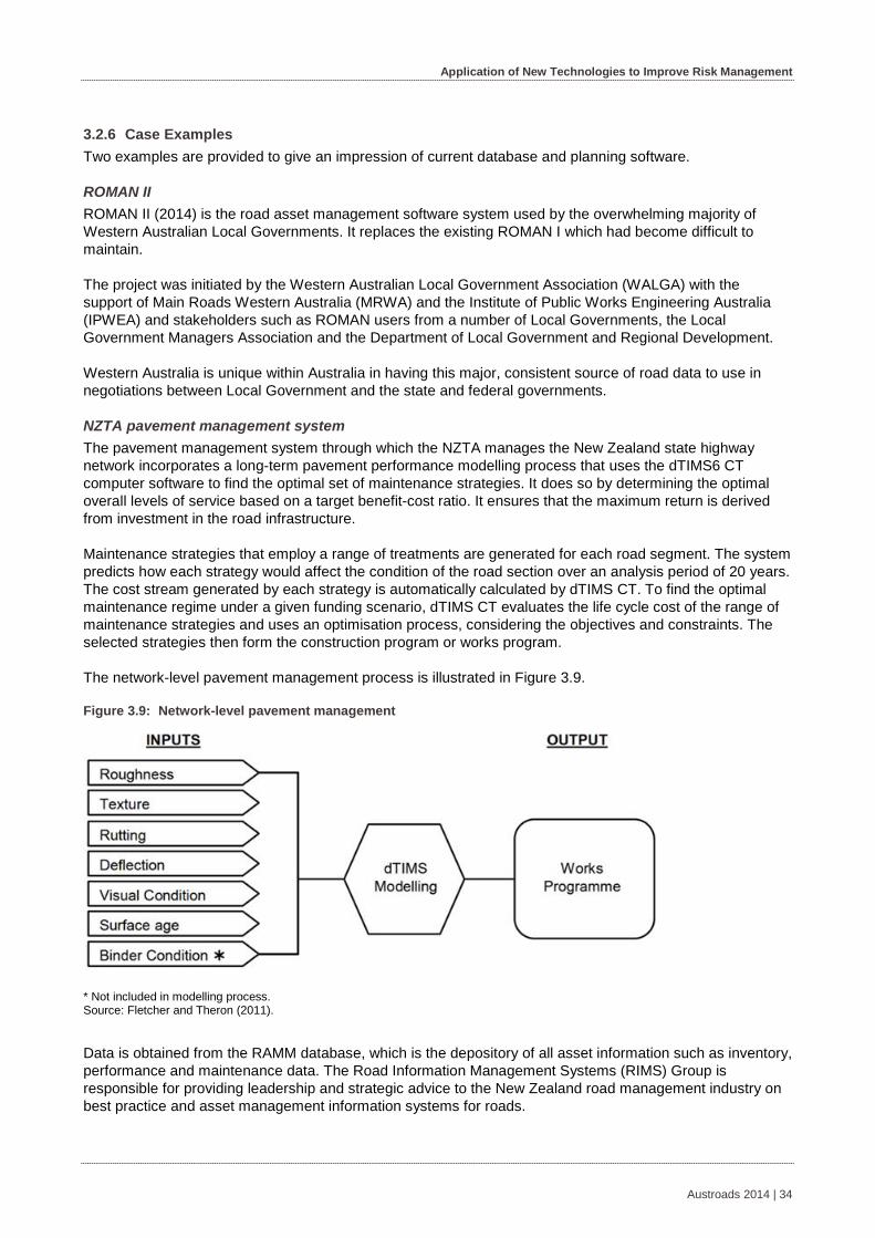
Application of New Technologies to Improve Risk Management
Case Examples 3.2.6Two examples are provided to give an impression of current database and planning software.
ROMAN II ROMAN II (2014) is the road asset management software system used by the overwhelming majority of Western Australian Local Governments. It replaces the existing ROMAN I which had become difficult to maintain.
The project was initiated by the Western Australian Local Government Association (WALGA) with the support of Main Roads Western Australia (MRWA) and the Institute of Public Works Engineering Australia (IPWEA) and stakeholders such as ROMAN users from a number of Local Governments, the Local Government Managers Association and the Department of Local Government and Regional Development.
Western Australia is unique within Australia in having this major, consistent source of road data to use in negotiations between Local Government and the state and federal governments.
NZTA pavement management system The pavement management system through which the NZTA manages the New Zealand state highway network incorporates a long-term pavement performance modelling process that uses the dTIMS6 CT computer software to find the optimal set of maintenance strategies. It does so by determining the optimal overall levels of service based on a target benefit-cost ratio. It ensures that the maximum return is derived from investment in the road infrastructure.
Maintenance strategies that employ a range of treatments are generated for each road segment. The system predicts how each strategy would affect the condition of the road section over an analysis period of 20 years. The cost stream generated by each strategy is automatically calculated by dTIMS CT. To find the optimal maintenance regime under a given funding scenario, dTIMS CT evaluates the life cycle cost of the range of maintenance strategies and uses an optimisation process, considering the objectives and constraints. The selected strategies then form the construction program or works program.
The network-level pavement management process is illustrated in Figure 3.9.
Figure 3.9: Network-level pavement management
* Not included in modelling process. Source: Fletcher and Theron (2011).
Data is obtained from the RAMM database, which is the depository of all asset information such as inventory, performance and maintenance data. The Road Information Management Systems (RIMS) Group is responsible for providing leadership and strategic advice to the New Zealand road management industry on best practice and asset management information systems for roads.
Austroads 2014 | 34

Application of New Technologies to Improve Risk Management
3.3 Wireless Sensor Network (WSN) for Condition Monitoring
Introduction 3.3.1‘Smart’ sensors with embedded microprocessors and wireless communication links have the potential to change fundamentally the way civil infrastructure systems such as Australia’s bridges, highways and buildings, are monitored, controlled, and maintained (Spencer et al. 2004).
Structural health monitoring (SHM) and control systems represent one of the primary applications of wireless sensor networks (WSN). SHM is a process that allows the estimation of the structural state and detection of structural change that affects the performance of a structure. This section will look into this primary application of wireless sensor networks.
A framework that can allow the distributed computing paradigm offered by smart sensors to be employed for SHM and control systems does not yet exist; current algorithms assume that all data is centrally collected and processed. Such an approach does not scale to systems with densely instrumented arrays of sensors that will be required for the next generation of SHM and control systems. However a framework that allows SHM assessment calculation based on wireless sensor data is currently under development (Illinois SHM project n.d.).
This section provides a brief introduction to WSN and identifies some of the opportunities and associated challenges.
Description of the Technology 3.3.2A WSN is a system of smart wirelessly connected sensors that allows for an automated procedure of gathering and processing data from traffic, raises structural health alarms and determines which traffic can be safely allowed on a bridge.
Wireless system architecture A WSN consists of sensor nodes attached to a structure to monitor physical or environmental conditions in real-time. Sensors communicate wirelessly to a data logger. A pilot study of the application of WSN for a steel bridge in NSW, monitored acceleration, strain and temperature at critical points (Boulis et al. 2011). The project is discussed in more detail in Section 3.3.7.
Figure 3.10 shows a WSN solution for SHM and Figure 3.11 shows the traditional wired system using a centralised architecture.
Austroads 2014 | 35
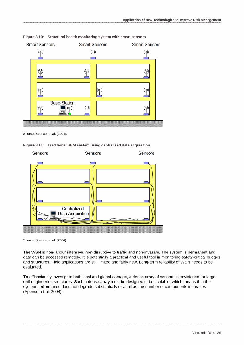
Application of New Technologies to Improve Risk Management
Figure 3.10: Structural health monitoring system with smart sensors
Source: Spencer et al. (2004).
Figure 3.11: Traditional SHM system using centralised data acquisition
Source: Spencer et al. (2004).
The WSN is non-labour intensive, non-disruptive to traffic and non-invasive. The system is permanent and data can be accessed remotely. It is potentially a practical and useful tool in monitoring safety-critical bridges and structures. Field applications are still limited and fairly new. Long-term reliability of WSN needs to be evaluated.
To efficaciously investigate both local and global damage, a dense array of sensors is envisioned for large civil engineering structures. Such a dense array must be designed to be scalable, which means that the system performance does not degrade substantially or at all as the number of components increases (Spencer et al. 2004).
Austroads 2014 | 36
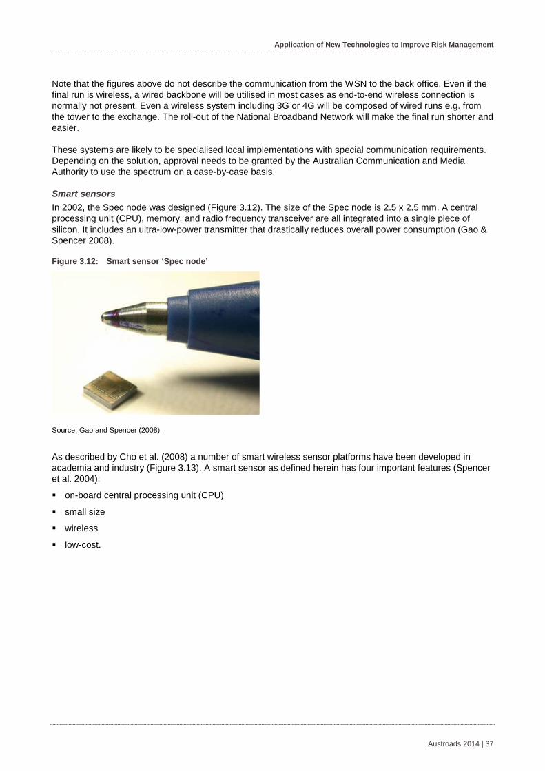
Application of New Technologies to Improve Risk Management
Note that the figures above do not describe the communication from the WSN to the back office. Even if the final run is wireless, a wired backbone will be utilised in most cases as end-to-end wireless connection is normally not present. Even a wireless system including 3G or 4G will be composed of wired runs e.g. from the tower to the exchange. The roll-out of the National Broadband Network will make the final run shorter and easier.
These systems are likely to be specialised local implementations with special communication requirements. Depending on the solution, approval needs to be granted by the Australian Communication and Media Authority to use the spectrum on a case-by-case basis.
Smart sensors In 2002, the Spec node was designed (Figure 3.12). The size of the Spec node is 2.5 x 2.5 mm. A central processing unit (CPU), memory, and radio frequency transceiver are all integrated into a single piece of silicon. It includes an ultra-low-power transmitter that drastically reduces overall power consumption (Gao & Spencer 2008).
Figure 3.12: Smart sensor ‘Spec node’
Source: Gao and Spencer (2008).
As described by Cho et al. (2008) a number of smart wireless sensor platforms have been developed in academia and industry (Figure 3.13). A smart sensor as defined herein has four important features (Spencer et al. 2004):
on-board central processing unit (CPU)
small size
wireless
low-cost.
Austroads 2014 | 37

Application of New Technologies to Improve Risk Management
Figure 3.13: Various smart wireless sensor platforms
Source: Cho et al. (2008).
Smart sensors can be used in an environment to both sense and actuate. Sensing requires that a physical or chemical phenomenon be converted to an electrical signal for display, processing, transmission, and/or recording. Actuation reverses this flow and converts an electrical signal to a physical or chemical change in the environment (Spencer et al. 2004).
Development status WSN are widely applied, however systems are still improving. Sensors are getting smaller, cheaper, longer lasting, and have more processing capabilities.
Applications matching the SHM standards are being developed. A new sensor board for one of the main off-the-shelf sensors, the Imote2, tailored to the requirements of SHM applications has been designed in 2008 (Rice et al. 2008). An open-source software library for SHM applications of Imote2, Illinois SHM Services Toolkit (http://shm.cs.uiuc.edu/software.html), has been developed with service oriented architecture to allow easy implementation of SHM algorithms on smart sensor networks (Nagayama et al. 2008 and Rice et al. 2008 in Cho et al. 2008).
Austroads 2014 | 38
Application of New Technologies to Improve Risk Management
Physical Principles 3.3.3
Wireless communication architecture Realising a smart sensor system requires the implementation of a decentralised approach composed of a modal identification algorithm and middleware services. Major numerical routines utilised in this approach include empirical modal decomposition, quick sort, and Hilbert transform. Middleware services for the SHM include data aggregation, reliable communication, and synchronised sensing. These functions are compatible with the smart sensors operating system. The time synchronisation and reliable data delivery mechanisms in the framework can be implemented respectively by using suitable existing techniques. The designs of distributed algorithms for WSN-based SHM are currently the subject of research. When the synchronised sensing is completed, the data acquired will be processed immediately. The measured acceleration time histories and the intermediate processed results, such as the structural modal parameters, are sent back to the back-end server, where damage alarm or other applications will be executed (Wu et al. 2013).
Smart sensors Generally, a smart wireless sensor is composed of three or four functional subsystems, being the sensing interface, the computational core, the wireless transceiver, and in some cases an actuation interface (Lynch & Loh 2006).
The sensing interface is an interface to which sensors can be connected and an analogue-to-digital converter.
The computational core generally consists of a microcontroller for the computational tasks, a random access memory to stack the measured and processed data, and a flash memory with software programs for the system operation and data processing.
The wireless transceiver is an integral component of the wireless system, which is composed of a radio frequency modem and antenna to communicate the processing information with other wireless sensors and to transfer the processed data to a remote data server (Cho et al. 2008).
Use and Limitations 3.3.4
Current practice Roads and Maritime Services (RMS) are responsible for maintaining the roads and bridges in New South Wales. RMS currently monitors the structural health of each bridge using the following procedure. Depending on bridge characteristics such as age, materials and design, as well as vehicle traffic, a bridge has a fixed schedule of on-site test visits. This is usually with a period of one year or more. In every on-site visit, a team of technicians instruments the bridge with strain gauges and/or displacement sensors. A series of controlled tests is undertaken where a known load is driven on the bridge, and the response of the sensors is stored on data-loggers.
A disadvantage of this procedure is that during these tests, the bridge is either closed down to traffic, or traffic is impeded by the slow passes of the heavy test truck.
Wireless sensor networks present opportunities for more automation, fewer human-hours of labour and less disruption of vehicle traffic (Boulis et al. 2011).
A traditional approach for wired sensing consists of conventional piezoelectric accelerometers hardwired to data acquisition boards residing in a personal computer. There are several drawbacks compared to WSN. The first drawback is that such a system includes the high cost of installation and disturbance of the normal operation of the structure due to wires having to run all over the structure. The second drawback is the high cost of the equipment. The third drawback is the cost of maintenance. (Kim et al. 2007).
Austroads 2014 | 39

Application of New Technologies to Improve Risk Management
In conventional SHM systems, the expensive cost for purchase and installation of system components, such as sensors, data loggers, computers, and connecting cables, is a big barrier to application. To guarantee that measurement data are reliably collected, SHM systems generally employ coaxial wires for communication between sensors and the repository. However, the installation of coaxial wires in structures is generally very expensive and labour-intensive. (Cho et al. 2008).
Possible uses WSN is used outside the road asset management domain as well, for instance for monitoring of mechanical machines, condition-based monitoring, volcano monitoring, earthquake monitoring, landslides and SHM. This report focusses on SHM applications to civil infrastructures to improve road asset management, and especially focusses on bridges.
SHM is a process that allows the estimation of the structural state and detection of structural change that affects the performance of a structure. Two discriminating factors in SHM are the time-scale of the change (how quickly the state changes) and the severity of the change. These factors represent two major sources of system change: alarm warnings (e.g. disaster notification for earthquake, explosion, etc.) and continuous health monitoring (e.g. from ambient vibrations, wind, etc.).
Spencer et al. (2004) identify some of the possible uses of WSN and state that the ability to continuously monitor the integrity of structures in real time can provide for increased safety to the public, particularly with regard to the aging structures in use today. By detecting damage at an early stage, WSN have the capability to mitigate structural dynamic response and prevent structures from reaching their limit states. This can reduce the costs and down-time associated with repair of critical damage. Observing, controlling, or even predicting the onset of dangerous structural behaviour, such as ‘flutter’ in bridges, can allow for repair or removal of the structure before lives are endangered.
In addition to controlling and monitoring long-term degradation, assessment of structural integrity after catastrophic events, such as earthquakes, floods or fires, is vital. This assessment can be a significant expense (both in time and money). After an earthquake, typically large numbers of buildings need to have their moment-resisting connections inspected. Additionally, structures internally, but not obviously, damaged in an earthquake may be in great danger of collapse during aftershocks; structural integrity assessment can help to identify such structures to enable evacuation of building occupants and contents prior to aftershocks. Furthermore, after natural disasters, it is important that emergency facilities and evacuation routes, including bridges and highways, be assessed for safety. The need for effective SHM is clear, with the primary goals of such systems being to enhance safety and reliability and to reduce maintenance and inspection costs.
Compared to the data collected periodically during a site visit as is currently common, an on-site test bed such as WSN can gather continuous health information over a long-term that will be used by e.g. structural engineering researchers.
Limitations Though the smart wireless sensor technology has been rapidly improving, there still remain limitations in hardware, software, and energy supply technology.
Hardware issues to be improved are wireless communication range, data transmission rate, and high-frequency sampling capability. It is expected however that hardware problems may be solved relatively fast due to rapid developments in electronics technology.
Software technology for the full utilisation of the hardware and for the complete assessment of structural health has been progressing slower than the hardware technology. It requires multidisciplinary collaboration among engineers in civil, mechanical, electrical, and computer science engineering.
The battery technology is improving slowest. Research efforts are focused on increasing the battery life, for example by optimising the WSN to reduce power consumption, improved wireless communication technology, and by energy harvesting (Cho et al. 2008).
Austroads 2014 | 40

Application of New Technologies to Improve Risk Management
Previous applications of WSN in SHM generally do not scale to a long enough multi-hop network needed to cover a large structure, and have not been implemented and tested in a harsh real-life environment (Engel et al. 2004, Lynch 2004, Spencer et al. 2004). However, in the case of the Golden Gate Bridge, Kim et al. (2007) demonstrated that this is possible. The Golden Gate Bridge case did provide a few implications for WSN, which can be interesting research topics. It was found that a small packet size is a bottleneck for network data transmission bandwidth, but increasing packet size is not a good solution due to the limited amount of available RAM (random access memory); a limitation resulting from an unshared buffer pool.
Another communication related limitation is the possible interference of the communication equipment with other systems, especially in urban or industrial areas. Bandwidth licensing is generally not an issue as most of the communication technologies are on free bandwidths (e.g. Bluetooth, WiFi, WiMax) or communication service providers (e.g. 3G).
While the opportunities offered by smart sensing for SHM are substantial, a number of critical issues need to be addressed before this potential can be realised. So, although WSN have been used for smaller structures extensively, due to these limitations, further technological improvements are still required for the smart wireless sensor technology in order to become an economical and reliable tool for SHM of large and complex structural systems (Cho et al. 2008).
When assessing the value of WSN against the three main questions in asset management (What do we own? What is the condition? What is the performance?), WSN is not able to answer which assets there are, is very well able to answer which conditions the assets are in, and is able to answer what the performance of the assets is.
Standards 3.3.5WSN has different components, being the smart sensors, the operating system and the wireless communication architecture. These components use different standards and protocols and are discussed below. Additional to the standards for the components, there are relevant standards for the system as a whole, like the SHM standards.
Off-the-shelf sensors There are a number of commercial off-the-shelf standards available. Alves (2009) has listed and categorised them by node type and typical application, as shown in Figure 3.14. Sensors used in SHM are for example the iMote1 and iMote2 sensors.
Figure 3.14: Smart sensor types
Source: Alves (2009).
Austroads 2014 | 41
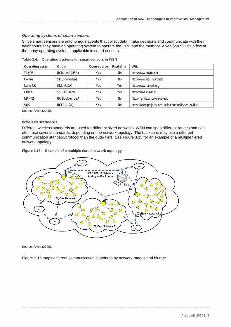
Application of New Technologies to Improve Risk Management
Operating systems of smart sensors Since smart sensors are autonomous agents that collect data, make decisions and communicate with their neighbours, they have an operating system to operate the CPU and the memory. Alves (2009) lists a few of the many operating systems applicable in smart sensors.
Table 3.4: Operating systems for smart sensors in WSN
Operating system Origin Open source Real-time URL
TinyOS UCB, Intel (USA) Yes No http://www.tinyos.net
Contiki SICS (Sweden) Yes No http://www.sics.se/contiki
Nano-RK CMU (USA) Yes Yes http://www.nanork.org
ERIKA SSSUP (Italy) Yes Yes http://erika.sssup.it
MANTIS UC Boulder (USA) Yes No http://mantis.cs.colorado.edu
SOS UCLA (USA) Yes No https://www.projects.nesi.ucla.edu/public/sos-2x/doc Source: Alves (2009).
Wireless standards Different wireless standards are used for different sized networks. WSN can span different ranges and can often use several standards, depending on the network topology. The backbone may use a different communication standard/protocol than the outer tiers. See Figure 3.15 for an example of a multiple tiered network topology.
Figure 3.15: Example of a multiple tiered network topology
Source: Alves (2009).
Figure 3.16 maps different communication standards by network ranges and bit rate.
Austroads 2014 | 42
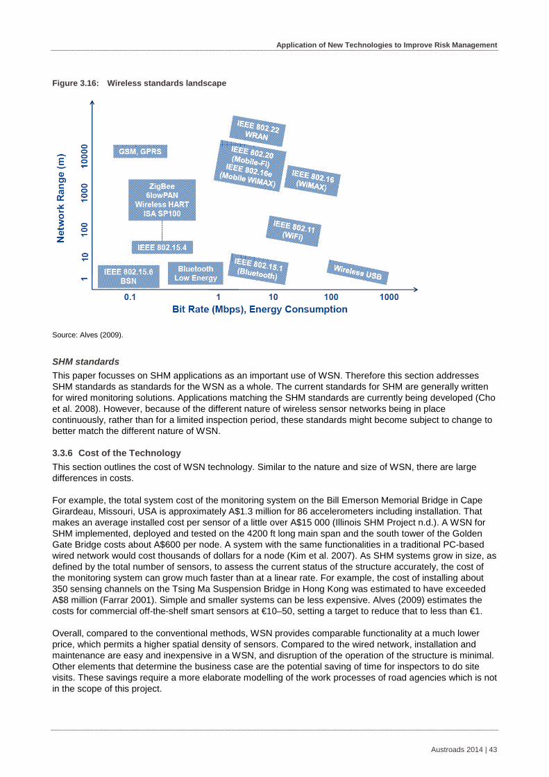
Application of New Technologies to Improve Risk Management
Figure 3.16: Wireless standards landscape
Source: Alves (2009).
SHM standards This paper focusses on SHM applications as an important use of WSN. Therefore this section addresses SHM standards as standards for the WSN as a whole. The current standards for SHM are generally written for wired monitoring solutions. Applications matching the SHM standards are currently being developed (Cho et al. 2008). However, because of the different nature of wireless sensor networks being in place continuously, rather than for a limited inspection period, these standards might become subject to change to better match the different nature of WSN.
Cost of the Technology 3.3.6This section outlines the cost of WSN technology. Similar to the nature and size of WSN, there are large differences in costs.
For example, the total system cost of the monitoring system on the Bill Emerson Memorial Bridge in Cape Girardeau, Missouri, USA is approximately A$1.3 million for 86 accelerometers including installation. That makes an average installed cost per sensor of a little over A$15 000 (Illinois SHM Project n.d.). A WSN for SHM implemented, deployed and tested on the 4200 ft long main span and the south tower of the Golden Gate Bridge costs about A$600 per node. A system with the same functionalities in a traditional PC-based wired network would cost thousands of dollars for a node (Kim et al. 2007). As SHM systems grow in size, as defined by the total number of sensors, to assess the current status of the structure accurately, the cost of the monitoring system can grow much faster than at a linear rate. For example, the cost of installing about 350 sensing channels on the Tsing Ma Suspension Bridge in Hong Kong was estimated to have exceeded A$8 million (Farrar 2001). Simple and smaller systems can be less expensive. Alves (2009) estimates the costs for commercial off-the-shelf smart sensors at €10–50, setting a target to reduce that to less than €1.
Overall, compared to the conventional methods, WSN provides comparable functionality at a much lower price, which permits a higher spatial density of sensors. Compared to the wired network, installation and maintenance are easy and inexpensive in a WSN, and disruption of the operation of the structure is minimal. Other elements that determine the business case are the potential saving of time for inspectors to do site visits. These savings require a more elaborate modelling of the work processes of road agencies which is not in the scope of this project.
Austroads 2014 | 43
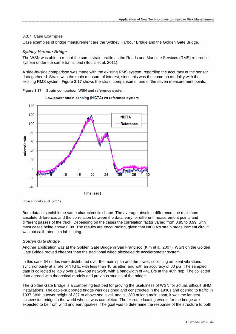
Application of New Technologies to Improve Risk Management
Case Examples 3.3.7Case examples of bridge measurement are the Sydney Harbour Bridge and the Golden Gate Bridge.
Sydney Harbour Bridge The WSN was able to record the same strain profile as the Roads and Maritime Services (RMS) reference system under the same traffic load (Boulis et al. 2011).
A side-by-side comparison was made with the existing RMS system, regarding the accuracy of the sensor data gathered. Strain was the main measure of interest, since this was the common modality with the existing RMS system. Figure 3.17 shows the strain comparison of one of the seven measurement points.
Figure 3.17: Strain comparison WSN and reference system
Source: Boulis et al. (2011).
Both datasets exhibit the same characteristic shape. The average absolute difference, the maximum absolute difference, and the correlation between the data, vary for different measurement points and different passes of the truck. Depending on the cases the correlation factor varied from 0.95 to 0.99, with most cases being above 0.98. The results are encouraging, given that NICTA’s strain measurement circuit was not calibrated in a lab setting.
Golden Gate Bridge Another application was at the Golden Gate Bridge in San Francisco (Kim et al. 2007). WSN on the Golden Gate Bridge proved cheaper than the traditional wired piezoelectric accelerometer system.
In this case 64 nodes were distributed over the main span and the tower, collecting ambient vibrations synchronously at a rate of 1 KHz, with less than 10 μs jitter, and with an accuracy of 30 μG. The sampled data is collected reliably over a 46–hop network, with a bandwidth of 441 B/s at the 46th hop. The collected data agreed with theoretical models and previous studies of the bridge.
The Golden Gate Bridge is a compelling test bed for proving the usefulness of WSN for actual, difficult SHM installations. The cable-supported bridge was designed and constructed in the 1930s and opened to traffic in 1937. With a tower height of 227 m above sea level, and a 1280 m long main span, it was the longest suspension bridge in the world when it was completed. The extreme loading events for the bridge are expected to be from wind and earthquakes. The goal was to determine the response of the structure to both
Austroads 2014 | 44

Application of New Technologies to Improve Risk Management
ambient and extreme conditions and compare actual behaviour to design predictions. The network measured ambient structural accelerations from wind load at closely spaced locations, as well as strong shaking from a possible earthquake, all at low cost and without interfering with the operation of the bridge. For this deployment, 64 sensors were deployed over the main span and southern tower, and were the largest WSN ever installed for SHM purposes by 2007 (Kim et al. 2007).
Austroads 2014 | 45

Application of New Technologies to Improve Risk Management
4. Level 2 Priority Technologies
4.1 Automatic Detection of Overweight Vehicles
Introduction 4.1.1Automatic detection of overweight vehicles uses a combination of weigh-in-motion (WIM) technology and automatic number plate recognition (ANPR) technology, the former to discreetly detect a vehicle and quantify its weight, and the latter to link that evaluation to a particular vehicle.
There are different reasons to assess the weight of vehicles, each with different requirements and different methods. Figure 4.1 shows an overview of the methods for mass monitoring. The scope of this section is limited to the specific combination of WIM technology and ANPR. This combination can be used to assist in the enforcement of weight restriction on a stretch of road or bridge and can help prevent pavement and structure deterioration and improve road safety.
Figure 4.1: Methods for mass monitoring
Source: Modified from Karl and Han (2007).
Weighing stations often exceed capacity at peak traffic times, and are forced to close while the back-log of trucks is cleared. When using WIM and ANPR, the weighing station can be used for high risk vehicles, allowing weight compliant carriers with good safety records to bypass the weigh station. The use and limitations of WIM and ANPR are described in more detail in Section 4.1.4.
Description of the Technology 4.1.2Automatic detection of overweight vehicles is a combination of WIM and ANPR. Both technologies are described, as well as some issues that have been experienced with the integration of the two systems.
Weigh-in-motion A WIM system is a device which measures the dynamic axle weight of a moving vehicle to estimate the corresponding static axle weight (Koniditsiotis et al. 1995).
The weigh-in-motion market remains especially buoyant and technological development continues to reflect this. Both the numbers of countries using WIM technology and the numbers of systems that they deploy are on the increase. WIM is often combined with other technologies to realise or extend applications (ITS International 2009).
Austroads 2014 | 46
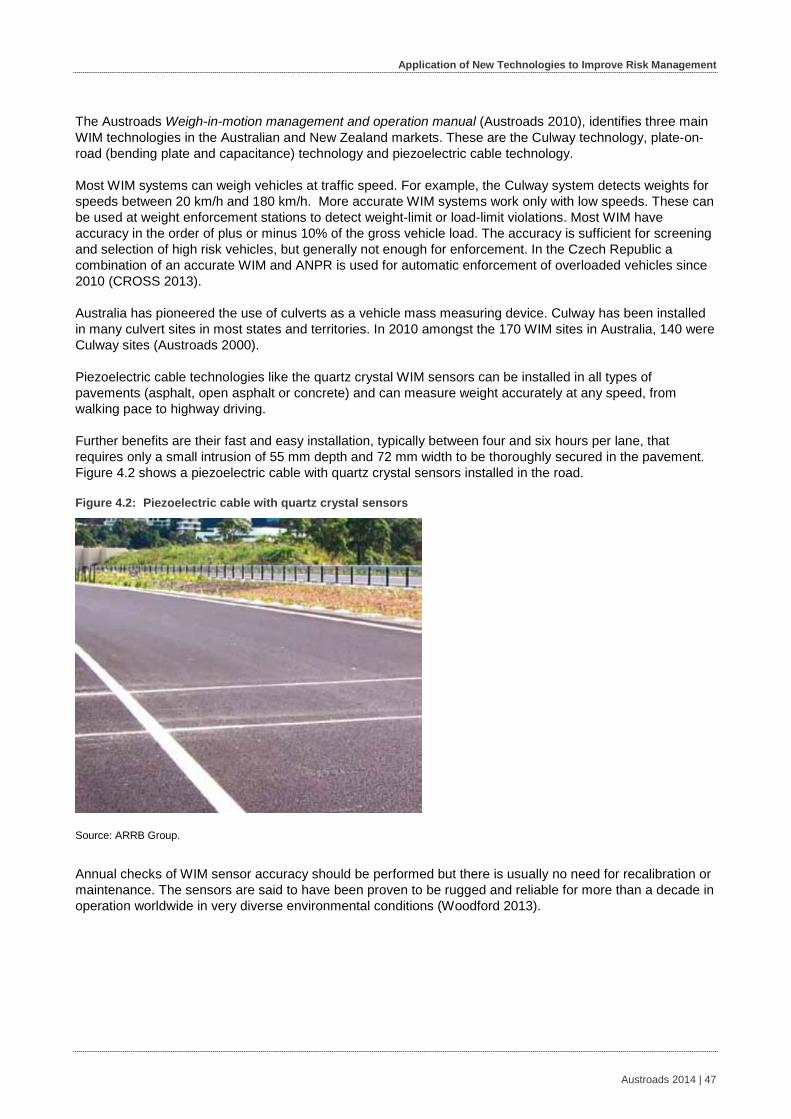
Application of New Technologies to Improve Risk Management
The Austroads Weigh-in-motion management and operation manual (Austroads 2010), identifies three main WIM technologies in the Australian and New Zealand markets. These are the Culway technology, plate-on-road (bending plate and capacitance) technology and piezoelectric cable technology.
Most WIM systems can weigh vehicles at traffic speed. For example, the Culway system detects weights for speeds between 20 km/h and 180 km/h. More accurate WIM systems work only with low speeds. These can be used at weight enforcement stations to detect weight-limit or load-limit violations. Most WIM have accuracy in the order of plus or minus 10% of the gross vehicle load. The accuracy is sufficient for screening and selection of high risk vehicles, but generally not enough for enforcement. In the Czech Republic a combination of an accurate WIM and ANPR is used for automatic enforcement of overloaded vehicles since 2010 (CROSS 2013).
Australia has pioneered the use of culverts as a vehicle mass measuring device. Culway has been installed in many culvert sites in most states and territories. In 2010 amongst the 170 WIM sites in Australia, 140 were Culway sites (Austroads 2000).
Piezoelectric cable technologies like the quartz crystal WIM sensors can be installed in all types of pavements (asphalt, open asphalt or concrete) and can measure weight accurately at any speed, from walking pace to highway driving.
Further benefits are their fast and easy installation, typically between four and six hours per lane, that requires only a small intrusion of 55 mm depth and 72 mm width to be thoroughly secured in the pavement. Figure 4.2 shows a piezoelectric cable with quartz crystal sensors installed in the road.
Figure 4.2: Piezoelectric cable with quartz crystal sensors
Source: ARRB Group.
Annual checks of WIM sensor accuracy should be performed but there is usually no need for recalibration or maintenance. The sensors are said to have been proven to be rugged and reliable for more than a decade in operation worldwide in very diverse environmental conditions (Woodford 2013).
Austroads 2014 | 47

Application of New Technologies to Improve Risk Management
Automatic number plate recognition Automatic number plate recognition is a technology that automatically reads vehicle registration plates and compares these details against database systems. An image of a number plate or number plate patch is saved and checked against local and national databases, providing feedback to the operators in seconds (UK National Policing Improvement Agency 2009).
The capability of the reader dictates the number of vehicles that can be read. Each camera has a capacity to read up to 3600 number plates per hour. Cameras can be static, CCTV-integrated or mobile. Cameras are also available with infrared capability, allowing them to operate over a 24-hour period in low-light situations.
ANPR data comprises ‘read’ data and ‘hit’ data. Read data is the data collected as vehicles pass through the ANPR reader. A hit is a match to a record of a vehicle in the database. Additional data include:
a digitalised picture
the time and date the data was captured
the location and other details of the camera.
System integration issues For a complex vehicle, a combination of traditional inductive loops and WIM sensors is used to first detect each individual axle group and its timing, and then weigh it. Knowledge of this information on each vehicle wheel makes it possible to calculate the loads per axle group, the total vehicle weight, and from this, determine the category and speed of the vehicle. This information and an image of the vehicle and its number plate can be recorded by ANPR technology in cases of exceeding the weight or speed limits, and stored in a database or made available immediately for enforcement (Woodford 2013).
The WIM system has to be able to process the signals from in-road sensors and produce a time-stamped vehicle record. Different vehicle lengths, axle configurations and speeds mean processing times are not uniform. Clock drift in the pairing server and in the WIM system needs to be taken into account (ITS International 2009).
Physical Principles 4.1.3
Weigh-in-motion – culvert This system weighs and classifies traffic by using mechanical strain gauges deployed in a box culvert (Figure 4.3). It uses a flexible insulating material, typically a copper wire, adhered to a rigid material. As a vehicle axle passes over the structure or housing, the induced strain is measured and related to the mass. The system employs two piezoelectric sensors, placed 10 m apart in each instrumented culvert.
Figure 4.3: A Culway site and Culway II data logger
Source: ARRB Group.
Austroads 2014 | 48

Application of New Technologies to Improve Risk Management
Weigh-in-motion – plate-on-road technology There are two types of plate-on-road technologies, being the bending plate technology and the capacitance pad.
The bending plate technology incorporates steel plates, with strain gauges permanently attached to their underside such that the strain gauges behave as one with the plates. The strain gauges develop a strain signal proportional to the deflection of the plate under a vehicle axle. The strain signal is amplified and processed to produce the vehicle axle mass.
The capacitance pad mass sensor is a rubber and steel mat device. The pad comprises three sheets of steel separated by a soft rubber dielectric material. Compression of the pad under a vehicle axle produces an increase in capacitance, which is interpreted as a mass.
Weigh-in-motion – piezoelectric cable with quartz crystal sensors The piezoelectric cable is usually mounted in an aluminium U-shaped channel. The channel is placed into the road surface (Figure 4.4). The passage of a vehicle axle over the cable creates a wave form of current that is proportional to the axle mass.
Figure 4.4: Quartz weigh-in-motion site profile
Source: Woodford (2013).
Automatic number plate recognition An automatic number plate recognition system uses optical character recognition (OCR) software to scan each group of pixels and estimate whether or not it could be a letter and replaces the pixels with the ASCII code for the letter.
Different systems have different ways to collect the images. Some systems only take one image at a certain position. Others take a series of snapshots as a vehicle approaches the camera. The list of snapshots is scanned for similarities and a favourite selected to retain.
Most ANPR systems use infrared cameras and infrared illuminators to light the number plates. This means the cameras do not need to change their setting due to the huge variety of lighting conditions, e.g. day-time, night-time, sunlight, backlight, headlights in the visible spectrum. Number plates in most countries are retro-reflective. The surface of the number plate is made to reflect the light back to the source. No matter from which direction the light is directed, it always reflects back and makes them very visible. The infrared illumination from the illuminator will be reflected directly back to the camera. The picture will be mostly black with no detail except for the number plate. The OCR software then takes care of converting the image to usable code (Constant n.d.).
Austroads 2014 | 49
Application of New Technologies to Improve Risk Management
Use and Limitations 4.1.4As opposed to, for example, on-board mass monitoring technologies, where the mass of equipped vehicles can be monitored throughout their journey, WIM and ANPR measure only at a specific location, but do measure all passing vehicles. The combination of WIM and ANPR is used at specific locations to protect bridges and sections of highways from damage caused by overweight vehicles and to improve road safety. It is generally used for real-time pre-selection of overweight vehicles for enforcement. A second common application is 'tolling-by-weight'. Both uses and their limitations are described.
Pre-selection for enforcement The combination of WIM and ANPR cameras is especially useful for pre-selection for enforcement.
Enforcement of weight limits on bridges and roads will allow asset managers to better protect their assets from accelerated deterioration due to overloaded vehicles.
Because the accuracy of traffic speed WIM systems is generally too limited for direct enforcement, ANPR and WIM is used to pre-select overweight vehicles. For enforcement the American Society for Testing Materials guidelines suggest type IV low-speed WIM that can be used at weight enforcement stations to detect weight-limit or load-limit violations at speeds from 3 to 16 km/h. The accuracies are shown in Table 4.1.
The details of the overweight vehicles are sent to the police who can pull over the overweight vehicles for an official weight measurement at a weighing station.
WIM systems that are not linked to an ANPR system have other applications as well. Koniditsiotis et al. (1995) identified a number of Australian uses and applications of WIM, which can be categorised into three main areas as follow:
infrastructure design and management
freight/trade planning and regulation
enforcement and detection.
Tolling-by-weight Toll fees are usually based on the distance travelled and the class of vehicle. However, this type of tolling does not take into account if the vehicle is loaded or not. It is the overloading which increases maintenance costs due to additional highway surface damage. WIM systems are capable of measuring the actual axle loads and vehicle weight of each vehicle passing a road section. The addition of WIM to an existing tolling system offers a tolling-by-weight capability. In cases of overloading, an additional penalty fee can be applied.
In China, WIM systems are used to calculate toll fees based on the vehicle weight. WIM sensors have been installed in hundreds of the country's toll lanes since 2007, around 22 m before the toll booths. Many of these installations have taken place within the last six months (Woodford 2013).
WIM sensors can be installed at toll booths under low speed or stop and go conditions, or at a toll gantry under free-flow high speed conditions.
WIM technology has been used in a number of significant highway tolling projects across the world, including 20 high speed systems for overweight pre-selection and enforcement in Saudi Arabia (Woodford 2013).
Austroads 2014 | 50
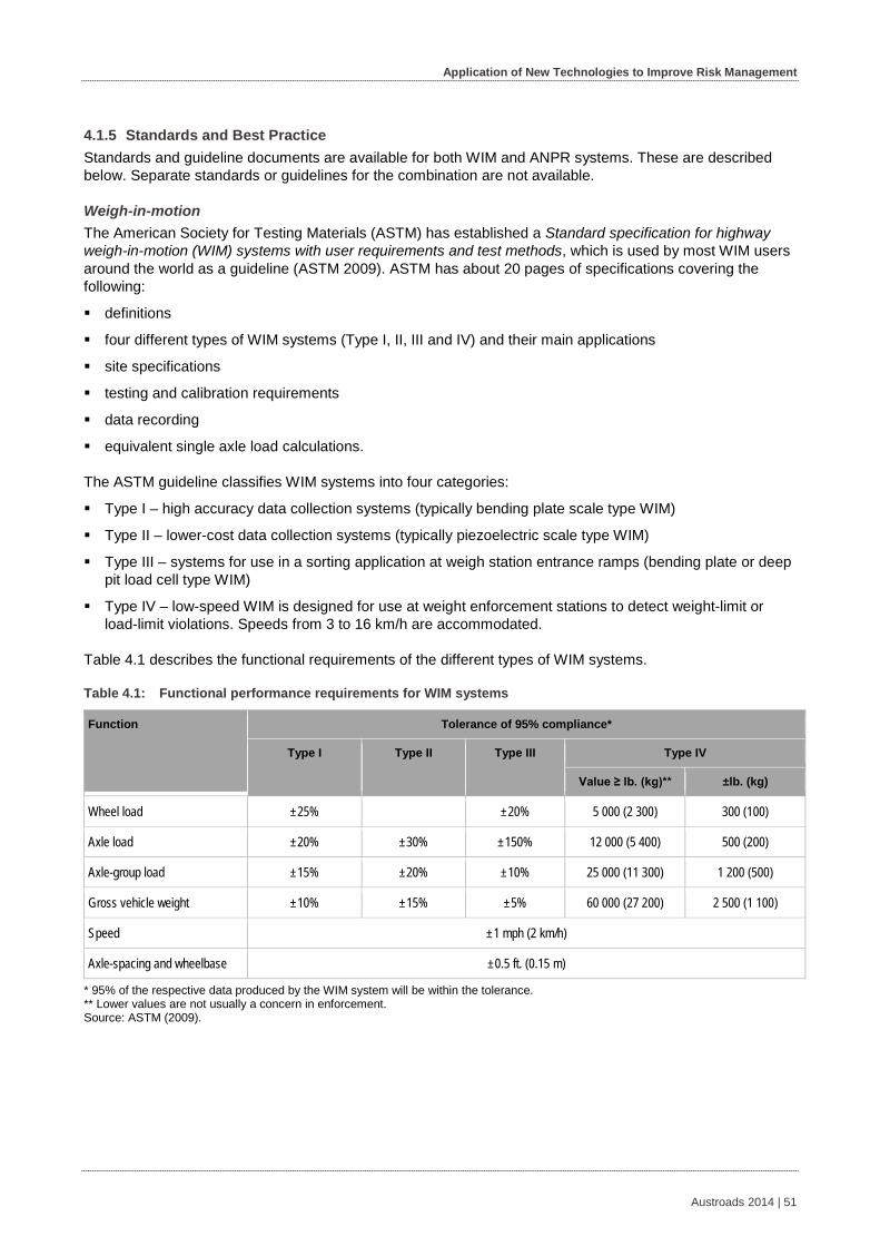
Application of New Technologies to Improve Risk Management
Standards and Best Practice 4.1.5Standards and guideline documents are available for both WIM and ANPR systems. These are described below. Separate standards or guidelines for the combination are not available.
Weigh-in-motion The American Society for Testing Materials (ASTM) has established a Standard specification for highway weigh-in-motion (WIM) systems with user requirements and test methods, which is used by most WIM users around the world as a guideline (ASTM 2009). ASTM has about 20 pages of specifications covering the following:
definitions
four different types of WIM systems (Type I, II, III and IV) and their main applications
site specifications
testing and calibration requirements
data recording
equivalent single axle load calculations.
The ASTM guideline classifies WIM systems into four categories:
Type I – high accuracy data collection systems (typically bending plate scale type WIM)
Type II – lower-cost data collection systems (typically piezoelectric scale type WIM)
Type III – systems for use in a sorting application at weigh station entrance ramps (bending plate or deep pit load cell type WIM)
Type IV – low-speed WIM is designed for use at weight enforcement stations to detect weight-limit or load-limit violations. Speeds from 3 to 16 km/h are accommodated.
Table 4.1 describes the functional requirements of the different types of WIM systems.
Table 4.1: Functional performance requirements for WIM systems
Function Tolerance of 95% compliance*
Type I Type II Type III Type IV
Value ≥ lb. (kg)** ±lb. (kg)
Wheel load ±25% ±20% 5 000 (2 300) 300 (100)
Axle load ±20% ±30% ±150% 12 000 (5 400) 500 (200)
Axle-group load ±15% ±20% ±10% 25 000 (11 300) 1 200 (500)
Gross vehicle weight ±10% ±15% ±5% 60 000 (27 200) 2 500 (1 100)
Speed ±1 mph (2 km/h)
Axle-spacing and wheelbase ±0.5 ft. (0.15 m)
* 95% of the respective data produced by the WIM system will be within the tolerance. ** Lower values are not usually a concern in enforcement. Source: ASTM (2009).
Austroads 2014 | 51
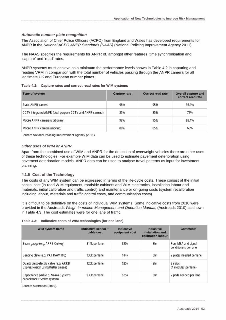
Application of New Technologies to Improve Risk Management
Automatic number plate recognition The Association of Chief Police Officers (ACPO) from England and Wales has developed requirements for ANPR in the National ACPO ANPR Standards (NAAS) (National Policing Improvement Agency 2011).
The NAAS specifies the requirements for ANPR of, amongst other features, time synchronisation and ‘capture’ and ‘read’ rates.
ANPR systems must achieve as a minimum the performance levels shown in Table 4.2 in capturing and reading VRM in comparison with the total number of vehicles passing through the ANPR camera for all legitimate UK and European number plates.
Table 4.2: Capture rates and correct read rates for WIM systems
Type of system Capture rate Correct read rate Overall capture and correct read rate
Static ANPR camera 98% 95% 93.1%
CCTV integrated ANPR (dual purpose CCTV and ANPR camera) 85% 85% 72%
Mobile ANPR camera (stationary) 98% 95% 93.1%
Mobile ANPR camera (moving) 80% 85% 68%
Source: National Policing Improvement Agency (2011).
Other uses of WIM or ANPR Apart from the combined use of WIM and ANPR for the detection of overweight vehicles there are other uses of these technologies. For example WIM data can be used to estimate pavement deterioration using pavement deterioration models. ANPR data can be used to analyse travel patterns as input for investment planning.
Cost of the Technology 4.1.6The costs of any WIM system can be expressed in terms of the life-cycle costs. These consist of the initial capital cost (in-road WIM equipment, roadside cabinets and WIM electronics, installation labour and materials, initial calibration and traffic control) and maintenance or on-going costs (system recalibration including labour, materials and traffic control costs, and communication costs).
It is difficult to be definitive on the costs of individual WIM systems. Some indicative costs from 2010 were provided in the Austroads Weigh-in-motion Management and Operation Manual, (Austroads 2010) as shown in Table 4.3. The cost estimates were for one lane of traffic.
Table 4.3: Indicative costs of WIM technologies (for one lane)
WIM system name Indicative sensor + cable cost
Indicative equipment cost
Indicative installation and
calibration labour
Comments
Strain gauge (e.g. ARRB Culway) $14k per lane $20k 8hr Four MSA and signal conditioners per lane
Bending plate (e.g. PAT DAW 100) $30k per lane $14k 6hr 2 plates needed per lane
Quartz piezoelectric cable (e.g. ARRB Express-weigh using Kistler Lineas)
$20k per lane $25k 2hr 2 strips (4 modules per lane)
Capacitance pad (e.g. Mikros Systems capacitance HSWIM system)
$30k per lane $25k 6hr 2 pads needed per lane
Source: Austroads (2010).
Austroads 2014 | 52
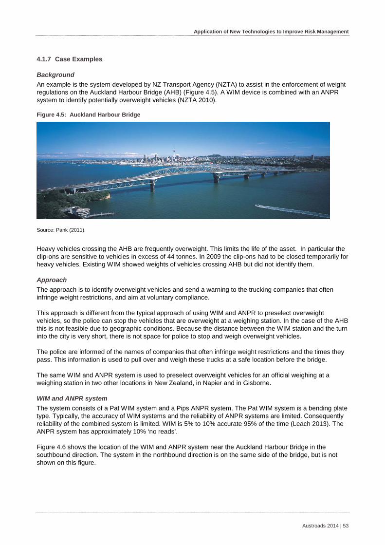
Application of New Technologies to Improve Risk Management
Case Examples 4.1.7
Background An example is the system developed by NZ Transport Agency (NZTA) to assist in the enforcement of weight regulations on the Auckland Harbour Bridge (AHB) (Figure 4.5). A WIM device is combined with an ANPR system to identify potentially overweight vehicles (NZTA 2010).
Figure 4.5: Auckland Harbour Bridge
Source: Pank (2011).
Heavy vehicles crossing the AHB are frequently overweight. This limits the life of the asset. In particular the clip-ons are sensitive to vehicles in excess of 44 tonnes. In 2009 the clip-ons had to be closed temporarily for heavy vehicles. Existing WIM showed weights of vehicles crossing AHB but did not identify them.
Approach The approach is to identify overweight vehicles and send a warning to the trucking companies that often infringe weight restrictions, and aim at voluntary compliance.
This approach is different from the typical approach of using WIM and ANPR to preselect overweight vehicles, so the police can stop the vehicles that are overweight at a weighing station. In the case of the AHB this is not feasible due to geographic conditions. Because the distance between the WIM station and the turn into the city is very short, there is not space for police to stop and weigh overweight vehicles.
The police are informed of the names of companies that often infringe weight restrictions and the times they pass. This information is used to pull over and weigh these trucks at a safe location before the bridge.
The same WIM and ANPR system is used to preselect overweight vehicles for an official weighing at a weighing station in two other locations in New Zealand, in Napier and in Gisborne.
WIM and ANPR system The system consists of a Pat WIM system and a Pips ANPR system. The Pat WIM system is a bending plate type. Typically, the accuracy of WIM systems and the reliability of ANPR systems are limited. Consequently reliability of the combined system is limited. WIM is 5% to 10% accurate 95% of the time (Leach 2013). The ANPR system has approximately 10% ‘no reads’.
Figure 4.6 shows the location of the WIM and ANPR system near the Auckland Harbour Bridge in the southbound direction. The system in the northbound direction is on the same side of the bridge, but is not shown on this figure.
Austroads 2014 | 53
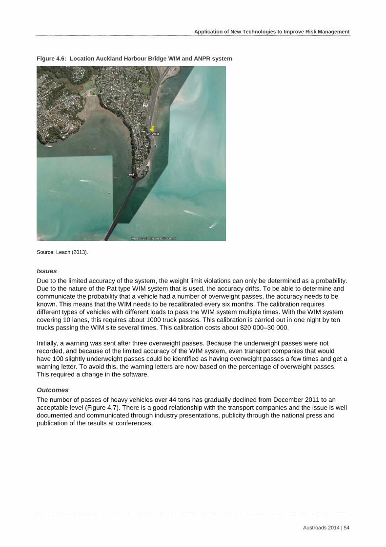
Application of New Technologies to Improve Risk Management
Figure 4.6: Location Auckland Harbour Bridge WIM and ANPR system
Source: Leach (2013).
Issues Due to the limited accuracy of the system, the weight limit violations can only be determined as a probability. Due to the nature of the Pat type WIM system that is used, the accuracy drifts. To be able to determine and communicate the probability that a vehicle had a number of overweight passes, the accuracy needs to be known. This means that the WIM needs to be recalibrated every six months. The calibration requires different types of vehicles with different loads to pass the WIM system multiple times. With the WIM system covering 10 lanes, this requires about 1000 truck passes. This calibration is carried out in one night by ten trucks passing the WIM site several times. This calibration costs about $20 000–30 000.
Initially, a warning was sent after three overweight passes. Because the underweight passes were not recorded, and because of the limited accuracy of the WIM system, even transport companies that would have 100 slightly underweight passes could be identified as having overweight passes a few times and get a warning letter. To avoid this, the warning letters are now based on the percentage of overweight passes. This required a change in the software.
Outcomes The number of passes of heavy vehicles over 44 tons has gradually declined from December 2011 to an acceptable level (Figure 4.7). There is a good relationship with the transport companies and the issue is well documented and communicated through industry presentations, publicity through the national press and publication of the results at conferences.
Austroads 2014 | 54

Application of New Technologies to Improve Risk Management
Figure 4.7: Number of overweight Auckland Harbour Bridge passes
Source: Leach (2013).
Figure 4.7 shows the decline in the number of Auckland Harbour Bridge passes of heavy vehicles over 44 tons. The orange lines indicate the period in which the first batch of warning letters was sent to transport companies.
4.2 On-board Mass Monitoring
Introduction 4.2.1As opposed to weigh-in-motion technology, on-board mass monitoring (OBM) is the measuring of a vehicle’s mass using on-board instrumentation. For trucks, this is achieved through sensors which measure the mass over each axle. These sensors can either be load cells, which measure mass based on the load applied to a strain gauge within the load cell, or air pressure transducers, which measure mass based on the air pressure within an axle’s airbag suspension.
Tare mass is the mass of a vehicle and its trailers when empty. Payload is the mass of the freight carried while gross mass is the combined mass of the vehicle, trailers and freight. Hence:
Gross mass = tare mass + payload mass
On-board mass monitoring allows the payload to be measured at the point of loading, permitting the driver to more accurately load the vehicle to legal weights over each axle group and redistribute or off-load the freight if needs be to achieve the legal weights. This eliminates the potential for lost revenue due to under loading or fines due to overloading. An overloaded vehicle will also experience undue wear and tear, slower travel times and will be a greater safety hazard on the road. Thus the commercial investment in OBM is justified through improvements in productivity and safety.
Austroads 2014 | 55

Application of New Technologies to Improve Risk Management
It is important to note that OBM only measures the masses above the sensors; it does not measure the mass of the axle or the tare mass. During calibration, the mass of the empty trailers is set to zero such that all mass readings are measures of just the payload mass. Typically, the tare mass is set at a certified weighbridge when the vehicle is empty. This tare mass is then added to the payload to arrive at the total mass.
Figure 4.8 details the main methods for mass monitoring. On-board mass monitoring is shown as the centre box.
Figure 4.8: Methods for mass monitoring
Source: Karl and Han (2007).
Potential applications of OBM for asset management are:
using OBM mass limits as a means of regulating heavy vehicle road access to limit their impact on road wear, bridges and traffic
using mass as measured by OBM as a factor in heavy vehicle road pricing
use of OBM dynamic data to identify and locate road deterioration
limit road wear due to poor vehicle suspension evident through spikes in OBM readings
calibration of on-road WIM systems.
These potential applications are described in Section 4.2.4.
Description of the Technology 4.2.2This section describes the various technologies and methods for OBM.
The essential component for mass monitoring is the mass sensor. Two principal types of sensors are used by the industry; load cells with strain gauges and air pressure transducers.
Load cells are typically used for mechanical suspensions as well as the turntable (fifth wheel) while air pressure transducers base their measurement upon the air pressures in the airbag suspension systems.
The fitment of an OBM system can be undertaken at the time the trailer is being constructed with additional after-market fitment of sensors and indicators to the prime mover or a complete fitment can be accomplished as an after-market sale.
Austroads 2014 | 56
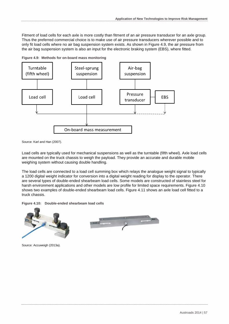
Application of New Technologies to Improve Risk Management
Fitment of load cells for each axle is more costly than fitment of an air pressure transducer for an axle group. Thus the preferred commercial choice is to make use of air pressure transducers wherever possible and to only fit load cells where no air bag suspension system exists. As shown in Figure 4.9, the air pressure from the air bag suspension system is also an input for the electronic braking system (EBS), where fitted.
Figure 4.9: Methods for on-board mass monitoring
Source: Karl and Han (2007).
Load cells are typically used for mechanical suspensions as well as the turntable (fifth wheel). Axle load cells are mounted on the truck chassis to weigh the payload. They provide an accurate and durable mobile weighing system without causing double handling.
The load cells are connected to a load cell summing box which relays the analogue weight signal to typically a 1200 digital weight indicator for conversion into a digital weight reading for display to the operator. There are several types of double-ended shearbeam load cells. Some models are constructed of stainless steel for harsh environment applications and other models are low profile for limited space requirements. Figure 4.10 shows two examples of double-ended shearbeam load cells. Figure 4.11 shows an axle load cell fitted to a truck chassis.
Figure 4.10: Double-ended shearbeam load cells
Source: Accuweigh (2013a).
Austroads 2014 | 57

Application of New Technologies to Improve Risk Management
Figure 4.11: Axle load cell fitted to a truck chassis
Source: Accuweigh (2013a).
Fifth wheel (turntable) load cells are used to measure the weight above the tractor unit’s rear axles when towing a trailer. They are more accurate than using load cells or air pressure transducers on the tractor’s rear axles, because the fifth wheel load cells eliminate the potential for inaccuracy caused by friction in the drive axle group suspension.
Fifth wheel load cells are designed to fit under Holland or Fontaine fifth wheel plates, replacing the standard risers or slide brackets. These load cells provide immediate weight information without adding substantially to the trailer height or the tractor weight.
Like axle load cells, they consist of double shear beams made from high strength alloy steel. The internal electronics are completely sealed and they are designed to bolt-on for easy installation and maintenance. Figure 4.12 shows fifth wheel load cells on a slider bracket.
Figure 4.12: Fifth wheel load cells on slider bracket
Source: Sparta (2009).
Air pressure transducers Air pressure transducers (APT) are connected to the air line of an airbag suspension system. Capacitive sensors are used to convert the gauge pressure detected in the airbags to a determination of the applied mass in kilograms. This is achieved through a diaphragm and pressure cavity to create a variable capacitor to detect strain due to applied pressure. Common technologies use metal, ceramic, and silicon diaphragms.
Austroads 2014 | 58
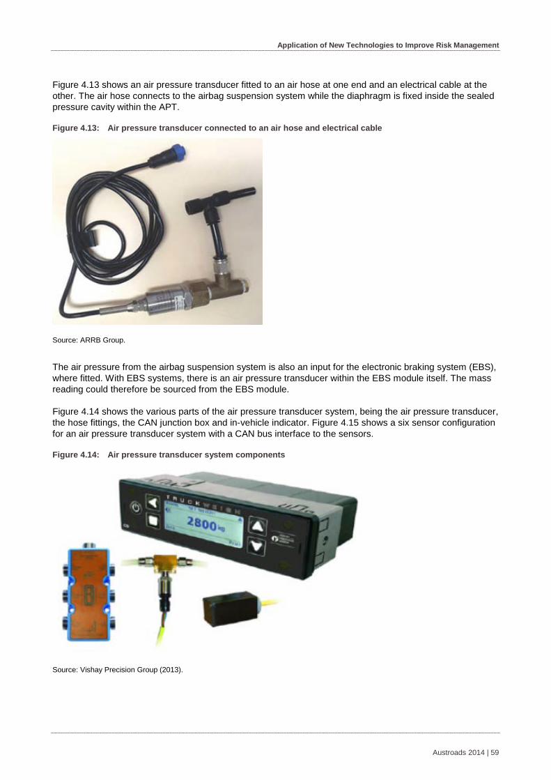
Application of New Technologies to Improve Risk Management
Figure 4.13 shows an air pressure transducer fitted to an air hose at one end and an electrical cable at the other. The air hose connects to the airbag suspension system while the diaphragm is fixed inside the sealed pressure cavity within the APT.
Figure 4.13: Air pressure transducer connected to an air hose and electrical cable
Source: ARRB Group.
The air pressure from the airbag suspension system is also an input for the electronic braking system (EBS), where fitted. With EBS systems, there is an air pressure transducer within the EBS module itself. The mass reading could therefore be sourced from the EBS module.
Figure 4.14 shows the various parts of the air pressure transducer system, being the air pressure transducer, the hose fittings, the CAN junction box and in-vehicle indicator. Figure 4.15 shows a six sensor configuration for an air pressure transducer system with a CAN bus interface to the sensors.
Figure 4.14: Air pressure transducer system components
Source: Vishay Precision Group (2013).
Austroads 2014 | 59

Application of New Technologies to Improve Risk Management
Figure 4.15: Six sensor air pressure transducer system
Source: Vishay Precision Group (2013).
The arrangement of the axle in conjunction with the airbag suspension and brakes can be seen in Figure 4.16.
Figure 4.16: Air suspension componentry using square axle beams
Source: BPW (2013).
Bluetooth weight indicators Bluetooth weight indicators enable wireless short-range communications while maintaining high levels of security. Low-power, they are ideal for transmitting weight, time and date data from a truck fitted with an on-board weighing system to a local yard office or weighbridge office. This eliminates the need for the driver to exit the truck to process a transaction, increasing efficiency in time and productivity. It is also safer for drivers in congested work areas.
Bluetooth radio waves do not need line of sight and many Bluetooth devices can send and receive information simultaneously and communicate with each other automatically. The most common type of Bluetooth works for a distance of around 10 metres. It sends out a relatively weak signal which helps avoid interference with other devices. A typical Bluetooth indicator is shown in Figure 4.17.
Austroads 2014 | 60
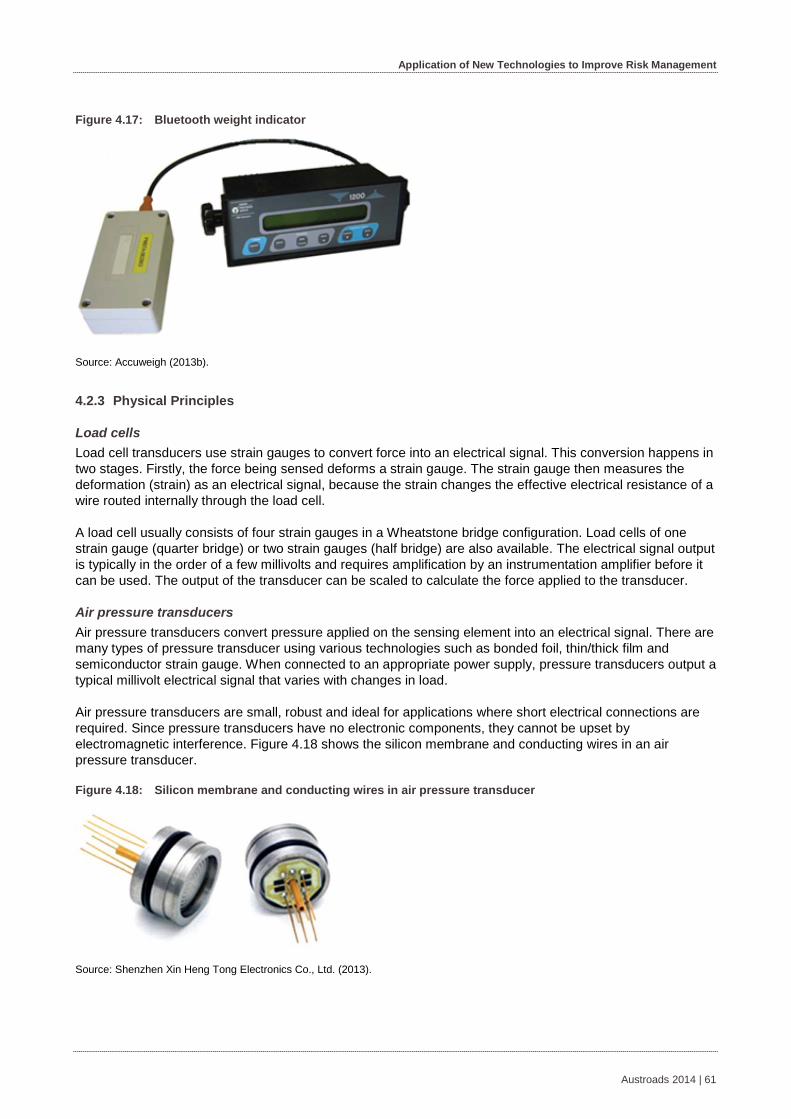
Application of New Technologies to Improve Risk Management
Figure 4.17: Bluetooth weight indicator
Source: Accuweigh (2013b).
Physical Principles 4.2.3
Load cells Load cell transducers use strain gauges to convert force into an electrical signal. This conversion happens in two stages. Firstly, the force being sensed deforms a strain gauge. The strain gauge then measures the deformation (strain) as an electrical signal, because the strain changes the effective electrical resistance of a wire routed internally through the load cell.
A load cell usually consists of four strain gauges in a Wheatstone bridge configuration. Load cells of one strain gauge (quarter bridge) or two strain gauges (half bridge) are also available. The electrical signal output is typically in the order of a few millivolts and requires amplification by an instrumentation amplifier before it can be used. The output of the transducer can be scaled to calculate the force applied to the transducer.
Air pressure transducers Air pressure transducers convert pressure applied on the sensing element into an electrical signal. There are many types of pressure transducer using various technologies such as bonded foil, thin/thick film and semiconductor strain gauge. When connected to an appropriate power supply, pressure transducers output a typical millivolt electrical signal that varies with changes in load.
Air pressure transducers are small, robust and ideal for applications where short electrical connections are required. Since pressure transducers have no electronic components, they cannot be upset by electromagnetic interference. Figure 4.18 shows the silicon membrane and conducting wires in an air pressure transducer.
Figure 4.18: Silicon membrane and conducting wires in air pressure transducer
Source: Shenzhen Xin Heng Tong Electronics Co., Ltd. (2013).
Austroads 2014 | 61

Application of New Technologies to Improve Risk Management
Use and Limitations 4.2.4
Possible asset management applications The following are some possible applications of OBM which could potentially improve on current best practices in road asset management.
Use of OBM as a determinant for heavy vehicle road access The Intelligent Access Program (IAP) is a national technology and regulatory program, which forms part of the National Telematics Framework. Transport operators voluntarily enrol in the program, allowing IAP service providers to monitor the road use of their vehicles through use of the Global Navigation Satellite System (GNSS). In return, the transport operator’s vehicles gain access entitlements to the road network under agreed conditions as determined by the road agencies. Vehicles permitted access through IAP must be of specified vehicle types and carry permissible loads. This enables road agencies to better manage their road assets by enforcing access restrictions and thus limiting road wear and traffic congestion due to heavy vehicles.
Transport Certification Australia (TCA) ensures that IAP service providers are certified and audited and administers the IAP on behalf of its member organisations, including supporting the development and implementation of the IAP. However, TCA is not involved in setting the policy and conditions of IAP applications. Figure 4.19 shows the IAP operating model.
Figure 4.19: The IAP operating model
Source: Transport Certification Australia (n.d.).
In August 2013, TCA announced it will expand the IAP program to incorporate the use of type-approved on-board mass units (OBMUs) – to be known as IAP mass (IAPm). Under these new arrangements, TCA will become responsible for the Queensland interim OBM solution, which has been administered by the Department of Transport and Main Roads (TMR).
Austroads 2014 | 62

Application of New Technologies to Improve Risk Management
The interim OBM solution involves the operation of OBMUs with the IAP as well as facilitating access and major productivity gains through the use of performance-based standards (PBS) vehicles on key freight routes, such as between Toowoomba and the Port of Brisbane (refer to the OBM linked to the IAP case study in Section 4.2.7).
TCA will soon commence type-approval of OBM units against a nationally-agreed performance-based functional and technical specification to provide transport operators with greater confidence in their use. The specification incorporates functional and technical requirements for accuracy, security, installation, calibration and maintenance (Transport Certification Australia 2013a).
As TCA type-approved OBMUs become available, TCA will be able to introduce the IAPm which, for the first time, will combine the use of in-vehicle telematics, type-approved OBMUs and associated services in an integrated, certified program administered nationally by TCA for the use of road managers, regulators and the transport industry. Critically, IAPm will apply the practical experience gained from the interim OBM solution (Transport Certification Australia 2013a).
IAPm will allow the highest level of vehicle location and mass assurance, where there are identified needs associated with granting road access for specific vehicle combinations. The axle group masses of the vehicle can be monitored through transmitting the OBM readings along with the vehicle’s location to the IAP service provider at regular intervals.
Typically, the identified need to regulate heavy vehicle access along a route relates to bridges, as the consequences of structural failure of bridges are far greater than the consequences of road pavement deterioration. Using OBM to regulate both axle group mass limits and gross combination mass limits for heavy vehicles allows absolute mass limits to be set for accessing bridges. With this regulation comes greater certainty of the maximum vehicle load a bridge must support, commonly referred to as the bridge’s maximum ‘live load’.
Bridge engineers design bridges with a high safety margin in terms of their design load (the actual load the bridge could support) being well above the maximum live load the bridge is likely to have to support. This is known as the bridge’s live load factor:
Live load factor = design load/maximum live load
Typically, bridges are designed with a live load factor of 2 such that they are designed to be able to support twice their predicted live load. With regulation providing enhanced levels of axle mass compliance and hence load distribution, there can be greater certainty of a bridge’s maximum allowable live load. Engineers can therefore allow a bridge’s live load factor to be reduced to permit the greater live load vehicles.
For example, a bridge designed to support a maximum live load of 71 tonne with a live load factor of 2 would actually be designed to support a load of 142 tonne:
Live load factor = 142 tonne/71 tonne
Live load factor = 2
However, if an allowance is made for 79 tonne vehicles then the live load factor would be reduced from 2 to 1.8:
Live load factor = 142 tonne/79 tonne
Live load factor = 1.8
In other words, a bridge’s maximum allowable live load can confidently be increased because the heaviest vehicles are monitored by an on-board mass monitoring system to ensure they do not exceed their axle mass limits or the maximum gross live load limit. This improved confidence allows the bridge’s safety margin for supporting live loads to be reduced.
Austroads 2014 | 63

Application of New Technologies to Improve Risk Management
Heavy vehicle road pricing Currently, heavy vehicles in Australia contribute to the cost of maintaining the road infrastructure through an excise on their fuel consumption. However, this basic road pricing model does not account for the mass of vehicles nor the roads on which they travel. A more accurate road pricing model that accounts for vehicle mass could be either a mass-distance (MD) based charging model, or a mass-distance-location (MDL) based charging model.
Under an MD based pricing system, the marginal cost of road wear would be applied across all roads since vehicle location would not be known. Under an MDL based pricing system, GPS would be used to identify the roads on which each heavy vehicle travels. This pricing model is intended to reflect the direct costs that heavy vehicles impose on the network (Austroads 2011).
In an MDL pricing regime, heavy vehicle operators may be able to make adjustments to their loads or routes to take advantage of more cost-reflective prices. It may be more economical to make fewer trips with higher loads or take longer routes on lower-cost roads.
Testing of OBM systems undertaken by TCA in 2008 found that the commercial OBM systems have sufficient accuracy for all types of regulatory applications. Furthermore, tampering can be addressed via the use of dynamic data. This has enabled TCA to specify an evidentiary standard OBM system.
The Council of Australian Governments (COAG) has investigated the feasibility of alternative forms of road infrastructure access pricing for heavy vehicles (National Transport Commission 2010b). If a new scheme is agreed upon, the time span from initial planning to deployment is likely to be around five to eight years.
Electronic braking systems (EBS) use mass data from airbag suspension systems as input for determining electronic activation of all braking system components and are now standard fitments in nearly all new heavy vehicles. If a new road pricing scheme is to be introduced, it is expected that, by the time it is ready for deployment, nearly all heavy vehicles, including trailers, will be equipped with EBS and mass readings could be sourced relatively easily from the EBS modules.
OBM dynamic data to identify and locate road deterioration Currently, road agencies are making use of aggregated spatial data from telematics applications to identify the degree to which various roads on the network are trafficked by heavy vehicles. An extension of this use of telematics data by road agencies could be the use of dynamic OBM data linked to location-based telematics data to identify road deterioration for maintenance purposes.
When a heavy vehicle equipped with OBM drives over a pothole or along a rutted road, the unevenness of the road surface will be reflected in spikes in the dynamic OBM mass readings. Aggregated spatial data from OBM-equipped vehicles travelling along the same route could quickly identify deteriorated road sections where spikes appear in the OBM data of all vehicles. These sections could then be earmarked for maintenance.
Determination of shock absorber health and hence potential damage to road pavements Davis and Sack (2006) proposed that the health of a truck’s suspension system could be assessed via data derived from OBM systems, thereby reducing the expense and inconvenience of taking the vehicle off the road for testing. This view was supported in a submission by a state government in response to the Transport Certification Australia capability review of heavy vehicle OBM (Transport Certification Australia 2007) as follows:
Peakiness of load monitoring transducers is directly related to the type of suspension on the vehicle and may be monitored to determine the road friendliness of the particular vehicle. Road administrations should find value in using this information to leverage the introduction of road friendly suspension systems on freight vehicles. Rapid high amplitude variations in output from the sensors correspond to high energy impacting on the road surface and this accelerates the break-up of the road surface.
Austroads 2014 | 64
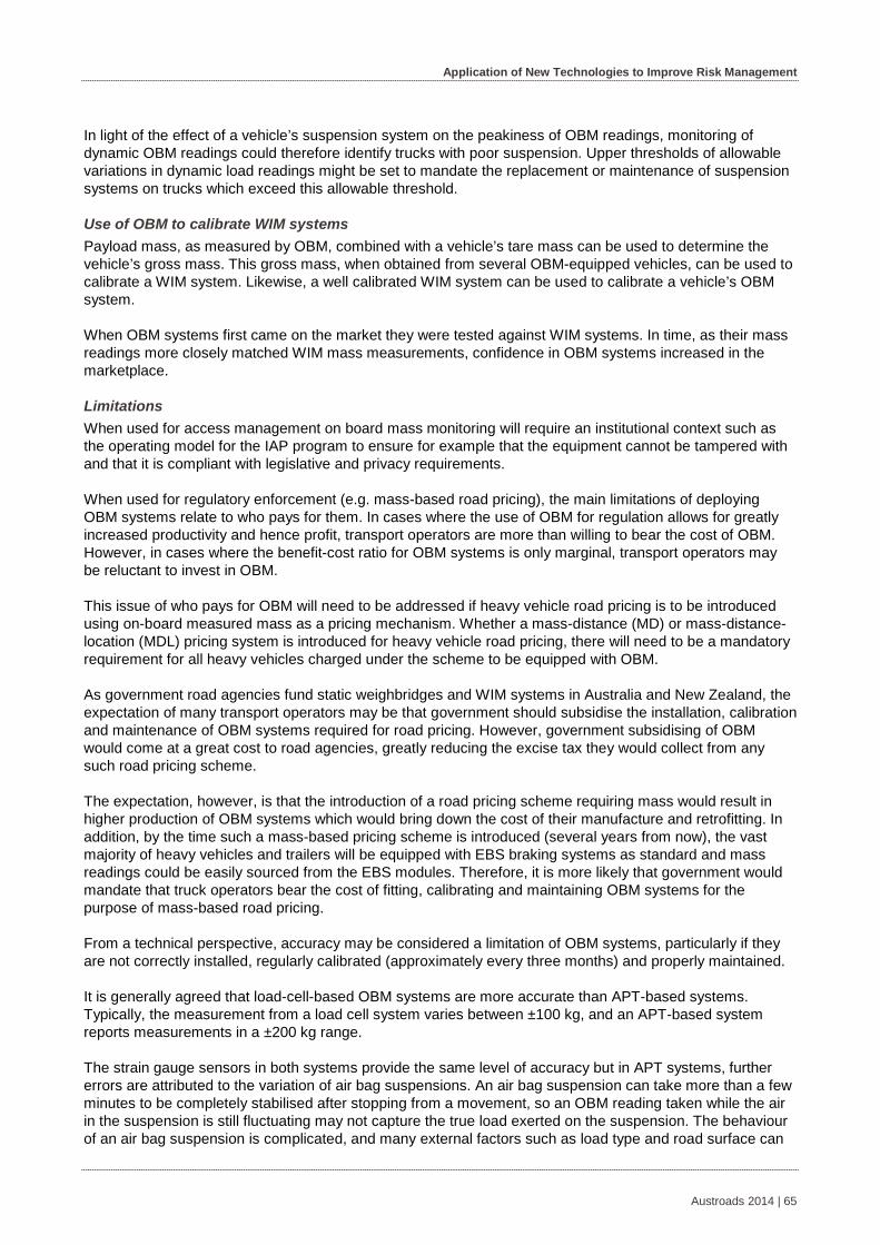
Application of New Technologies to Improve Risk Management
In light of the effect of a vehicle’s suspension system on the peakiness of OBM readings, monitoring of dynamic OBM readings could therefore identify trucks with poor suspension. Upper thresholds of allowable variations in dynamic load readings might be set to mandate the replacement or maintenance of suspension systems on trucks which exceed this allowable threshold.
Use of OBM to calibrate WIM systems Payload mass, as measured by OBM, combined with a vehicle’s tare mass can be used to determine the vehicle’s gross mass. This gross mass, when obtained from several OBM-equipped vehicles, can be used to calibrate a WIM system. Likewise, a well calibrated WIM system can be used to calibrate a vehicle’s OBM system.
When OBM systems first came on the market they were tested against WIM systems. In time, as their mass readings more closely matched WIM mass measurements, confidence in OBM systems increased in the marketplace.
Limitations When used for access management on board mass monitoring will require an institutional context such as the operating model for the IAP program to ensure for example that the equipment cannot be tampered with and that it is compliant with legislative and privacy requirements.
When used for regulatory enforcement (e.g. mass-based road pricing), the main limitations of deploying OBM systems relate to who pays for them. In cases where the use of OBM for regulation allows for greatly increased productivity and hence profit, transport operators are more than willing to bear the cost of OBM. However, in cases where the benefit-cost ratio for OBM systems is only marginal, transport operators may be reluctant to invest in OBM.
This issue of who pays for OBM will need to be addressed if heavy vehicle road pricing is to be introduced using on-board measured mass as a pricing mechanism. Whether a mass-distance (MD) or mass-distance-location (MDL) pricing system is introduced for heavy vehicle road pricing, there will need to be a mandatory requirement for all heavy vehicles charged under the scheme to be equipped with OBM.
As government road agencies fund static weighbridges and WIM systems in Australia and New Zealand, the expectation of many transport operators may be that government should subsidise the installation, calibration and maintenance of OBM systems required for road pricing. However, government subsidising of OBM would come at a great cost to road agencies, greatly reducing the excise tax they would collect from any such road pricing scheme.
The expectation, however, is that the introduction of a road pricing scheme requiring mass would result in higher production of OBM systems which would bring down the cost of their manufacture and retrofitting. In addition, by the time such a mass-based pricing scheme is introduced (several years from now), the vast majority of heavy vehicles and trailers will be equipped with EBS braking systems as standard and mass readings could be easily sourced from the EBS modules. Therefore, it is more likely that government would mandate that truck operators bear the cost of fitting, calibrating and maintaining OBM systems for the purpose of mass-based road pricing.
From a technical perspective, accuracy may be considered a limitation of OBM systems, particularly if they are not correctly installed, regularly calibrated (approximately every three months) and properly maintained.
It is generally agreed that load-cell-based OBM systems are more accurate than APT-based systems. Typically, the measurement from a load cell system varies between ±100 kg, and an APT-based system reports measurements in a ±200 kg range.
The strain gauge sensors in both systems provide the same level of accuracy but in APT systems, further errors are attributed to the variation of air bag suspensions. An air bag suspension can take more than a few minutes to be completely stabilised after stopping from a movement, so an OBM reading taken while the air in the suspension is still fluctuating may not capture the true load exerted on the suspension. The behaviour of an air bag suspension is complicated, and many external factors such as load type and road surface can
Austroads 2014 | 65

Application of New Technologies to Improve Risk Management
significantly affect the time required for it to stabilise. Readings can vary between hill ascents and descents and transient spikes in readings can be generated as the vehicle traverses ruts and hollows on the road.
It is expected that the accuracy of APT-based systems can be improved if more strict procedures are followed.
While the factors mentioned above can affect the accuracy of OBM systems, the degrees of inaccuracy involved may be insignificant if the accuracy levels required for regulatory purposes are relatively low. For example, for a load reading fluctuating about 200 kg, it is still accurate enough if the accuracy of OBM measurements for regulatory purposes needs to be only within a half tonne margin.
Standards/Best Practice 4.2.5An important element of policy for on-board mass technology is how the development of standards is managed. Guiding principles were outlined by the National Transport Commission Strategic Research and Technology Working Group in November 2009 with a recommended focus on facilitating interoperability and minimising the risk of impeding technological innovation.
In summary, the National Transport Commission recommended that:
There is a role for government, through the Draft National In-vehicle Telematics Strategy: The Road Freight Sector (National Transport Commission 2010a), in clarifying the policy framework to allow for the development of systems architecture and communication standards that may support improved levels of interoperability for in-vehicle telematics (including on-board mass) products.
Governments should minimise the imposition of technical product standards that risk stifling innovation. In some circumstances (such as where stricter monitoring of compliance levels is justified) these may be unavoidable.
Through the strategy, the government should support industry in the development of a code of practice. This may provide operators with guidance on how to most effectively utilise in-vehicle telematics in supporting their management of compliance.
To provide a level playing field and to support competition amongst technology developers and suppliers, regulatory on-board mass standards should be developed and maintained in a transparent manner (including publication).
Currently there are no standards in place for OBM systems. However, Transport Certification Australia (TCA) will soon commence type-approval for OBM units (Transport Certification Australia 2013b). This type-approval process will assess OBM units against a nationally-agreed performance-based functional and technical specification to provide transport operators with greater confidence in their use. In addition, type-approval for OBM units will be supported with operational and maintenance guidelines to overcome problems that transport operators have cited in the past regarding the ongoing accuracy, performance and quality of OBM systems.
TCA is currently internally reviewing the performance-based functional and technical specifications as well as the operational and maintenance guidelines before their imminent public release.
Cost of the Technology 4.2.6
Estimated cost figures The cost of various OBM combinations falls principally into three components; the sensors, the indicators and installation cost. APT systems have a significant price differential over load cell systems.
For APT systems, an individual axle group can be fitted with either a single APT fitted to the main airline to the airbags on both sides of the axle, or two APTs in order to monitor each end of the axle.
For mechanical spring suspensions, fifth wheel (turntables), steer axles and trays on rigid trucks, load cells are required. To accurately measure all the deflection axes of an individual axle group, a minimum of two, but more commonly four, load cells are required per axle group.
Austroads 2014 | 66

Application of New Technologies to Improve Risk Management
APTs are relatively easy to fit via tapping off the vehicle’s airline to the suspension, whereas load cells are an integral part of the vehicle and their fitment should ideally be undertaken at the point of assembly of the trailer/axle. While fitment of an APT on an individual axle may take less than an hour, an aftermarket fitment of load cells for an individual axle group may take a couple of days, during which time the vehicle is not working and earning income, imposing a significant and measurable extra cost on such systems.
Table 4.4 provides an indicative cost (as of 2009) of the various systems.
Table 4.4: Indicative costs for different OBM configurations
Vehicle class OBM system configuration Total
Rigid 4 load cells on the tray $6 500–8 000
Rigid 4 load cells on the tray 1 deflection sensor on steer axle
$8 000–10 000
Rigid 1 APT on drive axle 1 deflection sensor on steer axle
$5 000–7 000
Semi-trailer 2 load cells on fifth wheel 4 load cells on trailer axle
$10 000–12 000
Semi-trailer 2 load cells on trailer axle 1 APT on trailer axle
$7 500–9 500
Semi-trailer 1 APT on drive axle 1 APT on trailer axle
$5 000–7 000
B-double 2 load cells on fifth wheel 4 load cells on front trailer axle 4 load cells on rear trailer axle
$15 000–17 000
B-double 2 load cells on fifth wheel 1 APT on front trailer axle 1 APT on rear trailer axle
$9 000–14 000
B-double 1 APT on drive axle 1 APT on front trailer axle 1 APT on rear trailer axle
$7 500–13 000
Source: Transport Certification Australia (2009).
Truck manufacturers in the US and Europe are optioning APT-based OBM systems as part of their original equipment. It is expected that the cost for APT-based OBM systems will fall as demand for these systems increases.
The regulatory uses of OBM such as the Intelligent Access Program or road pricing require institutional arrangements and procedures to ensure that on-board mass monitoring equipment is compliant with the requirements. Additional to the costs for the devices, there are costs involved with the compliance testing and the establishment of the institutional arrangements.
Case Example 4.2.7
Linking OBM to the IAP for high-productivity vehicles The route between Toowoomba and the Port of Brisbane is used for the export of grain to international markets. A round trip is approximately 260 km and around 120 000 tonnes of grain are transported along this route per annum.
Austroads 2014 | 67

Application of New Technologies to Improve Risk Management
Enabling access to high-productivity vehicles means fewer truck trips, less wear and tear on roads, reduced greenhouse gas emissions and big savings for the entire supply chain, including consumers. It was with these savings in mind that state-of-the-art high-productivity performance based standard (PBS) 2B vehicles were introduced to transport grain along this route.
The Queensland Department of Transport and Main Roads (TMR) was concerned about the performance of PBS 2B vehicles (Figure 4.20), their bridge loading effects and road safety implications. ARRB Group was engaged to conduct a route assessment on these roads using PBS principles while the loading effects on bridges were assessed by TMR’s Engineering and Technology Division.
To provide additional assurance to asset owners, Haulmark, with the assistance of Brisbane-based electronic weighing specialists Tramanco, successfully developed a proposal to link OBM to the IAP. Haulmark’s rationale was that the inclusion of OBM reporting in these units, alongside the IAP, provided an enhanced level of axle mass compliance. In addition to assuring asset owners, it also justified a reduction in the bridge live loading factor due to improved load distributions and a reduction in the number of truck trips.
IAP service provider Transtech Driven plays a lead role, monitoring each vehicle’s location and axle group masses whilst in transit and providing the four road owners along the route with assurance these high-productivity vehicles operate in compliance with their route location and axle group mass permit conditions at all times.
Modelling by TMR has indicated that, with the introduction of PBS 2B vehicles fitted with OBM linked to IAP, trips could be slashed by 50%, resulting in a reduction of up to 624 000 truck kilometres. This equates to an estimated saving of approximately 230 000 litres of fuel and a greenhouse emissions reduction of around 490 tonnes or 40%.
Figure 4.20: A PBS 2B heavy vehicle
Source: Transport Certification Australia (2011).
4.3 Non-destructive Evaluation
Introduction 4.3.1Non-destructive evaluation (NDE) technologies typically involve the use of sensors placed on, near or within the structure’s surface to determine the structure’s current:
structural capacity
as-built configuration or presence of defects.
Austroads 2014 | 68
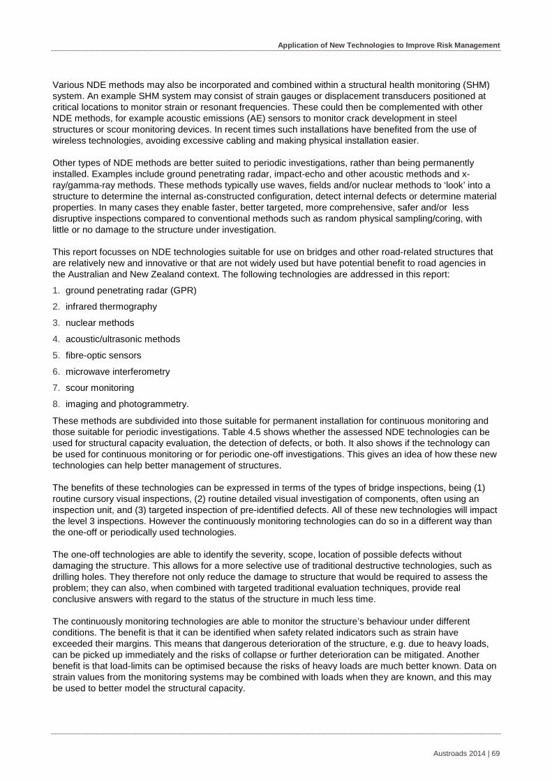
Application of New Technologies to Improve Risk Management
Various NDE methods may also be incorporated and combined within a structural health monitoring (SHM) system. An example SHM system may consist of strain gauges or displacement transducers positioned at critical locations to monitor strain or resonant frequencies. These could then be complemented with other NDE methods, for example acoustic emissions (AE) sensors to monitor crack development in steel structures or scour monitoring devices. In recent times such installations have benefited from the use of wireless technologies, avoiding excessive cabling and making physical installation easier.
Other types of NDE methods are better suited to periodic investigations, rather than being permanently installed. Examples include ground penetrating radar, impact-echo and other acoustic methods and x-ray/gamma-ray methods. These methods typically use waves, fields and/or nuclear methods to ‘look’ into a structure to determine the internal as-constructed configuration, detect internal defects or determine material properties. In many cases they enable faster, better targeted, more comprehensive, safer and/or less disruptive inspections compared to conventional methods such as random physical sampling/coring, with little or no damage to the structure under investigation.
This report focusses on NDE technologies suitable for use on bridges and other road-related structures that are relatively new and innovative or that are not widely used but have potential benefit to road agencies in the Australian and New Zealand context. The following technologies are addressed in this report:
1. ground penetrating radar (GPR)
2. infrared thermography
3. nuclear methods
4. acoustic/ultrasonic methods
5. fibre-optic sensors
6. microwave interferometry
7. scour monitoring
8. imaging and photogrammetry.
These methods are subdivided into those suitable for permanent installation for continuous monitoring and those suitable for periodic investigations. Table 4.5 shows whether the assessed NDE technologies can be used for structural capacity evaluation, the detection of defects, or both. It also shows if the technology can be used for continuous monitoring or for periodic one-off investigations. This gives an idea of how these new technologies can help better management of structures.
The benefits of these technologies can be expressed in terms of the types of bridge inspections, being (1) routine cursory visual inspections, (2) routine detailed visual investigation of components, often using an inspection unit, and (3) targeted inspection of pre-identified defects. All of these new technologies will impact the level 3 inspections. However the continuously monitoring technologies can do so in a different way than the one-off or periodically used technologies.
The one-off technologies are able to identify the severity, scope, location of possible defects without damaging the structure. This allows for a more selective use of traditional destructive technologies, such as drilling holes. They therefore not only reduce the damage to structure that would be required to assess the problem; they can also, when combined with targeted traditional evaluation techniques, provide real conclusive answers with regard to the status of the structure in much less time.
The continuously monitoring technologies are able to monitor the structure’s behaviour under different conditions. The benefit is that it can be identified when safety related indicators such as strain have exceeded their margins. This means that dangerous deterioration of the structure, e.g. due to heavy loads, can be picked up immediately and the risks of collapse or further deterioration can be mitigated. Another benefit is that load-limits can be optimised because the risks of heavy loads are much better known. Data on strain values from the monitoring systems may be combined with loads when they are known, and this may be used to better model the structural capacity.
Austroads 2014 | 69
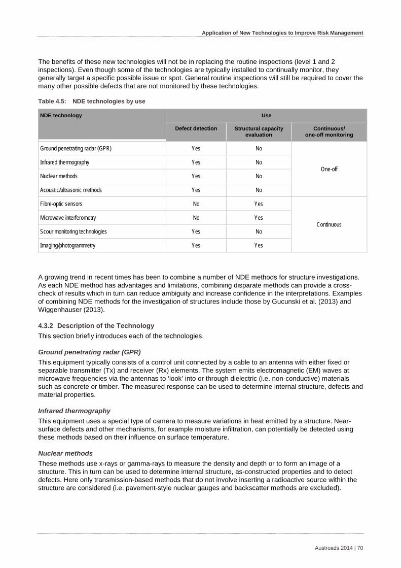
Application of New Technologies to Improve Risk Management
The benefits of these new technologies will not be in replacing the routine inspections (level 1 and 2 inspections). Even though some of the technologies are typically installed to continually monitor, they generally target a specific possible issue or spot. General routine inspections will still be required to cover the many other possible defects that are not monitored by these technologies.
Table 4.5: NDE technologies by use
NDE technology Use
Defect detection Structural capacity evaluation
Continuous/ one-off monitoring
Ground penetrating radar (GPR) Yes No
One-off Infrared thermography Yes No
Nuclear methods Yes No
Acoustic/ultrasonic methods Yes No
Fibre-optic sensors No Yes
Continuous Microwave interferometry No Yes
Scour monitoring technologies Yes No
Imaging/photogrammetry Yes Yes
A growing trend in recent times has been to combine a number of NDE methods for structure investigations. As each NDE method has advantages and limitations, combining disparate methods can provide a cross-check of results which in turn can reduce ambiguity and increase confidence in the interpretations. Examples of combining NDE methods for the investigation of structures include those by Gucunski et al. (2013) and Wiggenhauser (2013).
Description of the Technology 4.3.2This section briefly introduces each of the technologies.
Ground penetrating radar (GPR) This equipment typically consists of a control unit connected by a cable to an antenna with either fixed or separable transmitter (Tx) and receiver (Rx) elements. The system emits electromagnetic (EM) waves at microwave frequencies via the antennas to ‘look’ into or through dielectric (i.e. non-conductive) materials such as concrete or timber. The measured response can be used to determine internal structure, defects and material properties.
Infrared thermography This equipment uses a special type of camera to measure variations in heat emitted by a structure. Near-surface defects and other mechanisms, for example moisture infiltration, can potentially be detected using these methods based on their influence on surface temperature.
Nuclear methods These methods use x-rays or gamma-rays to measure the density and depth or to form an image of a structure. This in turn can be used to determine internal structure, as-constructed properties and to detect defects. Here only transmission-based methods that do not involve inserting a radioactive source within the structure are considered (i.e. pavement-style nuclear gauges and backscatter methods are excluded).
Austroads 2014 | 70
Application of New Technologies to Improve Risk Management
Acoustic/ultrasonic methods These involve the use of transient stress waves (e.g. pressure, shear or surface waves) generated at the structure surface to investigate internal structure, material properties and detect internal defects within structures. There are a range of different techniques using various wave types, equipment and analysis methods. Examples suitable for periodic investigations include ultrasonic pulse velocity, pulse-echo, and impact echo and impact response. These methods are largely focussed on defect detection and material thickness determination. A continuous monitoring example is acoustic emissions (AE), which involves installing a network of acoustic sensors at key locations on the surface of a structure to monitor crack formation and progression, typically used for steel structures.
Fibre-optic sensors Fibre-optic sensors use changes in light to achieve highly sensitive measurements of strain and displacement. Monitoring systems that use these sensors connect via fibre-optic cables to a measuring and data logging device.
Microwave interferometry This non-contact measurement approach involves using electromagnetic waves to measure small movements and resonant frequencies of a structure subject to dynamic loading/effects. The interferometer device is typically positioned in a fixed location and simply pointed at the structure to undertake the measurements.
Scour monitoring Scour is a major cause in many bridge failures and damage to piers and abutments. These use sensors and mechanical set-ups to monitor the loss of material adjacent to piers, piles and abutments during flood events. A typical fixed scour monitoring system includes sensors, data loggers and a data transfer system. The selection of sensors is based on various sensors and site attributes. The sensors may be connected to the data logger(s) by a wired or wireless connection.
Photogrammetry Close range photogrammetry cameras are used to model buildings, engineering structures, vehicles, forensic and accident scenes. Typically, a camera is hand held or set on a tripod close to the subject and a 3D model or a drawing is produced. Stereo photogrammetry estimates 3D coordinates of points on an object. Common points are identified on each image and a line of sight can be constructed from the camera location to these points on the object.
Potentially the following measurements can be made on the bridge structures using photogrammetric technologies (Jáuregui et al. 2003):
as-built bridge geometry
settlement and temperature-induced deflections
live load and dead load deflections
initial camber of bridge girders
damage and deterioration such as crack width, section loss, spalling and delamination, etc.
Physical Principles 4.3.3This section describes the physical principles for each technology.
Ground penetrating radar (GPR) GPR equipment emits pulsed or continuously modulated electromagnetic (EM) signals into the concrete or timber structure using an antenna placed on or near the material surface. EM waves emitted into this material propagate according to Maxwell’s equations and partially reflect when they encounter a change in intrinsic impedance, typically at the boundary of contrasting material types (e.g. concrete-air, concrete-water, etc.), with the magnitude and phase of the reflection depending on the material contrast. The reflected
Austroads 2014 | 71
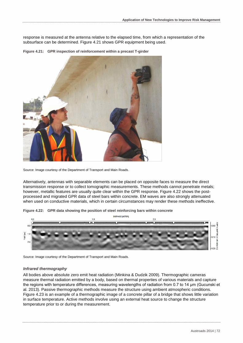
Application of New Technologies to Improve Risk Management
response is measured at the antenna relative to the elapsed time, from which a representation of the subsurface can be determined. Figure 4.21 shows GPR equipment being used.
Figure 4.21: GPR inspection of reinforcement within a precast T-girder
Source: Image courtesy of the Department of Transport and Main Roads.
Alternatively, antennas with separable elements can be placed on opposite faces to measure the direct transmission response or to collect tomographic measurements. These methods cannot penetrate metals; however, metallic features are usually quite clear within the GPR response. Figure 4.22 shows the post-processed and migrated GPR data of steel bars within concrete. EM waves are also strongly attenuated when used on conductive materials, which in certain circumstances may render these methods ineffective.
Figure 4.22: GPR data showing the position of steel reinforcing bars within concrete
Source: Image courtesy of the Department of Transport and Main Roads.
Infrared thermography All bodies above absolute zero emit heat radiation (Minkina & Dudzik 2009). Thermographic cameras measure thermal radiation emitted by a body, based on thermal properties of various materials and capture the regions with temperature differences, measuring wavelengths of radiation from 0.7 to 14 μm (Gucunski et al. 2013). Passive thermographic methods measure the structure using ambient atmospheric conditions. Figure 4.23 is an example of a thermographic image of a concrete pillar of a bridge that shows little variation in surface temperature. Active methods involve using an external heat source to change the structure temperature prior to or during the measurement.
Austroads 2014 | 72

Application of New Technologies to Improve Risk Management
Figure 4.23: Thermographic image of a concrete bridge column
Source: Image courtesy of the Department of Transport and Main Roads.
Nuclear methods Nuclear methods can be divided into two groups – radiometric methods and radiographic methods (American Concrete Institute 1998). Radiometry, also known as ‘gauging’, involves measuring the average intensity of x-ray or gamma-rays passing through a material for a given time. Based on the measured intensity and known thickness, the average material density can be determined. Alternatively for a known material density its thickness can be determined. Radiography involves creating an image of transmitted intensity using a sheet of film or an electronic detector. Figure 4.24 shows a trial of gamma-ray gauging to detect internal defects within recovered timber bridge girders. A C-shaped frame is use to keep the radioactive isotope (below the girder) a fixed distance from an electronic detector, which connects to a nearby laptop to display transmitted radiation intensity.
Figure 4.24: Trial of gamma-ray gauging to detect defects in timber bridge girders
Source: Image courtesy of the Department of Transport and Main Roads.
Austroads 2014 | 73

Application of New Technologies to Improve Risk Management
Either x-rays or gamma-rays can be used for the radioactive source. While x-rays can be generated, gamma-rays are produced by a decaying radioactive isotope and so can be smaller/lighter. The radiation source is typically collimated, that is the emissions are directed in a narrow stream towards the detector, to minimise stray emissions. There is inherent safety, licensing, and in the case of gamma-rays, disposal issues with these methods that add to the cost of surveys.
Acoustic/ultrasonic methods Ultrasonic pulse velocity (UPV) – involves placing ultrasonic transducers, typically piezoelectric, on the material surface at a known spacing to measure the velocity of pressure (P-waves) and/or surface waves (Raleigh) in the frequency range 20–300 kHz, typically 24 or 54 kHz (Garnier in Breysse 2012, p. 18). Direct, semi-direct and indirect configurations can be used for the measurement. The measured velocity can be used to estimate dynamic modulus of elasticity (Ed), which in turn may be related to the compressive strength (fc) of concrete samples, however it is difficult or impossible to relate UPV measurements to absolute strength of in situ concrete (Bungey, Millard & Grantham 2006). Reductions in pulse velocity can also be used to detect honeycombed or poorly compacted concrete.
Ultrasonic pulse echo – measures the time of flight of P-waves or shear waves (S-waves) in the frequency range 20 kHz-300 kHz to detect internal interfaces and defects (Krause & Mielentz 2012). Waves are generated and detected using arrays of piezoelectric transducers placed on the material surface. Transit and reflection time of ultrasonic waves within the material are used to indirectly detect the presence of internal flaws such as cracking, voids, delamination/horizontal cracking which exhibit as differences in acoustic impedance (Gucunski et al. 2013). Synthetic aperture focussing techniques can then be used to generate 2D and 3D representations within the material.
Impact echo – this technique is used for flaw detection within concrete (Carino 2001). The method involves striking the surface to create stress waves and then measuring the response nearby. It is primarily used to detect delamination in concrete based on detecting wave reflectors or ‘resonators’ within structural elements (Gucunski et al. 2013). Stress waves travelling within concrete almost totally reflect when they encounter an interface with air (Carino 2001). The depth to these interfaces can be estimated from the frequency of the reflections and the measured or estimated compression-wave velocity of concrete (Gucunski et al. 2013), in which delamination appears as shallow reflectors (i.e. high-frequency peaks) within the frequency spectrum of the measured response. Impact echo measurements typically operate in a frequency range between 3 to 40 kHz (Gucunski et al. 2013).
Impulse response – this method involves impacting the surface of the structure with a hammer and measuring the resulting response with a nearby transducer, geophone or accelerometer, using the ratio of the displacement and impact frequency spectrum (Gucunski et al. 2013). The method differs from impact echo in that it uses a lower frequency spectrum (0 to1 kHz) and focusses more on the structural response of the surface itself rather than the propagation time of waves (Gucunski et al.2013).
Acoustic emissions (AE) – this a passive NDE method involving monitoring of acoustic signals arising from the rapid release of strain energy due to micro-structural changes within a material due to the initiation and/or growth of cracks, yielding, bond failure, fibre failure and delamination in composites. Based on the difference in arrival times of these signals at AE sensors placed at different locations, the location of these defects can be estimated.
Fibre-optic sensors Fibre-optic monitoring systems include fibre-optic sensors (FOS), fibre-optic cables and a measuring device. When in operation, a light beam is sent through the cables to the sensors and is modulated according to the amount of the change in length of the sensor. The sensor reflects back an optical signal to the measuring device which translates the reflected light into numerical measurements of the change in sensor length.
Austroads 2014 | 74
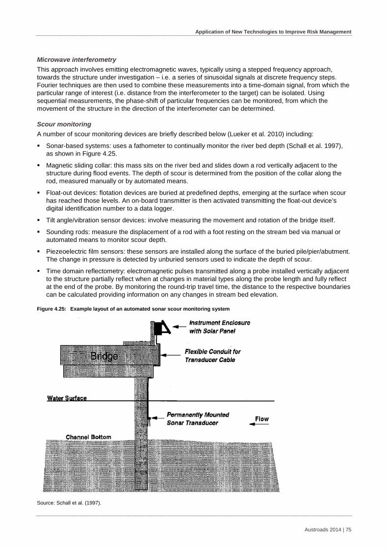
Application of New Technologies to Improve Risk Management
Microwave interferometry This approach involves emitting electromagnetic waves, typically using a stepped frequency approach, towards the structure under investigation – i.e. a series of sinusoidal signals at discrete frequency steps. Fourier techniques are then used to combine these measurements into a time-domain signal, from which the particular range of interest (i.e. distance from the interferometer to the target) can be isolated. Using sequential measurements, the phase-shift of particular frequencies can be monitored, from which the movement of the structure in the direction of the interferometer can be determined.
Scour monitoring A number of scour monitoring devices are briefly described below (Lueker et al. 2010) including:
Sonar-based systems: uses a fathometer to continually monitor the river bed depth (Schall et al. 1997), as shown in Figure 4.25.
Magnetic sliding collar: this mass sits on the river bed and slides down a rod vertically adjacent to the structure during flood events. The depth of scour is determined from the position of the collar along the rod, measured manually or by automated means.
Float-out devices: flotation devices are buried at predefined depths, emerging at the surface when scour has reached those levels. An on-board transmitter is then activated transmitting the float-out device’s digital identification number to a data logger.
Tilt angle/vibration sensor devices: involve measuring the movement and rotation of the bridge itself.
Sounding rods: measure the displacement of a rod with a foot resting on the stream bed via manual or automated means to monitor scour depth.
Piezeoelectric film sensors: these sensors are installed along the surface of the buried pile/pier/abutment. The change in pressure is detected by unburied sensors used to indicate the depth of scour.
Time domain reflectometry: electromagnetic pulses transmitted along a probe installed vertically adjacent to the structure partially reflect when at changes in material types along the probe length and fully reflect at the end of the probe. By monitoring the round-trip travel time, the distance to the respective boundaries can be calculated providing information on any changes in stream bed elevation.
Figure 4.25: Example layout of an automated sonar scour monitoring system
Source: Schall et al. (1997).
Austroads 2014 | 75
Application of New Technologies to Improve Risk Management
Photogrammetry Photogrammetry determines geometric properties of objects from photographic images. This is a non-contact, non-destructive SHM technique in which 3D measurements are determined based on two-dimensional photographs taken of an object. At least two camera positions are used in the survey. From each camera position, there is a line of sight that runs from each point on the object to the perspective centre of the camera. Using the principle of triangulation, the point of intersection between the different lines of sight for a particular point is determined mathematically to identify the spatial or 3D location of the object point. The changes in the 3D location of the object point obtained from two sets of photographs before and after the event will give the resulting displacement of the object point.
Use and Limitations 4.3.4This section describes the possible uses of the technologies and limitations of the technologies.
Ground penetrating radar (GPR) GPR is well suited for detecting embedded features within concrete such as reinforcing bars or conduits, internal defects (e.g. voids and honeycombing) and detecting variations in wall thickness. As the technique relies on EM waves reflecting from material contrasts, features can only be detected if they contrast sufficiently with surrounding materials. Consequently GPR is not well suited to detecting thin cracks or delamination, particularly those that run parallel to the surface being scanned. Similarly, it is not well suited to detecting boundaries of similar material types (e.g. a join of two concrete pours). However, in some cases it is possible to detect larger cracks that are transverse to the direction of scanning, particularly if they are filled with a contrasting dielectric (e.g. water-filled cracks in concrete). Localised cracking and deterioration may also be detectable where damage has progressed to a point that the affected region contrasts with the surrounding material. Another issue for GPR is that the EM waves can be severely attenuated due to increases of ionic conductivity, for example wet concrete with chloride-ingress. However, this disadvantage can be turned into a benefit, by using increases in signal attenuation as a means of identifying areas affected by chloride ingress.
As with concrete, GPR is best suited to detecting material contrasts within timber and so is well suited to detecting larger internal features (e.g. internal holes, rot) or responses from strong reflectors such as embedded metal bolts. When used on timber girders the GPR approach is fast and non-destructive. The practical aspects of these investigations are outlined in Riggio et al. (2013). GPR, unlike ultrasound, is not severely attenuated by cracks. For timber this can be an advantage as old timber girders typically have many cracks, which limits the penetration depth of acoustic/ultrasonic methods. Of course this also means GPR is not well suited to detecting those cracks, except where they form a sufficiently large zone which effectively forms a dielectric contrast to the surrounding timber. An additional consideration is that moisture has a strong influence on the GPR response, generally leading to a slowing of EM waves. As noted by Muller et al. (2010) this also provides a means of identifying internal moisture ingress within timber girders of a consistent diameter.
Infrared thermography Active infrared thermography methods use an artificial source to heat the structure whereas passive methods measure the structure at its ambient conditions. In practice, passive methods are far simpler and more likely to be used for road structures. However, this approach is strongly influenced by the sun, air temperature, shadows, time of the day, etc. Furthermore, the geometry of the structure can also result in variations of emitted heat towards the camera (e.g. cylindrical columns v. flat headstocks etc.). Moisture ingress can also have a significant influence on surface temperature, which can enable thermography to detect its effect. Although data collection is quick and relatively easy, various factors need to be taken into consideration when assessing the suitability of thermography for a particular investigation/application.
Austroads 2014 | 76

Application of New Technologies to Improve Risk Management
Nuclear methods In practice, the use of nuclear methods is relatively rare for concrete and timber investigations, most likely due to a combination of safety concerns, expense and practicality issues. A key issue is that these methods pose a safety risk to operators and the general public because of the use of ionising radiation. Operators require licensing and in the case of gamma-ray methods, the equipment must be regularly calibrated due to continual degradation of the isotope. In addition, as isotope disposal (i.e. at the end of its useful life) is expensive, these costs must also be factored into equipment hire/purchase costs. These issues all add to the cost and complexity of site investigations. However, in certain critical or high value situations, nuclear methods may be the only means that will work and so should remain in the toolkit of available NDE methods.
Acoustic/ultrasonic methods Ultrasonic pulse velocity (UPV) – is often used as a rapid, non-destructive method of assessing concrete quality and estimating elastic modulus based on the velocity of wave propagation. A related technique, cross-hole sonic logging (CSL), can be used as a rapid method of assessing early-age concrete quality for bored piles by measuring travel time between a pair of geophones lowered into PVC ducts cast on opposite sides of the inner face of circumferential reinforcing. Typically, four 50 mm PVC ducts are installed in a cross pattern, which are filled with water for the measurement.
Ultrasonic pulse echo – recent versions of this equipment use an array of spring-loaded dry-point contact piezoelectric transducers placed on the surface to emit and receive shear waves and then use the synthetic aperture focussing technique (SAFT) to generate 2D and 3D representations of the subsurface. The measurements can be used to detect internal objects, interfaces and anomalies (Gucunski et al. 2013). This equipment is distributed within Australia by PCTE (www.pcte.com.au) and is often used to detect flaws and interfaces within concrete. The key advantage of this approach, compared with GPR, is the ability to see through closely spaced reinforcing. Like other acoustic/ultrasonic methods this method requires static positioning of transducers during the measurement, limiting the rate of data collection/coverage.
Impact echo – this technique is well suited to detecting thin delamination that would be too small to detect using GPR. It requires good contact of the transducer with the concrete surface. In practice, several ‘hits’ of the concrete surface may be required to get a valid response. Like other acoustic/ultrasonic methods this method requires static positioning of transducers during the measurement, limiting the rate of data collection/coverage.
Impulse response – this approach is best suited to detecting concrete delamination, though it has traditionally been used in road investigations focussing on deeper investigations. Like other acoustic/ultrasonic methods this method requires static positioning of transducers during the measurement, limiting the rate of data collection/coverage.
Acoustic emissions (AE) – these systems are best suited for continuous monitoring of damage growth within steel structures. These methods become impractical for concrete, due to the higher signal attenuation. Furthermore, issues with noise and the ability to discriminate AE events requires specialist expertise for interpretation of the results.
Fibre-optic sensors As fibre-optic sensors are made of non-conductive material, they can be used when electromagnetic and radio frequency interference are an issue. There is long-term stability to noise or signal loss due to connector and lead wire resistance; they are capable of intermittent readings with no reconnection errors and they are non-corrosive, embeddable and easy to be bonded to most materials. This means they are flexible to be applied in any structural shape with different lengths of sensors. Disadvantages are the high installation costs, the susceptibility to physical damage and often special test equipment is required.
Austroads 2014 | 77

Application of New Technologies to Improve Risk Management
Different types of FOS are suitable for different types of structures:
Short gauge FOS are suitable to measure local material behaviour while long gauge FOS are suitable to measure global behaviour of the structure. SG sensors are also good to measure crack widths of existing cracks. Some FOS also exist in strain rosettes that are useful when there is a need to measure in several directions.
Long gauge FOS are suitable to either cast in concrete or to be mounted on the concrete surface as long as they are not in direct sunlight as this may affect the measurements. These sensors provide measurements in concrete from early age to long-term measurements with excellent long-term stability but are also suitable for steel and composite materials.
Distributed FOS is suitable for large structures such as bridges, pipelines, dams, roads, pavements and various geotechnical applications. They measure distributed strain, temperature and can also be used for crack detection, localisation and crack width measurements. This system can replace a large number of discrete sensors as a single cable and is sensitive at every point along its length.
Microwave interferometry This is a highly sensitive and precise measurement method best suited to measuring small movements in the direction of the interferometer. As the measurements are repeated at a rapid rate the approach is also suitable for non-contact measurement of resonant frequencies. However there are several practical issues to be considered. For one, limits on the range of frequencies that can be emitted by the device limit its time domain resolution. The practical effect is that the interferometer can only distinguish points in approximately 0.75 m steps apart. Special microwave reflectors need to be installed at key measurement points, to ensure the phase-shift of those points dominates at the measurement time of interest. It is often difficult to determine which point is which within the return signal, however this can be determined by physically moving the reflectors to see which point moves within a test measurement. Furthermore, components of unwanted structure movement can affect the readings. For example, Figure 4.26 shows a typical set-up, which assumes the component measured by the interferometer is due to vertical displacement of the girder. However, a horizontal translation of the girder may produce a similar effect from the viewpoint of the interferometer.
Figure 4.26: Microwave interferometry test set-up for bridge monitoring
Source: Pieraccini (2013).
Scour monitoring The use of scour monitoring technologies is self-evident. Scour is a major cause in many bridge failures and damage to piers and abutments. In most cases, scour is not easily noticeable in underwater conditions. In these cases, monitoring of bed levels at each pier and abutment location should be a required maintenance activity.
Austroads 2014 | 78

Application of New Technologies to Improve Risk Management
Photogrammetry Photogrammetry can be used where traditional instruments cannot be used as no fixed bases can be provided due to difficult access conditions under the bridge. It is capable of non-contact measuring spatial coordinates (in three dimensions) of discrete points on the structure.
A disadvantage is that performance of the photogrammetry procedure may be affected by the environmental conditions like seasonal weather patterns that produce increased wind and cloud cover, shadows and sun spots caused by solar conditions, dense vegetation, snow, overhangs and water.
Standards/Best Practice 4.3.5A list of guidebooks, conference proceedings and review papers regarding the use of NDE methods is provided below. There is a wide range of international standards in use regarding these methods, details of which can be found in the listed sources.
General
Manuals/guides PIARC (2012), Inspector accreditation, non-destructive testing and condition assessment for bridges,
report 2011R07, PIARC Technical Committee D3 Road Bridges, PIARC/World Road Association, Paris, France.
Highways Agency (2006), Design manual for roads and bridges: volume 3: part 7: advice notes on the non-destructive testing of highway structures, BA86/06, Highways Agency, London, UK.
Conference proceedings Non-destructive Testing in Civil Engineering (NDT-CE)
– International symposium on non-destructive testing in civil engineering NDT-CE 2003, 6th, Berlin, Germany, DZGIP, Berlin, Germany, viewed 31 October 2013, <http://www.ndt.net/article/ndtce03/index.htm>.
— International symposium on non-destructive testing in civil engineering NDT-CE 2009, 7th, Nantes, France, LCPC, Paris, France, viewed 31 October 2013, <http://www.ndt.net/article/ndtce2009/toc.htm>.
RILEM symposium RILEM symposium on on-site assessment of concrete, masonry and timber structures: SACoMaTiS
2008, 1st, Varenna, Italy, RILEM, Bagneux, France, viewed 31 October 2013, <http://www.rilem.org/gene/main.php?base=500218&id_publication=63>.
Structural Faults and Repair Biennial International Conferences 1987 onwards.
Concrete structures American Concrete Institute (1998), Non-destructive test methods for evaluation of concrete in structures,
report ACI 228.2R-98, ACI, Farmington Hills, MI, USA.
Breysse, D (ed) (2012), Non-destructive assessment of concrete structures: reliability and limits of single and combined techniques, RILEM State-of-the-Art Reports, vol. 1, Springer, Netherlands.
Concrete Society (1997), Guidance on the radar testing of concrete structures, technical report 48, Concrete Society, Camberley, UK.
Gucunski, N, Imani, A, Romero, F, Nazarian, S, Yuan, D, Wiggenhauser, H, Shokouhi, P, Taffe, A and Kutrubes, D (2013), Nondestructive testing to identify concrete bridge deck deterioration, SHRP 2 report S2-R06A-RR-1, Transportation Research Board, Washington, DC, USA.
International Atomic Energy Agency (2002), Guidebook on non-destructive testing of concrete structures, training course series 17, IAE, Vienna, Austria.
Austroads 2014 | 79

Application of New Technologies to Improve Risk Management
Maierhofer, C, Reinhardt, HW and Dobmann, G (eds) (2010), Non-destructive evaluation of reinforced
concrete structures: volume 2: non-destructive testing methods, CRC Press, Boca Raton, Florida, USA.
Malhotra, VM and Carino, NJ (2003), Handbook on non-destructive testing of concrete, 2nd edn, CRC Press, Boca Raton, Florida, USA.
Wimsatt, A, White J, Leung, C, Scullion, T, Hurlebaus, S et al. (2013), Mapping voids, debonding, delaminations, moisture and other defects behind or within tunnel linings, SHRP 2 renewal project R06G, Transportation Research Board, Washington, DC, USA.
Timber structures RILEM Technical Committee 215-AST Insitu Assessment Of Structural Timber
– Kasal, B and Tannert, T (eds) (2010), In situ assessment of structural timber, RILEM State-of-the-Art Reports, vol. 7, Springer, Netherlands.
– Tannert T, Kasal, B and Anthony, R (2010), ‘RILEM TC 215 insitu assessment of structural timber: report on activities and application of assessment methods’, in Ceccotti, A (ed), 11th World conference on timber engineering 2010 (WCTE 2010), Trees and Timber Institute, National Research Council, Toscana, Italy, pp. 642-8.
– Riggio, M, Anthony, RW, Augelli, F, Kasal, B, Lechner, T, Muller, W and Tannert, T (2013), ‘In situ assessment of structural timber using non-destructive techniques’, Materials and Structures, July, 18 pp.
— Dietsch, P and Köhler, J (eds) (2010), Assessment of timber structures, COST action E55, Shaker, Germany.
Cost of the Technology 4.3.6There are three main components that determine the total costs of applying these technologies, being:
the costs for the technology (hardware and software)
the costs for the installation or execution of the surveys
the costs for the processing of the data.
The cost of a survey does not only depend on the technology, but also on local conditions like the size of the structure and the accessibility. Depending on the technology, the three main components can be fixed or variable with the size of the structure. Also, for some technologies different levels of analysis can be performed on the data. Additionally, as these technologies are constantly evolving the associated costs involved are constantly being reduced. Therefore, no absolute costs are provided. Table 4.6 provides comments on the factors influencing the costs, as well as a rough relative indication of the total survey cost, or in the case of a continuously monitoring technology, the total roll-out costs for the complete life cycle. This includes the costs for the technology, the installation and the processing of the data.
Austroads 2014 | 80
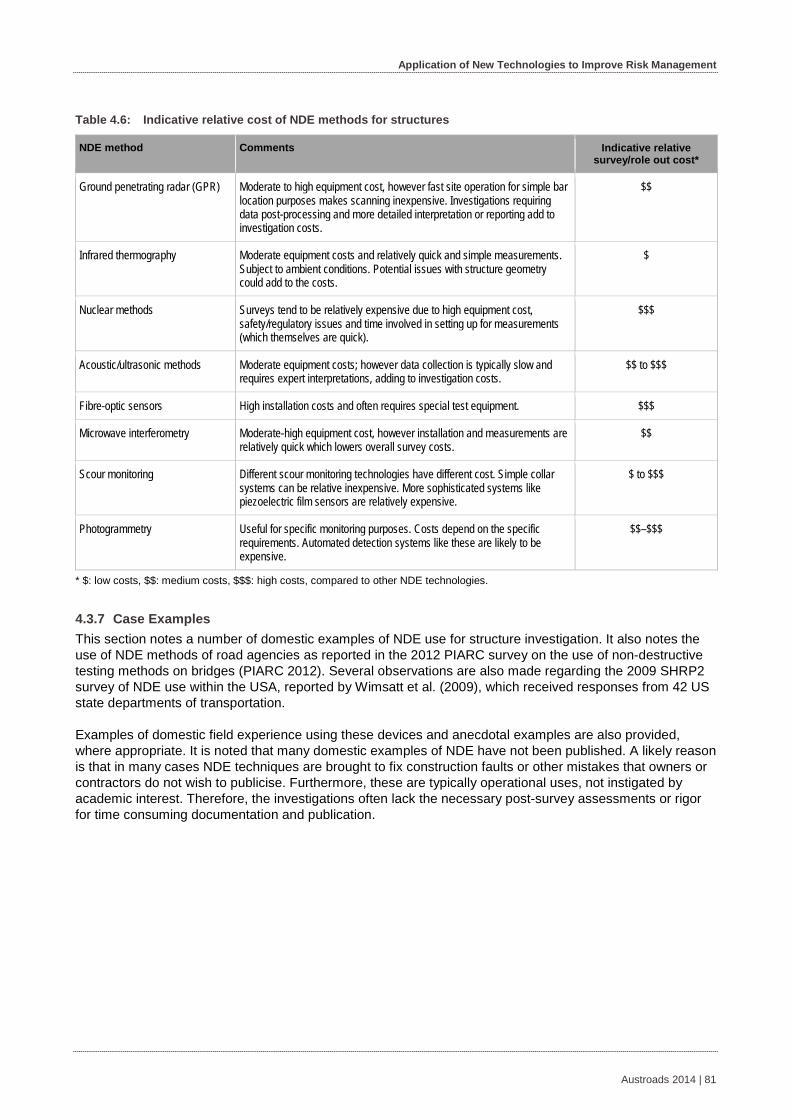
Application of New Technologies to Improve Risk Management
Table 4.6: Indicative relative cost of NDE methods for structures
NDE method Comments Indicative relative survey/role out cost*
Ground penetrating radar (GPR) Moderate to high equipment cost, however fast site operation for simple bar location purposes makes scanning inexpensive. Investigations requiring data post-processing and more detailed interpretation or reporting add to investigation costs.
$$
Infrared thermography Moderate equipment costs and relatively quick and simple measurements. Subject to ambient conditions. Potential issues with structure geometry could add to the costs.
$
Nuclear methods Surveys tend to be relatively expensive due to high equipment cost, safety/regulatory issues and time involved in setting up for measurements (which themselves are quick).
$$$
Acoustic/ultrasonic methods Moderate equipment costs; however data collection is typically slow and requires expert interpretations, adding to investigation costs.
$$ to $$$
Fibre-optic sensors High installation costs and often requires special test equipment. $$$
Microwave interferometry Moderate-high equipment cost, however installation and measurements are relatively quick which lowers overall survey costs.
$$
Scour monitoring Different scour monitoring technologies have different cost. Simple collar systems can be relative inexpensive. More sophisticated systems like piezoelectric film sensors are relatively expensive.
$ to $$$
Photogrammetry Useful for specific monitoring purposes. Costs depend on the specific requirements. Automated detection systems like these are likely to be expensive.
$$–$$$
* $: low costs, $$: medium costs, $$$: high costs, compared to other NDE technologies.
Case Examples 4.3.7This section notes a number of domestic examples of NDE use for structure investigation. It also notes the use of NDE methods of road agencies as reported in the 2012 PIARC survey on the use of non-destructive testing methods on bridges (PIARC 2012). Several observations are also made regarding the 2009 SHRP2 survey of NDE use within the USA, reported by Wimsatt et al. (2009), which received responses from 42 US state departments of transportation.
Examples of domestic field experience using these devices and anecdotal examples are also provided, where appropriate. It is noted that many domestic examples of NDE have not been published. A likely reason is that in many cases NDE techniques are brought to fix construction faults or other mistakes that owners or contractors do not wish to publicise. Furthermore, these are typically operational uses, not instigated by academic interest. Therefore, the investigations often lack the necessary post-survey assessments or rigor for time consuming documentation and publication.
Austroads 2014 | 81
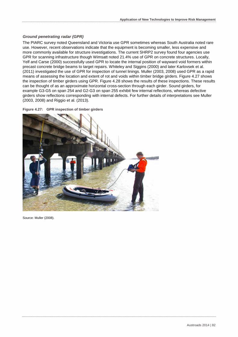
Application of New Technologies to Improve Risk Management
Ground penetrating radar (GPR) The PIARC survey noted Queensland and Victoria use GPR sometimes whereas South Australia noted rare use. However, recent observations indicate that the equipment is becoming smaller, less expensive and more commonly available for structure investigations. The current SHRP2 survey found four agencies use GPR for scanning infrastructure though Wimsatt noted 21.4% use of GPR on concrete structures. Locally, Yelf and Carse (2000) successfully used GPR to locate the internal position of wayward void formers within precast concrete bridge beams to target repairs. Whiteley and Siggins (2000) and later Karlovsek et al. (2011) investigated the use of GPR for inspection of tunnel linings. Muller (2003, 2008) used GPR as a rapid means of assessing the location and extent of rot and voids within timber bridge girders. Figure 4.27 shows the inspection of timber girders using GPR. Figure 4.28 shows the results of these inspections. These results can be thought of as an approximate horizontal cross-section through each girder. Sound girders, for example G3-G5 on span 254 and G2-G3 on span 255 exhibit few internal reflections, whereas defective girders show reflections corresponding with internal defects. For further details of interpretations see Muller (2003, 2008) and Riggio et al. (2013).
Figure 4.27: GPR inspection of timber girders
Source: Muller (2008).
Austroads 2014 | 82
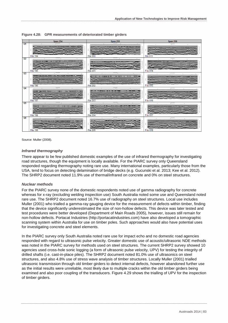
Application of New Technologies to Improve Risk Management
Figure 4.28: GPR measurements of deteriorated timber girders
Source: Muller (2008).
Infrared thermography There appear to be few published domestic examples of the use of infrared thermography for investigating road structures, though the equipment is locally available. For the PIARC survey only Queensland responded regarding thermography noting rare use. Many international examples, particularly those from the USA, tend to focus on detecting delamination of bridge decks (e.g. Gucunski et al. 2013; Kee et al. 2012). The SHRP2 document noted 11.9% use of thermal/infrared on concrete and 0% on steel structures.
Nuclear methods For the PIARC survey none of the domestic respondents noted use of gamma radiography for concrete whereas for x-ray (excluding welding inspection use) South Australia noted some use and Queensland noted rare use. The SHRP2 document noted 16.7% use of radiography on steel structures. Local use includes Muller (2001) who trialled a gamma-ray gauging device for the measurement of defects within timber, finding that the device significantly underestimated the size of non-hollow defects. This device was later tested and test procedures were better developed (Department of Main Roads 2005), however, issues still remain for non-hollow defects. Portacat Industries (http://portacatindustries.com) have also developed a tomographic scanning system within Australia for use on timber poles. Such approaches would also have potential uses for investigating concrete and steel elements.
In the PIARC survey only South Australia noted rare use for impact echo and no domestic road agencies responded with regard to ultrasonic pulse velocity. Greater domestic use of acoustic/ultrasonic NDE methods was noted in the PIARC survey for methods used on steel structures. The current SHRP2 survey showed 10 agencies used cross-hole sonic logging (a form of ultrasonic pulse velocity, UPV) for testing the integrity of drilled shafts (i.e. cast-in-place piles). The SHRP2 document noted 81.0% use of ultrasonics on steel structures, and also 4.8% use of stress wave analysis of timber structures. Locally Muller (2001) trialled ultrasonic transmission through old timber girders to detect internal defects, however abandoned further use as the initial results were unreliable, most likely due to multiple cracks within the old timber girders being examined and also poor coupling of the transducers. Figure 4.29 shows the trialling of UPV for the inspection of timber girders.
Austroads 2014 | 83
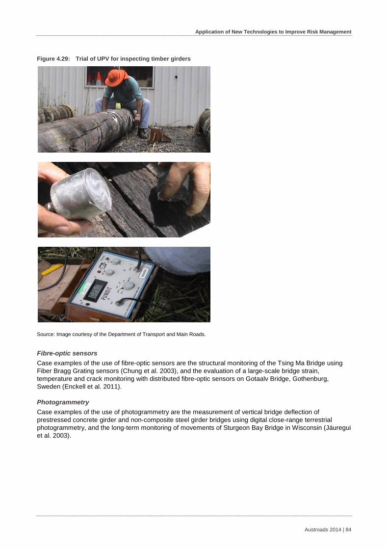
Application of New Technologies to Improve Risk Management
Figure 4.29: Trial of UPV for inspecting timber girders
Source: Image courtesy of the Department of Transport and Main Roads.
Fibre-optic sensors Case examples of the use of fibre-optic sensors are the structural monitoring of the Tsing Ma Bridge using Fiber Bragg Grating sensors (Chung et al. 2003), and the evaluation of a large-scale bridge strain, temperature and crack monitoring with distributed fibre-optic sensors on Gotaalv Bridge, Gothenburg, Sweden (Enckell et al. 2011).
Photogrammetry Case examples of the use of photogrammetry are the measurement of vertical bridge deflection of prestressed concrete girder and non-composite steel girder bridges using digital close-range terrestrial photogrammetry, and the long-term monitoring of movements of Sturgeon Bay Bridge in Wisconsin (Jáuregui et al. 2003).
Austroads 2014 | 84
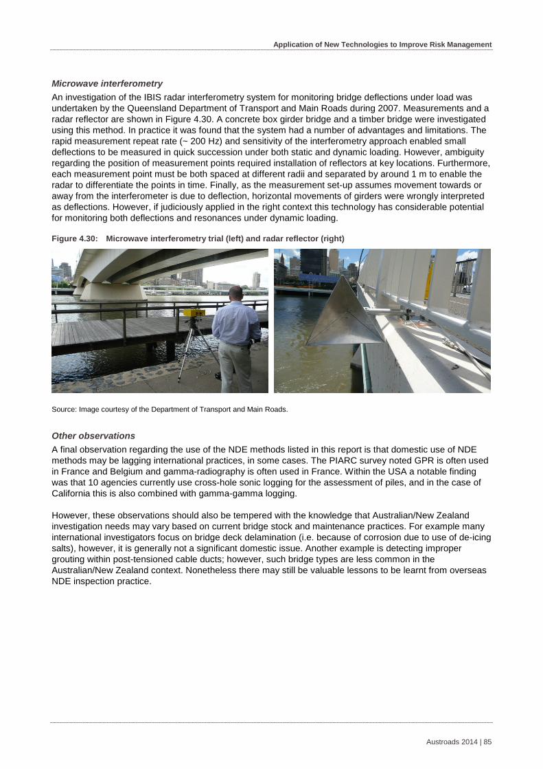
Application of New Technologies to Improve Risk Management
Microwave interferometry An investigation of the IBIS radar interferometry system for monitoring bridge deflections under load was undertaken by the Queensland Department of Transport and Main Roads during 2007. Measurements and a radar reflector are shown in Figure 4.30. A concrete box girder bridge and a timber bridge were investigated using this method. In practice it was found that the system had a number of advantages and limitations. The rapid measurement repeat rate (~ 200 Hz) and sensitivity of the interferometry approach enabled small deflections to be measured in quick succession under both static and dynamic loading. However, ambiguity regarding the position of measurement points required installation of reflectors at key locations. Furthermore, each measurement point must be both spaced at different radii and separated by around 1 m to enable the radar to differentiate the points in time. Finally, as the measurement set-up assumes movement towards or away from the interferometer is due to deflection, horizontal movements of girders were wrongly interpreted as deflections. However, if judiciously applied in the right context this technology has considerable potential for monitoring both deflections and resonances under dynamic loading.
Figure 4.30: Microwave interferometry trial (left) and radar reflector (right)
Source: Image courtesy of the Department of Transport and Main Roads.
Other observations A final observation regarding the use of the NDE methods listed in this report is that domestic use of NDE methods may be lagging international practices, in some cases. The PIARC survey noted GPR is often used in France and Belgium and gamma-radiography is often used in France. Within the USA a notable finding was that 10 agencies currently use cross-hole sonic logging for the assessment of piles, and in the case of California this is also combined with gamma-gamma logging.
However, these observations should also be tempered with the knowledge that Australian/New Zealand investigation needs may vary based on current bridge stock and maintenance practices. For example many international investigators focus on bridge deck delamination (i.e. because of corrosion due to use of de-icing salts), however, it is generally not a significant domestic issue. Another example is detecting improper grouting within post-tensioned cable ducts; however, such bridge types are less common in the Australian/New Zealand context. Nonetheless there may still be valuable lessons to be learnt from overseas NDE inspection practice.
Austroads 2014 | 85
Application of New Technologies to Improve Risk Management
5. Level 3 Priority Technologies
5.1 Slope Monitoring Technology
Description of the Technology 5.1.1Slope stability can be monitored by detecting relative movements of the surface of a slope. Technologies to achieve this include radar-based systems and GPS/Locata-based systems.
Radar-based technology uses radar waves to scan a region every 1 to 10 minutes (Harries 2008). The system then compares scans to detect the amount of movement in slopes. The system offers sub-millimetre precision in detecting movement in slopes. The system is housed in a trailer that can be easily and quickly moved. Slope stability radar is already being used, primarily in open-cut mines.
GPS/Locata-based technologies monitor the position of ground probes. Ground probes are placed on the slope being monitored and on stable ground. The relative positions of ground probes identify slope movements. GPS systems rely on satellite information and have been reported to have an accuracy of 2 mm in one trial (Ding et al. 2007).
Locata is a terrestrial-based system and is not reliant on satellites. It has millimetre-level accuracy for horizontal measurements and centimetre-level accuracy for vertical measurements (Choudhury & Rizos 2010). A Locata transceiver has a range of 10 km (Gakstatter, Murfin & Shears 2011).
Use and Limitations 5.1.2Currently there are no technologies available to mitigate the risk of landslides on roads or roadwork zones. The possible benefits of using this technology in road asset management are the following. Slope monitoring reduces the likelihood of slope failure by monitoring slope velocity during slope modification. It can therefore be used as an early warning system for roadwork zones that are exposed to potentially unstable slopes and trigger timely evacuation or further investigation.
Applications of the radar-based technology in open cut mines have predicted landslides from half an hour before the actual landslide to an hour or a day before. In a road environment this would allow preventing accidents to traffic and road workers, and for removing and saving equipment. Whether predications can be as accurate and timely as in a road environment, especially when slopes are vegetated, would have to be tested. Less accurate predictions are a possible limitation to this application of the radar-based slope monitoring technology.
Radar-based systems are better suited for site specific monitoring rather than to monitor a long stretch of road. GPS-based and Locata-based technologies can provide permanent and up-to-date monitoring of slopes over a wide area or long stretch of road. They have lesser accuracy compared to radar-based techniques.
Case Examples 5.1.3Case examples of slope monitoring are as follows:
Slope stability monitoring using multi-antenna GPS-based technology have been trialled in Hong Kong showing that the system can provide accurate and reliable measurement results (Ding et al. 2007).
Stability monitoring using Locata-based technology has been trialled at the Tumut Pond Dam, NSW. No statistically significant displacement was observed during this trial (Choudhury & Rizos 2010).
Austroads 2014 | 86
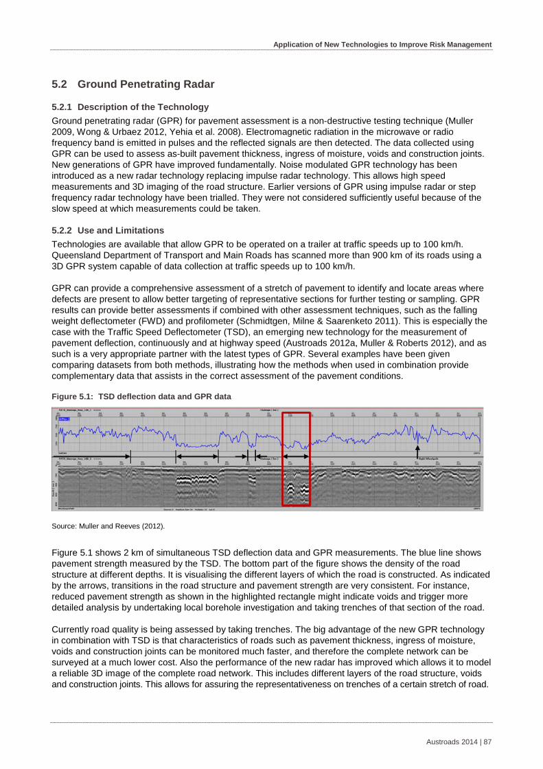
Application of New Technologies to Improve Risk Management
5.2 Ground Penetrating Radar
Description of the Technology 5.2.1Ground penetrating radar (GPR) for pavement assessment is a non-destructive testing technique (Muller 2009, Wong & Urbaez 2012, Yehia et al. 2008). Electromagnetic radiation in the microwave or radio frequency band is emitted in pulses and the reflected signals are then detected. The data collected using GPR can be used to assess as-built pavement thickness, ingress of moisture, voids and construction joints. New generations of GPR have improved fundamentally. Noise modulated GPR technology has been introduced as a new radar technology replacing impulse radar technology. This allows high speed measurements and 3D imaging of the road structure. Earlier versions of GPR using impulse radar or step frequency radar technology have been trialled. They were not considered sufficiently useful because of the slow speed at which measurements could be taken.
Use and Limitations 5.2.2Technologies are available that allow GPR to be operated on a trailer at traffic speeds up to 100 km/h. Queensland Department of Transport and Main Roads has scanned more than 900 km of its roads using a 3D GPR system capable of data collection at traffic speeds up to 100 km/h.
GPR can provide a comprehensive assessment of a stretch of pavement to identify and locate areas where defects are present to allow better targeting of representative sections for further testing or sampling. GPR results can provide better assessments if combined with other assessment techniques, such as the falling weight deflectometer (FWD) and profilometer (Schmidtgen, Milne & Saarenketo 2011). This is especially the case with the Traffic Speed Deflectometer (TSD), an emerging new technology for the measurement of pavement deflection, continuously and at highway speed (Austroads 2012a, Muller & Roberts 2012), and as such is a very appropriate partner with the latest types of GPR. Several examples have been given comparing datasets from both methods, illustrating how the methods when used in combination provide complementary data that assists in the correct assessment of the pavement conditions.
Figure 5.1: TSD deflection data and GPR data
Source: Muller and Reeves (2012).
Figure 5.1 shows 2 km of simultaneous TSD deflection data and GPR measurements. The blue line shows pavement strength measured by the TSD. The bottom part of the figure shows the density of the road structure at different depths. It is visualising the different layers of which the road is constructed. As indicated by the arrows, transitions in the road structure and pavement strength are very consistent. For instance, reduced pavement strength as shown in the highlighted rectangle might indicate voids and trigger more detailed analysis by undertaking local borehole investigation and taking trenches of that section of the road.
Currently road quality is being assessed by taking trenches. The big advantage of the new GPR technology in combination with TSD is that characteristics of roads such as pavement thickness, ingress of moisture, voids and construction joints can be monitored much faster, and therefore the complete network can be surveyed at a much lower cost. Also the performance of the new radar has improved which allows it to model a reliable 3D image of the complete road network. This includes different layers of the road structure, voids and construction joints. This allows for assuring the representativeness on trenches of a certain stretch of road.
Austroads 2014 | 87

Application of New Technologies to Improve Risk Management
Other uses of the new noise modulated GPR are measurements of the depth of the hard shoulder. This information is needed for hard shoulder running and is often not available in records. Also, because the radar is good in detecting water, it can be used to assess when it is safe to reopen roads after flooding. Road agencies currently do not have sufficient data on which to base their decision.
Case Examples 5.2.3A network-level trial with the new Australian made 3-dimensional Noise Modulated Ground Penetrating Radar (NM-GPR) was undertaken in 2010 by the Queensland Department of Transport and Main Roads in which more than 900 lane-kilometres of data were assessed, Muller (2012). Subsequent analysis compared output from the NM-GPR highway speed road measurement with the Danish Traffic Speed Deflectometer (TSD). The examples given in Muller and Reeves (2012) illustrate how these methods can be combined to enable much more rapid and comprehensive investigations of road pavements than is currently possible. Overall the combination of TSD and the new form of 3D NM–GPR methods were found to be complementary, providing significant benefits.
5.3 Origin-destination Data Collection and Travel Time Estimation
Description of the Technology 5.3.1Origin-destination (OD) studies and travel time prediction can be done automatically with technologies such as Bluetooth-based systems and automatic number plate recognition (ANPR) based technologies.
Both of these technologies operate with the same principle of detection of location and time of unique devices or identifiers to estimate OD patterns and journey times, Barcelo et al. (2010), Bodger, Saville and Siddall (2008), Friedrich et al. (2008), Greene (2008), Herrera et al. (2009), Friedrich, Jehlicka and Schlaich (2008), Otterson (2009), Wunnava et al. (2007). SCATS-based systems can also be used to estimate journey times. They are not suitable for OD data collection (Luk et al. 2006).
Another source of origin-destination data and travel time data is the so called floating car data (FCD), which regularly registers speed and location within the car, Van de Weijer (2012). This is usually done using GPS technology. Most navigation systems collect floating car data. Another technology used to generate floating car data uses the strength of the 3G cellular phone network antennas. Both GPS and 3G antenna strength are used in smart phones and are also referred to as phone tracking technologies. These emerging technologies are also currently being described in the update of the Austroads Guide to Traffic Management – Part 3 in the ongoing project NP1695 Guide to Traffic Management – Part 3 update.
Table 5.1 shows a distinctive characteristic of the technologies for OD and travel time estimation. Some technologies monitor vehicles over a fixed trajectory using sensors on the side of the road. Other technologies use sensors in the vehicle. This allows for data collection wherever the vehicle goes. This also means OD data can be collected from the actual origin to the actual destination.
Table 5.1: OD and travel time estimation technologies' characteristics
OD and travel time estimation technology FCD/trajectory based
Bluetooth Trajectory based
ANPR cameras Trajectory based
Cellular antenna FCD
GPS FCD
Austroads 2014 | 88

Application of New Technologies to Improve Risk Management
Use and Limitations 5.3.2Online methods to collect OD and journey time data are reliable and can reduce the overall cost of data collection, which is traditionally done by interview surveys.
The collected OD information and travel time data also allow for new applications. Real-time measurements can be combined with historical data to make more accurate short term and long term predictions for both OD matrices and travel times.
Currently travel times are already widely provided to road users on variable message signs as a route advice. This leads to a better distribution of traffic over the network. Improved OD data and real-time travel time can be used in traffic simulation modelling to support traffic managers in real-time. Different traffic management measures can be simulated based on the real-time data, supporting the traffic manager in implementing the best suitable measures for that situation.
Case Examples 5.3.3Case examples of OD and travel time data collection are as follows:
A pilot was undertaken in Barcelona in 2010 to explore the quality of the data produced by the Bluetooth detection of mobile devices in vehicles for travel time forecasting and to estimate origin-destination matrices on motorways (Barcelo et al. 2010). Bluetooth based vehicle detection proved to be a mature technology that provides sound measurements of average speeds and travel times between sensor locations. The paper proposes an approach to estimate dynamic origin-destination matrices. The approach performs well in uncongested conditions but further research is suggested on how to deal with congested situations.
An Australian case example is the use of Bluetooth on a main arterial route in Brisbane. Travel time obtained from Bluetooth recorded bi-modal travel time in a particular link and captured traffic characteristics in urban arterial streets, such as morning and evening peaks during weekdays, Tsubota et al. (2011). Kieu et al. (2012) compared Bluetooth data from a different route in Brisbane to bus travel times. The travel time estimation models revealed that the not-in-service bus travel time were similar to the car travel times and the in-service bus travel times could be used to estimate car travel times during off-peak hours.
5.4 Smart Work Zone
Description of the Technology 5.4.1A smart work zone is a road construction zone that utilises various electronic devices to inform motorists of the traffic conditions at the work zone and to provide advance information and advice (Bushman & Berthelot 2005, Tudor, Meadors & Plant 2003). A smart work zone typically includes variable message signs, traffic sensors, and software. Traffic sensors at various locations gather traffic speed and queue data and use them to determine the appropriate message to display on the VMS. The messages could include:
advice on re-routing due to long delays
advice on the appropriate speed to take
estimated duration of delays
presence of stopped vehicles.
Messages are determined automatically based on prevailing traffic conditions. Messages can be either in text or in graphics.
Figure 5.2 shows some of the components used in a smart work zone in Springfield Illinois. On the right is the traffic sensor, which is a mobile camera on solar power, and in the background the dynamic message sign is shown.
Austroads 2014 | 89

Application of New Technologies to Improve Risk Management
Figure 5.2: Some of the smart work zone system components
Source: FHWA (2004).
Use and Limitations 5.4.2Smart work zones could improve the route choice decisions of motorists by providing up-to-date traffic condition information. They also have potential benefits to safety by alerting motorists of the presence of stopped vehicles and speed advisories/enforcement (Bushman & Berthelot 2005, Fontaine 2003).
Practical applications of dynamic warning signs that dependent on real-time traffic and roadwork activities in Australia have not been found by this study. The Austroads (2012b) report on Implementing National Best Practice for Traffic Control at Worksites does not mention smart work zones. Changeable message signs are currently being used, however not controlled by the real-time traffic situation and roadwork activities. Australian pilots would be needed to assess the effectiveness of smart work zone technology and further improve traffic efficiency and safety at Australian work zones.
Case Examples 5.4.3Case examples of smart work zones are:
The Arkansas State Highway and Transportation Department (USA) managed two smart work zones on motorways (Tudor, Meadors & Plant 2003). The smart work zones were implemented to improve safety and showed messages such as ‘Slow traffic ahead – be prepared to stop’ and ‘Five mile backup ahead – be prepared to stop’. Based on crash rate analysis it concluded that safety was positively affected.
A smart work zone was implemented on a two-lane highway located about 6 miles north of Manhattan. Based on the speed data analysis results, it was concluded that the graphic-aided and graphic portable changeable message signs were effective in reducing vehicle speeds in the upstream of the one lane two-way work zone, Bai et al. (2011).
In a third example, CCTV cameras were linked with ANPR to monitor and enforce traffic regulations in work zones. Overall, the reaction of local residents to the efforts of North Carolina Department of Transportation was highly positive with more than 95% supporting future projects of this type (McConnell 2010).
The US Federal Highway Administration (2008) did a comparative analysis on the benefits of using ITS in work zones based on data from sites in the District of Columbia, Texas, Michigan, Arkansas, and North Carolina. Quantitative benefits were found for several sites, such as reductions in aggressive manoeuvres at work zone lane drops (Michigan), significant traffic diversion rates and lower observed mainline volumes (Texas, District of Columbia) and the improved ability to react to stopped or slow traffic (Arkansas).
Austroads 2014 | 90

Application of New Technologies to Improve Risk Management
5.5 Roadwork Scheduling Software
Description of the Technology 5.5.1A computer algorithm has been developed by Tang and Chien (2009) to generate roadwork schedules that minimise the total cost to all stakeholders. The costing model takes three components into consideration:
the material, equipment and labour required for each combination of crew size and work time
the risk of works being delayed or suspended due to work times encroaching on peak traffic time periods
road-user costs, which include the cost of increased travel times for motorists, increased vehicle fuel and operation costs, and potential accident costs.
In the UK the impact of pavement maintenance operations on travel time has been assessed. The current UK approach for assessing road maintenance is the Highways Agency Pavement Management System (HAPMS). It includes a module to evaluate the whole-life costs of different pavement maintenance options, known as SWEEP (Software for the Whole-life Economic Evaluation of Pavements). The SWEEP model adopts current parameter values to assess the impact of works in terms of the costs of delays to road users under different traffic management arrangements at maintenance sites, Transport Scotland (2012).
The Transport Research Laboratory (TRL) in the United Kingdom, working for the Highways Agency, has adapted an existing model, the Scheme Analysis System (SAS) to allow its use in different countries. The SAS model is used to analyse treatment options for maintenance schemes on the trunk road network in England and to identify the options that provide good value for money in whole-life cost terms. Based on an Excel spreadsheet, this road project evaluation model allows the user to compare options for different maintenance regimes. TRL developed a variation of the SAS model to make it more suitable for international use, called the PASI model. In the PASI model, various currencies can be represented and users may use their own descriptive terms and apply their own cost and output rates for maintenance treatments and traffic management options. The model includes the capability to make allowances for user costs based on delay times, for residual value and for different treatments on different lanes of the highway. It is also suitable for both concrete and bituminous pavements, OECD (2005).
Use and Limitations 5.5.2Scheduling roadwork is often a complex activity with many different factors to take into consideration. Software that can optimise roadwork scheduling could find a suitable, if not optimal, solution to improve the decision-making process on the co-ordination of roadwork.
Case Example 5.5.3The HAPMS in combination with the SWEEP module was used for a study of a Scottish trunk road network. QUeues And Delays at ROadworks (QUADRO) is a UK Department for Transport (Department for Transport 2002) sponsored computer program which was used to estimate the effects of roadwork in terms of time, vehicle operating and accident costs on the users of the road. Individual roadwork can be combined to produce the total cost of maintaining the road over time. The results of the analysis showed the reductions in pavement budgets would lead to reductions in the amount of work and hence less disruption to traffic on the network. The annual variation in delay costs as the number of notional schemes on each road type changed over the analysis period, Transport Scotland (2012).
Austroads 2014 | 91

Application of New Technologies to Improve Risk Management
6. Discussion and Conclusions
This chapter compares and discusses the new technologies that were rated as the most promising new technologies for use in asset management in Stage 1 of this project.
First this chapter summarises the main findings. Then the technologies are discussed in terms of four main criteria for improving efficiency in asset management which have been addressed in this report. Finally conclusions are drawn about how the potential benefits of these new technologies can be realised.
6.1 Findings This section summarises the main findings for each of the new technologies in this paper.
3D Imaging 6.1.13D imaging (priority 1) has many possible applications in different areas of asset management including safety, infrastructure maintenance planning, and road design, and even in other sectors such as energy.
The benefits of 3D imaging are generally quantified in terms of cost savings in the data collection process. A combined data collection effort between different departments of a road management agency can have a large contribution to a positive business case for their common benefit.
A current limitation to cost-effective use of 3D imaging technologies is that the extraction of relevant features like bridge heights can only partly be automated. Although the distance measurements are automated, the systems cannot always identify the feature they are measuring. The need for manual identification and extraction of measured features such as bridge heights, traffic signs or clear zones can be labour intensive, and therefore automatic extraction is crucial to realising the benefit of 3D imaging.
Wireless Sensor Networks 6.1.2Wireless sensor networks (priority 1) are networks of smart sensors with embedded microprocessors and wireless communication links have the potential to fundamentally change the way in which Australia’s bridges, highways and buildings are monitored, controlled, and maintained.
While the opportunities offered by smart sensing for structural health monitoring are substantial, a number of critical issues need to be addressed before this potential can be realised. Although the smart wireless sensor technology has been rapidly improving, there still remain limitations in hardware, software, and energy supply technology.
Costs of wireless sensor networks are generally much lower than the costs of traditional wired solutions and there are additional benefits in the ability to monitor structures permanently in a way that is non-disruptive to traffic and non-invasive.
Databases and Planning Software 6.1.3Databases and planning software (priority 1) are commonly used in asset management. However, as new data collection technologies are becoming more affordable, automated and practically applicable, large amounts of new data, called ‘Big Data’ are becoming available for asset management applications. However, many databases and planning software cannot accommodate and use this new data and information. Current standards for the specification and cross-referencing of data between parallel areas of application are often lacking. In addition, current data storage and access systems have limitations which may be exceeded by the requirements of Big Data, and the capabilities of software to transform such data into useful information are largely untapped. Databases and planning software play an important role in several aspects asset management. For these reasons the development of databases and planning software to accommodate and use Big Data is expected to have a large impact on asset management processes and decisions.
Austroads 2014 | 92

Application of New Technologies to Improve Risk Management
The scope and complexity of databases and planning software used in asset management vary strongly between road agencies. As do the costs of databases and planning software and the potential benefits of updating and improving them. The costs and benefits of investments in databases are to be determined on a case-by-case basis.
Non-destructive Evaluation Technologies for Structures 6.1.4There is a large range of methods used for non-destructive evaluation of structures (priority 2), using different technologies. These methods are used to assess the conditions and wear and tear of structures as a result of heavy loads, weather or age.
New methods that have been discussed are ground penetrating radar (GPR), infrared thermography, nuclear methods, acoustic or ultrasonic methods, fibre-optic sensors, scour monitoring methods and photogrammetry.
There are two principal ways to look at structures. The first is to assess the structural capacity, which applies to the structure as a whole. The second is to ‘look’ into a structure to determine the internal as-constructed configuration, detect internal defects or determine material properties. This generally tells something about specific parts of the structure. Some methods are suitable for structural capacity assessment; others are more suitable for detecting specific defects.
Another categorisation of the technologies is that some technologies are suitable for continuous monitoring, whilst others are suitable for one-off or periodic assessments.
A growing trend in recent times has been to combine a number of NDE methods for structure investigations. As each NDE method has advantages and limitations; combining disparate methods can provide a cross-check of results which in turn can reduce ambiguity and increase confidence in the interpretations.
Automatic Detection of Overweight Vehicles 6.1.5Automatic detection of overweight vehicles (priority 2) is a combination of weigh-in-motion (WIM) technology and automatic number plate recognition (ANPR) technology, the former to discreetly detect a vehicle and quantify its weight, and the latter to link that evaluation to a particular vehicle. The combination of WIM and ANPR is used at specific locations to protect bridges and sections of highways from damage caused by overweight vehicles and to improve road safety. It is generally used for real-time pre-selection of overweight vehicles for enforcement.
On-board Mass Monitoring 6.1.6On-board mass monitoring (OBM, priority 2) is the measuring of a vehicle’s mass using on-board instrumentation. For trucks, this is achieved through sensors which measure the mass over each axle. These sensors can either be load cells, which measure mass based on the load applied to a strain gauge within the load cell, or air pressure transducers, which measure mass based on the air pressure within an axle’s airbag suspension.
OBM can, for example, be used for heavy vehicle road pricing and for enforcement of heavy vehicle road access. It could also potentially be used to identify and locate road deterioration when linked to a location-based telematics system. Currently there are no standards in place for OBM systems. However, Transport Certification Australia (TCA) is currently developing a type-approval process for assessing OBM units against a nationally-agreed performance-based functional and technical specification. This soon to be available type-approval process should provide transport operators with greater confidence in their use of OBM systems.
Austroads 2014 | 93
Application of New Technologies to Improve Risk Management
Findings on Level 3 Priority Technologies 6.1.7This section describes the findings on the level 3 priority technologies, being Slope monitoring technology, Ground penetrating radar, Origin-destination data collection, Smart work zone and Roadwork scheduling software. It addressed their potential use in asset management.
The depth and scope of the assessment of level 3 priority technologies was limited to a one page description of each technology addressing the concept of the technology, the possible use in asset management and its limitations, and case examples. Based on the case examples and the potential use in Australian asset management practice, the following is concluded:
Radar based slope monitoring technology is a technology that is in the initial development phase for road applications. It has been applied in open cut mines and would still need to be piloted and possibly adapted for road safety purposes. A logical next step would be to undertake technical field tests.
A promising new technological development from the classical asset management perspective that is implemented in a market ready solution and is extensively tested is the noise modulated ground penetrating radar (GPR). A next step is a broad Australia-wide deployment.
Origin-destination (OD) data collection and travel time data collection techniques are technologies that are fully operational. These technologies are traditionally used for traffic management application, so the use of these technologies in the context of asset management is new. Next steps could focus on the integration with asset management processes. Origin-destination data can for example be used for demand prediction when planning investments in road maintenance.
Smart work zones are another technology that is currently used for traffic management. The smart work zones contribute to a safer maintenance of roads with fewer disturbances for traffic. Although smart work zones are already being used, next steps are to further improve safety by making smart work zones more traffic and work dependent, and to extend and personalise the communication channels to e.g. road agency websites, apps and in-car navigation.
Scheduling roadwork is often a complex activity with many different factors to take into consideration. Software that can optimise roadwork scheduling could find a suitable, if not optimal, solution to improve the decision-making process on the co-ordination of roadwork. A possible next step is to assess the potential savings using the new algorithms described in this document.
6.2 Discussion This section discusses the new technologies in terms of four main criteria for improving efficiency in asset management which have been addressed in this report. These criteria are:
potential use in asset management
market readiness and current limitations related to that
quality of the data (i.e. scope, accuracy, detail, and repeatability)
costs and business case issues.
These criteria were used in Stage 1 of the project to prioritise a long list of new technologies.
Potential Use in Asset Management 6.2.1The new technologies assessed in this report can be applied to different areas of asset management. Some technologies have a very specific use, while others have a much broader use, and therefore potentially a larger impact.
Where 3D imaging technology (e.g. LiDAR) can be applied to a range of areas including safety, infrastructure maintenance planning and road design, wireless sensor networks are applicable to the specific area of structural health monitoring. Databases and planning software and the use of Big Data can also be applied across all areas of asset management. Therefore, the potential impact of 3D imaging and better use of Big Data by databases and planning software is expected to be larger than that of wireless sensor networks.
Austroads 2014 | 94
Application of New Technologies to Improve Risk Management
Non-destructive evaluation technologies are used for the assessment of the conditions and wear and tear of structures as a result of heavy loads, weather or age. Automatic detection of overweight vehicles can be used to protect structures and roads from excessive wear by identifying overweight vehicles to warn them or select them for official weighing. On-board mass monitoring could be used for access control, mass-based road pricing or to identify and locate road deterioration. A combination of these three new technologies can be applied to assess the risk of deterioration of roads and structures and to manage the loads on the network by allowing access of heavy vehicles based on their actual accurate weight. On-board mass monitoring has potentially the largest impact on asset management of these three technologies as it could provide accurate weight data throughout the network which allows for both more refined access management and assessment of the impact.
Market Readiness and Current Limitations 6.2.2Some technologies are more ‘new’ than others. The development stage of the technologies ranges from those that still need to be tested on the road for the first time to technologies that are fully operational and matured in other parts of the world.
LiDAR, the most common 3D imaging technology, is being used increasingly, for example in the USA but also in Australia. Although LiDAR has been developing quickly, and continues to do so, it is ‘market ready’, much more so than for example wireless sensor networks or applications of Big Data in asset management databases and planning software. Wireless sensor networks are currently being piloted. For specific cases like the Sydney Harbour Bridge, the technology already has huge benefits. For more standardised applications, the technology needs further development.
Non-destructive evaluation technologies for structures are being used to assess the damage to structures when issues are evident. However they are being used more frequently and increasingly for monitoring purposes. There is a range of methods in different stages of maturity. Most innovations are incremental improvements of existing systems.
Automatic detection of overweight vehicles is a combination of two very mature technologies, weigh-in-motion and automatic number plate recognition. The combination of both technologies has been deployed numerous times as well. First generations of on-board mass monitoring systems are commercially available as both aftermarket and built-in systems. Type approval procedures are currently being developed in Australia.
Quality of the Data 6.2.3The quality of the data can be expressed in terms of e.g. scope, accuracy, detail, and repeatability. Both 3D imaging (e.g. LiDAR) and wireless sensor networks provide high quality data. These technologies score high on scope, accuracy, detail as well as repeatability. For both technologies the challenge is in extracting the useful information. Database and planning software uses existing data. The quality of the information produced by these systems depends on the quality of the data that is used as an input. Current data sets are sometimes incomplete and partly out-of-date.
Several of the technologies in this report address the risk of deterioration of roads and bridges by heavy or overweight vehicles. The type and quality of the data collected by these technologies are very different. Non-destructive evaluation technologies often collect very specific data (small scope) in high detail and with high accuracy. Systems for automatic detection of heavy vehicles collect data for all passing vehicles; however, the accuracy is insufficient for legal weighing. On-board mass monitoring provides similar accuracies in terms of weight; however, the scope is very different. Rather than collecting data for every vehicle in a specific location, it collects data for specific vehicles throughout the network.
Austroads 2014 | 95
Application of New Technologies to Improve Risk Management
Costs and Business Case 6.2.4Indicative cost figures have been identified for the new technologies addressed in this report. Additionally statements about the business case and the most relevant cost components and benefits have been included when available.
A benefit of 3D imaging is the wide range of possible applications. The business case for 3D imaging is often not positive when looking at one application at the time. However, a number of case studies have shown than collecting 3D images once and (re)use them for a range of applications does results in a positive business. This will require coordination between different departments within road agencies. 3D imaging is ‘market ready’, has a large number of potential uses and has been shown to have a positive business case in several case studies. It is considered the most promising new technology for asset management.
The benefits for the accommodation of Big Data in asset management databases and planning software are hard to predict and require more research in specific applications. The large number of impact areas for the use of Big Data and the fast developments in this area make this a very promising ‘new technology’ as well.
As wireless sensor networks are applied in clearly scoped projects like monitoring a bridge, it has a clear business case. The business case for wireless sensor networks is potentially very good due to the possible reduction in labour for installation and the decreasing prices for the sensor technology.
The costs for applying non-destructive evaluation (NDE) technologies vary for the different technologies. Even more so, these technologies are constantly evolving, so the associated cost and complexity involved are being improved. The costs of systems that automatically detect overweight vehicles depend on the type of system and the desired accuracy. The benefits can be expressed in terms of more efficient use of weighing stations and enforcement personnel, and in benefits for the industry as vehicles do not need to stop when they comply with weight restrictions.
The total costs for on-board mass monitoring systems vary between $5000 and $17 000 per vehicle, depending on the type of system and the type of vehicle. The business case is still unclear as the benefits and the distribution of the benefits over the road agencies and the operators depend on how the system will be implemented in the fleet. For legislative applications there will be costs involved to ensure compliance with the legal requirements for the on-board devices. This is yet to be determined.
6.3 Conclusions The following suggestions are made to guide road agencies in the adoption of these new technologies. These suggestions are based on the findings from the literature review and the stakeholder consultations.
3D Imaging 6.3.1Because of the potential of 3D imaging of roads and roadsides it is likely to get a prominent place in different areas of asset management. To realise the potential and overcome the current difficulties of extracting information from point clouds in an automated and efficient manner, a common platform to exchange best practice in feature extraction and the development of national standards for mobile 3D imaging surveys could be initiated.
Wireless Sensor Networks 6.3.2Wireless sensor networks have a large potential in structural health monitoring. Since wireless sensor networks are still in a piloting stage and have technical limitations, road agencies could engage with knowledge institutes and to facilitate pilots that can contribute to overcoming the current limitation of wireless sensors and encourage the development of smart new algorithms to determine structural health indicators based on wireless sensor networks.
Austroads 2014 | 96

Application of New Technologies to Improve Risk Management
Database and Planning Software 6.3.3Database and planning software has not kept up with the Big Data that has become available due to new data collection technologies such as 3D imaging, wireless sensor networks, laser crack measurement systems, traffic speed deflectometers and others. Therefore it is suggested to further develop databases and planning software used in asset management for the accommodation of Big Data, in terms of standards, storage and access, with the consequential flow-on to improvements in the application of Big Data as input to planning software. A possible next step is the assessment of the scalability of current databases and planning software systems for the fruitful exploitation of Big Data. The purpose of such an exercise would be to define recommendations for the reorganisation of asset management information systems, the solution to questions seeking the added value of new data collection technologies, and discovering how current data management systems could best accommodate, process and manage the Big Data emanating from such new technologies.
Non-destructive Evaluation Technologies for Structures 6.3.4Non-destructive evaluation (NDE) technologies are to be used when there is a risk that the structural capacity of a bridge or another structure is deteriorating. This could be due to frequent use by heavy vehicles, flooding or old age. There is a range of NDE technologies with different strengths and weaknesses. When considering the assessment of a structure the appropriate technology, or combination of technologies, should be determined to address the specific risk. If the purpose of an assessment of a bridge that faces frequent use by heavy vehicles is to determine the deterioration rate and predict required maintenance, it might benefit from continuous monitoring rather than a one-off assessment.
Automatic Detection of Overweight Vehicles 6.3.5The accuracy of weigh-in-motion (WIM) systems is insufficient for enforcement purposes. WIM systems for automatic detection of overweight vehicles are mainly usable in situations where static roadside weigh stations are not feasible (e.g. because of space limitations), or to improve the efficiency of roadside static weigh stations by preselecting vehicles that are likely to be overweight.
On-board Mass Monitoring 6.3.6On-board mass monitoring (OBM) has the potential to efficiently collect valuable data on vehicle weight throughout the network and the impact of overweight vehicles on roads and structures such as bridges. Most heavy vehicles, both prime movers and trailers, are already equipped with sensors that could be used for OBM. A possible way to realise the potential of this technology is to use OBM as part of a mass-distance or mass-distance-location based road pricing scheme. As the damage to roads and structures is exponential to the weight of the vehicle, the risk of damage applies to vehicles above a certain weight. In the context of the Heavy Vehicle Charging and Investment Reform in Australia a mass-based pricing system is considered. In this context on-board mass monitoring could be deployed in vehicles above a certain weight. This can kick-start the deployment of telematics devices which can make the data, collected by the vehicle sensors, available outside the vehicle for asset management purposes.
Conclusions on Level 3 Priority Technologies 6.3.7This section provides conclusions on the level 3 priority technologies, being Slope monitoring technology, Ground penetrating radar (GPR), Origin-destination (OD) data collection, Smart work zones and Roadwork scheduling software.
The depth and scope of the assessment of level 3 priority technologies was limited to a one page description of each technology addressing the concept of the technology, the possible use in asset management and its limitations, and case examples. Based on the case examples and the potential use in Australian asset management practice, the following is concluded on how to realise the potential benefits of each of these technologies for asset management:
To realise the potential benefits of Slope monitoring technology it is suggested to test the technologies that are currently applied in open cut mines during road construction and reconstruction projects on slopes for which a risk of slides is identified.
Ground penetrating radar technology can now be applied at travel speed. To realise the potential benefits it is suggested to include travel speed GPR measurements to road condition surveys.
Austroads 2014 | 97

Application of New Technologies to Improve Risk Management
High quality origin-destination data is quickly becoming available from GPS based probe data from
connected vehicles and smartphones, also called Origin-destination data collection technologies. It is suggested to use origin-destination data for predicting travel demand when planning investments for road infrastructure (re)development.
It is suggested to further improve safety at work zones by making existing Smart work zones more intelligent and situation dependent.
Scheduling roadwork is often a complex activity with many different factors taken into consideration. To optimise societal benefits it is suggested to consider and test new algorithms for Roadwork scheduling software which include the significant cost component of road user costs, including the risk of work being delayed into peak traffic periods.
6.4 Links to Austroads Guides To consolidate the content of this report, it is suggested that it be incorporated into the suite of Austroads Guides, as these are the main reference for good practice used by road agencies.
The suggested place to include (a summary of) this content is the Guide to Asset Management – Part 5A: Inventory, which addresses data collection and processing of asset inventory and conditions. This can be included in Section 6 Data Collection Methods and Section 7 Data Processing, or in a new section on New Technologies. It is suggested to include at least a summary description of the technologies and the findings and conclusions, and a reference to the current report for more details.
Additionally, cross-references in other guides are suggested in Table 6.1.
Table 6.1: Suggested cross references to Austroads Guides
Technologies Austroads Guides to cross reference AT1539 content
Top priority technologies
3D imaging GAM – Part 5A: Inventory and national standard/guideline for mobile LiDAR
DBPS GAM – Part 5A: Inventory and GAM – Part 3: Asset Strategies
Wireless sensor networks GAM – Part 6: Bridge Performance
Level 2 priority technologies
Detection of overweight vehicles GTM – Part 4: Network Management and GAM – Part 3: Asset Strategies
On-board mass monitoring GTM – Part 4: Network Management and GAM – Part 3: Asset Strategies
NDE technologies for structures GAM – Part 6: Bridge Performance
Level 3 priority technologies
Slope monitoring technology GRS – Part 9: Roadside Hazard Management
GRP for pavement assessment GAM – Part 5D: Pavement Performance – Strength
O-D and travel time data collection GTM – Part 4: Network Management
Smart work zone GTM – Part 9: Traffic Operations
Roadwork scheduling software GAM – Part 4: Program Development and Implementation
GAM = Guide to Asset Management, GTM = Guide to Traffic Management, GRS = Guide to Road Safety.
Austroads 2014 | 98
Application of New Technologies to Improve Risk Management
References
3D Laser Mapping n.d., StreetMapper bridges the highways survey gap, web article, viewed 13 November 2012, http://www.3dlasermapping.com/index.php/news-events/news-stories/163-streetmapper-bridges-the-highways-survey-gap.
Accuweigh 2013a, Loadcells - Vishay PM Onboard, webpage, Accuweigh, Melbourne, Vic, viewed 1 October 2013, <http://www.accuweigh.com.au/Products/Loadcells-Vishay-PM-Onboard-170.aspx>.
Accuweigh 2013b, PM1200 indicator Bluetooth feature, webpage, Accuweigh, Melbourne, Vic, viewed 1 October 2013, <http://www.accuweigh.com.au/Uploads/Resources/Folder0/PM1200D-Onboard-Digital-Indicator-with-Bluetooth-Brochure-1118.pdf>.
Alves, M 2009, The WSN standards and COTS landscape: can we get QoS and ‘calm technology’?, presentation, CONET Cooperating Objects NETwork of Excellence consortium, 7th Framework Programme, EU.
American Concrete Institute 1998, Non-destructive test methods for evaluation of concrete in structures, report ACI 228.2R-98, ACI, Farmington Hills, MI, USA.
Arcadis 2009, Advanced inspections project: innovative technologies to improve highway condition monitoring, report no. D03031.001999, Dutch Ministry for Infrastructure and Environment, Netherlands.
ASTM 2009, Standard specification for highway weigh-in-motion (WIM) systems with user requirements and test methods, E1318-09, American Society for Testing Materials, West Conshohocken, PA, USA.
AusRAP 2006, Star ratings: Australia’s national network of roads, Australian Automobile Association, Canberra, ACT.
Australian Local Government Association & ANZLIC 2007, ‘Data management principles’ in Local government spatial information management toolkit, version 2.0, ALGA, Canberra, ACT, module 3, pp. 93-116.
Austroads 2000, Weigh-in-motion technology, AP-R168-00, Austroads, Sydney, NSW.
Austroads 2010, Weigh-in-motion management and operation manual, AP-T171-10, Austroads, Sydney, NSW.
Austroads 2011, Feasibility study: heavy vehicle charging in Australia, AP-R384-11, Austroads, Sydney, NSW.
Austroads 2012a, Application of new technologies to improve risk management (stage 1): scoping of potential technologies, AP-T205-12, Austroads, Sydney, NSW.
Austroads 2012b, Implementing national best practice for traffic control at worksites: risk management, audit and field operations, AP-R403-12, Austroads, Sydney, NSW.
Bai, Y, Huang, Y, Schrock, S, Li, Y 2011, Determining the effectiveness of graphic-aided dynamic message signs in work zone, The University of Kansas, Kansas, USA, viewed 22 October 2012, <http://www.intrans.iastate.edu/smartwz/documents/project_reports/BaiGraphicAidedDMSFinal%20Report.pdf>.
Barcelo, J, Montero, L, Marques, L & Carmona, C 2010, ‘Travel time forecasting and dynamic origin–destination estimation for freeways based on Bluetooth traffic monitoring’, Transportation Research Record, no. 2175, pp.19–27.
Bentley Systems 2010, Point clouds in MicroStation V8i, presentation, Bentley Systems, Melbourne, Vic, viewed April 2013, <http://ftp2.bentley.com/dist/collateral/docs/microstation/MicroStation_and_Point_Clouds.pdf>.
Bodger, M, Saville, L & Siddall, T 2008, ‘The practical application of ANPR for journey time monitoring in Essex’, Traffic Engineering and Control, vol. 49, no. 7, pp.258-60.
Austroads 2014 | 99

Application of New Technologies to Improve Risk Management
Boulis, A, Berriman, R, Attar, S & Tselishchev, Y 2011, ‘A wireless sensor network test–bed for structural
health monitoring of bridges’, IEEE international workshop on practical issues in building sensor network applications, 6th, 2011, Bonn, Germany, Institute of Electrical and Electronics Engineers (IEEE), New York, USA, pp. 1019–22, viewed 30 January 2012, <http://www.nicta.com.au/pub?doc=4908>.
BPW 2013, ECO air compact - the new standard, webpage, BPW, Wiehl, Germany, viewed 1 October 2013, <http://www.bpw.de/fileadmin/data/downloads/BPW-ECO_Air_COMPACT_15191202e.pdf>.
Bungey, JH, Millard, SG & Grantham, MG 2006, Testing of concrete in structures, 4th edn, Taylor & Francis, Oxford, UK.
Bushman, R & Berthelot, C 2005, ‘Response of North Carolina motorists to a smart work zone system’, Transportation Research Board annual meeting, 2005, Washington, DC, TRB, Washington, DC, USA, paper no. 05–0968, viewed 31 January 2012, <ssom.transportation.org/Documents/05–0968.pdf>.
Carino, NJ 2001, ‘The impact-echo method: an overview’, Structures congress and exposition, 2001, Washington, DC, American Society of Civil Engineers, Reston, Virginia, USA, pp. 1-18.
Cho, S, Yun, C, Lynch J, Zimmerman, A, Spencer, B & Nagayama, T 2008, ‘Smart wireless sensor technology for structural health monitoring of civil structures’, Steel Structures, vol. 8 , no. 4, pp. 267-75.
Choudhury, M & Rizos, C 2010, ‘Slow structural deformation monitoring using Locata: a trial at Tumut Pond dam’, Journal of Applied Geodesy, vol. 4, no. 4, pp.177–87, viewed 30 January 2012, <www.gmat.unsw.edu.au/snap/publications/mazher&rizos2010a.pdf>.
Chung, WH, Liu, SY, Guan, BO, Chan, TL, Chan, THT & Tam, HY 2003, ‘Structural monitoring of Tsing Ma bridge using fiber Bragg grating sensors’, Optoelectronics, 6th, 2003, Chinese symposium, IEEE, pp.144-6.
Constant, M n.d., An Introduction to ANPR, webpage, CCTV Advisory Service, UK, viewed 4 October 2013, <www.cctvinformation.com>.
Cracknell, A & Hayes, L 2007, Introduction to remote sensing, 2nd edn, Taylor and Francis, UK.
CROSS 2013, Weigh-in-motion & traffic counters, web article, CROSS, Czech Republic, viewed 28 January 2014, <http://www.cross.cz/en/references/wim-traffic-counters.html>.
Davis, L & Sack, R 2006, ‘Determining heavy vehicle suspension dynamics using an on-board mass measurement system’, ARRB conference, 22nd, 2006, Canberra, ACT, Australia, ARRB Group, Vermont South, Vic, 19pp.
Department for Transport, UK 2002, ‘QUADRO4 user manual’, Design manual for roads and bridges: volume 14: economic assessment of road maintenance: QUADRO user manual, Department for Transport, London, UK, viewed 22 October 2012, <http://www.dft.gov.uk/publications/quadro-4-manual/ >.
Department of Main Roads 2005, Timber bridge maintenance manual: appendix D: non-destructive testing, Department of Transport and Main Roads, Brisbane, Qld.
Dietsch, P & Köhler, J (eds) 2010, Assessment of timber structures, COST action E55, Shaker, Germany.
Ding, XL, Dai, WJ, Yang, WT, Zhou, XW, Lam, J, Zhang, Q & Wang, L 2007, ‘Application of multi–antenna GPS technology in monitoring stability of slopes’, FIG working week 2007 in Hong Kong, SAR, China, FIG, International Federation of Surveyors, Copenhagen, Denmark, 11pp, viewed 30 January 2012, <http://www.fig.net/pub/fig2007/papers/ts_3f/ts03f_04_ding_etal_1399.pdf>.
EarthMine n.d., Earthmine technology introduction, online video presentation, earthmine Australia, WA, viewed November 2011, <http://www.earthmineaustralia.com/Solutions?Overview>.
Ellsworth, P 2013, ‘Utah DOT leveraging LiDAR for leap to asset management’, LiDAR Magazine, vol. 3, no. 1.
Enckell, M, Glisic, B, Myrvoll, F & Bergstrand, B 2011, ‘Evaluation of a large-scale bridge strain, temperature and crack monitoring with distributed fibre-optic sensors’, Journal of Civil Structural Health Monitoring, vol. 1, no.1-2, pp. 37-46.
Engel, J, Zhao, L, Fan, Z, Chen, J & Liu, C 2004, ‘Smart brick: a low cost, modular wireless sensor for civil structure monitoring’, International conference on computing, communications and control technologies (CCCT 2004), Austin, Texas, USA, University of Texas, Austin, USA.
Austroads 2014 | 100

Application of New Technologies to Improve Risk Management
Farrar, C 2001, Historical overview of structural health monitoring, lecture notes, Los Alamos Dynamics, Los
Alamos, New Mexico, USA.
Fayyad, U, Piatetsky-Shapiro, G & Smyth, P 1996, From data mining to knowledge discovery in databases, American Association for Artificial Intelligence, USA.
Fletcher, E & Theron, A 2011, Performance of open graded porous asphalt in New Zealand, research report 455, NZ Transport Agency, Wellington, NZ.
FHWA 2004, Intelligent transportation systems in work zones: a case study: real-time work zone traffic control system, FHWA-HOP-04-018, Department of Transportation, Federal Highway Administration, Washington, DC, USA, viewed 22 October 2012, <http://www.ops.fhwa.dot.gov/wz/technologies/springfield/index.htm>.
FHWA 2008, Comparative Analysis Report: The Benefits of Using Intelligent Transportation Systems in Work Zones, FHWA-HOP-09-002, Department of Transportation, Federal Highway Administration, Washington, DC, USA, October 2008
Fontaine, MD 2003, ‘Guidelines for application of portable work zone intelligent transportation systems’, Transportation Research Record, no. 1824, pp.15-22.
Frecks, M 2008, ‘Dynamic scanning for KDOT: 6.6 miles of urban interstate in 4 hours’, SPAR 2008: capturing and managing existing-conditions data for design, construction and operations, Houston, Texas, USA, SPAR Point Group, Portland, Maine, USA.
Frecks, MR 2012, StreetMapper bridges the highways survey gap, web page 3D laser mapping, Bingham, Nottingham, UK, viewed 13 November 2012, <http://www.3dlasermapping.com/index.php/news-events/news-stories/163-streetmapper-bridges-the-highways-survey-gap>.
Friedrich, M, Jehlicka, P & Schlaich, J 2008, ‘Automatic number plate recognition for the observance of travel behaviour’, International conference on survey methods in transport, 8th, France, International Steering Committee for Travel Survey Conferences, viewed 20 January 2012, <http://isctsc.let.fr/papiers/workshop%20final%20version/21%20B2%20Friedrich%20et%20al.pdf>.
Gakstatter, E, Murfin, T & Shears, W 2011, ‘Locata: a new constellation’, GPS World, September 2011, viewed 30 January 2012, <http://www.gpsworld.com/survey/locata–a–new–constellation–12031?page_id=1>.
Gao, Y & Spencer, B 2008, Structural health monitoring strategies for smart sensor networks, report series no. 011, Newmark structural engineering laboratory, University of Illinois, Urbana-Champaign, IL, USA.
Garnier, V 2012, ‘Ultrasound through transmission’, in D Breysse (ed), Non-destructive assessment of concrete structures: reliability and limits of single and combined techniques, RILEM State-of-the-Art Reports, vo. 1, Springer, Netherlands.
Glennie, C & Taylor, R 2008, ‘TITAN: kinematic terrestrial LiDAR, results and experiences’, SPAR 2008: capturing and managing existing-conditions data for design, construction and operations, Houston, Texas, USA, SPAR Point Group, Portland, Maine, USA.
Graefe, G 2010, ‘High-end applications for kinematic engineering surveying’, SPAR 2010, SPAR Point Group, Portland, Maine, USA.
Greene, K 2008, ‘Tracking traffic with cell phones’, Technology Review, 11 November 2008, MIT, Cambridge, MA, USA, viewed 30 January 2012, <http://www.technologyreview.com/computing/21658/page1/>.
Gucunski, N, Imani, A, Romero, F, Nazarian, S, Yuan, D, Wiggenhauser, H, Shokouhi, P, Taffe, A & Kutrubes, D 2013, Nondestructive testing to identify concrete bridge deck deterioration, SHRP 2 report S2-R06A-RR-1, Strategic Highway Research Program Transportation Research Board, Washington, DC, USA.
Harries, N 2008, ‘The use of slope stability radar in managing slope instability hazards’, AusIMM Bulletin, Jan/Feb 2008, pp.53–4.
HDM Global 2013, HDM-4 version 2, web article, HDM Global, viewed April 2013, <http://www.hdmglobal.com/>.
Austroads 2014 | 101

Application of New Technologies to Improve Risk Management
Herrera, JC, Work, DB, Herring, R, Ban, X & Bayen, AM 2009, Evaluation of traffic data obtained via GPS–
enabled mobile phones: the mobile century field experiment, report UCB–ITS–VWP–2009–8, Center for Future Urban Transport, University of California Berkeley, Berkeley, CA, USA, viewed 20 December 2011, <http://www.ce.berkeley.edu/~bayen/journals/tr_c09.pdf>.
Huefner Management Systems n.d., Asset management systems, brochure, Huefner Management Systems, Adelaide, SA, viewed 31 January 2012, <http://www.huefner.com.au/Brochures/RoadPAK%20Overview%20A3.pdf>.
Illinois SHM Project n.d, About the Illinois SHM project, project website Illinois SHM Project, Open Systems Laboratory & Smart Structures Technology Laboratory, University of Illinois, Urbana-Champaign, IL, USA, viewed January 2013, <http://shm.cs.uiuc.edu/about.html>.
ITS International 2009, Developing an integrated WIM/ANPR enforcement system, web article, ITS International, viewed October 2013, <http://www.itsinternational.com/categories/enforcement/features/developing-an-integrated-wim-anpr-enforcement-system/>.
Jáuregui, DV, White, KR, Woodward, CB & Leitch, KR 2003, ‘Noncontact photogrammetric measurement of vertical bridge deflection’, ASCE Journal of Bridge Engineering, vol. 8, no. 4, pp. 212-22.
Karl, C & Han, C 2007, ‘Heavy vehicle on-board mass-monitoring: capability review’, contract report, ARRB Group, Vermont South, Vic.
Karlovsek, J, Scheuermann, A, Muller, W &Williams, DJ 2011, ‘Application of ground penetrating radar to testing tunnel integrity’, Australasian tunnelling conference: development of underground space, 14th, Auckland, New Zealand, Australasian Institute of Mining and Metallurgy, pp. 529-41.
Kee, SH, Oh, T, Popovics, JS, Arndt, RW & Zhu, J 2012, ‘Nondestructive bridge deck testing with air-coupled impact-echo and infrared thermography’, Journal of Bridge Engineering, vol. 17, no. 6, pp. 928-39.
Kieu, LM, Bhaskar, A & Chung, A 2012, ‘Bus and car travel time on urban networks: integrating Bluetooth and bus vehicle identification data’, ARRB conference, 25th, 2012, Perth, Western Australia, ARRB Group, Vermont South, Vic, 19pp.
Kim, S, Pakzad, S, Culler, D, Demmel, J, Fenves, G, Glaser, S & Turon, M 2007, Health monitoring of civil infrastructures using wireless sensor networks, University of California, Berkeley, USA, viewed 3 February 2012, <http://www.cs.berkeley.edu/~binetude/work/ipsn07_ggb.pdf>.
Koniditsiotis, C, Buckmaster, R & Fraser, P 1995, ‘Australian high speed weigh-in-motion: an overview’, International symposium on heavy vehicle weights and dimensions, 4th, 1995, Ann Arbor, Michigan, USA, University of Michigan, USA.
Krause, M & Mielentz, F 2012, ‘Ultrasonic echo’, in D Breysse (ed), Non-destructive assessment of concrete structures: reliability and limits of single and combined techniques, RILEM State-of-the-Art Reports, vo. 1, Springer, Netherlands.
Leach, I 2013, ‘WIMPR (Weight In Motion & Automatic Number Plate Recognition): identifying overweight vehicles crossing the Auckland Harbour Bridge’, presentation to the ITS summit 2013: smart transport, September, Sydney, NSW, ITS Australia, Melbourne, Vic.
Loadman 2013, Loadman fifth wheel load cell systems, webpage, Loadman Australia, Prospect, NSW, viewed 1 October 2013, <http://www.loadman.com.au/pdf/Loadman%20Brochure%20Fifth%20Wheel%20Scale%20Systems.pdf>.
Lueker, M, Marr, J, Ellis, C, Winsted, V & Akula, SR 2010, Bridge scour monitoring technologies: development of evaluation and selection protocols for application on river bridges in Minnesota, report MN/RC 2010-14, Minnesota Department of Transportation, Minnesota, USA.
Luk, JYK, Karl, C, Su, M & Bennett, P 2006, ‘Real time estimation of travel times on arterial roads in Melbourne’, ARRB conference, 22nd, 2006, Canberra, Australian Capital Territory, ARRB Group, Vermont South, Vic, 14 pp.
Austroads 2014 | 102
Application of New Technologies to Improve Risk Management
Lynch, J 2004, ‘Overview of wireless sensors for real-time health monitoring of civil structures’, Proceedings
of the 4th International Workshop on Structural Control (IWSC), New York City, USA, DEStech Publications, Lancaster, PA, USA.
Lynch, J & Loh, K 2006, ‘A summary review of wireless sensors and sensor networks for structural health monitoring’, The Shock and Vibration Digest, vol. 38 no. 2, pp. 91-128.
MANDLI n.d. Mobile LiDAR, web page, MANDLI, Madison, WI, USA, viewed 13 November 2012, <http://www.mandli.com/>.
McConnell, D 2010, ‘Improving road worker safety’, International Road Federation world meeting, 16th, 2010, Lisbon, Portugal, International Road Federation, Geneva, Switzerland, no. 166, 5pp.
Minkina, W & Dudzik, S 2009, Infrared thermography: errors and uncertainties, Wiley, UK.
Muller, W 2001, ‘Trial of ground penetrating radar to locate defects within timber girders’, Institute of Public Works Engineers Australia Queensland state conference, Noosa, Queensland, IPEWAQ, Brisbane, Qld, 10 pp.
Muller, W 2003, ‘Timber girder inspection using ground penetrating radar’, Non-Destructive Testing and Condition Monitoring, vol. 45, no. 12, pp. 809-12.
Muller, W 2008, ‘GPR inspection of the world’s longest timber bridge’, Structural faults and repair conference, 12th, Edinburgh, UK, Engineering Technics Press, Edinburgh, UK, 43 pp.
Muller, W 2009, ‘Application of ground penetrating radar to road pavement rehabilitation’, Queensland Roads, no.7, March 2009, pp.17-24, viewed 30 January 2012, <http://www.tmr.qld.gov.au/~/media/57b7aab2–7918–4b18–a528–529fd2b11615/aogprtrpr0903qldroads.pdf>.
Muller, W 2012, ‘A network-level road investigation trial using Australian-made traffic-speed 3D ground penetrating radar (GPR) technology’, ARRB conference, 25th, 2012, Perth, Western Australia, ARRB Group, Vermont South, Vic, 18pp.
Muller, W, Karlovsek, J, Reeves, V, Scheuermann, A, Dux, P & Williams, D 2010, ‘Characterising moisture and other properties of civil engineering infrastructure using GPR’, European conference on moisture measurement, 1st, Aquametry, Weimar, Germany, Bauhaus University, Germany, pp. 441-9.
Muller, W & Roberts, J 2012, ‘Revised approach to assessing Traffic Speed Deflectometer (TSD) data, and field validation of deflection bowl predictions’, International Journal of Pavement Engineering, September 2012, DOI:10.1080/10298436.2012.715646.
Muller, WB & Reeves, BA 2012, ‘Comparing traffic speed deflectometer and noise-modulated ground penetrating radar data for rapid road pavement investigations’, International conference on ground penetrating radar (GPR), 14th, 2012, Shanghai, China, Institute of Electrical and Electronics Engineers, New York, USA.
Nagayama, T, Spencer B, Mechitov, K & Agha, G 2008, ‘Middleware services for structural health monitoring using smart sensors’, Smart Structures and Systems, vol.5, no.2, 31pp.
National Policing Improvement Agency 2009, Practice advice on the management and use of automatic number plate recognition, NPIA, London, UK.
National Policing Improvement Agency 2011, National ACPO ANPR standards (NAAS), version 4.12, NPIA, London, UK.
National Transport Commission 2010a, Draft national in-vehicle telematics strategy: the road freight sector, NTC, Melbourne, Vic.
National Transport Commission 2010b, Heavy vehicle pricing options: development and assessment framework: discussion paper, NTC, Melbourne, Vic.
New Zealand Transport Agency 2010, Freight management strategy, NZTA, Wellington, NZ.
Nobles, A & Ward, D 2009, ‘Mobile mapping validation’, SPAR 2009 conference, Denver, Colorado, SPAR Point Group, Portland, Maine, USA.
OECD 2005, Economic evaluation of long-life pavements: phase 1, Organisation for Economic Co-Operation and Development, Paris, France, viewed 22 October 2012, <http://www.internationaltransportforum.org/pub/pdf/05PavementI.pdf>.
Austroads 2014 | 103

Application of New Technologies to Improve Risk Management
Optech n.d., Lynx Mobile Mapper: summary specification sheet, brochure, Optec, Ontario, Canada, viewed
3 January 2013, <http://www.optech.ca/pdf/Lynx_SpecSheet_110909_web.pdf>.
Otterson, JD 2009, ‘Traffic performance measures for the future using today’s technology’, Australian Institute of Traffic Planning and Management (AITPM) national conference, 2009, Adelaide, South Australia, Australian Institute of Traffic Planning and Management (AITPM), Adelaide, SA, 16 pp.
Pank, W 2011, ‘Auckland harbour bridge box girder strengthening design’, Austroads bridge conference, 8th, 2011, Sydney, New South Wales, Austroads, Sydney, NSW.
PIARC 2012, Inspector accreditation, non-destructive testing and condition assessment for bridges, report 2011R07, PIARC Technical Committee D3 Road Bridges, Paris, France.
Pieraccini, M 2013, ‘Monitoring of civil infrastructures by interferometric radar: a review’, The Scientific World Journal, vol. 2013, article ID 786961, doi:10.1155/2013/786961.
Redstall, M 2006, ‘Accurate terrestrial laser scanning from a moving platform’, Geomatics World, 2006, July-August, pp. 28-30.
Rice, J, Mechitov, K, Spencer, B & Agha, G 2008, A service-oriented architecture for structural health monitoring using smart sensors, World conference on earthquake engineering, 14th, Beijing, China, International Association for Earthquake Engineering (IAEE).
Riggio, M, Anthony, RW, Augelli, F, Kasal, B, Lechner, T, Muller, W & Tannert, T 2013, ‘In situ assessment of structural timber using non-destructive techniques’, Materials and Structures, pp. 1-18, doi: 10.1617/s11527-013-0093-6.
Roberts, J 2000, ‘Strategic plan for the development of a road infrastructure management system (RIMS) in Greece: outline design for the establishment and operation of a road infrastructure management system for Greece’, internal report RC91165-4, ARRB Transport Research, Vermont South, Vic.
ROMAN II 2014, Roman II, web page, ARRB Group & WALGA, Leederville, WA, viewed March 2014, < http://www.roman2.com.au/ >.
Schall, JD, Price, GR, Fisher, GA, Lagasse, PF & Richardson, EV 1997, Sonar scour monitor: installation, operation, and fabrication manual, NCHRP report 397a,TRB, Washington, DC, USA.
Schmidtgen, D, Milne, TI & Saarenketo, T 2011, ‘Road management data assimilation and quality control of asphalt and bituminous pavements using GPR’, Conference on asphalt pavements for Southern Africa (CAPSA), 10th, 2011, KwaZulu–Natal, South Africa, Asphalt Academy, Pretoria, South Africa, 12 pp.
Sistemi Avanzati 2010, Innovative low cost technologies and services for Video Mobile Mapping, presentation at the X International Scientific and Technical Conference, Gaeta, Italy, 20-23 September 2010
Shenzhen Xin Heng Tong Electronics Co.,Ltd 2013, HT26 Stable Diffused 10kPa-60MPa Isolating Membrane Silicon Pressure Transducer, web article, last viewed 01 October 2013, < diffensor.en.gongchang.com/product/14661481 >
SMEC n.d., Road asset management systems, SMEC, Melbourne, Vic, viewed 31 January 2012, <http://www.smec.com/Default.aspx?aProjId=636>.
Sparta 2009, The Vulcan fifth wheel load cell, Sparta, Louisiana, USA, viewed 3 October 2013, <http://www.spartatrailers.com/scales/fifth_wheel.htm>.
Spencer, B, Ruiz-Sandoval, M & Kurata, N 2004, ‘Smart sensing technology: opportunities and challenges’, Journal of Structural Control and Health Monitoring, vol. 11, no. 4, pp. 349-68.
StreetMapper 2011, ‘StreetMapper laser surveys Australia’s coastal highway’, LiDAR Magazine, vol. 1 no. 4.
Tang, Y & Chien, SI–J 2009, ‘Genetics at work: how to save time, money and tempers at roadway workzones’, Traffic Technology International, no. annual showcase, pp.34-37.
Transport Certification Australia 2007, Heavy vehicle on-board mass monitoring: capability review, TCA, Melbourne, Vic.
Transport Certification Australia 2009, On-board mass monitoring test report (final), TCA, Melbourne, Vic
Austroads 2014 | 104

Application of New Technologies to Improve Risk Management
Transport Certification Australia 2011, IAP - what’s in it for me? Big benefits for Toowoomba to Port of
Brisbane corridor, TCA, Melbourne, Vic, viewed 4 October 2013, <http://www.tca.gov.au/images/stories/pdfs/Case%20Study-MK-Public-2011-03-01-Big%20benefits%20for%20Toowoomba%20to%20Port%20of%20Brisbane%20Corridor-NT.pdf>.
Transport Certification Australia 2013a, TCA expands IAP to include on-board mass units (OBMU), media release, TCA, 30 August 2013, viewed 2 October 2013, <http://www.tca.gov.au/component/joomdoc/doc_view/65-tca-expands-iap-to-include-obmu?>.
Transport Certification Australia 2013b, TCA to provide assurance in the use of on-board mass (OBM) units, media release, TCA, 30 August 2013, viewed 2 October 2013, <http://www.tca.gov.au/images/Media%20Release%20-%20OBM%20Type-Approval.pdf>.
Transport Certification Australia n.d., How the IAP works, TCA, Melbourne, Vic, viewed 2 October 2013, <http://www.tca.gov.au/certified-services/iap/how-the-iap-works>.
Transport Scotland 2012, Economic, environmental and social impacts of changes in maintenance spend on the Scottish trunk road network, Transport Scotland, viewed 1 October 2012, <http://www.transportscotland.gov.uk/strategy-and-research/publications-and-consultations/j235739-00.htm>
Tsubota, T, Bhaskar, A, Chung, E & Billot, R 2011, ‘Arterial traffic congestion analysis using Bluetooth duration data’, Australasian Transport Research Forum (ATRF), 34th, 2011, Adelaide, South Australia, Australia, University of South Australia, Adelaide, SA, paper no.0129, 14pp.
Tudor, LH, Meadors, A & Plant, R 2003, ‘Deployment of smart work zone technology in Arkansas’, Transportation Research Record, no. 1824, pp.3-14.
University of Washington 2013, Stereo and 3D vision, lecture slides, Computer Science & Engineering, University of Washington, Seattle, WA, USA, viewed 18 March 2013, <https://courses.cs.washington.edu/courses/cse455/09wi/Lects/lect16.pdf >.
Van de Weijer, C 2012, ‘Changing roles in traffic management’, PowerPoint presentation, DATEX user forum 2012, Stockholm, March 2012, DATEX, EU, viewed 22 March 20112, <http://www.datex2.eu/user-forum/2012/duf_2012_p4_datex_tom_tom.pdf>.
VicRoads 2013, Victoria's road network: facts & benefits, web page, VicRoads, Kew, Vic, viewed 15 March 2013, <http://www.vicroads.vic.gov.au/Home/Moreinfoandservices/RoadManagementAndDesign/TypesOfRoads/VictoriasRoadNetwork.htm>.
Vishay Precision Group 2013, TruckWeigh: optimize your payload and avoid fines, Vishay Precision Group Cumberland, Maryland, USA, viewed 2 October 2013, <http://www.vishaypg.com/onboard-weighing/overload-protection/truck-weigh>.
Washington State Department of Transportation 2011, LiDAR for data efficiency, research report WA-RD 778.1, Washington State DoT, Olympia, Washington, USA.
Whiteley, R & Siggins, A 2000, ‘Geotechnical and NDT application of ground penetrating radar in Australia’, International conference on ground penetrating radar, 8th, Gold Coast, Australia, SPIE, Bellingham, Washington, USA, 6 pp.
Wiggenhauser, H 2013, ‘Automated NDE of structures with combined methods’, in Nondestructive testing of materials and structures, RILEM bookseries, no. 6, Springer, Netherlands, pp. 753-60.
Wimsatt, A, Scullion, T, Fernando, E, Hurlebaus, S, Lytton, R, Zollinger, D & Walker, R 2009, A plan for developing high-speed, nondestructive testing procedures for both design evaluation and construction inspection, SHRP 2 report S2-R06-RW, TRB, Washington, DC, USA.
Wong, KT, Urbaez, E 2012, ‘Ground Penetrating Radar (GPR): A tool for pavement evaluation and design’, ARRB conference, 25th, 2012, Perth, Western Australia, ARRB Group, Vermont South, Vic, 13pp.
Woodford, G 2013, ‘Weigh in motion and ANPR technology aid highway protection’, web article, World Highways, viewed 30 October 2013, <http://www.worldhighways.com/categories/traffic-focus-highway-management/features/weigh-in-motion-and-anpr-techology-aid-highway-protection/>.
Austroads 2014 | 105

Application of New Technologies to Improve Risk Management
Wu, N, Liu ,C, Guo, Y & Zhang, J 2013, ‘On-board computing for structural health monitoring with smart
wireless sensors by modal identification using Hilbert-Huang transform’, Mathematical Problems in Engineering, vol. 2013, doi:10.1155/2013/509129, 9 pp.
Wunnava, S, Yen, K, Babij, T, Zavaleta, R, Romero, R & Archilla, C 2007, Travel time estimation using cell phones (TTECP) for highways and roadways, Florida Department of Transportation, FL, USA, viewed 30 January 2012, <http://www.dot.state.fl.us/research–center/Completed_Proj/Summary_TE/FDOT_BD015_12_rpt.pdf>.
Yehia, S, Abudayyeh, O, Abdel–Qader, I & Zalt, M 2008, ‘Ground–penetrating radar, chain drag and ground truth’, Transportation Research Record, no. 2044, pp.39-50.
Yelf, R & Carse, A 2000, ‘Audit of a road bridge superstructure using ground penetrating radar’, 8th International conference on ground penetrating radar, 2000, Gold Coast, Australia, SPIE, Bellingham, Washington, USA, 7 pp.
Further Reading on Non-destructive Evaluation Technologies
Breysse, D (ed) 2012, Non-destructive assessment of concrete structures: reliability and limits of single and combined techniques, RILEM State-of-the-Art Reports, vol. 1, Springer, Netherlands.
Bundesanstalt für Materialforschung und –prüfung (Federal Institute for Materials Research And Testing) 2003, International symposium on non-destructive testing in civil engineering NDT-CE 2003, 6th, Berlin, Germany, DGZIP, Berlin, Germany, viewed 30 June 2014, <http://www.ndt.net/article/ndtce03/index.htm>.
Concrete Society 1997, Guidance on the radar testing of concrete structures, technical report 48, Concrete Society, Camberley, UK.
Highways Agency 2006, Design manual for roads and bridges: volume 3: part 7: advice notes on the non-destructive testing of highway structures, BA86/06, Highways Agency, London, UK.
International Atomic Energy Agency 2002, Guidebook on non-destructive testing of concrete structures, training course series 17, IAE, Vienna, Austria.
International Conferences on Structural Faults and Repair 1987 and onwards.
Kasal, B & Tannert, T (eds) 2010, In situ assessment of structural timber, RILEM State-of-the-Art Reports, vol. 7, Springer, Netherlands.
Laboratoire Central des Ponts et Chausses 2009, International symposium on non-destructive testing in civil engineering NDTCE 2009, 7th, Nantes, France, LCPC, Paris, France, viewed 30 June 2014, <http://www.ndt.net/article/ndtce2009/toc.htm>.
Maierhofer, C, Reinhardt, HW & Dobmann, G (eds) 2010, Non-destructive evaluation of reinforced concrete structures: volume 2: non-destructive testing methods, Woodhead Publishing, Cambridge, UK.
Malhotra, VM & Carino, NJ 2003, Handbook on nondestructive testing of concrete, 2nd edn, CRC Press, Boca Raton, Florida, USA.
PIARC 2012, Inspector accreditation, non-destructive testing and condition assessment for bridges, report 2011R07EN, PIARC Technical Committee D3 Road Bridges, PIARC/World Road Association, Paris, France.
RILEM 2008, Symposium on on site assessment of concrete, masonry and timber structures: SACoMaTiS 2008, 1st, Varenna, Italy, RILEM, Bagneux, France, viewed 30 June 2014, <http://www.rilem.org/gene/main.php?base=500218&id_publication=63>.
Tannert T, Kasal, B & Anthony, R 2010, ‘RILEM TC 215 insitu assessment of structural timber: report on activities and application of assessment methods’, in Ceccotti, A (ed), 11th World conference on timber engineering 2010 (WCTE 2010), Trees and Timber Institute, National Research Council, Toscana, Italy, pp. 642-8.
Transportation Research Board 2013, Mapping voids, debonding, delaminations, moisture and other defects behind or within tunnel linings, SHRP 2 renewal project R06G, TRB, Washington, DC, USA.
Austroads 2014 | 106

Level 9, 287 Elizabeth Street Sydney NSW 2000 Australia
Phone: +61 2 9264 7088
[email protected] www.austroads.com.au