ANALYSIS OF LIFT AND DRAG FORCES ON THE WING OF THE

UNDERWATER GLIDER

By

LUYANDA MILARD MEYERS

Thesis submitted in fulfilment of the requirements for the degree

Master of Engineering: Mechanical Engineering in the Faculty of Engineering at the

Cape Peninsula University of Technology

Supervisor: Dr Msomi

Co-supervisor: Prof MAE Kaunda

14/11/2018

i

CPUT copyright information

The dissertation/thesis may not be published either in part (in scholarly, scientific or technical

journals), or as a whole (as a monograph), unless permission has been obtained from the

University

DECLARATION I, Luyanda Milard Meyers, declare that the contents of this dissertation/thesis represent my

own unaided work, and that the dissertation/thesis has not previously been submitted for

academic examination towards any qualification. Furthermore, it represents my own opinions

and not necessarily those of the Cape Peninsula University of Technology.

Signed Date

ii

ABSTRACT

Underwater glider wings are the lifting surfaces of unmanned underwater vehicles UUVs

depending on the chosen aerofoil sections. The efficiency as well as the performance of an

underwater glider mostly depends on the hydrodynamic characteristics such as lift, drag, lift

to drag ratio, etc of the wings. Among other factors, the geometric properties of the glider wing

are also crucial to underwater glider performance. This study presents an opportunity for the

numerical investigation to improve the hydrodynamic performance by incorporating curvature

at the trailing edge of a wing as oppose to the standard straight or sharp trailing edge. A CAD

model with straight leading edge and trailing edge was prepared with NACA 0016 using

SolidWorks 2017. The operating conditions were setup such that the inlet speed varies from

0.1 to 0.5 m/s representing a Reynolds number 27.8 x 103 and 53 x 103.

The static pressure at different angles of attack (AOA) which varies from 2 to 16degrees at

the increment of 2degrees for three turbulent models (K-Ԑ-standard, K-Ԑ-RNG and K-Ԑ-

Realizable), was computed for upper and lower surfaces of the modified wing model using

ANSYS Fluent 18.1. Thereafter the static pressure distribution, lift coefficient, drag coefficient,

lift to drag ratio and pressure coefficient for both upper and lower surfaces were analysed.

The findings showed that the lift and drag coefficient are influenced by the AOA and the inlet

speed. If these parameters change the performance of the underwater glider changes as

depicted by figure 5.6 and figure 5.7. The hydrodynamics of the underwater glider wing is

optimized using the CL/CD ratio as function of the operating conditions (AOA and the inlet

speed). The investigation showed that the optimal design point of the AOA of 12 degrees and

a corresponding inlet speed of 0.26m/s. The critical AOA matched with the optimal design

point AOA of 12 degrees. It was also observed that Cp varies across the wing span. The

results showed the Cp is higher closer to the fuselage while decreasing towards the mid-span

and at the tip of the wing. This showed that the wing experiences more stress close to the

fuselage than the rest of the wing span which implies that a higher structural rigidity is required

close to the fuselage. The results of the drag and lift curves correspond to the wing

characteristics typical observed for this type of aerofoil.

iii

ACKNOWLEDGEMENTS

I wish to thank:

I want to thank my God for giving me the strength and courage to persist until the end

of this journey, I would not have done it without him.

I wish to extend my gratitude to my wife for her support and encouragement and

believing in me, that really made the difference.

I would like to express my sincere gratitude to my supervisor, colleague and friend Dr

Msomi for his academic support in this work and believe in future our collaboration will

be stronger.

Lastly, I want to thank my HOD, Prof MAE Kaunda for his academic support and

guidance in this work, his experience in research really propelled me to greater levels.

iv

TABLE OF CONTENTS

DECLARATION ..................................................................................................................... i

ABSTRACT ............................................................................................................................ii

ACKNOWLEDGEMENTS ..................................................................................................... iii

TABLE OF CONTENTS ........................................................................................................ iv

List of Figures ...................................................................................................................... vii

List of Tables ........................................................................................................................ ix

List of Notations & Abbreviations .......................................................................................... x

CHAPTER 1 .......................................................................................................................... 1

INTRODUCTION ........................................................................................................... 1

1.1 PROBLEM STATEMENT ........................................................................................ 1

1.2 BACKGROUND TO THE RESEARCH PROBLEM ................................................. 2

1.3 AIM ......................................................................................................................... 4

1.4 OBJECTIVES ......................................................................................................... 5

1.5 STRUCTURE OF THE THESIS .............................................................................. 5

CHAPTER 2 .......................................................................................................................... 7

LITERATURE REVIEW .............................................................................................. 7

2.1 BACKGROUND OF UNDERWATER GLIDERS ..................................................... 7

2.2 UNDERWATER GLIDER CHARACTERISTICS AND APPLICATIONS ................... 9

2.3 STUDIES CONDUCTED ON UNDERWATER GLIDERS ........................................ 9

2.3.1 The influence of the wing shape on lift and drag characteristics ..................... 10

2.4 SUMMARY ........................................................................................................... 15

CHAPTER 3 ........................................................................................................................ 16

COMPUTATIONAL FLUID DYNAMICS (CFD) ......................................................... 16

3.1. GOVERNING EQUATIONS .................................................................................. 16

3.1.1 Mass conservation equation .......................................................................... 16

3.1.2 Momentum conservation equation ................................................................. 17

3.2 CFD MODELLING TECHNIQUES ........................................................................ 17

3.2.1 Direct numerical approach (DNS) .................................................................. 17

3.2.2 Large eddy simulation (LES) .......................................................................... 18

3.2.3 Reynolds Average Navier-Stokes Simulation (RANS) .................................... 18

3.3 TURBULENT FLOW ............................................................................................. 19

3.3.1 Turbulence modelling ..................................................................................... 20

3.4 NUMERICAL METHOD ........................................................................................ 21

3.4.1 Computational domain ................................................................................... 21

3.4.2 Mesh (general overview) ................................................................................ 21

v

3.5 SOLUTION METHODS ......................................................................................... 24

3.6 HYDRODYNAMIC FORCES ................................................................................. 24

CHAPTER 4 ........................................................................................................................ 26

COMPUTATIONAL FLUID DYNAMIC SETUP ......................................................... 26

4.1 GLIDER GEOMETRIC DESIGN ........................................................................... 26

4.1.1 Flow domain creation ..................................................................................... 27

4.1.2 Computational mesh ...................................................................................... 28

4.1.3 Numerical solution strategy and control ......................................................... 33

CHAPTER 5 ........................................................................................................................ 37

RESULTS AND DISCUSSION ................................................................................. 37

5.1 QUALITATIVE DATA ANALYSIS .......................................................................... 37

5.1.1 Pressure contour ........................................................................................... 37

5.1.2 Velocity contour ............................................................................................. 38

5.1.3 Velocity vectors .............................................................................................. 39

5.1.4 Velocity streamlines ....................................................................................... 40

5.2 QUANTITATIVE DATA ANALYSIS ....................................................................... 41

5.2.1 Surface distribution of the drag coefficient on the glider wing along the chord

length 41

5.2.2 Surface distribution of the lift coefficient on the glider wing ............................ 43

5.2.3 Surface distribution of the pressure coefficient on the glider wing along the

chord length on three YX Planes (symmetry, mid-point and wing tip) along the span. .. 44

5.2.4 Hydrodynamic performance of the glider wing ............................................... 48

5.2.5 Influence of the farfield boundary on the numerical results............................. 49

CHAPTER 6 ........................................................................................................................ 50

CONCLUSION ................................................................................................................ 50

CHAPTER 7 ........................................................................................................................ 52

BIBLIOGRAPHY ............................................................................................................. 52

APPENDIX A ............................................................................................................ 58

STANDARD K-Ԑ TURBULENT PARAMETERS RESULTS ............................................. 58

TURBULENT KINETIC ENERGY RESULTS ............................................................... 58

EDDY VISCOSITY RESULTS – K-Ԑ(Standard) ........................................................... 61

APPENDIX B ............................................................................................................ 64

STANDARD K-Ԑ(RNG) TURBULENT PARAMETERS RESULTS ................................... 64

TURBULENT KINETIC ENERGY RESULTS ............................................................... 64

EDDY VISCOSITY RESULTS - K-Ԑ (RNG) .................................................................. 67

APPENDIX C............................................................................................................ 70

STANDARD K-Ԑ(REALIZABLE) TURBULENT PARAMETERS RESULTS...................... 70

TURBULENT KINETIC ENERGY– K-Ԑ (Realizable) RESULTS ................................... 70

vi

EDDY VISCOSITY RESULTS - K-Ԑ (Realizable) ......................................................... 73

vii

List of Figures Figure 1-1 Underwater glider operation-sawtooth path Bender et al., (2006) ......................... 2 Figure 1-2 Modified NACA4412 aerofoil (Gómez & Pinilla, 2006) .......................................... 3 Figure 1-3 Serrated trailing edge(Thomareisa & Papadakis, 2017) ....................................... 3 Figure 2-1 Glider dynamics (Hussain et al., 2011) ................................................................. 9 Figure 2-2 (a) Curved Leading Edge Planform (b) Rectangular Planform (Haque et al., 2015)

........................................................................................................................................... 12 Figure 3-1 Growth of turbulent spots in a flat plate boundary layer(Nichols, n.d.) ................ 19 Figure 3-2 Discretisation of flow in CFD .............................................................................. 21 Figure 4-1 Schematic illustration of the glider and the adapted/modified NACA wing (a)

Glider model (b) Modified NACA 0016 wing ........................................................................ 26 Figure 4-2 2D scaled NACA0016 airfoil and modified CAD 3D wing .................................. 27 Figure 4-3 Computational Dimensions ................................................................................ 28 Figure 4-4 Computational domain mesh.............................................................................. 29 Figure 4-5 Closer view mesh around the modified glider wing ............................................. 29 Figure 4-6 Typical wing characteristics (Abbott, n.d.) .......................................................... 31 Figure 4-7 Convergence monitor using residuals curves ..................................................... 33 Figure 4-8 Computational Domain boundary conditions ...................................................... 35 Figure 4-9 Velocity profile of modified NACA0016 wing for various mesh densities ............ 36 Figure 5-1 Pressure contours along the YX plane at inlet velocity of 0.3m/s for K-Ԑ-RNG: (a)

AOA=2 (b) AOA=4 (c) AOA=6 (d) AOA=14 at Z = 1mm. ..................................................... 37 Figure 5-2 Velocity contours along the YX plane at inlet velocity of 0.3 m/s for K-Ԑ- RNG: (a)

AOA=2 (b) AOA=4 (c) AOA=6 (d) AOA=14 at Z = 1mm. ..................................................... 38 Figure 5-3 Velocity vectors along the YX plane at inlet velocity of 0.3m/s for K-Ԑ-RNG: (a)

AOA=2 (b) AOA=4 (c) AOA=6 (d) AOA=14 at Z = 1mm. ..................................................... 39 Figure 5-4 Velocity streamlines along the YX plane at inlet velocity of 0.3m/s for K-Ԑ-RNG:

(a) AOA=2 (b) AOA=4 (c) AOA=6 (d) AOA=14 at Z = 1mm. ................................................ 40 Figure 5-5 The 3D schematic view of the modified NACA0016 wing (a) is the point close to

the fuselage of the underwater glider at Z= 1mm (b) is the point at the centre of the wing

span at Z = 150mm and (c) is the point at the tip of the wing at Z= 300mm. ........................ 41

Figure 5-6 Drag coefficient as a function of the AOA (𝛼) (a) at different inlet velocities for K-Ԑ

(RNG) (b) turbulent models (c) AOAs .................................................................................. 42 Figure 5-7 Lift coefficient as a function of the AOA (a) inlet velocities (b) turbulence models

(c) AOAs ............................................................................................................................. 43 Figure 5-8 Spatial Distribution of pressure coefficient as a function of the AOAs on three YX

planes at Z=1mm, 150mm and 300 mm at a fixed inlet velocity of 0.3m/s for k-epsilon (RNG)

model (a) fuselage (b) Mid-span (c) Tip-wing. ..................................................................... 45 Figure 5-9 Spatial Distribution of pressure coefficient as a function of inlet velocities on three

YX planes at Z=1mm, 150mm and 300 mm at a fixed AOA of 2 degrees for k-epsilon (RNG)

model (a) fuselage (b) Mid span (c) Tip. .............................................................................. 47 Figure 5-10 The graph shows YX plane (a) Drag polar for different inlet speeds (CL vs CD)

(b) CL/CD vs AOA (c) CL/CD vs inlet velocities for k-Ԑ(RNG) ................................................ 48 Figure A-1 Turbulent Kinetic Energy at X= 1mm (Close to the Fuselage) ............................ 58 Figure A-2 Turbulent Kinetic Energy at X= 150 mm (Mid-Wing) .......................................... 59 Figure A-3 Turbulent Kinetic Energy at X= 300 mm (Tip-Wing) ........................................... 60 Figure A-4 Eddy Viscosity at X= 1mm (close to the fuselage) ............................................. 61 Figure A-5 Eddy Viscosity at X= 150mm (Mid-Wing) ........................................................... 62 Figure A-6 Eddy Viscosity at X= 300mm (Tip-Wing) ............................................................ 63 Figure B-1 Turbulent Kinetic Energy at X= 1mm (Close to the fuselage) ............................. 64 Figure B-2 Turbulent Kinetic Energy at X= 150mm (Mid-Wing) ........................................... 65 Figure B-3 Turbulent Kinetic Energy at X= 300mm (Tip-Wing) ............................................ 66

viii

Figure B-4 Eddy Viscosity at X= 1mm (Close to the fuselage) ............................................ 67 Figure B-5 Eddy Viscosity at X= 150mm (Mid-Wing) ........................................................... 68 Figure B-6 Eddy Viscosity at X= 300mm (Tip-Wing) ............................................................ 69 Figure C-1 Turbulent Kinetic Energy at X=1mm (Close to the fuselage) .............................. 70 Figure C-2 Turbulent Kinetic Energy at X=150 mm (Mid-Wing) ........................................... 71 Figure C-3 Turbulent Kinetic Energy at X=300 mm (Tip-Wing) ............................................ 72 Figure C-4 Eddy Viscosity at X=1 mm (Close to the fuselage) ............................................ 73 Figure C-5 Eddy Viscosity at X=150 mm (Mid-Wing) ........................................................... 74 Figure C-6 Eddy Viscosity at X=300 mm (Tip-Wing) ........................................................... 75

ix

List of Tables Table 2-1 Comparison of specifications between Spray, Slocum and Seaglider (Davis et al.,

2002) .................................................................................................................................... 8 Table 2-2 Classification of different NACA family of wings (Anon, n.d.) ............................... 10 Table 4-1 Truncated geometry points of the overall NACA0016 .......................................... 27 Table 4-2 Dimension of the glider wing ............................................................................... 27 Table 4-3 Summary of the grid generation .......................................................................... 29 Table 4-4 Theoretical values of the flow quantities at different operating speeds and

Reynolds range ................................................................................................................... 32 Table 4-5 Control parameters -Relaxation and Under-Relaxation factors ............................ 34 Table 4-6 Summary of the numerical simulation parameters in ANSYS Fluent ................... 35 Table 5-1 Results summary of the influence of the AOA on Cp ............................................ 46

x

List of Notations & Abbreviations

CL Lift Coefficient CD Drag Coefficient CL/ CD Drag polar

Cp Pressure Coefficient TE Trailing edge (m) LE Leading Edge (m) AOA Angle of Attack (Degrees) V Velocity (m/s) P Pressure (pa) FD Drag Force (N) FL Lift Force (N)

𝜌 Density (Kg/m3) AR Aspect Ratio µ Kinematic Viscosity (m2/s) d Diameter (m) Dh Hydraulic diameter (m) Re Reynolds Number Ԑ Epsilon K Constant STD Standard UG Underwater glider AUV Autonomous underwater vehicle MSV Manned Submersible Vehicle ROV Remotely Operated Vehicle CFD Computational Fluid Dynamics RANS Reynolds Average Navier-Stokes

Simulation DNS Direct Numerical Simulation LES Large Eddy Simulation CAD Computer Aided Draughting RNG Renormalizing group FDM Finite Difference Method FVM Finite Volume Method FEM Finite Element Method

1

CHAPTER 1

INTRODUCTION

In the early days, scientists through curiosity started searching the ocean with the mission to

explore the marine life, minerals and make discoveries. In the absence of technology, humans

were trained as divers to fulfil this mission. The nature of the work was to dive with some

equipment to collect samples on the sea floor and back to the dock station, where further

analysis or research was conducted. This unfortunately comes with a price, since sea life is

not as friendly as we think; this made such missions costly and dangerous.

This then underpinned the invention of underwater robots, which could be deployed anywhere

in the marine environment to bring samples with less risk and at a faction of the cost associated

with the use of human divers. These robots are generally classified into manned submarine

vehicles (MSV), remotely operated vehicle (ROV), autonomous underwater vehicle (AUV) and

underwater glider (UG). Even though there was progress in the technological developments

in this field, the vehicles have limitations in terms of cost, operating time and manpower. The

limits differ depending on the vehicle class e.g. ROV are tethered vehicles, controlled by

operators with high manoeuvrability advantage, and results in less constraint compared to the

MSV. The AUV’s are autonomous and can be deployed in the marine environment with no

manpower and tethering. The vehicle is battery powered, which enables it to run autonomously

to accomplish the required mission. By contrast, underwater glider has no propulsion system

everything is control inside, moving at a relatively slow speed compared to the AUV, with

longer duration and range.

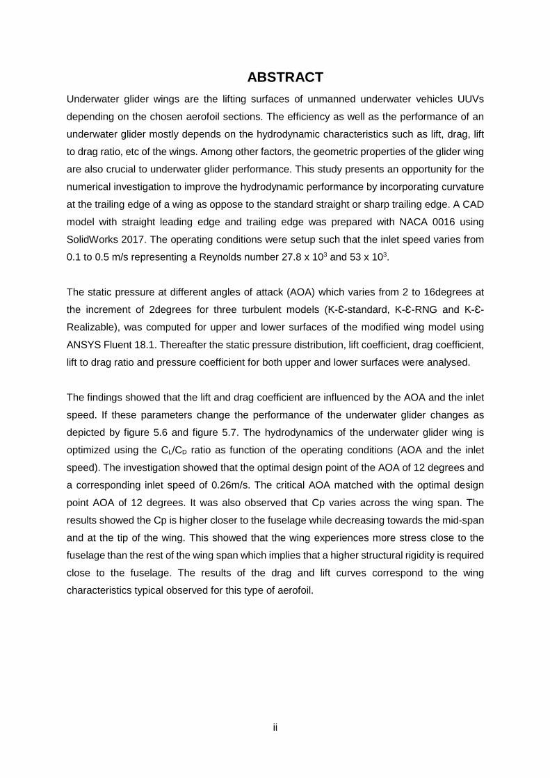
1.1 PROBLEM STATEMENT

Underwater gliders are self-propelled unmanned underwater vehicle with fixed wings that

convert vertical motion into horizontal motion, (Javaid et al., 2017). The vehicle has no external

propellers it gains its propulsion internally, by shifting negative to positive buoyancy using the

submarine mechanism, where it gains downward motion by additional mass or vice versa for

surfacing using piston pumps. Since the vehicle has no external propellers, the guide path is

controlled by external planes (wings) resulting in a trajectory of a sawtooth path or sinusoidal

as shown in figure1.1

2

Figure 1-1 Underwater glider operation-sawtooth path Bender et al., (2006)

Zhang et al., (2013), carried out an investigation on a simple non-standard trapezoid wing at

different wing aspect ratio (Zhang et al., 2013). The findings showed larger wings result in

shallow gliding path, longer horizontal travel with slow speed as compared to the smaller

wings. Liu et al., (2014), looked at the effect of the wing layout, specifically the influence of the

chord length, aspect ratio, sweep back angle and axial position. Their findings showed that

the chord length has a significant impact on the lift to drag ratio, while sweep angle has

significant impact on the movement of the underwater glider.

This present study looks at the effect of underwater glider wings geometric design with the

aim addressing the shortcomings experienced by current existing glider wings shapes as

mentioned above by introducing a Controlled Volume Computational Modelling technique to

compute the hydrodynamic forces acting on the glider wings.

1.2 BACKGROUND TO THE RESEARCH PROBLEM

At the end of world war two, designs of wings were of extreme importance, each institution

conducted their own investigation by testing various wing shapes and designs (Abbott,

n.d.).This process was carried out experimentally using wind tunnels in conjunction with

empirical methods. However due to the extraordinary and fine work done by NASA team, their

work was rated the most outstanding and reliable at that time (Abbott, n.d.). Since then most

traditional wing design were influenced by NACA’s pioneering work and their designs were

used as reference point. The traditional NACA wings designs shape has a round leading edge

and sharp trailing edge.

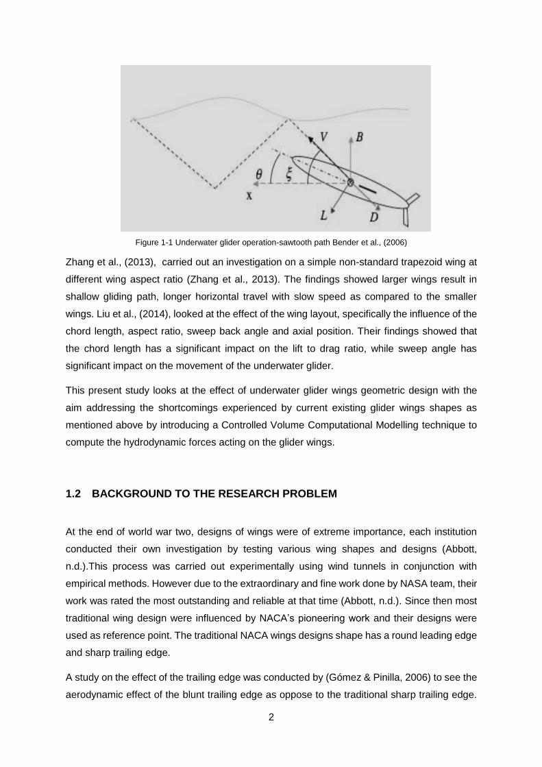
A study on the effect of the trailing edge was conducted by (Gómez & Pinilla, 2006) to see the

aerodynamic effect of the blunt trailing edge as oppose to the traditional sharp trailing edge.

3

The modification was parameterized by cutting the trailing edge perpendicular in different

sections along the chord length as depicted in figure 1.2. The findings showed an increase in

the maximum lift coefficient, profile drag and lift coefficient slope.

Figure 1-2 Modified NACA4412 aerofoil (Gómez & Pinilla, 2006)

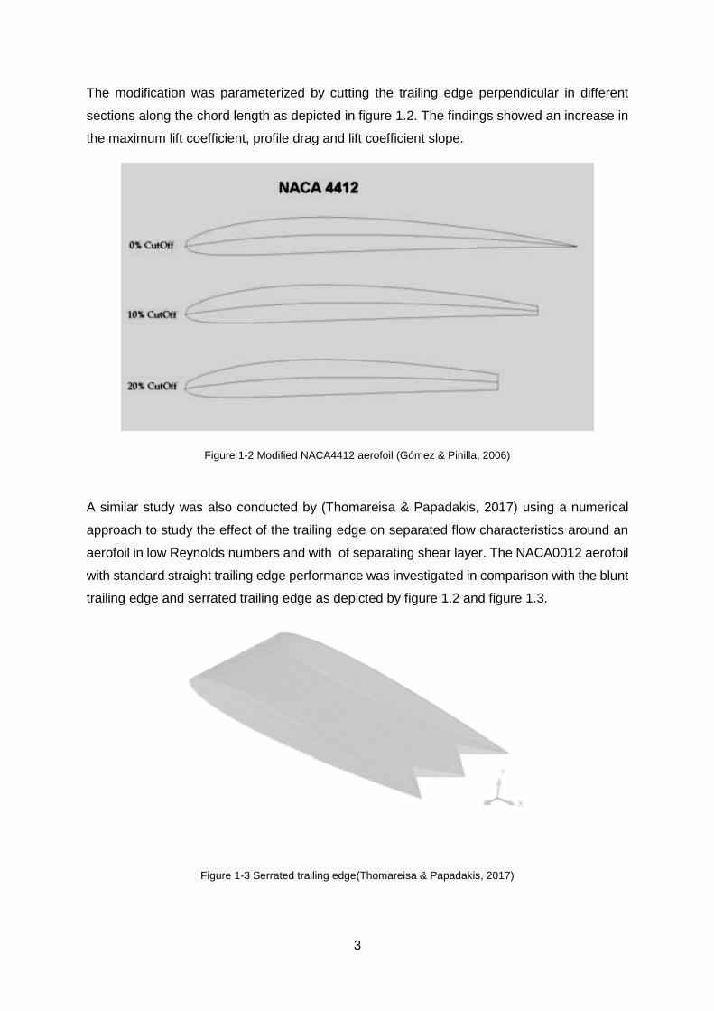
A similar study was also conducted by (Thomareisa & Papadakis, 2017) using a numerical

approach to study the effect of the trailing edge on separated flow characteristics around an

aerofoil in low Reynolds numbers and with of separating shear layer. The NACA0012 aerofoil

with standard straight trailing edge performance was investigated in comparison with the blunt

trailing edge and serrated trailing edge as depicted by figure 1.2 and figure 1.3.

Figure 1-3 Serrated trailing edge(Thomareisa & Papadakis, 2017)

4

The findings showed that the traditional straight-line standard aerofoil recorded two modes:

High frequency which corresponds to Kelvin Helmholtz instability originating from the

separated shear layer and low frequency which emerges as a sub-harmonic, detectable at the

suction side and near the wake.

The blunt trailing edge showed two shear layer frequencies which are strongly suppressed

and the frequency of the shear layer is locked to the shedding frequency due to exposed

bluntness. Serrated trailing edge which consist of triangular serration as shown in figure 1.3.

The strength of the vortices shed from the exposed blunt part is strongly attenuated compared

to the flatback aerofoil and this results in the presence of both sub-harmonic and shedding

frequency in the velocity spectra in the wake as well as in the suction side of the aerofoil

Xie et al., (2013) undertook a similar study looking at the effect of the incident angle on the

gliding distance of the glider. The smaller the gliding angle the longer the gliding distance, but

due to the relationship between the gliding angle and the wing incident angle, it is not easy to

measure the gliding angle directly (Xie et al., 2013). Thereafter, passively rotatable wings were

proposed. The findings showed that the passively rotatable wings can achieve a longer range

than the conventional fixed-wings if the incident angle is set properly.

The investigation of aerofoil has been reported in many studies whereby flapping, blunt and

serrated trailing edges were investigated with the aim of gaining lift and reducing drag.

However, there are very few studies on the effect of the round trailing edge on the

hydrodynamic performance of the underwater glider. This study is structured according to the

work conducted by (Javaid et al., 2016) where they looked at the effect of the wing form on

the hydrodynamics of the underwater glider i.e. tapered and rectangular wing using standard

NACA0016 aerofoil. This study looks at the effect of the rectangular wing form with round

trailing edge as opposed to the standard straight or sharp trailing edge, using the standard

NACA0016 as well. The investigation looks at the influence of the inlet speed and angle of

attack (AOA) on the hydrodynamic parameters such as coefficient of lift (CL), coefficient of

drag (CD), coefficient of pressure and the drag polar (CD/CL)) as a result of the geometric

modification of the trailing edge of the underwater glider wing.

1.3 AIM

The aim of the study is to find alternatives wing shapes that can improve the performance of

the underwater glider as oppose to the current traditional sharp trailing edge wing form.

5

1.4 OBJECTIVES

The main objectives of this thesis are to investigate the hydrodynamic performance of the

glider wing using the coefficient of lift (CL), coefficient of drag (CD), coefficient of pressure (Cp)

and drag polar (CD/CL) as parameters of interest.

1.5 STRUCTURE OF THE THESIS

CHAPTER 1

This chapter introduce the research, background to the research problem, aim of the project

and its objectives and lastly gives the layout of the thesis.

CHAPTER 2

Chapter two covers the literature review of the research area, underwater robots,

oceanographic engineering, the classification of autonomous Underwater Vehicles (AUV’s)

and the numerical and experimental studies on the wings form.

CHAPTER 3

Chapter three covers basic mathematical concept of CFD looking at the governing equations,

overview of the Computational Fluid Dynamics (CFD), numerical methods, turbulence and

hydrodynamic models.

CHAPTER 4

Chapter four’s focus is on the research methodology which discuss the glider wing geometric

design, flow domain creation, the computational mesh, brief theoretical considerations on thin

aerofoil and wings, turbulence resolutions and lastly numerical solutions.

6

CHAPTER 5

Chapter five covers the discussions of the results using qualitative and quantitative plots

respectively.

CHAPTER 6

This chapter covers the conclusions on the findings and possible recommendations for

future work.

7

CHAPTER 2

LITERATURE REVIEW

The study of the ocean became more popular since 19th century where the interest to explore

the ocean treasure grew stronger. As we all know the danger of the ocean to human kind,

scientist used sensors and floats to collect data but the shortcomings with this approach was

the range, duration and man power requirements. This forced the oceanographers to explore

the use of underwater vehicles. Underwater vehicles are small robots deployed from the ship

into the ocean with predefined mission based on the payload. Underwater vehicles are

designed with the intension to complete three tasks namely oceanographic sampling,

exploration and observation (Raj et al., 2014).

These class of vehicles are subdivided into, Autonomous Underwater Vehicle (AUV),

Remotely Operated Underwater Vehicle (ROV) and Underwater Glider (UG). This study will

be focusing more on underwater gliders.

2.1 BACKGROUND OF UNDERWATER GLIDERS

In 1989, Oceanographer Henry Stommel envisioned a future of underwater robots, working in

a group, autonomously powered by a sort of buoyant energy. This vision was put forward by

other oceanographers in 2001, three underwater gliders were developed by three different

institutions. Doug Webb and his team via Webb Research Cooperation developed two types

of Slocum underwater gliders (electrically powered and thermal powered). Scripps Institution

of oceanography developed Spray underwater glider named after Joshua Slocum sail boat by

honouring the first brave man to sail around the world in small boat and University of

Washington developed Sea glider (Hussain et al., 2011). The detailed specifications of the

three popular underwater gliders are shown in table 2.1.

8

Table 2-1 Comparison of specifications between Spray, Slocum and Seaglider (Davis et al., 2002)

Spray Specifications

Hull Length 2m, Diameter 0.2m, Mass 51 kg, Payload 3.5 kg

Lift Surfaces Wing span (Chord) 1.2 (0.1) m, Vertical stabilizer length (chord) 0.49(0.07) m

Volume

Change

Max 900 cc, Motor & reciprocating pump, 50 (20) % efficient @1000(100) dbar

Communication Iridium, 180 byte/s net, 35 J/Kbyte. GPS navigation

Operating Max P 1500 dbar, Max U 45 cm/s, Control on depth+altitude+vertical W

Endurance U = 0.27m/s, 180 glides, Buoyancy 125 gm, Range 7000 km, Duration 330 days

Slocum

Hull Length 1,5m (overall 215), Diameter 0.21m, Mass 52kg, Payload 5 kg

Lift Surfaces Wing span (chord) 1.2 (0.09) m swept 450, Stabilizer length (chord) 0.15 (0.18) m

Volume

Change

Typical 450 cc, 90 W motor & single-stroke pump, 50% efficient @200 dbar

Communication Freewave LAN,5.7 Kbytes/s, 3 J/Mbyte, 30 km range – or –Iridium, GPS

navigation

Operating Max P200 dbar, Max U 0.4m/s, Control on depth+altitude+altitude+vertical W

Endurance U = 0.35m/s, 250 glides, Buoyancy 230 gm, Range 500 km, Duration 20 days

Seaglider

Hull & Shroud Length 1.8 m(Overall3.3), diameter 0.3m, Mass 52kg, Payload 4kg

Lift Surfaces Wing span (av chord) 1(0.16) m, Vertical stabilizer span (chord) 0.4 (0.07) m

Volume

Change

Max 840 cc, Motor & reciprocating pump,40% (8%) efficient at 1000(100) dbar

Communication Iridium,180 bytes net, 35J/Kbytes, GPS navigation

Operating Max P 1000 dbar, Max U 0.45m/s, Control on depth+position+attitude+vertical W

Endurance U= 0.27 m/s, 160 glides, buoyancy 130gm, Range 4600 km, Duration 200days

Underwater gliders are self-propelled unmanned underwater vehicle with wings that convert

vertical motion into horizontal motion, Javaid, M.Y, et al., (2016). The vehicle has no external

propellers it gains its propulsion internally, by shifting negative to positive buoyancy using the

submarine mechanism, where it gains downward motion by additional mass or vice versa and

for surfacing use piston pumps or ballast tanks. Since the vehicle has no external propellers

manoeuvrability is largely by external planes(wings). This then result in a trajectory of a

sawtooth path or sinusoidal motion. Bender and his colleagues (Bender et al., 2008),

describes underwater gliders as a type of autonomous submersibles vehicles with an

approximate length of 2 metres, weighing 50 kilograms and resembling sailplanes as shown

9

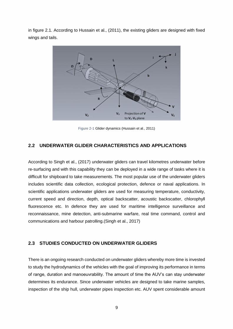
in figure 2.1. According to Hussain et al., (2011), the existing gliders are designed with fixed

wings and tails.

Figure 2-1 Glider dynamics (Hussain et al., 2011)

2.2 UNDERWATER GLIDER CHARACTERISTICS AND APPLICATIONS

According to Singh et al., (2017) underwater gliders can travel kilometres underwater before

re-surfacing and with this capability they can be deployed in a wide range of tasks where it is

difficult for shipboard to take measurements. The most popular use of the underwater gliders

includes scientific data collection, ecological protection, defence or naval applications. In

scientific applications underwater gliders are used for measuring temperature, conductivity,

current speed and direction, depth, optical backscatter, acoustic backscatter, chlorophyll

fluorescence etc. In defence they are used for maritime intelligence surveillance and

reconnaissance, mine detection, anti-submarine warfare, real time command, control and

communications and harbour patrolling.(Singh et al., 2017)

2.3 STUDIES CONDUCTED ON UNDERWATER GLIDERS

There is an ongoing research conducted on underwater gliders whereby more time is invested

to study the hydrodynamics of the vehicles with the goal of improving its performance in terms

of range, duration and manoeuvrability. The amount of time the AUV’s can stay underwater

determines its endurance. Since underwater vehicles are designed to take marine samples,

inspection of the ship hull, underwater pipes inspection etc. AUV spent considerable amount

10

of time underwater without refuelling or charging hence a good propulsion technique, better

speed and energy source is needed (Raj & Chandra, 2014).

Underwater gliders have no propulsion power which makes it unique compared to other AUV

and with better endurance (Hussain et al., 2011). The lack of propulsion power result in less

energy usage making it possible to operate at much deeper depth, like the sea glider. This

type of underwater vehicle has low drag hull with high lift to drag ratio. Therefore the proper

wing configuration is crucial to minimise the drag and optimise energy consumption.(Singh et

al., 2017)

There are different approaches used to study the hydrodynamics of this vehicle but with the

advances in computational power, the most common approach is by numerical simulation

using (CFD) platform validated by experimental data.

2.3.1 The influence of the wing shape on lift and drag characteristics

2.3.1.1 Theory of wings

The systematic tests were done by National Advisory Committee for Aeronautical (NACA) on

various shapes of the aerofoils generating data for aircraft design. Although these test were

conducted many decades ago but are still used as the reference guide even today when

designing certain components of the aircraft.(Anon, n.d.) The NACA produced different family

of wings , ranging from 4- digit ,5 digit and 6-digit aerofoils. The specifications of these wings

are shown in table 2.2.

Table 2-2 Classification of different NACA family of wings (Anon, n.d.)

Series type NACA Type Camber max Thickness max

4 digits NACA2415 0.02% over the chord 0.15c

5 digits NACA23021 0.02% over the chord 0.12c

6 digits NACA63215 - 0.15c

The shape of the standard NACA wing follows a round leading edge (LE) and a sharp trailing

edge (TE) as mentioned in section 1.3. Since the work deals with the four-digit wing, the

numbering system for the four-digit series is based on the section geometry. The first integer

indicates the maximum value of the mean-line coordinate in percent of the chord while the

second integer represent the distance from the LE to the maximum camber in tenths of the

chord. The last two integers indicate the section thickness in percent of the chord. In cases of

11

the NACA 0016, this type of wing is symmetrical due to the first two zero’s in front sections

and the last two integers represents the percentage thickness. (Abbott, n.d.)

2.3.1.1.1 Wing aspect ratio

The wing aspect ratio is known as the wing span divided by the geometric chord or it can be

described as the measure of how long and narrow the wing is.(Anon, n.d.).The formula to

calculate the aspect ratio is given by equation 2.1.

𝐴𝑅 =𝑏

𝑐=

𝑏2

𝑆 (2.1)

The early wind tunnel test showed the rate of change of the lift and drag coefficients as a

function of the AOA are strongly affected by the aspect ratio of the model.(Abbott, n.d.).

2.3.1.2 Experimental approach

This study deals with external flow around underwater glider wing. The nature of the flow in

the fluid is determined by the Reynolds number. This parameter is a function of speed, density,

viscosity and the surface area as shown by equation.

𝑅𝑒 =𝜌𝑣𝑑

𝜇 (2.2)

According Hussain and his team (Hussain et al., 2011), underwater gliders speed ranges

between 0.25 m/s to 0.5 m/s. The nature of the speed of the underwater gliders in respect to

equation 2.2 suggest that the flow around these vehicles is turbulent. The flow in this region

is chaotic and three dimensional and results in fluctuating flow behaviour. Since this study

deals with external flow, there are ample studies conducted on hydrodynamics characteristics

around underwater gliders with the aim of improving the performance in terms of range,

endurance, stability and reduction of the operating cost. The primary focus of this chapter will

be directed towards the influence of the wing form shape on the hydrodynamic characteristics

of the underwater glider.

(Dod, 1946), conducted an experimental study on a wind tunnel for various NACA 44 series

wings looking at the aspect ratio, taper ratio and overall surface finish of the wing. His

approach used the experiment data to validate the computed aerodynamics characteristics of

the wings. The calculations were carefully done by considering different methods which use

12

lifting-line theory which assumes linear section of lift curves and the non-linear lift curves

theory.

The findings for both methods of calculation showed reasonable agreement with the

experiment data for the wing force (drag) and the moment characteristics. However, the

method that allows the use of nonlinear lift curves gave better agreement with the experiments

at high AOA. The only point where both methods gave different results was on the span wise

lift distributions at maximum lift. The results also compared the drag and lift force at an equal

Reynolds number for all the conditions and the findings showed that the lift to drag ratio for

smooth wings increased with the increasing aspect ratios throughout the wing span

irrespective of the increase in drag due to the increasing root thickness at higher aspect ratios.

The (L/D) max, for the taper ratio of 3.5 with rough leading-edge surface yielded the same trend

with smooth surface wings, however for the taper ratio of 2.5 with same surface finish showed

no gain when the aspect ratio was increased from 10 to 12. Lastly, the maximum lift coefficient

decreased with increasing aspect ratio due to the increase in root thickness to chord ratio.

Haque et al.,(2015) conducted a similar study where they performed a test experimentally on

NACA 4412 using wind tunnel (Haque et al., 2015). The test compared the aerodynamic

performance by incorporating a curvature in the leading-edge while maintaining the straight

trailing edge in comparison with a rectangular straight leading-edge and straight trailing-edge

as shown in figure 2.2.

Figure 2-2 (a) Curved Leading Edge Planform (b) Rectangular Planform (Haque et al., 2015)

The findings show the curved leading-edge wing planform exhibit high lift coefficient and lower

drag coefficient than the rectangular wing planform. This also result in curved leading-edge

planform having higher lift to drag ratio than the rectangular planform. The other finding

showed the pressure coefficient is independent of the chord length, by displaying the variation

of the Cp while maintaining the chord length constant.

13

Hossain et al.,(2011) conducted an experiment on aerodynamic characteristics of the

rectangular wing with and without bird feather like winglets for different Reynolds Numbers

(Hussain et al., 2011). The findings showed 25-30% reduction in Cd and 10-20% increase in

Cl for the bird feather like winglet at AOA of 8 degrees. Dwivedi et al., (2018) also adopted an

experimental approach in studying different wing shapes i.e. Rectangular, rectangular with

curved tip, tapered, tapered with curved tip for low speed at various AOA. The findings showed

tapered wing with curved tip exhibit the best aerodynamic stability for various speed and

AOA(Dwivedi et al., 2018).

2.3.1.3 Numerical approach

The lift generated by the wing sustains the weight of the underwater glider to sustain its motion

in water. There are different numeral approaches used to investigate the influence of the wing

form using different Computational Fluid Dynamics (CFD) platforms. According to Lynch

(1982) around two thirds of the total drag of the aircraft or submersible is produced by wings

hence the wing form shape is very crucial to the performance of a glider.

A numerical study was conducted by (Ahmed, 2013) looking at the flow around a NACA0012

wing flapped at different flap angles with varying Mach Numbers. The study used k-ω shear

stress transport (SST) turbulence model to predict the flow accuracy along with turbulence

intensities 1% and 5% at different inlet velocities and pressure outlet respectively. The findings

showed that the calculation of CL, CD and CL/CD ratio at different operating conditions with the

increase in Mach number, CL increases whereas CD remain constant. It was also noticed as

the speed approaches sonic velocity, a rapid decrease in CL was observed whereas an abrupt

upsurge was observed for CD.

A study by Arvin et al.,(2016) on 3D simulation of turbulent flow over three different aerofoils

(NACA 680094 ,NASA-GAW2 and a designed aerofoil) was conducted (Arvin et al., 2016).

Two computational platforms: ANSYS-fluent and XFLR5-V609 were used to carry out the

investigation looking at the effect of Moment coefficient (Mc), CL and drag coefficient CD for

various AOA and Reynolds numbers. The findings showed that the designed aerofoil exhibit

similar behaviour with the standard aerofoil for different AOA and resulting CL / CD ratio at AOA

of 5 degrees.

Rahimi et al.,(2014) undertook a study on numerical investigation of 2D and 3D for different

aerofoils at Laminar and Turbulent flow conditions using Open FOAM (Rahimi et al., 2014).

14

The findings showed good agreement when compared to the experimental data and other

numeral results for both Open FOAM transition model and k-ω (SST).

Jones & Clarke,2005 conducted a numerical study using the CFD code (Fluent) to cary the

investigation of horseshoe vortex formed in a typical wing junction in a turbulent flow

experiment using various turbulent models i.e. k-Ԑ (RNG) ,Reynolds stress model(RSM ,V2F

model, Spallart – Allmaras model and k-ω model.The findings showed ,the k-Ԑ (Realizable)

model predictions is less accurate when compared to all other models for mean velocity

compents.None of the models predicted accuratetly the behavior of the mean kinetic energy

as a function of the domain extent although for time averaged velocity components most

locations the models predicited these components accurately.

A numerical simulation of the aerofoil flow at high AOA was conducted by (Panaras, 2015).The

study look at different turbulent models i.e linear k-ω (SST), non-linear algebraic Stress Model

and Baldwin-Lomax model. The findings showed that the tested models captured the physics

of unsteady seperated flow.Good agreement between computational and experimental

surface pressure data was also observed.

According to Azim et al.,(2015) the flow separation at the trailing edge of the aerofoil affects

the aerodynamic perfomance significantly (Azim et al., 2015).For instance, a decrease in the

lift whilst increasing the drag.Their study looked at the boundary layer separation using 2D

NACA 4412 model by introducing suction on the aerofoil and use CFD to compute the

numerical results.The right suction position is paramount and therefore the aerofoil was slotted

with a width of 2% of the chord length in five different positions starting from 48% to 70% of

the chord length.The findings showed that if the suction pressure is kept at 65 kpa at 68% of

the chord length at the AOA = 13 degrees, it is possible to arrive at an optimal position where

the suction inside the aerofoil works best. The delay in the onset of the turbulent flow ultimately

results in an increase in the lift.

In a simlar study (van de Wal, 2010), studied the design of the wing with boundary layer suction

with the aim of reducing the profile drag.The study designed a completely new aerofoil in

XFOIL and optimized the design for boundary layer suction.The new aerofoil produced good

results with or without suction and reduced the profile drag tremendously while on the other

hand the lift coefficient increased dramatically.

In another investigation (Fulvio Bellobuono Tutor Coordinator Domenico Coiro Antonio

Moccia, 2006), a study was conducted on exploring different ways of achieving efficient

boundary layer control, with an awareness of the practical implications when installing the

device on the actual wing.The study also look at the verification of the existing active control

steady suction and pulse blowing to see which one is effective in terms of boundary layer

15

separation.The findings showed that the steady suction is an effective tool for delaying the

boundary layer seperation, but it is a function of the position of the slot, whereas the numerical

and experimental test showed that the unsteady blowing is more effective than the steady

blowing.

2.4 SUMMARY

Looking at the litearture that has been reviewed in this chapter, it became evident that there

is very minimal work done around the subject of optimization of underwater glider wings.This

has brought the need of studying the effects of hydrodynamic perfomance of an underwater

glider looking at the effect of modifying the trailing edge of the underwater glider wing.The

recent Literature has revealed that most work has been perfomed through the analysis of the

perfomance of the entire wing shapes i.e. Tappered wings against rectangular

wings,perforated wing using active control steady suction and pulse blowing. This work is

analysing the effect of modifying the trailing edge of the recctangular NACA0016 wing shape.

16

CHAPTER 3

COMPUTATIONAL FLUID DYNAMICS (CFD)

Computational Fluid Dynamics (CFD) is the branch of Fluid mechanics that deals with the

analysis of systems involving fluid flow, heat transfer and associated phenomena such as

chemical reactions by means of computer-based simulation. The technique is very powerful

and widely used in many academia, industries and in non-industrial applications. In the early

1960s aerospace extended the capability of the technique to iterate the design, research and

development (R&D) and overlapping functions to the manufacturing of aircraft and jet engines.

3.1. GOVERNING EQUATIONS

The principles of conservation of mass, energy and momentum are used to derive the

fundamental equations necessary to describe the behaviour of any fluid flow. Since this work

deals with incompressible fluid it is assumed that solving the energy equation will have no

significant effect on the solution, therefore the heat transfer during the fluid flow is neglected

to simplify the problem.

The governing equations for incompressible flow are based on the conservation equations of

mass and momentum. These equations which are solved using numerical methods is given

in a three-dimensional differential form as shown below (Versteeg and Malasekera, 2007).

3.1.1 Mass conservation equation

The three-dimensional mass conservation for incompressible fluid is given by equation (3.1).

𝜕𝑢

𝜕𝑥+

𝜕𝑣

𝜕𝑦+

𝜕𝑤

𝜕𝑧= 0 (3.1)

where 𝑢 =𝑑𝑥

𝑑𝑡; 𝑣 =

𝑑𝑦

𝑑𝑡 𝑎𝑛𝑑 𝑤 =

𝑑𝑧

𝑑𝑡 are the velocities in the different positions of the three-

dimensional axis x, y and z.

Equation (3.1) in more compact vector notation is given by equation (3.2)

div 𝐮 = 0 (3.2)

where div 𝐮 =𝜕𝑢

𝜕𝑥+

𝜕𝑣

𝜕𝑦+

𝜕𝑤

𝜕𝑧

17

3.1.2 Momentum conservation equation

The momentum conservation equation is shown by equation (3.3).

𝐷𝜑

𝐷𝑡=

𝜕𝜑

𝜕𝑡+

𝜕𝜑

𝜕𝑥

𝑑𝑥

𝑑𝑡+

𝜕𝜑

𝜕𝑦

𝑑𝑦

𝑑𝑡+

𝜕𝜑

𝜕𝑧

𝑑𝑧

𝑑𝑡 (3.3)

Equation 3 can also be written as shown in equation (3.4)

𝐷𝜑

𝐷𝑡=

𝜕𝜑

𝜕𝑡+ 𝑢

𝜕𝜑

𝜕𝑥+ 𝑣

𝜕𝜑

𝜕𝑦+ 𝑤

𝜕𝜑

𝜕𝑧=

𝜕𝜑

𝜕𝑡+ 𝒖. 𝑔𝑟𝑎𝑑𝜑 (3.4)

where 𝑔𝑟𝑎𝑑𝜑 =𝜕𝜑

𝜕𝑥+

𝜕𝜑

𝜕𝑦+

𝜕𝜑

𝜕𝑧=

𝜕𝜑

𝜕𝑡

Therefore, the x-momentum, y-momentum and z-momentum for incompressible flow then

becomes:

𝜕𝑢

𝜕𝑡+ div(𝑢𝐮) = −

1

𝜌

𝜕𝑝

𝜕𝑥+ 𝑣 div(𝑔𝑟𝑎𝑑(𝑢)) (3.5)

𝜕𝑣

𝜕𝑡+ div(𝑣𝐮) = −

1

𝜌

𝜕𝑝

𝜕𝑦+ 𝑣 div(𝑔𝑟𝑎𝑑(𝑣)) (3.6)

𝜕𝑤

𝜕𝑡+ div(𝑤𝐮) = −

1

𝜌

𝜕𝑝

𝜕𝑧+ 𝑣 div(𝑔𝑟𝑎𝑑(𝑤)) (3.7)

3.2 CFD MODELLING TECHNIQUES

In general, there are three computational approaches available to model the behaviour of

turbulent flow namely: Direct Numerical Simulation (DNS), Large Eddy Simulation (LES) and

Reynolds Average Navier-Stokes Simulation (RANS). A brief explanation of each approach

will be discussed and closed off with a numerical approach suitable for the nature of the

problem investigated.

3.2.1 Direct numerical approach (DNS)

Direct numerical simulation computes both the mean flow and all turbulent velocity

fluctuations. The unsteady Navier -Stokes Equations are solved on spatial grids that are

sufficiently fine, enable to resolve the Kolmogorov length scales at which energy dissipation

takes place with time steps sufficiently small to resolve the period of the fastest fluctuation.

This approach is computationally prohibitive and not practical for the industrial flows hence, it

is not considered for practical reasons (Versteeg and Malasekera, 2007)

18

3.2.2 Large eddy simulation (LES)

Large Eddy Simulation is regarded as the intermediate form of turbulence calculations which

tracks the behaviour of large eddies. The method involves space filtering of the unsteady

Navier-Stokes equations prior to the computations, which captures the larger eddies and reject

the smaller eddies. The effects on the resolved mean flow, plus large eddies due to the

smallest unresolved eddies are included by means of sub-grid scale model. Since the

unsteady flow must be solved then the demand on the computation resources and storage

becomes enormous (Versteeg and Malasekera, 2007). Although this technique is starting to

address CFD problems when dealing with complex geometries, it still beyond the limit of

resources available for a basic CFD study.

3.2.3 Reynolds Average Navier-Stokes Simulation (RANS)

Reynolds Average Navier -Stokes approach to turbulence modelling is focused on the mean

flow and the effects of turbulence on the mean flow properties. Prior to the application of

numerical methods, the Navier-Stokes equations are time averaged. The extra term that

appear in the time averaged flow equations is due to the interactions between various turbulent

fluctuations and they are modelled with classical turbulent models e.g. k-Ԑ models and

Reynolds stress model. (Versteeg and Malasekera, 2007)

This approach is widely used for most industrial flows and since in practice, underwater gliders

operates at very low speeds ranging from 0.25m/s to 0.5m/s, at the corresponding Reynolds

number of between 1 x 105 to 1 x 106; Zhang et al.;(2013), RANS equation becomes readily

application in this situation. (Jagadeesh et al., 2009), recommends the use low Reynolds

turbulence models such as the RANS equation for incompressible flow as proposed by (Javaid

et al., 2017) when dealing with underwater gliders. The classical eddy-viscosity turbulence

models are used to resolve the turbulence terms in Reynolds Averaged Navier-Stokes

equations.

19

3.3 TURBULENT FLOW

In general, flow over external bodies is considered turbulent when the Reynolds number is

greater than (Re>5x105). Turbulent could be thought as instability to the laminar flow at high

Reynolds numbers (Re). These instabilities origin form interaction between non-linear inertial

terms and viscous terms in Navier-Stokes equation. The nature of these interactions is

rotational, fully time dependent and three dimensional as shown in figure 3.1. In true essence,

rotational and three-dimensional interactions are connected through vortex stretching. It is

almost impossible to obtain vortex stretching in two-dimensional space, hence most

satisfactory approximations are three dimensional.

Figure 3-1 Growth of turbulent spots in a flat plate boundary layer(Nichols, n.d.)

Since this study focus on underwater gliders, the dimensions and velocities of typical

underwater gliders are such that the Reynolds number is greater than 1.0 x106 which falls

within the low turbulent flow regime as given in equation 2.1.

The initial speed of the underwater glider given as 0.1 m/s and the theoretical calculation

showed that underwater gliders due to the nature of their speed they operate at low turbulent

zone. Numerically turbulent flow simulation equations are solved for a time-independent

velocity field that represents the velocity field 𝑈(𝑥, 𝑡) (Anon ,2000:362).

20

3.3.1 Turbulence modelling

Three two-equation models’ predictions of the hydrodynamics and flow field are compared to

see the model that can closely predict the physics of the problem. The models used are k-ԑ

model (Standard), k-ԑ model (RNG) and k-ԑ model (Realizable). The k-term focuses on the

mechanisms that affect the turbulent kinetic energy whereas ԑ-term focuses on turbulent

dissipation rate. The instantaneous kinetic energy of a turbulent flow is then given by the sum

of the mean kinetic energy as shown in equation 8.(Versteeg and Malasekera, 2007)

𝑘(𝑡) = 𝐾 + 𝑘 (3.8)

where 𝐾(𝑡) =1

2(𝑈2 + 𝑉2 + 𝑊2) and 𝑘 =

1

2(𝑢′2̅̅ ̅̅ + 𝑣′2̅̅ ̅̅ + 𝑤′2̅̅ ̅̅ ̅)

The governing equation for mean flow kinetic energy k can be written as shown in

equation (3.9)

𝜕(𝜌𝐾)

𝜕𝑡+ div(𝜌𝐾𝐔) = div(−𝑃𝐔 + 2𝜇𝐔𝑆𝑖𝑗 − 𝜌𝐔𝑢𝑖

′𝑢𝑗′̅̅ ̅̅ ̅̅ ) − 2𝜇𝑆𝑖𝑗. 𝑆𝑖𝑗 + 𝜌𝑢𝑖

′𝑢𝑗′̅̅ ̅̅ ̅̅ . 𝑆𝑖𝑗 (3.9)

The governing equation for the turbulent kinetic energy k is given by equation 10

𝜕(𝜌𝐾)

𝜕𝑡+ div(𝜌𝐾𝐔) = div (−𝑝′𝐮′̅̅ ̅̅ ̅̅ + 2𝜇𝐮′𝑠′

𝑖𝑗̅̅ ̅̅ ̅̅ ̅ − 𝜌

1

2𝐮𝒊

′. 𝑢𝑖′𝑢𝑗

′̅̅ ̅̅ ̅̅ ̅̅ ̅) − 2𝜇𝑆′𝑖𝑗. 𝑆′

𝑖𝑗̅̅ ̅̅ ̅̅ ̅̅ ̅̅ − 𝜌𝑢𝑖

′𝑢𝑗′̅̅ ̅̅ ̅̅ . 𝑆𝑖𝑗 (3.10)

The k-ԑ model uses the following transport equations for k and ԑ given in equation (3.11) and

(3.12) respectively.

𝜕(𝜌𝐾)

𝜕𝑡+ div(𝜌𝐾𝐔) = div [

𝜇𝑡

𝜎𝑘𝑔𝑟𝑎𝑑𝑘] + 2𝜇𝑆𝑖. 𝑆𝑖𝑗 − 𝜌휀 (3.11)

where 𝜇𝑡 = 𝜌𝐶𝜇𝑘2

𝜀

𝜕(𝜌𝜀)

𝜕𝑡+ div(𝜌휀𝐔) = div [

𝜇𝑡

𝜎𝜀𝑔𝑟𝑎𝑑휀] + 𝐶1𝜀

𝜀

𝑘2𝜇𝑡𝑆𝑖𝑗. 𝑆𝑖𝑗 − 𝐶2𝜀𝜌

𝜀2

𝑘 (3.12)

Since this study used k-Ԑ(RNG) model, the equations for k and ԑ for the model is given by

equation (3.13) and equation (3.14) respectively.

𝜕(𝜌𝜀)

𝜕𝑡+ div(𝜌𝐾𝐔) = div[∝𝑘 𝜇𝑒𝑓𝑓𝑔𝑟𝑎𝑑 𝑘] + 𝜏𝑖𝑗 . 𝑆𝑖𝑗 − 𝜌휀 (3.13)

𝜕(𝜌𝐾)

𝜕𝑡+ div(𝜌휀𝐔) = div[∝𝜀 𝜇𝑒𝑓𝑓𝑔𝑟𝑎𝑑 휀] + 𝐶1𝜀

∗ 𝜀

𝑘𝜏𝑖𝑗 . 𝑆𝑖𝑗 − 𝐶2𝜀𝜌

𝜀2

𝑘 (3.14)

where 𝜏𝑖𝑗 = −𝜌𝑢𝑖′𝑢𝑗

′̅̅ ̅̅ ̅̅ = 2𝜇𝑡𝑆𝑖𝑗 −2

3𝜌𝑘𝛿𝑖𝑗 and 𝜇𝑒𝑓𝑓 = 𝜇 + 𝜇𝑡

𝐶𝜇 = 0.0845 𝛼𝑘 = 𝛼𝜀 = 1.39 𝐶1𝜀 = 1.42 𝑐2𝜀 = 1.68

21

3.4 NUMERICAL METHOD

Numerical solution is obtained following different numerical steps as discussed below.

3.4.1 Computational domain

The computational fluid domain is described as the boundary or a fluid zone that depicts a

real-life scenario or environment of the problem. Usually the target object of interest is placed

inside the domain positioned categorically by following guidelines as detailed in section 5.3.

The computational fluid domain can be created in many ways depending on the choice of the

end user. In this study, the computational fluid domain is created using a proprietary CAD

software (Solidworks 2017, Dassault Systemes), then imported to ANSYS work bench 18.1.

The next step was the discretisation of the computational fluid domain referred to as meshing.

3.4.2 Mesh (general overview)

In numerical approach, one has to define the problem in a manner that is easy to compute by

looking at the surfaces, boundaries, spaces around the computational domain and break it

down into small infinitesimal cells or elements. This process is termed meshing or

discretisation. In general, as shown in figure 3.5 there are three major aspects of discretisation

when solving fluid flow problems namely: Equation discretisation, Spatial discretisation and

Temporal discretisation.

Figure 3-2 Discretisation of flow in CFD

22

3.4.2.1 Equation discretisation

Equation discretisation is carried out in numerical simulation using three methods: finite

difference method (FDM), finite element method (FEM) and Finite volume method (FVM).

3.4.2.1.1 Finite difference method

Finite difference methods apply Taylor expansion method to solve second partial differential

equations (PDEs) of the governing equation for fluid flow. The method arranges the derivatives

of the PDEs and write them in discrete quantities of variables yielding simultaneous algebraic

equations, with unknowns defined at the nodes of the mesh. FDM gained its popularity due to

its simplicity and ease in obtaining higher order accuracy discretisation. However, FDM has

limitation such that it can only be applied on simple geometries as it requires structured mesh.

3.4.2.1.2 Finite element method

Finite element method has the ability to solve complex geometries as it employs unstructured

mesh, where a computational domain is divided into finite number of elements and within each

element, a certain number of nodes are defined and the numerical values of the unknown are

determined. In finite element method, the discretisation is obtained using the method of

weighted residuals, that approximate the solution to a set of partial differential equations using

interpolation functions. However, this method requires high computing power compared to the

finite difference method

3.4.2.1.3 Finite volume method

This method integrates the governing equations for fluid flow and solve them iteratively based

on the conservation law on each control volume. This discretisation process results in a set of

algebraic equations that solves the variables at a specified finite number of points within the

control volumes, which then the flow around the domain can be modelled. This method can

employ structured and unstructured mesh. Since this method uses direct integration, it is more

efficient and easier to program in terms of CFD code development. This method uses less

23

computing power whereas it can solve simple and complex geometries and is more common

in recent CFD applications compared to FEM and FDM.

3.4.2.2 Spatial discretisation

Spatial discretisation divides the computational domain into small sub domain making up the

mesh. This defines each subdomain mathematically specifying its velocity at all points in space

and time. There are three different mesh types mainly used in CFD namely: structured,

unstructured and multi-block structured mesh. Structured mesh is built on a coordinate

system, commonly used in simple geometries such as square and rectangular. The structured

mesh performs badly when applied to complex geometries hence switch to the unstructured

mesh when dealing with complex geometries.

Unstructured mesh gives the allowance to rearrange elements and nodes on the

computational domain such that different kinds of complex geometries can be simulated. In

as much unstructured mesh works well with complex geometries it comes at a cost, as it

requires more computing power. In order to compensate for computing cost and flexibility,

multi-block structured or hybrid mesh is then deployed. Multi-block structured mesh generates

a mesh that consist of structured and unstructured mesh. However, it is very complicated to

generate a multi-block structured mesh as oppose to the structured mesh, but the multi-block

structured mesh gives control to refine sharp edges, corners and surfaces with suitable mesh

type, based on the complexity of the geometry.

3.4.2.3 Temporal discretisation

Temporal discretisation works with time, whereby it divides the time in a continuous flow into

discrete time steps. Transient or time dependent formulations, comprise of an additional time

variable t in the governing equations compared to the steady state analysis. This then leads

to a system of partial differential equations in time, which comprise of unknowns at a given

time as a function of the variables of the previous time step. Hence, unsteady simulation

requires longer computational time compared to a steady case due to the additional steps

between the equation and spatial discretisation.

24

3.5 SOLUTION METHODS

ANSYS Fluent have two solution methods available, pressure velocity-coupling and density-

based. Pressure velocity-coupling solves pressure and velocity simultaneously whereas

density-based method implements segregated approach where each variable pressure and

velocity are solved in series of time. In this study since we are solving for pressure and velocity

therefore pressure-velocity coupling method is used in this study.

3.6 HYDRODYNAMIC FORCES

In practice, it is always difficult to move a body through a fluid due to the resistance the fluid

to the motion of the body immersed in it and this phenomenon is called drag. It is important to

note that a stationary fluid exert only normal pressure forces on the surface of the submerged

body whereas a moving fluid exerts tangential shear forces on the surface because of no-slip

condition caused by viscous effects. This effect constitutes the basic hydrodynamic

interactions between a moving body and the fluid. Other interactions such as buoyancy and

gravitational forces are negligible and therefore not considered in this work. Both forces in

general have components in the direction of the stream flow thus drag force is regarded as

the combination of the effect of pressure and wall shear forces in the direction of the

flow.(Cimbala and Cengel, 2009)

These components are termed skin friction drag (due to shear forces on the surface) and form

drag (due to pressure normal to the flow direction acting in the frontal or projected area) as

shown in equation (3.15).

𝐹𝐷 = 𝐶𝐷𝐴𝜌𝑉2

2 (3.15)

where 𝑪𝑫 is the coefficient of drag, 𝑨 the projected area,𝝆 density of the fluid and 𝑽 free stream

flow velocity of the fluid.

The Lift force is considered as the components of the pressure and wall shear forces in the

normal direction but opposite gravitational force and is given by equation (3.16).

𝐹𝐿 = 𝐶𝐿𝐴𝜌𝑉2

2 (3.16)

Where 𝑪𝑳 is the coefficient of Lift, 𝑨 is the area normal to the force 𝝆 density of the fluid and

𝑽 stream flow speed of the fluid.

25

Surface pressure coefficient due to static pressure acting normal to the glider wing is given

by equation (3.17).

𝐶𝑃 =𝑃𝑖−𝑃∞

1

2𝜌𝑉2

(3.17)

Where 𝑃𝑖 is the surface static pressure

26

CHAPTER 4

COMPUTATIONAL FLUID DYNAMIC SETUP

4.1 GLIDER GEOMETRIC DESIGN

Several standard aerofoil shapes are frequently used in aerodynamic and hydrodynamic

designs. The most popular is the NACA aerofoil standard (Abbott, n.d.). In this study, a

standard NACA 0016 chosen after preliminary geometric designs considerations was modified

and evaluated. A numerical simulation was thereafter performed to evaluate the

hydrodynamics of the modified version of the NACA wing.

A computational model was developed to investigate the hydrodynamic behaviour of the

modified standalone NACA wing as opposed to the one that is attached on the fuselage of the

underwater glider under turbulent hydrodynamic conditions. The following tasks was carried

out in performing the analysis. This include geometry creation, computational mesh

generation, numerical solution and post processing.

Figure 4-1 Schematic illustration of the glider and the adapted/modified NACA wing (a) Glider model (b) Modified NACA 0016 wing

(a) (b)

27

4.1.1 Flow domain creation

Online NACA wing geometry point generator was used to download NACA0016, 2D aerofoil

geometry points. The geometry points are saved into a notepad then imported to Computer

aided draughting CAD software (Solidworks,2017) as shown in Table 4.1.

Table 4-1 Truncated geometry points of the overall NACA0016

Figure 4-2 2D scaled NACA0016 airfoil and modified CAD 3D wing

Figure 4.1 (a) shows a 2D model of the NACA0016 aerofoil. Using Solidworks CAD tools, the

2D model is modified further and converted into a 3D model as shown in (b). The overall

summary of the dimensions of the glider wing are shown in Table 4.2.

Table 4-2 Dimension of the glider wing

Dimensions Round trailing edge wing

Total wing span 300 mm Root Chord Length 170 mm Diameter of the wing 45 mm Taper Ratio - Sweep Angle 90 degrees

Points X Y Z

1 1mm 0mm 0mm

2 1mm 0mm 0mm

3 0.99mm 0mm 0mm

4 0.99mm 0mm 0mm

5 0.98mm 0mm 0mm

6 0.96mm 0.01mm 0mm

a b

28

The fluid domain is created following the guidelines of (Javaid et al., 2016). The ITTC

guidelines (Bertram, 2012) state an upstream boundary 1-2 times the length of the glider, and

the downstream boundary 3-5 times the length of the glider. (Zhang et al., 2013) and (Javaid

et al., 2016) conducted similar investigation on submerged bodies, with similar boundary

parameters, where the inlet flow was set to be 1.5 times the length of the glider and 3.5 times

away from the glider.

The ceiling and bottom wall were given as 9 times the diameter of the glider to avoid the error

effect caused by an interruption in the fluid flow. The solution domain for this work followed

the approach of (Javaid et al., 2017). The dimensions of the fluid domain are as follows:

upstream boundary is set at 2 times the length of the glider wing; downstream boundary is 4

times the length of the glider wing and from the ceiling-wall of the domain to the wing plane

and from the bottom wall domain to the wing plane is 9 times the glider wing diameter as

shown in figure 4.3.

4.1.2 Computational mesh

Multizone is selected as the method to generate the mesh. Since the multizone generate

structured mesh as shown in figure 4.4, it was then easy to obtain an acceptable mesh metrics

in terms of the orthogonal mesh quality and skewness ratio.

3 x Chord length

8 x wing diameter

Inflow

Downstream

Outflow Downstream

9 x wing diameter

Figure 4-3 Computational Dimensions

29

In areas where the geometry contains high curvature, Multizone employed unstructured mesh

which captures the full details of the geometry as shown in figure 4.5. A summary of the mesh

metrics of the study is given in table 4.3.

Table 4-3 Summary of the grid generation

Mesh generation and Quality

Mesh Method Mesh density Computational time Aspect ratio Skewness Orthogonal Quality

Multizone 635,256 2hrs/per1000 iteration 1 1.5072e-005 0.62

4.1.2.1 Theoretical considerations

The primary lifting surface of the glider is the wing. If the wing is sliced in many sections along

the span is called an aerofoil or in this study since we are dealing with water is called

hydrofoil.(Anon, n.d.).The hydrofoil can be taken as an infinitely long 2D wing that has the

same cross sectional shape. In principle, if the hydrofoil moves near the surface of the water,

it will experience resistance due to many factors such as the wave making drag caused by

boundary vortices in proximity to the surface, induced drag caused by trailing vortices and

profile drag caused by frictional and eddy making drag. The wing since is 3D is treated and

Figure 4-4 Computational domain mesh

Figure 4-5 Closer view mesh around the modified glider wing

30

finite wing and usually the in the aerofoil, the wing coefficient of lift and drag are denoted by

CL and CD, whereas for hydrofoils these are denoted by Cl and Cd with lower case to distinguish

the two.

In the case of shallow water application, there is a maximum velocity which is due to the

propagation of waves called critical velocity. If the semi-submerged object moves at super

critical speed, the wave caused by bound vortices does not follow which results in no wave

making drag. A deeply submerged hydrofoil act as an aerofoil in infinite medium therefore the

effect of the free surface is negligible.

The principle of the physics around the aerofoil and hydrofoil is the same as the difference is

the fluid medium. The air deals with compressible flow whereas water and ideal gas deals with

incompressible flow. The hydrofoil moves through the water and experience the hydrodynamic

force which is divided into two components called the drag and lift force.

The lift force is defined as the force acting normal to the surface area of the hydrofoil, whereas

the drag is the force acting parallel to hydrofoil surface. These two components are a function

of the angle of attack (AOA), free stream velocity and submergence depth. The hydrofoil with

infinite span generates only profile drag and section drag due to the absence of induced drag

and induce downwash angle. However, in the case of finite wing span, the induce drag and

induce downwash angle must be taken into consideration and figure 4.6 shows typical curve

of wing characteristics.

31

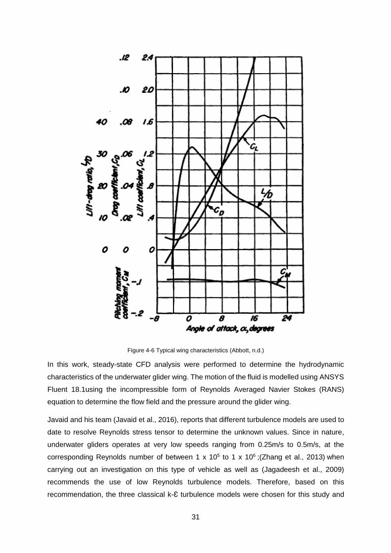
Figure 4-6 Typical wing characteristics (Abbott, n.d.)

In this work, steady-state CFD analysis were performed to determine the hydrodynamic

characteristics of the underwater glider wing. The motion of the fluid is modelled using ANSYS

Fluent 18.1using the incompressible form of Reynolds Averaged Navier Stokes (RANS)

equation to determine the flow field and the pressure around the glider wing.

Javaid and his team (Javaid et al., 2016), reports that different turbulence models are used to

date to resolve Reynolds stress tensor to determine the unknown values. Since in nature,

underwater gliders operates at very low speeds ranging from 0.25m/s to 0.5m/s, at the

corresponding Reynolds number of between 1 x 105 to 1 x 106 ;(Zhang et al., 2013) when

carrying out an investigation on this type of vehicle as well as (Jagadeesh et al., 2009)

recommends the use of low Reynolds turbulence models. Therefore, based on this

recommendation, the three classical k-Ԑ turbulence models were chosen for this study and

32

their predictions are compared to determine the one that yield reasonable result matching or

close to the published experimental data.

4.1.2.2 Turbulence resolution

According to (Javaid et al., 2016), underwater gliders operate within the speed range of

0.25m/s to 0.5 m/s, resulting in the Reynolds range of 1 x 105 to 1 x 106, which is classified as

low turbulence region. A steady-state analysis was employed to calculate the hydrodynamic

forces of the external flow on underwater glider wing. The selection of the CFD approach for

this study was compared with what is currently used by researchers and industrial partners

versus viable computational cost and for these reasons, Reynolds Averaged Navier-Stokes

(RANS) approach proved to be the most widely used and cost-effective approach. The RANS

turbulence models are divided into zero equation model, one equation model, two equations

and seven equation models. The study only focusses on the three k-epsilon two equation

models which solves turbulent kinetic energy equation k and turbulent dissipation ԑ. The three

k-epsilon models include Standard, Re-normalization group (RNG) and Realizable group and

their equations are discussed in detail in section 3.1.

The study investigated how the geometric design variations and operational parameters,

(AOA, speed and chord length) influence the hydrodynamic parameters (pressure, velocity,

drag coefficient, lift coefficient and pressure coefficient). Table 4.6 shows the ranges of the

speed and Reynolds numbers used in carrying out the study while the software-specific

settings are shown in table 4.5.

Table 4-4 Theoretical values of the flow quantities at different operating speeds and Reynolds range

1st 2nd 3rd 4th 5th 6th

Velocity(m/s) 0.1 0.26 0.28 0.3 0.4 0.5

Reynolds

number

10663.4

27725 29857.7 31990.3 42653.8

53317.2

The formula for calculating Reynolds number is given by equation 4.1 as:

𝑅𝑒 =𝜌𝑣𝐷ℎ

𝜇 (4.1)

Where 𝜌 is the density of the fluid,𝑣 velocity of the stream flow,𝐷ℎ hydraulic diameter of the

wing which is given by equation 4.2 and 𝜇 kinematic viscosity of the fluid.

33

𝐷ℎ =𝑎.𝑏

√𝑎2+𝑏2

2

(4.2)

Where 𝑎 is the thickness of the wing and 𝑏 is the chord length.

4.1.3 Numerical solution strategy and control

The convergence criterion is used to verify the accuracy of the numerical simulation by

monitoring the following parameters while computing the numerical solution: residual plots,

drag and lift coefficient s. The residual monitors satisfy convergence criterion when the

continuity, velocity (X, Y, Z), epsilon and k, drops below (1.0 x 10-4) as shown in figure 4.13

(Canonsburg, 2017). The number of iterations for running the simulation was set to at least

1000 iterations to ensure full convergence of the numerical results.

Figure 4-7 Convergence monitor using residuals curves

The solution control parameters such as the relaxation and under-relaxation control factors

shown in table 4.6 were used to control the stability of the numerical computations.

4.1.3.1 Solution parameters in fluent

The solution of the flow field representing incompressible fluid under steady state condition is

achieved by solving the Navier-Stokes equations using RANS approach. These equations are

discretized using finite volume approach. The solver settings implemented are double

34

Table 4-5 Control parameters -Relaxation and Under-Relaxation factors

Control Parameter Relaxation factors

Flow courant number 200

Momentum 0.5

Pressure 0.5

Control Parameter Under- Relaxation factors

Density 1

Body forces 1

Turbulent Kinetic energy 0.75

Turbulent dissipation rate 0.75

Turbulent viscosity 1

precision and pressure-based solver. Second order upwind scheme is used to approximate

the momentum equations, whilst the pressure-velocity coupling is realized through the couple

method. The boundary conditions and assumptions for correctly solving the physics of the

problem are discussed in section 4.6.1 and Table 6 gives a summary of the overall solution

approach.

4.1.3.2 BOUNDARY CONDITIONS

The boundary conditions for the computational domain are illustrated in figure 4.9. The flow

enters the computational domain from the upstream side with a free stream velocity of 0.26m/s

(Velocity -Inlet) and exit the computational domain downstream with atmospheric pressure

(pressure outlet). The flow is bounded by the walls (Ceiling, Bottom and back walls) with a

standard no-slip condition which implies that the velocity increases from zero at the wall

surface and to the free stream velocity away from the surface. To reduce the computational

load, a symmetry boundary condition is used at the symmetric plane where the conditions are

set to zero.

35

Table 4-6 Summary of the numerical simulation parameters in ANSYS Fluent

Settings Choice

Simulation type 3D Steady state Solver Double precision, Pressure based Temporal discretization Second order Turbulent model K-epsilon (RNG), Realizable and Standard Pressure -velocity coupling Couple Momentum 2nd order upwind Volume fraction 2nd order upwind Turbulent kinetic energy 2nd order upwind Turbulent dissipation rate 2nd order upwind Convergence criterion 1.0 x 10-4

4.1.3.3 Resolution of the near wall effect

In external flow simulation, the fluid behaviour away from the boundary layer can easily be

estimated due to its uniformity but closer to the wall, the fluid behaviour is unpredictable. Near

wall treatment is often employed in CFD to resolve the behaviour of the flow near an obstacle

or a wall. There are techniques implemented in this work to a certain degree to minimize the

CFD error due to the influence of this effect. For instance, inflation layers were used to capture

the turbulent effect around the wing and finer mesh around the wing was used to resolve the

finer details of the flow behaviour close to this surface. In addition, this study also employed

the built-in capability of the two equation turbulence models in ANSYS Fluent for handling the

near wall effects. These capabilities range from: Standard Wall Functions, Scalable Wall

Functions, Non-Equilibrium Wall Functions, Enhance Wall Treatment (EWT), Menter-Lechner

and User Defined Wall Functions.

Velocity Inlet Back wall Ceiling wall

Pressure outlet

Bottom Plane Symmetry Plane Wing Plane

Figure 4-8 Computational Domain boundary conditions

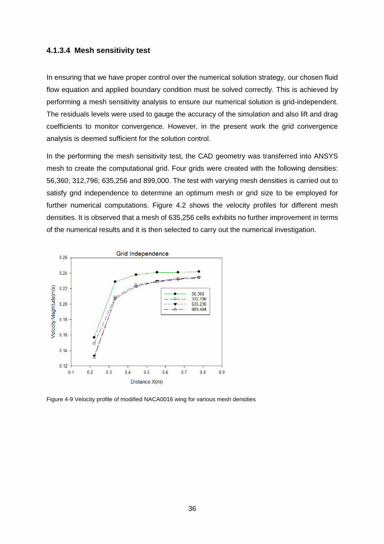
36

4.1.3.4 Mesh sensitivity test

In ensuring that we have proper control over the numerical solution strategy, our chosen fluid

flow equation and applied boundary condition must be solved correctly. This is achieved by

performing a mesh sensitivity analysis to ensure our numerical solution is grid-independent.

The residuals levels were used to gauge the accuracy of the simulation and also lift and drag

coefficients to monitor convergence. However, in the present work the grid convergence

analysis is deemed sufficient for the solution control.

In the performing the mesh sensitivity test, the CAD geometry was transferred into ANSYS

mesh to create the computational grid. Four grids were created with the following densities:

56,360; 312,796; 635,256 and 899,000. The test with varying mesh densities is carried out to

satisfy grid independence to determine an optimum mesh or grid size to be employed for

further numerical computations. Figure 4.2 shows the velocity profiles for different mesh

densities. It is observed that a mesh of 635,256 cells exhibits no further improvement in terms

of the numerical results and it is then selected to carry out the numerical investigation.

Figure 4-9 Velocity profile of modified NACA0016 wing for various mesh densities

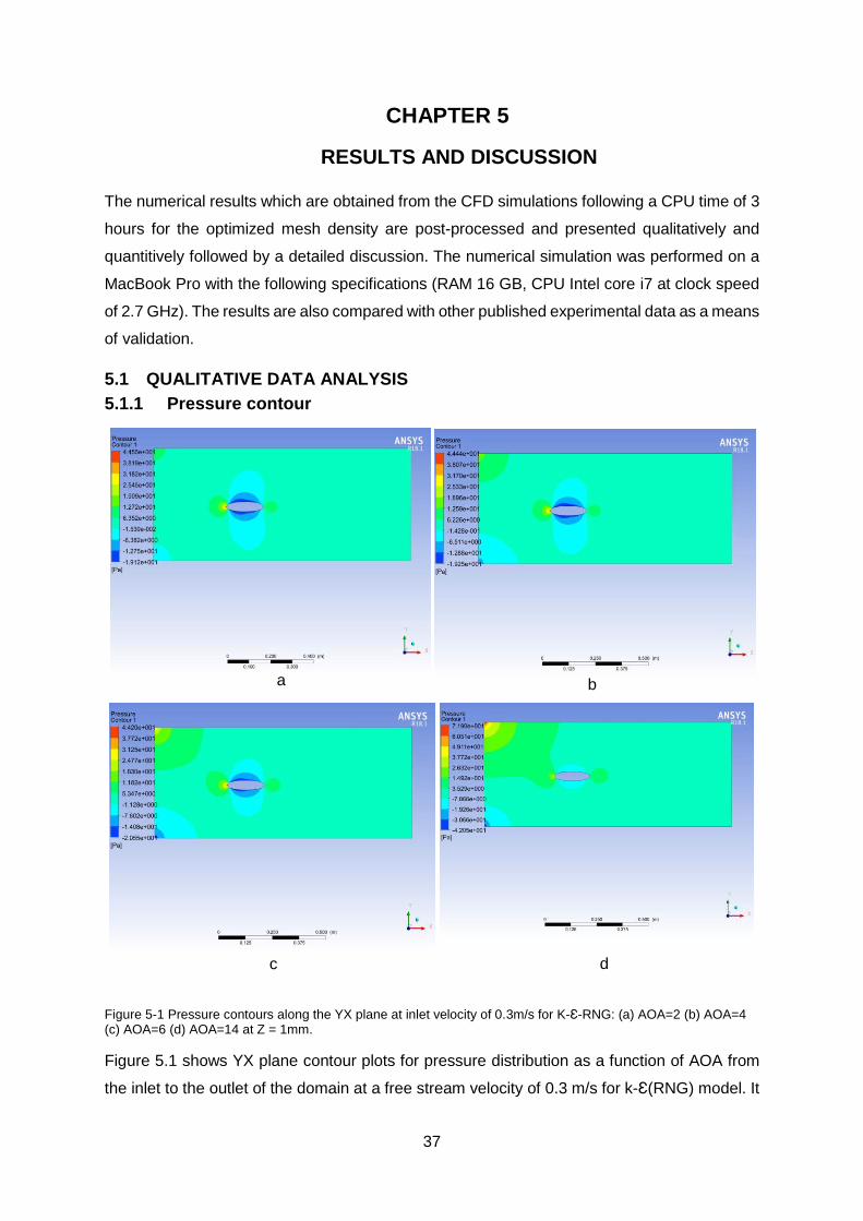
37

CHAPTER 5

RESULTS AND DISCUSSION

The numerical results which are obtained from the CFD simulations following a CPU time of 3

hours for the optimized mesh density are post-processed and presented qualitatively and

quantitively followed by a detailed discussion. The numerical simulation was performed on a

MacBook Pro with the following specifications (RAM 16 GB, CPU Intel core i7 at clock speed

of 2.7 GHz). The results are also compared with other published experimental data as a means

of validation.

5.1 QUALITATIVE DATA ANALYSIS

5.1.1 Pressure contour

Figure 5-1 Pressure contours along the YX plane at inlet velocity of 0.3m/s for K-Ԑ-RNG: (a) AOA=2 (b) AOA=4 (c) AOA=6 (d) AOA=14 at Z = 1mm.

Figure 5.1 shows YX plane contour plots for pressure distribution as a function of AOA from

the inlet to the outlet of the domain at a free stream velocity of 0.3 m/s for k-Ԑ(RNG) model. It

a b

c d

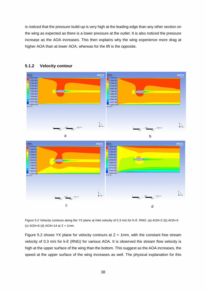
38

is noticed that the pressure build-up is very high at the leading edge than any other section on

the wing as expected as there is a lower pressure at the outlet. It is also noticed the pressure

increase as the AOA increases. This then explains why the wing experience more drag at

higher AOA than at lower AOA, whereas for the lift is the opposite.

5.1.2 Velocity contour

Figure 5-2 Velocity contours along the YX plane at inlet velocity of 0.3 m/s for K-Ԑ- RNG: (a) AOA=2 (b) AOA=4

(c) AOA=6 (d) AOA=14 at Z = 1mm.

Figure 5.2 shows YX plane for velocity contours at Z = 1mm, with the constant free stream

velocity of 0.3 m/s for k-Ԑ (RNG) for various AOA. It is observed the stream flow velocity is

high at the upper surface of the wing than the bottom. This suggest as the AOA increases, the

speed at the upper surface of the wing increases as well. The physical explanation for this

a b

c d

39

behaviour is the early separation of the fluid from the upper surface of the wing due to the

increasing AOA giving fluid less contact area hence an increase in speed.

5.1.3 Velocity vectors

Figure 5-3 Velocity vectors along the YX plane at inlet velocity of 0.3m/s for K-Ԑ-RNG: (a) AOA=2 (b) AOA=4 (c)

AOA=6 (d) AOA=14 at Z = 1mm.

Figure 5.3 shows velocity vector plots for various AOA, with a fixed velocity of 0.3 m/s for k-Ԑ

(RNG). It is noticed that the fluid flow around the wing of the underwater glider agrees with the

theoretical framework for external flow. As the AOA increases the fluid tends to follow the

trajectory path of the wing as depicted by the figures (a) to figure (d). Figure 5.3 also agrees

with figure 5.2 of the velocity contour as expected that the velocity increases with the AOA

and is higher at the upper surface of the wing.

(a) (b)

(c) (d)

40

5.1.4 Velocity streamlines

Figure 5-4 Velocity streamlines along the YX plane at inlet velocity of 0.3m/s for K-Ԑ-RNG: (a) AOA=2 (b)

AOA=4 (c) AOA=6 (d) AOA=14 at Z = 1mm.

Figure 5.4 shows the spatial representation of figure 5.3 and figure 5.2. The tracking of fluid

particle streamlines with massless particles give a clear fluid flow path from the free stream

inlet of the domain to the outlet in addition to depicting the variation of the flow velocities across

the lower surface and the upper surface of the wing. We can also observe from the flow stream

that the flow velocity magnitude shows a gradual decrease towards the pressure outlet.

(a) (b)

(c) (d)

41

5.2 QUANTITATIVE DATA ANALYSIS

The quantitative results of the spatial distribution of pressure, lift and drag coefficients along

the upper and lower surface of the glider wing, (close to the fuselage, at the centre of the span

and at the tip of the wing) are presented in the following sections. In comparing the influence

of the operating conditions on the hydrodynamic performance, the numerical data were

presented for different inlet velocities, angles of attack (AOA) and turbulence models. The

selected operating conditions are as follows: inlet velocities v= 0.1m/s, v = 0.26m/s, v=

0.28m/s, v= 0.3m/s, v =0.4 m/s and v= 0.5m/s, AOA starting from 2 to 14 degrees with the

increment of 2 degrees and k-Ԑ- Standard, k-Ԑ -RNG and k-Ԑ -Realizable models.

Figure 5-5 The 3D schematic view of the modified NACA0016 wing (a) is the point close to the fuselage of the

underwater glider at Z= 1mm (b) is the point at the centre of the wing span at Z = 150mm and (c) is the point at

the tip of the wing at Z= 300mm.

5.2.1 Surface distribution of the drag coefficient on the glider wing along the

chord length

x

y

z

42

5.2.1.1 Influence of the AOA and the free stream velocities on the drag

coefficient.

Figure 5-6 Drag coefficient as a function of the AOA (𝛼) (a) at different inlet velocities for K-Ԑ (RNG) (b) turbulent

models (c) AOAs

Figure 5.6 shows two sets of result namely: (a) CD as a function of the AOA, and (b) the

comparison of different turbulent models’ predictions of the drag coefficient as a function of

the AOA. It is observed that in figure (a) CD increases as the AOA increases yielding a similar

trend for different inlet velocities. This trend also suggest that CD is the function of speed. The

comparison of different inlet velocities showed the wing achieved more CD at lower velocities

than at the higher inlet velocities.(Abbott, n.d.)

(a)

a (degrees)

0 2 4 6 8 10 12 14 16

CD

0.00114

0.00116

0.00118

0.00120

0.00122

0.00124

0.00126

0.00128

0.00130

0.00132

0.00134

V= 0.26m/sV= 0.28m/sV= 0.3m/sV= 0.4m/s

a(degrees)

0 2 4 6 8 10 12 14 16

CD

0.00120

0.00125

0.00130

0.00135

0.00140

0.00145

0.00150

K-e (Std)

K-e(RNG)

K-e (Realizable)

(b)

43

In figure 5.6 (b) it is noticed that k-Ԑ (RNG) and k-Ԑ(Realizable) yielded almost similar results

compared to k-Ԑ (Standard). The results also suggest for this type of study k-Ԑ (Standard) is

not suitable.

5.2.2 Surface distribution of the lift coefficient on the glider wing

5.2.2.1 Influence of the aoa and the free stream velocities on the lift coefficient

Figure 5-7 Lift coefficient as a function of the AOA (a) inlet velocities (b) turbulence models (c) AOAs

Figure 5.7 shows two set of results namely: (a) CL as a function of the AOA, and (b) the

comparison of different turbulent models’ predictions of lift as a function of the AOA. The

(a)

a(degrees)

0 2 4 6 8 10 12 14 16

CL

4.0e-5

6.0e-5

8.0e-5

1.0e-4

1.2e-4

1.4e-4

1.6e-4

1.8e-4

2.0e-4

2.2e-4

2.4e-4

V= 0.26m/sV =0.28m/sV =0.3m/sV =0.4m/s

a(degrees)

0 2 4 6 8 10 12 14 16

CL

2e-5

4e-5

6e-5

8e-5

1e-4

1e-4

1e-4

2e-4

2e-4

2e-4

K-e (Std)

K-e(RNG)

K-e( Realizable)

(b)

44

results showed a similar trend for all inlet velocities, CL increases as the AOA increases until

reaches the maximum critical AOA after which it decreases. The critical AOA is defined as a

stall or where the glider has no further lift beyond this point. It is observed that the glider wing

reaches stalling point at approximately AOA =12 for all inlet velocities. Figure 5.7c also shows

that the coefficient of lift shows that it is the function of velocity However, at 0.3m/s the trend

shows some fluctuations which may be due to some level of solution instabilities occurring

during the simulation. This can be caused by many factors such, relaxing factors, courant

number etc.

Figure 5.7(b) shows the comparison of the three turbulent models and it is observed k-Ԑ (RNG)

and K-Ԑ (Realizable) yielded the same results coming to the same stalling point whereas for

k-Ԑ(Std) no distinct stalling point found. Therefore, it can be concluded for this type of work k-

Ԑ(Std) is not suitable. Mackenzie did an investigation on the flow around submarine using

three turbulent models, k-Ԑ (RNG), k-Ԑ (Realizable) and k-Ԑ(Standard), the results showed

the k-Ԑ(Std) performed badly in this application and was considered not suitable for this type

study which agrees with figure 5.7(b)

5.2.3 Surface distribution of the pressure coefficient on the glider wing along

the chord length on three YX Planes (symmetry, mid-point and wing tip)

along the span.

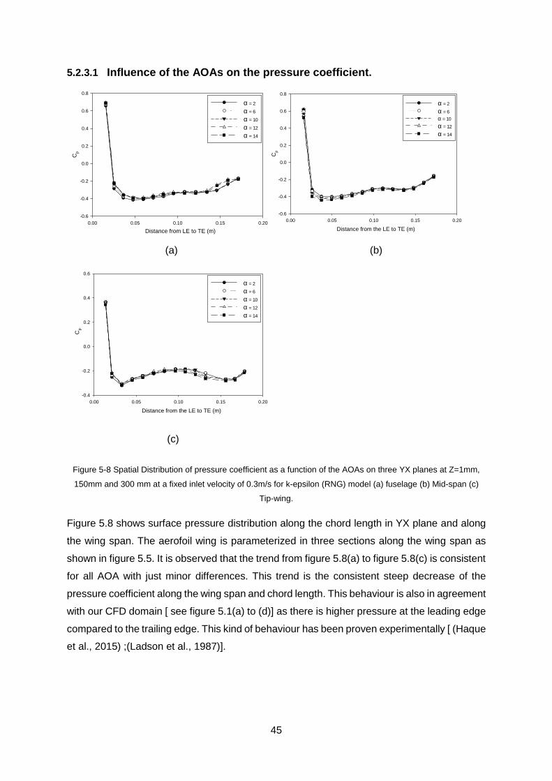
45

5.2.3.1 Influence of the AOAs on the pressure coefficient.

Figure 5-8 Spatial Distribution of pressure coefficient as a function of the AOAs on three YX planes at Z=1mm,

150mm and 300 mm at a fixed inlet velocity of 0.3m/s for k-epsilon (RNG) model (a) fuselage (b) Mid-span (c)

Tip-wing.

Figure 5.8 shows surface pressure distribution along the chord length in YX plane and along

the wing span. The aerofoil wing is parameterized in three sections along the wing span as

shown in figure 5.5. It is observed that the trend from figure 5.8(a) to figure 5.8(c) is consistent

for all AOA with just minor differences. This trend is the consistent steep decrease of the

pressure coefficient along the wing span and chord length. This behaviour is also in agreement

with our CFD domain [ see figure 5.1(a) to (d)] as there is higher pressure at the leading edge

compared to the trailing edge. This kind of behaviour has been proven experimentally [ (Haque

et al., 2015) ;(Ladson et al., 1987)].

(a) (b)

(c)

Distance from LE to TE (m)

0.00 0.05 0.10 0.15 0.20

Cp

-0.6

-0.4

-0.2

0.0

0.2

0.4

0.6

0.8

a = 2

a = 6

a = 10

a = 12

a = 14

Distance from the LE to TE (m)

0.00 0.05 0.10 0.15 0.20

Cp

-0.4

-0.2

0.0

0.2

0.4

0.6

a = 2

a = 6

a = 10

a = 12

a = 14

Distance from the LE to TE (m)

0.00 0.05 0.10 0.15 0.20

Cp

-0.6

-0.4

-0.2

0.0

0.2

0.4

0.6

0.8

a = 2

a = 6

a = 10

a = 12

a = 14

46

Table 5-1 Results summary of the influence of the AOA on Cp

Fuselage Mid-wing Tip-wing 𝜶 (degrees)

CpMax 0.69 0.65 0.38 2

CpMin -0.42 -0.41 -0.3

CpMax 0.7 0.6 0.38 6

CpMin -0.38 -0.41 -0.28

CpMax 0.72 0.58 0.37 10

CpMin -0.42 -0.41 -0.3

CpMax 0.72 0.55 0.37 12

CpMin -0.4 -41 -0.3

CpMax 0.72 0.53 0.36 14

CpMin -0.4 -0.48 -0.3

It also noteworthy that at the tip of the wing, the values of Cp irrespective of the change in the

AOA is relatively constant. The table also shows Cp at the fuselage is increasing with the AOA

whereas at mid-wing it is decreasing.

47

5.2.3.2 Influence of the inlet velocities on the pressure coefficient

Figure 5-9 Spatial Distribution of pressure coefficient as a function of inlet velocities on three YX planes at

Z=1mm, 150mm and 300 mm at a fixed AOA of 2 degrees for k-epsilon (RNG) model (a) fuselage (b) Mid span

(c) Tip.

The surface distribution of pressure coefficient at different inlet velocities along the chord

length in YX plane is presented in Figure 5.9. The wing is parameterized in the YX plane at

three different sections along the wing span (a) Z=1mm, (b) Z=150mm and (c) Z=300mm. It

is noticed that the spatial distribution of velocity along the chord length and along the span is

not uniform. It is also observed from figure 5.9 (a) for inlet velocities of 0.1m/s, 0.26 m/s, 0.3

m/s and 0.4 m/s, the maximum Cp is the same at 0.2, whereas at 0.28m/s, it reaches a

maximum Cp of 28.

Figure 5.9 (b) shows two distinct results whereby for the inlet speed of 0.1 m/s and 0.4 m/s

the maximum Cp is approximately 0.2, whereas for 0.26 m/s and 028 m/s shows the maximum

Cp of 23 and 26 respectively. Figure (c) also shows two similar distinct results, where for 0.1

m/s and 0.4 m/s the maximum Cp is 0.2 whilst 0.26m/s and 0.28m/s shows maximum Cp of 13

(a) (b)

(c)

2D Graph 1

Distance from LE to TE (m)

0.00 0.05 0.10 0.15 0.20

Cp

-20

-10

0

10

20

30

0.1 m/s0.26 m/s0.28 m/s0.3 m/s0.4 m/s

Distance from LE to TE (m)

0.00 0.05 0.10 0.15 0.20

Cp

-20

-10

0

10

20

30

0.1 m/s0.26 m/s0.28 m/s0.3 m/s0.4 m/s

2D Graph 3

Distance from LE to TE (m)

0.00 0.05 0.10 0.15 0.20

Cp

-15

-10

-5

0

5

10

15

20

0.1 m/s0.26 m/s0.28 m/s0.3 m/s0.4 m/s

48

and 15 respectively. The overall summation can be said that the Cp is higher closer to the

fuselage than at mid span and at the tip of the wing.

5.2.4 Hydrodynamic performance of the glider wing

5.2.4.1 Drag polar as a function of the AOA and the inlet velocities

Figure 5-10 The graph shows YX plane (a) Drag polar for different inlet speeds (CL vs CD) (b) CL/CD vs AOA (c)

CL/CD vs inlet velocities for k-Ԑ(RNG)

In optimizing the performance of the underwater glider wing, only the operating conditions

such as inlet velocity and AOA are considered. The influence of the geometric properties of

the aerofoil is not fully considered in this work as the aerofoil is of pre-defined form. Figure

5.10 (a) shows the drag polar performance at different AOA and different inlet velocities. The

figures show that inlet velocities have a significant impact on the CD and CL. It can also be

concluded that the minimal drag polar is around the inlet velocity of 0.26 m/s, which can be

selected as the optimal design point.

CD

0.00114 0.00116 0.00118 0.00120 0.00122 0.00124 0.00126

CL

4.0e-5

6.0e-5

8.0e-5

1.0e-4

1.2e-4

1.4e-4

1.6e-4

1.8e-4

2.0e-4

2.2e-4

2.4e-4

V= 0.26 m/sV= 0.28 m/sV = 0.3 m/sV= 0.4 m/s

(a) (b)

(c)

V (m/s)

0.0 0.1 0.2 0.3 0.4 0.5 0.6

CL/C

D

0.00

0.02

0.04

0.06

0.08

0.10

0.12

0.14

0.16

0.18

0.20

a = 2 a = 4 a = 6 a = 8 a = 10 a = 14a = 12

2D Graph 5

a (degrees)

0 2 4 6 8 10 12 14 16

CL/C

D

0.00

0.02

0.04

0.06

0.08

0.10

0.12

0.14

0.16

0.18

0.20

V = 0.1 m/sV = 0.26 m/sV = 0.28 m/sV = 0.3 m/sV = 0.4 m/sV = 0.5 m/s

49

Figure 5.10 (b) shows CL/CD ratio as the function of the AOA varies with inlet speeds. It is

noticed that for both figure 5.10 (b) and figure 5.7(a), the critical AOA of attack is approximately

12. Figure 5.10 (c) shows how CL/CD ratio as the function of speed varies with the different

AOAs. It can be seen form the chart that gradually increases with the inlet velocities with the

largest increase recorded at higher angles of attack.

5.2.5 Influence of the farfield boundary on the numerical results

It is well established that the farfield boundary conditions can affect the numerical predictions

of an aerofoil subjected to hydrodynamic force. However, the domain size in this study has

been carefully chosen to minimise this effect. Therefore, the effects of the farfield boundary

conditions on the numerical results has not been considered in this study.

50

CHAPTER 6

CONCLUSION

Underwater glider wings are the lifting surfaces with the chosen aerofoil sections. The

efficiency as well as the performance of an underwater glider mostly depends on the

hydrodynamic characteristics e.g. lift, drag, lift to drag ratio, etc on the wings. Besides many

factors, the effects of wing shape are also crucial to the design and underwater glider

performance. This study presents the numerical investigation to explore the hydrodynamic

performance improvement obtained by incorporating curvature at the trailing edge of a wing

as oppose to the standard straight or sharp trailing edge.

A CAD model with straight leading edge and trailing edge i.e. rectangular planform was

prepared with NACA 0016 using SolidWorks 2017. The operating conditions were setup such

that the inlet velocities varies from 0.1 m/s ,0.26 m/s ,0.28 m/s ,0.3 m/s ,0.4m/s and 0.5 m/s

corresponding to a Reynolds number of 27.8 x 103 and 53 x 103.The static pressure at

different angles of attack (AOA) ranging from 2 to 16 degrees at the increment of 2degrees for

three turbulent models i.e. k-Ԑ (standard), k-Ԑ (RNG) and k-Ԑ (Realizable) was calculated for

both upper and lower surfaces of the modified wing model using ANSYS Fluent 18.1.

Thereafter the static pressure distribution, lift coefficient, drag coefficient, lift to drag ratio and

pressure coefficient for both upper and lower surfaces were analysed and the following can

be concluded from this study:

The lift and drag coefficient are a function of the AOA and free stream velocities. If

these parameters change the performance of the underwater glider and its

hydrodynamic behaviour changes.

The underwater glider wing is optimized using the CL/CD ratio as function of the AOA

and inlet velocities. The investigation showed the optimal design point of the AOA of

12 degrees at the corresponding speed of 0.26m/s. This is also shown in figure 5.8 (a)

which shows the CL as the function of the AOA. The critical AOA matched with the

optimal design point of 12degrees.

It is also observed that Cp varies across the wing span. The results showed the Cp is

higher closer to the fuselage and decreases in the mid and at the tip of the wing. This

can mean the wing experience more stress close to the fuselage than the rest of the

wing span. This therefore explains why more structural rigidity must be provided in this

region of high stress (pressure force) concentration.

In the case of two equation models, the turbulence model with more accurate

predictions are the K-Ԑ(RNG) and K-Ԑ (Realizable) models.

51

The drag and lift curve corresponded to the typical wing characteristics of the published

experiment data irrespective of the fluid medium and operating conditions.

52

CHAPTER 7

BIBLIOGRAPHY

Abbott, B.I.R.A.H. THEORY OF Including a Summary of Airfoil Data.

Ahmed, S. 2013. 0012 Wing Flapped at Different Flap Angles with. , 13(4).

Anon. No Title.

Anon. Lifting-line theory class notes.

Anon. 1 . Fluid Dynamics Around Airfoils 2 . Governing Equations. : 1–10.

Anon. Module G: Turbulent Compressible / Incompressible Flow Over an Isolated Airfoil.

Arvin, I., Branch, K., Numbers, R., Arvin, I. & Toghraie, D. 2016. 3D Simulation of turbulent Flow over Three Different Airfoils in Different Reynolds Numbers 2 nd International Congress of Recent Advances in Engineering ICRAE2014 3D Simulation of turbulent Flow over Three Different Airfoils in Different. , (February 2014): 1–7.

Aeronautics, N. 1977. Aerodynamic of Wing-Body With Characteristics Configuration Advanced General Sections and simple flap systems.

Azim, R., Hasan, M.M. & Ali, M. 2015. Numerical investigation on the delay of boundary layer separation by suction for NACA 4412. Procedia Engineering, 105(Icte 2014): 329–334. http://dx.doi.org/10.1016/j.proeng.2015.05.013.

Barakos, G.N. & Drikakis, D. 2000. Unsteady separated flows over manoeuvring lifting surfaces. The Royal Society, 358: 3279–3291.

Battaglia, F. & Paul, M.R. 2014. 3D Dynamic Stall Simulation of Flow Over Naca0012 Airfoil At 10 5 and 10 6 Reynolds Numbers.

Bender, A., Steinberg, D.M., Friedman, A.L. & Williams, S.B. 2008. Analysis of an Autonomous Underwater Glider. Australasian Conference on Robotics and Automation 2008 (ACRA 08): 1–10. ftp://soest.hawaii.edu/bhowe/outgoing/For_Brian_S/Presentations/NavPapers-SWebster/bender-2008-usyd-glidermodel.pdf.

Bertram, V. 2012. Practical Ship Hydrodynamics. Practical Ship Hydrodynamics.

Bhatta, P. & Leonard, N.E. 2002. Stabilization and coordination of underwater gliders. Proceedings of the 41st IEEE Conference on Decision and Control, 2002., 2: 2081–2086. http://ieeexplore.ieee.org/lpdocs/epic03/wrapper.htm?arnumber=1184836.

Bhargava, V., Dwivedi, Y. & Rao, P. 2017. Analysis of Multi-Element Airfoil Configurations: A Numerical Approach. MOJ Applied Bionics and Biomechanics, 1(2): 7. http://medcraveonline.com.

Canonsburg, A.D. 2017. ANSYS Fluent User ’ s Guide. , (January).

Cimbala and Cengel. 2009. Fluid Dynamics.

Davis, R., Eriksen, C. & Jones, C. 2002. Autonomous buoyancy-driven underwater gliders. … Applications of Autonomous Underwater …: 1–11. http://www.ifremer.fr/lpo/gliders/donnees_tt/references/techno/4Gliders.pdf.

Diego, U.C.S., Scott, A. & Douglas, E. Scripps Institution of Oceanography.

53

Diab, H., Younes, R. & Lafon, P. 2017. Survey of research on the optimal design of sea harbours. International Journal of Naval Architecture and Ocean Engineering, 9(4): 460–472. http://dx.doi.org/10.1016/j.ijnaoe.2016.12.004.

Division, S. & Undersea, N. 2002. Maneuvering Hydrodynamics of Fish and Small Underwater Vehicles 1. , 117: 102–117.

Dod, D.C.P. 1946. LIMITATION CHANGES TO : FROM : NASA TR Server website.

Dwivedi, Y.D., Prasad, M.S. & Dwivedi, S. 2018. Experimental Aerodynamic Static Stability Analysis of Different Wing Planforms. , (April).

Executive, P. & Defence, M.O.F. PROCUREMENT EXECUTIVE , MINISTRY OF DEFENCE The Nature , Development and Effect of the Viscous an Aerofoil with Flow around High - Lift Devices. , (1258).

Fan, S. & Woolsey, C.A. 2014. Dynamics of underwater gliders in currents. Ocean Engineering, 84: 249–258. http://dx.doi.org/10.1016/j.oceaneng.2014.03.024.

Fulvio Bellobuono Tutor Coordinator Domenico Coiro Antonio Moccia, E.P. 2006. Aircraft Endurance Improvement Through Turbulent Separation Control. , (December).

Gómez, A. & Pinilla, Á. 2006. Aerodynamic Characteristics of Airfoils with Blunt Trailing Edge. Revista de Ingeniería, (24): 23–33. http://www.scielo.org.co/scielo.php?script=sci_arttext&pid=S0121-49932006000200004&lng=en&nrm=iso&tlng=en.

Gliders, A.U. 2008. Autonomous Underwater Gliders.

Haque, M.N., Ali, M. & Ara, I. 2015. Experimental investigation on the performance of NACA 4412 aerofoil with curved leading edge planform. Procedia Engineering, 105(Icte 2014): 232–240. http://dx.doi.org/10.1016/j.proeng.2015.05.099.

Hussain, N.A.A., Arshad, M.R. & Mohd-Mokhtar, R. 2011. Underwater glider modelling and analysis for net buoyancy, depth and pitch angle control. Ocean Engineering, 38(16): 1782–1791. http://dx.doi.org/10.1016/j.oceaneng.2011.09.001.

Ichihashi, N., Ikebuchi, T. & Arima, M. 2008. Development of an Underwater Glider with Independently Controllable Main Wings. Proceedings of the International Offshore and Polar Engineering Conference, 8: 156–161.

Isa, K. & Arshad, M.R. 2012. Buoyancy-driven underwater glider modelling and analysis of motion control. Indian Journal of Marine Sciences, 41(6): 516–526.

Jagadeesh, P., Murali, K. & Idichandy, V.G. 2009. Experimental investigation of hydrodynamic force coefficients over AUV hull form. Ocean Engineering, 36(1): 113–118.

Javaid, M.Y., Ovinis, M., Hashim, F.B.M., Maimun, A., Ahmed, Y.M. & Ullah, B. 2017. Effect of wing form on the hydrodynamic characteristics and dynamic stability of an underwater glider. International Journal of Naval Architecture and Ocean Engineering, 9(4): 382–389. http://dx.doi.org/10.1016/j.ijnaoe.2016.09.010.

Javaid, M.Y., Ovinis, M., Hashim, F.B.M., Maimun, A., Ahmed, Y.M. & Ullah, B. 2016. Effect of wing form on the hydrodynamic characteristics and dynamic stability of an underwater glider. International Journal of Naval Architecture and Ocean Engineering. http://linkinghub.elsevier.com/retrieve/pii/S2092678216304691.

Jeong, D.H., Roh, M. Il, Ham, S.H. & Lee, C.Y. 2017. Performance analyses of naval ships based on engineering level of simulation at the initial design stage. International Journal of Naval Architecture and Ocean Engineering, 9(4): 446–459.

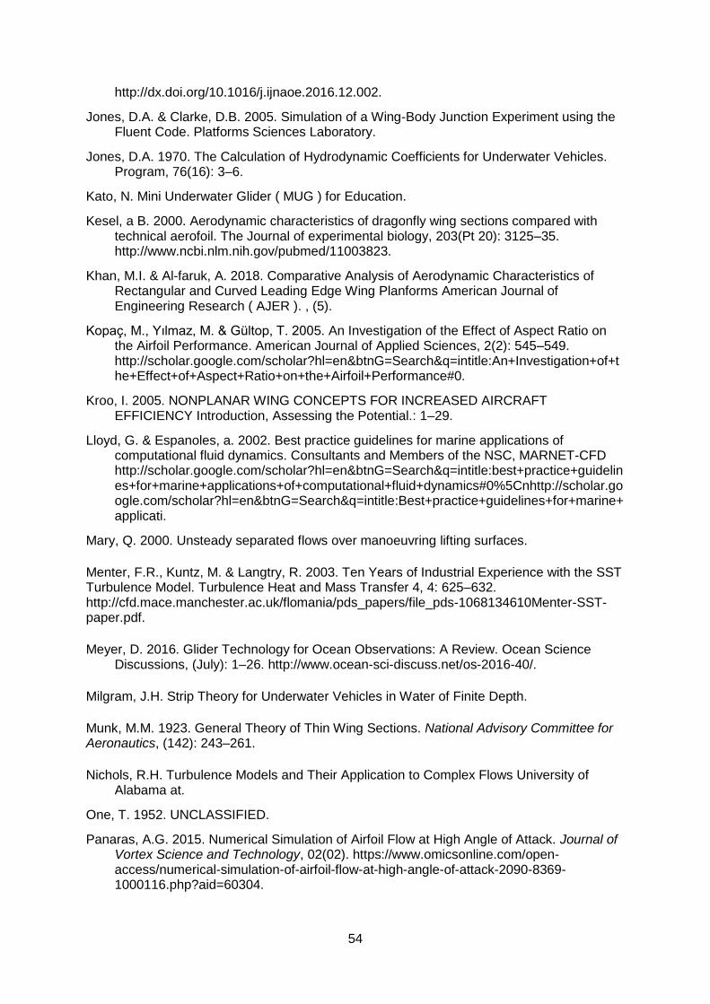
54

http://dx.doi.org/10.1016/j.ijnaoe.2016.12.002.

Jones, D.A. & Clarke, D.B. 2005. Simulation of a Wing-Body Junction Experiment using the Fluent Code. Platforms Sciences Laboratory.

Jones, D.A. 1970. The Calculation of Hydrodynamic Coefficients for Underwater Vehicles. Program, 76(16): 3–6.

Kato, N. Mini Underwater Glider ( MUG ) for Education.

Kesel, a B. 2000. Aerodynamic characteristics of dragonfly wing sections compared with technical aerofoil. The Journal of experimental biology, 203(Pt 20): 3125–35. http://www.ncbi.nlm.nih.gov/pubmed/11003823.

Khan, M.I. & Al-faruk, A. 2018. Comparative Analysis of Aerodynamic Characteristics of Rectangular and Curved Leading Edge Wing Planforms American Journal of Engineering Research ( AJER ). , (5).

Kopaç, M., Yılmaz, M. & Gültop, T. 2005. An Investigation of the Effect of Aspect Ratio on the Airfoil Performance. American Journal of Applied Sciences, 2(2): 545–549. http://scholar.google.com/scholar?hl=en&btnG=Search&q=intitle:An+Investigation+of+the+Effect+of+Aspect+Ratio+on+the+Airfoil+Performance#0.

Kroo, I. 2005. NONPLANAR WING CONCEPTS FOR INCREASED AIRCRAFT EFFICIENCY Introduction, Assessing the Potential.: 1–29.

Lloyd, G. & Espanoles, a. 2002. Best practice guidelines for marine applications of computational fluid dynamics. Consultants and Members of the NSC, MARNET-CFD http://scholar.google.com/scholar?hl=en&btnG=Search&q=intitle:best+practice+guidelines+for+marine+applications+of+computational+fluid+dynamics#0%5Cnhttp://scholar.google.com/scholar?hl=en&btnG=Search&q=intitle:Best+practice+guidelines+for+marine+applicati.

Mary, Q. 2000. Unsteady separated flows over manoeuvring lifting surfaces.

Menter, F.R., Kuntz, M. & Langtry, R. 2003. Ten Years of Industrial Experience with the SST Turbulence Model. Turbulence Heat and Mass Transfer 4, 4: 625–632. http://cfd.mace.manchester.ac.uk/flomania/pds_papers/file_pds-1068134610Menter-SST-paper.pdf.

Meyer, D. 2016. Glider Technology for Ocean Observations: A Review. Ocean Science Discussions, (July): 1–26. http://www.ocean-sci-discuss.net/os-2016-40/.

Milgram, J.H. Strip Theory for Underwater Vehicles in Water of Finite Depth.

Munk, M.M. 1923. General Theory of Thin Wing Sections. National Advisory Committee for Aeronautics, (142): 243–261.

Nichols, R.H. Turbulence Models and Their Application to Complex Flows University of Alabama at.

One, T. 1952. UNCLASSIFIED.

Panaras, A.G. 2015. Numerical Simulation of Airfoil Flow at High Angle of Attack. Journal of Vortex Science and Technology, 02(02). https://www.omicsonline.com/open-access/numerical-simulation-of-airfoil-flow-at-high-angle-of-attack-2090-8369-1000116.php?aid=60304.

55

Pneumatically, T.O.F.A., Underwater, P. & For, G. 2015. Design and Testing of a Pneumatically Propelled Underwater Glider for Shallow Water.

Rahimi, H., Medjroubi, W., Stoevesandt, B. & Peinke, J. 2014. 2D Numerical Investigation of the Laminar and Turbulent Flow Over Different Airfoils Using OpenFOAM. Journal of Physics: Conference Series, 555(1): 012070. http://stacks.iop.org/1742-6596/555/i=1/a=012070.

Raj, S. & Chandra, S. 2014. Advancement in autonomous underwater vehicles: Design &; performance perspective. 19th Offshore Symposium 2014: Emerging Technologies in Offshore Drilling and Production, (February): 374–380. https://www.scopus.com/inward/record.uri?eid=2-s2.0-84942163573&partnerID=40&md5=a7581caae16195fe2cad6f6db506302d.

Rudnick, D.L., Davis, R.E., Eriksen, C.C. & Fratantoni, D.M. Full-Text. : 48–59.

Riegels, F.W. 1961. Aerofoil Sections results from wind-tunnel investigations theoretical foundations.

Selig, M.S. 2003. Low Reynolds Number Airfoil Design Lecture Notes - Various Approaches to Airfoil Design. Low Reynolds Number Airfoil Design Lecture Notes - Various Approaches to Airfoil Design, (November): 24–28. http://www.ae.illinois.edu/m-selig/pubs/Selig-2003-VKI-LRN-Airfoil-Design-Lecture-Series.pdf.

Sherman, J., Davis, R.E., Owens, W.B. & Valdes, J. 2001. The autonomous underwater glider. Oceanic Engineering, IEEE Journal of, 26(4): 437–446.

Shi, Y., Pan, G., Jiang, J., Shi, Y. & Pan, G. 2013. Computation of Hydrodynamic Coefficients of Portable Autonomous Underwater Vehicle. : 2013.

Singh, Y., Bhattacharyya, S.K. & Idichandy, V.G. 2017. CFD approach to modelling, hydrodynamic analysis and motion characteristics of a laboratory underwater glider with experimental results. Journal of Ocean Engineering and Science, 2(2): 90–119. http://linkinghub.elsevier.com/retrieve/pii/S2468013316300729.

Stockdill, B., Pedro, G., Suleiman, A., Magagnato, F. & Djilali, N. 2006. Simulation of Unsteady Turbulent Flow Over a Stalled Airfoil. Computational Fluid Dynamics Journal, 14(4): 359–378.

Sun, C., Song, B. & Wang, P. 2015. Parametric geometric model and shape optimization of an underwater glider with blended-wing-body. International Journal of Naval Architecture and Ocean Engineering, 7(6): 995–1006. http://dx.doi.org/10.1515/ijnaoe-2015-0069.

Theodorsen, T. 1932. Theory of wing sections of arbitrary shape. NACA Report. http://www.pdas.com/refs/rep411.pdf.

Thomareisa, N. & Papadakis, G. 2017. Effect of trailing edge shape on the separated flow characteristics around an airfoil at low reynolds number: A numerical study. Physics of Fluids, 29(1).

Versteeg and Malasekera. 2007. Computational Fluid Dynamics.

van de Wal, H.J.B. 2010. Design of a Wing with Boundary Layer Suction. : 155.

Vols, F., Our, A. & Engineering, O. Numerical Simulations Techniques applied to Coastal and Oceanographic Engineering - Computational Fluid Dynamics (CFD). Direct: 1–6.

Wang, C. & Anvar, A. 2012. Modeling and Simulation of Motion of an Underwater Robot Glider for Shallow-water Ocean Applications. : 18–21.

56

Wang, H., Teo, C.J., Khoo, B.C. & Goh, C.J. 2013. Computational aerodynamics and flight stability of Wing-In-Ground (WIG) craft. Procedia Engineering, 67: 15–24. http://dx.doi.org/10.1016/j.proeng.2013.12.002.

Wiebe, J.P., Beausoleil, M., Zhang, G. & Cialacu, V. 2010. Journal of Steroid Biochemistry and Molecular Biology Opposing actions of the progesterone metabolites 118(1): 125–132.

Xie, Y., Yang, C., Wang, P., Peng, S., Fan, S. & Zhang, S. 2013. Improved Performance of an Underwater Glider with Passively Rotatable Wings. , (3): 0–4.

Y, T.O.N.C.C.X. & Hickman, A. 1943. National Advisory Committee for Aeronautics. Journal of Applied Physics, 14(8): 399. http://link.aip.org/link/JAPIAU/v14/i8/p399/s1&Agg=doi.

You, D. & Bromby, W. 2012. Large-Eddy Simulation of Unsteady Separation Over a Pitching Airfoil at High Reynolds Number. Seventh International Conference on Computational Fluid Dynamics (ICCFD7): 1–9.

Zalovcik, B.J.A., Wood, C., Memorial, L. & Field, L. Wartime report.

Zhang, S., Yu, J., Zhang, A. & Zhang, F. 2013. Spiraling motion of underwater gliders: Modeling, analysis, and experimental results. Ocean Engineering, 60: 1–13. http://dx.doi.org/10.1016/j.oceaneng.2012.12.023.

Zhang, F., Zhang, F. & Tan, X. 2012. Steady Spiraling Motion of Gliding Robotic Fish. : 1754–1759.

Zimmerman,C.H. 1932. Characteristics of Clark Y Airfoils of Small Aspect Ratios. National Advisory Committee for Aeronautics, Langley Memorial Aeronautical Laboratory: 581. http://naca.central.cranfield.ac.uk/reports/1933/naca-report-431.pdf.

57

APPENDICES

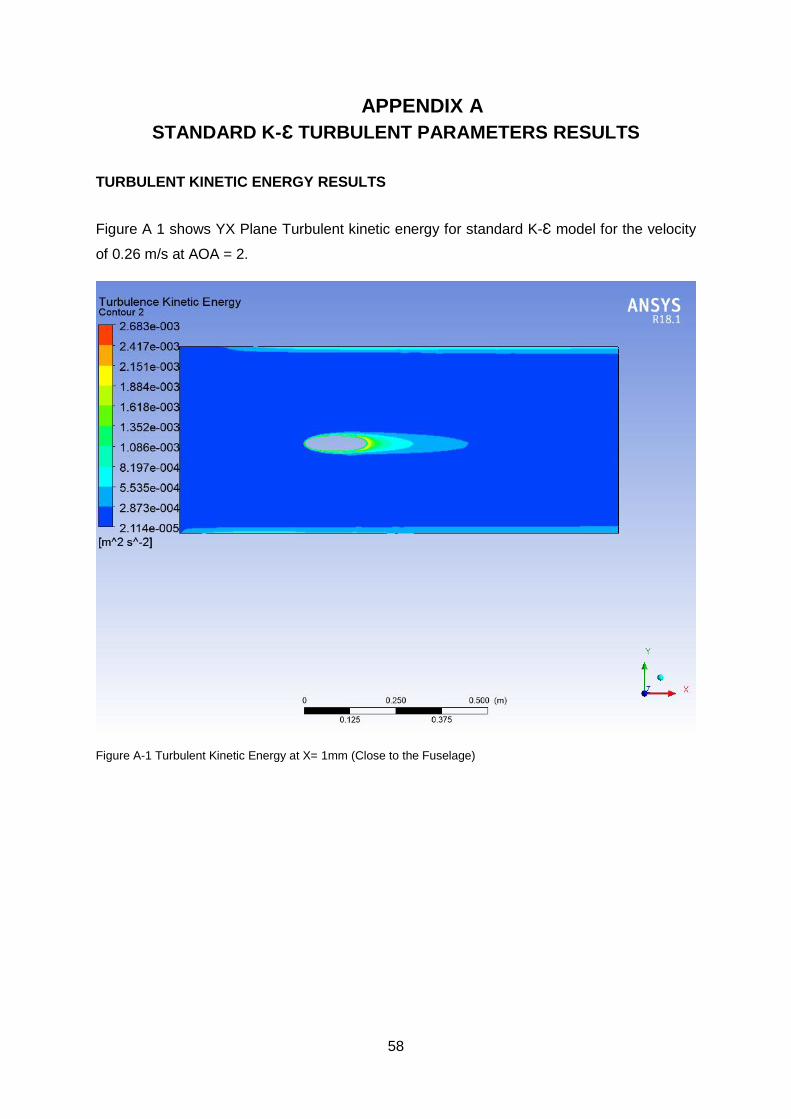
58

APPENDIX A

STANDARD K-Ԑ TURBULENT PARAMETERS RESULTS

TURBULENT KINETIC ENERGY RESULTS

Figure A 1 shows YX Plane Turbulent kinetic energy for standard K-Ԑ model for the velocity

of 0.26 m/s at AOA = 2.

Figure A-1 Turbulent Kinetic Energy at X= 1mm (Close to the Fuselage)

59

Figure A 2 shows YX Plane Turbulent kinetic energy for standard K-Ԑ model for the velocity

of 0.26 m/s at AOA = 2.

Figure A-2 Turbulent Kinetic Energy at X= 150 mm (Mid-Wing)

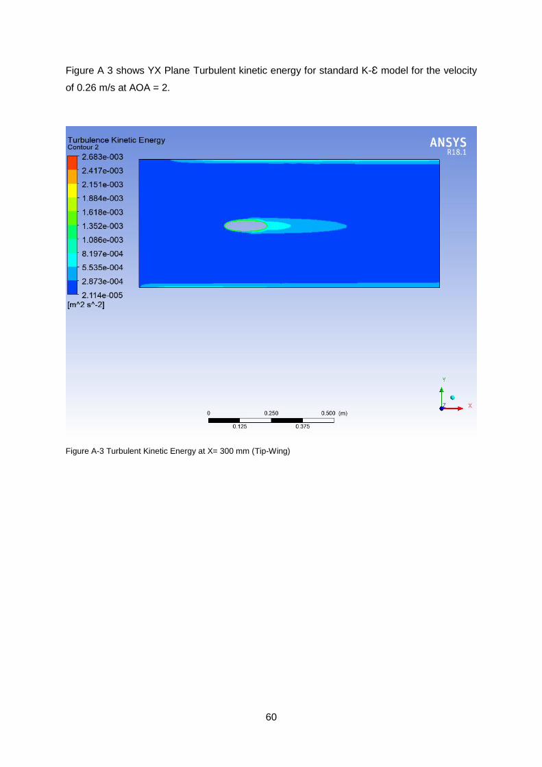
60

Figure A 3 shows YX Plane Turbulent kinetic energy for standard K-Ԑ model for the velocity

of 0.26 m/s at AOA = 2.

Figure A-3 Turbulent Kinetic Energy at X= 300 mm (Tip-Wing)

61

EDDY VISCOSITY RESULTS – K-Ԑ(Standard)

Figure A 4 shows YX Plane Eddy Viscosity for standard K-Ԑ model for the velocity of 0.26 m/s

at AOA = 2.

Figure A-4 Eddy Viscosity at X= 1mm (close to the fuselage)

62

Figure A 5 shows YX Plane Eddy Viscosity for standard K-Ԑ model for the velocity of 0.26 m/s

at AOA = 2.

Figure A-5 Eddy Viscosity at X= 150mm (Mid-Wing)

63

Figure A 6 shows YX Plane Eddy Viscosity for standard K-Ԑ model for the velocity of 0.26 m/s

at AOA = 2.

Figure A-6 Eddy Viscosity at X= 300mm (Tip-Wing)

64

APPENDIX B

STANDARD K-Ԑ(RNG) TURBULENT PARAMETERS RESULTS

TURBULENT KINETIC ENERGY RESULTS

Figure B1 shows YX Plane Turbulent Kinetic Energy for K-Ԑ -RNG model for the velocity of

0.26 m/s at AOA = 2.

Figure B-1 Turbulent Kinetic Energy at X= 1mm (Close to the fuselage)

65

Figure B2 shows YX Plane Turbulent Kinetic Energy for K-Ԑ -RNG model for the velocity of

0.26 m/s at AOA = 2.

Figure B-2 Turbulent Kinetic Energy at X= 150mm (Mid-Wing)

66

Figure B3 shows YX Plane Turbulent Kinetic Energy for K-Ԑ-RNG model for the velocity of

0.26 m/s at AOA = 2.

Figure B-3 Turbulent Kinetic Energy at X= 300mm (Tip-Wing)

67

EDDY VISCOSITY RESULTS - K-Ԑ (RNG)

Figure B4 shows YX Plane Eddy Viscosity for K-Ԑ-RNG model for the velocity of 0.26 m/s at

AOA = 2.

Figure B-4 Eddy Viscosity at X= 1mm (Close to the fuselage)

68

Figure B5 shows YX Plane Eddy Viscosity for K-Ԑ-RNG model for the velocity of 0.26 m/s at

AOA = 2.

Figure B-5 Eddy Viscosity at X= 150mm (Mid-Wing)

69

Figure B6 shows YX Plane Eddy Viscosity for K-Ԑ-RNG model for the velocity of 0.26 m/s at

AOA = 2.

Figure B-6 Eddy Viscosity at X= 300mm (Tip-Wing)

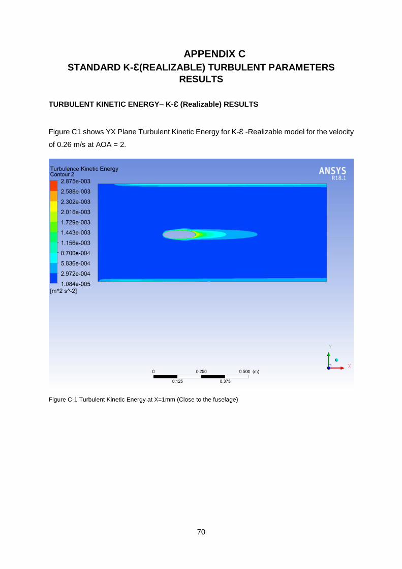
70

APPENDIX C

STANDARD K-Ԑ(REALIZABLE) TURBULENT PARAMETERS

RESULTS

TURBULENT KINETIC ENERGY– K-Ԑ (Realizable) RESULTS

Figure C1 shows YX Plane Turbulent Kinetic Energy for K-Ԑ -Realizable model for the velocity

of 0.26 m/s at AOA = 2.

Figure C-1 Turbulent Kinetic Energy at X=1mm (Close to the fuselage)

71

Figure C2 shows YX Plane Turbulent Kinetic Energy for K-Ԑ -Realizable model for the velocity

of 0.26 m/s at AOA = 2.

Figure C-2 Turbulent Kinetic Energy at X=150 mm (Mid-Wing)

72

Figure C3 shows YX Plane Turbulent Kinetic Energy for K-Ԑ -Realizable model for the velocity

of 0.26 m/s at AOA = 2.

Figure C-3 Turbulent Kinetic Energy at X=300 mm (Tip-Wing)

73

EDDY VISCOSITY RESULTS - K-Ԑ (Realizable)

Figure C4 shows YX Plane Eddy Viscosity for K-Ԑ -Realizable model for the velocity of 0.26

m/s at AOA = 2.

Figure C-4 Eddy Viscosity at X=1 mm (Close to the fuselage)

74

Figure C5 shows YX Plane Eddy Viscosity for K-Ԑ -Realizable model for the velocity of 0.26

m/s at AOA = 2.

Figure C-5 Eddy Viscosity at X=150 mm (Mid-Wing)

75

Figure C6 shows YX Plane Eddy Viscosity for K-Ԑ -Realizable model for the velocity of 0.26

m/s at AOA = 2.

Figure C-6 Eddy Viscosity at X=300 mm (Tip-Wing)