Embed Size (px)
Citation preview
TAUP-2292-15
FPAUO-15/03
New knotted solutions of Maxwell’s equations
Carlos Hoyos1, Nilanjan Sircar2 and Jacob Sonnenschein2
1Department of Physics, Universidad de Oviedo, Avda. Calvo Sotelo 18, 33007, Oviedo, Spain.
2Raymond and Beverly Sackler School of Physics and Astronomy, Tel-Aviv University, Tel-Aviv 69978, Israel.
[email protected], [email protected], and [email protected]
Abstract
In this note we have further developed the study of topologically non-trivial solutions
of vacuum electrodynamics. We have discovered a novel method of generating such solu-
tions by applying conformal transformations with complex parameters on known solutions
expressed in terms of Bateman’s variables. This has enabled us to get a wide class of so-
lutions from the basic configuration like constant electromagnetic fields and plane-waves.
We have introduced a covariant formulation of the Bateman’s construction and discussed
the conserved charges associated with the conformal group as well as a set of four types
of conserved helicities. We have also given a formulation in terms of quaternions. This
led to a simple map between the electromagnetic knotted and linked solutions into flat
connections of SU(2) gauge theory. We have computed the corresponding Chern-Simons
charge in a class of solutions and it takes integer values.
1
arX
iv:1
502.
0138
2v2
[he
p-th
] 3
May
201
5
Contents
1 Introduction 2
2 Bateman’s construction 4
2.1 Conserved charges . . . . . . . . . . . . . . . . . . . . . . . . . . . . . . . . . . 5
2.2 Examples . . . . . . . . . . . . . . . . . . . . . . . . . . . . . . . . . . . . . . . 7
3 Generating new solutions 9
3.1 Infinitesimal transformations of the solutions . . . . . . . . . . . . . . . . . . . . 11
3.2 (p,q)-knots from constant electric and magnetic field . . . . . . . . . . . . . . . 12
3.3 Knotted solutions from plane waves . . . . . . . . . . . . . . . . . . . . . . . . . 12
3.4 Complex deformations of Hopfions . . . . . . . . . . . . . . . . . . . . . . . . . . 14
4 Formal aspects of Bateman’s construction and knot solutions 19
4.1 Covariant formulation . . . . . . . . . . . . . . . . . . . . . . . . . . . . . . . . 20
4.2 Helicities . . . . . . . . . . . . . . . . . . . . . . . . . . . . . . . . . . . . . . . . 22
4.3 Quaternionic Formulation and Map to Non Abelian theories . . . . . . . . . . . 24
4.3.1 Winding number of non-Abelian solutions . . . . . . . . . . . . . . . . . 25
5 Summary 27
6 Acknowledgments 28
A Noether Charges 28
B θ, φ Formulation 30
B.1 Hopf index in 3-dimensions . . . . . . . . . . . . . . . . . . . . . . . . . . . . . . 30
B.2 (n,m)-link solutions in 3 + 1-dimension . . . . . . . . . . . . . . . . . . . . . . . 31
C Explicit expression of electric and magnetic field for Hopfion 33
1 Introduction
It is “common wisdom” that topological non-trivial solutions in field theory associate only with
non-linear equations of motion. That is the case for instance for two dimensional solitons,
magnetic monopoles and four dimensional Yang-Mills’ instantons. In fact it turns out that
this statement is false and there are also non-trivial configurations which solve linear equations
of motion. In particular there are known solutions of free Maxwell’s equations in flat space-
time that admit non-trivial topology, the Hopfion solution constructed in [3]. Since then there
have been considerable study of these solutions [4–7], which was recently revived in [8–12].
These solutions were studied as null electromagnetic solutions in Bateman’s [2] construction
in [13, 14]. The generalization and classification of analog solutions in higher spin fields was
studied in [15–18]. Linked and knotted non-null solutions of electrodynamics were studied
2
in [19]. A collection of comprehensive notes and references of such solutions in electrodynamics
and other areas of physics can be found in [20].
Since the original determination by Maxwell of the equations of motion of Electrodynam-
ics, many methods have been proposed to determine the evolution in space and time of the
electric and magnetic fields. The method we will use in this note is the so called Bateman’s
construction [2] which is based on grouping the electric and magnetic fields into a complex
vector field (Riemann-Silberstein vector [21, 25]), and expressing it in terms of two complex
functions α and β as follows,
F = E + iB F = ∇α×∇β. (1.1)
For this ansatz of the fields the solutions of the equations of motion are necessarily null namely
F2 = 0 ⇒ E2 −B2 = 0, E ·B = 0. (1.2)
Certain solutions of the equations of motion have a very cumbersome form when expressed
directly in terms of E and B but are very compact in terms of α and β. An example for that is
the remarkable solution which admits a non-trivial linking between the electric and magnetic
fields, which takes the form [14],
α =A− 1 + iz
A+ it, β =
(x− iy)
A+ it. (1.3)
where A = 12(x2 + y2 + z2 − t2 + 1). The solution has an implicit dependence on a scale
that we have set to one. We can make the dependence explicit by rescaling the coordinates
(t, x, y, z) −→ λ(t, x, y, z). Note also that the solution is valid for any conformally flat metric,
since Maxwell’s equations do not change. This space and time dependent solution has finite
energy, momentum, angular momentum, etc. The topological nature of this solution manifest
itself in the fact that it carries non-trivial “Chern-Simons (CS) helicity charges”. Exactly the
same charges are also characterizing the so called Hopfion solution of Maxwell’s equation [3], [4]
which can be derived from the basic Hopf map S3 → S2. It was shown in [13, 14] that in fact
there is an infinitely large family of solutions that can be derived from the basic one by mapping
α→ f(α, β) and β → g(α, β), where f and g are two arbitrary holomorphic functions. One may
wonder if there are other ways to easily generate new families of solutions, in this note we show
that the answer is in the affirmative. We will prove that any transformation associated with the
full conformal group SO(2, 4) but with complex rather than real parameters of a given solution
is also a solution of Maxwell’s equation. Obviously such transformations are not symmetries
of the Maxwell’s action however they do yield new solutions. Implementing this idea we found
out that applying a temporal special conformal transformation with an imaginary parameter
on a constant electric and magnetic perpendicular fields produces the topologically non-trivial
solution of (1.3). We further generated new solutions by applying such transformations on
plane waves and on the Hopfion (1.3) itself. One remarkable property of these transformations
is that they map solutions of infinite energy and Noether charges to solutions with finite energy
and charges.
3
We have discovered another interesting property of the knotted solutions of Maxwell’s equa-
tion. They can be mapped into SU(2) flat gauge connections. Defining a quaternionic valued
function
q =1√
|α|2 + |β|2(α + βj) (1.4)
We can map the unit quaternions to elements of SU(2) using a representation in terms of Pauli
matrices. Then, we write down a flat gauge connection as Qµ = q(∂µq∗). We determine the
winding number from the calculation of the non-Abelian Chern-Simons.
The paper is organized as follows. In the next section we review Bateman’s construction of
Maxwell’s equations. We write down the variables, the constraint equations and the method to
deduce from them the electric and magnetic fields. The conserved charges associated with the
conformal symmetry group that characterize the solutions are written down. We then describe,
using Bateman’s construction variables, three particular solutions: (i) Constant perpendicular
electric and magnetic fields, (ii) The plane wave solution, (iii) The Hopfion solution. The latter
is the basic prototype solution that admits non-trivial topology. In section 3 we describe the new
method for generating novel non-trivial solutions. The method utilizes transformations of the
full conformal group with complex rather than real parameters. We first prove that indeed the
transformed configurations are solutions of the equations of motion. We then show in section
3.2 how one can get the topologically non-trivial (p, q) solutions from a constant electric and
magnetic fields. Next we get knotted solutions from plane waves and in subsection 3.4 we
apply the complex transformation on the Hopfion configuration in particular time translations,
space translations, rotations, boosts, scalings and special conformal transformations. Section
4 is devoted to additional formal aspects of Bateman’s construction and knot solutions. In
subsection 4.1 we write down a covariant formulation of the construction and then in subsection
4.2 we derive general formulas for the helicities of the solutions. In section 4.3 we reformulate
Bateman’s construction using quaternionic fields. We show that this naturally leads to a relation
between the knotted Abelian solutions and flat SU(2) non-Abelian gauge connections with non-
zero winding number. Section 5 is devoted to a summary and a list of open questions. Three
appendices are added: In the first the Noether charges are determined, the second describes a
different formulation of the Hopfion solutions and in the third we write down explicit expressions
for the components of the electric and magnetic fields.
2 Bateman’s construction
A procedure to construct topologically non-trivial solutions in Maxwell’s equations is to use
Bateman’s construction [2]. In 3+1 dimensions we can group the electric and magnetic fields
in a single complex vector field, the Riemann-Silberstein vector [21,25]
F = E + iB. (2.1)
In the absence of charged matter, Maxwell’s equations for the complex field are
∇ · F = 0, i∂tF = ∇× F. (2.2)
4
We can satisfy the divergenceless condition with the general ansatz
F = ∇α×∇β, (2.3)
where α and β are complex. Then, the dynamical equation becomes
i∇× (∂tα∇β − ∂tβ∇α) = ∇× F. (2.4)
Which will be satisfied if
i(∂tα∇β − ∂tβ∇α) = F = ∇α×∇β. (2.5)
Solutions of this form have null norm
F2 = i(∂tα∇β − ∂tβ∇α) · (∇α×∇β) = 0 ⇒ E2 −B2 = 0, E ·B = 0. (2.6)
For this reason, they are also known as null solutions [13,14].
2.1 Conserved charges
We will characterize solutions by their conserved charges. In the first place we have the usual
conserved charges: energy E, momentum P and angular momentum L. They can be written
as integrals over space of the following gauge-invariant charge densities
• Energy density: E = 12(E2 + B2),
• Momentum density: p = (E×B),
• Angular momentum density: ` = (p× x).
Since Maxwell’s theory is invariant under conformal transformations, we have additional charge
densities associated to the following transformations 1
• Boosts: bv = (Ex−Pt),
• Dilatations: d = (p · x− Et),
• Temporal special conformal transformations (TSCT): k0 = ((x2 + t2)E − 2tp · x),
• Spatial special conformal transformations (SSCT): k = (2x(p · x)− 2tEx− (x2 − t2)p).
We will denote the conserved charges as Bv, D, K0 and K respectively.
For the null solutions we have an additional set of conserved charges that do not have a
gauge-invariant density, the electric and magnetic helicities. We define them as the integral
over space of the Chern-Simons form of the gauge potentials.
1The charge densities for special conformal transformation given here differ from that in [8], although their
value agree at t = 0. We provide a derivation of the right charges in Appendix A. We have explicitly checked
that they are time-independent.
5
Let us first define the complex vector potential V, such that F = ∇×V. We can decompose
it in real and imaginary parts V = C + iA, so it is clear that A is the usual gauge potential
and C is the ‘dual’ potential in the sense of electromagnetic duality
E = ∇×C, B = ∇×A. (2.7)
From Eq. (2.3), we can derive the relation between the gauge potentials and the functions α
and β. Up to gauge transformations
V = C + iA = α∇β. (2.8)
Then,
C = Re (α∇β), A = Im(α∇β). (2.9)
In this language, electromagnetic duality is simply the transformation α→ iα or β → iβ, which
clearly is a symmetry of the equations of motion (2.5).
The electric and magnetic helicities are defined as
hee =
∫d3xC · E, hmm =
∫d3xA ·B. (2.10)
They are gauge invariant when the integral is over all space, since ∇ · E = ∇ · B = 0. In
addition, we can define the cross helicities
hem =
∫d3xC ·B, hme =
∫d3xA · E. (2.11)
They are also gauge invariant when the integral is over all space.
To show that the helicities are conserved for the null solutions is very simple. For the
magnetic helicity we have
∂thmm =
∫d3x (∂tA ·B + A · ∂tB)
= −∫d3x ((E +∇Φ) ·B + A · (∇× E))
=
∫d3x (Φ∇ ·B− E · (∇×A)) = −
∫d3xE ·B = 0. (2.12)
We have used that E = −∂tA−∇Φ and E·B = 0 (A and φ are vector and scalar electromagnetic
potential). We can repeat the same calculation for the electric helicity hee using the dual
potential. For the cross helicities we can also show that they are conserved. For hme
∂thme =
∫d3x (∂tA · E + A · ∂tE)
=
∫d3x ((−E−∇Φ) · E + A · (∇×B))
=
∫d3x
(−E2 + Φ∇ · E + B · (∇×A)
)= −
∫d3x (E2 −B2) = 0. (2.13)
And a similar calculation can be done for hem.
6
In fact, for solutions found using Bateman’s construction, the two helicities have the same
value and the two cross helicities have opposite sign. One can show it using that the complex
potential is orthogonal to the complex field strength
V · F = α∇β · (∇α×∇β) = 0 ⇒ C · E−A ·B = 0, C ·B + A · E = 0. (2.14)
Therefore, all the solutions will have hee = hmm, hme = −hem.
2.2 Examples
There are several kind of known solutions to Maxwell’s equations that can be found using Bate-
man’s construction. The simplest solution one can consider is that corresponding to constant
electric and magnetic field,
α = 2i(t+ z)− 1 ; β = 2(x− iy). (2.15)
The corresponding electric and magnetic field are null and perpendicular to each other,
E = (−4, 0, 0); B = (0, 4, 0), (2.16)
This solution has diverging total energy and total helicity.
The next simplest are plane waves. An example is [14],
α = ei(z−t) ; β = x+ iy. (2.17)
Then,
F = (x+ iy)ei(z−t). (2.18)
This is a linearly polarized plane wave moving along the z direction. These solutions have finite
energy density and momentum, but all the charges diverge when integrated over the full space.
Therefore, we cannot associate well defined helicities to them.
A more interesting kind of solution is the Hopfion, that we describe in detail in the Ap-
pendix B.2. The Hopfion was originally found in [3], and the same solution was constructed
again later using Bateman’s construction in [14].2
α =A− 1 + iz
A+ it, (2.19)
β =(x− iy)
A+ it. (2.20)
where A = 12(x2 + y2 + z2 − t2 + 1). In this form, the functions α and β satisfy the additional
condition |α|2 + |β|2 = 1, so for fixed time they can be seen as the inverse of a stereographic
map of S3 to R3 ∪ {∞}. We use this later to give a general formula for the helicity that is
independent of the functional form of α and β. We must point out that although this is a nice
representation, it is not unique, in other representations |α|2 + |β|2 may not be a constant [14].
2This solution (field strength) is the same up to a trivial constant factor as that described in the Appendix B.2,
after the identification t→ −t and φ↔ θ.
7
The explicit form of the components of the electric and magnetic fields is given in appendix C
(similar expressions can also be found in the original work [4]. See also [18] for a review).
The Hopfion solution has finite energy E, momentum P = (0, 0,−E/2) and angular mo-
mentum L = (0, 0, E/2). It also has finite helicities hee = hmm = E/2. The Hopfion solution is
topologically non-trivial in the sense that electric and magnetic field lines are linked with each
other (Fig.(1b)).
The Hopfion solution was used in [14] to generate a large family of topologically non-trivial
solutions with different kinds of knots and links. The new solutions were found using the
following observation: each pair (α, β) in Bateman’s construction generates a whole family of
solutions by simply defining new functions (f, g) that depend holomorphically on α and β. The
new field strength is changed to
F = ∇f(α, β)×∇g(α, β) = h(α, β)∇α×∇β, (2.21)
i (∂tf∇g − ∂tg∇f) = h(α, β)i (∂tα∇β − ∂tβ∇α) . (2.22)
where h = ∂αf∂βg−∂βf∂αg. Clearly, if (α, β) satisfy the equations of motion, so do (f, g). The
new solutions have f = αp and g = βq. For co-prime integers (p, q) one finds various knots.
The (p, q)-knot solutions have finite energy E, that depends on the amplitude of the solutions.
The other charges are
• Momentum: P = (0, 0,− pp+q
E).
• Angular momentum: L = (0, 0, qp+q
E).
• Boosts: Bv = (0, 0, 0).
• Dilatations: D = 0.
• TSCT: K0 = E.
• SSCT: K = (0, 0,− pp+q
E)
• Helicities: hee = hmm = 1p+q
E.
• Cross helicities: hem = −hme = 0.
We can obtain the field lines corresponding to a vector field V i(xi) by solving for curves
given by xi(τ), where,dxi(τ)
dτ= V i(xi(τ)). (2.23)
This first order differential equation, along with the boundary condition xi(τ = 0) = xi0 gives
a field line passing through the point xi0. For the case of electric or magnetic lines, we use
normalized electric or magnetic field at a given time as V i. To check the periodicity of these
lines of force we can plot ln(|xi(τ) − xi(0)|) as a function of τ . For the Hopfion such a plot
is given in Fig.(1a). We also solve numerically field lines for the Hopfion and plot them in
Fig.(1b).
8
Alternatively, the structure of the solutions can be studied using surfaces that contain
electric and magnetic field lines and that we define below. For the (p, q) solutions with |α|2 +
|β|2 = 1, we can find a gradient field orthogonal to the electric and magnetic fields given by [14],
φ = φB + iφE = αpβq ; B · ∇φB = E · ∇φE = 0. (2.24)
So we can visualize the geometrical properties of these solutions by plotting the isosurfaces of
φE and φB, which contain the electric and magnetic field lines. Figs. (1c) and (1d) shows such
isosurfaces for the Hopfion. Properties of these isosurfaces were studied in detail in [14].
3 Generating new solutions
There are multiple possibilities to generate new solutions. One way that we have already
explained is to substitute α and β in Bateman’s construction by holomorphic functions of the
same solutions, with arbitrary complex coefficients. Another way is to use the symmetries of
the equations to produce new solutions. Clearly if we do a Poincare transformation we will
trivially obtain a new solution. Translations will not affect to the charges of the solutions,
while rotations will rotate momentum and angular momentum and boosts will also change the
energy and conformal charges. However, we do not see them as truly new solutions, since we
can recover the original form of the solution by simply changing the frame of reference.
A more interesting possibility is to consider other kind of deformations, such as scaling and
squeezing, or conformal transformations [28]. This is used sometimes in a different context in
order to check the stability of soliton solutions (see e.g. [32,33]). In general not all transforma-
tions will lead to a new solution, in order for this to happen it is necessary that the equations of
motion are on-shell invariant. In the case of Bateman’s construction there is a new interesting
generalization. Since the equations are complex, the deformations can also be made complex3.
In practice this could be interpreted as mixing usual deformations with electromagnetic duality,
that as we have seen corresponds to introducing imaginary factors in the solutions.
We will first use infinitesimal transformations to learn which ones can be used to generate
new solutions. Then, we will do finite transformations of the solutions and study their proper-
ties. In all cases we have checked explicitly that the equations of motion are satisfied by the
new deformed solutions. Although these complex transformations on the solutions generate
“new” solutions to the equations of motion, they might be sometimes related to each other by
a real transformation, and thus be in the same class.
For convenience we will use components rather than vectorial notation. Greek indices
µ, ν = 0, 1, 2, 3 refer to spacetime directions and Latin indices i, j = 1, 2, 3 refer to spatial
directions. For a spatial vector the curl and the divergence are
(∇×A)i = εijk∂jAk, (∇ ·A) = ∂iAi. (3.1)
For four-vectors we will raise and lower indices with the mostly plus metric ηµν = diag (−1, 1, 1, 1)
and define the epsilon tensor with spacetime indices as ε0ijk = −εijk.3It was pointed out to us (after appearance of our preprint in arXiv) that, previously complex transformation
of Maxwell solutions was studied in [22–25]. See also [26,27].
9

2 4 6 8 10Τ
-15
-10
- 5
lnH È xiH ΤL - xiH 0L ÈL
(a)
-1
0
1
2
x- 2
-1
0
1
y
-1
0
1
z
(b)
(c) (d)
Figure 1: Structure of Hopfion Solution. Fig(1a): Plot showing periodicity of field lines -
electric (Black), magnetic (Red) (which are overlapping in the figure). Fig.(1b): Shows electric
field line (in Black) and magnetic field line (in Red) at t = 0. Fig.(1c):Plot of surfaces φE = .45
(Red) and φB = .45 (Blue) at t = 0. Fig.(1d):Plot of surfaces φB = .4 (Red) and φB = .45
(Blue) at t = 0
10
3.1 Infinitesimal transformations of the solutions
Under an infinitesimal (complex) coordinate transformation xµ → xµ + ξµ, the functions α and
β change as
δα = ξλ∂λα, δβ = ξλ∂λβ. (3.2)
The equation of motion is
i(∂0α∂iβ − ∂iα∂0β)− εijk∂jα∂kβ = 0. (3.3)
Under the infinitesimal transformation there is a part ∼ ξλ∂λ(equation) which vanishes trivially
on-shell, and then there are the contributions
0 = i∂0ξλ(∂λα∂
iβ − ∂iα∂λβ) + i∂iξλ(∂0α∂λβ − ∂λα∂0β)− ∂jξλεijk(∂λα∂kβ − ∂kα∂λβ). (3.4)
We can write each term as follows using the equations of motion
i∂0ξλ(∂λα∂
iβ − ∂iα∂λβ) =(∂0ξ
0δil + i∂0ξnε iln
)εljk∂jα∂kβ,
i∂iξλ(∂0α∂λβ − ∂λα∂0β) = ∂iξlε jkl ∂jα∂kβ,
∂jξλεijk(∂λα∂kβ − ∂kα∂λβ) =
(i∂nξ
0ε nil − ∂lξi + ∂nξnδil)εljk∂jα∂kβ. (3.5)
All together, we find the condition
0 =[(∂0ξ
0 − ∂nξn)δil + i(∂0ξn − ∂nξ0)εlni + ∂iξl + ∂lξi
]ε jkl ∂jα∂kβ. (3.6)
It is immediate to see that this is satisfied for translations in all coordinates ξµ = cµ, Lorentz
transformations ξµ = Λµνx
ν , with Λµν = −Λνµ and dilatations ξµ = λxµ.
Let us write the derivative in the general form
∂iξj =1
3δij∂nξ
n +1
2σij +
1
2ωij, (3.7)
where ωij is the antisymmetric part and σij is symmetric and traceless. Then,
0 =
[(∂0ξ
0 − 1
3∂nξ
n
)δil + i(∂0ξ
n − ∂nξ0)εlni + σil]ε jkl ∂jα∂kβ. (3.8)
We see that the following conditions should be satisfied in general:
σij = 0, ∂0ξ0 − 1
3∂nξ
n = 0, ∂0ξn − ∂nξ0 = 0. (3.9)
Note that these conditions are also satisfied by special conformal transformations
ξµ = aµx2 − 2aλxλxµ. (3.10)
So new solutions can be generated by using conformal transformations with complex parame-
ters. Shear deformations on the other hand do not produce new solutions.
11
3.2 (p,q)-knots from constant electric and magnetic field
As a very simple application of complex deformations let us show how the Hopfion solution
or (1,1)-knot can be obtained through a conformal transformation of a solution with constant
electric and magnetic fields.
Let us choose the solution with constant field strength as given in (2.15),
α = 2i(t+ z)− 1 ; β = 2(x− iy) (3.11)
The corresponding electric and magnetic field are constant and have diverging total energy and
helicity. Now let us consider a special conformal transformation (SCT),
xµ → xµ − bµxσxσ
1− 2bσxσ + bσbσxρxρ. (3.12)
With the choice of the parameter, bµ = i(1, 0, 0, 0) the new (α, β) obtained by this transfor-
mation is the same as the Hopfion solution given by (2.19) and (2.20) 4. If we consider more
general choice of the parameter bµ, we can generate linked solution with various values of the
conserved charges.
Other knotted solutions can be generated by considering integer powers of (α, β) given in
(2.15), i.e. (α, β) → (αp, βq), and then considering a SCT with parameter bµ = i(1, 0, 0, 0).
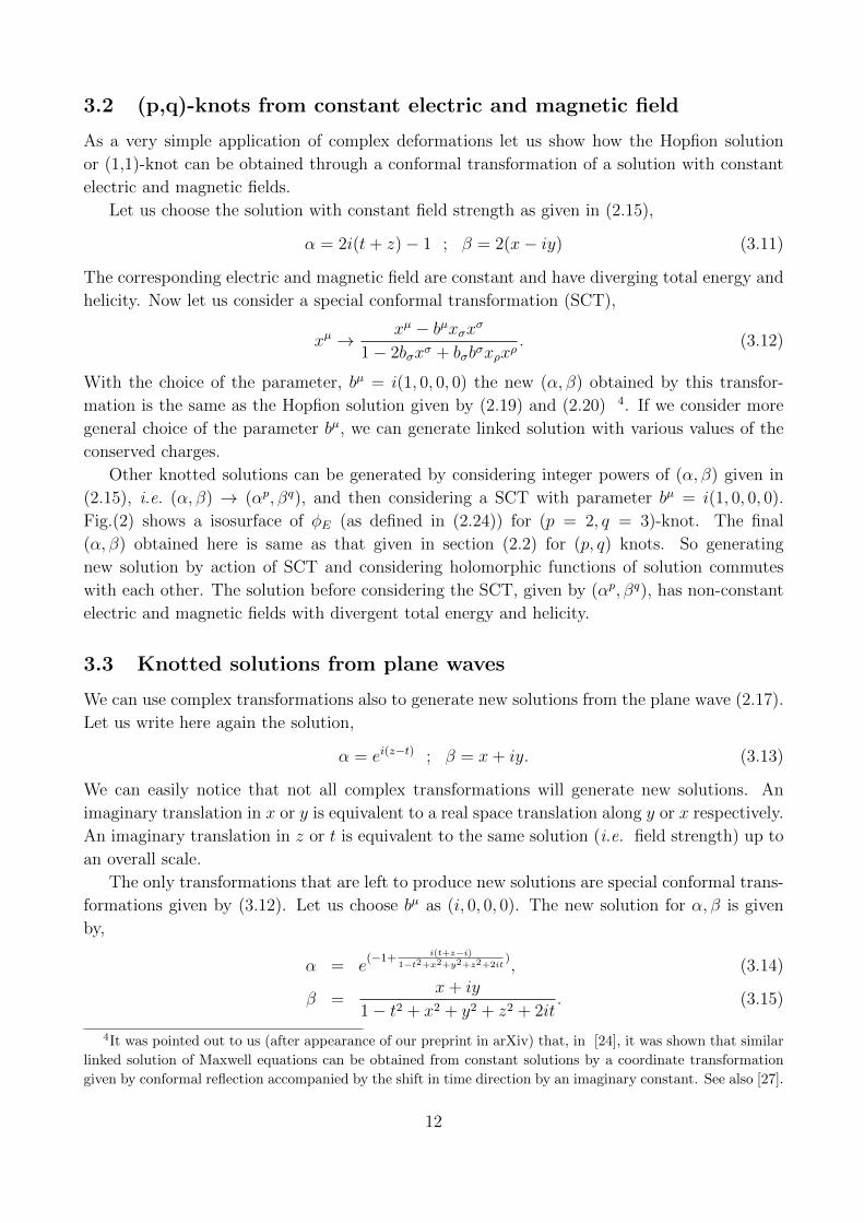
Fig.(2) shows a isosurface of φE (as defined in (2.24)) for (p = 2, q = 3)-knot. The final
(α, β) obtained here is same as that given in section (2.2) for (p, q) knots. So generating
new solution by action of SCT and considering holomorphic functions of solution commutes
with each other. The solution before considering the SCT, given by (αp, βq), has non-constant
electric and magnetic fields with divergent total energy and helicity.
3.3 Knotted solutions from plane waves
We can use complex transformations also to generate new solutions from the plane wave (2.17).
Let us write here again the solution,
α = ei(z−t) ; β = x+ iy. (3.13)
We can easily notice that not all complex transformations will generate new solutions. An
imaginary translation in x or y is equivalent to a real space translation along y or x respectively.
An imaginary translation in z or t is equivalent to the same solution (i.e. field strength) up to
an overall scale.
The only transformations that are left to produce new solutions are special conformal trans-
formations given by (3.12). Let us choose bµ as (i, 0, 0, 0). The new solution for α, β is given
by,
α = e(−1+
i(t+z−i)
1−t2+x2+y2+z2+2it), (3.14)
β =x+ iy
1− t2 + x2 + y2 + z2 + 2it. (3.15)
4It was pointed out to us (after appearance of our preprint in arXiv) that, in [24], it was shown that similar
linked solution of Maxwell equations can be obtained from constant solutions by a coordinate transformation
given by conformal reflection accompanied by the shift in time direction by an imaginary constant. See also [27].
12
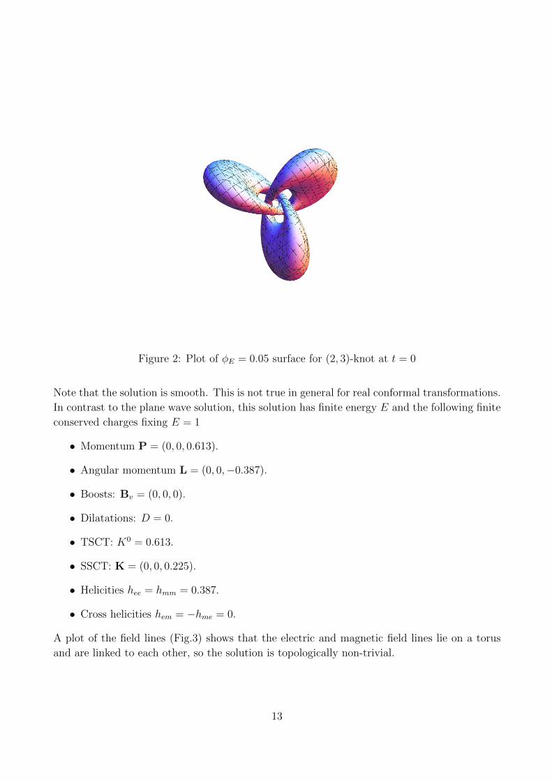
Figure 2: Plot of φE = 0.05 surface for (2, 3)-knot at t = 0
Note that the solution is smooth. This is not true in general for real conformal transformations.
In contrast to the plane wave solution, this solution has finite energy E and the following finite
conserved charges fixing E = 1
• Momentum P = (0, 0, 0.613).
• Angular momentum L = (0, 0,−0.387).
• Boosts: Bv = (0, 0, 0).
• Dilatations: D = 0.
• TSCT: K0 = 0.613.
• SSCT: K = (0, 0, 0.225).
• Helicities hee = hmm = 0.387.
• Cross helicities hem = −hme = 0.
A plot of the field lines (Fig.3) shows that the electric and magnetic field lines lie on a torus
and are linked to each other, so the solution is topologically non-trivial.
13
200 400 600 800Τ
-10
- 8
- 6
- 4
- 2
lnH È xiH ΤL - xiH 0L ÈL
(a) (b) (c)
Figure 3: Knotted Solutions from Plane Waves. Fig(3a): Plot showing periodicity of field
lines - electric (Black), magnetic (Red). Fig.(3b): Shows an electric field line (in Black) and a
magnetic field line (in Red) at t = 0. Fig.(3c): Shows two electric field lines at t = 0
3.4 Complex deformations of Hopfions
For the Hopfions we find that all complex transformations lead to new solutions. We list the
form of the new solutions and the conserved charges below:
• Time translation:
The solutions generated by the imaginary time translation t → t + ic, with c a constant
real parameter are,
α = N1A− 1 + iz
A+ i(t+ ic), (3.16)
β = N1(x− iy)
A+ i(t+ ic). (3.17)
where A = 12(x2 + y2 + z2 − (t + ic)2 + 1). We introduce a factor N1 as the overall
normalization, which is related to the energy E as N41 = E|1−c|5
2π2 .
The conserved charges for this solution are
– Momentum: P = (0, 0,−E2
).
– Angular momentum: L = (0, 0, 1−c2E).
– Boosts: Bv = (0, 0, 0).
– Dilatations: D = 0.
– TSCT: K0 = (1− c)2E.
– SSCT: K = (0, 0,−12(1− c)2E).
– Helicities: hee = hmm = 1−c2E.
14
– Cross helicities : hem = −hme = 0
The helicity in units of energy is a continuous function of the parameter c, but the
structure of electric and magnetic lines are same as that of Hopfion for all values of c 6= 1.
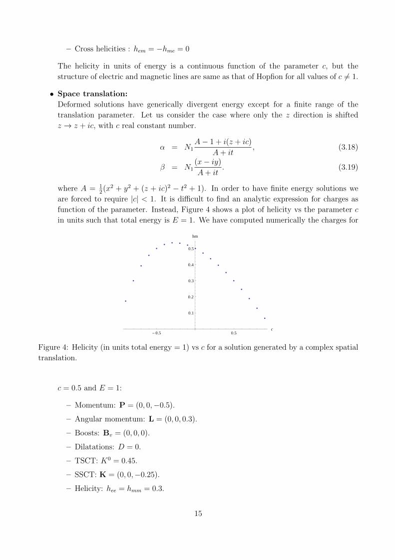
• Space translation:
Deformed solutions have generically divergent energy except for a finite range of the
translation parameter. Let us consider the case where only the z direction is shifted
z → z + ic, with c real constant number.
α = N1A− 1 + i(z + ic)
A+ it, (3.18)
β = N1(x− iy)
A+ it. (3.19)
where A = 12(x2 + y2 + (z + ic)2 − t2 + 1). In order to have finite energy solutions we
are forced to require |c| < 1. It is difficult to find an analytic expression for charges as
function of the parameter. Instead, Figure 4 shows a plot of helicity vs the parameter c
in units such that total energy is E = 1. We have computed numerically the charges for
-0.5 0.5 c
0.1
0.2
0.3
0.4
0.5
hm
Figure 4: Helicity (in units total energy = 1) vs c for a solution generated by a complex spatial
translation.
c = 0.5 and E = 1:
– Momentum: P = (0, 0,−0.5).
– Angular momentum: L = (0, 0, 0.3).
– Boosts: Bv = (0, 0, 0).
– Dilatations: D = 0.
– TSCT: K0 = 0.45.
– SSCT: K = (0, 0,−0.25).
– Helicity: hee = hmm = 0.3.
15
– Cross helicities : hem = −hme = 0
• Rotations:
We can also generate new solutions using rotations along the spatial coordinates with
complex angles. Rotations in the x, y plane by a complex angle amount to a rescaling of
the solution, thus they do not generate really new solutions. Non-trivial transformations
involve the z direction. Let us consider the following transformation in the x, z plane,
x → x cos(iθ) − z sin(iθ), z → z cos(iθ) + x sin(iθ). The new solution produced by this
transformation is,
α = N1A− 1 + i(z cos(iθ) + x sin(iθ))
A+ it, (3.20)
β = N1(x cos(iθ)− z sin(iθ)− iy)
A+ it. (3.21)
where A = 12(x2 + y2 + z2 − t2 + 1). The normalizationN1 is related to the energy E as
N41 = E
2π2 cosh2(θ). The charges for these solutions are
– Momentum: P = (0, 12
tanh(θ),−12sech(θ))E.
– Angular momentum: L = (0,−12
tanh(θ), 12sech(θ))E.
– Boosts: Bv = (0, 0, 0).
– Dilatations: D = 0.
– TSCT: K0 = E
– SSCT: K = (0, 12
tanh(θ),−12sech(θ))E.
– Helicities: hee = hmm = E/2.
– Cross helicities : hem = −hme = 0
In this case the helicity in units of the energy does not change.
• Boosts:
An imaginary boost along xi direction is given by,
t → t cosh(iθ)− xi sinh(iθ), (3.22)
xi → xi cosh(iθ)− t sinh(iθ), (3.23)
where θ is real. The expression of α, β for Hopfions is rotationally symmetric in the (x, y)
plane, so let us consider imaginary boosts along x and z here. We also introduce an overall
normalization N1 as before, related to the energy E as N41 = E
2π2 | cos θ|5, independently
of the direction of the boost.
The charges for the solution generated by boost along x direction (of energy E),
– Momentum: P = (0, E2
sin θ,−E2
cos θ).
– Angular momentum: L = (0, 0, 12E).
16
– Boosts: Bv = (− sin θE, 0, 0).
– Dilatations: D = 0.
– TSCT: K0 = E.
– SSCT: K = (0,−12
sin θE,−12
cos θE).
– Helicities: hee = hmm = 12
cos θE.
– Cross helicities: hem = −hme = 0.
The charges for a solution generated by boost along z (of energy E) are
– Momentum: P = (0, 0,−E2
).
– Angular momentum: L = (0, 0, 12
cos θE).
– Boosts: Bv = (0, 0,− sin θE).
– Dilatations: D = 12
sin θE.
– TSCT: K0 = E.
– SSCT: K = (0, 0,−12E).
– Helicities: hee = hmm = 12
cos θE.
– Cross helicities: hem = −hme = 0.
• Scaling:
Complex scalings xµ → bxµ generate new solutions, but if b is purely imaginary the energy
of the new solutions is always infinite and the helicity is zero. Instead is better to consider
transformations with b = 1 + ic, where c is real. Such solutions have finite and non-zero
energy and helicity for a finite range of the parameter c. For these solutions it is difficult
to get the analytic expression of the charges as function of c, but we can easily obtain
numerical results. For c = 1 and E = 1 we find the following values:
– Momentum: P = (0, 0,−0.5).
– Angular momentum: L = (0, 0, 0.25).
– Boosts: Bv = (0, 0, 0.25).
– Dilatations: D = −0.5.
– TSCT: K0 = 0.5
– SSCT: K = (0, 0,−0.25).
– Helicities: hee = hmm = 0.25.
– Cross helicities: hem = −hme = 0.
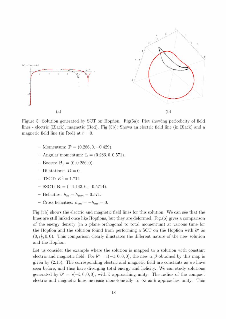
• Conformal transformations:
We used the conformal transformation (3.12) to generate new solutions from the plane
wave. The action of such transformation on the Hopfion solution can generate new so-
lutions with finite energy and helicity for some finite range of values of the parameter
of the transformation. Let us consider bµ as (0, i12, 0, 0). We can compute the charges
numerically for E = 1
17
2 4 6 8 10 12Τ
-15
-10
- 5
lnH È xiH ΤL - xiH 0L ÈL
(a)
-1
0
1
2
x
-1
0
1
2
y- 2
-1
0
1
z
(b)
Figure 5: Solution generated by SCT on Hopfion. Fig(5a): Plot showing periodicity of field
lines - electric (Black), magnetic (Red). Fig.(5b): Shows an electric field line (in Black) and a
magnetic field line (in Red) at t = 0.
– Momentum: P = (0.286, 0,−0.429).
– Angular momentum: L = (0.286, 0, 0.571).
– Boosts: Bv = (0, 0.286, 0).
– Dilatations: D = 0.
– TSCT: K0 = 1.714
– SSCT: K = (−1.143, 0,−0.5714).
– Helicities: hee = hmm = 0.571.
– Cross helicities: hem = −hme = 0.
Fig.(5b) shows the electric and magnetic field lines for this solution. We can see that the
lines are still linked once like Hopfions, but they are deformed. Fig.(6) gives a comparison
of the energy density (in a plane orthogonal to total momentum) at various time for
the Hopfion and the solution found from performing a SCT on the Hopfion with bµ as
(0, i12, 0, 0). This comparison clearly illustrates the different nature of the new solution
and the Hopfion.
Let us consider the example where the solution is mapped to a solution with constant
electric and magnetic field. For bµ = i(−1, 0, 0, 0), the new α, β obtained by this map is
given by (2.15). The corresponding electric and magnetic field are constants as we have
seen before, and thus have diverging total energy and helicity. We can study solutions
generated by bµ = i(−b, 0, 0, 0), with b approaching unity. The radius of the compact
electric and magnetic lines increase monotonically to ∞ as b approaches unity. This
18
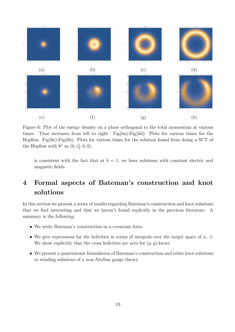
(a) (b) (c) (d)
(e) (f) (g) (h)
Figure 6: Plot of the energy density on a plane orthogonal to the total momentum at various
times. Time increases from left to right. Fig(6a)-Fig(6d): Plots for various times for the
Hopfion. Fig(6e)-Fig(6h): Plots for various times for the solution found from doing a SCT of
the Hopfion with bµ as (0, i12, 0, 0).
is consistent with the fact that at b = 1, we have solutions with constant electric and
magnetic fields.
4 Formal aspects of Bateman’s construction and knot
solutions
In this section we present a series of results regarding Bateman’s construction and knot solutions
that we find interesting and that we haven’t found explicitly in the previous literature. A
summary is the following:
• We write Bateman’s construction in a covariant form.
• We give expressions for the helicities in terms of integrals over the target space of α, β.
We show explicitly that the cross helicities are zero for (p, q)-knots.
• We present a quaternionic formulation of Bateman’s construction and relate knot solutions
to winding solutions of a non-Abelian gauge theory.
19
4.1 Covariant formulation
Our goal is to write the equations (2.3) and (2.5) in a covariant way5. We will be using mostly
plus signature for the space-time metric. The Levi-Civita symbol is defined as,
εijk = εijk. (4.1)
Eq. (2.3) can be written as,
Ei + iBi = εijk∂iα∂jβ. (4.2)
Rewriting the equation above in terms of the anti-symmetric field strength (Fµν),
F 0i + i1
2εijkFjk = εijk∂iα∂jβ. (4.3)
where we have used Ei = F 0i and Bi = 12εijkFjk . This can be written in covariant form as,
F µν − i12εµναβFαβ = −εµνρσ∂ρα∂σβ. (4.4)
where we define the epsilon tensor as,
ε0ijk = εijk; ε0ijk = −εijk. (4.5)
Now the (i, j)-components of the Eq. (4.4) are
F ij − iεijk0Fk0 = −εijk0(∂kα∂0β − ∂0α∂kβ). (4.6)
This is the same as,
εijkBk − iεijkEk = εijk(∂tα∂kβ − ∂kα∂tβ). (4.7)
which is equivalent to,
Bk − iEk = (∂tα∂kβ − ∂kα∂tβ). (4.8)
Multiplying both sides by i,
Ek + iBk = i(∂tα∂kβ − ∂kα∂tβ). (4.9)
which is the same as Eq. (2.5). Therefore (4.4) contains all the information about the equations
of motion. If we use the identity,
εµνρ1σ1εµνρ2σ2 = −2
(δρ2ρ1δ
σ2σ1− δσ2ρ1 δ
ρ2σ1
), (4.10)
we can show that the combination of field strengths appearing in Bateman’s construction is
imaginary anti-self dual
− i12εσρµν
[F µν − i1
2εµναβFαβ
]= F σρ − i1
2εσραβFαβ. (4.11)
5It was pointed out by an unknown referee that covariant formulation of Bateman construction was also
considered in [34].
20
We can also obtain covariant formulas for the potentials in terms of α and β. From (4.4),
F µν = −εµνρσRe (∂ρα∂σβ) , (4.12)
εµναβFαβ = 2εµνρσIm (∂ρα∂σβ) . (4.13)
We can rewrite the second equation (4.13) as,
Fµν = Im (∂µα∂νβ − ∂να∂µβ)
= ∂µAν − ∂νAµ, (4.14)
where,
Aµ = Im (Hµ) ; Hµ =1
2(α∂µβ − β∂µα) . (4.15)
The expression of the gauge potential Aµ or the complex potential Hµ is unique up to gauge
transformations. We can also define a complex field strength corresponding to Hµ as Hµν =
∂µHν − ∂νHµ, so that Fµν = Im (Hµν).
Similarly let us define Cµ and Gµν as,
Gµν =1
2εµνρσF
ρσ = ∂µCν − ∂νCµ. (4.16)
Then, up to a gauge choice,
Cµ = Re (Hµ) . (4.17)
Spatial components of Aµ, Cµ and related to electric and magnetic fields as,
Ei = εijk∂jCk ; Bi = εijk∂jAk. (4.18)
Then the first equation (4.12) can be rewritten in terms of the complex field strength as,
Im (Hµν) = −1
2εµνρσRe (Hρσ) (4.19)
The equation above along with the definition of Hµν in terms of the potential is equivalent to
Maxwell’s equations of motion. We can also define a helicity or Abelian Chern Simons current
as,
κµ = εµνρσAνFρσ. (4.20)
We can show that this current is conserved for the null solutions as,
∂µκµ =
1
2εµνρσFµνFρσ ∝ E ·B = 0. (4.21)
also,
κ0 = −εijkAiFjk = −2AiBi ; hmm = −1
2
∫d3xκ0 (4.22)
21
4.2 Helicities
In most cases we have to compute the conserved charges of a given solution by evaluating the
charge densities on the solution and doing a complicated integral over space. This makes the
comparison between different kind of solutions quite cumbersome. However, for the (p, q)-knots
it turns out that the situation is dramatically improved for the helicities. Indeed, one can find
closed expressions in terms of integrals over the target space, which are valid independently of
the particular form of the solution in space and time. It is even possible to prove that the cross
helicities vanish, as we will do in the following.
Let us define the complex two-form field H, related to the electromagnetic field strength F
(not to be confused with RS vector F) as
H = iF + ?F = df ∧ dg, (4.23)
where ? represents Hodge dual, which in terms of the components,
(?F )µν =1
2εµνρσF
ρσ. (4.24)
The relation to the complex vector F = E + iB is
Hi0 = i(F)i, Hij = iεijk(F)k. (4.25)
It will be convenient to solve the field strength and the dual in terms of the complex form H,
F =H − H
2i(4.26)
?F =H + H
2(4.27)
where H is the complex conjugate of H. Let F = dA, ?F = dC and H = dh. Then, the
potentials can be written in the following form
A =h− h
2i, (4.28)
C =h+ h
2, (4.29)
h =1
2(fdg − gdf). (4.30)
The cross helicity density hem is given by space integral of the following expression,
χem = C ∧ F =1
4i
(h ∧H − h ∧ H
). (4.31)
For (p, q)-knot solutions we simply need to evaluate χem for f = αp, g = βq,
h =1
2(αpd(βq)− βqd(αp)) = αp−1βq−1 1
2(qαdβ − pβdα), (4.32)
H = d(αp) ∧ d(βq) = pqαp−1βq−1dα ∧ dβ, (4.33)
|α|2 + |β|2 = 1. (4.34)
22
Substituting above in Eq. (4.31),
χem =pq
8i|α|2(p−1)|β|2(q−1)
(q d(αα) ∧ dβ ∧ dβ + p d(ββ) ∧ dα ∧ dα
)= 0. (4.35)
Where we have used Eq. (4.34) to show that it vanishes. Since hem = −hme, both the cross
helicities are zero for this class of solutions.
The helicity (hmm) is given by space integral of the following form,
χmm = A ∧ F =1
4
(h ∧ H + h ∧H
). (4.36)
Let us try to evaluate χ again for solutions of type (f = αp, g = βq) where α, β satisfies
Eq. (4.34). H, h are given by Eq. (4.33) and (4.32). We can parametrize α, β as,
α = cos(φ)eiθ1 , (4.37)
β = sin(φ)eiθ2 , (4.38)
dα = − sin(φ)eiθ1dφ+ i cos(φ)eiθ1dθ1, (4.39)
dβ = cos(φ)eiθ2dφ+ i sin(φ)eiθ2dθ2. (4.40)
From these formulas we can show,
dβ ∧ dα ∧ dα = −2 sin2(φ) cos(φ)eiθ2dφ ∧ dθ1 ∧ dθ2, (4.41)
dα ∧ dβ ∧ dβ = −2 sin(φ) cos2(φ)eiθ1dφ ∧ dθ1 ∧ dθ2. (4.42)
(4.43)
Also,
χmm =pq
8|α|2(p−1)|β|2(q−1)
(qαdα ∧ dβ ∧ dβ + pβdβ ∧ dα ∧ dα + cc
)(4.44)
= −pq2
cos2p−1 φ sin2q−1 φ(q cos2 φ+ p sin2 φ
)dφ ∧ dθ1 ∧ dθ2. (4.45)
Note that α and β for the Hopfion solution at time t = 0 are simply the inverse of the stereo-
graphic projection of the three-sphere |α|2 + |β|2 = 1 onto the space. Since this is a one-to-one
mapping, we can trade the integral over space for an integral over the S3 parametrized by α
and β. Then,
hmm = −∫S3
χmm
=4π2pq
2
∫ π/2
0
dφ(q cos2p+1 φ sin2q−1 φ+ p cos2p−1 φ sin2q+1 φ
). (4.46)
Now, using the identity ∫ π/2
0
dθ sin(θ)m cos(θ)n =Γ(m+1
2)Γ(n+1
2)
2Γ(n+m+22
), (4.47)
we find the following value of the helicity
hmm = 2π2pqΓ(p+ 1)Γ(q + 1)
Γ(p+ q + 1)= 2π2pq
p!q!
(p+ q)!. (4.48)
23
for p = q = 1,∫S3 χ = π2. Note the result is symmetric under interchange of (p, q). For more
general holomorphic functions of α, β satisfying Eq. (4.34), we find the following expressions
for the helicity density :
h =1
2(f(α, β)d(g(α, β))− g(α, βd(f(α, β)) , (4.49)
H = d(f(α, β)) ∧ d(g(α, β), (4.50)
χmm =1
2
[Re
((∂αf∂βg − (∂αg∂βf)(f∂αg − g∂αf)
β
)sin3(φ) cos(φ)
− Re
((∂αf∂βg − (∂αg∂βf)(f∂βg − g∂βf)
α
)sin(φ) cos3(φ)
]dφ ∧ dθ1 ∧ dθ2. (4.51)
4.3 Quaternionic Formulation and Map to Non Abelian theories
There is an interesting map between Bateman’s construction and quaternions that can be used
to embed the Hopfion solution in a non-Abelian Yang-Mills theory. The non-Abelian solution
is pure gauge with winding number different than zero. Similar embeddings of knot solutions
were studied in the past [29–31], the main differences in this case are that the knot is not static
and that it is a solution of Maxwell’s theory.
Using α and β we can define a quaternion q,
q =1
m(α + βj), (4.52)
m =√|α|2 + |β|2, (4.53)
α = α0 + α1i ; β = β0 + β1i, (4.54)
where α0, α1, β0, β1 are real functions depending on space-time. The conjugate quaternion is
q∗ =1
m(α∗ − βj). (4.55)
We will define the following quaternionic-valued potential:
Qµ = q(∂µq∗). (4.56)
We can easily show that,
Qµ = −Q∗µ (4.57)
We will write the components of the quaternionic potential in the following form:
Qµ =1
m2Im (α∂µα
∗ + β∂µβ∗)i− 2
m2Hµj. (4.58)
where the complex potential Hµ is defined in (4.15).
Associated to the quaternionic potential we can define a quaternionic field strength,
Qµν = ∂µQν − ∂νQµ = (∂µq∂νq∗ − ∂νq∂µq∗) . (4.59)
24
Then,
Qµν =2
m2Im (∂µα∂να
∗ + ∂µβ∂νβ∗) i− 2
m2Hµνj + Jµν (4.60)
Jµν = m2∂µ(1
m2)Qν −m2∂ν(
1
m2)Qµ (4.61)
Note that Jµν = 0 for cases where m is constant. The equation of motion given by (4.19) can
be rewritten as,
(Qµν − Jµν)k = −1
2εµνρσ(Qρσ − Jρσ)j, (4.62)
Since,
qq∗ = 1. (4.63)
Then we can show,
Qµν = ∂µQν − ∂νQµ = − [Qµ,Qν ] . (4.64)
Note that we can interpret (4.56) as a non-Abelian SU(2) gauge potential by using Pauli
matrices as a representation of the quaternion components 1, i, j, k
1 ≡ 12×2, i ≡ −iσ1, j ≡ −iσ2, k ≡ −iσ3. (4.65)
Using (4.64) it is clear that the non-Abelian field strength is zero, and therefore this is a pure
gauge solution. We will show now that the winding number is non-zero, and in fact it is directly
related to the helicities of the Abelian solution.
4.3.1 Winding number of non-Abelian solutions
The winding number of non-Abelian solutions is measured by the integral over space of the
Chern-Simons three-form
w = − 1
8π2
∫S3
tr (K) , (4.66)
where the Chern-Simons three form is
K = Q ∧ dQ +2
3Q ∧Q ∧Q. (4.67)
For smooth pure gauge non-Abelian configurations in a compact space w is an integer. We
can define a current one-form using the Hodge dual JCS = ?K. We can show that the current
is conserved when the non-Abelian pure gauge configuration is obtained from a null Abelian
solution obeying Eq. (4.64) (dQ = −Q ∧Q)
?d?JCS = ?dK = ?(dQ + Q ∧Q) ∧ (dQ + Q ∧Q)− ?(Q ∧Q ∧Q ∧Q)
= −?(dQ ∧ dQ) ∝ E ·B = 0. (4.68)
The non-Abelian Chern-Simons current for a solution obeying Eq. (4.64) is
JCS =1
3?(Q ∧ dQ). (4.69)
25
In components, this is
JCSµ =
1
6εµνρσQνQρσ =
1
3εµνρσQνQρQσ. (4.70)
Using Q∗µ = −Qµ we can show,
JCSµ = (JCS
µ)∗. (4.71)
Let us evaluate JCSµ in terms of components,
JCSµ = −1
6εµνρσ
∑a∈{i,j,k}
(Qν)a(Qρσ)a + · · · (4.72)
The · · · denotes terms that are proportional to i, j, k, which we can set to zero even without
calculation as JCSµ is real. Now using (4.61),
JCSµ = −1
6εµνρσ
∑a∈{i,j,k}
(Qν)a(Qρσ − Jρσ)a (4.73)
We can show (there is no summation over the index a),
εµνρσ(Qν)a(Qρσ − Jρσ)a =4
m2εµνρσAνFρσ12×2 =
4
m2κµ12×2 ∀a ∈ (i, j, k), (4.74)
where κµ (4.20) is the Abelian Chern Simons current. So the relation between Abelian and
non-Abelian (quaternionic) Chern Simons is given by,
JCSµ =
2
m4κµ12×2. (4.75)
Both of the currents, JCSµ and κµ were shown to be conserved in (4.68) and (4.21). This gives
a non-trivial constraint on the derivative of m : κµ∂µm = 0.
For α = αp, β = βq with |α|2 + |β|2 = 1,∫d3xκ0 = 2
∫χmm is calculated for these solutions
in Eq. (4.45). Then the corresponding winding number of the non-Abelian solution is given by
w = − 1
8π2
∫S3
trJCS0 = −2
1
8π2
∫S3
4
m4χmm
= 21
8π2
∫ π/2
0
dφ4
(cos(φ)2p + sin(φ)2q)2
4π2pq
2
(q cos2p+1 φ sin2q−1 φ+ p cos2p−1 φ sin2q+1 φ
)= pq. (4.76)
In contrast with the values of the Abelian helicities, which were not integers, the corre-
sponding non-Abelian winding number is quantized in integer values. Note that the Hopfion
solution has winding number w = 1 as expected. We can also use the Abelian Hopfion solution
to construct higher winding non-Abelian solutions. Consider the non- Abelian (quaternionic)
potential,
Qµ = q(∂µq∗) (4.77)
where,
q = α + βj = qn = (α + βj)n (4.78)
26
Note,
qq∗ = (qq∗)n = 1 (4.79)
and α, β are given by the Abelian solution Eq. (2.19) and Eq. (2.20). The non-Abelian gauge
potential Qµ naturally gives a flat gauge connection due to its structure. We expect these to
be solutions with winding number n-times that of the solution with potential given by q, we
have checked for n = 2 that it is indeed the case. These higher winding non-Abelian solutions
α and β are not solutions of Maxwell’s equations.
5 Summary
In this note we have further developed the study of topologically non-trivial solutions of elec-
trodynamics. We have discovered a novel method of generating such solutions by applying
conformal transformations with complex parameters on known solutions expressed in terms of
Bateman’s variables. This enabled us in fact to get a wide class of solutions from the basic
configuration of constant electric and magnetic fields. We have introduced a covariant formu-
lation of the Bateman’s construction and discussed the conserved charges associated with the
conformal group as well as a set of four types of conserved helicities. One way to implement
the covariant formulation is to use a quaternionic formulation. This led to a simple map be-
tween the electromagnetic knotted solutions into flat connections of SU(2) gauge theory. We
computed the corresponding CS charge and show that it takes an integer value.
There is an ample variety of open questions related to the study of the knotted solutions of
electrodynamics. Here we mention few of them.
• Obviously the most interesting issue is how to realize the Hopfion or any of its cousins in
the Laboratory. The question is whether we can supply our experimental colleagues with
additional information that will enable them to produce these non-trivial electromagnetic
configurations. A proposal for constructing Hopf solutions in laboratory was given in [8].
• The solutions discussed in this note, from the constant E and B and all the way to
the generalization of the Hopfions were expressed in Cartesian coordinates. Obviously
there are electromagnetic configurations that are naturally described in cylindrical and
spherical coordinates. One can search for their expressions in terms of the Bateman’s
variables which will now be complex functions of spherical or cylindrical or more general
coordinates. Performing the conformal transformation with complex coordinates can also
be done using various different coordinate systems.
• An interesting question is obviously deciphering the trajectories of charged particles in the
topologically non-trivial EM fields. Do these trajectories admit some topology? A class
of charged particle trajectories in Hopfion background was studied numerically in [10].
A more general question is looking for similar topological solutions to the equations of
motion of electrodynamics coupled to currents and charge densities.
• A more theoretical issue is the classification of all solutions that follow from Bateman’s
construction. The class of solutions based on taking any holomorphic function of the
27
basic Hopfion α and β, as well as all other solutions that one gets by applying all possible
conformal transformations with complex parameters.
• A similar issue relates to the classification of the corresponding SU(2) flat gauge con-
nections. Are there SU(2) flat gauge connections that cannot be mapped into the EM
topologically non-trivial configurations? and if yes what characterize those that can be
mapped.
• We have mentioned that the solutions found in this note are in fact valid in any conformal
flat background of which AdS4 (Anti-de Sitter 4-d space-time) is a special case. One may
wonder in the context of holography [35], [36], [37] with electromagnetic fields in the bulk
what are the corresponding dual (topological?) configurations on the boundary conformal
field theory.
6 Acknowledgments
J.S would like to thank Ori Ganor for useful discussions. We would like to acknowledge the
useful comments and suggestion from unknown referees. The work of N.S was supported by
”The PBC program for fellowships for outstanding post-doctoral researcher from China and
India of the Israel council of higher education”. This work was partially supported by the
Israel Science Foundation (g rant 1989/14),the US-Israel bi-national fund (BSF) grant number
2012383 and the GermanyIsrael bi-national fund GIF grant number I-244-303.7-2013. This
work is partially supported by the Spanish grant MINECO-13-FPA2012-35043-C02-02. C.H. is
supported by the Ramon y Cajal fellowship RYC-2012-10370.
A Noether Charges
Let us consider a gauge potential Aµ and the corresponding field strength Fµν = ∂µAν−∂νAµto be solutions of 4-d vacuum Maxwell equations ∂µF
µν = 0. The electric and magnetic field
are given by,
Ei = F 0i = Fi0 (A.1)
Bi =1
2εijkFjk or Fjk = εijkB
i (A.2)
where we have assumed mostly positive signature for the space-time metric. Then,
− 1
4FµνF
µν =1
2(E · E−B ·B) (A.3)
The stress-energy tensor is
Tµν = −FµρF ρν +
1
4ηµνFαβF
αβ (A.4)
28
Explicit expressions of the components of stress energy tensor are
T00 =1
2(E · E + B ·B) (A.5)
T0i = −(E×B)i (A.6)
Tij = δij1
2(E · E + B ·B)− EiEj −BiBj (A.7)
The stress energy tensor satisfies,
∂µTµν = 0 ; T µµ = 0 (A.8)
Then the list of conserved charge densities from conservation of stress tensor are given by,
Energy: E = T 00 =1
2(E · E + B ·B) (A.9)
Momentum : pi = T 0i = (E×B)i (A.10)
Now let us consider the conserved current corresponding to the Lorentz symmetry,
Jµ(αβ)Λ = T µαxβ − T µβxα (A.11)
∂µJµ(αβ)Λ = T βα − Tαβ = 0 (A.12)
using the symmetry properties of the stress tensor. The corresponding charges are given by,
J0(αβ)Λ , which is antisymmetric in (α, β). Then the spatial and temporal charges given by J
0(αβ)Λ
is,
Momentum : li =∑jk
εijkJ0(jk)Λ = (p× x)i (A.13)
Boost : bi = J0(0i)Λ = Exi − pit (A.14)
Now consider the current corresponding to dilatation symmetry,
JµD = T µν xν (A.15)
∂µJµD = T µµ = 0 (A.16)
The corresponding conserved charge density is given by,
Dilatation : d = J0D = −Et+
∑i
pixi (A.17)
Now let us consider the current corresponding to the special conformal transformation,
Jµ(ν)k = xαxαT
µν − 2T µρ xρxν (A.18)
∂µJµ(ν)k = −2T µµ x
ν = 0 (A.19)
Then the corresponding temporal and spatial charges are given by,
TSCT: k0 = Jµ(0)k = (xixi + t2)E − 2tpix
i (A.20)
SSCT: ki = −Jµ(i)k = 2xipjx
j − 2Etxi − (xixi − t2)pi (A.21)
29
B θ, φ Formulation
B.1 Hopf index in 3-dimensions
Consider a complex scalar field φ(x1, x2, x3) defined on R3. Let the field be well defined as
r → ∞, where r =√x2
1 + x22 + x2
3, i.e. the map does not depend on the direction. Then the
map can be identified as φ : S3 → S2, as S3 ≡ R3 ∪ {∞} and S2 ≡ C1 ∪ {∞}. These class
of maps are generally classified in various homotopy classes specified by a topological invariant
called Hopf index.
Consider the area two form [5],
F =1
2πi
dφ∗ ∧ dφ(1 + φφ∗)2
(B.1)
Since F is closed in S3, it must also be exact, i.e. there is a one form A such that F = dA.
Then the Hopf index is given by [1],
n =
∫S3
A ∧ F (B.2)
The pull back of the form F in R3 is given by,
F =1
2Fijdx
i ∧ dxj =1
4πi
∂iφ∗∂jφ− ∂jφ∗∂iφ(1 + φφ∗)2
dxi ∧ dxj (B.3)
We can also express F in terms of a vector field defined as,
Bi = Bi =1
2εijkFjk (B.4)
B = Bidxi = W (φ) is called the Whitehead vector of the map φ. By definition, B · ∇φ = 0,
i.e. the vector B is always tangential to the surfaces φ = constant.
Let us parametrize the map φ as,
φ = Se2πiψ ; ρ = − 1
1 + S2(B.5)
where S, ψ, ρ are real maps from R3 → R. then,
F = dρ ∧ dψ ; A = ρdψ + dξ (B.6)
ξ is some arbitrary function from R3 → R. Then,
n =
∫S3
d(ξdρ ∧ dψ) (B.7)
is zero by Gauss’ theorem unless ψ or ρ is multiple valued. We will assume ψ to be multiple
valued, and ∇ψ to be a single valued function.
Hopf Map A simplest example of a map φ : S3 → S2 with non zero Hopf index is
φH(x, y, z) =2(x+ iy)
2z + i(r2 − 1); r2 = x2 + y2 + z2 (B.8)
The Hopf index is unity for this map.
30
B.2 (n,m)-link solutions in 3 + 1-dimension
Now consider two such maps φ, θ : S3×R→ S2. Then let us consider the electric and magnetic
field to be Whitehead vectors of the two maps, B = W (φ) and E = W (θ). The maps now
depend on a extra time parameter, and to make the equations consistent with the 3 + 1-d
Maxwell equations,
Mµν =1
2εµνρσF
ρσ (B.9)
Fµν = fµν(φ) =1
2πi
∂µφ∗∂νφ− ∂νφ∗∂µφ(1 + φφ∗)2
(B.10)
Mµν = fµν(θ) =1
2πi
∂µθ∗∂νθ − ∂νθ∗∂µθ(1 + θθ∗)2
(B.11)
where 6,
Ei = Fi0 =1
2εijkM
jk ; Bi = M0i =1
2εijkF
jk (B.12)
Note our definitions are the same as that of [5] up to some signs. For solutions parametrized
as (B.9)-(B.11), we can show,
E ·B =1
2εijkM0iM
jk = −1
2εµνρσMµνMρσ = 0 (B.13)
as a consequence the helicities defined (B = ∇×A and E = ∇×C) as,
he =
∫S3
A ·B (B.14)
hm =
∫S3
C · E (B.15)
are time independent. Also these are proportional to the Hopf Index (B.2) of the two maps θ
and φ. Since Hopf Indices are integers, the helicities will be given by integer multiple of some
constant number.
Hopfion I The simplest solution with he = hm is given by [4], [6], [8],
φ =(Az + t(A− 1)) + i(tx− Ay)
(Ax+ ty) + i(A(A− 1)− tz)(B.16)
θ =(Ax+ ty) + i(Az + t(A− 1))
(tx− Ay) + i(A(A− 1)− tz)(B.17)
A =1
2(x2 + y2 + z2 − t2 + 1) (B.18)
which at t = 0 reduces to Hopf map (B.8),
φ(t = 0, x, y, z) =2(z − iy)
2x+ i(r2 − 1)= φH(z,−y, x) (B.19)
θ(t = 0, x, y, z) =2(x+ iz)
−2y + i(r2 − 1)= φH(x, z,−y) (B.20)
6we define ε0ijk = −ε0ijk = εijk = εijk
31
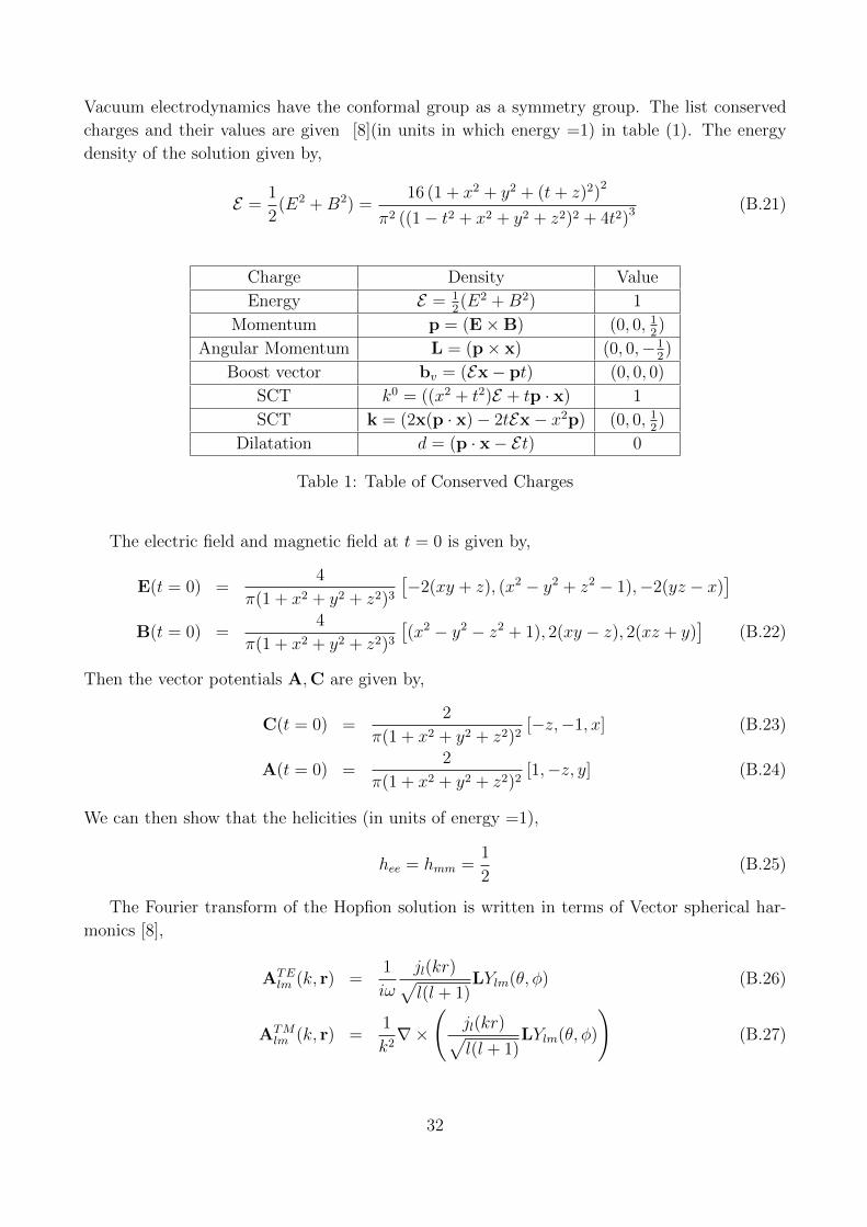
Vacuum electrodynamics have the conformal group as a symmetry group. The list conserved
charges and their values are given [8](in units in which energy =1) in table (1). The energy
density of the solution given by,
E =1
2(E2 +B2) =
16 (1 + x2 + y2 + (t+ z)2)2
π2 ((1− t2 + x2 + y2 + z2)2 + 4t2)3 (B.21)
Charge Density Value
Energy E = 12(E2 +B2) 1
Momentum p = (E×B) (0, 0, 12)
Angular Momentum L = (p× x) (0, 0,−12)
Boost vector bv = (Ex− pt) (0, 0, 0)
SCT k0 = ((x2 + t2)E + tp · x) 1
SCT k = (2x(p · x)− 2tEx− x2p) (0, 0, 12)
Dilatation d = (p · x− Et) 0
Table 1: Table of Conserved Charges
The electric field and magnetic field at t = 0 is given by,
E(t = 0) =4
π(1 + x2 + y2 + z2)3
[−2(xy + z), (x2 − y2 + z2 − 1),−2(yz − x)
]B(t = 0) =
4
π(1 + x2 + y2 + z2)3
[(x2 − y2 − z2 + 1), 2(xy − z), 2(xz + y)
](B.22)
Then the vector potentials A,C are given by,
C(t = 0) =2
π(1 + x2 + y2 + z2)2[−z,−1, x] (B.23)
A(t = 0) =2
π(1 + x2 + y2 + z2)2[1,−z, y] (B.24)
We can then show that the helicities (in units of energy =1),
hee = hmm =1
2(B.25)
The Fourier transform of the Hopfion solution is written in terms of Vector spherical har-
monics [8],
ATElm (k, r) =
1
iω
jl(kr)√l(l + 1)
LYlm(θ, φ) (B.26)
ATMlm (k, r) =
1
k2∇×
(jl(kr)√l(l + 1)
LYlm(θ, φ)
)(B.27)
32
where L = −ir × ∇, Ylm(θ, φ) are spherical harmonics, jl(kr) are spherical Bessel functions.
Also l ≥ 1 and −l < m < l. Then the vector potential (B = ∇× A) for the Hopfion is given
by [4] [8],
A(r, t) =
∫ ∞0
dk (A(k, r) + A(k, r)∗) (B.28)
A(k, r) =
√4
3πk3e−k
[ATE
1,1 (k, r)− iATM1,1 (k, r)
]e−iωt (B.29)
The superposition[ATE − iATM
]is an eigenstate of curl operator and are known as Chandrasekhar-
Kendall states.
∇×[ATEl,m(k, r)± iATM
l,m (k, r)]
= ∓k[ATEl,m(k, r)± iATM
l,m (k, r)]
(B.30)
The corresponding electric and magnetic fields are then given by,
B(k, r) = ∇× (A(k, r) + A(k, r)∗) = k (A(k, r) + A(k, r)∗) (B.31)
E(k, r) = −∂t (A(k, r) + A(k, r)∗) = iω (A(k, r)−A(k, r)∗) (B.32)
Generalization to (p, q)-knots in (θ, φ) formulation There were various attempts to con-
struct general knotted solution with preserved topological structure in [9], [12]. But although
helicity was conserved, the topological structure varies with time in the class of solution de-
scribed in [9], [12]. In a recent paper [14], authors were able to construct solutions using
Bateman’s construction [2] knotted solutions which preserves its structure over time. Let us
describe the prescription given in [9]. We can easily generalize to (p, q)-knots by modifying
Eq. (B.29) as given in [9],
A(k, r) =
√4
3πk3e−k
[ATE
1,1 (k, r)− ipqATM
1,1 (k, r)
]e−iωt (B.33)
For general (p, q) co-prime integers, this corresponds to all possible Knots. A important point
about these solution as emphasized in [9], is that E ·B 6= 0 but∫d3xE ·B = 0. So these cases
the helicity is conserved but if we look at the topological structure of individual field lines, it
changes with time. So the knot structure implied by co-prime integers (p, q) is only valid at
t = 0.
C Explicit expression of electric and magnetic field for
Hopfion
The Riemann-Silberstein vector for the Hopfion solution given by (2.19),(2.20) is,
F =4
(A+ 2it)3
(t− x− z + i(y − 1))(t+ x− z − i(y + 1)
−i(t− y − z − i(x+ 1))(t+ y − z + i(x− 1))
2(x− iy)(t− z − i)
(C.1)
33
where A = (x2 + y2 + z2− t2 + 1). The electric and magnetic field can be read of directly from
F as the real and imaginary part respectively. Generally the expressions of the electric and
magnetic field looks complicated but can be written in a more compact form as polynomial in
A. We illustrate that for one of the components for the electric field,
Ex = −4[A4 − 2A3(y2 + z2 − tz)− 12A2t(xy + z) + 24At2(y2 + z2 − tz)
+16t3(−t+ xy + z)]/(A2 + 4t2)3. (C.2)
For t = 0 this reduces to
Ex(t = 0) = − 4
(1 + r2)3(1 + x2 − y2 − z2) (C.3)
which is identical to Ey of (B.22) upon interchanging x↔ y. At the origin ~r = 0 we find
Ex = −4(1− 3t2)
(1 + t2)3(C.4)
34
References
[1] J. H. Whitehead, “An Expression of Hopf’s Invariant as an Integral”, Proc Natl Acad Sci
U S A. 1947 May;33(5):117-23.
[2] H. Bateman, “The Mathematical Analysis of Electrical and Optical Wave-motion on the
Basis of Maxwell’s Equations,” University Press, 1915.
[3] A. F. Ranada, “A Topological Theory of the Electromagnetic Field,” Lett. Math. Phys.
18, 97 (1989).
[4] A. F. Ranada, “Knotted solutions of the Maxwell equations in vacuum,” J. Phys. A:
Math. Gen. 23, L815 (1990).
[5] A. F. Ranada, “Topological electromagnetism,” J. Phys. A 25, 1621 (1992).
[6] A. F. Ranada, Jose L. Trueba, “Electromagnetic knots,” Phys. Lett. A 202 (1995)
337342.
[7] A. F. Ranada, Jose L. Trueba, “Two properties of electromagnetic knots,” Phys. Lett.
A 232 (1997) 25-33.
[8] W.T.M. Irvine, D. Bouwmeester, “Linked and knotted beams of light,” (2008) Nature
Physics, 4 (9), pp. 716-720.
[9] W.T.M. Irvine, “Linked and knotted beams of light, conservation of helicity and the
flow of null electromagnetic fields ,” J. Phys. A: Math. Theor. 43 (2010) 385203,
arXiv:1110.5408 [physics.optics].
[10] M. Arrayas, J.L. Trueba, “Motion of charged particles in a knotted electromagnetic field,”
J. Phys. A: Math. Theor. 43 235401, arXiv:1001.4985 [math-ph].
[11] M. Arrayas and J. L. Trueba, “Exchange of helicity in a knotted electromagnetic field,”
Annalen Phys. 524, 71 (2012) [arXiv:1105.6285 [hep-th]].
[12] M. Arrayas and J. L. Trueba, “Electromagnetic Torus Knots,” arXiv:1106.1122 [hep-th].
[13] Ioannis M. Besieris and Amr M. Shaarawi , “HopfRanada linked and knotted light
beam solution viewed as a null electromagnetic field”, Optics Letters, Vol. 34, Issue 24,
pp. 3887-3889 (2009).
[14] Hridesh Kedia, Iwo Bialynicki-Birula, Daniel Peralta-Salas, William T. M. Irvine, “Tying
Knots in Light Fields”, Phys. Rev. Lett. 111, 150404 (2013), arXiv:1302.0342 [math-ph].
[15] J. W. Dalhuisen and D. Bouwmeester, “Twistors and electromagnetic knots,” J. Phys. A
45, 135201 (2012).
[16] J. Swearngin, A. Thompson, A. Wickes, J. W. Dalhuisen and D. Bouwmeester, “Gravita-
tional Hopfions,” arXiv:1302.1431 [gr-qc].
35
[17] A. Thompson, J. Swearngin and D. Bouwmeester, “Linked and Knotted Gravitational
Radiation,” J. Phys. A 47, 355205 (2014) [arXiv:1402.3806 [gr-qc]].
[18] A. Thompson, A. Wickes, J. Swearngin and D. Bouwmeester, “Classification of Electro-
magnetic and Gravitational Hopfions by Algebraic Type,” arXiv:1411.2073 [gr-qc].
[19] M. Arrayas and J. L. Trueba, “A class of non-null toroidal electromagnetic fields and
its relation to the model of electromagnetic knots”, J. Phys. A: Math. Theor. 48 025203
(2015).
[20] http://www.hopfion.com
[21] Iwo Bialynicki-Birula, ”The photon wave function, ” Coherence and Quantum Optics VII.
Springer US, 1996. 313-322.
[22] A. Trautman, ”Analytic solutions of Lorentz-invariant linear equations,” Proceedings of
the Royal Society of London. Series A, Mathematical and Physical Sciences (1962): 326-
328.
[23] Ezra T. Newman, ”Maxwell’s equations and complex Minkowski space,” J. Math. Phys.
14 102-103 (1973).
[24] Iwo Bialynicki-Birula, ”Electromagnetic vortex lines riding atop null solutions of the
Maxwell equations.” J. Opt. A: Pure Appl. Opt. 6 S181 (2004).
[25] Iwo Bialynicki-Birula and Zofia Bialynicka-Birula, ”The role of the RiemannSilberstein
vector in classical and quantum theories of electromagnetism,” J. Phys. A: Math. Theor.
46 053001 (2013), arXiv: 1211.2655 [physics.class-ph].
[26] V.I. Fouchtchitch and A.G. Nikitin, Symmetries of Maxwell’s equations, Springer, 1987.
[27] J.W. Dalhuisen, The Robinson congruence in electrodynamics and general relativity, PhD
thesis Leiden University (2014), https://openaccess.leidenuniv.nl/handle/1887/24880
[28] C. Codirla and H. Osborn, “Conformal invariance and electrodynamics: Applications and
general formalism,” Annals Phys. 260, 91 (1997) [hep-th/9701064].
[29] R. Jackiw and S. Y. Pi, “Creation and evolution of magnetic helicity,” Phys. Rev. D 61,
105015 (2000) [hep-th/9911072].
[30] P. van Baal and A. Wipf, “Classical gauge vacua as knots,” Phys. Lett. B 515, 181 (2001)
[hep-th/0105141].
[31] Y. M. Cho, “Knot topology of QCD vacuum,” Phys. Lett. B 644, 208 (2007) [hep-
th/0409246].
[32] N. S. Manton, “Scaling Identities for Solitons beyond Derrick’s Theorem,” J. Math. Phys.
50, 032901 (2009) [arXiv:0809.2891 [hep-th]].
36
[33] S. K. Domokos, C. Hoyos and J. Sonnenschein, “Deformation Constraints on Solitons and
D-branes,” JHEP 1310, 003 (2013) [arXiv:1306.0789 [hep-th]].
[34] S.J. Van Enk, “The covariant description of electric and magnetic field lines of null fields:
application to Hopf-Ranada solutions”, Journal of Physics A: Mathematical and Theoret-
ical vol.46, 17 (2013).
[35] J. M. Maldacena, “The Large N limit of superconformal field theories and supergrav-
ity,” Int. J. Theor. Phys. 38, 1113 (1999) [Adv. Theor. Math. Phys. 2, 231 (1998)] [hep-
th/9711200].
[36] S. S. Gubser, I. R. Klebanov and A. M. Polyakov, Phys. Lett. B 428, 105 (1998) [hep-
th/9802109].
[37] E. Witten, Adv. Theor. Math. Phys. 2, 253 (1998) [hep-th/9802150].
37