KNOTTED SOLUTIONS OF MAXWELL EQUATIONS

A THESIS SUBMITTED TOTHE GRADUATE SCHOOL OF NATURAL AND APPLIED SCIENCES

OFMIDDLE EAST TECHNICAL UNIVERSITY

BY

SALMAN EREN ALTUN

IN PARTIAL FULFILLMENT OF THE REQUIREMENTSFOR

THE DEGREE OF MASTER OF SCIENCEIN

PHYSICS

JULY 2019

Approval of the thesis:

KNOTTED SOLUTIONS OF MAXWELL EQUATIONS

submitted by SALMAN EREN ALTUN in partial fulfillment of the requirements forthe degree of Master of Science in Physics Department, Middle East TechnicalUniversity by,

Prof. Dr. Halil KalıpçılarDean, Graduate School of Natural and Applied Sciences

Prof. Dr. Altug ÖzpineciHead of Department, Physics

Prof. Dr. Bahtiyar Özgür SarıogluSupervisor, Physics, METU

Examining Committee Members:

Prof. Dr. Yıldıray OzanMathematics, METU

Prof. Dr. Bahtiyar Özgür SarıogluPhysics, METU

Assoc. Prof. Dr. Çetin SentürkAeronautical Engineering, UTAA

Date:

I hereby declare that all information in this document has been obtained andpresented in accordance with academic rules and ethical conduct. I also declarethat, as required by these rules and conduct, I have fully cited and referenced allmaterial and results that are not original to this work.

Name, Surname: Salman Eren Altun

Signature :

iv

ABSTRACT

KNOTTED SOLUTIONS OF MAXWELL EQUATIONS

Altun, Salman ErenM.S., Department of Physics

Supervisor: Prof. Dr. Bahtiyar Özgür Sarıoglu

July 2019, 54 pages

We review Rañada’s knotted solutions of Maxwell equations in this thesis. We ex-

plain the method behind these constructions and its relation to topology. The method

starts with the null field assumption. We obtain the initial conditions of the electro-

magnetic field using the Hopf map. Then we find the time-dependent fields using

Fourier transformation techniques. Finally, we analyze the properties of general torus

knotted solutions and show that these also include the non-null fields.

Keywords: electromagnetism, knotted solutions, Hopf map

v

ÖZ

MAXWELL DENKLEMLERININ DÜGÜMLÜ ÇÖZÜMLERI

Altun, Salman ErenYüksek Lisans, Fizik Bölümü

Tez Yöneticisi: Prof. Dr. Bahtiyar Özgür Sarıoglu

Temmuz 2019 , 54 sayfa

Bu tezde Rañada’nın buldugu, Maxwell denklemlerinin dügümlü çözümleri incelen-

mistir. Bu çözümlere ulasmak için kullanılan yöntem ve bunun topoloji ile iliskisi

açıklanmıstır. Çözümlere bos alan (Ing: null field) varsayımı ile baslanmıstır. Hopf

gönderimi (Ing: Hopf map) kullanılarak elektromanyetik alanın baslangıç kosulları

elde edilmistir. Daha sonra Fourier dönüsüm teknikleri kullanılarak zamana baglı

alanlar elde edilmistir. Son olarak genel simit dügümlü (Ing: torus knotted) çözüm-

lerin özellikleri irdelenmis, bunların bos olmayan (Ing: non-null) alanları da içerdigi

gösterilmistir.

Anahtar Kelimeler: elektromanyetizma, dügümlü çözümler, Hopf gönderimi

vi

to my family with love

vii

ACKNOWLEDGMENTS

I am deeply grateful to my supervisor, Prof. Dr. B.Özgür Sarıoglu for his dedication

and assistance during this work. The door to his office was always open whenever I

ran into a trouble or had a question about my research. I am very proud to have the

opportunity to meet and work with him.

I would like to say a heartfelt thank you to my wife Funda and beloved children

Defne and Demir for their understanding and patience. I would also like to thank

my mother, father and brother for their love and support. This would not have been

possible without them.

Finally, I would like to thank Üstünova Engineering and R&D, for their help in con-

ducting this study between the intense work pace.

viii

TABLE OF CONTENTS

ABSTRACT . . . . . . . . . . . . . . . . . . . . . . . . . . . . . . . . . . . . v

ÖZ . . . . . . . . . . . . . . . . . . . . . . . . . . . . . . . . . . . . . . . . . vi

ACKNOWLEDGMENTS . . . . . . . . . . . . . . . . . . . . . . . . . . . . . viii

TABLE OF CONTENTS . . . . . . . . . . . . . . . . . . . . . . . . . . . . . ix

LIST OF FIGURES . . . . . . . . . . . . . . . . . . . . . . . . . . . . . . . . xi

NOTATION . . . . . . . . . . . . . . . . . . . . . . . . . . . . . . . . . . . . xii

CHAPTERS

1 INTRODUCTION . . . . . . . . . . . . . . . . . . . . . . . . . . . . . . . 1

2 MAXWELL THEORY AND THE TOPOLOGICAL PROPERTIES OF AMONOPOLE FIELD . . . . . . . . . . . . . . . . . . . . . . . . . . . . . 5

2.1 Maxwell Equations . . . . . . . . . . . . . . . . . . . . . . . . . . . 5

2.2 Dirac Monopole . . . . . . . . . . . . . . . . . . . . . . . . . . . . 7

2.3 Gauge Transformation and Classical / Quantum Mechanical Effects . 10

2.4 Stereographic Projection and the n-Sphere . . . . . . . . . . . . . . 13

2.4.1 Stereographic Projection . . . . . . . . . . . . . . . . . . . . 13

2.4.2 The n-Sphere . . . . . . . . . . . . . . . . . . . . . . . . . . 15

2.5 Hopf Map and Trautman’s Proposal . . . . . . . . . . . . . . . . . . 16

3 TORUS KNOTS . . . . . . . . . . . . . . . . . . . . . . . . . . . . . . . . 19

3.1 Maxwell Equations as Geometric Identities . . . . . . . . . . . . . . 19

ix

3.2 Darboux Theorem and Clebsch Representation . . . . . . . . . . . . 21

3.3 Hopf Index and Magnetic Helicity . . . . . . . . . . . . . . . . . . . 27

3.4 Particle Interpretation of Electromagnetic Helicity . . . . . . . . . . 31

3.5 Rañada Construction using the Hopf Map . . . . . . . . . . . . . . . 33

3.5.1 Initial conditions for the knotted fields . . . . . . . . . . . . . 34

3.5.2 Time dependent knotted fields . . . . . . . . . . . . . . . . . 37

3.5.3 Interpretation of the knotted solutions and their properties . . . 44

4 CONCLUSIONS . . . . . . . . . . . . . . . . . . . . . . . . . . . . . . . 51

REFERENCES . . . . . . . . . . . . . . . . . . . . . . . . . . . . . . . . . . 53

x

LIST OF FIGURES

FIGURES

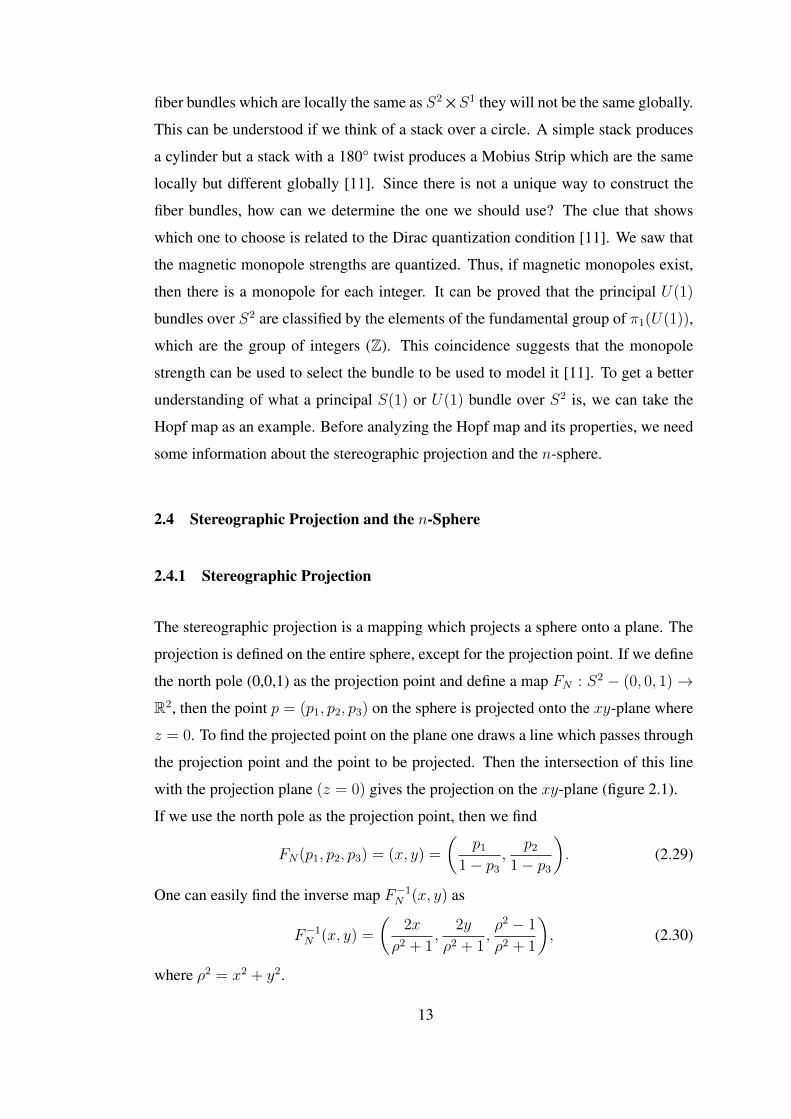
Figure 2.1 Stereographic projection from the north pole. . . . . . . . . . . . 14

Figure 3.1 Magnetic surfaces of Hopfion at T = 0 for α1(r, t) = k1 where

k1 = 0.001, 0.3, 0.75, 0.999. As k1 approaches to 1, the radius of the

torus goes to infinity. As k1 approaches to 0, the torus shrinks to a circle. 46

Figure 3.2 Magnetic surfaces of Hopfion at T = 0 for α2(r, t) = k2 where

k2 = 0. . . . . . . . . . . . . . . . . . . . . . . . . . . . . . . . . . . . 46

Figure 3.3 Magnetic surfaces of Hopfion at T = 0 for α1(r, t) = 0.3 and

α2(r, t) = 0 (left). The intersection of these surfaces, which are topo-

logically equivalent to circles, gives the magnetic field lines (right). . . . 47

Figure 3.4 (n,m) torus knots lying on the surface of a torus. Each (n,m)

knot is shown on a torus (left) and alone (right). . . . . . . . . . . . . . 48

Figure 3.5 Evolution of the magnetic and electric helicities for n = m = 2

and l = s = 1, where the helicities are represented in units of a. The

dashed line with dots represents the magnetic helicity and the dashed

line represents the electric helicity. At t = 0, hm = 4 and he = 1.

As time passes, we can see the helicity exchange between the magnetic

and electric fields. However, the total electromagnetic helicity, which

is represented by the solid line, is equal to 5 and it does not change in

time. . . . . . . . . . . . . . . . . . . . . . . . . . . . . . . . . . . . . 50

xi

NOTATION

In this work I will use the following notations, units and assumptions:

Vectors will be shown with boldface (e.g. B for magnetic field).

Minkowski metric is taken as ηµν = diag(1,−1,−1,−1).

Speed of light c = 1.

Reduced Planck constant ~ = h/2π = 1.

Vacuum permittivity ε0 = 1.

Vacuum permeability µ0 = 1.

Greek indices such as µ,ν take values 0,1,2,3, whereas the Latin indices such as i,j,k

take values 1,2,3.

Levi-Civita symbol εijk = ε0ijk and εµναβ is a totally antisymmetric tensor with

ε0123 = 1. Minkowski metric ηµν is used to raise and lower the indices.

Einstein summation convention is used: Whenever an expression contains an index

as a superscript and a subscript, a summation is implied over all the allowed values

of that index.

xii

CHAPTER 1

INTRODUCTION

There has been a long standing relationship between Physics and Geometry. One

of the best examples of this relationship can be seen in the Theory of General Rel-

ativity, in which the gravitational force is interpreted as the curvature of space-time.

Topological concepts play an important role in Quantum Physics too. As Atiyah [2]

says, this is not surprising, since "both quantum theory and topology lead from con-

tinuous to the discrete". The reflections of this relationship can also be seen in the

theory of electromagnetism. Many scientists studied the magnetic and electric fields

in the nineteenth century. The common point of all these studies was the usage of

lines of force for describing these fields. Faraday thought the field lines as real phys-

ical objects and during the nineteenth century there were many attempts to explain

the field lines in terms of the streamlines and vorticity of ether. It is thought that

the electromagnetic phenomena is a result of the motion of ether particles. In his

paper "On vortex atoms" [3], Kelvin suggested that the atoms are knots of the vor-

tex lines of ether. But these ideas have not been supported for a long period. With

the advances in the other theories such as relativity and quantum mechanics, which

explained the electromagnetic phenomena satisfactorily, the idea of lines of force re-

mained in the background. Although the topological studies has not been in the main

stage at every field of physics, there were many studies using topological concepts.

One of them was the study of Gauss [4]. Considering two linked circuits, Gauss es-

tablished the relation between the magnetic field induced by the currents along the

circuits and the linking number, which is a topological invariant. As we will see in

this work, Dirac [5] also used topological arguments for his studies and proposed

a magnetic monopole field (analog of an electric charge field) which results in the

quantization of electric charge. In 1959 Aharonov and Bohm [6] showed the relation-

1

ship between electromagnetism and topology in their work, which has been known

as the Aharonov-Bohm effect. In 1977 Trautman [7] showed that the magnetic field

corresponding to a magnetic monopole can be constructed using Hopf fibration. In

1989 Rañada [8] used Hopf map to construct linked electromagnetic configurations.

The possibility of generating these linked field solutions experimentally is a topic of

great interest. Since the topology is very important in plasma physics, it is one of

the promising research areas to generate these solutions . As reviewed by Arrayás,

Bouwmeester and Trueba in "Knots in electromagnetism" [1], there are plasma con-

figurations in which the magnetic field lines approximates plasma torus knots, leading

to the prediction of topological solitons in plasma and it is an active research topic.

This study can be considered as a review of works done by Rañada, Arrayás and

Trueba [8], [9], [10], [1]. The main point of this work is to explain the idea and the

topological background for the construction of Rañada fields.

In Chapter 2, we begin with the Maxwell equations, and explain the gauge trans-

formations under which these equations remain invariant. Then we will show how

the topological arguments affect the physics for a monopole field as Dirac proposed.

Using the results of the monopole field we will explain the effects of these results

classically and quantum mechanically. At the end of Chapter 2, we will give a brief

information about the fiber bundles, the Hopf map and we will mention how Trautman

used topology for constructing the magnetic monopole field.

In Chapter 3, we will start by writing Maxwell equations in the language of differen-

tial forms. Then we will explain the required conditions in order to write the electro-

magnetic fields in a more compact form. We will interpret this compact form in terms

of level curves. After that we will show how to construct electromagnetic fields us-

ing complex maps. We will analyze the topological properties of these maps and the

relationship between these maps and the helicity of the fields. Then we will show the

duality of helicity, which explains the relation between the helicity of the electromag-

netic wave and the particle interpretation of helicity. As a last step, we will show how

to construct the knotted solutions of Maxwell equations. To construct these solutions,

we will start with defining the initial conditions of the electromagnetic fields. Then

using Fourier transform techniques we will obtain the time dependent field equations.

2

Lastly, we will analyze some properties of these knotted solutions.

3

4

CHAPTER 2

MAXWELL THEORY AND THE TOPOLOGICAL PROPERTIES OF A

MONOPOLE FIELD

In this chapter we will start by giving a brief information about Maxwell equations

and the gauge transformations under which the electromagnetic fields are left invari-

ant. Then we will study a magnetic monopole field which is proposed by Dirac.

The importance of this field is due to its relation to the quantization of the electric

charge. Then we will write Maxwell equations in the language of differential forms

which gives a better understanding of the electromagnetic fields in terms of the vector

potentials.

2.1 Maxwell Equations

The basic laws of the electromagnetism in microscopic form are given by Maxwell

equations as follows

∇ ·B = 0

∇× E +∂B

∂t= 0

(2.1)

∇ · E = 4πρ

∇×B− ∂E

∂t= 4πj

(2.2)

where ρ and j represent the charge and current densities, respectively. The first line in

(2.1) tells us that there is no such thing as a magnetic charge, whereas the second one

shows that a changing magnetic field produces an electric field. The first line of (2.2)

tells us that the total charge inside a closed volume may be obtained by integrating

5

the electric field E over the surface of the volume. The second equation of (2.2) tells

that the current density and the changing electric field produces a magnetic field. We

see that the first and the second pair of equations are not symmetric due to the charge

and current densities. When there are no sources; that is, ρ = 0 and j = 0, Maxwell

equations reduce to

∇ ·B = 0,

∇× E +∂B

∂t= 0,

(2.3)

∇ · E = 0,

∇×B− ∂E

∂t= 0.

(2.4)

These are almost symmetric equations and they are called source-free Maxwell equa-

tions. Using the first equation of (2.3), we can write

B =∇×A,

where A is called the vector potential. We will see in section 2.2 that it is not always

possible to define a global vector potential but we can define it locally. Inserting the

vector potential into the second line of (2.3), we obtain

E = −∇V − ∂A

∂t,

where V represents the scalar potential. It is easy to see that the vector and scalar

potentials that define the magnetic and electric fields are not unique. Since ∇ ×(∇X ) = 0, we can define

A′= A +∇X

which keeps the magnetic field invariant. In order to recover the change in the elec-

tromagnetic field due to the new vector potential, we define

V′= V − ∂X

∂t.

It is easy to show that the fields B and E are invariant under these transformations

which are called gauge transformations. We will analyze effects of the gauge trans-

formations classically and quantum mechanically in the next section.

6

2.2 Dirac Monopole

As we have seen in the previous section, Maxwell equations state that there is no

magnetic charge. Although a magnetic monopole has not been observed yet, Dirac

[5] assumed the existence of such a magnetic monopole and found a rather interesting

result which is called Dirac quantization condition. Now assume that there exists a

magnetic monopole of charge g (analog of an electric charge) at the origin of a frame

in which the monopole is at rest. If we use the standard spherical coordinates, then

the magnetic and electric fields of the magnetic monopole is written as

B =g

r2er, (2.5)

E = 0. (2.6)

Then, on R3 − (0, 0, 0), (2.3) and (2.4) reduce to

∇ ·B = 0, ∇×B = 0 (2.7)

for the magnetic field. Let us analyze the second equation of (2.7). From vector

analysis we know that∇× (∇V ) = 0 for a twice differentiable, single valued scalar

V defined in a simply connected region. Thus we can write the B field as the gradient

of a scalar potential if the region is simply connected.

Simply connectedness is a property related to the topology of a space. Topological

spaces can be classified using homotopy groups. Homotopy group can roughly be

defined as a tool, which keeps the information about the basic shape (e.g. number of

holes, etc) of a topological space. If the base-point preserving maps (which takes a

base point in Sn into a base point in the given space) are collected into equivalence

classes, then these classes, which are called homotopy classes, form a group called

the nth homotopy group. Two mappings which can be continuously deformed to each

other are called homotopic maps. The first homotopy group is called the fundamental

group which keeps the information about the closed curves in a topological space.

Using this information about the homotopy groups, the simply connectedness can be

described as follows: A region is called simply connected if every closed curve in

this region can be smoothly contracted (shrunk) to a point without leaving the region.

One can shrink any closed curve in R3 − (0, 0, 0) without leaving it so it is a simply

7

connected region. In topology this is defined literally as π1(R3−(0, 0, 0)) = 0, which

says that the fundamental homotopy group of R3 − (0, 0, 0) is trivial. Since we know

that R3 − (0, 0, 0) is simply connected, we can define B as the gradient of a scalar

potential. We have a different situation for the first equation of (2.7). We know that

∇· (∇×A) = 0. If we imagine a sphere centered at the origin (0, 0, 0) (with radius

a) and calculate the magnetic flux on this sphere (whose surface we label as S), then

we get ∫S

B · dS =

∫S

( ga2

er

)· erdS =

g

a2

∫S

dS =g

a2(4πa2) = 4πg . (2.8)

Now assume that we have a global smooth vector potential on R3 − (0, 0, 0) so that

we can write B = ∇× A. If we divide this sphere into two equal hemispheres as

S+ and S− (where S+ and S− represent the northern and southern hemispheres) from

the equator, then using the Stokes’ theorem we get∫S

(∇×A) · dS =

∫S+

(∇×A) · dS +

∫S−

(∇×A) · dS

=

∮C

A · dr−∮C

A · dr = 0 ,

(2.9)

where C is the equator curve lying in the region where S+ and S− overlap. Note that

the minus sign in front of the second integral is due to the path orientation.

By comparing (2.8) and (2.9), we notice that we have different results for the same

integral which show us that the assumption we made is not true. Having a simply

connected region is not sufficient to write the magnetic field as the curl of a vector

potential. Thus we can not have a globally defined smooth vector potential for the

given region R3− (0, 0, 0). The required condition for defining a global vector poten-

tial is more restrictive. For that, the second homotopy group of the region in interest

should be trivial, i.e. we should have π2(R3 − (0, 0, 0)) = 0 in order to have a global

vector potential [11]. For this condition to be fulfilled, all the spheres in R3− (0, 0, 0)

must be smoothly contracted (shrunk) to a point without leaving the region. However

it is easy to see that any sphere surrounding the origin violates this condition. So

π2(R3− (0, 0, 0)) 6= 0. Thus topology prevents us from defining a global vector field.

This issue can be solved partially by defining a curve (Dirac string) which starts at the

origin and goes to infinity in an arbitrary direction. Let us consider the complement

of such a string. We have the sufficiency condition to have a smooth vector potential

8

on the complement of this string, since all the spheres in this region can be contracted

smoothly to a point without leaving the region. Here we said partially because, if we

define only one Dirac string then we get a smooth vector potential in the complement

of this region, but we need at least two Dirac strings to cover the whole R3− (0, 0, 0).

As a result we will have two vector potentials. Consider two strings, both of which

start from the origin and proceed in reverse directions (+z and −z):

z+ ={

(0, 0, z) ∈ R3 : z ≥ 0},

z− ={

(0, 0, z) ∈ R3 : z ≤ 0}.

(2.10)

Let us also define the complements of these strings asR+(R3−z−) andR−(R3−z+),

respectively. Now we need two vector potentials which should satisfy∇×A = B =

g/r2er on R+ and separately on R−. If we compute the radial component of∇×A

in spherical polar coordinates, then we get

Br =1

r sin θ

(∂

∂θ(sin θAφ)− ∂

∂φ(Aθ)

), (2.11)

which should be equal to g/r2 from (2.5). Thus, we can define a vector potential A+

on R+, with components

A+r = A+

θ = 0 ,

A+φ =

g

r sin θ(− cos θ) .

(2.12)

However this function is not analytic at θ = 0. To make it analytic, we can define

A+φ =

g

r sin θ(1− cos θ) . (2.13)

Similarly one can define a vector potential on R− as

A−φ =−gr sin θ

(1 + cos θ) . (2.14)

We can’t have a global vector potential due to the topological properties of R3 −(0, 0, 0), as seen before. Thus, we have different vector potentials at the intersection

of the two domains. The difference of these potentials are

A+ −A− =2g

r sin θeφ =∇(2gφ) . (2.15)

This result is consistent since ∇× (∇V ) = 0 (for V = 2gφ here) and the curl of

these potentials do give the same vector field B.

9

2.3 Gauge Transformation and Classical / Quantum Mechanical Effects

In the previous section, we observed that there are two different vector potentials,

which differ by a gradient of a scalar, for the magnetic monopole field. Let us see the

effect of this difference classically and quantum mechanically. Classically, the force

on a particle with charge q in an electromagnetic field is given by the Lorentz formula

F = q(E + v×B). (2.16)

Since∇× (∇2gφ) = 0, the magnetic field B is invariant under the transformation

expressed in (2.15). Thus both of the vector potentials in (2.13) and (2.14) give the

same magnetic field. Since the Lorentz formula depends on B only, vector potential

A does not have an observable effect classically. However, quantum mechanically,

we can no longer think of a classical particle as a point particle. Instead, we consider

the particle as an object described by a wave function ψ. The wave function can be

found by solving the Schrödinger equation. If there is no electromagnetic field, then

the wave function for a particle with charge q, momentum p and energy E can be

found as

ψ = |ψ|e[i(p·r−Et)] . (2.17)

where r and t denote the position and time, respectively. If there is an electromagnetic

field, p→ p− qA. Then the wave function is modified as

ψ → ψe(−iqA·r) . (2.18)

Thus using these two vector potentials, we will only find a phase difference in the

wave function.

A− → ψ ,

A+ = A− +∇(2gφ)→ ei2qgφψ .(2.19)

This was not thought to be a problem for a long time because the probability of finding

the particle in some region at a given time depends only on |ψ|2. So the phase is not

an observable quantity. But Aharonov-Bohm [6] showed that this is not the case if

we consider more than one particle. In a double-slit experiment, electrons produce an

interference pattern if the slit they pass through is not detected. The experiment that

10

Aharonov-Bohm proposed was a modification of this experiment in which a small,

infinitely long and impenetrable solenoid is introduced behind the walls, between the

two slits. The solenoid is so small that the particles do not pass through it, and also the

magnetic field is negligible in the region through which the particle passes. Thus the

particle is not affected by the magnetic field B inside the solenoid. Aharonov-Bohm

showed that the interference pattern changes in proportion to the flux of the magnetic

field inside the solenoid although the electrons move in a region, in the absence of the

magnetic field.

The physical interpretation of the wave functions defined by the vector potentials in

(2.19), results in an important condition. Since the wave function assigns one value

to each point in space, it should be periodic in φ. That is, it should be invariant under

the transformation φ→ φ+ 2π. Thus for the vector potential A−

ψ(φ) = ψ(φ+ 2π). (2.20)

The same argument applies to A+

ei2qgφψ(φ) = ei2qg(φ+2π)ψ(φ+ 2π) ,

=⇒ ei2qgφ = ei2qg(φ+2π) ,

=⇒ ei4qgπ = 1 ,

=⇒ 4πqg = 2πn , n ∈ Z

=⇒ qg =n

2. (2.21)

The last line shows that if there is a magnetic monopole with charge g, then the

electric charge q must be quantized or vice versa. This important result is called the

Dirac quantization condition.

Returning to the gauge transformation in (2.15), it can be written as

A−φ = A+φ −∇φ(2gφ) = A+

φ −i

qS∇φS

−1 , (2.22)

where S = ei2qgφ, which shows that in the region of overlap the vector potentials are

not the same but related by a gauge transformation S. The gauge transformation can

be written in covariant form as [12]

A−µ = A+µ −

i

qS∂µS

−1 . (2.23)

11

This construction is due to Wu and Yang [13], which is a fiber bundle formulation

of magnetic monopole. The region R3 − (0, 0, 0) which is isomorphic to S2 × R1 is

divided into two overlapping regions where the vector potential is parameterized dif-

ferently. This is similar to the Mobius strip which can not be parameterized uniquely

but can be parameterized by dividing the region into two parts [12]. We need to define

the magnetic field in terms of differential forms in order to understand the concept of

fiber bundle formulation clearly. The magnetic field of a monopole can be written in

Cartesian coordinates as

B =g

r3r =

g

r3(x, y, z) . (2.24)

We can define a 1-form corresponding to this B field but, since we want to write it

as the curl of a vector potential, we will define a 2-form instead. This is because we

want to make use of the fact that the exterior derivative of a 1-form is a 2-form with

components equal to the components of the curl of the vector corresponding to the

1-form. If we define

F = dA =g

r3(z dx ∧ dy + y dz ∧ dx+ x dy ∧ dz) , (2.25)

then A can be defined as

A + =g

r(r + z)(x dy − y dx) = g(1− cos θ) dφ (2.26)

on R+. Similarly one can define A on R− as

A − = − g

r(r − z)(x dy − y dx) = −g(1 + cos θ) dφ . (2.27)

Thus we find in terms of spherical coordinates

F = dA + = dA − = g sin θ dφ ∧ dθ . (2.28)

We see that the 1-forms corresponding to the vector potentials do not depend on the

coordinate r. So we can regard these 1-forms as φ and θ dependent only. Since these

1-forms can be thought of as defined on the θφ-plane, one can identify this plane

with a sphere S2. We have seen that the vector potential keeps the phase information

(0 → 2π which can be thought as a circle S1), thus we can regard them as bundle of

circles above S2 which can be written locally as S2 × S1. This is the reason that we

called the construction as a fiber bundle formulation of the monopole field. But there

is not a unique way to construct fiber bundles on a sphere. Although we can define

12

fiber bundles which are locally the same as S2×S1 they will not be the same globally.

This can be understood if we think of a stack over a circle. A simple stack produces

a cylinder but a stack with a 180° twist produces a Mobius Strip which are the same

locally but different globally [11]. Since there is not a unique way to construct the

fiber bundles, how can we determine the one we should use? The clue that shows

which one to choose is related to the Dirac quantization condition [11]. We saw that

the magnetic monopole strengths are quantized. Thus, if magnetic monopoles exist,

then there is a monopole for each integer. It can be proved that the principal U(1)

bundles over S2 are classified by the elements of the fundamental group of π1(U(1)),

which are the group of integers (Z). This coincidence suggests that the monopole

strength can be used to select the bundle to be used to model it [11]. To get a better

understanding of what a principal S(1) or U(1) bundle over S2 is, we can take the

Hopf map as an example. Before analyzing the Hopf map and its properties, we need

some information about the stereographic projection and the n-sphere.

2.4 Stereographic Projection and the n-Sphere

2.4.1 Stereographic Projection

The stereographic projection is a mapping which projects a sphere onto a plane. The

projection is defined on the entire sphere, except for the projection point. If we define

the north pole (0,0,1) as the projection point and define a map FN : S2 − (0, 0, 1)→R2, then the point p = (p1, p2, p3) on the sphere is projected onto the xy-plane where

z = 0. To find the projected point on the plane one draws a line which passes through

the projection point and the point to be projected. Then the intersection of this line

with the projection plane (z = 0) gives the projection on the xy-plane (figure 2.1).

If we use the north pole as the projection point, then we find

FN(p1, p2, p3) = (x, y) =

(p1

1− p3,

p21− p3

). (2.29)

One can easily find the inverse map F−1N (x, y) as

F−1N (x, y) =

(2x

ρ2 + 1,

2y

ρ2 + 1,ρ2 − 1

ρ2 + 1

), (2.30)

where ρ2 = x2 + y2.

13

If we identify the xy-plane with the complex plane by the substitution z = x + iy,

then we find

F−1N (x, y) =

(z + z

zz + 1,z − zzz + 1

,zz − 1

zz + 1

). (2.31)

While doing this identification, we can obtain the extended complex plane C∗ =

C ∪ {∞} by adding a point at infinity. Thus the extended complex plane is identified

to a point independent of the direction you choose and the north pole in S2 can be

projected to this point {∞} under the stereographic map. This procedure is called

1-point compactification [11].

If, instead, we choose the south pole as the projection point, then we get

FS(p1, p2, p3) =

(p1

1 + p3,

p21 + p3

). (2.32)

The inverse map F−1S (x, y) can be written as

F−1S (x, y) =

(2x

ρ2 + 1,

2y

ρ2 + 1,1− ρ2

ρ2 + 1

), (2.33)

F−1S (x, y) =

(z + z

zz + 1,z − zzz + 1

,1− zzzz + 1

). (2.34)

Making a similar mapping for S3 using (0,0,0,1) as the projection point, we can

find that the point u(u1, u2, u3, u4) is projected onto R3 by the map GN : S3 −(0, 0, 0, 1)→ R3 as

GN(u1, u2, u3, u4) =

(u1

1− u4,

u21− u4

,u3

1− u4

), (2.35)

Figure 2.1: Stereographic projection from the north pole.

14

which has the inverse map G−1N (x, y, z) as

G−1N (x, y, z) =

(2x

r2 + 1,

2y

r2 + 1,

2z

r2 + 1,r2 − 1

r2 + 1

), (2.36)

where r2 = x2 + y2 + z2.

2.4.2 The n-Sphere

The unit n-sphere is an n-dimensional manifold that can be embedded in Rn+1, and

defined by

Sn ={p ∈ Rn+1 : ‖p‖ = 1

}, (2.37)

where the norm ‖p‖2 = p21 + p22 + ...p2n for Sn. Using the definition (2.37), we can

easily see that

n = 0 =⇒ S0 = {p = (p1) ∈ R1 : ‖p‖ = 1} is a pair of points ,

n = 1 =⇒ S1 = {p = (p1, p2) ∈ R2 : ‖p‖ = 1} is a circle ,

n = 2 =⇒ S2 = {p = (p1, p2, p3) ∈ R3 : ‖p‖ = 1} is a 2-sphere ,

n = 3 =⇒ S3 = {p = (p1, p2, p3, p4) ∈ R4 : ‖p‖ = 1} is a 3-sphere .

For the case where n = 3, since S3 is embedded in R4, it is not easy to visualize.

Thus, let us first define S3 in a different way. Instead of identifying S3 with R4, we

can identify it with C2

S3 ={

(z1, z2) ∈ C2 : ‖z1‖2 + ‖z2‖2 = 1},

where (z1, z2) = (u1 + iu2, u3 + iu4) and ‖z1‖2 = u21 + u22. If we write z1 and z2 as

z1 = ‖z1‖eiθ1 , z2 = ‖z2‖eiθ2 ,

since ‖z1‖2 + ‖z2‖2 = 1 using the identity cos2 a+ sin2 a = 1, then we can find some

φ ∈ [0, π2] such that

‖z1‖ = cosφ, ‖z2‖ = sinφ .

We have chosen the interval [0, π2] to make ‖z1‖ and ‖z1‖ non-negative since they

represent the modulus of the respective complex numbers. Thus we can write S3 as

S3 ={(

cosφ eiθ1 , sinφ eiθ2)

: 0 ≤ φ ≤ π

2, θ1, θ2 ∈ R

}.

15

Taking the subset T of S3 restricted by ‖z1‖ = ‖z2‖ and using the relation ‖z1‖2 +

‖z2‖2 = 1, we can find ‖z1‖ = ‖z2‖ =√22

which implies φ = π4. Thus

T =

{(√2

2eiθ1 ,

√2

2eiθ2

): θ1, θ2 ∈ R

}.

This subset can easily be visualized, since it is just a Cartesian product of two circles,

it is a torus. Doing similar analysis where ‖z1‖ ≤ ‖z2‖, or vice versa, one can find

that S3 consists of the union of two solid tori [11].

2.5 Hopf Map and Trautman’s Proposal

In section 3.2, we will show that one can use the complex valued maps such as

φ(x, y, z) : R3 → C to construct new solutions for Maxwell equations. We will

impose two conditions on these maps and the reason will be clear in section 3.2. The

first condition that we will impose is limr→∞ φ(x, y, z) = constant, independent of

the direction with which we approach to infinity. This can be achieved by identifying

all points at infinity to a single point. Thus the space R3 is compactified to S3 which

makes the map φ(x, y, z) : S3 → C. The second condition that will be imposed on

this map is lim|z|→∞ φ−1(z) does not depend on the direction we approach to infinity

in the complex plane. Similarly this condition identifies all the complex numbers at

infinity to a single point independent of its argument which results in the compactifi-

cation C → S2. As stated earlier, this is called 1-point compactification. As a result

of these two conditions, the map becomes as φ : S3 → S2. Let us now understand

the action of the Lie group U(1) on S3 and the structure constructed by the Hopf map

between the spheres S3 and S2. Note that the group U(1) ={eiθ : θ ∈ R

}. Thus

U(1) consists of complex numbers having modulus one.

The right action of a Lie group U(1) on S3 is defined as

p · g = (z1, z2) · g = (z1g, z2g),

where p ∈ S3, g ∈ U(1). The orbit of p is defined as the subset {p · g : ∀g ∈ U(1)}.It can be proved that the orbit of p under the action of U(1) is a circle inside S3. Thus,

if we have a mapping under which the image of any orbit (image of all the points in

the orbit of p) is constant in S2, then we will have a circle bundle over S2 as desired.

16

Keeping the above discussion in mind, let us define the Hopf map as H : S3 → S2

by

H(z1, z2) = F−1N

(z1z2

). (2.38)

If we consider the orbit of any point p ∈ S3 under the action of U(1), then it is

obvious that the image of the orbit of p is constant under the map H . That is

H(z1g, z2g) = F−1N

(z1g

z2g

)= F−1N

(z1z2

)= H(z1, z2), ∀g ∈ U(1).

Let x ∈ S2, then the fiber H−1(x) constructed by the map H above x is defined as

the orbit of any (z1, z2) satisfying P (z1, z2) = x.

Definition :

Let X be a manifold and G a Lie group. A smooth principal bundle over X with

structure group G (or a smooth G-bundle over X) consists of a manifold P , a smooth

map φ of P ontoX and a smooth right action (p, g)→ p·g ofG on P , if the following

conditions are satisfied

1. The action of G on P preserve the fibers of φ,

φ(p · g) = φ(p) ∀p ∈ P, ∀g ∈ G.

2. (Local Triviality) For each x0 ∈ X there exist an open set V containing x0 and

a diffeormorphism Ψ : φ−1(V ) → V × G of the form Ψ(p) = (φ(p), ψ(p)), where

Ψ : φ−1(V )→ G satisfies

ψ(p · g) = ψ(p)g ∀p ∈ φ−1(V ), ∀g ∈ G.

Using the above definition, it can be shown that the Hopf map provides S3 with

a principal U(1) bundle over S2 [11]. Now we have reached to the point that we

desired. For every distinct point x ∈ S2, we have a fiber in S3. It can be proved that

the standard projection S2×U(1)→ S2 also satisfies these conditions and it is called

the trivial U(1) bundle over S2. Any principal U(1) bundle over S2 can be shown

to be locally the same as the trivial bundle. The diffeormorphisms Ψ : φ−1(V ) →V × U(1) are called local trivializations of the bundle and V ’s are called trivializing

neighborhoods. The way how these trivializations spliced together on the overlap

regions identifies the topological properties of the region [11].

17

In section 2.2 we have defined two distinct vector potentials for the magnetic monopole

field. Although the details of this will not be given in this work, Ehresmann [14]

showed that the Lie algebra valued 1-forms constructed from the two vector poten-

tials defines a unique 1-form in S3. This is called the connection of the map. The

exterior derivative of this 1-form is called the curvature of this connection and de-

fines the electromagnetic tensor in S3. Trautman used Hopf fibration to construct a

topological model for the magnetic monopole [7]. We have seen that the Hopf map

creates fiber bundles (which are circles) over S2. The result of this action creates the

quotient space S2. The curvature of the connection defined by the Hopf map is

F =1

2sin θ dφ ∧ dθ , (2.39)

where φ and θ represent the Euler angles in spherical coordinates. Since this 2-form

is closed (dF = 0) and also satisfies (d∗F = 0), where ∗ denotes the Hodge star

operator that will be explained in section 2.1, it is a solution of Maxwell equations

in free space. If we compare (2.39) with (2.28), then we see that the curvature of the

connection corresponds to the monopole field with strength g = 12.

18

CHAPTER 3

TORUS KNOTS

In Chapter 2 we have seen some of the effects of topology on the electromagnetic

field in free-space. At the end of the chapter we have seen a solution, proposed by

Trautman, for the electromagnetic field by means of a Hopf map. In this chapter we

will see another construction, which is called Rañada construction, to generate more

general knotted solutions of Maxwell equations.

3.1 Maxwell Equations as Geometric Identities

In this section we will write Maxwell equations in tensorial form and we will give the

two Lorentz invariants of the electromagnetic field.

When we write Maxwell equations in free space,we have seen that we can define the

magnetic and electric fields, respectively, as

B =∇×A , (3.1)

E = −∇V − ∂A

∂t. (3.2)

Let us define the 4-vector electromagnetic potential with components

Aµ = (V,A) . (3.3)

We can see from (3.1) and (3.2) that the magnetic and electric field components are

the components of a four dimensional curl which can be defined as

Fµν = ∂µAν − ∂νAµ , (3.4)

19

where Ei = F i0 and Bi = −12εijkF

jk, with εijk the totally antisymmetric Levi-Civita

symbol. Defining a 1-form A = Aν dxν , and taking the exterior derivative of A , we

get

dA = d(Aν dxν)

= dAν ∧ dxν

= (∂µAν) dxµ ∧ dxν

=1

2(∂µAν − ∂νAµ) dxµ ∧ dxν .

(3.5)

As can be seen from (3.5) the components of this 2-form is similar to Fµν . This

suggests us to define a 2-form

F =1

2Fµν dxµ ∧ dxν . (3.6)

Then we have F = dA . For any form ω, the Bianchi identity states that

d(dω) = d2ω = 0. (3.7)

Applying (3.7) to F

dF = d(dA ) = 0 . (3.8)

Inserting (3.6) in (3.8)

dF = d

(1

2Fµν dxµ ∧ dxν

)=

1

2(∂βFµν) dxβ ∧ dxµ ∧ dxν = 0

=⇒ εαβµν∂βFµν = 0 .

(3.9)

If we write the equations above for each α, then we get Maxwell equations in (2.3).

Thus (2.3) follows from geometry. If we had started with

E =∇×C , (3.10)

B =∇V ′ + ∂C

∂t(3.11)

instead, and defined an alternative electromagnetic 4-vector potential as

Cµ = (V ′,C) (3.12)

by a similar reasoning, then we would have found a dual electromagnetic 2-form

F =1

2Fµν dxµ ∧ dxν , (3.13)

20

where Bi = F i0 and Ei = 12εijkF

jk. Comparing F with F we see that Fµν =

12εµναβF

αβ and F is the Hodge dual of F . Thus we can write F = ∗F , where∗ denotes the Hodge star or or duality transformation operator. In a flat space the

Hodge star operator is defined by [12]

∗(dxi1∧dxi2∧· · ·∧dxip) =1

(n− p)!εi1i2···ipip+1···in dxip+1∧dxip+2∧· · ·∧dxin (3.14)

It can be seen easily that the Hodge star operator converts a p-form into a (n-p)-form.

Thus it converts the electromagnetic 2-form F into the dual electromagnetic 2-form

F in the Minkowski spacetime. If we apply (3.7) to F , then we find

dF = d(dC ) = 0 . (3.15)

As a result we get the second pair of Maxwell equations (2.4), which also follows

from geometry as (2.3).

Now we have two electromagnetic 2-forms dual to each other. It can be shown that

there are two invariants, that are left invariant under Lorentz transformations, that can

be constructed using these 2-forms. We can define these Lorentz invariant quantities

as

F µνFµν = 2(E2 −B2) , (3.16)

F µνFµν = 4(E ·B) . (3.17)

If both of the Lorentz invariants are zero for an electromagnetic field, then the field is

called a null field.

3.2 Darboux Theorem and Clebsch Representation

In the previous section we have defined F = 12Fµν dxµ ∧ dxν . Since this 2-form

is defined in the four-dimensional Minkowski spacetime (µ, ν = 0, 1, 2, 3), we need

at least four 1-forms to define an electromagnetic field in free space. But we know

from (3.8) that F is a closed 2-form that is dF = 0. These two properties of the

electromagnetic 2-form F is sufficient to define it as a symplectic 2-form.

21

Darboux Theorem: Let X2n be a real smooth manifold. If ω is symplectic, then for

every p ∈ X there exists a coordinate patch (U, x1, ..., xn, y1, ..., yn) centered at p

such that on U

ω =n∑i=1

dxi ∧ dyi,

Due to Darboux theorem, F can be written locally as F = dqi∧dpi, where i = 0, 1.

Thus we can write

F = dq0 ∧ dp0 + dq1 ∧ dp1 . (3.18)

The representation in (3.18) is called Clebsch representation. The 2-form defined in

(3.6) can be expressed in Clebsch representation as follows [1]

F =1

2Fµν dxµ ∧ dxν

=1

2

(F0i dx

0 ∧ dxi + Fi0 dxi ∧ dx0 + Fjk dxj ∧ dxk)

=Ei dx0 ∧ dxi − εijkBi dx

j ∧ dxk

=(E1 dx0 +B3 dx2 −B2 dx3

)∧(

dx1 +E2

E1

dx2 +E3

E1

dx3)

−(E ·BE1

dx2 ∧ dx3)

= dq0 ∧ dp0 + dq1 ∧ dp1 ,

(3.19)

where (assuming E1 6= 0)

dq0 =E1 dx0 +B3 dx2 −B2 dx3 , (3.20)

dp0 = dx1 +E2

E1

dx2 +E3

E1

dx3 , (3.21)

dq1 =− E ·BE1

dx2 , (3.22)

dp1 = dx3 . (3.23)

The determinant of Fµν can easily be calculated as (E ·B)2. If the determinant of the

tensor Fµν is zero, then the corresponding 2-form can be written as

F = dq ∧ dp . (3.24)

If a 2-form F can be written as (3.24), then the corresponding field is called a decom-

posable field. We have seen in (3.18) that we can write any electromagnetic field as

a sum of two 2-forms. Thus, the 2-form F of a non-decomposable electromagnetic

22

field can be written as the sum of two 2-forms corresponding to two decomposable

fields. Now assume that we have a decomposable field so that we can represent the

corresponding 2-form as in (3.24) globally. Then we have the following identity

F = dq ∧ dp =⇒ B =∇p×∇q , (3.25)

which shows that we can use the same functions to represent the corresponding mag-

netic and electric fields.

Proof:

q = q(xµ) p = p(xν), (3.26)

dq =∂q

∂xµdxµ dp =

∂p

∂xνdxν , (3.27)

=⇒ dq ∧ dp =∂q

∂xµdxµ ∧ ∂p

∂xνdxν , (3.28)

=∂q

∂xµ∂p

∂xνdxµ ∧ dxν , (3.29)

=1

2

(∂q

∂xµ∂p

∂xν− ∂p

∂xµ∂q

∂xν

)dxµ ∧ dxν . (3.30)

Defining an antisymmetric tensor

Fµν = ∂µq∂νp− ∂µp∂νq , (3.31)

F can be expressed as

F =1

2Fµν dxµ ∧ dxµ . (3.32)

We can define a vector field B with components Bi = −12εijkF

jk. Multiplying F jk

by εijk and using (3.31)

εijkFjk = εijk

(∂jq∂kp− ∂jp∂kq

)−2Bi = (εijk(−∇q)j(−∇p)k − εijk(−∇p)j(−∇p)k)

= (∇q×∇p−∇p×∇q)i= (2∇q×∇p)i

=⇒ B =∇p×∇q .

(3.33)

Defining the E field components as Ei = F i0 and using (3.31), we find the electric

field as

E =∂q

∂t∇p− ∂p

∂t∇q . (3.34)

23

It is easy to see that E ·B = 0. This is an expected result since we have started with

the decomposable field assumption.

Instead of (3.24), one can start with the dual 2-form

F = dr ∧ ds . (3.35)

Due to the electromagnetic duality, dr∧ds = ∗(dq∧dp) must be satisfied. If the dual

electromagnetic 2-form F is used, then using the same method in (3.33), it is easy to

show that

B =∂r

∂t∇s− ∂s

∂t∇r ,

E =∇r×∇s .(3.36)

Comparing (3.36) with (3.33) and (3.34)

B =∇p×∇q =∂r

∂t∇s− ∂s

∂t∇r ,

E =∇r×∇s =∂q

∂t∇p− ∂p

∂t∇q .

(3.37)

Before going further, we should note an important point. We know that B =∇×A

and using vector identities, it is easy to show that ∇× (p∇q) = ∇p×∇q = B.

Similarly ∇ × (q∇p) = −∇p × ∇q = B. Thus we can define a smooth vector

potential A as a linear combination of (p∇q) and (p∇q) if the functions p an q are

single valued. Comparing this linear combination with (3.34), we see that A // E

and A · B = 0. We will see in section 3.4 that the magnetic helicity is defined as

hm =∫

d3r(A · B). The magnetic helicity is clearly zero for this case since the

dot product vanishes. Thus, the magnetic helicity of a decomposable field, written

globally as in (3.33) and (3.34), is non-zero if p or q is not well-defined at some

points in R3 [1].

If we return to (3.33), then we see that we can write the magnetic field as the cross

product of the gradients of two potentials. These potentials are called the Euler po-

tentials of the magnetic field and they provide the Clebsch representation of the field.

Since the gradient of a real function is perpendicular to its level curves, the points

where these potentials take a constant value determine the magnetic surfaces. Thus

the magnetic lines are given by the equations q = k1 and p = k2. Now we have two real

equations. Instead of two real equations, we can also combine them to give a single

24

complex equation. Let us define a complex valued potential φ using the real valued

potentials q and p. Of course there are infinitely many ways to construct a complex

potential using the real potentials but let us use a simple one. We will see the reason

for this choice in section 3.3. Let us define

q := q(φφ) = q(|φ|2) p := p

(φ

φ

)= p(ψ) ,

where

φ := |φ|eiβ β :=lnψ

2i.

Then we have

∇p =

((∇φ)

1

φ− (∇φ)

φ

(φ)2

)∂p

∂ψ,

∇q =((∇φ)φ+ (∇φ)φ

) ∂q

∂(|φ|2).

=⇒ B =∇p×∇q =(ψ(∇φ×∇φ

)− ψ

(∇φ×∇φ

)) ∂q

∂(|φ|2)∂p

∂ψ

=(2ψ(∇φ×∇φ

)) ∂q

∂(|φ|2)∂p

∂ψ.

(3.38)

Now we need the explicit dependencies of q and p in order to calculate the cross

product in terms of φ and φ only. It is not apparent at this point how to choose these

functions but it will be clear in section 3.3. Since we have the ψ term as a coefficient,

we can get rid of it by defining

p :=1

4πilnψ =

β

2π.

Let us also define

q :=1

1 + |φ|2,

Inserting q and p into (3.38), we get

B(r, t) =

√a

2πi

∇φ×∇φ(1 + φφ

)2 , (3.39)

where a is inserted as a normalizing constant [9]. It is a pure number in natural units

but in SI units it can be written as a~c in order to have the right dimensions. Since

the magnetic field components are defined as Bi = −12εijkF

jk, we can define

Fij =

√a

2πi

∂iφ∂jφ− ∂jφ∂iφ(1 + φφ

)2 .

25

Using the covariance of the electromagnetic field, the electromagnetic tensor can be

defined as

Fµν =

√a

2πi

∂µφ∂νφ− ∂νφ∂µφ(1 + φφ

)2 .

Defining Ei = F i0, one finds

E(r, t) =

√a

2πi

∂0φ∇φ− ∂0φ∇φ(1 + φφ

)2 . (3.40)

Now we have a way to create electromagnetic solutions by using complex potentials.

Note also that the two real equations q = k1 and p = k2 can be combined to give a

complex one as follows

p = k2 =β

2π, q = k1 =

1

1 + |φ|2, (3.41)

=⇒ φ0 = φk1k2 =

√1− k1k1

ei2πk2 . (3.42)

Thus each k1,k2 pair, which defines the level curves of the potential φ(t, x, y, z) = φ0,

corresponds to the magnetic field lines.

Using the same method for the dual electromagnetic 2-form F = dr∧ds and defining

the map θ instead of φ, one can find

E(r, t) =

√a

2πi

∇θ×∇θ(1 + θθ

)2 , (3.43)

B(r, t) =

√a

2πi

∂0θ∇θ − ∂0θ∇θ(1 + θθ

)2 . (3.44)

Similarly each k′1,k′2 pair, which defines the level curves of the potential θ(t, x, y, z) =

θ0, corresponds to the electric field lines.

Since the electromagnetic field also satisfies the electromagnetic duality condition

mentioned in section 3.1, pairs of the solutions (3.39) - (3.44) and (3.40) - (3.43)

must agree. Thus

∇φ×∇φ(1 + φφ

)2 =∂0θ∇θ − ∂0θ∇θ(

1 + θθ)2 , (3.45)

∇θ×∇θ(1 + θθ

)2 =∂0φ∇φ− ∂0φ∇φ(

1 + φφ)2 . (3.46)

26

This construction is due to Rañada [9]. Although one can use arbitrary complex

potentials for the construction, we can impose two conditions for the electromagnetic

fields [10]. The first condition is related to the finiteness of the energy of the field.

If the total energy is finite, then we should have limr→∞B = 0 and limr→∞E =

0. Although there are also other ways, we can use a simple way to achieve this

in our construction. Since we have ∇ operator in the definition of magnetic and

electric fields, these fields approach zero in the regions where the potential takes

constant value in all directions. Thus one can assume that φ and θ take a constant

value at infinity independent of the direction that we choose. This condition can be

achieved by 1-point compactification of R3 to S3. The second condition is to take the

inverse images of φ and θ at infinity (φ−1(∞), θ−1(∞)) independent of the direction

approaching to infinity in C, which compactifies C to S2. As a result one can use

the maps between S3 and S2 to construct Rañada fields. Due to the rich topological

structure, it is appealing to use this kind of mapping in the construction of Rañada

fields. Before using these maps, let us understand the topological structure that these

maps possess.

3.3 Hopf Index and Magnetic Helicity

In section 2.4 for the Hopf map, we have seen that the inverse image of a point in S2

is a circle in S3. If we consider a smooth map f : S3 → S2, according to the Hopf

theorem [15], the inverse images of two distinct points (z1, z2 : z1 6= z2) in S2 are

two disjoint closed curves (f−1(z1), f−1(z2)) in S3. The linking number l of these

curves is equal to the number of times that one of these curves cuts a surface bounded

by the other one. Note that we can continuously move from one pair to another pair

(z1, z2 → z′1, z

′2), and if the linking number should change, then the curves must tie

or untie each other. If this is the case, then the curves should intersect at a specific

point which means our map takes the intersection point in S3 to two different points

in S2, which is not possible. Thus the linking number l, which is independent of the

points, is a property of the map. It can be shown that the set of maps can be classified

in homotopy classes labeled by the Hopf index, which is isomorphic to Z. If the level

curves of a map φ = φ0 has m disjoint connected components, then the multiplicity

27

of the map is said to be m. Thus two sets, corresponding to two distinct level curves

of a map, has m2 intersections, each one having l linkings. Then the Hopf index of a

map can be written in terms of the linking number as H(φ) = lm2 [10].

Let us start with the Hopf map as an example. Hopf defined a map with Hopf index

H(φ) = 1 as

φ(x, y, z) =2(x+ iy)

2z + i(r2 − 1)=C1

C2

, (3.47)

where r2 = x2 + y2 + z2.

This map can be used to generate new maps having different Hopf indices. Let

φ(n,m) =(C1)

(n)

(C2)(m)=

(ρ1eiα)(n)

(ρ2eiβ)(m)=ρ1ρ2

einα

eimβ, (3.48)

where n, m are positive integers. The notation C(n)1 means that the modulus of C1 is

not affected but its phase is multiplied by the power n. It can be shown that the Hopf

index of this map is H(φ) = nm. It is easy to see that the change in the modulus does

not affect the linking number and the Hopf index. As a result, two maps differing

by modulus only, such as φ1 = ρeinθ and φ2 = ρneinθ, are homotopic maps with the

same Hopf index. Thus it is customary to keep the modulus constant and multiply the

phase only as in (3.48).

There is a relation between the Hopf index and the magnetic helicity. Let us under-

stand how the Hopf index is related to the mapping. Helicity of a magnetic field B is

defined as

h(B, D) :=

∫D

d3r (A ·B) , (3.49)

where A is defined as in (3.1) and D denotes the region where the helicity is calcu-

lated. Since the curl of a vector measures the vector’s rotation around a point, the

helicity measures how much the vector rotates around itself times its magnitude.

Rañada explained a very important property of the helicity in his paper called "On the

magnetic helicity" [16]. It is shown that the magnetic helicity is equal to the linking

number of any pair of magnetic lines times the square of the total strength of the field

h(B, D) = nγ2 , (3.50)

where γ is the total strength of the field. We can see from (3.50) that the helicity is

28

zero iff the linking number is zero which shows that the magnetic helicity is a result

of a non-trivial topological configuration.

Consider the volume form V in S2. Since it is a top-dimensional form we know that

the exterior derivative of the volume form vanishes

dV = 0 . (3.51)

Let f ∗ denote the pullback by the map f . It can be proved that the pullback commutes

with the differential [17], that is

d(f ∗ω) = f ∗(dω) , (3.52)

where ω denotes an arbitrary form in S2. If we pullback the volume form by the map

f and use the equations (3.51) and (3.52), then we get

d(f ∗V ) = f ∗(dV ) = 0 . (3.53)

So by pulling back the volume form S2 → S3, we get a closed 2-form in S3. The

cohomological properties of S3 guarantees that f ∗V is also exact so that we can find

a 1-from g satisfying

dg = f ∗V .

Whitehead proved that [18] the Hopf index can be calculated as an integral in S3 as

follows

H(f) =

∫S3

g ∧ f ∗V . (3.54)

If we define a 1-form as g = −aidxi (the minus sign is introduced for later conve-

nience)

f ∗V = dg = −(b1dx2 ∧ dx3 + b2dx

3 ∧ dx1 + b3dx1 ∧ dx2)

=⇒ g ∧ f ∗V = (a1b1 + a2b2 + a3b3)dx1 ∧ dx2 ∧ dx3 ,

(3.55)

where

b1 =

(∂a3∂x2− ∂a2∂x3

)dx2 ∧ dx3 ,

b2 =

(∂a1∂x3− ∂a3∂x1

)dx3 ∧ dx1 ,

b3 =

(∂a2∂x1− ∂a1∂x2

)dx1 ∧ dx2 .

29

Defining two vectors a and b with components (−ai) and (−bi) respectively, we get

g ∧ f ∗V = (a · b)dx1 ∧ dx2 ∧ dx3 , (3.56)

where b =∇× a.

Writing the integral (3.54) in R3, the Hopf index will be

H(f) =

∫d3r (a · b) , (3.57)

where the vector b is called the Whitehead vector of the map f . If we compare (3.57)

with (3.49) we can see the similarity. The Hopf index H(f) of the map f is equal

to the helicity of the Whitehead vector. As is shown in (3.66), the Whitehead vector

b = B/√a so the vector potential A/

√a = a. Thus, if one uses a map φ : S3 → S2

to construct a magnetic field, then the helicity of the resulting magnetic field can be

found as hm = aH(φ). Similarly if a map θ : S3 → S2 is used to construct an electric

field, then the helicity of resulting electric field is he = aH(θ).

Let us find the Whitehead vector which corresponds to the resulting magnetic field

in terms of f explicitly. Let us write the normalized volume form V in Cartesian

coordinates

V =1

4π

dp1 ∧ dp2p3

. (3.58)

Using the mapping in (2.31), we can write V in terms of the complex plane coordi-

nates

V =1

2πi

dz ∧ dz

1 + zz. (3.59)

Thus

f ∗V =1

2πi

df ∧ df

1 + ff. (3.60)

This is the pullback of the volume form in S3. Writing the map f as a function of

coordinates xi

df =∂f

∂xidxi =⇒ df ∧ df =

∂f

∂xidxi ∧ ∂f

∂xjdxj , (3.61)

=∂f

∂xi∂f

∂xjdxi ∧ dxj , (3.62)

=1

2

(∂f

∂xi∂f

∂xj− ∂f

∂xj∂f

∂xi

)dxi ∧ dxj . (3.63)

30

Note that we have used the antisymmetry of the wedge product (dxi∧dxj = − dxj ∧dxi). Now we can write (3.60) in terms of Cartesian coordinates

f ∗V =1

4πi

∂if∂j f − ∂j f∂if(1 + ff)2

dxi ∧ dxj . (3.64)

Defining an antisymmetric tensor

fij =1

2πi

∂if∂j f − ∂j f∂if(1 + ff)2

,

f ∗V can be expressed as

f ∗V =1

2fij dxi ∧ dxj . (3.65)

Comparing (3.65) with (3.55) we find that we can define bi = −12εijkf

jk. Thus

b =1

2πi

∇f ×∇f(1 + ff)2

. (3.66)

This expression is similar to the one that is found in (3.39) and (3.43) without the nor-

malizing constant a. This is the reason that Rañada constructed the electromagnetic

field solutions using complex potentials.

3.4 Particle Interpretation of Electromagnetic Helicity

As shown in the previous section, the helicity and the Hopf index of the map which

is used to construct the field are strongly related and given by the equations

hm(B, D) =

∫D

d3rA ·B = aH(φ) , he(E, D) =

∫D

d3rC · E = aH(θ) , (3.67)

where B (and E) is assumed to be parallel to the surface bounding the regionD which

is shown as ∂D [16]. This relation combined with the particle helicity operator defined

in quantum electrodynamics has a remarkable interpretation of the electromagnetic

helicity. Let us first understand the time evolution of the magnetic or electric helicity.

First note that using Maxwell equations we have∫D

d3r

(∂A

∂t·B)

=

∫D

d3r(−E ·B− (∇V ) ·B) (3.68)

=

∫D

d3r(−E ·B−∇ · (VB) + V (∇ ·B)) (3.69)

=

∫D

d3r(−E ·B)−∫∂D

(VB) · ndS (3.70)

=

∫D

d3r(−E ·B) , (3.71)

31

where we have used the assumption that B is parallel to the surface ∂D, so that B·n =

0. Now, taking the time derivative of the magnetic helicity

d

dthm(B, D) =

∫D

d3r

(∂A

∂t·B + A ·

(∇× ∂A

∂t

))=

∫D

d3r

(− E ·B−∇ ·

(A× ∂A

∂t

)+ (∇×A) · ∂A

∂t

)=− 2

∫D

d3rE ·B−∫∂D

(A× ∂A

∂t

)· ndS

=− 2

∫D

d3rE ·B , (3.72)

where the system is assumed to be closed so that at the last step we have used∂A∂t

∣∣∂D

= 0. This result shows that the conservation of the magnetic helicity de-

pends on (E · B). Thus the magnetic helicity is conserved for null fields. A similar

calculation using the closed system assumption for the electric helicity results in

d

dthe(E, D) =

∫D

d3r

(∂C

∂t· E + C ·

(∇× ∂C

∂t

))=

∫D

d3r

(B · E−∇ ·

(C× ∂C

∂t

)+ (∇×A) · ∂C

∂t

)=2

∫D

d3rE ·B−∫∂D

(C× ∂C

∂t

)· ndS

=2

∫D

d3rE ·B . (3.73)

Using the magnetic and electric helicities (hm, he) one can define the electromagnetic

helicity hem = (hm + he)/2. Thus

dhemdt

=d

dthm +

d

dthe = 0 . (3.74)

Obviously the electromagnetic helicity is constant and is independent of E · B. If

the circularly polarized waves are used for the decomposition of the electromagnetic

field, then the electromagnetic helicity hem can be written as [19]

hem =

∫d3k(aR(k)aR(k)− aL(k)aL(k)) , (3.75)

where aR(k) and aL(k) denote the right and left circularly polarized components,

respectively. These components are defined as the annihilation operators for photons

(whereas the barred ones are defined as creation operators) in QED. Defining

NR =

∫d3kaR(k)aR(k) , NL =

∫d3kaL(k)aL(k) , (3.76)

32

as the number operators for the right and left handed photons, (3.75) gives the dif-

ference between the number of right-handed and left-handed photons. Thus we can

write (3.75) as

hem = NR −NL , (3.77)

In physical units (~ 6= 1 and c 6= 1) (3.77) would be hem = ~c(NR − NL), which

shows that the helicity is the classical limit of the difference between right-handed

and left-handed photons. Since the left-hand side of (3.77) is related to the electro-

magnetic wave whereas the right-hand side is related to the particle helicity, (3.77)

shows the relation between the particle and wave aspects of the electromagnetic he-

licity. Using (3.67), (3.77) can be written as

hem =hm + he

2=aH(φ) + aH(θ)

2= NR −NL . (3.78)

But we know that the Hopf index is related to the linking number and the linking

number is zero if the topology is trivial. Thus, if we have a trivial topology, this

shows that the classical value corresponding to the number of right-handed photons

is equal to the number of left-handed photons [10].

There is another important observation about the magnetic and electric helicities. It

can be proved that [10] hm = he for null fields, yielding

hem = hm = he = NR −NL . (3.79)

Thus, one should be careful while constructing a null field since the helicities of the

magnetic and electric fields should be the same. If we consider the relation of the

helicity and the Hopf index, the previous discussion imposes that the maps we used

to construct the fields should have the same Hopf index for the magnetic and electric

fields.

3.5 Rañada Construction using the Hopf Map

In section 3.3 we showed that the complex potentials can be used to find new solutions

of electromagnetic fields. In this section we will first find the initial magnetic and

electric fields using the complex potentials. Then we will use Fourier transformation

techniques in order to get the time-dependent solutions. Lastly we will analyze some

properties of the knotted solutions.

33

3.5.1 Initial conditions for the knotted fields

In this subsection we will find the initial values for the magnetic and electric fields.

Since the components of these fields require separate calculations and the calculations

involved are similar to each other, we will do it for a single component only. The other

components can be evaluated using similar arguments.

Let at t = 0, the magnetic and electric lines are given by the level curves of complex

functions φt0 and θt0 , respectively. Using (3.39) and (3.43), we define

B(r, t)

∣∣∣∣t=0

= B(r, 0) =

√a

2πi

∇φt0 ×∇φt0(1 + φt0φt0

)2 , (3.80)

E(r, t)

∣∣∣∣t=0

= E(r, 0) =

√a

2πi

∇θt0 ×∇θt0(1 + θt0 θt0

)2 (3.81)

define the initial values of the electromagnetic field where φt0 = φ(r, 0) and θt0 =

θ(r, 0). As explained before due to the rich topological structure, we will use the Hopf

map for the construction. In section 2.4 the Hopf map is defined as (2.38) where z1 =

u1 + iu2 and z2 = u3 + iu4. It is also shown that the inverse stereographic projection

can be used to compactify R3 to S3 by the map (2.36). As mentioned in [10], it is

convenient to work with dimensionless coordinates which makes it possible to use

this construction for different length scales. Thus, the dimensionless coordinates are

defined as

T =t

L0

, X =x

L0

, Y =y

L0

, Z =z

L0

, (3.82)

whereL0 is a constant defining the characteristic size with dimensions of length. Thus

√X2 + Y 2 + Z2 =

√x2 + y2 + z2

L02 =

r

L0

:= R. (3.83)

Using dimensionless coordinates

z1z2

=u1 + iu2u3 + iu4

=2XR2+1

+ i 2YR2+1

2ZR2+1

+ iR2−1

R2+1

=2(X + iY )

2Z + i(R2 − 1). (3.84)

Clearly this is a mapping from S3 to C. Using an inverse stereographic projection

(2.31), one can also write the coordinates in S2 as defined in the Hopf map in (2.38).

This is not important for our discussion now. But we need to find a second map as in

34

(3.84), since we need two maps (φt0 , θt0) to construct the magnetic and electric fields

separately. But these maps could not be independent since we should satisfy the null

field condition (E ·B = 0). This condition can be written as

(∇θt0 ×∇θt0) · (∇φt0 ×∇φt0) = 0 .

Since for each point in S2(or in C using the stereographic projection) there is a fibre

in S3, the null field condition is satisfied if the fibrations of these maps are orthogonal

in S3. As shown in [10] two other maps which satisfy the orthogonality condition

could be generated by changing the maps as (X, Y, Z)→ (Y, Z,X) and (X, Y, Z)→(Z,X, Y ). Thus, we define

φt0 =2(X + iY )

2Z + i(R2 − 1), (3.85)

θt0 =2(Y + iZ)

2X + i(R2 − 1), (3.86)

ψt0 =2(Z + iX)

2Y + i(R2 − 1). (3.87)

It can be shown that all three maps are orthogonal to each other and that they have

the same Hopf index H(φ) = H(θ) = H(ψ) = 1. Thus one can use any two of these

maps to construct the electromagnetic field. Since the Poynting vector is defined as

(E×B), the fibers of the third one is tangent to the Poynting vector everywhere and

describes the energy flux.

For our construction we will use the map φ for building the magnetic field and θ for

building the electric field. To get a wider solution set having different Hopf indices

and helicities, we will use the powers of these maps. Let

φt0 =[2(X + iY )](n)

[2Z + i(R2 − 1)](m)=

(ρ1eiα)(n)

(ρ2eiβ)(m)=ρ1e

inα

ρ2eimβ=ρ1ρ2ei(nα−mβ) =

ρ1ρ2λφ,

φt0 =ρ1ρ2

(λφ)−1,

(3.88)

where

ρ12 = 4(X2 + Y 2), ρ2

2 = 4Z2 + (R2 − 1)2,

R2 = X2 + Y 2 + Z2, λφ = ei(nα−mβ).

35

Similarly, for the electric field we define

θt0 =[2(Y + iZ)](l)

[2X + i(R2 − 1)](s)=

(ρ′1eiα′)(l)

(ρ′2eiβ′ )(s)

=ρ′1eilα′

ρ′2eisβ′

=ρ′1

ρ′2

ei(lα′−sβ′ ) =

ρ′1

ρ′2

λθ,

θt0 =ρ′1

ρ′2

(λθ)−1,

(3.89)

where

(ρ1′)2 = 4(Y 2 + Z2), (ρ2

′)2 = 4X2 + (R2 − 1)2,

R2 = X2 + Y 2 + Z2, λθ = ei(lα′−sβ′ ) .

Note that, (n < 2m) and (l < 2s) must be satisfied for the value of these maps at

infinity not to depend on the direction, as imposed before.

Inserting (3.88) into (3.80) and (3.89) into (3.81), the magnetic and electric fields at

t = 0 can be found. Let us find the first component of the magnetic field,

B1(r, 0) =

√a

2πi

∂zφt0∂yφt0 − ∂yφt0∂zφt0(1 + φt0φt0)

2

=

√a(ρ2)

4

2πi(r2 + 1)4

[(∂

∂z

(ρ1ρ2

)λ−1 +

ρ1ρ2

(∂

∂zλ−1))(

∂

∂y

(ρ1ρ2

)λ+

ρ1ρ2

(∂

∂yλ

))

−(∂

∂y

(ρ1ρ2

)λ−1 +

ρ1ρ2

(∂

∂yλ−1))(

∂

∂z

(ρ1ρ2

)λ+

ρ1ρ2

(∂

∂zλ

))]

=

√a(ρ2)

4

2πi(r2 + 1)4

[∂

∂z

(ρ1ρ2

)λ−1

ρ1ρ2

(∂

∂yλ

)− ρ1ρ2λ−1(∂

∂zλ

)∂

∂y

(ρ1ρ2

)

− ∂

∂y

(ρ1ρ2

)λ−1

ρ1ρ2

(∂

∂zλ

)+ρ1ρ2λ−1(∂

∂yλ

)∂

∂z

(ρ1ρ2

)]

=

√a(ρ2)

4

2πi(r2 + 1)42ρ1ρ2λ−1[∂

∂z

(ρ1ρ2

)∂

∂yλ− ∂

∂y

(ρ1ρ2

)∂

∂zλ

]

=

√a(ρ2)

4

2πi(r2 + 1)42ρ1ρ2

[∂

∂z

(ρ1ρ2

)∂

∂y(nα−mβ)i− ∂

∂y

(ρ1ρ2

)∂

∂z(nα−mβ)i

].

(3.90)

36

Now we need the following partial derivatives,

∂ρ1∂z

= 0 ,∂ρ1∂y

=4Y

ρ1L0

,

∂ρ2∂z

=2Z(R2 + 1)

ρ2L0

,∂ρ2∂y

=2Y (R2 − 1)

ρ2L0

,

∂α

∂y=

4X

ρ12L0

,∂α

∂z= 0 ,

∂β

∂y=

4Y Z

ρ22L0

,∂β

∂z=

4Z2 + 2(R2 − 1)

ρ22L0

.

Inserting these partial derivatives into (3.90) and simplifying, one gets

B1(r, 0) =8√a

πL20(1 +R2)3

(mY − nXZ) . (3.91)

Doing similar calculations for the other magnetic field components and the electric

field components, one gets

B(r, 0) =8√a

πL20(1 +R2)3

(mY − nXZ,−mX − nY Z, nX

2 + Y 2 − Z2 − 1

2

),

(3.92)

E(r, 0) =8√a

πL20(1 +R2)3

(lX2 − Y 2 − Z2 + 1

2, lXY − sZ, lXZ + sY

). (3.93)

3.5.2 Time dependent knotted fields

We have the initial values for the magnetic and electric fields and we can obtain the

time dependent expressions using Fourier transform techniques [20]. We need to

evaluate some integrals for this purpose. Since the integrals involved are similar to

each other, we will show the calculations for a single component only. The other

components can be evaluated using similar arguments.

Let us use plane wave solutions for field decomposition

B(r, t) =1

(2π)3/2

∫d3k(B+(k)e−i(k·r−ωt) + B−(k)e−i(k·r+ωt)

), (3.94)

E(r, t) =1

(2π)3/2

∫d3k(E+(k)e−i(k·r−ωt) + E−(k)e−i(k·r+ωt)

)(3.95)

37

where ω2 = k2. Then the initial fields at t = 0 can be decomposed as

B(r, 0) =1

(2π)3/2

∫d3k(B+(k) + B−(k)

)e−ik·r ,

E(r, 0) =1

(2π)3/2

∫d3k(E+(k) + E−(k)

)e−ik·r .

(3.96)

Defining

B′(k) = B+(k) + B−(k) ,

E′(k) = E+(k) + E−(k) ,

(3.97)

(3.96) can be written as

B(r, 0) =1

(2π)3/2

∫d3kB

′(k)e−ik·r ,

E(r, 0) =1

(2π)3/2

∫d3kE

′(k)e−ik·r .

(3.98)

So the inverse transforms are

B′(k) =

1

(2π)3/2

∫d3rB(r, 0)eik·r ,

E′(k) =

1

(2π)3/2

∫d3rE(r, 0)eik·r .

(3.99)

Inserting (3.94) and (3.95) into the second line of (2.3), we obtain(∇×

(E+(k)e−i(k·r−ωt) + E−(k)e−i(k·r+ωt)

))∣∣∣∣t=0

=

− ∂

∂t

(B+(k)e−i(k·r−ωt) + B−(k)e−i(k·r+ωt)

)∣∣∣∣t=0

− ike−i(k·r)× (E+(k) + E−(k)) = −iωe−i(k·r)(B+(k) + B−(k)

)(3.100)

k× E′(k) = k(B+(k)−B−(k)) . (3.101)

Similarly inserting (3.95) into (2.4), we get

k×B′(k) = k(E+(k)− E−(k)) . (3.102)

We need B+(k),B−(k),E+(k) and E−(k) to find the time dependent fields. Using

(3.97), (3.101) and (3.102), we obtain

B+(k) =1

2

(B′(k) +

k

k× E

′(k)),

B−(k) =1

2

(B′(k)− k

k× E

′(k)),

E+(k) =1

2

(E′(k)− k

k×B

′(k)),

E−(k) =1

2

(E′(k) +

k

k×B

′(k)).

(3.103)

38

Inserting the expressions in (3.103) into (3.94) and (3.95), we get

B(r, t) =1

(2π)3/2

∫d3k(B′(k) cosωt+ i

k

k× E

′(k) sinωt

)e−ik·r ,

E(r, t) =1

(2π)3/2

∫d3k(E′(k) cosωt− ik

k×B

′(k) sinωt

)e−ik·r .

(3.104)

Now we need to evaluate the integrals in (3.99) and insert the results into (3.104). In-

serting the initial conditions (3.81) and (3.80) into (3.99) and using the dimensionless

coordinates defined as

kx =Kx

L0

, ky =Ky

L0

, kz =Kz

L0

, (3.105)

√k2x + k2y + k2z =

√K2x +K2

y +K2z

L02 =

K

L0

= k = ω , (3.106)

we get

B′(k) =

8√aL0

(2π)5/2

∫d3ReiK·R[1

(1 +R2)3

(mY − nXZ,−mX − nY Z, nX

2 + Y 2 − Z2 − 1

2

)]E′(k) =

8√aL0

(2π)5/2

∫d3ReiK·R[1

(1 +R2)3

(lX2 − Y 2 − Z2 + 1

2, lXY − sZ, lXZ + sY

)].

(3.107)

Before evaluating these integrals, it will be useful to observe that

∂Ki

eiK·R

(1 +R2)3= iXi

eiK·R

(1 +R2)3. (3.108)

So let us first evaluate the integral

∫d3R

eiK·R

(1 +R2)3. (3.109)

We can rotate the R-space so that the Z-axis is aligned along K and evaluate the

39

integral in spherical coordinates

∫∫∫dR dθ dφ

R2eiKR cos θ sin θ

(1 +R2)3= 2π

∫∫dR dθ

R2eiKR cos θ sin θ

(1 +R2)3

= 2π

∫dR

[R2

(1 +R2)3

∫dθ

d

dθ

(eiKR cos θ

−iKR

)]= 4π

∫dR

R2 sin(KR)

KR(1 + r2)3

=4π

K

∫dR

R sin(KR)

(1 +R2)3

=1

4π2e−K(K + 1) .

(3.110)

Note that the last step is evaluated using calculus of residues. Now we can calculate

the integral in (3.107) by using the result of (3.108) and (3.110). Let us evaluate the

third component of the magnetic field defined in (3.107)

B′

3(k) =8√aL0

(2π)5/2

∫d3R

1

(1 +R2)3n(X2 + Y 2 − Z2 − 1)

2eiK·R

=8√aL0

(2π)5/2n

(∫d3R

X2eiK·R

(1 +R2)3+

∫d3R

Y 2eiK·R

(1 +R2)3

−∫

d3RZ2eiK·R

(1 +R2)3−∫

d3ReiK·R

(1 +R2)3

) (3.111)

We have already evaluated the last integral in (3.110). Let us evaluate the other inte-

grals using the result of (3.110)

∫d3RX2eiK·R = − ∂2

∂K2x

∫d3ReiK·R

= −∂2(14π2e−K(K + 1)

)∂K2

x

=1

4π2 e

−K(K −K2x)

K.

(3.112)

Similarly

∫d3RY 2eiK·R =

1

4π2e−K(K −K2

y )

k, (3.113)∫

d3RZ2eiK·R =1

4π2 e

−K(K −K2z )

K. (3.114)

40

Thus

B′

3(k) =8√aL0

(2π)5/2

(1

4π2e−K

((K −K2

x)

K+

(K −K2y )

K− (K −K2

z )

K− (K + 1)

)(3.115)

=L0

√ae−K√2π

[ nK

(−K2x −K2

y )]. (3.116)

We can find all three components using the same procedure. Then we get the Fourier

transforms of the initial magnetic and electric fields as

B′(k) =

L0

√ae−K√2π

[ nK

(KxKz, KyKz,−K2x −K2

y ) + im(Ky,−Kx, 0)],

E′(k) =

L0

√ae−K√2π

[l

K(K2

y +K2z ,−KxKy,−KxKz) + is(0,−Kz, Ky)

].

(3.117)

We also need to compute kk× (B0(k)), k

k× (E0(k)) and insert them into Eq.(3.104)

to find the desired fields. These can be found easily as

k

k×B

′(k) =

L0

√ae−K√2π

[n(−Ky, Kx, 0) + i

m

K(KxKz, KyKz,−K2

x −K2y )],

k

k× E

′(k) =

L0

√ae−K√2π

[ sK

(−K2y −K2

z , KxKy,KxKz) + il(0, Kz,−Ky)].

(3.118)

Inserting (3.117) and (3.118) into (3.104), we can find the magnetic and electric fields

as

B(r, t) =

√a

4π2L20

∫d3Ke−iK·R[

cos(KT )e−K

K

( nK

(KxKz, KyKz,−K2x −K2

y ) + im(Ky,−Kx, 0))

+i sin(KT )( sK

(−K2y −K2

z , KxKy,KxKz) + il(0, Kz,−Ky))]

,

E(r, t) =

√a

4π2L20

∫d3Ke−iK·R[

cos(KT )e−K

K

(l

K(K2

y +K2z ,−KxKy,−KxKz) + is(0,−Kz, Ky)

)−i sin(KT )

(n(−Ky, Kx, 0) + i

m

K(KxKz, KyKz,−K2

x −K2y ))]

.

(3.119)

41

Now we have a similar case as in (3.108)

∂Xi

(∫d3Ke−iK·R cos(KT )

e−K

K

)= −iKx

∫d3Ke−iK·R cos(KT )

e−K

K.

(3.120)

So we can evaluate the integrals listed below and later obtain the required expressions

using the observation (3.120)

√a

4π2L02

∫d3Ke−iK·R cos(KT )

e−K

K,

√a

4π2L02

∫d3Ke−iK·R cos(KT )e−K ,

√a

4π2L02

∫d3Ke−iK·R sin(KT )

e−K

K,

√a

4π2L02

∫d3Ke−iK·R sin(KT )e−K .

(3.121)

Let us calculate the second one since it is a bit harder than the others. Similar to the

integral (3.109), we can rotate theK-space so that Kz is aligned along R and evaluate

the integral in spherical coordinates

√a

4π2L02

∫∫∫dK dθ dφe−iKR cos θ cos(KT )e−KK2 sin θ

=

√a

2πL02

∫dK cos(KT )e−KK2

∫dθ e−iKR cos θ sin θ

=

√a

πL02

∫dK cos(KT )e−KK

sin(KR)

R

=

√a

πL02r

∫dK

sin[(R + T )K] + sin[(R− T )K]

2e−KK

=

√a

2πL02R

(2(R− T )

[(R− T )2 + 1]2+

2(R + T )

[(R + T )2 + 1]2

).

(3.122)

After some algebra, we get

√a

2πL02

(A2 − T 2 + 2AT 2

(A2 + T 2)2

)(3.123)

42

where A = R2−T 2+12

. Similar calculations give

√a

4π2L02

∫d3Ke−iK·R cos(KT )

e−K

K=

√a

2πL02

(A

A2 + T 2

),

√a

4π2L02

∫d3Ke−iK·R cos(KT )e−K =

√a

2πL02

(A2 − T 2 + 2AT 2

(A2 + T 2)2

),

√a

4π2L02

∫d3Ke−iK·R sin(KT )

e−K

K=

√a

2πL02

(T

A2 + T 2

),

√a

4π2L02

∫d3ke−iK·R sin(KT )e−K =

√a

2πL02

(−A2T + 2AT + T 3

(A2 + T 2)2

).

(3.124)

Using the results in (3.124) and (3.120), the magnetic and electric fields can be written

as

B(r, t) =

√a

πL02

QH1 + PH2

(A2 + T 2)3, (3.125)

E(r, t) =

√a

πL02

QH4 − PH3

(A2 + T 2)3. (3.126)

where the vectors Hu (u = 1, 2, 3, 4) are defined as

H1 =

(− nXZ +mY + sT,−nY Z −mX − lTZ,

nX2 + Y 2 − Z2 + T 2 − 1

2+ lTY

),

H2 =

(sX2 − Y 2 − Z2 − T 2 + 1

2−mTY, sXY − lZ +mTX,

sXZ + lY + nT

),

H3 =

(−mXZ + nY + lT,−mY Z − nX − sTZ,

mX2 + Y 2 − Z2 + T 2 − 1

2+ sTY

),

H4 =

(lX2 − Y 2 − Z2 − T 2 + 1

2− nTY, lXY − sZ + nTX,

lXZ + sY +mT

),

43

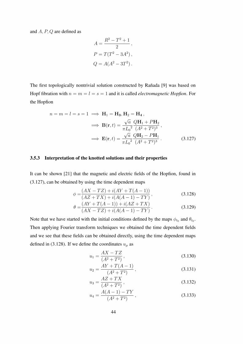
and A,P,Q are defined as

A =R2 − T 2 + 1

2,

P = T (T 2 − 3A2) ,

Q = A(A2 − 3T 2) .

The first topologically nontrivial solution constructed by Rañada [9] was based on

Hopf fibration with n = m = l = s = 1 and it is called electromagnetic Hopfion. For

the Hopfion

n = m = l = s = 1 =⇒ H1 = H3,H2 = H4 ,

=⇒ B(r, t) =

√a

πL02

QH1 + PH2

(A2 + T 2)3,

=⇒ E(r, t) =

√a

πL02

QH2 − PH1

(A2 + T 2)3. (3.127)

3.5.3 Interpretation of the knotted solutions and their properties

It can be shown [21] that the magnetic and electric fields of the Hopfion, found in

(3.127), can be obtained by using the time dependent maps

φ =(AX − TZ) + i(AY + T (A− 1))

(AZ + TX) + i(A(A− 1)− TY ), (3.128)

θ =(AY + T (A− 1)) + i(AZ + TX)

(AX − TZ) + i(A(A− 1)− TY ). (3.129)

Note that we have started with the initial conditions defined by the maps φt0 and θt0 .

Then applying Fourier transform techniques we obtained the time dependent fields

and we see that these fields can be obtained directly, using the time dependent maps

defined in (3.128). If we define the coordinates uµ as

u1 =AX − TZ(A2 + T 2)

, (3.130)

u2 =AY + T (A− 1)

(A2 + T 2), (3.131)

u3 =AZ + TX

(A2 + T 2), (3.132)

u4 =A(A− 1)− TY

(A2 + T 2), (3.133)

44

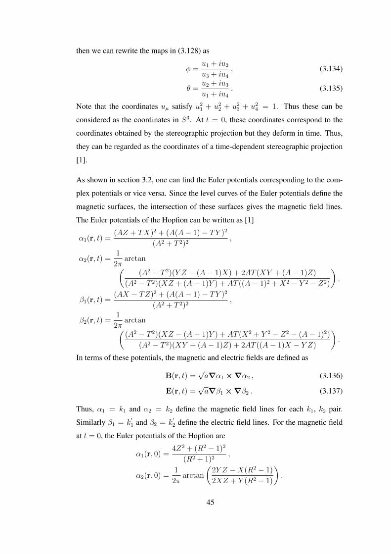
then we can rewrite the maps in (3.128) as

φ =u1 + iu2u3 + iu4

, (3.134)

θ =u2 + iu3u1 + iu4

. (3.135)

Note that the coordinates uµ satisfy u21 + u22 + u23 + u24 = 1. Thus these can be

considered as the coordinates in S3. At t = 0, these coordinates correspond to the

coordinates obtained by the stereographic projection but they deform in time. Thus,

they can be regarded as the coordinates of a time-dependent stereographic projection

[1].

As shown in section 3.2, one can find the Euler potentials corresponding to the com-

plex potentials or vice versa. Since the level curves of the Euler potentials define the

magnetic surfaces, the intersection of these surfaces gives the magnetic field lines.

The Euler potentials of the Hopfion can be written as [1]

α1(r, t) =(AZ + TX)2 + (A(A− 1)− TY )2

(A2 + T 2)2,

α2(r, t) =1

2πarctan(

(A2 − T 2)(Y Z − (A− 1)X) + 2AT (XY + (A− 1)Z)

(A2 − T 2)(XZ + (A− 1)Y ) + AT ((A− 1)2 +X2 − Y 2 − Z2)

),

β1(r, t) =(AX − TZ)2 + (A(A− 1)− TY )2

(A2 + T 2)2,

β2(r, t) =1

2πarctan((A2 − T 2)(XZ − (A− 1)Y ) + AT (X2 + Y 2 − Z2 − (A− 1)2)

(A2 − T 2)(XY + (A− 1)Z) + 2AT ((A− 1)X − Y Z)

).

In terms of these potentials, the magnetic and electric fields are defined as

B(r, t) =√a∇α1×∇α2 , (3.136)

E(r, t) =√a∇β1×∇β2 . (3.137)

Thus, α1 = k1 and α2 = k2 define the magnetic field lines for each k1, k2 pair.

Similarly β1 = k′1 and β2 = k

′2 define the electric field lines. For the magnetic field

at t = 0, the Euler potentials of the Hopfion are

α1(r, 0) =4Z2 + (R2 − 1)2

(R2 + 1)2,

α2(r, 0) =1

2πarctan

(2Y Z −X(R2 − 1)

2XZ + Y (R2 − 1)

).

45

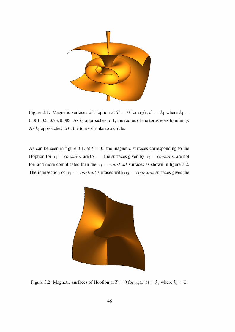
Figure 3.1: Magnetic surfaces of Hopfion at T = 0 for α1(r, t) = k1 where k1 =

0.001, 0.3, 0.75, 0.999. As k1 approaches to 1, the radius of the torus goes to infinity.

As k1 approaches to 0, the torus shrinks to a circle.

As can be seen in figure 3.1, at t = 0, the magnetic surfaces corresponding to the

Hopfion for α1 = constant are tori. The surfaces given by α2 = constant are not

tori and more complicated then the α1 = constant surfaces as shown in figure 3.2.

The intersection of α1 = constant surfaces with α2 = constant surfaces gives the

Figure 3.2: Magnetic surfaces of Hopfion at T = 0 for α2(r, t) = k2 where k2 = 0.

46

magnetic lines. If we imagine the intersection of these surfaces as depicted in figure

3.3, then we see that they will be closed curves on the surface of a torus, which are

topologically equivalent to circles. Since the Hopf index for the Hopfion is equal to

1, the magnetic field lines are circles, linked to each other only once. The set of all

these circles is called Hopf fibration [15].

If we consider the general case, we see that the field lines are knotted curves lying on

a torus. These knots are defined by two coprime integers (n,m), such that the curve

winds around a circle in the torus n times and the curve winds the line through the

hole of the torus m times [1]. Some of these torus knots can be seen in figure 3.4.

Since we have (n,m) and (l, s) torus knot solutions for the electromagnetic field,

we can analyze the properties of this class. Our initial construction was based on

decomposable fields that is E · B = 0. Let us see if this is valid for all knotted

Figure 3.3: Magnetic surfaces of Hopfion at T = 0 for α1(r, t) = 0.3 and α2(r, t) = 0

(left). The intersection of these surfaces, which are topologically equivalent to circles,

gives the magnetic field lines (right).

47

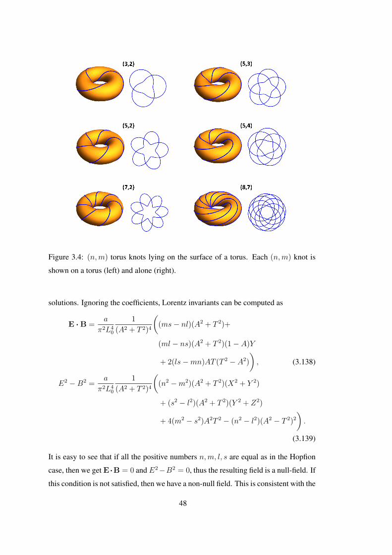
Figure 3.4: (n,m) torus knots lying on the surface of a torus. Each (n,m) knot is

shown on a torus (left) and alone (right).

solutions. Ignoring the coefficients, Lorentz invariants can be computed as

E ·B =a

π2L40

1

(A2 + T 2)4

((ms− nl)(A2 + T 2)+

(ml − ns)(A2 + T 2)(1− A)Y

+ 2(ls−mn)AT (T 2 − A2)

), (3.138)

E2 −B2 =a

π2L40

1

(A2 + T 2)4

((n2 −m2)(A2 + T 2)(X2 + Y 2)

+ (s2 − l2)(A2 + T 2)(Y 2 + Z2)

+ 4(m2 − s2)A2T 2 − (n2 − l2)(A2 − T 2)2).

(3.139)

It is easy to see that if all the positive numbers n,m, l, s are equal as in the Hopfion

case, then we get E ·B = 0 and E2−B2 = 0, thus the resulting field is a null-field. If

this condition is not satisfied, then we have a non-null field. This is consistent with the

48

observation (3.79). As a result, changing the (n,m), (l, s) values, we get a wider class

of knotted solutions for Maxwell equations which also covers the non-null fields.

If we compute the helicities of these knotted solutions

hm(t) =

∫d3rA ·B =

a

2

((nm+ ls) + (nm− ls)1− 6T 2 + T 4

(1 + T 2)4

), (3.140)

he(t) =

∫d3rC · E =

a

2

((nm+ ls)− (nm− ls)1− 6T 2 + T 4

(1 + T 2)4

). (3.141)

At the end of the section 3.4 we have seen that the Hopf indices of the two maps,

used to construct the magnetic and electric fields, should be the same for null fields.

Thus it is easy to understand that one should have mn = ls, which results in hm =

he = a(mn) for a null field as expected in (3.79). If we return to the general case, the

electromagnetic helicity can be written as

hem =hm + he

2= a(nm+ ls) . (3.142)

We see that hem is constant and does not change in time as we found in (3.74). If we

evaluate the magnetic and electric helicities as time goes to infinity, then we find

limt→∞

hm(t) = limt→∞

he(t) =a

2(nm+ ls) . (3.143)

We see that if the helicities of the magnetic and electric fields are not equal initially,

then they approach to the same value, the half of the electromagnetic helicity, in time.

Since we know from (3.142) that the sum of the helicities is constant, this means that

there is a helicity exchange between the magnetic and electric fields as in figure 3.5.

This is called exchange of helicities mechanism and was first studied in [22].

49

Figure 3.5: Evolution of the magnetic and electric helicities for n = m = 2 and

l = s = 1, where the helicities are represented in units of a. The dashed line with dots

represents the magnetic helicity and the dashed line represents the electric helicity. At

t = 0, hm = 4 and he = 1. As time passes, we can see the helicity exchange between

the magnetic and electric fields. However, the total electromagnetic helicity, which is

represented by the solid line, is equal to 5 and it does not change in time.

50

CHAPTER 4

CONCLUSIONS

In this work we have reviewed the set of torus knotted electromagnetic fields which

is proposed first by Rañada [9] and developed further by Arrayás, Bouwmeester and

Trueba [1]. Rañada construction is based on two complex scalars potentials φ and θ.

By imposing two conditions on these potentials, they are converted into maps from

S3 to S2. At some initial time t = 0, the magnetic and electric lines are given by

the level curves of complex maps φt0 and θt0 , respectively. Due to the topological

properties, Rañada used Hopf map for these complex maps. The first topologically

nontrivial solution constructed by Rañada [9] was based on Hopf fibration with n =

m = l = s = 1 and it is called electromagnetic Hopfion. For this particular case the

time dependent complex maps and the corresponding Euler potentials can be found.

Using the Euler potentials [1] of the Hopfion, we have analyzed the configuration

of magnetic field lines at t = 0. For the general case, magnetic (electric) lines are

(n,m) torus knots ((l, s) for electric field) and are linked to other magnetic (electric)

lines. It is shown that if n = m = l = s is satisfied, then the field is a null field

and the magnetic helicity is equal to the electric helicity initially, and does not change

in time. If n = m = l = s is not satisfied then the field is a non-null field and the

initial helicities are not equal to each other generally. If the initial helicities are not

the same, then it is shown that there is a helicity exchange between the magnetic and

electric fields. Due to the helicity exchange mechanism we see that the topological

structure of these field lines is not preserved. Since the helicity is related to the

difference of classical values corresponding to the number of right-handed and left

handed photons, a change in the helicity can be seen as an indication of creation or

annihilation of photons. Thus the process of helicity exchange and the change of the

topological structure should be understood in detail and it is an open problem.

51

52

REFERENCES

[1] M. Arrayás, D. Bouwmeester, and J. L. Trueba, “Knots in electromagnetism,”

Physics Reports, vol. 667, Nov 2016.

[2] M. Atiyah, “Geometry, Topology and Physics,” Quarterly Journal of the Royal

Astronomical Society, vol. 29, p. 287, Sep 1988.

[3] W. Thomson, “4. on vortex atoms,” Proceedings of the Royal Society of Edin-

burgh, vol. 6, pp. 94–105, 1869.

[4] K. F. Gauss, “Zur Mathematischen Theorie der Electrodynamischen Wirkun-

gen,” Königlichen Gesllschaft der Wissenschaften zu Göttingen, vol. 5, p. 605,

Sep 1877.

[5] P. A. M. Dirac, “Quantised singularities in the electromagnetic field,” Proceed-

ings of the Royal Society of London. Series A, Containing Papers of a Mathe-

matical and Physical Character, vol. 133, no. 821, pp. 60–72, 1931.

[6] Y. Aharonov and D. Bohm, “Significance of electromagnetic potentials in the

quantum theory,” Phys. Rev., vol. 115, pp. 485–491, Aug 1959.

[7] A. Trautman, “Solutions of the maxwell and yang-mills equations associated

with hopf fibrings,” International Journal of Theoretical Physics, vol. 16,

pp. 561–565, Aug 1977.

[8] A. F. Rañada, “A topological theory of the electromagnetic-field,” Letters in

Mathematical Physics, vol. 18, pp. 97–106, Aug 1989.

[9] A. F. Rañada, “Knotted solutions of the maxwell equations in vacuum,” Journal

of Physics A: Mathematical and General, vol. 23, pp. L815–L820, Aug 1990.

[10] A. F. Rañada and J. L. Trueba, “Topological electromagnetism with hidden

nonlinearity,” Modern Nonlinear Optics, Part III, Volume 119, Second Edition,

vol. 119, pp. 197 – 253, Mar 2002.

53

[11] G. Naber, Topology, Geometry and Gauge fields: Foundations. Texts in Applied

Mathematics, Springer New York, 2nd ed., 2010.

[12] L. H. Ryder, Quantum Field Theory. Cambridge University Press, 2nd ed.,

1996.

[13] T. T. Wu and C. N. Yang, “Concept of Nonintegrable Phase Factors and Global

Formulation of Gauge Fields,” Phys. Rev., vol. D12, pp. 3845–3857, 1975.

[14] C. Ehresmann, “Les connexions infinitésimales dans un espace fibré différen-

tiable,” in Séminaire Bourbaki : années 1948/49 - 1949/50 - 1950/51, exposés 1-

49, no. 1 in Séminaire Bourbaki, pp. 153–168, Société mathématique de France,

1952.

[15] H. Hopf, “Über die abbildungen der dreidimensionalen sphäre auf die

kugelfläche,” Mathematische Annalen, vol. 104, pp. 637–665, Dec 1931.

[16] A. F. Rañada, “On the magnetic helicity,” European Journal of Physics, vol. 13,

pp. 70–76, Mar 1992.

[17] T. Frankel, The Geometry of Physics: An Introduction. Cambridge University

Press, 3rd ed., 2011.

[18] J. H. C. Whitehead, “An Expression of Hopf’s Invariant as an Integral,” Pro-

ceedings of the National Academy of Sciences, vol. 33, no. 5, pp. 117–123,

1947.

[19] J. L. Trueba and A. F. Rañada, “The electromagnetic helicity,” European Journal

of Physics, vol. 17, pp. 141–144, May 1996.

[20] M. Arrayás and J. L. Trueba, “The method of fourier transforms applied to elec-

tromagnetic knots,” European Journal of Physics, vol. 40, p. 015205, Dec 2018.

[21] A. F. Rañada and J. L. Trueba, “Two properties of electromagnetic knots,”

Physics Letters A, vol. 232, pp. 25–33, Jul 1997.

[22] M. Arrayás and J. L. Trueba, “Exchange of helicity in a knotted electromagnetic

field,” Annalen der Physik, vol. 524, pp. 71 – 75, Feb 2012.

54