NEW K M C I -T PERIOD Rodrigo Caputo · discussants, Renzo Rossini and Raphael Bergoeing, and Sebastián Edwards, Douglas Laxton, Andrew Levin, David Rappoport, Claudio Soto, and

507

NEW KEYNESIAN MODELSFOR CHILE IN THE

INFLATION-TARGETING PERIOD

Rodrigo Caputo Central Bank of Chile

Felipe Liendo Chilectra

Juan Pablo Medina Central Bank of Chile

Dynamic stochastic general equilibrium (DSGE) models with nominal rigidities have become a popular tool for monetary policy analysis in recent years.1 The basic sticky price model has been enriched to include additional sources of nominal and real rigidities. These additional elements have been introduced to generate the observed degree of persistence in inflation, real wages, and output.2 Extensions of these closed economy models to open economies have highlighted the presence of the same types of rigidities.3

This paper was written while Felipe Liendo was affiliated with the Central Bank of Chile. The model presented in this paper is a simplified version of the DSGE model currently being developed at the Central Bank of Chile (the MAS project). We thank our discussants, Renzo Rossini and Raphael Bergoeing, and Sebastián Edwards, Douglas Laxton, Andrew Levin, David Rappoport, Claudio Soto, and Rodrigo Valdés for useful suggestions and comments.

1. Prominent examples of monetary business cycle models with price stickiness include Goodfriend and King (1997) and Rotemberg and Woodfoord (1997).

2. Altig and others (2004), Christiano, Eichenbaum, and Evans (2005), and Smets and Wouters (2003b) argue that these ingredients can indeed explain the joint dynamics of inflation, output, real wages, labor, consumption, investment, and nominal interest rates in the U.S. economy.

3. For new open economy models with nominal rigidities, see Adolfson and others (2005a, 2005b); Benigno and Benigno (2003); Galí and Monacelli (2005); Schmitt-Grohé and Uribe (2001), and Smets and Wouters (2003a).

Monetary Policy under Inflation Targeting, edited by Frederic Mishkin and Klaus Schmidt-Hebbel, Santiago, Chile. © 2007 Central Bank of Chile.

14.Caputo Liendo Medina 507-546.indd 01/03/2007, 18:19507

508 Rodrigo Caputo, Felipe Liendo, and Juan Pablo Medina

In this paper, we estimate a small open economy DSGE model for Chile to determine, at the aggregate level, the extent and magnitude of alternative sources of nominal and real rigidities to explain business cycles in Chile. Identifying the level of nominal and real rigidities that are present in the economy is a relevant step toward the efficient design of monetary policy. In particular, the existence (or absence) of certain rigidities may have very different implications for the trade-off between output and inflation stabilization that central banks face. For instance, standard new Keynesian models with nominal price rigidities and flexible wages generate a strong policy prescription: the role of monetary policy is to fully stabilize inflation. In this setup, inflation depends only on expected inflation and the gap between current output and its natural level (that is, the level that would prevail in the absence of nominal stickiness). In this framework, the central bank does not face a trade-off: stabilizing inflation is equivalent to stabilizing output from its natural level.

The absence of a trade-off between output and inflation stabilization is what Blanchard and Galí (2005) call the divine coincidence, and it is a controversial feature of the standard new Keynesian model. A frequently used approach to avoid this coincidence is to introduce a cost push shock to the new Keynesian Phillips curve, so the central bank faces a stabilization trade-off (see Clarida, Galí, and Gerler, 1999). This may seem an ad-hoc solution because, as noted by Blanchard and Galí (2005), conventional supply shocks do not appear as disturbances in the baseline new Keynesian model.

A more structural way of dealing with this coincidence is to remove the assumption that wages are flexible. Erceg, Henderson, and Levin (2000) find two important results when both wage and price decisions are staggered. First, the policymaker’s welfare function depends on the variance of output, price inflation, and wage inflation; second, it becomes impossible to set more than one variance to zero in the face of exogenous shocks. They thus demonstrate that, in contrast with the standard new Keynesian model with only price rigidities, there is a trade-off between stabilizing the output gap, price inflation, and wage inflation. In this case, the efficient equilibrium (the one under flexible prices and wages) cannot be reached with monetary policy.

The above result can be explained as follows. On the one hand, staggered wage setting can lead to cross-sectional dispersion in hours worked across households. This dispersion imposes a welfare cost because households dislike variations in their labor supply, given that they have an increasing marginal disutility of labor. The policymaker’s


509New Keynesian Models for Chile in the Inflation-Targeting Period

welfare function thus depends not only on the variance of output and inflation (as in the standard new Keynesian model with only price rigidities), but also on the variance of wage inflation, which is directly correlated with the variance of employment. The variances of output, price inflation, and wage inflation have a negative weight on the policymaker’s welfare function. On the other hand, the fact that wages are staggered implies that marginal costs depend not only on the output gap, but also on the difference between the observed real wage and the equilibrium real wage (see Blanchard and Galí, 2005). As a consequence, the New Keynesian Phillips curve is a function of both the output and real wage gap. In this context, any shock that moves the equilibrium real wage generates a movement in price inflation (because the observed real wage cannot fully adjust toward its equilibrium level). This movement can only be offset by altering the output gap. Therefore, when both wage and price stickiness are introduced, the divine coincidence no longer holds, and there is a trade-off between stabilizing price inflation and output. In contrast with the ad-hoc supply shocks that are usually introduced to generate a trade-off between price inflation and output gap stabilization, in this case this trade-off arises endogenously.

Blanchard and Galí (2005) consider real rigidities, such as wage indexation, in addition to nominal rigidities, such as price and wage stickiness. In this case, the existence of a stabilization trade-off will depend on both the degree of wage inertia and the nominal rigidities.

A policy rule that seeks to fully stabilize inflation is clearly suboptimal in the presence of wage rigidities. In particular, it can exacerbate the volatility of both output and wage inflation. In this case, an alternative policy rule that seeks to minimize the volatility of a weighted average of wage and price inflation may perform better, as shown by Erceg, Henderson, and Levin (2000) and Blanchard and Gal (2005). In other words, optimal policy prescriptions depend on the set of frictions that the economy faces and, in particular, the importance of nominal and real rigidities in the wage setting process.4

Standard reduced-form models, with no explicit microeconomic foundations, are unable to identify, in practice, the source of nominal

4. Additional examples of optimal monetary policy with sticky prices and one or more nominal or real frictions include Adão, Correia, and Teles (2003); Benigno and Woodford (2004); Kahn, King, and Wolman (2003); Lama and Medina (2004); Schmitt-Grohé and Uribe (2004, 2005); and Woodford (2001).



and real frictions. Their contribution to policy analysis is thus rather limited. We lay down a structural model containing both nominal and real frictions and estimate it for Chile. The model features habit formation in the consumer’s utility function, introduces wage and price rigidities, and allows for the possibility of imperfect exchange rate pass-through to import prices. We also explore alternative specifications for the monetary policy reaction function, assessing whether the central bank has reacted to expected, contemporaneous, or past inflation. Finally, we also conduct a subsample analysis to determine whether any of the relevant rigidities or policy coefficients changed after 1999, when full-fledged inflation targeting and a free-floating exchange rate regime were introduced.

We use Bayesian techniques to estimate the model. To apply this methodology we combine priors and the likelihood function to obtain the posterior distribution of structural parameters. The likelihood function of the parameters is evaluated using the Kalman filter of a log-linear approximation of the model. We use the Metropolis-Hastings algorithm to approximate the posterior distribution.

We adopt a Bayesian approach for various reasons.5 First, the Bayesian approach is system-based and fits the dynamic stochastic general equilibrium model to a vector of time series. Second, the estimation is based on the likelihood function generated by the DSGE model, rather than, for instance, the discrepancy between DSGE model responses and vector autoregression (VAR) impulse responses. Third, prior distributions can be used to incorporate additional information into the parameter estimation. Fourth, this approach can cope with potential model misspecification and possible lack of identification of the parameters of interest. In a misspecified model, if the likelihood function peaks at a value that is at odds with the prior information on any given parameter, the posterior probability will be low. The prior density thus allows us to weight information about different parameters according to its reliability. Lack of identification, in turn, may result in a likelihood function that is flat for some coefficient values. Hence, based on the likelihood function alone, it would not be possible to identify the value of the parameters of interest. The Bayesian approach copes with this problem by introducing prior distributions. In fact, a proper prior can introduce curvature into the objective function, the posterior distribution, making it possible to identify the value of

5. See Fernández-Villaverde and Rubio-Ramírez (2004) and Lubik and Schorfheide (2006) for a deeper discussion of the advantages of this approach.



different parameters. Finally, as pointed out by Fernández-Villaverde and Rubio-Ramírez (2004) and Rabanal and Rubio-Ramírez (2005), Bayesian estimation delivers a form for comparing models through, the marginal likelihood. This makes it possible to determine the extent to which additional ingredients of the model help explain the Chilean data. An advantage of using the marginal likelihood to compare models is that it penalizes overparametrization.

In recent years, several macroeconometric models with Keynesian features—for example, a Phillips curve—have been estimated for the Chilean economy to analyze monetary policy.6 The parameters estimated in this type of model do not have a structural interpretation, however, since they are based on reduced-form equations. In this paper, the parameters estimated do have a structural interpretation. Céspedes, Ochoa, and Soto (2005) similarly estimate a structural Phillips curve for Chile, derived from a new Keynesian model similar to ours. Nevertheless, they make a single equation estimation of that Phillips curve, which can still suffer from identification problems because it does not take into account the cross-correlation between inflation and the rest of the equations in the system.7 Other studies use general equilibrium models for the Chilean economy, in which the parameters have a structural interpretation. However, the values of the parameters in these models are calibrated and not estimated.8 Moreover, these models do not consider nominal rigidities such as those emphasized by the new Keynesian literature. Caputo and Liendo (2005) estimate a general equilibrium model for Chile based on Galí and Monacelli (2005), where wages are fully flexible and aggregate consumption is completely smooth.9 This model also lacks the imperfect pass-through to imported prices considered here.

Our main results are as follows. First, models with both price and wage rigidities fit better the Chilean data. Rabanal and Rubio-Ramírez (2005) highlight the presence of both staggered prices and wage setting as salient features for explaining U.S. data. They also

6. See Corbo and Tessada (2005); García, Herrera, and Valdés (2002); García and others (2005); and Medina and Valdés (2002). Gallego, Schmidt-Hebbel, and Servén (2005) develop a general equilibrium model derived from first principles, but in which some equations (such as the labor supply) are reduced form and not fully consistent with the rest of the model.

7. See Leeper and Zha (2000) for a discussion of identification problems in the estimation of reduced-form equations or partial equilibrium models.

8. See, for example, Bergoeing and Soto (2005); Duncan (2005).9. This last result is due to the fact that the model displays perfect risk sharing in

international financial markets and does not incorporate habit in consumption.



show that the point estimates of price rigidity are higher than those of wages in the U.S. economy.10 In our case, the degree of rigidity is higher for wages than for prices. Our estimation shows that nominal wages are optimally adjusted every three quarters, on average, while the optimal horizon for price adjustments is every two quarters. The subsample analysis suggests that both prices and wages were adjusted less frequently after 1999 than before. This result is in line with Céspedes and Soto (in this volume), who find that a highly credible inflation-targeting regime leads to less frequent price adjustments. Another relevant feature of the Chilean economy is the imperfect pass-through from the exchange rate to import prices. Our results indicate that import prices are kept fixed for around two years, on average, with a degree of stickiness that does not change over time.

Second, adding wage indexation clearly improves the fit of the model. This level of indexation is comparatively larger than that of domestic and import prices. Wage indexation generates a more persistent response of inflation to shocks, and makes inflation fluctuations more costly in terms of output and labor.11 It is also, as mentioned above, one of the determinants of the monetary policy trade-off.

Third, real rigidities such as habit formation also deliver a better account of the aggregate data, although the estimated values are quantitatively small. Chari, Kehoe, and McGrattan (2000) point out that models with nominal rigidities do not generate enough persistence in output following a monetary shock as predicted by semi-structural VARs in U.S. The inclusion of habit formation in consumption has helped solve this issue.12 In the case of Chile, our work confirms the relevance of this type of real rigidity to explain business cycle fluctuations.

Fourth, models with a Taylor rule that reacts to expected inflation better characterize the monetary policy in the sample period. As found by Corbo (2002), Schmidt-Hebbel and Tapia (2002), and Caputo (2005), the policy response to inflation is comparatively larger than the response to output and to exchange rate. On the other hand, the subsample analysis indicates that the degree of interest rate smoothness increased after 1999, while the response to inflation relative to output became less aggressive. This result may be an

10. The calibrated values used by Christiano, Eichenbaum, and Evans (2005) suggest that wages are slightly stickier than prices.

11. See Jadresic (2002).12. See Fuhrer (2000).



indication that, in a context of greater policy credibility, the inflation target can be achieved with a lower sacrifice ratio.

The rest of the paper is organized as follows. Section 1 describes the structure of a dynamic general equilibrium model for the Chilean economy. Section 2 then explains the econometric strategy to estimate the parameters and compare models. In this section, we also describe the data used and our choice of priors and calibrated parameters to construct the posterior distribution. In section 3, we present the results of the Bayesian estimation. Finally, section 4 concludes.

1. A SIMPLE SMALL OPEN ECONOMY MODEL

In this section, we describe a dynamic stochastic general equilibrium (DSGE) model with nominal and real rigidities. This microfounded model is closely related to the new open economy literature. It is a simplified version of Medina and Soto’s (2005) model for the Chilean economy, but to make this paper self-contained, we subsequently describe the structure of the model and the decision problems of the agents.

In this setup, the domestic economy is open to international markets, and it is small for the rest of the world. The last assumption implies that international prices, foreign interest rates, and foreign demand are not affected by domestic agents. The main rigidities of the baseline model are the following: sticky prices and wages, past inflation indexation of prices and wages, and habit formation in consumption. Home goods are sold to domestic and foreign households. We also assume that these goods are an imperfect substitute of the foreign (imported) good.

The economy includes two types of firms: intermediate goods producers and retailers. The first type produces differentiated varieties of intermediate goods. For simplicity, we assume that labor is the only variable input used for production. These firms have monopolistic power over the variety of goods they produce. The second type of firms are competitive retailers that combine intermediate goods to produce home goods.

Households supply a differentiated labor service and receive the corresponding wage compensation. Each household has a monopolistic power over the type of labor service it provides. Furthermore, households are the owners of firms producing intermediate goods, so they receive the income corresponding to the monopolistic rents generated by these firms.



Monetary policy is modeled as a Taylor-type rule that incorporates interest rate inertia. In particular, the interest rate reacts to inflation, GDP growth, and its own lagged value. The rule is augmented to include a response to nominal exchange movements. We also test whether the data support a reaction to expected, contemporaneous, or past inflation.

We assume that labor productivity grows at a rate gy. Finally, we also assume that in the steady state, the inflation rate is exogenously determined by the monetary authority, and it is nonzero.

1.1 Households

The domestic economy is inhabited by a continuum of households indexed by j ∈ [0, 1]. The expected present value of the utility of household j is given by:

E C j b g Cl j

tt y t t

tL

0

1

11

β ζ

σ

log ( )− +

−

( )

+

+

σσϖ

L

t

t

u

t u

M j

P+

+( )

+

= 1

1

0

∞∞

∑ , (1)

where lt(j) is labor effort, Ct(j) is total consumption, and Mt(j) corresponds to the total nominal balances held at the beginning of period t. The inverse elasticity of labor supply with respect to real wages is represented by σL, while ζt is a preference shock that shifts the labor supply. The ϖ coefficient represents the importance of real balances, Mt( j )/Pt

in the utility function. Preferences display habit formation, measured by the parameter b. The consumption good is a composite of home and imported goods:

C j C j C jt H t F t( )= −( ) ( )

+ ( )

−( ) −( )1 1 1 1 1

α αη η η η η η

, ,

−( )η η 1

, (2)

where η is the elasticity of substitution between home and imported goods, and α is the share of imported goods in the domestic consumption basket. For any level of consumption, each household purchases a composite of home and imported goods in period t to minimize the total cost of its consumption basket. Each household thus minimizes PH,tCH,t(j) + PF,tCF,t(j), subject to equation (2), where PH,t and PF,t are the price of home and imported goods, respectively. Therefore, the demand for home and imported goods are given by



CP

PCH t

H t

tt,

,= −( )

−

1 αη

; CP

PCF t

F t

tt,

,=

−

αη

(3)

The price of the consumption good is defined as

P P Pt H t F t= −( ) +

− − −( )1 1 1 1 1

α αη η η

, , . (4)

We detrend and log-linearize expressions (3) and (4) to obtain the following:13

c c p pHt t Ht t , ,= − −

η , (log 1)

c c p pFt t Ft t , ,= − −

η , and (log 2)

p p pt Ht Ft = −

+

1 α α, , . (log 3)

Domestic households have access to three different types of assets: money, Mt(j); one-period noncontingent foreign bonds, Bt*(j); and one-period domestic contingent bonds dt+1(j), which pay out one unit of domestic currency in a particular state. There are no adjustment costs in the portfolio composition. However, each time a domestic household borrows from abroad, it must pay a premium over the international price of external bonds. This premium is introduced in the model to obtain a well-defined steady state for the economy.14 The household budget constraint is thus given by

PC j E q d je B j

ie B

t t t t t tt t

tt t

( )+ ( )

+

( )

+

+ +,

*

*1 1

1 Θ**

,

*

P X

M j

W j l j d j e B j M

X t t

t

t t t t t

+ ( )=

( ) ( )+ ( )+ ( )+−1 tt t tj T− ( )+ +1 Π ,

(5)

where Πt are profits received by domestic firms, et is the nominal exchange rate, Wt(j) is the nominal wage set by household j, and Tt represents per capita lump-sum net transfers from the government.

13. Lowercase variables with ˆ denote log-linear deviation with respect to the steady-state values.

14. See Schmitt-Grohé and Uribe (2003) for different ways to achieve a steady state that is independent of initial conditions in small open economy models.



The term

Θe B

P Xt t

X t t

*

,

corresponds to the premium domestic households have to pay each time they borrow from abroad, where

B B j djt t* *= ( )∫0

1

is the aggregate net foreign asset position of the economy and PX,tXt is the nominal value of exports.15 Also, qt,t+1 is the price of domestic contingent bonds in period t, normalized by the probability of the occurrence of the state. Assuming the existence of a full set of contingent bonds ensures that the consumption of all households is the same, independently of the labor income they receive each period.16

Our assumption that the premium depends on the aggregate net foreign asset position of the economy implies that households take Θ(∙) as given when deciding their optimal portfolios. In other words, households do not internalize the effect on the premium of changes in their own foreign asset position. In the steady state, the Θ(∙) function is parameterized as

Θ ΘeBP XX

*

= and ′( )

( )=

Θ

Θ

eB P X

eB P X

eBP X

X

X X

*

*

*

µ .

Here B*corresponds to the steady-state net foreign asset position, while PX X is the steady-state value of exports. When the country as a whole is a net debtor, µ is the elasticity of the upward slopping supply of international funds.

Consumption and saving decisions

Households choose consumption and the composition of their portfolios by maximizing equation (1) subject to equation (5). The optimal conditions can be combined to obtain log-linear expressions for the Euler equation and the uncovered interest parity condition:

15. Since the economy is growing in the steady state, the net asset position is also growing in the long run. Therefore, to have a stationary risk premium, this premium must be a function of the ratio of the net asset position and some variable that grows at the same rate in the steady state. We chose exports, since they could represent a form of international collateral (see Caballero and Krishnamurthy, 2001)

16. This, in turn, motivates the exclusion of index j in expressions (log 1) and (log 2).



cb

E cb

bc

bb

i Et t t t t t t =

+

+

+−

−+

−+ − +

11 1

111 1 1π̂

and (log 4)

i i E e rer b p pt t t t t t X t t = +

+ + − −

+

* *,∆

1µ −

xt , (6)

where et is the nominal exchange rate and rer e p pt t Ft t

= + −,* is the

real exchange rate (both measured as the log deviation from their steady-state values). Based on the real exchange rate definition, the nominal exchange rate devaluation can be defined as

∆e rer rert t t t t = − − +−1 π π*

, (log 5)

where π t* is foreign inflation (in foreign currency).

Labor supply decisions and wage setting

Each household j is a monopolistic supplier of a differentiated labor service. There is a set of perfectly competitive labor service assemblers that hire labor from each household and combine it into an aggregate labor service unit, lt, that is then used by the intermediate goods producer. The labor service unit is defined as follows:

l l j djt tL L

L L

= ( )

−( )−( )

∫ε ε

ε ε1

0

1 1

. (7)

where εL is the elasticity of substitution of different types of labor. The optimal composition of this labor service unit is obtained by minimizing its cost, given the different wages set by different households. In particular, the demand for the labor service provided by household j is:

l jW j

Wlt

t

tt

L

( )=( )

−ε

, (8)

where Wt(j) is the wage rate set by household j and Wt is an aggregate wage index defined as

W W j djt tL

L

= ( )

−−( )

∫1

0

1 1 1ε

ε

. (9)



Following Erceg, Henderson, and Levin (2000), we assume that wage setting is subject to a nominal rigidity à la Calvo (1983). In each period, each household faces a constant probability (1 – φL) of being able to re-optimize its nominal wage. We assume there is an updating rule for all households that cannot re-optimize their wages. In particular, if a household cannot optimize during i periods between t and t+i, then its wage at time t+i is given by

W j W jt i W ti

t+ ( )= ( )Γ , , (10)

where ΓW ti

, describes an adjustment rule for wages, which is defined as

ΓW ti

t j t j yj

iL L g, .= +( ) +( ) +( )+ − +

−

=∏ 1 1 11

1

1π π

ξ ξ

This “passive” adjustment rule implies that workers who do not optimally reset their wages update them by considering a geometric weighted average of past CPI inflation and the inflation target set by the authority, πt . The inclusion of (1 + gy) in the above expression prevents large real wage dispersion along the steady-state growth path. Once a household has decided on a wage, it must supply any quantity of labor service that is demanded at that wage. A particular household j that is able to re-optimize its wages at time t solves the following problem:

max ,,

W jt L

it t i

t W ti

t ii

t t i

t

EW j

P

l j

( )+

+=

∞

+

=( )

− ( )

∑φ

ζ

ΛΓ

0

− +( )

( )+ + − +

σL C b g C l jt i y t i t i1 1 ,

subject to the labor demand (equation 8) and the updating rule for the nominal wage (equation 10). The variable Λt,t+i is the relevant discount factor between periods t and t+i; it is given by

Λt t ii t y t

t i y t i

C b g C

C b g C, +

−

+ + −

=− +( )

− +( )β

11

1

1

.

Combining the optimal choice of wages with the updating rule and the definition of the aggregate real wage, we obtain the following log-linear expression for real wages, wr:



11 1 1

1+

+ +( )

= −( ) −( ) +−

ν φ

σ ε φ νν φ σ

L L

L L L Lt L L L t twr l

bc −−

−+

+ +( ) + +( )

−

−

bb

c

wr E w

t t

L L L t L L L t

1

1 1

1

1

ζ

σ ε φ σ ε ν rrt

L L L L L t L L L L t

L L L

+

−

( )

− +( ) +( ) + +( )

+ +( )

1

11 1

1

σ ε φ ν ξ π σ ε φ ξ π

σ ε ν EEt tπ +( )1 ,

(log 6)

where νL = βφL

1.2 Home Goods Sector

There are two types of firms in this sector: retailers and intermediate goods producers. The latter use labor to produce a differentiated good while the former combine these intermediate inputs to produce the home good consumed by domestic and foreign households.

Retailers

Retailers create units of home goods according to a constant-elasticity-of-substitution aggregator of a continuum of intermediate products that are indexed on the unit interval, zH ∈ [0, 1]. Specifically, retailers produce YH,t units of home goods using the following constant-return-to-scale technology:

Y Y z dzH t H t H HH H

H H

, ,= ( )

−( )−( )

∫ε ε

ε ε1

0

1 1

(11)

Retailers then allocate their demands for intermediate goods by minimizing the total cost of production, subject to equation (11), where. εH is the elasticity of substitution of differentiated intermediate goods. The optimal combination of intermediate goods determines a demand for each variety, zH:

Y z YP z

PH t H H tH t H

H t

H

, ,,

,( )=

( )

−ε

, (12)

where PH,t(zH) is the price of the variety zH and PH,t is the aggregate price level of home goods, which is given by



P P z dzH t H t H HH

H

, ,= ( )

−−( )

∫1

0

1 1 1ε

ε

. (13)

The total production of home goods is consumed by domestic and foreign households. The foreign demand for home goods is given by the following expression, in log-linear form:

c c p p rerHt t Ht t t ,

* * *,= − −

−

η , (log 7)

where c* is the aggregate level of foreign consumption and η* is the elasticity of substitution of the foreign demand.

Intermediate goods producers

The producers of intermediate home inputs are assumed to be monopolistic competitors. We further assume that they face a nominal rigidity that prevents them from adjusting prices optimally in every period. For simplicity, we assume that the only variable input is labor. The production function can thus be expressed as follows:

Y z A g l zH t H H t y

t

t H, ,( )= +( ) ( )1 , (14)

where AH,t is a productivity shock. The cost of producing is Wtlt(zH), which implies that the marginal cost of each intermediate firm is equal to Wt/[AH,t(1 + gy)t].

Following Calvo (1983), we assume that firms adjust their prices infrequently. In particular, they do so when receiving a signal. In every period, the probability of receiving a signal and adjusting prices is 1 – φH for all firms, independent of their history. If the firm does not receive a signal, then it follows a simple updating rule defined by the function ΓH t

i, . Thus, if a firm, zH, receives a signal in period t,

then it will adjust the price of its variety, PH,t(zH), so as to maximize the following expression:

max,

,

, , ,

P zt H

it t i

i

H ti

H t H t H t y

t

H t H

E

P z W A g

( )+

=

∞

( )

×( )− +( )

∑ φ Λ

Γ

0

1

( )+

+PY z

t iH t i H, , (15)



subject to the restrictions imposed by the technology and considering the demand the firm faces for its variety (equation 12). The passive adjustment rule is given by

ΓH ti

H t jj

i

t jH H

, ,= +( ) +( )+ −=

+

−

∏ 1 111

1π π

ξ ξ , (16)

where 1 + πH,t = (PH,t/PH,t–1) , and where πt j+ corresponds to the inflation target set by the authority. Relative price changes may have a feedback impact through this adjustment rule. Firms that do not optimally adjust take into consideration the inflation target, which is set in terms of consumption goods inflation. The parameter ξH captures the degree of indexation in the economy. The larger this parameter, the larger is the weight of past inflation in defining new prices.

Combining the optimal price setting with the automatic updating rule yields a hybrid Phillips curve for home goods inflation:

πββξ

πξ

βξπ

φ βφ

Ht

Ht Ht

H

HHt

H H

E, , ,=+

+

+

+−( ) −

+ −1 11 1

1 1

(( )+( )

+ − −

φ βξH H

t t Ht Htwr p p a1

, , . (log 8)

1.3 Imports

The import sector consists of a continuum of firms that buy a homogeneous good in the foreign market. These firms turn the imported good into a differentiated import.17 Competitive assemblers combine this continuum of differentiated imports in a final imported good, YF. The technology of importing assemblers is given by

Y Y z dzF t F t F FF F

F F

, ,= ( )

−( )−( )

∫ε ε

ε ε1

0

1 1

,

where εF is the elasticity of substitution of differentiated import goods and YF,t(zF) is the quantity of a differentiated import, zF, used by the assemblers. The optimal mix of the differentiated import is given by the following demand:

17. This differentiating technology can be interpreted as product branding.



Y z YP z

PF t F F tF t F

F t

F

, ,,

,( )=

( )

−ε

, (17)

where PF,t(zF) is the price of the import brand, zF, charged in the domestic market, and PF,t is the aggregate price of imported goods in the domestic market:

P P z dzF t F t F FF

F

, ,= ( )

−−( )

∫1

0

1 1 1ε

ε

.

The different importing firms buy the homogeneous foreign good abroad at price PF t,

* , in foreign currency. Each importing firm possesses monopoly power over the domestic retailing of its variety. We assume local currency price stickiness to allow for incomplete exchange rate pass-through to the import prices. An importing firm adjusts the domestic price of its variety infrequently, when receiving a signal. The signal arrives with probability 1 – φF each period. The arrival of the signal is independent of the history of a particular firm and identically distributed across importing firms. As in the case of domestically produced goods, if a firm does not receive a signal, it updates its price following a passive rule. This passive rule is defined through Γi

F,t and states that if an importer, zF, does not receive a signal to optimally adjust its price between time t and t + i, then its price at time t + i is given by Γi

F,tPF,t(zF). The updating rule is defined as

ΓiF t t i F t j t j

j

iF F

, , ,+ + − +

−

=

= +( ) +( )∏ 1 111

1π π

ξ ξ ,

where 1 + πF,t = PF,t/PF,t–1. Hence, when a generic importing firm, zF, receives a signal, it

chooses a new price by maximizing the following expression:

max,

,, , , ,

*

P zt F

i

it t i

F t t i F t F t i F t i

f t F

EP z e P z

( )=

∞

++ + +( )

( )−∑ φ

0Λ

Γ FF

t iF t i FP

Y z( )

( )

+

+,,

subject to the domestic demand for variety zF (equation 17) and the updating rule. As in the case of home goods, the optimal price setting can be combined with the automatic updating rule to obtain a Phillips curve for the inflation of imported goods in the domestic market:



ˆ ˆ ˆ, , ,

πββξ

πξ

βξπ

φ

F tF

t F t

F

FF t

F

E=+

+

+

+−( )

+ −1 1

1

1 1

111

−( )+( )

+ −

βφφ βξ

F

F Ft F t F t

e p pˆ ˆ ˆ .,

*,

(log 9)

1.4 Monetary Policy

We assume that monetary policy in Chile could be modeled as a Taylor-type rule:

r r y et i t i t y t e t tm = + −( ) + +( )+−ψ ψ ψ π ψ ψ νπ1 1 ˆ ˆ ∆ ∆ (log 10)

To be consistent with monetary policy in Chile during the sample period analyzed, we consider the real interest rate, rt , as the monetary policy instrument. In this specification, ψπ and ψy are, respectively, the long run responses of the monetary authority to deviations of inflation and GDP growth from their target levels (steady-state values). We also include a reaction to the nominal devaluation, ψ∆e, to analyze empirically whether this feature is relevant for Chile. Finally, ψi controls for the degree of interest rate smoothing, which has been proved to be important for explaining monetary policy empirically.

This specification has been estimated for Chile in several papers, including Schmidt-Hebbel and Tapia (2002), Caputo (2005), Parrado and Velasco (2002), and Corbo (2002). The evidence generally supports the existence of a Taylor-type policy reaction function that responds to inflation deviations from target, to output, and to real exchange rate misalignments. The papers cited above perform their estimations in a univariate setting. In this paper, the policy rule coefficients are estimated along with the rest of the coefficients that characterize the economy. This allows us to exploit cross-equation restrictions that link agents’ decision rules to the policy parameters.

Finally, the real (ex-ante) and nominal interest rates are linked through the following identity:

r i Et t t t = −

+π 1

(log 11)



1.5 Aggregate Equilibrium

Using the aggregate equilibrium in the labor market, we can write the market-clearing condition for the home goods sector as,

a lCY

cCY

cH t tH

H

H tH

H

H t , , ,

*+ =

+ −

1 , (log 12)

where CH/YH is the steady-state fraction of home goods production that is consumed by domestic households.18

Total GDP is given by

Y C P X e P Ct t X t t t F t F t= + −, ,*

, .

PX,tXt is the total level of exports, which is given by,

P X P C XX t t H t H t S t, , ,*

,= + ,

where XS,t is the level of commodity exports, which represents a significant share of Chilean exports. We treat this component of exports as exogenous and stochastic.19 We log-linearize the GDP around the steady-state growth path to get

yNXY

cCY

cXY

CYt t

HHt

H = −

+

+ −

1

*

,*

*

− −

x

NXY

cSt Ft

, ,α 1 , (log 13)

where NX/Y is the net exports-to-GDP ratio. The detrended and log-linearized expression for exports is

ˆ ˆ ˆ ˆ,

*

, ,*

*

p xCX

p cCXX t t

HH t H t

H+ =

+( )+ −

1

ˆ .,xS t (18)

18. We do not need to specify the money market equilibrium condition since money is separable in the utility function and the policy instrument is the interest rate.

19. In Chile commodities represent a significant share of total exports. These commodities are produced independently of domestic economic conditions (the interest rate, real wages, and so forth) and they can therefore be considered as exogenous in the short run.



Using this expression for exports, we can write the uncovered interest parity (equation 6) as follows:

ˆ ˆ ˆ ˆ* **

i i E e rer bCY

YXt t t t t

H= + ( )+ +

−

+∆ 1 µ

− +

− −

ˆ ˆ ˆ, ,*

*

p p c

CY

H t t H t

H1 YYX

xt

ˆ . (log 14)

Since we model an open economy, the net foreign asset evolution is governed by (log-linear form)

1

1

1 1

11 1−

+

=

−−

+ +

µ µ

πibt

gy*

*ˆ*Θ ++

−

+

i

MY

YeB

rert*

*Θ

1

1 ++

++

+

−−

ii

gbt

y

t*

*

*

*ˆ ˆ ˆΘ

1

1 11

ππtt

H HCY

YeB i

CY

*

*

**

*

+

−

+

µ

1 Θ

× − +

YX

p p cH t t H tˆ ˆ ˆ, ,**

*

**

+ −

−+

−XY

CY

YeB i

H µ

11

Θ

CCY

YX

xMY

Y

H

S t

*

,ˆ

× −

eeB

cF t* ,ˆ .

(log 15)

To close the model, we link the change in the real price of home and imported goods with consumption price inflation, as follows:

p p p pHt t Ht t Ht t

, , ,− = − + −− −1 1 π π , and (log 16)

p p p pFt t Ft t Ft t

, , ,− = − + −− −1 1 π π . (log 17)



1.6 Stochastic Exogenous Process

The economy is subject to seven orthogonal fluctuations: a labor supply shock ( ζ t ); a foreign interest rate shock ( it

* ); a foreign inflation shock ( π t

* ); a foreign demand shock ( ct* ); a productivity shock ( aHt

, ); a monetary policy shock ( νt

m ); and a commodity export shock ( xSt , ). We

specify the following stochastic processes for these shocks:

ζ ρ ζ εζ ζ

t t t= +−1 , (log 18)

i it i t i t * *

,* *= +−ρ ε1 (log 19)

π ρ π επ π

t t t

* *,* *= +

−1 (log 20)

c ct c t c t * *

,* *= +−

ρ ε1 (log 21)

a aHt a Ht at , , ,= +−ρ ε1 (log 22)

ν εtm

m t= , (log 23)

x xSt S St St , , ,= +−ρ ε1 (log 24)

where each innovation εi,t follows a normal distribution with zero mean and variance σi t,

2 , for i = ζ, i*, π*, c*, a, m, S, and innovations are uncorrelated with each other.

1.7 Alternative Models

We consider alternative models that reduce the degree of rigidity and modify the specification of the monetary policy rule. In addition to the baseline case, we estimate five models that remove, one by one, some of the nominal and real rigidities for a given policy rule. The first alternative model, M1, removes the assumption that there is incomplete exchange rate pass-through to the import prices; it therefore considers φF = ξF = 0. The second model, M2, removes the assumption of price indexation of home goods, in addition to incomplete pass-through. That is, in this model, φF = ξF = ξH = 0. The third alternative model, M3, further removes wage indexation, such that φF = ξF = ξH = ξL = 0. In this case, inflation is not inertial, and



wages are not indexed to past inflation. The fourth model, M4, removes the assumption that wages are sticky. This means that φL = 0, so workers set their wages optimally in each period. As before, φF = ξF = ξH = ξL = 0. In this specification, there is no inertial behavior in the inflation equation or in the wage equation. Finally, model M5 assumes no habit formation in the consumers’ utility function. As a result, in this specification, b = 0 and φF = ξF = ξH = ξL = φL = 0. This last case is the standard new Keynesian model with no inertia (inflation and consumption are forward looking) and sticky prices.

For the baseline model (which takes into account the nominal and real rigidities of the economy), we investigate how monetary policy has reacted in the inflation-targeting period. In so doing, we follow Lubik and Schorfheide (2006) and assess the plausibility of alternative policy rule specifications. We are interested in determining what inflation horizon is implicit in the policy reaction function. In particular, we test whether the Central Bank of Chile has been forward- or backward-looking with regard to inflation. In the first case, we modify equation (log 10) by replacing current inflation,π t , with expected one-period-ahead inflation, Et tπ +( )1 . In the second case, the target is one-period-past inflation, π t−1 .

To compare alternative model specifications, we use the Bayes factor, which enables us to assess which model is more likely to generate the data.

2. ECONOMETRIC METHODOLOGY

Having set up a theoretical model with nominal and real rigidities, we estimate the structural coefficients that characterize the economy. As a previous step, we kept a number of parameters fixed throughout the estimation procedure. Most of these parameters can be related to the steady-state values of the observed variables in the model, and they are therefore calibrated so as to match some long-run statistics. We assume an annual long-run labor productivity growth of 3.5 percent.20 The long-run annual inflation rate is 3 percent, which is consistent with the target value defined by the Central Bank of Chile in 2001. The subjective discount factor,β, is set close to 0.99 (annual basis) to yield an annual nominal interest rate of 7.0 percent in the steady state. The share of imported goods

20. This is consistent with 5 percent long-run GDP growth and 1.5 percent labor force growth.



in the consumption basket,α, is set at 40 percent, while the share of home goods production in total GDP, YH/Y, is set at 90 percent.21 The ratio of net exports to GDP, NX/Y, in the steady state is equal to 2.0 percent, which is consistent with the average value of this statistic in the sample period analyzed. The remaining shares can be obtained using these values and the steady-state relations (see the appendix). Obtaining direct information on price and wage markups is cumbersome, so we use values in the range used by other studies: εL = εH = εF = 9.22

We can now estimate the remaining coefficients that characterize the economy. In particular, we want to know the values of θ = (σL, b, φH, φL, φF, η, η*, µ, ξL, ξH, ξF, ψi, ψπ, ψy, ψ∆e, ρζ, ρi*, ρπ*, ρc*, ρa, ρs, σζ, σi*, σπ*, σc*, σa, σs). We follow Rabanal and Rubio-Ramírez (2005), Lubik and Schorfheide (2006) and Adolfson and others (2005b) in using Bayesian estimation techniques for both the model estimation and our evaluation.

Simply stated, the Bayesian approach works as follows. First, it places a prior distribution with density p(θ) on the structural parameters, θ. The data, YT, are then used to update the prior distribution through the likelihood function, L(θ/YT), to obtain the posterior distribution of θ. According to Bayes’ theorem, this later distribution, p(θ/YT), takes the form

pL p

p

T

T

Tθ

θ θ/

/Y

Y

Y

=

( )

(19)

Draws from this posterior distribution can be generated through Bayesian simulation techniques. Based on these draws, we can compute the summary statistics (namely, posterior means and standard deviations) that characterize the structural coefficients.

To compare alternative model specifications, we use the marginal likelihood function, which is the probability that the model assigns to having observed the data. It is defined as the integral of the

21. The value-added of natural resources accounts for about 10 percent of total GDP.22. Christiano, Eichenbaum, and Evans (2005) use εL = 21 and εH = 6 for a closed

economy model calibrated for the United States. Adolfson and others (2005b) use the same values for an open economy model calibrated for the euro area. Brubakk and others (2005) use εL = 5.5 and εH = 6 for a calibrated model of the Norwegian economy. Jacquinot, Mestre, and Spitzer (2005) calibrate εL = 2.65 and εH = 11.



likelihood function across the parameter space using the prior as the weighting function:

p H L H p H dTi

Ti iY Y/ / , /

=

∫ θ θ θ (20)

where p(YTHi) is the probability of having observed the data under model specification Hi, and L(θ/YT,Hi) and p(θ/Hi) are the likelihood function and the prior distribution, respectively, under model specification Hi. A natural way of assessing which model is more plausible is to construct the ratio of the marginal likelihood function under alternative model specifications. This ratio, known as the Bayes factor, takes the following form:

Bp H

p Hi j

Ti

Tj

,

/

/=

Y

Y

where Bi,j is the Bayes factor of model i over model j. If Bi,j > 1, model i is more plausible than model j, and vice versa. Since we are unable to obtain the marginal likelihood function in a closed-form, we estimate it as in Geweke (1998) and Rabanal and Rubio-Ramírez (2005), by integrating over the draws used to construct the posterior distribution. These draws are generated through the Metropolis-Hastings algorithm.

2.1 Likelihood Function

To construct the posterior distribution (equation 19), we need to compute the likelihood function. First, we solve the model and write the solution in state-space form. We then use the Kalman filter to evaluate the likelihood of each of the models. In practice we proceed as follows.

Equations (log 1) to (log 24) form a linear rational expectation model in the variables

st=y c c c r i e rer wrt t H t F t t H t F t t t t t t , , , , , , , , , , ,, , , ,π π π ∆

, , ,

, , , , , , , ,

*

, ,

*

,

* * *

,

l b

a x c c i p

t t

H t t S t t H t t t tm

Hζ π ν

tt t F t tp p p−

−

,

,



The vector of observables is yt= y r e rer wr lt t t t t t t , , , , , ,π ∆

and the

rest are endogenous but nonobservable variables. Following Sims (2002), the log-linearized DSGE model can be written as a system of the form

Γ Γ Γ Γ0 1 1θ θ θ ε θ ηε η( ) = ( ) + ( ) + ( )−s st t t t , (22)

where θ is the vector of structural coefficients and Γi is a matrix, εt stacks the innovations of the exogenous processes, and ηt is composed of rational expectation forecast errors. The solution to equation (22) can be expressed as23

s st t t= ( ) + ( )−φ φε1 1θθ θθ εε (23)

A measurement equation then relates the model variables, st, to the vector of observables, yt:

yt t= ( )+A Bθθ s (24)

Given YT = {y1,…, yT}, we now obtain the likelihood function L(θYT) that can be evaluated, for any given θ, using the Kalman filter.

2.2 Posterior Distribution

We derive the posterior distribution of the coefficients in two steps. First, we find the posterior mode, which is the most likely point in the posterior distribution, and compute the Hessian matrix at the mode using a standard optimization routine.24 In this case, the likelihood function is computed by first solving the model and then using the Kalman filter. Second, we implement the Metropolis-Hastings algorithm to generate draws from the posterior. The algorithm generates a sequence of draws that is path dependent. It works as follows: (1) Start with an initial value of the parameters—say, θ0—and compute the product of the likelihood and the prior at this point: L(θ0YT)p(θ0); (2) From θ0, generate a random draw, θ1, such that θ1 = θ0 + v1, where v1 follows a multivariate normal distribution and the variance-covariance matrix of v1 is proportional to the inverse

23. We use the updated version of Uhlig’s (1997) routines to solve the log-linearized model.

24. Namely, the csminwel command in Matlab.



Hessian of the posterior mode, and then, for θ1, compute L(θ1YT)p(θ1). The new draw, θ1, is accepted with probability R and is rejected with (1-R), where

RL p

L p

T

T

=

min ,1

1 1

0 0

θ θ

θ θ

Y

Y

.

If the draw is accepted, it is possible to generate another draw, θ2 = θ1 + v1, and assess whether this second draw is accepted. If the draw is rejected, we go back to the initial value, θ0, and generate another draw. The idea of this algorithm is that, regardless of the starting value, more draws will be accepted from the regions of the parameter space where the posterior density is high. At the same time, areas of the posterior support with low density are less represented, but will eventually be visited. In practice we implement this algorithm with 5,000 draws.

2.3 Data

To estimate the model, we use quarterly data on the Chilean economy for the period 1990:1 to 2005:4. We choose the following seven observables variables: real GDP, the short-term real interest rate, consumer price inflation (CPI), the real exchange rate, nominal exchange rate devaluation, real wages, and labor input. Real GDP, consumer prices, real wages, and labor input are seasonally adjusted using the X-12 method.

We use core inflation as a measure of consumer price inflation. Core inflation is also used to deflate nominal wages and construct the real exchange rate. We demean all variables. In the case of real wages and GDP, we detrend and demean the series using a linear trend in order to work with stationary series.25 Labor input is constructed as the fraction of total employment over the working-age population. The short-term real interest rate corresponds to the monetary policy rate, which was indexed until July 2001. For the later period, the real interest rate is constructed as the difference between the nominal monetary policy rate and the expected inflation implicit in the main forecast model of the Central Bank.

25. The estimated parameters did not change significantly when we used a Hodrick-Prescott filter.



2.4 Prior Distribution

The priors’ density function, its mean, and its standard deviation reflect our beliefs about the potential values that parameters can take. A relatively high standard deviation results in a more diffuse prior distribution; this reflects the uncertainty associated with a specific coefficient. If the standard deviation is low and, in the limit, zero, it means that the coefficient should take a specific value, independent of the actual data. In general, we choose our priors based on evidence presented in previous studies for Chile. When the evidence is weak or nonexistent, we tend to impose more diffuse priors.

Table 1 presents the prior distribution, the mean, and the 90 percent probability interval for the coefficients contained in θ. For the inverse elasticity of labor supply, σL, we assume an inverse gamma distribution with mode 1.0 and four degrees of freedom. In practice, this implies that the elasticity of labor supply, σL

−1 , can take values between 0.3 and 1.6, in the 90 percent confidence interval. This is a wide range and reflects our uncertainty with regard to this coefficient. The habit formation coefficient, b, follows a beta distribution with a mean of 0.5 and a standard deviation of 0.25. The 90 percent confidence interval for this coefficient is thus between 0.1 and 0.9. This range is much wider than Adolfson and others (2005b) find for the same coefficient in the euro area. The probability that prices and wages are not reset optimally every quarter, φH , φF and φL, follows a beta distribution with a mean of 0.75 and a standard deviation of 0.10. This prior is similar to that considered by Adolfson and others (2005b) for the euro area and by Rabanal and Rubio-Ramírez (2005) for the United States. The elasticity of substitution between foreign and domestic goods, η, follows an inverse gamma distribution with a mode of 1.5 and four degrees of freedom. We use the same assumption for η*. In this case, this elasticity can vary between 0.97 and 5.49. This is a wide range, which is in line with that suggested by Adolfson and others (2005b). The supply elasticity of international funds, µ, is assumed to follow an inverse gamma distribution with a mode of 0.1 and four degrees of freedom.

We impose nonnegativity restrictions on the policy rule coefficients. We assume inverse gamma distributions with four degrees of freedom for ψπ and ψy. For ψπ, we set a mode of 0.75. This implies values for ψπ that are in the range found in previous estimations.26 For ψy, we

26. See Schmidt-Hebbel and Tapia (2002); Caputo (2005).



set a mode of 0.5, which yields a prior 90 percent probability interval of 0.32 to 1.83 for this coefficient. On the other hand, we assume that ψ∆e follows an inverse gamma distribution with a mode of 0.2 and five degrees of freedom. Finally, for the interest rate smoothing coefficient, ψi, we assume a beta distribution with a mean of 0.75 and a standard deviation of 0.2. The priors chosen for the policy rule coefficients are in line with the stylized facts found in previous studies.

The autoregressive parameters of the stochastic shocks, ρζ, ρi*, ρπ*, ρs, ρc*, ρa, have beta distributions. This means that their value

Table 1. Prior Distributions

Variable Density Mean/modea Std. dev./dfb 90% Interval

σL Inverse Gamma 1.00 4.00 0.64–3.66b Beta 0.50 0.25 0.10–0.90φH Beta 0.75 0.10 0.57–0.90φL Beta 0.75 0.10 0.57–0.90φF Beta 0.75 0.10 0.57–0.90η Inverse Gamma 1.50 4.00 0.97–5.49η* Inverse Gamma 1.50 4.00 0.97–5.49μ Inverse Gamma 0.10 4.00 0.06–0.37ξH Beta 0.50 0.25 0.10–0.90ξL Beta 0.50 0.25 0.10–0.90ξF Beta 0.50 0.25 0.10–0.90ψ i Beta 0.75 0.20 0.35–0.99ψπ Inverse Gamma 0.75 4.00 0.48–2.74ψy Inverse Gamma 0.50 4.00 0.32–1.83ψ∆e Inverse Gamma 0.20 5.00 0.13–0.61ρa Beta 0.70 0.25 0.21–0.99ρs Beta 0.70 0.25 0.21–0.99ρc* Beta 0.70 0.25 0.21–0.99ρ i* Beta 0.70 0.25 0.21–0.99ρπ* Beta 0.70 0.25 0.21–0.99ρζ Beta 0.70 0.25 0.21–0.99σa Inverse Gamma 1.00 3.00 0.64–4.89σs Inverse Gamma 1.00 3.00 0.64–4.89σc* Inverse Gamma 1.00 3.00 0.64–4.89σ i* Inverse Gamma 0.50 3.00 0.32–2.45σπ* Inverse Gamma 0.25 3.00 0.16–1.22σm Inverse Gamma 0.20 3.00 0.13–0.98σζ Inverse Gamma 1.00 3.00 0.64–4.89

Source: Authors.a. Mean for beta distributions; mode for inverse gamma distributions.b. Standard deviation for beta distributions; degrees of freedom for inverse gamma distributions.



should lie in the (0, 1) interval range. We do not impose tight priors on these distributions, so shocks can be either persistent or nonpersistent. Specifically, for all parameters, we set the prior mean at 0.7 and the standard deviation at 0.25. Thus the 90 percent probability interval considers values from 0.21 to 0.99. The standard deviations of the shocks are assumed to have an inverse gamma distribution with three degrees of freedom. The shape of this distribution implies a rather diffuse prior; that is, we do not have strong prior information on those coefficients. In any case, the mean of the distributions are set based on previous single-equation estimations and on trials with weak priors. In particular, σa, σc*, σs, and σζ have a prior mode of 1.0, which implies values for these parameters between 0.64 and 4.89. For σi* the mode is set at 0.5, implying values from 0.32 to 2.45, whereas the modes of σπ* and σm are set at 0.25 and 0.20, respectively.

3. BAYESIAN ESTIMATION RESULTS

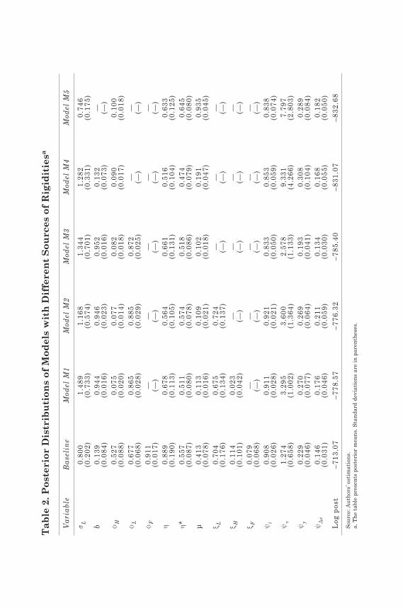
Once the priors have been specified, we estimate the model by first computing the posterior mode and then constructing the posterior distribution with the Metropolis-Hastings algorithm. Table 2 presents the posterior mean of each parameter and its standard deviation under alternative model specifications. In order to compare different models, we also report (in the last row) the value of the log marginal density.

In the baseline case (second column), the inverse of the elasticity of labor supply, σL, has a posterior mean of 0.80, which is slightly smaller than the value reported for the United States by Rabanal and Rubio-Ramírez (2005). The posterior mean of the habit formation coefficient, b, is 0.14. This is consistent with an autoregressive coefficient for consumption, b/(1 + b), of nearly 0.15. This degree of habit formation is below that found for Europe by Adolfson and others (2005b). The posterior mean of the Calvo probability is 0.53 for home goods prices, φH, and 0.68 for wages, φL. This implies that home goods prices are set optimally more frequently than wages: home goods prices are reset every two quarters, on average, whereas wages are kept fixed, on average, for three quarters. Compared with evidence for developed economies, the results for φH imply less sticky prices in the home goods sector, whereas for φL they imply similar values. For example, Adolfson and others (2005b) report values for φH and φL of 0.89 and 0.70, respectively, for the euro area. This is consistent with an average duration of 9.5 quarters for prices and


Ta

ble

2. P

ost

erio

r D

istr

ibu

tio

ns

of

Mo

del

s w

ith

Dif

fere

nt

So

urc

es o

f R

igid

itie

sa

Var

iabl

eB

ase

lin

eM

odel

M1

Mod

el M

2M

odel

M3

Mod

el M

4M

odel

M5

σ L0.

800

1.48

91.

168

1.34

41.

282

0.74

6(0

.202

)(0

.733

)(0

.574

)(0

.701

)(0

.331

)(0

.175

)b

0.13

90.

944

0.94

60.

952

0.13

2—

(0.0

84)

(0.0

16)

(0.0

23)

(0.0

16)

(0.0

73)

(—)

φH

0.52

70.

075

0.07

70.

082

0.09

00.

100

(0.0

88)

(0.0

20)

(0.0

14)

(0.0

18)

(0.0

17)

(0.0

18)

φL

0.67

70.

865

0.88

50.

872

——

(0.0

68)

(0.0

28)

(0.0

29)

(0.0

25)

(—)

(—)

φF

0.91

1—

——

——

(0.0

17)

(—)

(—)

(—)

(—)

(—)

η0.

889

0.67

80.

564

0.66

10.

516

0.63

3(0

.190

)(0

.113

)(0

.105

)(0

.131

)(0

.104

)(0

.125

)η*

0.55

70.

511

0.57

40.

518

0.47

40.

645

(0.0

87)

(0.0

80)

(0.0

78)

(0.0

86)

(0.0

79)

(0.0

80)

μ0.

413

0.11

30.

109

0.10

20.

191

0.93

5(0

.078

)(0

.016

)(0

.021

)(0

.018

)(0

.047

)(0

.045

)ξ L

0.70

40.

675

0.72

4—

——

(0.1

76)

(0.1

34)

(0.1

37)

(—)

(—)

(—)

ξ H0.

114

0.02

3—

——

—(0

.101

)(0

.042

)(—

)(—

)(—

)(—

)ξ F

0.07

9—

——

——

(0.0

68)

(—)

(—)

(—)

(—)

(—)

ψi

0.90

80.

911

0.92

10.

833

0.85

30.

838

(0.0

26)

(0.0

28)

(0.0

21)

(0.0

50)

(0.0

59)

(0.0

74)

ψπ

1.27

43.

295

3.60

02.

578

9.33

17.

797

(0.6

58)

(1.0

02)

(1.3

64)

(1.1

33)

(4.2

66)

(2.8

03)

ψy

0.22

90.

270

0.26

90.

193

0.30

80.

289

(0.0

46)

(0.0

77)

(0.0

64)

(0.0

41)

(0.1

04)

(0.0

84)

ψ∆

e0.

146

0.17

60.

211

0.13

40.

168

0.18

2(0

.031

)(0

.046

)(0

.059

)(0

.030

)(0

.055

)(0

.050

)Lo

g po

st–7

13.0

7–7

78.5

7–7

76.3

2–7

85.4

0–8

31.0

7–8

32.6

8So

urce

: Aut

hors

’ est

imat

ions

.a.

The

tabl

e pr

esen

ts p

oste

rior

mea

ns. S

tand

ard

devi

atio

ns a

re in

par

enth

eses

.



3.5 quarters for wages. In the United States, the average duration of prices and wages is 6.2 and 2.4 quarters, respectively (Rabanal and Rubio-Ramírez, 2005). In a partial equilibrium estimation for Chile, Céspedes, Ochoa, and Soto (2005) find a higher degree of prices stickiness than what we find here, with prices being optimally reset every three to eight quarters. However, they do not estimate the degree of price and wage stickiness simultaneously.

Our estimation of the elasticity of substitution between domestic and foreign goods, η, is 0.89. The estimated value for η* is 0.56. The values for these elasticities are below the estimates for the euro area in Adolfson and others (2005b). At the same time, our results show the existence of both inflation and wage indexation: the coefficients ξL and ξH are estimated to be 0.70 and 0.11, respectively. This latter result implies a reduced-form coefficient on lagged inflation, ξH/(1+βξH), with a value very close to zero. For Chile, Céspedes, Ochoa, and Soto (2005) find a larger value for both ξH and ξH/(1+βξH). We therefore conclude that inflation inertia tends to become less important when we introduce wage indexation. In the next subsection, we test whether ξL and ξH can be removed from the model and the implications that this would have for the remaining coefficients.

Imperfect pass-through from the exchange rate to import prices is a relevant feature of the Chilean economy. The value of, φF, indicates that import prices are kept fixed for around two years, on average. The degree of indexation, ξF , is quantitatively small in this case, at 0.08.

The results for the policy rule coefficients, ψi, ψπ, ψy, and ψ∆e, tend to confirm the findings of previous research. First, we find an important degree of interest rate smoothing: ψi has a posterior mean of nearly 0.9. Second, the response to inflation is relatively more important than the policy response to output and the exchange rate: the posterior mean of ψπ is 1.27 whereas ψy and ψ∆e have a posterior mean of 0.23 and 0.15, respectively.

3.1 Posterior Distribution and Model Comparison

What is the relevance of a particular nominal or real rigidity? Is the monetary policy better described by a forward-looking inflation-targeting Taylor rule or by a rule that reacts to contemporaneous inflation? To answer these questions, we assess the plausibility of alternative models in which we remove some of the rigidities. We also consider models with alternative specifications of the Taylor rule.



We begin by considering a model, M1, that removes the imperfect pass-through and import price inertia. That is, φF = 0, and ξF = 0. As shown in table 2, the log marginal probability density is well below the value under the baseline model. Hence, the fit of the model is clearly worse when we remove imperfect pass-through.

Next, we consider a model, M2, that removes inflation inertia, ξH = 0. The results are shown in the fourth column of table 2. In general, the posterior mean of the coefficients does not change, but this specification has a slightly higher log marginal probability density than M1. Thus, once we remove imperfect pass-through, allowing for ξH = 0 the fit of the model improves. However, the baseline model still delivers a better fit for the Chilean data than M2. In the third alternative specification, we impose no wage indexation, ξL = 0 (see table 2, column 5). This causes the marginal probability density to fall, so we can rule out the hypothesis that ξL = 0. The fourth model we test, M4, additionally removes the assumption that wages are sticky, such that φL = 0. The Bayes factor for this specification is less than one. Allowing for flexible wages thus worsens the model’s ability to fit the aggregate data. Finally, we consider a specification, model M5, in which we also remove the habit coefficient from the Euler equation, b = 0. This model displays a slightly worse fit of the data than model M4. Therefore, although the magnitude of real rigidities is small, empirically it is a relevant feature for explaining the Chilean data.

3.2 Alternative Policy Rules Specifications

Table 3 presents alternative specifications for the policy reaction function. In the baseline case, the Central Bank is reacting to contemporaneous inflation. We test an alternative specification in which the monetary authority is reacting, instead, to expected future inflation (see table 3, column 3). This model fits the data better than the baseline. The Chilean data thus favor a forward-looking behavior by the Chilean Central Bank with respect to inflation. In this case, the values of the nominal and real rigidities do not change significantly, although the policy reaction to expected inflation seems to be higher than in the baseline case. Finally, we test whether a backward-looking specification for the Taylor-type policy rule is preferred and conclude that this model cannot explain the Chilean data better than a model with expected inflation targeting. Forward-looking behavior by the Central Bank is important and consistent with the set of real and nominal rigidities found in the estimation. The presence of real


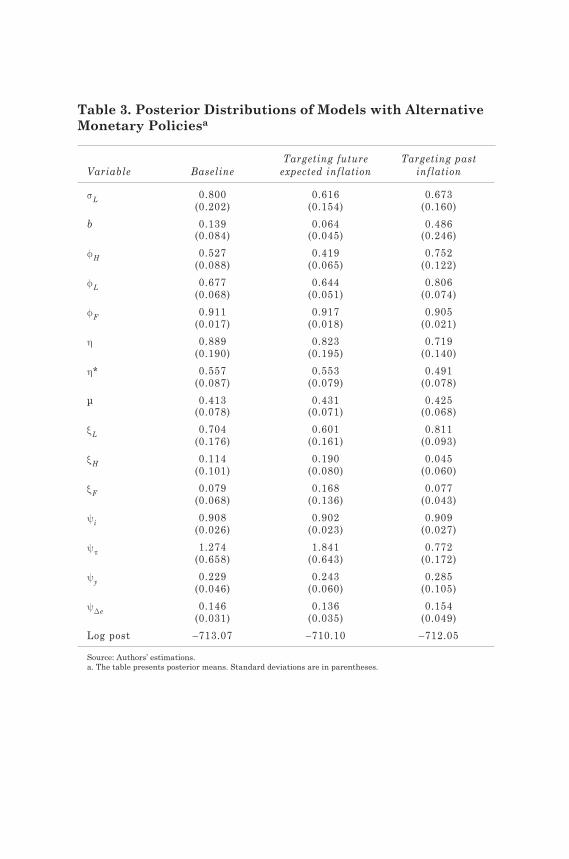
Table 3. Posterior Distributions of Models with Alternative Monetary Policiesa

Variable BaselineTargeting future

expected inflationTargeting past

inflation

σL 0.800 0.616 0.673(0.202) (0.154) (0.160)

b 0.139 0.064 0.486(0.084) (0.045) (0.246)

φH 0.527 0.419 0.752(0.088) (0.065) (0.122)

φL 0.677 0.644 0.806(0.068) (0.051) (0.074)

φF 0.911 0.917 0.905(0.017) (0.018) (0.021)

η 0.889 0.823 0.719(0.190) (0.195) (0.140)

η* 0.557 0.553 0.491(0.087) (0.079) (0.078)

μ 0.413 0.431 0.425(0.078) (0.071) (0.068)

ξL 0.704 0.601 0.811(0.176) (0.161) (0.093)

ξH 0.114 0.190 0.045(0.101) (0.080) (0.060)

ξF 0.079 0.168 0.077(0.068) (0.136) (0.043)

ψ i 0.908 0.902 0.909(0.026) (0.023) (0.027)

ψπ 1.274 1.841 0.772(0.658) (0.643) (0.172)

ψy 0.229 0.243 0.285(0.046) (0.060) (0.105)

ψ∆e 0.146 0.136 0.154(0.031) (0.035) (0.049)

Log post –713.07 –710.10 –712.05

Source: Authors’ estimations.a. The table presents posterior means. Standard deviations are in parentheses.



and nominal rigidities confirms that the effect of monetary policy on inflation occurs with lags. Hence, targeting future expected inflation recognizes that stabilizing current inflation is costly given the presence of real and nominal inertia.

3.3 Subsample Analysis

The inflation-targeting regime in Chile has undergone some changes in the past years. After 1999, Chile embraced a full-fledged inflation-targeting regime with a fixed inflation target and a free-floating exchange rate. To see whether some of the structural coefficients may have changed, we analyze the behavior of the price and wage rigidities in two subsamples: 1990–99 and 2000–05. This exercise is performed for the baseline model. The subsample analysis suggests that both prices and wages were adjusted less frequently after 1999 (see table 4). This result is in line with Céspedes and Soto (in this volume), who find that a credible inflation-targeting regime reduces the incentive to change prices and wages in nominal terms. At the same time, imperfect pass-through from the exchange rate to import prices is a relevant feature of the Chilean economy, with a degree of stickiness that, apparently, does not change over time.

Table 4. Posterior Mode of Price and Wage Rigidities for Subsamples

Variable 1990–99 2000–05

φH 0.400 0.907φL 0.612 0.805φF 0.972 0.913ξL 0.359 0.318ξH 0.137 0.103ξF 0.119 0.070

Source: Authors’ estimations.

We also analyze the subsample behavior of the policy itself, using the baseline specification for the policy reaction function (see table 5). This exercise indicates that the degree of interest rate smoothing increased after 1999. The response to inflation and output also became a little more aggressive after 1999. More importantly, the ratio of ψπ to ψy shrank after 1999 (4.11 versus 2.98). This last result may be an



indication that, in a context of increased policy credibility, the inflation target can be achieved with a relatively less aggressive reaction to inflation vis-à-vis output, reducing the sacrifice ratio. Finally, the policy response to exchange rate movements seems less important in the second subperiod, which is clearly consistent with the elimination of the exchange rate bands.

Table 5. Posterior Mode of Policy Rule Coefficients for Subsamples

Variable 1990–99 2000–05

ψ i 0.682 0.938ψπ 0.649 0.727ψy 0.158 0.244ψ∆e 0.321 0.159

Source: Authors’ estimations.

4. CONCLUSIONS

In this paper, we have derived a microfounded model that features habit formation in the utility function and considers both sticky prices and wages. We also introduced indexation in prices and wages, and we incorporated imperfect pass-through from the exchange rate to import prices.

These nominal and real rigidities may be features that characterize a small open economy like Chile. The main question this paper addresses, then, is the extent to which nominal and real rigidities are important in explaining the behavior of the aggregate data in Chile during the inflation-targeting period. This question is particularly important from a policymaker’s perspective. Identifying the level of nominal and real rigidities that are present in the economy is a relevant step toward the efficient design of monetary policy. The existence (or absence) of certain rigidities may have very different implications for the trade-off between output and inflation stabilization that central banks face.

We address this question in the context of a structural model that is estimated using Bayesian techniques. The advantage of this approach is that it is system-based and enables us to incorporate additional information, not contained in the actual data, into the parameter estimation. Moreover, this approach can cope with identification and misspecification problems. In this context, we also investigate how



the Chilean Central Bank has designed its policy in the inflation-targeting period. To do this, we introduce a Taylor-type policy rule in the microfounded model and assess whether this rule has reacted to expected, contemporaneous, or lagged inflation.

Our main results are as follows. First, models with both price and wage rigidities best account for the Chilean data. Notably, the degree of wage rigidities is higher than that of domestic prices. Our results show that nominal wages are adjusted optimally every three quarters, on average. In contrast, prices are re-optimized every two quarters. The subsample analysis suggests that both prices and wages were adjusted less frequently after 1999 than before. This result could reflect the increased credibility of the inflation-targeting regime, which would give price and wage setters less of an incentive to adjust nominal prices and wages. At the same time, imperfect pass-through from the exchange rate to import prices is a relevant feature of the Chilean economy.

Second, adding wage indexation clearly improves the fit of the model. This level of indexation is comparatively larger than that of domestic and import prices. Wage indexation generates a more persistent response of inflation to shocks, and it is one of the determinants of the policy trade-off.

Third, real rigidities such as habit formation also provide a better account of the aggregate data, although the possible values of it are quantitatively small.

Fourth, models with a Taylor rule that reacts to expected inflation characterize monetary policy in the sample period better than models with a Taylor rule that reacts to contemporaneous inflation. As found in previous studies, the policy response to inflation is comparatively larger than the response to output and the exchange rate. Moreover, the subsample analysis indicates that the degree of interest rate smoothness increased after 1999. The response to inflation relative to output also became less aggressive after 1999. In a context of increased policy credibility, the inflation target can be achieved with a smaller trade-off between inflation and output fluctuations, reducing the sacrifice ratio.

Overall, our results confirm the relevance of a wide set of frictions for explaining the behavior of the Chilean economy. These frictions are the key elements that determine the optimality of alternative ways of designing monetary policy. Hence, the results presented here raise two questions: to what extent has the Chilean Central Bank reacted to both price and wage inflation, and what is the optimal response to this type of friction? We leave these questions to future research.



APPENDIX The Steady State of the Model

We assume that the long-run income per capita growth rate is gy, and the steady-state inflation rate is πC. These assumption imply a nominal interest rate given by i = (1 + gy)(1 + πC)/β – 1. The foreign interest rate and inflation rate are i* and π*. The arbitrage condition in the steady state implies an external premium equal to

Θ =+

+++

11

11

iiCππ*

*.

In the long-run steady state, the ratio of net exports to GDP is denoted by NX/Y. The share of imported goods in total consumption is α, and the share of domestically produced (H) goods in total GDP is denoted by YH/Y. We use these statistics to find

CY

NXY

= −1 ;

MY

CY

CC

CY

NXY

F F= = = −

α 1 ;

XY

NXY

MY

NXY

= + = −( )+1 α α ;

CY

CC

CY

NXY

H H= = −( ) −

1 1α ;

CY

CC

CY

NXY

F F= = −

α 1 ; and

CY

Y CY

YY

NXY

H H H H*

=−

= − −( ) −

1 1α .

Finally, using the foreign interest rate and the ratio of net exports to GDP, we derive an expression for the ratio of net foreign assets to GDP:

eBY

NXY i gy

** *

=+( )

−+( ) +( )

11

11 1Θ π

.



REFERENCES

Adão, B., I. Correia, and P. Teles. 2003. “Gaps and Triangles.” Review of Economic Studies 70(4): 699–713.

Adolfson, M., S. Laseén, J. Lindé, and M. Villani. 2005a. “An Estimated New Keynesian Model for a Small Open Economy.” Stockholm: Sveriges Riksbank, mimeo.

. 2005b. “Bayesian Estimation of an Open Economy DSGE Model with Incomplete Pass-Through.” Working paper 179. Stockholm: Sveriges Riksbank.

Altig, D., L. Christiano, M., Eichenbaum, and J. Lindé. 2004. “Firm-Specific Capital, Nominal Rigidities and the Business Cycle.” Working Paper No. 176, Sveriges Riksbank.

Benigno, G. and P. Benigno. 2003. “Price Stability in Open Economies.” Review of Economic Studies 70(4): 743–64.

Benigno, P. and M. Woodford. 2004. “Optimal Stabilization Policy When Wages and Prices are Sticky: The Case of a Distorted Steady State”. NBER Working Paper N°10839.

Bergoeing, R. and R. Soto. 2005. “Testing Real Business Cycle Models in an Emerging Economy.” In General Equilibrium Models for the Chilean Economy, edited by R. Chumacero and K. Schmidt-Hebbel, 221–60. Santiago: Central Bank of Chile.

Blanchard, O. and J. Galí. 2005. “Real Wage Rigidities and the New Keynesian Model.” Working paper 05-28. Massachusetts Institute of Technology, Department of Economics.

Brubakk, L., T.A. Husebø, S. McCaw, D. Muir, and others. 2005. “Finding NEMO: From the Global Economy Model (GEM) to a National Core Model.” Oslo: Norges Bank.

Caballero, R. and A. Krishnamurthy. 2001. “International and Domestic Collateral Constraints in a Model of Emerging Market Crises.” Journal of Monetary Economics 48(3): 513–48.

Calvo, G. 1983. “Staggered Prices in a Utility-Maximizing Framework.” Journal of Monetary Economics 12(3): 383–98.

Caputo, R. 2005. “Exchange Rates, Inflation, and Monetary Policy Objectives in Open Economies: The Experience of Chile.” In Exchange Rates, Capital Flows, and Policy, edited by R. Driver, P. Sinclair, and C. Thoenissen, 39–57. Routledge.

Caputo, R. and F. Liendo. 2005. “Monetary Policy, Exchange Rate, and Inflation Inertia in Chile: A Structural Approach.” Working paper 352. Santiago: Central Bank of Chile.



Céspedes, L.F., M. Ochoa, and C. Soto. 2005. “An Estimated New Keynesian Phillips Curve for Chile.” Santiago: Central Bank of Chile.

Chari, V. V., P. Kehoe, and E. McGrattan. 2000. “Sticky Price Models of the Business Cycle: Can the Contract Multiplier Solve the Persistence Problem?” Econometrica 68(5): 1151–81.

Christiano, L., M. Eichenbaum, and C. Evans. 2005. “Nominal Rigidities and the Dynamic Effects of a Shock to Monetary Policy.” Journal of Political Economy 113(1): 1–45.

Clarida, R., J. Galí, and M. Gertler. 1999. “The Science of Monetary Policy: A New Keynesian Perspective.” Journal of Economic Literature 37(4): 1661–707.

Corbo, V. 2002. “Monetary Policy in Latin America in the 1990s.” In Monetary Policy: Rules and Transmission Mechanisms, edited by N. Loayza, and R. Soto, 117–66. Santiago: Central Bank of Chile.

Corbo, V. and J. Tessada. 2005. “Response to External and Inflation Shocks in a Small Open Economy.” In General Equilibrium Models for the Chilean Economy, edited by R. Chumacero and K. Schmidt-Hebbel, 29–56. Santiago: Central Bank of Chile.

Duncan, R. 2005. “How Well Does a Monetary Dynamic Equilibrium Model Account for Chilean Data?” In General Equilibrium Models for the Chilean Economy, edited by R. Chumacero and K. Schmidt-Hebbel, 189–220. Santiago: Central Bank of Chile.

Erceg, C., D W. Henderson, and A. T. Levin. 2000. “Optimal Monetary Policy with Staggered Wage and Price Contracts.” Journal of Monetary Economics 46(2): 281–313.

Fernández-Villaverde, J. and J. Rubio-Ramírez. 2004. “Comparing Dynamic Equilibrium Economies to Data: A Bayesian Approach.” Journal of Econometrics 123(1): 153–87.

Fuhrer, J.C. 2000. “Habit Formation in Consumption and Its Implications for Monetary Policy Models.” American Economic Review 90(3): 367–90.

Galí, J. and T. Monacelli. 2005. “Monetary Policy and Exchange Rate Volatility in a Small Open Economy.” Review of Economic Studies 72(3): 707–34.

Gallego, F., K. Schmidt-Hebbel, and L. Servén. 2005. “General Equilibrium Dynamics of Foreign Shocks and Policy Changes in Chile.” In General Equilibrium Models for the Chilean Economy, edited by R. Chumacero and K. Schmidt-Hebbel, 113–62. Santiago: Central Bank of Chile.

García, C., P. García, I. Magendzo, and J.E. Restrepo. 2005. “The Monetary Transmission Mechanism in Chile: A Medium-Sized



Macroeconometric Model.” In General Equilibrium Models for the Chilean Economy, edited by R. Chumacero and K. Schmidt-Hebbel, 57–112. Santiago: Central Bank of Chile.

García, P., L.Ó. Herrera, and R. Valdés. 2002. “New Frontiers for Monetary Policy in Chile.” In General Equilibrium Models for the Chilean Economy, edited by N. Loayza and R. Soto, 627–49. Santiago: Central Bank of Chile.

Geweke, J. 1998. “Using Simulation Methods for Bayesian Econometric Models: Inference, Development, and Communication.” Staff report 249. Federal Reserve Bank of Minneapolis.

Goodfriend, M., and R. King. 1997. “The New Neoclassical Synthesis and the Role of Monetary Policy.” In NBER Macroeconomics Annual 1997, edited by B.S. Bernanke and J. Rotemberg, 231–83. MIT Press.

Jacquinot, P., R. Mestre, and M. Spitzer. 2005. “An Open-Economy DSGE Model of the Euro Area.” Frankfurt: European Central Bank.

Jadresic, E. 2002. “The Macroeconomic Consequences of Wage Indexation Revisited.” In Indexation, Inflation, and Monetary Policy, edited by F. Lefort and K. Schmidt-Hebbel, 207–57. Santiago: Central Bank of Chile.

Lama, R. and J. P. Medina. 2004. “Optimal Monetary Policy in a Small Open Economy with Sticky Prices and Segmented Asset Markets.” Working paper 286. Santiago: Central Bank of Chile.

Leeper, E. and T. Zha. 2000. “Assessing Simple Policy Rules: A View from a Complete Macro Model.” Working paper 2000-19. Federal Reserve Bank of Atlanta.

Lubik, T. and F. Schorfheide (2006). “Do Central Banks Respond to Exchange Rate Movements? A Structural Investigation.” forthcoming, Journal of Monetary Economics.

Medina, J.P. and C. Soto. 2005. “Model for Analysis and Simulations (MAS): A New DSGE for the Chilean Economy.” Santiago: Central Bank of Chile.

Medina, J.P. and R. Valdés. 2002. “Optimal Monetary Policy Rules When the Current Account Matters.” In Monetary Policy: Rules and Transmission Mechanisms, edited by N. Loayza and K. Schmidt-Hebbel, 65–94. Santiago: Central Bank of Chile.

Parrado, E. and A. Velasco. 2002. “Alternative Monetary Rules in the Open Economy: A Welfare-Based Approach.” In Inflation Targeting: Design, Performance, Challenges, edited by N. Loayza and R. Soto: 295–348. Santiago: Central Bank of Chile.



Rabanal, P. and J. Rubio-Ramírez. 2005. “Comparing New Keynesian Models of the Business Cycle: A Bayesian Approach.” Journal of Monetary Economics 52(6): 1151–66.

Rotemberg, J. and M. Woodford. 1997. “An Optimization-Based Econometric Framework for the Evaluation of Monetary Policy.” In NBER Macroeconomics Annual 1997, edited by B. S. Bernanke and J. Rotemberg, 231–83, 297–46. MIT Press.

Schmidt-Hebbel, K. and M. Tapia. 2002. “Inflation Targeting in Chile.” North American Journal of Economics and Finance 13: 125–46.

Schmitt-Grohé, S. and M. Uribe. 2001. “Stabilization Policy and the Costs of Dollarization.” Journal of Money, Credit, and Banking 33: 482-509

. 2003. “Closing Small Open Economy Models.” Journal of International Economics 61(1): 163–85.

. 2004. “Optimal Fiscal and Monetary Policy under Sticky Prices.” Journal of Economic Theory 114(2): 198–230.

. 2005. “Optimal Fiscal and Monetary Policy in a Medium-Scale Macroeconomic Model: Expanded Version.” Working paper 11417. Cambridge, Mass.: National Bureau of Economic Research.

Sims, C.A. 2002. “Solving Linear Rational Expectation Models.” Computational Economics 20: 1–20.

Smets, F., and R. Wouters. 2003a. “An Estimated Stochastic Dynamic General Equlibrium Model of the Euro Area.” Journal of the European Economic Association 1(5): 1123–75.

. 2003b. “Shocks and Frictions in U.S. Business Cycles: A Bayesian DSGE Approach.” Frankfurt: European Central Bank.

Uhlig, H. 1997. “A Toolkit for Analyzing Nonlinear Dynamic Stochastic Models Easily,” University of Tilburg.

Woodford, M. 2001. “Inflation Stabilization and Welfare.” Working paper 8071. Cambridge, Mass.: National Bureau of Economic Research.


Documents

NEW K M C I -T PERIOD Rodrigo Caputo · discussants, Renzo Rossini and Raphael Bergoeing, and Sebastián Edwards, Douglas Laxton, Andrew Levin, David Rappoport, Claudio Soto, and