Embed Size (px)
Citation preview

NEW JERSEY TRAFFIC ANDREVENUE STUDY
Garden State Parkway Asset Appraisal
Final Report
January 2008
Prepared for: Prepared by:
State of New JerseyDepartment of TreasuryState House125 West State StreetTrenton, NJ 08625
Steer Davies Gleave in association with CRAInternational and EDR Group
28-32 Upper GroundLondonSE1 9PD
+44 (0)20 7919 8500www.steerdaviesgleave.com

Garden State Parkway Asset Appraisal
Contents
Contents Page
1. INTRODUCTION 1
Statement of Objectives 1
Approach and Analysis Undertaken 1
Report Contents 2
2. THE GARDEN STATE PARKWAY 3
Project Overview 3
Tolling Regime 9
2006 Transactions and Revenue Levels 10
Behavioral Research 26
Summary 29
3. THE FORECASTING METHODOLOGY 31
Introduction 31
Impact of Toll Changes and Congestion 33
Existing and Future Capacity Constraints 34
4. TRAFFIC GROWTH 35
Introduction 35
Economic Development 35
Trip Rates 37
Vollmer Forecasts 43
Steer Davies Gleave Forecasts 44
5. FORECASTS 52
Introduction 52
Toll Scenarios 54
GSP Traffic and Revenue Forecasts 56
Review of Responses in Demand to Toll Changes 62
APPENDICES
A: MAPS
B: FORECASTS
C: LANE EXPANSIONS
Garden State Parkway Asset Appraisal
Glossary
GLOSSARY OF DEFINED TERMS:
• Annual Average Weekday Traffic (AADTw)
• Atlantic City Expressway (ACE)
• Annual Average Daily Traffic (AADT)
• CRA International (CRAI)
• EDR Group (EDRG)
• Electronic Toll Collection (ETC)
• Federal Highway Administration (FHWA)
• Garden State Parkway (GSP)
• Gross Domestic Product (GDP)
• Gross Regional Product (GRP)
• Level of Service (LOS)
• New Jersey Department of Transportation (NJDOT)
• New Jersey Highway Authority (NJHA)
• North Jersey Regional Model (NJTPA)
• New Jersey Turnpike (NJTP)
• New Jersey Turnpike Authority (NJTA)
• Origin-Destination (O-D)
• Rutgers State University of New Jersey’s Economic Advisory Service (RECON)
• South Jersey Regional Model (SJTPO)
• South Jersey Transportation Authority (SJTA)
• U.S. Highway Capacity Manual (HCM)
• Vehicle Miles Traveled (VMT)
• Wilbur Smith and Associates (WSA)

Garden State Parkway Asset Appraisal
Disclaimer
DISCLAIMER
This report has been prepared for the State of New Jersey as an initial overview of issues relevant totraffic and revenue projections to assist in the preparation of the possibility of monetizing a numberof the transport assets at present owned and operated by the State (or its agents). This report isintended to provide an overview of relevant issues and does not provide investment grade analysis.
The analysis and projections of traffic and revenue contained within this document represent thebest estimates of Steer Davies Gleave at this stage. While the forecasts are not precise forecasts,they do represent, in our view, a reasonable expectation for the future, based on the informationavailable as of the date of this report.
However, the estimates contained within this document rely on numerous assumptions andjudgments and are influenced by external circumstances that are subject to changes that maymaterially affect the conclusions drawn.
In addition, the view and projections contained within this report rely on data collected by thirdparties. Steer Davies Gleave has conducted independent checks of this data where possible, but doesnot guarantee the accuracy of this data.
No parties other than the State of New Jersey can place reliance on it.
Garden State Parkway Asset Appraisal
1
1. INTRODUCTION
Statement of Objectives
1.1 The State of New Jersey is considering the possibility of monetizing a number of thetransport assets at present owned and operated by the State or certain authorities in, butnot of, the State. These include the New Jersey Turnpike (NJTP), the Atlantic CityExpressway (ACE), the Garden State Parkway (GSP) and Route 440 (between the NJTPand the Outer Bridge Crossing).
1.2 The State has appointed a financial advisor to help it understand how such a process mightbe carried out – and it has appointed Steer Davies Gleave, together with CRAInternational (CRAI) and the EDR Group (EDRG), as traffic and revenue advisors. Ourbrief is to provide assistance in the estimation of the traffic that might be carried on theassets, and the toll revenue that might be generated.
1.3 Our overall work for this assignment consisted of two phases:
• Phase 1: Scoping; and
• Phase 2: Asset by Asset Appraisal of Future Traffic and Revenue streams.
1.4 The objective of the Phase 1 work was to prepare an initial review of the likely levels oftraffic and revenue on the target roads across the likely duration of the forecast period.This work comprised the collection and collation of existing traffic data for each road, aninitial review of the key drivers of future traffic growth and a literature review of elasticityparameters (a key determinant of traffic responsiveness to changes in tolls).
1.5 In Phase 2 work we have built on the analysis carried out for Phase 1 and developed amodeling framework that can explore the base assignment to the target facility under arange of scenarios – and for different traffic types. It has been built to allow sensitivitytesting of a range of factors including values of time – and allows for rapid testing ofdifferent tolling scenarios. We have adopted a number of existing modeling tools to act asfocused network models and have developed separate spreadsheet based revenue modelsto focus on the important traffic categories and the choices that road users would face.
Approach and Analysis Undertaken
1.6 In conjunction with our partners at CRAI and EDRG, we have undertaken the followingkey tasks as part of both work phases:
• Developed an overview of traffic and revenue on the road assets to understand thecomposition of traffic volumes by time of day and location;
• Reviewed the key economic issues and the likely impact on traffic of estimatedgrowth in key economic parameters;
• Developed a modeling framework to explore the base assignment to the target facilityunder a range of scenarios – and for different traffic types;
Garden State Parkway Asset Appraisal
2
• Undertaken a number of travel time surveys to assist in the model validation process,in particular to check that modeled travel times are representative of observedjourney times;
• Undertaken an internet based attitudinal surveys with New Jersey residents to supportour forecasting assumptions; and
• Reviewed relevant North American ‘price elasticity of demand’ studies to assess thelikely impact of toll changes on traffic volumes.
1.7 In carrying out this work we reviewed and relied on third party reports and data withoutindependent verification. However, in most instances we used recent data collected byrecognized experts or firms with nationally recognized credentials.
Report Contents
1.8 The purpose of this document is to present our traffic and revenue forecasts for the GSPand to provide an overview of the key assumptions made as part of the process to developthese forecasts. A separate report describes the background to our work and methodologyin more detail.
1.9 This document is structured as follows:
• Chapter 2 provides an overview of the GSP and presents 2006 traffic and revenues;
• Chapter 3 presents an overview of our forecasting methodology, discusses keyforecasting issues and summarizes key forecasting assumptions;
• Chapter 4 discusses how future traffic growth rates have been derived and defined;and
• Chapter 5 presents traffic and revenue forecasts for the facilities.
Garden State Parkway Asset Appraisal
3
2. THE GARDEN STATE PARKWAY
Project Overview
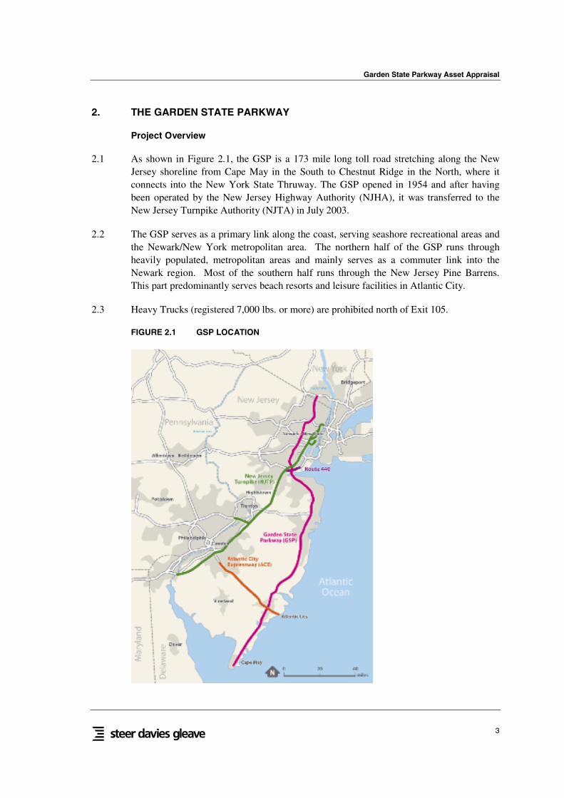
2.1 As shown in Figure 2.1, the GSP is a 173 mile long toll road stretching along the NewJersey shoreline from Cape May in the South to Chestnut Ridge in the North, where itconnects into the New York State Thruway. The GSP opened in 1954 and after havingbeen operated by the New Jersey Highway Authority (NJHA), it was transferred to theNew Jersey Turnpike Authority (NJTA) in July 2003.
2.2 The GSP serves as a primary link along the coast, serving seashore recreational areas andthe Newark/New York metropolitan area. The northern half of the GSP runs throughheavily populated, metropolitan areas and mainly serves as a commuter link into theNewark region. Most of the southern half runs through the New Jersey Pine Barrens.This part predominantly serves beach resorts and leisure facilities in Atlantic City.
2.3 Heavy Trucks (registered 7,000 lbs. or more) are prohibited north of Exit 105.
FIGURE 2.1 GSP LOCATION
Garden State Parkway Asset Appraisal
4
2.4 The GSP interacts with most major highway routes throughout New Jersey, including:
• ACE (Exit 38 and 38A)
• I-195, providing access to Belmar and Trenton (Exit 98)
• US 9/NJ 440, providing access to Woodbridge and Staten Island (Exit 127)
• New Jersey Turnpike (Exit 129)
• I-78/NJTP, providing access to Newark Airport and the west, (Exit 142)
• I-280, providing access to Newark and the west (Exit 145)
• I-80, providing access to George Washington Bridge and the west (Exit 159)
2.5 The GSP is both a commuter road and a link to leisure facilities.
2.6 The northern end of the road is a functional commuter highway, serving users into theNew York area and running through densely populated urban and suburban areas.
2.7 South of the Raritan River, the GSP serves more rural regions, following the shorelinewith its beach resorts and casinos, from Monmouth to Cape May counties.
2.8 Because trucks are not permitted along its entire length, commercial through traffic is notsignificant.
Road Configuration
2.9 The GSP is a grade-separated limited access roadway with a speed limit of 65 mph frommilepost 27 north to milepost 123, and from milepost 163 north to the New Jersey-NewYork border. Elsewhere, the maximum posted speed limit is 55 mph (with the exceptionof the Driscoll Bridge, where the posted speed limit is 45 mph).
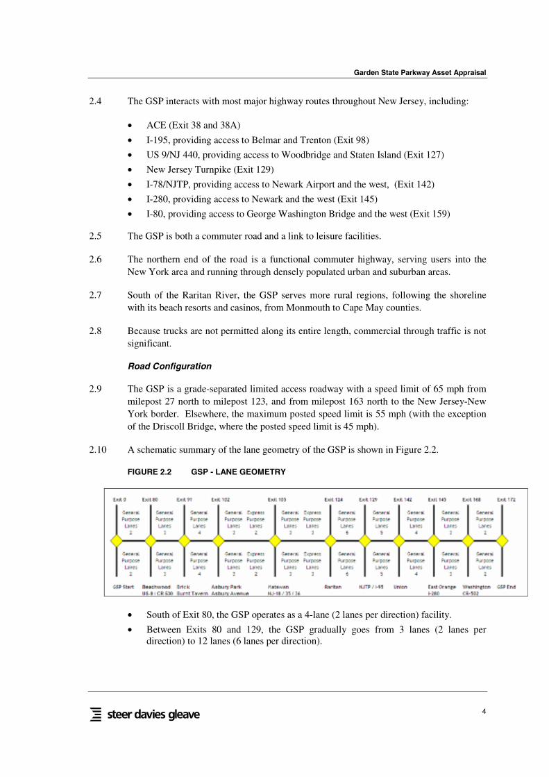
2.10 A schematic summary of the lane geometry of the GSP is shown in Figure 2.2.
FIGURE 2.2 GSP - LANE GEOMETRY
• South of Exit 80, the GSP operates as a 4-lane (2 lanes per direction) facility.
• Between Exits 80 and 129, the GSP gradually goes from 3 lanes (2 lanes perdirection) to 12 lanes (6 lanes per direction).

Garden State Parkway Asset Appraisal
5
• Between the Asbury Park and Raritan toll barriers, the GSP splits into express andlocal lanes (in this section there are 10 to 12 lanes). The express lanes have access tono exits, except for Exit 105 and Exit 117.
• Between Exits 129 and 172, the number of lanes on the GSP gradually decreasesfrom 10 (5 lanes per direction) to 4 (2 lanes per direction) until the northern extremityof the road.
Competing Routes
2.11 A number of competing routes exist along the length of the GSP. In the North (Exit 172to Exit 127) it competes with the I-287 and NJTP.
2.12 At the southern end, the I-287 connects into the GSP as Route 440 at Exit 10 of the NJTPand extends westwards to Pluckemin, from where it extends northwards, parallel to theGSP, while bypassing the New York/Northern New Jersey Metropolitan areas. At itsnorthern end, it connects with the New York State Thruway. The route offers an un-tolledalternative to the GSP for journeys to and from the New York/Northern New JerseyMetropolitan area and upstate New York or further north along the eastern seaboard.
2.13 The NJTP offers an alternative for through journeys from New York State to central NewJersey. It also offers users an alternative for all or at least the southern portion of tripsfrom central New Jersey to more northerly areas such as Newark. Users may choose theNJTP as it may provide a quicker journey although, albeit at a higher price for some tripsin the Central to Northern sections.
2.14 The I-287 and NJTP are shown in Figure 2.3 below.
FIGURE 2.3 GSP - COMPETING ROUTES: NORTHERN SECTION
Garden State Parkway Asset Appraisal
6
Southern and Central Sections (Exit 125 to Exit 0)
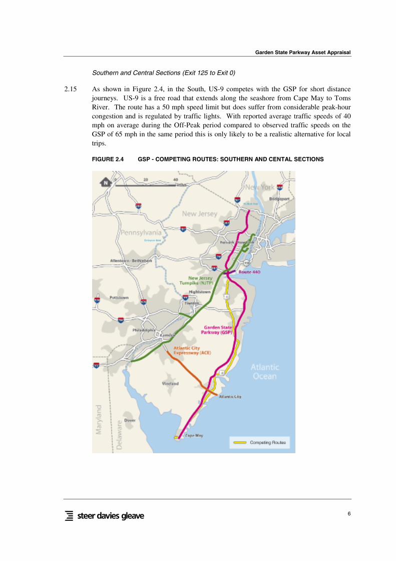
2.15 As shown in Figure 2.4, in the South, US-9 competes with the GSP for short distancejourneys. US-9 is a free road that extends along the seashore from Cape May to TomsRiver. The route has a 50 mph speed limit but does suffer from considerable peak-hourcongestion and is regulated by traffic lights. With reported average traffic speeds of 40mph on average during the Off-Peak period compared to observed traffic speeds on theGSP of 65 mph in the same period this is only likely to be a realistic alternative for localtrips.
FIGURE 2.4 GSP - COMPETING ROUTES: SOUTHERN AND CENTAL SECTIONS
Garden State Parkway Asset Appraisal
7
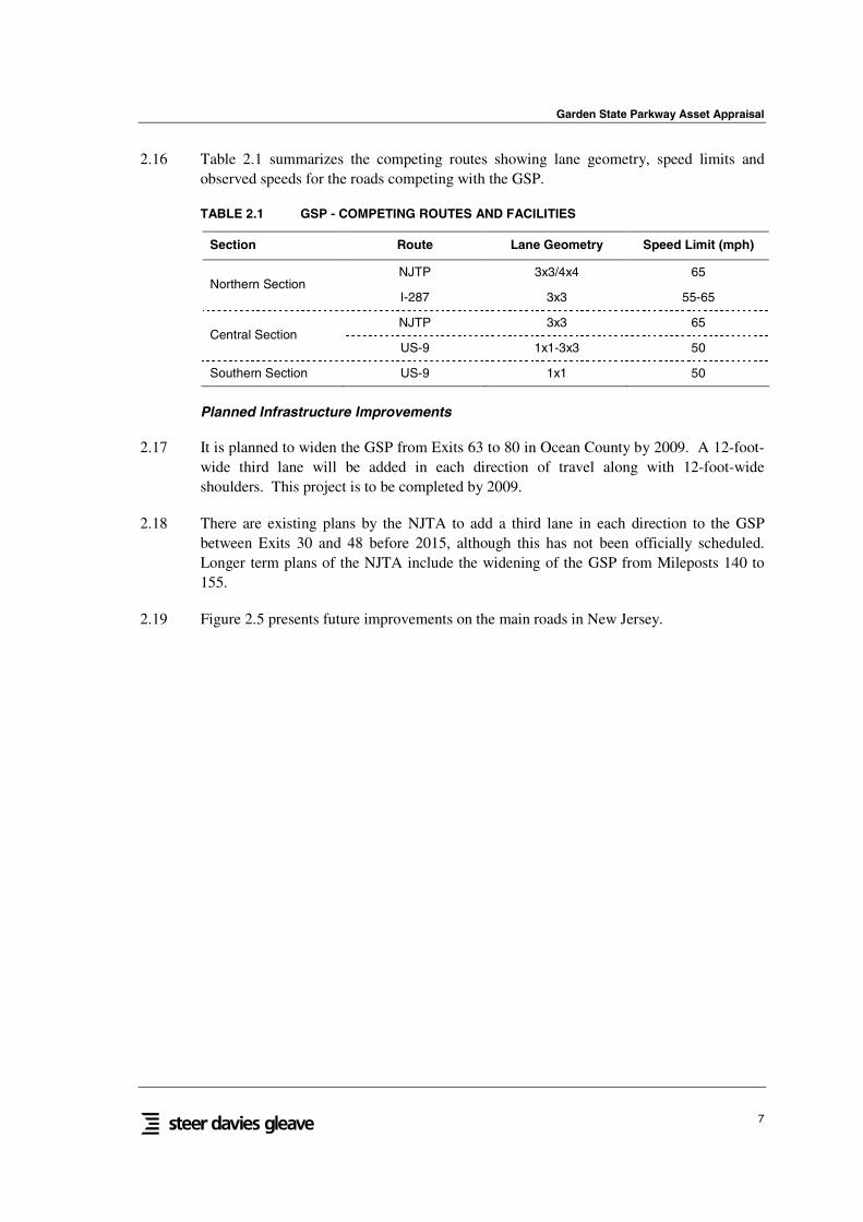
2.16 Table 2.1 summarizes the competing routes showing lane geometry, speed limits andobserved speeds for the roads competing with the GSP.
TABLE 2.1 GSP - COMPETING ROUTES AND FACILITIES
Section Route Lane Geometry Speed Limit (mph)
NJTP 3x3/4x4 65 Northern Section
I-287 3x3 55-65
NJTP 3x3 65 Central Section
US-9 1x1-3x3 50
Southern Section US-9 1x1 50
Planned Infrastructure Improvements
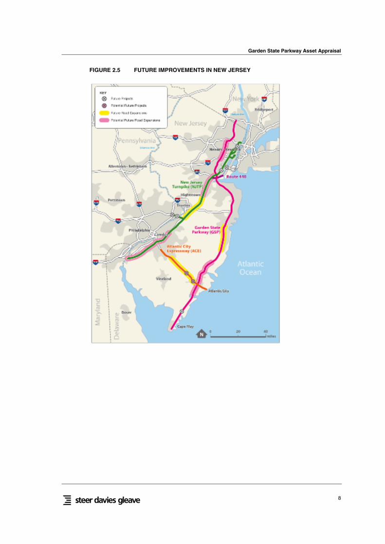
2.17 It is planned to widen the GSP from Exits 63 to 80 in Ocean County by 2009. A 12-foot-wide third lane will be added in each direction of travel along with 12-foot-wideshoulders. This project is to be completed by 2009.
2.18 There are existing plans by the NJTA to add a third lane in each direction to the GSPbetween Exits 30 and 48 before 2015, although this has not been officially scheduled.Longer term plans of the NJTA include the widening of the GSP from Mileposts 140 to155.
2.19 Figure 2.5 presents future improvements on the main roads in New Jersey.
Garden State Parkway Asset Appraisal
8
FIGURE 2.5 FUTURE IMPROVEMENTS IN NEW JERSEY

Garden State Parkway Asset Appraisal
9
Tolling Regime
2.20 The GSP operates as an ‘open system’ whereby users pay tolls at regular intervals alongthe length of the road and at certain exits. On some short distance sections, vehicles canuse the road without paying tolls. Maps showing the location of toll barriers and rampsare included in Appendix A.
2.21 Historically, tolls were collected in both directions at all barriers. In order to reduce thecongestion associated with toll collection, an initiative was undertaken to convert eighttoll barriers to one-way toll collection. At these toll plazas, a single 70-cent toll is nowcollected in only one direction with the other direction free, whereas previously a 35-centtoll was collected in each direction.
2.22 For consecutive one-way barriers, tolls are collected in alternating directions to limit theincentive for selecting alternative routes. The following toll plazas were made one-way:Cape May, Great Egg, New Gretna, Asbury Park, Raritan, Union, Essex, and Bergen. InMarch 2007, Barnegat was converted to one-way. As of March 2007, the remaining two-way barriers (Hillsdale/Pascack Valley and Toms River) are not scheduled to be convertedto one-way tolling.
2.23 Tolls are charged differentially according to vehicle size with the toll classifications basedon the number of axles, with passenger cars, 2-axle, 3-axle, 4-axle, 5-axle and 6-axletrucks making up Classes 1-6 respectively.
TABLE 2.2 GSP - 2006 TOLLS FOR SELECTED KEY MOVEMENTS (CLASS 1, CASHPAYMENT)
Exit 0 Exit 38 Exit 129 Exit 142 Exit 172
Exit 0 (South Termini) $0.70 $2.80 $2.80 $4.55
Exit 38 (Atlantic City) $0.70 $2.10 $2.10 $3.85
Exit 129 (NJTP) $2.10 $1.40 $0.00 $1.75
Exit 142 (NJTP) $2.10 $1.40 $0.00 $1.75
Exit 172 (North Termini) $3.15 $2.45 $1.05 $1.05
Source: NJTA
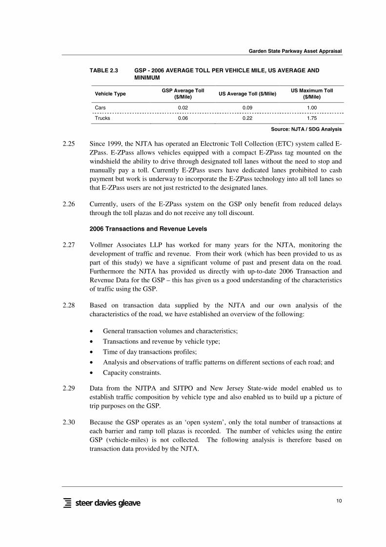
2.24 As mentioned, heavy vehicles are charged more, according to the number of axles pervehicle, with toll rates varying by a factor of 2.6. With a cost-per-mile rate ofapproximately $0.02 per mile, the GSP is currently the least costly toll road in the UnitedStates.
Garden State Parkway Asset Appraisal
10
TABLE 2.3 GSP - 2006 AVERAGE TOLL PER VEHICLE MILE, US AVERAGE ANDMINIMUM
Vehicle TypeGSP Average Toll
($/Mile)US Average Toll ($/Mile)
US Maximum Toll($/Mile)
Cars 0.02 0.09 1.00
Trucks 0.06 0.22 1.75
Source: NJTA / SDG Analysis
2.25 Since 1999, the NJTA has operated an Electronic Toll Collection (ETC) system called E-ZPass. E-ZPass allows vehicles equipped with a compact E-ZPass tag mounted on thewindshield the ability to drive through designated toll lanes without the need to stop andmanually pay a toll. Currently E-ZPass users have dedicated lanes prohibited to cashpayment but work is underway to incorporate the E-ZPass technology into all toll lanes sothat E-ZPass users are not just restricted to the designated lanes.
2.26 Currently, users of the E-ZPass system on the GSP only benefit from reduced delaysthrough the toll plazas and do not receive any toll discount.
2006 Transactions and Revenue Levels
2.27 Vollmer Associates LLP has worked for many years for the NJTA, monitoring thedevelopment of traffic and revenue. From their work (which has been provided to us aspart of this study) we have a significant volume of past and present data on the road.Furthermore the NJTA has provided us directly with up-to-date 2006 Transaction andRevenue Data for the GSP – this has given us a good understanding of the characteristicsof traffic using the GSP.
2.28 Based on transaction data supplied by the NJTA and our own analysis of thecharacteristics of the road, we have established an overview of the following:
• General transaction volumes and characteristics;
• Transactions and revenue by vehicle type;
• Time of day transactions profiles;
• Analysis and observations of traffic patterns on different sections of each road; and
• Capacity constraints.
2.29 Data from the NJTPA and SJTPO and New Jersey State-wide model enabled us toestablish traffic composition by vehicle type and also enabled us to build up a picture oftrip purposes on the GSP.
2.30 Because the GSP operates as an ‘open system’, only the total number of transactions ateach barrier and ramp toll plazas is recorded. The number of vehicles using the entireGSP (vehicle-miles) is not collected. The following analysis is therefore based ontransaction data provided by the NJTA.
Garden State Parkway Asset Appraisal
11
2006 Toll Transactions
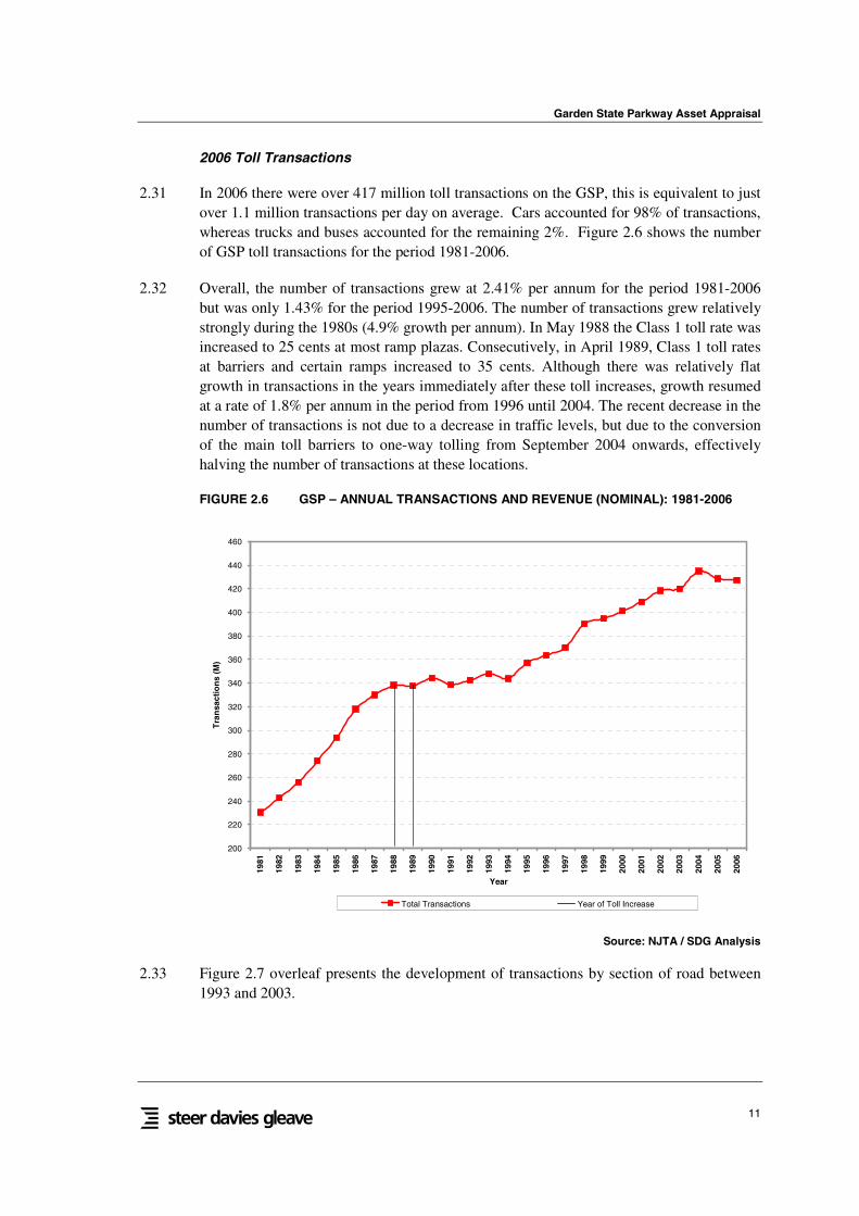
2.31 In 2006 there were over 417 million toll transactions on the GSP, this is equivalent to justover 1.1 million transactions per day on average. Cars accounted for 98% of transactions,whereas trucks and buses accounted for the remaining 2%. Figure 2.6 shows the numberof GSP toll transactions for the period 1981-2006.
2.32 Overall, the number of transactions grew at 2.41% per annum for the period 1981-2006but was only 1.43% for the period 1995-2006. The number of transactions grew relativelystrongly during the 1980s (4.9% growth per annum). In May 1988 the Class 1 toll rate wasincreased to 25 cents at most ramp plazas. Consecutively, in April 1989, Class 1 toll ratesat barriers and certain ramps increased to 35 cents. Although there was relatively flatgrowth in transactions in the years immediately after these toll increases, growth resumedat a rate of 1.8% per annum in the period from 1996 until 2004. The recent decrease in thenumber of transactions is not due to a decrease in traffic levels, but due to the conversionof the main toll barriers to one-way tolling from September 2004 onwards, effectivelyhalving the number of transactions at these locations.
FIGURE 2.6 GSP – ANNUAL TRANSACTIONS AND REVENUE (NOMINAL): 1981-2006
200
220
240
260
280
300
320
340
360
380
400
420
440
460
1981
1982
1983
1984
1985
1986
1987
1988
1989
1990
1991
1992
1993
1994
1995
1996
1997
1998
1999
2000
2001
2002
2003
2004
2005
2006
Year
Tra
nsa
ctio
ns
(M)
Total Transactions Year of Toll Increase
Source: NJTA / SDG Analysis
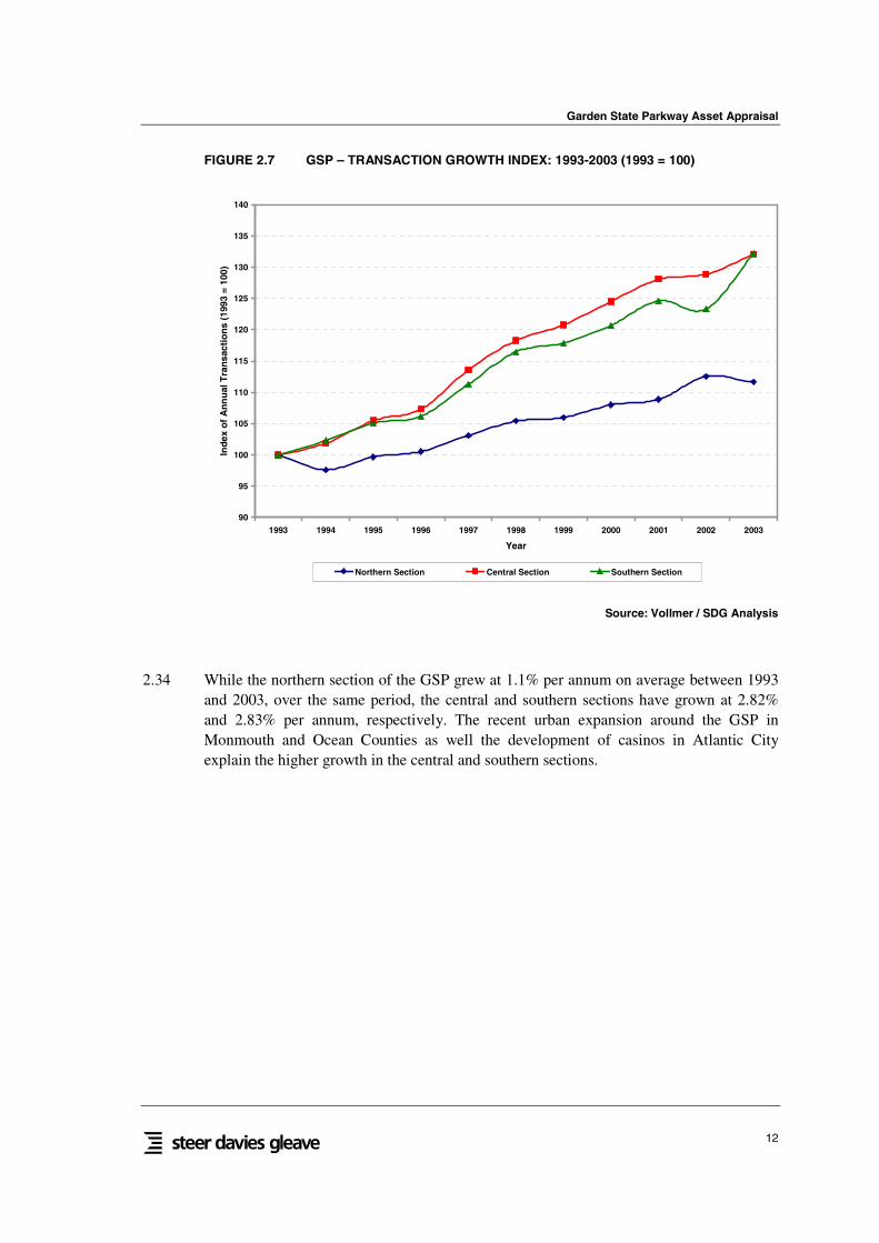
2.33 Figure 2.7 overleaf presents the development of transactions by section of road between1993 and 2003.
Garden State Parkway Asset Appraisal
12
FIGURE 2.7 GSP – TRANSACTION GROWTH INDEX: 1993-2003 (1993 = 100)
90
95
100
105
110
115
120
125
130
135
140
1993 1994 1995 1996 1997 1998 1999 2000 2001 2002 2003
Year
Ind
exo
fA
nn
ual
Tra
nsa
ctio
ns
(199
3=
100)
Northern Section Central Section Southern Section
Source: Vollmer / SDG Analysis
2.34 While the northern section of the GSP grew at 1.1% per annum on average between 1993and 2003, over the same period, the central and southern sections have grown at 2.82%and 2.83% per annum, respectively. The recent urban expansion around the GSP inMonmouth and Ocean Counties as well the development of casinos in Atlantic Cityexplain the higher growth in the central and southern sections.
Garden State Parkway Asset Appraisal
13
Toll Revenue
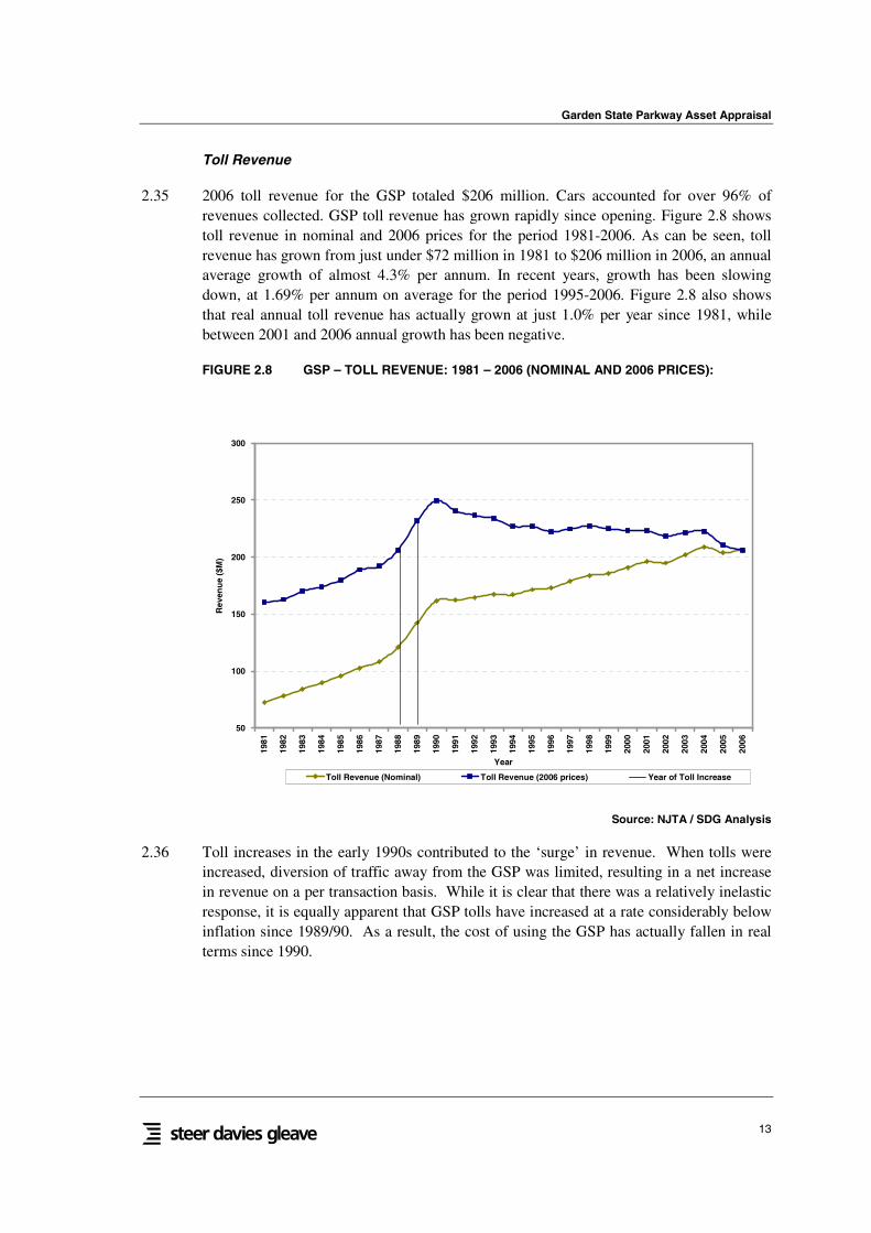
2.35 2006 toll revenue for the GSP totaled $206 million. Cars accounted for over 96% ofrevenues collected. GSP toll revenue has grown rapidly since opening. Figure 2.8 showstoll revenue in nominal and 2006 prices for the period 1981-2006. As can be seen, tollrevenue has grown from just under $72 million in 1981 to $206 million in 2006, an annualaverage growth of almost 4.3% per annum. In recent years, growth has been slowingdown, at 1.69% per annum on average for the period 1995-2006. Figure 2.8 also showsthat real annual toll revenue has actually grown at just 1.0% per year since 1981, whilebetween 2001 and 2006 annual growth has been negative.
FIGURE 2.8 GSP – TOLL REVENUE: 1981 – 2006 (NOMINAL AND 2006 PRICES):
50
100
150
200
250
300
1981
1982
1983
1984
1985
1986
1987
1988
1989
1990
1991
1992
1993
1994
1995
1996
1997
1998
1999
2000
2001
2002
2003
2004
2005
2006
Year
Rev
enu
e($
M)
Toll Revenue (Nominal) Toll Revenue (2006 prices) Year of Toll Increase
Source: NJTA / SDG Analysis
2.36 Toll increases in the early 1990s contributed to the ‘surge’ in revenue. When tolls wereincreased, diversion of traffic away from the GSP was limited, resulting in a net increasein revenue on a per transaction basis. While it is clear that there was a relatively inelasticresponse, it is equally apparent that GSP tolls have increased at a rate considerably belowinflation since 1989/90. As a result, the cost of using the GSP has actually fallen in realterms since 1990.
Garden State Parkway Asset Appraisal
14
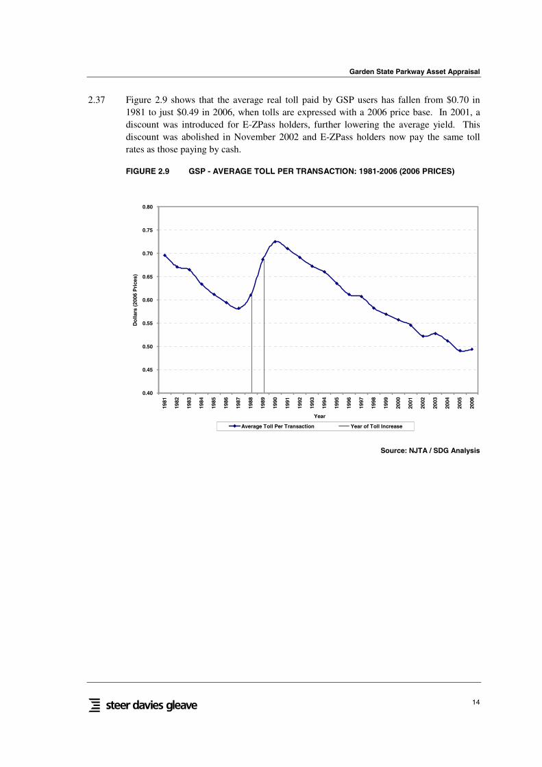
2.37 Figure 2.9 shows that the average real toll paid by GSP users has fallen from $0.70 in1981 to just $0.49 in 2006, when tolls are expressed with a 2006 price base. In 2001, adiscount was introduced for E-ZPass holders, further lowering the average yield. Thisdiscount was abolished in November 2002 and E-ZPass holders now pay the same tollrates as those paying by cash.
FIGURE 2.9 GSP - AVERAGE TOLL PER TRANSACTION: 1981-2006 (2006 PRICES)
0.40
0.45
0.50
0.55
0.60
0.65
0.70
0.75
0.80
1981
1982
1983
1984
1985
1986
1987
1988
1989
1990
1991
1992
1993
1994
1995
1996
1997
1998
1999
2000
2001
2002
2003
2004
2005
2006
Year
Do
llars
(200
6P
rice
s)
Average Toll Per Transaction Year of Toll Increase
Source: NJTA / SDG Analysis

Garden State Parkway Asset Appraisal
15
Transactions and Revenue by Vehicle Type
2.38 Table 2.4 shows the 2006 monthly revenue by vehicle type. It can be seen that theproportional split is relatively stable throughout the year.
TABLE 2.4 GSP - 2006 REVENUE BY VEHICLE TYPE ($M)
Month Cars Trucks Buses Total %Car
January 14.10 0.33 0.24 14.67 96%
February 12.99 0.31 0.22 13.52 96%
March 15.45 0.40 0.27 16.13 96%
April 15.35 0.39 0.26 16.00 96%
May 17.12 0.48 0.31 17.91 96%
June 17.81 0.49 0.29 18.59 96%
July 19.34 0.46 0.27 20.08 96%
August 19.70 0.49 0.27 20.47 96%
September 16.99 0.43 0.27 17.68 96%
October 16.92 0.44 0.28 17.64 96%
November 16.02 0.41 0.25 16.67 96%
December 16.27 0.38 0.23 16.87 96%
TOTAL 198.06 5.01 3.16 206.23 96%
Source: NJTA / SDG Analysis
Garden State Parkway Asset Appraisal
16
Transactions and Revenue by Location
2.39 Table 2.5 shows the 2006 revenue broken down by location and type of toll facility. It canbe seen that the northern section of the GSP generates around 47%, closely followed bythe central section, generating 40% of revenue. The southern end of the GSP onlyaccounts for 13% of total revenue collected.
2.40 The majority of revenue is collected at one of the mainline toll plazas. Only 22% ofrevenue is collected at the ramp plazas. Two thirds of total revenue is generated by thefollowing seven toll barriers: Raritan, Union, Asbury Park, Essex, Bergen, Toms Riverand Hillsdale.
TABLE 2.5 GSP - BREAKDOWN OF 2006 REVENUE BY SECTION AND TOLL FACILITY
Section Barrier Ramp Total
North 35.8% 11.1% 46.9%
Central 29.9% 10.1% 40.0%
South 12.1% 1.0% 13.1%
TOTAL 77.8% 22.2% 100%
Source: NJTA / SDG Analysis
2.41 In 2006, annual transactions on the GSP were highest in the northern and central sectionswhich experienced 198 and 175 million transactions. In contrast, the southern sectiononly generated 45 million transactions, representing 11% of total transactions on the GSP.
2.42 As expected, a high proportion, 88%, of total toll revenue is generated by the northern andcentral sections as shown in Table 2.6.
TABLE 2.6 GSP - 2006 ANNUAL TRANSACTIONS AND REVENUE BY SECTION
SectionTransactions
(M)% of Total
Revenue($M)
% of TotalYield ($ pertransaction)
North 197.6 47.3% 98.0 47.6% 0.50
Central 174.8 41.9% 83.5 40.5% 0.48
South 44.9 10.8% 25.7 12.5% 0.55
TOTAL 417.4 100% 206 100% 0.49
Source: NJTA / SDG Analysis
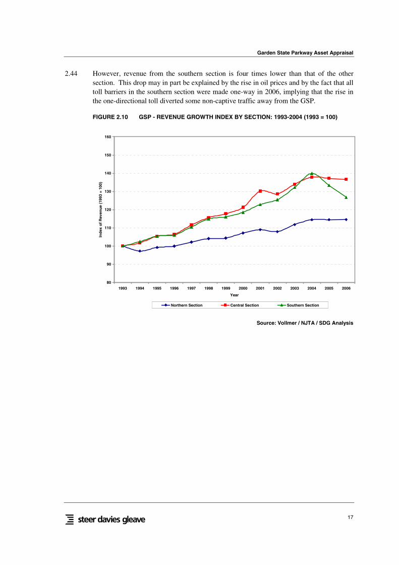
2.43 Revenue has not grown uniformly across the length of the GSP. Figure 2.10 showsindexed revenue growth between 1993 and 2006 by section of road. At the northern end,revenue grew least and slowest by 1.1% per annum, while on the central and southernsections it grew 2.4% and 1.8% per annum, respectively. The southern end displays adrop in revenue since 2005 (-4.9% per annum).
Garden State Parkway Asset Appraisal
17
2.44 However, revenue from the southern section is four times lower than that of the othersection. This drop may in part be explained by the rise in oil prices and by the fact that alltoll barriers in the southern section were made one-way in 2006, implying that the rise inthe one-directional toll diverted some non-captive traffic away from the GSP.
FIGURE 2.10 GSP - REVENUE GROWTH INDEX BY SECTION: 1993-2004 (1993 = 100)
80
90
100
110
120
130
140
150
160
1993 1994 1995 1996 1997 1998 1999 2000 2001 2002 2003 2004 2005 2006
Year
Ind
exo
fR
even
ue
(199
3=
100)
Northern Section Central Section Southern Section
Source: Vollmer / NJTA / SDG Analysis
Garden State Parkway Asset Appraisal
18
Revenue by Payment Method
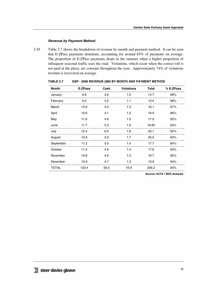
2.45 Table 2.7 shows the breakdown of revenue by month and payment method. It can be seenthat E-ZPass payments dominate, accounting for around 65% of payments on average.The proportion of E-ZPass payments drops in the summer when a higher proportion ofinfrequent seasonal traffic uses the road. Violations, which occur when the correct toll isnot paid at the plaza, are constant throughout the year. Approximately 74% of violationsrevenue is recovered on average.
TABLE 2.7 GSP - 2006 REVENUE ($M) BY MONTH AND PAYMENT METHOD
Month E-ZPass Cash Violations Total % E-ZPass
January 9.9 3.6 1.2 14.7 68%
February 9.2 3.2 1.1 13.5 68%
March 10.9 4.0 1.3 16.1 67%
April 10.6 4.1 1.3 16.0 66%
May 11.6 4.8 1.5 17.9 65%
June 11.7 5.3 1.6 18.60 63%
July 12.4 6.0 1.8 20.1 62%
August 12.9 5.9 1.7 20.5 63%
September 11.2 5.0 1.4 17.7 64%
October 11.4 4.9 1.4 17.6 64%
November 10.8 4.6 1.3 16.7 65%
December 10.9 4.7 1.3 16.9 64%
TOTAL 133.4 56.0 16.9 206.2 65%
Source: NJTA / SDG Analysis

Garden State Parkway Asset Appraisal
19
Seasonal Traffic Profiles
2.46 Figure 2.11 below shows the monthly profile of transactions volumes for three tollbarriers on the GSP.
Northern Section
2.47 At Union toll barrier, located in the Northern section of the GSP, the transactions profile isrelatively flat with equal volumes of transactions throughout the year (around 8%).
Central Section
2.48 The Central section, represented by Asbury Park toll barrier, sees a small peak of summertransactions with the months of July and August seeing higher than average transactionsvolumes (around 10% of total transactions for the year are generated in these months).The seasonality profiles imply that there are high proportions of regular users in both theNorthern and Central sections.
Southern Section
2.49 At Great Egg toll barrier, located in the Southern section of the GSP, the seasonal natureof the GSP is apparent. The peak in the number of transactions occurs between June andSeptember, during which more than half of total annual transactions are generated. Thewinter months, see a drop in the number of transactions – with only 4% of transactionsgenerated in January. The Southern section of the GSP is thus mostly used forrecreational as opposed to work related purposes.
FIGURE 2.11 GSP - MONTHLY PROFILE OF 2006 TRANSACTIONS VOLUMES
0%
2%
4%
6%
8%
10%
12%
14%
16%
JAN FEB MAR APR MAY JUN JUL AUG SEP OCT NOV DEC
Month
Pro
po
rtio
nA
nn
ual
Tra
nsa
ctio
ns
Union Asbury Park Great Egg
Source: NJTA / SDG Analysis
Garden State Parkway Asset Appraisal
20
Daily Transactions Profile
2.50 We have analyzed daily traffic profiles for typical weekday and weekend days in October2006 at main barriers along the GSP.
Northern Section
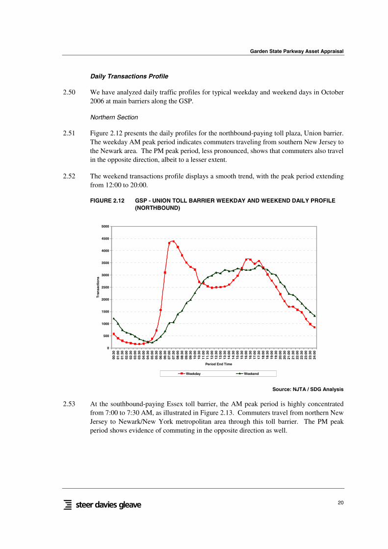
2.51 Figure 2.12 presents the daily profiles for the northbound-paying toll plaza, Union barrier.The weekday AM peak period indicates commuters traveling from southern New Jersey tothe Newark area. The PM peak period, less pronounced, shows that commuters also travelin the opposite direction, albeit to a lesser extent.
2.52 The weekend transactions profile displays a smooth trend, with the peak period extendingfrom 12:00 to 20:00.
FIGURE 2.12 GSP - UNION TOLL BARRIER WEEKDAY AND WEEKEND DAILY PROFILE(NORTHBOUND)
0
500
1000
1500
2000
2500
3000
3500
4000
4500
5000
00:3
001
:00
01:3
002
:00
02:3
003
:00
03:3
004
:00
04:3
005
:00
05:3
006
:00
06:3
007
:00
07:3
008
:00
08:3
009
:00
09:3
010
:00
10:3
011
:00
11:3
012
:00
12:3
013
:00
13:3
014
:00
14:3
015
:00
15:3
016
:00
16:3
017
:00
17:3
018
:00
18:3
019
:00
19:3
020
:00
20:3
021
:00
21:3
022
:00
22:3
023
:00
23:3
024
:00
Period End Time
Tra
nsa
ctio
ns
Weekday Weekend
Source: NJTA / SDG Analysis
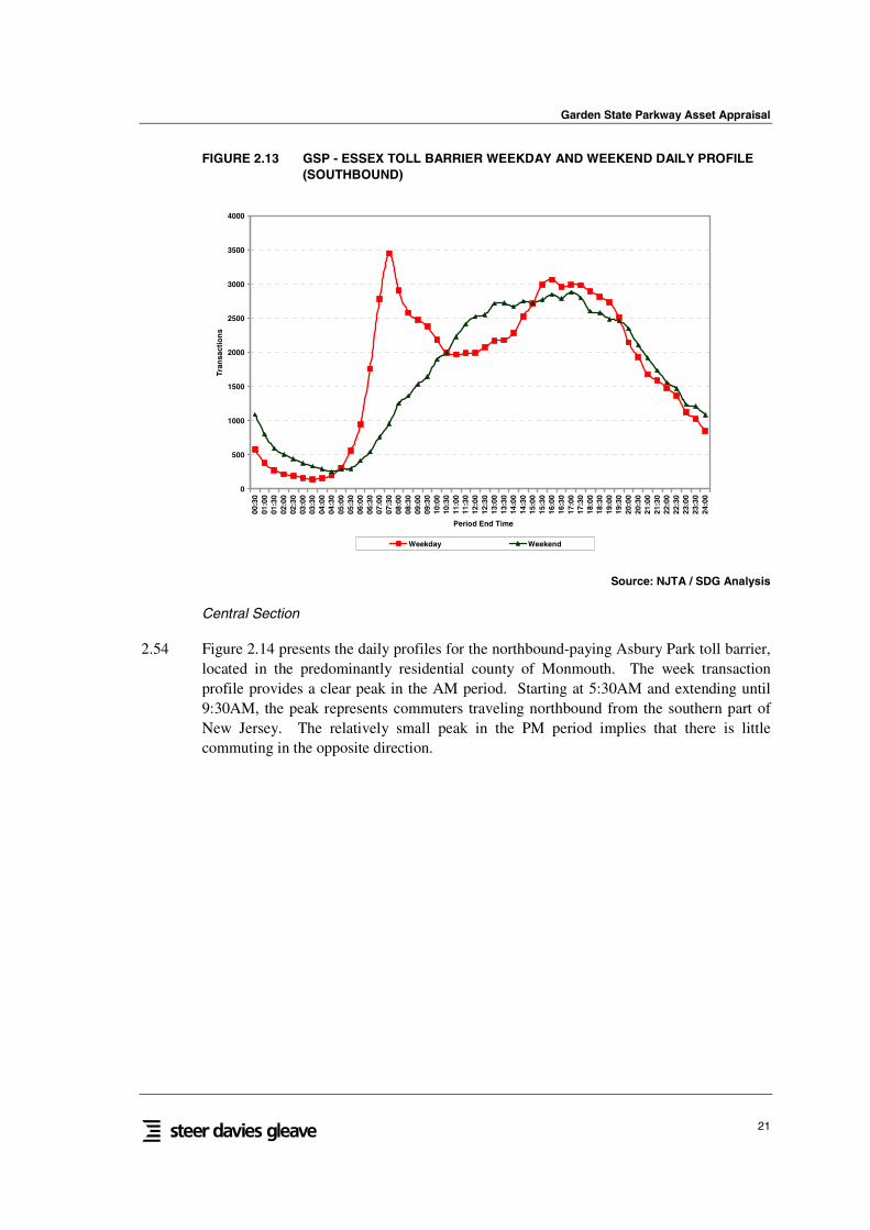
2.53 At the southbound-paying Essex toll barrier, the AM peak period is highly concentratedfrom 7:00 to 7:30 AM, as illustrated in Figure 2.13. Commuters travel from northern NewJersey to Newark/New York metropolitan area through this toll barrier. The PM peakperiod shows evidence of commuting in the opposite direction as well.
Garden State Parkway Asset Appraisal
21
FIGURE 2.13 GSP - ESSEX TOLL BARRIER WEEKDAY AND WEEKEND DAILY PROFILE(SOUTHBOUND)
0
500
1000
1500
2000
2500
3000
3500
4000
00:3
001
:00
01:3
002
:00
02:3
003
:00
03:3
004
:00
04:3
005
:00
05:3
006
:00
06:3
007
:00
07:3
008
:00
08:3
009
:00
09:3
010
:00
10:3
011
:00
11:3
012
:00
12:3
013
:00
13:3
014
:00
14:3
015
:00
15:3
016
:00
16:3
017
:00
17:3
018
:00
18:3
019
:00
19:3
020
:00
20:3
021
:00
21:3
022
:00
22:3
023
:00
23:3
024
:00
Period End Time
Tra
nsa
ctio
ns
Weekday Weekend
Source: NJTA / SDG Analysis
Central Section
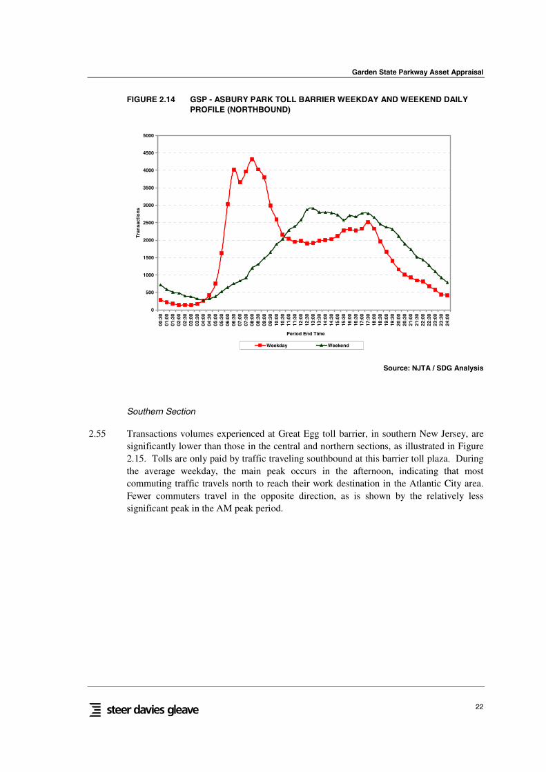
2.54 Figure 2.14 presents the daily profiles for the northbound-paying Asbury Park toll barrier,located in the predominantly residential county of Monmouth. The week transactionprofile provides a clear peak in the AM period. Starting at 5:30AM and extending until9:30AM, the peak represents commuters traveling northbound from the southern part ofNew Jersey. The relatively small peak in the PM period implies that there is littlecommuting in the opposite direction.
Garden State Parkway Asset Appraisal
22
FIGURE 2.14 GSP - ASBURY PARK TOLL BARRIER WEEKDAY AND WEEKEND DAILYPROFILE (NORTHBOUND)
0
500
1000
1500
2000
2500
3000
3500
4000
4500
5000
00:3
001
:00
01:3
002
:00
02:3
003
:00
03:3
004
:00
04:3
005
:00
05:3
006
:00
06:3
007
:00
07:3
008
:00
08:3
009
:00
09:3
010
:00
10:3
011
:00
11:3
012
:00
12:3
013
:00
13:3
014
:00
14:3
015
:00
15:3
016
:00
16:3
017
:00
17:3
018
:00
18:3
019
:00
19:3
020
:00
20:3
021
:00
21:3
022
:00
22:3
023
:00
23:3
024
:00
Period End Time
Tran
sact
ion
s
Weekday Weekend
Source: NJTA / SDG Analysis
Southern Section
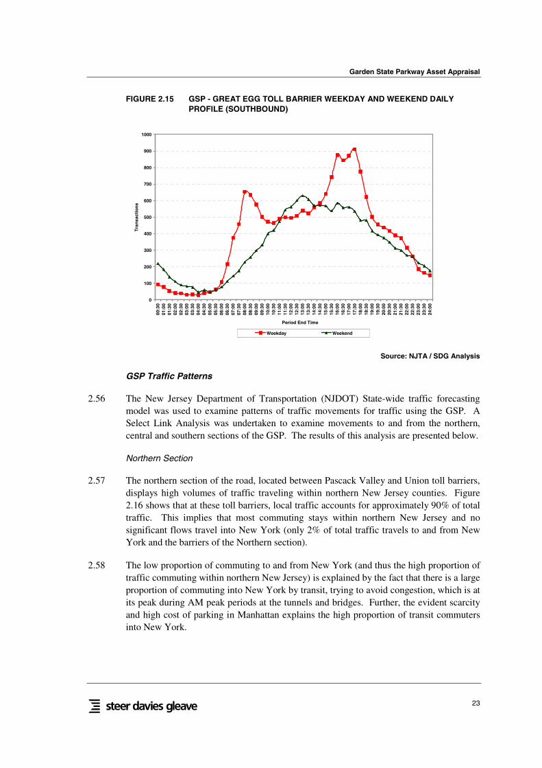
2.55 Transactions volumes experienced at Great Egg toll barrier, in southern New Jersey, aresignificantly lower than those in the central and northern sections, as illustrated in Figure2.15. Tolls are only paid by traffic traveling southbound at this barrier toll plaza. Duringthe average weekday, the main peak occurs in the afternoon, indicating that mostcommuting traffic travels north to reach their work destination in the Atlantic City area.Fewer commuters travel in the opposite direction, as is shown by the relatively lesssignificant peak in the AM peak period.
Garden State Parkway Asset Appraisal
23
FIGURE 2.15 GSP - GREAT EGG TOLL BARRIER WEEKDAY AND WEEKEND DAILYPROFILE (SOUTHBOUND)
0
100
200
300
400
500
600
700
800
900
1000
00:3
001
:00
01:3
002
:00
02:3
003
:00
03:3
004
:00
04:3
005
:00
05:3
006
:00
06:3
007
:00
07:3
008
:00
08:3
009
:00
09:3
010
:00
10:3
011
:00
11:3
012
:00
12:3
013
:00
13:3
014
:00
14:3
015
:00
15:3
016
:00
16:3
017
:00
17:3
018
:00
18:3
019
:00
19:3
020
:00
20:3
021
:00
21:3
022
:00
22:3
023
:00
23:3
024
:00
Period End Time
Tra
nsa
ctio
ns
Weekday Weekend
Source: NJTA / SDG Analysis
GSP Traffic Patterns
2.56 The New Jersey Department of Transportation (NJDOT) State-wide traffic forecastingmodel was used to examine patterns of traffic movements for traffic using the GSP. ASelect Link Analysis was undertaken to examine movements to and from the northern,central and southern sections of the GSP. The results of this analysis are presented below.
Northern Section
2.57 The northern section of the road, located between Pascack Valley and Union toll barriers,displays high volumes of traffic traveling within northern New Jersey counties. Figure2.16 shows that at these toll barriers, local traffic accounts for approximately 90% of totaltraffic. This implies that most commuting stays within northern New Jersey and nosignificant flows travel into New York (only 2% of total traffic travels to and from NewYork and the barriers of the Northern section).
2.58 The low proportion of commuting to and from New York (and thus the high proportion oftraffic commuting within northern New Jersey) is explained by the fact that there is a largeproportion of commuting into New York by transit, trying to avoid congestion, which is atits peak during AM peak periods at the tunnels and bridges. Further, the evident scarcityand high cost of parking in Manhattan explains the high proportion of transit commutersinto New York.

Garden State Parkway Asset Appraisal
24
Central Section
2.59 The central section, located between Raritan and Toms River toll barriers, displaysdecreasing volumes of traffic traveling to and from northern New Jersey as the tollbarriers are further south. Between 7 and 5% of total traffic passing through barriers ofthe central section, travel to and from New York – a higher proportion than that of thenorthern section. In this area, commuters must rely on their cars in order to reach NewYork.
Southern Section
2.60 The southern section, located between Barnegat and Great Egg toll barriers, displayssteadily decreasing volumes of traffic traveling to and from northern New Jersey as thetoll barriers are located further south. The proportion traveling to and from New Yorkremains that of the central section except at Great Egg toll barrier where virtually notraffic travels to and from New York.
FIGURE 2.16 GSP - TRAFFIC PATTERNS BY TOLL PLAZA (MODELLED)
2% 2% 1% 2%
7%5% 5% 5% 6%
1%
88%
94%92%
88%
41%
25%
17%
11%
6%
0%0%
10%
20%
30%
40%
50%
60%
70%
80%
90%
100%
Pas
cack
Val
ley
Ber
gen
Ess
ex
Un
ion
Rar
itan
Asb
ury
par
k
To
ms
Riv
er
Bar
neg
at
New
Gre
tna
Gre
atE
gg
Per
cen
tag
eo
fT
ota
lTra
ffic
To/From NY To/From Northern NJ
Source: NJDOT Model / SDG Analysis
2.61 The general pattern appears to be that the further south, the less traffic travels to and fromNorthern New Jersey. This can be explained both by the distance factor but also by theinfluences from both Atlantic City and Philadelphia on the proportion oforigins/destinations, as one would expect traffic in the southern part of New Jersey to beattracted to these employment and recreational areas. This also provides an indication ofthe low proportion of end-to-end traffic.
Garden State Parkway Asset Appraisal
25
Traffic Speeds and Congestion
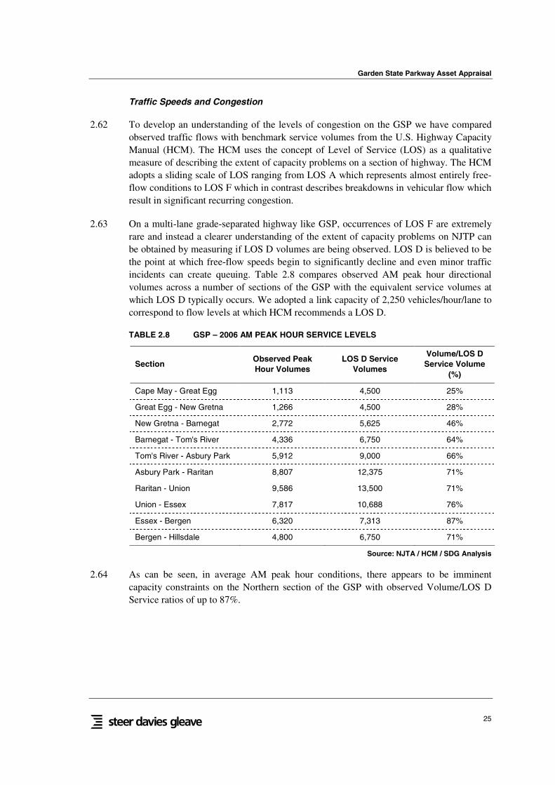
2.62 To develop an understanding of the levels of congestion on the GSP we have comparedobserved traffic flows with benchmark service volumes from the U.S. Highway CapacityManual (HCM). The HCM uses the concept of Level of Service (LOS) as a qualitativemeasure of describing the extent of capacity problems on a section of highway. The HCMadopts a sliding scale of LOS ranging from LOS A which represents almost entirely free-flow conditions to LOS F which in contrast describes breakdowns in vehicular flow whichresult in significant recurring congestion.
2.63 On a multi-lane grade-separated highway like GSP, occurrences of LOS F are extremelyrare and instead a clearer understanding of the extent of capacity problems on NJTP canbe obtained by measuring if LOS D volumes are being observed. LOS D is believed to bethe point at which free-flow speeds begin to significantly decline and even minor trafficincidents can create queuing. Table 2.8 compares observed AM peak hour directionalvolumes across a number of sections of the GSP with the equivalent service volumes atwhich LOS D typically occurs. We adopted a link capacity of 2,250 vehicles/hour/lane tocorrespond to flow levels at which HCM recommends a LOS D.
TABLE 2.8 GSP – 2006 AM PEAK HOUR SERVICE LEVELS
SectionObserved PeakHour Volumes
LOS D ServiceVolumes
Volume/LOS DService Volume
(%)
Cape May - Great Egg 1,113 4,500 25%
Great Egg - New Gretna 1,266 4,500 28%
New Gretna - Barnegat 2,772 5,625 46%
Barnegat - Tom's River 4,336 6,750 64%
Tom's River - Asbury Park 5,912 9,000 66%
Asbury Park - Raritan 8,807 12,375 71%
Raritan - Union 9,586 13,500 71%
Union - Essex 7,817 10,688 76%
Essex - Bergen 6,320 7,313 87%
Bergen - Hillsdale 4,800 6,750 71%
Source: NJTA / HCM / SDG Analysis
2.64 As can be seen, in average AM peak hour conditions, there appears to be imminentcapacity constraints on the Northern section of the GSP with observed Volume/LOS DService ratios of up to 87%.

Garden State Parkway Asset Appraisal
26
2.65 Table 2.9 shows average AM peak hour speeds on a number of sections.
TABLE 2.9 GSP - AM PEAK PERIOD SPEEDS
Section Northbound Speed (mph) Southbound Speed (mph)
Tom's River - Asbury Park 68.6 63.3
Asbury Park - Raritan 65.8 72.1
Raritan - Union 51.7 65.1
Union - Essex 45.0 63.0
Essex - Bergen 47.1 51.2
Bergen - Hillsdale 56.6 61.9
Source: SDG Analysis
2.66 As can be seen, traffic speeds are typically above 50 mph during the AM peak hourperiod. Speeds are lower in the northern section of the road between Union and Hillsdalewhere the route passes through the Newark metropolitan area but this is likely to be areflection of the lower 55 mph speed limit in this area rather than the effect significantcapacity constraints.
2.67 Table 2.10 provides equivalent analysis for the off-peak period. Here speeds are almost atcompletely free-flow conditions indicating very few or no capacity constraints in the offpeak.
TABLE 2.10 GSP - OFF PEAK SPEEDS
Section Northbound Speed (mph) Southbound Speed (mph)
Tom's River - Asbury Park 68.6 64.5
Asbury Park - Raritan 71.2 69.1
Raritan - Union 68.5 66.0
Union - Essex 65.9 67.1
Essex - Bergen 64.7 62.3
Bergen - Hillsdale 59.5 64.5
Source: SDG Analysis
Behavioral Research
2.68 As part of our literature review we concluded that it would be worthwhile undertakingfieldwork to compare the markets served by the three roads of interest, and possibly alsoto gather evidence on other key issues that the modeling process should address.
Garden State Parkway Asset Appraisal
27
2.69 A survey was undertaken to provide fresh evidence on certain key issues of relevance tothe study. As part of the survey, 395 GSP users were interviewed between Friday 16th
March and Tuesday 20th March 2007. Further details of the survey methodology andanalysis can be found in Appendix C of the Background Report, Behavioral Research.
2.70 GSP users, like the users of the NJTP, are not very sensitive to the price of the tolls - atleast not at their present level, which is low compared to other toll roads in the UnitedStates. While GSP users are undoubtedly sensitive to the idea of the tolls going up, thesurvey presents an accumulation of findings which show that at present many of them donot worry about the price of the tolls.
2.71 The GSP users set themselves apart from users of the other roads in that they seem to beeven more car-dependent (87% agreed with the statement that for most of their trips theyhad no choice but to drive), they were more likely to say that the road is essential to themtraveling around NJ (67% agreed), and they were also more likely to agree with thesentiment that it is unfair to charge for using the road (45% agreed). There seems to bemore of a feeling that the GSP should be a public service amongst the frequent users ofthe road, compared to the users of the NJTP and the users of the ACE.
2.72 The GSP users had an income profile broadly similar to that of the NJTP users, but with alower proportion of people in the highest income bracket - only a quarter of GSP usersclassified themselves in this category, compared to a third of the NJTP users. Of the GSPusers, 70% lived in NJ, 24% in New York, and the remainder in the adjoining states ofPennsylvania, Delaware and Connecticut.
2.73 In terms of the perceived value for money, level of congestion, and the stress of using theroad, the GSP users had slightly less negative experiences than the NJTP users, butsignificantly more negative experiences than the ACE users. The more significantfindings were that 51% of the GSP users described the value for money of the tolls asbeing “average”, 60% of them said that they did not normally think about how much theyspend on tolls, and congestion did not feature as a significant reason for using the roadless.
2.74 The GSP users’ evaluation of the importance of their most recent trip on the GSP wasvery similar to that of the NJTP users’ regarding the NJTP: both these groups of usersregarded their most recent trip using the respective road as being more important,compared to the ACE users’ evaluation of the importance of their recent trips on the ACE.GSP users were more likely to consider alternative routes compared to the NJTP users, butless likely to consider alternative routes in comparison to the ACE users. GSP users wereless likely to consider other modes of transport, compared to users of the NJTP.
Garden State Parkway Asset Appraisal
28
2.75 About 60% of GSP users with EZ-Pass do not normally think about the cost of using theroad - even more than in the case of NJTP users (50%), but less than in the case of ACEusers (70%). The evidence on value of time showed that the proportion of people withmedium or high values of time was lower for the GSP users compared to the NJTP users -the distribution of values of time for GSP users was very similar to that of the ACE users.The direct questions about toll price changes suggested that in terms of the likelihood ofthem changing their behavior in response to a toll rise, the GSP users fall between theNJTP users (expected to be least responsive) and the ACE users (expected to be mostresponsive).
2.76 Individuals did not report significant changes in their usage of the toll roads, and thereasons given for changes in usage were dominated by changes in personal circumstances.The evidence suggests that there has been no significant change to the level of congestionon the GSP over the last 2 years – about half the respondents reported that the congestionthey experienced on the GSP had not changed, and the remainder was split more or lessevenly between reporting improvement and reporting deterioration.
2.77 When asked about changes to the tolls over the past two years (there have not been anysignificant changes), only about 63% of the GSP users correctly answered that the tollshad not changed (or said they were not sure) - most of the rest responded that the tolls hadgone up, with 4% saying that “tolls are now much higher” compared to two years ago.This adds to the impression that many GSP users do not have a clear idea of how muchthey are paying and whether or not it has been changing.
2.78 The survey suggests that the gasoline price rises over the past two years have not had asignificant impact on people’s use of the GSP, and that many people would adapt to futuregas price increases by switching to vehicles with greater fuel-efficiency.
Garden State Parkway Asset Appraisal
29
Summary
• The GSP is a 173 mile long toll road stretching along the New Jersey shoreline. Itserves as a primary link along the coast, serving seashore recreational areas, AtlanticCity and the Newark/New York metropolitan area;
• Heavy Trucks (registered 7,000 lbs. or more) are prohibited north of Exit 105;
• The facility intersects with the major highway routes within New Jersey including theACE and NJTP providing access to New York City;
• The GSP is a grade-separated limited access interstate-standard facility with a speedlimit ranging from 55-65 mph. The number of lanes range from two per direction inthe south of the facility to six lanes per direction in the northern sections;
• A number of competing routes exist along the length of the GSP. In the North (Exit172 to Exit 127) it competes with the I-287 and NJTP. In the South, US-9 competeswith the GSP for short distance journeys;
• The GSP operates as an ‘open system’ whereby users pay tolls at regular intervalsalong the length of the road and at certain exits. On some short distance sections,vehicles can use the road without paying tolls;
• The GSP is an existing road and has been open for decades. As a result we haveprecise knowledge about the amount of traffic that is currently carried by the roadand how much toll revenue is collected;
• Historic transaction data allows us to consider how traffic levels have changed overtime, how traffic has responded in the past to changes in toll rates and what therelation between traffic on the GSP and past economic growth has been;
• With a cost-per-mile rate of approximately $0.02 per mile, the GSP is currently theleast costly toll road in the United States. Payment can be made in cash or by E-ZPass - the ETC system in place on the facility;
• In 2006 there were over 417 million toll transactions on the GSP, this is equivalent tojust over 1.1 million transactions per day on average. Cars accounted for 96% oftransactions, whereas trucks and buses accounted for the remaining 4%;
• Between 1981 and 2006 toll revenue has grown at 4.3% on average from $72 millionto $206 million. However toll revenue in real terms has only grown at 1.0% per yearover the same period;
Garden State Parkway Asset Appraisal
30
• The northern section of the GSP generates around 47% of revenue, closely followedby the central section, generating 40% of revenue. The southern end of the GSP onlyaccounts for 13% of total revenue collected;
• Traffic growth has been most rapid in the central and southern section of the route,while growth in the north of the facility has recently stagnated – a possible cause ofwhich is the growing congestion and capacity problems in this section;
• GSP tolls have increased at a rate considerably below inflation since 1989/90. As aresult, the cost of using the GSP has actually fallen in real terms from $0.70 in 1981to just $0.49 in 2006 (2006 prices);
• E-ZPass payments dominate, accounting for around 65% of payments. Theproportion of E-ZPass payments drops in the summer when a higher proportion ofinfrequent seasonal traffic uses the road;
• Capacity constraints are evident as the route reaches the Newark metropolitan areaswhere traffic flows will typically reach in excess of 200,000 vehicles per day andaverage daily speeds can reach as low as 30 mph in peak periods; and
• The obvious congestion in the northern section of the facility appears to haveproduced ‘peak spreading’ with peak conditions observed for several hours in themorning and evening peaks.
• A key issue for the GSP concession is to understand how traffic levels will bechanging over time and what the impact of capacity constraints are. Important inputsinto this process are assumptions with regards to economic growth, population, andmajor developments (mainly port and infrastructure) that are planned to take place inthe study area or surroundings and that may impact on traffic levels.
Garden State Parkway Asset Appraisal
31
3. THE FORECASTING METHODOLOGY
Introduction
3.1 We have developed a modeling framework that can explore the base assignment to thetarget facility under a range of scenarios – and for different traffic types. The key issue forthe GSP concession is to understand how traffic levels will be changing over time andwhat the impact of capacity constraints are. Important inputs into this process areassumptions with regards to economic growth, population, and major developments(mainly port and infrastructure) that are planned to take place in the study area orsurroundings and that may impact on traffic levels.
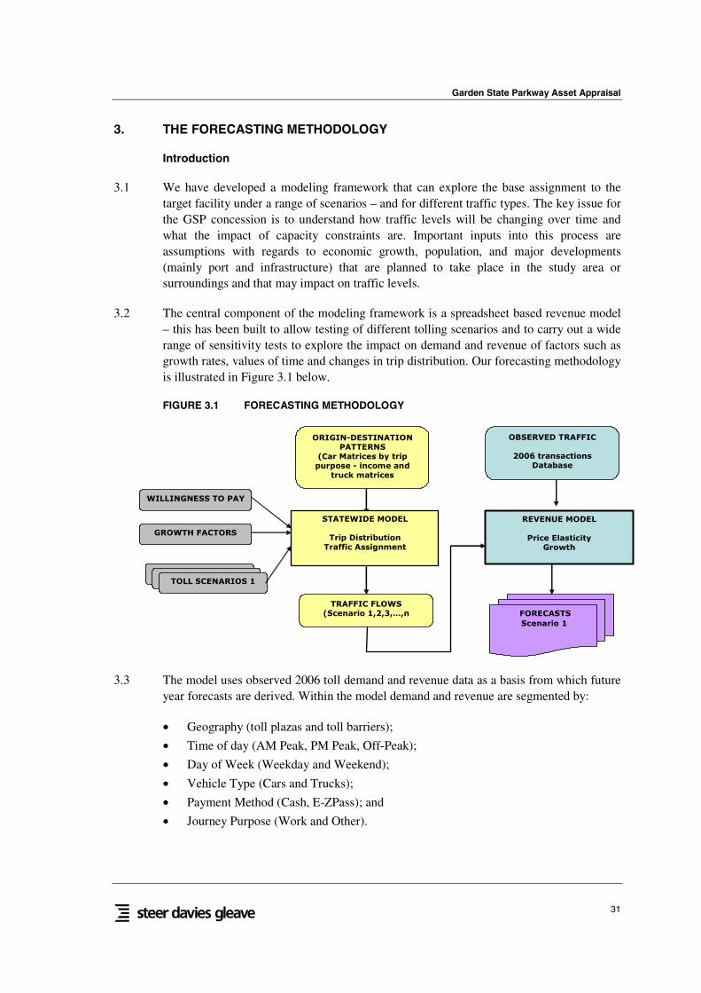
3.2 The central component of the modeling framework is a spreadsheet based revenue model– this has been built to allow testing of different tolling scenarios and to carry out a widerange of sensitivity tests to explore the impact on demand and revenue of factors such asgrowth rates, values of time and changes in trip distribution. Our forecasting methodologyis illustrated in Figure 3.1 below.
FIGURE 3.1 FORECASTING METHODOLOGY
STATEWIDE MODEL
Trip DistributionTraffic Assignment
TRAFFIC FLOWS (Scenario 1,2,3,…,n
REVENUE MODEL
Price Elasticity Growth
WILLINGNESS TO PAY
FORECASTSScenario 1
ORIGIN-DESTINATION PATTERNS
(Car Matrices by trip purpose - income and
truck matrices
GROWTH FACTORS
TOLL SCENARIOSTOLL SCENARIOS 2TOLL SCENARIOS 1
OBSERVED TRAFFIC
2006 transactions Database
3.3 The model uses observed 2006 toll demand and revenue data as a basis from which futureyear forecasts are derived. Within the model demand and revenue are segmented by:
• Geography (toll plazas and toll barriers);
• Time of day (AM Peak, PM Peak, Off-Peak);
• Day of Week (Weekday and Weekend);
• Vehicle Type (Cars and Trucks);
• Payment Method (Cash, E-ZPass); and
• Journey Purpose (Work and Other).
Garden State Parkway Asset Appraisal
32
3.4 We have adopted a number of existing modeling tools to inform the revenue model interms of:
• Impact of congestion;
• Changes in trip distribution;
• Diversion; and
• Traffic Growth.
3.5 The network models used are an updated version of the State-wide model, which wasinitially developed over 10 years ago as an all day (24 hour) traffic assignment model.For the purpose of our assignment, we have updated the trip tables, road network (baseand future) and assignment procedures.
3.6 The trip tables were updated with the information on trip patterns (Origin- Destinationand Journey Purpose split by time of the day) from the NJTPA and SJTPO. Car trips weresegmented into two journey purposes (home based work and other), with both journeypurposes split into four income groups. The four income groups are based on county-levelCensus 2000 household income levels that fit into the income ranges of the four incomegroups identified in the NJTPA (values grown to 2000). Commercial vehicles were treatedas one segment.
3.7 The road network for the area comprises the freeway, arterial and collector facilities.Each road link contains information on the number of lanes, free flow speeds, capacity,volume-delay relationships and toll charges at toll plazas. The link characteristics wereupdated to reflect coding of the NJTPA and SJTPO networks for significant roads. Also afuture 2025 year network was built which incorporates those planned infrastructureimprovements in the New Jersey area that could have a significant impact on the roadnetwork.
3.8 The link volume-delay relationships and factors to convert hourly capacity into each timeperiod were reviewed and updated using recent traffic count travel time data collectedspecifically for the purpose of this assignment. The re-calibrated volume delay functionsprovided a significantly improved fit to the observed travel time data.
3.9 The third component is the assignment process used to estimate how origin-destinationdemand will route itself over the available network facilities. The vehicle (auto and truck)assignments are based on a process that iterates until network or passenger travel times arein equilibrium. The resulting outputs include vehicle (auto and truck) network volumes,travel times and costs.
Garden State Parkway Asset Appraisal
33
Impact of Toll Changes and Congestion
3.10 There are several ways in which people can adapt to a change in toll levels and increasedlevels of congestion, as follows:
• Time period - in the case of relative changes in the tolls applying to specific timeperiods or congestion occurring at specific times;
• Route - in many cases, however, alternative routes offer considerably longer andmore uncertain journey times;
• Vehicle occupancy - ride sharing can reduce the trip costs per passenger / reducecongestion;
• Mode - flying for long-distance through passenger traffic, rail for certain otherOrigin-Destination (O-D) combinations (the NJ Transit rail network focuses on tripsto and from New York);
• Destination - in some cases people might consider going to a different city if there isa big difference in the cost of the trip or congestion levels; and
• Activity - some people might offset the higher costs of travel by doing the activityless often, or not at all.
3.11 Recent research by Ozbay1 et al. on the behavioral response to the time of day pricinginitiative on the NJTP showed that the most common responses to increased peak-hourtolls and reduced off-peak tolls were to travel by alternative routes, to reduce use of theTurnpike, to increase ride sharing, and to increase travel in off-peak periods. However itis important to note that approximately 93% of individuals did not change their travelbehavior at all in response to the changes to the toll schedule in the year 2000. Theresearch concluded that faced by a small differential between peak and off-peak tollsbeing introduced, the demand was very inelastic.
3.12 Our modeling framework currently handles route choice and changes in travel times. Tripsuppression is due to changes in vehicle occupancy, mode-shifting, destination andactivity changes are not currently modeled explicitly, but we do allow for trip suppressiondue to capacity constraints. However we have checked the implied elasticities from themodel are reasonable compared to evidence from other roads.
1 Ozbay, K., J. Holguín-Veras, O. Yanmaz-Tuzel, S. Mudigonda, A. Lichtenstein, M. Robins, B. Bartin, M. Cetin, N. Xu,J.C. Zorrilla, S. Xia, S. Wang, and M. Silas (2005). 'Evaluation Study of New Jersey Turnpike Authority's Time-ofday Pricing Initiative'. Publication FHWA-NJ-2005-012.FHWA, U.S. Department of Transportation. Availableonline at time of writing:
http://knowledge.fhwa.dot.gov/cops/hcx.nsf/All+Documents/BA2414CE1EAC182685256DC500674090/$FILE/njtpa_fin
al_report_may_31_2005.pdf
Garden State Parkway Asset Appraisal
34
Existing and Future Capacity Constraints
3.13 Initially a set of constrained traffic forecasts was developed. These were then used todetermine when lane expansions may be required over the life of the concessions of thefour road assets. The basis for this was the requirement specified by the State that ServiceLevels should not fall below “LOS D”. Our method for estimating capacity constraints isoutlined below.
3.14 Firstly the 2006 transactions database was used to establish annual average weekdaytraffic flows (AADTw’s) by section of road, time of day and direction of travel.
3.15 From this the number of vehicles per hour per lane for each road section for the AM Peakperiod (defined as 6:00AM-9:00AM on weekdays) was derived. Traffic growth estimatesfrom the forecasting model were applied to derive this information for each of theforecasting years.
3.16 Secondly on the basis of the HCM and speed/flow relationships calibrated on other inter-urban highways, we adopted a link capacity of 2,250 vehicles/hour/lane to correspond toflow levels at which HCM recommends a LOS D2.
3.17 When forecast traffic levels exceeded the Service Level D definition capacity constrainsare believed to be binding and an expansion of one lane per direction has been assumed.The triggered expansions are summarized in Appendix C. It can be seen that for certainroad sections a secondary expansion has been necessary due to further traffic growth.Finally the traffic models were rerun to include the additional network capacities.
2 Our analysis is fully reliant on data supplied by NJDOT and its agencies, and is based on ‘average’ traffic conditions. Itis however apparent that at certain times of the year and on certain days, volumes will be considerably higher thanthese averages. In addition unforeseen incidents may generate a severe breakdown in flow and these effects will be‘smoothed’ by taking an average approach. However we feel this is the only method by which we can obtain anaccurate picture of the performance of a facility over an extended period of time and thus a fair assessment ofwhether an expansion is genuinely required. The method applied is a ‘link-based’ assessment, i.e. it does notexplicitly consider the capacity of interchanges or the interaction of the facilities with the ‘secondary’ highwaynetwork (from where downstream queuing often occurs because capacity is typically much less). By assessingconstraints purely on the basis of link volumes and capacities we are effectively isolating highway sections wherethe provision of additional lane capacity will help solve prevailing congestion levels.
Garden State Parkway Asset Appraisal
35
4. TRAFFIC GROWTH
Introduction
4.1 To derive the extent to which traffic will grow in the future, we have undertaken thefollowing:
• Reviewed the extent of economic development in the region and derived appropriate‘economic’ forecasts (e.g. we have used various recognized economic forecastingsources to derive population and employment forecasts at a county level – based ondiscussions with development agencies, we have also provided an ‘overlay’ to theseforecasts, depending on the extent new sites and developments will generateadditional population);
• Analyzed the extent to which travel-related parameters such as trip making by drivershave changed over time (e.g. there is considerable evidence from official New Jerseystatistics that drivers are undertaking more mileage every year. For the appropriatetraffic categories, we have therefore adjusted the county-based economic forecastsaccordingly to reflect this); and
• So that the growth vectors can be incorporated into the traffic modeling framework,matrices containing vectors at the county level have been developed for each of thethree traffic categories. These reflect assumptions about growth to/from origins anddestinations. The growth vector matrices then form an input to the traffic models.
4.2 As discussed in this chapter, observed economic and traffic growth in New Jersey havebeen robust and based on our review of all available data and forecasts, we believe thatthese robust level of growth will continue into the future.
Economic Development
4.3 New Jersey is a key region of economic activity within the United States and is situated atthe centre of a metropolitan axis stretching from Washington, DC to Boston, MA. TheState is the most densely populated in the United States, at 1,174 residents per squaremile. According to the United States Census Bureau, it is also the second wealthiest stateper capita in the United States.
4.4 According to the US Bureau of Economic Analysis, the State’s median household incomeis the highest in the nation, at $55,146 and it is ranked second in the nation by the numberof locations with per capita incomes above the national average of 76.4%. Nine of NewJersey's counties are in the wealthiest 100 of the country.
4.5 New Jersey has an extensive industrial base that comprises the following:
• The Port Newark-Elizabeth Marine Terminal is one of the world's largest containerports while Newark Liberty International Airport is ranked seventh among thenation's busiest airports and among the top 20 busiest airports in the world;
Garden State Parkway Asset Appraisal
36
• New Jersey’s industrial outputs include pharmaceutical and chemical products, foodprocessing, electric equipment, printing and publishing, and tourism. Additionally,New Jersey is home to the largest petroleum containment/storage system outside ofthe Middle East;
• New Jersey hosts several business headquarters (fifty Fortune 500 companies haveheadquarters in or conduct business from Morris County alone);
• New Jersey has several oil refineries and chemical plants;
• Its agricultural outputs are numerous and include nursery stock, horses, vegetables,fruits and nuts, seafood and dairy products.
4.6 It is these types of activities that generate significant volumes of traffic on the toll roads inNew Jersey. In addition, considerable volumes of car journeys are generated from thelarge number of residential developments throughout the States as well as the car tripsgenerated by the employment in major centers such as New York City.
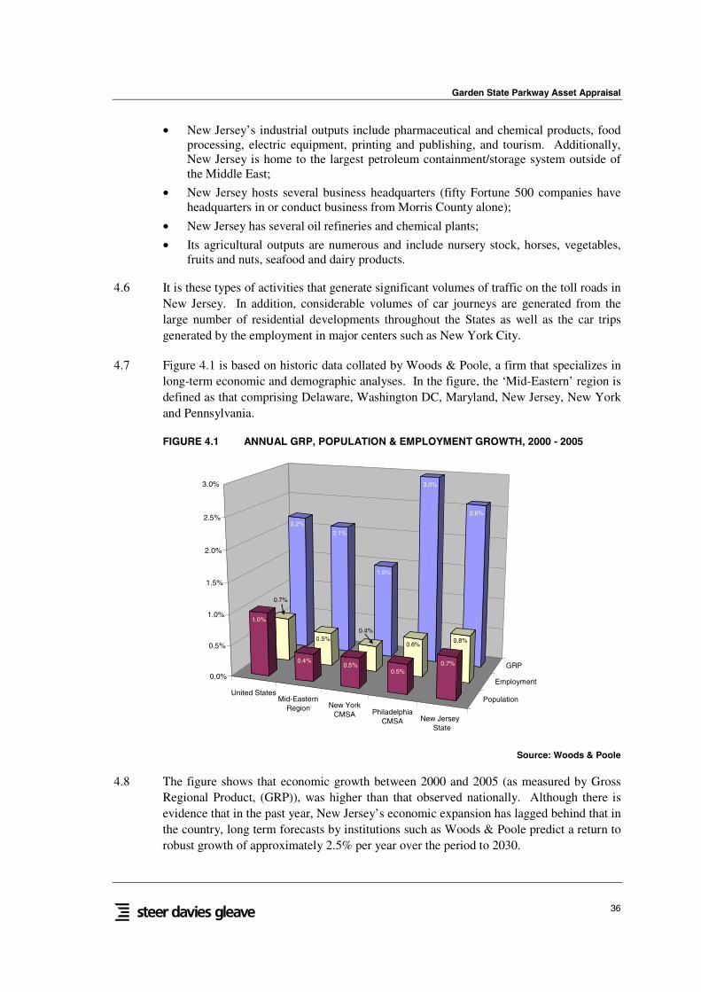
4.7 Figure 4.1 is based on historic data collated by Woods & Poole, a firm that specializes inlong-term economic and demographic analyses. In the figure, the ‘Mid-Eastern’ region isdefined as that comprising Delaware, Washington DC, Maryland, New Jersey, New Yorkand Pennsylvania.
FIGURE 4.1 ANNUAL GRP, POPULATION & EMPLOYMENT GROWTH, 2000 - 2005
United StatesMid-Eastern
Region New YorkCMSA Philadelphia
CMSA New JerseyState
Population
Employment
GRP
2.2%
2.1%
1.5%
3.0%
2.6%
0.7%
0.5%0.4%
0.6%0.8%
1.0%
0.4%0.5%
0.5%0.7%
0.0%
0.5%
1.0%
1.5%
2.0%
2.5%
3.0%
Source: Woods & Poole
4.8 The figure shows that economic growth between 2000 and 2005 (as measured by GrossRegional Product, (GRP)), was higher than that observed nationally. Although there isevidence that in the past year, New Jersey’s economic expansion has lagged behind that inthe country, long term forecasts by institutions such as Woods & Poole predict a return torobust growth of approximately 2.5% per year over the period to 2030.
Garden State Parkway Asset Appraisal
37
4.9 The figure above also shows that over the period between 2000 and 2005, employmentgrowth in New Jersey has exceeded that observed nationally while population growth hasalso been significant and has compared well with the national average.
4.10 Recent research by the Rutgers State University of New Jersey’s Economic AdvisoryService (RECON) supports the predictions of other forecasters, such as Woods & Poole,by indicating that over the longer term (between 2005 and 2016), economic growth in theState will continue to be robust.
4.11 The RECON forecasts of January 2007, for example, suggest that output in the State ofNew Jersey will increase by 2.5% per year (similar to the growth indicated in the Woods& Poole forecasts). This is an issue that has relevance to traffic growth forecasts andthese are discussed later.
Trip Rates
4.12 In addition to evaluating forecast economic and demographic growth at the county level,we have also undertaken research into the following:
• The extent of any ‘decoupling’ between economic and traffic growth; and
• Investigating whether there is evidence of an increase in VMT per capita.
4.13 These are important parameters since they provide guidance as to whether thedemographic growth-based vectors should be adjusted to reflect observed changes in tripmaking and vehicle mileage.
4.14 One of the key issues here is the evidence of any increase in annual vehicle mileage permember of the population in New Jersey. If, for example, the number of miles eachperson travels is increasing each year, this indicates that an allowance should be made forthis within any demographics-based growth vectors.
Garden State Parkway Asset Appraisal
38
Decoupling of Economic & Traffic Growth
4.15 Research undertaken in the United States (‘Decoupling Economic Growth & TransportDemand: A Requirement For Sustainability’, R Gilbert & K Nadeau, May 2002) hasshown that there is some evidence of ‘decoupling’ of economic growth and traffic growth.This is indicated in Figure 4.2 below (albeit with data only available up to 1998).
FIGURE 4.2 DECOUPLING OF ECONOMIC & TRAFFIC GROWTH 1960 – 1998 (USA)
0
50
100
150
200
250
300
350
400
1960
1961
1962
1963
1964
1965
1966
1967
1968
1969
1970
1971
1972
1973
1974
1975
1976
1977
1978
1979
1980
1981
1982
1983
1984
1985
1986
1987
1988
1989
1990
1991
1992
1993
1994
1995
1996
1997
1998
Year
Ind
ex(1
960
=10
0)
Passenger Kilometers Traveled Tonnes Kilometers Traveled Gross Domestic Product
Source: US Bureau of Transport Statistics (‘National Transport Statistics’) / US Bureau of Economic Analysis(‘Current Account Data’)
4.16 As Figure 4.2 indicates, although the motorized movement of people in the US has closelymatched the growth in the economy, there has been some decoupling of economic activityand freight transport activity since the early/mid 1970s and of economic activity andpassenger transport since the early 1990s.
4.17 Private motoring data from the New Jersey Department of Labor and WorkforceDevelopment and the Federal Transit Administration’s National Transit Database (for1997 to 2004) shows that for every $1,000 of Gross State Product, total mileage drivendecreased by approximately 5% over the period. This is indicated in Figure 4.3.

Garden State Parkway Asset Appraisal
39
FIGURE 4.3 PRIVATE VEHICLE MILES DRIVEN PER $1,000 GROSS STATE PRODUCT,NEW JERSEY, 1997-2004
180
185
190
195
200
205
1997 1998 1999 2000 2001 2002 2003 2004
Year
Mile
sD
rive
n-
Pri
vate
Veh
icle
s
Source: NJ Dept of Labor & Workforce Development, 1997-2004
4.18 For passenger mileage, although this indicates some decoupling of economic activity fromtransport activity, the annual extent of this (-0.7% per annum) is relatively small and mayreflect factors such as growth in transit use State-wide as well as a 13.6% increase in‘output per worker’ over the same period. This indicates that fewer workers (and fewerdrivers) are required to produce a larger Gross State Product.
4.19 Given this relatively small level of ‘decoupling’ each year, we have not adjusted the cartraffic growth vectors as there is considerably more evidence (see below) that on a percapita basis, drivers in New Jersey have been traveling increasing vehicle mileages eachyear.
4.20 For truck freight traffic in New Jersey, the outcome appears to be different as on average,the number of miles driven per $1,000 of Gross State Product has increased over theperiod by almost 18%. Figure 4.4 overleaf indicates this trend, including the two yearswhere the volume of mileage per Gross State Product decreased.

Garden State Parkway Asset Appraisal
40
FIGURE 4.4 TRUCK VEHICLE MILES DRIVEN PER $1,000 GROSS STATE PRODUCT,NEW JERSEY, 1997-2004
10
11
12
13
14
15
16
17
18
19
20
1997 1998 1999 2000 2001 2002 2003 2004
Year
Mile
sD
rive
n-
Tru
ckF
reig
ht
Source: NJ Dept of Labor & Workforce Development, FTA National Transit Database, 1997-2004
4.21 For truck traffic, although we have not made a direct upward adjustment to reflect thisincreased level of mileage per unit of economic activity, the growth vectors derived forthis traffic category are higher than those for other traffic types are due, in part, to thisphenomenon.
4.22 To demonstrate the high level of truck traffic observed in New Jersey between 1997 and2004, data from NJDOT’s ‘Travel Activity by Vehicle Type’ shows that truck travel grewby 44%, compared to 15% for all vehicles. Trucks traveled more than 6.3 billion miles in2004, up nearly 2 billion miles from 1997. Trucks also made up a growing share of thevehicles on New Jersey's roadways. In 2004, trucks comprised almost 9 percent of thetotal miles traveled, up from 7 percent in 1997, an increase of 25%.
Evidence of Increases in VMT Per Capita Over Time
4.23 Data collected for New Jersey indicates that there has been a steady increase in VMT percapita over time. Using both FHWA and Census data from 1975 through to 2002, therehave been several trends over different periods in the VMT per capita relationship asindicated in Figure 4.5.
Garden State Parkway Asset Appraisal
41
FIGURE 4.5 SUMMARY OF VEHICLE MILES TRAVELED PER CAPITA, 1975 - 2002
6,000
6,500
7,000
7,500
8,000
8,500
1975
1976
1977
1978
1979
1980
1981
1982
1983
1984
1985
1986
1987
1988
1989
1990
1991
1992
1993
1994
1995
1996
1997
1998
1999
2000
2001
2002
Year
Mile
sp
erY
ear
per
Per
son
Source: NJDOT (figure produced in New Jersey Department of Environment Protection’s
‘Environmental Trends 2005’)
4.24 As the figure shows, there are several distinct ‘periods’ in which the relationship betweenvehicle mileage per person changes and these are summarized below:
• 1975 – 1980: a period of comparatively strong growth (despite downturn in 1979);
• 1980 – 1985: VMT per capita remained broadly constant;
• 1985 – 1989: VMT per capita increased by just over 2% per annum;
• 1989 – 1995: VMT per capita fell; and
• 1995 – 2005: VMT per capita increased by just over 1% per annum.
4.25 The most important conclusion to be drawn from the data in the figure is that there hasbeen a steady increase in miles per capita since the mid-1990s. Following the end of theeconomic downturn of the early 1990s, drivers throughout New Jersey have beenundertaking more mileage each year as their need to travel increases.
4.26 Over the last five years, for example, the average increase has been approximately 1.2%per annum. In other words, New Jersey residents are driving approximately 1.2% moremiles compared to the previous year.
Garden State Parkway Asset Appraisal
42
4.27 Figure 4.6 shows the absolute vehicle miles traveled per capita between 2000 and 2005.The figure clearly indicates that although VMT per capita decreased between 2002 and2003, this was more than made up in the following year. The decrease between theseyears is most likely, however, to be attributed to the ‘one off’ economic shock associatedwith the events of 9/11. We would thus conclude from the longer term average thatvehicles miles traveled per capita is likely to grow by at least 1% per annum.
FIGURE 4.6 VEHICLE MILES TRAVELED PER CAPITA, 2000 - 2005
7,700
7,800
7,900
8,000
8,100
8,200
8,300
8,400
8,500
8,600
2000 2001 2002 2003 2004 2005
Year
Mile
sp
erY
ear
per
Cap
ita
Source: NJDOT / US Census Bureau
4.28 The observed increase in VMT per capita is a key finding since it suggests that for certaintraffic categories, forecast growth based on forecast changes in population andemployment will be supplemented by growth attributable to the increases in mileage percapita.
4.29 To demonstrate this, the majority of official county-based demographic forecasts in NewJersey (e.g. including those produced by Woods & Poole) indicate annual increases inpopulation of approximately 1%. To derive an overall growth vector that reflects theseand the increases in VMT per capita of 1% per year, the two growth rates are multipliedtogether to produce a combined vector of over 2% per annum.
4.30 The derivation of vectors incorporating an allowance for increases in VMT per capita isdiscussed in more detail under ‘Car – Other’ below.
Garden State Parkway Asset Appraisal
43
Vollmer Forecasts
4.31 Vollmer Associates LLP produced transactions and revenue projections in 2005 for theGSP as shown in Table 4.1. These estimates were based on historic data and covered theperiod 2005 – 2011. The results of this report are summarized below.
4.32 The projections were based on a number of assumptions. The most significant are thefollowing:
• Raritan and Asbury Park go to one-way tolling in September 2004; Union in March2005; Essex on July 15, 2005; New Gretna, Great Egg, Cape May and Bergen in May2006, and Barnegat in January 2009; Eatontown in September 2004; Union Ramp inJuly 2005; and Somers Point and Saddle Brook in May 2006;
• Pascack Valley goes to Express E-ZPass lanes in February 2004; and Raritan, AsburyPark, and Toms River go in July 2005;
• Continuation of 2005 toll schedule with Electronic Toll Collection;
• The GSP capital improvement program completed as scheduled;
• The competitive highways scheduled by the NJDOT completed as scheduled;
• High standards of maintenance and operations are maintained by the NJTA;
• No major national emergency or drastic economic recession, although it is assumedthat the normal cyclical economic pattern will continue;
• No drastic reduction on fuel supplies but the traffic and revenue estimates do factorin the possible impacts of a short term fuel shortage or high than normal fuel pricing;
• No toll increase during the forecast period;
• No major competing highway construction during the forecast period.
4.33 The report projected increases in population in the ten counties though which the GSPpasses. It expected population to grow at a reduced rate than that experienced before 2005in the southern part of New Jersey. Vollmer projected violations to increase by 0.5% fortoll plazas being improved to accommodate the E-ZPass system. They further assumedthat the number of transaction would decrease at toll plazas being converted to one-waytolling (e.g. loss of 5% at Raritan and 2% at Bergen).
4.34 Vollmer projects total transactions to decrease from 508 million 2005 to over 450 millionby 2011, accounting for the implementation of one-way tolling at major toll plazas. Tollrevenue is expected to rise from approximately $207 million in 2005 to about $225 by2011. With no toll increases assumed, this infers an average annual growth rate of 1.3%in toll revenue.

Garden State Parkway Asset Appraisal
44
TABLE 4.1 GSP - VOLLMER TRAFFIC & REVENUE PROJECTIONS (2005 - 2011)
YearTransactions
(M)
ObservedTransactions
(M)
Toll Revenue(Nominal $M)
ObservedToll Revenue(Nominal $M)
2005 508.4 428.5 207.3 203.8
2006 454.3 417.4 209.9 206.2
2007 442.4 212.5
2008 449 215.5
2009 440.1 218.3
2010 446.5 221.4
2011 453.1 224.6
Average Annual Growth -1.90% 1.34%
Source: Vollmer / NJTA / SDG Analysis
Steer Davies Gleave Forecasts
4.35 The following paragraphs contain descriptions of the how the growth vectors for eachtraffic category have been derived. In addition to using forecasts of demographicparameters, the growth vectors also reflect ‘Trend Analyses’ of historic traffic growth onthe toll road. This has informed our view of the most appropriate growth factors to use forthe traffic forecasts.
Development of Growth Vector Matrices
4.36 Before discussing how the growth vectors by have been derived, we provide a summary ofhow the growth matrices are developed. These growth matrices form a key input to thetraffic forecasting process.
4.37 For traffic forecasting purposes, there are three different ‘growth’ matrices developed foreach traffic type. These represent:
• Car – work journeys;
• Car – ‘other’ journeys (including business & leisure journeys); and
• Truck.
4.38 In each of these matrices, the ‘zoning’ system is based on the 21 counties within the Stateof New Jersey as well as 28 ‘external’ counties that are located in neighboring States. The28 external counties are shown below in Table 4.2.
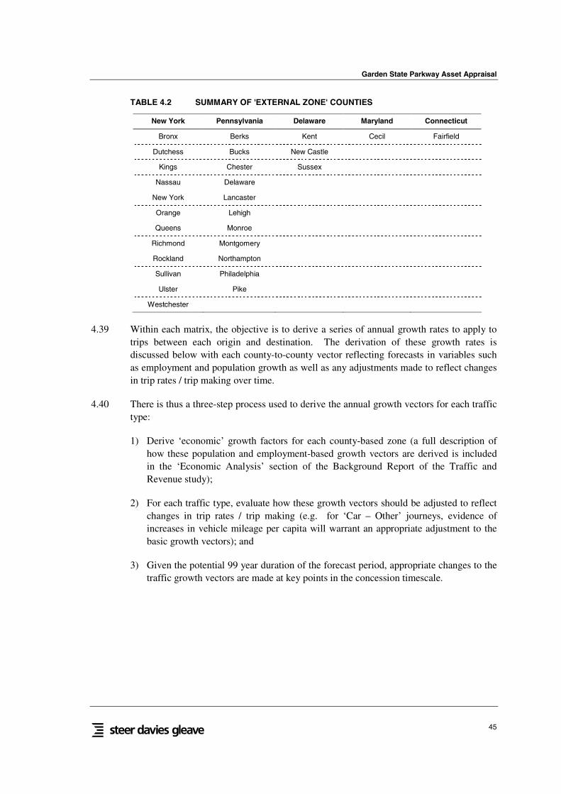
Garden State Parkway Asset Appraisal
45
TABLE 4.2 SUMMARY OF 'EXTERNAL ZONE' COUNTIES
New York Pennsylvania Delaware Maryland Connecticut
Bronx Berks Kent Cecil Fairfield
Dutchess Bucks New Castle
Kings Chester Sussex
Nassau Delaware
New York Lancaster
Orange Lehigh
Queens Monroe
Richmond Montgomery
Rockland Northampton
Sullivan Philadelphia
Ulster Pike
Westchester
4.39 Within each matrix, the objective is to derive a series of annual growth rates to apply totrips between each origin and destination. The derivation of these growth rates isdiscussed below with each county-to-county vector reflecting forecasts in variables suchas employment and population growth as well as any adjustments made to reflect changesin trip rates / trip making over time.
4.40 There is thus a three-step process used to derive the annual growth vectors for each traffictype:
1) Derive ‘economic’ growth factors for each county-based zone (a full description ofhow these population and employment-based growth vectors are derived is includedin the ‘Economic Analysis’ section of the Background Report of the Traffic andRevenue study);
2) For each traffic type, evaluate how these growth vectors should be adjusted to reflectchanges in trip rates / trip making (e.g. for ‘Car – Other’ journeys, evidence ofincreases in vehicle mileage per capita will warrant an appropriate adjustment to thebasic growth vectors); and
3) Given the potential 99 year duration of the forecast period, appropriate changes to thetraffic growth vectors are made at key points in the concession timescale.
Garden State Parkway Asset Appraisal
46
4.41 If appropriate, matrix ‘Furnessing’3 is undertaken for those traffic types where originvectors (e.g. based on ‘population’ growth) are different to destination vectors (e.g. basedon ‘employment’ growth). This technique has been specifically applied to the ‘Car –work’ category where origins are related to population growth and destinations based onemployment forecasts.
4.42 The format of the output from the traffic growth matrices are then converted to the trafficmodel’s zone structure for input to the traffic model.
Car - Work
4.43 For car-based journeys to work, we have used county employment growth vectors as abasis for ‘destination’ trips. This is because growth in this traffic category will be veryclosely linked to growth in at ‘employment destinations’. For the ‘origin’ trips, these arebased on forecast increases in population in each county as the relative growth in thenumber of residents will also influence the rate of increase in work trips.
4.44 Given that there will be differing rates of growth at both origins and destinations withinthe ‘Car – Work’ matrices, these are ‘balanced’ by use of an appropriate ‘Furnessing’process. Through a series of iterations, this ensures that the resulting row totals of tripsmatches the column totals of trips.
4.45 The growth rates in the table are annual vectors applicable to the earlier years of theconcession period. Over time, it is necessary to adjust these vectors as it becomesincreasingly difficult to forecast changes in economic variables over the long term. Theprofile indicated below applies to all growth vectors:
• 2007 – 2025: annual growth vectors are based on those indicated in the table above;
• 2026 – 2050: all growth vectors are reduced by 25%;
• 2051 – 2075: all growth vectors are reduced by 50%; and
• 2076 – 2107: all growth vectors are reduced to zero as there is considerableuncertainty surrounding growth levels so far into the future.
3 Furnessing: Process by which traffic volumes are adjusted using an iterative process in order to satisfy defined controltotals
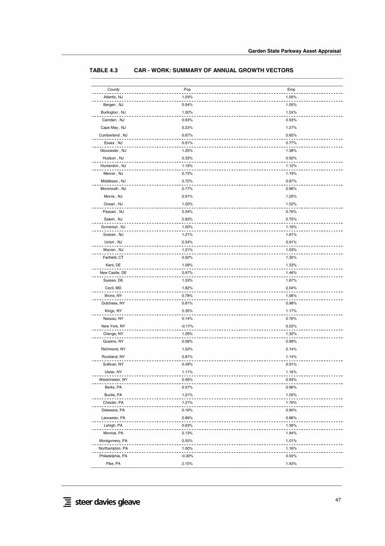
Garden State Parkway Asset Appraisal
47
TABLE 4.3 CAR - WORK: SUMMARY OF ANNUAL GROWTH VECTORS
County Pop Emp
Atlantic, NJ 1.03% 1.00%
Bergen , NJ 0.54% 1.05%
Burlington , NJ 1.00% 1.24%
Camden , NJ 0.63% 0.93%
Cape May , NJ 0.23% 1.27%
Cumberland , NJ 0.67% 0.85%
Essex , NJ 0.51% 0.77%
Gloucester , NJ 1.25% 1.38%
Hudson , NJ 0.33% 0.92%
Hunterdon , NJ 1.19% 1.12%
Mercer , NJ 0.73% 1.19%
Middlesex , NJ 0.72% 0.87%
Monmouth , NJ 0.77% 0.96%
Morris , NJ 0.91% 1.25%
Ocean , NJ 1.20% 1.52%
Passaic , NJ 0.54% 0.76%
Salem , NJ 0.83% 0.75%
Somerset , NJ 1.00% 1.16%
Sussex , NJ 1.21% 1.61%
Union , NJ 0.54% 0.91%
Warren , NJ 1.21% 1.03%
Fairfield, CT 0.52% 1.35%
Kent, DE 1.09% 1.33%
New Castle, DE 0.97% 1.46%
Sussex, DE 1.53% 1.67%
Cecil, MD 1.82% 2.04%
Bronx, NY 0.78% 1.06%
Dutchess, NY 0.81% 0.98%
Kings, NY 0.35% 1.17%
Nassau, NY 0.14% 0.76%
New York, NY -0.17% 0.22%
Orange, NY 1.26% 1.32%
Queens, NY 0.58% 0.99%
Richmond, NY 1.53% 2.14%
Rockland, NY 0.81% 1.14%
Sullivan, NY 0.49% 0.91%
Ulster, NY 1.11% 1.16%
Westchester, NY 0.56% 0.93%
Berks, PA 0.57% 0.96%
Bucks, PA 1.21% 1.55%
Chester, PA 1.21% 1.76%
Delaware, PA 0.19% 0.90%
Lancaster, PA 0.86% 0.86%
Lehigh, PA 0.63% 1.36%
Monroe, PA 2.13% 1.94%
Montgomery, PA 0.55% 1.01%
Northampton, PA 1.00% 1.16%
Philadelphia, PA -0.30% 0.50%
Pike, PA 2.15% 1.93%
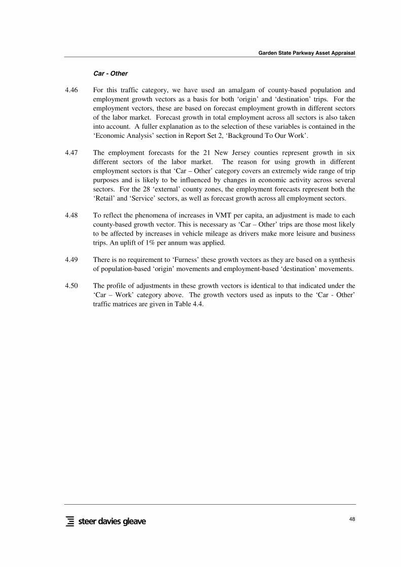
Garden State Parkway Asset Appraisal
48
Car - Other
4.46 For this traffic category, we have used an amalgam of county-based population andemployment growth vectors as a basis for both ‘origin’ and ‘destination’ trips. For theemployment vectors, these are based on forecast employment growth in different sectorsof the labor market. Forecast growth in total employment across all sectors is also takeninto account. A fuller explanation as to the selection of these variables is contained in the‘Economic Analysis’ section in Report Set 2, ‘Background To Our Work’.
4.47 The employment forecasts for the 21 New Jersey counties represent growth in sixdifferent sectors of the labor market. The reason for using growth in differentemployment sectors is that ‘Car – Other’ category covers an extremely wide range of trippurposes and is likely to be influenced by changes in economic activity across severalsectors. For the 28 ‘external’ county zones, the employment forecasts represent both the‘Retail’ and ‘Service’ sectors, as well as forecast growth across all employment sectors.
4.48 To reflect the phenomena of increases in VMT per capita, an adjustment is made to eachcounty-based growth vector. This is necessary as ‘Car – Other’ trips are those most likelyto be affected by increases in vehicle mileage as drivers make more leisure and businesstrips. An uplift of 1% per annum was applied.
4.49 There is no requirement to ‘Furness’ these growth vectors as they are based on a synthesisof population-based ‘origin’ movements and employment-based ‘destination’ movements.
4.50 The profile of adjustments in these growth vectors is identical to that indicated under the‘Car – Work’ category above. The growth vectors used as inputs to the ‘Car - Other’traffic matrices are given in Table 4.4.
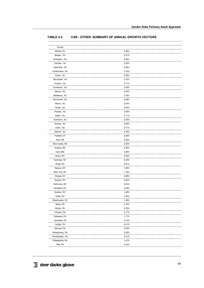
Garden State Parkway Asset Appraisal
49
TABLE 4.4 CAR - OTHER: SUMMARY OF ANNUAL GROWTH VECTORS
County
Atlantic, NJ 2.39%
Bergen , NJ 2.27%
Burlington , NJ 2.56%
Camden , NJ 2.20%
Cape May , NJ 2.36%
Cumberland , NJ 2.16%
Essex , NJ 2.03%
Gloucester , NJ 2.75%
Hudson , NJ 2.11%
Hunterdon , NJ 2.53%
Mercer , NJ 2.44%
Middlesex , NJ 2.19%
Monmouth , NJ 2.28%
Morris , NJ 2.54%
Ocean , NJ 2.84%
Passaic , NJ 2.02%
Salem , NJ 2.11%
Somerset , NJ 2.50%
Sussex , NJ 2.92%
Union , NJ 2.17%
Warren , NJ 2.46%
Fairfield, CT 2.26%
Kent, DE 2.55%
New Castle, DE 2.32%
Sussex, DE 2.93%
Cecil, MD 3.38%
Bronx, NY 2.05%
Dutchess, NY 2.16%
Kings, NY 2.01%
Nassau, NY 1.66%
New York, NY 1.16%
Orange, NY 2.68%
Queens, NY 2.00%
Richmond, NY 3.04%
Rockland, NY 2.28%
Sullivan, NY 1.82%
Ulster, NY 2.32%
Westchester, NY 1.98%
Berks, PA 2.10%
Bucks, PA 2.72%
Chester, PA 2.77%
Delaware, PA 1.71%
Lancaster, PA 2.14%
Lehigh, PA 2.41%
Monroe, PA 3.23%
Montgomery, PA 2.03%
Northampton, PA 2.31%
Philadelphia, PA 1.47%
Pike, PA 3.15%
Garden State Parkway Asset Appraisal
50
Trucks
4.51 For truck traffic, extensive use was made of ‘Trend Analysis’ of past growth as well asforecasts of truck movements made by organizations such as the Federal HighwayAdministration’s (FHWA’s) Freight Analysis Framework (FAF). The latter comprises,for example, forecasts of truck movements by county in New Jersey.
4.52 The findings from this analysis show that truck traffic growth in New Jersey, bothobserved and forecast, is extremely robust with the key findings being:
• Based on data from the NJTA, observed truck traffic on the NJTP over the 15 yearperiod from 1991 to 2006 grew at an average of 2.5% per annum (with slightlynegative growth in the years following the events of 9/11), as shown in Figure 4.7;
• According to data from the Bureau of Transportation Statistics, total truck tonmileage across New Jersey increased by just over 2.6% per annum between 1993 and2002 (over the shorter period between 1997 and 2002, annual growth was just over2.5%); and
• According to the FHWA’s Freight Analysis Framework, forecast annual growth intruck traffic across all 21 New Jersey counties is predicted to be 2.7% per annumbetween 1998 and 2020.
FIGURE 4.7 NJTP - YEAR ON YEAR TRUCK TRAFFIC GROWTH 1992-2005
-4.0%
-2.0%
0.0%
2.0%
4.0%
6.0%
8.0%
1992
1993
1994
1995
1996
1997
1998
1999
2000
2001
2002
2003
2004
2005
Source: NJTA / SDG Analysis
4.53 Although there have been fluctuations in truck traffic across different years, the 15-yearaverage growth of 2.5% per annum is consistent with that observed across the State since1993. In addition, historic growth in the New Jersey’s Gross State Product is very similar,at 2.5% on average between 1998 and 2005.
4.54 There thus appears to be a very close link between historic truck traffic and economicactivity in the State. This is reflected in our selection of truck growth vectors.
Garden State Parkway Asset Appraisal
51
4.55 We have based the selection of truck growth vectors on the basis of these findings andhave derived a growth vector of 2.5% per annum across all county-based zones;
4.56 The selection of a vector of 2.5% appears prudent given both observed truck traffic andGross State Product growth in the State as well as the forecasts for growth in these twoparameters. Woods & Poole, for example, forecast that Gross State Product growth inNew Jersey will be close to 2.5% per annum.
4.57 Similar to the ‘Car – Work’ and ‘Car – Other’ traffic categories, annual truck growth isadjusted by the same profile of adjustments given in Paragraph 4.48.

Garden State Parkway Asset Appraisal
52
5. FORECASTS
Introduction
5.1 Traffic and Revenue forecasts have been developed, for a scenario which has been definedas the most likely outcome, taking into account the balance of probabilities with all thedifferent risks and uncertainties in any forecasting process.
5.2 The revenues presented in the report are in real terms – the price base for the results is2006. Table 5.1 below summarizes the main assumptions underlying the forecasts.
TABLE 5.1 SUMMARY OF FORECASTING ASSUMPTIONS
Item
Base Year Demand andRevenue
2006 Transaction Databases for NJTP / GSP and ACE providingtransactions and revenues by location, day of year, payment type andtoll rate – provided by toll authorities
General assumption on exempted traffic and others: reflected in averagetoll per vehicle taken from Transaction database
O/D Pattern and Journeypurpose split
Taken from State-wide model. Matrices updated with NJTPA andSJTPO (including DVRPC) data.
2 time periods: Peak (represented by AM flow direction) and Off Peak.The factors applied to each period come from most recent NJTPA scriptparameters adjusted using count data available for 24 hours period.
Segmentation by 2 journey purposes (home based work and other), bothjourney purposes split into four income groups. The four income groupsare based on county-level Census 2000 household income levels fit intothe income ranges of the four income groups identified in the NJTPA(values grown to 2000). Number of households in each income groupconverted to trips using the income group trip levels in NJTPAdocumentation.
Commercial vehicles treated as one segment.
Traffic Growth – Cars(work journeys)
Based on economic growth variables for 21 New Jersey counties and 28‘external’ counties
Key parameters are annual 2005 – 2025 employment & population andforecasts (sources: Woods & Poole, DLWFD & Metropolitan PlanningOrganizations)
For ‘origin’ trips, population growth vectors are used and for ‘destination’trips, employment growth vectors are used
Origin-based & destination-based growth is then ‘balanced’ within thematrix by using an appropriate ‘Furnessing’ process
Garden State Parkway Asset Appraisal
53
Traffic Growth – Cars(‘other’ journeys)
Based on economic growth variables for 21 New Jersey counties and 28‘external’ counties
Key parameters are annual 2005 – 2025 population & employmentforecasts – the latter are based on forecasts across a variety of labormarket sectors (sources: Woods & Pool, DLWFD & MetropolitanPlanning Organizations)
The vectors from the different labor markets are then weighted accordingto assumptions about what proportions form ‘total’ growth – thepopulation vectors are also ‘weighted’ as part of this process
Further adjustments to growth factors: for this traffic category, the annualgrowth vectors are multiplied by 1% to reflect observed increased inVehicle Miles Traveled, VMT, per capita.
Traffic Growth - Trucks Based on analysis of historic & forecast truck traffic trends throughoutNew Jersey, truck growth is based on forecast State-wide GDP growth.
Highway Model Network Taken from State-wide model and updated to reflect coding of North andSJTPA networks for significant roads. Also updated to reflect other keycoding elements (e.g. Auto only section of New Jersey Turnpike).
Link speeds and capacities based on NJTPA values.
New Jersey Turnpike free flow speeds are set at 70 mph regardless ofthe area type.
Link volume-delay relationships follow the conventional BPR function(a=0.15, b=4.0) for high-type roadways (tollways, freeways, expresswaysand divided principal arterials), and follow a modified BPR function(a=0.135, b=5.35) for lower-type roadways. The modified BPR functionwas estimated from graphical presentations of the relationships used inthe NJTPA.
All significant toll plazas were coded for two-way collection to avoidcreating unrealistic differences in assigned traffic volumes in the O->Dand D->O directions.
Highway Model NetworkToll Rates
Taken from State-wide model and updated with current NJT, GSP, andACE toll rates, as well as current toll rates of bridge crossings to/from NJto Delaware, New York, and Pennsylvania.
Year of dollar in Modelruns
All model runs include tolls, and values of time in 2006 dollars. VOT areassumed to remain constant in real terms in the future.
Traffic AssignmentPrinciple
Equilibrated generalized cost, where generalized cost is travel timeadjusted for motorway bonus * VOT + travel distance * VOC + toll. Ineach iteration, the equilibration procedure determined a minimumgeneralized cost OD path for each distinct user class, reflecting theclass’s individual VOT and VOC.
Equilibrium CalculationTolerance
An assignment tolerance of 0.05 was used.
Garden State Parkway Asset Appraisal
54
Value of Time (VOT)(2006 prices)
Based on Census 2000 Household income levels. Household incomelevels were converted into average wage rate by dividing by 2080 hours;commuter VOTs were calculated as 50% of the wage rate, and otherVOTs as 35% of the wage rate ($ / hr):
• Car Commute: 4.2 / 10.8 / 18.1 / 36.9
• Car Other: 2.9 / 7.6 / 12.7 / 25.9
Trucks: 54.25
Value of Time Growth Assumed constant in the future
Perceived VehicleOperating Cost (VOC)(2006 prices)
Auto VOC ($/mile):0.01
Truck VOC was calculated as a 2 X multiple of auto VOC.
Motorway Bonus A 30%-35% bonus for time spent traveling on motorways was applied inthe generalized cost calculation. This bonus was computed on a linkbasis, by reducing the travel time by 30-35% for motorway links.
Toll Road Time Savingscompared to other routes
Based on an equilibrium assignment model.
Journey time surveys undertaken for validation purposes.
Tolling Policy Scenarios as defined by New Jersey
E-ZPass Penetration Assumed constant in the future.
Lane Expansions Additional lanes set out in Appendix C.
Toll Scenarios
5.3 For the Phase 2 traffic and revenue forecasts, a number of toll scenarios have been definedby the State, as follows.
• Control Case - 2% annual inflationary increases levied in arrears 1/1/2010, 1/1/2014and every 4th year thereafter. An annual inflationary increase of 2% has beenassumed, as defined by the State. (Scenario I);
• Control Case PLUS 25% real toll increases 1/1/2010, 1/1/2014 and 1/1/2018(Scenario II);
• Control Case PLUS 50% real toll increases 1/1/2010 and 1/1/2014 (Scenario III)
• Control Case PLUS 50% real toll increases 1/1/2010, 1/1/2014 and 1/1/2018(Scenario IV);
• Control Case PLUS 50% real toll increases 1/1/2010, 1/1/2014, 1/1/2018 and1/1/2022 (Scenario V); and
• Control Case PLUS 75% real toll increases 1/1/2010, 1/1/2018 and 50% 1/1/2022 onthe NJTP, ACE and Rte 440 and a 75% real toll increase 1/1/2010 and 50% in 2018on the GSP (Scenario VI).
5.4 The scenarios represent a range of toll policies. Scenario I (SCI) sees tolls kept constantin real terms. Scenario V (SCV) implies toll rates by 2026 that are almost five timeshigher in real terms than they are today.
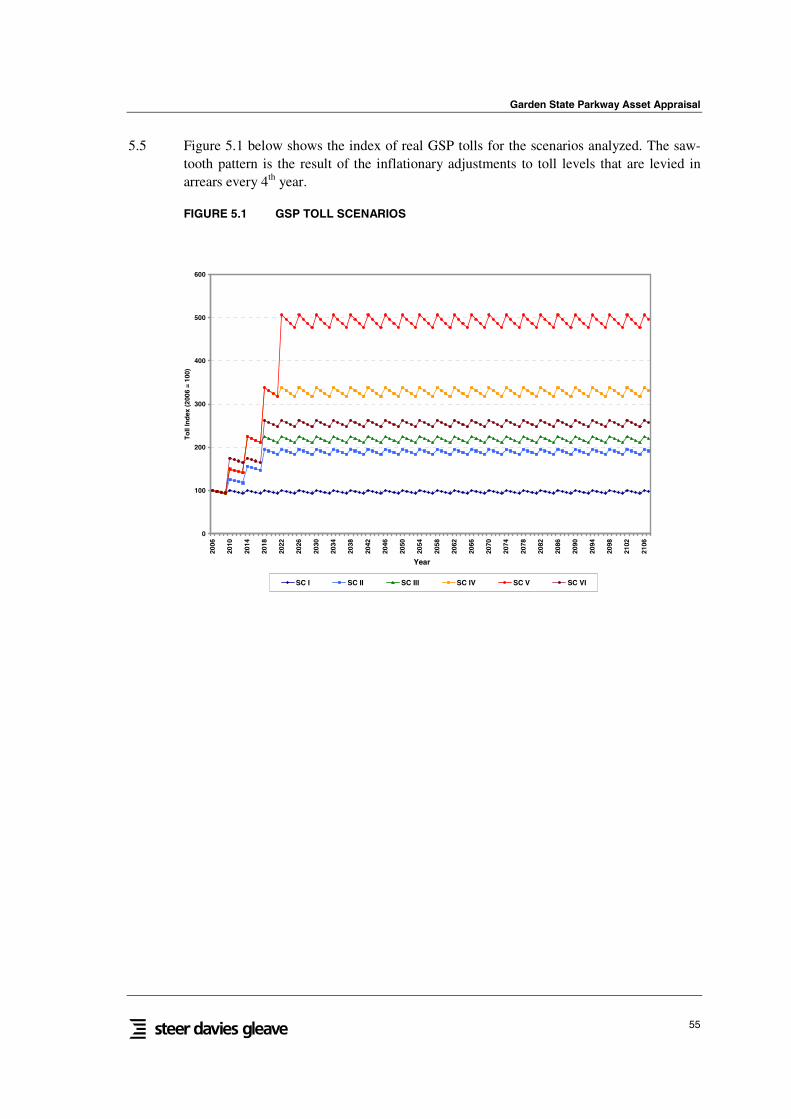
Garden State Parkway Asset Appraisal
55
5.5 Figure 5.1 below shows the index of real GSP tolls for the scenarios analyzed. The saw-tooth pattern is the result of the inflationary adjustments to toll levels that are levied inarrears every 4th year.
FIGURE 5.1 GSP TOLL SCENARIOS
0
100
200
300
400
500
600
2006
2010
2014
2018
2022
2026
2030
2034
2038
2042
2046
2050
2054
2058
2062
2066
2070
2074
2078
2082
2086
2090
2094
2098
2102
2106
Year
To
llIn
dex
(200
6=
100)
SC I SC II SC III SC IV SC V SC VI
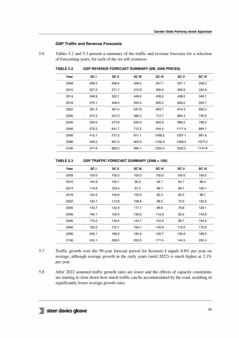
Garden State Parkway Asset Appraisal
56
GSP Traffic and Revenue Forecasts
5.6 Tables 5.2 and 5.3 present a summary of the traffic and revenue forecasts for a selectionof forecasting years, for each of the six toll scenarios.
TABLE 5.2 GSP REVENUE FORECAST SUMMARY ($M, 2006 PRICES)
Year SC I SC II SC III SC IV SC V SC VI
2008 208.5 208.4 208.4 207.1 207.1 208.2
2010 227.5 271.7 310.9 306.9 306.9 332.8
2014 248.8 352.1 449.0 438.0 438.0 348.1
2018 270.1 448.0 493.4 606.2 606.2 550.7
2022 291.4 487.5 537.8 659.7 810.3 692.5
2026 312.5 527.0 582.2 712.7 884.4 740.6
2036 334.5 573.8 635.6 802.9 989.2 798.2
2046 376.2 641.7 712.2 916.4 1117.4 894.1
2066 415.7 727.5 811.1 1048.2 1297.1 991.6
2086 449.2 807.4 903.3 1156.9 1468.4 1077.2
2106 477.6 882.0 990.1 1255.5 1620.2 1147.8
TABLE 5.3 GSP TRAFFIC FORECAST SUMMARY (2008 = 100)
Year SC I SC II SC III SC IV SC V SC VI
2008 100.0 100.0 100.0 100.0 100.0 100.0
2010 104.9 100.1 95.3 94.7 94.7 88.4
2014 114.6 103.4 91.2 89.7 89.7 100.1
2018 124.3 104.8 100.0 82.3 82.3 98.1
2022 134.1 113.8 108.8 89.5 73.0 120.0
2026 143.7 122.9 117.7 96.6 79.6 128.1
2036 160.1 139.3 133.6 112.6 92.2 143.9
2046 173.2 149.5 143.7 122.9 99.7 154.9
2066 192.2 170.1 164.1 140.9 115.6 172.8
2086 209.1 189.9 183.9 156.7 130.8 189.0
2106 224.1 208.5 202.6 171.4 144.5 202.4
5.7 Traffic growth over the 99-year forecast period for Scenario I equals 0.8% per year onaverage, although average growth in the early years (until 2022) is much higher at 2.1%per year.
5.8 After 2022 assumed traffic growth rates are lower and the effects of capacity constraintsare starting to slow down how much traffic can be accommodated by the road, resulting insignificantly lower average growth rates.
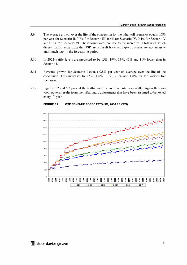
Garden State Parkway Asset Appraisal
57
5.9 The average growth over the life of the concession for the other toll scenarios equals 0.8%per year for Scenario II, 0.7% for Scenario III, 0.6% for Scenario IV, 0.4% for Scenario Vand 0.7% for Scenario VI. These lower rates are due to the increases in toll rates whichdiverts traffic away from the GSP. As a result however capacity issues are not an issueuntil much later in the forecasting period.
5.10 In 2022 traffic levels are predicted to be 15%, 19%, 33%, 46% and 11% lower than inScenario I.
5.11 Revenue growth for Scenario I equals 0.8% per year on average over the life of theconcession. This increases to 1.5%, 1.6%, 1.9%, 2.1% and 1.8% for the various tollscenarios.
5.12 Figures 5.2 and 5.3 present the traffic and revenue forecasts graphically. Again the saw-tooth pattern results from the inflationary adjustments that have been assumed to be leviedevery 4th year.
FIGURE 5.2 GSP REVENUE FORECASTS ($M, 2006 PRICES)
0
200
400
600
800
1,000
1,200
1,400
1,600
1,800
2008
2011
2014
2017
2020
2023
2026
2029
2032
2035
2038
2041
2044
2047
2050
2053
2056
2059
2062
2065
2068
2071
2074
2077
2080
2083
2086
2089
2092
2095
2098
2101
2104
2107
SC I SC II SC III SC IV SC V SC VI
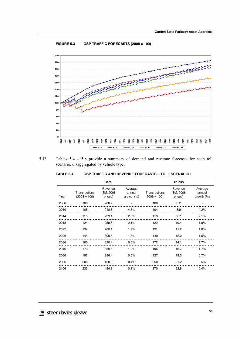
Garden State Parkway Asset Appraisal
58
FIGURE 5.3 GSP TRAFFIC FORECASTS (2008 = 100)
0
20
40
60
80
100
120
140
160
180
200
220
240
2008
2011
2014
2017
2020
2023
2026
2029
2032
2035
2038
2041
2044
2047
2050
2053
2056
2059
2062
2065
2068
2071
2074
2077
2080
2083
2086
2089
2092
2095
2098
2101
2104
2107
SC I SC II SC III SC IV SC V SC VI
5.13 Tables 5.4 – 5.8 provide a summary of demand and revenue forecasts for each tollscenario, disaggregated by vehicle type.
TABLE 5.4 GSP TRAFFIC AND REVENUE FORECASTS – TOLL SCENARIO I
Cars Trucks
YearTrans-actions(2008 = 100)
Revenue($M, 2006
prices)
Averageannual
growth (%)Trans-actions2006 = 100)
Revenue($M, 2006
prices)
Averageannual
growth (%)
2008 100 200.2 - 100 8.2 -
2010 105 218.6 4.5% 104 8.9 4.2%
2014 115 239.1 2.3% 113 9.7 2.1%
2018 124 259.6 2.1% 122 10.4 1.9%
2022 134 280.1 1.9% 131 11.2 1.8%
2026 144 300.5 1.8% 140 12.0 1.6%
2036 160 320.4 0.6% 172 14.1 1.7%
2046 173 359.5 1.2% 196 16.7 1.7%
2066 192 396.4 0.5% 227 19.3 0.7%
2086 208 428.0 0.4% 250 21.2 0.5%
2106 223 454.8 0.3% 270 22.8 0.4%

Garden State Parkway Asset Appraisal
59
TABLE 5.5 GSP TRAFFIC AND REVENUE FORECASTS – TOLL SCENARIO II
Cars Trucks
YearTrans-actions(2008 = 100)
Revenue($M, 2006
prices)
Averageannual
growth (%)Trans-actions2006 = 100)
Revenue($M, 2006
prices)
Averageannual
growth (%)
2008 100 200.2 - 100 8.3 -
2010 100 260.8 14.1% 102 10.9 14.9%
2014 103 337.8 6.7% 107 14.3 7.0%
2018 105 429.5 6.2% 110 18.5 6.7%
2022 114 467.6 2.1% 119 19.9 1.9%
2026 123 505.6 2.0% 127 21.3 1.7%
2036 139 548.6 0.8% 157 25.2 1.7%
2046 149 611.7 1.1% 180 30.0 1.8%
2066 169 692.1 0.6% 213 35.4 0.8%
2086 189 767.6 0.5% 241 39.8 0.6%
2106 208 838.2 0.4% 267 43.8 0.5%
TABLE 5.6 GSP TRAFFIC AND REVENUE FORECASTS – TOLL SCENARIO III
Cars Trucks
YearTrans-actions(2008 = 100)
Revenue($M, 2006
prices)
Averageannual
growth (%)Trans-actions2006 = 100)
Revenue($M, 2006
prices)
Averageannual
growth (%)
2008 100 200.2 - 100 8.3 -
2010 95 298.2 22.1% 99 12.7 24.1%
2014 91 430.2 9.6% 98 18.8 10.3%
2018 100 473.1 2.4% 105 20.3 1.9%
2022 109 516.1 2.2% 113 21.7 1.7%
2026 118 559.1 2.0% 120 23.2 1.6%
2036 133 607.8 0.8% 150 27.8 1.8%
2046 143 679.3 1.1% 171 32.9 1.7%
2066 163 772.0 0.6% 204 39.1 0.9%
2086 183 858.8 0.5% 234 44.4 0.6%
2106 202 940.8 0.5% 260 49.3 0.5%
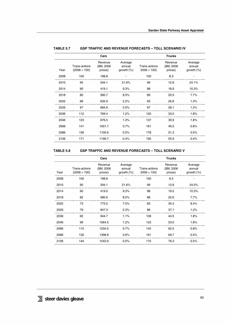
Garden State Parkway Asset Appraisal
60
TABLE 5.7 GSP TRAFFIC AND REVENUE FORECASTS – TOLL SCENARIO IV
Cars Trucks
YearTrans-actions(2008 = 100)
Revenue($M, 2006
prices)
Averageannual
growth (%)Trans-actions2006 = 100)
Revenue($M, 2006
prices)
Averageannual
growth (%)
2008 100 198.8 - 100 8.3 -
2010 95 294.1 21.6% 99 12.8 24.1%
2014 90 419.1 9.3% 98 18.9 10.3%
2018 82 580.7 8.5% 89 25.5 7.7%
2022 89 632.9 2.2% 93 26.8 1.3%
2026 97 684.6 2.0% 97 28.1 1.2%
2036 112 769.4 1.2% 120 33.5 1.8%
2046 123 876.5 1.3% 137 39.9 1.8%
2066 141 1001.7 0.7% 161 46.5 0.8%
2086 156 1105.6 0.5% 178 51.3 0.5%
2106 171 1199.7 0.4% 195 55.9 0.4%
TABLE 5.8 GSP TRAFFIC AND REVENUE FORECASTS – TOLL SCENARIO V
Cars Trucks
YearTrans-actions(2008 = 100)
Revenue($M, 2006
prices)
Averageannual
growth (%)Trans-actions2006 = 100)
Revenue($M, 2006
prices)
Averageannual
growth (%)
2008 100 198.8 - 100 8.3 -
2010 95 294.1 21.6% 99 12.8 24.0%
2014 90 419.0 9.3% 98 19.0 10.3%
2018 82 580.6 8.5% 88 25.6 7.7%
2022 73 775.0 7.5% 83 35.4 8.4%
2026 79 847.3 2.3% 86 37.1 1.2%
2036 92 944.7 1.1% 108 44.5 1.8%
2046 99 1064.5 1.2% 123 53.0 1.8%
2066 115 1234.5 0.7% 145 62.5 0.8%
2086 130 1398.8 0.6% 161 69.7 0.5%
2106 144 1543.9 0.5% 175 76.3 0.5%

Garden State Parkway Asset Appraisal
61
TABLE 5.9 GSP TRAFFIC AND REVENUE FORECASTS – TOLL SCENARIO VI
Cars Trucks
YearTrans-actions(2008 = 100)
Revenue($M, 2006
prices)
Averageannual
growth (%)Trans-actions2006 = 100)
Revenue($M, 2006
prices)
Averageannual
growth (%)
2008 100 200.0 - 100 8.2 -
2010 88 319.5 26.4% 92 13.3 27.6%
2014 100 334.6 1.2% 99 13.5 0.5%
2018 98 528.8 12.1% 98 21.9 12.9%
2022 119 658.3 5.6% 120 26.3 4.7%
2026 127 701.7 1.6% 127 27.9 1.5%
2036 141 748.1 0.6% 152 32.1 1.4%
2046 152 835.7 1.1% 173 37.8 1.7%
2066 169 924.4 0.5% 196 42.9 0.6%
2086 184 1004.0 0.4% 212 46.6 0.4%
2106 197 1068.1 0.3% 225 49.6 0.3%
Garden State Parkway Asset Appraisal
62
Review of Responses in Demand to Toll Changes
5.14 As part of our work we undertook a review of existing studies of how the level of demandfor a toll road might change in the face of changes in toll levels. We note that, in theliterature as elsewhere, this is commonly referred to as a toll elasticity – with aconcomitant perception that such an elasticity revealed on a particular project is in someway general and thus can be transferred/ compared across different projects. This is, ofcourse, not the case: the response of toll road users to changes in toll levels is projectspecific, reflecting the comparative attractions of the toll road and its competitors.However, given that many projects have been constructed in congested areas, withbroadly similar comparative advantage for the tolled facility, it does remain interesting toexamine what has happened on other facilities across the United States.
5.15 It was found that there is a considerable body of existing evidence on so-called demandelasticities, with several studies specific to New Jersey and others relating to other States.
5.16 The tolls on the New Jersey toll roads (NJTP, GSP and ACE) are currently low – incomparison with most other facilities within the United States, and certainly with tolledfacilities in other advanced economies – while the advantage in using the toll road is high.For most users, the level of toll is well below the indifference price: the toll can, for theseusers, be raised very significantly before they will seriously consider using a freealternative. At this point, we would expect the revealed demand elasticity to be very low.However, if the tolls increase significantly the changes in behavior might themselvesbecome measurable, until a new equilibrium is achieved.
5.17 There are recent studies available for the NJTP and for the crossings between New Jerseyand New York, but not for the ACE or the GSP. The evidence from the recent research onthe NJTP Time of Day Pricing Initiative suggests that the demand for the road is relativelyinelastic to price. This is consistent with the available evidence from time-series data oftraffic and revenue for the NJTP, GSP and ACE, which again points to the demand beingrelatively inelastic.
5.18 In the first phase of this study (the Scoping Study), our analysis was based on an elasticityapproach – relying on imported values derived from our experience elsewhere. Elasticityestimates of -0.1 for the NJTP, -0.07 for the GSP and -0.12 for the ACE were adopted,taking on board additional local evidence from time series of transaction and revenue forthe NJTP, the GSP and the ACE. In the Phase 2 analysis, however, we employed theState-wide network assignment model to estimate directly the impact of toll increases onGSP usage; this analysis indicated elasticity estimates in a range from -0.1 to -0.2. Wehave further reviewed the elasticity estimates by time of day, journey purpose and vehicletype. We have found that the out-turn weekday peak elasticities are indeed in line with ourPhase I assumptions, but that off-peak elasticities are significantly higher than thoseadopted earlier. The results obtained from the models are, on review, unsurprising. Theassignment models show traffic diverting onto the competing routes, when (as in the off-peak) capacity is genuinely available.
Garden State Parkway Asset Appraisal
63
5.19 To provide further validation of our results, we reviewed modeled elasticities developed inwork carried out in the development of forecasts for the Indiana Toll Road. On the first 24miles - close to Chicago with high volumes on the road and in the corridor in general -there is a single toll barrier with a toll of c2.08/ mi and c7.29/ mi,. Here the elasticitiesderived from the models were -0.23 (cars) and -0.07 (trucks). In the rest of the 125 milesof the road, which runs across the rural areas in the north of Indiana and is lightly used,the elasticities derived from the models were substantially higher, in the range -0.69 to -0.34 for cars and -0.19 to -0.14 for trucks.
5.20 Similarly, work carried out by Maunsell Aecom on the Houston toll road system lookingat the response of demand to actual toll increases in 2004, suggested effective elasticitiesranging between -0.08 and -0.32. Further, the work showed that, on the predominantlyradial toll roads, the traffic levels were more responsive to toll changes – while the orbitalroutes revealed lower elasticities.
5.21 The 2003 paper "Demand Elasticity on Tolled Motorways" by Anna Matas and José-LuisRaymond for the Journal of Transportation and Statistics states that most demandelasticities are within the -0.2 to -0.3 range, though an overall range of -0.03 to -0.5 wasfound.
5.22 We concluded from this review that the elasticities we derived from the models developedfor the analysis in New Jersey were both realistic in terms of the network performanceacross the State and broadly in line with the behavior of travelers elsewhere.
Garden State Parkway Asset Appraisal
Appendix
APPENDIX A
MAPS
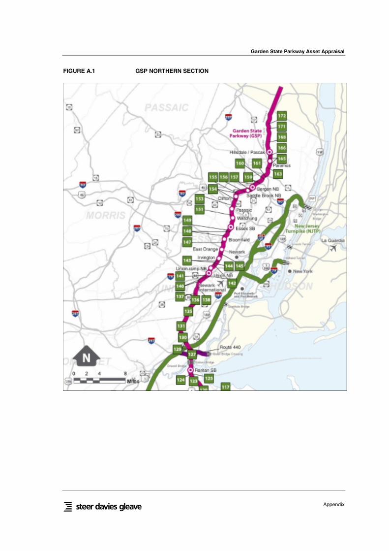
Garden State Parkway Asset Appraisal
Appendix
FIGURE A.1 GSP NORTHERN SECTION
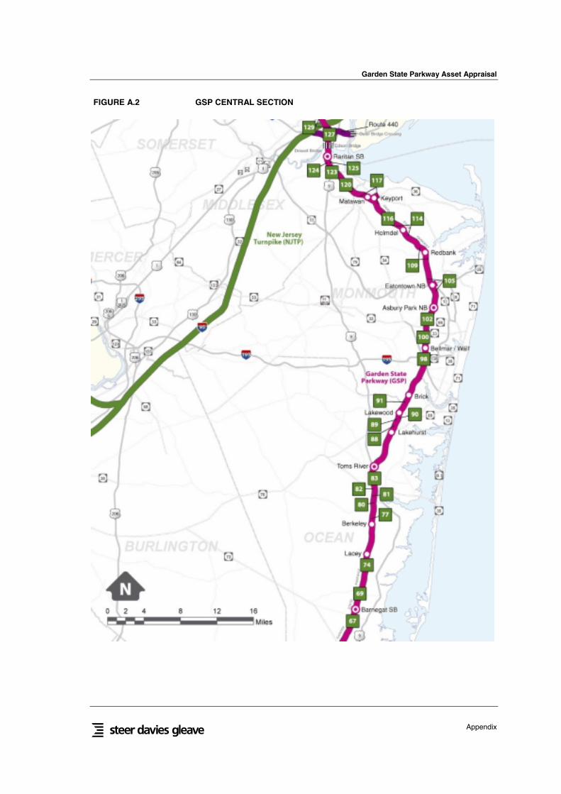
Garden State Parkway Asset Appraisal
Appendix
FIGURE A.2 GSP CENTRAL SECTION

Garden State Parkway Asset Appraisal
Appendix
FIGURE A.3 GSP SOUTHERN SECTION

Garden State Parkway Asset Appraisal
Appendix
APPENDIX B
FORECASTS

Garden State Parkway Asset Appraisal
Appendix
APPENDIX: TABLE B.1 GSP - REVENUE FORECAST SUMMARY ($M, 2006 PRICES)
Year SC I SC II SC III SC IV SC V SC VI
2008 208.5 208.4 208.4 207.1 207.1 208.2
2009 209.4 209.3 209.3 207.3 207.4 209.0
2010 227.5 271.7 310.9 306.9 306.9 332.8
2011 228.3 274.0 314.1 309.2 309.2 337.1
2012 228.9 276.1 317.1 311.3 311.3 341.1
2013 229.4 278.0 319.9 313.2 313.2 344.7
2014 248.8 352.1 449.0 438.0 438.0 348.1
2015 249.1 355.0 454.1 441.9 441.9 351.3
2016 249.4 357.7 458.9 445.5 445.5 354.2
2017 249.5 360.1 463.3 448.8 448.7 356.7
2018 270.1 448.0 493.4 606.2 606.2 550.7
2019 270.0 452.0 497.8 612.5 612.4 553.0
2020 269.8 455.7 501.9 618.2 618.2 555.2
2021 269.6 459.0 505.6 623.5 623.4 557.1
2022 291.4 487.5 537.8 659.7 810.3 692.5
2023 290.8 490.8 541.5 665.1 816.4 693.2
2024 290.2 493.8 544.9 670.0 828.2 693.7
2025 289.5 496.4 547.9 674.1 839.2 693.9
2026 312.5 527.0 582.2 712.7 884.4 740.6
2027 311.1 528.7 584.2 717.1 888.2 739.9
2028 309.3 529.0 584.7 721.7 896.7 738.1
2029 307.4 529.0 584.9 725.8 904.5 735.9
2030 330.5 559.2 618.8 768.1 950.7 783.2
2031 326.9 556.6 616.0 767.6 946.8 777.4
2032 323.3 553.9 613.0 766.8 949.0 771.5
2033 319.7 550.9 609.9 765.8 950.1 765.5
2034 342.1 579.9 642.2 805.4 993.4 811.0
2035 338.3 576.9 639.0 804.3 988.1 804.6
2036 334.5 573.8 635.6 802.9 989.2 798.2
2037 330.7 570.5 632.1 801.3 989.7 791.7
2038 353.7 600.5 665.5 842.6 1035.0 838.7
2039 349.7 597.1 661.9 840.9 1028.9 831.9
2040 345.6 593.6 658.1 838.9 1029.3 825.0
2041 341.6 590.0 654.2 836.5 1029.1 817.9
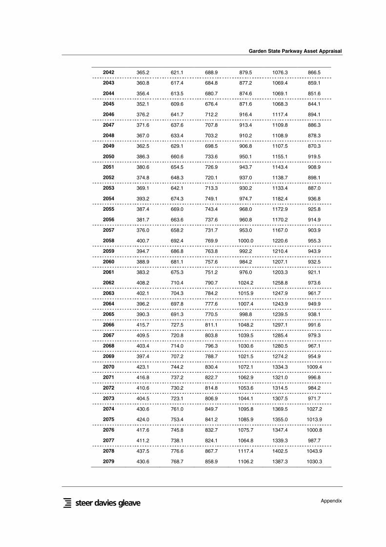
Garden State Parkway Asset Appraisal
Appendix
2042 365.2 621.1 688.9 879.5 1076.3 866.5
2043 360.8 617.4 684.8 877.2 1069.4 859.1
2044 356.4 613.5 680.7 874.6 1069.1 851.6
2045 352.1 609.6 676.4 871.6 1068.3 844.1
2046 376.2 641.7 712.2 916.4 1117.4 894.1
2047 371.6 637.6 707.8 913.4 1109.8 886.3
2048 367.0 633.4 703.2 910.2 1108.9 878.3
2049 362.5 629.1 698.5 906.8 1107.5 870.3
2050 386.3 660.6 733.6 950.1 1155.1 919.5
2051 380.6 654.5 726.9 943.7 1143.4 908.9
2052 374.8 648.3 720.1 937.0 1138.7 898.1
2053 369.1 642.1 713.3 930.2 1133.4 887.0
2054 393.2 674.3 749.1 974.7 1182.4 936.8
2055 387.4 669.0 743.4 968.0 1172.9 925.8
2056 381.7 663.6 737.6 960.8 1170.2 914.9
2057 376.0 658.2 731.7 953.0 1167.0 903.9
2058 400.7 692.4 769.9 1000.0 1220.6 955.3
2059 394.7 686.8 763.8 992.2 1210.4 943.9
2060 388.9 681.1 757.6 984.2 1207.1 932.5
2061 383.2 675.3 751.2 976.0 1203.3 921.1
2062 408.2 710.4 790.7 1024.2 1258.8 973.6
2063 402.1 704.3 784.2 1015.9 1247.9 961.7
2064 396.2 697.8 777.6 1007.4 1243.9 949.9
2065 390.3 691.3 770.5 998.8 1239.5 938.1
2066 415.7 727.5 811.1 1048.2 1297.1 991.6
2067 409.5 720.8 803.8 1039.5 1285.4 979.3
2068 403.4 714.0 796.3 1030.6 1280.5 967.1
2069 397.4 707.2 788.7 1021.5 1274.2 954.9
2070 423.1 744.2 830.4 1072.1 1334.3 1009.4
2071 416.8 737.2 822.7 1062.9 1321.0 996.8
2072 410.6 730.2 814.8 1053.6 1314.5 984.2
2073 404.5 723.1 806.9 1044.1 1307.5 971.7
2074 430.6 761.0 849.7 1095.8 1369.5 1027.2
2075 424.0 753.4 841.2 1085.9 1355.0 1013.9
2076 417.6 745.8 832.7 1075.7 1347.4 1000.8
2077 411.2 738.1 824.1 1064.8 1339.3 987.7
2078 437.5 776.6 867.7 1117.4 1402.5 1043.9
2079 430.6 768.7 858.9 1106.2 1387.3 1030.3
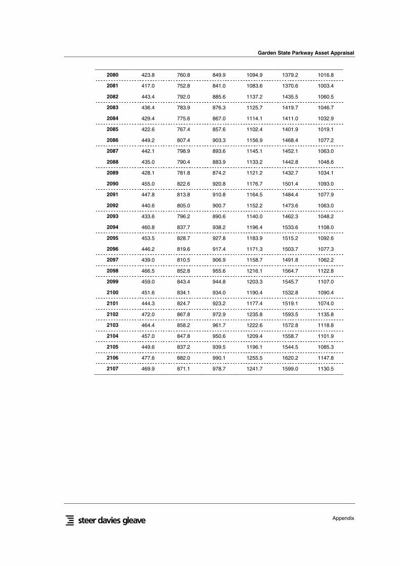
Garden State Parkway Asset Appraisal
Appendix
2080 423.8 760.8 849.9 1094.9 1379.2 1016.8
2081 417.0 752.8 841.0 1083.6 1370.6 1003.4
2082 443.4 792.0 885.6 1137.2 1435.5 1060.5
2083 436.4 783.9 876.3 1125.7 1419.7 1046.7
2084 429.4 775.6 867.0 1114.1 1411.0 1032.9
2085 422.6 767.4 857.6 1102.4 1401.9 1019.1
2086 449.2 807.4 903.3 1156.9 1468.4 1077.2
2087 442.1 798.9 893.6 1145.1 1452.1 1063.0
2088 435.0 790.4 883.9 1133.2 1442.8 1048.6
2089 428.1 781.8 874.2 1121.2 1432.7 1034.1
2090 455.0 822.6 920.8 1176.7 1501.4 1093.0
2091 447.8 813.8 910.8 1164.5 1484.4 1077.9
2092 440.6 805.0 900.7 1152.2 1473.6 1063.0
2093 433.6 796.2 890.6 1140.0 1462.3 1048.2
2094 460.8 837.7 938.2 1196.4 1533.6 1108.0
2095 453.5 828.7 927.8 1183.9 1515.2 1092.6
2096 446.2 819.6 917.4 1171.3 1503.7 1077.3
2097 439.0 810.5 906.9 1158.7 1491.8 1062.2
2098 466.5 852.8 955.6 1216.1 1564.7 1122.8
2099 459.0 843.4 944.8 1203.3 1545.7 1107.0
2100 451.6 834.1 934.0 1190.4 1532.8 1090.4
2101 444.3 824.7 923.2 1177.4 1519.1 1074.0
2102 472.0 867.8 972.9 1235.8 1593.5 1135.8
2103 464.4 858.2 961.7 1222.6 1572.8 1118.8
2104 457.0 847.8 950.6 1209.4 1558.7 1101.9
2105 449.6 837.2 939.5 1196.1 1544.5 1085.3
2106 477.6 882.0 990.1 1255.5 1620.2 1147.8
2107 469.9 871.1 978.7 1241.7 1599.0 1130.5

Garden State Parkway Asset Appraisal
Appendix
APPENDIX C
LANE EXPANSIONS
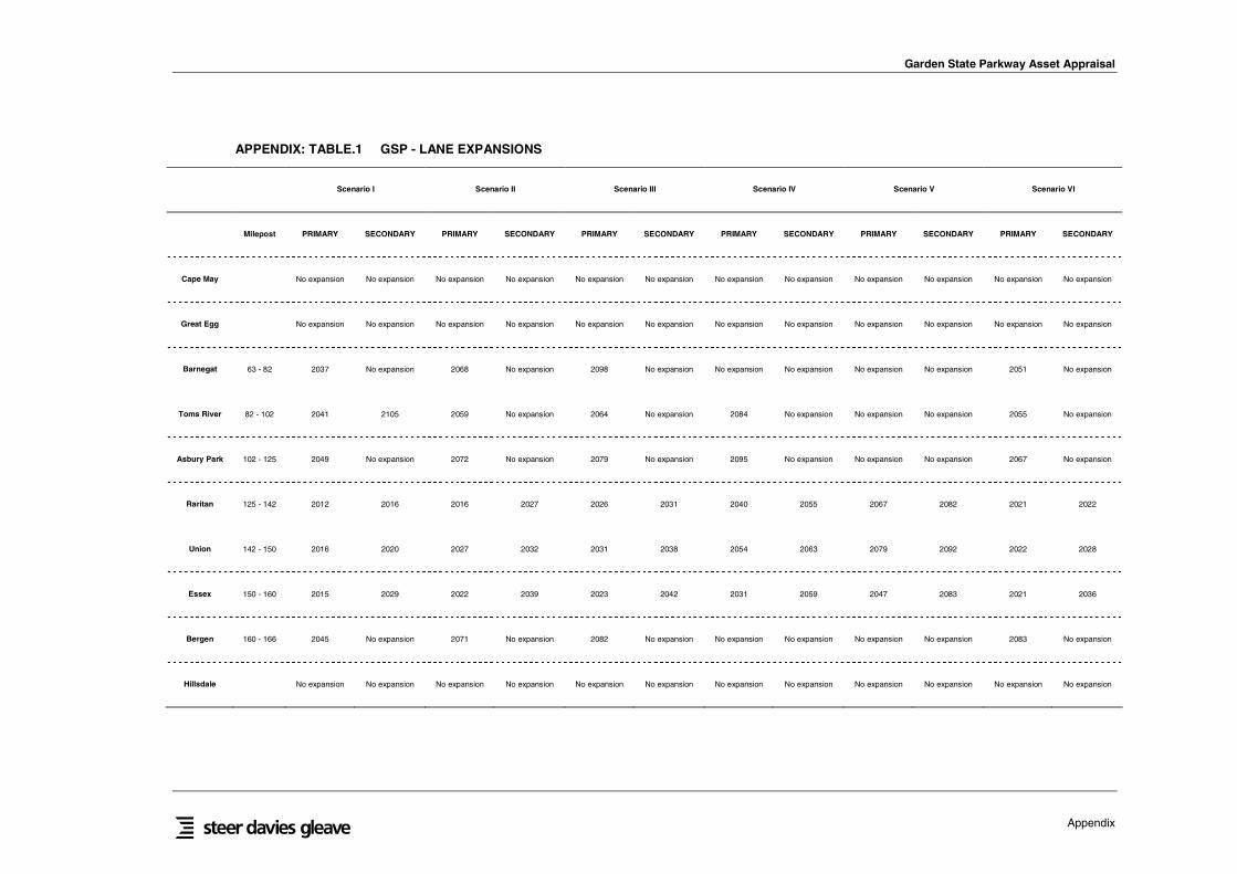
Garden State Parkway Asset Appraisal
Appendix
APPENDIX: TABLE.1 GSP - LANE EXPANSIONS
Scenario I Scenario II Scenario III Scenario IV Scenario V Scenario VI
Milepost PRIMARY SECONDARY PRIMARY SECONDARY PRIMARY SECONDARY PRIMARY SECONDARY PRIMARY SECONDARY PRIMARY SECONDARY
Cape May No expansion No expansion No expansion No expansion No expansion No expansion No expansion No expansion No expansion No expansion No expansion No expansion
Great Egg No expansion No expansion No expansion No expansion No expansion No expansion No expansion No expansion No expansion No expansion No expansion No expansion
Barnegat 63 - 82 2037 No expansion 2068 No expansion 2098 No expansion No expansion No expansion No expansion No expansion 2051 No expansion
Toms River 82 - 102 2041 2105 2059 No expansion 2064 No expansion 2084 No expansion No expansion No expansion 2055 No expansion
Asbury Park 102 - 125 2049 No expansion 2072 No expansion 2079 No expansion 2095 No expansion No expansion No expansion 2067 No expansion
Raritan 125 - 142 2012 2016 2016 2027 2026 2031 2040 2055 2067 2082 2021 2022
Union 142 - 150 2016 2020 2027 2032 2031 2038 2054 2063 2079 2092 2022 2028
Essex 150 - 160 2015 2029 2022 2039 2023 2042 2031 2059 2047 2083 2021 2036
Bergen 160 - 166 2045 No expansion 2071 No expansion 2082 No expansion No expansion No expansion No expansion No expansion 2083 No expansion
Hillsdale No expansion No expansion No expansion No expansion No expansion No expansion No expansion No expansion No expansion No expansion No expansion No expansion