New Algorithms for Fast Discovery ofAssociation Rules �Mohammed Javeed Zaki, Srinivasan Parthasarathy,Mitsunori Ogihara, and Wei LiComputer Science DepartmentUniversity of Rochester, Rochester NY 14627fzaki,srini,ogihara,lig@cs.rochester.eduThe University of RochesterComputer Science DepartmentRochester, New York 14627Technical Report 651July 1997AbstractAssociation rule discovery has emerged as an important problem in knowledgediscovery and data mining. The association mining task consists of identify-ing the frequent itemsets, and then forming conditional implication rules amongthem. In this paper we present e�cient algorithms for the discovery of frequentitemsets, which forms the compute intensive phase of the task. The algorithmsutilize the structural properties of frequent itemsets to facilitate fast discovery.The related database items are grouped together into clusters representing thepotential maximal frequent itemsets in the database. Each cluster induces asub-lattice of the itemset lattice. E�cient lattice traversal techniques are pre-sented, which quickly identify all the true maximal frequent itemsets, and alltheir subsets if desired. We also present the e�ect of using di�erent databaselayout schemes combined with the proposed clustering and traversal techniques.The proposed algorithms scan a (pre-processed) database only once, addressingthe open question in association mining, whether all the rules can be e�cientlyextracted in a single database pass. We experimentally compare the new algo-rithms against the previous approaches, obtaining improvements of more thanan order of magnitude for our test databases.The University of Rochester Computer Science Department supported this work.�This work was supported in part by an NSF Research Initiation Award (CCR-9409120) and ARPAcontract (F19628-94-C-0057).

1 IntroductionKnowledge discovery and data mining (KDD) is an emerging �eld, whose goal is to makesense out of large amounts of collected data, by discovering hitherto unknown patterns. Oneof the central KDD tasks is the discovery of association rules [1]. The prototypical applicationis the analysis of supermarket sales or basket data [2, 5, 3]. Basket data consists of itemsbought by a customer along with the transaction date, time, price, etc. The associationrule discovery task identi�es the group of items most often purchased along with anothergroup of items. For example, we may obtain a rule of the form \80% of customers whobuy bread and milk, also buy butter and eggs at the same time". Besides the retail salesexample, association rules have been useful in predicting patterns in university enrollment,occurrences of words in text documents, census data, and so on.The task of mining association rules over basket data was �rst introduced in [2], whichcan be formally stated as follows: Let I = fi1; i2; � � � ; img be the set of database items.Each transaction, T , in the database, D, has a unique identi�er, and contains a set ofitems, called an itemset. An itemset with k items is called a k-itemset. A subset of kelements is called a k-subset. The support of an itemset is the percentage of transactions inD that contain the itemset. An association rule is a conditional implication among itemsets,A ) B, where itemsets A;B � I, and A \ B = ;. The con�dence of the association rule,given as support(A[B)=support(A), is simply the conditional probability that a transactioncontains B, given that it contains A. The data mining task for association rules can bebroken into two steps. The �rst step consists of �nding all frequent itemsets, i.e., itemsetsthat occur in the database with a certain user-speci�ed frequency, called minimum support.The second step consists of forming the rules among the frequent itemsets. The problem ofidentifying all frequent itemsets is the computationally intensive step in the algorithm. Givenm items, there are potentially 2m frequent itemsets, which form a lattice of subsets over I.However, only a small fraction of the whole lattice space is frequent. This paper presentse�cient methods to discover these frequent itemsets. The rule discovery step is relativelyeasy [3]. Once the support of frequent itemsets is known, rules of the form X � Y ) Y(where Y � X), are generated for all frequent itemsets X, provided the rules meet a desiredcon�dence. Although this step is easy, there remain important research issues in presenting\interesting" rules from the large set of generated rules. If the important issue in the �rststep is that of \quantity" or performance, due to its compute intensive nature, the dominantconcern in the second step is that of \quality" of rules that are generated. See [26, 18]for some approaches to this problem. In this paper we only consider the frequent itemsetsdiscovery step.Related Work Several algorithms for mining associations have been proposed in theliterature [2, 21, 5, 16, 23, 17, 27, 3, 31]. Almost all the algorithms use the downward closureproperty of itemset support to prune the itemset lattice { the property that all subsetsof a frequent itemset must themselves be frequent. Thus only the frequent k-itemsets areused to construct candidate or potential frequent (k + 1)-itemsets. A pass over the databaseis made at each level to �nd the frequent itemsets. The algorithms di�er to the extentthat they prune the search space using e�cient candidate generation procedure. The �rstalgorithm AIS [2] generates candidates on-the- y. All frequent itemsets from the previous1

transaction that are contained in the new transaction are extended with other items in thattransaction. This results in to many unnecessary candidates. The Apriori algorithm [21, 5, 3]which uses a better candidate generation procedure was shown to be superior to earlierapproaches [2, 17, 16]. The DHP algorithm [23] collects approximate support of candidatesin the previous pass for further pruning, however, this optimization may be detrimental toperformance [4]. All these algorithms make multiple passes over the database, once for eachiteration k. The Partition algorithm [27] minimizes I/O by scanning the database only twice.It partitions the database into small chunks which can be handled in memory. In the �rstpass it generates the set of all potentially frequent itemsets (any itemset locally frequent in apartition), and in the second pass their global support is obtained. Another way to minimizethe I/O overhead is to work with only a small sample of the database. An analysis of thee�ectiveness of sampling for association mining was presented in [34], and [31] presents anexact algorithm that �nds all rules using sampling. The recently proposed DIC algorithm[9] dynamically counts candidates of varying length as the database scan progresses, andthus is able to reduce the number of scans. Approaches using only general-purpose DBMSsystems and relational algebra operations have been studied [16, 17], but these don't comparefavorably with the specialized approaches. A number of parallel algorithms have also beenproposed [24, 4, 32, 11, 14, 33].All the above solutions are applicable to only binary data, i.e., either an item is presentin a transaction or it isn't. Other extensions of association rules include mining over datawhere the quantity of items is also considered [28], or mining for rules in the presence ofa taxonomy on items [6, 15]. There has also been work in �nding frequent sequences ofitemsets over temporal data [6, 22, 29, 20].1.1 ContributionThe main limitation of almost all proposed algorithms [2, 5, 21, 23, 3] is that they makerepeated passes over the disk-resident database partition, incurring high I/O overheads.Moreover, these algorithms use complicated hash structures which entails additional overheadin maintaining and searching them, and they typically su�er from poor cache locality [25].The problem with Partition, even though it makes only two scans, is that, as the number ofpartitions is increased, the number of locally frequent itemsets increases. While this can bereduced by randomizing the partition selection, results from sampling experiments [34, 31]indicate that randomized partitions will have a large number of frequent itemsets in common.Partition can thus spend a lot of time in performing redundant computation.Our work contrasts to these approaches in several ways. We present new algorithms forfast discovery of association rules based on our ideas in [33, 35]. The proposed algorithmsscan the pre-processed database exactly once greatly reducing I/O costs. The new algorithmsare characterized in terms of the clustering information used to group related itemsets, andin terms of the lattice traversal schemes used to search for frequent itemsets. We propose twoclustering schemes based on equivalence classes and maximal uniform hypergraph cliques,and we utilize three lattice traversal schemes, based on bottom-up, top-down, and hybridtop-down/bottom-up search. We also present the e�ect of using di�erent database layouts2

{ the horizontal and vertical formats. The algorithms using the vertical format use simpleintersection operations, making them an attractive option for direct implementation on gen-eral purpose database systems. Extensive experimental results are presented contrasting thenew algorithms with previous approaches, with gains of over an order of magnitude usingthe proposed techniques.The rest of the paper is organized as follows. Section 2 provides details of the itemsetclustering techniques, while section 3 describes the lattice traversal techniques. Section 4gives a brief overview of the KDD process and the data layout alternatives. The Apriori,Partitin and six new algorithms employing the above techniques are described in section 5.Our experimental study is presented in in section 6, and our conclusions in section 7.2 Itemset Clustering123 124 125 134 135 145 234 235 245 345

12345

1234 1235 1245 1345 2345

1 2 3 4 5

12 13 14 15 23 24 3525 34 45

Lattice of Subsets of {1,2,3,4,5}

Border ofFrequent Itemsets

1 2 3 4 3 4 5

35 4534

345

12 13 14 23 24 34

234123 134124

1234

Lattice of Subsets of {1,2,3,4}

Lattice of Subsets of {3,4,5}

Sublattices Induced by Maximal Itemsets

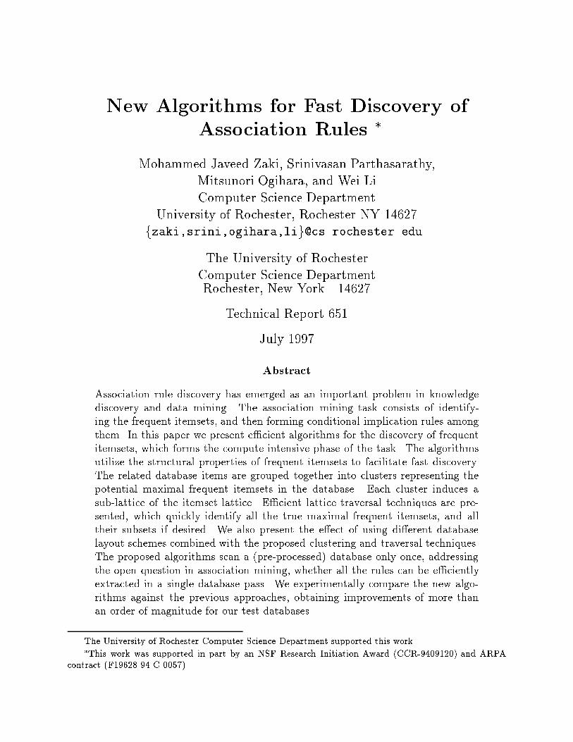
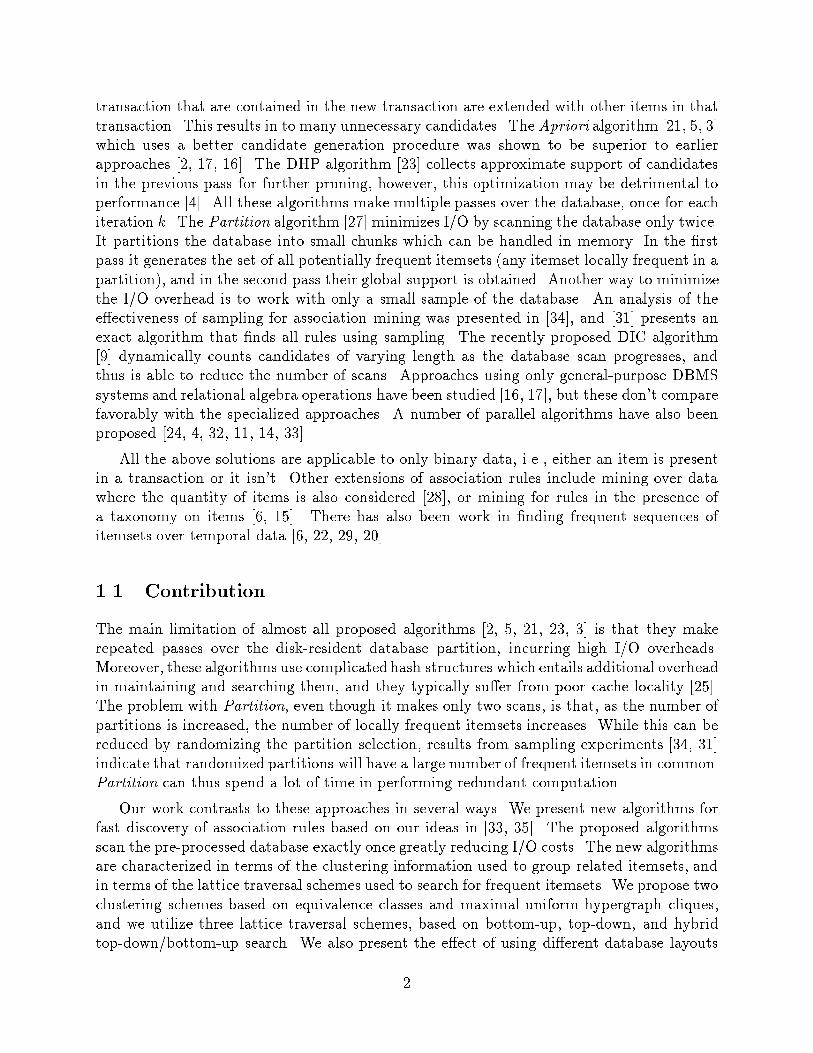
Figure 1: Lattice of Subsets and Maximal Itemset Induced Sub-latticesWe will motivate the need for itemset clustering by means of an example. Consider thelattice of subsets of the set f1; 2; 3; 4; 5g, shown in �gure 1 (the empty set has been omittedin all �gures). The frequent itemsets are shown with dashed circles and the two maximalfrequent itemsets (a frequent itemset is maximal if it is not a proper subset of any otherfrequent itemset) are shown with the bold circles. Due to the downward closure propertyof itemset support { the fact that all subsets of a frequent itemset must be frequent { thefrequent itemsets form a border, such that all frequent itemsets lie below the border, while allinfrequent itemsets lie above it. The border of frequent itemsets is shown with a bold line in�gure 1. An optimal association mining algorithm will only enumerate and test the frequentitemsets, i.e., the algorithm must e�ciently determine the structure of the border. Thisstructure is precisely determined by the maximal frequent itemsets. The border corresponds3

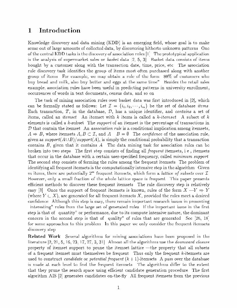
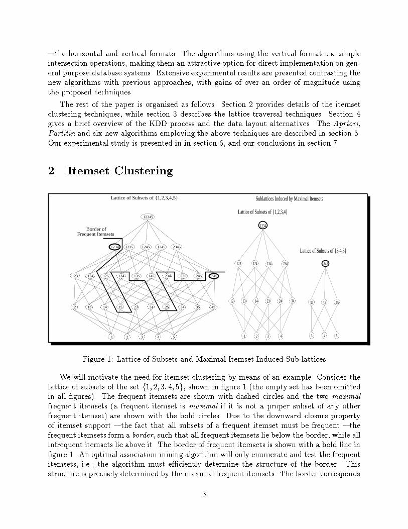
to the sub-lattices induced by the maximal frequent itemsets. These sub-lattices are shownin �gure 1.Given the knowledge of the maximal frequent itemsets we can design an e�cient algo-rithm that simply gathers their support and the support of all their subsets in just a singledatabase pass. In general we cannot precisely determine the maximal itemsets in the inter-mediate steps of the algorithm. However we can approximate this set. Our itemset clusteringtechniques are designed to group items together so that we obtain supersets of the maximalfrequent itemsets { the potential maximal frequent itemsets. Below we present two schemesto generate the set of potential maximal itemsets based on equivalence classes and maximaluniform hypergraph cliques. These two techniques represent a trade-o� in the precision ofthe potential maximal itemsets generated, and the computation cost. The hypergraph cliqueapproach gives more precise information at higher computation cost, while the equivalenceclass approach sacri�ces quality for a lower computation cost.2.1 Equivalence Class ClusteringLet's consider the candidate generation step of Apriori. The candidates for the k-th passare generated by joining Lk�1, the set of frequent (k � 1)-itemsets with itself, which canbe expressed as: Ck = fX = A[1]A[2]:::A[k � 1]B[k � 1]g, for all A;B 2 Lk�1, with A[1 :k� 2] = B[1 : k� 2], and A[k� 1] < B[k� 1], where X[i] denotes the i-th item, and X[i : j]denotes items at index i through j in itemset X. Let L2 = fAB, AC, AD, AE, BC, BD,BE, DEg. Then C3 = f ABC, ABD, ABE, ACD, ACE, ADE, BCD, BCE, BDEg. Assumingthat Lk�1 is lexicographically sorted, we can partition the itemsets in Lk�1 into equivalenceclasses based on their common k � 2 length pre�xes, i.e., the equivalence class a 2 Lk�2, isgiven as: Sa = [a] = fb[k � 1] 2 L1 j a[1 : k � 2] = b[1 : k � 2]gCandidate k-itemsets can simply be generated from itemsets within a class by joining all�jSij2 � pairs, with the the class identi�er as the pre�x. For our example L2 above, we obtainthe equivalence classes: SA = [A] = fB, C, D, Eg, SB = [B] = fC, D, Eg, and SD = [D]= fEg. We observe that itemsets produced by the equivalence class [A], namely those inthe set fABC, ABD, ABE, ACD, ACE, ADEg, are independent of those produced by theclass [B] (the set fBCD, BCE, BDEg. Any class with only 1 member can be eliminatedsince no candidates can be generated from it. Thus we can discard the class [D]. This ideaof partitioning Lk�1 into equivalence classes was independently proposed in [4, 32]. Theequivalence partitioning was used in [32] to parallelize the candidate generation step. It wasalso used in [4] to partition the candidates into disjoint sets.At any intermediate step of the algorithm when the set of frequent itemsets, Lk for k � 2,has been determined we can generate the set of potential maximal frequent itemsets fromLk. Note that for k = 1 we end up with the entire item universe as the maximal itemset.However, For any k � 2, we can extract more precise knowledge about the association amongthe items. The larger the value of k the more precise the clustering. For example, �gure 2shows the equivalence classes obtained for the instance where k = 2. Each equivalence class4

is a potential maximal frequent itemset. For example, the class [1], generates the maximalitemset 12345678.1 1 1

1

2 2 2

35 5

5

6

78 8

8

3

1

45

6

12, 13, 14, 15, 16, 17, 18, 23, 25, 27, 28, 34, 35, 36, 45, 46, 56, 58, 68, 78

Frequent 2-Itemsets

1 3

45

7

8

6

2

Equivalence Class Graph

Maximal Cliques For Equivalence Class 1Maximal Cliques per Class

[1] : 2 3 4 5 6 7 8[2] : 3 5 7 8[3] : 4 5 6 [4] : 5 6[5] : 6 8[6] : 8[7] : 8

Equivalence Classes

[1] : 1235, 1258, 1278, 13456, 1568[2] : 235, 258, 278[3] : 3456 [4] : 456[5] : 568[6] : 68[7] : 78Figure 2: Equivalence Class and Uniform Hypergraph Clique Clustering2.2 Maximal Uniform Hypergraph Clique ClusteringLet the set of items I denote the vertex set. A hypergraph [7] on I is a family H =fE1; E2; :::; Eng of edges or subsets of I, such that Ei 6= ;, and [ni=1Ei = I. A simplehypergraph is a hypergraph such that, Ei � Ej ) i = j. A simple graph is a simplehypergraph each of whose edges has cardinality 2. The maximum edge cardinality is calledthe rank, r(H) = maxjjEjj. If all edges have the same cardinality, then H is called a uniformhypergraph. A simple uniform hypergraph of rank r is called a r-uniform hypergraph. For asubset X � I, the sub-hypergraph induced by X is given as, HX = fEj \X 6= ;j1 � j � ng.A r-uniform complete hypergraph with m vertices, denoted as Krm, consists of all the r-subsets of I. A r-uniform complete sub-hypergraph is called a r-uniform hypergraph clique.A hypergraph clique is maximal if it is not contained in any other clique. For hypergraphsof rank 2, this corresponds to the familiar concept of maximal cliques in a graph.Given the set of frequent itemsets Lk, it is possible to further re�ne the clustering processproducing a smaller set of potentially maximal frequent itemsets. The key observation usedis that given any frequent m-itemset, for m > k, all its k-subsets must be frequent. Ingraph-theoretic terms, if each item is a vertex in the hypergraph, and each k-subset an edge,then the frequent m-itemset must form a k-uniform hypergraph clique. Furthermore, the set5

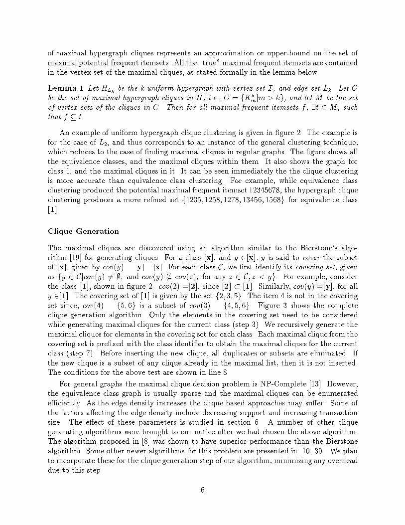
of maximal hypergraph cliques represents an approximation or upper-bound on the set ofmaximal potential frequent itemsets. All the \true" maximal frequent itemsets are containedin the vertex set of the maximal cliques, as stated formally in the lemma below.Lemma 1 Let HLk be the k-uniform hypergraph with vertex set I, and edge set Lk. Let Cbe the set of maximal hypergraph cliques in H, i.e., C = fKkmjm > kg, and let M be the setof vertex sets of the cliques in C. Then for all maximal frequent itemsets f , 9t 2 M , suchthat f � t.An example of uniform hypergraph clique clustering is given in �gure 2. The example isfor the case of L2, and thus corresponds to an instance of the general clustering technique,which reduces to the case of �nding maximal cliques in regular graphs. The �gure shows allthe equivalence classes, and the maximal cliques within them. It also shows the graph forclass 1, and the maximal cliques in it. It can be seen immediately the the clique clusteringis more accurate than equivalence class clustering. For example, while equivalence classclustering produced the potential maximal frequent itemset 12345678, the hypergraph cliqueclustering produces a more re�ned set f1235; 1258; 1278; 13456; 1568g for equivalence class[1].Clique GenerationThe maximal cliques are discovered using an algorithm similar to the Bierstone's algo-rithm [19] for generating cliques. For a class [x], and y 2[x], y is said to cover the subsetof [x], given by cov(y) = [y] \ [x]. For each class C, we �rst identify its covering set, givenas fy 2 Cjcov(y) 6= ;; and cov(y) 6� cov(z); for any z 2 C; z < yg. For example, considerthe class [1], shown in �gure 2. cov(2) =[2], since [2] � [1]. Similarly, cov(y) =[y], for ally 2[1]. The covering set of [1] is given by the set f2; 3; 5g. The item 4 is not in the coveringset since, cov(4) = f5; 6g is a subset of cov(3) = f4; 5; 6g. Figure 3 shows the completeclique generation algorithm. Only the elements in the covering set need to be consideredwhile generating maximal cliques for the current class (step 3). We recursively generate themaximal cliques for elements in the covering set for each class. Each maximal clique from thecovering set is pre�xed with the class identi�er to obtain the maximal cliques for the currentclass (step 7). Before inserting the new clique, all duplicates or subsets are eliminated. Ifthe new clique is a subset of any clique already in the maximal list, then it is not inserted.The conditions for the above test are shown in line 8.For general graphs the maximal clique decision problem is NP-Complete [13]. However,the equivalence class graph is usually sparse and the maximal cliques can be enumeratede�ciently. As the edge density increases the clique based approaches may su�er. Some ofthe factors a�ecting the edge density include decreasing support and increasing transactionsize. The e�ect of these parameters is studied in section 6. A number of other cliquegenerating algorithms were brought to our notice after we had chosen the above algorithm.The algorithm proposed in [8] was shown to have superior performance than the Bierstonealgorithm. Some other newer algorithms for this problem are presented in [10, 30]. We planto incorporate these for the clique generation step of our algorithm, minimizing any overheaddue to this step. 6

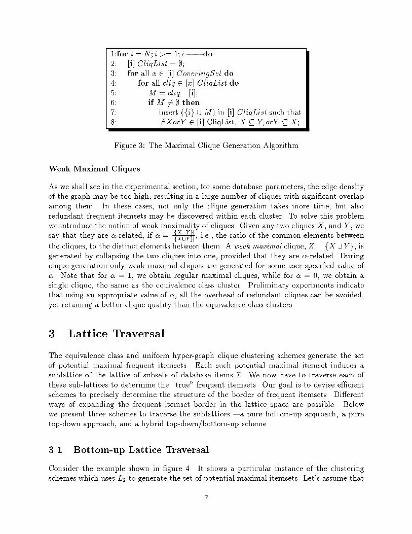
1:for i = N ; i >= 1; i�� do2: [i].CliqList = ;;3: for all x 2 [i].CoveringSet do4: for all cliq 2 [x].CliqList do5: M = cliq \ [i];6: if M 6= ; then7: insert (fig [M) in [i].CliqList such that8: 6 9XorY 2 [i].CliqList, X � Y; orY � X;Figure 3: The Maximal Clique Generation AlgorithmWeak Maximal CliquesAs we shall see in the experimental section, for some database parameters, the edge densityof the graph may be too high, resulting in a large number of cliques with signi�cant overlapamong them. In these cases, not only the clique generation takes more time, but alsoredundant frequent itemsets may be discovered within each cluster. To solve this problemwe introduce the notion of weak maximality of cliques. Given any two cliques X, and Y , wesay that they are �-related, if � = jfX\Y gjjfX[Y gj , i.e., the ratio of the common elements betweenthe cliques, to the distinct elements between them. A weak maximal clique, Z = fX [Y g, isgenerated by collapsing the two cliques into one, provided that they are �-related. Duringclique generation only weak maximal cliques are generated for some user speci�ed value of�. Note that for � = 1, we obtain regular maximal cliques, while for � = 0, we obtain asingle clique, the same as the equivalence class cluster. Preliminary experiments indicatethat using an appropriate value of �, all the overhead of redundant cliques can be avoided,yet retaining a better clique quality than the equivalence class clusters.3 Lattice TraversalThe equivalence class and uniform hyper-graph clique clustering schemes generate the setof potential maximal frequent itemsets. Each such potential maximal itemset induces asublattice of the lattice of subsets of database items I. We now have to traverse each ofthese sub-lattices to determine the \true" frequent itemsets. Our goal is to devise e�cientschemes to precisely determine the structure of the border of frequent itemsets. Di�erentways of expanding the frequent itemset border in the lattice space are possible. Belowwe present three schemes to traverse the sublattices { a pure bottom-up approach, a puretop-down approach, and a hybrid top-down/bottom-up scheme.3.1 Bottom-up Lattice TraversalConsider the example shown in �gure 4. It shows a particular instance of the clusteringschemes which uses L2 to generate the set of potential maximal itemsets. Let's assume that7

12

1245612345 13456

1234 1235 1236

1235612346

1245

1516 13 14

1246 1256

124 126

12 13 14

16 13 14 12

15Support

BOTTOM-UP TRAVERSAL

TOP-DOWN TRAVERSAL

HYBRID TRAVERSAL

Cluster: Potential Maximal Frequent Itemset (123456)

True Maximal Frequent Itemsets: 1235, 13456

Itemset 16150 200 400 500300

15

Sort Itemsets by Support

Top-Down Phase

Bottom-Up Phase

12

1235

126 125 123 124

14

156

1356

13456

123456

16 15 13

135 136 145 156146

12

134123 124 125 126

13

13456

123456

1345

14 15 16

1235 145613561346

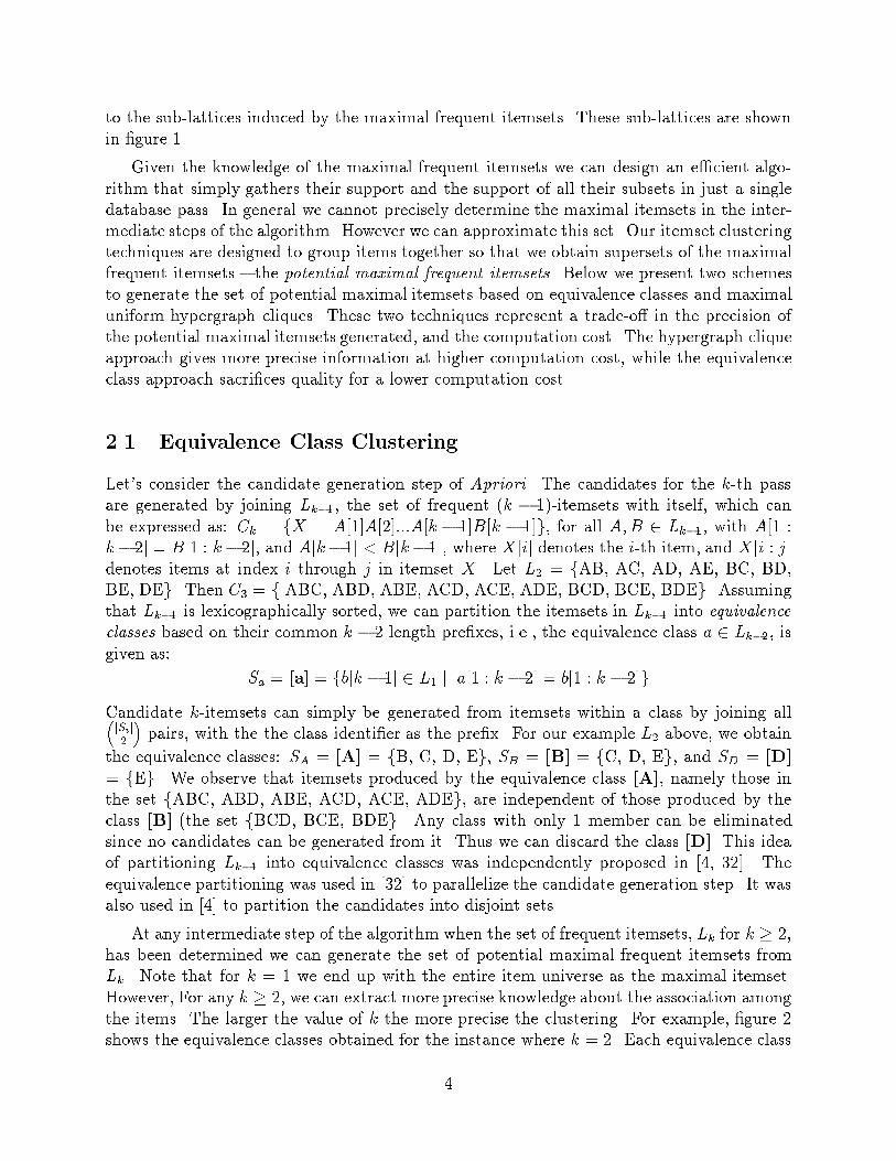
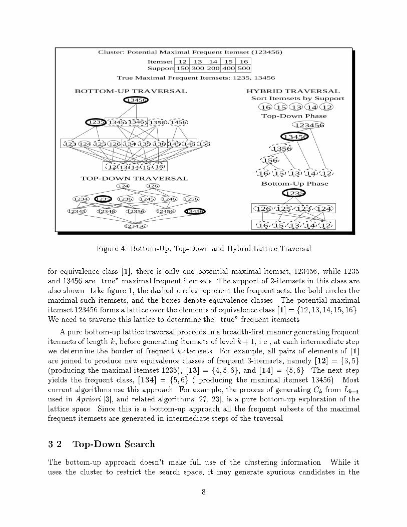
Figure 4: Bottom-Up, Top-Down and Hybrid Lattice Traversalfor equivalence class [1], there is only one potential maximal itemset, 123456, while 1235and 13456 are \true" maximal frequent itemsets. The support of 2-itemsets in this class arealso shown. Like �gure 1, the dashed circles represent the frequent sets, the bold circles themaximal such itemsets, and the boxes denote equivalence classes. The potential maximalitemset 123456 forms a lattice over the elements of equivalence class [1] = f12; 13; 14; 15; 16g.We need to traverse this lattice to determine the \true" frequent itemsets.A pure bottom-up lattice traversal proceeds in a breadth-�rst manner generating frequentitemsets of length k, before generating itemsets of level k+1, i.e., at each intermediate stepwe determine the border of frequent k-itemsets. For example, all pairs of elements of [1]are joined to produce new equivalence classes of frequent 3-itemsets, namely [12] = f3; 5g(producing the maximal itemset 1235), [13] = f4; 5; 6g, and [14] = f5; 6g. The next stepyields the frequent class, [134] = f5; 6g ( producing the maximal itemset 13456). Mostcurrent algorithms use this approach. For example, the process of generating Ck from Lk�1used in Apriori [3], and related algorithms [27, 23], is a pure bottom-up exploration of thelattice space. Since this is a bottom-up approach all the frequent subsets of the maximalfrequent itemsets are generated in intermediate steps of the traversal.3.2 Top-Down SearchThe bottom-up approach doesn't make full use of the clustering information. While ituses the cluster to restrict the search space, it may generate spurious candidates in the8

intermediate steps, since the fact that all subsets of an itemset are frequent doesn't guaranteethat the itemset is frequent. For example, the itemsets 124 and 126 in �gure 4 are infrequent,even though 12, 14, and 16 are frequent. We can envision other traversal techniques whichquickly identify the set of true maximal frequent itemsets. Once this set is known we caneither choose to stop at this point if we are interested in only the maximal itemsets, or wecan gather the support of all their subsets as well (all subsets are known to be frequentby de�nition). In this paper we will restrict our attention to only identifying the maximalfrequent subsets.One possible approach is to perform a pure top-down traversal on each cluster or sublat-tice. This schememay be thought of as trying to determine the border of infrequent itemsets,by starting at the top element of the lattice and working our way down. For example, con-sider the potential maximal frequent itemset 123456 in �gure 4. If it turns out to be frequentwe are done. But in this case it is not frequent, so we then have to check whether each of its5-subsets is frequent. At any step, if a k-subset turns out to be frequent, we need not checkany of its subsets. On the other hand, if it turns out to be infrequent, we recursively testeach (k�1)-subset. To ensure that infrequent itemsets are not tested multiple times, we alsomaintain a hash table of infrequent itemsets. Depending on the accuracy of the potentialmaximal clusters, the top-down approach may save some intersections. In our example thetop-down approach performs only 14 intersections against the 16 done by the bottom-upapproach. However, this approach doesn't work too well in practice, since the clusters areonly an approximation of the maximal frequent itemsets, and a lot of infrequent supersetsof the \true" maximal frequent itemsets may be generated. Furthermore, it also uses hashtables, and k-way intersections instead of 2-way intersections, adding extra overhead. Wetherefore, propose a hybrid top-down and bottom-up approach that works well in practice.3.3 Hybrid Top-down/Bottom-up SearchThe basic idea behind the hybrid approach is to quickly determine the \true" maximal item-sets, by starting with a single element from a cluster of frequent k-itemsets, and extendingthis by one more itemset till we generate an infrequent itemset. This comprises the top-downphase. In the bottom-up phase, the remaining elements are combined with the elements inthe �rst set to generate all the additional frequent itemsets. An important consideration inthe top-down phase is to determine which elements of the cluster should be combined. Inour approach we �rst sort the itemsets in the cluster in descending order of their support.We start with the element with maximum support, and extend it with the next element inthe sorted order. This approach is based on the intuition that the larger the support themore the likely is the itemset to be a part of a larger itemset. Figure 4 shows an example ofthe hybrid scheme on a cluster of 2-itemsets. We sort the 2-itemsets in decreasing order ofsupport, intersecting 16 and 15 to produce 156. This is extended to 1356 by joining 156 with13, and then to 13456, and �nally we �nd that 123456 is infrequent. The only remainingelement is 12. We simply join this with each of the other elements producing the frequentitemset class [12], which generates the other maximal itemset 1235. The bottom-up, top-down, and hybrid approaches are contrasted in �gure 4, and the pseudo-code for all theschemes is shown in �gure 5. 9

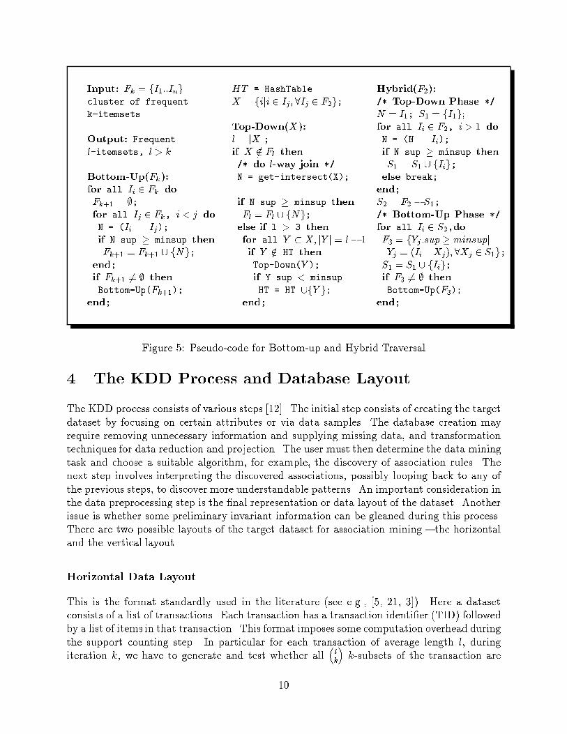
Input: Fk = fI1::Ingcluster of frequentk-itemsets.Output: Frequentl-itemsets, l > kBottom-Up(Fk):for all Ii 2 Fk doFk+1 = ;;for all Ij 2 Fk, i < j doN = (Ii \ Ij);if N.sup � minsup thenFk+1 = Fk+1 [ fNg;end;if Fk+1 6= ; thenBottom-Up(Fk+1);end;HT = HashTableX = fiji 2 Ij ; 8Ij 2 F2g;Top-Down(X):l = jX j;if X =2 Fl then/* do l-way join */N = get-intersect(X);if N.sup � minsup thenFl = Fl [ fNg;else if l > 3 thenfor all Y � X; jY j = l� 1if Y =2 HT thenTop-Down(Y );if Y.sup < minsupHT = HT [fY g;end;

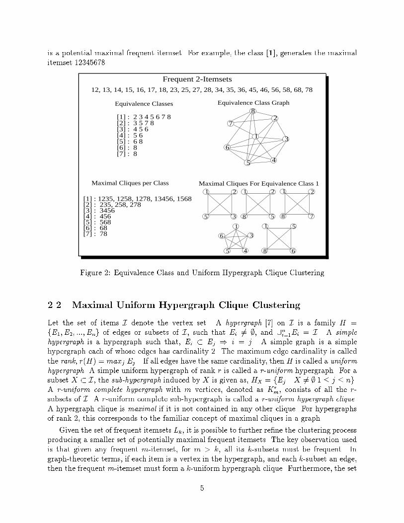
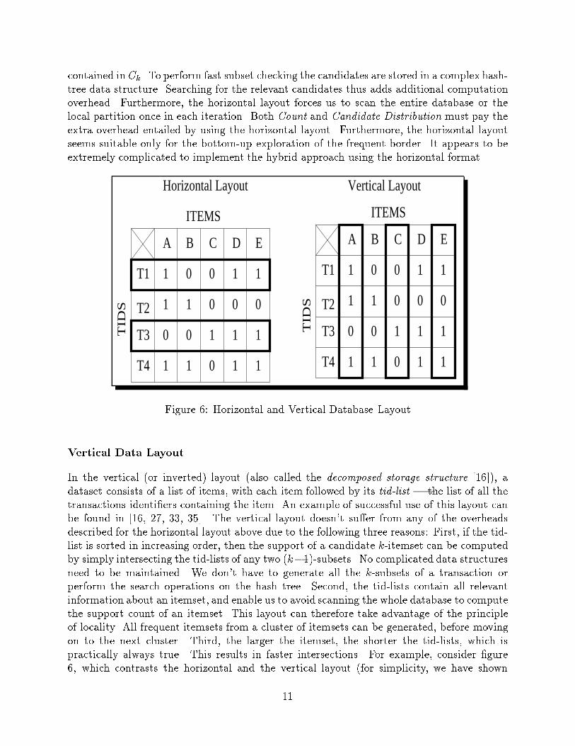
Hybrid(F2):/* Top-Down Phase */N = I1; S1 = fI1g;for all Ii 2 F2, i > 1 doN = (N \ Ii);if N.sup � minsup thenS1 = S1 [ fIig;else break;end;S2 = F2 � S1;/* Bottom-Up Phase */for all Ii 2 S2,doF3 = fYj :sup � minsupjYj = (Ii \Xj); 8Xj 2 S1g;S1 = S1 [ fIig;if F3 6= ; thenBottom-Up(F3);end;Figure 5: Pseudo-code for Bottom-up and Hybrid Traversal4 The KDD Process and Database LayoutThe KDD process consists of various steps [12]. The initial step consists of creating the targetdataset by focusing on certain attributes or via data samples. The database creation mayrequire removing unnecessary information and supplying missing data, and transformationtechniques for data reduction and projection. The user must then determine the data miningtask and choose a suitable algorithm, for example, the discovery of association rules. Thenext step involves interpreting the discovered associations, possibly looping back to any ofthe previous steps, to discover more understandable patterns. An important consideration inthe data preprocessing step is the �nal representation or data layout of the dataset. Anotherissue is whether some preliminary invariant information can be gleaned during this process.There are two possible layouts of the target dataset for association mining { the horizontaland the vertical layout.Horizontal Data LayoutThis is the format standardly used in the literature (see e.g., [5, 21, 3]). Here a datasetconsists of a list of transactions. Each transaction has a transaction identi�er (TID) followedby a list of items in that transaction. This format imposes some computation overhead duringthe support counting step. In particular for each transaction of average length l, duringiteration k, we have to generate and test whether all � lk� k-subsets of the transaction are10

contained in Ck. To perform fast subset checking the candidates are stored in a complex hash-tree data structure. Searching for the relevant candidates thus adds additional computationoverhead. Furthermore, the horizontal layout forces us to scan the entire database or thelocal partition once in each iteration. Both Count and Candidate Distribution must pay theextra overhead entailed by using the horizontal layout. Furthermore, the horizontal layoutseems suitable only for the bottom-up exploration of the frequent border. It appears to beextremely complicated to implement the hybrid approach using the horizontal format.A B C D E

1 0 0 1 1

1 1 0 0 0

1 1 100

1111 0

T2

T4

T1

T3

ITEMS

TID

S

A B C D E

1 0 0 1 1

1 1 0 0 0

1 1 100

1111 0

T2

T4

T1

T3

ITEMS

TID

S

Horizontal Layout Vertical Layout

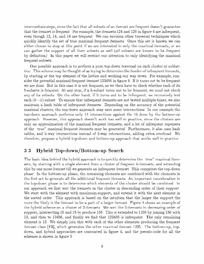
Figure 6: Horizontal and Vertical Database LayoutVertical Data LayoutIn the vertical (or inverted) layout (also called the decomposed storage structure [16]), adataset consists of a list of items, with each item followed by its tid-list | the list of all thetransactions identi�ers containing the item. An example of successful use of this layout canbe found in [16, 27, 33, 35]. The vertical layout doesn't su�er from any of the overheadsdescribed for the horizontal layout above due to the following three reasons: First, if the tid-list is sorted in increasing order, then the support of a candidate k-itemset can be computedby simply intersecting the tid-lists of any two (k�1)-subsets. No complicated data structuresneed to be maintained. We don't have to generate all the k-subsets of a transaction orperform the search operations on the hash tree. Second, the tid-lists contain all relevantinformation about an itemset, and enable us to avoid scanning the whole database to computethe support count of an itemset. This layout can therefore take advantage of the principleof locality. All frequent itemsets from a cluster of itemsets can be generated, before movingon to the next cluster. Third, the larger the itemset, the shorter the tid-lists, which ispractically always true. This results in faster intersections. For example, consider �gure6, which contrasts the horizontal and the vertical layout (for simplicity, we have shown11

the null elements, while in reality sparse storage is used). The tid-list of A, is given asT (A) = f1; 2; 4g, and T (B) = f2; 4g. Then the tid-list of AB is simply, T (AB) = f2; 4g.We can immediately determine the support by counting the number of elements in the tid-list. If it meets the minimum support criterion, we insert AB in L2. The intersections amongthe tid-lists can be performed faster by utilizing the minimum support value. For examplelet's assume that the minimum support is 100, and we are intersecting two itemsets { ABwith support 119 and AC with support 200. We can stop the intersection the moment wehave 20 mismatches in AB, since the support of ABC is bounded above by 119. We use thisoptimization, called short-circuited intersection, for fast joins.The inverted layout, however, has a drawback. Examination of small itemsets tends tobe costlier than when the horizontal layout is employed. This is because tid-lists of smallitemsets provide little information about the association among items. In particular, no suchinformation is present in the tid-lists for 1-itemsets. For example, a database with 1,000,000(1M) transactions, 1,000 frequent items, and an average of 10 items per transaction hastid-lists of average size 10,000. To �nd frequent 2-itemsets we have to intersect each pairof items, which requires �1;0002 � � (2 � 10; 000) � 109 operations. On the other hand, in thehorizontal format we simply need to form all pairs of the items appearing in a transactionand increment their count, requiring only �102 � � 1; 000; 000 = 4:5 � 107 operations.There are a number of possible solutions to this problem: 1) Use a preprocessing stepto gather the occurrence count of all 2-itemsets. Since this information is invariant, it hasto be performed once during the lifetime of the database, and the cost can be amortizedover the number of times the data is mined. This information can also be incrementallyupdated as the database changes over time. 2) Instead of storing the support counts of allthe 2-itemsets, use a user speci�ed lower bound on the minimum support the user may wishto apply. Then store the counts of only those 2-itemsets that have support greater thanthe lower bound. The idea is to minimize the storage by keeping the counts of only thoseitemsets that can be frequent, provided the user always speci�es a minimum support greaterthan the lower bound. 3) Use a small sample that would �t in memory, and determine asuperset of the frequent 2-itemsets, L2, by lowering the minimum support, and using simpleintersections on the sampled tid-lists. Sampling experiments [31, 34] indicate that this is afeasible approach. Once the superset has been determined we can easily verify the \true"frequent itemsets among them,Our current implementation uses the pre-processing approach due to its simplicity. Weplan to implement the sampling approach in a later paper. The two solutions represent atrade-o�. The sampling approach generates L2 on-the- y with an extra database pass, whilethe pre-processing approach requires extra storage. For m items, count storage requiresO(m2) disk space, which can be quite large for large values of m. However, for m = 1000,used in our experiments this adds only a very small extra storage overhead. Note also thatthe database itself requires the same amount of memory in both the horizontal and verticalformats (this is obvious from �gure 6). 12

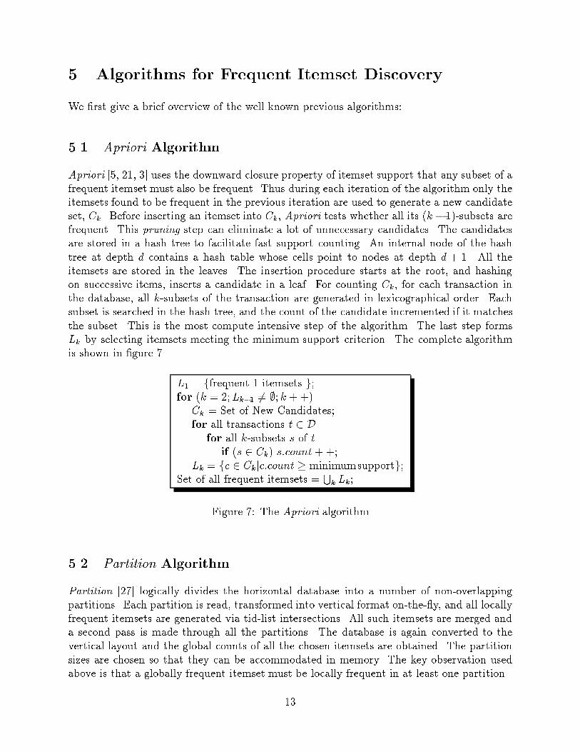
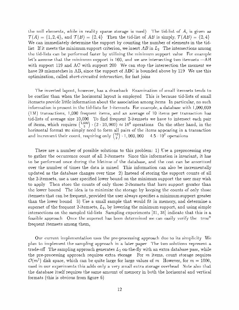
5 Algorithms for Frequent Itemset DiscoveryWe �rst give a brief overview of the well known previous algorithms:5.1 Apriori AlgorithmApriori [5, 21, 3] uses the downward closure property of itemset support that any subset of afrequent itemset must also be frequent. Thus during each iteration of the algorithm only theitemsets found to be frequent in the previous iteration are used to generate a new candidateset, Ck. Before inserting an itemset into Ck, Apriori tests whether all its (k� 1)-subsets arefrequent. This pruning step can eliminate a lot of unnecessary candidates. The candidatesare stored in a hash tree to facilitate fast support counting. An internal node of the hashtree at depth d contains a hash table whose cells point to nodes at depth d + 1. All theitemsets are stored in the leaves. The insertion procedure starts at the root, and hashingon successive items, inserts a candidate in a leaf. For counting Ck, for each transaction inthe database, all k-subsets of the transaction are generated in lexicographical order. Eachsubset is searched in the hash tree, and the count of the candidate incremented if it matchesthe subset. This is the most compute intensive step of the algorithm. The last step formsLk by selecting itemsets meeting the minimum support criterion. The complete algorithmis shown in �gure 7. L1 = ffrequent 1-itemsets g;for (k = 2;Lk�1 6= ;; k ++)Ck = Set of New Candidates;for all transactions t 2 Dfor all k-subsets s of tif (s 2 Ck) s:count++;Lk = fc 2 Ckjc:count � minimumsupportg;Set of all frequent itemsets = Sk Lk;Figure 7: The Apriori algorithm5.2 Partition AlgorithmPartition [27] logically divides the horizontal database into a number of non-overlappingpartitions. Each partition is read, transformed into vertical format on-the- y, and all locallyfrequent itemsets are generated via tid-list intersections. All such itemsets are merged anda second pass is made through all the partitions. The database is again converted to thevertical layout and the global counts of all the chosen itemsets are obtained. The partitionsizes are chosen so that they can be accommodated in memory. The key observation usedabove is that a globally frequent itemset must be locally frequent in at least one partition.13

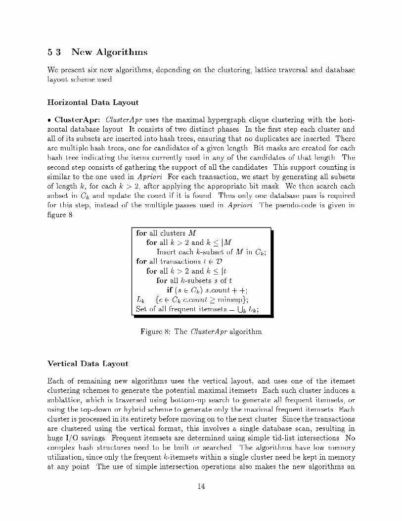
5.3 New AlgorithmsWe present six new algorithms, depending on the clustering, lattice traversal and databaselayout scheme used.Horizontal Data Layout� ClusterApr: ClusterApr uses the maximal hypergraph clique clustering with the hori-zontal database layout. It consists of two distinct phases. In the �rst step each cluster andall of its subsets are inserted into hash trees, ensuring that no duplicates are inserted. Thereare multiple hash trees, one for candidates of a given length. Bit masks are created for eachhash tree indicating the items currently used in any of the candidates of that length. Thesecond step consists of gathering the support of all the candidates. This support counting issimilar to the one used in Apriori. For each transaction, we start by generating all subsetsof length k, for each k > 2, after applying the appropriate bit mask. We then search eachsubset in Ck and update the count if it is found. Thus only one database pass is requiredfor this step, instead of the multiple passes used in Apriori. The pseudo-code is given in�gure 8. for all clusters Mfor all k > 2 and k � jM jInsert each k-subset of M in Ck;for all transactions t 2 Dfor all k > 2 and k � jtjfor all k-subsets s of tif (s 2 Ck) s:count++;Lk = fc 2 Ckjc:count � minsupg;Set of all frequent itemsets = Sk Lk;Figure 8: The ClusterApr algorithmVertical Data LayoutEach of remaining new algorithms uses the vertical layout, and uses one of the itemsetclustering schemes to generate the potential maximal itemsets. Each such cluster induces asublattice, which is traversed using bottom-up search to generate all frequent itemsets, orusing the top-down or hybrid scheme to generate only the maximal frequent itemsets. Eachcluster is processed in its entirety before moving on to the next cluster. Since the transactionsare clustered using the vertical format, this involves a single database scan, resulting inhuge I/O savings. Frequent itemsets are determined using simple tid-list intersections. Nocomplex hash structures need to be built or searched. The algorithms have low memoryutilization, since only the frequent k-itemsets within a single cluster need be kept in memoryat any point. The use of simple intersection operations also makes the new algorithms an14

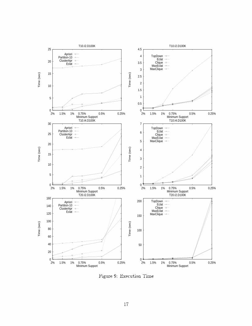
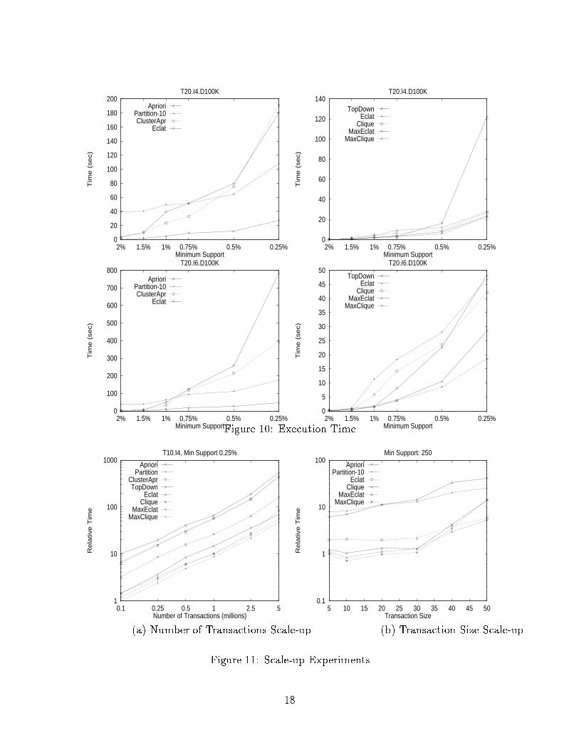
attractive option for direct implementation on general purpose database systems. The newalgorithms are:� Eclat: use equivalence class clustering along with bottom-up lattice traversal.� MaxEclat: uses equivalence class clustering along with hybrid traversal.� Clique: uses maximal hypergraph clique clustering along with bottom-up traversal� MaxClique: uses maximal hypergraph clique clustering along with hybrid lattice traversal� TopDown: uses maximal hypergraph clique clustering with top-down traversal.The pseudo-code for the maximal hypergraph clique scheme was presented in �gure 3(generating equivalence classes is quite straightforward), while the code for the three traversalstrategies was shown in �gure 5. Theses two steps combined represent the pseudo-code forthe new algorithms. We would like to note that our current implementation uses only aninstance of the general maximal hypergraph cliques technique, i.e. for the case where k = 2.We can easily envision a more dynamic scheme where we re�ne the hypergraph clustering asthe frequent k-itemsets for k > 2 become known. For example, when all 3-itemsets have beenfound within a class, we can try to get a more re�ned set of maximal 3-uniform hypergraphcliques, and so on. We plan to implement this approach in the future.6 Experimental ResultsOur experiments used a 100MHz MIPS processor with 256MB main memory, 16KB pri-mary cache, 1MB secondary cache and an attached 2GB disk. We used di�erent syntheticdatabases which mimic the transactions in a retailing environment, and were generated us-ing the procedure described in [5]. These have been used as benchmark databases for manyassociation rules algorithms [5, 16, 23, 27, 3]. The di�erent database parameters varied inour experiments are the number of transactions D, average transaction size T , and the av-erage size of a maximal potentially frequent itemset I. The number of maximal potentiallyfrequent itemsets was set at L = 2000, and the number of items at N = 1000. We refer thereader to [5] for more detail on the database generation. For fair comparison, all algorithmsdiscover frequent k-itemsets for k � 3, using the 2-itemset supports from the preprocessingstep.6.1 PerformanceIn �gures 9 and 10, we compare our new algorithms against Apriori and Partition (with10 partitions) for decreasing values of minimum support on the di�erent databases. Wecompare Eclat against Apriori, ClusterApr and Partition in the left column, and we compareEclat against the other algorithms in the right column, to highlight the di�erences amongthem. As the support decreases, the size and the number of frequent itemsets increases.Apriori thus has to make multiple passes over the database, and performs poorly. Partitionperforms worse than Apriori on small databases, and for high support, since the databaseis only scanned once or twice at these points. Partition also performs the inversion fromhorizontal to vertical tid-list format on-the- y, incurring additional overhead. However, as15

the support is lowered, Partition wins out over Apriori, since it only scans the databasetwice. It also saves some computation overhead of hash trees, since it also uses simpleintersections to compute frequent itemsets. These results are in agreement with previousexperiments comparing these two algorithms [27]. One major problem with Partition is thatas the number of partitions increases, the number of locally frequent itemsets, which arenot globally frequent, increases. While this can be reduced by randomizing the partitionselection, sampling experiments [34, 31] indicate that randomized partitions will have alarge number of frequent itemsets in common. Partition can thus spend a lot of time inperforming these redundant intersections. ClusterApr scans the database only once, and out-performs Apriori in almost all cases, and generally lies between Apriori and Partition. Moreextensive experiments on large out-of-core databases are necessary to fully compare it againstPartition. ClusterApr is very sensitive to the quality of maximal cliques that are generated.For small support, or small average maximal potential frequent itemset size I for �xed T ,or with increasing average transaction size T for �xed I, the edge density of the hypergraphincreases, consequently increasing the size of the maximal cliques. ClusterApr is unlikely toperform well under these conditions, and this is con�rmed for the T20.I2.D100K database,where it performs the worst. Like Apriori, it also maintains hash trees for support counting.Eclat performs signi�cantly better than all these algorithms in all cases. It out-performsApriori by more than an order of magnitude, and Partition by more than a factor of �ve.Eclat makes only once database scan, requires no hash trees, uses only simple intersectionoperations to generate globally frequent itemsets, avoids redundant computations, and sinceit deals with one cluster at a time, has excellent locality.Eclat Clique MaxEclat MaxClique TopDown Partition# Joins 83606 61968 56908 20322 24221 895429Time (sec) 46.7 42.1 28.5 18.5 48.2 174.7Table 1: Number of Joins: T20.I6.D100K (0.25%)The right hand columns in �gure 9 and 10 present the comparison among the other newalgorithms. Among the clustering techniques, Clique provides a �ner level of clustering, re-ducing the number of candidates considered, and therefore performs better than Eclat whenthe number of cliques considered is not too large. The graphs for MaxEclat and MaxCliqueindicate that the reduction in search space by performing the hybrid search also providessigni�cant gains. Both the maximal strategies outperform their normal counterparts. Top-Down generally speaking out-performs both Eclat and MaxEclat, since it also only generatesthe maximal frequent itemsets. As with ClusterApr, it is very sensitive to the accuracy ofthe cliques, and it su�ers as the cliques become larger. The best scheme for the databasesconsidered is MaxClique since it bene�ts from both the �ner clustering, and hybrid searchscheme. Table 1 gives the number of joins performed on T20.I2.D100K, while �gure 12provides more detail for the di�erent databases. It can be observed that MaxClique cutsdown the candidate search space drastically (more than a factor of 4 for T20.I6.D100K). Interms of raw performance MaxClique outperforms Apriori by a factor of 40 Partition by a16

0

5

10

15

20

25

2% 1.5% 1% 0.75% 0.5% 0.25%

Tim

e (

sec)

Minimum Support

T10.I2.D100K

AprioriPartition-10ClusterApr

Eclat

0

0.5

1

1.5

2

2.5

3

3.5

4

4.5

2% 1.5% 1% 0.75% 0.5% 0.25%

Tim

e (

sec)

Minimum Support

T10.I2.D100K

TopDownEclat

CliqueMaxEclat

MaxClique

0

5

10

15

20

25

30

2% 1.5% 1% 0.75% 0.5% 0.25%

Tim

e (

sec)

Minimum Support

T10.I4.D100K

AprioriPartition-10ClusterApr

Eclat

0

1

2

3

4

5

6

7

2% 1.5% 1% 0.75% 0.5% 0.25%

Tim

e (

sec)

Minimum Support

T10.I4.D100K

TopDownEclat

CliqueMaxEclat

MaxClique

0

20

40

60

80

100

120

140

160

2% 1.5% 1% 0.75% 0.5% 0.25%

Tim

e (

sec)

Minimum Support

T20.I2.D100K

AprioriPartition-10ClusterApr

Eclat

0

50

100

150

200

2% 1.5% 1% 0.75% 0.5% 0.25%

Tim

e (

sec)

Minimum Support

T20.I2.D100K

TopDownEclat

CliqueMaxEclat

MaxClique

Figure 9: Execution Time17

0

20

40

60

80

100

120

140

160

180

200

2% 1.5% 1% 0.75% 0.5% 0.25%

Tim

e (

sec)

Minimum Support

T20.I4.D100K

AprioriPartition-10ClusterApr

Eclat

0

20

40

60

80

100

120

140

2% 1.5% 1% 0.75% 0.5% 0.25%

Tim

e (

sec)

Minimum Support

T20.I4.D100K

TopDownEclat

CliqueMaxEclat

MaxClique

0

100

200

300

400

500

600

700

800

2% 1.5% 1% 0.75% 0.5% 0.25%

Tim

e (

sec)

Minimum Support

T20.I6.D100K

AprioriPartition-10ClusterApr

Eclat

0

5

10

15

20

25

30

35

40

45

50

2% 1.5% 1% 0.75% 0.5% 0.25%

Tim

e (

sec)

Minimum Support

T20.I6.D100K

TopDownEclat

CliqueMaxEclat

MaxClique

Figure 10: Execution Time1

10

100

1000

0.1 0.25 0.5 1 2.5 5

Rela

tive T

ime

Number of Transactions (millions)

T10.I4, Min Support 0.25%

AprioriPartition

ClusterAprTopDown

EclatClique

MaxEclatMaxClique

0.1

1

10

100

5 10 15 20 25 30 35 40 45 50

Rela

tive T

ime

Transaction Size

Min Support: 250

AprioriPartition-10

EclatClique

MaxEclatMaxClique

(a) Number of Transactions Scale-up (b) Transaction Size Scale-upFigure 11: Scale-up Experiments18

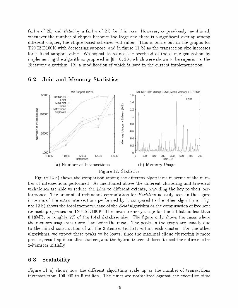
factor of 20, and Eclat by a factor of 2.5 for this case. However, as previously mentioned,whenever the number of cliques becomes too large and there is a signi�cant overlap amongdi�erent cliques, the clique based schemes will su�er. This is borne out in the graphs forT20.I2.D100K with decreasing support, and in �gure 11 b) as the transaction size increasesfor a �xed support value. We expect to reduce the overhead of the clique generation byimplementing the algorithms proposed in [8, 10, 30], which were shown to be superior to theBierstone algorithm [19], a modi�cation of which is used in the current implementation.6.2 Join and Memory Statistics1000

10000

100000

1e+06

T10.I2 T10.I4 T20.I4 T20.I6 T20.I2

Num

ber

of In

ters

ections

Databases

Min Support: 0.25%

Partition-10Eclat

MaxEclatClique

MAxCliqueTopDown

0

0.2

0.4

0.6

0.8

1

1.2

1.4

1.6

0 100 200 300 400 500 600 700

Mem

ory

Usage >

2M

ean (

MB

)

Time --->

T20.I6.D100K: Minsup 0.25%, Mean Memory = 0.018MB

Eclat

(a) Number of Intersections (b) Memory UsageFigure 12: StatisticsFigure 12 a) shows the comparison among the di�erent algorithms in terms of the num-ber of intersections performed. As mentioned above the di�erent clustering and traversaltechniques are able to reduce the joins to di�erent extents, providing the key to their per-formance. The amount of redundant computation for Partition is easily seen in the �gurein terms of the extra intersections performed by it compared to the other algorithms. Fig-ure 12 b) shows the total memory usage of the Eclat algorithm as the computation of frequentitemsets progresses on T20.I6.D100K. The mean memory usage for the tid-lists is less than0.18MB, or roughly 2% of the total database size. The �gure only shows the cases wherethe memory usage was more than twice the mean. The peaks in the graph are usually dueto the initial construction of all the 2-itemset tid-lists within each cluster. For the otheralgorithms, we expect these peaks to be lower, since the maximal clique clustering is moreprecise, resulting in smaller clusters, and the hybrid traversal doesn't need the entire cluster2-itemsets initially.6.3 ScalabilityFigure 11 a) shows how the di�erent algorithms scale up as the number of transactionsincreases from 100,000 to 5 million. The times are normalized against the execution time19

for MaxClique on 100,000 transactions. A minimum support value of 0.25% was used. Thenumber of partitions for Partition was varied from 1 to 50. While all algorithms scalelinearly, the slope is much smaller for the new algorithms. This implies that the performancedi�erences for larger databases, across algorithms is likely to increase. Figure 11 b) showshow the di�erent algorithms scale with increasing transaction size. The times are normalizedagainst the execution time for MaxClique on T = 5 and 200,000 transactions. Instead of apercentage, we used an absolute support of 250. The physical size of the database was keptroughly the same by keeping a constant T �D value. We used D = 200; 000 for T = 5, andD = 20; 000 for T = 50. There is a gradual increase in execution time for all algorithmswith increasing transaction size. However the new algorithms again outperform Apriori andPartition. As the transaction size increases, the number of cliques increases, and the cliquebased algorithms start performing worse.7 ConclusionsIn this paper we proposed new algorithms for association mining and evaluate their e�ective-ness. The proposed algorithms scan the preprocessed database exactly once, greatly reducingI/O costs. Three main techniques are employed in these algorithms. We �rst cluster itemsetsusing equivalence classes or maximal hypergraph cliques to obtain a set of potential maximalfrequent itemsets. We then generate the true frequent itemsets from each cluster sublatticeusing bottom-up, top-down or hybrid lattice traversal. Two di�erent database layout arestudied { the horizontal or the vertical format. Experimental results indicate more than anorder of magnitude improvements over previous algorithms.

20

References[1] R. Agrawal, T. Imielinski, and A. Swami. Database mining: A performance perspective.In IEEE Trans. on Knowledge and Data Engg., pages 5(6):914{925, 1993.[2] R. Agrawal, T. Imielinski, and A. Swami. Mining association rules between sets of itemsin large databases. In ACM SIGMOD Intl. Conf. Management of Data, May 1993.[3] R. Agrawal, H. Mannila, R. Srikant, H. Toivonen, and A. I. Verkamo. Fast discoveryof association rules. In U. Fayyad and et al, editors, Advances in Knowledge Discoveryand Data Mining. MIT Press, 1996.[4] R. Agrawal and J. Shafer. Parallel mining of association rules. In IEEE Trans. onKnowledge and Data Engg., pages 8(6):962{969, 1996.[5] R. Agrawal and R. Srikant. Fast algorithms for mining association rules. In 20th VLDBConf., Sept. 1994.[6] R. Agrawal and R. Srikant. Mining sequential patterns. In Intl. Conf. on Data Engg.,1995.[7] C. Berge. Hypergraphs: Combinatorics of Finite Sets. North-Holland, 1989.[8] C. Bron and J. Kerbosch. Finding all cliques of an undirected graph. In Communica-tions of the ACM, 16(9):575-577, Sept. 1973.[9] S. Brin, R. Motwani, J. Ullman, and S. Tsur. Dynamic itemset counting and implicationrules for market basket data. In ACM SIGMOD Conf. Management of Data, May 1997.[10] N. Chiba and T. Nishizeki. Arboricity and subgraph listing algorithms. In SIAM J.Computing, 14(1):210-223, Feb. 1985.[11] D. Cheung, V. Ng, A. Fu, and Y. Fu. E�cient mining of association rules in distributeddatabases. In IEEE Trans. on Knowledge and Data Engg., pages 8(6):911{922, 1996.[12] U. Fayyad, G. Piatetsky-Shapiro, and P. Smyth. The KDD process for extracting usefulknowledge from volumes of data. In Communications of the ACM { Data Mining andKnowledge Discovery in Databases, Nov. 1996.[13] M. R. Garey and D. S. Johnson. Computers and Intractability: A Guide to the Theoryof NP-Completeness. W. H. Freeman and Co., 1979.[14] E.-H. Han, G. Karypis, and V. Kumar. Scalable parallel data mining for associationrules. In ACM SIGMOD Conf. Management of Data, May 1997.[15] J. Han and Y. Fu. Discovery of multiple-level association rules from large databases.In 21st VLDB Conf., 1995. 21

[16] M. Holsheimer, M. Kersten, H. Mannila, and H. Toivonen. A perspective on databasesand data mining. In 1st Intl. Conf. Knowledge Discovery and Data Mining, Aug. 1995.[17] M. Houtsma and A. Swami. Set-oriented mining of association rules in relationaldatabases. In 11th Intl. Conf. Data Engineering, 1995.[18] M. Klemettinen, H. Mannila, P. Ronkainen, H. Toivonen, and A. I. Verkamo. Find-ing interesting rules from large sets of discovered association rules. In 3rd Intl. Conf.Information and Knowledge Management, pages 401{407, Nov. 1994.[19] G. D. Mulligan and D. G. Corneil. Corrections to Bierstone's Algorithm for GeneratingCliques. In J. Association of Computing Machinery, 19(2):244-247, Apr. 1972.[20] H. Mannila and H. Toivonen. Discovering generalized episodes using minimal oc-curences. In 2nd Intl. Conf. Knowledge Discovery and Data Mining, 1996.[21] H. Mannila, H. Toivonen, and I. Verkamo. E�cient algorithms for discovering associa-tion rules. In AAAI Wkshp. Knowledge Discovery in Databases, July 1994.[22] H. Mannila, H. Toivonen, and I. Verkamo. Discovering frequent episodes in sequences.In 1st Intl. Conf. Knowledge Discovery and Data Mining, 1995.[23] J. S. Park, M. Chen, and P. S. Yu. An e�ective hash based algorithm for miningassociation rules. In ACM SIGMOD Intl. Conf. Management of Data, May 1995.[24] J. S. Park, M. Chen, and P. S. Yu. E�cient parallel data mining for association rules.In ACM Intl. Conf. Information and Knowledge Management, Nov. 1995.[25] S. Parthasarathy, M. J. Zaki, and W. Li. Application driven memory placement fordynamic data structures. Technical Report URCS TR 653, University of Rochester,Apr. 1997.[26] G. Piatetsky-Shapiro. Discovery, presentation and analysis of strong rules. In G. P.-S.et al, editor, KDD. AAAI Press, 1991.[27] A. Savasere, E. Omiecinski, and S. Navathe. An e�cient algorithm for mining associa-tion rules in large databases. In 21st VLDB Conf., 1995.[28] R. Srikant and R. Agrawal. Mining quantitative association rules in large relationaltables. In ACM SIGMOD Conf. Management of Data, June 1996.[29] R. Srikant and R. Agrawal. Mining sequential patterns: Generalizations and perfor-mance improvements. In 5th Intl. Conf. Extending Database Technology, Mar. 1996.[30] S. Tsukiyama, M. Ide, H. Ariyoshi, and I. Shirakawa. A new algorithm for generatingall the maximal independent sets. In SIAM J. Computing, 6(3):505-517, Sept. 1977.[31] H. Toivonen. Sampling large databases for association rules. In 22nd VLDB Conf.,1996. 22

[32] M. J. Zaki, M. Ogihara, S. Parthasarathy, and W. Li. Parallel data mining for associa-tion rules on shared-memory multi-processors. In Supercomputing'96, Nov. 1996.[33] M. J. Zaki, S. Parthasarathy, and W. Li. A localized algorithm for parallel associationmining. In 9th ACM Symp. Parallel Algorithms and Architectures, June 1997.[34] M. J. Zaki, S. Parthasarathy, W. Li, and M. Ogihara. Evaluation of sampling for datamining of association rules. In 7th Intl. Wkshp. Research Issues in Data Engg, Apr.1997.[35] M. J. Zaki, S. Parthasarathy, M. Ogihara, and W. Li. New algorithms for fast discoveryof association rules. In 3rd Intl. Conf. on Knowledge Discovery and Data Mining, Aug.1997.

23