Neuromimetic Sound Representation for Percept Detection and

Manipulation †

Dmitry N. Zotkin and Ramani Duraiswami

Perceptual Interfaces and Reality Lab,Institute for Advanced Computer Studies (UMIACS),

University of Maryland at College Park, College Park, MD 20742 USA

Taishih Chi and Shihab A. Shamma

Neural Systems Laboratory, Institute of Systems Research,University of Maryland at College Park, College Park, MD 20742 USA

Abstract

The acoustic wave received at the ears is processed by the human auditory system to separate different

sounds along the intensity, pitch and timbre dimensions. Conventional Fourier-based signal processing,

while endowed with fast algorithms, is unable to easily represent a signal along these attributes. In this

paper we discuss the creation of maximally separable sounds in auditory user interfaces and use a recently

proposed cortical representation that achieves a biomimetic separation to represent and manipulate sound

for this purpose. We briefly overview algorithms for obtaining, manipulating and inverting a cortical rep-

resentation of a sound and describe algorithms for manipulating signal pitch and timbre separately. The

algorithms are also used to create sound of an instrument between a “guitar” and a “trumpet”. Excellent

sound quality can be achieved if processing time is not a concern, and intelligible signals can be recon-

structed in reasonable processing time (about ten seconds of computational time for a one second signal

sampled at 8 kHz). Work on bringing the algorithms into the real-time processing domain is ongoing.

†This paper is an extended version of paper [1].

1

2

I. INTRODUCTION

When a natural sound source such as a human voice or a musical instrument produces a sound,

the resulting acoustic wave is generated by a time-varying excitation pattern of a possibly time-

varying acoustical system, and the sound characteristics depend both on the excitation signal and

on the production system. The production system (e.g., human vocal tract, the guitar box, or

the flute tube) has its own characteristic response. Varying the excitation parameters produces a

sound signal that has different frequency components, but still retains perceptual characteristics

that uniquely identify the production instrument (identity of the person, type of instrument – piano,

violin, etc.), and even the specific type of piano on which it was produced. When one is asked

to characterize this sound source using descriptions based on Fourier analysis one discovers that

concepts such as frequency and amplitude are insufficient to explain such perceptual characteristics

of the sound source. Human linguistic descriptions that characterize the sound are expressed in

terms of pitch and timbre. The goal of anthropomorphic algorithms is to reproduce these percepts

quantitatively.

The perceived sound pitch is closely coupled with its harmonic structure and frequency of the

first harmonic, or F0. On the other hand, the timbre of the sound is defined broadly as everything

other than the pitch, loudness, and the spatial location of the sound. For example, two musical

instruments might have the same pitch if they play the same note, but it is their differing timbre

that allows us to distinguish between them. Specifically, the spectral envelope and the spectral

envelope variations in time including, in particular, onset and offset properties of the sound are

related to the timbre percept.

Most conventional techniques of sound manipulation result in simultaneous changes in both

the pitch and the timbre and cannot be used to control or assess the effects in pitch and timbre

dimensions independently. A goal of this paper is the development of controls for independent

manipulation of pitch and timbre of a sound source using a cortical sound representation intro-

duced in [2], where it was used for assessment of speech intelligibility and for prediction of the

cortical response to an arbitrary stimulus, and later extended in [3] providing fuller mathematical

3

details as well as addressing invertibility issues. We simulate the multiscale audio representation

and processing believed to occur in the primate brain (supported by recent psychophysiological

papers [4]), and while our sound decomposition is partially similar to existing pitch and timbre

separation and sound morphing algorithms (in particular, MFCC decomposition algorithm in [5],

sinusoid plus noise model and effects generated with it in [6], and parametric source models using

LPC and physics-based synthesis in [7]), the neuromorphic framework provides a view of process-

ing from a different perspective, supplies supporting evidence to justify the procedure performed

and tailors it to the way the human nervous system processes auditory information, and extends

the approach to include decomposition in the time domain in addition to frequency. We anticipate

our algorithms to be applicable in several areas, including musical synthesis, audio user interfaces

and sonification.

In section 2, we discuss the potential applications for the developed framework. In sections

3 and 4, we describe the processing of the audio information through the cortical model [3] in

forward and backward directions, respectively, and in section 5 we propose an alternative, faster

implementation of the most time-consuming cortical processing stage. We discuss the quality of

audio signal reconstruction in section 6 and show examples of timbre-preserving pitch manipula-

tion of speech and timbre interpolation of musical notes in sections 7 and 8, respectively. Finally,

section 9 concludes the paper.

II. APPLICATIONS

The direct application that motivated us to undertake the research described (and the area it is

currently being used in) is the development of advanced auditory user interfaces. Auditory user

interfaces can be broadly divided into two groups, based on whether speech or non-speech audio

signals are used in the interface. The field of sonification [8] (“... use of non-speech audio to

convey information”) presents multiple challenges to researchers in that they must both identify

and manipulate different percepts of sound to represent different parameters in a data stream while

at the same time creating efficient and intuitive mappings of the data from the numerical domain

4

to the acoustical domain. An extensive resource describing sonification work is the International

Community for Auditory Display (ICAD) web page [9], which includes past conference proceed-

ings. While there are some isolated examples of useful sonifications and attempts at creating

multi-dimensional audio interfaces (e.g. the Geiger counter or the pulse-oxymeter [10]), the field

of sonification, and as a consequence audio user interfaces, is still in the infancy due to the lack of

a comprehensive theory of sonification [11].

What is needed for advancements in this area are: identification of perceptually valid attributes

(“dimensions”) of sound that can be controlled; theory and algorithms for sound manipulation

that allow control of these dimensions; psychophysical proof that these control dimensions convey

information to a human observer; methods for easy-to-understand data mapping to auditory do-

main; technology to create user interfaces using these manipulations; and refinement of acoustic

user interfaces to perform some specific example tasks. Our research addresses some of these

issues and creates the basic technology for manipulation of existing sounds and synthesis of new

sounds achieving specified attributes along the perceptual dimensions. We focus on neuromorphic-

inspired processing of pitch and timbre percepts, having the location and ambience percepts de-

scribed earlier in [12]. Our real-time pitch-timbre manipulation and scene rendering algorithms

are capable of generating stable virtual acoustic objects whose attributes can be manipulated in

these perceptual dimensions.

The same set of percepts may be modified in the case when speech signals are used in audio

user interfaces. However, the purpose of percept modification in this case is not to convey in-

formation directly but rather to allow for maximally distinguishable and intelligible perception of

(possibly several simultaneous) speech streams under stress conditions using the natural neural

auditory dimensions. Applications in this area might include, for example, an audio user interface

for a soldier where multiple sound streams are to be attended to simultaneously. To our knowl-

edge, much research has been devoted to selective attention to one signal from a group [13], [14],

[15], [17], [18] (the well-known “cocktail party effect” [19]), and there have only been a limited

number of studies (e.g., [20], [21]) on how well a person can simultaneously perceive and under-

stand multiple concurrent speech streams. The general results obtained in these papers suggest

5

that increasing separation along most of the perceptual characteristics leads to improvement in

the recognition rate for several competing messages. The characteristic that provides most im-

provement is the spatial separation of the sounds, which is beyond the scope of this paper; these

spatialization techniques are well-described in [12]. Pitch was a close second, and in the section 7

of this paper we present a cortical representation based pitch manipulation algorithm, which can

be used to achieve the desired perceptual separation of the sounds. Timbre manipulations did not

result in significant improvements in recognition rate in this study, though.

Another area where we anticipate our algorithms to be applicable to is musical synthesis. Syn-

thesizers often use sampled sound that have to be pitch-shifted to produce different notes [7].

Simple resampling that was widely used in the past in commercial-grade music synthesizers pre-

serves neither the spectral nor the temporal envelope (onset and decay ratios) of an instrument.

More recent wavetable synthesizers can impose the correct temporal envelope on the sound but

may still distort the spectral envelope. The spectral and the temporal envelopes are parts of the

timbre percept, and their incorrect manipulation can lead to poor perceptual quality of the resulting

sound samples.

The timbre of the instrument usually depends on the size and the shape of the resonator; it is

interesting that for some instruments (piano, guitar) the resonator shape (which determines the

spectral envelope of the produced sound) does not change when different notes are played, and

for others (flute, trumpet) the length of resonating air column changes as the player opens differ-

ent holes in the tube to produce different notes. Timbre-preserving pitch modification algorithm

described in section 7 provides a physically correct pitch manipulation technique for instruments

with resonator shape independent of the note played. It is also possible to perform timbre interpo-

lation between sound samples; in section 8, we describe the synthesis of a new musical instrument

with the perceptual timbre lying in-between two known instruments – the guitar and the trum-

pet. The synthesis is performed in the timbre domain, and then a timbre-preserving pitch shift

described in section 7 is applied to form different notes of the new instrument. Both operations

use a cortical representation, which turned out to be extremely useful for separate manipulations

of percepts.

6

III. THE CORTICAL MODEL

In a complex acoustic environment, sources may simultaneously change their loudness, loca-

tion, timbre, and pitch. Yet, humans are able to integrate effortlessly the multitude of cues arriving

at their ears, and derive coherent percepts and judgments about each source [22]. The cortical

model is a computational model for how the brain is able to obtain these features from the acoustic

input it receives. Physiological experiments have revealed the elegant multiscale strategy devel-

oped in the mammalian auditory system for coding of spectro-temporal characteristics of the sound

[4], [23]. The primary auditory cortex (AI), which receives its input from the thalamus, employs a

multiscale representation in which the dynamic spectrum is repeatedly represented in AI at various

degrees of spectral and temporal resolution. This is accomplished by cells whose responses are

selective to a range of spectro-temporal parameters such as the local bandwidth and the symme-

try of the spectral peaks, and their onset and offset transition rates. Similarly, psychoacoustical

investigations have shed considerable light on the way we form and label sound images based on

relationships among their physical parameters [22]. A mathematical model of the early and central

stages of auditory processing in mammals was recently developed and described in [2] and [3]. It

is a basis for our work and is briefly summarized here; a full formulation of the model is available

in [3] and analysis code in form of a MATLAB toolbox (“NSL toolbox”) can be downloaded from

[24] under “publications”.

The model consists of two basic stages. The first stage of the model is an early auditory stage,

which models the transformation of the acoustic signal into an internal neural representation,

called the “auditory spectrogram”. The second is a central stage, which analyzes the spectro-

gram to estimate its spectro-temporal features, specifically its spectral and temporal modulations,

using a bank of modulation selective filters mimicking those described in the mammalian primary

auditory cortex.

The first stage, the auditory spectrogram stage, converts the audio signal s(t) into an auditory

spectrogram representation y(t, x) (where x is the frequency on a logarithmic frequency axis) and

consists of a sequence of three operations described below.

7

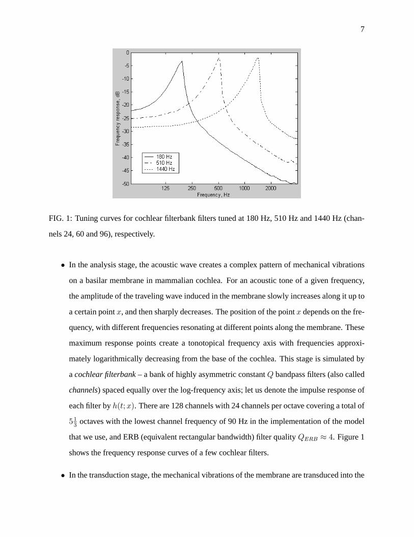
FIG. 1: Tuning curves for cochlear filterbank filters tuned at 180 Hz, 510 Hz and 1440 Hz (chan-

nels 24, 60 and 96), respectively.

• In the analysis stage, the acoustic wave creates a complex pattern of mechanical vibrations

on a basilar membrane in mammalian cochlea. For an acoustic tone of a given frequency,

the amplitude of the traveling wave induced in the membrane slowly increases along it up to

a certain point x, and then sharply decreases. The position of the point x depends on the fre-

quency, with different frequencies resonating at different points along the membrane. These

maximum response points create a tonotopical frequency axis with frequencies approxi-

mately logarithmically decreasing from the base of the cochlea. This stage is simulated by

a cochlear filterbank – a bank of highly asymmetric constant Q bandpass filters (also called

channels) spaced equally over the log-frequency axis; let us denote the impulse response of

each filter by h(t; x). There are 128 channels with 24 channels per octave covering a total of

513

octaves with the lowest channel frequency of 90 Hz in the implementation of the model

that we use, and ERB (equivalent rectangular bandwidth) filter quality QERB ≈ 4. Figure 1

shows the frequency response curves of a few cochlear filters.

• In the transduction stage, the mechanical vibrations of the membrane are transduced into the

8

intracellular potential of the inner hair cells. Membrane displacements cause flow of liquid

in the cochlea that bends the cilia (tiny hair-like formations) that are attached to the inner

hair cells. This bending opens the cell channels and enables ionic current to flow into the cell

and to change its electric potential, which is later transmitted by auditory nerve fibers to the

cochlear nucleus. In the model, these steps are simulated by a high-pass filter (equivalent to

taking a time derivative operation), nonlinear compression g(z) and then the low-pass filter

w(t) with cutoff frequency of 2 KHz, representing the fluid-cilia coupling, ionic channel

current and hair cell membrane leakage, respectively.

• Finally, in the reduction stage the input to the anteroventral cochlear nucleus undergoes

lateral inhibition operation followed by envelope detection. Lateral inhibition effectively

enhances the frequency selectivity of the cochlear filters from Q ≈ 4 to Q ≈ 12 and is

modeled by a spatial derivative across the channel array. Then, the non-negative response of

the lateral inhibitory network neurons is modeled by a half-wave rectifier, and an integration

over a short window, µ(t; τ ) = e−t/τ , with τ = 8 ms is performed to model the slow

adaptation of the central auditory neurons.

In mathematical form, three steps described above can be expressed as

y1(t, x) = s(t)⊕ h(t; x), (1)

y2(t, x) = g(∂ty1(t, x))⊕ w(t),

y(t, x) = max(∂xy2(t, x), 0)⊕ µ(t, τ),

where ⊕ denotes a convolution with respect to t.

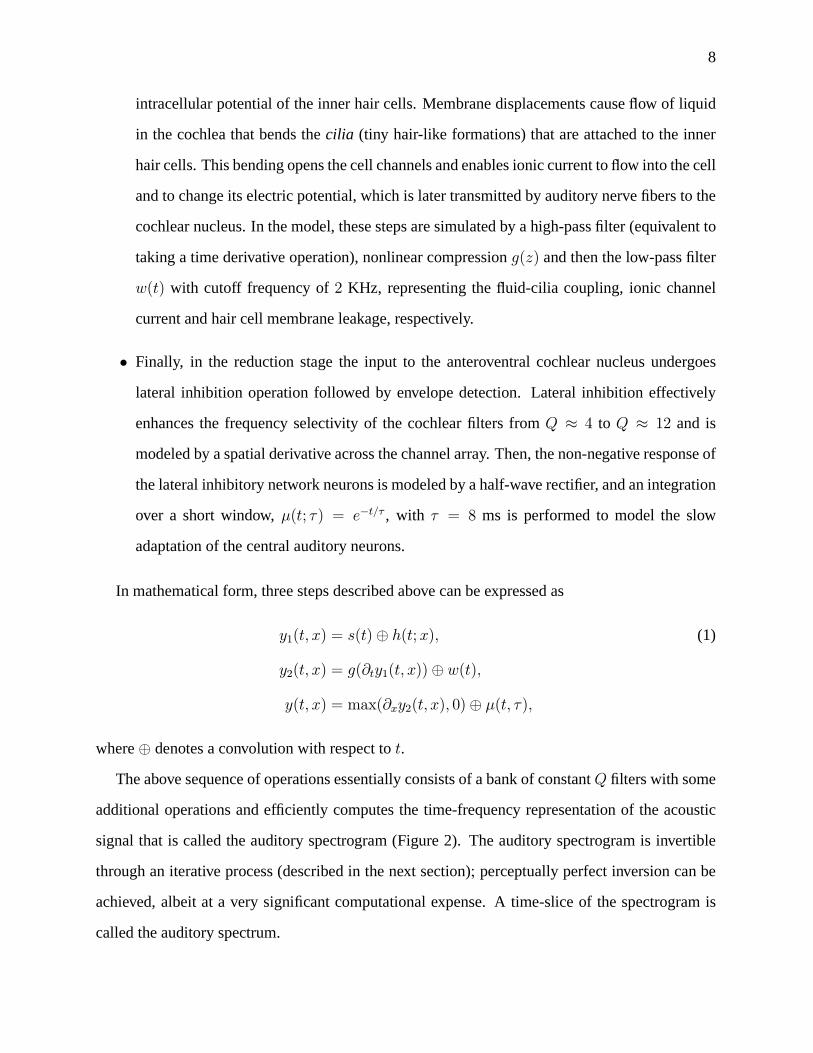
The above sequence of operations essentially consists of a bank of constantQ filters with some

additional operations and efficiently computes the time-frequency representation of the acoustic

signal that is called the auditory spectrogram (Figure 2). The auditory spectrogram is invertible

through an iterative process (described in the next section); perceptually perfect inversion can be

achieved, albeit at a very significant computational expense. A time-slice of the spectrogram is

called the auditory spectrum.

9

FIG. 2: Example auditory spectrogram for the sentence shown.

The second processing stage mimics the action of the higher central auditory stages (especially

the primary auditory cortex). We provide a mathematical derivation (as presented in [3]) of the

cortical representation below, as well as qualitatively describe the processing.

The findings of a wide variety of neuron spectro-temporal response fields (SRTF) covering

a range of frequency and temporal characteristics [23] suggests that they may, as a population,

perform a multiscale analysis of their input spectral profile. Specifically, the cortical stage esti-

mates the spectral and temporal modulation content of the auditory spectrogram using a bank of

modulation selective filters h(t, x;ω,Ω,ϕ, θ). Each filter is tuned (Q = 1) to a combination of

a particular spectral and temporal modulation of the incoming signal, and filters are centered at

different frequencies along the tonotopical axis. The two types of modulations are:

• Temporal modulation, which defines how fast the signal energy is increasing or decreasing

along the time axis at a given time and frequency. It is characterized by the parameter ω,

which is referred to as rate or velocity and measured in Hz, and by characteristic temporal

10

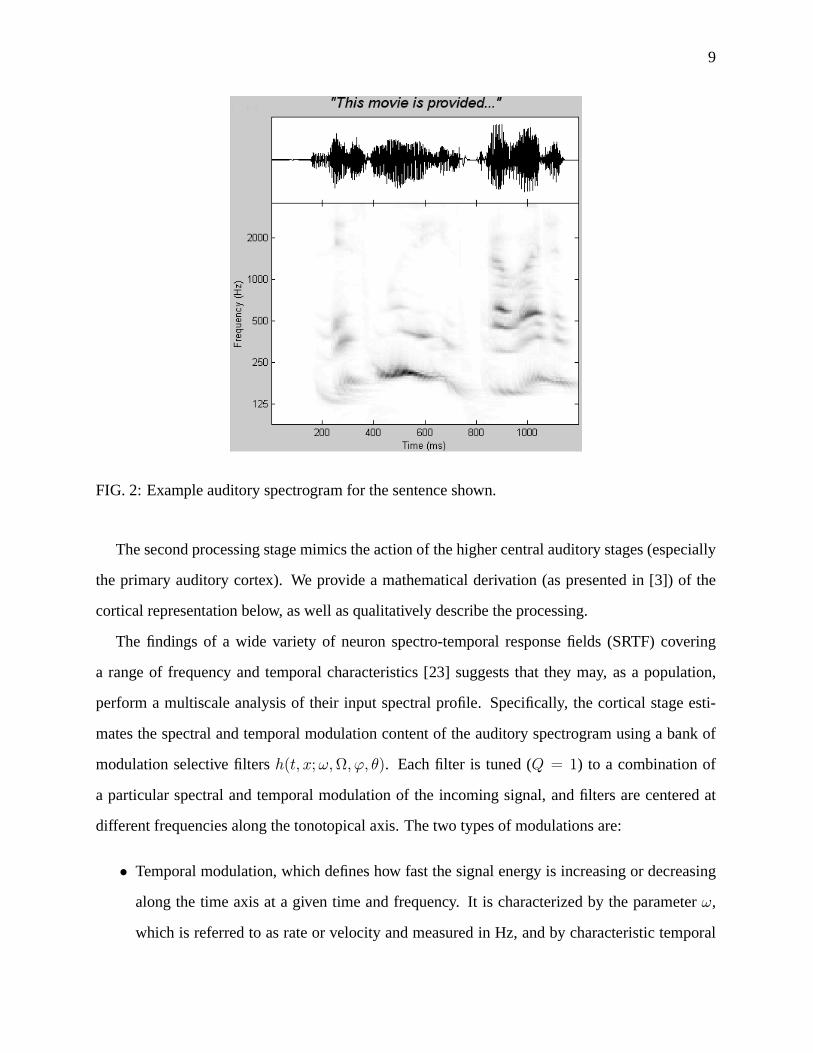
FIG. 3: Tuning curves for the basis (seed) filter for the rate-scale decomposition (scale of 1 cycle

per octave, rate of 1 Hz).

modulation phase ϕ.

• Spectral modulation, which defines how fast the signal energy varies along the frequency

axis at a given time and frequency. It is characterized by the parameter Ω, which is referred

to as density or scale and measured in cycles per octave (CPO), and by characteristic spectral

modulation phase θ.

The filters are designed for a range of rates from 2 to 32 Hz and scales from 0.25 to 8 CPO,

which corresponds to the ranges of neuron spectro-temporal response fields found in primate brain.

The impulse response function for the filter h(t, x;ω,Ω,ϕ, θ) can be factored into hs(x;Ω, θ) and

ht(t;ω,ϕ) – spectral and temporal parts, respectively. The spectral impulse response function

hs(x;Ω, θ) is defined through a phase interpolation of the spectral filter seed function u(x;Ω) with

its Hilbert transform u(x;Ω), with the similar definition for the temporal response function using

11

the temporal filter seed function v(t;ω):

hs(x;Ω, θ) = u(x;Ω) cos θ + u(x;Ω) sin θ, (2)

ht(t;ω,ϕ) = v(t;ω) cosϕ+ v(t;ω) sinϕ.

The Hilbert transform is defined as

f(x) =1

π

Z ∞

−∞

f(z)

z − xdz. (3)

We choose

u(x) = (1− x2)e−x2/2, (4)

v(t) = e−t sin(2πt)

as the functions that produce the basic seed filter tuned to a scale of 1 CPO and a rate of 1 Hz. Fig-

ure 3 shows its spectral and temporal response produced by u(x) and v(t) functions, respectively.

Differently tuned filters are obtained by dilation or compression of the filter (4) along the spectral

and temporal axes:

u(x;Ω) = Ωu(Ωx), (5)

v(t;ω) = ωv(ωt).

The response rc(t, x) of a cell c with parameters ωc,Ωc,ϕc, θc to the signal producing an audi-

tory spectrogram y(t, x) can therefore be obtained as

rc(t, x;ωc,Ωc,ϕc, θc) = y(t, x)⊗ h(t, x;ωc,Ωc,ϕc, θc), (6)

where ⊗ denotes a convolution both on x and on t.

An alternative representation of the filter can be derived in the complex domain. Denote

hs(x;Ω) = u(x;Ω) + ju(x;Ω), (7)

ht(t;ω) = v(t;ω) + jv(t;ω),

12

where j =√−1. Convolution of y(t, x) with a downward-moving STRF obtained as

hs(x;Ω)ht(t;ω) and an upward-moving SRTF obtained as hs(x;Ω)h∗t (t;ω) (where star de-

notes complex conjugation) results in two complex response functions zd(t, x;ωc,Ωc) and

zu(t, x;ωc,Ωc):

zd(t, x;ωc,Ωc) = y(t, x)⊗ [hs(x;Ωc)ht(t;ωc)] = |zd(t, x;ωc,Ωc)|ejψd(t,x;ωc,Ωc), (8)

zu(t, x;ωc,Ωc) = y(t, x)⊗ [hs(x;Ωc)h∗t (t;ωc)] = |zu(t, x;ωc,Ωc)|ejψu(t,x;ωc,Ωc),

and it can be shown [3] that

rc(t, x;ωc,Ωc,ϕc, θc) =1

2[|zd| cos(ψd − ϕc − θc) + |zu| cos(ψu + ϕc − θc)] (9)

(the arguments of zd, zu,ψd and ψu are omitted here for clarity). Thus, the complex wavelet

transform (8) uniquely determines the response of a cell with parameters ωc,Ωc,ϕc, θc to the stim-

ulus, resulting in a dimensionality reduction effect in the cortical representation. In other words,

knowledge of the complex-valued functions zd(t, x;ωc,Ωc) and zu(t, x;ωc,Ωc) fully specifies the

six-dimensional cortical representation rc(t, x;ωc,Ωc,ϕc, θc). The cortical representation thus can

be obtained by performing (8) which results in a four-dimensional (time, frequency, rate and scale)

hypercube of (complex) filter coefficients that can be manipulated as desired and inverted back into

the audio signal domain.

Essentially, the filter output is computed by a convolution of its spectro-temporal impulse re-

sponse (STIR) with the input auditory spectrogram, producing a modified spectrogram. Since the

spectral and temporal cross-sections of an STIR are typical of a bandpass impulse response in

having alternating excitatory and inhibitory fields, the output at a given time-frequency position of

the spectrogram is large only if the spectrogram modulations at that position are tuned to the rate,

scale, and direction of the STIR. A map of the responses across the filterbank provides a unique

characterization of the spectrogram that is sensitive to the spectral shape and dynamics over the

entire stimulus.

To emphasize the features of the model that are important for the current work, note that every

filter in the rate-scale analysis responds well to the auditory spectrogram features that have high

13

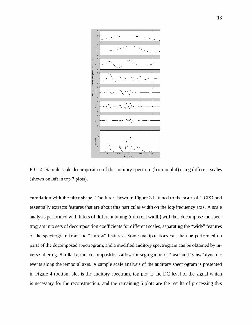
FIG. 4: Sample scale decomposition of the auditory spectrum (bottom plot) using different scales

(shown on left in top 7 plots).

correlation with the filter shape. The filter shown in Figure 3 is tuned to the scale of 1 CPO and

essentially extracts features that are about this particular width on the log-frequency axis. A scale

analysis performed with filters of different tuning (different width) will thus decompose the spec-

trogram into sets of decomposition coefficients for different scales, separating the “wide” features

of the spectrogram from the “narrow” features. Some manipulations can then be performed on

parts of the decomposed spectrogram, and a modified auditory spectrogram can be obtained by in-

verse filtering. Similarly, rate decompositions allow for segregation of “fast” and “slow” dynamic

events along the temporal axis. A sample scale analysis of the auditory spectrogram is presented

in Figure 4 (bottom plot is the auditory spectrum, top plot is the DC level of the signal which

is necessary for the reconstruction, and the remaining 6 plots are the results of processing this

14

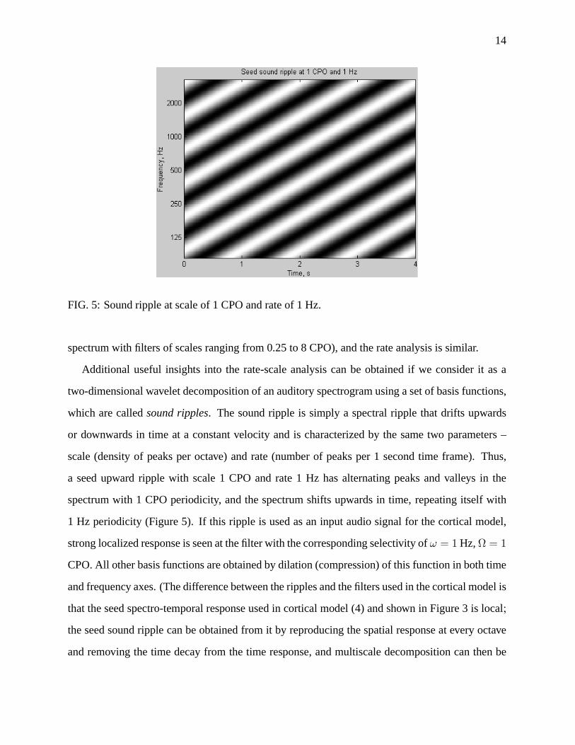
FIG. 5: Sound ripple at scale of 1 CPO and rate of 1 Hz.

spectrum with filters of scales ranging from 0.25 to 8 CPO), and the rate analysis is similar.

Additional useful insights into the rate-scale analysis can be obtained if we consider it as a

two-dimensional wavelet decomposition of an auditory spectrogram using a set of basis functions,

which are called sound ripples. The sound ripple is simply a spectral ripple that drifts upwards

or downwards in time at a constant velocity and is characterized by the same two parameters –

scale (density of peaks per octave) and rate (number of peaks per 1 second time frame). Thus,

a seed upward ripple with scale 1 CPO and rate 1 Hz has alternating peaks and valleys in the

spectrum with 1 CPO periodicity, and the spectrum shifts upwards in time, repeating itself with

1 Hz periodicity (Figure 5). If this ripple is used as an input audio signal for the cortical model,

strong localized response is seen at the filter with the corresponding selectivity of ω = 1Hz, Ω = 1

CPO. All other basis functions are obtained by dilation (compression) of this function in both time

and frequency axes. (The difference between the ripples and the filters used in the cortical model is

that the seed spectro-temporal response used in cortical model (4) and shown in Figure 3 is local;

the seed sound ripple can be obtained from it by reproducing the spatial response at every octave

and removing the time decay from the time response, and multiscale decomposition can then be

15

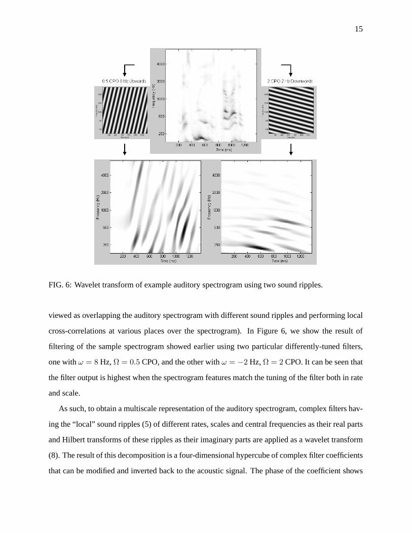
FIG. 6: Wavelet transform of example auditory spectrogram using two sound ripples.

viewed as overlapping the auditory spectrogram with different sound ripples and performing local

cross-correlations at various places over the spectrogram). In Figure 6, we show the result of

filtering of the sample spectrogram showed earlier using two particular differently-tuned filters,

one with ω = 8 Hz, Ω = 0.5 CPO, and the other with ω = −2 Hz, Ω = 2 CPO. It can be seen that

the filter output is highest when the spectrogram features match the tuning of the filter both in rate

and scale.

As such, to obtain a multiscale representation of the auditory spectrogram, complex filters hav-

ing the “local” sound ripples (5) of different rates, scales and central frequencies as their real parts

and Hilbert transforms of these ripples as their imaginary parts are applied as a wavelet transform

(8). The result of this decomposition is a four-dimensional hypercube of complex filter coefficients

that can be modified and inverted back to the acoustic signal. The phase of the coefficient shows

16

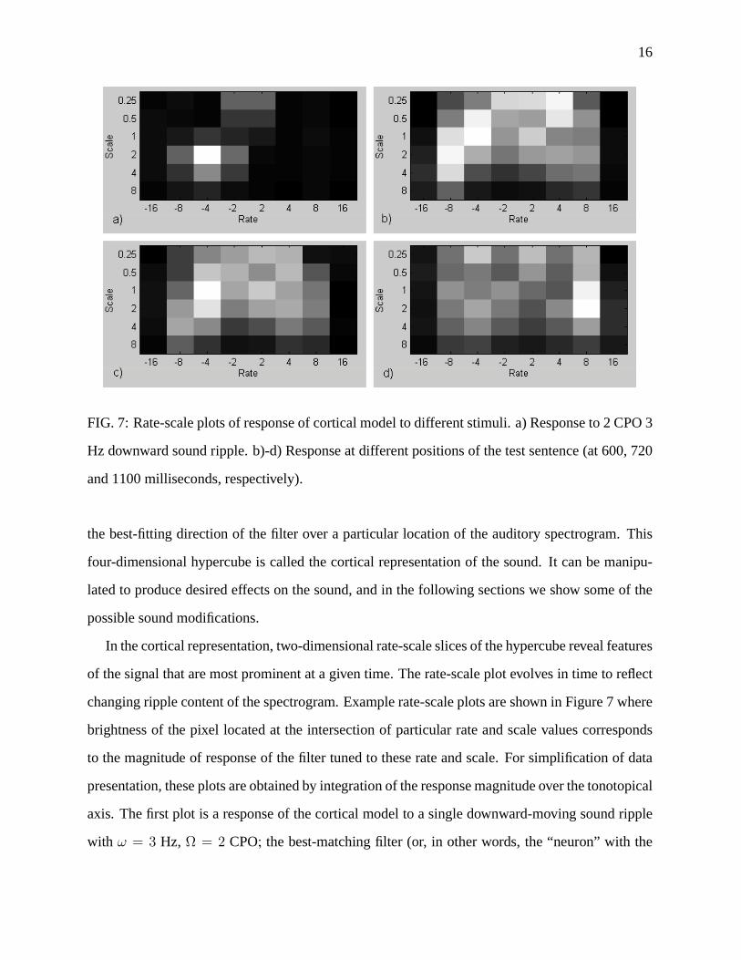
FIG. 7: Rate-scale plots of response of cortical model to different stimuli. a) Response to 2 CPO 3

Hz downward sound ripple. b)-d) Response at different positions of the test sentence (at 600, 720

and 1100 milliseconds, respectively).

the best-fitting direction of the filter over a particular location of the auditory spectrogram. This

four-dimensional hypercube is called the cortical representation of the sound. It can be manipu-

lated to produce desired effects on the sound, and in the following sections we show some of the

possible sound modifications.

In the cortical representation, two-dimensional rate-scale slices of the hypercube reveal features

of the signal that are most prominent at a given time. The rate-scale plot evolves in time to reflect

changing ripple content of the spectrogram. Example rate-scale plots are shown in Figure 7 where

brightness of the pixel located at the intersection of particular rate and scale values corresponds

to the magnitude of response of the filter tuned to these rate and scale. For simplification of data

presentation, these plots are obtained by integration of the response magnitude over the tonotopical

axis. The first plot is a response of the cortical model to a single downward-moving sound ripple

with ω = 3 Hz, Ω = 2 CPO; the best-matching filter (or, in other words, the “neuron” with the

17

corresponding SRTF) responds best. The responses of 2-Hz and 4-Hz units are not equal here

because of the cochlear filterbank asymmetry in the early stage of processing. The other three

plots show the evolution of the rate-scale response at different times during the sample auditory

spectrogram shown in Figure 2 (at approximately 600, 720, and 1100 milliseconds, respectively);

one can indeed trace the plot time stamps back to the spectrogram and see that the spectrogram has

mostly sparse downward-moving and mostly dense upward-moving features appearing before the

720 and 1100 milliseconds marks, respectively. The peaks in the test sentence plots are sharper in

rate than in scale, which can be explained by the integration performed over the tonotopical axis

in these plots (the speech signal is anyway unlikely to elicit significantly different rate-scale maps

at different frequencies because it consists mostly of equispaced harmonics which can rise or fall

only in unison, so the prevalent rate is not likely to differ at different points on the tonotopical axis;

the prevalent scale though does change somewhat due to higher number of harmonics per octave

towards higher frequencies).

IV. RECONSTRUCTING THE AUDIO FROM THE MODEL

After altering the cortical representation, it is necessary to reconstruct the modified audio sig-

nal. Just as with the forward path, the reconstruction consists of central stage and early stage. The

first step is the inversion of the cortical multiscale representation back to a spectrogram. This is

critical, since the timbre and pitch manipulations are easier to do in the cortical domain. This is

a one step inverse wavelet transform operation because of the linear nature of the transform (8),

which in the Fourier domain can be written as

Zd(ω,Ω;ωc,Ωc) = Y (ω,Ω)Hs(Ω;Ωc)Ht(ω;ωc), (10)

Zu(ω,Ω;ωc,Ωc) = Y (ω,Ω)Hs(Ω;Ωc)H∗t (−ω;ωc).

where capital letters signify the Fourier transforms of the functions determined by the correspond-

ing lowercase letters. From (10), similarly to the usual Fourier transform case, one can write

the formula for the Fourier transform of the reconstructed auditory spectrogram yr(t, x) from its

18

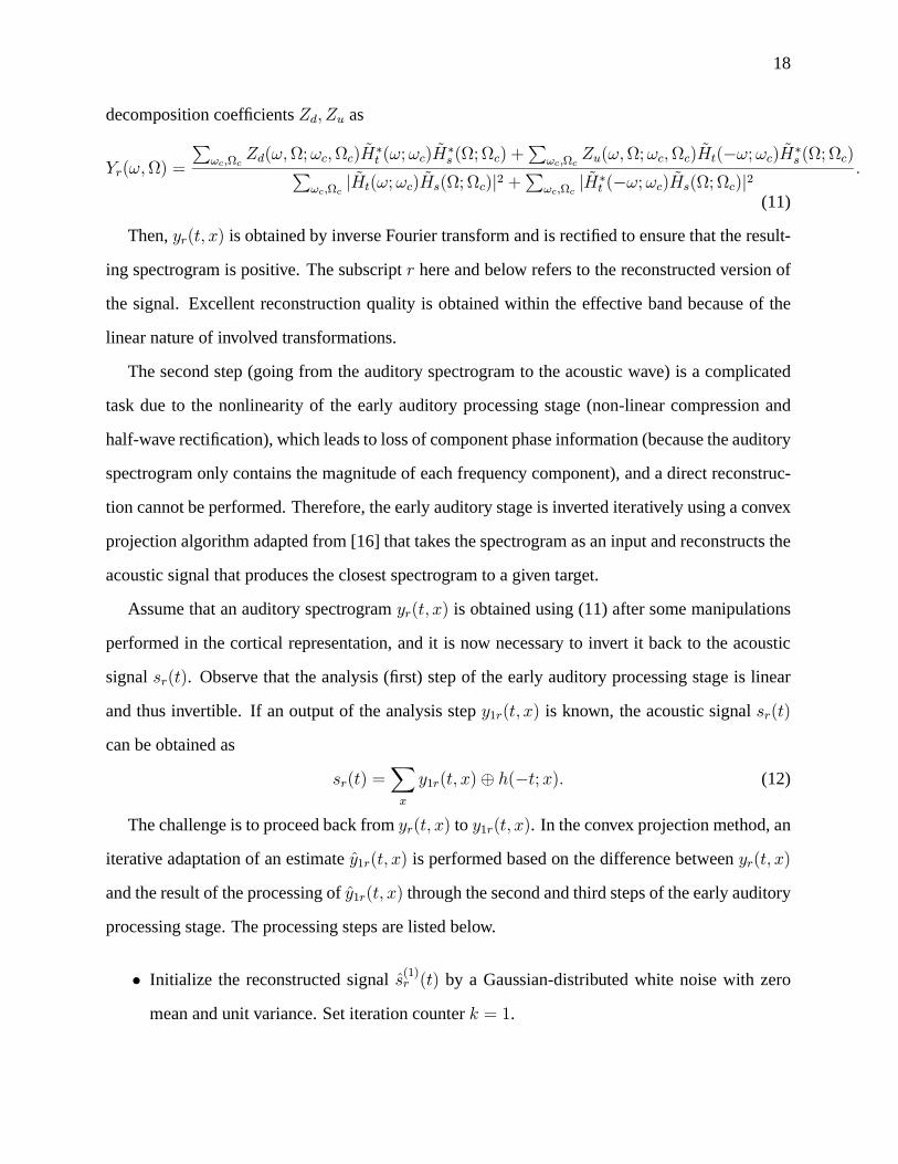
decomposition coefficients Zd, Zu as

Yr(ω,Ω) =

Pωc,Ωc

Zd(ω,Ω;ωc,Ωc)H∗t (ω;ωc)H

∗s (Ω;Ωc) +

Pωc,Ωc

Zu(ω,Ω;ωc,Ωc)Ht(−ω;ωc)H∗s (Ω;Ωc)P

ωc,Ωc|Ht(ω;ωc)Hs(Ω;Ωc)|2 +

Pωc,Ωc

|H∗t (−ω;ωc)Hs(Ω;Ωc)|2

.

(11)

Then, yr(t, x) is obtained by inverse Fourier transform and is rectified to ensure that the result-

ing spectrogram is positive. The subscript r here and below refers to the reconstructed version of

the signal. Excellent reconstruction quality is obtained within the effective band because of the

linear nature of involved transformations.

The second step (going from the auditory spectrogram to the acoustic wave) is a complicated

task due to the nonlinearity of the early auditory processing stage (non-linear compression and

half-wave rectification), which leads to loss of component phase information (because the auditory

spectrogram only contains the magnitude of each frequency component), and a direct reconstruc-

tion cannot be performed. Therefore, the early auditory stage is inverted iteratively using a convex

projection algorithm adapted from [16] that takes the spectrogram as an input and reconstructs the

acoustic signal that produces the closest spectrogram to a given target.

Assume that an auditory spectrogram yr(t, x) is obtained using (11) after some manipulations

performed in the cortical representation, and it is now necessary to invert it back to the acoustic

signal sr(t). Observe that the analysis (first) step of the early auditory processing stage is linear

and thus invertible. If an output of the analysis step y1r(t, x) is known, the acoustic signal sr(t)

can be obtained as

sr(t) =Xx

y1r(t, x)⊕ h(−t; x). (12)

The challenge is to proceed back from yr(t, x) to y1r(t, x). In the convex projection method, an

iterative adaptation of an estimate y1r(t, x) is performed based on the difference between yr(t, x)

and the result of the processing of y1r(t, x) through the second and third steps of the early auditory

processing stage. The processing steps are listed below.

• Initialize the reconstructed signal s(1)r (t) by a Gaussian-distributed white noise with zero

mean and unit variance. Set iteration counter k = 1.

19

• Compute y(k)1r (t, x), y(k)2r (t, x), and y(k)r (t, x) from sr(t) using (1).

• Compute the ratio r(k)(t, x) = yr(t, x)/y(k)r (t, x).

• Adjust y(k+1)1r (t, x) = r(k)(t, x)y(k)1r (t, x).

• Compute s(k+1)r using equation (12).

• Repeat from step 2 unless the preset number of iterations is reached or a certain quality

criterion is met (e.g., the ratio r(k)(t, x) is sufficiently close to unity everywhere).

Sample auditory spectrograms of the original and the reconstructed signals are shown later, and

the reconstruction quality for the speech signal after a sufficient number of iterations is very good.

V. ALTERNATIVE IMPLEMENTATION OF THE EARLY AUDITORY PROCESSING STAGE

An alternative, much faster implementation of the early auditory processing stage (which we

will refer to as a log-Fourier transform early stage) was developed and can best be used for a fixed-

pitch signal (e.g., a musical instrument tone). In this implementation, a simple Fourier transform is

used in place of the processing described by (1). Let us take a short segment of the waveform s(t)

at some time t(j) and perform a Fourier transform of it to obtain S(f). The S(f) is obviously dis-

crete with the total of L/2 points on the linear frequency axis, where L is the length of the Fourier

transform buffer. Some mapping must be established from the points on the linear frequency axis

f to the logarithmically-growing tonotopical axis x. We divide a tonotopical axis into segments

corresponding to channels. Assume that the cochlear filterbank has N channels per octave and

the lowest frequency of interest is f0. Then, the low x(i)l and the high x(i)h ith segment frequency

boundaries are set to be

x(i)l = f02

iN , x

(i)h = f02

i+1N . (13)

S(f) is then remapped onto the tonotopical axis. A point f on a linear frequency axis is said

to fall into the ith segment on the tonotopical axis if x(i)l < f ≤ x(i)h . The number of points that

fall into a segment obviously depends on the segment length, which becomes bigger for higher

20

frequencies (therefore the Fourier transform of s(t) must be performed with very high resolution

and s(t) padded appropriately to ensure that at least a few points on the f axis fall onto the shortest

segment on x axis). Spectral magnitudes are then averaged for all points on the f axis that fall into

the same segment i:

yalt(t(j), x(i)) =

1

B(i)

Xx(i)l <f≤x(i)h

|S(f)|, (14)

where B(i) is the total number of points on f axis that fall into ith segment on x axis (the num-

ber of terms in the summation), and the averaging is performed for all i, generating a time slice

yalt(t(j), x). The process is then repeated for the next time segment of s(t) and so on, and the

results are patched together on time axis to produce yalt(t, x), which can be substituted for the

y(t, x) computed using (1) for all further processing.

The reconstruction proceeds in an inverse manner. At every time slice t(j), a set of y(t(j), x) is

remapped to the magnitude-spectrum S(f) on a linear frequency axis f so that for each frequency

S(f) =

y(t(j), x(i)) if for some i x(i)l < f ≤ x(i)h ,0 otherwise.

(15)

At this point, the magnitude information is set correctly in S(f) to perform inverse Fourier

transform but the phase information is lost. Direct one-step reconstruction from S(f) is much

faster than the iterative convex projection method described above but produces unacceptable re-

sults with clicks and strong interfering noise at the frequency corresponding to the processing

window length. Heavily overlapping window techniques with gradual fade-in and fade-out win-

dowing functions improve the results somewhat but the reconstruction quality is still significantly

below the quality achieved using the iterative projection algorithm described in section 4.

One way to recover the phase information and use one-step reconstruction of s(t) from

magnitude-spectrum S(f) is to store away the bin phases of the forward-pass Fourier transform

and later impose them on S(f) after it is reconstructed from the (altered) cortical representation.

Significantly better continuity of the signal is obtained in this manner. However, it seems that

the stored phases carry the imprint of the original pitch of the signal, which produces undesirable

effects if the processing goal is to perform a pitch shift.

21

However, the negative effect of the phase set carrying the pitch imprint can be reversed and

used for good simply by generating the phase set that corresponds to a desired pitch and imposing

them on S(f). Of course it requires knowledge of the signal pitch, which is not always easy

to obtain. We have used this technique in performing timbre-preserving pitch shift of musical

instrument notes where the exact original pitch F0 (and therefore the exact shifted pitch F 00) is

known. To obtain the set of phases corresponding to the pitch F 00, we generate, in the time domain,

a pulse train of frequency F 00 and take its Fourier transform with the same window length as used

in the processing of S(f). The bin phases of the Fourier transform of the pulse train are then

imposed on the magnitude-spectrum S(f) obtained in (15). In this manner, very good results

are obtained in reconstructing musical tones of a fixed frequency; it should be noted that such

reconstruction is not handled well by iterative convex projection method described above – the

reconstructed signal is not a pure tone but rather constantly jitters up and down, preventing any

musical perception, presumably because the time slices of s(t) are treated independently by convex

projection algorithm, which does not attempt to match signal features from adjacent time frames.

Nevertheless, speech reconstruction is handled better by the significantly slower convex projec-

tion algorithm, because it is not clear how to select F 00 to generate the phase set. If the log-Fourier

transform early stage can be applied to the speech signals, significant processing speed-up can be

achieved. A promising idea is to employ a pitch detection mechanism at each frame of s(t) to

detect F0, to compute F 00 and to impose F 00-consistent phases on S(f) to enable one-step recovery

of s(t), which is the subject of ongoing work.

VI. RECONSTRUCTION QUALITY

It is important to do an objective evaluation of the reconstructed sound quality. The second

(central) stage of the algorithm is perfectly invertible because of the linear nature of the wavelet

transformations involved, and it is the first (early) stage that presents difficulties for the inversion

because of the phase information loss in the processing. Given the modified auditory spectrogram

yr(t, x), the convex projection algorithm described above tries to synthesize the intermediate result

22

y1r(t, x) that, when processed through two remaining steps of the early auditory stage, would

yield yr(t, x) that is as close as possible to yr(t, x). The waveform sr(t) can then be directly

reconstructed from y1r(t, x). The error measure E is the average relative magnitude difference

between the target and the candidate:

E =1

B

Xi,j

|yr(t(j), x(i))− yr(t(j), x(i))|yr(t(j), x(i))

, (16)

where B is the total number of summation terms. During the iterative synthesis of y1r(t, x), the

error E does not drop monotonically; instead, the lower the error, the higher the chance that the

next iteration actually increases the error, in which case the iteration results should be discarded

and a new iteration should be started from the best previously found y1r(t, x).

In practical tests, it was found that the error drops quickly to units of percents and any further

improvement requires very significant computational expense. For the purposes of illustration,

we took the 1200 ms auditory spectrogram of Figure 2 and inverted it back to the waveform

without any modifications. It takes about 2 seconds to execute an iteration of the convex projection

algorithm on a 1.7 GHz Pentium computer. In this sample run, the error after 20, 200 and 2000

iterations was found to be 4.73%, 1.60% and 1.08%, respectively, which is representative of the

general behavior observed in many experiments.

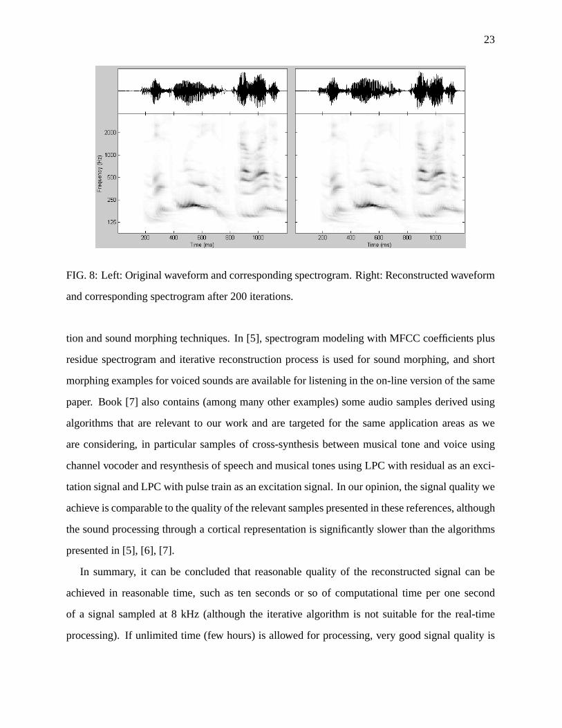
In Figure 8, we plot, side by side, the original auditory spectrogram yr(t, x) from Figure 2

and the result of the reconstruction yr(t, x) after 200 iterations, together with the original and

the reconstructed waveforms. It can be seen that the spectrograms are matched very well, but

the fine structure of the waveform is different, with noticeably less periodicity in some segments.

However, it can be argued that because the original and the reconstructed waveforms produce the

same results when processed through the early auditory processing stage, the perception of these

should be nearly identical, which is indeed the case when the sounds are played to the human ear.

Slight distortions are heard in the reconstructed waveform, but the sound is clear and intelligible.

Increasing the number of iterations further decreases distortions; when the error drops to about

0.5% (tens of thousands of iterations), the signal is almost indistinguishable from the original.

We also compared the quality of the reconstructed signal with the existing pitch modifica-

23

FIG. 8: Left: Original waveform and corresponding spectrogram. Right: Reconstructed waveform

and corresponding spectrogram after 200 iterations.

tion and sound morphing techniques. In [5], spectrogram modeling with MFCC coefficients plus

residue spectrogram and iterative reconstruction process is used for sound morphing, and short

morphing examples for voiced sounds are available for listening in the on-line version of the same

paper. Book [7] also contains (among many other examples) some audio samples derived using

algorithms that are relevant to our work and are targeted for the same application areas as we

are considering, in particular samples of cross-synthesis between musical tone and voice using

channel vocoder and resynthesis of speech and musical tones using LPC with residual as an exci-

tation signal and LPC with pulse train as an excitation signal. In our opinion, the signal quality we

achieve is comparable to the quality of the relevant samples presented in these references, although

the sound processing through a cortical representation is significantly slower than the algorithms

presented in [5], [6], [7].

In summary, it can be concluded that reasonable quality of the reconstructed signal can be

achieved in reasonable time, such as ten seconds or so of computational time per one second

of a signal sampled at 8 kHz (although the iterative algorithm is not suitable for the real-time

processing). If unlimited time (few hours) is allowed for processing, very good signal quality is

24

achieved. The possibility of iterative signal reconstruction in real time is an open question and

work in this area is continuing.

VII. TIMBRE-PRESERVING PITCH MANIPULATIONS

For speech and musical instruments, timbre is conveyed by the spectral envelope, whereas

pitch is mostly conveyed by the harmonic structure, or harmonic peaks. This biologically based

analysis is in the spirit of the cepstral analysis used in speech [25], except that the Fourier-like

transformation in the auditory system is carried out in a local fashion using kernels of different

scales. The cortical decomposition is expressed in the complex domain, with the magnitude being

the measure of the local bandwidth of the spectrum, and the phase being the local symmetry at

each bandwidth. Finally, just as with cepstral coefficients, the spectral envelope varies slowly.

In contrast, the harmonic peaks are only visible at high resolution. Consequently, timbre and

pitch occupy different regions in the multiscale representation. If X is the auditory spectrum of

a given data frame, with length N equal to the number of filters in the cochlear filterbank, and

the decomposition is performed over M scales, then the matrix S of scale decomposition has M

rows, one per scale value, and N columns. If the 1st (top) row of S contains the decomposition

over the finest scale and the M th (bottom) row is the coarsest one, then the components of S in

the upper left triangle (above the main diagonal) can be associated with pitch, whereas the rest

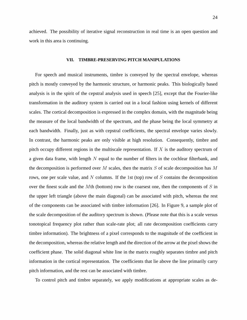
of the components can be associated with timbre information [26]. In Figure 9, a sample plot of

the scale decomposition of the auditory spectrum is shown. (Please note that this is a scale versus

tonotopical frequency plot rather than scale-rate plot; all rate decomposition coefficients carry

timbre information). The brightness of a pixel corresponds to the magnitude of the coefficient in

the decomposition, whereas the relative length and the direction of the arrow at the pixel shows the

coefficient phase. The solid diagonal white line in the matrix roughly separates timbre and pitch

information in the cortical representation. The coefficients that lie above the line primarily carry

pitch information, and the rest can be associated with timbre.

To control pitch and timbre separately, we apply modifications at appropriate scales as de-

25

FIG. 9: Plot of the sample auditory spectrum scale decomposition matrix. The brightness of the

pixel corresponds to the magnitude of the decomposition coefficient, whereas the arrow relative

length and direction at the pixel shows the coefficient phase. Upper triangle of the matrix of

coefficients (above the solid while line) contains information about the pitch of the signal, and the

lower triangle contains information about timbre.

scribed above, and invert the cortical representation back to the spectrogram. Thus, to shift the

pitch while holding the timbre fixed we compute the cortical multiscale representation of the en-

tire sound, shift (along the frequency axis) the triangular part of every time-slice of the hypercube

that holds the pitch information while keeping timbre information intact, and invert the result. To

modify the timbre keeping the pitch intact we do the opposite. It is also possible to splice in pitch

and timbre information from two speakers, or from a speaker and a musical instrument. The result

after inversion back to a sound is a “musical” voice that sings the utterance (or a “talking” musical

instrument).

26

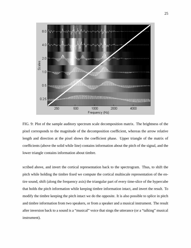
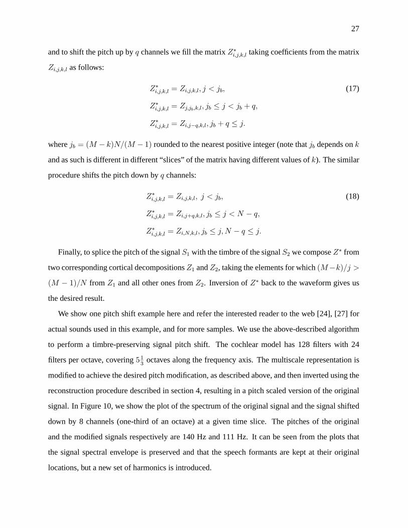
FIG. 10: Spectrum of a speech signal before and after pitch shift. Note that the spectral envelope

is filled with new set of harmonics.

Let us express the timbre-preserving pitch shift algorithm in mathematical terms. The cortical

decomposition results in a set of complex coefficients zu(t, x;ωc,Ωc) and zd(t, x;ωc,Ωc). In the

actual decomposition, the values of t, x,ωc and Ωc are discrete, and the result of the cortical de-

composition is a four-dimensional cube of complex coefficients Zi,j,k,l; let us agree that the first

index i corresponds to the time axis, the second index j corresponds to the frequency axis, the third

index k corresponds to the scale axis, and the fourth index l corresponds to the rate axis. Index j

varies from 1 to N where N is the number of filters in the cochlear filterbank, index k varies from

1 to M (in order of scale increase) where M is the number of scales, and, finally, index l varies

from 1 to 2L where L is the number of rates (zd and zu are juxtaposed in Zi,j,k,l matrix as pictured

on the horizontal axis in Figure 7: l = 1 corresponds to zd with the highest rate, l = 2 to zd with

the next lower rate, l = L to zd with the lowest rate, l = L+1 to zu with the lowest rate, l = L+2

to zu with the next higher rate, and l = 2L to zu with the highest rate; this particular order is

unimportant for pitch modifications described below anyway). Then, the coefficient is assumed to

carry pitch information if it lies above the diagonal in Figure 9 (i.e., if (M − k)/j > (M − 1)/N),

27

and to shift the pitch up by q channels we fill the matrix Z∗i,j,k,l taking coefficients from the matrix

Zi,j,k,l as follows:

Z∗i,j,k,l = Zi,j,k,l, j < jb, (17)

Z∗i,j,k,l = Zj,jb,k,l, jb ≤ j < jb + q,

Z∗i,j,k,l = Zi,j−q,k,l, jb + q ≤ j.

where jb = (M − k)N/(M − 1) rounded to the nearest positive integer (note that jb depends on k

and as such is different in different “slices” of the matrix having different values of k). The similar

procedure shifts the pitch down by q channels:

Z∗i,j,k,l = Zi,j,k,l, j < jb, (18)

Z∗i,j,k,l = Zi,j+q,k,l, jb ≤ j < N − q,

Z∗i,j,k,l = Zi,N,k,l, jb ≤ j,N − q ≤ j.

Finally, to splice the pitch of the signal S1 with the timbre of the signal S2 we compose Z∗ from

two corresponding cortical decompositionsZ1 and Z2, taking the elements for which (M−k)/j >(M − 1)/N from Z1 and all other ones from Z2. Inversion of Z∗ back to the waveform gives us

the desired result.

We show one pitch shift example here and refer the interested reader to the web [24], [27] for

actual sounds used in this example, and for more samples. We use the above-described algorithm

to perform a timbre-preserving signal pitch shift. The cochlear model has 128 filters with 24

filters per octave, covering 513

octaves along the frequency axis. The multiscale representation is

modified to achieve the desired pitch modification, as described above, and then inverted using the

reconstruction procedure described in section 4, resulting in a pitch scaled version of the original

signal. In Figure 10, we show the plot of the spectrum of the original signal and the signal shifted

down by 8 channels (one-third of an octave) at a given time slice. The pitches of the original

and the modified signals respectively are 140 Hz and 111 Hz. It can be seen from the plots that

the signal spectral envelope is preserved and that the speech formants are kept at their original

locations, but a new set of harmonics is introduced.

28

The algorithm is sufficiently fast to be performed in real-time if used with log-Fourier transform

early stage (described in section 5) in place of a cochlear filterbank to eliminate the need for an it-

erative inversion process. Additionally, in this particular application it is not necessary to compute

the full cortical representation of the sound. It is enough to perform only scale decomposition for

every time frame of the auditory spectrogram because shifts are done along the frequency axis and

can be performed in each time slice of the hypercube independently; thus, the rate decomposition

is unnecessary. We have used the algorithm in a small-scale study in an attempt to generate maxi-

mally separable sounds to improve simultaneous eligibility of multiple competing messages [21];

it was found that the pitch separation does improve the perceptual separability of sounds and the

recognition rate. Also, we have used the algorithm to shift a pitch of a sound sample and thus to

synthesize different notes of a newly created musical instrument that has the timbre characteristics

of two existing instruments. This application is described in more details in the following section.

VIII. TIMBRE MANIPULATIONS

Timbre is captured in the multiscale representation both by the spectral envelope and by the sig-

nal dynamics. Spectral envelope variations or replacements can be done by modifying the lower

right triangle in the multiscale representation of the auditory spectrum, while sound dynamics is

captured by the rate decomposition. Selective modifications to enhance or diminish the contri-

butions of components of a certain rate can change the dynamic properties of the sound. As an

illustration, and as an example of information separation across the cells of different rates, we

synthesize a few sound samples using simple modifications to make the sound either abrupt or

slurred. One such simple modification is to zero out the cortical representation decomposition co-

efficients that correspond to the “fast” cells, creating the impression of a low-intelligibility sound

in an extremely reverberant environment; the other one is to remove “slow” cells, obtaining an

abrupt sound in an anechoic environment (see [24], [27] for the actual sound samples where the

decomposition was performed over the rates of 2, 4, 8 and 16 Hz; from these, “slow” rates are

2 and 4 Hz and “fast” rates are 8 and 16 Hz). It might be possible to use such modifications in

29

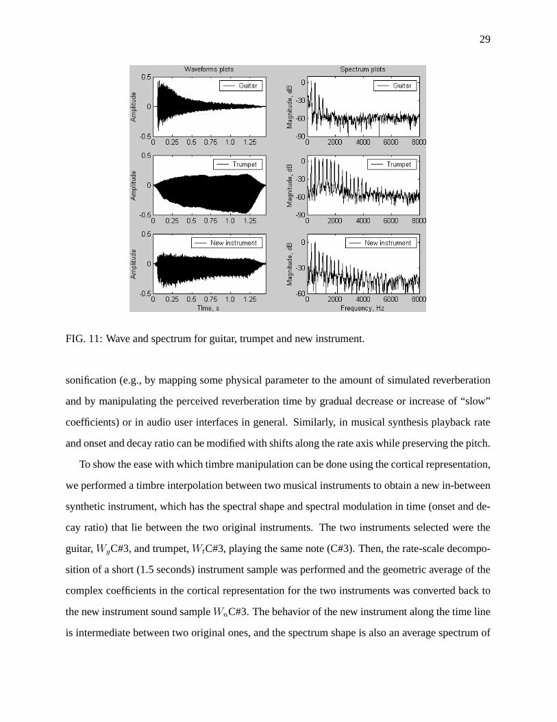
FIG. 11: Wave and spectrum for guitar, trumpet and new instrument.

sonification (e.g., by mapping some physical parameter to the amount of simulated reverberation

and by manipulating the perceived reverberation time by gradual decrease or increase of “slow”

coefficients) or in audio user interfaces in general. Similarly, in musical synthesis playback rate

and onset and decay ratio can be modified with shifts along the rate axis while preserving the pitch.

To show the ease with which timbre manipulation can be done using the cortical representation,

we performed a timbre interpolation between two musical instruments to obtain a new in-between

synthetic instrument, which has the spectral shape and spectral modulation in time (onset and de-

cay ratio) that lie between the two original instruments. The two instruments selected were the

guitar,WgC#3, and trumpet,WtC#3, playing the same note (C#3). Then, the rate-scale decompo-

sition of a short (1.5 seconds) instrument sample was performed and the geometric average of the

complex coefficients in the cortical representation for the two instruments was converted back to

the new instrument sound sampleWnC#3. The behavior of the new instrument along the time line

is intermediate between two original ones, and the spectrum shape is also an average spectrum of

30

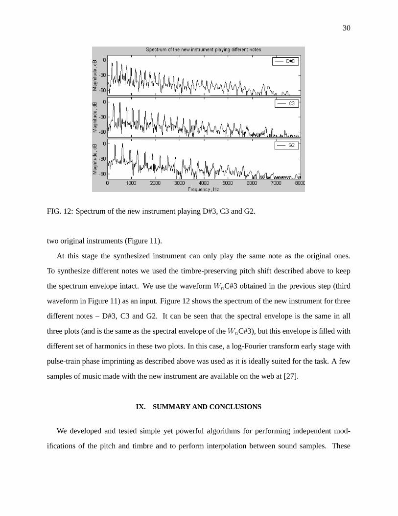
FIG. 12: Spectrum of the new instrument playing D#3, C3 and G2.

two original instruments (Figure 11).

At this stage the synthesized instrument can only play the same note as the original ones.

To synthesize different notes we used the timbre-preserving pitch shift described above to keep

the spectrum envelope intact. We use the waveform WnC#3 obtained in the previous step (third

waveform in Figure 11) as an input. Figure 12 shows the spectrum of the new instrument for three

different notes – D#3, C3 and G2. It can be seen that the spectral envelope is the same in all

three plots (and is the same as the spectral envelope of theWnC#3), but this envelope is filled with

different set of harmonics in these two plots. In this case, a log-Fourier transform early stage with

pulse-train phase imprinting as described above was used as it is ideally suited for the task. A few

samples of music made with the new instrument are available on the web at [27].

IX. SUMMARY AND CONCLUSIONS

We developed and tested simple yet powerful algorithms for performing independent mod-

ifications of the pitch and timbre and to perform interpolation between sound samples. These

31

algorithms are a new application of the cortical representation of the sound [3], which extracts the

perceptually important features similarly to the processing believed to occur in auditory pathways

in primates, and thus can be used for making sound modifications tuned for and targeted to the

ways the human nervous system processes information. We obtained promising results and are

using these algorithms in ongoing development of auditory user interfaces.

ACKNOWLEDGMENTS

Partial support of ONR grant N000140110571 and NSF award 0205271 is gratefully acknowl-

edged.

REFERENCES

[1] D. N. Zotkin, S. A. Shamma, P. Ru, R. Duraiswami, L. S. Davis (2003). “Pitch and timbre

manipulations using cortical representation of sound”, Proc. ICASSP 2003, Hong Kong,

April 2003, vol. 5, pp. 517-520. (Reprinted in Proc. ICME 2003, Baltimore, MD, July 2003,

vol. 3, pp. 381-384, because of the cancellation of ICASSP 2003 conference meeting).

[2] M. Elhilali, T. Chi, and S. A. Shamma (2002). “A spectro-temporal modulation index for

assessment of speech intelligibility”, Speech Communications, in press.

[3] T. Chi, P. Ru, and S. A. Shamma (2004). “Multiresolution spectrotemporal analysis of com-

plex sounds”, submitted to Speech Communications.

[4] T. Chi, Y. Gao, M. C. Guyton, P. Ru, and S. A. Shamma (1999). “Spectro-temporal modula-

tion transfer functions and speech intelligibility”, J. Acoust. Soc. Am., vol. 106.

[5] M. Slaney, M. Covell and B. Lassiter (1996). “Automatic audio morphing”, Proc. IEEE

ICASSP 1996, Atlanta, GA.

[6] X. Serra (1997). “Musical sound modeling with sinusoids plus noise”, in Musical Signal

Processing, ed. by C. Roads et al., Swets & Zeitlinger Publishers, Lisse, The Netherlands.

32

[7] P. R. Cook (2002). “Real Sound Synthesis for Interactive Applications”, A. K. Peters Ltd.,

Natick, MA.

[8] S. Barass (1996). “Sculpting a sound space with information properties: Organized sound”,

Cambridge University Press.

[9] http://www.icad.org/

[10] G. Kramer et al (1997). “Sonification report: Status of the field and research agenda”,

Prepared for NSF by members of the ICAD. (Available on the World Wide Web at

http://www.icad.org/websiteV2.0/References/nsf.html).

[11] S. Bly (1994). “Multivariate data mapping”, in Auditory display: Sonification, audification

and auditory interfaces, G. Kramer, ed. Santa Fe Institute Studies in the Sciences of Com-

plexity, Proc. Vol. XVIII, pp. 405-416, Addison Wesley, Reading, MA.

[12] D. Zotkin, R. Duraiswami, and L. Davis (2002). “Rendering localized spatial audio in a

virtual auditory space”, IEEE Transactions on Multimedia, vol. 6(4), 2004, pp. 553-564.

[13] D. S. Brungart (2001). “Informational and energetic masking effects in the perception of two

simultaneous talkers”, J. Acoust. Soc. Am., vol. 109, pp. 1101-1109.

[14] C. J. Darwin and R. W. Hukin (2000). “Effects of reverberation on spatial, prosodic, and

vocal-tract size cues to selective attention”, J. Acoust. Soc. Am., vol. 108, pp. 335-342.

[15] C. J. Darwin and R. W. Hukin (2000). “Effectiveness of spatial cues, prosody, and talker

characteristics in selective attention”, J. Acoust. Soc. Am., vol. 107, pp. 970-977.

[16] X. Yang, K. Wang, and S. A. Shamma (1992). “Auditory representation of acoustic signals”,

IEEE Transactions on Information Theory, vol. 38, no. 2, pp. 824-839.

[17] M. L. Hawley, R. Y. Litovsky, and H. S. Colburn (1999). “Speech intelligibility and localiza-

tion in multi-source environments”, J. Acoust. Soc. Am., vol. 105, pp. 3436-3448.

[18] W. A. Yost, R. H. Dye, and S. Sheft (1996). “A simulated cocktail party effect with up to

three sound sources”, Perception and Psychophysics, vol. 58, pp. 1026-1036.

[19] B. Arons (1992). “A review of the cocktail party effect”, J. Am. Voice I/O Society, vol. 12.

[20] P. F. Assman (1999). “Fundamental frequency and the intelligibility of competing voices”,

Proc. 14th International Conference of Phonetic Sciences, pp. 179-182.

33

[21] N. Mesgarani, S. A. Shamma, K. W. Grant, and R. Duraiswami (2003). “Augmented intel-

ligibility in simultaneous multi-talker environments”, Proc. ICAD 2003, Boston, MA, pp.

71-74.

[22] A. S. Bregman (1991). “Auditory scene analysis: The perceptual organization of sound”,

MIT Press, Cambridge, MA.

[23] N. Kowalski, D. Depireux, and S. A. Shamma (1996). “Analysis of dynamic spectra in ferret

primary auditory cortex: Characteristics of single unit responses to moving ripple spectra”,

J. Neurophysiology, vol. 76(5).

[24] http://www.isr.umd.edu/CAAR/

[25] F. Jelinek (1998). “Statistical Methods for Speech Recognition”, MIT Press, Cambridge,

MA.

[26] R. Lyon and S. A. Shamma (1996). “Auditory representations of timbre and pitch”, in Audi-

tory Computations, volume 6 of Springer Handbook of Auditory Research, Springer-Verlag

New York Inc, pp. 221-270.

[27] http://dz.msk.ru/ICASSP2003/