NEUROFUZZY MODEL BASED PREDICTIVECONTROL OF WELD FUSION ZONE GEOMETRY

Y. M. Zhang, Senior Member, IEEE and R. Kovacevic*

Abstract. A closed-loop system is developed to control the weld fusion which is specified by the top-

side and back-side bead widths of the weld pool. Because in many applications only a top-side sensor

is allowed which is attached to and moves with the welding torch, an image processing algorithm and

neurofuzzy model have been incorporated to measure and estimate the top-side and back-side bead

widths based on an advanced top-side vision sensor. The welding current and speed are selected as

the control variables. It is found that the correlation between any output and input depends on the value

of another input. This cross-coupling implies that a non-linearity exists in the process being controlled.

A neurofuzzy model is used to model this non-linear dynamic process. Based on the dynamic fuzzy

model, a predictive control system has been developed to control the welding process. Experiments

confirmed that the developed control system is effective in achieving the desired fusion state despite the

different disturbances.

Key words: predictive control, fuzzy control, modeling, welding.

Y. M. Zhang is with the Welding Research and Development Laboratory, Center for Robotics and ManufacturingSystems, University of Kentucky, Lexington, KY 40506.

R. Kovacevic is presently with the Department of Mechanical Engineering, Southern Methodist University, Dallas,TX 75275.

This work is supported by the National Science Foundation (DMI-9634735), Allison Engine Company, Indianapolis,IN and the Center for Robotics and Manufacturing Systems.

2

1. INTRODUCTION

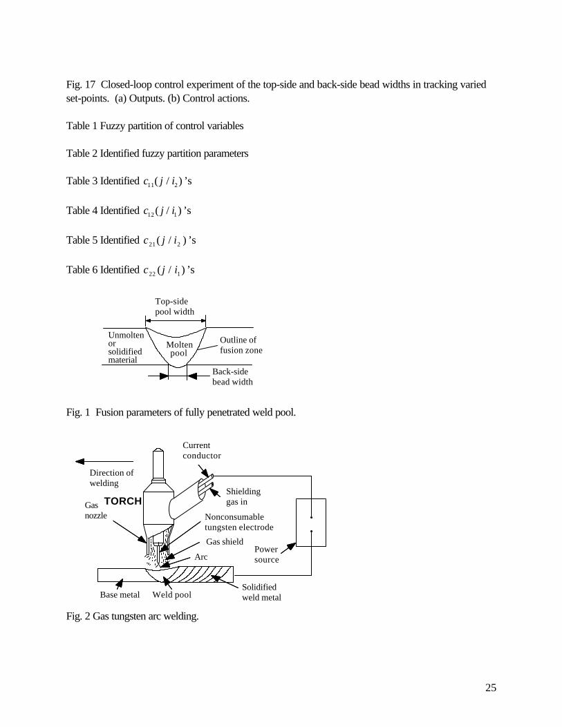
Fusion is the primary requirement of a welding operation. The fusion state can be specified using the

outline of the cross-sectional solidified weld bead (Fig. 1). Extraction and control of the fusion outline is

evidently impractical. A few geometrical parameters should be used to characterize the fusion zone and

then be controlled to achieve the desired fusion.

This study focuses on controlling the fusion state of fully penetrated welds in gas tungsten arc (GTA)

welding. The fusion state on a cross section is characterized using two parameters of the fusion zone,

the top-side and back-side widths of the fusion zone (Fig. 1). Therefore, the top-side width w and

back-side bead width wb of the weld pool are referred to as the fusion state. A multivariable system

will be developed to control w and wb in this study.

Pool width control has been extensively studied. One of the pioneering works was done by Vroman

and Brandt [1] who used a line scanner to detect the weld pool region. Chin et al. found that the slope

of the infrared intensity becomes zero when the liquid-solid interface of the weld pool is crossed [2, 3].

This zero slope is caused by the emissivity difference between the liquid and solid [2]. In order to

directly observe the weld pool, the intensive arc light should be avoided or eliminated. Richardson et al.

proposed the co-axial observation to avoid the arc light [4]. Pietrzak and Packer have developed a

weld pool width control system based on the co-axial observation [5].

Compared with the pool width, weld penetration is a more critical component of the weld quality.

For the case of full penetration, the state of the weld penetration is specified by the back-side bead

width wb (Fig. 1). With a back-side sensor, wb can be reliably measured. However, it is often

required that the sensor be attached to and move with the torch to form a so-called top-side sensor.

3

For such a sensor, wb is invisible. Hence, extensive studies have been done to explore the possibility of

indirectly measuring wb based on pool oscillation, infrared radiation, ultrasound, and radiography.

Although many valuable results have been achieved, only a few control systems are available to

quantitatively estimate and control the back-side bead width.

Fusion control requires the simultaneous control of both the top-side and back-side bead widths,

and is therefore more complicated than either penetration or pool width control. Hardt et al. have

simultaneously controlled the depth, which specifies the weld penetration state for the case of partial

penetration, and width of the weld pool using top-side and back-side sensors [6]. To obtain a top-side

sensor based control system, we have proposed estimating the back-side bead width using the sag

geometry behind the weld pool [7]. Based on a detailed dynamic modeling study [8], an adaptive

system has been developed to control both the top-side and back-side widths of the weld pool [9]. In

this case, a delay arises since the feedback can only be measured at the already solidified sag behind the

pool.

More instantaneous and accurate information can be acquired from the weld pool. In order to use

the weld pool information in welding process control, a real-time image processing algorithm was

developed to detect the weld pool boundary in a previous study [10] from the images captured by a

high shutter speed camera assisted with a pulsed laser [11]. Hence, the weld pool geometry can be

utilized to develop more advanced welding process control systems.

It is known that skilled operators can estimate and control the welding process based on pool

observation. This implies that an advanced control system could be developed to control the fusion

state by emulating the estimation and decision making processes of human operators. In the past,

operator’s experience was the major source to establish the fuzzy model that emulates the operator.

4

Recently, neurofuzzy approach, i.e., determining the parameters in fuzzy models using optimization

algorithms developed in neural network training, has been employed to establish fuzzy models based on

experimental data. Hence, we developed a neurofuzzy system for estimating the back-side bead width

from the pool geometry [12]. In this work, a neurofuzzy dynamic model based multivariable system will

be designed to control the fusion state using the top-side pool width and the estimated back-side bead

width as the feedback of the fusion state.

2. PROCESS

2.1 Controlled Process

Gas tungsten arc (GTA) is used for precise joining of metals. The GTA welding process is illustrated

in Fig. 2. A nonconsumable tungsten electrode is held by the torch. Once the arc is established, the

electrical current flows from one terminal of the power supply to another terminal through the electrode,

arc, and workpiece. The temperature of the arc can reach 8000 10500− K [13], and therefore the

workpiece becomes molten, forming the weld pool, whereas the tungsten electrode remains unmolten.

The shielding gas is fed through the torch to protect the electrode, molten weld pool, and solidifying

weld metal from being contaminated by the atmosphere.

The major adjustable welding parameters include the welding current, arc length, and travel speed of

the torch. In general, the weld pool increases as the current increases and the travel speed decreases.

For GTA welding, the welding current is maintained constant by the inner closed-loop control system of

the power supply despite the variations in the arc length and other parameters. Thus, when the arc

length increases, the arc voltage increases so that the arc power increases, but the distribution of the arc

energy is decentralized so that the efficiency of the arc decreases. As a result, the correlation between

the weld pool and arc length may not be straightforward. In addition to these three welding parameters,

5

the weld pool is also determined by the welding conditions such as the heat transfer condition, material,

thickness, and chemical composition of the workpiece, shielding gas, angle of the electrode tip, etc. In a

particular welding process control system, only a few selected welding parameters are adjusted through

the feedback algorithm to compensate for the variations in the welding conditions.

Compared with the arc length, the roles of the welding current and welding speed in determining the

weld pool and weld fusion geometry are much more significant and definite. For many automated

welding systems, the welding speed can be adjusted on-line. Such an on-line adjustment may also be

done for many advanced welding robots with proper interfaces. Thus, in addition to the welding

current, we selected the welding speed as another control variable. The controlled process can

therefore be defined as a GTA welding process in which the welding current and speed are adjusted

on-line to achieve the desired back-side and top-side widths of the weld pool.

2.2 Non-linearity:

The heat input of the arc in a unit interval along the travel direction can be written as

∆H i v u∝ ( / )2 (1)

where i is the welding current, v is the welding speed, and u is the welding voltage. Roughly

speaking, one can assume that the area of the weld pool is approximately proportional to ∆H .

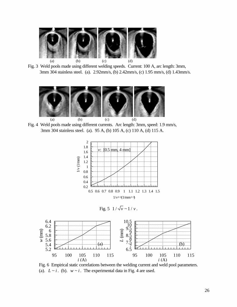
When the welding speed changes, both the length L and width w of the weld pool alter. However,

their ratio w L/ , referred to as the relative width of the weld pool in this work, does not change

significantly (ranged from 0.72 to 0.85 in Fig. 3). This suggests that

L i u v

w i u v

∝

∝

( )( / )

( )( / )

1

1

In our case, the voltage u can be assumed constant. Hence,

6

L f i v

w f i v

∝

∝

1

1

1

1

( )( / )

( )( / ) (2)

where f i i u1 ( ) = .

When the current increases, the relative width w L/ decreases (Fig. 4). This implies:

L f v i

w f v i

c c

c c

∝

∝

( ( ))

( ( ))

2

2

1 1

2 2 (3)

where c1 1> , 0 12< <c , c c1 2 2+ = , and f v u v2 ( ) /= .

During closed-loop control, the control variables i and v are subject to fundamental adjustments so

that f1 and f2 change as the control variables move in the control variable plan i v~ . Hence, the

correlation between the top-side geometrical parameters (width and length) of the weld pool and the

input variables is non-linear. Because of the correlation between the back-side bead width and the top-

side geometrical parameters, it is apparent that the correlation between the back-side bead width and

the control variables is also non-linear. Hence, the controlled plant is a two-input two-output non-linear

multivariable process. Because of the thermal inertia, the process will also be dynamic.

3. NEUROFUZZY NON-LINEAR DYNAMIC MODELING

3.1 Neurofuzzy Modeling:

A fuzzy system has three major conceptual components: rule base, database, and reasoning

mechanism [14]. The rule base consists of the used fuzzy IF-THEN rules. The database contains the

membership functions of the fuzzy sets. The reasoning mechanism performs the inference procedure for

deriving a reasonable output or conclusion based on the IF-THEN rules from the input variables.

In the conventional fuzzy models, the fuzzy linguistic IF-THEN rules are primarily derived from

human experience [15]. Because the fuzzy modeling takes advantage of existing human knowledge

7

which might not be easily or directly utilized by other conventional modeling methods [14], such fuzzy

models have been successfully used in different areas, including manufacturing [16-19]. In these

models, no systematic adjustments are made on the used rules, membership functions, or reasoning

mechanism based on the behavior of the fuzzy model. In general, if the fuzzy rules elicited from the

operators' experience are correct, relevant, and complete [20], the resultant fuzzy model can function

well. However, frequently such fuzzy rules from the operators do not satisfy the correctness, relevance,

and completeness requirements [20]; the rules may be vague and misinterpreted, or the rule base could

be incomplete. In such cases, the performance of the fuzzy system can be greatly improved if

systematic adjustments are made based on its behavior.

The adjustability of the used rules, membership functions, and reasoning mechanism allow the fuzzy

model to adapt to the addressed problem or process. In order to adjust the parameters in the fuzzy

model, various learning techniques developed in the neural network literature have been used. Thus, the

term neurofuzzy modeling is used to refer to the application of algorithms developed through neural

network training to identify parameters for a fuzzy model [14]. A neurofuzzy model can be defined as a

fuzzy model with parameters which can be systematically adjusted using the training algorithms in neural

network literature. In neurofuzzy modeling, the abstract thoughts or concepts in human reasoning are

combined with numerical data so that the development of fuzzy models becomes more systematic and

less time consuming. As a result, neurofuzzy systems have been successfully used in different areas [21-

24].

Most neurofuzzy systems have been developed based on the Sugeno-type fuzzy model [25]. A

typical fuzzy rule in a Sugeno-type model has the form: IF x is A and y is B THEN z f x y= ( , ) .

Here A and B are fuzzy sets, and z f x y= ( , ) is a crisp function which can be any function as long as

8

the system outputs can be appropriately described within the fuzzy region specified by the antecedent of

the rule [14]. In this paper, a neurofuzzy system will be developed to model the non-linear dynamics of

the process being controlled.

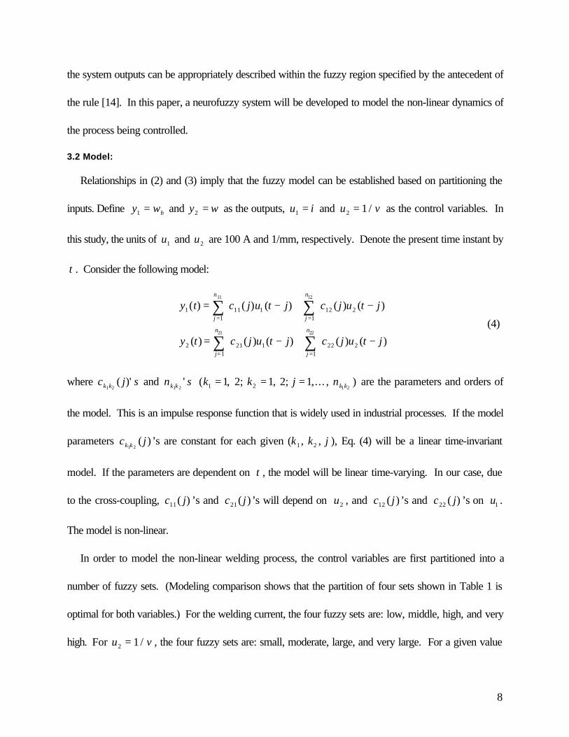
3.2 Model:

Relationships in (2) and (3) imply that the fuzzy model can be established based on partitioning the

inputs. Define y wb1 = and y w2 = as the outputs, u i1 = and u v2 1= / as the control variables. In

this study, the units of u1 and u2 are 100 A and 1/mm, respectively. Denote the present time instant by

t . Consider the following model:

y t c j u t j c j u t j

y t c j u t j c j u t j

j

n

j

n

j

n

j

n

11

11 11

12 2

21

21 11

22 2

11 12

21 22

( ) ( ) ( ) ( ) ( )

( ) ( ) ( ) ( ) ( )

= − + −

= − + −

= =

= =

∑ ∑

∑ ∑ (4)

where c j sk k1 2( )' and n sk k1 2

' ( , , ,... , )k k j nk k1 21 1 11 2

= = = 2; 2; are the parameters and orders of

the model. This is an impulse response function that is widely used in industrial processes. If the model

parameters c jk k1 2( ) ’s are constant for each given (k k1 2, , j ), Eq. (4) will be a linear time-invariant

model. If the parameters are dependent on t , the model will be linear time-varying. In our case, due

to the cross-coupling, c j11( ) ’s and c j21( ) ’s will depend on u2 , and c j12 ( ) ’s and c j22 ( ) ’s on u1 .

The model is non-linear.

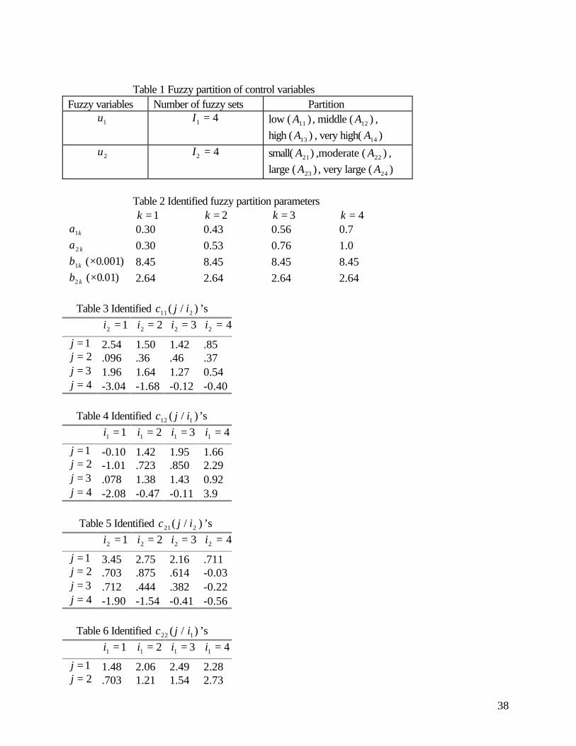
In order to model the non-linear welding process, the control variables are first partitioned into a

number of fuzzy sets. (Modeling comparison shows that the partition of four sets shown in Table 1 is

optimal for both variables.) For the welding current, the four fuzzy sets are: low, middle, high, and very

high. For u v2 1= / , the four fuzzy sets are: small, moderate, large, and very large. For a given value

9

of u j , the degree of truth that u j belongs to its i th fuzzy set is measured by the membership function

Aji :

( )A u u a b i Iji j j ji ji j( ) exp ( ) / ( )= − − ≤ ≤2 1 (5)

where I j is the number of the partitioned fuzzy sets for u j ( , )j = 1 2 , a ji and b ji are the parameters

of the membership function.

Based on the partition of the control variables, the following rules can be applied:

If is then

If is then (6)

u t j A c j c j i

u t j A c j c j ik

i k k

i k k

2 2 1 1 2

1 1 2 2 1

2

1

1 2( ) ( ) ( / )

( ) ( ) ( / )( , )

− =

− =

=

Here c j ik1 2( / ) and c j ik2 1( / ) are constant for the given j i, , 1 and i2 . Also, i2 in c j ik1 2( / ) and

i1 in c j ik2 1( / ) are used to indicate that the parameters c jk1( ) and c jk2 ( ) (in model (4)) depend on

the partition set i2 and i1 that u t j2 ( )− and u t j1( )− belong to, respectively.

Rule (6) is designed to account for the cross-coupling only. Theoretically, based on (2) and (3), the

rule should be:

If u t j1( )− is A i1 1 and u t j2 ( )− is A i2 2

then c j c j i ik k1 1 1 2( ) ( / , )= and c j c j i ik k2 2 1 2( ) ( / , )=

(6A)

However, in our case, the range of the welding speed in the closed-loop control will be 1.0 mm to 3.0

mm. In this range, the correlation between 1 / v and 1 / v can be roughly linear (Fig. 5). Hence, we

can regard L f i v∝ 1 1( )( / ) and w f i v∝ 1 1( )( / ) . Also, from Fig. 4, the static correlations between the

weld pool parameters and the welding current in Fig. 6 can be obtained. Again, although the

correlations are non-linear, the non-linearity is slight. As a result, as will be discussed in Section 5,

experimental data analysis suggests that the above more complex rule (6A) does not significantly

10

improve the modeling. This implies that the cross-coupling is the dominant factor which causes the non-

linearity. Hence, Rule (6) is used.

In our case, the partition is fuzzy. This implies that u t j2 ( )− (or u t j1( )− ) may simultaneously

belong to A21 ,..., and A I2 2(or A11 ,..., and A I1 1

), but with different membership functions. Hence,

c j A u t j c j i k j n

c j A u t j c j i k j n

k ii

I

k k

k ii

I

k k

1 2 21

1 2 1

2 1 11

2 1 2

2

2

2

1

1

1

1 2 1

1 2 1

( ) ( ( )) ( / ) ( , ; , ..., )

( ) ( ( )) ( / ) ( , ; ,..., )

= − = =

= − = =

=

=

∑

∑

(7)

4. IDENTIFICATION ALGORITHM

The identification of a fuzzy model consists of structure identification and parameter estimation.

During identification, the parameters are estimated for different structures. The final structure, i.e., the

fuzzy variable partition in this case, is selected by comparing different models. This is, in general, very

inefficient. Also, the decision is made purely based on statistical (mathematical) analysis. No process

characteristics or designer's experience are involved. If the designer is familiar with the process, an

experience-based partition may be appropriate. Thus, as suggested in [14], we have selected and

partitioned the fuzzy variables based on our understanding of the welding process (Table 1). Hence, the

identification of the fuzzy model is simplified as a parameter estimation problem.

Denote the data as:

{ ( ), ( ), ( ), ( )} ( )u t u t y t y t T t T1 2 1 2 0 1 (8)≤ ≤

and the prediction errors as

δδ

1 1 1

2 2 2

( ): ( ) $ ( )

( ): ( ) $ ( )

t y t y t

t y t y t

= −= −

(9)

11

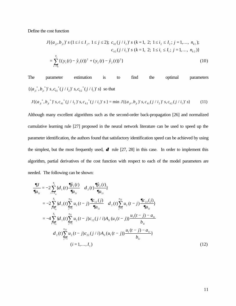
Define the cost function

J a b s i I j c j i s k i I j n

c j i s k i I j n

y t y t y t y t

ji ji j k k

k k

t T

T

{( , )' ( , ); ( / )' ( , ; ,..., );

( / )' ( , ; , ..., )}

{( ( ) $ ( )) ( ( ) $ ( ))

;

;

+ } (10)

1 1 2 1 2 1 1

1 2 1 11 2 2 2 1

2 1 1 1 2

1 12

2 22

0

1

≤ ≤ ≤ ≤ = ≤ ≤ =

= ≤ ≤ =

= − −=∑

The parameter estimation is to find the optimal parameters

{( , )' , ( / )' , ( / )' }* * * *a b s c j i s c j i sji ji k k1 2 2 1 so that

J a b s c j i s c j i s J a b s c j i s c j i sji ji k k ji ji k k{( , )' , ( / )' , ( / )' } min {( , )' , ( / )' , ( / )' }* * * *1 2 2 1 1 2 2 1 (11)=

Although many excellent algorithms such as the second-order back-propagation [26] and normalized

cumulative learning rule [27] proposed in the neural network literature can be used to speed up the

parameter identification, the authors found that satisfactory identification speed can be achieved by using

the simplest, but the most frequently used, δδ rule [27, 28] in this case. In order to implement this

algorithm, partial derivatives of the cost function with respect to each of the model parameters are

needed. The following can be shown:

∂∂

δ∂∂

δ∂∂

δ∂∂

δ∂

∂

δ

Ja

ty t

at

y t

a

t u t jc j

at u t j

c ja

t u t j c j i A u t ju t j a

b

i i it T

T

ij

n

t T

T

ij

n

ii

ij

n

t T

11

1

12

2

1

1 212

112 2

22

11

1 2 12 1 11 1

11

2

2

4

0

1

12

0

1 22

12

0

= − +

= − − + −

= − − −− −

=

== =

==

∑

∑∑ ∑

∑

{ ( )$ ( )

( )$ ( )

}

{ ( ) ( )( )

( ) ( )( )

}

{ ( ) ( ) ( / ) ( ( ))( )

T

ii

ij

n

t u t j c j i A u t ju t j a

b

i I

1

22

2 2 22 1 11 1

11

11

∑

∑+ − −− −

==

) (12)

δ ( ) ( ) ( / ) ( ( ))( )

}

( ,...,

12

∂∂

δ

δ

Ja

t u t j c j i A u t ju t j a

b

t u t j c j i A u t ju t j a

bi I

ii

i

ij

n

t T

T

ii

ij

n

21 1 11 2 2

2 2

21

2 1 21 2 22 2

212

4

1

11

0

1

21

= − − −− −

+ − −− −

=

==

=

∑∑

∑

{ ( ) ( ) ( / ) ( ( ))( )

( ) ( ) ( / ) ( ( ))( )

} ( ,..., ) (13)

∂∂

δ

δ

Jb

t u t j c j i A u t ju t j a

b

t u t j c j i A u t ju t j a

bi I

ii

i

ij

n

t T

T

ii

ij

n

11 2 12 1 1

1 12

12

1

2 2 22 1 11 1

2

12

11

2

1

12

0

1

22

=

) (14)

− − −− −

+ − −− −

=

==

=

∑∑

∑

{ ( ) ( ) ( / ) ( ( ))( ( ) )

( ) ( ) ( / ) ( ( ))( ( ) )

} ( ,... ,

∂∂

δ

δ

Jb

t u t j c j i A u t ju t j a

b

t u t j c j i A u t ju t j a

bi I

ii

i

ij

n

t T

T

ii

ij

n

21 1 11 2 2

2 22

22

1

2 1 21 2 22 2

2

22

12

2

1

11

0

1

21

= − − −− −

+ − −− −

=

==

=

∑∑

∑

{ ( ) ( ) ( / ) ( ( ))( ( ) )

( ) ( ) ( / ) ( ( ))( ( ) )

} ( , ..., ) (15)

∂∂

δ∂

∂δ

∂∂

δ

Jc j i

ty t

c j it u t j

c jc j i

t u t j A u t j k j n i I

kk

k

kt T

T

kk

kt T

T

k it T

T

k

1 2 1 21

1

1 2

1 2 2 1 2 2

2 2

2 1 2 1 1

0

1

0

1

2

0

1

( / )( )

$ ( )( / )

( ) ( )( )

( / )

( ) ( ) ( ( )) ( , ; , ..., ; ,.. ., )

= − = − −

= − − − = = =

= =

=

∑ ∑

∑ (16)

∂∂

δJc j i

t u t j A u t j k j n i Ik

k it T

T

k2 1

2 1 1 2 1 12 1 2 1 11

0

1

( / )( ) ( ) ( ( )) ( , ; ,..., ; , ..., )= − − − = = =

=∑ (17)

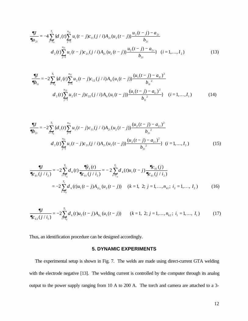
Thus, an identification procedure can be designed accordingly.

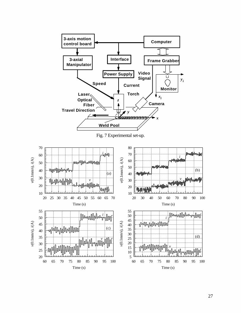
5. DYNAMIC EXPERIMENTS

The experimental setup is shown in Fig. 7. The welds are made using direct-current GTA welding

with the electrode negative [13]. The welding current is controlled by the computer through its analog

output to the power supply ranging from 10 A to 200 A. The torch and camera are attached to a 3-

13

axial manipulator. The motion of the manipulator is controlled by the 3-axis motion control board which

receives the commands from the computer. The motion can be preprogrammed and on-line modified

by the computer in order to achieve the required torch speed and trajectory, including the arc length.

The Control Vision’s ultra-high shutter speed vision system [11] is used to capture the weld pool

images. This system consists of a strobe-illumination unit (pulse laser), camera head and system

controller. The pulse duration of the laser is 3 ns, and the camera is synchronized with the laser pulse.

Thus, the intensity of laser illumination during the pulse duration is much higher than those of the arc and

hot metal. Using this vision system, good weld pool contrast can always be obtained under different

welding conditions. In this study, the camera views the weld pool from the rear at a 45° angle. The

frame grabber digitizes the video signals into 512 512× 8bit digital image matrices. By improving the

algorithm [10] and hardware, the weld pool boundary can now be acquired on-line in 80 ms.

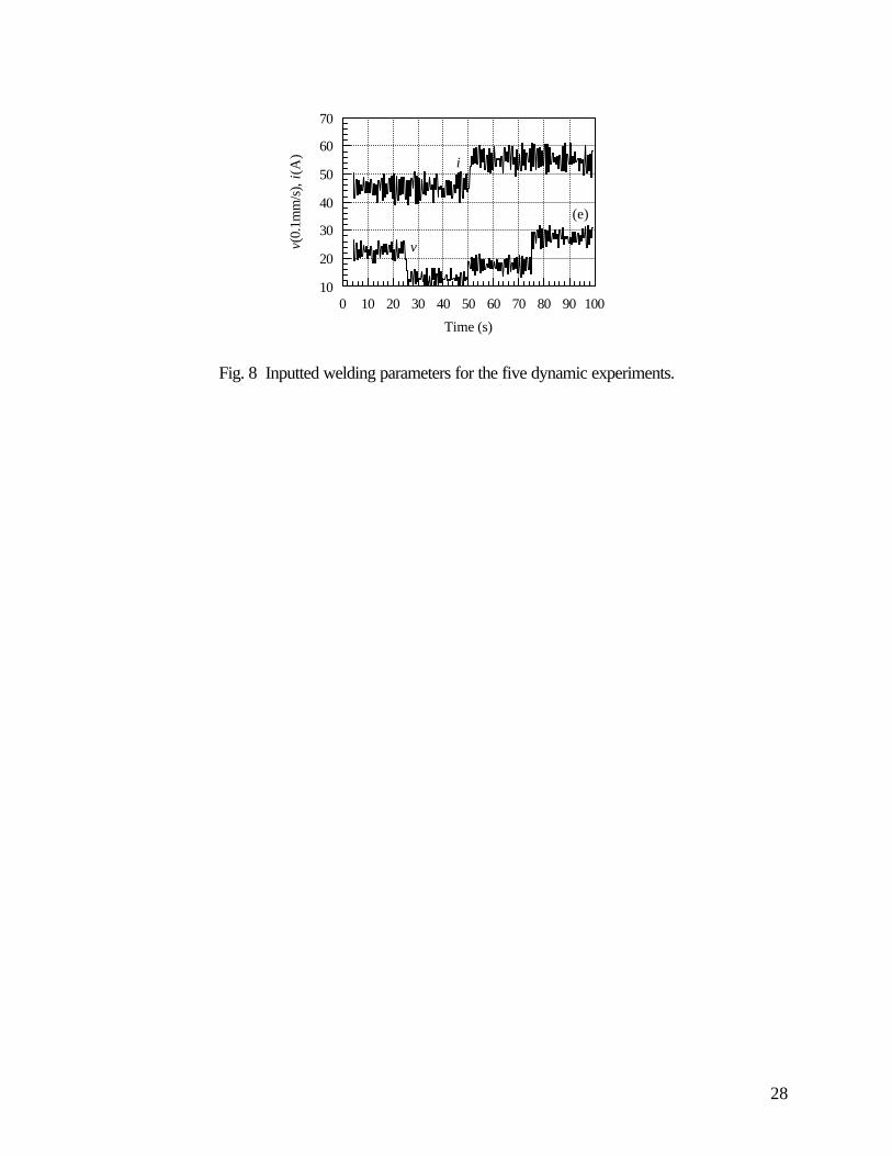
Five experiments have been done on 1 mm thick stainless steel 304 plates. The workpieces are 250

mm in length and 100 mm in width. The shielding gas is pure argon. The arc length is 3 mm in all the

experiments. In order to establish the full penetration mode, the current and welding speed must be in

certain ranges. We have used control variables in larger ranges. Fig. 8 plots the segments in each

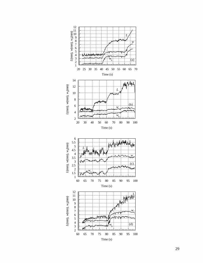
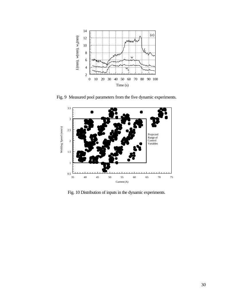
experiment where the inputs have produced fully penetrated weld pools. The measured parameters of

the weld pools in these segments are given in Fig. 9. The back-side bead width can be calculated using

the weld pool parameters and the neurofuzzy model developed in the previous study [12]. The results

have also been illustrated in Fig. 9.

Fig. 10 shows the distribution of the control variables in these segments of experiments. It can be

seen that the welding parameters have filled the projected range of the control variables. This

14

distribution implies that the resultant model can be used during control if the control variables are in the

projected range.

The above experimental data have been used to fit a neurofuzzy model here. It is found that orders

n n n n11 12 21 22 4= = = = are sufficient when the sample period T s= 1 . The identified model

parameters are given in Tables 2-6. Here u t j1( )− and u t j2 ( )− are the average inputs in

(( ) . , ( ) . ],t j T T t j T T− − − +0 5 0 5 rather than at discrete instant t j− .

Assume that τ represents the continuous time, rather than the discrete time instant. The outputs at

τ can be predicted using the inputs in ( . , . ]τ τ− − − +jT T jT T0 5 0 5 ’s ( , ...,max( ,.. ., ))j n n= 1 11 22

no matter whether or not τ / T is an integer. Hence, by applying the identified model, the outputs at

any moment can be predicted.

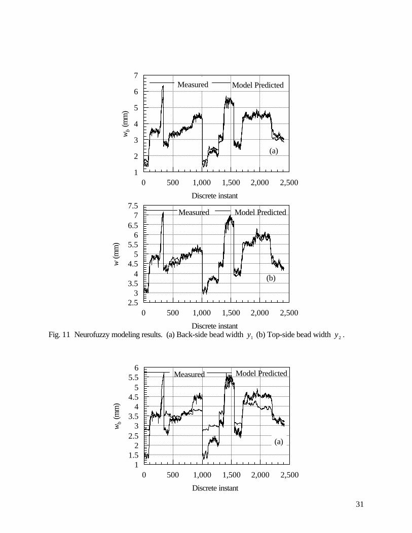
The modeling accuracy of the resultant fuzzy model can be seen in Fig. 11 where the outputs were

measured at 10 Hz. The variances of the fitting errors are 0.039mm 2 and 0.020mm 2 for w and wb ,

respectively. It is found that the no noticed improvement can be made when increasing n sk k1 2' ,

increasing I1 and I2 , or using Rule (6A). In fact, the welding process is subject to uncertainty and its

outputs can not be exactly predicted using the inputs without any errors. The prediction errors in Fig.

11 are certainly not larger than the deviations of the outputs caused by the uncontrollable variations in

the welding process when the same inputs are used. Hence , the obtained model is sufficient.

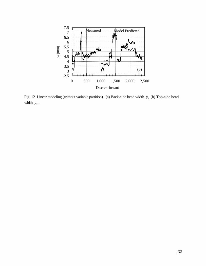
In order to show the effectiveness of the fuzzy model, a linear model has also been fitted. It is found

that the modeling is much poorer (Fig. 12). It is apparent that the used neurofuzzy model structure has

played a critical role in accurately modeling the non-linear dynamics of the process being controlled.

6. FUZZY MODEL BASED PREDICTIVE CONTROL

15

A number of methods could be used to design a neurofuzzy controller [14], including mimicking

another working controller, inverse model, specialized learning, back-propagation through time and

real-time recurrent learning, feedback linearization and sliding control, gain scheduling, etc. The

advantage and limitation of each individual method has been analyzed in [14].

Traditionally, fuzzy controllers have been designed without an explicit model of the process being

controlled. However, in neurofuzzy systems, mathematical models are explicitly used. We notice that

the predictive control principle [29] has recently been incorporated with fuzzy models to provide design

methods for neurofuzzy model based controllers because predictive methods have several advantages

that make them good candidates for industrial applications. Oliveira and Lemos proposed a fuzzy

model based predictive controller for single-input single-output systems [30]. They used relational fuzzy

models, rather than the Sugeno-type models as used in our work. Next, we will develop a predictive

controller for our two-input two-output Sugeno-type model.

At t , the controller needs to determine the control action ( ( ), ( ))u t u t1 2 based on the feedback

( ( ), ( ))y t y t1 2 to drive the welding process to reach the desired outputs ( , )Y Y10 20 . In a predictive

control, prediction equations should be developed to predict the outputs. Eq. (4) can directly yield the

following recursive prediction equations :

16

$ ( ) $ ( ) ( , ( )) ( ) ( , ( )) ( )

( , ( )) ( ) ( , ( )) ( )

$ ( ) $ ( )

y t k y t k c j u t k j u t k j c j u t k j u t k j

c j u t k j u t k j c j u t k j u t k j

y t k y t k

j

n

j

n

j

n

j

n

j

n

1 11

11 2 11

11 2 1

112 1 2

112 1 2

2 21

1 1 1

1 1

1

11 11

12 12

21

+ = + − + + − + − − + − − + − −

+ + − + − − + − − + − −

+ = + − +

= =

= =

=

∑ ∑

∑ ∑

∑

c j u t k j u t k j c j u t k j u t k j

c j u t k j u t k j c j u t k j u t k j

k

j

n

j

n

j

n

21 2 11

21 2 1

122 1 2

122 1 2

21

22 22

1 1

1 1

1

( , ( )) ( ) ( , ( )) ( )

( , ( )) ( ) ( , ( )) ( )

( )

+ − + − − + − − + − −

+ + − + − − + − − + − −

≥

=

= =

∑

∑ ∑

(18)with initials:

$ ( ) ( )

$ ( ) ( )

y t y t

y t y t1 1

2 2

==

(19)

where notations c j u t k j11 2( , ( ))+ − ,..., emphasize that c j11( ), ..., are dependent on u t k j2 ( )+ − ,....

In order to achieve a robust control, it is required that the following cost function is minimized:

G y t K Y y t K Y= + − + −[ $ ( ) ] [ $ ( ) ]1 102

2 202+ (20)

In a long-range predictive control, the positive integer K should be large enough in order to achieve a

robust control. In general, the regulation speed increases when K decreases. However, the

robustness of the closed-loop control system becomes poorer. For welding process control, the

robustness is the primary requirement. It is found that K = 4 can achieve satisfactory regulation speed

and excellent robustness.

It is known that fluctuations in welding parameters will generate non-smooth weld appearance which

is not acceptable. Energetic control actions must be avoided. Although all of

u t u t K u t u t K1 1 2 21 1( ), ..., ( ), ( ), ..., ( )+ − + − can be free variables in optimizing the cost function G ,

only u t1( ) and u t2 ( ) will be actually applied. (In fact, at the succeeding instants,

u t u t1 21 1( ),... , ( ),...+ + will be determined again.) In addition, being free variables,

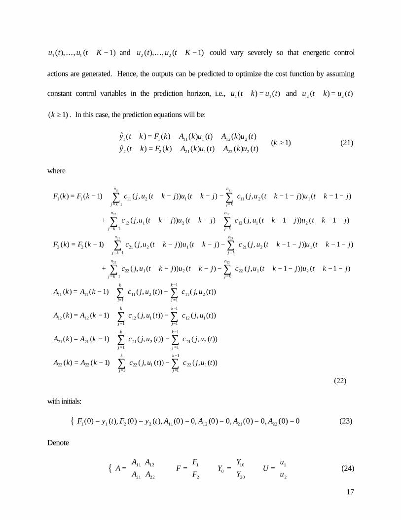
17

u t u t K1 1 1( ), ..., ( )+ − and u t u t K2 2 1( ),..., ( )+ − could vary severely so that energetic control

actions are generated. Hence, the outputs can be predicted to optimize the cost function by assuming

constant control variables in the prediction horizon, i.e., u t k u t1 1( ) ( )+ = and u t k u t2 2( ) ( )+ =

( )k ≥ 1 . In this case, the prediction equations will be:

$ ( ) ( ) ( ) ( ) ( ) ( )

$ ( ) ( ) ( ) ( ) ( ) ( )( )

y t k F k A k u t A k u t

y t k F k A k u t A k u tk1 1 11 1 12 2

2 2 21 1 22 2

1+ = + ++ = + +

≥ (21)

where

F k F k c j u t k j u t k j c j u t k j u t k j

c j u t k j u t k j c j u t k j u t k j

F k F k c j u

j k

n

j k

n

j k

n

j k

n

j k

n

1 11

11 2 1 11 2 1

112 1 2 12 1 2

2 21

21 2

1 1 1

1 1

1

11 11

12 12

21

( ) ( ) ( , ( )) ( ) ( , ( )) ( )

( , ( )) ( ) ( , ( )) ( )

( ) ( ) ( , (

= − + + − + − − + − − + − −

+ − + − − + − − + − −

= − +

= + =

= + =

= +

∑ ∑

∑ ∑

∑

+

t k j u t k j c j u t k j u t k j

c j u t k j u t k j c j u t k j u t k j

A k A k c j u t c j u t

A k A k

j k

n

j k

n

j k

n

j

k

j

k

+ − + − − + − − + − −

+ − + − − + − − + − −

= − + −

= −

=

= + =

= =

−

∑

∑ ∑

∑ ∑

)) ( ) ( , ( )) ( )

( , ( )) ( ) ( , ( )) ( )

( ) ( ) ( , ( )) ( , ( ))

( ) ( )

1 21 2 1

122 1 2 22 1 2

11 111

11 21

1

11 2

12 12

21

22 22

1 1

1 1

1

1

+

+ −

= − + −

= − + −

= =

−

= =

−

= =

−

∑ ∑

∑ ∑

∑ ∑

j

k

j

k

j

k

j

k

j

k

j

k

c j u t c j u t

A k A k c j u t c j u t

A k A k c j u t c j u t

112 1

1

1

12 1

21 211

21 21

1

21 2

22 221

22 11

1

22 1

1

1

( , ( )) ( , ( ))

( ) ( ) ( , ( )) ( , ( ))

( ) ( ) ( , ( )) ( , ( ))

(22)

with initials:

{ F y t F y t A A A A1 1 2 2 11 12 21 220 0 0 0 0 0 0 0 0 0( ) ( ), ( ) ( ), ( ) , ( ) , ( ) , ( )= = = = = = (23)

Denote

{ AA A

A A=

11 12

21 22

F

F

F=

1

2

YY

Y010

20

=

U

u

u=

1

2

(24)

18

Then the cost function (20) can be written as:

G F K Y A K U t F K Y A K U tT= − − − −( ( ) ( ) ( )) ( ( ) ( ) ( ))0 0 (20' )

It can be seen from (22) that A K( ) depends on U t( ) being determined. Hence, minimization of G

with respect to U t( ) is a non-linear optimization problem.

In order to obtain an exact numerical solution of a non-linear optimization, an iterative calculation is

needed. For a real-time control, an on-line iterative calculation is not preferred. Hence, the necessity of

implementing an on-line iterative calculation for achieving an exact numerical solution should be argued.

It is known that the neurofuzzy model identified is a nominal model of the welding process. The

unavoidable variations in the welding conditions such as the heat transfer condition cause the actual

dynamics to differ from the nominal model. In this case, an exact numerical solution of the non-linear

optimization based on the nominal model may not exactly optimize the actual cost function. The error

increases as the uncertainty of the process increases. For the welding process, the uncertainty which

makes the closed-loop control necessary is substantial [8, 31]. Also, since there is no constraint on the

change of the control action U t( ) -U t( )− 1 , U t( ) determined based on the non-linear optimization of

(20) or (20’) could significantly differ from U t( )− 1 . As a result, the control actions could be very

energetic so that the resultant weld appearance is not smooth. Also, the large changes of the control

actions and the significant difference between the actual dynamics and the nominal model could cause

severe errors between the predicted and actual outputs. The closed-loop system could be unstable.

Hence, the following modified cost function is used:

J F K Y A K U t F K Y A K U t U t U t U t U tT T= − − − − + − − − −( ( ) ( ) ( )) ( ( ) ( ) ( )) ( ( ) ( )) ( ( ) ( ))0 0 1 1Λ (25)

where Λ = diag( , )λ λ1 2 ( , )λ λ1 20 0≥ ≥ are the weights.

19

When the amplitudes of U t( ) -U t( )− 1 are not large, c j u t s11 2( , ( ))' ... can be approximated by

c j u t s11 2 1( , ( ))'− .... so that A K( ) can be calculated before the optimization. (The resultant accuracy

in calculating A K( ) depends on the actual amplitudes of U t( ) -U t( )− 1 .) Hence, the optimization

becomes linear. The analytic solution is:

U t A K A K A K F K A K Y U tT T T( ) ( ( ) ( ) ) ( ( ) ( ) ( ) ( ))= + − + −−Λ Λ10 1 (26)

The values of the weights λ1 and λ2 can be determined based on their physical meaning in correlating

the preferred changes of the control actions to the errors between the desired and measured outputs. In

the developed system, λ1 =102 ( / )mm A100 2 is selected. This implies that an error of 1 mm in the

predicted and desired top-side or back-side bead width has the same contribution to the cost function

as u t u t1 1 1 0 1( ) ( ) .− − = , i.e., 10 A because the unit of u1 in our control system is 100 A, does.

Similarly, λ2 =10 2 ( )mm 2 2 is selected.

7. CLOSED-LOOP CONTROL EXPERIMENTATION

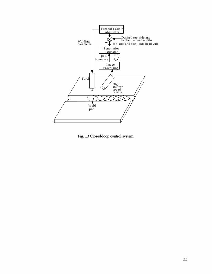
The developed closed-loop control system can be illustrated using the diagram in Fig. 13. In order

to examine the robustness of the developed control system, uncertainties are emulated using a number of

artificial disturbances in the closed-loop control experiments.

7.1 Experiment 1: Step Change of Rate of the Shielding Gas

In arc welding, the weld pool and electrode are prevented from being contaminated by the

atmosphere by applying the shielding gas. In terms of circuit, the arc column can be regarded as a

resistor in which the welding current flows and its resistance depends on both the arc length and

shielding gas. The shielding gas, either the type or rate of the flow, has an influence on the welding arc,

and therefore influences the weld pool.

20

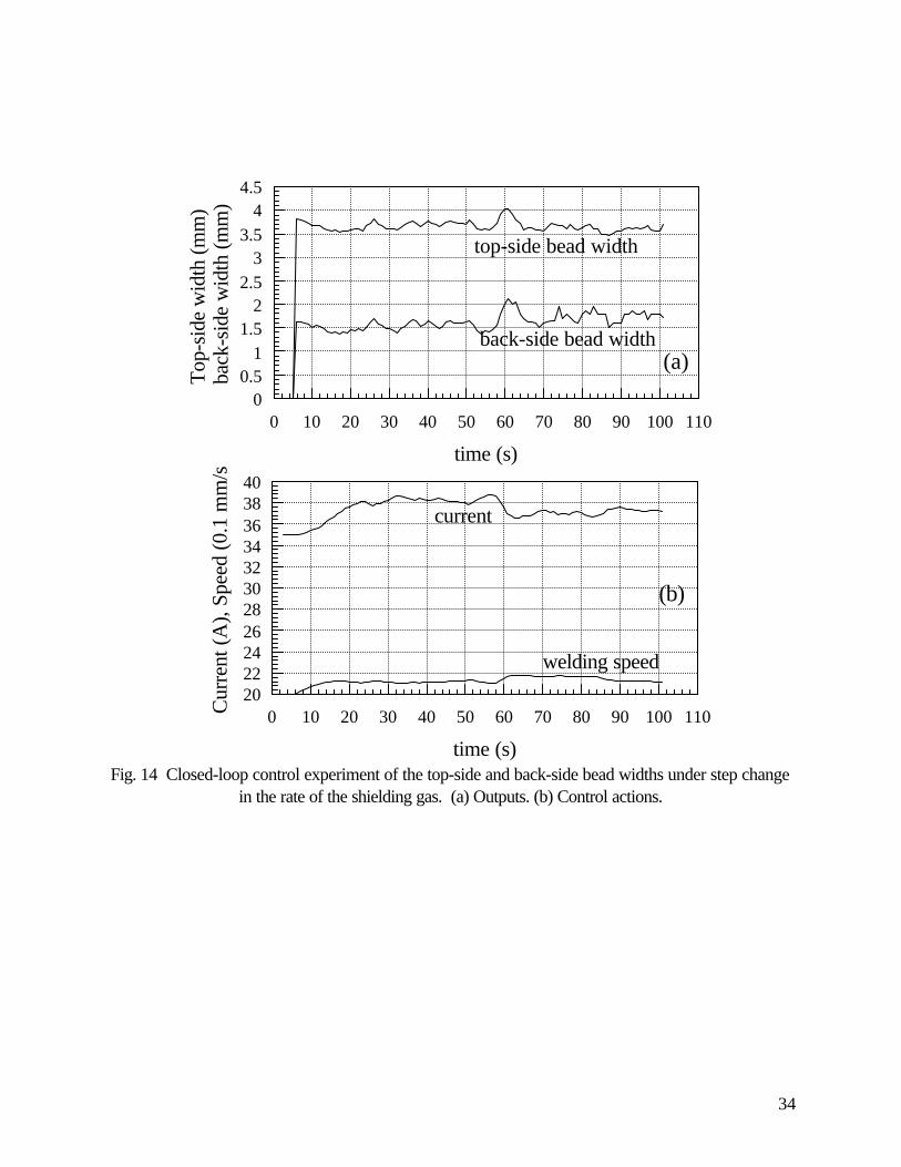
In this experiment, the initial rate of the argon flow was 27 l/min. At t s= 55 , the rate changes to 10

l/min (Fig. 14). As a result, both the top-side and back-side bead widths increase. As it can be

observed in Fig. 14, by decreasing the welding current and increasing the welding speed, the closed-

loop control system successfully eliminates the influence of the decrease in the rate of the argon flow.

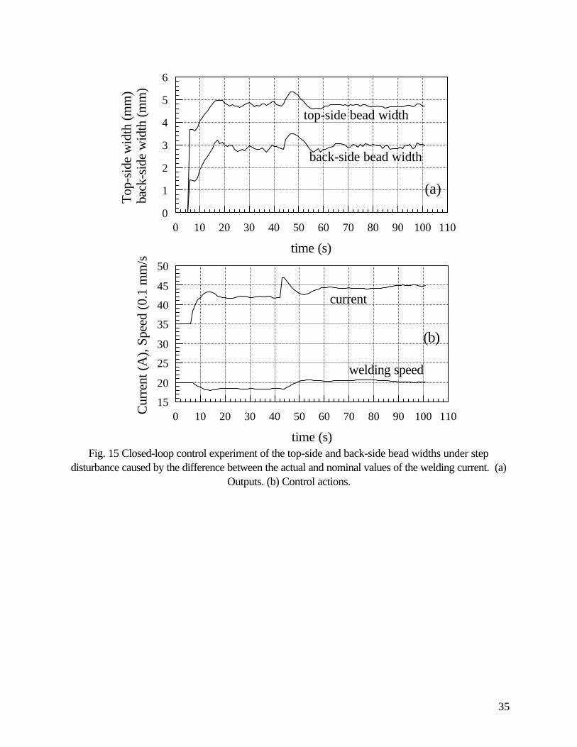
7.2 Experiment 2: Current Disturbance

In this experiment, an artificial error between the actual and nominal values of the welding current is

applied. During the first 42 seconds, no error exists between the actual and nominal values. From

t s= 42 , the actual current is 5 A larger than the nominal value. Hence, both the top-side and back-

side bead widths increases. As it can be seen in Fig. 15, the welding current and speed immediately

decreases and increases, respectively, so that the outputs can be maintained at the desired levels again.

We notice that for advanced welding systems, such an error between the actual and nominal values

of the welding current may not be frequently encountered. However, this artificial disturbance can

change the dynamic model which correlates the outputs to the nominal values of the welding parameters.

Hence, a model perturbation is emulated.

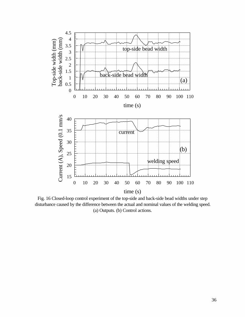
7.3 Experiment 3: Speed Disturbance

In this experiment, an artificial error between the actual and nominal values of the welding speed is

applied. During the first 52s seconds, no error exists between the actual and nominal values. However,

after t s= 52 , the actual welding speed is 0.5 mm/s smaller than the nominal value. At t s= 52 , the

welding current and speed are about 38 A and 2.2 mm/s, respectively. If no closed-loop correction is

applied, 38 A welding current and 1.7 mm/s welding speed will increase the top-side and back-side

bead widths by about 2 mm. Fig. 16 shows that this disturbance has been overcome by the closed-

loop control system by simultaneously changing the welding current and welding speed.

21

Unlike the error between the actual and nominal values of the welding current, the error between the

actual and nominal values of the welding speed can often be met in many applications. Hence, in

addition to the emulation of the model perturbation, this experiment also shows that the developed

closed-loop control system is robust with respect to the possible variation in the welding speed.

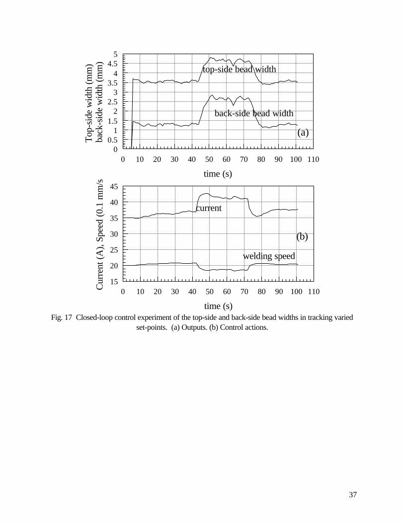
7.4 Experiment 4: Tracking Varying Set-Points

Fig. 17 shows a closed-loop control experiment in tracking varied set-points. In general, the

dynamic properties of the non-linear process vary with the operating points. In order to track the varied

set-points, the operating points have to change. If a linear controller is used, the performance of the

closed-loop control will in general not be guaranteed for different operating points. The welding

experiment in Fig. 17 shows that the varied set-points are well tracked. The similar results have also

been observed in other experiments that tracked other varied set-points.

8. CONCLUSIONS

The non-linearity of the controlled process which has the welding current and speeds as the inputs

and back-side and top-side bead widths as the outputs is fundamental. The neurofuzzy model can

describe the dynamic non-linear process being controlled with sufficient accuracy. A neurofuzzy model

based predictive algorithm has been developed to control the non-linear welding process. The control

experiments showed that the desired fusion state can be achieved by using the developed control system

despite severe disturbances.

The developed system provides a solution to precise control of welding process. It is currently being

used to weld aerospace materials. In applications where the requirement on the accuracy is relatively

low and where the variations in the welding conditions are insignificant, other simpler control algorithms

may also be used to ease the system design.

22

ACKNOWLEDGEMENT

The authors would like to thank Mr. Lin Li at the Center for Robotics and Manufacturing Systems

Welding Research and Development Laboratory for his significant contributions in programming, data

processing, and experimenting.

REFERENCES

1. Vorman, A. R., and Brandt, H., 1976. Feedback control of GTA welding using puddle widthmeasurement, Welding Journal, 55(9): 742-749.

2. Chen, W., and Chin, B. A., 1990. Monitoring joint penetration using infrared sensing techniques.Welding Journal, 69(4): 181s-185s.

3. Banerjee, P., et al., 1995. Infrared sensing for on-line weld geometry monitoring and control.ASME Journal of Engineering for Industry, 117(3): 323-330.

4. Richardson, R. W. et al., 1984. Coaxial arc weld pool viewing for process monitoring and control.Welding Journal, 63(3): 43-50.

5. Pietrzak, K. A. and Packer, S. M., 1994. Vision-based weld pool width control. ASME Journalof Engineering for Industry, 116(1): 86-92.

6. Song, J.-B., and Hardt, D. E., 1994. Dynamic modeling and adaptive control of the gas metal arcwelding process. ASME Journal of Dynamic Systems, Measurement, and Control, 116(3):405-413.

7. Zhang, Y. M., et al., 1993. Determining joint penetration in GTAW with vision sensing of weld-face geometry. Welding Journal, 72(1): 463s-469s.

8. Zhang, Y. M., Kovacevic, R. and Wu, L., 1996. Dynamic analysis and identification of gastungsten arc welding process for full penetration control. ASME Journal of Engineering forIndustry, 118(1): 123-136.

9. Zhang, Y. M., Kovacevic, R., and Li, L., 1996. Robust adaptive control of full penetration GTAwelding. IEEE Transactions on Control Systems Technology, 4(4): 394-403.

10. Kovacevic, R., Zhang, Y. M. and Ruan, R., 1995. Sensing and control of weld pool geometry forautomated GTA welding. ASME Journal of Engineering for Industry, 117(2): 210-222.

11. Hoffman, T., 1991. Real-time imaging for process control. Advanced Material & Processes,140(3): 37-43.

12. Kovacevic, R. and Zhang, Y. M., 1997. Neurofuzzy model-based weld fusion state estimation.IEEE Control Systems Magazine, 17(2): 30-42.

13. ASM Handbook, Vol. 6, Welding, Brazing, and Soldering, 1993, pp. 30-35.14. Jang, J. S. R. and Sun, C. T., 1995. Neuro-fuzzy logic modeling and control. Proceedings of the

IEEE, 83(3): 378-406.15. Mamdani, E. H., and Assilian, S., 1975. An experiment in linguistic synthesis with a fuzzy logic

controller. International Journal of Machine Studies, 7(1): 1-13.16. Du, R., Elbestawi, M. A., and Wu, S. M., 1995. Automated monitoring of manufacturing

processes, part 1: monitoring methods. ASME Journal of Engineering for Industry, 117(2):121-132.

23

17. Ko, T. J. and Cho, D. W., 1994. Tool wear monitoring in diamond turning by fuzzy patternrecognition. ASME Journal of Engineering for Industry, 116(2): 225-232.

18. Billatos, S. B. and Webster, J. A., 1993. Knowledge-based expert system for ballscrew grinding.ASME Journal of Engineering for Industry, 115(2): 239-235.

19. Fang, X. D., 1995. Expert system-supported fuzzy diagnosis finish-turning process states.International Journal of Machine Tools and Manufacture, 35(6): 913-924.

20. Brown, M. and Harris, C., 1994. Neurofuzzy adaptive modeling and control. Prentice Hall,New York.

21. Tanaka, K, Sano, M., and Watanabe, H., 1995. Modeling and control of carbon monoxideconcentration using a neuro-fuzzy technique. IEEE Transactions on Fuzzy Systems, 3(3): 271-279.

22. Hayashi, K., et al., 1995. Neuro fuzzy transmission control for automobile with variable loads.IEEE Transactions on Control Systems Technology. 3(1): 49-53.

23. Sharaf, A. M. and Lie, T. T., 1994. Neuro-fuzzy hybrid power system stabilizer. Electric PowerSystems Research, 30(1): 17-23.

24. Mesina, O. S. and Langari, R., 1994. Neuro-fuzzy system for tool condition monitoring in metalcutting. in Dynamic Systems and Control, Vol. 2, pp. 931-938, 1994 ASME InternationalMechanical Engineering Congress, ASME.

25. Takagi, T., and Sugeno, M., 1985. Fuzzy identification of systems and its applications to modelingand control. IEEE Transactions on Systems, Man, and Cybernetics, 15(1): 116-132.

26. Parker, D. B., 1987. Optimal algorithms for adaptive networks: second order back propagation,second order direct propagation, and second order {H}ebbian learning. Proceedings of IEEEInternational Conference on Neural Networks, pp. 593-600.

27. Using NeuralWorks. NeuralWare, Inc., Pittsburgh, PA, 1993.28. Haykin, S., 1994. Neural networks: a comprehensive foundation. Macmillan College

Publishing Company, New York.29. Clarke, D. W., Mohtadi, C., and Tuffs, P. S., 1987. Generalized predictive control-part 1: the

basic algorithm. Automatica, Vol. 23, pp. 137-148.30. de Oliveira, J. V. and Lemos, J. M., 1995. Long-range predictive adaptive fuzzy relational control.

Fuzzy Sets and Systems, 70(2-3): 337-357.31. Mills, K. C. and Keene, B. J., 1990. Factors affecting variable weld penetration. International

Materials Reviews, 35(4): 185-216.

24

CAPTIONS OF FIGURES AND TABLES

Fig. 1 Fusion parameters of fully penetrated weld pool.

Fig. 2 Gas tungsten arc welding.

Fig. 3 Weld pools made using different welding speeds. Current: 100 A, arc length: 3mm, 3mm 304stainless steel. (a). 2.92mm/s, (b) 2.42mm/s, (c) 1.95 mm/s, (d) 1.43mm/s.

Fig. 4 Weld pools made using different currents. Arc length: 3mm, speed: 1.9 mm/s, 3mm 304stainless steel. (a). 95 A, (b) 105 A, (c) 110 A, (d) 115 A.

Fig. 5 1 1/ ~ /v v .

Fig. 6 Empirical static correlations between the welding current and weld pool parameters.(a). L i~ . (b). w i~ . The experimental data in Fig. 4 are used.

Fig. 7 Experimental set-up.

Fig. 8 Inputted welding parameters for the five dynamic experiments.

Fig. 9 Measured pool parameters from the five dynamic experiments.

Fig. 10 Distribution of inputs in the dynamic experiments.

Fig. 11 Neurofuzzy modeling results. (a) Back-side bead width y1 (b) Top-side bead width y2 .

Fig. 12 Linear modeling (without variable partition). (a) Back-side bead width y1 (b) Top-side beadwidth y2 .

Fig. 13 Closed-loop control system.

Fig. 14 Closed-loop control experiment of the top-side and back-side bead widths under step changein the rate of the shielding gas. (a) Outputs. (b) Control actions.

Fig. 15 Closed-loop control experiment of the top-side and back-side bead widths under stepdisturbance caused by the difference between the actual and nominal values of the welding current. (a)Outputs. (b) Control actions.

Fig. 16 Closed-loop control experiment of the top-side and back-side bead widths under stepdisturbance caused by the difference between the actual and nominal values of the welding speed.(a) Outputs. (b) Control actions.

25

Fig. 17 Closed-loop control experiment of the top-side and back-side bead widths in tracking variedset-points. (a) Outputs. (b) Control actions.

Table 1 Fuzzy partition of control variables

Table 2 Identified fuzzy partition parameters

Table 3 Identified c j i11 2( / ) ’s

Table 4 Identified c j i12 1( / ) ’s

Table 5 Identified c j i21 2( / ) ’s

Table 6 Identified c j i22 1( / ) ’s

Back-side bead width

Molten pool

Unmolten or solidified material

Top-side pool width

Outline of fusion zone

Fig. 1 Fusion parameters of fully penetrated weld pool.

Direction ofwelding

Currentconductor

Shieldinggas in

Nonconsumabletungsten electrode

Gas shield

Arc

Solidifiedweld metal

Gasnozzle

Powersource

Weld poolBase metal

TORCH

Fig. 2 Gas tungsten arc welding.

26

(a) (b) (c) (d)

Fig. 3 Weld pools made using different welding speeds. Current: 100 A, arc length: 3mm, 3mm 304 stainless steel. (a). 2.92mm/s, (b) 2.42mm/s, (c) 1.95 mm/s, (d) 1.43mm/s.

(a) (b) (c) (d)

Fig. 4 Weld pools made using different currents. Arc length: 3mm, speed: 1.9 mm/s, 3mm 304 stainless steel. (a). 95 A, (b) 105 A, (c) 110 A, (d) 115 A.

0.5 0.6 0.7 0.8 0.9 1 1.1 1.2 1.3 1.4 1.5

1/v1/2 (1/mm1/2)

0.20.40.60.8

11.21.41.61.8

2

1/v

(1/m

m)

v: [0.5 mm, 4 mm]

Fig. 5 1 1/ ~ /v v .

95 100 105 110 115i (A)

5.25.45.65.8

66.26.4

w (m

m)

(a)

95 100 105 110 115

i (A)

6.57

7.58

8.59

9.510

10.5

L (m

m)

(b)

Fig. 6 Empirical static correlations between the welding current and weld pool parameters.(a). L i~ . (b). w i~ . The experimental data in Fig. 4 are used.

27

Power Supply

Interface

3-axis motion control board

3-axial Manipulator

Computer

Frame Grabber

MonitorCurrent

VideoSignal

Camera

Torch

Speed

LaserOptical Fiber

Weld Pool

Travel Direction

yi

x

z

y

xi

Fig. 7 Experimental set-up.

20 25 30 35 40 45 50 55 60 65 70

Time (s)

10

20

30

40

50

60

70

v(0.

1mm

/s),

i(A

)

(a)

i

v

20 30 40 50 60 70 80 90 100

Time (s)

10

20

30

40

50

60

70

80

v(0.

1mm

/s),

i(A

)

(b)

i

v

60 65 70 75 80 85 90 95 100

Time (s)

20

25

30

35

40

45

50

55

v(0.

1mm

/s),

i(A

)

(c)

i

v

60 65 70 75 80 85 90 95 100

Time (s)

510152025303540455055

v(0.

1mm

/s),

i(A

)

(d)

v

i

28

0 10 20 30 40 50 60 70 80 90 100

Time (s)

10

20

30

40

50

60

70

v(0.

1mm

/s),

i(A

)

(e)

v

i

Fig. 8 Inputted welding parameters for the five dynamic experiments.

29

20 25 30 35 40 45 50 55 60 65 70

Time (s)

123456789

101112

L(m

m),

w(m

m),

wb(m

m)

(a)

L

w

wb

20 30 40 50 60 70 80 90 100

Time (s)

2

4

6

8

10

12

14

L(m

m),

w(m

m),

wb(m

m)

(b)

L

w

wb

60 65 70 75 80 85 90 95 100

Time (s)

11.5

22.5

33.5

44.5

55.5

6

L(m

m),

w(m

m),

wb(m

m)

(c)

L

w

wb

60 65 70 75 80 85 90 95 100

Time (s)

23456789

101112

L(m

m),

w(m

m),

wb(m

m)

(d)

L

w

wb

30

0 10 20 30 40 50 60 70 80 90 100

Time (s)

2

4

6

8

10

12

14

L(m

m),

w(m

m),

wb(m

m) (e)

L

w

wb

Fig. 9 Measured pool parameters from the five dynamic experiments.

35 40 45 50 55 60 65 70 75

Current (A)

0.5

1

1.5

2

2.5

3

3.5

Wel

ding

Spe

ed (

mm

/s)

Projected Range ofControlVariables

Fig. 10 Distribution of inputs in the dynamic experiments.

31

0 500 1,000 1,500 2,000 2,500

Discrete instant

1

2

3

4

5

6

7

wb

(mm

)

Measured Model Predicted

(a)

0 500 1,000 1,500 2,000 2,500

Discrete instant

2.53

3.54

4.55

5.56

6.57

7.5

w (m

m)

Measured Model Predicted

(b)

Fig. 11 Neurofuzzy modeling results. (a) Back-side bead width y1 (b) Top-side bead width y2 .

0 500 1,000 1,500 2,000 2,500

Discrete instant

11.5

22.5

33.5

44.5

55.5

6

wb

(mm

)

Measured Model Predicted

(a)

32

0 500 1,000 1,500 2,000 2,500

Discrete instant

2.53

3.54

4.55

5.56

6.57

7.5

w (m

m)

Measured Model Predicted

(b)

Fig. 12 Linear modeling (without variable partition). (a) Back-side bead width y1 (b) Top-side beadwidth y2 .

33

Torch

Highshutterspeed camera

ImageProcessing

Penetration Estimator

Feedback Control Algorithm

pool boundary

top-side and back-side bead widths

Desired top-side and back-side bead widthsWelding

parameters

Weld pool

Fig. 13 Closed-loop control system.

34

0 10 20 30 40 50 60 70 80 90 100 110

time (s)

00.5

11.5

22.5

33.5

44.5

Top

-sid

e w

idth

(mm

) ba

ck-s

ide

wid

th (m

m)

top-side bead width

back-side bead width(a)

0 10 20 30 40 50 60 70 80 90 100 110

time (s)

2022242628303234363840

Cur

rent

(A),

Spee

d (0

.1 m

m/s

)

current

welding speed

(b)

Fig. 14 Closed-loop control experiment of the top-side and back-side bead widths under step changein the rate of the shielding gas. (a) Outputs. (b) Control actions.

35

0 10 20 30 40 50 60 70 80 90 100 110

time (s)

0

1

2

3

4

5

6

Top

-sid

e w

idth

(mm

) ba

ck-s

ide

wid

th (m

m)

top-side bead width

back-side bead width

(a)

0 10 20 30 40 50 60 70 80 90 100 110

time (s)

15

20

25

30

35

40

45

50

Cur

rent

(A),

Spee

d (0

.1 m

m/s

)

current

welding speed

(b)

Fig. 15 Closed-loop control experiment of the top-side and back-side bead widths under stepdisturbance caused by the difference between the actual and nominal values of the welding current. (a)

Outputs. (b) Control actions.

36

0 10 20 30 40 50 60 70 80 90 100 110

time (s)

00.5

11.5

22.5

33.5

44.5

Top

-sid

e w

idth

(mm

) ba

ck-s

ide

wid

th (m

m)

top-side bead width

back-side bead width(a)

0 10 20 30 40 50 60 70 80 90 100 110

time (s)

15

20

25

30

35

40

Cur

rent

(A),

Spee

d (0

.1 m

m/s

)

current

welding speed

(b)

Fig. 16 Closed-loop control experiment of the top-side and back-side bead widths under stepdisturbance caused by the difference between the actual and nominal values of the welding speed.

(a) Outputs. (b) Control actions.

37

0 10 20 30 40 50 60 70 80 90 100 110

time (s)

00.5

11.5

22.5

33.5

44.5

5

Top

-sid

e w

idth

(mm

) ba

ck-s

ide

wid

th (m

m)

top-side bead width

back-side bead width

(a)

0 10 20 30 40 50 60 70 80 90 100 110

time (s)

15

20

25

30

35

40

45

Cur

rent

(A),

Spee

d (0

.1 m

m/s

)

current

welding speed

(b)

Fig. 17 Closed-loop control experiment of the top-side and back-side bead widths in tracking variedset-points. (a) Outputs. (b) Control actions.

38

Table 1 Fuzzy partition of control variablesFuzzy variables Number of fuzzy sets Partition u1 I1 4= low ( A11 ) , middle ( A12 ) ,

high ( A13 ) , very high( A14 ) u2 I2 4= small( A21) ,moderate ( A22 ) ,

large ( A23 ) , very large ( A24 )

Table 2 Identified fuzzy partition parametersk = 1 k = 2 k = 3 k = 4

a k1 0.30 0.43 0.56 0.7a k2 0.30 0.53 0.76 1.0b k1 ( . )×0 001 8.45 8.45 8.45 8.45b k2 ( . )×0 01 2.64 2.64 2.64 2.64

Table 3 Identified c j i11 2( / ) ’si2 1= i2 2= i2 3= i2 4=

j = 1 2.54 1.50 1.42 .85j = 2 .096 .36 .46 .37j = 3 1.96 1.64 1.27 0.54j = 4 -3.04 -1.68 -0.12 -0.40

Table 4 Identified c j i12 1( / ) ’si1 1= i1 2= i1 3= i1 4=

j = 1 -0.10 1.42 1.95 1.66j = 2 -1.01 .723 .850 2.29j = 3 .078 1.38 1.43 0.92j = 4 -2.08 -0.47 -0.11 3.9

Table 5 Identified c j i21 2( / ) ’si2 1= i2 2= i2 3= i2 4=

j = 1 3.45 2.75 2.16 .711j = 2 .703 .875 .614 -0.03j = 3 .712 .444 .382 -0.22j = 4 -1.90 -1.54 -0.41 -0.56

Table 6 Identified c j i22 1( / ) ’si1 1= i1 2= i1 3= i1 4=

j = 1 1.48 2.06 2.49 2.28j = 2 .703 1.21 1.54 2.73

39

j = 3 .207 .933 1.35 .950j = 4 -1.48 -0.04 .373 1.96