Embed Size (px)
Citation preview
5 Intelligent Neurofuzzy Control of a Robotic Gripper
J. A. Domínguez-López, R.I. Damper, R.M. Crowder and C.J. Harris
Department of Electronics and Computer Science, University of South-ampton, Southampton, UK. email: {jadl00r|rid|rmc|cjh}@ecs.soton.ac.uk.
5.1 Introduction
One of the major challenges of robotics is the grasping and manipulating of objects in an unstructured environment, in particular where the physical properties of the object are not known a priori. The resultant uncertainty makes it difficult to control contact forces, and the relative position be-tween the object and the gripper’s point of contact. As part of the grasping process, force control is required. This will avoid the risk of the object slipping out of the end effector as well as any possible damage to the ob-ject. The means of defining the required grasp force is crucial and can be posed as an optimisation problem, [1].
Various techniques have been applied to solve this problem [2-4] Some approaches are analytic and cannot be easily implemented in real-time ap-plications, when dynamic adaptation to external disturbances is an impor-tant requirement. Also, the analytic approach cannot be used if variables such as the object’s weight and end effector acceleration are unknown. To overcome this situation, other approaches using fuzzy controllers have been developed using a number of different sensors to measure the physi-cal variables which provide feedback to the system. Fuzzy systems have a number of advantages over traditional techniques that make them an attractive approach to solve this type of problem. Some of these general advantages are their ability to model complex and/or non-linear problems, to mimic human decisions handling vague concepts, rapid computation due to intrinsic parallel processing, capacity to deal with imprecise information, improved knowledge representation and better uncertain reasoning than traditional techniques. However, fuzzy systems have also several disadvantages including mathematical opaqueness, they are highly abstract and heuristic, and they need an expert (or operator) for rule
156 J. A. Domínguez-López, R.I. Damper, R.M. Crowder and C.J. Harris
and heuristic, and they need an expert (or operator) for rule discovery. They are unable to adapt by themselves in response to changes in process parameters because in a purely fuzzy system the parameters do not appear in an analytical form so they cannot be easily modified for learning and tuning the fuzzy rules, [5]. Nevertheless, fuzzy control can be used in con-junction with powerful automatic learning methods (i.e., neural networks) as a neurofuzzy system [6-8].
In this chapter, we explore these issues using a very simple two-fingered gripper as an experimental system. Work is conducted both using a real gripper and, because of the high degree of flexibility it affords, in software simulation. The structure of the chapter is as follows. In Section 5.2, we describe these two experimental systems. Section 5.3 then outlines aspects of neurofuzzy systems as they impact on this study. Since machine learn-ing methods to allow such systems to adapt to their environment are a ma-jor concern, these are discussed in some detail in Section 5.4. Results of applying our methods to the design of an adaptive neurofuzzy controller for the real gripper are described in Section 5.5. We then turn to the simu-lation of the gripper mounted on a six degree of freedom robot in Section 5.6, before concluding in Section 5.7.
5.2 Experimental Systems
The work reported in this chapter has used two different experimental sys-tems: a simple, low-cost two-fingered gripper and a simulation system written by the first author. Ideally, we would have liked to do all our work with real robotic systems but this is inflexible and expensive in terms of hardware. Hence, the simple system was used to prove our ideas which were then further explored in simulation.
5.2.1 Two fingered gripper
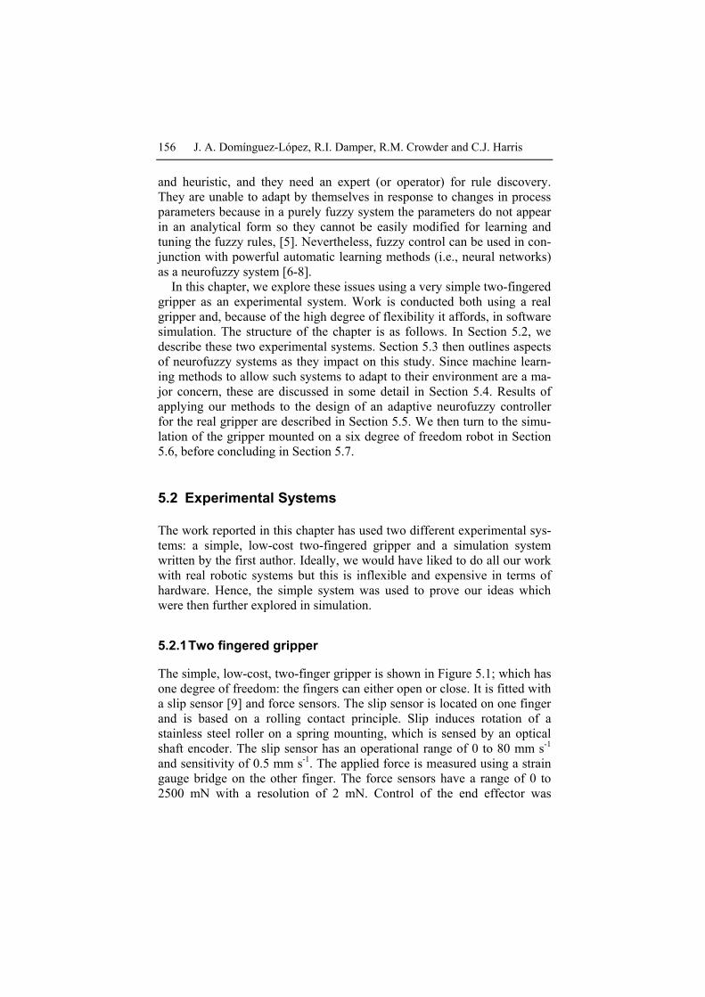
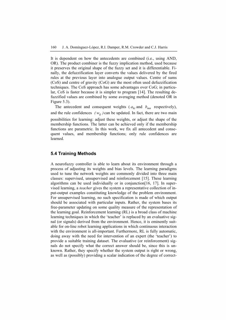
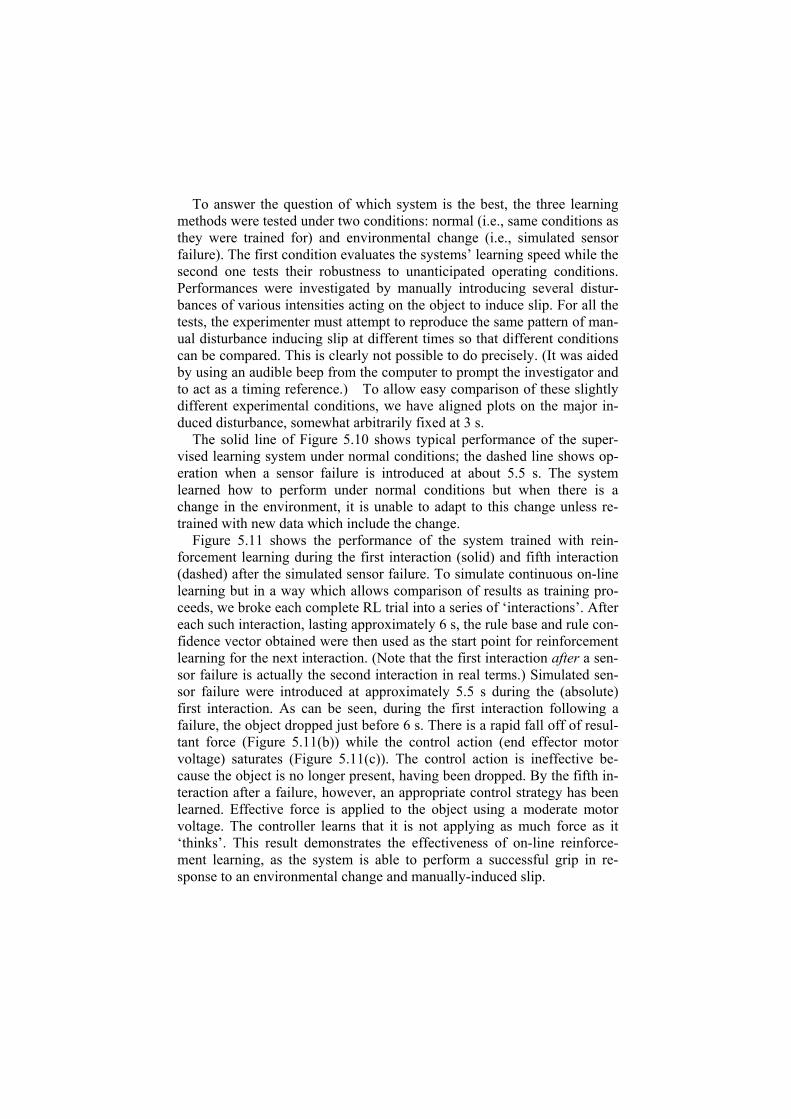
The simple, low-cost, two-finger gripper is shown in Figure 5.1; which has one degree of freedom: the fingers can either open or close. It is fitted with a slip sensor [9] and force sensors. The slip sensor is located on one finger and is based on a rolling contact principle. Slip induces rotation of a stainless steel roller on a spring mounting, which is sensed by an optical shaft encoder. The slip sensor has an operational range of 0 to 80 mm s-1 and sensitivity of 0.5 mm s-1. The applied force is measured using a strain gauge bridge on the other finger. The force sensors have a range of 0 to 2500 mN with a resolution of 2 mN. Control of the end effector was
5 Intelligent Neurofuzzy Control of a Robotic Gripper 157
achieved using a personal computer (Pentium 75 MHz, 64 MB RAM) fit-ted with a high-speed analogue input/output card (Eagle Technologies PC30GAS4). Control software ran under the MS-DOS operating system,. The sampling period for the system was set conservatively to 17 ms to al-low adequate time for all processing to be complete between consecutive samples.
Figure 5.1 The experimental, two-fingered gripper. The slip sensor appears on the left of the picture, attached to one of the fingers. The force sensors (strain gauges) are attached approximately midway along the finger shown on the right of the pic-ture.
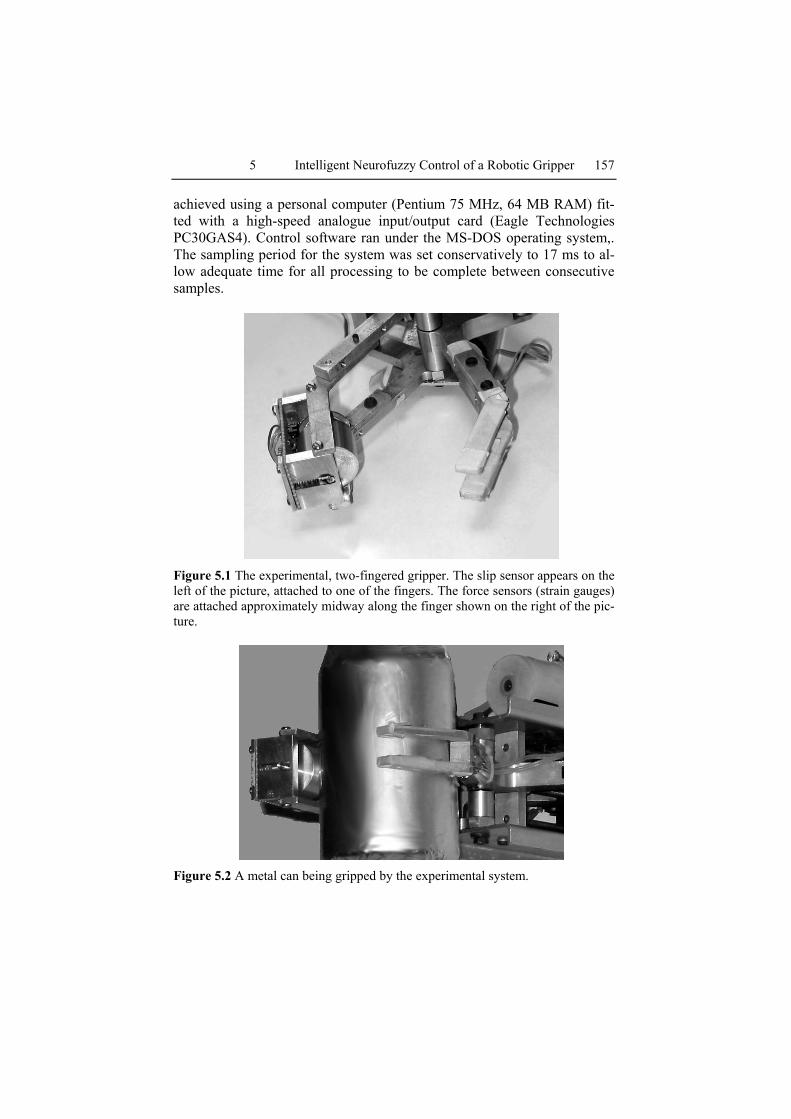
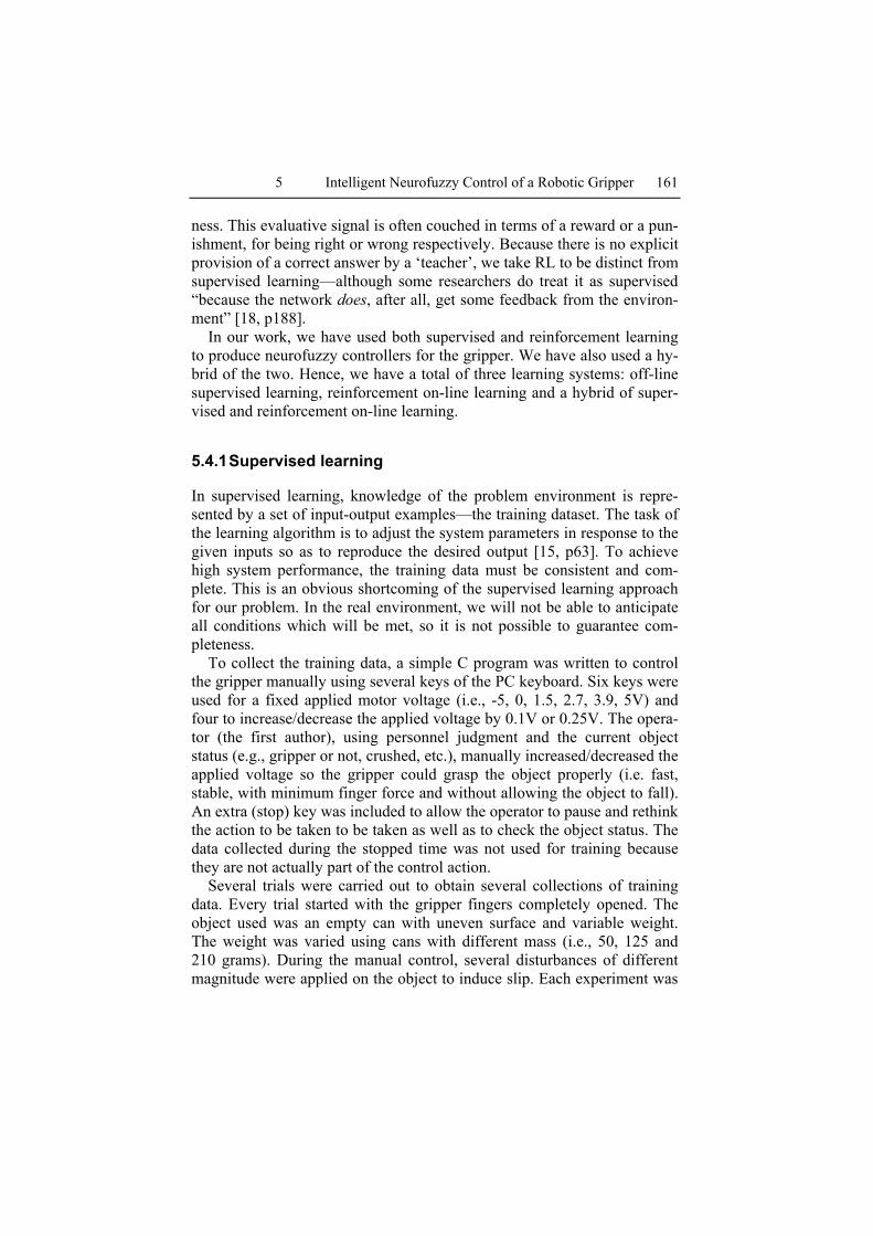
Figure 5.2 A metal can being gripped by the experimental system.
158 J. A. Domínguez-López, R.I. Damper, R.M. Crowder and C.J. Harris
Figure 5.2 shows metal can being gripped by the experimental system. The roller of the slip sensor is clearly visible, together with its spring mounting which prevents the sensor from seizing during gripping. This metal can was found to be an effective vehicle for our experiments, as the total weight of the gripped object could be conveniently manipulated by placing various weights in it (see Section 5.5).
5.2.2 Simulation
In this part of the work, a simulated gripper was subjected to a range of identical load disturbances. The gripper was the simple two-fingered, sin-gle degree of freedom system with slip and force sensors, as described above. Full details of the simulation’s kinematics equations can be found in Appendix A of [10]. The simulation was validated against results of the real gripper handling a range of weights.
The gripper was simulated holding a 0.1kg object. An external transient force of 10 N was applied to the load 3 seconds into the simulation, and a second force of -10 N was applied at 5 seconds. Between 6 and 10 sec-onds, the gripper was moved, thereby applying acceleration forces along its z-axis.
5.3 Neurofuzzy Systems
Neurofuzzy systems combine the advantages of fuzzy systems, such as transparent representation of knowledge, and those of neural networks, which deal with implicit knowledge that can be acquired by means of learning [8, 11, 12]. They mimic human decision processes, in that they manage imprecise, partial, vague or imperfect information. Also, they are able to resolve conflicts by collaboration and aggregation. Moreover, they have self-learning, self-organising and self-tuning capabilities, with no re-quirement for prior knowledge of relationships of data although they can use this if it is available. They have fast computation using fuzzy number operations. As do fuzzy systems, neurofuzzy systems embody rules (de-fined in a linguistic way) so that system operation can be interpreted in a transparent fashion.
5 Intelligent Neurofuzzy Control of a Robotic Gripper 159
.
.
.
.
.
.
Inputs
Fuzzification
layerFuzzy rule
layer
Weightof rules
Defuzzification layer
OutputRulesAntecedent(IF is )x A
.
.
.
.
.
.
.
Consequent(THEN y is B)
Antecedentweight
ConsequentweightGrade
11
12
1N1
iNi
i2
i1
� (x )A111
1
11
12
1M
w
w
w
11
22
MP
a11
a22
a1R+1
a2R+2
aP2
aPQ
b11
b12
b1M
B
B
B� (x )A12
1
� (x )A1N1A
OR
Rule P
Rule 2
Rule 1
� (x )Ai1i
� (x )Ai2i
i
� (x )AiN i
A
A
A
A
A
Y(t)
x (t)
x (t)
1
i
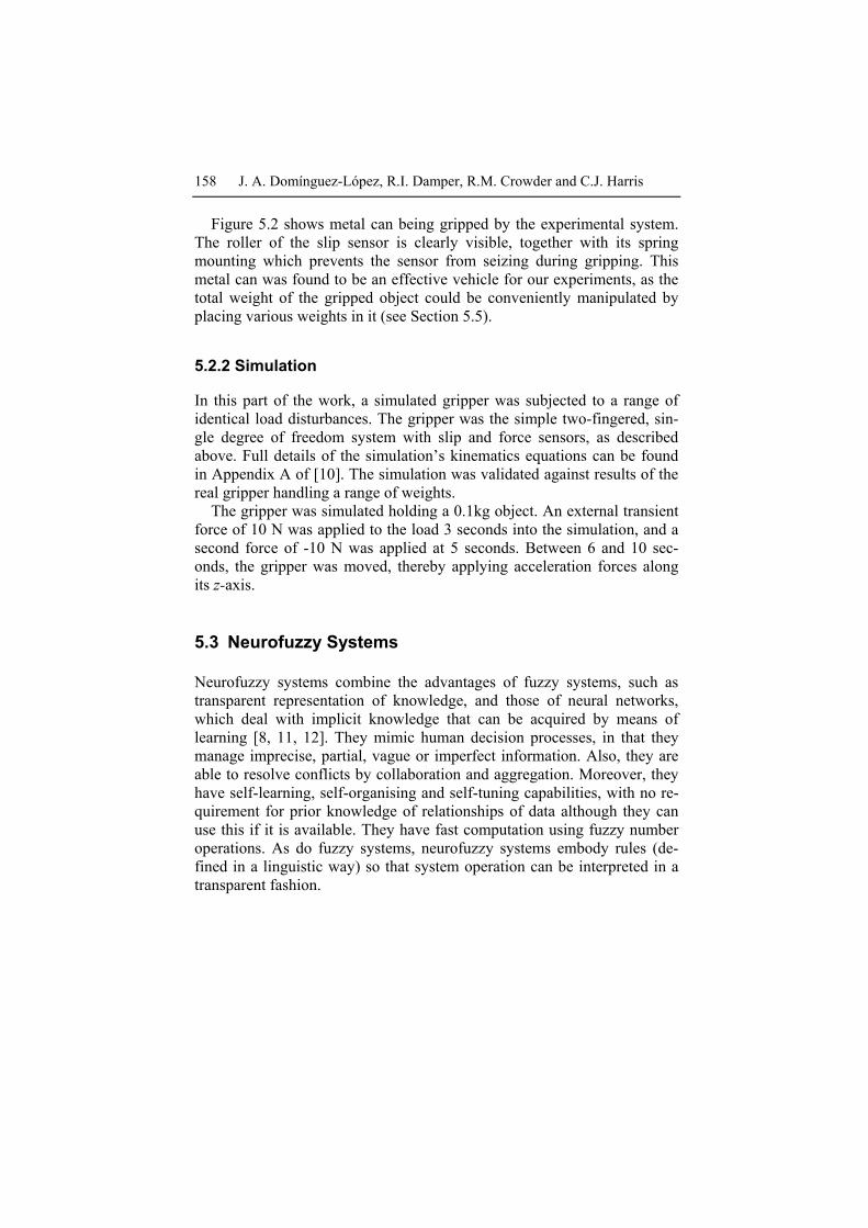
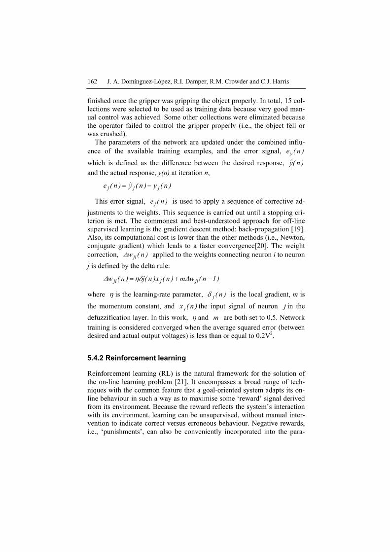
Figure 5.3 Architecture of a typical neurofuzzy system. The number of rules is given by ii NP ∏= where i is the number of inputs and Ni is the number of an-tecedent fuzzy sets for input i while M is the number of consequent fuzzy sets. In addition, ∑= i iNQ and ∑= −
=1i0k kNR
Figure 5.3 shows the implementation of a neurofuzzy system as a feed forward network with three layers, namely: the fuzzification layer, the fuzzy rule layer and defuzzification layer. The mapping between the first two layers is nonlinear and linear between the last two layers [13]. The fuzzification layer consists of two components: the measurements ix , which are the input signals from the system under control and the envi-ronment, and the computation of the antecedent membership function value, )x( iAij
µ termed the grade of membership. The fuzzy rule layer
then calculates the rule firing strength, which indicates how well the condi-tions in the antecedent are satisfied. An input x fires a rule to a degree,
]1,0[w∈ . The calculation of the rule firing strength is performed using the membership function values for fuzzy sets used in the rule antecedent.
160 J. A. Domínguez-López, R.I. Damper, R.M. Crowder and C.J. Harris
It is dependent on how the antecedents are combined (i.e., using AND, OR). The product combiner is the fuzzy implication method, used because it preserves the original shape of the fuzzy set and it is differentiable. Fi-nally, the defuzzification layer converts the values delivered by the fired rules at the previous layer into analogue output values. Centre of sums (CoS) and centre of gravity (CoG) are the most often used defuzzification techniques. The CoS approach has some advantages over CoG; in particu-lar, CoS is faster because it is simpler to program [14]. The resulting de-fuzzified values are combined by some averaging method (denoted OR in Figure 5.3).
The antecedent and consequent weights ( kia and mnb respectively), and the rule confidences )w( ij can be updated. In fact, there are two main possibilities for learning: adjust these weights, or adjust the shape of the membership functions. The latter can be achieved only if the membership functions are parametric. In this work, we fix all antecedent and conse-quent values, and membership functions; only rule confidences are learned.
5.4 Training Methods
A neurofuzzy controller is able to learn about its environment through a process of adjusting its weights and bias levels. The learning paradigms used to tune the network weights are commonly divided into three main classes: supervised, unsupervised and reinforcement [15]. These learning algorithms can be used individually or in conjunction[16, 17]. In super-vised learning, a teacher gives the system a representative collection of in-put-output examples constituting knowledge of the problem environment. For unsupervised learning, no such specification is made of which output should be associated with particular inputs. Rather, the system bases its free-parameter updating on some quality measure of the representation of the learning goal. Reinforcement learning (RL) is a broad class of machine learning techniques in which the ‘teacher’ is replaced by an evaluative sig-nal (or signals) derived from the environment. Hence, it is eminently suit-able for on-line robot learning applications in which continuous interaction with the environment is all-important. Furthermore, RL is fully automatic, doing away with the need for intervention of an expert (the ‘teacher’) to provide a suitable training dataset. The evaluative (or reinforcement) sig-nals do not specify what the correct answer should be, since this is un-known. Rather, they specify whether the system output is right or wrong, as well as (possibly) providing a scalar indication of the degree of correct-
5 Intelligent Neurofuzzy Control of a Robotic Gripper 161
ness. This evaluative signal is often couched in terms of a reward or a pun-ishment, for being right or wrong respectively. Because there is no explicit provision of a correct answer by a ‘teacher’, we take RL to be distinct from supervised learning—although some researchers do treat it as supervised “because the network does, after all, get some feedback from the environ-ment” [18, p188].
In our work, we have used both supervised and reinforcement learning to produce neurofuzzy controllers for the gripper. We have also used a hy-brid of the two. Hence, we have a total of three learning systems: off-line supervised learning, reinforcement on-line learning and a hybrid of super-vised and reinforcement on-line learning.
5.4.1 Supervised learning
In supervised learning, knowledge of the problem environment is repre-sented by a set of input-output examples—the training dataset. The task of the learning algorithm is to adjust the system parameters in response to the given inputs so as to reproduce the desired output [15, p63]. To achieve high system performance, the training data must be consistent and com-plete. This is an obvious shortcoming of the supervised learning approach for our problem. In the real environment, we will not be able to anticipate all conditions which will be met, so it is not possible to guarantee com-pleteness.
To collect the training data, a simple C program was written to control the gripper manually using several keys of the PC keyboard. Six keys were used for a fixed applied motor voltage (i.e., -5, 0, 1.5, 2.7, 3.9, 5V) and four to increase/decrease the applied voltage by 0.1V or 0.25V. The opera-tor (the first author), using personnel judgment and the current object status (e.g., gripper or not, crushed, etc.), manually increased/decreased the applied voltage so the gripper could grasp the object properly (i.e. fast, stable, with minimum finger force and without allowing the object to fall). An extra (stop) key was included to allow the operator to pause and rethink the action to be taken to be taken as well as to check the object status. The data collected during the stopped time was not used for training because they are not actually part of the control action.
Several trials were carried out to obtain several collections of training data. Every trial started with the gripper fingers completely opened. The object used was an empty can with uneven surface and variable weight. The weight was varied using cans with different mass (i.e., 50, 125 and 210 grams). During the manual control, several disturbances of different magnitude were applied on the object to induce slip. Each experiment was
162 J. A. Domínguez-López, R.I. Damper, R.M. Crowder and C.J. Harris
finished once the gripper was gripping the object properly. In total, 15 col-lections were selected to be used as training data because very good man-ual control was achieved. Some other collections were eliminated because the operator failed to control the gripper properly (i.e., the object fell or was crushed).
The parameters of the network are updated under the combined influ-ence of the available training examples, and the error signal, )n(ey
which is defined as the difference between the desired response, )n(y and the actual response, y(n) at iteration n,
)n(y)n(y)n(e jjj −=
This error signal, )n(e j is used to apply a sequence of corrective ad-justments to the weights. This sequence is carried out until a stopping cri-terion is met. The commonest and best-understood approach for off-line supervised learning is the gradient descent method: back-propagation [19]. Also, its computational cost is lower than the other methods (i.e., Newton, conjugate gradient) which leads to a faster convergence[20]. The weight correction, )n(w ji∆ applied to the weights connecting neuron i to neuron j is defined by the delta rule:
)1n(wm)n(x)n(j)n(w jijji −+= ∆ηδ∆
where η is the learning-rate parameter, )n(jδ is the local gradient, m is the momentum constant, and )n(x j the input signal of neuron j in the defuzzification layer. In this work, η and m are both set to 0.5. Network training is considered converged when the average squared error (between desired and actual output voltages) is less than or equal to 0.2V2.
5.4.2 Reinforcement learning
Reinforcement learning (RL) is the natural framework for the solution of the on-line learning problem [21]. It encompasses a broad range of tech-niques with the common feature that a goal-oriented system adapts its on-line behaviour in such a way as to maximise some ‘reward’ signal derived from its environment. Because the reward reflects the system’s interaction with its environment, learning can be unsupervised, without manual inter-vention to indicate correct versus erroneous behaviour. Negative rewards, i.e., ‘punishments’, can also be conveniently incorporated into the para-
5 Intelligent Neurofuzzy Control of a Robotic Gripper 163
digm. In view of its generality and on-line nature, RL has found wide ap-plication in robotics and autonomous system studies (e.g., [22-24]).
In many formulations of RL, the system is supposed to decide the best action to select based on its current state. When this step is repeated, the problem is known as a Markov decision process [25]. A finite Markov de-cision process (MDP) is defined by the state and action sets, and by the one-step dynamics of the environment. The components of an MDP are:
• a set of states S; • a set of actions A; • a reinforcement function ℜ→× AS:R ; and • a state transition function ∏→× )S(AS:T where ∏ )S( is a prob-
ability distribution over the set S.
At each decision point, the controller has to select an action based on the environmental information (i.e., state). After performing the action ia the system receives an immediate reinforcement, ir . The action taken affects the subsequent state, 1is + . The probability distribution of the reinforce-ment tr and the subsequent state 1is + .depends only on the starting state
1is + and the taken action ia . The objective of the system is to maximise the sum of discounted rewards [26, 27]. The reinforcement at time t is given by:
∑=∞
=+
0i1i
ii rr γ
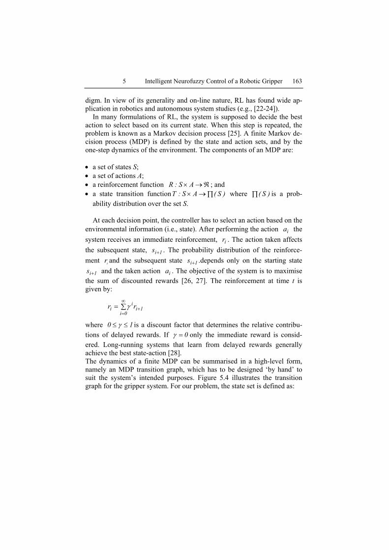
where 10 ≤≤ γ is a discount factor that determines the relative contribu-tions of delayed rewards. If 0=γ only the immediate reward is consid-ered. Long-running systems that learn from delayed rewards generally achieve the best state-action [28]. The dynamics of a finite MDP can be summarised in a high-level form, namely an MDP transition graph, which has to be designed ‘by hand’ to suit the system’s intended purposes. Figure 5.4 illustrates the transition graph for the gripper system. For our problem, the state set is defined as:
164 J. A. Domínguez-López, R.I. Damper, R.M. Crowder and C.J. Harris
S2crushing
S0not_touching
S1slipping
S3OK
grip
grip
grip
grip
release
release
release( )crushingt12, +−β
( )crushingt110,1 +−
161 −β+α− ),(
)t1(10, crushing+α
)t1(2),(1 slip+−β+α−
( )slipt15, +−β
( )OKt12,1 +−α−
GRIPR,α RELEASER,α
161 −β+α− ),(
1,α
0,1 α−
161 −β− ,
( )slipt110, +−β
( )OKt15, +−β
)t1(10, slip+α
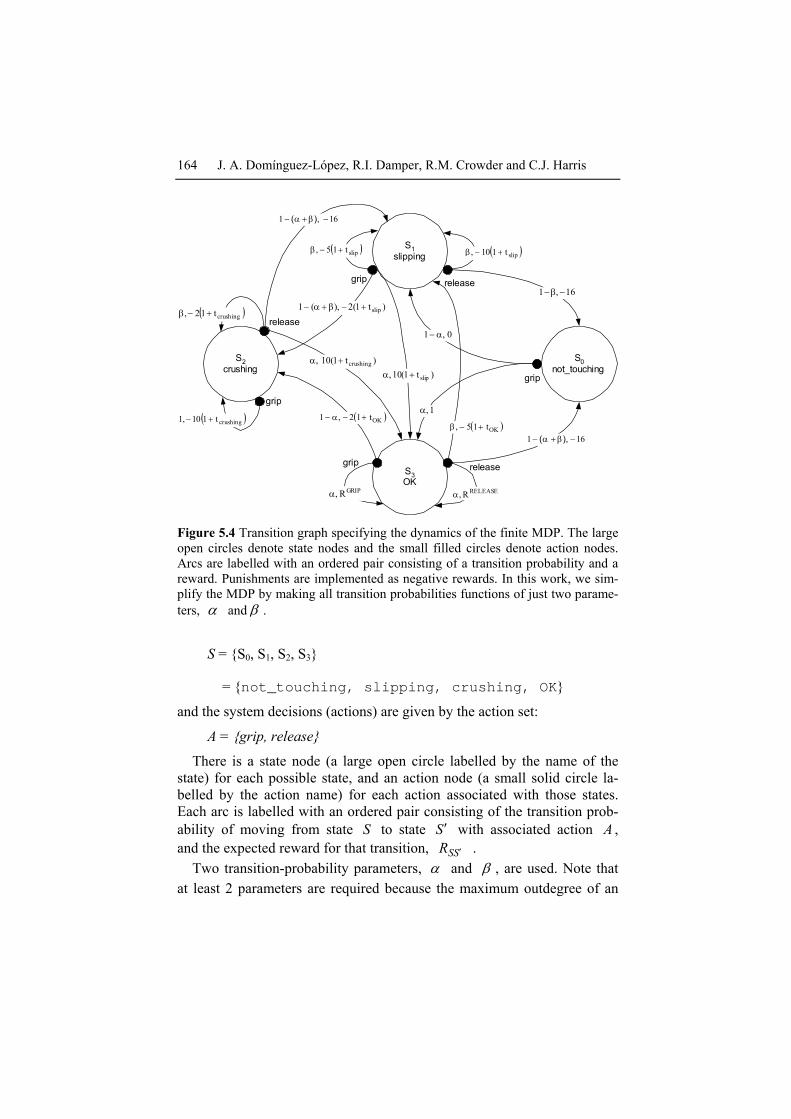
Figure 5.4 Transition graph specifying the dynamics of the finite MDP. The large open circles denote state nodes and the small filled circles denote action nodes. Arcs are labelled with an ordered pair consisting of a transition probability and a reward. Punishments are implemented as negative rewards. In this work, we sim-plify the MDP by making all transition probabilities functions of just two parame-ters, α and β .
S = {S0, S1, S2, S3}
= {not_touching, slipping, crushing, OK}
and the system decisions (actions) are given by the action set:
A = {grip, release}
There is a state node (a large open circle labelled by the name of the state) for each possible state, and an action node (a small solid circle la-belled by the action name) for each action associated with those states. Each arc is labelled with an ordered pair consisting of the transition prob-ability of moving from state S to state S ′ with associated action A , and the expected reward for that transition, SSR ′ .
Two transition-probability parameters, α and β , are used. Note that at least 2 parameters are required because the maximum outdegree of an
5 Intelligent Neurofuzzy Control of a Robotic Gripper 165
action node is 3, and 1 degree of freedom is fixed since the transition prob-abilities must sum to 1. Accordingly, α is set relatively high, as it de-notes a transition probability into a desired state (i.e., OK), while β is set relatively low. In many cases, but not all, β indicates a transition prob-ability into a undesirable state (i.e., slipping or crushing). In some cases, the transition probability into these states will be )(1 βα +− , so a further requirement is that 1<+ βα to ensure that these transition prob-abilities do not vanish. In this work, α and β have been set by trial and error to 0.85 and 0.12, respectively.
Rewards and punishments are either fixed, or made to depend upon the time spent in the originating state for that transition. This is to increase the rewards and punishments if the system keeps in a good or bad state-action, respectively. Rewards are attached to transitions into the OK state. Punish-ments are attached to transitions into the undesirable (slipping, crushing and not_touching) states. Time-dependent rewards have the effect of increasing the reward for moving to the OK state according to the length of time spent in an undesirable state, and conversely for pun-ishments. Both time-dependent and fixed rewards/punishments have been set empirically. Transitions with a -16 punishment are included in the MDP specification for completeness; it is envisaged that they would never occur in the trained network. When the object is being satisfactorily gripped, i.e., the system remains in the state OK for t
OK, the rewards for the
two associated actions grip and release are:
)t1(2500
F2500cRR OKRELEASE
SSGRIP
SS 3333+
−==
where tOK
is the time without both slipping and crushing, F is the applied force and c is a constant empirically set equal to 20 in this work. With this scheme, the rate of increase of the reward decreases as the applied force approaches its upper limit of 2500, corresponding physically to 2500 mN.
There are three fundamental classes of methods that tackle the rein-forcement learning problem: dynamic programming (DP), Monte Carlo methods and temporal difference (TD) learning. TD methods are based on learning the difference(s) between temporally-successive predictions. As TD learning combines characteristics of dynamic programming (i.e., pol-icy evaluation, value iteration) and Monte Carlo methods, it can approxi-mate the value function using update estimates from other learned esti-mates, like those found from dynamic programming. Also, like Monte Carlo methods, TD methods can learn from experience following a policy without the dynamics of the environment. Accordingly, TD has some ad-
166 J. A. Domínguez-López, R.I. Damper, R.M. Crowder and C.J. Harris
vantages over the other methods [21]. The most important ones are: TD methods do not require a model of the environment, rewards and next-state probability distribution while DP methods do; TD methods can be imple-mented in an on-line fashion while Monte Carlo methods can not.
Policy
ValueFunction
Environment
ActionStateCritic
Actor
TDError
Reward
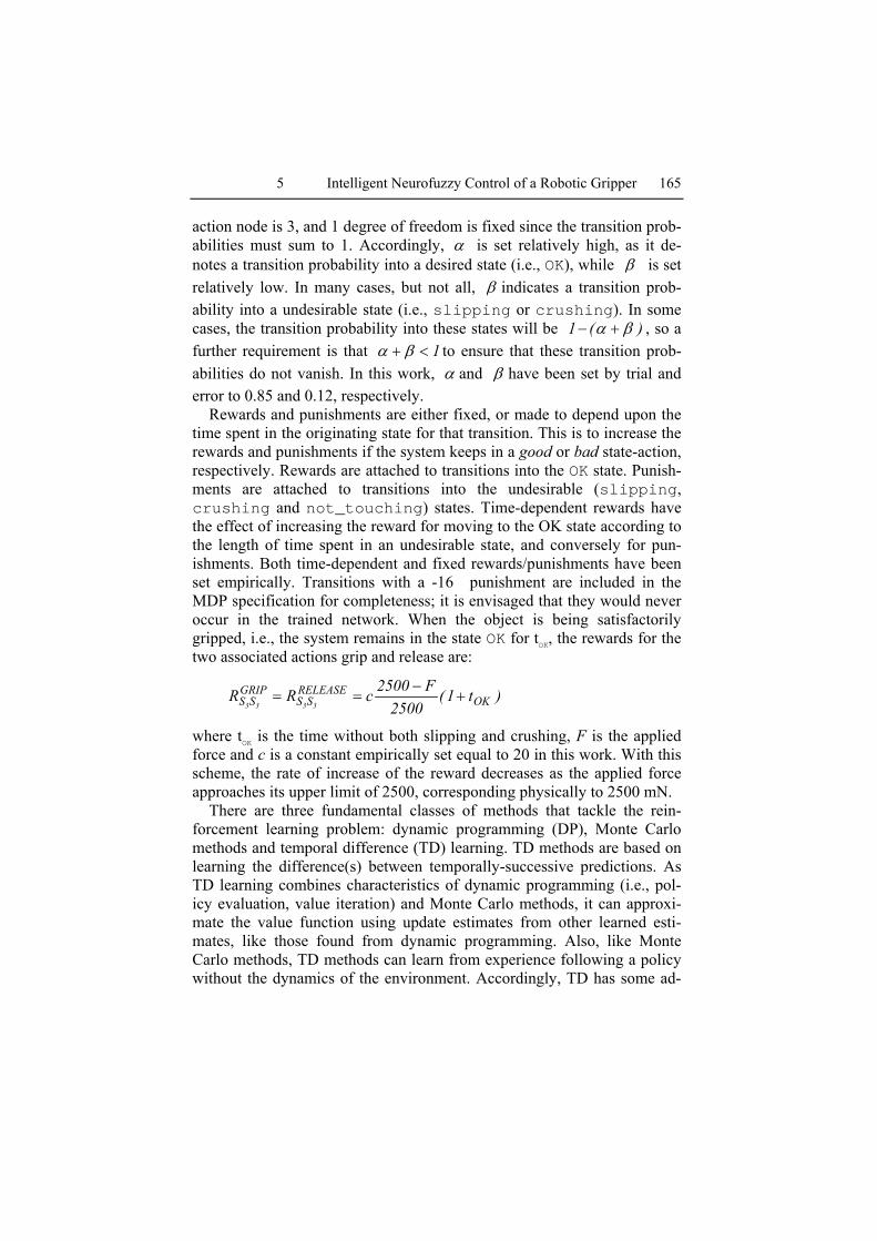
Figure 5.5 Block diagram of the actor-critic reinforcement learning system.
In this work, we have used an actor-critic framework. Actor-critic methods are temporal difference learning methods [29]. To solve the pre-diction problem, TD methods compute the state-value function using the experience of following a policy (i.e., the mapping between states and ac-tions). At the next time step, based on the obtained reward or punishment, the estimated value function for a given policy is updated. Actor-critic methods have two separate memories in order to represent the policy inde-pendently of the value function. This leads to the following most important advantages of actor-critic methods over other TD techniques: minimal computation required to select actions and its ability to learn an explicitly stochastic policy, allowing the optimal probability of selecting appropriate actions to be learned [21, p153]. Figure 5.5 shows the architecture of the actor-critic method. The policy structure is the actor and the estimated value function is the critic. The former selects actions and the latter criti-cises those actions. This criticism has the form of an ‘internal’ (TD-error) signal to drive the learning process.
5 Intelligent Neurofuzzy Control of a Robotic Gripper 167
Action Selection
Network(neurofuzzy controller)
Action EvaluationNetwork
(neural predictor)
Stochastic ActionModifier
Motor Voltage
Sampleandhold
v(t - 1)
Environment
failure(t-1)
state(t - 1)
Weight Updating
)t(r
)t(f ′
)t(s
)t(f
)t(state
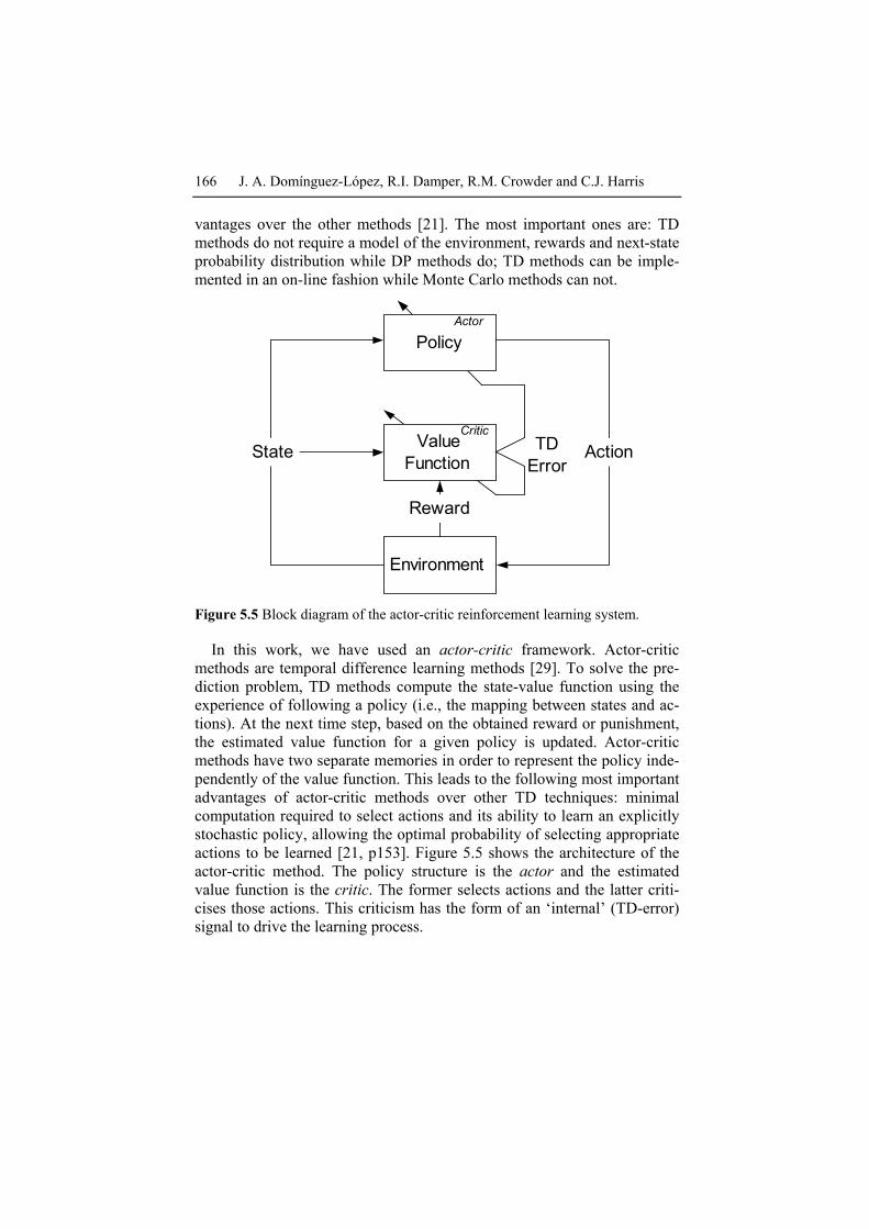
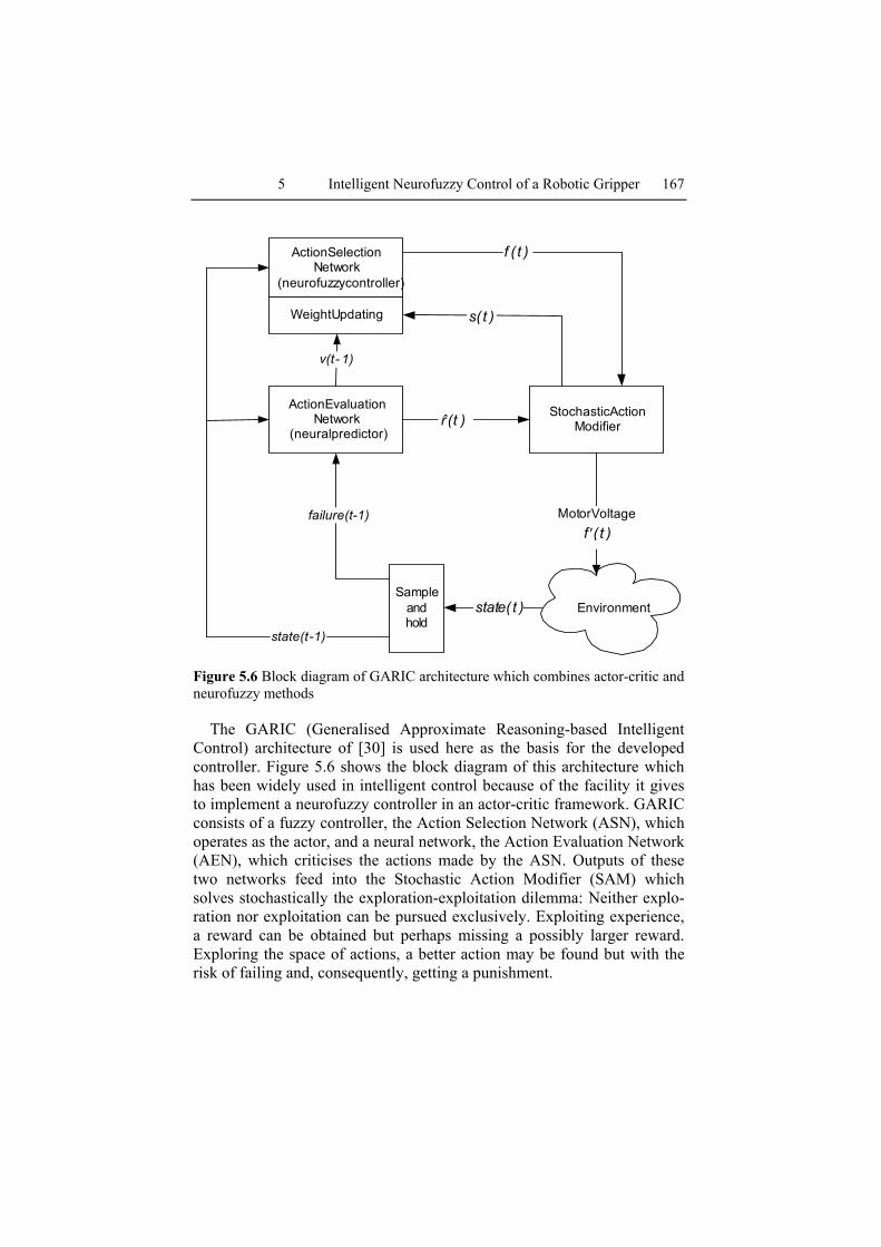
Figure 5.6 Block diagram of GARIC architecture which combines actor-critic and neurofuzzy methods
The GARIC (Generalised Approximate Reasoning-based Intelligent Control) architecture of [30] is used here as the basis for the developed controller. Figure 5.6 shows the block diagram of this architecture which has been widely used in intelligent control because of the facility it gives to implement a neurofuzzy controller in an actor-critic framework. GARIC consists of a fuzzy controller, the Action Selection Network (ASN), which operates as the actor, and a neural network, the Action Evaluation Network (AEN), which criticises the actions made by the ASN. Outputs of these two networks feed into the Stochastic Action Modifier (SAM) which solves stochastically the exploration-exploitation dilemma: Neither explo-ration nor exploitation can be pursued exclusively. Exploiting experience, a reward can be obtained but perhaps missing a possibly larger reward. Exploring the space of actions, a better action may be found but with the risk of failing and, consequently, getting a punishment.
168 J. A. Domínguez-López, R.I. Damper, R.M. Crowder and C.J. Harris
Action Selection Network
The Action Selection Network is the fuzzy controller that performs all the control operations. The fuzzy controller is expanded into a neurofuzzy controller so its parameters can be updated according to the signal received from the Action Evaluation Network. The employment of a (neuro)fuzzy network as critic gives transparency to the system. That is, the behaviour of the physical system is described by a set of easily-interpreted linguistic rules. These can then be used to understand and validate the process under control, or to modify it.
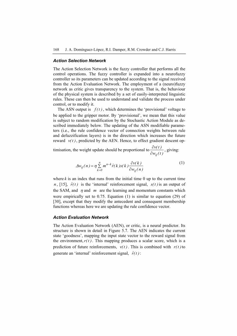
The ASN output is )t(f , which determines the ‘provisional’ voltage to be applied to the gripper motor. By ‘provisional’, we mean that this value is subject to random modification by the Stochastic Action Module as de-scribed immediately below. The updating of the ASN modifiable parame-ters (i.e., the rule confidence vector of connection weights between rule and defuzzification layers) is in the direction which increases the future reward )t(v , predicted by the AEN. Hence, to effect gradient descent op-
timisation, the weight update should be proportional to)t(w
)t(v
ij∂∂ , giving:
∑∂∂
==
−n
0k ij
knij )n(w
)k(v)k(s)k(rm)n(w η∆ (1)
where k is an index that runs from the initial time 0 up to the current time n , [15], )t(r is the ‘internal’ reinforcement signal, )t(s is an output of the SAM, and η and m are the learning and momentum constants which were empirically set to 0.75. Equation (1) is similar to equation (29) of [30], except that they modify the antecedent and consequent membership functions whereas here we are updating the rule confidence vector.
Action Evaluation Network
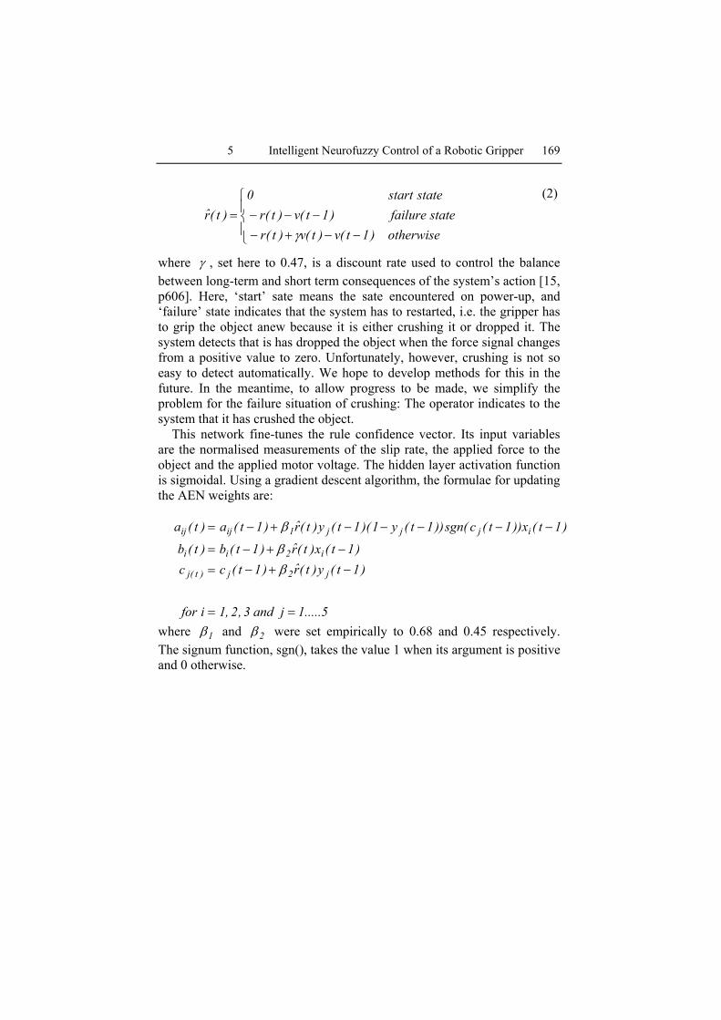
The Action Evaluation Network (AEN), or critic, is a neural predictor. Its structure is shown in detail in Figure 5.7. The AEN indicates the current state ‘goodness’, mapping the input state vector to the reward signal from the environment, )t(r . This mapping produces a scalar score, which is a prediction of future reinforcements, )t(v . This is combined with )t(r to generate an ‘internal’ reinforcement signal, )t(r :
5 Intelligent Neurofuzzy Control of a Robotic Gripper 169
−−+−−−−=
otherwise)1t(v)t(v)t(rstatefailure)1t(v)t(r
statestart0)t(r
γ
(2)
where γ , set here to 0.47, is a discount rate used to control the balance between long-term and short term consequences of the system’s action [15, p606]. Here, ‘start’ sate means the sate encountered on power-up, and ‘failure’ state indicates that the system has to restarted, i.e. the gripper has to grip the object anew because it is either crushing it or dropped it. The system detects that is has dropped the object when the force signal changes from a positive value to zero. Unfortunately, however, crushing is not so easy to detect automatically. We hope to develop methods for this in the future. In the meantime, to allow progress to be made, we simplify the problem for the failure situation of crushing: The operator indicates to the system that it has crushed the object.
This network fine-tunes the rule confidence vector. Its input variables are the normalised measurements of the slip rate, the applied force to the object and the applied motor voltage. The hidden layer activation function is sigmoidal. Using a gradient descent algorithm, the formulae for updating the AEN weights are:
5.....1jand3,2,1ifor
)1t(y)t(r)1t(cc)1t(x)t(r)1t(b)t(b
)1t(x))1t(csgn())1t(y1)(1t(y)t(r)1t(a)t(a
j2j)t(j
i2ii
ijjj1ijij
==
−+−=
−+−=
−−−−−+−=
ββ
β
where 1β and 2β were set empirically to 0.68 and 0.45 respectively. The signum function, sgn(), takes the value 1 when its argument is positive and 0 otherwise.
170 J. A. Domínguez-López, R.I. Damper, R.M. Crowder and C.J. Harris
y2
y1
y3
y4
y5
Markov Desision Process
a11
a35
a12
v(t)
b2
b1
b3
r(t)
)t(r
System State
x1Slip
x3Motor
Voltage
x2Force
c3
c5
c4
c2
c1
∑
CombinationalRules
Equation 2
Failure Signal
Figure 5.7. The Action Evaluation Network consists of a neural network predict-ing future reward, )t(v , which is combined with the reward signal, )t(r , from the environment to produce an ‘internal’ reward signal, )t(r , as described by equation (2).
Stochastic Action Modifier
The Stochastic Action Modifier gives a stochastic deviation to the output of the ASN, so the system can have a better exploration of the state space and a better generalisation ability [16]. The numerical amount of deviation, which is used as a learning factor for ASN, is given by,
)1t(r
**'
e)t(y)t(y)t(s
−−−
=
where instead of using )t(y* as output, the control action applied to the
system is )t(y*' a Gaussian random variable with mean )t(y* and stan-
dard deviation )1t(re −− This leads to the action having a large deviation when the last taken action was bad, and conversely when the action was good.
5 Intelligent Neurofuzzy Control of a Robotic Gripper 171
Weight Updating
LabelledTraining Data
Supervised LearningNetwork
Action SelectionNetwork
(neurofuzzy controller)
Action EvaluationNetwork
(neural predictor)
Stochastic ActionModifier
Motor Voltage
Sampleandhold
v(t-1)
Environment
Weight Updating
)t(r
)t(f ′
)t(f
)t(s
)1t(failure −
)t(state 1−
)t(state
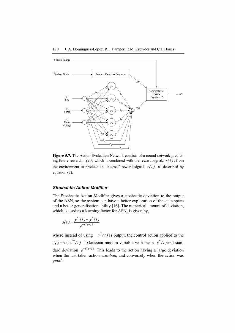
Figure 5.8 Block diagram of the hybrid supervised/reinforcement system in which a Supervised Learning Network (SLN), trained on pre-labelled data, is added to the basic GARIC architecture
5.4.3 Hybrid learning
Looking to have a faster adaptation to environmental changes, we have implemented a hybrid learning approach which uses both supervised and reinforcement learning. The combination of these two training algorithms allows the system to have a faster adaptation [16]. The hybrid approach has not only the characteristic of self-adaptation but the ability to make best use of knowledge (i.e., pre-labelled training data) should they exist. The proposed hybrid algorithm is also based on the GARIC architecture. An extra neurofuzzy block, the supervised learning network (SLN), is added to the original structure (Figure 5.8). The SLN is a neurofuzzy con-troller which is trained in non-real time with (supervised) back-propagation. When new training data are available, the SLN is retrained without stopping the system execution; then it sends a parameter updating
172 J. A. Domínguez-López, R.I. Damper, R.M. Crowder and C.J. Harris
signal to the action selection network. The ASN parameters can now be updated if appropriate.
As new training data become available during system operation (see be-low), the SLN loads the rule-weight vector from the ASN and starts its (re)training, which continues until the stop criterion is reached (average er-ror less than or equal to 0.2V2, see Section 5.4.1). The information loaded (i.e, rule confidence vector) from the ASN is utilised as a priori knowl-edge by the SLN. Once the SLN training has finished, the new rule weight vector is sent back to the ASN. Elements of the confidence vector (i.e., weights) are transferred from the SLN to the ASN only if the difference between them is lower than or equal to 5%:
iSLNi
ASNi
SLNi
ASNi
SLNi
ASNi
w95.0wthen
)w05.1w()w95.0w(if
∀←
<∧>
(3)
where i counts over all corresponding ASN and SLN weights. Neurofuzzy techniques do not require a mathematical model of the sys-
tem under control. The major disadvantage of the lack of this model is the impossibility to derive a stability criterion. Consequently, the use of a 5% threshold as in equation (3) was proposed as an attempt to minimise the risk of system instability. This allows the hybrid system to ‘ignore’ pre-labelled data if they were inconsistent with current-encountered conditions (given by the AEN). The value of 5% was set empirically, although the system was not especially sensitive to this value. For instance, during a se-ries of tests with the value set to 10%, the system still maintained correct operation.
5.5 Results with Real Gripper
To validate the performance of the various learning systems, various ex-periments have been undertaken to compare the resulting controllers used in conjunction with the simple, low-cost, two-finger end effector (Section 5.2.1). The information provided by the force and slip sensors forms the inputs to the neurofuzzy controller, and the output is the applied motor voltage. Inputs are normalised to the range [0, 1].
Experiments were carried out with a range of weights placed in one of the metal cans (Figure 5.2). Hence, the weight of the object was different from that utilised in collecting the labelled training data (when the cans were empty). This is intended to test the ability of neurofuzzy control to
5 Intelligent Neurofuzzy Control of a Robotic Gripper 173
maintain correct operation robustly in the face of conditions not previously encountered. In addition, information concerning the object to be gripped and the end effector itself were never given to the control system. To recap, three experimental conditions were studied:
i. off-line supervised learning with back-propagation training; ii. on-line reinforcement learning; iii. hybrid of supervised and reinforcement learning.
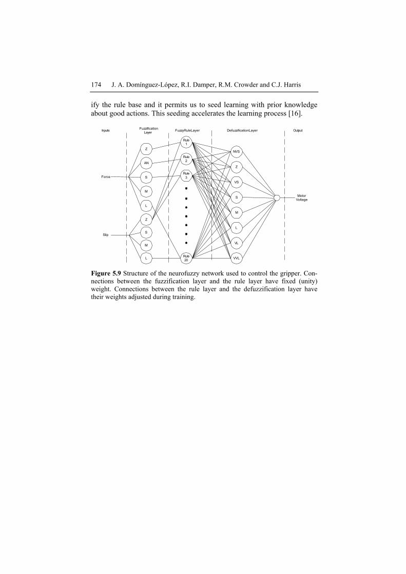
In (i), we learn ‘from scratch’ by back-propagation using the neurofuzzy
network depicted in Figure 5.9. The linguistic variables used for the term sets are simply value magnitude components: Zero (Z), Very Small (VS), Small (S), Medium (M) and Large (L) for the fuzzy set slip while for the applied force they are Z, S, M and L. The output fuzzy set (motor voltage) has the set members Negative Very Small (NVS), Z, Very Small (VS), S, M, L, Very Large (VL) and Very Very Large (VVL). This set has more members so as to have a smoother output. In (ii), reinforcement learning is seeded with the rule base obtained in (i), to see if RL can improve back-propagation. The ASN of the GARIC architecture is a neurofuzzy network with structure as in Figure. 5.9. In (iii), RL is again seeded with the rule base from (i), and when RL discovers a ‘good’ action, this is added to the training set for background supervised learning. Specifically, when t
ok
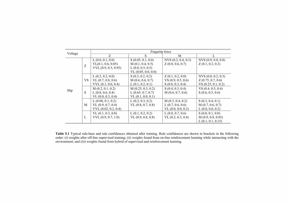
reaches 3 seconds, it is assumed that gripping has been successful; and in-put-output data recorded over this interval are concatenated onto the la-belled training set. In this way, we hope to ensure that such good actions do not get ‘forgotten’ as on-line learning proceeds. Typical rule-base and rule confidences achieved after training are presented in tabular form in Table 5.1. In the table, each rule has three confidence values correspond-ing to conditions (i), (ii) and (iii) above. We choose to show typical results because the precise findings depend on things like the initial start points for the weights [31], the action of the Stochastic Action Modifier in the re-inforcement and hybrid learning systems, the precise weights in the metal can, and the length of time that the system runs for. Nonetheless, in spite of these complications, some useful generalisations can be drawn.
One of the virtues of neurofuzzy systems is that the learned rules are transparent so that it should be fairly obvious to the reader what these mean and how they effect control of the object. For example, if the slip is large and the fingertip force is small, it means that we are in danger of dropping the object and the force must be increased rapidly by making the motor voltage very large. As can be seen in the table, this particular rule has a high confidence for all three learning strategies (0.9, 0.8 and 0.8 for (i), (ii) and (iii) respectively). Network transparency allows the user to ver-
174 J. A. Domínguez-López, R.I. Damper, R.M. Crowder and C.J. Harris
ify the rule base and it permits us to seed learning with prior knowledge about good actions. This seeding accelerates the learning process [16].
MotorVoltage
VVLRule20L
NVS
Force
Slip
FuzzificationLayer Fuzzy Rule Layer Defuzzification Layer OutputInputs
Rule2
Rule3
Rule1
M
S
Z
L
M
S
AN
Z
VL
L
M
S
VS
Z
Figure 5.9 Structure of the neurofuzzy network used to control the gripper. Con-nections between the fuzzification layer and the rule layer have fixed (unity) weight. Connections between the rule layer and the defuzzification layer have their weights adjusted during training.
Fingertip force Voltage
Z S M L
Z
L (0.0, 0.1, 0.0) VL(0.1, 0.6, 0.05) VVL (0.9, 0.3, 0.95)
S (0.05, 0.1, 0.0) M (0.1, 0.4, 0.5) L (0.8, 0.5, 0.5) VL (0.05, 0.0, 0.0)
NVS (0.2, 0.4, 0.3) Z (0.8, 0.6, 0.7)
NVS (0.9, 0.8, 0.8) Z (0.1, 0.2, 0.2)
VSL (0.2, 0.2, 0.0) VL (0.7, 0.8, 0.6) VVL (0.1, 0.0, 0.4)
S (0.3, 0.2, 0.2) M (0.6, 0.6, 0.7) L (0.1, 0.2, 0.1)
Z (0.1, 0.2, 0.0) VS (0.9, 0.5, 0.6) S (0.0, 0.3, 0.4)
NVS (0.0, 0.2, 0.3) Z (0.75, 0.7, 0.6) VS (0.25, 0.1, 0.2)
S M (0.2, 0.1, 0.2) L (0.8, 0.6, 0.4) VL (0.0, 0.3, 0.4)
M (0.25, 0.3, 0.2) L (0.65, 0.7, 0.7) VL (0.1, 0.0, 0.1)
S (0.4, 0.3, 0.4) M (0.6, 0.7, 0.6)
VS (0.4, 0.5, 0.4) S (0.6, 0.5, 0.6)
M L (0.08, 0.1, 0.2) VL (0.9, 0.7, 0.4) VVL (0.02, 0.2, 0.4)
L (0.2, 0.3, 0.2) VL (0.8, 0.7, 0.8)
M (0.3, 0.4, 0.2) L (0.7, 0.6, 0.6) VL (0.0, 0.0, 0.2)
S (0.3, 0.4, 0.1) M (0.7, 0.6, 0.7) L (0.0, 0.0, 0.2)
Slip
L VL (0.1, 0.3, 0.0) VVL (0.9, 0.7, 1.0)
L (0.1, 0.2, 0.2) VL (0.9, 0.8, 0.8)
L (0.8, 0.7, 0.6) VL (0.2, 0.3, 0.4)
S (0.0, 0.1, 0.0) M (0.9, 0.8, 0.85) L (0.1, 0.1, 0.15)
Table 5.1 Typical rule-base and rule confidences obtained after training. Rule confidences are shown in brackets in the following order: (i) weights after off-line supervised training; (ii) weights found from on-line reinforcement learning while interacting with the environment; and (iii) weights found from hybrid of supervised and reinforcement learning.
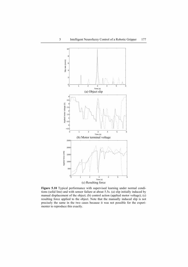
To answer the question of which system is the best, the three learning methods were tested under two conditions: normal (i.e., same conditions as they were trained for) and environmental change (i.e., simulated sensor failure). The first condition evaluates the systems’ learning speed while the second one tests their robustness to unanticipated operating conditions. Performances were investigated by manually introducing several distur-bances of various intensities acting on the object to induce slip. For all the tests, the experimenter must attempt to reproduce the same pattern of man-ual disturbance inducing slip at different times so that different conditions can be compared. This is clearly not possible to do precisely. (It was aided by using an audible beep from the computer to prompt the investigator and to act as a timing reference.) To allow easy comparison of these slightly different experimental conditions, we have aligned plots on the major in-duced disturbance, somewhat arbitrarily fixed at 3 s.
The solid line of Figure 5.10 shows typical performance of the super-vised learning system under normal conditions; the dashed line shows op-eration when a sensor failure is introduced at about 5.5 s. The system learned how to perform under normal conditions but when there is a change in the environment, it is unable to adapt to this change unless re-trained with new data which include the change.
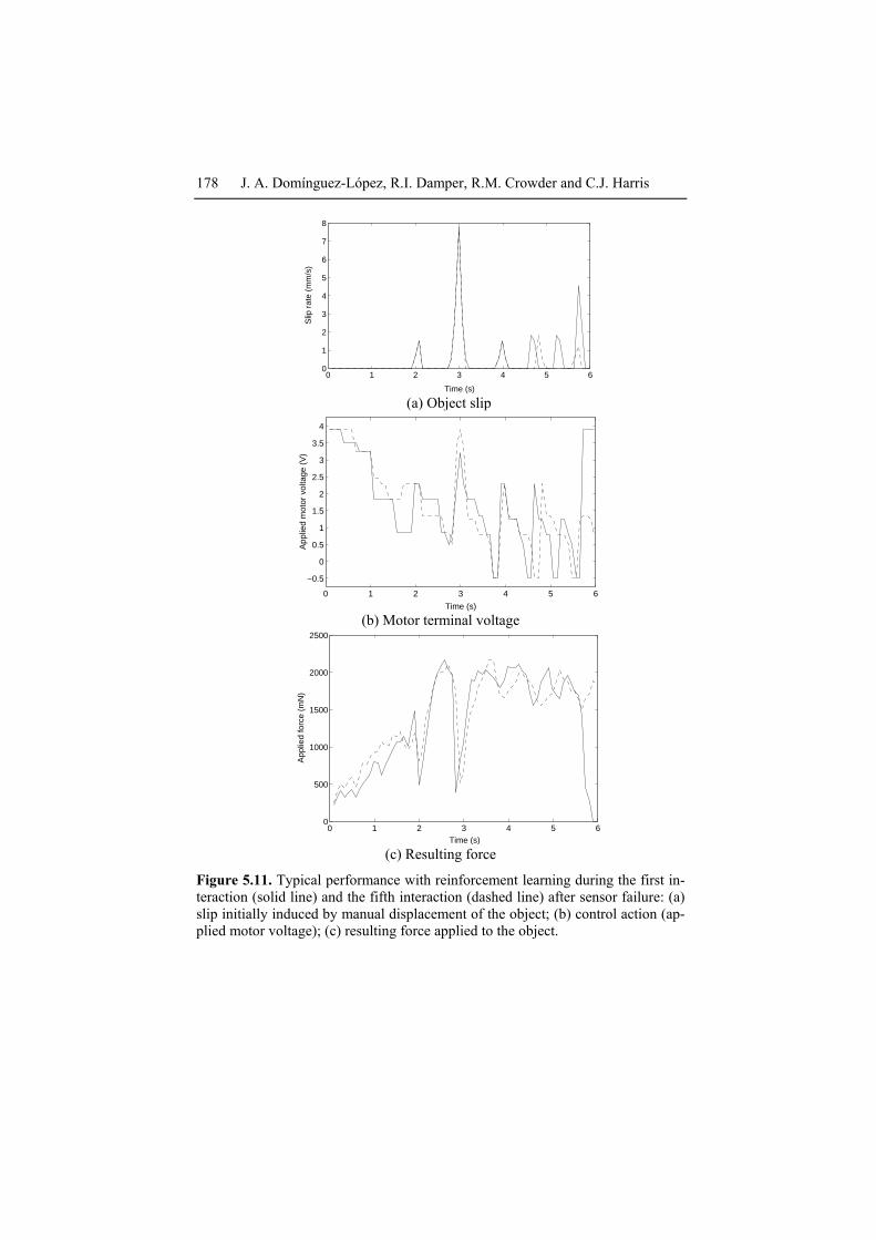
Figure 5.11 shows the performance of the system trained with rein-forcement learning during the first interaction (solid) and fifth interaction (dashed) after the simulated sensor failure. To simulate continuous on-line learning but in a way which allows comparison of results as training pro-ceeds, we broke each complete RL trial into a series of ‘interactions’. After each such interaction, lasting approximately 6 s, the rule base and rule con-fidence vector obtained were then used as the start point for reinforcement learning for the next interaction. (Note that the first interaction after a sen-sor failure is actually the second interaction in real terms.) Simulated sen-sor failure were introduced at approximately 5.5 s during the (absolute) first interaction. As can be seen, during the first interaction following a failure, the object dropped just before 6 s. There is a rapid fall off of resul-tant force (Figure 5.11(b)) while the control action (end effector motor voltage) saturates (Figure 5.11(c)). The control action is ineffective be-cause the object is no longer present, having been dropped. By the fifth in-teraction after a failure, however, an appropriate control strategy has been learned. Effective force is applied to the object using a moderate motor voltage. The controller learns that it is not applying as much force as it ‘thinks’. This result demonstrates the effectiveness of on-line reinforce-ment learning, as the system is able to perform a successful grip in re-sponse to an environmental change and manually-induced slip.
5 Intelligent Neurofuzzy Control of a Robotic Gripper 177
0 1 2 3 4 5 60
2
4
6
8
10
Time (s)
Slip
rat
e (m
m/s
)
(a) Object slip
0 1 2 3 4 5 6
−0.5
0
0.5
1
1.5
2
2.5
3
3.5
4
Time (s)
App
lied
mot
or v
olta
ge (
V)
(b) Motor terminal voltage
0 1 2 3 4 5 60
500
1000
1500
2000
2500
Time (s)
App
lied
forc
e (m
N)
(c) Resulting force
Figure 5.10 Typical performance with supervised learning under normal condi-tions (solid line) and with sensor failure at about 5.5s. (a) slip initially induced by manual displacement of the object; (b) control action (applied motor voltage); (c) resulting force applied to the object. Note that the manually induced slip is not precisely the same in the two cases because it was not possible for the experi-menter to reproduce this exactly.
178 J. A. Domínguez-López, R.I. Damper, R.M. Crowder and C.J. Harris
0 1 2 3 4 5 60
1
2
3
4
5
6
7
8
Time (s)
Slip
rat
e (m
m/s
)
(a) Object slip
0 1 2 3 4 5 6
−0.5
0
0.5
1
1.5
2
2.5
3
3.5
4
Time (s)
App
lied
mot
or v
olta
ge (
V)
(b) Motor terminal voltage
0 1 2 3 4 5 60
500
1000
1500
2000
2500
Time (s)
App
lied
forc
e (m
N)
(c) Resulting force
Figure 5.11. Typical performance with reinforcement learning during the first in-teraction (solid line) and the fifth interaction (dashed line) after sensor failure: (a) slip initially induced by manual displacement of the object; (b) control action (ap-plied motor voltage); (c) resulting force applied to the object.
5 Intelligent Neurofuzzy Control of a Robotic Gripper 179
0 1 2 3 4 5 6 7 80
2
4
6
8
10
Time (s)
Slip
rat
e (m
m/s
)
(a) Object slip
0 1 2 3 4 5 6 7 8
0
1
2
3
4
Time (s)
App
lied
mot
or v
olta
ge (
V)
(b) Motor terminal voltage
0 1 2 3 4 5 6 7 80
500
1000
1500
2000
Time (s)
App
lied
forc
e (m
N)
(c) Applied force
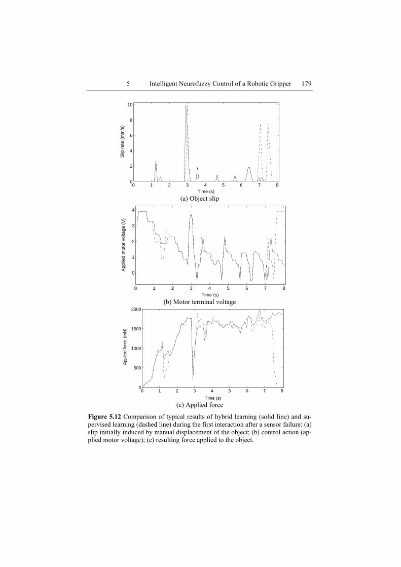
Figure 5.12 Comparison of typical results of hybrid learning (solid line) and su-pervised learning (dashed line) during the first interaction after a sensor failure: (a) slip initially induced by manual displacement of the object; (b) control action (ap-plied motor voltage); (c) resulting force applied to the object.
180 J. A. Domínguez-López, R.I. Damper, R.M. Crowder and C.J. Harris
Figure 5.12 shows the performance of the hybrid trained system during the first interaction after a failure (solid line) and compares it with the per-formance of the system trained with supervised learning (dashed line). Note that the latter result is identical to that shown by the full line in Fig-ure 5.10. It is clear that the hybrid trained system is able to adapt itself to this disturbance where the supervised trained system is unable to adapt and fails, dropping the object.
The important conclusions drawn from this work on the real gripper are as follows. For the system to have on-line adaptation to unanticipated con-ditions, its training has to be unsupervised. (For our purposes, we count reinforcement learning as unsupervised.) The use of a priori knowledge to seed the initial rules helps to achieve quicker neurofuzzy learning. The use of knowledge about good control actions, gained during system operation, can also improve on-line learning. For all these reasons, a hybrid of unsupervised and reinforcement learning should be superior to the other methods. This superiority is obvious when the hybrid is compared against off-line supervised learning.
5.6 Simulation of Gripper and Six Degree of Freedom Robot
Thus far, the gripper studied has been very simple, with a two-input, one-output control action and a single degree of freedom. We wished to con-sider more complex and practical setups, such as when the gripper is mounted on a full six degree of freedom robot and has more sensor capa-bilities (e.g., accelerometer). A particular reason for this is that neurofuzzy systems are known to be subject to the well-known curse of dimensionality [32, 33] whereby required system resources grow exponentially with prob-lem size (e.g., the number of sensor inputs). To avoid the considerable cost of studying these issues with a real robot, this part of the work was done by software simulation.
A simulation of a 6 DOF robot was developed to have the effects of the robot movements and orientation on the gripping process of the end effec-tor and to avoid the considerable cost of building the full manipulator. The experiments reported here were undertaken under two conditions: external forces acting on the object (with the end effector stationary), and vertical end effector acceleration.
Four approaches are evaluated for the gripper controller with the pres-ence of end effector acceleration:
5 Intelligent Neurofuzzy Control of a Robotic Gripper 181
i. traditional approach without accelerometer; ii. traditional approach with accelerometer;
iii. approach with accelerometer and hierarchical modelling; iv. hierarchical approach with acceleration control.
These are described in the following sections. As the situation studied is virtual, we do not have any labelled data suitable for supervised training. Hence, the four approaches are trained using reinforcement learning. The Markov decision process is the only component which remains identical for all the approaches. The action selection network and the action evalua-tion network are modified to reflect the new input.
5.6.1 Approach without acceleration feedback
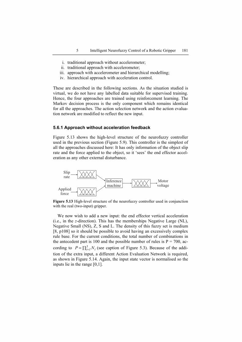
Figure 5.13 shows the high-level structure of the neurofuzzy controller used in the previous section (Figure 5.9). This controller is the simplest of all the approaches discussed here: It has only information of the object slip rate and the force applied to the object, so it ‘sees’ the end effector accel-eration as any other external disturbance.
Inferencemachine
Appliedforce
Sliprate
Motorvoltage
Figure 5.13 High-level structure of the neurofuzzy controller used in conjunction with the real (two-input) gripper.
We now wish to add a new input: the end effector vertical acceleration (i.e., in the z-direction). This has the memberships Negative Large (NL), Negative Small (NS), Z, S and L. The density of this fuzzy set is medium [8, p108] so it should be possible to avoid having an excessively complex rule base. For the current conditions, the total number of combinations in the antecedent part is 100 and the possible number of rules is P = 700, ac-cording to ∏= =
31i iNP (see caption of Figure 5.3). Because of the addi-
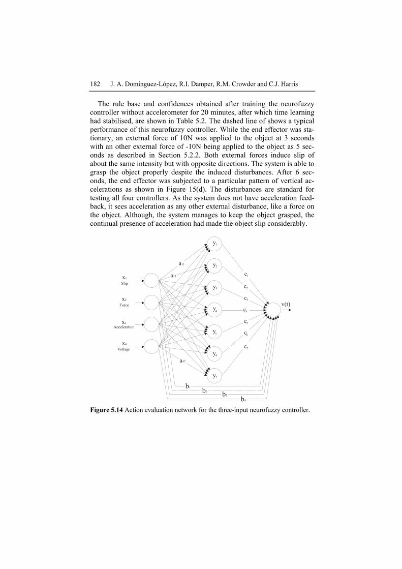
tion of the extra input, a different Action Evaluation Network is required, as shown in Figure 5.14. Again, the input state vector is normalised so the inputs lie in the range [0,1].
182 J. A. Domínguez-López, R.I. Damper, R.M. Crowder and C.J. Harris
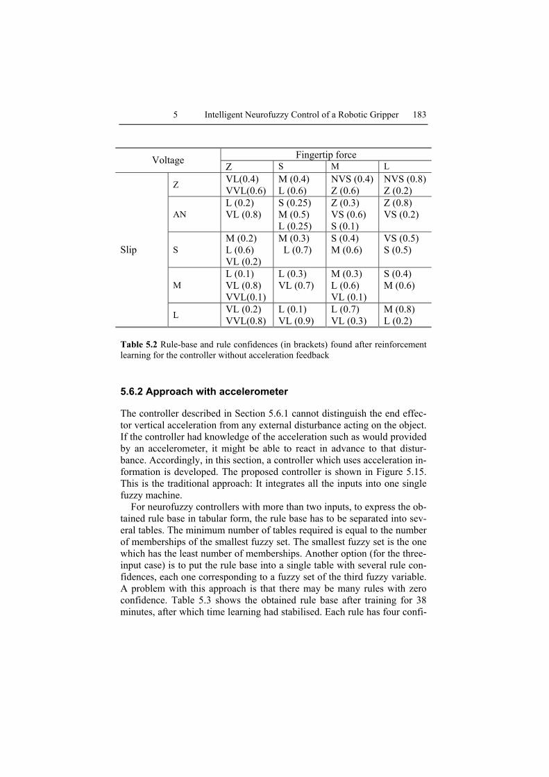
The rule base and confidences obtained after training the neurofuzzy controller without accelerometer for 20 minutes, after which time learning had stabilised, are shown in Table 5.2. The dashed line of shows a typical performance of this neurofuzzy controller. While the end effector was sta-tionary, an external force of 10N was applied to the object at 3 seconds with an other external force of -10N being applied to the object as 5 sec-onds as described in Section 5.2.2. Both external forces induce slip of about the same intensity but with opposite directions. The system is able to grasp the object properly despite the induced disturbances. After 6 sec-onds, the end effector was subjected to a particular pattern of vertical ac-celerations as shown in Figure 15(d). The disturbances are standard for testing all four controllers. As the system does not have acceleration feed-back, it sees acceleration as any other external disturbance, like a force on the object. Although, the system manages to keep the object grasped, the continual presence of acceleration had made the object slip considerably.
v(t)x2
Acceleration
Force
Voltage
x3
x4
x1
Slip
1y
2y
3y
4y
5y
6y
7y
a12
a11
a47
c1
c2
c3
c4
c6
c5
c7
b2
b1
b3
b4 Figure 5.14 Action evaluation network for the three-input neurofuzzy controller.
5 Intelligent Neurofuzzy Control of a Robotic Gripper 183
Fingertip force Voltage
Z S M L
Z VL(0.4) VVL(0.6)
M (0.4) L (0.6)
NVS (0.4)Z (0.6)
NVS (0.8) Z (0.2)
AN L (0.2) VL (0.8)
S (0.25) M (0.5) L (0.25)
Z (0.3) VS (0.6) S (0.1)
Z (0.8) VS (0.2)
S M (0.2) L (0.6) VL (0.2)
M (0.3) L (0.7)
S (0.4) M (0.6)
VS (0.5) S (0.5)
M L (0.1) VL (0.8) VVL(0.1)
L (0.3) VL (0.7)
M (0.3) L (0.6) VL (0.1)
S (0.4) M (0.6)
Slip
L VL (0.2) VVL(0.8)
L (0.1) VL (0.9)
L (0.7) VL (0.3)
M (0.8) L (0.2)
Table 5.2 Rule-base and rule confidences (in brackets) found after reinforcement learning for the controller without acceleration feedback
5.6.2 Approach with accelerometer
The controller described in Section 5.6.1 cannot distinguish the end effec-tor vertical acceleration from any external disturbance acting on the object. If the controller had knowledge of the acceleration such as would provided by an accelerometer, it might be able to react in advance to that distur-bance. Accordingly, in this section, a controller which uses acceleration in-formation is developed. The proposed controller is shown in Figure 5.15. This is the traditional approach: It integrates all the inputs into one single fuzzy machine.
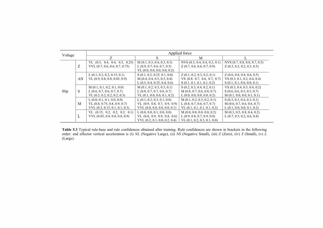
For neurofuzzy controllers with more than two inputs, to express the ob-tained rule base in tabular form, the rule base has to be separated into sev-eral tables. The minimum number of tables required is equal to the number of memberships of the smallest fuzzy set. The smallest fuzzy set is the one which has the least number of memberships. Another option (for the three-input case) is to put the rule base into a single table with several rule con-fidences, each one corresponding to a fuzzy set of the third fuzzy variable. A problem with this approach is that there may be many rules with zero confidence. Table 5.3 shows the obtained rule base after training for 38 minutes, after which time learning had stabilised. Each rule has four confi-
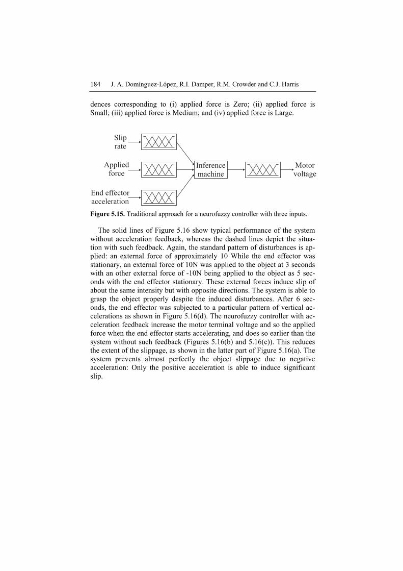
184 J. A. Domínguez-López, R.I. Damper, R.M. Crowder and C.J. Harris
dences corresponding to (i) applied force is Zero; (ii) applied force is Small; (iii) applied force is Medium; and (iv) applied force is Large.
Inferencemachine
Appliedforce
Sliprate
Motorvoltage
End effectoracceleration Figure 5.15. Traditional approach for a neurofuzzy controller with three inputs.
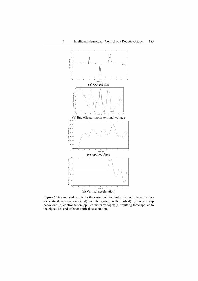
The solid lines of Figure 5.16 show typical performance of the system without acceleration feedback, whereas the dashed lines depict the situa-tion with such feedback. Again, the standard pattern of disturbances is ap-plied: an external force of approximately 10 While the end effector was stationary, an external force of 10N was applied to the object at 3 seconds with an other external force of -10N being applied to the object as 5 sec-onds with the end effector stationary. These external forces induce slip of about the same intensity but with opposite directions. The system is able to grasp the object properly despite the induced disturbances. After 6 sec-onds, the end effector was subjected to a particular pattern of vertical ac-celerations as shown in Figure 5.16(d). The neurofuzzy controller with ac-celeration feedback increase the motor terminal voltage and so the applied force when the end effector starts accelerating, and does so earlier than the system without such feedback (Figures 5.16(b) and 5.16(c)). This reduces the extent of the slippage, as shown in the latter part of Figure 5.16(a). The system prevents almost perfectly the object slippage due to negative acceleration: Only the positive acceleration is able to induce significant slip.
5 Intelligent Neurofuzzy Control of a Robotic Gripper 185
0 1 2 3 4 5 6 7 8 9 10−8
−6
−4
−2
0
2
4
6
8
Time (s)
Slip
rat
e (c
m/s
)
(a) Object slip
0 1 2 3 4 5 6 7 8 9 10−2
−1
0
1
2
3
4
Time (s)
App
lied
mot
or v
olta
ge (
V)
(b) End effector motor terminal voltage
0 1 2 3 4 5 6 7 8 9 100
500
1000
1500
2000
2500
3000
3500
Time (s)
App
lied
forc
e (m
N)
(c) Applied force
0 1 2 3 4 5 6 7 8 9 10−30
−20
−10
0
10
20
Time (s)
End
effe
ctor
ver
tical
acc
eler
atio
n (m
/s2 )
(d) Vertical acceleration]
Figure 5.16 Simulated results for the system without information of the end effec-tor vertical acceleration (solid) and the system with (dashed): (a) object slip behaviour; (b) control action (applied motor voltage); (c) resulting force applied to the object; (d) end effector vertical acceleration.
Applied force Voltage Z S M L
Z VL (0.3, 0.4, 0.4, 0.3, 0.25) VVL (0.7, 0.6, 0.6, 0.7, 0.75)
M (0.1, 0.3, 0.4, 0.3, 0.3) L (0.9, 0.7, 0.6, 0.7, 0.5) VL (0.0, 0.0, 0.0, 0.0, 0.2)
NVS (0.3, 0.4, 0.4, 0.3, 0.1) Z (0.7, 0.6, 0.6, 0.7, 0.9)
NVS (0.7, 0.8, 0.8, 0.7, 0.5) Z (0.3, 0.2, 0.2, 0.3, 0.5)
AN L (0.1, 0.2, 0.2, 0.15, 0.1) VL (0.9, 0.8, 0.8, 0.85, 0.9)
S (0.1, 0.2, 0.25, 0.1, 0.0) M (0.4, 0.4, 0.5, 0.5, 0.4) L (0.5, 0.4, 0.25, 0.4, 0.6)
Z (0.1, 0.2, 0.3, 0.2, 0.1) VS (0.8, 0.7, 0.6, 0.7, 0.7) S (0.1, 0.1, 0.1, 0.1, 0.2)
Z (0.6, 0.8, 0.8, 0.6, 0.5) VS (0.3, 0.1, 0.2, 0.4, 0.4) S (0.1, 0.1, 0.0, 0.0, 0.1)
S M (0.1, 0.1, 0.2, 0.1, 0.0) L (0.6, 0.7, 0.6, 0.7, 0.7) VL (0.3, 0.2, 0.2, 0.2, 0.3)
M (0.1, 0.2, 0.3, 0.3, 0.1) L (0.8, 0.7, 0.7, 0.6, 0.7) VL (0.1, 0.0, 0.0, 0.1, 0.2)
S (0.2, 0.3, 0.4, 0.2, 0.1) M (0.8, 0.7, 0.6, 0.8, 0.7) L (0.0, 0.0, 0.0, 0.0, 0.2)
VS (0.3, 0.4, 0.5, 0.4, 0.2) S (0.6, 0.6, 0.5, 0.5, 0.7) M (0.1, 0.0, 0.0, 0.1, 0.1)
M L (0.0, 0.1, 0.1, 0.0, 0.0) VL (0.8, 0.75, 0.8, 0.9, 0.7) VVL (0.2, 0.15, 0.1, 0.1, 0.3)
L (0.1, 0.2, 0.3, 0.1, 0.0) VL (0.9, 0.8, 0.7, 0.9, 0.9) VVL (0.0, 0.0, 0.0, 0.0, 0.1)
M (0.1, 0.2, 0.3, 0.2, 0.1) L (0.8, 0.7, 0.6, 0.7, 0.7) VL (0.1, 0.1, 0.1, 0.1, 0.2)
S (0.3, 0.3, 0.4, 0.3, 0.1) M (0.6, 0.7, 0.6, 0.6, 0.7) L (0.1, 0.0, 0.0, 0.1, 0.2)
Slip
L VL (0.15, 0.2, 0.2, 0.2, 0.1) VVL (0.85, 0.8, 0.8, 0.8, 0.9)
L (0.0, 0.0, 0.1, 0.0, 0.0) VL (0.8, 0.9, 0.9, 0.8, 0.6) VVL (0.2, 0.1, 0.0, 0.2, 0.4)
M (0.0, 0.0, 0.0, 0.0, 0.2) L (0.9, 0.8, 0.7, 0.9, 0.8) VL (0.1, 0.2, 0.3, 0.1, 0.0)
M (0.3, 0.5, 0.8, 0.4, 0.2) L (0.7, 0.5, 0.2, 0.6, 0.8)
Table 5.3 Typical rule-base and rule confidences obtained after training. Rule confidences are shown in brackets in the following order: end effector vertical acceleration is (i) NL (Negative Large), (ii) NS (Negative Small), (iii) Z (Zero), (iv) S (Small), (v) L (Large).
Comparing the performances of the system with and without acceleration feedback, we conclude the following. When there is no end effector accel-eration, both systems perform similarly. In the presence of end effector ac-celeration, the system with acceleration feedback is able to eliminate or re-duce the slippage. However, this improvement has come at the price of having now 700 possible rules whereas before there were only 140 possi-ble rules. So, there is a trade-off between simplicity of the system and a better performance. Nevertheless, this application involving three inputs is still considered a low-dimensional problem [8, p108]; the 700 possible rules demand modest memory and processing time. Accordingly, the me-chanical response is not affected by undue processing delay.
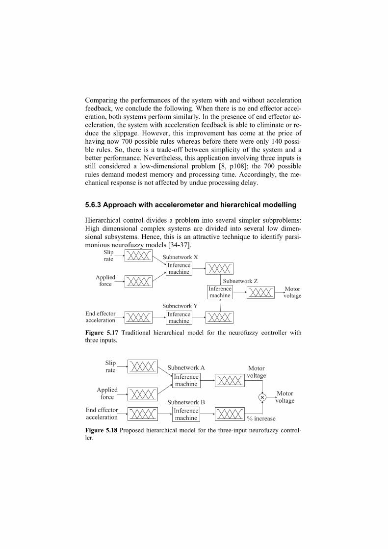
5.6.3 Approach with accelerometer and hierarchical modelling
Hierarchical control divides a problem into several simpler subproblems: High dimensional complex systems are divided into several low dimen-sional subsystems. Hence, this is an attractive technique to identify parsi-monious neurofuzzy models [34-37].
Inferencemachine
Appliedforce
Sliprate
Motorvoltage
End effectoracceleration
Inferencemachine
Inferencemachine
Subnetwork X
Subnetwork Y
Subnetwork Z
Figure 5.17 Traditional hierarchical model for the neurofuzzy controller with three inputs.
Inferencemachine
Appliedforce
Sliprate
Motorvoltage
End effectoracceleration
Inferencemachine
+
Motorvoltage
% increase
Subnetwork B
Subnetwork A
Figure 5.18 Proposed hierarchical model for the three-input neurofuzzy control-ler.
188 J. A. Domínguez-López, R.I. Damper, R.M. Crowder and C.J. Harris
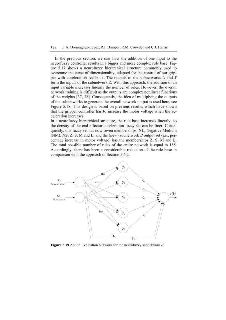
In the previous section, we saw how the addition of one input to the neurofuzzy controller results in a bigger and more complex rule base. Fig-ure 5.17 shows a neurofuzzy hierarchical structure commonly used to overcome the curse of dimensionality, adapted for the control of our grip-per with acceleration feedback. The outputs of the subnetworks X and Y form the inputs of the subnetwork Z. With this approach, the addition of an input variable increases linearly the number of rules. However, the overall network training is difficult as the outputs are complex nonlinear functions of the weights [37, 38]. Consequently, the idea of multiplying the outputs of the subnetworks to generate the overall network output is used here, see Figure 5.18. This design is based on previous results, which have shown that the gripper controller has to increase the motor voltage when the ac-celeration increases. In a neurofuzzy hierarchical structure, the rule base increases linearly, so the density of the end effector acceleration fuzzy set can be finer. Conse-quently, this fuzzy set has now seven memberships: NL, Negative Medium (NM), NS, Z, S, M and L, and the (new) subnetwork B output set (i.e., per-centage increase in motor voltage) has the memberships Z, S, M and L. The total possible number of rules of the entire network is equal to 188. Accordingly, there has been a considerable reduction of the rule base in comparison with the approach of Section 5.6.2.
v(t)
x1
Acceleration
% increase
x2
1y
2y
3y
4y
5y
c1
c2
c3
c4
c5
b1
b2
a12
a11
a25
Figure 5.19 Action Evaluation Network for the neurofuzzy subnetwork B.
5 Intelligent Neurofuzzy Control of a Robotic Gripper 189
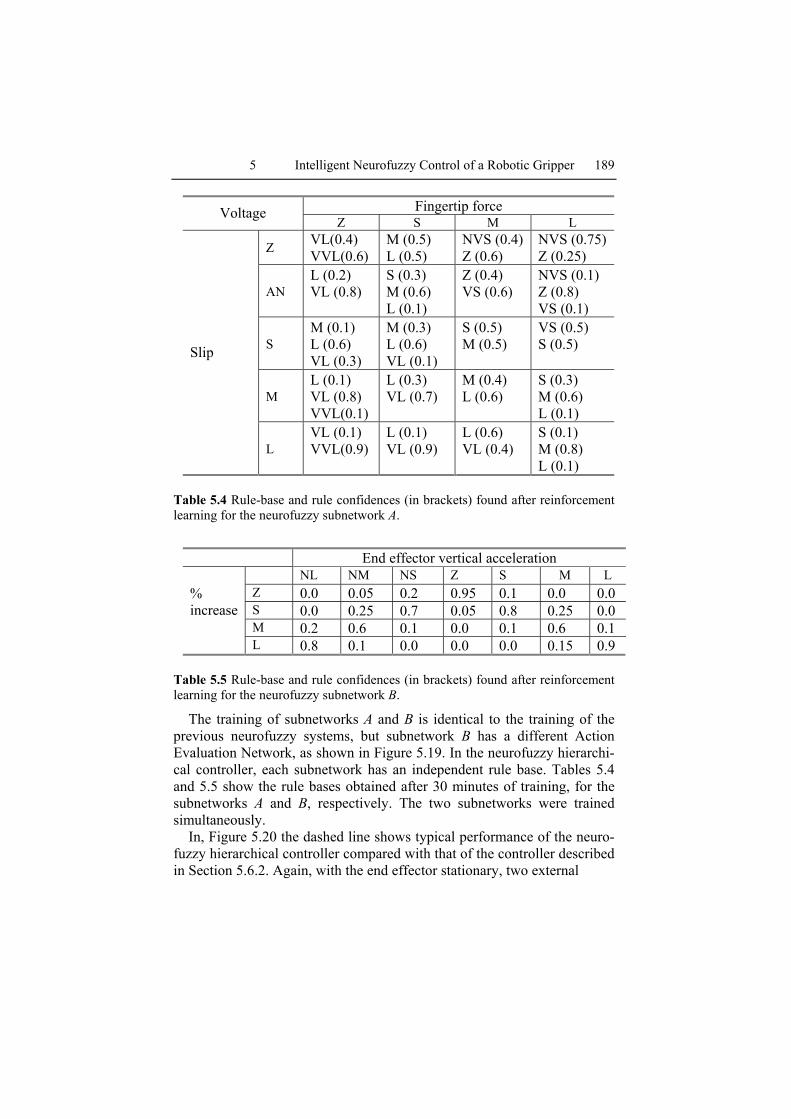
Fingertip force Voltage Z S M L
Z VL(0.4) VVL(0.6)
M (0.5) L (0.5)
NVS (0.4)Z (0.6)
NVS (0.75) Z (0.25)
AN L (0.2) VL (0.8)
S (0.3) M (0.6) L (0.1)
Z (0.4) VS (0.6)
NVS (0.1) Z (0.8) VS (0.1)
S M (0.1) L (0.6) VL (0.3)
M (0.3) L (0.6) VL (0.1)
S (0.5) M (0.5)
VS (0.5) S (0.5)
M L (0.1) VL (0.8) VVL(0.1)
L (0.3) VL (0.7)
M (0.4) L (0.6)
S (0.3) M (0.6) L (0.1)
Slip
L VL (0.1) VVL(0.9)
L (0.1) VL (0.9)
L (0.6) VL (0.4)
S (0.1) M (0.8) L (0.1)
Table 5.4 Rule-base and rule confidences (in brackets) found after reinforcement learning for the neurofuzzy subnetwork A.
End effector vertical acceleration NL NM NS Z S M L
Z 0.0 0.05 0.2 0.95 0.1 0.0 0.0 S 0.0 0.25 0.7 0.05 0.8 0.25 0.0 M 0.2 0.6 0.1 0.0 0.1 0.6 0.1
% increase
L 0.8 0.1 0.0 0.0 0.0 0.15 0.9
Table 5.5 Rule-base and rule confidences (in brackets) found after reinforcement learning for the neurofuzzy subnetwork B.
The training of subnetworks A and B is identical to the training of the previous neurofuzzy systems, but subnetwork B has a different Action Evaluation Network, as shown in Figure 5.19. In the neurofuzzy hierarchi-cal controller, each subnetwork has an independent rule base. Tables 5.4 and 5.5 show the rule bases obtained after 30 minutes of training, for the subnetworks A and B, respectively. The two subnetworks were trained simultaneously.
In, Figure 5.20 the dashed line shows typical performance of the neuro-fuzzy hierarchical controller compared with that of the controller described in Section 5.6.2. Again, with the end effector stationary, two external
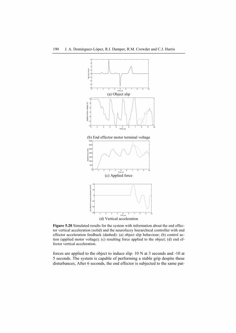
190 J. A. Domínguez-López, R.I. Damper, R.M. Crowder and C.J. Harris
0 1 2 3 4 5 6 7 8 9 10−8
−6
−4
−2
0
2
4
6
8
Time (s)
Slip
rat
e (c
m/s
)
(a) Object slip
0 1 2 3 4 5 6 7 8 9 10−2
−1
0
1
2
3
4
Time (s)
App
lied
mot
or v
olta
ge (
V)
(b) End effector motor terminal voltage
0 1 2 3 4 5 6 7 8 9 100
500
1000
1500
2000
2500
3000
3500
Time (s)
App
lied
forc
e (m
N)
(c) Applied force
0 1 2 3 4 5 6 7 8 9 10−30
−20
−10
0
10
20
Time (s)
End
effe
ctor
ver
tical
acc
eler
atio
n (m
/s2 )
(d) Vertical acceleration
Figure 5.20 Simulated results for the system with information about the end effec-tor vertical acceleration (solid) and the neurofuzzy hierarchical controller with end effector acceleration feedback (dashed): (a) object slip behaviour; (b) control ac-tion (applied motor voltage); (c) resulting force applied to the object; (d) end ef-fector vertical acceleration.
forces are applied to the object to induce slip: 10 N at 3 seconds and -10 at 5 seconds. The system is capable of performing a stable grip despite these disturbances, After 6 seconds, the end effector is subjected to the same pat-
5 Intelligent Neurofuzzy Control of a Robotic Gripper 191
tern of acceleration as before. Again, this controller is able to mange excel-lently the negative acceleration, and reduce slippage for the positive accel-eration. The neurofuzzy hierarchical system was not only able to reduce the number of rules but also give a slight improvement in the system per-formance.
Neurofuzzycontroller
(2)
Neurofuzzycontroller
(1)Applied force
Slip rate
AccelerationApplied motor
voltage (gripper)
Suggestedend effectoracceleration
Limiter
Desiredend effectoracceleration
maximumacceleration| |
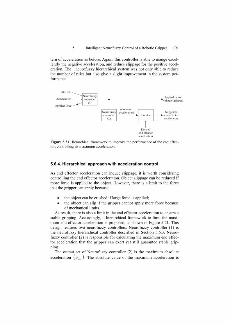
Figure 5.21 Hierarchical framework to improve the performance of the end effec-tor, controlling its maximum acceleration.
5.6.4. Hierarchical approach with acceleration control
As end effector acceleration can induce slippage, it is worth considering controlling the end effector acceleration. Object slippage can be reduced if more force is applied to the object. However, there is a limit to the force that the gripper can apply because:
• the object can be crushed if large force is applied; • the object can slip if the gripper cannot apply more force because
of mechanical limits. As result, there is also a limit in the end effector acceleration to ensure a
stable gripping. Accordingly, a hierarchical framework to limit the maxi-mum end effector acceleration is proposed, as shown in Figure 5.21. This design features two neurofuzzy controllers. Neurofuzzy controller (1) is the neurofuzzy hierarchical controller described in Section 5.6.3. Neuro-fuzzy controller (2) is responsible for calculating the maximum end effec-tor acceleration that the gripper can exert yet still guarantee stable grip-ping.
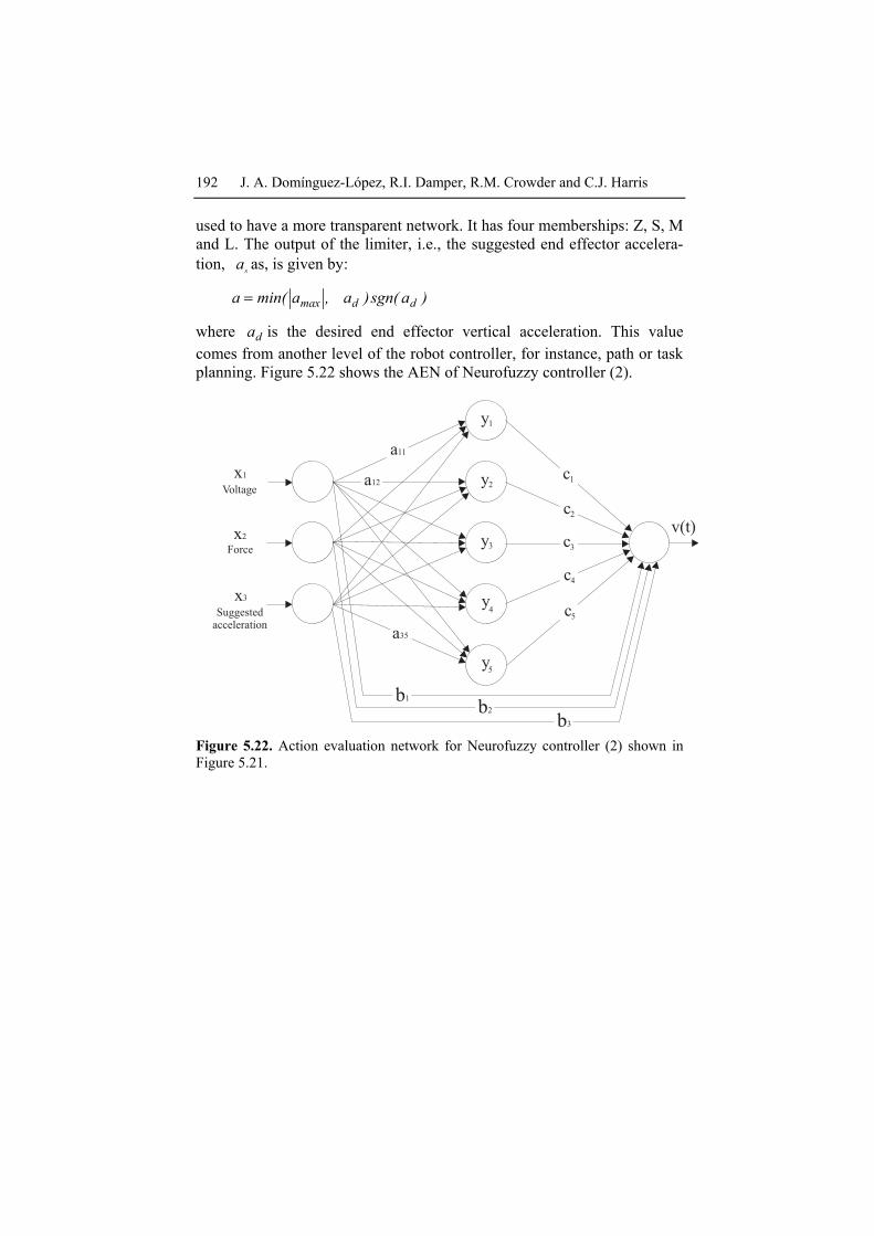
The output set of Neurofuzzy controller (2) is the maximum absolute acceleration ( )maxa . The absolute value of the maximum acceleration is
192 J. A. Domínguez-López, R.I. Damper, R.M. Crowder and C.J. Harris
used to have a more transparent network. It has four memberships: Z, S, M and L. The output of the limiter, i.e., the suggested end effector accelera-tion, sa as, is given by:
)asgn()a,amin(a ddmax= where da is the desired end effector vertical acceleration. This value comes from another level of the robot controller, for instance, path or task planning. Figure 5.22 shows the AEN of Neurofuzzy controller (2).
v(t)
1
x1
Suggestedacceleration
Force
Voltage
x2
x3
y
2y
3y
4y
5y
c1
c2
c3
c4
c5
a12
a11
a35
b1
b2
b3 Figure 5.22. Action evaluation network for Neurofuzzy controller (2) shown in Figure 5.21.
Applied motor voltage max-min
NVS Z VS S M L VL VVL
Z Z (1.0) Z (0.9) S (0.1)
Z (0.85) S (0.15)
Z (0.8) S (0.2
Z (0.7) S (0.3)
Z (0.6) S (0.4)
Z (0.6) S (0.4)
Z (0.7) S (0.3)
S L (0.9) M (0.1)
L (0.9) M (0.1)
L (0.85) M (0.15)
L (0.8) M (0.2)
L (0.8) M (0.2)
L (0.7) M (0.3)
L (0.5) M (0.5)
L (0.4) M (0.6)
M L (0.6) M (0.4)
L (0.5) M (0.5)
L (0.4) M (0.5) S (0.1)
L (0.2) M (0.6) S (0.2)
L (0.1) M (0.6) S (0.3)
M (0.5) S (0.5)
M (0.1) S (0.8) Z (0.1)
S (0.6) Z (0.4)
Fingertip force
L Z (0.2) S (0.8)
Z (0.4) S (0.6)
Z (0.6) S (0.4)
Z (0.7) S (0.3)
Z (0.8) S (0.2)
Z (0.8) S (0.2)
Z (0.95) S (0.05)
Z (1.0)
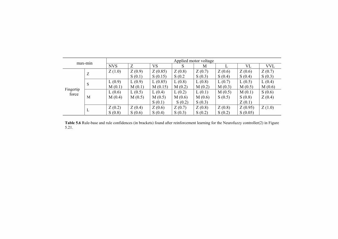
Table 5.6 Rule-base and rule confidences (in brackets) found after reinforcement learning for the Neurofuzzy controller(2) in Figure 5.21.

0 1 2 3 4 5 6 7 8 9 10−8
−6
−4
−2
0
2
4
6
8
Time (s)
Slip
rat
e (c
m/s
)
(a) Object slip
0 1 2 3 4 5 6 7 8 9 10−2
−1
0
1
2
3
4
Time (s)
App
lied
mot
or v
olta
ge (
V)
(b) End effector motor terminal voltage
0 1 2 3 4 5 6 7 8 9 100
500
1000
1500
2000
2500
3000
3500
Time (s)
App
lied
forc
e (m
N)
(c) Applied force
0 1 2 3 4 5 6 7 8 9 10−30
−20
−10
0
10
20
Time (s)
End
effe
ctor
ver
tical
acc
eler
atio
n (m
/s2 )
(d) Vertical acceleration: desired (dashed), suggested (solid)
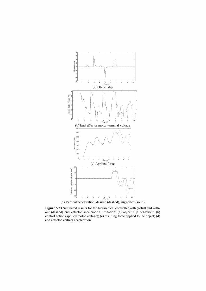
Figure 5.23 Simulated results for the hierarchical controller with (solid) and with-out (dashed) end effector acceleration limitation: (a) object slip behaviour; (b) control action (applied motor voltage); (c) resulting force applied to the object; (d) end effector vertical acceleration.
196 J. A. Domínguez-López, R.I. Damper, R.M. Crowder and C.J. Harris
Both neurofuzzy controllers share the same Markov decision process.
Neurofuzzy controller (1) is trained first; once its training has been com-pleted, Neurofuzzy controller (2) is trained. If the two neurofuzzy control-lers were trained simultaneously, it would be impossible to determine which controller was responsible for either failure or success. Table 5.6 shows the Neurofuzzy controller (2) rule base and rule confidences found after 45 minutes of reinforcement learning. The rule base of Neurofuzzy controller (1) corresponds to that of the neurofuzzy hierarchical controller (Tables 5.4 and 5.5). Figure 5.23 shows typical performance with and without acceleration limitation, subjected to the the standard pattern of dis-turbances. As illustrated by the dashed line in Figure 5.23(a), the hierar-chical end effector controller was able to eliminate the object slippage due to end effector vertical acceleration.
5.7 Conclusions
Robotic grippers are commonly used to restrain and manipulate a variety of objects under a wide range of conditions. Accordingly, robotic end ef-fectors are required to be capable of considerable gripping dexterity within an unstructured environment. The variety of objects and working condi-tions that might be met in practice make it impossible to foresee all the situations the system might encounter. Therefore, robotic systems need to be capable of dynamic adaptation to external disturbances, changing cir-cumstances and unforeseen situations. Ideally, the system should learn its adaptive behaviour on-line, through interaction with its environment, without the supervision of a ‘teacher’. This becomes vital when labelled training data are not available. However, when such training data are available, they can profitably be used to provide seed weights for on-line learning. Reinforcement learning is an effective way to train the neuro-fuzzy system on-line, facilitating adaptation to unexpected conditions. Its use led to successful control in situations where the supervised learning system failed.
Looking to have a faster adaptation to environmental changes, we have implemented a hybrid learning approach which uses both supervised and reinforcement learning. The combination of these two training algorithms allows the system to make good use of effective control actions discovered during operation. These can be considered as ‘labelled’ data since a record of inputs and outputs is continually kept over a preceding (three-second) period. The supervised learning scheme ran ‘in the background’ and was
5 Intelligent Neurofuzzy Control of a Robotic Gripper 197
only allowed to overwrite the results of reinforcement learning if the corre-sponding neurofuzzy network weights were not too dissimilar. In this way, the hybrid system can ‘ignore’ inconsistent (labelled) data. In addition, stability can be maintained (although not guaranteed) in the absence of a precise mathematical model of the system. The performance of the hybrid system was surprisingly good, recovering from simulated sensor failure much faster than the ‘pure’ reinforcement learning system.
In practice, all robot applications require end effector movement, so there will be end effector acceleration, which can induce slippage. Conse-quently, it is vital to validate the gripper controller under that condition. A controller without any information of the end effector acceleration treats this disturbance as any other (i.e., external force acting on the object). Al-though this controller is able to respond adequately over short time peri-ods, the continuous presence of acceleration could lead to the object slip-ping from the gripper. We therefore developed an approach using end effector acceleration feedback, integrating this extra input in the same fuzzy machine. This controller is indeed able to discover that in the exis-tence of acceleration, it has to apply more force. Thus, slippage is reduced. However, this improvement is at the cost of increasing the rule base, so re-ducing network transparency. At this point, the dilemma between model simplicity and model accuracy is evident. Hence, a parsimonious neuro-fuzzy hierarchical controller was proposed. With this approach, the num-ber of rules was smaller than required by the traditional neurofuzzy con-troller with acceleration feedback. The parsimonious controller had an excellent performance, allowing only slight slippage.
As with any large external force acting on the object, high accelerations of the effector will lead to slippage of the grasped object. The control technique proposed to solve this problem is again hierarchical. The addi-tion of a controller in charge of limiting the end effector acceleration im-proved noticeably the overall performance. However, such limitation strategies may have other unintended effects on the general performance of the robot. For instance, if the robot is path following, imposing a limit on acceleration places restrictions on the robot capabilities.
In conclusion, it is apparent that when the system has knowledge of a disturbance (i.e., acceleration), it is able to take a better action than when it is ignorant of such a disturbance. In the same way, when the system is able to modify the disturbance, it can help the controller to perform properly. Finally, the curse of dimensionality affects not only the system transpar-ency but also its learning speed and effectiveness. If the number of inputs increases, the system complexity increases too. A more complex system means that there are more possible neurons, weights and rules. Conse-
198 J. A. Domínguez-López, R.I. Damper, R.M. Crowder and C.J. Harris
quently, the learning problem is made harder. These drawbacks can be re-duced using parsimonious adaptive/product models.
References
1. Bicchi, A., V. Kumar, and IEEE, Robotic Grasping and Contact: A Review, in International Conference on Robotics & Automation. 2000: San Fransico. p. 348-53.
2. Dubey, V.N., Sensing and Control Within a Robotic End Effector, in Depart-ment of Electrical Engineering. 1997, University of Southampton: Southamp-ton, UK.
3. Chappell, P.H., M.M. Fateh, and R.M. Crowder, Kinematic Control of a Three-Fingered and Fully Adaptive End-Effector Using a Jacobian Matrix. Mechatronics, 2001. 11( 3): p. 355-368.
4. Dollar, A. and R. Howe, Towards Grasping in Unstructured environments: Optimization of Frasper Compliance and Configuration, in IEEE/RSJ Interna-tional Conference on Intelligent Robots and Systems. 2003: Las Vegas, Navada. p. 3410-6.
5. Nefti, S., et al., Intelligent Adaptive Mobile Robot Navigation. Journal of In-telligent and Robotic Systems, 2001. 30( 4): p. 311-329.
6. Brown, M. and C.J. Harris, Neurofuzzy Adaptive Modelling and Control. 1994, Hemel Hempstead, UK: Prentice Hall.
7. Kecman, V., Learning and Soft Computing. 2001, Cambridge, MA: MIT Press/Bradford Books.
8. Harris, C.J., X. Hong, and Q. Gan, Adaptive Modelling, Estimation and Fu-sion from Data: A Neurofuzzy Approach. 2002, Berlin and Heidelberg, Ger-many: Springer-Verlag.
9. Crowder, R.M., Sensors: Touch, Force, and Torque, in Handbook of Industrial Automation, R.L. Shell and E.L. Hall, Editors. 2000, Marcel Dekker: New York, NY. p. 377-392.
10. Domínguez-López, J.A., Intelligent Neurofuzzy Control in Robotic Manipula-tors, PhD in School of Electronics and Computer Science. May 2004, Univer-sity of Southampton: Southampton.
11. Brown, M. and C. Harris, Neurofuzzy Adaptive Modelling and Control. 1994, Hertfordshire, UK: Prentice Hall International.
12. Kecman, V., Learning and Soft Computing: Support Vector Machines, Neural Networks, and Fuzzy Logic Models. 2001, Boston, MA: MIT Press.
13. Jantzen, J., Neurofuzzy Modelling. 1998, Department of Automation, Techni-cal University of Denmark,: Lyngby, Denmark.
14. Driankov, D., H. Hellendoorn, and M. Reinfrank, An Introduction to Fuzzy Control. 1993, London, UK: Springer-Verlag.
15. Haykin, S., Neural Networks A Comprehensive Foundation. 1999, Upper Saddle River, NJ: Prentice-Hall.
5 Intelligent Neurofuzzy Control of a Robotic Gripper 199
16. Domínguez-López, J.A., et al. Hybrid neurofuzzy online learning for optimal grasping. in Proceedings of IEEE International Conference on Machine Learning and Cybernetics. 2003. Xi'an, China.
17. Kasabov, N., Evolving Fuzzy Neural Networks for Supervised/Unsupervised Online Knowledge-Based Learning. IEEE Transactions on Systems, Man, and Cybernetics, 2001. 31(6): p. 902-918.
18. Hertz, J., A. Krogh, and R.G. Palmer, Introduction to the Theory of Neural Computation. 1991, Reading, MA: Addison-Wesley.
19. Rumelhart, D.E., G.E. Hinton, and R.J. Williams, Learning representations by back-propagating errors. Nature, 1986. 323( 9): p. 533-536.
20. Chen, O.T.-C. and B.J. Sheu, Optimization Schemes for Neural Network Training, in IEEE International Conference on Neural Networks. 1994: Or-lando, FL. p. 817-822.
21. Sutton, R.S. and A.G. Barto, Reinforcement Learning: An Introduction. 2000, Cambridge, MA: MIT Press.
22. Sutton, R.S., Reinforcement learning architectures for animats, in From Ani-mals to Animats: Proceedings of the 1st International Conference on Simula-tion of Adaptive Behavior. 1991, Bradford Books/MIT Press: Cambridge, MA. p. 288-296.
23. Kaelbling, L.P., Foundations of learning in autonomous systems. Robotics and Autonomous Systems, 1991. 8: p. 131-144.
24. Watkins, C.J.C.H. and P. Dayan, Q-learning. Machine Learning, 1992. 8: p. 279-292.
25. Singh, S., P. Norving, and D. Cohn, A Tutorial Survey of Reinforcement Learning. Sadhana, 1994. 19( 6): p. 851-889.
26. Watkins, C.J.C.H., Automatic Learning of Efficient Behaviour, in Proceed-ings of First IEE International Conference on Artificial Neural Networks. 1989: London, UK. p. 395-398.
27. Sutton, R., S., A.G. Barto, and R.J. Williams, Reinforcement Learning is Di-rect Adaptive Optimal Control. IEEE Control Systems Magazine, 1992. 12( 2): p. 19-22.
28. Kaelbling, L.P., M.L. Littman, and A.W. Moore, Reinforcement Learning: A Survey. Journal of Artificial Intelligence Research, 1996. 4: p. 237-285.
29. Sutton, R.S., Learning to predict by the methods of temporal differences. Ma-chine Learning, 1988. 3( 1): p. 9-44.
30. Berenji, H. and P. Khedkar, Learning and Tuning Fuzzy Logic Controllers Through Reinforcements. IEEE Transactions on Neural Networks, 1992. 3( 5): p. 724-740.
31. Kolan, J. and J.B. Pollack, Back propergation is sensitive to initial conditions. Complex Systems, 1990. 4(3): p. 269-280.
32. Bellman, R., Adaptive Control Processes: A Guided Tour. 1961, Princeton, NJ: Princeton University Press.
33. Bishop, C.M., Neural Networks for Pattern Recognition. 1995, Oxford, UK: Oxford University Press.
200 J. A. Domínguez-López, R.I. Damper, R.M. Crowder and C.J. Harris
34. Bhanu, B., N. Thune, and M. Thune, CAOS: A Hierarchical Robot Control System, in Proceedings of the IEEE International Conference on Robotics and Automation. 1987: Raleigh, NC. p. 1603-1608.
35. Raju, G.V.S. and J. Zhou;, Adaptive Hierarchical Fuzzy Controller. IEEE Transactions on Systems, Man and Cybernetics, 1993. 23( 4): p. 973-980.
36. Mills, D.J., C.J. Harris, University of Southampton Technical Report, Neuro-fuzzy modelling and control of a six degree of freedom AUV. 1995.
37. Bossley, K.M., Neurofuzzy modelling approaches in system identification. 1997.
38. Brown, M. and C.J. Harris, A Perspective and Critique of Adaptive Neuro-fuzzy Systems used in Modelling and Control Applications. International Journal of Neural Systems, 1995. 6( 2): p. 197-220.