1

Neural Networks, Radial Basis Functions, and Complexity

Mark A. Kon1

Boston University and University of Warsaw

Leszek PlaskotaUniversity of Warsaw

1. Introduction

This paper is an introduction for the non-expert to the theory of artificial neuralnetworks as embodied in current versions of feedforward neural networks. There is a lot ofneural network theory which is not mentioned here, including the large body of work onnatural neural nets (i.e., the theory of neural networks in animals). For some excellentfoundational work on this topic, see [G1, G2]. We also include very recent work [KP]regarding what we consider to be the next important step in the theory of neural networksand their complexity, namely informational complexity theory for neural nets. In some sense this paper, being presented at a conference on condensed matter physics,follows a tradition which David Hestenes began at a conference on the maximum entropymethod in honor of Edward Jaynes, the father of this technique, which has been sosuccessful in the study and applications of condensed matter physics. In his contribution tothe proceedings of this conference [He], which we highly recommend, Hestenes presented apowerful argument for the viewpoint of Grossberg (see references above) in hisexplanations of numerous properties of natural neural networks in a set of equations knownas the which form a dynamical system with interesting properties inGrossberg equations, its own right, studied extensively by Hirsch and others. This however is as much as we willsay about work in the area of natural neural nets. For a general presentation of the theory ofartificial neural networks, including methods and approaches beyond the scope of thispaper, see [Ha]. The current emphasis on neural networks as a venue toward the eventual ideal ofartificial intelligent systems had its newest genesis in the mid-1980's, when it was realizedthat the classical von Neumann architecture (i.e., standard model of computation) was notcoming as close as some had hoped to true artificial intelligence, at the pace hoped for. Thevision of the 1960's, when the current field of artificial intelligence became popular, hadbeen that certainly by the year 2000, von Neumann architectures would be capable ofcoming close to simulating tasks which are called “intelligent.” At this point, around 1985-87, workers in many fields, including computer science, mathematics, physics, biology, andpsychology, began an interdisciplinary effort which continues to the present. A largeconference in San Diego with some 1500 participants in the “summer of networks” of 1987topped off a very rapid increase in interest in this area, which had previously beenmarginalized due to a variety of circumstances dating to the 1960's and earlier.

1Research partially supported by the National Science Foundation, Air Force Office of Scientific Research,and U.S. Fulbright Commission

2

The impetus for this “switch” of the hopes of many workers to neural nets came largelyfrom the “existence proof” which neural nets provide. Specifically, working neuralnetworks performing intelligent tasks certainly exist in the world today as natural neuralsystems. Applications of neural nets have been studied in physics, biology, psychology,engineering, and mathematics, and working artificial networks have been built to makedecisions on mortgage loan applications, identify properties of satellite photographs,balance a broom on its end, and a large number of other varied tasks. In this paper, we first introduce notions related to feedforward networks, including thoserelated to their most modern incarnations, so-called radial basis function (RBF) networks.We include a more detailed mathematical analysis of the approximation properties of suchRBF networks. Complexity issues for networks are covered in detail in the last severalsections, including very recent results of the authors in these areas. The reader willhopefully be convinced of the utility of the work in complexity (as well as see examples ofhow neural networks would work in a practical setting) in several examples given at theend.

2. Feedforward networks

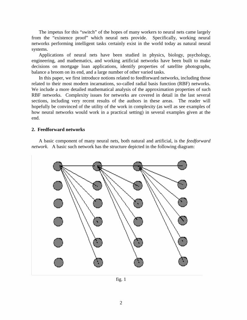
A basic component of many neural nets, both natural and artificial, is the feedforwardnetwork. A basic such network has the structure depicted in the following diagram:

fig. 1

3

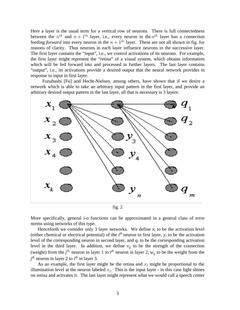
Here a layer is the usual term for a vertical row of neurons. There is full connectednessbetween the and layer, i.e., every neuron in the layer has a connection� � b � �!� !� !�

feeding into every neuron in the layer. These are not all shown in fig. forforward � b �!�

reasons of clarity. Thus neurons in each layer influence neurons in the successive layer.The first layer contains the “input”, i.e., we control activations of its neurons. For example,the first layer might represent the “retina” of a visual system, which obtains informationwhich will be fed forward into and processed in further layers. The last layer contains“output”, i.e., its activations provide a desired output that the neural network provides inresponse to input in first layer. Funahashi [Fu] and Hecht-Nielsen, among others, have shown that if we desire anetwork which is able to take an arbitrary input pattern in the first layer, and provide anarbitrary desired output pattern in the last layer, all that is necessary is 3 layers:

fig. 2

More specifically, general i-o functions can be approximated in a general class of errornorms using networks of this type. Henceforth we consider only 3 layer networks. We define to be the activation levelx i

(either chemical or electrical potential) of the neuron in first layer, to be the activationi yth i

level of the corresponding neuron in second layer, and to be the corresponding activation q i

level in the third layer. In addition, we define to be the strength of the connectionv ij

(weight) from the neuron in layer 1 to neuron in layer 2, to be the weight from thej i w !� th ij

j i th th neuron in layer 2 to in layer 3. As an example, the first layer might be the retina and might be proportional to the%�

illumination level at the neuron labeled This is the input layer - in this case light shines% i .

on retina and activates it. The last layer might represent what we would call a speech center

4

(neurons ultimately connected to a vocal device), and its pattern of neuron activationsqi

corresponds to verbal description about to be delivered of what is seen in first layer.

3. Neuron interaction rule

Neurons in one layer will be assumed to influence those in next layer in almost a linearway:

y = H v x - ,i

k

j=1ij j i : ;� �

i.e., activation is a linear function of activations in previous layer aside from the& Á� x j

modulating function ; here is a constant for each / �i i.

The function has on biological grounds traditionally been assumed a sigmoid:H

fig 3

Note that has a finite upper bound, so that response cannot exceed some fixed constant./

The activation in third layer has the form which is a linear function of the 's.q = w y , yi ij j j

n

j=1

� Our initial goal is to show here that we can get an arbitrary desired output pattern ofqi

activations on last layer as a function of inputs in the first layer. We can impose somexi

vector notation here -

x =

x

x

x {z }z }y |

1

2

k

%Å

will denote the vector of neuron activations in layer, while

5

V =

vv

v

i

i1

i2

ik

x {z }z }y |Å

denotes vector of connection weights from the neurons in first layer to the neuron in thei th

second layer. Now the activation of the second layer is:yi

y = H v x - = H V x - .i i

k

j=1

ij i: ;�

��� �² h ³

The activation in the third layer is q q = w y = W y.i i ij j

n

j=1

i� h

Thus we wish to show the activation pattern

q =

qq

q

x {z }z }y |

1

2

k Å

on the last layer (output) can be made an arbitrary function of the input activation pattern

x =

x

x

x {z }z }y |

1

2

k

%Å

À

Note the activation the of neuron in layer 3 is:ith

q = w y = w H V x - .i ij j ij j

n n

j=1 j=1

j� � ² h ³ ²� 3 1À ³

Thus our question is: if is defined by (3 1) (i.e., input determines output through a q = f x² ³ Àneural network equation), is it possible to approximate any function in this form? Speaking in the context of the above example, if the first layer represents the retina, thenif any input-output (i-o) function can be approximately encoded in the form 3 1 we can² À ³require that if represents the visual image of a chair (vector of pixel intensitiesx corresponding to chair), then represent the neural pattern of intensities corresponding to�articulation of the words “this is a chair.” Mathematically, we are asking, given any function , can we approximatef x² ³ ¢ ¦l lk k

f x² ³ with arbitrary precision by a function of the form (3 1) using various measures of�²%³ Àc

error, or norms (here represents -tuples of real numbers). What norms might we bel� �interested in? Some are:

6

P� c �P ~ O�²%³ c �²%³Oc c

P� c �P ~ �%O�²%³ c �²%³Oc c

P� c �P ~ �%O�²%³ c �²%³Oc c

*

%�

��

�

supl�

o��

or more generally, for any fixed , where� � �Á P� c �P ~ �%O�²%³ c �²%³Oc c

��

�°�8 9above sup denotes supremum. These norms are denoted as ( ) and finally theC L Llk Á Á�Á �

3 3 � P�P � BÀ� �� norms, respectively. In general denotes the class of functions such that

We say that a function approximates another function well in if is small. A� � 3 P� c �Pc c�

sequence converges to a function in if ¸� ¹ � 3 P� c �P �À� � ��~�

B � ­� ¦ B

It can be shown that the components of the above questions can be decoupled to theextent that they are equivalent to the case where there is only one Indeed, if any desiredq. i-o function can be approximated in systems with one output neuron, such single-outputsystems can be easily concatenated into larger ones (with more outputs) which haveessentially arbitrary approximable input-output properties. In any case, the configurationwe assume is therefore:

fig 4

7

Thus from (3.1):

q = w y = w H V x - .� �n n

j=1 j=1j j j j

j² h ³ ²� 3 2À ³

The fundamental question then is: Can any function be approximately f x : ² ³ lk ¦ l

represented exactly in this form? A partial answer has come in the form of the solution to Hilbert's 13th problem, whichwas constructed by Kolmogorov in 1957. He proved that continuous function f ¢ lk ¦ l

can be represented in the form

( ) ( ) f x = x .� �8 92k+1 k

j=1 i=1j ij i� �

where are continuous functions, and are monotone and independent of . That is, �j ij ij, f f� �

can be represented as sum of functions each of which depends just on a sum of singlevariable functions.

4. Some results on approximation

In 1987, Hecht-Nielsen showed that if we have 4 layers,

fig 5

then any continuous function can be approximated within in norm by such af x C² ³ �

network. The caveat here is that we do not yet have the techniques which will allow us toknow how many neurons it will take in the middle (so-called hidden) layers to accomplishthe job.

8

In 1989 Funahashi [Fu] proved:

Theorem: Let ( ) be a non-constant, bounded, and monotone increasing function. Let H x Kbe a compact (closed and bounded) subset of , and ( ) be a real-valued continuouslk f xfunction on :K

fig 6

Then for arbitrary > 0, there exist real constants and vectors such that� w , , j j� = �

f x = w H V x - ( ) ( ) 4.1)�n

j=1j j

j h ²�

satisfies

� � � ² Àf x - f x .( ) ( ) 4 2* � ³

This is the statement that functions of the form (4 1) are in the Banach space ( ) ofÀ dense C Kcontinuous functions on defined in the norm.2 � h �, *

Corollary: Functions of the form (4.1) are dense in for all . That is,L K p, 1 p < p² ³ � Bgiven any such , and an input-output function ( ) in ( ) i.e. such that < , andp f x L K , |f| dx p p B

� > 0, there exists an of the form (4.1) such that , i.e.,f f - f� � �p �

8 9�K

p|f - f | dx < �°�

�

9

The caveat of this Corollary, as indicated earlier is that we may need a very large hiddenlayer to accomplish this approximation within . An important practical question naturally�

is, how large will the hidden layer need to be to get such an approximation (e.g., how�

complex need a neural network be so that it is able to recognize a picture of a chair)? Someof these issues are touched in the brief discussion of complexity issues [KP] at the end ofthis paper.

5. Newer activation functions

Recall ( ) is assumed to be a sigmoid function having the form of fig. 3. The reasonH x for this choice is biological plausibility in natural networks. There are newer ideas whichhave been studied. For example, what is possible with a choice of a localized ( ): H x

fig 7

Such a choice, though not as biologically plausible, may work better. For example, couldHbe a wavelet Poggio, Girosi [GP] and others have pointed out that if ( ) cos on theÀ H x = xinterval [ , , we getc µ� �

f x = w V x - .( ) cos( ) 5.1�n

j=1j j

j h ²� ³

Now choose ( ) where are nonnegative integers, and = 0. ThenV = m = m ,m ,m , mj1 2 3 i jà �

f x = w cos m x .( ) ( )�

mm h

Now if

K = x ,x , ,x - x i x¸ à � � �( ) for = 2,3,... and 0 , 1 2 k i¢ � ¹� � 1 �

10

then this is just a multivariate Fourier cosine series in . Continuous functions can bexapproximated by multivariate Fourier series, and, as is well-known, we know how to findthe very easily:wj

w = f(x) m x dx,j�

²� ³h

� �� cos

where again denotes dimension. We can build the corresponding network immediately,�since we know what the weights need to be if we know the i-o function. This is a verypowerful concept as well as technique. Notice that ( ) here has the form H x

fig. 8

which is nothing like a sigmoid. Note there are questions of stability, however - if we makea small mistake in , then cos may vary wildly Nevertheless, in machine tasks thisx m xh Àmay not be as critical as in biological systems.

6. Radial basis functions

Recall that we have for the single neuron output system:

q = w y = w H V x - = f x� �n n

j=1 j=1j j j j

j( ) ( ).h �

We will now consider newer families of activation functions and neural network protocols.Instead of each neuron in hidden layer summing its inputs, in artificial systems there is noreason why it cannot take more complicated functions of inputs, for example a functionwhich is a bump defined on the variable % ~ ²% Áà Á % ³À� �

Assume now that is a fixed function in the form of a “bump” which is the/multidimensional analog of figure 7:

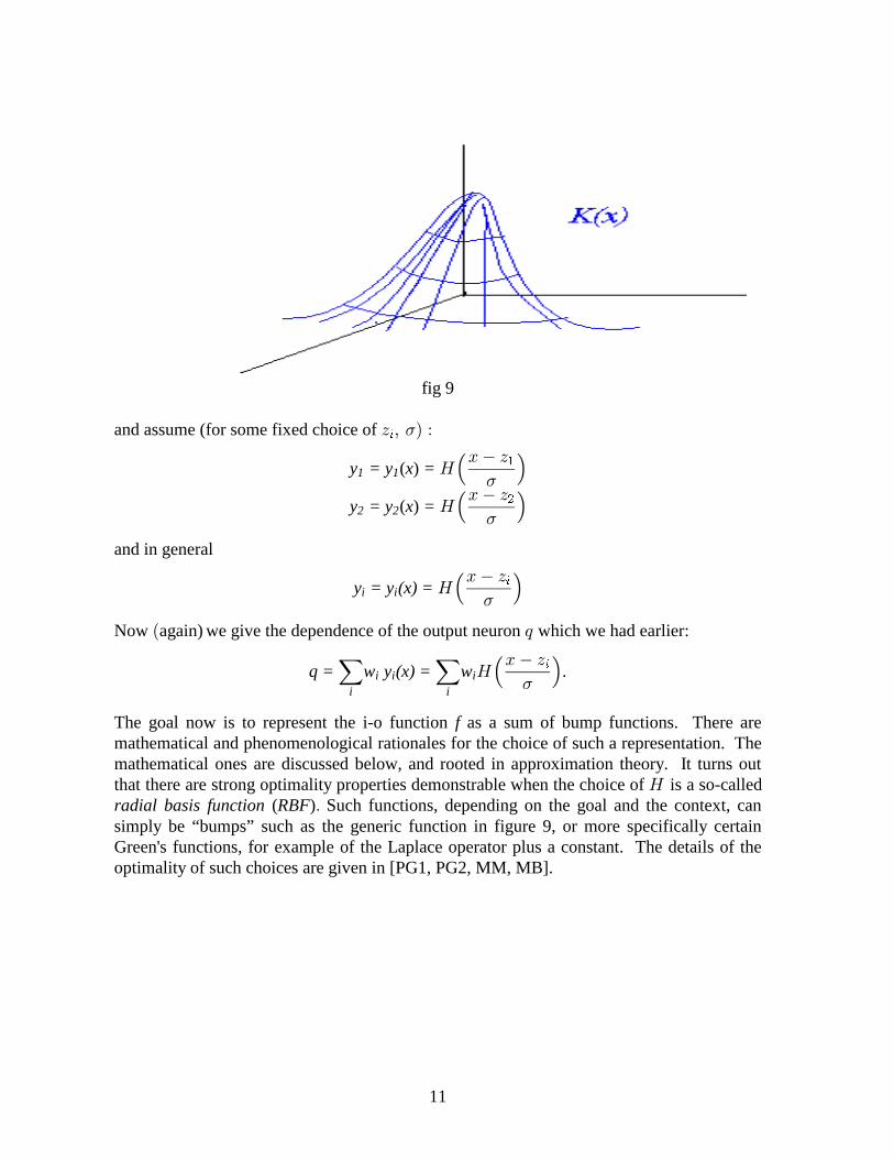
11

fig 9

and assume (for some fixed choice of ' Á ³ ¢� �

y = y x =

y = y x =

1 1

2 2

( )

( )

/

/

6 76 7% c '

% c '

�

�

�

�

and in general

y = y (x) = i i /6 7% c '��

Now again) we give the dependence of the output neuron which we had earlier:² �

q = w y (x) = w .� � 6 7

i ii i i/

%c '��

The goal now is to represent the i-o function as a sum of bump functions. There arefmathematical and phenomenological rationales for the choice of such a representation. Themathematical ones are discussed below, and rooted in approximation theory. It turns outthat there are strong optimality properties demonstrable when the choice of is a so-called/radial basis function RBF( ) Such functions, depending on the goal and the context, canÀsimply be “bumps” such as the generic function in figure 9, or more specifically certainGreen's functions, for example of the Laplace operator plus a constant. The details of theoptimality of such choices are given in [PG1, PG2, MM, MB].

12

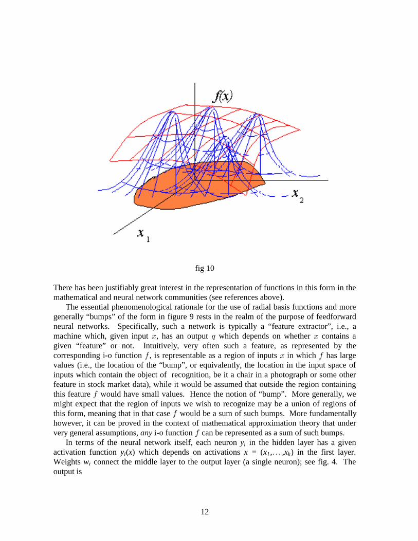
fig 10

There has been justifiably great interest in the representation of functions in this form in themathematical and neural network communities (see references above). The essential phenomenological rationale for the use of radial basis functions and moregenerally “bumps” of the form in figure 9 rests in the realm of the purpose of feedforwardneural networks. Specifically, such a network is typically a “feature extractor”, i.e., amachine which, given input , has an output which depends on whether contains a% � %given “feature” or not. Intuitively, very often such a feature, as represented by thecorresponding i-o function , is representable as a region of inputs in which has large� % �values (i.e., the location of the “bump”, or equivalently, the location in the input space ofinputs which contain the object of recognition, be it a chair in a photograph or some otherfeature in stock market data), while it would be assumed that outside the region containingthis feature would have small values. Hence the notion of “bump”. More generally, we�might expect that the region of inputs we wish to recognize may be a union of regions ofthis form, meaning that in that case would be a sum of such bumps. More fundamentally�however, it can be proved in the context of mathematical approximation theory that undervery general assumptions, i-o function can be represented as a sum of such bumps.any � In terms of the neural network itself, each neuron in the hidden layer has a givenyi

activation function ( ) which depends on activations ( ) in the first layer.y x x = x , ,xi 1 kÃWeights connect the middle layer to the output layer (a single neuron); see fig. 4. The w i

output is

13

q = w y x�n

i=1i i ( )

this should be a good approximation to the desired i-o function ( )q = f x . The best choice of weights is attained by choosing large if there is large “overlap”w wi i

between the desired i-o function ( ) and the given function ( ) (i.e., ( ) is f x y x = y xi i/4 5%c'�

�

large where ( ) is large):f x

fig 1�

Thus measures the “overlap” between ( ) and the activation function ( ).w f x y xi i

Usually there is one neuron which has the highest overlap ; in adaptive resonancey wi i

theory, this neuron is the “winner” and all other neurons are suppressed to have weight 0.Here however, each neuron provides a weight according to its “degree of matching” withwi

the desired ( ).f x Tomaso Poggio [Po], in his paper “A theory of how the brain might work” (1990) givesplausible arguments that something like this “matching" of desired i-o function againstbumps like ( ) may be at work in the brain (he discusses examples in facial recognitiony xi

and motor tasks in cerebellum).

7. Mathematical analysis of RBF networks: Mathematically, the class of functions we obtain from the above-described network hasthe form:

14

q x = w ,( ) 7 2� 6 7k

i=1i / ²

% c '��

À ³

where is a fixed function and are constants which may vary. The class of2 ¸zi Á�¹functions ( ) of this form will be called The question we will address, this time inq x S (K). 0

a mathematically more precise way, is, What functions ( ) can be approximated byf xf x( ) ?~ �²%³ Park and Sandberg [PS] answered this question (other versions of related questions haveappeared previously as well):

Theorem (Park and Sandberg (1993)): Assuming is integrable, is dense in ( ) if/ S L0r1 l

and only if 0/ £

Recall the definition (below (4.2)) of a dense collection of functions. In particular thecollection is dense in if for any function in and number there: 3 ² ³ � 3 ² ³ � ��

� � � �l l �

exists a in the class such that�²%³ :c

�

P� c �P ~ �%O�²%³ c �²%³O � Àc c

� � �

Thus any i-o function ( ) in (i.e., any integrable function) can be approximated to anf x L1

arbitrary degree of accuracy by a function of the form (7.2) in norm. We now provide aL1

sketch of the proof of the result of Park and Sandberg.

Sketch of Proof: CAssume that 0. Let denote continuous compactly supported/ £ c

(i.e., non-zero on a bounded set) functions on . Then any function in can beld L1

approximated arbitrarily well in norm by functions in , i.e., is dense in ; this is aL C C L1 1c c

standard fact of functional analysis. Thus to show that functions can be arbitrarily well approximated in norm byL L1 �

functions in it is sufficient to show that functions can be well approximated in byS , C L01

c

functions in i.e.` that for any function in there exists in such thatS , 0 � * � 3c

��

P� c �P �c

� � �. Choose > 0 and a function in such that1 C/c c

� / / � - < .c 1 1�

Let the constant Define , so that a = . (x) = a (x)�

/ �(x) dx c� /

� ��(x) dx = a (x) dx = /� 1.

Define A basic lemma we use here but do not prove is the fact that for� � �� �(x) = (x/ ). �

� h

�� in *�,

� �f - * f � � ��� ¦ Á 0

where denotes convolution.i

15

Thus functions of the form can be arbitrarily well approximated by * ; therefore itf f� ���is sufficient to show * can be approximated by functions in arbitrarily well. We now�� f S� 0

write (for below sufficiently large):;

( )( ) ( ) ( ) ( ) ( ) ( )� � � � � � � � �� � �* f = - x f x dx - f ,2Tn� �

´c;Á;µ

� � 8 9�

� #n i c i

n

i=1

r

�

r

where are all points of the form�i

[ ],-T + , -T + , , -T + 2i T 2i T 2i T

n n n1 2 r

Ã

so that we have one point in each sub-cube of size 2 . The convergence of RiemannT/nsums to their corresponding integrals implies that pointwise; then we can usev * fnn ¦SB �� �

the dominated convergence theorem of real analysis to show that convergence is also in L1ÀThus we can approximate by . Therefore we need to show that can be�� i �� v vn n

approximated by S .0

To this end, we have

v ( ) = n d

f 2T - n r r

n

0

c i ir

c�

� � �

� � � �

�

/ h/ � 8 9

r

( )( )( ) �

we then replace by (which we have shown can be made arbitrarily close), and we then/ /c

have something in completing the proof of the forward implication in the theorem.S 0

The converse of the theorem (only if part) is easy to show and is omitted here.

There is a second theorem for density in the norm. Define now toL S 21 ~ : ²/³�

consist of all functions of the form (( ) ) (the variable scale a x - z /�

ii i i/ � �� can depend on �

here).

We then have the following theorems, also in [PS]:

Theorem: Assuming that is square integrable, then ( ) is dense in ( ) if and only/ / S L1r2 l

if is non-zero on some set of positive measure./

Theorem: Assume that is integrable and continuous and (0) (i.e., the set of which/ / -1 %/ ¸ � ¹ $maps to 0) does not contain any set of the form 0 for any vector . Then ist : t S$ 1

dense in ( ) with respect to the sup norm for any compact set .C W W

This is an indication of what types of approximation results are possible in neuralnetwork theory. For a detailed analysis of approximation by neural nets, we refer the readerto [MM1-3; Mh1,2].

16

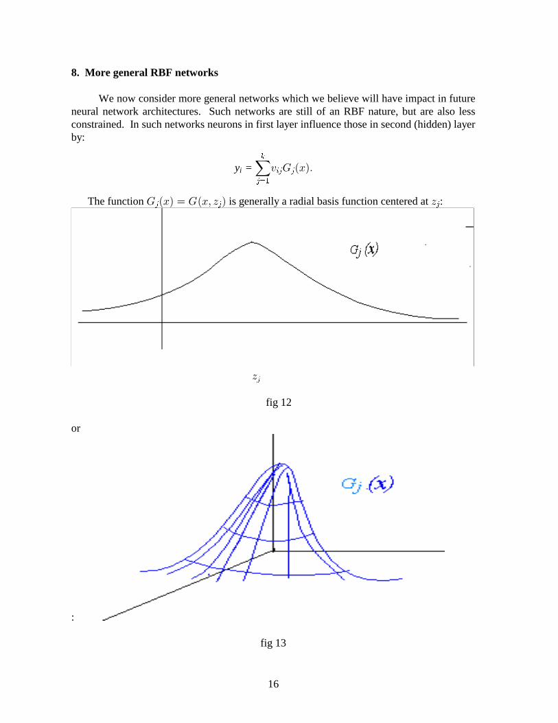
8. More general RBF networks

We now consider more general networks which we believe will have impact in futureneural network architectures. Such networks are still of an RBF nature, but are also lessconstrained. In such networks neurons in first layer influence those in second (hidden) layerby:

y = i � !�~�

�

�� �# . % 
The function is generally a radial basis function centered at : . ²%³ ~ .²%Á ' ³ '� � �

'�

fig 12

or

:

fig 13

17

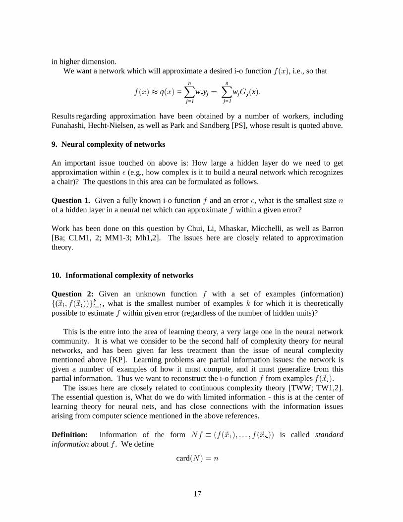
in higher dimension. We want a network which will approximate a desired i-o function , i.e., so that�²%³

�²%³ � ²%³ ~ . Àq = w y w x� � !n n

j=1 j=1j j� �

Results regarding approximation have been obtained by a number of workers, includingFunahashi, Hecht-Nielsen, as well as Park and Sandberg [PS], whose result is quoted above.

9. Neural complexity of networks

An important issue touched on above is: How large a hidden layer do we need to getapproximation within (e.g., how complex is it to build a neural network which recognizes�

a chair)? The questions in this area can be formulated as follows.

Question 1. Given a fully known i-o function and an error , what is the smallest size � ��

of a hidden layer in a neural net which can approximate within a given error?�

Work has been done on this question by Chui, Li, Mhaskar, Micchelli, as well as Barron[Ba; CLM1, 2; MM1-3; Mh1,2]. The issues here are closely related to approximationtheory.

10. Informational complexity of networks

Question 2: Given an unknown function with a set of examples (information)�¸ % Á �²% ³³¹ �W W( , what is the smallest number of examples for which it is theoretically� � �~�

�

possible to estimate within given error (regardless of the number of hidden units)?�

This is the entre into the area of learning theory, a very large one in the neural networkcommunity. It is what we consider to be the second half of complexity theory for neuralnetworks, and has been given far less treatment than the issue of neural complexitymentioned above [KP]. Learning problems are partial information issues: the network isgiven a number of examples of how it must compute, and it must generalize from thispartial information. Thus we want to reconstruct the i-o function from examples� �²% ³ÀW� The issues here are closely related to continuous complexity theory [TWW; TW1,2].The essential question is, What do we do with limited information - this is at the center oflearning theory for neural nets, and has close connections with the information issuesarising from computer science mentioned in the above references.

Definition: Information of the form is called 5� � ²�²% ³Áà Á �²% ³³W W� � standardinformation about . We define�

card²5³ ~ �

18

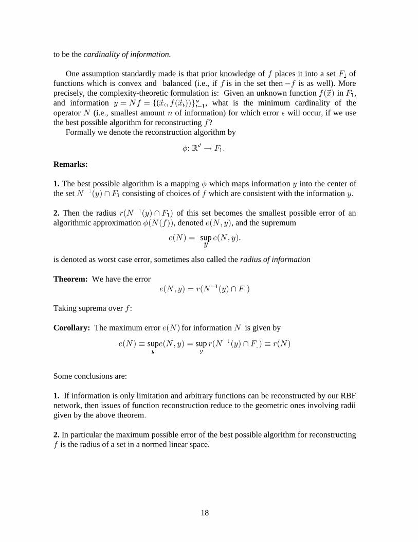
to be the cardinality of information. One assumption standardly made is that prior knowledge of places it into a set of� -�

functions which is convex and balanced (i.e., if is in the set then is as well). More� c�precisely, the complexity-theoretic formulation is: Given an unknown function in ,�²%³ -W �

and information {( , what is the minimum cardinality of the& ~ 5� ~ % Á �²% ³³¹W W� � �~�

�

operator (i.e., smallest amount of information) for which error will occur, if we use5 � �

the best possible algorithm for reconstructing ?� Formally we denote the reconstruction algorithm by

� l: ��¦ - À

Remarks:

1. The best possible algorithm is a mapping which maps information into the center of� &the set consisting of choices of which are consistent with the information 5 ²&³ q - � &Àc�

�

2. Then the radius of this set becomes the smallest possible error of an�²5 ²&³ q - ³c��

algorithmic approximation , denoted , and the supremum�²5²�³³ �²5Á &³

�²5³ ~ �²5Á &³&

sup .

is denoted as worst case error, sometimes also called the radius of information

Theorem: We have the error�²5Á &³ ~ �²5 ²&³ q - ³c�

�

Taking suprema over :�

Corollary: The maximum error for information is given by�²5³ 5

�²5³ � �²5Á &³ ~ �²5 ²&³ q - ³ � �²5³sup sup& &

c��

Some conclusions are:

1. If information is only limitation and arbitrary functions can be reconstructed by our RBFnetwork, then issues of function reconstruction reduce to the geometric ones involving radiigiven by the above theoremÀ

2. In particular the maximum possible error of the best possible algorithm for reconstructing� is the radius of a set in a normed linear space.

19

11. Informational and neural complexity

Definition: Define minimal error with information of cardinality to be� �²�³ �inf

card²5³~�

�²5³. Define the informational -complexity of function approximation in the set � -�

to be

�² ³ ~ ¸� ¢ �²�³ � ¹� �inf

Bounds on these quantities give informational complexities, i.e., how much information isneeded to bound within given error. These are geometric quantities related to notions�involving Gelfand radii of sets in a normed linear space. We now come to the general question involving the interaction of the two types ofcomplexities mentioned above.

Question 3. Question 1 Question 2 In we assume network size is the only limitation. In �we assume example number is only limitation. In practice both parameters are limited.�How do values of and interact in determining network error ?� � �

Here assume is a bounded set in a -� reproducing kernel Hilbert space (RKHS), i.e., -�

has an inner product defined for , along with a function such thatº� Á �» � Á � � - .²%Á &³�

for any ,� � -�

�²%³ ~ º.²%Á &³Á �²&³»

for all ; the inner product above is in This condition may sound formidable, but in� � - &À�

fact it is a minor restriction: if function values are defined and continuous operations,�²%³then is an RKHS.-�

We consider the interaction of the two complexity theories (neural and informational).Specifically, what is = number of neurons and = number of examples necessary to� �approximate within given error?� We wish to characterize interaction of the two complexities and , i.e., understand� �error as a function of both amount of information and available number of neurons. This isas yet not a well developed theory; see Poggio and Girosi [PG1,2]. The aims of this theory are:

• To develop algorithms which optimize information (i.e., number of examples) and numberof neurons necessary to compute i-o functions in given classes.�

• To show they apply to examples of interest in constructing RBF neural networks.

• To show radial basis function (RBF) algorithms are best-possible in very strong sense,and do define and describe theoretical and practical applications.

The conclusions of the theory in [KP] are:

20

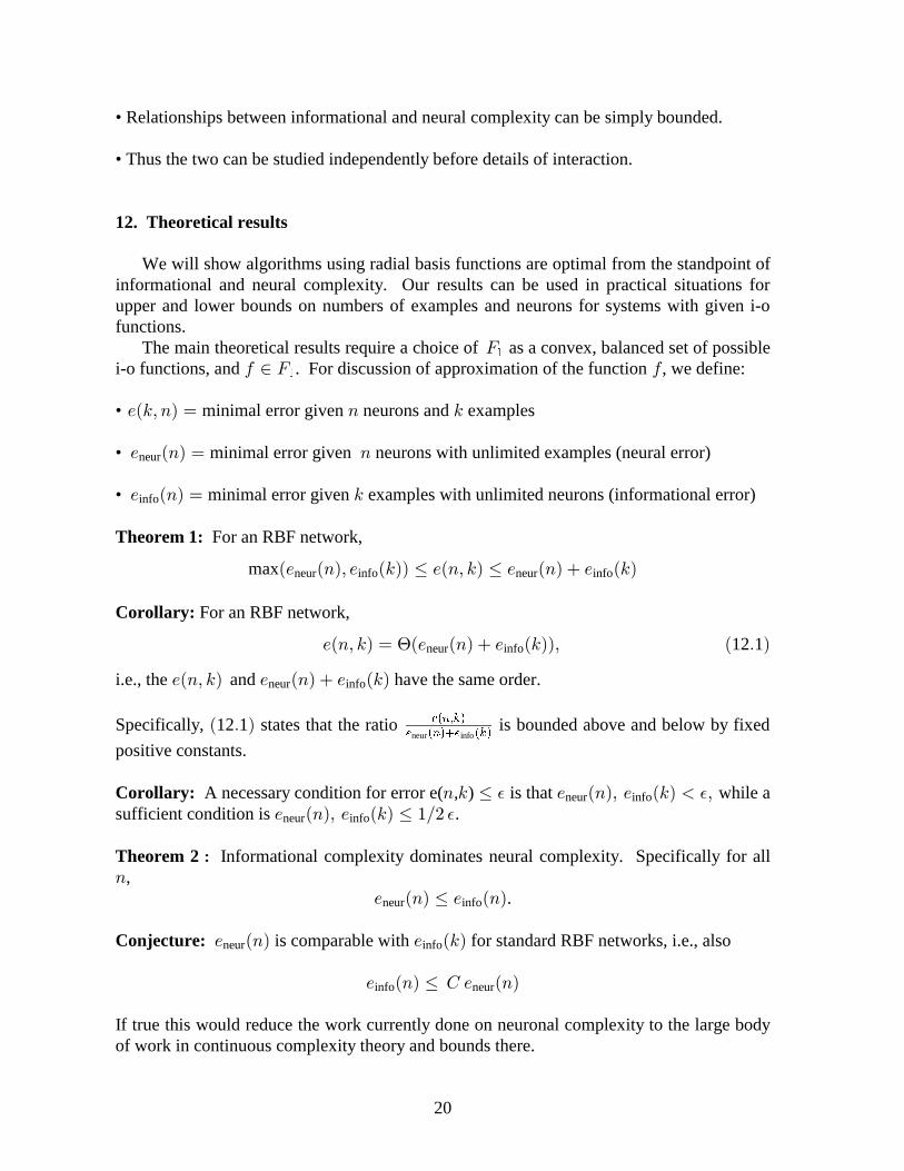
• Relationships between informational and neural complexity can be simply bounded.

• Thus the two can be studied independently before details of interaction.

12. Theoretical results

We will show algorithms using radial basis functions are optimal from the standpoint ofinformational and neural complexity. Our results can be used in practical situations forupper and lower bounds on numbers of examples and neurons for systems with given i-ofunctions. The main theoretical results require a choice of as a convex, balanced set of possible-�

i-o functions, and . For discussion of approximation of the function , we define:� � - ��

• minimal error given neurons and examples�²�Á �³ ~ � �

• minimal error given neurons with unlimited examples (neural error)� ²�³ ~ �neur

• minimal error given examples with unlimited neurons (informational error)� ²�³ ~ �info

Theorem 1: For an RBF network,

max²� ²�³Á � ²�³³ � �²�Á �³ � � ²�³ b � ²�³neur info neur info

Corollary: For an RBF network,

�²�Á �³ ~ ²� ²�³ b � ²�³³Á ² À ³# neur info 12 1

i.e., the and have the same order.�²�Á �³ � ²�³ b � ²�³neur info

Specifically, 12 1 states that the ratio is bounded above and below by fixed² À ³ �²�Á�³

� ²�³b� ²�³neur info

positive constants.

Corollary: A necessary condition for error e( , ) is that while a� � � � ²�³Á � ²�³ � Á� �neur info

sufficient condition is .� ²�³Á � ²�³ � �°�neur info �

Theorem 2 ¢ Informational complexity dominates neural complexity. Specifically for all�,

� ²�³ � � ²�³neur info .

Conjecture: � ²�³ � ²�³neur info is comparable with for standard RBF networks, i.e., also

� ²�³ � * � ²�³info neur

If true this would reduce the work currently done on neuronal complexity to the large bodyof work in continuous complexity theory and bounds there.

21

Theorem 3: If the number of neurons is larger than the number of examples, then� �(a) A strongly optimal algorithm for constructing the weights of the network$�

approximating is given by a linear combination , where is�²%³ ~ $ .²! Á h ³ .²!Á h ³s&W�

� ��

the family of radial basis functions and is the information vector,Á & & ~ �²% ³ÀW � �

(b) For information with bounded noise, is an optimal algorithm for the choice of fors &W ��

which optimizes regularization functional of the forms&W ~ � �

< �²�³ ~ P�P b O& c �²% ³O-

� �

�

� ��

Such algorithms have been studied by Poggio and Girosi [PG ].�Á �

Definition: An algorithm is one which is optimal up to a constant factor,almost optimal i.e., whose error is at most a constant factor times the optimal error.

Let be (� any almost optimal algorithm for finding neural network approximations withfull information.

Theorem 4:(a) The composite algorithm yields an approximation which is almost optimal in(� k s &W

the number of neurons and the number of examples.� �(b) If the above conjecture is true, then itself yields an almost optimal approximation.s &W

Classical (and more difficult) algorithms for programming neural networks includebackpropagation and the Boltzmann machine for neural nets.

13. Examples

A. Building a control system controlling homeostatic parameters of an industrial mixture:

Imagine an industrial system which can control the following input variables:

• Temperature• Humidity• Specific chemical contents• Other related parameters

Assume that the output variable in this case is the ratio of elasticity and strength of a plasticproduced from the above mixture. Combinations of input variables may have unpredictableeffects on output variable. Such effects include:

• binary correlations• tertiary correlations• more complicated interactions of inputs

22

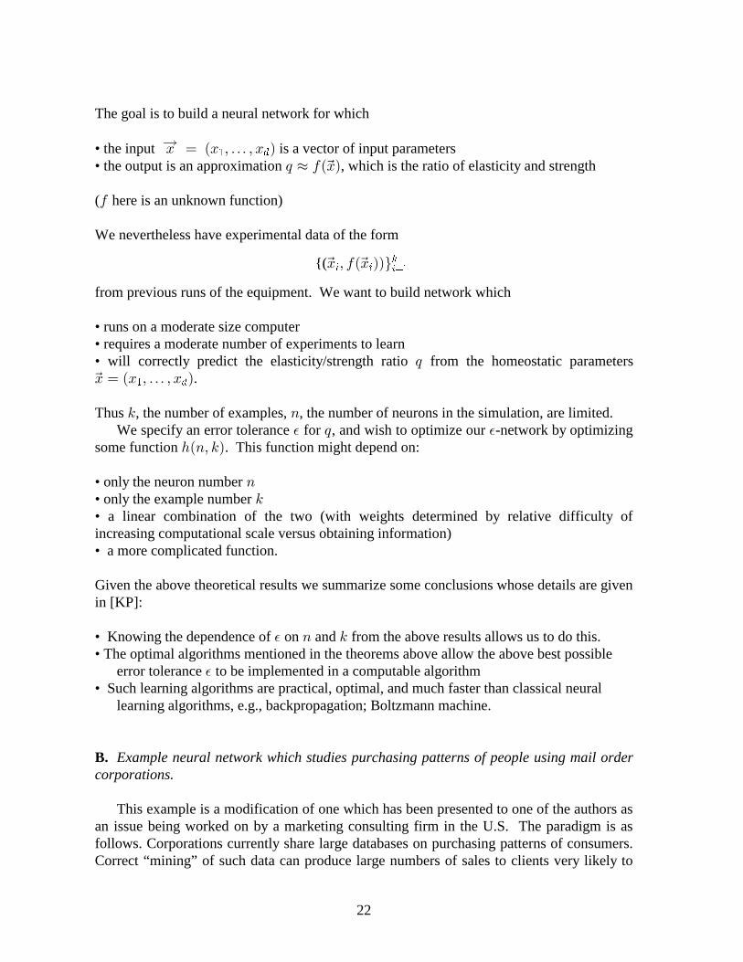
The goal is to build a neural network for which

• the input is a vector of input parameters% ~ ²% Áà Á % ³¦� �

• the output is an approximation , which is the ratio of elasticity and strength� � �²%³W

( here is an unknown function)�

We nevertheless have experimental data of the form

{( % Á �²% ³³¹W W� � �~�

�

from previous runs of the equipment. We want to build network which

• runs on a moderate size computer• requires a moderate number of experiments to learn• will correctly predict the elasticity/strength ratio from the homeostatic parameters�% ~W ²% Áà Á % ³� � .

Thus , the number of examples, , the number of neurons in the simulation, are limited.� � We specify an error tolerance for , and wish to optimize our -network by optimizing� ��some function . This function might depend on:�²�Á �³

• only the neuron number �• only the example number �• a linear combination of the two (with weights determined by relative difficulty ofincreasing computational scale versus obtaining information)• a more complicated function.

Given the above theoretical results we summarize some conclusions whose details are givenin [KP]:

• Knowing the dependence of on and from the above results allows us to do this.� � �• The optimal algorithms mentioned in the theorems above allow the above best possible error tolerance to be implemented in a computable algorithm�

• Such learning algorithms are practical, optimal, and much faster than classical neural learning algorithms, e.g., backpropagation; Boltzmann machine.

B. Example neural network which studies purchasing patterns of people using mail ordercorporations.

This example is a modification of one which has been presented to one of the authors asan issue being worked on by a marketing consulting firm in the U.S. The paradigm is asfollows. Corporations currently share large databases on purchasing patterns of consumers.Correct “mining” of such data can produce large numbers of sales to clients very likely to

23

purchase given product classes. A reasonable approach to predicting such patterns wouldbe as follows:

• create a tree structure on the family of products under consideration (e.g., one node would be appliances, a subnode would be kitchen appliances, and a sub- subnode ovens.),• input variables in the form of a vector for a given individual include% ~ ²% ÁÃ Á % ³W � �

dollar quantities of purchases .• The desired output is , the probability that the consumer will purchase a given target�²%³product, e.g., a blender, toaster, or oven.

The goal here is to find an algorithm yielding a network with the smallest practical error �

for our given information cardinality and computationally limited neuron cardinality .� �

Features of this particular scenario include:

• A large dimension of the input data (many products can be purchased),�• An unchangeable size of the learning set (� ¸ Á �² ³³¹% %W W� �

• The above results yield the minimal computational ability required to find a givenpurchase probability within given tolerance• The above algorithms can be used to find the best utilization of information andcomputational resources to compute .�² ³%W

14. Remarks on our assumptions:

We have here assumed that the i-o function belongs to a function class . A simple� -example of such an is , the set of functions with derivatives bounded by a- ) ²3 ³ �

B

constant If a function with small norm in the space can “well” approximate the�À � -i

unknown i-o function , it is unnecessary that be exactly smooth, or exactly belong to the� �indicated class. There must be a global fit which is acceptable, and under such assumptionsthese theorems can be applied. As an example, in the above homeostatic system, assume we know that the variation ofthe output quality is such that can be approximated by a 10 times differentiable�²%³ �function (e.g., a polynomial) whose first 10 derivatives are smaller than 15 (in someappropriate scale). In the context of polynomial approximation, for example, this placesbounds on the coefficients of the polynomials. Such bounds in this case would be areasonable way to “guess” the nature of the unknown function. We remark that suchbounds would be a heuristic process, with techniques and guidelines. Most importantly, the guesses made through such a process can be validated a posterioriwith the data subsequently obtained. For example, that the gradient of the data is boundedby, e.g., 15 units, can be verified experimentally; higher derivatives can be boundedsimilarly. The results of such an analysis might have the following features in a concrete situation:

24

• The I-O function can be well-approximated by a function in the Sobolev space , in� 3B

��

the ball of radius 15. This would provide our set and function space .- -�

• With this plus a given error tolerance, say .1, we can compute upper and lower� ~bounds for the informational and neural complexity of our problem using the above results.• We can then use the related RBF algorithm (mentioned in Theorem 3 above).• For example, such a calculation might show we need 10,000 examples and a networkwith 10,000 neurons (typically optimality is achieved with equal numbers by the aboveresults).

We mention a caveat here: we still will need to decide what examples to use; continuouscomplexity theory yields techniques only for choosing good data points as examples.

References

[Ba] A.R. Barron, Universal approximation bounds for superposition of a sigmoidal function, preprint, Yale University.[CLM1] C.K. Chui, X. Li, and H.N. Mhaskar, Neural networks for localized approximation, Center for Approximation Theory Report 289, 1993.[CLM2] C.K. Chui, Xin Li, and H. N. Mhaskar, Limitations of the approximation capabilities of neural networks with one hidden layer, Advances in Computational Mathematics (1996), 233-243.5[CL] C. K. Chui and X. Li, Approximation by ridge functions and neural networks with one hidden layer, (1992), 131-141.J. Approximation Theory 70[Fu] K. Funahashi. On the approximate realization of continuous mappings by neural networks, 183-192, 1989.Neural Networks2, [G1] Stephen Grossberg, Reidel Publishing Co., Boston, 1982Studies of Mind and Brain,[G2] Stephen Grossberg, North-Holland, Amsterdam, 1987The Adaptive Brain, [Ha] Mohamad Hassoun, , M.I.T. Press,Fundamentals of Artificial Neural Networks Cambridge, MA., 1995[He] D. Hestenes, How the Brain Works: the next great scientific revolution. In C.R. Smith and G.J. Erickson (eds.), Maximum Entropy and Bayesian Spectral Analysis and Estimation Problems, Reidel, Dordrecht/Boston (1987),173-205.[KP] M. Kon and L. Plaskota, Informational Complexity of Neural Networks, preprint.[MM1] H.N. Mhaskar and C.A. Micchelli, Approximation by superposition of sigmoidal and radial basis functions, (1992), 350-373.Advances in Applied Mathematics 13 [MM2] H.N. Mhaskar and C.A. Micchelli, Dimension independent bounds on the degree of approximation by neural networks, (1994), 277-IBM J. Research and Development38 284.[MM3] H. Mhaskar and C. Micchelli. Degree of approximation by neural and translation networks with a single hidden layer (1995) 151-Advances in Applied Mathematics161 , 183.[Mh1] H.N. Mhaskar., Neural networks for optimal approximation of smooth and analytic functions, (1996), 164-177.Neural Computation 8[Mh2] H.N. Mhaskar, Neural Networks and Approximation Theory, Neural Networks 9

25

(1996), 721-722.[MB] Micchelli, C.A. and M. Buhmann, On radial basis approximation on periodic grids, Math. Proc. Camb. Phil. Soc. 112 (1992), 317-334.[PS] Park, J. and I. Sandberg, Approximation and radial-basis-function networks, Neural Computation 5 (1993), 305-316.[PG1] T. Poggio, and F. Girosi, Regularization algorithms for learning that are equivalent to multilayer networks, (1990), 978-982.Science247[PG2] T. Poggio and F. Girosi, A theory of networks for approximation and learning, A.I. Memo No. 1140, M.I.T. A.I. Lab, 1989.[Po] T. Poggio. A theory of how the brain might work, In Proc. Cold Spring Harbor meeting on Quantitative Biology and the Brain, 1990.´TWW] Traub, J., G. Wasilkowski, and H. Wozniakowski, ,´ Information-Based Complexity Academic Press, Boston, 1988.´TW1] Traub, Joseph and Henryk Wozniakowski, ,´ A General Theory of Optimal Algorithms Academic Press, New York, 1980.´TW2] Joseph Traub and Henryk Wozniakowski, Breaking intractability, ´ Scientific American 270 (Jan. 1994), 102-107.

26

[MB] Micchelli, C.A. and M. Buhmann, On radial basis approximation on periodic grids, Math. Proc. Camb. Phil. Soc. 112 (1992), 317-334.[PS] Park, J. and I. Sandberg, Approximation and radial-basis-function networks, Neural Computation 5 (1993), 305-316.[PG1] T. Poggio, and F. Girosi, Regularization algorithms for learning that are equivalent to multilayer networks, (1990), 978-982.Science247[PG2] T. Poggio and F. Girosi, A theory of networks for approximation and learning, A.I. Memo No. 1140, M.I.T. A.I. Lab, 1989.[Po] T. Poggio. A theory of how the brain might work, In Proc. Cold Spring Harbor meeting on Quantitative Biology and the Brain, 1990.´TWW] Traub, J., G. Wasilkowski, and H. Wozniakowski, ,´ Information-Based Complexity Academic Press, Boston, 1988.´TW1] Traub, Joseph and Henryk Wozniakowski, ,´ A General Theory of Optimal Algorithms Academic Press, New York, 1980.´TW2] Joseph Traub and Henryk Wozniakowski, Breaking intractability, ´ Scientific American 270 (Jan. 1994), 102-107.