Application of the radial basis function neural network to ... · Application of the RBFN CREWES Research Report Š Volume 14 (2002) 1 Application of the radial basis function neural

Application of the RBFN

CREWES Research Report � Volume 14 (2002) 1

Application of the radial basis function neural network to the prediction of log properties from seismic attributes

Brian H. Russell, Laurence R. Lines, and Daniel P. Hampson1

ABSTRACT In this paper, we use the radial basis function neural network, or RBFN, to predict

reservoir log properties from seismic attributes. We also compare the results of this approach with the use of the generalized regression neural network, GRNN, for the same problem, as proposed by Hampson et al (2001). We discuss both the theory behind these methods and the methodology involved in applying neural networks to seismic attributes. We then illustrate the method using the Blackfoot 3D seismic volume, a channel sand example from Alberta.

INTRODUCTION

The prediction of reservoir parameters from seismic data has traditionally been done using deterministic methods, in which we assume a mathematical model that relates our observed seismic data to the reservoir parameter of interest, and apply an inverse transform to our seismic data based on this model. Such methods include deconvolution, post-stack trace inversion, and linearized pre-stack trace inversion, or AVO. These methods are limited by a number of factors, including noise in the seismic data, incorrect scaling of the seismic data, and limiting assumptions in the model (for example, we often ignore the fact the seismic wavelet is time-varying). There is also a fundamental ambiguity in the derivation of the long period component of the earth properties if we use the seismic data alone. To try to avoid the last problem, we may use inversion methods which are model-based, in that they use an initial model of the earth computed from more detailed well log measurements, and then perturb this model to fit the seismic observations.

In more recent approaches, a statistical, rather than deterministic, method is used to

look for a relationship between the seismic data and the reservoir parameters. These methods are based on traditional multi-regression, or on neural networks. For example, Ronen et al. (1994) proposed the use of the radial basis function neural network (RBFN) for the seismic-guided estimation of log properties. They applied the RBFN to averaged intervals from log data and the corresponding averaged intervals from the 3D seismic data volumes which were tied by these logs. In more recent work (Hampson et al, 2001), neural networks were used to predict reservoir log properties from the complete 3D seismic volume, using each log sample over the zone of interest in the training phase. In this latter approach, the generalized regression neural network, or GRNN, was used for the prediction of log properties, although this method was referred to in this paper as the probabilistic neural network, or PNN. (As we will see in the following theory section the PNN approach is a classification technique which is the basis upon which the GRNN method is built). In this paper, we extend the RBFN method to the computation of log properties from the full 3D seismic volume, and show the relationship between the RBFN and GRNN methods. Although both methods are based on the application of Gaussian 1 Hampson-Russell Software Services Ltd, 510, 715 � 5th Avenue SW, Calgary, Alberta, T2P 2X6

Russell, Lines, and Hirsche

2 CREWES Research Report � Volume 14 (2002)

weighting functions to distances measured in multiple seismic attribute space, they are quite distinct in their calculation of the final result.

Following a discussion of the theory behind the neural network techniques used here,

we will discuss the methodology for applying the methods to seismic data and then illustrate the methods with a channel sand case study from Alberta.

INTRODUCTION TO NEURAL NETWORKS

First of all, what is a neural network? The simplest answer is that a neural network is a mathematical algorithm that can be trained to solve a problem that would normally require human intervention. Although there are many different types of neural networks, there are two ways in which they are categorized: by the type of problem that they can solve and by their type of learning.

Neural network applications in seismic data analysis generally fall into one of two

categories: the classification problem, or the prediction problem. In the classification problem, we assign an input sample to one of several output classes, such as sand, shale, limestone etc, whereas in the prediction problem we assign a specific value to the output sample, such as a porosity value. A companion paper in this volume (Russell et al, 2002) discusses the application of two different neural networks, the multi-layer perceptron (MLP) and the radial basis function neural network (RBFN) to a straightforward AVO classification problem. In this paper, we will be concerned with the prediction problem, specifically the prediction of P-wave velocity from seismic attributes.

Neural networks can also be classified by the way they are trained, using either

supervised or unsupervised learning. In supervised learning the neural network starts with a training dataset for which we know both the input and output values. The neural network algorithm then �learns� the relationship between the input and output from this training dataset, and finally applies the �learned� relationship to a larger dataset for which we do not know the output values. Examples of the supervised learning approach are the MLP, the PNN, the GRNN, and the RBFN, of which the latter three methods will be used today. In unsupervised learning, we present the neural network with a series of inputs and let the neural network look for patterns itself. That is, the specific outputs are not required. The advantage of this approach is that we do not need to know the answer in advance. This disadvantage is that it is often difficult to interpret the output. An example of this type of unsupervised technique is the Kohonen Self Organizing Map (KSOM) (Kohonen, 2001).

THEORY

As mentioned in the last section, in this paper we will be using neural networks to

perform the supervised prediction of reservoir parameters. Our training dataset will consist of a set of N known training samples ti, which in our case will be some well log derived reservoir parameter such as VP, SP, SW, etc. Each training sample, which is a scalar quantity, is in turn dependant on a vector of L seismic attribute values, correlated in time with the training samples. (The issues of which seismic attributes to use and how to optimize the correlation between the training samples and the seismic data are



themselves difficult problems, and will be dealt with in the next section.) These seismic attribute vectors can be written si = (si1, si2, �, siL)T, i = 1, 2, �, N. The objective of our neural network is to find some function y such that:

y(si ) = ti , i =1, 2,�, N (1)

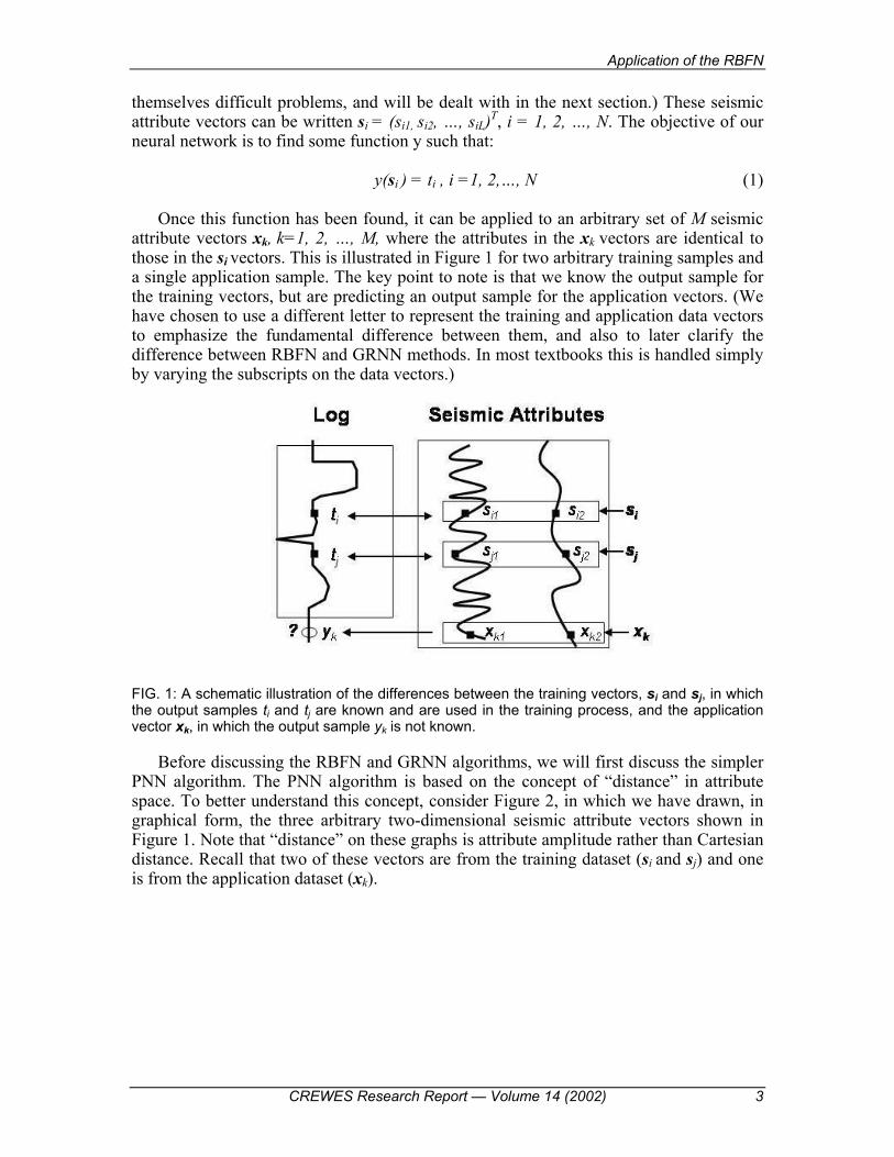
Once this function has been found, it can be applied to an arbitrary set of M seismic attribute vectors xk, k=1, 2, �, M, where the attributes in the xk vectors are identical to those in the si vectors. This is illustrated in Figure 1 for two arbitrary training samples and a single application sample. The key point to note is that we know the output sample for the training vectors, but are predicting an output sample for the application vectors. (We have chosen to use a different letter to represent the training and application data vectors to emphasize the fundamental difference between them, and also to later clarify the difference between RBFN and GRNN methods. In most textbooks this is handled simply by varying the subscripts on the data vectors.)

FIG. 1: A schematic illustration of the differences between the training vectors, si and sj, in which the output samples ti and tj are known and are used in the training process, and the application vector xk, in which the output sample yk is not known.

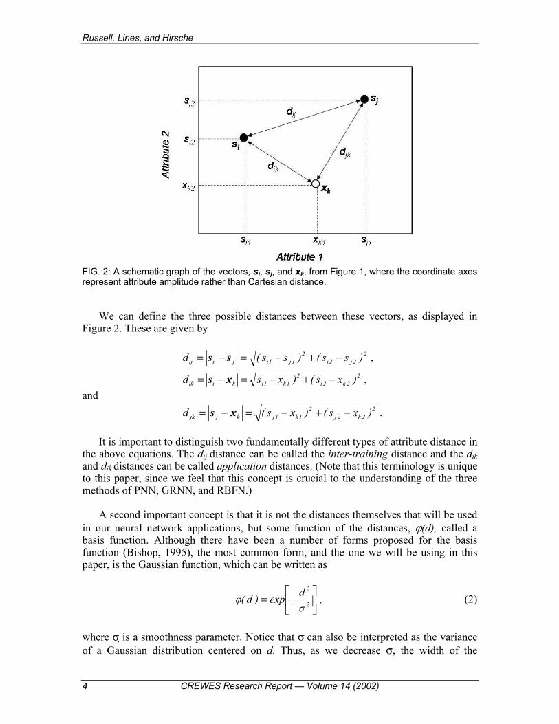
Before discussing the RBFN and GRNN algorithms, we will first discuss the simpler PNN algorithm. The PNN algorithm is based on the concept of �distance� in attribute space. To better understand this concept, consider Figure 2, in which we have drawn, in graphical form, the three arbitrary two-dimensional seismic attribute vectors shown in Figure 1. Note that �distance� on these graphs is attribute amplitude rather than Cartesian distance. Recall that two of these vectors are from the training dataset (si and sj) and one is from the application dataset (xk).



FIG. 2: A schematic graph of the vectors, si, sj, and xk, from Figure 1, where the coordinate axes represent attribute amplitude rather than Cartesian distance.

We can define the three possible distances between these vectors, as displayed in

Figure 2. These are given by 2

2j2i2

1j1ijiij )ss()ss(d −+−=−= ss ,

22k2i

21k1ikiik )xs()xsd −+−=−= xs ,

and 2

2k2j2

1k1jkjjk )xs()xs(d −+−=−= xs .

It is important to distinguish two fundamentally different types of attribute distance in the above equations. The dij distance can be called the inter-training distance and the dik and djk distances can be called application distances. (Note that this terminology is unique to this paper, since we feel that this concept is crucial to the understanding of the three methods of PNN, GRNN, and RBFN.)

A second important concept is that it is not the distances themselves that will be used

in our neural network applications, but some function of the distances, ϕ(d), called a basis function. Although there have been a number of forms proposed for the basis function (Bishop, 1995), the most common form, and the one we will be using in this paper, is the Gaussian function, which can be written as

−= 2

2

σdexp)d(φ , (2)

where σ is a smoothness parameter. Notice that σ can also be interpreted as the variance of a Gaussian distribution centered on d. Thus, as we decrease σ, the width of the



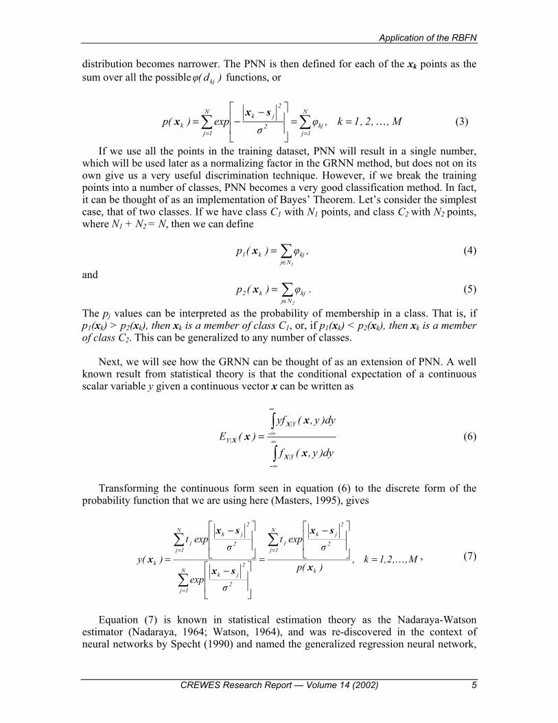
distribution becomes narrower. The PNN is then defined for each of the xk points as the sum over all the possible )d(φ kj functions, or

∑ ∑= =

==

−−=

N

1j

N

1jkj2

2

jkk M,,2,1k,φ

σexp)(p …

sxx (3)

If we use all the points in the training dataset, PNN will result in a single number, which will be used later as a normalizing factor in the GRNN method, but does not on its own give us a very useful discrimination technique. However, if we break the training points into a number of classes, PNN becomes a very good classification method. In fact, it can be thought of as an implementation of Bayes� Theorem. Let�s consider the simplest case, that of two classes. If we have class C1 with N1 points, and class C2 with N2 points, where N1 + N2 = N, then we can define

∑∈

=1Nj

kjk1 ,φ)(p x (4)

and ∑∈

=2Nj

kjk2 φ)(p x . (5)

The pj values can be interpreted as the probability of membership in a class. That is, if p1(xk) > p2(xk), then xk is a member of class C1, or, if p1(xk) < p2(xk), then xk is a member of class C2. This can be generalized to any number of classes.

Next, we will see how the GRNN can be thought of as an extension of PNN. A well known result from statistical theory is that the conditional expectation of a continuous scalar variable y given a continuous vector x can be written as

∫

∫∞

∞

∞

∞=

-X

-X

X

x

xx

dy)y,(f

dy)y,(yf)(E

Y|

Y|

|Y (6)

Transforming the continuous form seen in equation (6) to the discrete form of the

probability function that we are using here (Masters, 1995), gives

M,,2,1k,)(p

σexpt

σexp

σexpt

)(yk

N

1j2

2

jkj

N

1j2

2

jk

N

1j2

2

jkj

k …=

−

=

−

−

=

∑

∑

∑=

=

=

x

sx

sx

sx

x , (7)

Equation (7) is known in statistical estimation theory as the Nadaraya-Watson

estimator (Nadaraya, 1964; Watson, 1964), and was re-discovered in the context of neural networks by Specht (1990) and named the generalized regression neural network,



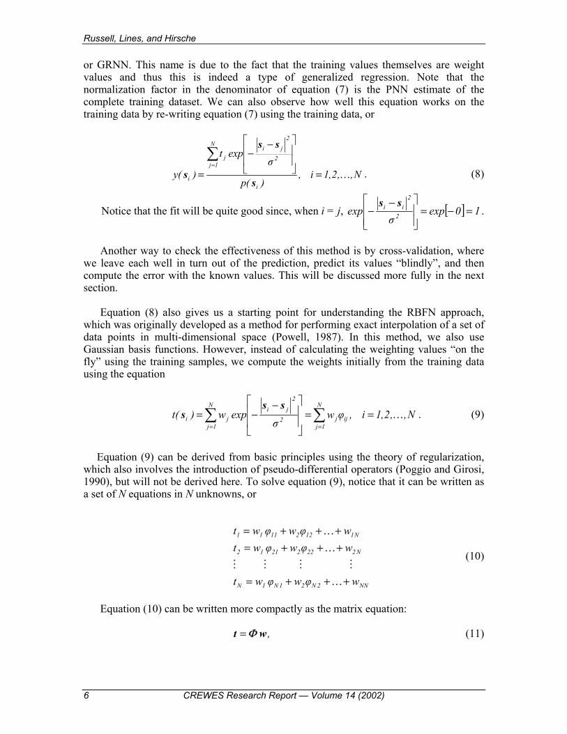
or GRNN. This name is due to the fact that the training values themselves are weight values and thus this is indeed a type of generalized regression. Note that the normalization factor in the denominator of equation (7) is the PNN estimate of the complete training dataset. We can also observe how well this equation works on the training data by re-writing equation (7) using the training data, or

N,,2,1i,)(p

σexpt

)(yi

N

1j2

2

jij

i …=

−−

=

∑=

s

ss

s . (8)

Notice that the fit will be quite good since, when i = j, [ ] 10expσ

exp 2

2ii =−=

−−

ss.

Another way to check the effectiveness of this method is by cross-validation, where

we leave each well in turn out of the prediction, predict its values �blindly�, and then compute the error with the known values. This will be discussed more fully in the next section.

Equation (8) also gives us a starting point for understanding the RBFN approach,

which was originally developed as a method for performing exact interpolation of a set of data points in multi-dimensional space (Powell, 1987). In this method, we also use Gaussian basis functions. However, instead of calculating the weighting values �on the fly� using the training samples, we compute the weights initially from the training data using the equation

N,,2,1i,φwσ

expw)(tN

1j

N

1jijj2

2

jiji …==

−−=∑ ∑

= =

sss . (9)

Equation (9) can be derived from basic principles using the theory of regularization,

which also involves the introduction of pseudo-differential operators (Poggio and Girosi, 1990), but will not be derived here. To solve equation (9), notice that it can be written as a set of N equations in N unknowns, or

NN2N21N1N

N22222112

N11221111

wφwφwt

wφwφwtwφwφwt

+++=

+++=+++=

…""""

……

(10)

Equation (10) can be written more compactly as the matrix equation:

,wt Φ= (11)



where

=

=

=

NN

N1

1N

11

N

1

N

1

φ

φ

φ

φand,

w

w,

t

t"

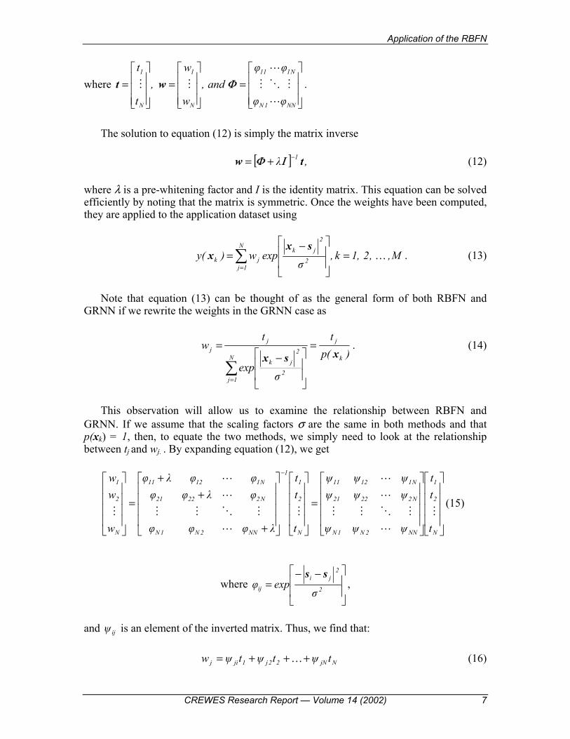
#$#""" Φwt .

The solution to equation (12) is simply the matrix inverse

[ ] ,λ 1 tw −+= ΙΦ (12)

where λ is a pre-whitening factor and I is the identity matrix. This equation can be solved efficiently by noting that the matrix is symmetric. Once the weights have been computed, they are applied to the application dataset using

M,,2,1k,σ

expw)(yN

1j2

2

jkjk …=

−=∑

=

sxx . (13)

Note that equation (13) can be thought of as the general form of both RBFN and

GRNN if we rewrite the weights in the GRNN case as

)(pt

σexp

tw

k

j

N

1j2

2

jk

jj xsx

=

−=

∑=

. (14)

This observation will allow us to examine the relationship between RBFN and

GRNN. If we assume that the scaling factors σ are the same in both methods and that p(xk) = 1, then, to equate the two methods, we simply need to look at the relationship between tj and wj. . By expanding equation (12), we get

=

+

++

=

−

N

2

1

NN2N1N

N22221

N11211

N

2

11

NN2N1N

N22221

N11211

N

2

1

t

tt

ψψψ

ψψψψψψ

t

tt

λφφφ

φλφφφφλφ

w

ww

"#

"$""##

"#

"$""##

"(15)

where

−−= 2

2ji

ij σexpφ

ss,

and ijψ is an element of the inverted matrix. Thus, we find that:

NjN22j1jij tψtψtψw +++= … (16)



In other words, wj is a weighted sum of all the training values. If the inverted matrix

consisted only of values along the main diagonal, we could rewrite the above equation as jjjj tψw = (17)

If this is the case,Φ would consist only of the values jjφ along the main diagonal.

But note that

1σ

expφ 2

2jj

jj =

−−=

ss

Thus, Φ = I, the identity matrix, and Φ−1 = I also. Therefore, for this trivial case, the RBFN and GRNN methods are identical to a scale factor. This would occur in two situations: (1) ,0ss ji ≈− for all i and j, and (2) 0→σ

In he more general case, the off-diagonal elements in the covariance matrix are all non-zero. Indeed, they will only be equal to zero for the case in which the seismic attributes are statistically independent. Thus, we can think of the GRNN method as a subset of the RBFN method for the case of statistical independence of the attributes. We would therefore expect the RBFN method to give a more high resolution result than the GRNN method, since the off-diagonal covariance elements are being used. As we shall see in our case study, this is indeed the case.

METHODOLOGY The methodology for reservoir prediction using multiple seismic attributes has been

extensively covered by Hampson et al (2001) and will only be briefly reviewed here. The two key problems in the analysis can be summarized as follows: which attributes should we use, and which of these attributes are statistically significant?

To start the process, we compute as many attributes as possible. These attributes can

be the classical instantaneous attributes of Taner et al. (1974), frequency and absorption attributes based on windowed estimates along the seismic trace, integrated seismic amplitudes, model-based trace inversion, or AVO intercept and gradient. Once these attributes have been computed and stored, we measure a goodness of fit between the attributes and the training samples from the logs. Using the notation of the previous section, we can compute this goodness of fit by minimizing the least-squares error given by

∑=

−−−−=N

1i

2LiLi110i

2 )swswwt(N1E … . (18)

Note that the weights can also be convolutional, as discussed by Hampson et al. (2001), which is equivalent to introducing a new set of time-shifted attributes. The attributes to use in the neural network computations, and their order is then found by a technique called stepwise regression, which consists of the following steps:



(1) Find the best attribute by an exhaustive search of all the attributes, using equation (1) to compute the prediction error for each attribute (i.e. L = 1) and choosing the attribute with the lowest error.

(2) Find the best pair of attributes from all combinations of the first attribute and one other. Again, the best pair is the pair that has the lowest prediction error from equation (18), with L = 2.

(3) Find the best triplet, using the pair from step (2) and combining them with each other attribute.

(4) Continue the process as long as desired. This will give us a set of attributes that is guaranteed to reduce the total error as the

number of attributes goes up. So, when do we stop? This is done using a technique called cross-validation, in which we leave out a training sample and then predict it from the other samples. We then re-compute the error using equation (18), but this time from the training sample that was left out. We repeat this procedure for all the training samples, and average the error, giving us a total validation error. This computation is done as a function of the number of attributes, and the resulting graph usually shows an increase in validation error past some small number of attributes such as five or six. In actual fact, we do not perform this procedure for all samples, but rather on a well by well basis. The next section will give an illustration of this procedure.

One final point to discuss is the optimization of the sigma values. The first point to

observe is that, in genera, the optimum sigma value for the GRNN method will be different than the optimum value for the RBFN method. A second important point is that, for the GRNN method, we also determine a different sigma value for each attribute. This could be introduced in equation (3) or (7) by changing the φkj term to

( ) ( ) ( )

−++

−+

−= 2

L

2jLkL

22

22j2k

21

21j1k

kj σsx

σsx

σsx

expφ … ,

where L is equal to the number of attributes. The optimization technique used for GRNN is described by Masters (1995).

A CHANNEL SAND CASE STUDY We will now illustrate our methodology using a channel sand case study from Alberta,

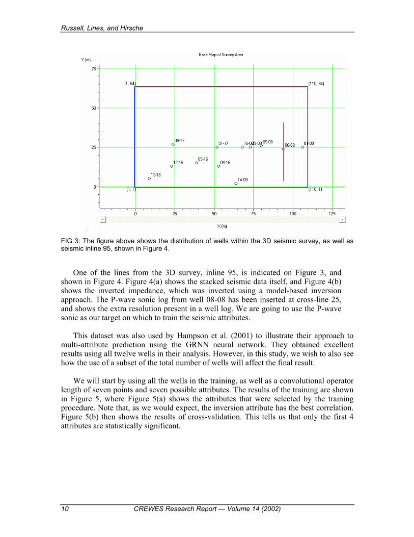
as discussed earlier by Russell et al. (2001). This study involved the prediction of porosity in the Blackfoot field of central Alberta. A 3C-3D seismic survey was recorded in October 1995, with the primary target being the Glauconitic member of the Mannville group. The reservoir occurs at a depth of around 1550 m, where Glauconitic sand and shale fill valleys incised into the regional Mannville stratigraphy. The objectives of the survey were to delineate the channel and distinguish between sand-fill and shale-fill. The well log input consisted of twelve wells, each with sonic, density, and calculated porosity logs, shown in Figure 3.



FIG 3: The figure above shows the distribution of wells within the 3D seismic survey, as well as seismic inline 95, shown in Figure 4.

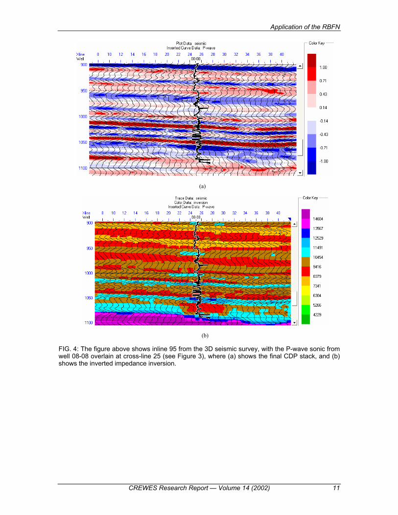
One of the lines from the 3D survey, inline 95, is indicated on Figure 3, and

shown in Figure 4. Figure 4(a) shows the stacked seismic data itself, and Figure 4(b) shows the inverted impedance, which was inverted using a model-based inversion approach. The P-wave sonic log from well 08-08 has been inserted at cross-line 25, and shows the extra resolution present in a well log. We are going to use the P-wave sonic as our target on which to train the seismic attributes.

This dataset was also used by Hampson et al. (2001) to illustrate their approach to

multi-attribute prediction using the GRNN neural network. They obtained excellent results using all twelve wells in their analysis. However, in this study, we wish to also see how the use of a subset of the total number of wells will affect the final result.

We will start by using all the wells in the training, as well as a convolutional operator

length of seven points and seven possible attributes. The results of the training are shown in Figure 5, where Figure 5(a) shows the attributes that were selected by the training procedure. Note that, as we would expect, the inversion attribute has the best correlation. Figure 5(b) then shows the results of cross-validation. This tells us that only the first 4 attributes are statistically significant.



(a)

(b)

FIG. 4: The figure above shows inline 95 from the 3D seismic survey, with the P-wave sonic from well 08-08 overlain at cross-line 25 (see Figure 3), where (a) shows the final CDP stack, and (b) shows the inverted impedance inversion.



(a)

(b)

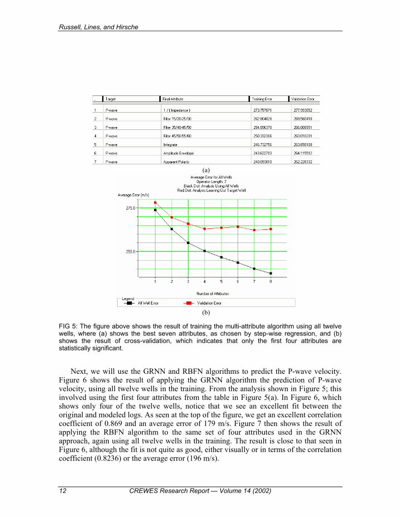
FIG 5: The figure above shows the result of training the multi-attribute algorithm using all twelve wells, where (a) shows the best seven attributes, as chosen by step-wise regression, and (b) shows the result of cross-validation, which indicates that only the first four attributes are statistically significant.

Next, we will use the GRNN and RBFN algorithms to predict the P-wave velocity.

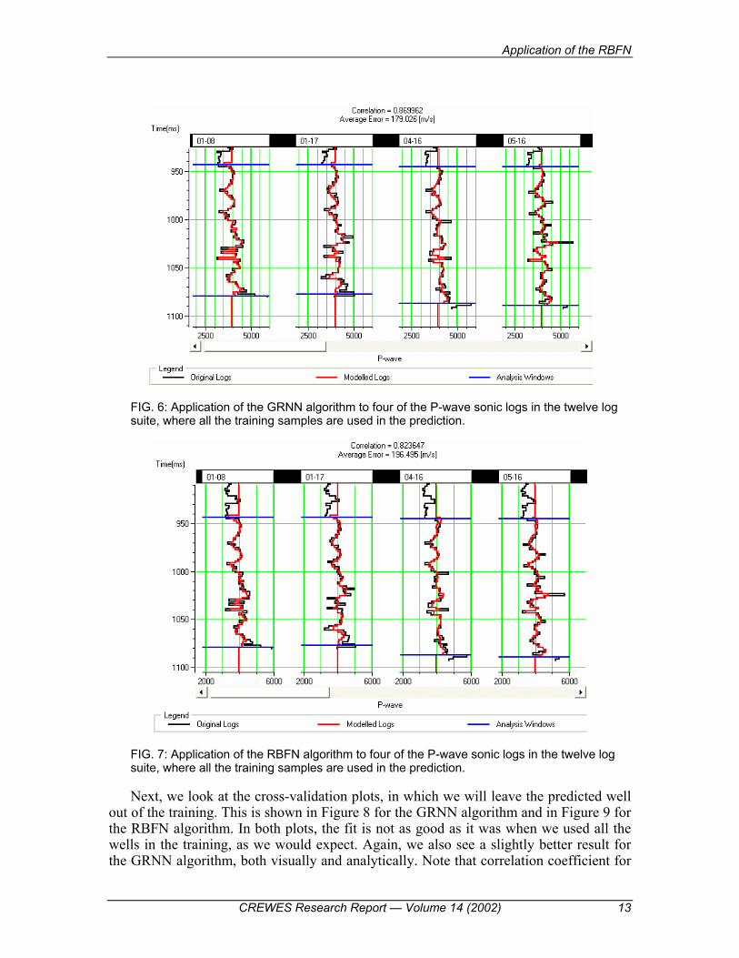
Figure 6 shows the result of applying the GRNN algorithm the prediction of P-wave velocity, using all twelve wells in the training. From the analysis shown in Figure 5; this involved using the first four attributes from the table in Figure 5(a). In Figure 6, which shows only four of the twelve wells, notice that we see an excellent fit between the original and modeled logs. As seen at the top of the figure, we get an excellent correlation coefficient of 0.869 and an average error of 179 m/s. Figure 7 then shows the result of applying the RBFN algorithm to the same set of four attributes used in the GRNN approach, again using all twelve wells in the training. The result is close to that seen in Figure 6, although the fit is not quite as good, either visually or in terms of the correlation coefficient (0.8236) or the average error (196 m/s).



FIG. 6: Application of the GRNN algorithm to four of the P-wave sonic logs in the twelve log suite, where all the training samples are used in the prediction.

FIG. 7: Application of the RBFN algorithm to four of the P-wave sonic logs in the twelve log suite, where all the training samples are used in the prediction.

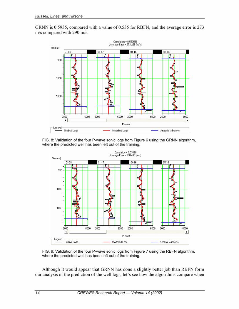
Next, we look at the cross-validation plots, in which we will leave the predicted well

out of the training. This is shown in Figure 8 for the GRNN algorithm and in Figure 9 for the RBFN algorithm. In both plots, the fit is not as good as it was when we used all the wells in the training, as we would expect. Again, we also see a slightly better result for the GRNN algorithm, both visually and analytically. Note that correlation coefficient for



GRNN is 0.5935, compared with a value of 0.535 for RBFN, and the average error is 273 m/s compared with 290 m/s.

FIG. 8: Validation of the four P-wave sonic logs from Figure 6 using the GRNN algorithm, where the predicted well has been left out of the training.

FIG. 9: Validation of the four P-wave sonic logs from Figure 7 using the RBFN algorithm, where the predicted well has been left out of the training.

Although it would appear that GRNN has done a slightly better job than RBFN form our analysis of the prediction of the well logs, let�s see how the algorithms compare when



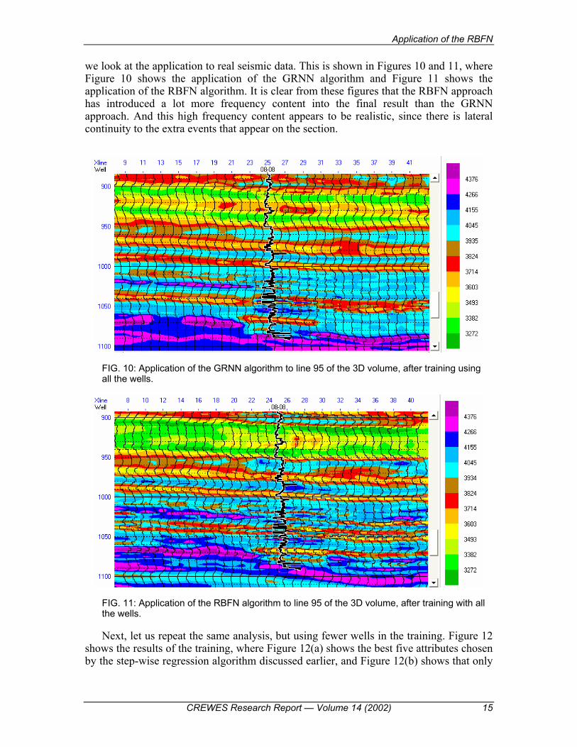
we look at the application to real seismic data. This is shown in Figures 10 and 11, where Figure 10 shows the application of the GRNN algorithm and Figure 11 shows the application of the RBFN algorithm. It is clear from these figures that the RBFN approach has introduced a lot more frequency content into the final result than the GRNN approach. And this high frequency content appears to be realistic, since there is lateral continuity to the extra events that appear on the section.

FIG. 10: Application of the GRNN algorithm to line 95 of the 3D volume, after training using all the wells.

FIG. 11: Application of the RBFN algorithm to line 95 of the 3D volume, after training with all the wells. Next, let us repeat the same analysis, but using fewer wells in the training. Figure 12

shows the results of the training, where Figure 12(a) shows the best five attributes chosen by the step-wise regression algorithm discussed earlier, and Figure 12(b) shows that only



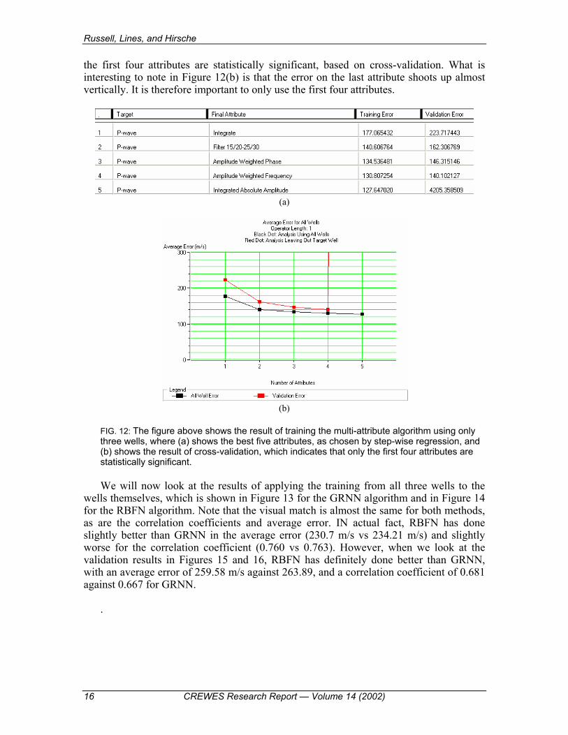
the first four attributes are statistically significant, based on cross-validation. What is interesting to note in Figure 12(b) is that the error on the last attribute shoots up almost vertically. It is therefore important to only use the first four attributes.

(a)

(b)

FIG. 12: The figure above shows the result of training the multi-attribute algorithm using only three wells, where (a) shows the best five attributes, as chosen by step-wise regression, and (b) shows the result of cross-validation, which indicates that only the first four attributes are statistically significant.

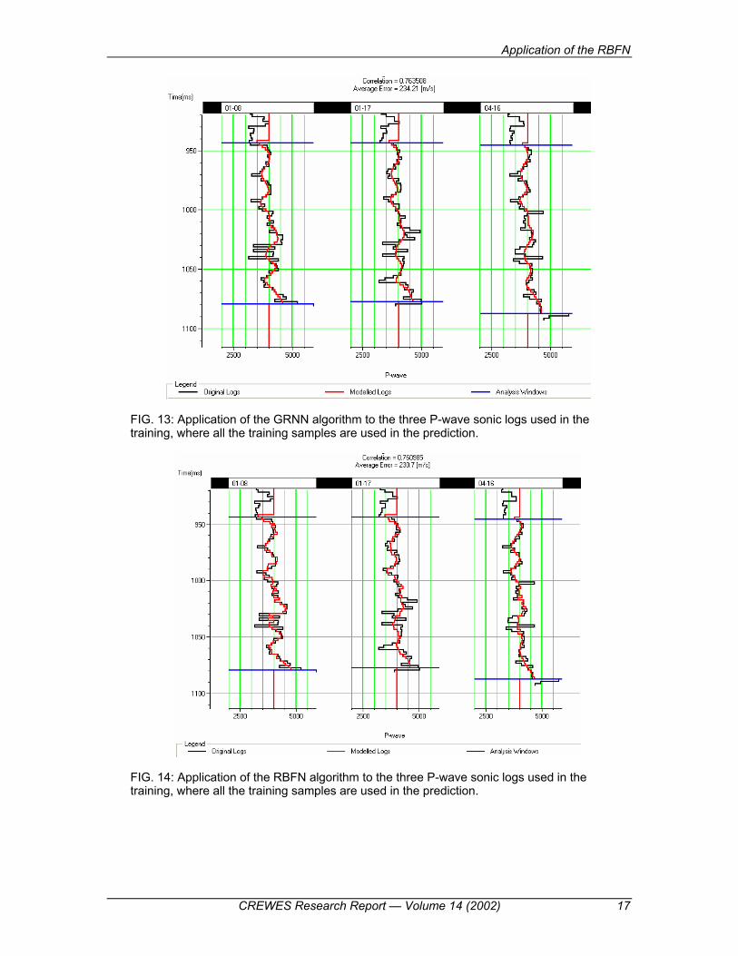
We will now look at the results of applying the training from all three wells to the

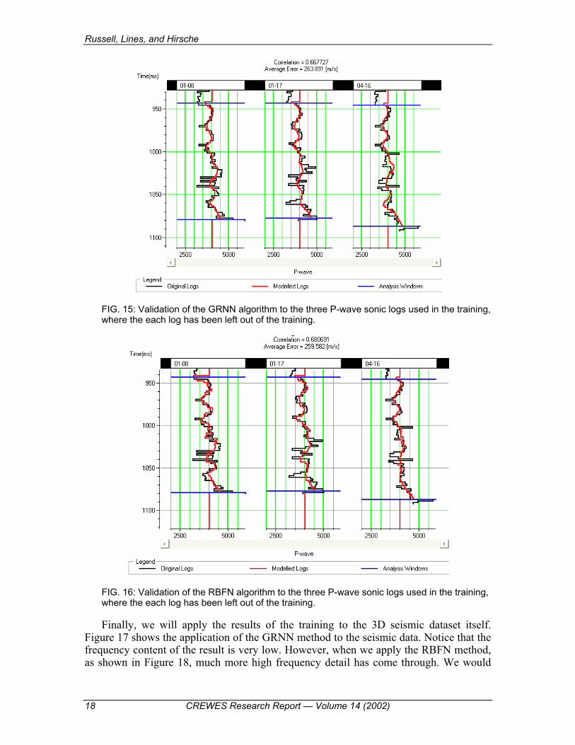
wells themselves, which is shown in Figure 13 for the GRNN algorithm and in Figure 14 for the RBFN algorithm. Note that the visual match is almost the same for both methods, as are the correlation coefficients and average error. IN actual fact, RBFN has done slightly better than GRNN in the average error (230.7 m/s vs 234.21 m/s) and slightly worse for the correlation coefficient (0.760 vs 0.763). However, when we look at the validation results in Figures 15 and 16, RBFN has definitely done better than GRNN, with an average error of 259.58 m/s against 263.89, and a correlation coefficient of 0.681 against 0.667 for GRNN.

.



FIG. 13: Application of the GRNN algorithm to the three P-wave sonic logs used in the training, where all the training samples are used in the prediction.

FIG. 14: Application of the RBFN algorithm to the three P-wave sonic logs used in the training, where all the training samples are used in the prediction.



FIG. 15: Validation of the GRNN algorithm to the three P-wave sonic logs used in the training, where the each log has been left out of the training.

FIG. 16: Validation of the RBFN algorithm to the three P-wave sonic logs used in the training, where the each log has been left out of the training.

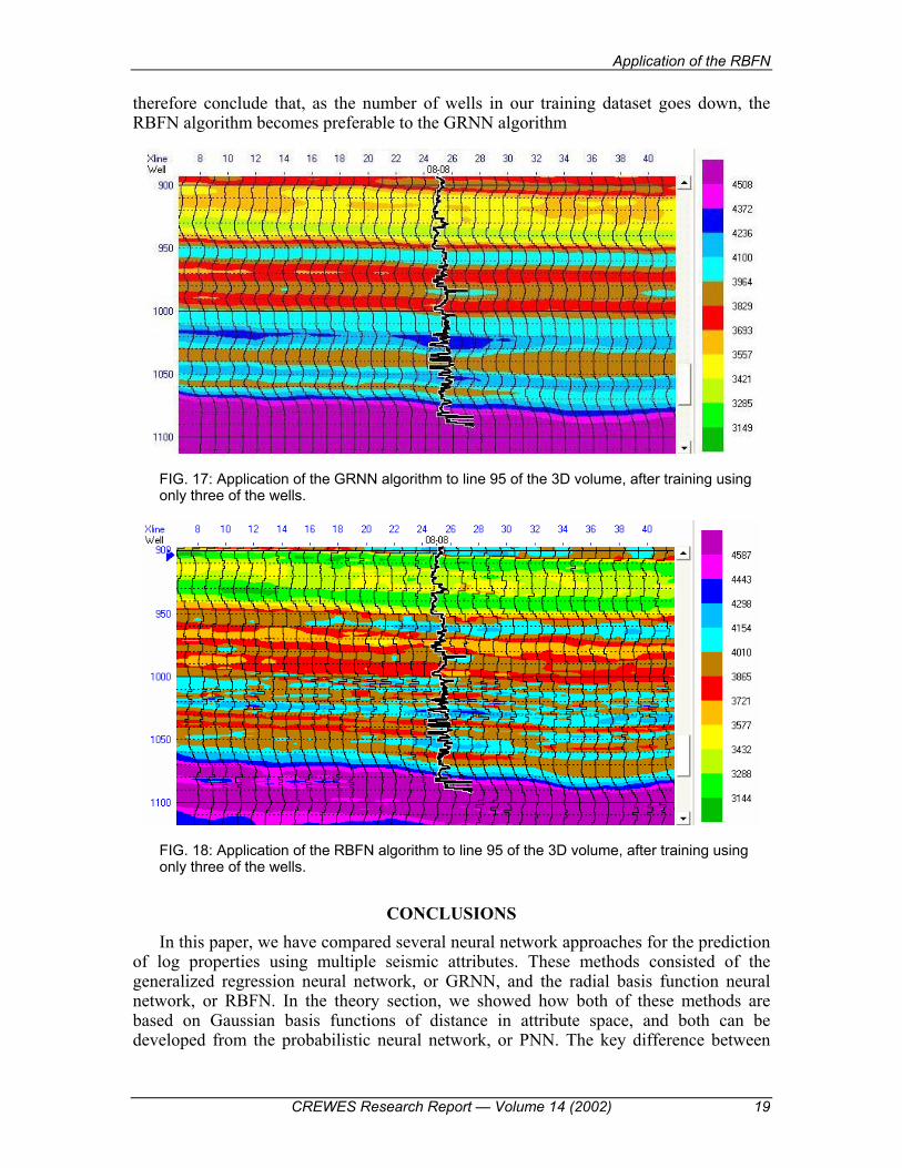
Finally, we will apply the results of the training to the 3D seismic dataset itself.

Figure 17 shows the application of the GRNN method to the seismic data. Notice that the frequency content of the result is very low. However, when we apply the RBFN method, as shown in Figure 18, much more high frequency detail has come through. We would



therefore conclude that, as the number of wells in our training dataset goes down, the RBFN algorithm becomes preferable to the GRNN algorithm

FIG. 17: Application of the GRNN algorithm to line 95 of the 3D volume, after training using only three of the wells.

FIG. 18: Application of the RBFN algorithm to line 95 of the 3D volume, after training using only three of the wells.

CONCLUSIONS

In this paper, we have compared several neural network approaches for the prediction of log properties using multiple seismic attributes. These methods consisted of the generalized regression neural network, or GRNN, and the radial basis function neural network, or RBFN. In the theory section, we showed how both of these methods are based on Gaussian basis functions of distance in attribute space, and both can be developed from the probabilistic neural network, or PNN. The key difference between



GRNN and RBFN is that the GRNN prediction is a weighted sum of the basis functions and the training values, whereas in the RBFN the weights are pre-computed using a generalized matrix inversion of the basis functions weighted by the training values.

After a discussion of the methodology used in finding the best set of attributes, and

those attributes that are statistically significant, we applied the two methods to a channel sand case study from Alberta. We first did the training using all twelve wells in the study area. The results of the training showed the GRNN was marginally better than RBFN in predicting the well log values, both using all the training wells and in the cross-validation tests. This was quantified by looking at the training error and correlation coefficient values. However, when we applied the training to the seismic dataset, the RBFN method produced high frequency results than the GRNN method, with good lateral continuity.

We then applied the methods using only three of the wells in the training phase, the

results were different. In this case, the RBFN method was quantitatively better than the GRNN method, for both the full application and cross-validation results. That is, the training error was smaller and correlation coefficient larger. The effect on the seismic data was even more dramatic. The application of the RBFN method displayed much higher frequency content on the seismic data than the application of the GRNN method.

Our conclusion is therefore that, as the number of wells in the training dataset goes

down, RBFN provides a better technique for predicting log properties from seismic attributes, both in the fit at the training wells and in the application to the seismic. As the number of wells increases, the two methods produce fairly consistent results, with GRNN doing a slightly better job of predicting the training wells, and RBFN doing a better job of brining out the high frequencies in the seismic data.

FUTURE WORK

Future work will involve research into alternate forms of neural networks that can be applied to this problem, and a search for a faster algorithm to solve for the optimum sigma value in the RBFN method.

ACKNOWLEDGEMENTS

We wish to thank our colleagues at the CREWES Project and at Hampson-Russell Software for their support and ideas, as well as the sponsors of the CREWES Project.

REFERENCES Bishop, C.M., 1995, Neural Networks for Pattern Recognition: Oxford University Press, Oxford, UK.

Hampson, D., Schuelke, J.S., and Quirein, J.A., 2001, Use of multiattribute transforms to predict log properties from seismic data: Geophysics, 66, 220-231. Kohonen, T., 2001, Self Organizing Maps: Springer Series in Information Sciences, 20, Springer Verlag, Berlin. Masters, T., 1995, Advance Algorithms for Neural Networks, John Wiley and Sons, Inc. Nadaraya, E.A., 1964, On estimating regression: Theory of Probability and its Applications 9 (1), 55-59.



Poggio, T., and Girosi, F., 1990, Networks for approximation and learning: Proceedings of the IEEE 78 (9), 1481-1497. Powell, M.J.D., 1987, Radial basis functions for multivariable interpolation: a review. In J.C. Mason and M.G. Cox (Eds.), Algorithms for Approximation, 143-167. Oxford: Clarendon Press.

Ronen, S., Schultz, P.S., Hattori, M., and Corbett, C., 1994, Seismic-guided estimation of log properties, Parts 1, 2, and 3: The Leading Edge, 13, 305-310, 674-678, and 770-776. Russell, B., Hampson D.P., Lines L.R., and Todorov, T., 2001 Combining geostatistics and multiattribute transforms � A channel sand case study, CREWES Research Report 13, 827-842.

Russell, B.H, Lines, L.R., and Ross, C.P., 2002, AVO classification using neural networks: A comparison of two methods: CREWES Research Report 14, this volume. Specht, D.F., 1990, Probabilistic neural networks: Neural Networks 3 (1), 109-118. Taner, M. T., Koehler, F. and Sheriff, R. E., 1979, Complex seismic trace analysis: Geophysics, 44, 1041-1063. Watson, G.S., 1964, Smooth regression analysis: Sankhya, the Indian Journal of Statistics. Series A 26, 359-372.

Documents

Application of the radial basis function neural network to ... · Application of the RBFN CREWES Research Report Š Volume 14 (2002) 1 Application of the radial basis function neural