NEURAL NETWORKS AND THE NATURAL GRADIENT by · Neural Networks and the Natural Gradient by ... C.1 Ordinary Gradient Learning ... 1.10 The plot of the output of a double-layer perceptron

NEURAL NETWORKS AND THE NATURAL GRADIENT

by

Michael R. Bastian

A dissertation submitted in partial fulfillmentof the requirements for the degree

of

DOCTOR OF PHILOSOPHY

in

Electrical Engineering

Approved:

Dr. Jacob H. Gunther Dr. Todd K. MoonMajor Professor Committee Member

Dr. YangQuan Chen Dr. Wei RenCommittee Member Committee Member

Dr. Donald Cooley Dr. Byron R. BurnhamCommittee Member Dean of Graduate Studies

UTAH STATE UNIVERSITYLogan, Utah

2009

ii

Copyright c© Michael R. Bastian 2009

All Rights Reserved

iii

Abstract

Neural Networks and the Natural Gradient

by

Michael R. Bastian, Doctor of Philosophy

Utah State University, 2009

Major Professor: Dr. Jacob H. GuntherDepartment: Electrical and Computer Engineering

Neural network training algorithms have always suffered from the problem of local

minima. The advent of natural gradient algorithms promised to overcome this shortcoming

by finding better local minima. However, they require additional training parameters and

computational overhead. By using a new formulation for the natural gradient, an algorithm

is described that uses less memory and processing time than previous algorithms with

comparable performance.

(153 pages)

iv

Ad Majorem Dei Gloriam

v

Acknowledgments

I would have not been able to write this dissertation without the help of Dr. Jacob

H. Gunther and Dr. Todd K. Moon. They were both excellent mentors and have vast

knowledge of our discipline. Without their guidance I would not have been able to develop

my research.

My wife has been very patient with me during the last six years while I completed

coursework and developed the ideas in this dissertation. Her encouragement has helped me

complete it. My children have also helped me by giving me time to write.

I would like to thank my other committee members for their valuable input during the

progress of my research. The faculty and staff of the Electrical and Computer Engineering

Deparment have been an excellent resource. I thank you all.

The United States Air Force is my employer and has been very supportive of my efforts

and has allowed me time off to work on my dissertation. The financial support of the USAF

has also allowed me to present my work at two conferences.

Finally, writing this dissertation would have been much more difficult without the

LATEX Companion [1].

Michael R. Bastian

vi

Contents

Page

Abstract . . . . . . . . . . . . . . . . . . . . . . . . . . . . . . . . . . . . . . . . . . . . . . . . . . . . . . . iii

Acknowledgments . . . . . . . . . . . . . . . . . . . . . . . . . . . . . . . . . . . . . . . . . . . . . . . v

List of Tables . . . . . . . . . . . . . . . . . . . . . . . . . . . . . . . . . . . . . . . . . . . . . . . . . . . ix

List of Figures . . . . . . . . . . . . . . . . . . . . . . . . . . . . . . . . . . . . . . . . . . . . . . . . . . x

Notation . . . . . . . . . . . . . . . . . . . . . . . . . . . . . . . . . . . . . . . . . . . . . . . . . . . . . . . xiii

Acronyms . . . . . . . . . . . . . . . . . . . . . . . . . . . . . . . . . . . . . . . . . . . . . . . . . . . . . . xiv

1 Introduction to Artificial Neural Networks . . . . . . . . . . . . . . . . . . . . . . . . 11.1 Historical Development . . . . . . . . . . . . . . . . . . . . . . . . . . . . . 11.2 Biological Background . . . . . . . . . . . . . . . . . . . . . . . . . . . . . . 11.3 Basic Computational Structure . . . . . . . . . . . . . . . . . . . . . . . . . 2

1.3.1 Parameters of an Artificial Neuron . . . . . . . . . . . . . . . . . . . 31.3.2 Sigmoid Functions . . . . . . . . . . . . . . . . . . . . . . . . . . . . 31.3.3 Linear Classifiers . . . . . . . . . . . . . . . . . . . . . . . . . . . . . 31.3.4 Training an Artificial Neuron . . . . . . . . . . . . . . . . . . . . . . 51.3.5 Online and Batch Training . . . . . . . . . . . . . . . . . . . . . . . 91.3.6 Avoiding Overtraining . . . . . . . . . . . . . . . . . . . . . . . . . . 101.3.7 Newton’s Method . . . . . . . . . . . . . . . . . . . . . . . . . . . . . 121.3.8 Annealed Learning Rates . . . . . . . . . . . . . . . . . . . . . . . . 161.3.9 Criticism of Neurons and Linear Classifiers . . . . . . . . . . . . . . 16

1.4 Multilayer Perceptrons . . . . . . . . . . . . . . . . . . . . . . . . . . . . . . 181.4.1 The Linear Perceptron . . . . . . . . . . . . . . . . . . . . . . . . . . 181.4.2 Nonlinear Perceptrons . . . . . . . . . . . . . . . . . . . . . . . . . . 191.4.3 Perceptron Composition . . . . . . . . . . . . . . . . . . . . . . . . . 201.4.4 Learning the XOR Function . . . . . . . . . . . . . . . . . . . . . . . 211.4.5 The Backpropagation of Error . . . . . . . . . . . . . . . . . . . . . 28

1.5 Radial Basis Function Networks . . . . . . . . . . . . . . . . . . . . . . . . . 291.5.1 An Example Radial Basis Function Network . . . . . . . . . . . . . . 301.5.2 Training a Radial Basis Function Network . . . . . . . . . . . . . . . 30

1.6 Conclusion . . . . . . . . . . . . . . . . . . . . . . . . . . . . . . . . . . . . 32

2 Simplified Natural Gradient . . . . . . . . . . . . . . . . . . . . . . . . . . . . . . . . . . . . 332.1 Natural Gradient . . . . . . . . . . . . . . . . . . . . . . . . . . . . . . . . . 33

2.1.1 A Probabilistic Model . . . . . . . . . . . . . . . . . . . . . . . . . . 342.1.2 Sufficient Statistics . . . . . . . . . . . . . . . . . . . . . . . . . . . . 352.1.3 The Exponential Family . . . . . . . . . . . . . . . . . . . . . . . . . 37

vii

2.1.4 Optimal Parameter Estimation . . . . . . . . . . . . . . . . . . . . . 372.1.5 The Fisher Information . . . . . . . . . . . . . . . . . . . . . . . . . 382.1.6 The Geometry of Exponential Families . . . . . . . . . . . . . . . . . 402.1.7 Direction of Steepest Descent . . . . . . . . . . . . . . . . . . . . . . 41

2.2 Amari’s Adaptive Natural Gradient for Multilayer Perceptrons . . . . . . . 422.3 Algebraic Structure of Multilayer Perceptrons . . . . . . . . . . . . . . . . . 42

2.3.1 Directional Derivative . . . . . . . . . . . . . . . . . . . . . . . . . . 432.3.2 The Fisher Information Matrix of a Single-Layer Perceptron . . . . . 462.3.3 The Fisher Information Matrix of a Multilayer Perceptron . . . . . . 48

2.4 Simplified Natural Gradient Example . . . . . . . . . . . . . . . . . . . . . . 502.5 Adding a Prior Distribution with a Hyperparameter . . . . . . . . . . . . . 522.6 Conclusion . . . . . . . . . . . . . . . . . . . . . . . . . . . . . . . . . . . . 54

3 Experimental Results . . . . . . . . . . . . . . . . . . . . . . . . . . . . . . . . . . . . . . . . . . 553.1 Effective Learning Rate . . . . . . . . . . . . . . . . . . . . . . . . . . . . . 563.2 Exclusive OR Problem (XOR) . . . . . . . . . . . . . . . . . . . . . . . . . 56

3.2.1 The Eigenvalues of the Fisher Information Matrix . . . . . . . . . . 573.2.2 Performance Comparison . . . . . . . . . . . . . . . . . . . . . . . . 57

3.3 Low-Density Parity Check (LDPC) Code . . . . . . . . . . . . . . . . . . . 643.3.1 Performance Comparison . . . . . . . . . . . . . . . . . . . . . . . . 663.3.2 The Effective Learning Rate . . . . . . . . . . . . . . . . . . . . . . . 673.3.3 Substituting Learning Rates . . . . . . . . . . . . . . . . . . . . . . . 67

3.4 The Iris Species Identification Problem . . . . . . . . . . . . . . . . . . . . . 703.4.1 Probabilistic Model . . . . . . . . . . . . . . . . . . . . . . . . . . . 723.4.2 Performance Comparison . . . . . . . . . . . . . . . . . . . . . . . . 74

3.5 Mackey-Glass Time Series Prediction Problem . . . . . . . . . . . . . . . . . 743.5.1 Network Architecture . . . . . . . . . . . . . . . . . . . . . . . . . . 783.5.2 Performance Comparison . . . . . . . . . . . . . . . . . . . . . . . . 78

3.6 Nonlinear Dimension Reduction . . . . . . . . . . . . . . . . . . . . . . . . . 803.6.1 Flattening a Semicircle . . . . . . . . . . . . . . . . . . . . . . . . . . 803.6.2 Locally Linear Embedding . . . . . . . . . . . . . . . . . . . . . . . . 86

3.7 Computational Complexity Comparison . . . . . . . . . . . . . . . . . . . . 903.8 Comparison with Other Optimization Algorithms . . . . . . . . . . . . . . . 91

3.8.1 Line Search . . . . . . . . . . . . . . . . . . . . . . . . . . . . . . . . 913.8.2 Trust Region . . . . . . . . . . . . . . . . . . . . . . . . . . . . . . . 94

3.9 Normalizing the Error Gradient . . . . . . . . . . . . . . . . . . . . . . . . . 963.10 Conclusion . . . . . . . . . . . . . . . . . . . . . . . . . . . . . . . . . . . . 99

4 Summary and Future Work . . . . . . . . . . . . . . . . . . . . . . . . . . . . . . . . . . . . . 1004.1 Research Summary . . . . . . . . . . . . . . . . . . . . . . . . . . . . . . . . 1004.2 Contributions . . . . . . . . . . . . . . . . . . . . . . . . . . . . . . . . . . . 1014.3 Future Work . . . . . . . . . . . . . . . . . . . . . . . . . . . . . . . . . . . 1014.4 Conclusion . . . . . . . . . . . . . . . . . . . . . . . . . . . . . . . . . . . . 102

References . . . . . . . . . . . . . . . . . . . . . . . . . . . . . . . . . . . . . . . . . . . . . . . . . . . . . . 103

viii

Appendices . . . . . . . . . . . . . . . . . . . . . . . . . . . . . . . . . . . . . . . . . . . . . . . . . . . . . 107Appendix A MATLAB Code for the Exclusive OR (XOR) Experiment . . . . 108A.1 Ordinary Gradient Learning . . . . . . . . . . . . . . . . . . . . . . . . . . . 108A.2 Simplified Natural Gradient Learning . . . . . . . . . . . . . . . . . . . . . . 110A.3 Adaptive Natural Gradient Learning . . . . . . . . . . . . . . . . . . . . . . 112Appendix B MATLAB Code for the Low-Density Parity Check Code Experiment115B.1 Ordinary Gradient Learning . . . . . . . . . . . . . . . . . . . . . . . . . . . 115B.2 Simplified Natural Gradient Learning . . . . . . . . . . . . . . . . . . . . . . 117B.3 Adaptive Natural Gradient Learning . . . . . . . . . . . . . . . . . . . . . . 119Appendix C MATLAB Code for the Fisher’s Iris Data Experiment . . . . . . . 121C.1 Ordinary Gradient Learning . . . . . . . . . . . . . . . . . . . . . . . . . . . 125C.2 Simplified Natural Gradient Learning . . . . . . . . . . . . . . . . . . . . . . 127C.3 Adaptive Natural Gradient Learning . . . . . . . . . . . . . . . . . . . . . . 129Appendix D MATLAB Code for the Mackey-Glass Chaotic Time Series Exper-

iment . . . . . . . . . . . . . . . . . . . . . . . . . . . . . . . . . . . . . . . 131D.1 Ordinary Gradient Learning . . . . . . . . . . . . . . . . . . . . . . . . . . . 132D.2 Simplified Natural Gradient Learning . . . . . . . . . . . . . . . . . . . . . . 133D.3 Adaptive Natural Gradient Learning . . . . . . . . . . . . . . . . . . . . . . 134Appendix E MATLAB Code for the Semicircle and S-Curve Unfolding Experi-

ments . . . . . . . . . . . . . . . . . . . . . . . . . . . . . . . . . . . . . . . 135E.1 Ordinary Gradient Learning . . . . . . . . . . . . . . . . . . . . . . . . . . . 136E.2 Simplified Natural Gradient Learning . . . . . . . . . . . . . . . . . . . . . . 137E.3 Adaptive Natural Gradient Learning . . . . . . . . . . . . . . . . . . . . . . 138

Vita . . . . . . . . . . . . . . . . . . . . . . . . . . . . . . . . . . . . . . . . . . . . . . . . . . . . . . . . . . . 139

ix

List of Tables

Table Page

3.1 The results of and parameters used for the OGL, SNGL, and ANGL algo-rithms on the XOR problem. . . . . . . . . . . . . . . . . . . . . . . . . . . 61

3.2 LDPC experiment results. . . . . . . . . . . . . . . . . . . . . . . . . . . . . 68

3.3 Fisher’s iris data experiment results. . . . . . . . . . . . . . . . . . . . . . . 75

3.4 Mackey-Glass experiment results. . . . . . . . . . . . . . . . . . . . . . . . . 81

3.5 Nonlinear dimension reduction experiment results. . . . . . . . . . . . . . . 84

3.6 Locally linear embedding results. . . . . . . . . . . . . . . . . . . . . . . . . 87

3.7 Comparison between the computational complexity of the SNGL and ANGLalgorithms in both space and time. . . . . . . . . . . . . . . . . . . . . . . . 90

x

List of Figures

Figure Page

1.1 The basic anatomy of the neuron. The soma is the body of the neuron cell.The dendrites receive signals through the synapses. The axon connects toother synapses. . . . . . . . . . . . . . . . . . . . . . . . . . . . . . . . . . . 2

1.2 The logistic curve. . . . . . . . . . . . . . . . . . . . . . . . . . . . . . . . . 4

1.3 The blue circles are the positive examples and the green x’s are the negativeexamples. The red line is the decision boundary of the linear classifier. . . . 6

1.4 The effect of overtraining is shown as the gain of the input to a sigmoidfunction increases. The slope of the line increases and the curvature at thesaturation level also increases. . . . . . . . . . . . . . . . . . . . . . . . . . . 11

1.5 The derivative of the logistic function. . . . . . . . . . . . . . . . . . . . . . 15

1.6 The learning rate is flat for the first hundred epochs and then decays withthe inverse of the learning epoch index. . . . . . . . . . . . . . . . . . . . . 17

1.7 The points of XOR problem space and their separating lines x1 − x2 − 1 = 0and x2 − x1 − 1 = 0. . . . . . . . . . . . . . . . . . . . . . . . . . . . . . . . 23

1.8 The first affine transformation maps both (−1,−1) and (+1,+1) to (−1,−1).The mapping of all the training points lie on the same line: x1 + x2 = −2. . 24

1.9 The transfer function warps the points so that the line x1+x2 = −1 separatesthe positive example from the negative ones. . . . . . . . . . . . . . . . . . 26

1.10 The plot of the output of a double-layer perceptron that computes the XORfunction. . . . . . . . . . . . . . . . . . . . . . . . . . . . . . . . . . . . . . . 27

2.1 The map of the Earth drawn by Gerardus Mercator in 1569. . . . . . . . . . 35

3.1 This plot shows the labeling of the XOR problem. The red correspond to anoutput value of 1 and the blue to a value of -1. . . . . . . . . . . . . . . . . 58

3.2 This plot shows the eigenvalues of the Fisher information matrix for eachlearning epoch. The Fisher information is a metric for the variance of theparameters around the current estimate. High variance means that theremore information to be gleaned from the data into the parameters. . . . . . 59

xi

3.3 The sum-squared error curves of OGL, ANGL, and SNGL with effectivelearning rate η = 0.25 and SNGL modified to use an annealed learning rate. 61

3.4 The effective learning rates of the OGL, SNGL, and ANGL algorithms forthe XOR problem. . . . . . . . . . . . . . . . . . . . . . . . . . . . . . . . . 63

3.5 The SSE of the SNGL algorithm for the XOR problem with the two valuesfor learning rate and hyperparameters. . . . . . . . . . . . . . . . . . . . . . 65

3.6 Sum-squared error of the Ordinary Gradient Learning (OGL), Simplified Nat-ural Gradient Learning (SNGL), and Adaptive Natural Gradient Learning(ANGL) algorithms when learning the rate 1/2 (10,5) low-density paritycheck encoding function with G as its generator matrix. . . . . . . . . . . . 68

3.7 Effective learning rate of the OGL, SNGL, and ANGL algorithms when learn-ing the LDPC encoding function. . . . . . . . . . . . . . . . . . . . . . . . . 69

3.8 Sum-squared error of the OGL, SNGL, and ANGL algorithms compared tothe OGL algorithm with the effective LR of the ANGL and SNGL algorithms. 71

3.9 Sum-squared error of the OGL, ANGL, and SNGL algorithms on Fisher’siris data. . . . . . . . . . . . . . . . . . . . . . . . . . . . . . . . . . . . . . . 75

3.10 The number of misclassified test case of the OGL, ANGL, and SNGL algo-rithms on Fisher’s iris data. . . . . . . . . . . . . . . . . . . . . . . . . . . . 76

3.11 The effective learning rate of the OGL, ANGL, and SNGL algorithms onFisher’s iris data. . . . . . . . . . . . . . . . . . . . . . . . . . . . . . . . . . 77

3.12 The training set of the Mackey-Glass time series prediction problem. . . . . 79

3.13 The sum-squared error of the OGL, ANGL, and SNGL algorithms on theMackey-Glass time series prediction problem. . . . . . . . . . . . . . . . . . 81

3.14 The effective learning rate of the OGL, ANGL, and SNGL algorithms on theMackey-Glass time series prediction problem. . . . . . . . . . . . . . . . . . 82

3.15 An instance of 100 points on the semicircle between π6 and 11π

6 that has beencorrupted by additive white Gaussian noise with σ = 0.1. . . . . . . . . . . 84

3.16 The sum-squared error of the for the OGL, SNGL, and ANGL algorithmslearning the noisy semicircle unfolding problem. . . . . . . . . . . . . . . . . 85

3.17 The effective learning rate of the OGL, SNGL, and ANGL algorithms on thenoisy semicircle unfolding Problem. . . . . . . . . . . . . . . . . . . . . . . . 87

3.18 The S-curve manifold, a set of sampled data and its image under a locallylinear embedding map. . . . . . . . . . . . . . . . . . . . . . . . . . . . . . . 88

xii

3.19 The sum-squared error of the for the OGL, SNGL, and ANGL algorithms onthe S-curve problem. . . . . . . . . . . . . . . . . . . . . . . . . . . . . . . . 88

3.20 The effective learning rate of the OGL, SNGL, and ANGL algorithms on thenoisy semicircle unfolding problem. . . . . . . . . . . . . . . . . . . . . . . . 89

3.21 The sum-squared error of the for the OGL, SNGL, ANGL, and Line SearchMethod (LSM) algorithms on the noisy semicircle unfolding problem. . . . . 93

3.22 The effective learning rate of the OGL, SNGL, ANGL, and Line SearchMethod (LSM) algorithms on the noisy semicircle unfolding problem. . . . . 95

3.23 The sum-squared error of the for the OGL, SNGL, ANGL, Line SearchMethod (LSM), and Trust Region Method (TRM) algorithms on the noisysemicircle unfolding problem. . . . . . . . . . . . . . . . . . . . . . . . . . . 97

3.24 The value of the parameter τ used in the trust region method algorithm onthe noisy semicircle unfolding problem. . . . . . . . . . . . . . . . . . . . . . 98

xiii

Notation

a A scalar value

f(x) A real-valued function of x

X A random variable

x A vector

〈x,y〉 The inner product of x and y

‖x‖ The norm of x

A A matrix

X A random vector

F(x) A real vector-valued function of the vector x

AT The transpose of the matrix A

tr(A) Trace of the matrix A

E{X} The expected value of of the random variable X

xiv

Acronyms

ANGL Adaptive Natural Gradient Learning (Multilayer Perceptron)

BFGS Broyden, Fletcher, et al. Optimization Algorithm

BSS Blind Source Separation

CDF Cumulative Distribution Function

FIM Fisher Information Matrix

ICA Independent Component Analysis

LM Levenburg-Marquardt Optimization Algorithm

LR Learning Rate

LSM Line Search Method

MAP Maximum A Posteriori

ML Maximum Likelihood

MLP Multilayer Perceptron

NG Natural Gradient

OGL Ordinary Gradient Learning (Multilayer Perceptron)

PDF Probability Density Function

RBF Radial Basis Function

RVM Relevance Vector Machine

SVM Support Vector Machine

XOR Exclusive-OR

1

Chapter 1

Introduction to Artificial Neural Networks

This dissertation is about training artificial neural networks with natural gradient al-

gorithms. Knowledge of the basics of neural networks is necessary to understand the devel-

opments in this dissertation. Thus, this first chapter is a gentle introduction to the field of

artificial neural networks and machine learning.

1.1 Historical Development

The discipline of artificial intelligence began with Huxley’s hypothesis that animal

behavior could be explained with automata [2]. This caused William James to ask the

question, “Are we automata?” five years later [3]. However, these two essays are purely

philosophical. The first scientific development linking human ideas and eletrical impulses in

the brain was reported by McColluch and Pitts [4]. Further evidence was found by Hebb [5].

These ideas combined with the development of Turing Machines [6–8] laid the physical and

mathematical foundations for the development of neural networks.

1.2 Biological Background

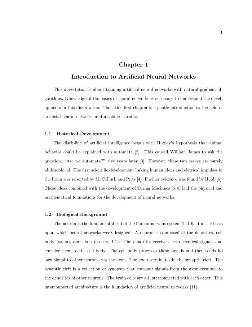
The neuron is the fundamental cell of the human nervous system [9,10]. It is the basis

upon which neural networks were designed. A neuron is composed of the dendrites, cell

body (soma), and axon (see fig. 1.1). The dendrites receive electrochemical signals and

transfer them to the cell body. The cell body processes these signals and then sends its

own signal to other neurons via the axon. The axon terminates in the synaptic cleft. The

synaptic cleft is a collection of synapses that transmit signals from the axon terminal to

the dendrites of other neurons. The brain cells are all interconnected with each other. This

interconnected architecture is the foundation of artificial neural networks [11].

2

Fig. 1.1: The basic anatomy of the neuron. The soma is the body of the neuron cell. Thedendrites receive signals through the synapses. The axon connects to other synapses.

Neurons react to the stimuli they receive from the synapses connected to their dendrites.

When a neuron is near its unexcited state and the impulses increase or decrease in voltage,

the electrical response from the neuron is nearly linear to its input. However, there is

a threshold in its response that it does not exceed. Its response gradually tapers off as

the magnitude of the voltage increases. When it reaches this limit the neuron is in a

saturated state. This trait is mimicked by artificial neurons. The biological inspiration of

artificial neural networks is the interconnected collection of neurons with limited responses

to stimuli [4, 5].

1.3 Basic Computational Structure

Artificial neural networks are composed of artificial neurons that mimic the behavior

of a neuron in a limited way [12]. They mimic the saturation behavior of the human

neuron in the brain. Artificial neurons are functions of several variables with two horizontal

asymptotes. A simple definition of an artificial neuron is a function that maps vectors in a

vector space V to the interval [0, 1]. The interval can actually be any interval of the real

line, but [0, 1] and [−1, 1] are frequently chosen.

3

1.3.1 Parameters of an Artificial Neuron

An artificial neuron has a weight vector w = (w1, w2, . . . , wm) and a threshold or bias

b. The weights are analogous to the strength of the dendritic connections. The bias is

considered the value that must be surpassed by the inputs before an artificial neuron will

become active (i.e., greater than zero). However, it is usually written as an additive term.

The activation of a neuron is the sum of the inner product of the weight vector with

an input vector x = (x1, x2, . . . , xm) and the bias:

a =m∑

i=1

wixi + b. (1.1)

The weights and the bias define a hyperplane in the vector space V with dimension n. The

activation of the neuron is the distance of the input vector from this hyperplane.

1.3.2 Sigmoid Functions

The saturation property is achieved by “squashing” the activation of a neuron with a

sigmoid transfer function like

f(t) =1

1 + e−t. (1.2)

This limits the output between 0 and 1. These functions are called sigmoid functions

because of their “S”-shape (see fig. 1.2). The function in (1.2) is the logistic function.

It is the CDF of the Logistic Distribution. Other sigmoid functions are the arctangent,

hyperbolic tangent, and the error function [13].

Another property of the sigmoid function is that their derivatives can be written as

quadratic functions of their values. For example, the derivative of the logistic function

in (1.2) is

f ′(t) =e−t

(1 + e−t)2= f(t)[1− f(t)]. (1.3)

1.3.3 Linear Classifiers

Suppose that there are two finite sets of vectors, X0 and X1, in a vector space V . Any

hyperplane will split V into two distinct subsets, V0 and V1. If X0 ⊂ V0 and X1 ⊂ V1, then

4

Fig. 1.2: The logistic curve.

5

define the probability that a random vector x is in X1 to be the logistic distribution

P [x ∈ X1] =1

1 + exp(−[∑n

i=1wixi + b]) . (1.4)

An artificial neuron is really just a logistic function whose argument is the output of

a linear classifier [12]. The probability that x ∈ X1 increases with the positive distance of

the vector x above the hyperplane. Likewise, this probability decreases with the negative

distance x is below the hyperplane. When the vector x rests on the hyperplane (i.e., the

distance is zero), then the probability P [x ∈ X1] = 0.5. The distance from the hyperplane

is d = 〈x,w〉+ b where w is the normal vector of the hyperplane and b is the distance from

the origin measured in the direction of the normal vector.

An example linear classifier is given in fig. 1.3. The positive examples of the class in

X1 are 100 random vectors from a normal distribution with µ1 = (1.5, 0.5) and σ2 = 0.01.

The negative examples are 100 random vectors from a similar normal distribution with

µ0 = (0.5,−0.5). The decision boundary is the line x1 + x2 = 1.

The neuron parameters are the normal vector and the distance from the origin. Hence,

w = (1, 1) and b = −1. The vector µ1 is exactly 1 unit away from the decision boundary.

Likewise, the vector µ0 is also exactly 1 unit away from the boundary. Thus,

P [µ1 ∈ X1] = f(1) =1

1 + e−1≈ 0.7311,

and

P [µ0 ∈ X1] = f(−1) =1

1 + e≈ 0.2689.

1.3.4 Training an Artificial Neuron

An artificial neuron can be trained to classify vectors by giving it both positive and

negative examples. The training algorithm will then determine the optimal hyperplane with

which to divide the vector space. The neuron is considered to have “learned” the concept

by adjusting its weights and bias.

6

Fig. 1.3: The blue circles are the positive examples and the green x’s are the negativeexamples. The red line is the decision boundary of the linear classifier.

7

The Training Set

The training set is really two sets: The training examples X = {x1,x2, . . . ,xn} and

the training targets Y = {y1, y2, . . . , yn}, where each yk ∈ {0, 1} is the desired output of the

neuron. The indices match such that yk is the desired output for example xk. Hence, the

positive examples belong to the set X1 = {xk|yk = 1} and the negative examples belong to

the set X0 = {xk|yk = 0}.

Probability of Correct Classification

For a given random vector x and the parameters w and b, the probability of a positive

classification is

P [y = 1|x,w, b] = f(〈x,w〉+ b), (1.5)

where f(·) is the logistic sigmoid function [12]. Similarly, the probability of a correct

classification is

p(y|x,w, b) = [f(〈w,x〉+ b)]y[1− f(〈w,x〉+ b)]1−y. (1.6)

The Objective Function

The goal of a training algorithm is maximize the correct classification of all the training

examples. Formally, that means determine parameters w and b such that

p(y|w, b) =n∏

k=1

[f(〈w,xk〉+ b)]yk [1− f(〈w,xk〉+ b)]1−yk (1.7)

is maximized [14]. An equivalent problem is to minimize the log-likelihood

`(w, b) = log p(y|w, b) (1.8)

=n∑

k=1

yk log(f(〈w,xk〉+ b)) + (1− yk) log(1− f(〈w,xk〉+ b)). (1.9)

8

The Gradient

A gradient ascent algorithm will determine the optimal values of w and b. Let dk =

〈w,xk〉+ b. The derivative of the log-likelihood function ` with respect to the vector w is

∂`

∂w=

n∑k=1

[ykf

′(dk)f(dk)

− (1− yk)f ′(dk)1− f(dk)

]xk (1.10)

=n∑

k=1

[yk(1− f(dk))− (1− yk)f(dk)]xk (1.11)

=n∑

k=1

[yk − f(dk)]xk. (1.12)

Similarly, the derivative of the log-likelihood function with respect to the bias is

∂`

∂b=

n∑k=1

[yk − f(dk)]. (1.13)

The gradient of the neuron is the difference between its output and the designated target

multiplied by its input vector.

The Learning Rule

The final piece of the algorithm is the learning rule. A learning rule defines how

the weights and bias are changed. In a gradient descent algorithm, the learning rule is to

subtract a small multiple η of the gradient vector from the weights and bias. By distributing

the minus sign into the formula for the gradient, the learning rule is

wt+1 = wt − ηt

n∑k=1

[yk − f(〈wt,xk〉+ bt)]xk, (1.14)

bt+1 = bt − ηt

n∑k=1

[yk − f(〈wt,xk〉+ bt)]. (1.15)

The variable η is called the learning rate. It is the step size for the algorithm. It is

determined empirically for each problem. The subscript t for the weights, bias and learning

rate η denotes the current step of the algorithm. The initial weight vector w0 and bias

b0 are chosen randomly from a uniformly distributed random vector and random variable

9

respectively. A common range is [−0.1, 0.1]m for w0 and [−0.1, 0.1] for b0.

In order for this method of finding the optimal weights and bias to be a true algorithm,

there must be stopping criteria with which the algorithm halts with its best solution. A good

solution for a neuron would be one in which most of the training examples were classified

correctly. When the sum of squares of the errors is less than a predetermined tolerance,

then it can be assumed that most of the training examples were classified correctly. Sum

of squares and the sum of absolute values guard against large errors cancelling each other

out in the sum. As an example, if there is a requirement for 90% accuracy (i.e., the output

is 0.9 or greater for each positive example and 0.1 or less for each negative example), then

the maximum error for each training example would be 0.1. Because there are n training

examples a good stopping criteria would be

1n

n∑k=1

[yk − f(〈wt,xk〉+ bt)]2 < 0.01. (1.16)

1.3.5 Online and Batch Training

There are two ways in which the learning rule may be applied. In batch training the

error is calculated for all the patterns in the training set and then applied to the weights

and bias via the learning rule as in (1.14) and (1.15). In online training the learning rule is

applied after each training example. Hence, given that k = t mod m, the online learning

rule for the neuron would be

wt+1 = wt − ηt[yk − f(〈wt,xk〉+ bt)]xk, (1.17)

bt+1 = bt − ηt[yk − f(〈wt,xk〉+ bt)]. (1.18)

There are two terms used quite frequently in online learning applications: learning

cycle and learning epoch. A learning cycle is one step through an algorithm for one training

example. A learning epoch is one full trip through all the training examples (i.e., n learning

cycles where n is the number of training examples). In a batch algorithm a learning cycle

and a learning epoch are essentially the same concept.

10

There has been some investigation into the merits of both online and batch training [14–

19]. However, batch training will be the focus in this work because of the computational

overhead online training imposes on more advanced training algorithms.

1.3.6 Avoiding Overtraining

Overtraining occurs when a training algorithm has been run through an excessive

number of learning epochs. Essentially, when a nearly optimal solution is found, the weights

and bias tend to increase in value with each succeeding training epoch. The neuron comes

closer and closer to responding with one for each positive example and zero with each

negative example. This is undesirable because the transfer is supposed to be linear in an

interval of its domain. The weight value is essentially the slope. As it increases, so does

the slope. The interval of which it is linear shrinks. The neuron is now overconfident in its

classification.

In fig. 1.4 four sigmoid curves are shown. Each is the plot of f(t), f(2t), f(3t), and

f(6t), respectively. As the weights and bias increase the curve tightens. With a sufficiently

large factor the sigmoid begins to approximate a step function.

Suppose that an artificial neuron was being trained on a computer with floating-point

numbers, then there is a number ε > 0 such that 1 + ε = 1 because of limited precision.

For example, with double precision floating-point arithmetic, ε = 2.2204× 10−16. Let tmax

represent the value such that f(tmax) = 1; then tmax = − log(ε) = 36.0437. The neuron

mimics the behavior of a saturated transistor with stimuli of this magnitude.

A trivial method to avoid overtraining is to stop once the training algorithm has con-

verged to a nearly optimal solution. However, defining convergence and “nearly optimal”

depends heavily on the training data used. Early stopping has the same trait as the halting

problem from computer science: How long is long enough?

Adding a prior distribution on the neural parameters w and b that penalizes larger

parameters with smaller probabilities causes the algorithm to essentially stop when the

parameters become large enough, but no larger [12].

11

Fig. 1.4: The effect of overtraining is shown as the gain of the input to a sigmoid functionincreases. The slope of the line increases and the curvature at the saturation level alsoincreases.

12

A Gaussian distribution with density function p(w, b) = exp(−12α[‖w‖2 + b2]) is an

adequate choice. The hyperparameter α controls how big the parameters become. The

relationship between α and the standard deviation σ of the Gaussian curve is α = 1σ2 . The

modified probability of correct classification would be

p(y|x,w, b) = exp(− 1

2α[‖w‖2+b2

]) n∏k=1

[f(〈w,xk〉+b)

]yk[1−f(〈w,xk〉+b)

]1−yk . (1.19)

The log-likelihood function would then become

`(w, b) = −12α[‖w‖2 + b2

]+

n∑k=1

[yk log(f(〈w,xk〉+ b)) + (1− yk) log(1− f(〈w,xk〉+ b))

].

(1.20)

The partial derivative of the weights is now

∂`

∂w=

n∑k=1

[yk − f(〈w,xk〉+ b)

]xk − αw. (1.21)

The partial derivative of the bias is now

∂`

∂b=

n∑k=1

[yk − f(〈w,xk〉+ b)

]− αb. (1.22)

The effect of this change to the training algorithm is that when the total error is nearly

equal to the hyperparameter α, then the algorithm reaches a steady state where w and b

do not change very much.

1.3.7 Newton’s Method

To find the minimum of a concave (up) function, g(x), then the value xmin must satisfy

the requirements that g′(xmin) = 0 and g′′(xmin) > 0. Newton’s method [20] to find this

value is

xt+1 = xt −g′(xt)g′′(xt)

. (1.23)

13

When x is a vector, then the Hessian matrix, ∇2g(x), is inverted and then multiplied with

the gradient vector

xt+1 = xt −[∇2g(xt)

]−1∇g(xt). (1.24)

When a vector xmin is the minimum of a function g(x), then its gradient is the zero vector

and the Hessian matrix is positive-definite (i.e., all its eigenvalues are positive [21]). An

artificial neuron’s Hessian matrix is [12]

∇2H =

∂2ϕ∂w2

∂2ϕ∂w∂b(

∂2ϕ∂b∂w

)T∂2ϕ∂b2

, (1.25)

∂2ϕ

∂w2=

n∑k=1

f(〈w,xk〉+ b) [1− f(〈w,xk〉+ b)]xkxTk + αI, (1.26)

∂2ϕ

∂w∂b=

n∑k=1

f(〈w,xk〉+ b) [1− f(〈w,xk〉+ b)]xk, (1.27)

∂2ϕ

∂b2=

n∑k=1

f(〈w,xk〉+ b) [1− f(〈w,xk〉+ b)] + α. (1.28)

The Newton’s Method learning rule is

wt+1

bt+1

=

wt

bt

− ηt

[∇2Ht

]−1∇Ht, (1.29)

where the subscript t indicates that the gradient and Hessian matrix are calculated with

the weight vector wt and bias bt.

When one or more of the eigenvalues of the Hessian matrix are very close to zero, then

inverting the matrix will lead to numerical instability because it is similar to dividing by

zero. This inevitably happens when training a neuron. As the training algorithm proceeds,

the outputs come closer to being either 0 or 1. The closer the outputs come to these limits,

the closer the derivative in (1.25) comes to 0 (see fig. 1.5). When all the outputs have been

memorized by the neuron, then the sum-squared error will be small and so will the gradient

and the Hessian matrix. Hence, the more extreme cases occur when the neuron has been

14

overtrained. Of course, these cases are avoided by using (1.20) as the objective function.

Suppose that for every input pattern xk, the output of the network is either 0 or 1.

Assume that each yk is either 0 or 1. Now, using the block inversion of ∇2H, the changes

to w and b will be

δb =

(∂2ϕ

∂b∂w

)T [∂2ϕ∂w2

]−1∂ϕ∂w − ∂ϕ

∂b(∂2ϕ

∂b∂w

)T [∂2ϕ∂w2

]−1∂2ϕ

∂w∂b −∂2ϕ∂b2

, (1.30)

δw =[∂2ϕ

∂w2

]−1∂ϕ

∂w+[∂2ϕ

∂w2

]−1∂2ϕ

∂w∂bδb. (1.31)

In this case,

∂ϕ

∂w= αw,

∂ϕ

∂b= αb, (1.32)

∂2ϕ

∂w2= αI,

∂2ϕ

∂b2= α, (1.33)[

∂2ϕ

∂w2

]−1

= α−1I,∂2ϕ

∂w∂b= 0. (1.34)

Hence, δw = w and δb = b. Thus, each step would move the parameters one step closer to

zero. The algorithm starts backing away from its overtrained parameters.

The hyperparameter α now has a dual purpose: It prevents the weight vector from

getting too large and it prevents the Hessian matrix from becoming nearly singular. When

training with Newton’s Method the hyperparameter α could be chosen based on the eigen-

values of ∇2H [22]. Let λ1 be the smallest eigenvalue of ∇2H. If λ1 ≥ 0, then α should be

chosen such that the ratioλm+1 + α

λ1 + α> 0, (1.35)

where m is the dimension of w and λm+1 is the largest eigenvalue of ∇2H. The ratio in

(1.35) should not be too large. Hence, in early learning cycles α could be effectively zero

when the Hessian matrix is full rank and well-conditioned. As the algorithm proceeds, α

could increase and thus hinder the further increase of the parameters. If λ1 < 0, then

α = −λ1 + µ where µ > λ1 is chosen so that α is positive and (1.35) is not very large.

15

Fig. 1.5: The derivative of the logistic function.

16

1.3.8 Annealed Learning Rates

Using a constant learning rate is usually not a good idea [16]. As the learning algorithm

progresses, the errors will decrease in magnitude. Hence, the gradient will be smaller, too.

Experiments have shown that reducing the learning rate over time brings the algorithm to

convergence faster and also avoids instabilities that occur because the step size is too big.

A decaying learning rate, similar to the multiplicative inverse curve

ηt = min(η0,

τ

t

), (1.36)

works very well (see fig. 1.6). The initial learning rate, η0, is the default step size used until

the decaying learning rate is smaller. When used with the minimum function this avoids a

divide by zero. The τ factor allows the curvature to be adjusted.

Choosing the values of η0 and τ based on empirical results allows the fine tuning many

learning algorithms require. The initial learning rate, η0, should be chosen so that the

objective function decreases at a good rate without causing any instability. Most learning

algorithms hit a plateau after a few hundred epochs. The parameter τ is chosen so that the

learning rate decay begins in this plateau region. This should help the learning algorithm

escape the plateau without overtraining.

1.3.9 Criticism of Neurons and Linear Classifiers

The harshest criticisms of artificial neurons and other linear classifiers stem from their

inherent limitation: They can only learn linearly separable problems. This is a deficiency

of the model.

Neurons are also overly optimistic [12] because the distance of a pattern from the hy-

perplane is used to calculate the probability. The neuron really has no concept of a “center.”

Hence, when a pattern is far away from any of the training patterns, the probability of a

correct classification should be smaller than it really is.

17

Fig. 1.6: The learning rate is flat for the first hundred epochs and then decays with theinverse of the learning epoch index.

18

1.4 Multilayer Perceptrons

One way to overcome the neuron’s limitations is to assemble them to work both in

parallel and serial connections. This section will cover feed-forward (i.e., no feedback)

networks with multiple layers of neurons.

1.4.1 The Linear Perceptron

A linear perceptron [23–25] is a bank of artificial neurons with linear activation func-

tions. Another description of a linear perceptron is an affine transformation that maps

one set of vectors X = {x1,x2, . . . ,xn} to another set of vectors Y = {y1,y2, . . . ,yn}. Its

parameters are a weight matrix W and a bias vector b to offset any translation between

the two sets. Each row of W is the weight vector of a neuron and each component of b is

its respective bias. The objective function of a linear perceptron is

J(W,b) =12

n∑k=1

‖yk − (Wxk + b)‖2. (1.37)

This is a least-squares problem with a matrix parameter. Expanding (1.37) yields

J(W,b) =12

n∑k=1

‖yk − (Wxk + b)‖2 (1.38)

=12

n∑k=1

‖yk‖2 − 2〈yk,Wxk + b〉+ ‖Wxk + b‖2 (1.39)

=12

n∑k=1

‖yk‖2 − 2〈yk,Wxk + b〉+ ‖Wxk‖2 + 2〈Wxk,b〉+ ‖b‖2 (1.40)

=12

n∑k=1

yTk yk − 2yT

k (Wxk + b) + xTk WTWxk + 2xT

k WTb + bTb. (1.41)

This sets up the derivation of the gradient as

∂J

∂W=

n∑k=1

−ykxTk + WxkxT

k + bxTk (1.42)

= −n∑

k=1

[yk − (Wxk + b)

]xT

k , (1.43)

19

and∂J

∂b= −

n∑k=1

[yk − (Wxk + b)

]. (1.44)

The solution is found by setting the gradient to zero and isolating the variables

b =n∑

k=1

(yk − Wxk

), (1.45)

W =

[n∑

k=1

(yk − b

)xT

k

][n∑

k=1

xkxTk

]−1

. (1.46)

Solving a least-squares problem like this is more difficult than solving a linear system.

The validity of the solution depends on the training set, especially the input patterns

{x1,x2, . . . ,xn}. If the number of training examples is less than the dimension of the

vector space from which these vectors are drawn, then the inverse matrix on the right-hand

side of (1.46) does not exist. A rank deficient matrix will also result if any of the input

vectors are linearly dependent. The initial guesses of W and b will also affect the solution.

One place to start would be W = I and b = 0.

1.4.2 Nonlinear Perceptrons

Like neurons, nonlinear perceptrons have transfer functions on their outputs. A neuron

has only one output and its transfer function is either the logistic function f(t) = 11+exp(−t)

or the hyperbolic tangent tanh(t).

For classification problems the outputs of a perceptron are the relative probabilities of

an input pattern x belonging to a class. These probabilities are not independent. Therefore

they should sum to one. The output map for a perceptron classifier is the soft-max function.

This function is a sigmoid function, but each output depends on the relative value of the

activations of all the other outputs. Let the vector a = (a1, a2, . . . , am) be the linear

activations of the outputs of a perceptron (i.e., a = Wx+b), then the soft-max output for

unit i is

fi(a) =exp(ai)∑m

j=1 exp(aj). (1.47)

20

Clearly,∑m

i=1 fi(a) = 1, hence the outputs will always sum to one. The components of the

Jacobian matrix for this map are

∂fi

∂aj=

fi(1− fi) i = j

−fifj i 6= j.

(1.48)

Let F(a) = (f1(a), f2(a), . . . , fm(a)) be the output map for a perceptron and let F′(a)

be the m×m Jacobian matrix of F. The objective function for a perceptron with a nonlinear

output map is

J(W,b) =12

n∑k=1

‖yk − F(Wxk + b)‖2. (1.49)

The gradient is then defined to be

∂J

∂W= −

n∑k=1

[F′(Wxk + b)

]T (yk − F(Wxk + b))xTk , (1.50)

∂J

∂b= −

n∑k=1

[F′(Wxk + b)

]T (yk − F(Wxk + b)) . (1.51)

1.4.3 Perceptron Composition

Affine transformations such as the linear perceptron are closed under composition.

Unfortunately, this is viewed as problematic because combining two linear perceptrons is

just another linear perceptron. Let Φ1(x) = W1x + b1 and Φ2(x) = W2x + b2 be affine

transformations, then their composition would be

(Φ1 ◦ Φ2)(x) = W1(W2x + b2) + b1 = W1W2x + W1b2 + b1. (1.52)

This composition is an affine transformation φ3(x) = W3x + b3 where

W3 = W1W2, (1.53)

b3 = W1b2 + b1. (1.54)

When modelling the human brain with its networks of neurons connected through synapses,

21

the perceptron model does not fit very well because of this composition rule. However, the

transfer function helps to change the model in a way such that it fits better.

Combining nonlinear perceptrons fits the model of the brain better. The outputs

of the first perceptron are called hidden units. The transfer function limits the range of

the outputs of these units. However, there still are some issues worth noting [26]. Let

Φ1(x) = F1(W1x + b1) and Φ2(x) = F2(W2x + b2). Their composition is

(Φ1 ◦ Φ2)(x) = F1(W1F2(W2x + b2) + b1). (1.55)

Their composition is still a function, but it is more complex. The parameters of Φ1 and

Φ2 stay separate. However, note that if the rows of W2 are permuted along with the

components of b2 and the columns of W1 are permuted the same way, then multilayer

perceptron computes the same function

F1(W1PTF2(PW2x + Pb2) + b1) = F1(W1F2(W2x + b2) + b1). (1.56)

If the number of hidden units is k, then there are k! such permutations. Two neural networks

are congruent if they compute the same function. So for every neural network with k hidden

units, there are k! congruent networks. Also, if the function F2 is odd and W1 and W2

can both be multiplied by −1, and it will be equivalent to the original network. Let the

matrix S be a diagonal matrix with either +1 or −1 on the main diagonal. If a network

has k hidden units, then there are 2k such matrices possible.

1.4.4 Learning the XOR Function

The architecture of neural networks consists of many simple computational nodes com-

bined in a synergistic manner. Rumelhart and McClelland developed the method by which

this is accomplished with the perceptron model [27]. By applying a transfer function to

each layer and using the chain rule to derive the learning rule, a multilayer perceptron can

be trained in a similar fashion to a perceptron with just one weight matrix and bias vector.

22

Of course, the question must be asked: What can be achieved with multiple layers that

cannot be achieved with a single layer? The problem used to illustrate this is the XOR (i.e.,

eXclusive-OR) function

y = ψ(x1, x2) =

−1 x1 = x2

+1 x1 6= x2,

(1.57)

where (x1, x2) ∈ {−1,+1} × {−1,+1}.

A single neuron cannot learn this function because there is not a line that will sep-

arate the positive examples X1 = {(−1,+1), (+1,−1)} from negative examples X0 =

{(−1,−1), (+1,+1)}. There are, of course, two lines that can separate them: x1 − x2 = 1

and x1 − x2 = 1 (see fig. 1.7). Both positive examples are a unit distance from both lines.

Furthermore, the first and second negative examples are each a distance of 1 from the first

and second lines, respectively. However, (−1,−1) is a distance of -3 from the second line

and (1, 1) is also a distance of -3 from the first line. The resulting transformation is

(−1,−1) 7→ (−1,−1), (1.58)

(−1,+1) 7→ (−3,+1), (1.59)

(+1,−1) 7→ (+1,−3), (1.60)

(+1,+1) 7→ (−1,−1), (1.61)

as shown in fig. 1.8.

The perceptron weight matrix and bias vector are these two line equations stacked on

top of each other and multiplied by two

W1 =

+2 −2

−2 +2

, b1 =

−2

−2

. (1.62)

23

Fig. 1.7: The points of XOR problem space and their separating lines x1 − x2 − 1 = 0 andx2 − x1 − 1 = 0.

24

Fig. 1.8: The first affine transformation maps both (−1,−1) and (+1,+1) to (−1,−1). Themapping of all the training points lie on the same line: x1 + x2 = −2.

25

By using the hyperbolic tangent function to “squash” the vector components, the four

examples are mapped by the perceptron to

(−2,−2) 7→ (−0.96,−0.96), (1.63)

(−6,+2) 7→ (−1.00,+0.96), (1.64)

(+2,−6) 7→ (+0.96,−1.00), (1.65)

(−2,−2) 7→ (−0.96,−0.96). (1.66)

These vectors are used as inputs to the second layer that use the line x1 + x2 = −1 to

separate the points further (see fig. 1.9). These coefficients of the line, multiplied by two,

then give the output of the multilayer perceptron

(−0.96,−0.96) 7→ tanh(−1.84) = −0.95, (1.67)

(−1.00,+0.96) 7→ tanh(+1.92) = +0.96, (1.68)

(+0.96,−1.00) 7→ tanh(+1.92) = +0.96, (1.69)

(−0.96,−0.96) 7→ tanh(−1.84) = −0.95. (1.70)

Hence, a double-layer perceptron can compute a function that cannot be computed by a

single neuron. The output of the network as both inputs are varied between -1 and 1 is

shown in fig. 1.10.

If these two perceptrons were composed without the transfer functions, the resulting

transformation would be

[2 2

] 2 −2

−2 2

x1

x2

+[2 2

]−2

−2

+ 2 = −2. (1.71)

It would map all points to the value -2. Thus, the transfer functions not only limit the output

values of the neurons, but also warp the transformations to allow further separations.

26

Fig. 1.9: The transfer function warps the points so that the line x1 +x2 = −1 separates thepositive example from the negative ones.

27

Fig. 1.10: The plot of the output of a double-layer perceptron that computes the XORfunction.

28

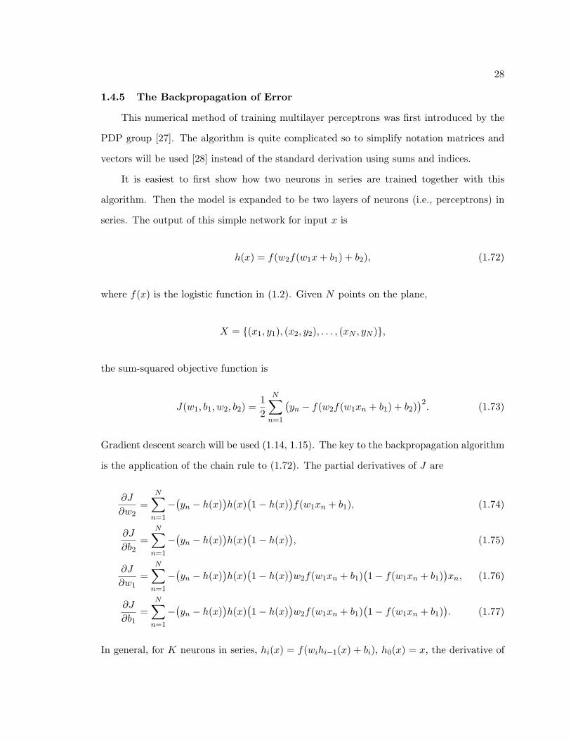
1.4.5 The Backpropagation of Error

This numerical method of training multilayer perceptrons was first introduced by the

PDP group [27]. The algorithm is quite complicated so to simplify notation matrices and

vectors will be used [28] instead of the standard derivation using sums and indices.

It is easiest to first show how two neurons in series are trained together with this

algorithm. Then the model is expanded to be two layers of neurons (i.e., perceptrons) in

series. The output of this simple network for input x is

h(x) = f(w2f(w1x+ b1) + b2), (1.72)

where f(x) is the logistic function in (1.2). Given N points on the plane,

X = {(x1, y1), (x2, y2), . . . , (xN , yN )},

the sum-squared objective function is

J(w1, b1, w2, b2) =12

N∑n=1

(yn − f(w2f(w1xn + b1) + b2)

)2. (1.73)

Gradient descent search will be used (1.14, 1.15). The key to the backpropagation algorithm

is the application of the chain rule to (1.72). The partial derivatives of J are

∂J

∂w2=

N∑n=1

−(yn − h(x)

)h(x)

(1− h(x)

)f(w1xn + b1), (1.74)

∂J

∂b2=

N∑n=1

−(yn − h(x)

)h(x)

(1− h(x)

), (1.75)

∂J

∂w1=

N∑n=1

−(yn − h(x)

)h(x)

(1− h(x)

)w2f(w1xn + b1)

(1− f(w1xn + b1)

)xn, (1.76)

∂J

∂b1=

N∑n=1

−(yn − h(x)

)h(x)

(1− h(x)

)w2f(w1xn + b1)

(1− f(w1xn + b1)

). (1.77)

In general, for K neurons in series, hi(x) = f(wihi−1(x) + bi), h0(x) = x, the derivative of

29

weight wi is the product of the derivative of each neuron and its weights for j > i and the

derivative of neuron i multiplied with the output of neuron i− 1. That product would then

be

∂J

∂wi=

N∑n=1

−(yn − h(x)

) K∏j=i+1

[hj(x)

(1− hj(x)

)wj

]hi(xn)

(1− hi(xn)

)hi−1(xn). (1.78)

For the case of an arbitrary number of inputs, outputs, and hidden nodes, matrices are

used in place of the single weights. The order of operations must be changed, too. Thus,

in the general case the backpropagation of the error is

∂J

∂Wi=

N∑n=1

−[F′i(Wizn + bi)]T

K∏j=i+1

WTj [F′

j(Wjzn + bj)]TenzTn , (1.79)

where

en = yn − FK(WKzn + bK),

and

zn = Fi−1(Wi−1 · · ·F1(W1xn + b1) + bi−1).

The dots represent the outputs of the lower layers being fed into the higher layers as inputs.

The important thing to remember about backpropagation is that the gradient for any

layer is the outer product of the output error vector and the input to the layer. This rank

1 matrix is multiplied on the left by the Jacobian matrix of the output layer activation

map, then the output layer weight matrix, then the Jacobian matrix of the highest hidden

layer’s activation map and then its weight matrix and so on until the Jacobian matrix of

the activation map of the current layer is reached.

1.5 Radial Basis Function Networks

Radial basis function networks [29] are double-layer perceptrons in which the output

layer has a linear activation function and the hidden units are Gaussian functions. If there

30

are m hidden nodes, then the output of the network from input x is

ρ(x) =m∑

i=1

wi exp(−β‖x− ci‖2). (1.80)

The vectors {c1, c2, . . . , cm} are the centroids of the network. The parameter β is a shape

parameter usually set a priori to scale the outputs of the Gaussian functions. A radial basis

function network is said to be normalized when

ρ(x) =∑m

i=1wi exp(−β‖x− ci‖2)∑mi=1 exp(−β‖x− ci‖2)

. (1.81)

Radial basis function networks are similar to Gaussian mixture models. However, there is

no requirement that each basis function be a Gaussian probability density function or that

the network compute a probability density function.

1.5.1 An Example Radial Basis Function Network

A radial basis function network used as a classifier for the example problem in sec. 1.3.3

would have c1 = (1.5, 0.5), c2 = (0.5,−0.5), β = 50, w1 = 1, and w2 = −1. This network

would have the same decision boundary as the neuron. However, it would be less confident

about its answers when x is far away from either c1 or c2. The neuron only measures the

distance of x from the decision boundary hyperplane. The radial basis functions measure

the distance of x from each of the m centroids. The shape parameter β was calculated from

the variance of the example’s data source. The variance is σ2 = 0.01. Then β = 12σ2 = 50.

1.5.2 Training a Radial Basis Function Network

The most rudimentary algorithm for training a radial basis function simply uses each

of the training input patterns {x1,x2, . . . ,xn} as the center of a radial basis function.

Thus, a training set with n patterns will generate a network with n hidden nodes using

this method. To determine the n output weights, solve the linear system: Gw = y where

31

gij = exp(−β‖xi − xj‖2). In more detail, this linear system is

1 exp(−β‖x1 − x2‖2) · · · exp(−β‖x1 − xn‖2)

exp(−β‖x2 − x1‖2) 1 · · · exp(−β‖x2 − xn‖2)...

.... . .

...

exp(−β‖xn − x1‖2) exp(−β‖xn − x2‖2) · · · 1

w1

w2

...

wn

=

y1

y2

...

yn

.

(1.82)

For large data sets this method is impractical. In such a case it is better to use a

clustering algorithm like k-means [30]. Randomly select m vectors from the training set

inputs {x1,x2, . . . ,xn} as the initial centroids {c1, c2, . . . , cm}. For each training vector

xi find the closest centroid cj to it. Add all the training vectors together that are closest

to centroid cj . Divide this vector-sum by the number of matched vectors to calculate the

new centroid. Follow this procedure once or twice again to refine the centroids. The linear

system is now overdetermined with gij = exp(−β‖xi − cj‖2). Use the pseudo-inverse of G

to find the weights.

In a classification problem with prelabeled training vectors, a centroid is calculated for

each class. For more than two classes a separate weight vector will be necessary for each

class. The output training vectors’ components will be either one or zero. If the training

vector is in the class associated with the weight vector then the component should be one;

otherwise it is zero.

For example, Fisher’s iris data set [31,32] has three classes: Iris setosa, Iris versicolor,

and Iris virginica. They are labelled 1, 2, and 3, respectively, and the training examples

are partitioned into three sets X1, X2, and X3. The three weight vectors would each be a

column in a matrix that is multiplied on the left by G. The classifications would appear in

the three columns of the matrix Y. The matrix Y would be defined as

yij =

1 xi ∈ Xj , j ∈ 1, 2, 3

0 otherwise.(1.83)

The weight matrix W would be the solution to the generalized linear system GW = Y.

32

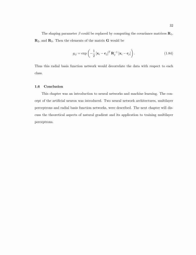
The shaping parameter β could be replaced by computing the covariance matrices R1,

R2, and R3. Then the elements of the matrix G would be

gij = exp(−1

2[xi − cj ]

T R−1j [xi − cj ]

). (1.84)

Thus this radial basis function network would decorrelate the data with respect to each

class.

1.6 Conclusion

This chapter was an introduction to neural networks and machine learning. The con-

cept of the artificial neuron was introduced. Two neural network architectures, multilayer

perceptrons and radial basis function networks, were described. The next chapter will dis-

cuss the theoretical aspects of natural gradient and its application to training multilayer

perceptrons.

33

Chapter 2

Simplified Natural Gradient

This chapter explains the theoretical development of the Simplified Natural Gradient.

The theoretical innovation is retaining the algebraic structure of the neural network pa-

rameters. These parameters are matrices. Their fundamental action is transforming the

input vectors to output vectors between two layers of nodes. It is a common practice to

reform these matrix parameters as vectors to facilitate the use of advanced optimization al-

gorithms. However, keeping the structure leads to a simplification of the Adaptive Natural

Gradient [33–35].

The Simplified Natural Gradient also uses a regularization technique [12] to prevent its

weight matrices from becoming too large as described in sec. 1.3.6. It also uses an annealed

learning rate [16] as described in sec. 1.3.8. Before these innovations and their results are

discussed in detail, the natural gradient needs to be properly introduced.

2.1 Natural Gradient

A natural gradient algorithm is an algorithm that performs the optimization of a pa-

rameter in a Riemannian (i.e., not Euclidean) space. In a Euclidean space the shortest

distance between two points is a straight line. However, in a Riemannian space the shortest

distance between two points is a curve.

Imagine the sphere with unit radius as a two-dimensional manifold S2. It is the set of

all points in R3 with unit distance from the origin. Each point on the sphere can be given

coordinates with two angles, θ and φ. The Euclidean distance between any two points

on the sphere, x1 and x2, is the measure of a line segment between the two points in R3.

However, only the endpoints of this line segment are part of the sphere S2. When measuring

their distance on the sphere, then the line segment is actually an arc on the sphere. Such

34

an arc is called a geodesic.

Looking at a typical map of the Earth such as the one drawn by Gerardus Mercator in

1569 (see fig. 2.1), it would seem that the shortest distance between two points on that map

would be along a straight line between them. However, it is not. All geodesics on a sphere

are arcs along a great circle. A great circle on S2 is a circle of radius r with its center at the

origin. Hence, the equator and the meridians on the globe are great circles. However, the

lines of latitude are small circles whose radii are less than r. This is why airline routes veer

to the north in the Northern Hemisphere and veer to the south in the Southern Hemisphere;

these routes follow great circles.

The goal of a natural gradient algorithm is to follow the curvature of the manifold

to find the best solution of a parameter by measuring the direction of steepest descent

according to the Riemannian geometry of the parameter space. This direction of descent is

natural in the sense that the algorithm follows the natural flow of the geometry.

These geometries typically come about when a parameter is constrained in some way.

For example, the two-dimensional sphere S2 is the set of all vectors {x : ‖x‖ = 1}. Con-

straining a parameter to the unit sphere is easily handled by using Lagrange multipliers

when solving an optimization in closed form. However, for more complex problems, more

sophistication may be required.

2.1.1 A Probabilistic Model

All machine learning algorithms have to deal with uncertainty. There are numerous

variations in nature. There is usually some degree of error in most measurements. Some-

times classification may be mislabelled. Regardless of the source or the reason, machine

learning algorithms compute statistics about the training data and use that information to

determine the optimal parameters for the given problem.

Suppose there is a learning model that is a parameterized function, F : Rn×Rm → Rk,

where the first argument is the parameter w of the function and the second is an input

x to be learned from training data. Let X be a random training vector with an unknown

35

Fig. 2.1: The map of the Earth drawn by Gerardus Mercator in 1569.

density function, pX(x). Let Y = F(w,X)+ζ, be a random target vector where ζ ∼ N (0, I)

represents a possible error in the training set. One possible model is

p(y1,y2, . . . ,yN |w,x1,x2, . . . ,xN ) = (2π)−Nk2 exp

(−1

2

N∑i=1

‖yi − F(w,xi)‖2

), (2.1)

where N is the number of training patterns, x1,x2, . . . ,xN are N samples of X and

y1,y2, . . . ,yN are N samples of Y. The errors ζi are not directly observable. The util-

ity of this model is derived from the fact that it is a Gaussian distribution that is also the

exponent of the neural network objective function.1

2.1.2 Sufficient Statistics

A sufficient statistic is a function of samples from a random variable with a probability

distribution with an underlying parameter such that another statistic from the same samples

does not reveal further information about the underlying parameter [37]. Formally, this1“Essentially, all models are wrong, but some are useful.” [36]

36

means that the probability distribution with the parameter is statistically independent of

the probability distribution given the sufficient statistic [38]. Given a sample x of a random

variable X, let T (x) be a statistic derived from that sample. Then T (x) is sufficient for θ

if P (X = x|T (x) = t, θ) = P (X = x|T (x) = t).

There is a way to determine if a statistic is sufficient without proving the previous

probability identity. The Fisher-Neyman factorization theorem states that a statistic T (x)

is sufficient if and only if there are functions c and a such that

fX|Θ(x|θ) = c(x)a(T (x), θ). (2.2)

If the probability density function ofX given the parameter θ can be factored into a function

of the sample(s) times a function of the parameter and the statistic, then the statistic is

sufficient.

For example, let X be a random variable that maps to the set {0, 1} with a Bernoulli

distribution with parameter 0 < p < 1. Given a sequence of samples x1, x2, . . . , xN of X,

the joint probability mass function of these samples is

fX(x1, x2, . . . , xN |p) = px1(1− p)1−x1px2(1− p)1−x2 · · · pxN (1− p)1−xN

= px1+x2+···+xN (1− p)N−(x1+x2+···xN ). (2.3)

Let T (x1, x2, . . . , xN ) = x1 + x2 + · · ·+ xN , then

fX(x1, x2, . . . , xN |p) = pT (x1,x2,...,xN )(1− p)N−T (x1,x2,...,xN ). (2.4)

By choosing c(x) = 1 and a(t, p) = pt(1− p)N−t, the probability mass function of X can be

factored. Thus, T (x) is sufficient for p.

37

2.1.3 The Exponential Family

There is a special family of probability distributions called the exponential family. Each

distribution in the family has a PDF that can be factored as

fX|Θ(x|θ) = c(x) exp(η(θ)T (x)−A(θ)). (2.5)

Hence, it is relatively straightforward to find a sufficient statistic for a parameter if the

underlying distribution is a member of the exponential family. For example, the Bernoulli

distribution with parameter p is a member of the exponential family. Choose c(x) = 1 and

a(T (x1, x2, · · · , xN ), p) = exp((log p− log(1− p))T (x1, x2, . . . , xN ) +N log(1− p)). (2.6)

Thus, η(p) = log p− log(1− p) and A(p) = −N log(1− p).

There are exponential families for random vectors whose distributions have multiple

parameters. There are also multiple statistics. Their general form is

fX|Θ(x|θ1, θ2, . . . , θd) = c(x) exp

(r∑

i=1

ηi(θ1, θ2, . . . , θd)Ti(x)−A(θ1, θ2, . . . , θd)

). (2.7)

2.1.4 Optimal Parameter Estimation

If the goal is to find the optimal parameter, θ, then the log-likelihood function provides

a mechanism through which the parameters can be estimated in terms of the sufficient

statistic. The log-likelihood function is the natural logarithm of the probability density

function

`(x, θ) = log(fX|Θ(x|θ))

= log(c(x)) + η(θ)T (x)−A(θ).(2.8)

To find the optimal parameter, take the derivative of the log-likelihood function

∂`

∂θ=∂η

∂θT (x)− ∂A

∂θ. (2.9)

38

This is called the score function. Like many other optimization problem, the optimal pa-

rameter is the one for which the derivative of the function vanishes. In estimation problems,

the derivative is the score function, so the best parameter has a score of zero. For example,

the score function of the Bernoulli distribution is

∂`

∂p=T (x1, x2, . . . , xN )

p(1− p)− N

1− p= 0. (2.10)

Solving for p gives the optimal parameter estimate, p = 1N T (x1, x2, . . . , xN ) = 1

N

∑Ni=1 xi.

This is the maximum likelihood (ML) estimate of p. The score function of the PDF in (2.1)

is the vector-valued function

∂`

∂w=

N∑i=1

(∂F∂w

)T

(yi − F(w,xi)), (2.11)

where ∂F∂w =

[∂fi

∂wj

]is the Jacobian matrix of F. The optimal parameter cannot be found

directly by solving (2.11). A gradient descent algorithm is commonly used.

2.1.5 The Fisher Information

The performance of a gradient descent algorithm may be improved significantly by

using Newton’s method [22]. Newton’s method divides the first derivative of the function

by its second derivative. The score function of a random variable from a distribution with

a single parameter is∂`

∂θ=

1fX|Θ(x|θ)

∂fX|Θ

∂θ. (2.12)

Hence, the second derivative is

∂2`

∂θ2= − 1(

fX|Θ(x|θ))2 [∂fX|Θ

∂θ

]2

+1

fX|Θ(x|θ)∂2fX|Θ

∂θ2. (2.13)

For a log-likelihood function with multiple parameters, its gradient vector is multiplied by

the inverse of its Hessian matrix. This works well for points in the parameter space close to

a minimum. However, when one or more of the eigenvalues of the Hessian matrix approach

39

zero, then Newton’s method will fail because of division by a number close to zero.

With maximum likelihood estimation, the Fisher information G(θ) is used instead of

the Hessian matrix. It is the expected value of the second derivative of the log-likelihood

function

G(θ) = E

{∂2`

∂θ2

∣∣∣∣θ} = −∫ ∞

−∞

[∂`

∂θ

]2

fX|Θ(x|θ)dx+∫ ∞

−∞

∂2fX|Θ

∂θ2dx. (2.14)

When the second term of (2.14) is required to be zero as a regularity constraint, then the

formal definition of the Fisher information is

G(θ) = E

{[∂`

∂θ

]2 ∣∣∣∣θ}. (2.15)

Since the mean of the score is zero, it is also the variance of the score [39,40]. For example,

the Fisher information of the Bernoulli distribution with parameter p is

G(p) = −E{∂2`

∂p2

∣∣∣∣p}= E

{(1− 2p)T (x1, x2, . . . , xN )

p2(1− p)2

∣∣∣∣p}+N

(1− p)2

=Np(1− 2p)p2(1− p)2

+N

(1− p)2

=N

p(1− p). (2.16)

Dividing the score function of the Bernoulli distribution by the Fisher information simplifies

the terms1

G(p)∂`

∂p=

1NT (x1, x2, . . . , xn)− p = 0. (2.17)

When the parameter is a vector, then the Fisher information is a matrix. The matrix

is the expected value of the outer product of the score function with itself

G(θ1, θ2, . . . , θd) = E{∇θ`(∇θ`)T |θ1, θ2, . . . , θd

}. (2.18)

40

Except for a few pathological cases, the Fisher information matrix is positive definite.

2.1.6 The Geometry of Exponential Families

For an exponential family there is an affine geometry on its parameters [41, 42]. The

points in this geometry are probability measures. For each point p in the set of all probability

measures P there is a tangent space TpP . The tangent vectors are the random variables

defined with the probability measure p. Random variables are functions that map events

to the real numbers. If the event space is defined as the real numbers, then the random

variables will also transform one probability measure into another. The action of a random

variable X on a probability measure p is p + X = exp(X)p. The action follows the rules

of addition. If Y is another random variable, then (p + X) + Y = exp(Y ) exp(X)p =

exp(Y +X)p = p+ (X + Y ).

A coordinate system can be chosen for this affine geometry. These coordinates are

the parameters for the probability measures in P . Suppose that the vector components

(θ1, . . . , θr) are the coordinates for a probability measure p, then there are r random vari-

ables X1, . . . , Xr that are sufficient statistics for θ1, . . . , θr. Since P is an exponential family,

p = exp(θ1X1 + · · ·+ θrXr −K). (2.19)

Coordinates such as these are the canonical coordinates. Any coordinate system can be

transformed into a canonical coordinate system by selecting the appropriate functions.

There is a log-likelihood function `(p) associated with each probability measure p in

P . It is the natural logarithm of p

`(p) = θ1X1 + · · ·+ θrXr −K. (2.20)

Furthermore, the score functions are

∂`

∂θi= Xi. (2.21)

41

Thus, the score functions form a basis for the tangent space TpP . An inner product can be

defined on TpP . For two random variables Y and Z, the inner product is defined as

〈Y, Z〉 = Ep[Y Z], (2.22)

where Ep is the expectation operator using the probability measure p. The elements of the

Fisher information matrix are

gij = Ep[XiXj ] = 〈Xi, Xj〉. (2.23)

The matrix of the inner products of the basis vectors of a tangent space is also the Rieman-

nian metric for a metric space. Thus, for an exponential family used as a metric space, the

metric is the Fisher information matrix.

2.1.7 Direction of Steepest Descent

Given a function f : Rn → R, its gradient ∇f is the direction of positive increase or

ascent of the function f in Rn. Clearly, −∇f would be the direction of descent. Thus,

any vector v ∈ Rn, is a descent direction if 〈v,∇f〉 < 0. Let h(v) = 〈v,∇f〉 be a linear

functional. Clearly, h(v) reaches its minimum when v = −∇f since h(−∇f) = −‖∇f‖2.

For any probability measure p, the gradient of its log-likelihood function is likewise

a tangent vector. Thus, the gradient ∇(log p) =∑r

i=1 σiXi where σi is the score of p on

parameter i. Similarly, a random variable V is a descent direction if 〈V,∇(log p)〉 < 0.

Thus, if V =∑r

i=1 τiXi, then the inner product is

〈V,∇(log p)〉 =r∑

i=1

r∑j=1

gijσiτ j . (2.24)

The steepest descent direction will always be

V = −G−1∇(log p), (2.25)

42

where G is the Fisher information matrix.

2.2 Amari’s Adaptive Natural Gradient for Multilayer Perceptrons

The Adaptive Natural Gradient Learning (ANGL) algorithm for multilayer percep-

trons [34, 35] is a Newton-type algorithm that uses the Fisher information matrix instead

of the Hessian matrix. It is an online learning algorithm that performs an autoregressive

estimate of the Fisher information matrix with a learning rate εt

Gt+1 = (1−εt)Gt+εt

(∂F(w,xi)

∂w

)T

(yi−F(w,xi))(yi−F(w,xi))T

(∂F(w,xi)

∂w

). (2.26)

Instead of inverting the Fisher information after each pattern, the inverse is updated as a

rank-1 update using the matrix inversion lemma [40]

G−1t+1 = (1 + εt)G−1

t − εtG−1

t

(∂F(w,xi)

∂w

)T(yi − F(w,xi))(yi − F(w,xi))T

(∂F(w,xi)

∂w

)G−1

t

1 + (yi − F(w,xi))T(

∂F(w,xi)∂w

)G−1

t

(∂F(w,xi)

∂w

)T(yi − F(w,xi))

.

(2.27)

Amari shows that the best adaptation rate is εt = 1t . It must be noted that the Adap-

tive Natural Gradient Learning algorithm uses the common convention of ordering all the

parameters into one large vector. Let the homomorphism φ denote this operation on the

parameters of a multilayer perceptron. Then for the parameters, W1, b1, etc., there is a

vector w such that

φ(W1,b1,W2,b2, . . . ) = w. (2.28)

Typically, the columns of each matrix are stacked on top of each other with the bias vectors

interleaved between the matrices. Regardless, this has the effect of making the Fisher

information matrix very large. However, maintaining this structure may yield other benefits.

2.3 Algebraic Structure of Multilayer Perceptrons

As was discussed in sec. 1.4.5, each layer of a multilayer perceptron is an affine trans-

formation with a transfer function that restricts the output of each layer to either the

43

interval [0, 1] or the interval [−1, 1]. Understanding how the derivatives work is necessary

to developing any kind of gradient descent algorithm. Let W be the weight matrix for a

single-layer perceptron with b as its bias and F as its transfer function. Let x and y be

a generic input-output pair from a suitable training set. The squared error of this pair is

J(W,b) = 12‖y − F(Wx + b)‖2.

2.3.1 Directional Derivative

This section describes in detail how the derivatives of the function J are computed.

This will lead into developing the Fisher information matrix and the natural gradient of a

multilayer perceptron. The first step is to find the directional derivative of J in the direction

of steepest descent.

Given a weight matrix W and a bias vector b, assume that the matrix V and the

vector c are the steepest descent direction from (W,b) toward the optimal solution. Let

γ(t) = W + tV be the line through the space of possible weight matrices and θ(t) = b + tc

be the line through the space of possible bias vectors that follows the steepest descent

direction. Then their derivatives are γ(t) = V and θ(t) = c. By composing J with the

tuple (γ(t), θ(t)) the real-valued function of the single parameter, t, is defined, J(γ(t), θ(t)).

The derivative of this function is

d

dt(J(γ(t), θ(t))) = lim

t→0

J(W + tV,b + tc)− J(W,b)t

. (2.29)

There is a problem with (2.29). The variable t cannot be directly factored out of the

expression J(W + tV,b + tc). However, since the transfer function F is differentiable, its

Jacobian matrix can be used in a first-order Taylor series of J . This first-order Taylor series

of J expanded about W is

J(W + tV,b) = J(W,b) +⟨∂J

∂W, tV

⟩, (2.30)

44

and the first-order Taylor series of J expanded about b is

J(W,b + tc) = J(W,b) +⟨∂J

∂b, tc⟩. (2.31)

Therefore, using (2.29), (2.30), and (2.31), the directional derivative of J in the direction

of (V, c) isdJ

dt=

d

dtJ(γ(t), θt) =

⟨∂J

∂W,V⟩

+⟨∂J

∂b, c⟩. (2.32)

The next step is to find the partial derivatives ∂J∂W and ∂J

∂b . If t, V and c can be

isolated, then t will vanish in the limit, the matrix in the inner product with V will be ∂J∂W

and the vector in the inner product with c will be ∂J∂b . This is accomplished by using the

first-order Taylor series of F. Expanding F about W is

F((W + tV)x + b) = F(Wx + b) + tF′(Wx + b)Vx, (2.33)

where F′(z) =[

∂fi

∂zj

]is the Jacobian matrix of F. Similarly, the first-order Taylor series

expansion of F about b is

F(Wx + b + tc) = F(Wx + b) + tF′(Wx + b)c. (2.34)

The composition of the objective function J with the curve γ(t) is

J(γ(t),b) = J(W + tV,b) =12‖y − F((W + tV)x + b)‖2. (2.35)

45

The partial derivative with respect to W can be found by differentiating with respect to t.

Thus, the derivative is

d

dtJ(W + tV,b) = −

⟨y,

d

dtF((W + tV)x + b)

⟩+

12d

dt‖F((W + tV)x + b)‖2

= −⟨y,F′(Wx + b)Vx

⟩+⟨F(Wx + b),F′(Wx + b)Vx

⟩= −

⟨Vx,F′(Wx + b)T (y − F(Wx + b))

⟩= −xTVTF′(Wx + b)T (y − F(Wx + b))

= − tr(VTF′(Wx + b)T (y − F(Wx + b))xT

)= −

⟨V,F′(Wx + b)T (y − F(Wx + b))xT

⟩,

(2.36)

where the last inner product in (2.36) is the Matrix Inner Product (i.e., 〈A,B〉 = tr(ATB)).

Similarly, the composition of J with θ(t) is

J(W, θ(t)) = J(W,b + tc) =12‖y − F(Wx + b + tc)‖2. (2.37)

It’s derivative with respect to t is

d

dtJ(W,b + tc) = −

⟨y,

d

dtF(Wx + b + tc)

⟩+

12d

dt‖F(Wx + b + tc)‖2

= −⟨y,F′(Wx + b)c

⟩+⟨F(Wx + b),F′(Wx + b)c

⟩= −

⟨c,F′(Wx + b)T (y − F(Wx + b))

⟩.

(2.38)

Therefore, the partial derivatives with repect to the weight matrix W and the bias

vector b are

∂J

∂W= −F′(Wx + b)T (y − F(Wx + b))xT , (2.39)

∂J

∂b= −F′(Wx + b)T (y − F(Wx + b)). (2.40)

Please note that the dimensions of both partial derivatives are those of the parameters W

and b, respectively. Typically, in almost all neural network training algorithms, all the

46

parameters are stacked into one large vector. However, these parameters are used as affine

transformations. Therefore, their algebraic structure is preserved.

2.3.2 The Fisher Information Matrix of a Single-Layer Perceptron

Let e = y − F(Wx + b) be the N (0, I) random variable that is the error of the

perceptron for x and y. The Fisher information matrix using this model is then

G(W,b) = E

{∇J(∇J)T

∣∣∣∣W,b,x}

= E

{[∂J

∂W∂J

∂b

] [∂J

∂W∂J

∂b

]T ∣∣∣∣W,b,x

}

= E

{∂J

∂W

(∂J

∂W

)T

+∂J

∂b

(∂J

∂b

)T ∣∣∣∣W,b,x

}

= E

{F′(Wx + b)TexT

(F′(Wx + b)TexT

)T ∣∣∣∣W,b,x}

+ E

{F′(Wx + b)Te

(F′(Wx + b)Te

)T ∣∣∣∣W,b,x}

=(xTx + 1

)F′(Wx + b)TE

{eeT

∣∣W,b,x}F′(Wx + b)

=(xTx + 1

)F′(Wx + b)TF′(Wx + b).

(2.41)

This version of the Fisher information matrix is more compact than that used in (2.26). The

gradient used in the ANGL is a vector with a component for every weight matrix element

and bias vector component. The outer product of that gradient with itself is a large, rank-1

matrix. In contrast, the gradient computed in (2.39) is the same size as W and in (2.40)

the gradient has the same dimension as b. Therefore, the Fisher information matrix in

(2.41) is square with the number of rows and number of columns both equal to the number

of outputs of the neural network. Now the gradient of J is

∇WJ = −(F′(Wx + b)TF′(Wx + b)

)−1 F′(Wx + b)TexT

xTx + 1, (2.42)

∇bJ = −(F′(Wx + b)TF′(Wx + b)

)−1 F′(Wx + b)TexTx + 1

. (2.43)

Hence, in this example, the natural gradient is the product the pseudo-inverse of the

47

Jacobian matrix of F and the outer product of the errors and the inputs all divided by the

squared length of the input vectors offset by one. Given that the Jacobian matrices of most

transfer functions used in neural networks are square and diagonal,2 the pseudo-inverse is

really just the inverse of a diagonal matrix.

When there is more than one training example (a very desirable situation), then the

computation of the Fisher information matrix is more complicated. For online learning,

(2.42) and (2.43) can be used on each individual training pattern. Assuming that the

Jacobian matrix is square, real-symmetric and invertible, the natural gradient simplifies to

∇WJk = −F′(Wxk + b)−1ekxT

k

xTk xk + 1

, (2.44)

∇bJk = −F′(Wxk + b)−1ek

xTk xk + 1

. (2.45)

One problem with this formulation is that as the weights become saturated, the Jacobian

matrix becomes nearly-singular. Even more problematic is its implicit reliance on the

accuracy of the model.

A more robust approach starts from the objective function,

J(W,b) =12

N∑i=1

‖yi − F(Wxi + b)‖2, (2.46)

that measures the sum-squared error. Using the derivatives calculated in (2.39) and (2.40),

the partial derivatives of the sum-squared error are

∂J

∂W= −

N∑i=1

F′(Wxi + b)T (yi − F(Wxi + b))xTi , (2.47)

∂J

∂b= −

N∑i=1

F′(Wxi + b)T (yi − F(Wxi + b)). (2.48)

2One exception to this is the soft-max function. Its Jacobian matrix is square and real-symmetric.

48

Let ei = yi−F(Wxi +b) be the error of training example i. The unbiased estimate of the

Fisher information matrix is

G =1

N − 1

N∑i=1

(xT

i xi + 1)F′(Wxi + b)TeieT

i F′(Wxi + b). (2.49)

This model will be able to adjust to skewed data sets and noisy data by estimating the

mean and variance of the error and using them in its estimate of the Fisher information

matrix.

2.3.3 The Fisher Information Matrix of a Multilayer Perceptron

So far, the focus has been the Fisher information matrix of a single-layer network.

This section will generalize the model to multilayer perceptrons. An L-layer feed-forward

network is functionally an alternating sequence of matrices and nonlinear transfer functions.

The output of layer l ∈ {1, 2, . . . , L} depends on its current input, the output of layer l− 1,

along with the parameters Wl and bl. These are combined into a vector that the nonlinear

transfer function, Fl, squashes. There is a recurrence relation between the outputs of

succeeding layers in the network. Let ϕ0(xn) = xn represent the inputs to the network.

Then each layer l has the output ϕl(xn) = Fl(Wlϕl−1(xn) + bl). This allows the objective

to be written simply as

J(W1, . . . ,WL,b1, . . . ,bL) =12

N∑i=1

‖yi − ϕL(xi)‖2. (2.50)

Using (2.39), (2.40), and the chain rule, the partial derivatives of the objective function

J with respect to the output layer weights, output layer bias, last hidden layer weights, and

49

last hidden layer bias, respectively, are

∂J

∂WL= −

N∑i=1

ϕ′L(xn)T (yn − ϕL(xn))ϕL−1(xn)T , (2.51)

∂J

∂bL= −

N∑i=1

ϕ′L(xn)T (yn − ϕL(xn)), (2.52)

∂J

∂WL−1= −

N∑i=1

ϕ′L−1(xn)TWTLϕ

′L(xn)T (yn − ϕL(xn))ϕL−2(xn)T , (2.53)

∂J

∂bL−1= −

N∑i=1

ϕ′L−1(xn)TWTLϕ

′L(xn)T (yn − ϕL(xn)). (2.54)

Just as the output of each layer l of the network depends not only on its own weights and

biases, but on the weights and biases of the previous layers, the backpropagation of the

error depends on the weights of successive layers. This is best expressed as a recurrent

relation as

ζL(xn) = ϕ′L(xn), (2.55)

ζL−1(xn) = ζL(xn)WLϕ′L−1(xn), (2.56)

ζl(xn) = ζl+1(xn)Wl+1ϕ′l(xn). (2.57)

The image of the map ζl is a backpropagation transformation. This will transform the

error vector such that the change in a weight matrix depends on the strength of each

connection [27]. By substituting these formulae into the equations of the partial derivatives,

the equations can be written as

∂J

∂Wl= −

N∑i=1

ζl(xn)T (yn − ϕL(xn))ϕl−1(xn)T , (2.58)

∂J

∂bl= −

N∑i=1

ζl(xn)T (yn − ϕL(xn)). (2.59)

The Fisher information matrix of a multilayer perceptron can be conceived as an L×L

block matrix with each matrix in the diagonal being the Fisher information matrix of a

50

layer’s parameters. Thus, the Fisher information matrix for the network parameters of

layer l would be

Gl =1

N − 1

N∑i=1

(ϕl−1(xi)Tϕl−1(xi) + 1

)ζl(xi)TeieT

i ζl(xi). (2.60)

Inverting this matrix involves only inverting the blocks along the main diagonal. The

learning rule for each layer would then be

Wl(t+ 1) = Wl(t) + η(t)G−1l (t)

∂J

∂Wl, (2.61)

bl(t+ 1) = bl(t) + η(t)G−1l (t)

∂J

∂bl, (2.62)

where t represents the current learning epoch. This is the Simplified Natural Gradient

learning rule.

2.4 Simplified Natural Gradient Example

This section shows how the Fisher information matrix would be calculated for the

neural network described in sec. 1.4.4. The input vectors of the XOR problem are

x0 =

−1

−1

, x1 =

−1

1

, x2 =

1

−1

, x3 =

1

1

. (2.63)

The corresponding outputs of the XOR problem are

y0 = −1, y1 = 1, y2 = 1, y3 = −1. (2.64)

The transfer functions, weight matrices and bias thresholds as determined in sec. 1.4.4 are

F1(a1) = tanh(a1), W1 =

2 −2

−2 2

, b1 =

−2

−2

, (2.65)

f2(a2) = tanh(a2), W2 =[1 1

], b2 = 1. (2.66)

51

Thus, the outputs of the hidden layer are

F1(W1x0 + b1) =

−0.9640

−0.9640

, F1(W1x1 + b1) =

−1.0000

0.9640

, (2.67)

F1(W1x3 + b1) =

−0.9640

−0.9640

, F1(W1x2 + b1) =

0.9640

−1.0000

. (2.68)

The final outputs of the two-layer perceptron are then

f2(W2F1(W1x0 + b1) + b2) = −0.7297, f2(W2F1(W1x1 + b1) + b2) = 0.7461, (2.69)

f2(W2F1(W1x3 + b1) + b2) = −0.7297, f2(W2F1(W1x2 + b1) + b2) = 0.7461. (2.70)

These outputs are used to compute the errors of each training pattern

e0 = −0.2703, e1 = 0.2539, e2 = 0.2539, e3 = −0.2703. (2.71)

The estimated variance of the error is then computed to be

E{e2}

= 0.2751. (2.72)

The partial derivatives of the objective function are then computed as

∂J

∂W1=

0.0080 −0.0080

−0.0080 0.0080

, ∂J

∂b1=

−0.0099

−0.0099

, (2.73)

∂J

∂W2=[0.2396 0.2396

],

∂J

∂b2= −0.0276. (2.74)

52

This gives the estimates of the Fisher information of each layer as

G1 =

0.2174 −0.1500

−0.1500 0.2174

× 10−3, (2.75)

g2 = 0.0550. (2.76)

The inverse of G1 is

G−11 =

8.7793 6.0575

6.0575 8.7793

× 103, (2.77)

1g2

= 18.1818. (2.78)

These are obviously large values. Using the inverse of the Fisher information matrix in the

place of the Hessian in a Newton-type algorithm has the same problems when the errors

get small: The inverse becomes large and that drives the values of the weights to become

large. This can lead to severe overtraining. However, if the same mechanism for avoiding

overtraining is used as described in sec. 1.3.6, then these effects can be mitigated.

2.5 Adding a Prior Distribution with a Hyperparameter

The prior distribution on the weight matrix of level l, Wl, has the PDF

pWl(Wl) = exp

(−1

2α‖Wl‖2

). (2.79)

The mean value of Wl is E{Wl} = 0. The variance of its norm tr(WlWTl ) is

E{tr(WlWT

l

)}=

1α. (2.80)

By using the modified partial-derivative (1.21) in the Fisher information matrix (2.60), then

the definition of the estimate of the Fisher information matrix is modified by adding αI to

it. For example, if α = 0.1, then the inverse of the modified Fisher information matrix in

53

(2.75) would be

(G1 + αI)−1 =

9.9783 0.0149

0.0149 9.9783

, (2.81)

1g2 + α

= 6.4516. (2.82)

The regularization of the gradient values carries through to the definition of the Fisher

information matrix. The modified Fisher information matrix definition is

Gl =1

N − 1

N∑i=1

(ϕl−1(xi)Tϕl−1(xi) + 1

)ζl(xi)TeieT

i ζl(xi) + αI. (2.83)

To explain this definition let Gα be the Fisher information matrix computed with the

augmented gradient as compared to the Fisher information matrix G computed with just

the gradient ∇J . Thus, the modified Fisher information matrix is computed as

Gα = E{(∇J − αW)(∇J − αW)T

},

= E{∇J(∇J)T − α

((∇J)WT + W(∇J)T

)+ α2WWT

},

= E{∇J(∇J)T

}− αE

{(∇J)WT + W(∇J)T

}+ α2E

{WWT

},

= G + αI.

(2.84)

The following question arises: Why is E{∇JWT } = 0? In the case of the neuron, it can

be shown to be zero simply by substituting z = y − f(wTx + b) and rearranging the order

54

of operations in the expectation integral

E{∇JwT } =∫f ′(wTx + b)[y − f(wTx + b)]xwT ·

exp(−1

2[y − f(wTx + b)]2 − 1

2α‖w‖2

)dy dw dx,

=∫zf ′(wTx + b)xwT exp

(−1

2[z2 + α‖w‖2

])dz dw dx

=∫ ∞

−∞z exp

(−1

2z2

)dz

∫f ′(wTx + b)xwT exp

(−1

2α‖w‖2

)dw dx,

= 0.

(2.85)

The statistical model assumes that y = f(wTx + b) + z for any x, y or w. The random

variable z is normally distributed, z ∼ N (0, 1). Hence, Ez = 0. It is also assumed that

z is independent of x and w. This may seem to be an incorrect assumption at first as z

is computed from y, x, and w. However, the network is correlating the input x with y by

changing w. That implies that z would be decorrelated. These are really only mathematical

arguments to justify an algorithm design decision based on empirical results. These cross

terms are very small and do not significantly impact the performance of the algorithm. Just

as the cross terms of the neuron’s Fisher information matrix are determined to be zero, so

are the cross terms of the multilayer perceptron’s Fisher information matrix.

2.6 Conclusion

Natural gradient is a gradient-descent technique that uses the Fisher information matrix

of the parameter estimator as the Riemannian metric of a manifold. With neural networks,

this allows a learning algorithm to follow the manifold to find better parameters to solve

problems.

This chapter has described the Simplified Natural Gradient Learning Algorithm and

its differences with ordinary gradient descent and Amari’s Adaptive Natural Gradient. The

next chapter will discuss the empirical results from experiments carried out to compare

these algorithms.

55

Chapter 3

Experimental Results

The following experiments compare the performance of the Ordinary Gradient Learning

(OGL) algorithm, the Adaptive Natural Gradient Learning (ANGL) algorithm, and the

Simplified Natural Graident Learning (SNGL) algorithm described in this thesis for training

multilayer perceptrons (MLPs).

The first experiment teaches a network to learn the XOR (eXclusive OR) function. It

is not linearly separable and the properties of its parameter space (as an MLP learning

this function) have been studied in depth [14, 26, 35, 43]. Remember that a simple neuron

can only learn linearly separable functions. This is because a neuron finds the hyperplane

with which to divide its inputs. If a problem is not linearly separable, then a multilayer

perceptron must be used. XOR is an excellent example because there are four points on

the plane for which there is no line that can separate them according to their labeling.

The second experiment teaches a network to encode a 5-bit message using a Low-

Density Parity Check (LDPC) code. The encoding function adds 5 parity check bits to the

message bits. It is similar to XOR but has a much larger parameter space.

The next experiment teaches a network to recognize three different species of Iris: Iris

setosa, Iris versicolor, and Iris virginica. The experiment uses Fisher’s Iris data [31].

The Mackey-Glass chaotic time series prediction problem tests a neural network train-

ing algorithm’s ability to predict data. If x(t) is the Mackey-Glass series for the index t,

then the problem is to predict x(t+ 6) given x(t), x(t− 6), x(t− 12), and x(t− 18).

Finally, Nonlinear Dimension Reduction will be used to generate interesting data sets

to train an MLP to compute a nonlinear dimension-reducing map. Nonlinear Dimension

Reduction algorithms transform data embedded on a curved surface in a higher-dimensional

manifold. The algorithms work on finite sets by maximizing the distance between distant

56

points while holding the distance between close points to be constant. This unfolds the

surface onto a lower-dimensional Euclidean space. However, the algorithm does not produce

the map from the surface to the Euclidean space. This is an excellent problem for a Machine

Learning algorithm because sufficient data available for both training and testing.

3.1 Effective Learning Rate

Neural network training algorithms are very sensitive to the learning rate. In the OGL

algorithm, the step-size for each learning epoch is η‖∇J‖. The natural gradient algorithms

have a step-size of η‖G−1∇J‖. An interesting point of comparison is the relative step-sizes

of these algorithms. Since the Fisher information matrix is positive-definite in most cases,

then all its eigenvalues are positive. Therefore, if λ is the largest eigenvalue of G−1, then

λ‖∇J‖ ≥ ‖G−1∇J‖. For the Simplified Natural Gradient Learning algorithm, the largest

eigenvalue of G−1 is the multiplicative inverse of the smallest eigenvalue of G. Thus, for

SNGL, the effective learning rate is ηλ1

where λ1 is the smallest eigenvalue of G. For ANGL,

the effective learning rate is the product of the nominal learning rate η and the largest

eigenvalue of the estimate of G−1.

3.2 Exclusive OR Problem (XOR)

The XOR Problem was used as an example in secs. 1.4.4 and 2.4. In review, the

network is to be trained to compute the XOR function. Again, this function is not linearly

separable (see fig. 3.1). The inputs and outputs are

x0 =

−1

−1

, x1 =

−1

1

, x2 =

1

−1

, x3 =

1

1

, (3.1)

y0 = −1, y1 = 1, y2 = 1, y3 = −1, (3.2)

respectively. The architecture is a two-layer perceptron with hyperbolic tangent transfer

functions between both the hidden units and the output units. Thus, the error for each

57

pattern is

εn = yn − tanh (W2 tanh (W1xn + b1) + b2) . (3.3)

There are two hidden units and each layer has a bias. Hence, W1 is a 2-by-2 matrix and

W2 is a 1-by-2 matrix. The bias vector b1 is a 2-vector and b2 is a scalar. The source code

for these experiments is in appendix A.

The first part of this experiment is to inspect the eigenvalues of the Fisher information

matrix. Next, a performance comparison will be measured between the three algorithms

OGL, SNGL, and ANGL using the sum-squared error metric:

J(W1,W2,b1, b2) =12

3∑n=0

(yn − tanh (W2 tanh (W1xn + b1) + b2))2 . (3.4)

Finally, the effective learning rate of each algorithm will be investigated.

3.2.1 The Eigenvalues of the Fisher Information Matrix

Figure 3.2 shows the eigenvalues of the Fisher information matrix for each learning

epoch of the SNGL algorithm. For this algorithm the effective learning rate is its learning

rate divided by the largest eigenvalue of the Fisher information matrix. The eigenvalues

λ1 and λ2 belong to the 2-by-2 Fisher information matrix of the first layer of connection

weights and λ3 is actually just the scalar value g2 because the Fisher information matrix of

the second layer is a 1-by-1 matrix.

These eigenvalues only have significant values during the first ten learning epochs. In

later epochs, the Fisher information matrix is very close to αI because the gradient matrices

are so small.

3.2.2 Performance Comparison

Figure 3.3 shows the sum-squared error computed by (3.4) of each learning epoch for

OGL, SNGL, and ANGL. Note that the epochs in which the biggest improvements are

achieved by the SNGL algorithm are the first ten for which the eigenvalues of the Fisher

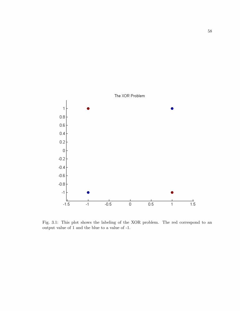
58

Fig. 3.1: This plot shows the labeling of the XOR problem. The red correspond to anoutput value of 1 and the blue to a value of -1.

59

Fig. 3.2: This plot shows the eigenvalues of the Fisher information matrix for each learningepoch. The Fisher information is a metric for the variance of the parameters around thecurrent estimate. High variance means that there more information to be gleaned from thedata into the parameters.

60

information matrix are significant in fig. 3.2. Both the OGL and ANGL algorithms were

stuck in plateaus for the first two hundred learning epochs.

Table 3.1 shows the parameters used in the three learning algorithms and some of the

results of the experiment. The nominal learning rate is the actual step size η chosen in the

learning rules of the learning algorithms. The initial learning rate is the effective learning

rate used in the first learning epoch.

The learning rate is annealed in the SNGL algorithm as described in sec. 1.3.8. This

is done to counteract the learning rate approaching ηα when the Fisher information matrix

gets close to αI in the later learning epochs. The OGL algorithm’s performance did not

improve when using an annealed learning rate.

In the ANGL algorithm, a fixed learning rate is used. However, the adaptation rate

used in the autoregressive estimator of the inverse of the Fisher information matrix given

in (2.27) is chosen to be 1t in [34, 35]. In the implementation used in this experiment, the

adaptation rate is chosen to be min(0.1, 1

t

)so that the algorithm actually converges.

Equations (3.5-3.10) show the final values of the parameters computed by the algo-

rithms. The ANGL algorithm computes slightly larger parameters because including the

prior distribution on the weights causes the Fisher information matrix to approach infinity

and fail. As the algorithm continues to run the absolute values of the parameters increase

without bound. However, the ratio between any two parameters is relatively constant.

Thus, it is overtraining in the later epochs. The final values of the parameters in the OGL

algorithm are

W1 =

1.7280 1.7280

1.7280 1.7280

, b1 =

−1.6535

1.6535

, (3.5)

W2 =[−1.7377 1.7377

], b2 = −1.5822. (3.6)

61

Fig. 3.3: The sum-squared error curves of OGL, ANGL, and SNGL with effective learningrate η = 0.25 and SNGL modified to use an annealed learning rate.

Table 3.1: The results of and parameters used for the OGL, SNGL, and ANGL algorithmson the XOR problem.

XOR OGL SNGL ANGL

Hidden Units 2 2 2Nominal Learning Rate 0.25 0.25 0.01Initial Learning Rate 0.25 6.5351 0.2574Annealed Learning Rate Yes Yes NoPrior Probability on Parameters Yes Yes NoHyperparameter of Prior Distribution 0.01 0.01 N/AFisher Information Matrix Size N/A (1, 2) 9Adaptation Rate N/A N/A min

(0.1, 1

t

)Number of Extra Parameters 0 5 81Final Learning Rate 1e-4 0.0097 0.1157Final Sum-Squared Error 0.0902 0.0289 3.6627e-4Learning Epoch when SSE < 0.0289 10,000 11 127

62

The final values of the parameters in the SNGL algorithm are

W1 =

1.7280 −1.7280

−1.7280 1.7280

, b1 =

−1.6536

−1.6536

, (3.7)

W2 =[1.7377 1.7377

], b2 = 1.5822. (3.8)

The final values of the parameters in the ANGL algorithm are

W1 =

−2.9141 −2.9142

−2.9108 −2.9107

, b1 =

−2.8228

2.8251

, (3.9)

W2 =[2.7112 −2.7116

], b2 = −2.6101. (3.10)

One interesting side note is worth discussing. Because the hyperbolic tangent function

is an odd function, negating column i in W2 and negating row i in W1 and element i in

b1 does not change the function that the network computes. Furthermore, permuting the

columns of W2 and applying the same permutation to the rows of W1 and the elements of

b1 also does not change the function that the network computes. Therefore, the parameters

in eqs. (3.5-3.8) are equivalent.

Figure 3.4 shows the effective learning rates for all three algorithms. It shows some

interesting behavior of the SNGL algorithm. The SNGL algorithm takes one large step in

the first epoch followed by several small steps. Then it takes a few more big steps and then

it slowly backs off as the effects of the prior distribution hold it back from overtraining.

Essentially, SNGL has a variable learning rate for each layer in the network. This is where

the real power of the Simplified Natural Gradient Learning algorithm comes into play. The

steps taken are governed by the Fisher information of the parameters in each layer. The

ANGL algorithm also performs very well. Again, the prior distribution is not used in the

ANGL algorithm because it causes instability in the estimate of the Fisher information

matrix’s inverse. Note that its effective learning rate increases in later epochs.

Figure 3.5 shows the effects of decreasing the hyperparameter of the prior distribution of

63

Fig. 3.4: The effective learning rates of the OGL, SNGL, and ANGL algorithms for theXOR problem.

64

the weights. The weights get slightly larger and the performance of the algorithm improves.

However, the learning rate must be reduced to compensate for the larger eigenvalues of the

Fisher information matrix. The first experiment was run with the learning rate η = 0.25

and the hyperparameter α = 0.01. When the hyperparameter is decreased to α = 0.001,

then the learning rate is decreased to η = 0.01. Otherwise, the stepsize is too big and

the learning algorithm never converges. There is, therefore, a tradeoff between speed of

convergence for SNGL and the accuracy required of the resulting network.

The XOR problem is fairly easy with a small training set. A more complex problem

will reveal more information on how well SNGL performs compared to OGL and ANGL.

3.3 Low-Density Parity Check (LDPC) Code

Encoding data with a Low-Density Parity Check (LDPC) code [44] could be considered

the XOR problem’s big brother. An LDPC is computed by multiplying (0,1)-vectors with

a (0,1)-matrix over GF (2) to get a longer (0,1)-vector. Remember that in GF (2) addition

is the XOR operation and multiplication is the AND operation.

Formally, a Low-Density Parity Check code is a code in which extra bits that are parity

checks are added to the message. A matrix is used to represent the transformation of the

bits over GF (2). For example, if the message to be encoded was m = (0, 0, 1, 0, 1)T , and

the encoding matrix was

G =

0 0 1 1 1

1 0 0 1 1

0 1 1 0 1

1 1 0 1 0

1 1 1 0 0

1 0 0 0 0

0 1 0 0 0

0 0 1 0 0

0 0 0 1 0

0 0 0 0 1

, (3.11)

65

Fig. 3.5: The SSE of the SNGL algorithm for the XOR problem with the two values forlearning rate and hyperparameters.

66

then the encoded message c would be

0

1

0

0

1

0

0

1

0

1

=

0 0 1 1 1

1 0 0 1 1

0 1 1 0 1

1 1 0 1 0

1 1 1 0 0

1 0 0 0 0

0 1 0 0 0

0 0 1 0 0

0 0 0 1 0

0 0 0 0 1

0

0

1

0

1

. (3.12)

This code has a rate of 1/2 because the code words are twice as big as the message words.

The encoding function is the matrix G in (3.11). The training set consists of 32 training

patterns. The inputs are the 32 possible messages and the outputs are the 32 10-bit code

words corresponding to each message. Thus, the network has 5 input units and 10 output

units. The multilayer perceptron will also have 10 hidden units. During the training the

bits are changed according to a bit error rate of 0.01. This will help the network deal with

bit errors.

First, the performance of the three algorithms will be compared. This will be followed

by a comparison of their effective learning rates. Finally, an experiment in which the

effective learning rate of the SNGL and ANGL algorithms is used in the OGL algorithm

will be discussed. The source code for these experiments is in appendix B.


Figure 3.6 shows the sum-squared error of the three algorithms when learning this

LDPC encoding function. As can be seen, the performance of the Simplified Natural Gradi-

ent Learning algorithm is comparable to that of the Ordinary Gradient Learning algorithm,

67

but it reaches convergence in 16% of the time.

Table 3.2 lists the parameters used in all three algorithms and some of the performance

metrics. The ANGL algorithm achieves a much lower MSSE. Using the prior probability

by adding the current parameters multiplied by the hyperparameter α caused the com-

ponents of the Fisher information matrix to approach infinity. Therefore, it was omitted

and the weights of the network were allowed to grow without constraint. Thus, the ANGL

overtrained the network significantly.

3.3.2 The Effective Learning Rate

Figure 3.7 shows the effective learning rates for these three algorithms. For OGL the

effective learning rate is just the learning rate chosen for the algorithm. For ANGL it is

the learning rate multiplied by the smallest eigenvalue of the estimated Fisher information

matrix. For SNGL it is the inverse of the largest eigenvalue of the Fisher information matrix

multiplied by the learning rate.

The effective learning rate for the SNGL algorithm is small for the first 100 learning

epochs. Between the hundredth and the first thousandth epoch, the learning rate becomes

quite large, for a step size, becoming larger than one for a few epochs. When the algorithm

reaches convergence, then the learning rate begins to decrease due to annealing. The LDPC

function is more complicated than XOR and this is reflected in the number of learning epochs

required to reach the three phases of learning for SNGL.

3.3.3 Substituting Learning Rates

One might argue that SNGL and ANGL perform better than OGL because they both

use higher learning rates. However, as fig. 3.7 shows, both of these algorithms have smaller

learning rates at first and the learning rates do not increase until progress is made towards

good parameter values.

Figure 3.8 shows the performance of OGL with the effective learning rates of ANGL

and SNGL in addition to OGL with a flat learning rate along with ANGL and SNGL.

The plot shows that using the effective learning rate of ANGL improves the performance

68

Fig. 3.6: Sum-squared error of the Ordinary Gradient Learning (OGL), Simplified NaturalGradient Learning (SNGL), and Adaptive Natural Gradient Learning (ANGL) algorithmswhen learning the rate 1/2 (10,5) low-density parity check encoding function with G as itsgenerator matrix.

Table 3.2: LDPC experiment results.

LDPC OGL SNGL ANGL

Hidden Units 10 10 10Initial Learning Rate 0.2 0.1835 0.01Annealed Learning Rate No Yes NoPrior Probability on Parameters Yes Yes NoHyperparameter of Prior Distribution 0.001 0.001 N/AFisher Information Matrix Size N/A (10, 10) 170Adaptation Rate N/A N/A min

(1e− 3, 1

t

)Number of Extra Parameters 0 200 28,900Final Learning Rate 0.2 0.0161 0.2368Minimum Sum-Squared Error 0.4893 0.4869 0.0991Learning Epoch when SSE < 0.5 2997 477 4398

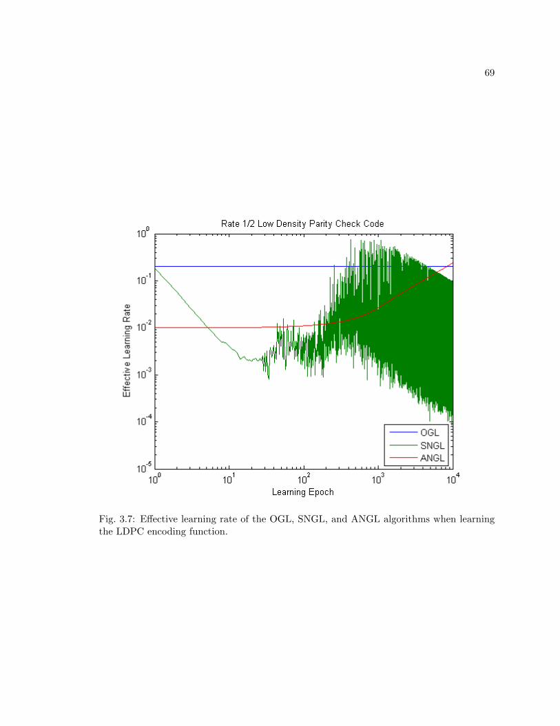
69

Fig. 3.7: Effective learning rate of the OGL, SNGL, and ANGL algorithms when learningthe LDPC encoding function.

70

of OGL. However, the performance of OGL does not improve with the SNGL algorithm’s

effective learning rate. For this problem, the Fisher information matrix used in SNGL is

a block-diagonal matrix with two 10-by-10 blocks on the main diagonal. In the ANGL

algorithm, it is a 61-by-61 matrix. These matrices are both positive definite and can be

decomposed into the product of three matrices [21]

G = VTDV. (3.13)

The matrix V is a real orthognal matrix. The matrix D is a diagonal matrix and has

the eigenvalues of G as its diagonal elements. The columns of V are the eigenvectors of

G and all are unit vectors representing directions. The eigenvalues represent how much

information is associated with each direction. Using the maximum eigenvalue to determine

an effective learning rate is good for demonstration purposes. However, it will not improve

performance of the algorithm because the directional information is missing.

These first two examples both teach a network to learn a boolean function. Each

unit in the network models a bit in a computer. The next example problem will involve

classification where each output is a probability.

3.4 The Iris Species Identification Problem

Fisher’s Iris classification data [31] has four inputs and three classes. The inputs are

the petal length, petal width, sepal length, and sepal width measured in millimeters. The

three possible classes are Iris setosa, Iris versicolor, and Iris virgnica. This data set is

interesting because it has two misclassifications. Park used this data set [35] to compare

the performance of the ANGL algorithm with that of the OGL algorithm. The network

architecture is four input nodes, four hidden nodes, and three output nodes. The transfer

function for the hidden nodes is the hyperbolic tangent. Each of the three outputs will be

the estimated probability that the given pattern belongs to Iris setosa, Iris versicolor, or

Iris virginica.

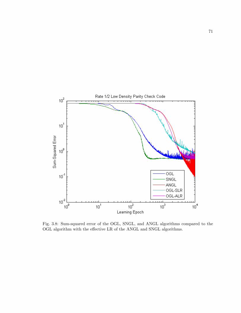
71

Fig. 3.8: Sum-squared error of the OGL, SNGL, and ANGL algorithms compared to theOGL algorithm with the effective LR of the ANGL and SNGL algorithms.

72

3.4.1 Probabilistic Model

Thus, the three outputs must always add to one. Therefore, the soft-max function will

be used

fi(a) =exp(ai)

exp(a1) + exp(a2) + exp(a3). (3.14)

The vector a in (3.14) represents the activations of the output units that are the parameters

to its soft-max transfer function.

The components of the Jacobian matrix for this function are

∂fi

∂aj=

fi(1− fi) i = j

−fifj i 6= j.

(3.15)

This function is a multivariable generalization of the logistic function in (1.2). The

probabilistic model will be

p(y|x) = [f1(A(x))]y1 [f2(A(x))]y2 [f3(A(x))]y3 . (3.16)

The activation vector is determined by A(x) = W2 tanh (W1x + b1) + b2. The com-

ponents of y = (y1, y2, y3) are each either zero or one with one and only one component

equal to one for each pattern. The likelihood of a given pattern is

`(x,y) = y1 log(f1(A(x))) + y2 log(f2(A(x))) + y3 log(f3(A(x))). (3.17)

Using the Jacobian matrix in (3.15), the derivative of the likelihood function with respect

to the activation vector a is

∂`

∂a=

f1(1− f1) −f1f2 −f1f3

−f1f2 f2(1− f2) −f2f3

−f1f3 −f2f3 f3(1− f3)

y1

f1

y2

f2

y3

f3

=

y1 − f1

y2 − f2

y3 − f3

. (3.18)

73

The score function is the gradient of the likelihod function. Thus, for the likelihood

function in (3.17), the score functions are

∂`

∂W2=

y1 − f1

y2 − f2

y3 − f3

A(x)T ,∂`

∂b2=

y1 − f1

y2 − f2

y3 − f3

, (3.19)

∂`

∂W1= tanh′(W1x + b1)WT

2

y1 − f1

y2 − f2

y3 − f3

xT , (3.20)

∂`

∂b1= tanh′(W1x + b1)WT

2

y1 − f1

y2 − f2

y3 − f3

, (3.21)

where tanh′(z) = I− diag(z)2.

This problem can be difficult to learn, even when very small random weights are chosen.

The difficulty comes because of the large numbers in the measurements. One approach can

be to translate and scale the measurements such that the mean measurements are zero and

their covariance matrix is the identity matrix. This is done by calculating the average of

each measurement from all the training patterns. Subtract the mean from each training

pattern. Use the inverse of the Cholesky decomposition [45] of the unbiased estimate of the

covariance [40] of the measurements to rescale the centered measurements. Multiplying the

centered measurements by its inverse is equivalent to dividing by the standard deviation of

a random variable.

There are 150 examples in the Iris data set. There are 50 examples of each of the three

species. To mimic the experiment performed by Park [35], 30 of each species were randomly

selected to create a training set of 90 examples. The other 60 examples will be used as a

test set. The source code for these experiments is in appendix C.

74


Figure 3.9 shows the sum-squared error of each learning epoch corresponding to the

three MLP training algorithms OGL, SNGL, and ANGL. The most striking feature of this

plot is when the ANGL algorithm starts plunging just before the thousandth epoch. Again,

this is because the ANGL algorithm does not have any mechanism to constrain the values

of the weight matrices. It does a very good job at overtraining the network for this problem.

It reaches the same SSE as the other two algorithms after 1000 epochs. The OGL algorithm

converges near the 3000th epoch while the NGL algorithm hits the same SSE near the 500th

epoch. Thus, NGL converges faster than OGL with comparable results.

Figure 3.10 shows the number of misclassified test cases. After 300 epochs, for all three

algorithms, the number of misclassified examples fluctuates between one and three. There

are two misclassified examples in Fisher’s iris data. Thus, one, two, or three errors on the

test set is considered good performance.

Figure 3.11 shows the effective learning rates of each of the algorithms. Notice that

the SNGL algorithm’s learning rate starts small and rises radically in the beginning like it

did with the XOR and LDPC problems. After that, it decreases monotonically.

Table 3.3 shows the results of the experiments. Note that even though the sum-squared

error of the ANGL algorithm is so much smaller than those of the OGL and SNGL algo-

rithms, the number of test set errors is the same in both the ANGL and SNGL algorithms.

The OGL algorithm had three test set errors, so its performance is comparable.

Thus far, the examples have been static functions. The next problem will require a

network to predict the next element of a series.

3.5 Mackey-Glass Time Series Prediction Problem

The Mackey-Glass time series (see fig. 3.12) is a chaotic series given by the recurrence

relation

x(t+ 1) = (1− b)x(t) +ax(t− τ)

1 + x(t− τ)10, (3.22)

with a = 0.2, b = 0.1, and τ = 17. The initial conditions are chosen to be x(t) = 0.9 for

75

Fig. 3.9: Sum-squared error of the OGL, ANGL, and SNGL algorithms on Fisher’s iris data.

Table 3.3: Fisher’s iris data experiment results.

Fisher’s Iris Data OGL SNGL ANGL

Hidden Units 4 4 4Initial Learning Rate 0.01 0.0098 0.01Annealed Learning Rate No Yes NoPrior Probability on Parameters Yes Yes NoHyperparameter of Prior Distribution 0.1 0.1 N/AFisher Information Matrix Size N/A (3,4) 35Adaptation Rate N/A N/A 0.001Number of Extra Parameters 0 25 1,225Final Learning Rate 0.01 4.8057e-4 0.2010Minimum Sum-Squared Error 0.3885 0.3762 1.6431e-6Test Set Classification Errors 3 2 2

76

Fig. 3.10: The number of misclassified test case of the OGL, ANGL, and SNGL algorithmson Fisher’s iris data.

77

Fig. 3.11: The effective learning rate of the OGL, ANGL, and SNGL algorithms on Fisher’siris data.

78

1 ≤ t ≤ τ . The network will try to predict x(t + 6) given the observations x(t), x(t − 6),

x(t − 12), and x(t − 18). The training set is elements 200 through 700 and the test set is

elements 5000 through 5500.

3.5.1 Network Architecture

The network architecture has four inputs as described above. There are ten hidden units

with a hyperbolic tangent transfer function. The outputs have linear transfer functions.

Thus, the error function is

J(W1,W2,b1,b2) =700∑

t=200

(x(t+ 6)−W2 tanh (W1ξt + b1)− b2)2 , (3.23)

where

ξt =

x(t)

x(t− 6)

x(t− 12)

x(t− 18)

. (3.24)

In this experiment W1 is a 10-by-5 matrix, b1 is a 10-tuple, W2 is a 1-by-11 matrix, and

b2 is a scalar. The source code for these experiments is in appendix D.


Figure 3.13 shows the sum-squared error of the three algorithms. It takes a long time

for a network to learn this problem. The OGL algorithm gets stuck in a plateau after epoch

100. It finally begins to leave it after epoch 10,000 but doesn’t make much progress after

100,000 epochs. The ANGL algorithm breaks out of the plateau region near learning epoch

3,000. It jumps around between epochs 300 and 400 and then again between 5,000 and

6,000. After epoch 6,000, it plunges down signficiantly. The SNGL performs significantly

worse until epoch 300. After epoch 300, the algorithm bounces around erratically with

an overall downward trend. By epoch 25,000 the SNGL algorithm is starting to converge.

While ANGL and SNGL have comparable performance in the later learning epochs, they

79

Fig. 3.12: The training set of the Mackey-Glass time series prediction problem.

80

both significantly outperform OGL in this experiment.

Figure 3.14 shows the effective learning rates of the three algorithms. The learning rate

was annealed for OGL because the algorithm began to act erratically in the late learning

epochs because it was taking steps that were too large. The ANGL algorithm’s learning

rate increased slightly near the end as it began to converge to a better answer. The learning

rate for SNGL begins extremely small and remains so for the first 300 learning epochs. This

means that there was a lot of information at each point in the parameter space and small

steps were necessary to find good parameters. After epoch 300, the learning rate fluctuates

violently with a steadily decreasing envelope due to annealing that finally closes around the

90,000th epoch.

Table 3.4 shows the parameters for the three learning algorithms. Note how small the

learning rate is at the beginning for the SNGL algorithm. This simply implies that there is

a lot of information and small steps should be taken. The smallest steps are taken in the

direction with the most information and the largest steps are taken in the direction with

the least.

3.6 Nonlinear Dimension Reduction

There are several algorithms recently developed to map a non-Euclidean manifold ex-

isting in a higher-dimensional Euclidean space into a Euclidean space of a lower dimen-

sion [46–52]. For example, suppose that a set points lies on a circle with each point equally

spaced. This parametric curve can be unfolded into a line segment. Let tn = nN for

n = 0, 1, 2, . . . N , then the points on the circle can be parameterized as x1(t) = cos(2πt)

and x2(t) = sin(2πt). The source code for these experiments is in appendix E.

3.6.1 Flattening a Semicircle

The parametric curve is mapped to the real line by minimizing the distance between

points in both the higher-dimensional and lower-dimensional Euclidean spaces. The outputs

of these algorithms are the coordinates of the points in the lower-dimensional Euclidean

81

Fig. 3.13: The sum-squared error of the OGL, ANGL, and SNGL algorithms on the Mackey-Glass time series prediction problem.

Table 3.4: Mackey-Glass experiment results.

Mackey-Glass OGL SNGL ANGL

Hidden Units 10 10 10Nominal Learning Rate 1e-3 1e-3 1e-3Initial Learning Rate 1e-3 2.3137e-6 1e-3Annealed Learning Rate Yes Yes NoPrior Probability on Parameters Yes Yes NoHyperparameter of Prior Distribution 0.01 1e-3 N/AFisher Information Matrix Size N/A (1,10) 61Adaptation Rate N/A N/A 1e-5Number of Extra Parameters 0 101 3,721Final Learning Rate 1e-5 5.7206e-4 0.0023Minimum Sum-Squared Error 2.4944 0.1283 0.1127

82

Fig. 3.14: The effective learning rate of the OGL, ANGL, and SNGL algorithms on theMackey-Glass time series prediction problem.

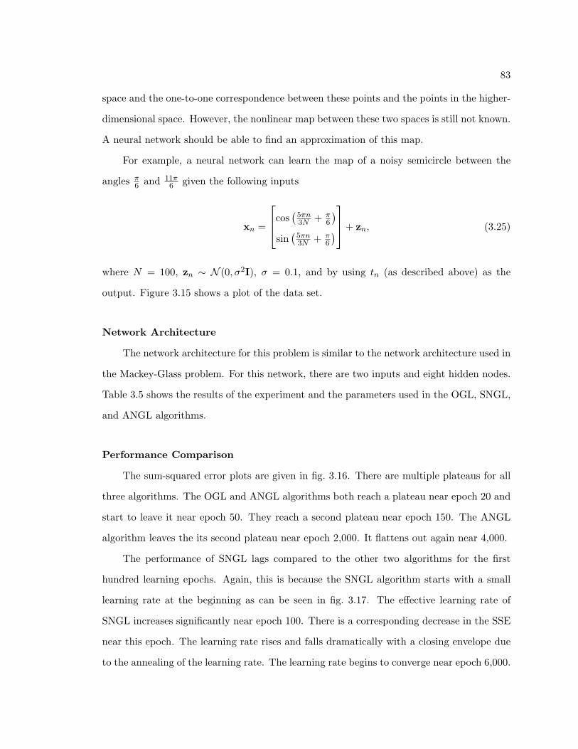
83

space and the one-to-one correspondence between these points and the points in the higher-

dimensional space. However, the nonlinear map between these two spaces is still not known.

A neural network should be able to find an approximation of this map.

For example, a neural network can learn the map of a noisy semicircle between the

angles π6 and 11π

6 given the following inputs

xn =

cos(

5πn3N + π

6

)sin(

5πn3N + π

6

)+ zn, (3.25)

where N = 100, zn ∼ N (0, σ2I), σ = 0.1, and by using tn (as described above) as the

output. Figure 3.15 shows a plot of the data set.

Network Architecture

The network architecture for this problem is similar to the network architecture used in

the Mackey-Glass problem. For this network, there are two inputs and eight hidden nodes.

Table 3.5 shows the results of the experiment and the parameters used in the OGL, SNGL,

and ANGL algorithms.

Performance Comparison

The sum-squared error plots are given in fig. 3.16. There are multiple plateaus for all

three algorithms. The OGL and ANGL algorithms both reach a plateau near epoch 20 and

start to leave it near epoch 50. They reach a second plateau near epoch 150. The ANGL

algorithm leaves the its second plateau near epoch 2,000. It flattens out again near 4,000.

The performance of SNGL lags compared to the other two algorithms for the first

hundred learning epochs. Again, this is because the SNGL algorithm starts with a small

learning rate at the beginning as can be seen in fig. 3.17. The effective learning rate of

SNGL increases significantly near epoch 100. There is a corresponding decrease in the SSE

near this epoch. The learning rate rises and falls dramatically with a closing envelope due

to the annealing of the learning rate. The learning rate begins to converge near epoch 6,000.

84

Fig. 3.15: An instance of 100 points on the semicircle between π6 and 11π

6 that has beencorrupted by additive white Gaussian noise with σ = 0.1.

Table 3.5: Nonlinear dimension reduction experiment results.

Nonlinear Dimension Reduction OGL SNGL ANGL

Hidden Units 8 8 8Nominal Learning Rate 0.001 0.001 0.001Initial Learning Rate 0.001 2.9440e-5 0.001Annealed Learning Rate Yes Yes NoPrior Probability on Parameters Yes Yes NoHyperparameter of Prior Distribution 0.01 0.01 N/AFisher Information Matrix Size N/A (1,8) 33Adaptation Rate N/A N/A 1e-4Number of Extra Parameters 0 65 1,089Final Learning Rate 1e-4 0.0086 0.0027Minimum Sum-Squared Error 0.8938 0.0759 0.4113

85

Fig. 3.16: The sum-squared error of the for the OGL, SNGL, and ANGL algorithms learningthe noisy semicircle unfolding problem.

86

There is a corresponding convergence in the SSE, too. In this experiment, SNGL performed

significantly better than OGL or ANGL.

3.6.2 Locally Linear Embedding

Locally Linear Embedding (LLE) [47] is an interesting approach because it uses linear

models to map nonlinear manifolds into a lower-dimensional space. The details of the

algorithm are beyond the scope of this work. However, a neural network can be trained to

learn the unknown mapping.

Figure 3.18 shows the S-curve [46, 47]. It is an interesting data set. Table 3.6 has the

network parameters and the experiment’s results.

Figure 3.19 shows the SSE of each learning epoch of OGL, SNGL, and ANGL. All three

make very little progress during the first 50 epochs. Significant improvements are achieved

about epoch 400. The SNGL algorithm begins its fluctuations after epoch 300. There is a

decreasing envelope due to annealing the learning rate of SNGL. The SSE converges near

epoch 70,000. Both OGL and ANGL leave their second plateau near epoch 1,000. They

reach a third plateau near epoch 10,000. Then ANGL’s SSE jumps up and then descends

further. It takes another jump near epoch 30,000 and fluctuates until epoch 50,000. It

remains steady until epoch 80,000 and then begins fluctuating again. The performance of

SNGL and ANGL is comparable. OGL performs worse as it never escapes its third plateau.

Figure 3.20 shows the effective learning rates of OGL, SNGL, and ANGL in this ex-

periment. The learning rate of OGL is held constant at 10−5 as this achieved the best

performance. This learning rate was also used on both SNGL and ANGL. The effective

learning rate of SNGL begins to decrease after the fifth epoch and continues to do so until

the hundredth. It increases dramatically between epoch 100 and 300. It then fluctuates for

the rest of its execution. The envelope of the fluctuation begins to steadily decrease near

epoch 70,000. This corresponds to where the SSE of the algorithm converges. The learning

rate for ANGL begins to increase near epoch 1,000. The slope increases after epoch 6,000

and then decreases slightly after epoch 10,000. This corresponds to the sudden jump and

then steady decrease of the SSE of the algorithm.

87

Fig. 3.17: The effective learning rate of the OGL, SNGL, and ANGL algorithms on thenoisy semicircle unfolding Problem.

Table 3.6: Locally linear embedding results.

LLE OGL SNGL ANGL

Hidden Units 5 5 5Nominal Learning Rate 1e-5 1e-3 1e-5Initial Learning Rate 1e-5 9.87e-6 1.0001e-5Annealed Learning Rate No Yes NoPrior Probability on Parameters Yes Yes NoHyperparameter of Prior Distribution 0.01 0.01 N/AFisher Information Matrix Size N/A (2,5) 32Adaptation Rate N/A N/A 1e-4Number of Extra Parameters 0 29 1,024Final Learning Rate 1e-5 6.79e-7 1.17e-4Minimum Sum-Squared Error 10.29 5.93 4.75Minimum Learning Epoch 100,000 99,964 86,023

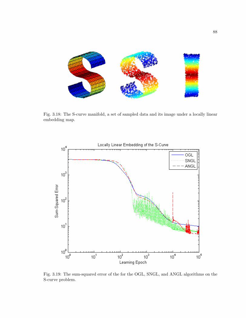
88

Fig. 3.18: The S-curve manifold, a set of sampled data and its image under a locally linearembedding map.

Fig. 3.19: The sum-squared error of the for the OGL, SNGL, and ANGL algorithms on theS-curve problem.

89

Fig. 3.20: The effective learning rate of the OGL, SNGL, and ANGL algorithms on thenoisy semicircle unfolding problem.

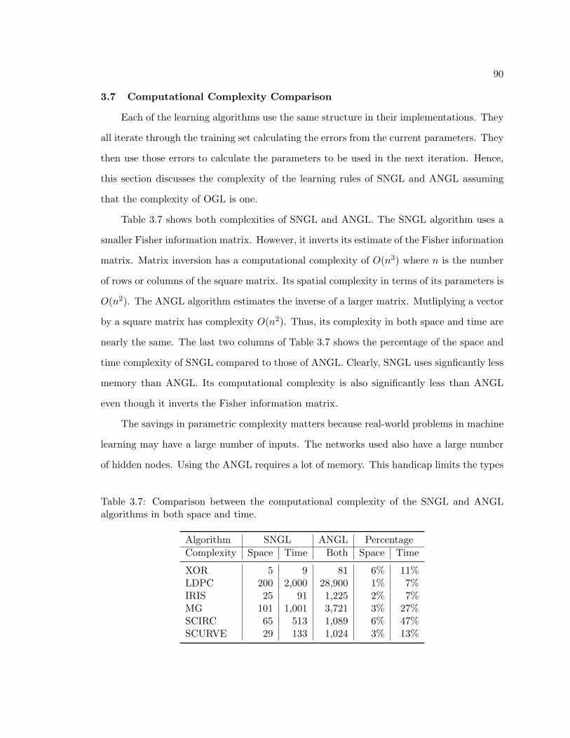
90

3.7 Computational Complexity Comparison

Each of the learning algorithms use the same structure in their implementations. They

all iterate through the training set calculating the errors from the current parameters. They

then use those errors to calculate the parameters to be used in the next iteration. Hence,

this section discusses the complexity of the learning rules of SNGL and ANGL assuming

that the complexity of OGL is one.

Table 3.7 shows both complexities of SNGL and ANGL. The SNGL algorithm uses a

smaller Fisher information matrix. However, it inverts its estimate of the Fisher information

matrix. Matrix inversion has a computational complexity of O(n3) where n is the number

of rows or columns of the square matrix. Its spatial complexity in terms of its parameters is

O(n2). The ANGL algorithm estimates the inverse of a larger matrix. Mutliplying a vector

by a square matrix has complexity O(n2). Thus, its complexity in both space and time are

nearly the same. The last two columns of Table 3.7 shows the percentage of the space and

time complexity of SNGL compared to those of ANGL. Clearly, SNGL uses signficantly less

memory than ANGL. Its computational complexity is also significantly less than ANGL

even though it inverts the Fisher information matrix.

The savings in parametric complexity matters because real-world problems in machine

learning may have a large number of inputs. The networks used also have a large number

of hidden nodes. Using the ANGL requires a lot of memory. This handicap limits the types

Table 3.7: Comparison between the computational complexity of the SNGL and ANGLalgorithms in both space and time.

Algorithm SNGL ANGL PercentageComplexity Space Time Both Space Time

XOR 5 9 81 6% 11%LDPC 200 2,000 28,900 1% 7%IRIS 25 91 1,225 2% 7%MG 101 1,001 3,721 3% 27%SCIRC 65 513 1,089 6% 47%SCURVE 29 133 1,024 3% 13%

91

of problems with which ANGL could be used. With SNGL, the memory requirements will

still impose limits but not nearly to the same extent as with ANGL.

The computational complexity savings shows that inverting a block-diagonal Fisher

information matrix in SNGL is cheaper than multiplying out the much larger inverse of the

Fisher information matrix in ANGL.

3.8 Comparison with Other Optimization Algorithms

There are two general categories of optimization algorithms: Line Search and Trust

Region [22]. Both methods determine the correct step size to take in the parameter space.

Both categories will be discussed at a high level.

3.8.1 Line Search

The line search algorithm computes a descent direction and solves a one-dimensional

optimization in that direction. A descent direction P is defined as a direction vector (or, in

the case of neural networks, a matrix) such that

〈P,∇J〉 < 0, (3.26)

where ∇J is the gradient of the objective function. The goal of a line search algorithm is

to minimize the function J in the direction of P. Thus, the one-dimensional minimization

problem can be written as a First-Order Taylor Series expansion of J about W,

J(W + αP) = J(W) + α〈P,∇J(W)〉. (3.27)

Hence, a descent direction reduces the error. Differentiating (3.27) with respect to alpha

and assigning it to zero simply restates the goal of a vanishing gradient. From this point of

view, there is no specific benefit to the line search method compared to ordinary gradient

descent because the value of α vanishes and is thus irrelevant.

92

The Second-Order Taylor Series expansion of J about W is a quadratic function of α:

µ(α) = J(W) + α〈P,∇J(W)〉+12α2 tr

(PT∇2J(W)P

). (3.28)

In this case, the derivative of (3.28) is a linear equation whose solution is

α = −tr(PT∇J(W)

)tr (PT∇2J(W)P)

. (3.29)

Let λ1 be the largest eigenvalue of the Hessian matrix∇2J . If the Hessian matrix is positive-

definite, then it is true that tr(PT∇2JP

)≤ λ1 tr

(PTP

). By choosing P = −∇J as the

descent direction, then α ≥ 1λ1

. Remember that the effective learning rate of the Simplified

Natural Gradient Learning algorithm is ηλ1

where η is the learning rate chosen a priori. If,

instead, the Hessian matrix is invertible and the descent direction is chosen to be

P = −[∇2J

]−1∇J, (3.30)

then α = 1.

An alternative method to computing the step size is numerically solving for it by

using (3.29) iteratively. For example, an initial parameter W0 is chosen with descent

direction P0 = −∇J(W0). Then α0 is computed using (3.29). The new parameter is

W1 = W0 + α0P0. The algorithm continues forward using P0 until α vanishes or the

maximum number of iterations is exceeded.

Figure 3.21 shows the performance comparison of the Line Search Method (LSM) using

the Fisher information matrix defined in (2.83) with the other algorithms. The performance

of LSM lags behind SNGL to some extent, but generally performs in a similar fashion. The

LSM algorithm performed only one iteration of the line search for each update. Thus, the

learning rule is

Wt+1 = Wt − ηtr(∇J(Wt)T∇J(Wt)

)tr (∇J(Wt)TGt∇J(Wt))

. (3.31)

Figure 3.22 shows the effective learning rates of the Line Search Method compared to

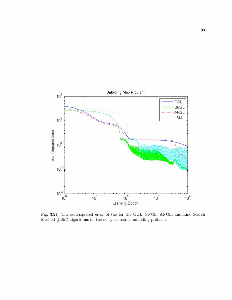
93

Fig. 3.21: The sum-squared error of the for the OGL, SNGL, ANGL, and Line SearchMethod (LSM) algorithms on the noisy semicircle unfolding problem.

94

the other algorithms. LSM and SNGL have similar curves. LSM will eventually converge

on its learning rate like SNGL, but requires more time in terms of learning epochs.

There are more sophisticated algorithms that use the Line Search Method (e.g., Con-

jugate Gradient and BFGS). These algorithms are fairly complicated and building matrix

versions would require significant time. In order to provide a more broad and general

comparison it is better to discuss trust region methods.

3.8.2 Trust Region

A Trust Region Method determines regions where the Hessian matrix is positive-

definite. The Hessian matrix is used in a Newton-type method inside the trust region.

Outside the trust region, ordinary gradient descent is used. Thus, a Trust Region Method

computes its descent direction as a linear combination of PD = −∇J and PU = −G−1∇J .

The descent direction is a function of the parameter τ such that

P(τ) =

PU τ ≤ 0

(1− τ)PU + τPD 0 < τ < 1,

PD τ ≥ 1.

(3.32)

The parameter τ is determined by maximizing

σ(τ) = ‖(1− τ)PU + τPD‖ . (3.33)

Differentiating σ(τ) and solving for τ yields,

σ′(τ) = 0 (3.34)

(1− τ) tr(PT

UPU

)+ (τ − 1

2) tr(PT

UPD

)− τ tr

(PT

DPD

)‖(1− τ)PU + τPD‖

= 0 (3.35)

τ =tr(PT

UPU

)− 1

2 tr(PT

UPD

)tr(PT

UPU

)− tr

(PT

UPD

)+ tr

(PT

DPD

) . (3.36)

95

Fig. 3.22: The effective learning rate of the OGL, SNGL, ANGL, and Line Search Method(LSM) algorithms on the noisy semicircle unfolding problem.

96

When PU and PD are orthogonal to each other, then τ is

τ =‖PU‖2

‖PU‖2 + ‖PD‖2. (3.37)

Also, when PD = βPU , then τ is

τ =1− β

2

1− β + β2. (3.38)

Figure 3.23 shows the performance of the Trust Region Method using the Fisher infor-

mation matrix compared to the Line Search Method and the other algorithms discussed in

this chapter. It starts out taking slightly larger steps than SNGL but not as steep as OGL

and ANGL. It hits a plateau at learning epoch 100 with all the other algorihms. It maintains

a smooth performance like OGL and ANGL. It finds the next lower plateau before ANGL.

Before epoch 100, the Trust Region Method behaves similarly to SNGL. That is consistent

with τ being small. After epoch 100, it behaves similarly to OGL. This is consistent with

τ being close to unity.

Figure 3.24 shows that value of the parameter τ during the course of the Trust Region

Method algorithm. Note that it starts out small and then increases during the first 100

learning epochs. When it becomes unity, the Fisher information does not contain any useful

information and only multiplies the gradient by 1α where α is the hyperparameter of the

prior distribution. Hence, the parameter τ approaches unity because the trust region has

grown significantly. Remember that the inverse Fisher information matrix is used in the

determination of the size of the trust region. Thus, when the Fisher information matrix is

nearly equal to αI, then the trust radius is 1α for almost all the nodes in each layer.

3.9 Normalizing the Error Gradient

Normalizing the gradient is frequently done in many optimization algorithms [22]. This

is done so that fixed size steps are taken in the course of the algorithms as described above.

Using a normalized gradient in neural network training to compare algorithms on a level

97

Fig. 3.23: The sum-squared error of the for the OGL, SNGL, ANGL, Line Search Method(LSM), and Trust Region Method (TRM) algorithms on the noisy semicircle unfoldingproblem.

98

Fig. 3.24: The value of the parameter τ used in the trust region method algorithm on thenoisy semicircle unfolding problem.

99

playing field has a problem: The effect of the normalization on the prior distribution of

the connection weight parameters. The purpose of this prior distribution is to mitigate

overtraining. Normalizing the gradient before subtracting the scaled-down version of the

current weights negates the effect of the prior. This is because the gradient is always

the same length (i.e., one). Normalizing the gradient after the subtraction amplifies the

noise in the data set when the gradient gets small. Thus, normalizing the gradient of the

error function should be done without subtracting the current weights multiplied by the

hyperparameter α.

The three learning algorithms OGL, ANGL, and SNGL performed similarly with nor-

malized gradients. What can be concluded from these results is that improving the per-

formance of neural network training algorithms relies more on determining when to take

larger or smaller steps than on determining the right direction.

3.10 Conclusion

A natural gradient algorithm uses the Fisher information matrix of its current parame-

ters in a Newton-type gradient descent method by replacing the Hessian matrix. The power

of natural gradient algorithms is their efficiency [33]. However, there are different ways in

which to compute the Fisher information matrix. The Simplified Natural Gradient Learn-

ing (SNGL) algorithm uses a smaller Fisher information matrix that is inverted in a batch

training algorithm. Its performance is compared to the Ordinary Gradient Learning (OGL)

algorithm and the Adaptive Natural Gradient Learing (ANGL) algorithm. The SNGL al-

gorithm performs well. The improvement comes from using a relatively low learning rate

in the beginning and a much higher rate when a better solution is found.

100

Chapter 4

Summary and Future Work

This chapter summarizes the ideas discussed in this dissertation and describes how it

might be applied or extended in the future by others. In a letter to Robert Hooke, Isaac

Newton wrote, “If I have seen further it is only by standing on the shoulders of giants” [53].

Standing on the shoulders of giants is an excellent description of this work.

4.1 Research Summary

This dissertation describes a simplification to a complex learning algorithm for multi-

layer perceptrons. Ordinary gradient descent learning works quite well for many problems.

The main problem is the plateau effect [14,33]. When a gradient descent learning algorithm

encounters a local minimum in its parameter space, the gradient gets smaller and smaller

with each succeeding step of the learning algorithm.

Amari developed an algorithm to avoid local minima by following the curvature of a

manifold in the parameter space of the perceptron [33–35, 41, 54–56]. By using a recursive

estimate of the inverse of the Fisher information matrix of the parameters, the algorithm

was able to accelerate learning in the directions with low information while not overstepping

in any directions with high information.

Training a multilayer perceptron is a nonlinear least-squares optimization problem [20,

22]. Instead of using the Hessian of the objective function, a natural gradient algorithm

uses the Fisher information matrix derived from a probability distribution that describes

the parameter space. A typical formulation for the score function (i.e., the gradient of the

log-likelihood function) is a matrix with a row for each training example and a column

for each parameter. The Fisher information matrix would then be a square matrix whose

dimension is equal to the number of parameters squared. For large problems with many

101

inputs, this dimension becomes quite large. For example, training a two-layer perceptron

with n inputs, m outputs and p hidden nodes would require O((m + n)2p2) memory cells

to store the Fisher information matrix.

4.2 Contributions

The new learning algorithm described in this dissertation was developed to reduce the

memory requirements and computational overhead of Amari’s Adaptive Natural Gradient

Learning algorithm [34]. The central idea is that the parameters are matrices and not

vectors. While it is true that matrices are isomophic to vectors [57], the action of these

parameters is the transformation of input vectors into output vectors. Thus, the direct sum

of these matrices should be used instead of stacking the rows or columns of the matrices

and then stacking the matrices. The chief benefit of this new formulation is that the Fisher

information matrix is now a block diagonal matrix. In the example from the previous

paragraph, only O(m2 + p2) memory cells would be required in a natural gradient learning

algorithm. Furthermore, inverting the matrix would only require O(m3 + p3) operations

instead of O((m+n)3p3). This new method uses less memory and less processing time than

Amari’s Adaptive Natural Gradient.

The experiments have shown that the performance of this simplified natural gradient

learning algorithm performs comparably to Amari’s Adaptive Natural Gradient Learning on

a variety of problems. They also show that the improvement to performance of these natural

gradient algorithms comes from adaptively using lower learning rates in the beginning and

then increasing them only when all the information has been filtered out of the error vectors.

4.3 Future Work

There are many areas of research in Machine Learning and elsewhere to which this

research could be applied. This section will discuss only two of them: Speech Recognition

and Nonlinear Dimension Reduction.

Speech Recognition is a very difficult problem [58–60]. A speech recognition system is

complex and a neural network usually serves the function of estimating the probability of a

102

phoneme given a few observations of the voice spectogram [61,62]. These networks are quite

large having 26 inputs for the Mel Frequency Cepstral Coefficients and their derivatives,

roughly 100 hidden units and nearly 50 outputs, one for each phoneme. Thus, a smaller

Fisher information matrix would be very important given the large size of the network. Such

a network would have 7,750 parameters. An Adaptive Natural Gradient Learning algorithm

would require 60,062,500 memory cells to store the Fisher information matrix. Using single-

precision floating-point format requiring four bytes for each variable would require 229

megabytes of memory. The Simplified Natural Gradient Learning algorithm would only

require 12,500 memory cells. There is a large amount of training data, too. Hence, the

reduction in learning cycles required to reach good performance levels will decrease overall

training time.

Nonlinear Dimension Reduction was discussed in sec. 3.6. In those experiments, the

neural network training algorithms viewed the Nonlinear Dimension Reduction method as

a black box and tried to imitate its output. There is much more that can be done. There is

some statistical data that can be gleaned from the original data and the reduced data. This

data could be used in the maximum likelihood model from which the Fisher information

matrix is derived. Doing so may improve the performance of the training algorithms signif-

icantly. The relationship between the fitting errors of the Nonlinear Dimension Reduction

algorithm and the errors of the neural network should also be investigated to discover the

confidence intervals of the neural network outputs.

4.4 Conclusion

A brief summary of this research and its potential for further research has been dis-

cussed. While not all potential research paths were enumerated, the two most promising

were briefly discussed. This final chapter concludes this dissertation.

103

References

[1] F. Mittelbach and M. Goossens, The LATEX Companion, 2nd ed., ser. Tools and Tech-niques for Computer Typesetting. Boston, MA: Addison-Wesley, 2004.

[2] T. H. Huxley, “On the hypothesis that animals are automata, and its history,” Fort-nightly Review, vol. XVL, p. 555, 1874.

[3] W. James, “Are we automata?” Mind, vol. 4, pp. 1–22, 1879.

[4] W. McColluch and W. Pitts, “A logical calculus of ideas immanent in nervous activity,”Bulletin of Mathematical Biophysics, vol. 5, pp. 115–133, 1943.

[5] D. O. Hebb, The Organization of Behavior. New York: John Wiley & Sons, 1949.

[6] A. Turing, “Intelligent machinery,” in The Essential Turing: The Ideas That GaveBirth to the Computer Age, B. J. Copeland, Ed., pp. 395–432. New York: OxfordUniversity Press, 2004.

[7] A. Turing, “Computing machinery and intelligence,” Mind, vol. LIX, no. 236, pp. 433–460, Oct. 1950.

[8] A. Turing, “Can automatic calculating machines be said to think?” in The EssentialTuring: The Ideas That Gave Birth to the Computer Age, B. J. Copeland, Ed., pp.487–506. New York: Oxford University Press, 2004.

[9] S. Parker, How the Body Works. New York: Reader’s Digest Association, 1994.

[10] K. Barnes and S. Weston, The Human Body: How It Works. New York: Barnes &Noble, 1997.

[11] M. A. Arbib, Ed., The Handbook of Brain Theory and Neural Networks, 2nd ed. Cam-bridge, MA: MIT Press, 2002.

[12] D. J. C. MacKay, Information Theory, Inference, and Learning Algorithms. NewYork: Cambridge University Press, 2003.

[13] M. Abramowitz and I. A. Stegun, Eds., Handbook of Mathematical Functions with For-mulas, Graphs, and Mathematical Tables. Washington, DC: US Government PrintingOffice, 1972.

[14] C. M. Bishop, Neural Networks for Pattern Recognition. Oxford, UK: Oxford Univer-sity Press, 1995.

[15] M. Biehl and H. Schwarze, “Learning by online gradient descent,” Journal of Physics,vol. A, no. 28, pp. 643–656, 1995.

104

[16] S. Bos and S. Amari, “Annealed online learning in multilayer neural networks,” in On-line Learning in Neural Networks, D. Saad, Ed., pp. 209–229. New York: CambridgeUniversity Press, 1999.

[17] K. Fukumizu, “Effect of batch learning in multilayer neural networks,” in Proceedingsof 5th International Conference on Neural Information Processing (ICONIP’98), pp.67–70, 1998.

[18] T. Heskes and B. Kappen, “On-line learning processes in artificial neural networks,”in Mathematical Foundations of Neural Networks, J. Taylor, Ed., pp. 199–233. Ams-terdam, Netherlands: Elsevier, 1993.

[19] N. Murata, “A statistical study of on-line learning,” in On-line Learning in NeuralNetworks, D. Saad, Ed., pp. 63–92. New York: Cambridge University Press, 1999.

[20] R. L. Burden and J. D. Faires, Numerical Analysis, 8th ed. Pacific Grove, CA: BrooksCole, Dec. 2004.

[21] R. A. Horn and C. R. Johnson, Matrix Analysis. New York: Cambridge UniversityPress, Feb. 1990.

[22] J. Nocedal and S. J. Wright, Numerical Optimization, ser. Springer Series in OperationsResearch. New York: Springer, 1999.

[23] F. Rosenblatt, “The perceptron: A probabilistic model for information storage andorganization in the brain,” Psychological Review, vol. 65, no. 6, pp. 386–408, 1958.

[24] F. Rosenblatt, Principles of Neurodynamics: Perceptrons and the Theory of BrainMechanisms. Washington DC: Spartan Books, 1962.

[25] M. L. Minsky and S. A. Papert, Perceptrons. Cambridge, MA: MIT Press, 1969.

[26] A. M. Chen, H. Lu, and W. Luo, “On the geometry of feed-forward neural networkerror surfaces,” Neural Computation, vol. 5, no. 6, pp. 910–927, 1993.

[27] D. E. Rumelhart and J. L. McClelland, Parallel Distributed Processing. Cambridge,MA: MIT Press, 1986.

[28] R. Rojas, Neural Networks, ch. 7. New York: Springer-Verlag, 1996.

[29] M. D. Buhmann and M. J. Ablowitz, Radial Basis Functions: Theory and Implemen-tations. New York: Cambridge University Press, 2003.

[30] A. Gersho and R. M. Gray, Vector Quantization and Signal Compression, 1st ed. NewYork: Springer, 1991.

[31] R. A. Fisher, “The use of multiple measurements in taxonomic problems,” Annals ofEugenics, no. 7, pp. 179–188, 1936.

[32] E. Anderson, “The irises of the gasp peninsula,” Bulletin of the American Iris Society,no. 59, pp. 2–5, 1935.

105

[33] S. Amari, “Natural gradient works efficiently in learning,” Neural Computation, vol. 10,no. 2, pp. 251–276, 1998.

[34] S. Amari, H. Park, and K. Fukumizu, “Adaptive method of realizing natural gradientlearning for multilayer perceptrons,” Neural Computation, vol. 12, no. 6, pp. 1399–1409,2000.

[35] H. Park, S. Amari, and K. Fukumizu, “Adaptive natural gradient learning algorithmsfor various stochastic models,” Neural Networks, vol. 13, no. 7, pp. 755–764, 2000.

[36] G. E. P. Box and N. R. Draper, Empirical Model-Building and Response Surfaces, p.424. New York: John Wiley & Sons, 1987.

[37] R. A. Fisher, “On the mathematical foundations of theoretical statistics,” PhilosophicalTransactions of the Royal Society of London, vol. 222, pp. 309–68, 1922.

[38] G. Casella and R. L. Berger, Statistical Inference, 2nd ed. Pacific Grove, CA: DuxburyPress, 2002.

[39] H. L. V. Trees, Detection, Estimation, and Modulation Theory, Part I. New York:John Wiley & Sons, 1968.

[40] T. K. Moon and W. C. Stirling, Mathematical Methods and Algorithms for SignalProcessing. Upper Saddle River, NJ: Prentice Hall, Aug. 1999.

[41] S. Amari and H. Nagaoka, Methods of Information Geometry, ser. Translations ofMathematical Monographs, vol. 191. New York: Oxford University Press, 2000.

[42] M. K. Murray and J. W. Rice, Differential Geometry and Statistics, ser. Monographson Statistics and Applied Probability, vol. 48. London: Chapman & Hall/CRC, 1993.

[43] J. Frank, P. Cheeseman, and J. Stutz, “When gravity fails: Local search topology,”Journal of Artificial Intelligence Research, vol. 7, pp. 249–281, 1997.

[44] T. K. Moon, Error Correction Coding: Mathematical Methods and Algorithms. NewYork: Wiley-Interscience, June 2005.

[45] G. H. Golub and C. F. V. Loan, Matrix Computations, 3rd ed. Baltimore, MD: JohnsHopkins University Press, 1996.

[46] J. B. Tenenbaum, V. de Silva, and J. C. Langford, “A global geometric framework fornonlinear dimensionality reduction,” Science, vol. 290, pp. 2319–2323, Dec. 2000.

[47] S. T. Roweis and L. K. Saul, “Nonlinear dimensionality reduction by locally linearembedding,” Science, vol. 290, pp. 2323–2326, Dec. 2000.

[48] M. Balasubramanian and E. L. Schwartz, “The isomap algorithm and topological sta-bility,” Science, vol. 295, Jan. 2002.

[49] D. K. Agrafiotis and H. Xu, “A self-organizing principle for learning nonlinear man-ifolds,” in Proceedings of the National Academy of Sciences of the United States ofAmerica, vol. 99, no. 25, pp. 15 869–15 872, 2002.

106

[50] D. K. Agrafiotis, “Stochastic proximity embedding,” Journal of Computational Chem-istry, vol. 24, no. 10, pp. 1215–1221, 2003.

[51] C. M. Bachmann, T. L. Ainsworth, and R. A. Fusina, “Exploiting manifold geometryin hyperspectral imagery,” IEEE Transactions on Geoscience and Remote Sensing,vol. 43, no. 3, pp. 441–454, Mar. 2005.

[52] K. Q. Weinberger and L. K. Saul, “An introduction to nonlinear dimensionality reduc-tion by maximum variance unfolding,” in AAAI, 2006.

[53] I. Newton, Letter to Robert Hooke, Feb. 1676. Available: http://en.wikiquote.org/wiki/Isaac Newton#Sourced

[54] S. Amari, “Information geometry of the EM and em algorithms for neural networks,”Neural Networks, vol. 8, no. 9, pp. 1379–1408, 1995.

[55] S. Amari, “Neural learning in structured parameter spaces — natural riemannian gra-dient,” in Advances in Neural Information Processing Systems, M. C. Mozer, M. I.Jordan, and T. Petsche, Eds., vol. 9, p. 127. Cambridge, MA: The MIT Press, 1997.

[56] S. Amari, H. Park, and T. Ozeki, Geometrical singularities in the neuromanifold ofmultilayer perceptrons, no. 14. Cambridge, MA: MIT Press, 2002.

[57] G. L. Bradley, A Primer of Linear Algebra. Upper Saddle River, NJ: Prentice Hall,1975.

[58] L. Rabiner and B.-H. Juang, Fundamentals of Speech Recognition. Upper SaddleRiver, NJ: Prentice Hall, 1993.

[59] F. Jelinek, Statistical Methods for Speech Recognition. Upper Saddle River, NJ: Pren-tice Hall, 1998.

[60] X. Huang, A. Acero, and H.-W. Hon, Spoken Language Processing: A Guide to Theory,Algorithm and System Development. Upper Saddle River, NJ: Prentice Hall, 2001.

[61] J.-P. Hosom, R. Cole, and M. Fanty, “Speech recognition using neuralnetworks,” Center for Spoken Language Understanding (CSLU) Oregon GraduateInstitute of Science and Technology, Technical Report, July 1999. Available:http://cslu.cse.ogi.edu/tutordemos/nnet recog/recog.html

[62] J.-P. Hosom, J. de Villiers, R. Cole, M. Fanty, J. Schalkwyk, Y. Yan, andW. Wei, “Training hidden markov model/artificial neural network (hmm/ann)hybrids for automatic speech recognition (asr),” Center for Spoken LanguageUnderstanding (CSLU) OGI School of Science and Engineering (OGI) OregonHealth and Science University (OHSU), Technical Report, Feb. 2006. Available:http://speech.bme.ogi.edu/tutordemos/nnet training/tutorial.html

107

Appendices

108

Appendix AMATLAB Code for the Exclusive OR (XOR) Experiment

The MATLAB code for the Ordinary Gradient Learning, Simplified Natural GradientLearning and Adaptive Natural Gradient Learning algorithms that learn the XOR functionare included in this section.

A.1 Ordinary Gradient Learning

%%%%%%%%%%%%%%%%%%%%%%%%%%%%%%%%%%%%%%%%%%%%%%%%%%%%%%%%%%%%%%%%%%%% This code trains a 2-2-1 network to learn the XOR function.% It uses the Ordinary Gradient Learning Algorithm (OGL).%%%%%%%%%%%%%%%%%%%%%%%%%%%%%%%%%%%%%%%%%%%%%%%%%%%%%%%%%%%%%%%%%%%

% The number of learning epochsL = 10000;

% The learning rateeta = 0.25;

% Weight decay ratealpha = 1e-2;

% Number of hidden nodesq = 2;

% Target valuest = [ -1 ; 1 ; 1 ; -1 ];

% Input vectorsx = [-1 -1 ; -1 1 ; 1 -1 ; 1 1 ];

% Number of training examplesm = length(t);

% Number of inputsn = size(x,2);

% Number of outputsk = size(t,2);

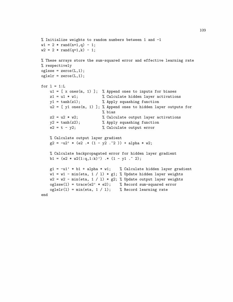
109

% Initialize weights to random numbers between 1 and -1w1 = 2 * rand(n+1,q) - 1;w2 = 2 * rand(q+1,k) - 1;

% These arrays store the sum-squared error and effective learning rate% respectivelyoglsse = zeros(L,1);oglelr = zeros(L,1);

for l = 1:Lu1 = [ x ones(m, 1) ]; % Append ones to inputs for biasesz1 = u1 * w1; % Calculate hidden layer activationsy1 = tanh(z1); % Apply squashing functionu2 = [ y1 ones(m, 1) ]; % Append ones to hidden layer outputs for

% biasz2 = u2 * w2; % Calculate output layer activationsy2 = tanh(z2); % Apply squashing functione2 = t - y2; % Calculate output error

% Calculate output layer gradientg2 = -u2’ * (e2 .* (1 - y2 .^2 )) + alpha * w2;

% Calculate backpropagated error for hidden layer gradientb1 = (e2 * w2(1:q,1:k)’) .* (1 - y1 .^ 2);

g1 = -u1’ * b1 + alpha * w1; % Calculate hidden layer gradientw1 = w1 - min(eta, 1 / l) * g1; % Update hidden layer weightsw2 = w2 - min(eta, 1 / l) * g2; % Update output layer weightsoglsse(l) = trace(e2’ * e2); % Record sum-squared erroroglelr(l) = min(eta, 1 / l); % Record learning rate

end

110

A.2 Simplified Natural Gradient Learning

%%%%%%%%%%%%%%%%%%%%%%%%%%%%%%%%%%%%%%%%%%%%%%%%%%%%%%%%%%%%%%%%%%%%%% This code trains a 2-2-1 network to learn the XOR function.% It uses the Simplified Natural Gradient Learning Algorithm (SNGL).%%%%%%%%%%%%%%%%%%%%%%%%%%%%%%%%%%%%%%%%%%%%%%%%%%%%%%%%%%%%%%%%%%%%%

% The number of learning epochsL = 10000;

% The learning rateeta = 0.25;

% The weight decay ratealpha = 1e-2;

% The number of hidden nodesq = 2;

% The target valuest = [ -1 ; 1 ; 1 ; -1 ];

% The input vectorsx = [-1 -1 ; -1 1 ; 1 -1 ; 1 1 ];

% The number of training examplesm = length(t);

% The number of inputsn = size(x,2);

% The number of outputsk = size(t,2);

% Initialize weights to random numbers between 1 and -1w1 = 0.2 * rand(n+1,q) - 0.1;w2 = 0.2 * rand(q+1,k) - 0.1;

% These arrays store the sum-squared error and effective learning rate% respectivelysnglsse = zeros(L,1);snglelr = zeros(L,1);

for l = 1:L

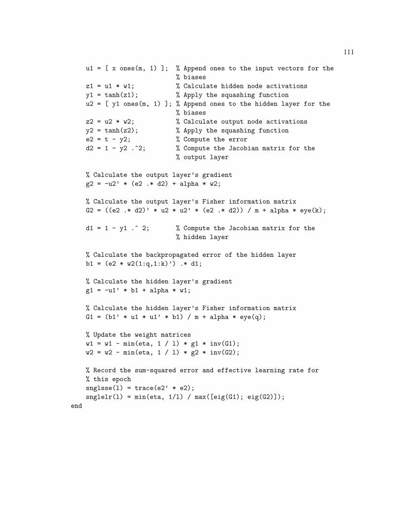
111

u1 = [ x ones(m, 1) ]; % Append ones to the input vectors for the% biases

z1 = u1 * w1; % Calculate hidden node activationsy1 = tanh(z1); % Apply the squashing functionu2 = [ y1 ones(m, 1) ]; % Append ones to the hidden layer for the

% biasesz2 = u2 * w2; % Calculate output node activationsy2 = tanh(z2); % Apply the squashing functione2 = t - y2; % Compute the errord2 = 1 - y2 .^2; % Compute the Jacobian matrix for the

% output layer

% Calculate the output layer’s gradientg2 = -u2’ * (e2 .* d2) + alpha * w2;

% Calculate the output layer’s Fisher information matrixG2 = ((e2 .* d2)’ * u2 * u2’ * (e2 .* d2)) / m + alpha * eye(k);

d1 = 1 - y1 .^ 2; % Compute the Jacobian matrix for the% hidden layer

% Calculate the backpropagated error of the hidden layerb1 = (e2 * w2(1:q,1:k)’) .* d1;

% Calculate the hidden layer’s gradientg1 = -u1’ * b1 + alpha * w1;

% Calculate the hidden layer’s Fisher information matrixG1 = (b1’ * u1 * u1’ * b1) / m + alpha * eye(q);

% Update the weight matricesw1 = w1 - min(eta, 1 / l) * g1 * inv(G1);w2 = w2 - min(eta, 1 / l) * g2 * inv(G2);

% Record the sum-squared error and effective learning rate for% this epochsnglsse(l) = trace(e2’ * e2);snglelr(l) = min(eta, 1/l) / max([eig(G1); eig(G2)]);

end

112

A.3 Adaptive Natural Gradient Learning

%%%%%%%%%%%%%%%%%%%%%%%%%%%%%%%%%%%%%%%%%%%%%%%%%%%%%%%%%%%%%%%%%%%%% This code trains a 2-2-1 network to learn the XOR function.% It uses the Amari’s Adaptive Natural Gradient Learning algorithm% (ANGL).%%%%%%%%%%%%%%%%%%%%%%%%%%%%%%%%%%%%%%%%%%%%%%%%%%%%%%%%%%%%%%%%%%%%

% Number of learning epochsL = 10000;

% Learning rateeta = 0.25;

% Adaptation ratedelta = 0.1;

% Number of hidden nodesq = 2;

% Target valuest = [ -1 ; 1 ; 1 ; -1 ];

% Input vectorsx = [-1 -1 ; -1 1 ; 1 -1 ; 1 1 ];

% Number of training examplesm = length(t);

% Number of inputsn = size(x,2);

% Number of outputsk = size(t,2);

% Initialize weights to random numbers between 1 and -1.w1 = 2 * rand(n+1,q) - 1;w2 = 2 * rand(q+1,k) - 1;

% Record the sum-squared error and effective learning rate for each% epoch.anglsse = zeros(L,1);anglelr = zeros(L,1);

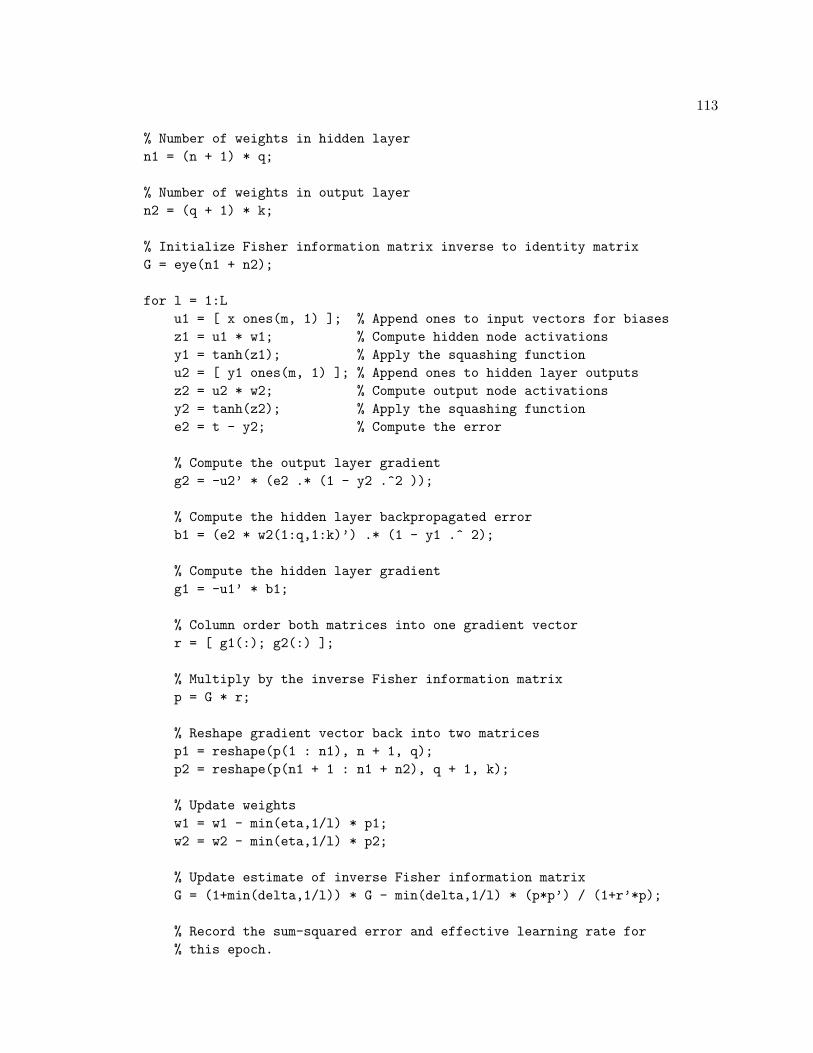
113

% Number of weights in hidden layern1 = (n + 1) * q;

% Number of weights in output layern2 = (q + 1) * k;

% Initialize Fisher information matrix inverse to identity matrixG = eye(n1 + n2);

for l = 1:Lu1 = [ x ones(m, 1) ]; % Append ones to input vectors for biasesz1 = u1 * w1; % Compute hidden node activationsy1 = tanh(z1); % Apply the squashing functionu2 = [ y1 ones(m, 1) ]; % Append ones to hidden layer outputsz2 = u2 * w2; % Compute output node activationsy2 = tanh(z2); % Apply the squashing functione2 = t - y2; % Compute the error

% Compute the output layer gradientg2 = -u2’ * (e2 .* (1 - y2 .^2 ));

% Compute the hidden layer backpropagated errorb1 = (e2 * w2(1:q,1:k)’) .* (1 - y1 .^ 2);

% Compute the hidden layer gradientg1 = -u1’ * b1;

% Column order both matrices into one gradient vectorr = [ g1(:); g2(:) ];

% Multiply by the inverse Fisher information matrixp = G * r;

% Reshape gradient vector back into two matricesp1 = reshape(p(1 : n1), n + 1, q);p2 = reshape(p(n1 + 1 : n1 + n2), q + 1, k);

% Update weightsw1 = w1 - min(eta,1/l) * p1;w2 = w2 - min(eta,1/l) * p2;

% Update estimate of inverse Fisher information matrixG = (1+min(delta,1/l)) * G - min(delta,1/l) * (p*p’) / (1+r’*p);

% Record the sum-squared error and effective learning rate for% this epoch.

114

anglsse(l) = trace(e2’ * e2);anglelr(l) = min(eta,1/l) * min(eig(G));

end

115

Appendix BMATLAB Code for the Low-Density Parity Check Code

Experiment

The following function is used in all three algorithms.

function y = flipbits(x,p)r = rand(size(x));i = find(r < p);z = zeros(size(x));z(i) = 1;y = mod(x + z, 2);

end

B.1 Ordinary Gradient Learning

L = 10000;alpha = 0.001;beta = 0.01;

q = 10;

x = [0 0 0 0 0; 0 0 0 0 1; 0 0 0 1 0; 0 0 0 1 1;0 0 1 0 0; 0 0 1 0 1; 0 0 1 1 0; 0 0 1 1 1;0 1 0 0 0; 0 1 0 0 1; 0 1 0 1 0; 0 1 0 1 1;0 1 1 0 0; 0 1 1 0 1; 0 1 1 1 0; 0 1 1 1 1;1 0 0 0 0; 1 0 0 0 1; 1 0 0 1 0; 1 0 0 1 1;1 0 1 0 0; 1 0 1 0 1; 1 0 1 1 0; 1 0 1 1 1;1 1 0 0 0; 1 1 0 0 1; 1 1 0 1 0; 1 1 0 1 1;1 1 1 0 0; 1 1 1 0 1; 1 1 1 1 0; 1 1 1 1 1];

c = [ 0 0 0 0 0; 1 1 1 0 0;1 1 0 1 0; 0 0 1 1 0;1 0 1 0 1; 0 1 0 0 1;0 1 1 1 1; 1 0 0 1 1;0 0 1 1 1; 1 1 0 1 1;1 1 1 0 1; 0 0 0 0 1;1 0 0 1 0; 0 1 1 1 0;0 1 0 0 0; 1 0 1 0 0;0 1 0 1 1; 1 0 1 1 1;1 0 0 0 1; 0 1 1 0 1;1 1 1 1 0; 0 0 0 1 0;0 0 1 0 0; 1 1 0 0 0;

116

0 1 1 0 0; 1 0 0 0 0;1 0 1 1 0; 0 1 0 1 0;1 1 0 0 1; 0 0 1 0 1;0 0 0 1 1; 1 1 1 1 1];

t = [c x];

[m n] = size(x);[m k] = size(t);

eta = 0.2;

w1 = 0.2 * rand(n + 1, q) - 0.1;w2 = 0.2 * rand(q + 1, k) - 0.1;

oglsse = zeros(L,1);oglelr = zeros(L,1);

for l = 1:Li = randperm(m);u1 = [x(i,:) ones(m,1)];y1 = sigmoid(u1 * w1);u2 = [y1 ones(m,1)];y2 = sigmoid(u2 * w2);

e2 = flipbits(t(i,:), beta) - y2;d2 = y2 - y2 .^ 2;g2 = -u2’ * (e2 .* d2) + alpha * w2;w2 = w2 - eta * g2;

e1 = e2 * w2(1:q,:)’;d1 = y1 - y1 .^ 2;g1 = -u1’ * (e1 .* d1) + alpha * w1;w1 = w1 - eta * g1;

oglsse(l) = trace((t(i,:) - y2)’ * (t(i,:) - y2));oglelr(l) = eta;

end

117

B.2 Simplified Natural Gradient Learning

L = 10000;alpha = 0.001;beta = 0.01;

q = 10;

x = [0 0 0 0 0; 0 0 0 0 1; 0 0 0 1 0; 0 0 0 1 1;0 0 1 0 0; 0 0 1 0 1; 0 0 1 1 0; 0 0 1 1 1;0 1 0 0 0; 0 1 0 0 1; 0 1 0 1 0; 0 1 0 1 1;0 1 1 0 0; 0 1 1 0 1; 0 1 1 1 0; 0 1 1 1 1;1 0 0 0 0; 1 0 0 0 1; 1 0 0 1 0; 1 0 0 1 1;1 0 1 0 0; 1 0 1 0 1; 1 0 1 1 0; 1 0 1 1 1;1 1 0 0 0; 1 1 0 0 1; 1 1 0 1 0; 1 1 0 1 1;1 1 1 0 0; 1 1 1 0 1; 1 1 1 1 0; 1 1 1 1 1];

c = [ 0 0 0 0 0; 1 1 1 0 0;1 1 0 1 0; 0 0 1 1 0;1 0 1 0 1; 0 1 0 0 1;0 1 1 1 1; 1 0 0 1 1;0 0 1 1 1; 1 1 0 1 1;1 1 1 0 1; 0 0 0 0 1;1 0 0 1 0; 0 1 1 1 0;0 1 0 0 0; 1 0 1 0 0;0 1 0 1 1; 1 0 1 1 1;1 0 0 0 1; 0 1 1 0 1;1 1 1 1 0; 0 0 0 1 0;0 0 1 0 0; 1 1 0 0 0;0 1 1 0 0; 1 0 0 0 0;1 0 1 1 0; 0 1 0 1 0;1 1 0 0 1; 0 0 1 0 1;0 0 0 1 1; 1 1 1 1 1];

t = [c x];


eta = 0.005;

w1 = 0.2 * rand(n + 1, q) - 0.1;w2 = 0.2 * rand(q + 1, k) - 0.1;

snglsse = zeros(L,1);snglelr = zeros(L,1);

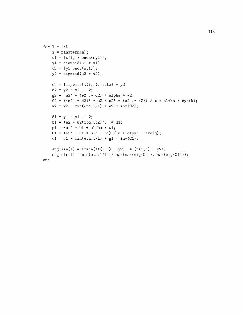
118


e2 = flipbits(t(i,:), beta) - y2;d2 = y2 - y2 .^ 2;g2 = -u2’ * (e2 .* d2) + alpha * w2;G2 = ((e2 .* d2)’ * u2 * u2’ * (e2 .* d2)) / m + alpha * eye(k);w2 = w2 - min(eta,1/l) * g2 * inv(G2);

d1 = y1 - y1 .^ 2;b1 = (e2 * w2(1:q,1:k)’) .* d1;g1 = -u1’ * b1 + alpha * w1;G1 = (b1’ * u1 * u1’ * b1) / m + alpha * eye(q);w1 = w1 - min(eta,1/l) * g1 * inv(G1);

snglsse(l) = trace((t(i,:) - y2)’ * (t(i,:) - y2));snglelr(l) = min(eta,1/l) / max(max(eig(G2)), max(eig(G1)));

end

119

B.3 Adaptive Natural Gradient Learning

L = 10000;q = 10;beta = 0.01;

x = [0 0 0 0 0; 0 0 0 0 1; 0 0 0 1 0; 0 0 0 1 1;0 0 1 0 0; 0 0 1 0 1; 0 0 1 1 0; 0 0 1 1 1;0 1 0 0 0; 0 1 0 0 1; 0 1 0 1 0; 0 1 0 1 1;0 1 1 0 0; 0 1 1 0 1; 0 1 1 1 0; 0 1 1 1 1;1 0 0 0 0; 1 0 0 0 1; 1 0 0 1 0; 1 0 0 1 1;1 0 1 0 0; 1 0 1 0 1; 1 0 1 1 0; 1 0 1 1 1;1 1 0 0 0; 1 1 0 0 1; 1 1 0 1 0; 1 1 0 1 1;1 1 1 0 0; 1 1 1 0 1; 1 1 1 1 0; 1 1 1 1 1];

c = [ 0 0 0 0 0; 1 1 1 0 0;1 1 0 1 0; 0 0 1 1 0;1 0 1 0 1; 0 1 0 0 1;0 1 1 1 1; 1 0 0 1 1;0 0 1 1 1; 1 1 0 1 1;1 1 1 0 1; 0 0 0 0 1;1 0 0 1 0; 0 1 1 1 0;0 1 0 0 0; 1 0 1 0 0;0 1 0 1 1; 1 0 1 1 1;1 0 0 0 1; 0 1 1 0 1;1 1 1 1 0; 0 0 0 1 0;0 0 1 0 0; 1 1 0 0 0;0 1 1 0 0; 1 0 0 0 0;1 0 1 1 0; 0 1 0 1 0;1 1 0 0 1; 0 0 1 0 1;0 0 0 1 1; 1 1 1 1 1];

t = [c x];


eta = 0.01;

w1 = 0.2 * rand(n + 1, q) - 0.1;w2 = 0.2 * rand(q + 1, k) - 0.1;

anglsse = zeros(L,1);anglelr = zeros(L,1);

n1 = (n + 1) * q;

120

n2 = (q + 1) * k;G = eye(n1 + n2);delta = 0.001;


e2 = flipbits(t(i,:), beta) - y2;d2 = y2 - y2 .^ 2;g2 = -u2’ * (e2 .* d2);

d1 = y1 - y1 .^ 2;b1 = (e2 * w2(1:q,1:k)’) .* d1;g1 = -u1’ * b1;

r = [g1(:); g2(:)];p = G * r;p2 = reshape(p(n1 + 1 : n1 + n2), q + 1, k);p1 = reshape(p(1 : n1), n + 1, q);w2 = w2 - eta * p2;w1 = w1 - eta * p1;G = (1 + min(delta, 1/l)) * G - min(delta, 1/l) * (p*p’) / (1 + r’*p);

anglsse(l) = trace((t(i,:) - y2)’ * (t(i,:) - y2));anglelr(l) = eta * min(diag(G));

end

121

Appendix CMATLAB Code for the Fisher’s Iris Data Experiment

The following data was used in all three algorithms.

iris_data = [50 33 14 02 1;64 28 56 22 3;65 28 46 15 2;67 31 56 24 3;63 28 51 15 3;46 34 14 03 1;69 31 51 23 3;62 22 45 15 2;59 32 48 18 2;46 36 10 02 1;61 30 46 14 2;60 27 51 16 2;65 30 52 20 3;56 25 39 11 2;65 30 55 18 3;58 27 51 19 3;68 32 59 23 3;51 33 17 05 1;57 28 45 13 2;62 34 54 23 3;77 38 67 22 3;63 33 47 16 2;67 33 57 25 3;76 30 66 21 3;49 25 45 17 3;55 35 13 02 1;67 30 52 23 3;70 32 47 14 2;64 32 45 15 2;61 28 40 13 2;48 31 16 02 1;59 30 51 18 3;55 24 38 11 2;63 25 50 19 3;64 32 53 23 3;52 34 14 02 1;49 36 14 01 1;

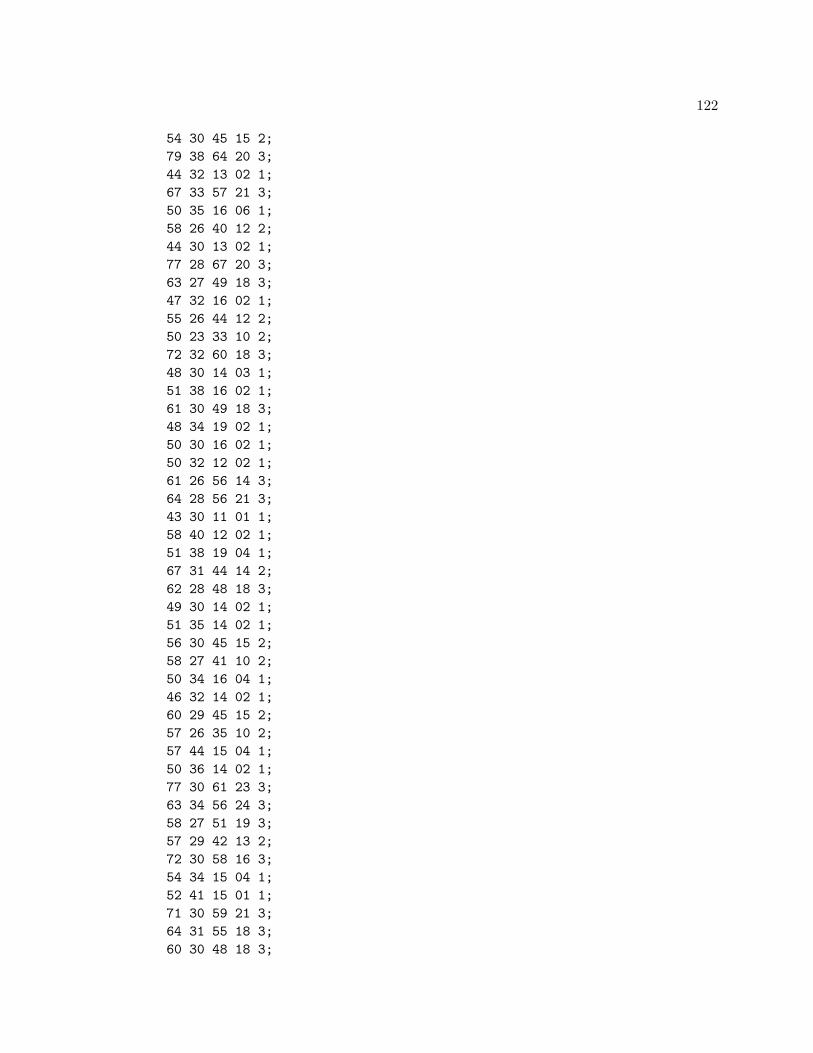
122

54 30 45 15 2;79 38 64 20 3;44 32 13 02 1;67 33 57 21 3;50 35 16 06 1;58 26 40 12 2;44 30 13 02 1;77 28 67 20 3;63 27 49 18 3;47 32 16 02 1;55 26 44 12 2;50 23 33 10 2;72 32 60 18 3;48 30 14 03 1;51 38 16 02 1;61 30 49 18 3;48 34 19 02 1;50 30 16 02 1;50 32 12 02 1;61 26 56 14 3;64 28 56 21 3;43 30 11 01 1;58 40 12 02 1;51 38 19 04 1;67 31 44 14 2;62 28 48 18 3;49 30 14 02 1;51 35 14 02 1;56 30 45 15 2;58 27 41 10 2;50 34 16 04 1;46 32 14 02 1;60 29 45 15 2;57 26 35 10 2;57 44 15 04 1;50 36 14 02 1;77 30 61 23 3;63 34 56 24 3;58 27 51 19 3;57 29 42 13 2;72 30 58 16 3;54 34 15 04 1;52 41 15 01 1;71 30 59 21 3;64 31 55 18 3;60 30 48 18 3;

123

63 29 56 18 3;49 24 33 10 2;56 27 42 13 2;57 30 42 12 2;55 42 14 02 1;49 31 15 02 1;77 26 69 23 3;60 22 50 15 3;54 39 17 04 1;66 29 46 13 2;52 27 39 14 2;60 34 45 16 2;50 34 15 02 1;44 29 14 02 1;50 20 35 10 2;55 24 37 10 2;58 27 39 12 2;47 32 13 02 1;46 31 15 02 1;69 32 57 23 3;62 29 43 13 2;74 28 61 19 3;59 30 42 15 2;51 34 15 02 1;50 35 13 03 1;56 28 49 20 3;60 22 40 10 2;73 29 63 18 3;67 25 58 18 3;49 31 15 01 1;67 31 47 15 2;63 23 44 13 2;54 37 15 02 1;56 30 41 13 2;63 25 49 15 2;61 28 47 12 2;64 29 43 13 2;51 25 30 11 2;57 28 41 13 2;65 30 58 22 3;69 31 54 21 3;54 39 13 04 1;51 35 14 03 1;72 36 61 25 3;65 32 51 20 3;61 29 47 14 2;

124

56 29 36 13 2;69 31 49 15 2;64 27 53 19 3;68 30 55 21 3;55 25 40 13 2;48 34 16 02 1;48 30 14 01 1;45 23 13 03 1;57 25 50 20 3;57 38 17 03 1;51 38 15 03 1;55 23 40 13 2;66 30 44 14 2;68 28 48 14 2;54 34 17 02 1;51 37 15 04 1;52 35 15 02 1;58 28 51 24 3;67 30 50 17 2;63 33 60 25 3;53 37 15 02 1

];

sorted_data = sortrows(iris_data, 5);

train_index = [ 1:30 51:80 101:130];test_index = [31:50 81:100 131:150];

train_data = sorted_data(train_index, 1:4);test_data = sorted_data(test_index, 1:4);

train_class = sorted_data(train_index, 5);test_class = sorted_data(test_index, 5);

I3 = eye(3);

train_target = I3(train_class, 1:3);test_target = I3(test_class, 1:3);

mu = mean(train_data(:,1:4));C = cov(train_data(:,1:4));R = chol(C);S = inv(R);x = (train_data - repmat(mu, size(train_data, 1), 1)) * S;t = train_target;z = (test_data - repmat(mu, size(test_data, 1), 1)) * S;

125

C.1 Ordinary Gradient Learning

eta = 0.01;alpha = 0.1;L = 10000;q = 4;


w1 = 0.2 * rand(n + 1, q) - 0.1;w2 = 0.2 * rand(q + 1, k) - 0.1;

oglsse = zeros(L,1);oglent = zeros(L,1);oglcnt = zeros(L,1);oglelr = zeros(L,1);

for l = 1:Li = randperm(m);u1 = [ x(i,:) ones(m,1) ];y1 = tanh(u1 * w1);u2 = [ y1 ones(m,1) ];z2 = exp(u2 * w2);y2 = diag(1 ./ sum(z2,2)) * z2;

e2 = t(i,:) - y2;g2 = -u2’ * e2 + alpha * w2;w2 = w2 - eta * g2;

b1 = (e2 * w2(1:q,:)’) .* (1 - y1 .^ 2);g1 = -u1’ * b1 + alpha * w1;w1 = w1 - eta * g1;

oglsse(l) = trace(e2’ * e2);

u1 = [ z ones(size(test_data, 1), 1) ];y1 = tanh(u1 * w1);u2 = [ y1 ones(size(test_data, 1), 1) ];v2 = exp(u2 * w2);y2 = diag(1 ./ sum(v2, 2)) * v2;

p = prod(y2 .^ test_target, 2);oglent(l) = -sum(p .* log(p)) / m;oglcnt(l) = length(find(p < 0.5));oglelr(l) = eta;

126

end

127

C.2 Simplified Natural Gradient Learning

eta = 0.01;tau = 0.5;alpha = 0.1;L = 10000;q = 4;


w1 = 0.2 * rand(n + 1, q) - 0.1;w2 = 0.2 * rand(q + 1, k) - 0.1;

snglsse = zeros(L,1);snglelr = zeros(L,1);snglent = zeros(L,1);snglcnt = zeros(L,1);

for l = 1:Li = randperm(m);u1 = [ x(i,:) ones(m,1) ];y1 = tanh(u1 * w1);u2 = [ y1 ones(m,1) ];z2 = exp(u2 * w2);y2 = diag(1 ./ sum(z2,2)) * z2;e2 = t(i,:) - y2;

g2 = -u2’ * e2 + alpha * w2;G2 = (u2’ * e2)’ * u2’ * e2 / (m - 1) + alpha * eye(k);p2 = g2 * inv(G2);w2 = w2 - min(eta, tau/l) * p2;

b1 = (e2 * w2(1:q,:)’) .* (1 - y1 .^ 2);g1 = -u1’ * b1 + alpha * w1;G1 = (u1’ * b1)’ * u1’ * b1 / (m - 1) + alpha * eye(q);p1 = g1 * inv(G1);w1 = w1 - min(eta, tau/l) * p1;

snglelr(l) = min(eta, tau/l) / max(max(eig(G1)), max(eig(G2)));snglsse(l) = trace(e2’ * e2);

u1 = [ z ones(size(test_data, 1), 1) ];y1 = tanh(u1 * w1);u2 = [ y1 ones(size(test_data, 1), 1) ];v2 = exp(u2 * w2);

128

y2 = diag(1 ./ sum(v2, 2)) * v2;

p = prod(y2 .^ test_target, 2);snglent(l) = -sum(p .* log(p)) / m;snglcnt(l) = length(find(p < 0.5));

end

129

C.3 Adaptive Natural Gradient Learning

eta = 0.01;L = 10000;q = 4;


n1 = (n+1) * q;n2 = (q+1) * k;

delta = 0.001;

w1 = 0.2 * rand(n + 1, q) - 0.1;w2 = 0.2 * rand(q + 1, k) - 0.1;

G = eye(n1 + n2);

anglsse = zeros(L,1);anglelr = zeros(L,1);anglent = zeros(L,1);anglcnt = zeros(L,1);

for l = 1:Li = randperm(m);u1 = [x(i,:) ones(m,1)];y1 = tanh(u1 * w1);u2 = [y1 ones(m,1)];z2 = exp(u2 * w2);y2 = diag(1 ./ sum(z2,2)) * z2;e2 = t(i, 1:k) - y2;g2 = -u2’ * e2;b1 = (e2 * w2(1:q, 1:k)’) .* (1 - y1 .^ 2);g1 = -u1’ * b1;r = [g1(:); g2(:)];p = G * r;G = (1 + min(delta,1/l)) * G - min(delta,1/l) * (p*p’) / (1 + r’*p);p1 = p(1:n1);p2 = p(n1+1:n1+n2);w1 = w1 - eta * reshape(p1, n+1, q);w2 = w2 - eta * reshape(p2, q+1, k);anglsse(l) = trace(e2’ * e2);anglelr(l) = eta * min(eig(G));

u1 = [ z ones(size(test_data, 1), 1) ];

130

y1 = tanh(u1 * w1);u2 = [ y1 ones(size(test_data, 1), 1) ];v2 = exp(u2 * w2);y2 = diag(1 ./ sum(v2, 2)) * v2;

pr = prod(y2 .^ test_target, 2);anglent(l) = -sum(pr .* log(pr)) / m;anglcnt(l) = length(find(pr < 0.5));

end

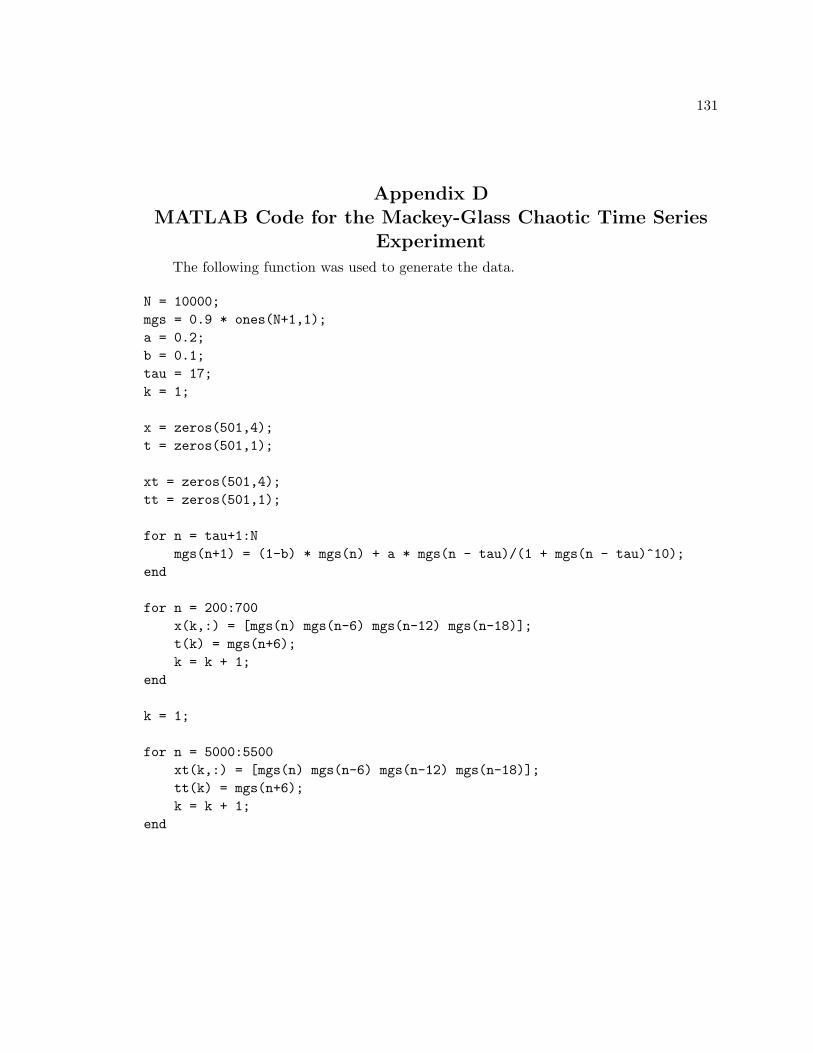
131

Appendix DMATLAB Code for the Mackey-Glass Chaotic Time Series

Experiment

The following function was used to generate the data.

N = 10000;mgs = 0.9 * ones(N+1,1);a = 0.2;b = 0.1;tau = 17;k = 1;

x = zeros(501,4);t = zeros(501,1);

xt = zeros(501,4);tt = zeros(501,1);

for n = tau+1:Nmgs(n+1) = (1-b) * mgs(n) + a * mgs(n - tau)/(1 + mgs(n - tau)^10);

end

for n = 200:700x(k,:) = [mgs(n) mgs(n-6) mgs(n-12) mgs(n-18)];t(k) = mgs(n+6);k = k + 1;

end

k = 1;

for n = 5000:5500xt(k,:) = [mgs(n) mgs(n-6) mgs(n-12) mgs(n-18)];tt(k) = mgs(n+6);k = k + 1;

end

132

D.1 Ordinary Gradient Learning

L = 100000;tau = 1;eta = 0.001;alpha = 0.01;

q = 10;


w1 = 0.2 * rand(n + 1, q) - 0.1;w2 = 0.2 * rand(q + 1, k) - 0.1;


for l = 1:Li = randperm(m);u1 = [x(i,:) ones(m,1)];y1 = tanh(u1 * w1);u2 = [y1 ones(m,1)];y2 = u2 * w2;e2 = t(i) - y2;g2 = -u2’ * e2 + alpha * w2;b1 = e2 * w2(1:q,:)’;d1 = ones(size(y1)) - y1 .^ 2;e1 = b1 .* d1;g1 = -u1’ * e1 + alpha * w1;w1 = w1 - min(eta, tau / l) * g1;w2 = w2 - min(eta, tau / l) * g2;oglsse(l) = e2’ * e2;oglelr(l) = min(eta, tau / l);

end

133

D.2 Simplified Natural Gradient Learning

L = 100000;tau = 0.1;eta = 1e-3;alpha = 0.001;

q = 10;


w1 = 0.2 * rand(n + 1, q) - 0.1;w2 = 0.2 * rand(q + 1, k) - 0.1;


for l = 1:Li = randperm(m);u1 = [x(i,:) ones(m,1)];y1 = tanh(u1 * w1);u2 = [y1 ones(m,1)];y2 = u2 * w2;e2 = t(i) - y2;g2 = -u2’ * e2 + alpha * w2;G2 = (u2’ * e2)’ * u2’ * e2 / (m - 1) + alpha * eye(k);b1 = e2 * w2(1:q,:)’;d1 = ones(size(y1)) - y1 .^ 2;e1 = b1 .* d1;g1 = -u1’ * e1 + alpha * w1;G1 = (u1’ * e1)’ * u1’ * e1 / (m - 1) + alpha * eye(q);w1 = w1 - min(eta, tau / l) * g1 * inv(G1);w2 = w2 - min(eta, tau / l) * g2 * inv(G2);snglsse(l) = e2’ * e2;snglelr(l) = min(eta, tau / l) / max(G2, max(eig(G1)));

end

134

D.3 Adaptive Natural Gradient Learning

L = 100000;eta = 1e-3;delta = 1e-5;

[m n] = size(x);[m k] = size(t);n1 = (n + 1) * q;n2 = (q + 1) * k;

q = 10;

G = eye(n1 + n2);

w1 = 0.2 * rand(n + 1, q) - 0.1;w2 = 0.2 * rand(q + 1, k) - 0.1;


for l = 1:Li = randperm(m);u1 = [x(i,:) ones(m,1)];y1 = tanh(u1 * w1);u2 = [y1 ones(m,1)];y2 = u2 * w2;e2 = t(i) - y2;g2 = -u2’ * e2;g1 = -u1’ * ((e2 * w2(1:q,1:k)’) .* (1 - y1 .^ 2));r = [g1(:); g2(:)];p = G * r;G = (1 + min(delta,1/l)) * G - min(delta,1/l) * (p*p’) / (1 + r’*p);p1 = p(1:n1);p2 = p(n1 + 1 : n1 + n2);w1 = w1 - eta * reshape(p1, n + 1, q);w2 = w2 - eta * reshape(p2, q + 1, k);anglsse(l) = e2’ * e2;anglelr(l) = eta * min(diag(G));

end

135

Appendix EMATLAB Code for the Semicircle and S-Curve Unfolding

Experiments

t = 0:0.01:1;t = t(:);m = length(t);angle = 5*pi*t/3 + pi/6;x = [cos(angle) sin(angle)] + 0.1 * randn(m,2);

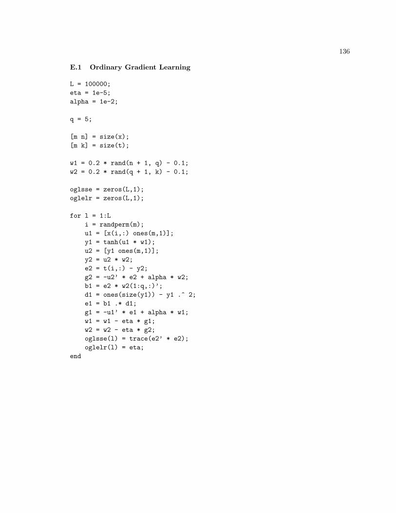
136

E.1 Ordinary Gradient Learning

L = 100000;eta = 1e-5;alpha = 1e-2;

q = 5;


w1 = 0.2 * rand(n + 1, q) - 0.1;w2 = 0.2 * rand(q + 1, k) - 0.1;


for l = 1:Li = randperm(m);u1 = [x(i,:) ones(m,1)];y1 = tanh(u1 * w1);u2 = [y1 ones(m,1)];y2 = u2 * w2;e2 = t(i,:) - y2;g2 = -u2’ * e2 + alpha * w2;b1 = e2 * w2(1:q,:)’;d1 = ones(size(y1)) - y1 .^ 2;e1 = b1 .* d1;g1 = -u1’ * e1 + alpha * w1;w1 = w1 - eta * g1;w2 = w2 - eta * g2;oglsse(l) = trace(e2’ * e2);oglelr(l) = eta;

end

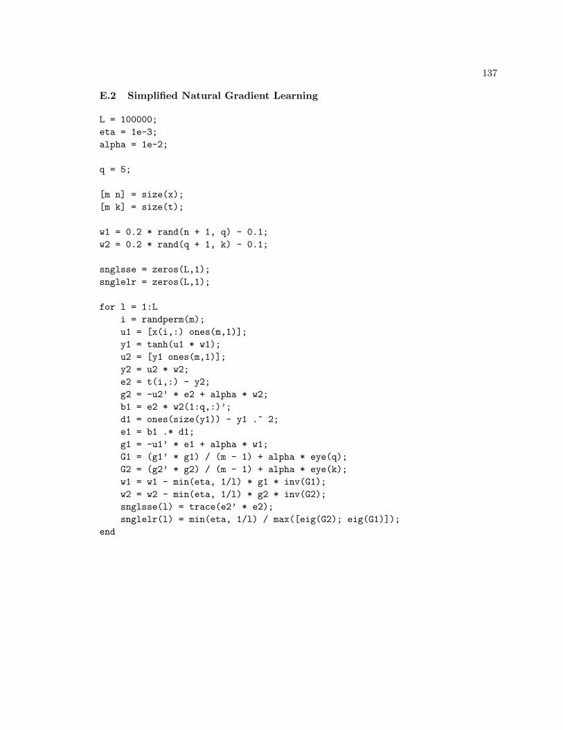
137

E.2 Simplified Natural Gradient Learning

L = 100000;eta = 1e-3;alpha = 1e-2;

q = 5;


w1 = 0.2 * rand(n + 1, q) - 0.1;w2 = 0.2 * rand(q + 1, k) - 0.1;


for l = 1:Li = randperm(m);u1 = [x(i,:) ones(m,1)];y1 = tanh(u1 * w1);u2 = [y1 ones(m,1)];y2 = u2 * w2;e2 = t(i,:) - y2;g2 = -u2’ * e2 + alpha * w2;b1 = e2 * w2(1:q,:)’;d1 = ones(size(y1)) - y1 .^ 2;e1 = b1 .* d1;g1 = -u1’ * e1 + alpha * w1;G1 = (g1’ * g1) / (m - 1) + alpha * eye(q);G2 = (g2’ * g2) / (m - 1) + alpha * eye(k);w1 = w1 - min(eta, 1/l) * g1 * inv(G1);w2 = w2 - min(eta, 1/l) * g2 * inv(G2);snglsse(l) = trace(e2’ * e2);snglelr(l) = min(eta, 1/l) / max([eig(G2); eig(G1)]);

end

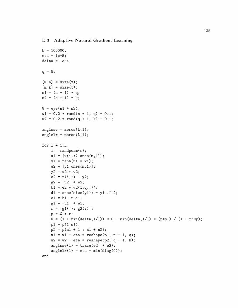
138

E.3 Adaptive Natural Gradient Learning

L = 100000;eta = 1e-5;delta = 1e-4;

q = 5;

[m n] = size(x);[m k] = size(t);n1 = (n + 1) * q;n2 = (q + 1) * k;

G = eye(n1 + n2);w1 = 0.2 * rand(n + 1, q) - 0.1;w2 = 0.2 * rand(q + 1, k) - 0.1;


for l = 1:Li = randperm(m);u1 = [x(i,:) ones(m,1)];y1 = tanh(u1 * w1);u2 = [y1 ones(m,1)];y2 = u2 * w2;e2 = t(i,:) - y2;g2 = -u2’ * e2;b1 = e2 * w2(1:q,:)’;d1 = ones(size(y1)) - y1 .^ 2;e1 = b1 .* d1;g1 = -u1’ * e1;r = [g1(:); g2(:)];p = G * r;G = (1 + min(delta,1/l)) * G - min(delta,1/l) * (p*p’) / (1 + r’*p);p1 = p(1:n1);p2 = p(n1 + 1 : n1 + n2);w1 = w1 - eta * reshape(p1, n + 1, q);w2 = w2 - eta * reshape(p2, q + 1, k);anglsse(l) = trace(e2’ * e2);anglelr(l) = eta * min(diag(G));

end

139

Vita

Michael R. Bastian

Published Conference Papers

• Sobolev Gradients and Neural Networks, Michael R. Bastian, Jacob H. Gunther

and Todd K. Moon, IEEE Int. Conf. on Acoustics, Speech and Signal Processing

(ICASSP), 2008.

• An Improvement to the Natural Gradient Learning Algorithm for Multilayer Percep-

trons, Michael R. Bastian, Jacob H. Gunther and Todd K. Moon, IEEE Int. Conf.

on Acoustics, Speech and Signal Processing (ICASSP), 2005.

• Color quantization and dithering gamuts, B. Morse, T. Howard, S. Larson, M. Bastian

and E. Mortensen, Int. Conf. on Signal and Image Processing (SIP), 1999.

• A Bayesian exclusionary rule for Hough transforms, B. Morse, D. Ashton and M.

Bastian, Int. Conf. on Computer Vision, Pattern Recognition, and Image Processing

(CVPRIP) in Joint Conference on Information Sciences (JCIS), 1999.

Documents

NEURAL NETWORKS AND THE NATURAL GRADIENT by · Neural Networks and the Natural Gradient by ... C.1 Ordinary Gradient Learning ... 1.10 The plot of the output of a double-layer perceptron