Gradient Centralization: A New OptimizationTechnique for Deep Neural Networks

Hongwei Yong1,2, Jianqiang Huang2, Xiansheng Hua2, and Lei Zhang1,2

1 Department of Computing, The Hong Kong Polytechnic University{cshyong,cslzhang}@comp.polyu.edu.hk

2 DAMO Academy, Alibaba Group{jianqiang.jqh,huaxiansheng}@gmail.com

Abstract. Optimization techniques are of great importance to effec-tively and efficiently train a deep neural network (DNN). It has beenshown that using the first and second order statistics (e.g., mean andvariance) to perform Z-score standardization on network activations orweight vectors, such as batch normalization (BN) and weight standard-ization (WS), can improve the training performance. Different from theseexisting methods that mostly operate on activations or weights, we presenta new optimization technique, namely gradient centralization (GC), whichoperates directly on gradients by centralizing the gradient vectors tohave zero mean. GC can be viewed as a projected gradient descentmethod with a constrained loss function. We show that GC can reg-ularize both the weight space and output feature space so that it canboost the generalization performance of DNNs. Moreover, GC improvesthe Lipschitzness of the loss function and its gradient so that the trainingprocess becomes more efficient and stable. GC is very simple to imple-ment and can be easily embedded into existing gradient based DNNoptimizers with only one line of code. It can also be directly used to fine-tune the pre-trained DNNs. Our experiments on various applications,including general image classification, fine-grained image classification,detection and segmentation, demonstrate that GC can consistently im-prove the performance of DNN learning. The code of GC can be foundat https://github.com/Yonghongwei/Gradient-Centralization.

Keywords: Deep network optimization, gradient descent

1 Introduction

The broad success of deep learning largely owes to the recent advances on large-scale datasets [43], powerful computing resources (e.g., GPUs and TPUs), sophis-ticated network architectures [15,16] and optimization algorithms [4,24]. Amongthese factors, the efficient optimization techniques, such as stochastic gradientdescent (SGD) with momentum [38], Adagrad [10] and Adam [24], make it pos-sible to train very deep neural networks (DNNs) with a large-scale dataset, andconsequently deliver more powerful and robust DNN models in practice. Thegeneralization performance of the trained DNN models as well as the efficiencyof training process depend essentially on the employed optimization techniques.

arX

iv:2

004.

0146

1v2

[cs

.CV

] 8

Apr

202

0

2 H. Yong et al.

There are two major goals for a good DNN optimizer: accelerating the train-ing process and improving the model generalization capability. The first goalaims to spend less time and cost to reach a good local minima, while the secondgoal aims to ensure that the learned DNN model can make accurate predictionson test data. A variety of optimization algorithms [38,10,24,10,24] have beenproposed to achieve these goals. SGD [4,5] and its extension SGD with momen-tum (SGDM) [38] are among the most commonly used ones. They update theparameters along the opposite direction of their gradients in one training step.Most of the current DNN optimization methods are based on SGD and improveSGD to better overcome the gradient vanishing or explosion problems. A fewsuccessful techniques have been proposed, such as weight initialization strate-gies [11,14], efficient active functions (e.g., ReLU [35]), gradient clipping [36,37],adaptive learning rate optimization algorithms [10,24], and so on.

In addition to the above techniques, the sample/feature statistics such asmean and variance can also be used to normalize the network activations orweights to make the training process more stable. The representative methodsoperating on activations include batch normalization (BN) [19], instance nor-malization (IN) [47,18], layer normalization (LN) [29] and group normalization(GN) [51]. Among them, BN is the most widely used optimization techniquewhich normalizes the features along the sample dimension in a mini-batch fortraining. BN smooths the optimization landscape [45] and it can speed up thetraining process and boost model generalization performance when a properbatch size is used [53,15]. However, BN works not very well when the trainingbatch size is small, which limits its applications to memory consuming tasks,such as object detection [13,42], video classification [21,2], etc.

Another line of statistics based methods operate on weights. The representa-tive ones include weight normalization (WN) [44,17] and weight standardization(WS) [39]. These methods re-parameterize weights to restrict weight vectorsduring training. For example, WN decouples the length of weight vectors fromtheir direction to accelerate the training of DNNs. WS uses the weight vectors’mean and variance to standardize them to have zero mean and unit variance.Similar to BN, WS can also smooth the loss landscape and speed up training.Nevertheless, such methods operating on weight vectors cannot directly adoptthe pre-trained models (e.g., on ImageNet) because their weights may not meetthe condition of zero mean and unit variance.

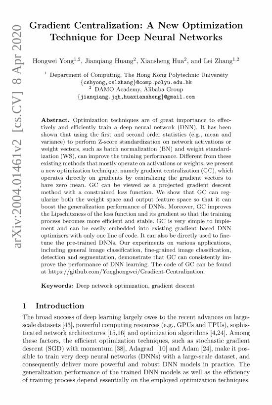
Different from the above techniques which operate on activations or weightvectors, we propose a very simple yet effective DNN optimization technique,namely gradient centralization (GC), which operates on the gradients of weightvectors. As illustrated in Fig. 1(a), GC simply centralizes the gradient vectorsto have zero mean. It can be easily embedded into the current gradient basedoptimization algorithms (e.g., SGDM [38], Adam [24]) using only one line ofcode. Though simple, GC demonstrates various desired properties, such as ac-celerating the training process, improving the generalization performance, andthe compatibility for fine-tuning pre-trained models. The main contributions ofthis paper are highlighted as follows:

Gradient Centralization 3

(a) (b)

Fig. 1. (a) Sketch map for using gradient centralization (GC). W is the weight, L is theloss function, ∇WL is the gradient of weight, and ΦGC(∇WL) is the centralized gradi-ent. It is very simple to embed GC into existing network optimizers by replacing ∇WLwith ΦGC(∇WL). (b) Illustration of the GC operation on gradient matrix/tensor ofweights in the fully-connected layer (left) and convolutional layer (right). GC computesthe column/slice mean of gradient matrix/tensor and centralizes each column/slice tohave zero mean.

• We propose a new general network optimization technique, namely gradientcentralization (GC), which can not only smooth and accelerate the trainingprocess of DNN but also improve the model generalization performance.

• We analyze the theoretical properties of GC, and show that GC constrainsthe loss function by introducing a new constraint on weight vector, whichregularizes both the weight space and output feature space so that it canboost model generalization performance. Besides, the constrained loss func-tion has better Lipschitzness than the original one, which makes the trainingprocess more stable and efficient.

Finally, we perform comprehensive experiments on various applications, in-cluding general image classification, fine-grained image classification, object de-tection and instance segmentation. The results demonstrate that GC can consis-tently improve the performance of learned DNN models in different applications.It is a simple, general and effective network optimization method.

2 Related Work

In order to accelerate the training and boost the generalization performance ofDNNs, a variety of optimization techniques [19,51,44,39,38,36] have been pro-posed to operate on activation, weight and gradient. In this section we brieflyreview the related work from these three aspects.

Activation: The activation normalization layer has become a common set-ting in DNN, such as batch normalization (BN) [19] and group normalization(GN) [51]. BN was originally introduced to solve the internal covariate shift bynormalizing the activations along the sample dimension. It allows higher learning

4 H. Yong et al.

rates [3], accelerates the training speed and improves the generalization accu-racy [33,45]. However, BN does not perform well when the training batch sizeis small, and GN is proposed to address this problem by normalizing the acti-vations or feature maps in a divided group for each input sample. In addition,layer normalization (LN) [29] and instance normalization (IN) [47,18] have beenproposed for RNN and style transfer learning, respectively.

Weight: Weight normalization (WN) [44] re-parameterizes the weight vec-tors and decouples the length of a weight vector from its direction. It speeds upthe convergence of SGDM algorithm to a certain degree. Weight standardiza-tion (WS) [39] adopts the Z-score standardization to re-parameterize the weightvectors. Like BN, WS can also smooth the loss landscape and improve trainingspeed. Besides, binarized DNN [40,9,8] quantifies the weight into binary values,which can improve the generalization capability for certain DNNs. However, ashortcoming of those methods operating on weights is that they cannot be di-rectly used to fine-tune pre-trained models since the pre-trained weight may notmeet their constraints. As a consequence, we have to design specific pre-trainingmethods for them in order to fine-tune the model.

Gradient: A commonly used operation on gradient is to compute the mo-mentum of gradient [38]. By using the momentum of gradient, SGDM acceleratesSGD in the relevant direction and dampens oscillations. Besides, L2 regulariza-tion based weight decay, which introduces L2 regularization into the gradientof weight, has long been a standard trick to improve the generalization perfor-mance of DNNs [27,54]. To make DNN training more stable and avoid gradientexplosion, gradient clipping [36,37,1,23] has been proposed to train a very deepDNNs. In addition, the projected gradient methods [12,28] and Riemannian ap-proach [7,49] project the gradient on a subspace or a Riemannian manifold toregularize the learning of weights.

3 Gradient Centralization

3.1 Motivation

BN [19] is a powerful DNN optimization technique, which uses the first andsecond order statistics to perform Z-score standardization on activations. It hasbeen shown in [45] that BN reduces the Lipschitz constant of loss function andmakes the gradients more Lipschitz smooth so that the optimization landscapebecomes smoother. WS [39] can also reduce the Lipschitzness of loss function andsmooth the optimization landscape through Z-score standardization on weightvectors. BN and WS operate on activations and weight vectors, respectively, andthey implicitly constrict the gradient of weights, which improves the Lipschitzproperty of loss for optimization.

Apart from operating on activation and weight, can we directly operate ongradient to make the training process more effective and stable? One intuitiveidea is that we use Z-score standardization to normalize gradient, like what hasbeen done by BN and WS on activation and weight. Unfortunately, we foundthat normalizing gradient cannot improve the stability of training. Instead, we

Gradient Centralization 5

propose to compute the mean of gradient vectors and centralize the gradientsto have zero mean. As we will see in the following development, the so calledgradient centralization (GC) method can have good Lipschitz property, smooththe DNN training and improve the model generalization performance.

3.2 Notations

We define some basic notations. For fully connected layers (FC layers), the weightmatrix is denoted as Wfc ∈ RCin×Cout , and for convolutional layers (Convlayers) the weight tensor is denoted as Wconv ∈ RCin×Cout×(k1k2), where Cin isthe number of input channels, Cout is the number of output channels, and k1, k2are the kernel size of convolution layers. For the convenience of expression, weunfold the weight tensor of Conv layer into a matrix/tensor and use a unifiednotation W ∈ RM×N for weight matrix in FC layer (W ∈ RCin×Cout) andConv layers (W ∈ R(Cink1k2)×Cout). Denote by wi ∈ RM (i = 1, 2, ..., N) thei-th column vector of weight matrix W and L the objective function. ∇WLand ∇wiL denote the gradient of L w.r.t. the weight matrix W and weightvector wi, respectively. The size of gradient matrix ∇WL is the same as weightmatrix W. Let X be the input activations for this layer and WTX be its outputactivations. e = 1√

M1 denotes an M dimensional unit vector and I ∈ RM×M

denotes an identity matrix.

3.3 Formulation of GC

For a FC layer or a Conv layer, suppose that we have obtained the gradientthrough backward propagation, then for a weight vector wi whose gradient is∇wiL (i = 1, 2, ..., N), the GC operator, denoted by ΦGC , is defined as follows:

ΦGC(∇wiL) = ∇wiL − µ∇wiL (1)

where µ∇wiL = 1

M

∑Mj=1∇Wi,jL. The formulation of GC is very simple. As

shown in Fig. 1(b), we only need to compute the mean of the column vectors ofthe weight matrix, and then remove the mean from each column vector. We canalso have a matrix formulation of Eq. (1):

ΦGC(∇WL) = P∇WL, P = I− eeT (2)

The physical meaning of P will be explained later in Section 4.1. In practicalimplementation, we can directly remove the mean value from each weight vectorto accomplish the GC operation. The computation is very simple and efficient.

3.4 Embedding of GC to SGDM/Adam

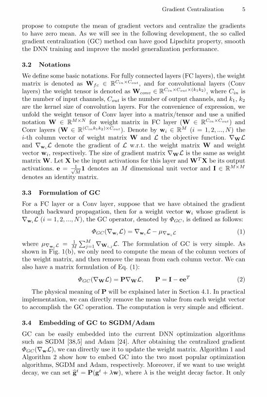
GC can be easily embedded into the current DNN optimization algorithmssuch as SGDM [38,5] and Adam [24]. After obtaining the centralized gradientΦGC(∇wL), we can directly use it to update the weight matrix. Algorithm 1 andAlgorithm 2 show how to embed GC into the two most popular optimizationalgorithms, SGDM and Adam, respectively. Moreover, if we want to use weightdecay, we can set gt = P(gt + λw), where λ is the weight decay factor. It only

6 H. Yong et al.

needs to add one line of code into most existing DNN optimization algorithmsto execute GC with negligible additional computational cost. For example, itcosts only 0.6 sec extra training time in one epoch on CIFAR100 with ResNet50model in our experiments (71 sec for one epoch).

Algorithm 1 SGDM with Gradient Centralization

Input: Weight vector w0, step size α, mo-mentum factor β, m0

Training step:1: for t = 1, ...T do2: gt = ∇wtL

3: gt = ΦGC(gt)4: mt = βmt−1 + (1− β)gt

5: wt+1 = wt − αmt

6: end for

Algorithm 2 Adam with Gradient Centralization

Input: Weight vector w0, step size α, β1,β2, ε, m0,v0

Training step:1: for t = 1, ...T do2: gt = ∇wtL3: gt = ΦGC(gt)

4: mt = β1mt−1 + (1− β1)gt

5: vt = β2vt−1 + (1− β2)gt � gt

6: mt = mt/(1− (β1)t)7: vt = vt/(1− (β2)t)

8: wt+1 = wt − α mt√vt+ε

9: end for

4 Properties of GC

As we will see in the section of experimental result, GC can accelerate the train-ing process and improve the generalization performance of DNNs. In this section,we perform theoretical analysis to explain why GC works.

4.1 Improving Generalization Performance

One important advantage of GC is that it can improve the generalization per-formance of DNNs. We explain this advantage from two aspects: weight spaceregularization and output feature space regularization.

Weight space regularization: Let’s first explain the physical meaning ofP in Eq.(2). Actually, it is easy to prove that:

P2 = P = PT , eTP∇WL = 0. (3)

The above equations show that P is the projection matrix for the hyperplanewith normal vector e in weight space, and P∇WL is the projected gradient.

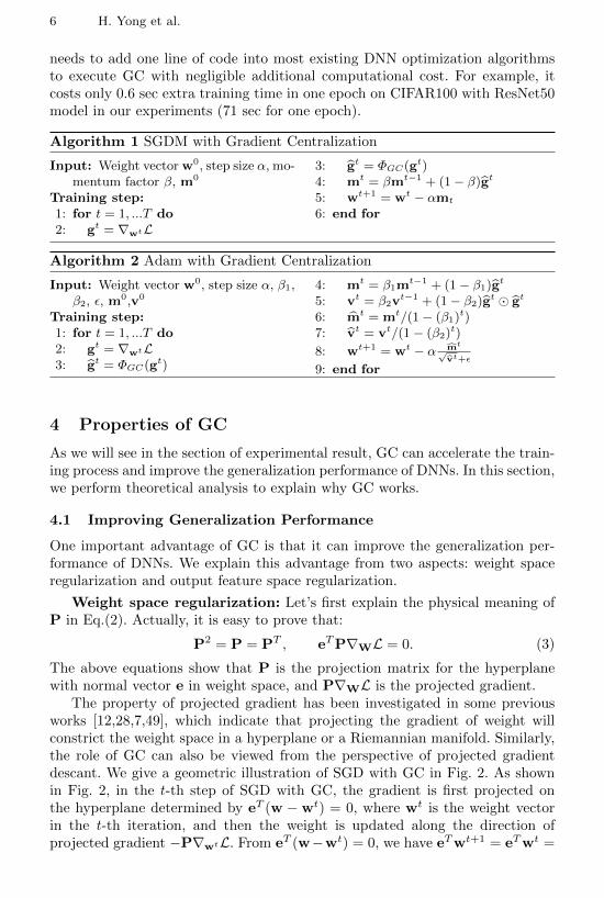
The property of projected gradient has been investigated in some previousworks [12,28,7,49], which indicate that projecting the gradient of weight willconstrict the weight space in a hyperplane or a Riemannian manifold. Similarly,the role of GC can also be viewed from the perspective of projected gradientdescant. We give a geometric illustration of SGD with GC in Fig. 2. As shownin Fig. 2, in the t-th step of SGD with GC, the gradient is first projected onthe hyperplane determined by eT (w − wt) = 0, where wt is the weight vectorin the t-th iteration, and then the weight is updated along the direction ofprojected gradient −P∇wtL. From eT (w−wt) = 0, we have eTwt+1 = eTwt =

Gradient Centralization 7

Fig. 2. The geometrical interpretation of GC. The gradient is projected on a hyperplaneeT (w −wt) = 0, where the projected gradient is used to update the weight.

... = eTw0, i.e., eTw is a constant during training. Mathematically, the latentobjective function w.r.t. one weight vector w can be written as follows:

minwL(w), s.t. eT (w −w0) = 0 (4)

Clearly, this is a constrained optimization problem on weight vector w. It regu-larizes the solution space of w, reducing the possibility of over-fitting on trainingdata. As a result, GC can improve the generalization capability of trained DNNmodels, especially when the number of training samples is limited.

It is noted that WS [39] uses a constraint eTw = 0 for weight optimization. Itreparameterizes weights to meet this constraint. However, this constraint largelylimits its practical applications because the initialized weight may not satisfythis constraint. For example, a pretrained DNN on ImageNet usually cannotmeet eTw0 = 0 for its initialized weight vectors. If we use WS to fine-tunethis DNN, the advantages of pretrained models will disappear. Therefore, wehave to retrain the DNN on ImageNet with WS before we fine-tune it. Thisis very cumbersome. Fortunately the weight constraint of GC in Eq. (4) fitsany initialization of weight, e.g., ImageNet pretrained initialization, because itinvolves the initialized weight w0 into the constraint so that eT (w0 −w0) = 0is always true. This greatly extends the applications of GC.

Output feature space regularization: For SGD based algorithms, wehave wt+1 = wt−αtP∇wtL. It can be derived that wt = w0−P

∑t−1i=0 α

(i)∇w(i)L.For any input feature vector x, we have the following theorem:

Theorem 4.1: Suppose that SGD (or SGDM) with GC is used to update theweight vector w, for any input feature vectors x and x + γ1, we have

(wt)Tx− (wt)T (x + γ1) = γ1Tw0 (5)

where w0 is the initial weight vector and γ is a scalar.

Please find the proof in the Appendix. Theorem 4.1 indicates that a con-stant intensity change (i.e., γ1) of an input feature causes a change of outputactivation; interestingly, this change is only related to γ and 1Tw0 but not thecurrent weight vector wt. 1Tw0 is the scaled mean of the initial weight vectorw0. In particular, if the mean of w0 is close to zero, then the output activationis not sensitive to the intensity change of input features, and the output featurespace becomes more robust to training sample variations.

8 H. Yong et al.

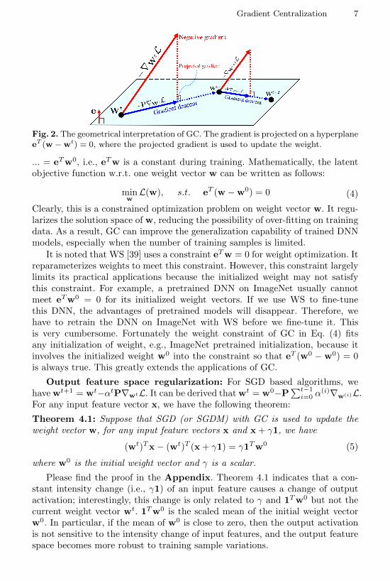
Fig. 3. The absolute value (log scale) of the mean of weight vectors for convolutionlayers in ResNet50. The x-axis is the weight vector index. We plot the mean value ofdifferent convolution layers from left to right with the order from sallow to deep layers.Kaiming normal initialization [14] (top) and ImageNet pre-trained weight initialization(bottom) are employed here. We can see that the mean values are usually very small(less than e−7) for most of the weight vectors.

Indeed, the mean of w0 is very close to zero by the commonly used weight ini-tialization strategies, such as Xavier initialization [11], Kaiming initialization [14]and even ImageNet pre-trained weight initialization. Fig. 3 shows the absolutevalue (log scale) of the mean of weight vectors for Conv layers in ResNet50 withKaiming normal initialization and ImageNet pre-trained weight initialization.We can see that the mean values of most weight vectors are very small and closeto zero (less than e−7). This ensures that if we train the DNN model with GC,the output features will not be sensitive to the variation of the intensity of in-put features. This property regularizes the output feature space and boosts thegeneralization performance of DNN training.

4.2 Accelerating Training Process

Optimization landscape smoothing: It has been shown in [45,39] that bothBN and WS smooth the optimization landscape. Although BN and WS oper-ate on activations and weights, they implicitly constrict the gradient of weights,making the gradient of weight more predictive and stable for fast training. Specif-ically, BN and WS use the gradient magnitude ||∇f(x)||2 to capture the Lip-schitzness of function f(x). For the loss and its gradients, f(x) will be L and∇wL, respectively, and x will be w. The upper bounds of ||∇wL||2 and ||∇2

wL||2(∇2

wL is the Hessian matrix of w) have been given in [45,39] to illustrate theoptimization landscape smoothing property of BN and WS. Similar conclusioncan be made for our proposed GC by comparing the Lipschitzness of original lossfunction L(w) with the constrained loss function in Eq. (4) and the Lipschitznessof their gradients. We have the following theorem:Theorem 4.2: Suppose ∇wL is the gradient of loss function L w.r.t. weight vec-tor w. With the ΦGC(∇wL) defined in Eq.(2), we have the following conclusionfor the loss function and its gradient, respectively:{

||ΦGC(∇wL)||2 ≤ ||∇wL||2,||∇wΦGC(∇wL)||2 ≤ ||∇2

wL||2.(6)

Gradient Centralization 9

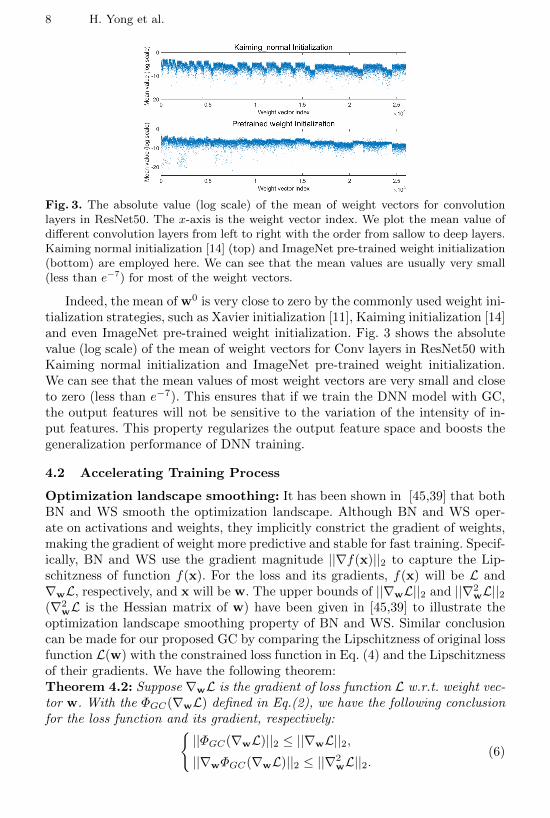
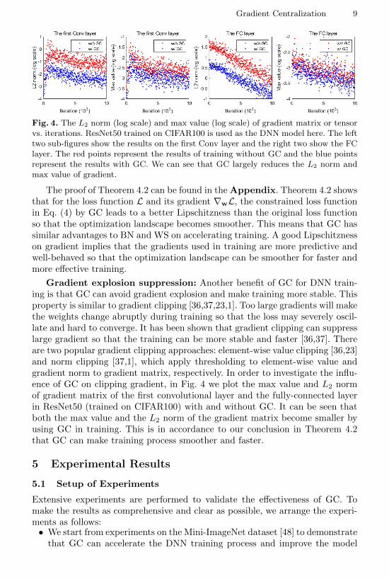
Fig. 4. The L2 norm (log scale) and max value (log scale) of gradient matrix or tensorvs. iterations. ResNet50 trained on CIFAR100 is used as the DNN model here. The lefttwo sub-figures show the results on the first Conv layer and the right two show the FClayer. The red points represent the results of training without GC and the blue pointsrepresent the results with GC. We can see that GC largely reduces the L2 norm andmax value of gradient.

The proof of Theorem 4.2 can be found in the Appendix. Theorem 4.2 showsthat for the loss function L and its gradient ∇wL, the constrained loss functionin Eq. (4) by GC leads to a better Lipschitzness than the original loss functionso that the optimization landscape becomes smoother. This means that GC hassimilar advantages to BN and WS on accelerating training. A good Lipschitznesson gradient implies that the gradients used in training are more predictive andwell-behaved so that the optimization landscape can be smoother for faster andmore effective training.

Gradient explosion suppression: Another benefit of GC for DNN train-ing is that GC can avoid gradient explosion and make training more stable. Thisproperty is similar to gradient clipping [36,37,23,1]. Too large gradients will makethe weights change abruptly during training so that the loss may severely oscil-late and hard to converge. It has been shown that gradient clipping can suppresslarge gradient so that the training can be more stable and faster [36,37]. Thereare two popular gradient clipping approaches: element-wise value clipping [36,23]and norm clipping [37,1], which apply thresholding to element-wise value andgradient norm to gradient matrix, respectively. In order to investigate the influ-ence of GC on clipping gradient, in Fig. 4 we plot the max value and L2 normof gradient matrix of the first convolutional layer and the fully-connected layerin ResNet50 (trained on CIFAR100) with and without GC. It can be seen thatboth the max value and the L2 norm of the gradient matrix become smaller byusing GC in training. This is in accordance to our conclusion in Theorem 4.2that GC can make training process smoother and faster.

5 Experimental Results

5.1 Setup of Experiments

Extensive experiments are performed to validate the effectiveness of GC. Tomake the results as comprehensive and clear as possible, we arrange the experi-ments as follows:• We start from experiments on the Mini-ImageNet dataset [48] to demonstrate

that GC can accelerate the DNN training process and improve the model

10 H. Yong et al.

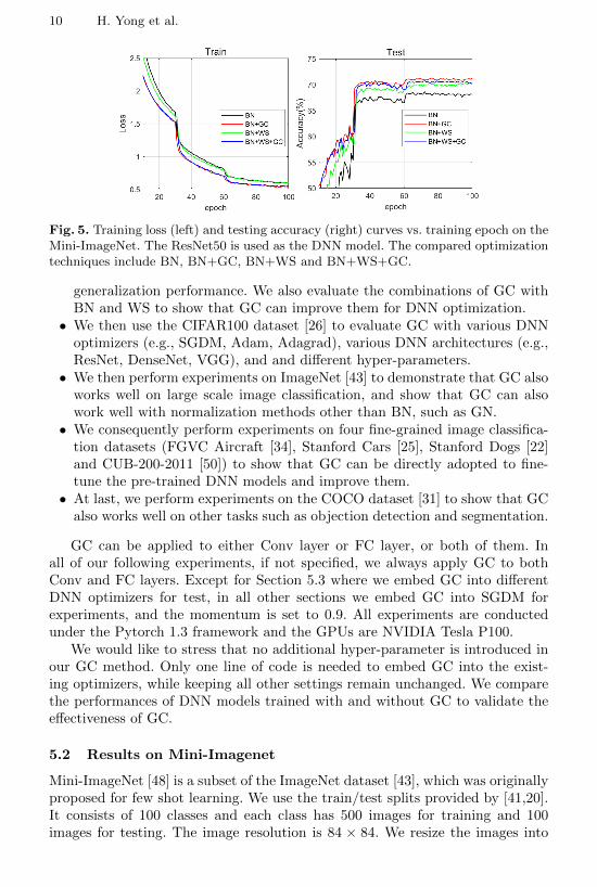
Fig. 5. Training loss (left) and testing accuracy (right) curves vs. training epoch on theMini-ImageNet. The ResNet50 is used as the DNN model. The compared optimizationtechniques include BN, BN+GC, BN+WS and BN+WS+GC.

generalization performance. We also evaluate the combinations of GC withBN and WS to show that GC can improve them for DNN optimization.• We then use the CIFAR100 dataset [26] to evaluate GC with various DNN

optimizers (e.g., SGDM, Adam, Adagrad), various DNN architectures (e.g.,ResNet, DenseNet, VGG), and and different hyper-parameters.• We then perform experiments on ImageNet [43] to demonstrate that GC also

works well on large scale image classification, and show that GC can alsowork well with normalization methods other than BN, such as GN.• We consequently perform experiments on four fine-grained image classifica-

tion datasets (FGVC Aircraft [34], Stanford Cars [25], Stanford Dogs [22]and CUB-200-2011 [50]) to show that GC can be directly adopted to fine-tune the pre-trained DNN models and improve them.• At last, we perform experiments on the COCO dataset [31] to show that GC

also works well on other tasks such as objection detection and segmentation.

GC can be applied to either Conv layer or FC layer, or both of them. Inall of our following experiments, if not specified, we always apply GC to bothConv and FC layers. Except for Section 5.3 where we embed GC into differentDNN optimizers for test, in all other sections we embed GC into SGDM forexperiments, and the momentum is set to 0.9. All experiments are conductedunder the Pytorch 1.3 framework and the GPUs are NVIDIA Tesla P100.

We would like to stress that no additional hyper-parameter is introduced inour GC method. Only one line of code is needed to embed GC into the exist-ing optimizers, while keeping all other settings remain unchanged. We comparethe performances of DNN models trained with and without GC to validate theeffectiveness of GC.

5.2 Results on Mini-Imagenet

Mini-ImageNet [48] is a subset of the ImageNet dataset [43], which was originallyproposed for few shot learning. We use the train/test splits provided by [41,20].It consists of 100 classes and each class has 500 images for training and 100images for testing. The image resolution is 84 × 84. We resize the images into

Gradient Centralization 11

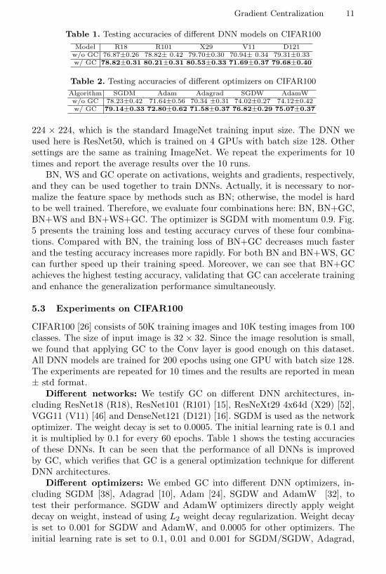
Table 1. Testing accuracies of different DNN models on CIFAR100

Model R18 R101 X29 V11 D121w/o GC 76.87±0.26 78.82± 0.42 79.70±0.30 70.94± 0.34 79.31±0.33w/ GC 78.82±0.31 80.21±0.31 80.53±0.33 71.69±0.37 79.68±0.40

Table 2. Testing accuracies of different optimizers on CIFAR100

Algorithm SGDM Adam Adagrad SGDW AdamWw/o GC 78.23±0.42 71.64±0.56 70.34 ±0.31 74.02±0.27 74.12±0.42w/ GC 79.14±0.33 72.80±0.62 71.58±0.37 76.82±0.29 75.07±0.37

224 × 224, which is the standard ImageNet training input size. The DNN weused here is ResNet50, which is trained on 4 GPUs with batch size 128. Othersettings are the same as training ImageNet. We repeat the experiments for 10times and report the average results over the 10 runs.

BN, WS and GC operate on activations, weights and gradients, respectively,and they can be used together to train DNNs. Actually, it is necessary to nor-malize the feature space by methods such as BN; otherwise, the model is hardto be well trained. Therefore, we evaluate four combinations here: BN, BN+GC,BN+WS and BN+WS+GC. The optimizer is SGDM with momentum 0.9. Fig.5 presents the training loss and testing accuracy curves of these four combina-tions. Compared with BN, the training loss of BN+GC decreases much fasterand the testing accuracy increases more rapidly. For both BN and BN+WS, GCcan further speed up their training speed. Moreover, we can see that BN+GCachieves the highest testing accuracy, validating that GC can accelerate trainingand enhance the generalization performance simultaneously.

5.3 Experiments on CIFAR100

CIFAR100 [26] consists of 50K training images and 10K testing images from 100classes. The size of input image is 32 × 32. Since the image resolution is small,we found that applying GC to the Conv layer is good enough on this dataset.All DNN models are trained for 200 epochs using one GPU with batch size 128.The experiments are repeated for 10 times and the results are reported in mean± std format.

Different networks: We testify GC on different DNN architectures, in-cluding ResNet18 (R18), ResNet101 (R101) [15], ResNeXt29 4x64d (X29) [52],VGG11 (V11) [46] and DenseNet121 (D121) [16]. SGDM is used as the networkoptimizer. The weight decay is set to 0.0005. The initial learning rate is 0.1 andit is multiplied by 0.1 for every 60 epochs. Table 1 shows the testing accuraciesof these DNNs. It can be seen that the performance of all DNNs is improvedby GC, which verifies that GC is a general optimization technique for differentDNN architectures.

Different optimizers: We embed GC into different DNN optimizers, in-cluding SGDM [38], Adagrad [10], Adam [24], SGDW and AdamW [32], totest their performance. SGDW and AdamW optimizers directly apply weightdecay on weight, instead of using L2 weight decay regularization. Weight decayis set to 0.001 for SGDW and AdamW, and 0.0005 for other optimizers. Theinitial learning rate is set to 0.1, 0.01 and 0.001 for SGDM/SGDW, Adagrad,

12 H. Yong et al.

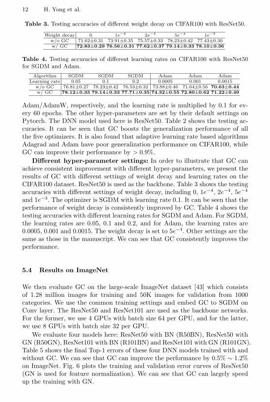
Table 3. Testing accuracies of different weight decay on CIFAR100 with ResNet50.

Weight decay 0 1e−4 2e−4 5e−4 1e−3

w/o GC 71.62±0.31 73.91±0.35 75.57±0.33 78.23±0.42 77.43±0.30w/ GC 72.83±0.29 76.56±0.31 77.62±0.37 79.14±0.33 78.10±0.36

Table 4. Testing accuracies of different learning rates on CIFAR100 with ResNet50for SGDM and Adam.

Algorithm SGDM SGDM SGDM Adam Adam AdamLearning rate 0.05 0.1 0.2 0.0005 0.001 0.0015

w/o GC 76.81±0.27 78.23±0.42 76.53±0.32 73.88±0.46 71.64±0.56 70.63±0.44w/ GC 78.12±0.33 79.14±0.33 77.71±0.35 74.32±0.55 72.80±0.62 71.22±0.49

Adam/AdamW, respectively, and the learning rate is multiplied by 0.1 for ev-ery 60 epochs. The other hyper-parameters are set by their default settings onPytorch. The DNN model used here is ResNet50. Table 2 shows the testing ac-curacies. It can be seen that GC boosts the generalization performance of allthe five optimizers. It is also found that adaptive learning rate based algorithmsAdagrad and Adam have poor generalization performance on CIFAR100, whileGC can improve their performance by > 0.9%.

Different hyper-parameter settings: In order to illustrate that GC canachieve consistent improvement with different hyper-parameters, we present theresults of GC with different settings of weight decay and learning rates on theCIFAR100 dataset. ResNet50 is used as the backbone. Table 3 shows the testingaccuracies with different settings of weight decay, including 0, 1e−4, 2e−4, 5e−4

and 1e−3. The optimizer is SGDM with learning rate 0.1. It can be seen that theperformance of weight decay is consistently improved by GC. Table 4 shows thetesting accuracies with different learning rates for SGDM and Adam. For SGDM,the learning rates are 0.05, 0.1 and 0.2, and for Adam, the learning rates are0.0005, 0.001 and 0.0015. The weight decay is set to 5e−4. Other settings are thesame as those in the manuscript. We can see that GC consistently improves theperformance.

5.4 Results on ImageNet

We then evaluate GC on the large-scale ImageNet dataset [43] which consistsof 1.28 million images for training and 50K images for validation from 1000categories. We use the common training settings and embed GC to SGDM onConv layer. The ResNet50 and ResNet101 are used as the backbone networks.For the former, we use 4 GPUs with batch size 64 per GPU, and for the latter,we use 8 GPUs with batch size 32 per GPU.

We evaluate four models here: ResNet50 with BN (R50BN), ResNet50 withGN (R50GN), ResNet101 with BN (R101BN) and ResNet101 with GN (R101GN).Table 5 shows the final Top-1 errors of these four DNN models trained with andwithout GC. We can see that GC can improve the performance by 0.5% ∼ 1.2%on ImageNet. Fig. 6 plots the training and validation error curves of ResNet50(GN is used for feature normalization). We can see that GC can largely speedup the training with GN.

Gradient Centralization 13

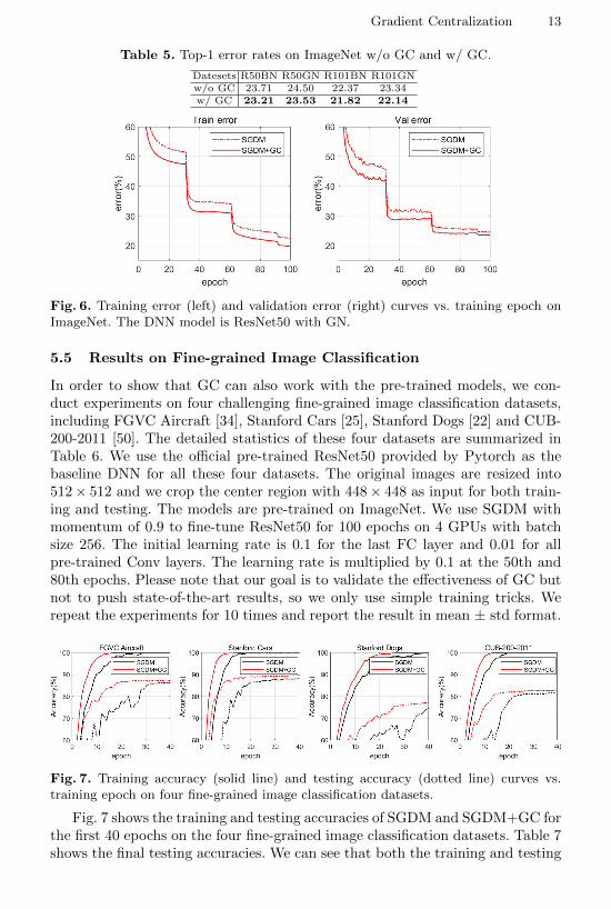
Table 5. Top-1 error rates on ImageNet w/o GC and w/ GC.

Datesets R50BN R50GN R101BN R101GNw/o GC 23.71 24.50 22.37 23.34w/ GC 23.21 23.53 21.82 22.14

Fig. 6. Training error (left) and validation error (right) curves vs. training epoch onImageNet. The DNN model is ResNet50 with GN.

5.5 Results on Fine-grained Image Classification

In order to show that GC can also work with the pre-trained models, we con-duct experiments on four challenging fine-grained image classification datasets,including FGVC Aircraft [34], Stanford Cars [25], Stanford Dogs [22] and CUB-200-2011 [50]. The detailed statistics of these four datasets are summarized inTable 6. We use the official pre-trained ResNet50 provided by Pytorch as thebaseline DNN for all these four datasets. The original images are resized into512× 512 and we crop the center region with 448× 448 as input for both train-ing and testing. The models are pre-trained on ImageNet. We use SGDM withmomentum of 0.9 to fine-tune ResNet50 for 100 epochs on 4 GPUs with batchsize 256. The initial learning rate is 0.1 for the last FC layer and 0.01 for allpre-trained Conv layers. The learning rate is multiplied by 0.1 at the 50th and80th epochs. Please note that our goal is to validate the effectiveness of GC butnot to push state-of-the-art results, so we only use simple training tricks. Werepeat the experiments for 10 times and report the result in mean ± std format.

Fig. 7. Training accuracy (solid line) and testing accuracy (dotted line) curves vs.training epoch on four fine-grained image classification datasets.

Fig. 7 shows the training and testing accuracies of SGDM and SGDM+GC forthe first 40 epochs on the four fine-grained image classification datasets. Table 7shows the final testing accuracies. We can see that both the training and testing

14 H. Yong et al.

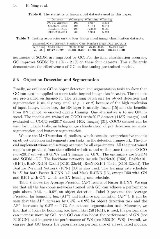
Table 6. The statistics of fine-grained datasets used in this paper.

Datasets #Category #Training #TestingFGVC Aircraft 100 6,667 3,333Stanford Cars 196 8,144 8,041Stanford Dogs 120 12,000 8,580CUB-200-2011 200 5,994 5,794

Table 7. Testing accuracies on the four fine-grained image classification datasets.

Datesets FGVC Aircraft Stanford Cars Stanford Dogs CUB-200-2011w/o GC 86.62±0.31 88.66±0.22 76.16±0.25 82.07±0.26w/ GC 87.77±0.27 90.03±0.26 78.23±0.24 83.40±0.30

accuracies of SGDM are improved by GC. For the final classification accuracy,GC improves SGDM by 1.1% ∼ 2.1% on these four datasets. This sufficientlydemonstrates the effectiveness of GC on fine-tuning pre-trained models.

5.6 Objection Detection and Segmentation

Finally, we evaluate GC on object detection and segmentation tasks to show thatGC can also be applied to more tasks beyond image classification. The modelsare pre-trained on ImageNet. The training batch size for object detection andsegmentation is usually very small (e.g., 1 or 2) because of the high resolutionof input image. Therefore, the BN layer is usually frozen [15] and the benefitsfrom BN cannot be enjoyed during training. One alternative is to use GN in-stead. The models are trained on COCO train2017 dataset (118K images) andevaluated on COCO val2017 dataset (40K images) [31]. COCO dataset can beused for multiple tasks, including image classification, object detection, semanticsegmentation and instance segmentation.

We use the MMDetection [6] toolbox, which contains comprehensive modelson object detection and segmentation tasks, as the detection framework. The offi-cial implementations and settings are used for all experiments. All the pre-trainedmodels are provided from their official websites, and we fine-tune them on COCOtrain2017 set with 8 GPUs and 2 images per GPU. The optimizers are SGDMand SGDM+GC. The backbone networks include ResNet50 (R50), ResNet101(R101), ResNeXt101-32x4d (X101-32x4d), ResNeXt101-64x4d (X101-32x4d). TheFeature Pyramid Network (FPN) [30] is also used. The learning rate scheduleis 1X for both Faster R-CNN [42] and Mask R-CNN [13], except R50 with GNand R101 with GN, which use 2X learning rate schedule.

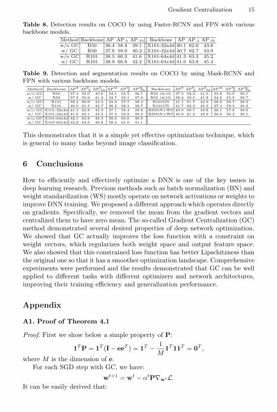
Tabel 8 shows the Average Precision (AP) results of Faster R-CNN. We cansee that all the backbone networks trained with GC can achieve a performancegain about 0.3% ∼ 0.6% on object detection. Tabel 9 presents the AveragePrecision for bounding box (APb) and instance segmentation (APm). It can beseen that the APb increases by 0.5% ∼ 0.9% for object detection task and theAPm increases by 0.3% ∼ 0.7% for instance segmentation task. Moreover, wefind that if 4conv1fc bounding box head, like R50 (4c1f), is used, the performancecan increase more by GC. And GC can also boost the performance of GN (seeR101GN) and improve the performance of WS (see R50GN+WS). Overall, wecan see that GC boosts the generalization performance of all evaluated models.

Gradient Centralization 15

Table 8. Detection results on COCO by using Faster-RCNN and FPN with variousbackbone models.

Method Backbone AP AP.5 AP.75 Backbone AP AP.5 AP.75

w/o GC R50 36.4 58.4 39.1 X101-32x4d 40.1 62.0 43.8w/ GC R50 37.0 59.0 40.2 X101-32x4d 40.7 62.7 43.9w/o GC R101 38.5 60.3 41.6 X101-64x4d 41.3 63.3 45.2w/ GC R101 38.9 60.8 42.2 X101-64x4d 41.6 63.8 45.4

Table 9. Detection and segmentation results on COCO by using Mask-RCNN andFPN with various backbone models.

Method Backbone APb APb.5 APb

.75 APm APm.5 APm

.75 Backbone APb APb.5 APb

.75 APm APm.5 APm

.75w/o GC R50 37.4 59.0 40.6 34.1 55.5 36.1 R50 (4c1f) 37.5 58.2 41.0 33.9 55.0 36.1w/ GC R50 37.9 59.6 41.2 34.7 56.1 37.0 R50 (4c1f) 38.4 59.5 41.8 34.6 55.9 36.7

w/o GC R101 39.4 60.9 43.3 35.9 57.7 38.4 R101GN 41.1 61.7 44.9 36.9 58.7 39.3w/ GC R101 40.0 61.5 43.7 36.2 58.1 38.7 R101GN 41.7 62.3 45.3 37.4 59.3 40.3

w/o GC X101-32x4d 41.1 62.8 45.0 37.1 59.4 39.8 R50GN+WS 40.0 60.7 43.6 36.1 57.8 38.6w/ GC X101-32x4d 41.6 63.1 45.5 37.4 59.8 39.9 R50GN+WS 40.6 61.3 43.9 36.6 58.2 39.1

w/o GC X101-64x4d 42.1 63.8 46.3 38.0 60.6 40.9w/ GC X101-64x4d 42.8 64.5 46.8 38.4 61.0 41.1

This demonstrates that it is a simple yet effective optimization technique, whichis general to many tasks beyond image classification.

6 Conclusions

How to efficiently and effectively optimize a DNN is one of the key issues indeep learning research. Previous methods such as batch normalization (BN) andweight standardization (WS) mostly operate on network activations or weights toimprove DNN training. We proposed a different approach which operates directlyon gradients. Specifically, we removed the mean from the gradient vectors andcentralized them to have zero mean. The so-called Gradient Centralization (GC)method demonstrated several desired properties of deep network optimization.We showed that GC actually improves the loss function with a constraint onweight vectors, which regularizes both weight space and output feature space.We also showed that this constrained loss function has better Lipschitzness thanthe original one so that it has a smoother optimization landscape. Comprehensiveexperiments were performed and the results demonstrated that GC can be wellapplied to different tasks with different optimizers and network architectures,improving their training efficiency and generalization performance.

Appendix

A1. Proof of Theorem 4.1

Proof. First we show below a simple property of P:

1TP = 1T (I− eeT ) = 1T − 1

M1T11T = 0T ,

where M is the dimension of e.For each SGD step with GC, we have:

wt+1 = wt − αtP∇wtL.It can be easily derived that:

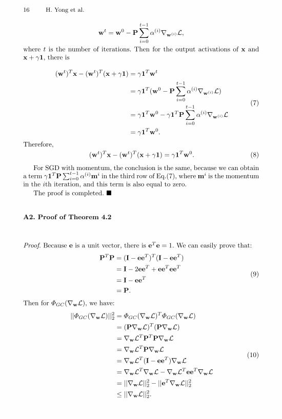
16 H. Yong et al.

wt = w0 −P

t−1∑i=0

α(i)∇w(i)L,

where t is the number of iterations. Then for the output activations of x andx + γ1, there is

(wt)Tx− (wt)T (x + γ1) = γ1Twt

= γ1T (w0 −P

t−1∑i=0

α(i)∇w(i)L)

= γ1Tw0 − γ1TP

t−1∑i=0

α(i)∇w(i)L

= γ1Tw0.

(7)

Therefore,

(wt)Tx− (wt)T (x + γ1) = γ1Tw0. (8)

For SGD with momentum, the conclusion is the same, because we can obtaina term γ1TP

∑t−1i=0 α

(i)mi in the third row of Eq.(7), where mi is the momentumin the ith iteration, and this term is also equal to zero.

The proof is completed. �

A2. Proof of Theorem 4.2

Proof. Because e is a unit vector, there is eTe = 1. We can easily prove that:

PTP = (I− eeT )T (I− eeT )

= I− 2eeT + eeTeeT

= I− eeT

= P.

(9)

Then for ΦGC(∇wL), we have:

||ΦGC(∇wL)||22 = ΦGC(∇wL)TΦGC(∇wL)

= (P∇wL)T (P∇wL)

= ∇wLTPTP∇wL= ∇wLTP∇wL= ∇wLT (I− eeT )∇wL= ∇wLT∇wL −∇wLTeeT∇wL= ||∇wL||22 − ||eT∇wL||22≤ ||∇wL||22.

(10)

Gradient Centralization 17

For ∇wΦGC(∇wL), we also have

||∇ΦGC(∇wL)||22 = ||P∇2wL||22

= ∇2wLTPTP∇2

wL= ∇2

wLTP∇2wL

= ||∇2wL||22 − ||eT∇2

wL||22≤ ||∇2

wL||22.

(11)

The proof is completed. �

18 H. Yong et al.

References

1. Abadi, M., Chu, A., Goodfellow, I., McMahan, H.B., Mironov, I., Talwar, K.,Zhang, L.: Deep learning with differential privacy. In: Proceedings of the 2016ACM SIGSAC Conference on Computer and Communications Security. pp. 308–318. ACM (2016)

2. Abu-El-Haija, S., Kothari, N., Lee, J., Natsev, P., Toderici, G., Varadarajan, B.,Vijayanarasimhan, S.: Youtube-8m: A large-scale video classification benchmark.arXiv preprint arXiv:1609.08675 (2016)

3. Bjorck, J., Gomes, C., Selman, B., Weinberger, K.Q.: Understanding batch nor-malization pp. 7694–7705 (2018)

4. Bottou, L.: Stochastic gradient learning in neural networks. Proceedings of Neuro-Nımes 91(8), 12 (1991)

5. Bottou, L.: Large-scale machine learning with stochastic gradient descent. In: Pro-ceedings of COMPSTAT’2010, pp. 177–186. Springer (2010)

6. Chen, K., Wang, J., Pang, J., Cao, Y., Xiong, Y., Li, X., Sun, S., Feng, W., Liu,Z., Xu, J., et al.: Mmdetection: Open mmlab detection toolbox and benchmark.arXiv preprint arXiv:1906.07155 (2019)

7. Cho, M., Lee, J.: Riemannian approach to batch normalization. In: Advances inNeural Information Processing Systems. pp. 5225–5235 (2017)

8. Courbariaux, M., Bengio, Y., David, J.P.: Binaryconnect: Training deep neural net-works with binary weights during propagations. In: Advances in neural informationprocessing systems. pp. 3123–3131 (2015)

9. Courbariaux, M., Hubara, I., Soudry, D., El-Yaniv, R., Bengio, Y.: Binarized neuralnetworks: Training deep neural networks with weights and activations constrainedto+ 1 or-1. arXiv preprint arXiv:1602.02830 (2016)

10. Duchi, J., Hazan, E., Singer, Y.: Adaptive subgradient methods for online learningand stochastic optimization. Journal of Machine Learning Research 12(Jul), 2121–2159 (2011)

11. Glorot, X., Bengio, Y.: Understanding the difficulty of training deep feedforwardneural networks. In: Proceedings of the thirteenth international conference on ar-tificial intelligence and statistics. pp. 249–256 (2010)

12. Gupta, H., Jin, K.H., Nguyen, H.Q., McCann, M.T., Unser, M.: Cnn-based pro-jected gradient descent for consistent ct image reconstruction. IEEE transactionson medical imaging 37(6), 1440–1453 (2018)

13. He, K., Gkioxari, G., Dollar, P., Girshick, R.: Mask r-cnn. In: Proceedings of theIEEE international conference on computer vision. pp. 2961–2969 (2017)

14. He, K., Zhang, X., Ren, S., Sun, J.: Delving deep into rectifiers: Surpassing human-level performance on imagenet classification. In: Proceedings of the IEEE interna-tional conference on computer vision. pp. 1026–1034 (2015)

15. He, K., Zhang, X., Ren, S., Sun, J.: Deep residual learning for image recognition. In:Proceedings of the IEEE conference on computer vision and pattern recognition.pp. 770–778 (2016)

16. Huang, G., Liu, Z., Van Der Maaten, L., Weinberger, K.Q.: Densely connectedconvolutional networks. In: Proceedings of the IEEE conference on computer visionand pattern recognition. pp. 4700–4708 (2017)

17. Huang, L., Liu, X., Liu, Y., Lang, B., Tao, D.: Centered weight normalization inaccelerating training of deep neural networks. In: Proceedings of the IEEE Inter-national Conference on Computer Vision. pp. 2803–2811 (2017)

Gradient Centralization 19

18. Huang, X., Belongie, S.: Arbitrary style transfer in real-time with adaptive instancenormalization. In: Proceedings of the IEEE International Conference on ComputerVision. pp. 1501–1510 (2017)

19. Ioffe, S., Szegedy, C.: Batch normalization: Accelerating deep network training byreducing internal covariate shift. arXiv preprint arXiv:1502.03167 (2015)

20. Iscen, A., Tolias, G., Avrithis, Y., Chum, O.: Label propagation for deep semi-supervised learning. In: Proceedings of the IEEE Conference on Computer Visionand Pattern Recognition. pp. 5070–5079 (2019)

21. Karpathy, A., Toderici, G., Shetty, S., Leung, T., Sukthankar, R., Fei-Fei, L.: Large-scale video classification with convolutional neural networks. In: Proceedings ofthe IEEE conference on Computer Vision and Pattern Recognition. pp. 1725–1732(2014)

22. Khosla, A., Jayadevaprakash, N., Yao, B., Li, F.F.: Novel dataset for fgvc: Stanforddogs. In: San Diego: CVPR Workshop on FGVC. vol. 1 (2011)

23. Kim, J., Kwon Lee, J., Mu Lee, K.: Accurate image super-resolution using verydeep convolutional networks. In: Proceedings of the IEEE conference on computervision and pattern recognition. pp. 1646–1654 (2016)

24. Kingma, D.P., Ba, J.: Adam: A method for stochastic optimization. arXiv preprintarXiv:1412.6980 (2014)

25. Krause, J., Stark, M., Deng, J., Fei-Fei, L.: 3d object representations for fine-grained categorization. In: Proceedings of the IEEE International Conference onComputer Vision Workshops. pp. 554–561 (2013)

26. Krizhevsky, A., Hinton, G., et al.: Learning multiple layers of features from tinyimages. Tech. rep., Citeseer (2009)

27. Krogh, A., Hertz, J.A.: A simple weight decay can improve generalization. In:Advances in neural information processing systems. pp. 950–957 (1992)

28. Larsson, M., Arnab, A., Kahl, F., Zheng, S., Torr, P.: A projected gradient descentmethod for crf inference allowing end-to-end training of arbitrary pairwise poten-tials. In: International Workshop on Energy Minimization Methods in ComputerVision and Pattern Recognition. pp. 564–579. Springer (2017)

29. Lei Ba, J., Kiros, J.R., Hinton, G.E.: Layer normalization. arXiv preprintarXiv:1607.06450 (2016)

30. Lin, T.Y., Dollar, P., Girshick, R., He, K., Hariharan, B., Belongie, S.: Featurepyramid networks for object detection. In: Proceedings of the IEEE conference oncomputer vision and pattern recognition. pp. 2117–2125 (2017)

31. Lin, T.Y., Maire, M., Belongie, S., Hays, J., Perona, P., Ramanan, D., Dollar, P.,Zitnick, C.L.: Microsoft coco: Common objects in context. In: European conferenceon computer vision. pp. 740–755. Springer (2014)

32. Loshchilov, I., Hutter, F.: Decoupled weight decay regularization. arXiv preprintarXiv:1711.05101 (2017)

33. Luo, P., Wang, X., Shao, W., Peng, Z.: Towards understanding regularization inbatch normalization (2018)

34. Maji, S., Rahtu, E., Kannala, J., Blaschko, M., Vedaldi, A.: Fine-grained visualclassification of aircraft. arXiv preprint arXiv:1306.5151 (2013)

35. Nair, V., Hinton, G.E.: Rectified linear units improve restricted boltzmann ma-chines. In: Proceedings of the 27th international conference on machine learning(ICML-10). pp. 807–814 (2010)

36. Pascanu, R., Mikolov, T., Bengio, Y.: Understanding the exploding gradient prob-lem. CoRR, abs/1211.5063 2 (2012)

37. Pascanu, R., Mikolov, T., Bengio, Y.: On the difficulty of training recurrent neuralnetworks. In: International conference on machine learning. pp. 1310–1318 (2013)

20 H. Yong et al.

38. Qian, N.: On the momentum term in gradient descent learning algorithms. Neuralnetworks 12(1), 145–151 (1999)

39. Qiao, S., Wang, H., Liu, C., Shen, W., Yuille, A.: Weight standardization. arXivpreprint arXiv:1903.10520 (2019)

40. Rastegari, M., Ordonez, V., Redmon, J., Farhadi, A.: Xnor-net: Imagenet classi-fication using binary convolutional neural networks. In: European Conference onComputer Vision. pp. 525–542. Springer (2016)

41. Ravi, S., Larochelle, H.: Optimization as a model for few-shot learning (2016)42. Ren, S., He, K., Girshick, R., Sun, J.: Faster r-cnn: Towards real-time object detec-

tion with region proposal networks. In: Advances in neural information processingsystems. pp. 91–99 (2015)

43. Russakovsky, O., Deng, J., Su, H., Krause, J., Satheesh, S., Ma, S., Huang, Z.,Karpathy, A., Khosla, A., Bernstein, M., et al.: Imagenet large scale visual recog-nition challenge. International journal of computer vision 115(3), 211–252 (2015)

44. Salimans, T., Kingma, D.P.: Weight normalization: A simple reparameterizationto accelerate training of deep neural networks. In: Advances in Neural InformationProcessing Systems. pp. 901–909 (2016)

45. Santurkar, S., Tsipras, D., Ilyas, A., Madry, A.: How does batch normalization helpoptimization? (no, it is not about internal covariate shift) pp. 2483–2493 (2018)

46. Simonyan, K., Zisserman, A.: Very deep convolutional networks for large-scaleimage recognition. arXiv preprint arXiv:1409.1556 (2014)

47. Ulyanov, D., Vedaldi, A., Lempitsky, V.: Instance normalization: The missing in-gredient for fast stylization. arXiv preprint arXiv:1607.08022 (2016)

48. Vinyals, O., Blundell, C., Lillicrap, T., Wierstra, D., et al.: Matching networksfor one shot learning. In: Advances in neural information processing systems. pp.3630–3638 (2016)

49. Vorontsov, E., Trabelsi, C., Kadoury, S., Pal, C.: On orthogonality and learningrecurrent networks with long term dependencies. In: Proceedings of the 34th Inter-national Conference on Machine Learning-Volume 70. pp. 3570–3578. JMLR. org(2017)

50. Wah, C., Branson, S., Welinder, P., Perona, P., Belongie, S.: The caltech-ucsdbirds-200-2011 dataset (2011)

51. Wu, Y., He, K.: Group normalization. In: Proceedings of the European Conferenceon Computer Vision (ECCV). pp. 3–19 (2018)

52. Xie, S., Girshick, R., Dollar, P., Tu, Z., He, K.: Aggregated residual transformationsfor deep neural networks. In: Proceedings of the IEEE conference on computervision and pattern recognition. pp. 1492–1500 (2017)

53. Zhang, C., Bengio, S., Hardt, M., Recht, B., Vinyals, O.: Understanding deeplearning requires rethinking generalization. arXiv preprint arXiv:1611.03530 (2016)

54. Zhang, G., Wang, C., Xu, B., Grosse, R.: Three mechanisms of weight decay reg-ularization. arXiv preprint arXiv:1810.12281 (2018)