Neural network approach to signal modelling in power systems

Neural network approach to signal modelling in power systems

K.L. Ting C.S. Berger M.F. Conlon

Indexing terms: Kohonen networks, Neural networks, Nonlinear modelling, Power transmission, VAR compensation

I I Abstract: A neural network approach to a system identification problem is presented. Traditional system identification techniques require knowledge of the model structure before parameter estimation methods can be applied. This approach requires less a priori information and the knowledge of model structure is not essential. A simulation study on a power system has demonstrated the application of this technique.

1 Introduction

Static VAR compensation (SVC) has been studied extens- ively in recent years. Recent research work mainly con- centrated on its application to enhance system transient stability and increase transmission capacity [l-41. Other power system applications of SVC includes voltage regu- lation and load compensation [ S , 61. Actual installation of SVCs in the power systems were also reported [6, 71.

The static VAR compensator is a reactive power device which can absorb or generate reactive power in the system when it is needed. One version of the SVC consists of a parallel combination of switched-capacitor banks and thyristor-controlled inductor banks. There are many different SVC configurations depending on the switching mechanism of the capacitor banks and the thyristor control of the firing angle. By controlling the switching of the capacitor banks and the firing angle of the thyristor, the reactance of the SVC can be varied from being fully capacitive to fully inductive. References 2, 7 and 8 discuss the configurations and characteristics of the SVC for power transmission system applications.

SVC controllers use two control signals, namely the local bus voltage to provide local voltage support and a stabilising signal to provide system damping. The stabilising signal is usually derived from an auxiliary variable which is local to the SVC bus, e.g. the local bus frequency, the line power flow, the speed or the acceler- ating power of the synchronous machine. The choice of the auxiliary signal will depend on the cause of oscillation. These local auxiliary variables may not be appropriate for some situations e.g. inter area oscillations and oscillations over a long transmission line, as they do not reflect the nature of the oscillations. Remote auxiliary

0 IEE, 1995 Paper l88lD (C8), first received 10th May 1994 and in revised form 13th February 1995 The authors are with the Department of Electrical and Computer Systems Engineering, Monash University, Clayton, Victoria, 3168, Australia

I E E Proc.-Control Theory Appl., Vol. 142, No. 4, July 1995

signals have been proposed for these situations, e.g. the computed internal frequency (CIF) [9] and the phase- angle difference between the oscillating areas [lo]. For practical purposes, these remote signals must be derived from the local measurable variables, e.g. the bus voltage, the active and reactive power flow. The techniques described in References 9 and 10 rely on an equivalent representation between the SVC bus and the synchronous machine involved, which can be derived from the actual power system. The accuracy of the equivalent representation depends on the knowledge of the system parameters which are not known accurately in general. System identification approach using the black box model to relate the local measurements and the remote phase signals provides an alternative method which does not require the knowledge of the system parameters.

Conventional system identification approach involves the determination of an appropriate model structure and then an adaptive parameter estimation scheme is used to estimate the parameters. Many well established parameter estimation schemes exist that work well for linear models, e.g. least square estimator, maximum likelihood estimators and prediction error estimators [ll]. When nonlinear dynamics exist, most of these schemes however require the knowledge of the actual system model structure, which is either unknown or difficult to obtain. Neural networks provide an alternative approach to this nonlinear dynamic identification problem. A neural network is a highly interconnected nonlinear system which can be considered as a nonlinear mapping between the input and the output. The use of multilayer feedforward networks and single-layer recurrent networks in nonlinear dynamic system identification with unknown structure is discussed in References 12 and 13.

In this paper, a neural network approach is presented which can model nonlinear functions and does not require the knowledge of the actual model structure. This approach only requires a set of input-output data for training. If the structure of the nonlinear dynamics is known, it can be used to improve the convergence of the parameter estimation. A simulation study on a power system with lCbus, four-machine and a SVC is used to show the superior performance of this neural network approach over the conventional system identification approach.

The authors are grateful to the Australian Elec- tricity Supply Industry Research Board for funding this project.

251

2 Neural networks

Neural networks have been applied successfully in different disciplines e.g. pattern recognition, robotic manipulator control and nonlinear function modelling [14, 201. Neural networks have also been applied to a variety of power system problems, e.g. static and dynamic stability assessment, load forecasting and fault identification. A three-layer feedforward network was proposed to calculate the critical fault-clearing time in Reference 15. Two stages of multilayer feedforward networks was proposed for the real-time control of multitap capacitors installed on a distribution system [16]. A single-layer Kohonen network was proposed for the power system conditions classifier [17, 181. A three-layer counter propagation network was proposed to identify the types of fault occurred during a disturbance [19].

A neural network basically consists of a set of weights which are trained during the learning phase until the model output matches the desired output. The rate of parameter convergence depends on the training data, the parameter adjustment algorithms and the network struc- tures. There are two main classes of neural networks, namely the multilayer feedforward network and the single-layer network. In multilayer networks, the weights are updated by the back-propagation algorithm where the error between the actual output of the network and the desired output is propagated back through all the layers and a gradient method is used to update the weights [12, 201. The training time is usually long because of the error back propagation and thus is not suitable for online training. On the other hand, there is no error propagation in the training of single-layer networks and thus the weights can adapt rapidly to cope with time-varying systems. Therefore single-layer networks are more suitable for control applications.

One of the well known single-layer networks is the Cerebellar model articulation controller (CMAC) origin- ally described by Albus [21]. It consists of a quantised multidimensional input space and an associative memory space. The weights stored in the associated memory are trained during the learning phase and can be updated during application, if necessary. The weights are used to interpolate the network output. One disadvantage of CMAC is its large memory requirement which is a function of the number of inputs and the quantisation inter- vals.

An improved version of CMAC called Cerebellar model with interpolation (CEINT) was proposed which has two improvements over standard CMAC, namely the adaptive partitioning of the input space and the network output as the multi-linear interpolation of the weights [22]. The CEINT has the capability to represent an equation error model. In this paper, the CEINT is modi- fied to handle the output error models by using the conjugate gradient weights opthisation algorithm [23]. The following Section describes CEINT and the modifications in detail and its application to system identification.

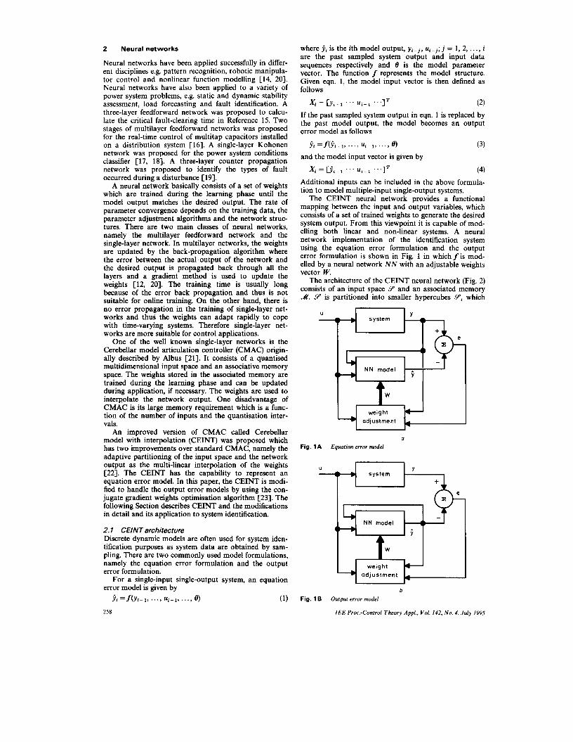
2.1 CEINT architecture Discrete dynamic models are often used for system identification purposes as system data are obtained by sampling. There are two commonly used model formulations, namely the equation error formulation and the output error formulation.

For a single-input single-output system, an equation error model is given by

ji =f(yi- . . . , ui- . . . , e) (1)

258

NN model 4- 9

where ji is the ith model output, y i - j , qj; j = 1, 2, . . . , i are the past sampled system output and input data sequences respectively and 0 is the model parameter vector. The function f represents the model structure. Given eqn. 1, the model input vector is then defined as follows

xi = r y - 1 ". " . I T (2) If the past sampled system output in eqn. 1 is replaced by the past model output, the model becomes an output error model as follows

ji = f(ji . . . , ui ~ . . . , e) (3)

xi = " ' ui-l . . . I T (4)

and the model input vector is given by

Additional inputs can be included in the above formulation to model multiple-input single-output systems.

The CEINT neural network provides a functional mapping between the input and output variables, which consists of a set of trained weights to generate the desired system output. From this viewpoint it is capable of modelling both linear and non-linear systems. A neural network implementation of the identification system using the equation error formulation and the output error formulation is shown in Fig. 1 in whichfis modelled by a neural network N N with an adjustable weights vector W.

The architecture of the CEINT neural network (Fig. 2) consists of an input space Y and an associated memory A. Y is partitioned into smaller hypercubes Yi which

t l N model 4-

Y

W

weight -

U

* adjustment -

a Fig. 1 A Equation error model

U _.

b

Fig. 1 B Output error model

I E E Prm.-Control Theory Appl., Vol. 142, N o . 4, July 1995

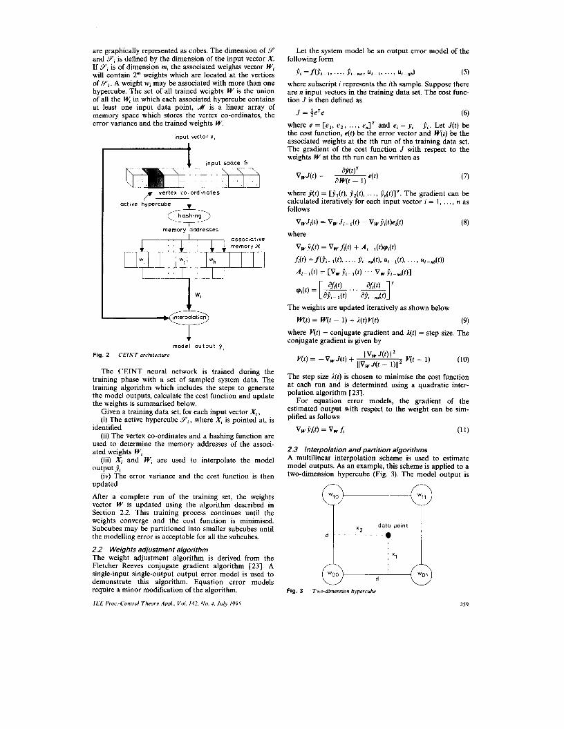
are graphically represented as cubes. The dimension of Y and Y i is defined by the dimension of the input vector X. If Y i is of dimension m, the associated weights vector Wi will contain 2" weights which are located at the vertices of Yi. A weight wi may be associated with more than one hypercube. The set of all trained weights W is the union of all the in which each associated hypercube contains at least one input data point, A is a linear array of memory space which stores the vertex co-ordinates, the error variance and the trained weights W.

Input vector x ,

I input space S

,y I vertex co:ordinotes

actwe hypercube 4 e memory 'addresses

74- associative

+ model output 9,

Fig. 2 C E I N T arrhitecfure

The CEINT neural network is trained during the training phase with a set of sampled system data. The training algorithm which includes the steps to generate the model outputs, calculate the cost function and update the weights is summarised below.

Given a training data set, for each input vector X i , (i) The active hypercube Y i , where Xi is pointed at, is

identified (ii) The vertex co-ordinates and a hashing function are

used to determine the memory addresses of the associated weights Wi

(iii) Xi and W, are used to interpolate the model

(iv) The error variance and the cost function is then updated

After a complete run of the training set, the weights vector W is updated using the algorithm described in Section 2.2. This training process continues until the weights converge and the cost function is minimised. Subcubes may be partitioned into smaller subcubes until the modelling error is acceptable for all the subcubes.

2.2 Weights adjustment algorithm The weight adjustment algorithm is derived from the Fletcher-Reeves conjugate gradient algorithm [23]. A single-input single-output output error model is used to demonstrate this algorithm. Equation error models require a minor modification of the algorithm.

output 9;

IEE Proc.-Control Theory Appl.. Vol. 142, N o . 4 . July 1995

Let the system model be an output error model of the following form

9 i = f ( j i - I , . . . , 9 i - . , , u i - l , . . . , U i - - n b ) ( 5 ) where subscript i represents the ith sample. Suppose there are n input vectors in the training data set. The cost function J is then defined as

J = f eTe (6) where e = [el, e2 , . . ., e,JT and ei = yi - j i . Let J(t) be the cost function, e(t) be the error vector and W(t) be the associated weights at the tth run of the training data set. The gradient of the cost function J with respect to the weights W at the tth run can be written as

a3(qT aW(t - 1) V,J(t) = - ~ 4t) (7)

The weights are updated iteratively as shown below

(9) W(t) = W(t - 1) + 4r )V( t ) where V(t) = conjugate gradient and l ( t ) = step size. The conjugate gradient is given by

The step size l ( t ) is chosen to minimise the cost function at each run and is determined using a quadratic interpolation algorithm [23 ] .

For equation error models, the gradient of the estimated output with respect to the weight can be simplified as follows

vw 9dt) = vw h (1 1)

2.3 Interpolation and partition algorithms A multilinear interpolation scheme is used to estimate model outputs. As an example, this scheme is applied to a two-dimension hypercube (Fig. 3). The model output is

. . . . . . . .

Fig. 3 Two-dimension hypercube

259

given by

j = woo(!+)(+) + wol(y)e) + Wl0(2) (+) + w,(?)(?) (12)

where wi are the weights and i = 0, 1, 2, 3 which are represented in binary format. For a m-dimensional hypercube, the interpolation becomes a summation of 2'" product terms as shown below

2 n - 1 n w . n If?.

$ = zo ( ;=l d )

(13) d - x j

x j

if jth bit of i(m-bit binary) = 0 ifjth bit of i(m-bit binary) = 1

k j = {

where

wi = weight at the ith vertex x j = distance from thejth dimension of the subspace d = length of the hypercube

This interpolation scheme has the following properties (a) weights are the functional values trained at the ver-

tices (b) interpolation along the boundary is only a function

of the vertices defining the boundary which ensures con- tinuity of the function across the hypercubes

(c) the product term is a m-linear function and thus an adequate nonlinear model may sometimes be attained without partitioning.

Higher order nonlinear dynamics can be modelled by further partitioning of the input space into smaller hypercubes. Bisection of a m-dimensional hypercube will create a set of new vertices and hypercubes and the maximum is V = (3" - 2") new vertices and S = 2" new hypercubes. Global partitioning of the whole input space will create a large number of new vertices and new hypercubes as V new vertices and S new hypercubes are created in each existing hypercube. Since only a subset of all the hypercubes will be entered, adaptive partitioning of the active hypercube reduces the number of new vertices and new hypercubes and thus the memory requirement. This localised partitioning scheme can adapt its memory requirement to the nonlinearity of the system dynamics.

The error variance associated with each active hypercube is chosen as an indication for further partition. The hypercube with the maximum error variance will be partitioned into finer hypercubes. The neural network training phase involves an iterative process of the weights adjustment and the adaptive partitioning of hypercubes until the cost function converges to the desired minimum.

3 Power system application

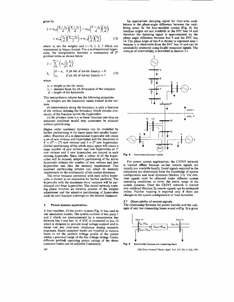
A four-machine, 1Cbus power system (Fig. 4) was used in our simulation studies. The system consists of two areas 1 and 2 which are interconnected by a transmission line between bus 9 and bus 14. A SVC is connected to bus 14 which is designed to provide local voltage support and to damp out any inter-area oscillation during transient responses. Shunt capacitor banks are installed at various buses to set the prefault voltage profile of the system within a practical range of the bus voltage ratings. Under different prefault operating points ratings of the shunt capacitor banks can be adjusted if necessary.

260

An appropriate damping signal for inter-area oscillations is the phase-angle difference between the oscillating areas. In the four-machine system (Fig. 4), the machine angles are not available at the SVC bus 14 and therefore the damping signal is approximated by the phase angle difference between bus 9 and the SVC bus 14. The phase angle of bus 9 is chosen to represent area 1 because it is observable from the SVC bus 14 and can be successfully estimated using locally measured signals. The concept of observability is described in Section 3.1.

2

6

l 4 7 area 1 ............................................ ............................... 10 1 area A- 12

14

Fig. 4 Interconnected power system

For power system applications, the CEINT network is trained omine because on-line remote signals are usually not available locally. Local signals required in the estimation are determined from the knowledge of system configuration and local dynamics (Section 3.1). The rele- vant signals must be obtained under different system operating conditions to cover the entire range of the system dynamic. Once the CEINT network is trained and validated (Section 2), remote signals can be estimated online. Further training is required only if there are changes in the system configuration or load dynamics.

3.1 Observability of remote signals The relationship between the power transfer and the voltages of any two connecting buses m and n (Fig. 5 ) is given

Gm n Prnn

1 Fig. 5 Relationship between two connecting buses

1 I E E Proc.-Control Theory Appl., Vol. 142, No. 4, July 1995

by

(14)

1 ['ma] = [ G m n Ern"][ V i - Vm V' COS (6, - 6,) Qmn -Emw G , - V, V, sin (6, - 6,)

= [f,(V,, 'm, Vn, a n ) ]

fq (Vm9 a m , V, , 6,) where V and 6 are the bus voltage magnitude and phase angle; P,, and Q,. are the real and reactive power transfer from bus m to bus n; G,, and E,, are the line con- ductance and line susceptance; m and n refer to bus m and bus n, respectively.

The nonlinear functions f, and f, are the active and reactive power transfer, respectively, which depend on the voltage and phase angle of connecting buses. The power transfers from bus m to bus n is the difference between the power flows into bus m and the load demand at bus, i.e. P , = P , - Plead and Q, = Qin - Rearranging eqn. 14, the following equations are obtained

- P , + G , V i Vm

= V , L cos + E,, sin (6,J

Qmn + E , V i Vm

= W,, cos (6,A - G,, sin (6,J (15)

Hence, the bus voltage V, and phase angle 6, can be expressed in terms of the variables of bus m as shown below

= f a ( V m > 'm, Pmm * Qmm, G m n , E m 3 (17)

The nonlinear functions f, and fa depend on the bus voltage and the line power which can be measured at bus m, and the line admittance between bus m and bus n. The bus voltage V, and the phase angle 6, at bus n are observable from bus m provided that the line admittance. G,, + jE , , is constant, which is clearly shown in the equations.

The concept of observability between any two buses is applied to find a functional relationship between bus 9 and the SVC bus 14. The observability of the voltage and phase angle at bus 9 from the SVC bus 14 can be derived from eqns. 16, 18 and 19. The following assumptions are made to simplify the derivation

(a) load models are functions of bus voltages (b) line admittance. is constant

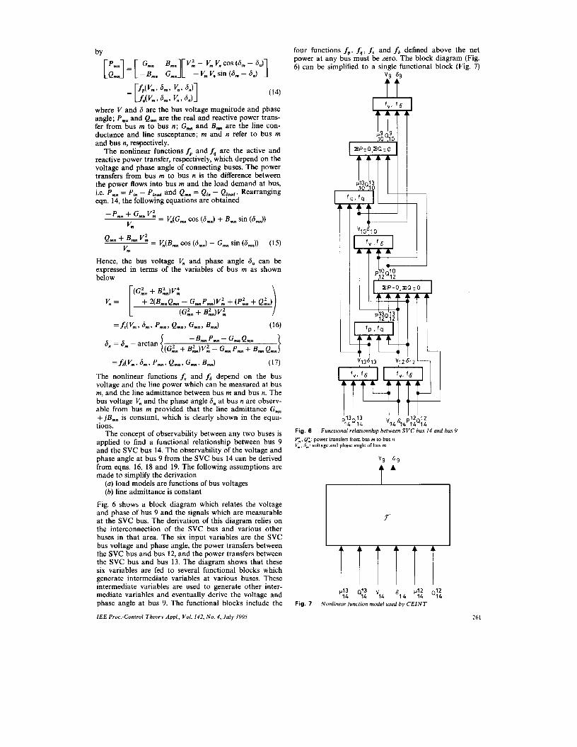
Fig. 6 shows a block diagram which relates the voltage and phase of bus 9 and the signals which are measurable at the SVC bus. The derivation of this diagram relies on the interconnection of the SVC bus and various other buses in that area. The six input variables are the SVC bus voltage and phase angle, the power transfers between the SVC bus and bus 12, and the power transfers between the SVC bus and bus 13. The diagram shows that these six variables are fed to several functional blocks which generate intermediate variables at various buses. These intermediate variables are used to generate other intermediate variables and eventually derive the voltage and phase angle at bus 9. The functional blocks include the

IEE Proc.-Control Theory Appl., Vol. 142, N o . 4 , July 1995

four functions f,, fq, f, and fa defined above the net power at any bus must be zero. The block diagram (Fig. 6) can be simplified to a single functional block (Fig. 7)

p13Q13 14 14 Vl4%1P:tQ:t

Fig. 6 Functional relationship between SVC bus 14 and bus 9 F.. Qm: power transfers from bus m to bus n V, , 6 , : voltage and phase angle of bus m

v3 63

t t

P,lz QiZ V,4 p:: Q!:

Fig. 7 Nonlinearfunction model used by C E I N T

261

where the CEINT network can model this unknown nonlinear function @: W6 + %*. The functional relationship 9 is static and thus the CEINT network uses an equation error model (Fig. la).

In general, the functional relationship obtained between the local variables and the remote variables will be a dynamic model if the system loads have dynamic models. The condition for observability is summarised in a lemma. The concept of a proper bus must be defined before the lemma is discussed.

Given a bus as the local bus, any other bus in the system can be classified as follows

(i) level 1 : buses connect directly to the local bus (ii) level 2: buses connect to the local bus via a level 1

(iii) level n: buses connect to the local bus via a level bus

n - 1 hiis

calculate all the bus voltages and line powers. For the four-machine power system (Fig. 4), if the SVC

bus is chosen as the local bus, the buses are classified as follows:

duration started at 0.1 s. The fault duration was chosen to cause large oscillation in the system response without allowing it to become unstable.

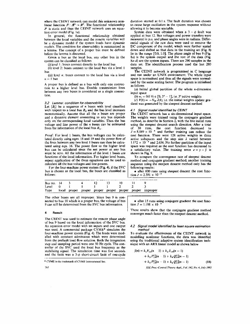
System data were obtained when a 3 - 4 fault was applied at bus 12. Bus voltages and power transfers were measured in p.u. and phase angles were in radians. Differ- ential signals of the raw data were used to remove the DC component of the model, which were further scaled down and shifted so that data in the training set (Fig. 8) lie in the range CO.0, 1.01. The phase angle of bus 9 (Fig. 8a) is the system output and the rest of the data (Fig. 8a-4 are the system inputs. There are 290 samples in the data set. The identification process used the last 280 samples.

The CEINT network is programmed in C language and run under an UNIX environment. The whole input mace is normalised and thus all the sienals were normal-

sequence using the steepest descent method only has the following results:

0 after 600 runs using steepest descent the cost function J = 2.391 x lo-'

.. . _ _ _ i k d by the same scaling factor. The p6gram is initialised as follows

(a) Initial global partition of the whole n-dimension input space

(b) wi = 0.0 Vi E r0. 3" - 11, i.e. 3" active weights

A proper bus is defined as a bus with only one connec- tion to a higher level bus. Double transmission lines between any two buses is considered as a single connec- tion.

The other buses are all improper. Since bus 9 is connected to bus 10 which is a proper bus, the voltage of bus 9 can still be determined from the SVC bus information.

, , . -. (c) V(1) = - V w j ( l ) , i.e. the initial weights update gra-

dient was generated by the steepest descent method 3.2 Lemma : condition for observability Let { B , } be a seguence of n buses with level classified

~

0 after 15 runs using conjugate gradient the cost function J = 1.198 x lo-'

4 Result

The CEINT was used to estimate the remote phase angle of bus 9 based on the local information of the SVC bus. An equation error model with six inputs and one output was used. A commercial package CYME* simulates the four-machine power system (Fig. 4). The loads were modelled with constant admittance which were determined from the prefault load flow solution. Both the integration step and sampling period were one 50 Hz cycle. The controller of the SVC used the local bus frequency as the stabilising signal. The simulation time was five seconds and the fault was a 3-4 short-circuit fault of one-cycle

1 These results show that the conjugate gradient method converges much faster than the steepest descent method.

4.2 Signal model identified by least square estimation method

To evaluate the effectiveness of the CEINT network in modelling nonlinear functions, the data was identified using the traditional adaptive system identification technique with an ARX linear model as shown below

j(n) = k , V,,(n - 1) + k , 6,,(n - 1)

+ k , P::(n - 1) + k,Q::(n - 1)

+ k , P::(n - 1) + k , Q::(n - 1) (18) CYME is the trademark of CYME International Inc.

262 IEE Proc.-Control Theory Appl., Vol. 142, No. 4, July I995

1 0 8

0 7 ” bus 14

samples 0

0 3 1

0 36

0 35

0 34

0 27 0 50 100 150 200 250 300

samples b

0 501 1

4 5 } P(bus 14-13) l

0 30

0 20 :::I , , , , , 1 0 05

0 50 100 150 200 250 300 samples

C

1 0 7 P(bus 14-12 i

samples d

Fig. 8 Training data set LI bus phase angle b bus voltage

IEE Proc.-Control Theory Appl., Vol. 142, No. 4, July 1995

c power flow from bus 14 io bus 13 d power flow from bus 14 io bus 12

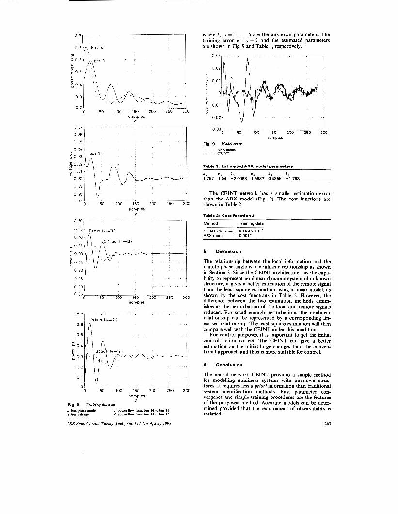
where k i , i = 1, . . . , 6 are the unknown parameters. The training error e = y - j and the estimated parameters are shown in Fig. 9 and Table 1, respectively.

0 03

I h h 3 a i 0.01

c 0 - 9

g -0.01 -

0

0 - 01

- 0 . 0 2 -

Table 1 : Estimated AAX model parameters

k , k , k , k4 k , k.3 1.757 1.04 -2.0083 1.5837 0.4255 -1.793

The CEINT network has a smaller estimation error than the ARX model (Fig. 9). The cost functions are shown in Table 2.

Table 2: Cost function J

Method Training data

CEINT (30 runs) 8.189 x ARX model 0.001 1

5 Discussion

The relationship between the local information and the remote phase angle is a nonlinear relationship as shown in Section 3. Since the CEINT architecture has the capability to represent nonlinear dynamic system of unknown structure, it gives a better estimation of the remote signal than the least square estimation using a linear model, as shown by the cost functions in Table 2. However, the difference between the two estimation methods dimin- ishes as the perturbation of the local and remote signals reduced. For small enough perturbations, the nonlinear relationship can be represented by a corresponding lin- earised relationship. The least square estimation will then compare well with the CEINT under this condition.

For control purposes, it is important to get the initial control action correct. The CEINT can give a better estimation on the initial large changes than the conventional approach and thus is more suitable for control.

6 Conclusion

The neural network CEINT provides a simple method for modelling nonlinear systems with unknown struc- tures. It requires less a priori information than traditional system identification methods. Fast parameter convergence and simple training procedures are the features of the proposed method. Accurate models can be determined provided that the requirement of observability is satisfied.

263

An application of CEINT to signal model identification of power system is presented and the identified model can be incorporated in the design of the power system controllers.

7 References

1 OLWEGARD, A., WALVE, K., WAGLUND, G., FRANK, H., and TORSENG, S.: ‘Improvement of transmission capacity by thyristor controlled reactive power’, I E E E Trans., 1981, PAS-100, (8). pp. 3930-3939

2 BYERLY, R.T., POZNANIAK, D.T., and TAYLOR, E.R.: ‘Static reactive compensation for power transmission systems’, I E E E Trans., 1982, PAS-101, (lo), pp. 3997-4005

3 HAMMAD, A.E.: ‘Analysis of power system stability enhancement by static VAR compensators’, IEEE Trans., 1986, PWRS-1, (4), pp. 222-227

4 OBRIEN, M., and LEDWICH, G.: ‘Static reactive-power compensator controls for improved system stability’, IEE Proceedings, 1987,134, (I), pp. 38-42

5 GYUGYI, L., OTTO, R.A., and PUTMAN, T.H.: ‘Principles and applications of static thyristor-controlled shunt compensators’, IEEE Trans., 1978, PA-97, (5), pp. 1935-1945

6 HAUTH, R.L., HUMANN, T., and NEWELL, RJ.: ‘Application of a static VAR system to regulate system voltage in Western Neb- raska’, I E E E Trans., 1978, PAS-97, (5). pp. 1955-1962

7 LOWE, S.K.: ‘Static VAR compensators and their applications in Australia’, Power Eng. J., 1989, pp. 247-256

8 GYUGYI, L., and TAYLOR, E.R.: ‘Characteristics of static, thyristor-controlled shunt compensators for power transmission system applications’, I E E E Trans., 1980, PAS-99, (5), pp. 1795-1804

9 PADIYAR, K.R., and VARMA, R.K.: ‘Damping torque analysis of static VAR system controllers’, IEEE Trans., 1991, P W m (3), pp. 45&465

10 LERCH, E., POVH, D., and XU, L.: ‘Advanced SVC control for damping power system oscillations’, I E E E Trans., 1991, P W W , (2). pp. 524-535

1 1 HUNG, L., and SODERSTROM, T.: Theory and practice of recursive identification’ (MIT Press, 1983)

12 NARENDRA, K.S., and PARTHASARATHY, K.: ‘Identification and control of dynamical systems using neural networks’, IEEE Trans., 1990, “-1, (I), pp. 4-27

13 QIN, S.Z., SU, H.T., and MCAVOY, T.J.: ‘Comparison of four neural net learning methods for dynamic system identification’, IEEE Trans., 1992, “-3, (l), pp. 122-130

14 MILLER, W.T., SUTTON, R.S., and WERBOS, P.J.: ‘Neural networks for control’(M1T Press, 1990)

15 SOBAJIC, D.J., and PAO, Y.H.: ‘Artificial neural-net based dynamic security assessment for electric power systems’, I E E E Trans., 1989, PWRS-4, (l), pp. 220-228

16 SANTOSO, N.I., and TAN, O.T.: ‘Neural-net based real-time control of capacitors installed on distribution of systems’, IEEE Trans., 1989, PD-5, (l), pp. 266-272

17 NIEBUR, D., and GERMOND, A.1.: ‘Power system static security assessment using the Kohonen neural network classifier’, IEEE Trans., 1992, PWRS-7, (2). pp. 865-872

18 MORI, H., TAMARU, Y., and TSUZUKI, S.: ‘An artificial neural- net based technique for power system dynamic stability with the Kohonen model’, IEEE Trans., 1992, PWRS-7, (2). pp. 856-864

19 KANDIL, N., SOOD, V.K., KHORASANI, K., and PATEL, R.V.: ‘Fault identification in an AC-DC transmission system using neural networks’, I E E E Trans., 1992, PWRS-7, (2), pp. 812-819

20 LIPPMANN, R.P.: ‘An introduction to computing with neural nets’, IEEE ASSP Mog., April 1987, pp. 4-22

21 ALBUS, J.S.: ‘A new approach to manipulator control: the Cerebel- lar articular controller (CMAC)’, Trans. A S M E J. Dyn. Syst., Meas. Control, 1975.97, pp. 220-227

22 BERGER, C.S.: ‘A general purpose modelling program’. Presented at IFAC, Sydney, 1993, preprinted edition. Vol. 10, pp. 381-384

23 WISMER, D.A., and CHATTERGY, R.: ‘Introduction to nonlinear optimization’ (North-Holland, 1978)

INSTITUTE OF MATHEMATICS AND ITS APPLICATIONS

PATRICK PARKS MEMORIAL MEETING A meeting will be held on Monday, 18th September 1995, to commemorate the work of Professor Patrick Parks, whose untimely death occurred in January this year. The meeting will be held in Somerville College, Oxford University, and will consist of an afternoon lecture series followed by dinner.

Invited speakers for the afternoon session include:

Professor H. Rosenbrock FRS (UMIST) Academician Y. Z. Tsypkin (Institute of Control, Moscow) Professor C. Harris (University of Southampton) Professor H. Tolle (University of Darmstadt, Germany) Professor J. Douce (University of Warwick) Professor K. Warwick (University of Reading) Professor B. White (Shrivenham)

The speakers have been selected so as to reflect the different fields of interest of Professor Parks, from Lyapunov stability theory to neural networks.

All are invited to attend both the afternoon lecture series and/or the evening dinner. Please contact Ms Pamela Irving at the Institute of Mathematics and its Applications, Catherine Richards House, 16 Nelson Street, Southend-on-Sea, Essex SS1 IEF, UK.

64 I E E Proc.-Control Theory Appl., Vol. 142, No. 4, July I995

Documents

Neural network approach to signal modelling in power systems