Networks formation to assist decision making · Networks formation to assist decision making David Goldbaum ... [email protected] 1. ... (2010) injects a time

Networks formation to assist decision making

David Goldbaum∗

April 29, 2016

Abstract

This paper examines network formation among a connected population with a preference for con-

formity and leadership. Agents build stable personal relationships to achieve coordinated actions. The

network serves as a repository of collective experiences so that cooperation can emerge from simple,

myopic, self-serving adaptation to recent events despite the competing impulses of conformity and lead-

ership and despite limiting individuals to only local information. Computational analysis reveals how

behavioral tendencies impact network formation and identifies locally stable disequilibrium structures.

Keywords: Leader, Dynamic Network, Payoff interdependence, Social Interaction, Simulation

(JEL Codes: D85, D71, C71)

∗Economics Discipline Group, University of Technology Sydney, PO Box 123 Broadway, NSW 2007 Australia,[email protected]

1

One does not become a guru by accident.

James Fenton1

1 Introduction

Sellers stylishly enhance functionally equivalent product offerings, thereby appealing to buyers’ subjective

tastes. The prevalence of experts offering guidance in subjective goods suggest social influences play a role in

decision making. In a number of settings, decision makers prefer conformity. What constitutes an expert of

a subjective good may simply be someone with an audience.2 Social influence invites strategies played over

social position, rather than over product choice, in order to achieve conformity, particularly if the preference

for conformity is enhanced by the appearance of influence over the decisions of others.3

With social interactions, when to act is as much an element of strategy as how to act. Social positioning

cannot arise spontaneously. Repeated decisions, like those offered with each new fashion season, offer op-

portunity for social repositioning and reputation. This paper investigates the evolution in social positioning

over time via a network of links as players seek to achieve conformity and leadership.

A utility-based desire for conformity can be modeled as arising out of a social component, such as in

Brock and Durlauf (2001). With modification, the social component also provides a utility reward to early

adopters based on the population of matching subsequent adopters, as in Goldbaum (2016).

The inability to employ a consistent language with which to refer to the ever-changing targets of coordi-

nation makes the product-space strategies employed in the coordination game of Crawford and Haller (1990)

unavailable to the agents in the current model. A network of reliable social connections is the foundation

upon which the agents develop strategies to facilitate coordination.

The social network has long been recognized as a vehicle for coordinating activities. Social networks

generate by-directional interactions between local and aggregate behavior. For Schelling (1971), Schelling

(1973), and Katz and Shapiro (1985) the individual discrete decisions are sensitive to the information available

through network connections, influencing which new products or technologies are adopted. Because of social

interactions, products that garner no particular consumer preference can grow to dominate consumer choice.

1Columbia World of Quotations. Columbia University Press, 1996. http://quotes.dictionary.com/Onedoesnotbecomeagurubyaccident(accessed: March 17, 2011).

2A guru is “a teacher who attracts disciples or followers.” An expert is “a person who has special skill or knowledge in someparticular field; specialist; authority.” (Dictionary.com, 2016) Maybe more guru than expert.

3“Wine geeks just love bragging rights. They get kudos from their peers when they get a high-score wine first or getit cheaper” (Bialek quoted in Los Angeles Magazine, 1998(Dec)). The social component of acting in advance of a trend ishighlighted as distinct from a simple desire to adopt products when they are new, a desire that is not necessarily sociallyderived.

2

A network is also a vehicle for information transmission as, for example, the Ellison and Fudenberg (1995)

use of an undirected network and in the directed network of Dutta and Jackson (2000).

Consensus and information transmission are at the heart of the DeGroot (1974) social learning model.

The social network is a conduit of information by which populations update beliefs in an effort to eliminate

private biases. The ability of privately informed linked individuals to reach consensus on the truth depends

on the structure of the network. As identified by Corazzini et al. (2012), individuals with outsized influence

facilitate convergence while impeding the emergence of the truth unless they are also well-connected gatherers

of information.

The Acemoglu et al. (2013) extension to the social learning model finds that a population subset which

retains its private opinion impacts beliefs and convergence, as one might expect from an opinion leader.

Acemoglu et al. (2010) injects a time element with agents pressed to act on their beliefs by a penalty for

delaying adoption. Arifovic et al. (2015) identifies a preference for consensus affecting the updating of beliefs.

Inherent in the social learning models is an intrinsic truth that each agent wishes to learn. As a Bayesian

or employing some non-Bayesian alternative, they look to make use of every bit of information available to

them to uncover the truth. In the current setting, there is no truth, only a social construct. The social

learning mechanism of gathering and aggregating information does not serve the individual’s objectives for

conformity and influence.

Ali and Kartik (2012) introduces a preference over the actions of others to the model of observational

learning. Borrowing one of the authors’ examples, the model applies to agents making political contributions

to gain favor from the winning candidate. With learning, early contributors influence the target of subsequent

contributions, affecting election outcomes. Later contributors have an informational advantage about which

candidate is likely to win based on prior support. Following the original model of Banerjee (1992), Ali and

Kartik (2012) have agents decide sequentially. Pushing the scenario beyond the original example, it would

be reasonable to allow the politician to place grater value on early contributions, knowing the potential

influential impact it can have on downstream contributors. This creates a tradeoff between contributing

early or delaying. Freeing contributors to choose the timing of a contribution increases the uncertainty,

particularly when contributions can be made simultaneously, as contributors cannot know the value of their

contribution on subsequent decision makers.

Achieving conformity requires forming a purposeful network for transmitting and receiving information.

In the developed model, agents establish one-sided directed links in order to receive information on the

adoption decision of the link’s target as a means to generate coordination. New linking decisions are made

3

simultaneously for the current adoption decision. Each agent evaluates her decision ex post based on the

outcome versus counterfactual payoffs offered by other linking options and of choosing autonomously. This

ex post evaluation informs the agent’s linking decision for the next adoption decision. This paper investigates

environmental influences on the ability of the population to develop a coordinating network. Also explored

are individual characteristics as they affect individual positioning in the emergent network.

The simultaneous, rather than sequential, linking decisions avoids exogenously imposed advantages in

positioning. This precludes the network formation process based on ordered sequential linking decisions

of Jackson and Wolinsky (1996), Watts (2001) and related works. Bala and Goyal (2000) allows myopic

best-response one-sided link formation by randomly chosen agents with full knowledge of the network. The

current investigation envisions the game played by a potentially large population, where knowledge of the

full network is unknowable or impractical. Agents have access to aggregate information concerning previous

realizations of popularity but only local knowledge about individual adoptions and payoffs. Nonetheless, the

leader-centric star network (or, more properly given limited linking options, a leader-centered hub) is the

natural target structure for its ability to coordinate activity.

Like Chang and Harrington (2007), a symbiotic relationship emerges according to roles individuals find

themselves in. Agents adapt to their changing local environment in a payoff improving manner. Simulations

characterize the behavior of the population. Individual strategies are modeled as evolving according to the

Experience Weighted Attractor (EWA) of Camerer and Ho (1999). Agents employ actions probabilistically

according to a nested logit model of Hausman and McFadden (1984). Both models have strong foundations

in evolutionary and discrete choice modeling. This paper develops the dynamic environment and explores

computationally the variety of processes and outcomes as determined by different combinations of the EWA

and nested logit model parameters. An individual’s characteristics can inform local experiences but aggregate

outcomes are the product of the environment.

2 Model

Let N = {1, . . . , n} be a set of agents. Let O(t) = {O1t, O2t, . . . , Omt} be a new set of options available

in time period t. In each time period, t ∈ {1, . . . , T}, each agent looks to adopt from one of the options.

Let K = {“A”, “B”,. . . } be a set of m labels for these options and let the private one-to-one function fi,t,

determined by nature, map from labels to options, fi,t : K → O(t). Each player thus privately observes

the K set of labeled options. Each player sees different labels and for every i, j pair there is a one-to-one

4

function hi,j,t : Ki,t → Kj,t that is unknown to the players. The mechanism prevents coordination between

agents on a particular choice, either through prior communication, or by identifying a focal point.

Visibility across the population is limited to individual contact lists which identify, for each agent, who

in the population they can directly observe. Thus, agent i can observe agent j’s adoption of O(t) only if

agent j is on i’s contact list. Let Nd(i) ⊆ N represent i’s contact list. Let the adjacency matrix g capture

the network of contact links where element gij = 1 if j ∈ Nd(i) and zero otherwise. Let nd indicate the

number of contacts for each agent, nd = |Nd(i)|.

Let ai,t denote the action of player i in period t. Players act simultaneously with each player choosing (i)

one of the m options, or (ii) to link to another player. In the former case, if player i chooses option Ok,t, then

assign ai,t = f−1i,t (Ok,t). If player i links to player j, then assign ai,t = j. A player who chooses an option is

said to lead while a player who links to another is said to imitate or follow the other player. An agent who

leads and has followers is referred to as a leader. Thus, the set of actions for player i is Ai = Ki ∪ Nd(i).

Write a = (a1, . . . , an), for an action profile, where ai ∈ Ai.

Each ai ∈ Nd(i) represents a decision to imitate the targeted individual. Let σ represent the adjacency

matrix produced by imitative actions so that σij = 1 if ai = j and zero otherwise. Refer to σ as the social

structure for capturing who leads and who follows whom. Let Σ represent the set of σ in which there is a

single leader and the remaining n−1 agents follow the single leader, directly or indirectly through a series of

links. Let Σ∗ ⊆ Σ be the set of structures in which each follower is at the minimum distance possible from

the leader measured in links according to the available contacts.

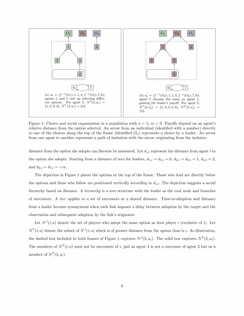
Example 1. The two frames of Figure 1 present two possible realizations generated from the same set

of underlying actions. The population consists of n = 7 agents facing m = 3 options. The action set is

a = (”A”, 1, 1, 3, ”C”, 7, 6). That is, both agents 1 and 5 lead, agents 2 and 3 imitate agent 1, agent 4

imitates agent 3, agents 6 and 7 imitate each other. These actions determine the social structure for the

period. Only agent 1 is a leader, having a non-trivial population of followers. Agents 2, 3, and 4 are followers

of 1. Agent 5 leads, but is not a leader. Agents 6 and 7 are within a self-referencing loop.

What distinguishes the two realizations is the mapping from labels to options. In 1a, agents 1 and 5

select different options according to nature’s determination of O1 = f1(A) and O3 = f5(C). In 1b, agents 1

and 5 select the same option according to nature’s determination of O2 = f1(A) = f5(C).

Allow that i is a predecessor of j and j is a successor of i in the structure σ if j imitates i, either directly

or indirectly through a chain of imitators. Let di,j,t represent the distance from agent i to agent j measured

in the number of links that separate them. From Example 1, d2,1,t = d3,1,t = 1 and d4,1,t = 2. An agent’s

5

O1 O2 O3

1 5

2 3

4

6 7

(a) at = (f−1(O1), 1, 1, 3, f−1(O3), 7, 6);agents 1 and 5 end up selecting differ-ent options. For agent 2, NJ (2, at) ={1, 2, 3, 4}, NT (2, at) = {4}.

O1 O2 O3

1 5

2 3

4

6 7

(b) a′t = (f−1(O2), 1, 1, 3, f−1(O2), 7, 6);

agent 5 chooses the same as agent 1,gaining the leader’s payoff. For agent 2,

NJ (2, a′t) = {1, 2, 3, 4, 5}, NT (2, a

′t) =

{4}.

Figure 1: Choice and social organization in a population with n = 5, m = 3. Payoffs depend on an agent’srelative distance from the option selected. An arrow from an individual (identified with a number) directlyto one of the choices along the top of the frame (identified On) represents a choice by a leader. An arrowfrom one agent to another represents a path of imitation with the arrow originating from the imitator.

distance from the option she adopts can likewise be measured. Let di,t represent the distance from agent i to

the option she adopts. Starting from a distance of zero for leaders, d1,t = d5,t = 0, d2,t = d3,t = 1, d4,t = 2,

and d6,t = d7,t = +∞.

The depiction in Figure 1 places the options at the top of the frame. Those who lead are directly below

the options and those who follow are positioned vertically according to di,t. The depiction suggests a social

hierarchy based on distance. A hierarchy is a tree structure with the leader as the root node and branches

of successors. A tier applies to a set of successors at a shared distance. Time-to-adoption and distance

from a leader become synonymous when each link imposes a delay between adoption by the target and the

observation and subsequent adoption by the link’s originator.

Let NJ(i; a) denote the set of players who adopt the same option as does player i (exclusive of i). Let

NT (i; a) denote the subset of NJ(i; a) which is of greater distance from the option than is i. As illustration,

the dashed box included in both frames of Figure 1 captures NJ(2, at). The solid box captures NT (2, at).

The members of NT (i; a) need not be successors of i, just as agent 4 is not a successor of agent 2 but us a

member of NT (2, at).

6

Let nJi,t and nTi,t represent the size of the respective NJ(i; a) and NT (i; a) sets. The payoff for player i is

πi(σ) = aJnJi,t + aTn

Ti,t (1)

with coefficients aT ≥ 0 and aJ ≥ 0. The first element of the payoff is the “conformity” component, much like

the community effect of Blume and Durlauf (2001). The second element in (1) reflects the distance/timing

advantage a player has over other players. By (1), an individual’s payoff is purely a social phenomenon. The

options themselves offer no direct benefit to the agent.

Autarky, the consequence of everyone leading, generates expected payoffs of aJ(n − 1)/m. The full

coordination produced by the entire population formed into a single hierarchy generates individual payoffs

ranging from (aT + aJ)(n− 1) for the leader to aJ(n− 1) going to the most distant follower(s). The benefit

over autarky to even the lowest compensated agent illustrates the benefit to coordinating.

Let

B := θ −(

1− 1

n− 1

)with θ = (m−1)aJ/aT . The parameter θ reflect the relatives strength between the attraction for conformity

and the attraction to lead. The most distant successors are attracted to lead when the premium to acting in

advance of followers is high (so that aJ/aT is low) or when m is small, yielding a high probability of choosing

the same as the leader.

The set of equilibrium structures always includes a single hierarchy structure. The equilibrium size of

the hierarchy increases with B with B ≥ 0 inducing the entire population to join in following the single

leader. Abandonment of the hierarchy by followers is from the bottom as an already negative B decreases.

The equilibrium hierarchy size for B < 0 has a number of followers, n∗s < n−1 with n∗s an integer value near

1/(1− θ).

If the equilibrium structure is going to emerge in the simultaneous decision setting, then it has to emerge

from path dependent play. Simulations are employed to investigate dynamic behavior and adjustment to

explore possible paths of individual behavior and group organization.

For the dynamic simulation, each agent chooses from the available actions probabilistically. In period t,

for ρi,t ∈ [0, 1] ,

ρi,t = Pr(i leads)

(1− ρi,t)wji,t = Pr(i follows j) j ∈ Nd(i),

7

where∑j∈Nd(i) w

ji,t = 1, wji,t ∈ [0, 1]∀i, j. For those agents who lead, a simple random assignment for

determining ki,t ∈ Ot captures the inability to coordinate on an initial choice.

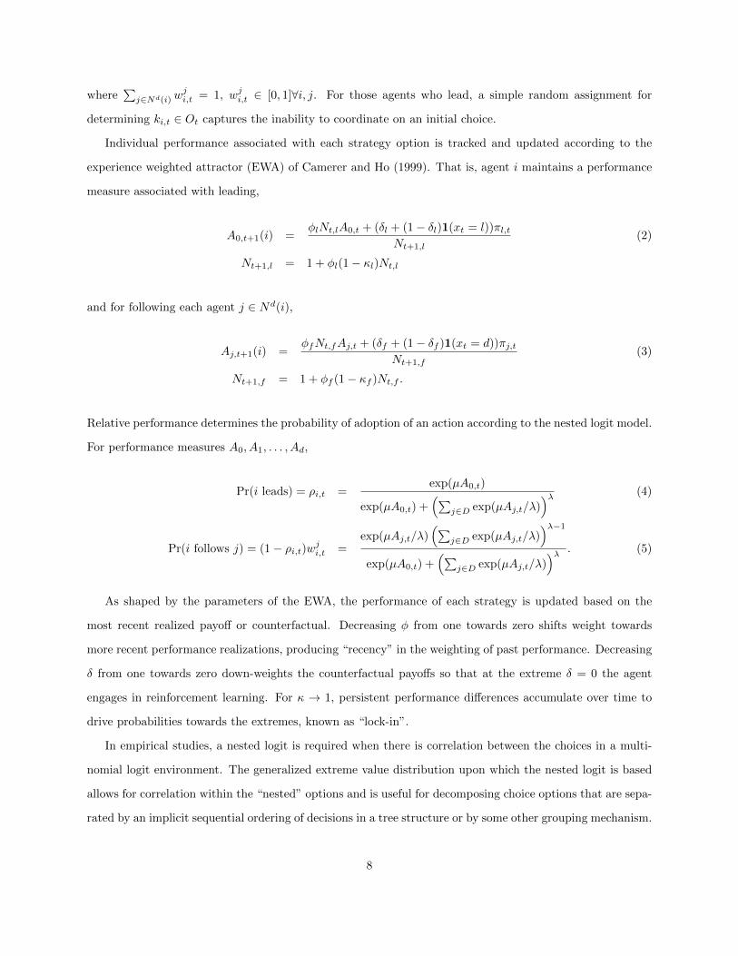
Individual performance associated with each strategy option is tracked and updated according to the

experience weighted attractor (EWA) of Camerer and Ho (1999). That is, agent i maintains a performance

measure associated with leading,

A0,t+1(i) =φlNt,lA0,t + (δl + (1− δl)1(xt = l))πl,t

Nt+1,l(2)

Nt+1,l = 1 + φl(1− κl)Nt,l

and for following each agent j ∈ Nd(i),

Aj,t+1(i) =φfNt,fAj,t + (δf + (1− δf )1(xt = d))πj,t

Nt+1,f(3)

Nt+1,f = 1 + φf (1− κf )Nt,f .

Relative performance determines the probability of adoption of an action according to the nested logit model.

For performance measures A0, A1, . . . , Ad,

Pr(i leads) = ρi,t =exp(µA0,t)

exp(µA0,t) +(∑

j∈D exp(µAj,t/λ))λ (4)

Pr(i follows j) = (1− ρi,t)wji,t =exp(µAj,t/λ)

(∑j∈D exp(µAj,t/λ)

)λ−1exp(µA0,t) +

(∑j∈D exp(µAj,t/λ)

)λ . (5)

As shaped by the parameters of the EWA, the performance of each strategy is updated based on the

most recent realized payoff or counterfactual. Decreasing φ from one towards zero shifts weight towards

more recent performance realizations, producing “recency” in the weighting of past performance. Decreasing

δ from one towards zero down-weights the counterfactual payoffs so that at the extreme δ = 0 the agent

engages in reinforcement learning. For κ → 1, persistent performance differences accumulate over time to

drive probabilities towards the extremes, known as “lock-in”.

In empirical studies, a nested logit is required when there is correlation between the choices in a multi-

nomial logit environment. The generalized extreme value distribution upon which the nested logit is based

allows for correlation within the “nested” options and is useful for decomposing choice options that are sepa-

rated by an implicit sequential ordering of decisions in a tree structure or by some other grouping mechanism.

8

In a simulation setting the nesting serves as a mechanism for compartmentalizing components of a decision.

The parameter µ is commonly referred to as the intensity of choice (IOC) parameter. It determines

how sensitive an agent is to differences in the performance measure. At µ = 0, the agent is indifferent to

the choices regardless of the performance. As µ increases, for a fixed performance differential, the agent’s

probability of adopting the superior strategy increases.

The λ parameter controls the extent to which the agent compartmentalizes the decision about whether

to lead or follow from the decision about who to imitate when following. Nesting addresses the independence

of irrelevant alternatives problem in multinomial logit problems. The nested logit allows for the introduction

of a new contact to draw probability weight from the other contacts in different proportion than it draws

from the option to lead.

The advantage of the EWA and nested logit combination is that the models are well grounded empirically

and have been used extensively for estimating human behavior in a wide range of discrete choice settings.

The model performs poorly when examined using a discrete choice model without nesting because it forces

a single IOC parameter to capture the intensity of both the decision about whether to lead or follow and the

decision about who to follow. Completely separating the decision about whether to follow from the decision

about who to follow using a two step decision process lacks this empirical foundation and, in particular, fails

to preserve independence from irrelevant alternatives.4

Once actions have been determined for the period, the action-dependent social network structure σ can

be constructed, option selection by leaders made, and payoffs computed according to (1). The EWA updates

the performance measures of the untried options as well as the options employed. For the former, the agents

need to estimate the payoff that would have been earned with each of the counterfactual actions. Ex-post, the

agents can observe which option each member of their contact list adopted and when, within the period, this

adoption took place. With knowledge about aggregate popularity of each option as it disseminates through

the population, the agents can place themselves in the position of having imitated each contact and guess

at the position dependent counterfactual payoff earned, treating the time of adoption for all others as given.

4A variety of alternatives to the combined EWA and nested logit are available for dynamically modeling strategy adjustment.Also modeled, but not included for presentation in this paper, were two versions of a two-stage decision process with separateEWA processes for determining the value of ρi,t and for determining the value of wj

i,t. The two-stage decision was investigated

using both the Camerer and Ho (1999) specified power distribution for allocating probabilities based on the performancemeasures as well as an alternate method based on a k-choice replicator dynamics derived from Branch and McGough (2008).The latter is considerably more resilient at achieving the equilibrium structure from a variety of starting conditions andenvironment setting than is the EWA and nested logit combination.

9

3 Simulations

3.1 Measuring organizational success

One measure of how close the population has come to adopting equilibrium strategies is to look at the

number of agents who lead. Let µlead,t be the number of agents who lead in period t. For B ≥ 0, µlead,t = 1

in equilibrium. Another measure of success is to consider each agent’s distance from their chosen leader. A

minimal distance social structure is one in which each follower chooses to rely on the contact offering the

shortest distance to her leader.

Recall that dj,i,t represents agent j’s distance measured in number of links from leader i in period t,

let dj,i,t indicate the shortest possible distance available to player j given the linking decisions of the other

agents. Let ∆t, referred to as the ∆-inefficiency score, measure aggregate deviations from minimal distance

according to

∆t =∑j

dj,i,t − dj,i,t. (6)

Accordingly, ∆t = 0 represents a social structure in which each follower employs the shortest distance to her

leader. Values of ∆t > 0 indicate deviations from minimal distance. A third related measure of the proximity

to the equilibrium structure is how many in the population are caught in a self-referencing imitation loop.

Let µloop,t represent the number of agents caught in a self-referencing loop.

The variation in the parameters across different treatments leaves B unchanged, and thus only affects

the evolutionary process of the population and not the equilibrium target.

3.2 Behavior effects

This section presents simulations of a relatively large homogenous population distributed over a randomly

generated, strongly connected, directed network capturing individual contact lists. Table 1 reports the model

treatments considered.

Frequencies with which each treatment achieves or nearly achieves the equilibrium structure are de-

rived from Monte Carlo simulations. An illustrative example of each treatment is presented and discussed

qualitatively.

For B � 0, there is a strong incentive to seek conformity and comparatively weak incentive to lead. In

such a reward setting, simulations quickly achieve the cooperative structure for an expansive combination

of the adaptive parameters. More interesting is a B that is just above or any B < 0. At certain positions in

10

Table 1: Simulation Treatments

Treatment Base 1 2 3 4 5 6 7 8 9 10 11

Population n 100

Number of contacts nd 6

Number of options m 12

Periods T 500 500 500 500 1000 500 500 500 500 500 500 500

Conformity reward aJ 0.2 0.1 0.1 0.1 0.1 0.1 0.1 0.1 0.1 0.1 0.1 0.1

Preemption reward aT 1

Participation B 1.21 0.11 0.11 0.11 0.11 0.11 0.11 0.11 0.11 0.11 -0.06 -0.06

Eq. Hierarchy size n∗s 100 100 100 100 100 100 100 100 100 100 15 15

Recency (L) φl 0.9 0.9 0.9 0.9 0.99 0 0.9 0.9 0.9 0.9 0.9 0.99

Recency (F) φf 0.9 0.9 0.9 0.9 0.99 0 0.9 0.9 0.9 0.9 0.9 0.99

Lock-in (L) κl 0 0 0 0 0.2 0 0 0 0 0 0 0.2

Lock-in (F) κf 0 0 0 0 0.2 0 0 0 0 0 0 0.2

Reinforcement (L) δl 1 1 1 1 1 1 0.2 1 1 1 1 1

Reinforcement (F) δf 1 1 1 1 1 1 1 0.7 1 1 1 1

Prior on leading A0(0) 0 0 0 0 0 0 0 0 0 3.5 0 0

Intensity of choice µ 1 1 3 0.05 0.2 0.6 1 1 1 1 0.6 0.2

Independence λ 0.9 0.9 0.9 0.9 0.9 0.9 0.9 0.9 0.15 0.9 0.9 0.9

iterations 200 200 200 200 200 200 200 200 200 200 200 200

Freq. ns = 99 0.995 0.470 0.705 0 0.980 0.305 0.995 0 0 0.400 0.025 0

Freq. ns ≥ 95 1 0.810 0.770 0 0.995 0.575 1 0 0 0.840 0.335 0.005

Freq. ns ≥ 50 1 0.990 0.805 0.120 0.995 0.965 1 0.485 0.48 0.985 1 0.470

the social structure, the differential by which between following and leading is small. How individuals and

those around them process information can impact imitation network evolution and outcomes.

A wide range of behaviors produce regular emergence of a near-equilibrium social structures. Consistently

producing the exact equilibrium structure requires a narrower set of parameters, particularly as B → 0 from

above and for B < 0.

The ex ante homogeneity causes players to employ identical first-period probabilities in identifying an

action. The different personal experiences in the first and subsequent periods lead to individual updating

of probabilities and thus ex post heterogeneity. Through this process, transitive events have potentially

permanent consequences by becoming embedded in the social network. For a leader to emerge, others in the

population must adjust ρi and wji,t ∀j ∈ Nd(i) to chase success. The process of observation and adjustment

allows the initially lucky individual to become a successful leader. The established leader is ensured of a

good outcome in each decision round, no longer reliant on luck but empowered by her followers. The success

in generating the equilibrium structure is in its backwards-looking measure of performance and the induced

adjustments in strategy that reward success with more success.

Figure 2 displays the typical first period structure under three different scenarios capturing the impact

11

(a) No nesting, no bias: λ = 1, A0,0 = 0 (b) Nesting: λ = 0.1, A0,0 = 0 (c) Bias: λ = 1, A0,0 = 5

Figure 2: Initial structure at t = 1: (2a) With independence across decisions and no bias, ρi = 0.14∀i.Long chains of followers with multiple branches produce considerable heterogeneity in t = 1 individual’sexperiences that feed into t = 2 decisions. (2b) With near-complete nesting, ρi = 0.46∀i. Long chains arepresent but multiple agents choose the same options, obscuring to the decision makers which agent has thefollowers. (2c) With a preference to lead producing ρi = 0.96∀i, there is minimal differentiation in payoffs.

of nesting and of a predisposition to leading

3.2.1 Baseline

The important feature of the baseline treatment is the relatively strong preference for conformity. The B =

1.2 is sufficiently large so that following stands out as an attractive option supported by prior experiences.

Once the hierarchy is formed with σ ∈ Σ, the most distant follower observes from personal experience that

the certain conformity that comes from following offers greater reward than the expected value of leading.

With the strong incentive for conformity, the process of emergence to the coordinating structure is robust

to a wide range of possible behavioral model parameters. For illustrative purposes, the EWA parameters

employed in this treatment are chosen to unbiasedly reflect underlying differences in performance. The

agents employ long memory and give full weight to counterfactual payoffs of the untried actions, but these

features are not essential.

The frames of Figure 3 present information capturing the evolution and eventual outcome from a chosen

revealing simulation. The sparse 3a reveals the speed with which the population joins in following a single

leader so that the three measures of µlead, µloop, and ∆ all quickly drop to zero. Frame 3b shows the social

structure as realized in the terminal period. Frames 3c-3f present the time-series of the performance measures

for the leader and select individuals based on their final distance from the leader. The overwhelming desire

for conformity ensures that for even the most distant follower, following clearly dominates leading. The

highly differentiated payoffs in the first period, as seen in Figure 2a, facilitate quick identification of a single

leader and evolution to the equilibrium structure.

12

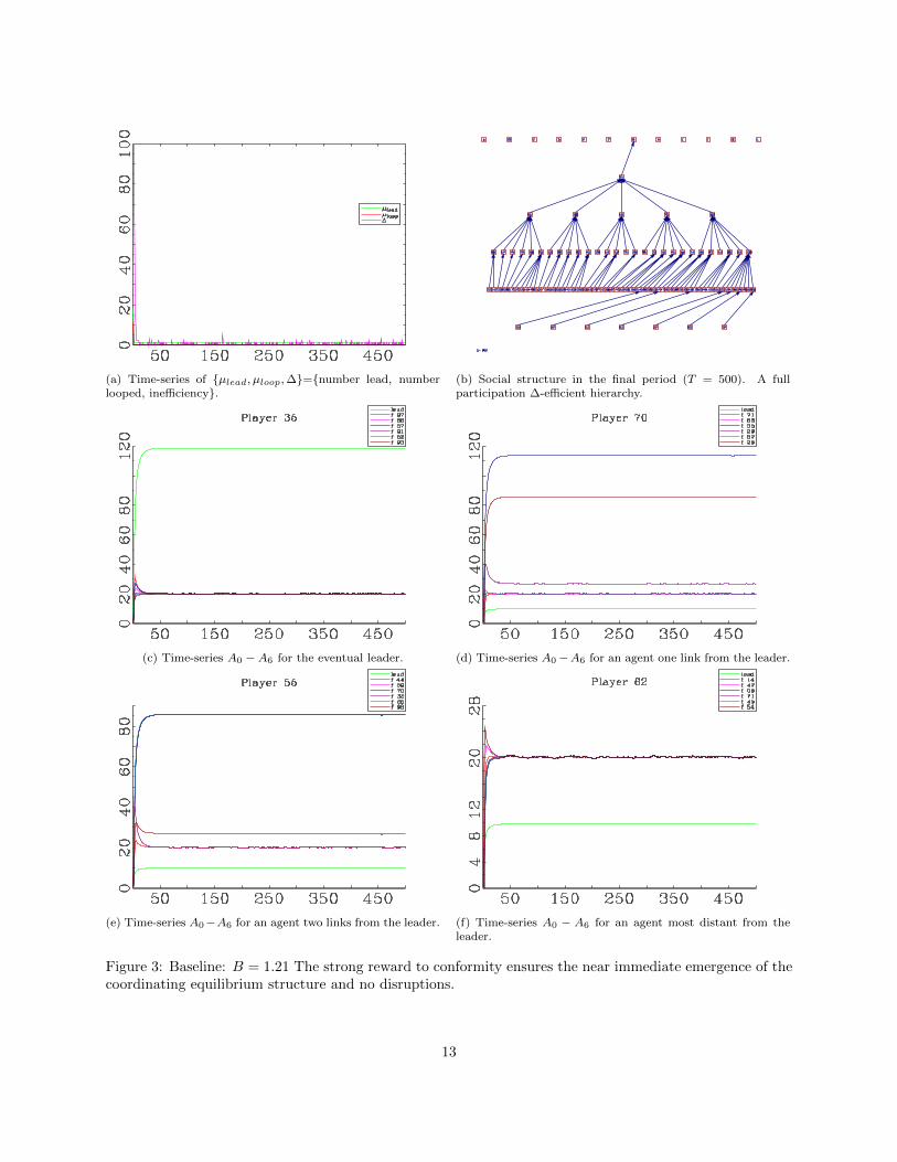
(a) Time-series of {µlead, µloop,∆}={number lead, numberlooped, inefficiency}.

(b) Social structure in the final period (T = 500). A fullparticipation ∆-efficient hierarchy.

(c) Time-series A0 −A6 for the eventual leader. (d) Time-series A0−A6 for an agent one link from the leader.

(e) Time-series A0−A6 for an agent two links from the leader. (f) Time-series A0 − A6 for an agent most distant from theleader.

Figure 3: Baseline: B = 1.21 The strong reward to conformity ensures the near immediate emergence of thecoordinating equilibrium structure and no disruptions.

13

The one instance out of 200 iterations, in which ns 6= n − 1 consists of two followers were caught in

a self-referencing loop, following each other in an attempt to link indirectly to the leader. There were no

instances where an agent other than the leader led in the final period.

3.2.2 Conformity vs influence

In Treatment 1, lowering aJ decreases B to 0.11. As long as B > 0, the target Nash equilibrium structure

is unchanged but for B close to zero, the payoff differential narrows, hindering identification of the superior

action. Narrow performance differentials generate indecisiveness in a logit model with the inferior action

garnering non-zero probability. This can potentially hinder evolution towards the equilibrium structure. Even

if a leader is identified, the most distant followers, for whom following only narrowly dominates leading, are

likely to remain irregular followers.

The most distant follower experiences one of three events each period. These are evident in the time-series

of performance measures presented in Figure 4f. Following is the most common action, earning a payoff of

aJns. To lead and match the leader, earning a payoff of aJns + aT (ns − 1), produces a spike up in A0. To

lead and fail to match the leader, earning a payoff of zero, produces a dip in A0.

Presented in Figure 4 is one of only two instances in which the structure deviated considerably from the

equilibrium. Here, the simulation is allowed to run for 800 periods to let the major disruption occurring

around t = 475 to play out. Though the disruption lasts for 200 periods, the population does return to

the near-equilibrium structure. In the other instance (not graphed), the emergent dominant leader has only

three direct followers, less than the average of six. From the onset, the followers remain in a seemingly stable

structure in which there remains a persistent population of 20-40 who lead rather than follow. At about

t = 700, the population quickly transitions to form into a near-equilibrium structure.

3.2.3 Intensity of choice

Treatment 2 is based on an increase to the IOC parameter, µ. The treatment is a possible counter to

the diminished performance differential between leading and following observed in Treatment 1. Increasing

µ, though, does not return the system to rapid convergence on the equilibrium structure. Compared to

Treatment 1, increasing the IOC parameter increases the likelihood of achieving the equilibrium structure.

It also increases the frequency with which little or no social structure emerges. Among the 20% of the runs

that fail to produce at least 50 followers in the dominant hierarchy, 5% terminate having settled into a

revolving population of only 10-20 agents following each period. The other 15% of the runs settle into an

14


(b) Social structure in the final period (T = 800).



Figure 4: Small preference for conformity: With B = 0.11 > 0 the reward to conformity remains strongerthan the desire to lead but the small differential produces indecision among the most distant followers aboutwhether to lead or follow, resulting in random adoption.

15

apparently stable structure consisting of a single dominant leader but with only a fraction of the population

following. Further increases in µ further increase the frequency in which no leader attracts a majority of the

population as followers.

Extending the duration of the simulation provides the opportunity to achieve the more cooperative

structure. Half of the runs with fewer than 50 followers at t = 500 achieve the equilibrium structure when

allowed to run 5,000 periods. One such run, presented in Figure 5 has no structure at time t = 500. Around

t = 1000 the population shifts to a state in which a single leader leads a small but stable population of tier

1 followers. Around t = 4670, there is another transition adding a second tier of followers to the hierarchy,

quickly followed by a third. The transitions are quick, taking five periods or so each. The overall impression

is that of a system transitioning through a series of locally stable disequilibrium structures before finally

achieving an equilibrium cooperative structure. The possibility of a stable disequilibrium is developed in

subsection 3.2.8.

Allowed to run for 10,000 periods, there remaining 11 runs that still fail to converged to the cooperative

structure. All look to be in the locally stable disequilibrium consisting of a leader and single tier of followers.

Decreasing the IOC parameter for Treatment 3 decreases agent sensitivity to performance differentials.

At a sufficiently low value, individual adjustment fails to respond to transitory random events sufficiently to

create permanent social advantage. The result is a population that remains perpetually disorganized. The

social structure in the last period is the same characteristically random structure as observed in the first, as

seen in 2a.

3.2.4 Lock-in

Treatment 4 introduces lock-in. The lock-in parameter adjusts how the agents aggregate performance in-

formation over time. Let πδh,t reflect the performance of strategy h = f, l in period t after discounting

counterfactual estimates according to δh. Thus,

πδh,t = (δh + (1− δh)1(xt = h))πh,t.

The impact of lock-in on the performance measure can be seen by examining the formula for the realized

Ah,t+1, where, for h ∈ {0, 1, . . . , d},

Ah,t =

(t−1∑s=0

(φh(1− κh))s

)−1(t−1∑s=0

(φsπδh,t−s)

). (7)

16


(b) Social structure in the final period (T = 5000). Eachdistance dj,i = 3 followers has a small probability of endingup at distance 4 but never lead.



Figure 5: Increase IOC: ↑ µ introduces instances in which the population appears to settle at a stabledisequilibrium structure.

17

For κh = 0, Aht reflects the average of weighted past performances. For κh = 1, Ah,t reflects an accumulation

of past performances. The distinction is that for κh = 0, the expected performance differential is the average

of the past performance differences, with the weighted sum of the past performances divided by the sum of the

weights. For κh = 1, the expected performance differential is the sum of the past differences. Accumulating

past performance rather than averaging allows a persistent differential to accumulate greater performance on

the superior option. The process could be interpreted as an increase in confidence through the accumulation

of information that allows the agent to put greater probability on the superior performing action.

For a πh,t drawn from a stationary distribution with mean πh, then for φ < 1, Ah,t converges to a

stationary distribution around a fixed mean value,

Ah =1− φh(1− κh)

1− φhπh. (8)

For a κ 6= 0 to meaningfully impact behavior requires the long memory produced by φh at or near one.

The infinite memory implied by φ = 1 and κ = 1 ensures that a consistently perceived dominating action

eventually attracts all of the probability weight, even for finite µ. From (8), κh > κ−h generates an asymptotic

bias in favor of the h associated action.

Finite machine measurability precludes simulating φ = 1 and κ = 1. Thus, the treatment employs

φ = 0.992 and κ = 0.2. Two additional accommodations lower µ and increase the length of each run

to T = 1000. The longer run provides time for an accumulation of evidence while the lower µ keeps the

nested logit computed probabilities machine measurable. This combination of features substantially raises

the incidence of emergence of the equilibrium structure. Instances in which the system settles at one of the

locally stable disequilibria still arise. The accumulation effect of employing lock-in can be seen in the rising

trend of the performance measure in Figure 6.

3.2.5 Recency

Treatment 5 introduces recency by setting φl = φf = 0. A leader emerges as behavior reinforces positive

experiences. Individual memory is not essential in this process as the network grows to reflect individual

experiences. Increasing recency by lowering φ leaves in place the ability to generate a dominant leader but

introduces instability in the social structure. The non-zero probability to lead means that there is always

deviation from the equilibrium structure. The absence of memory opens the possibility that the randomness

in the realized structure sufficiently changes incentives to permanently disrupt an existing social structure,

18





Figure 6: Lock-in: κl = κf = 0.2. The compounding of evidence allows the most distant followers torecognize the superiority of following.

19

allowing a new leader to emerge.

The leader at the end of the example presented in Figure 7 only came to be leader around t = 380. Prior

to this, there had been other leaders, including the agent depicted in Figure 7f.

3.2.6 Reinforcement

A tendency towards the use of reinforcement learning potentially undermines social adaption necessary to

generate the equilibrium structure. The evolution works when the population adjusts towards historically

high paying alternatives. With reinforcement learning the agents remain loyal to any action with a positive

payoff, generally missing opportunities for improvement, particularly as they might arise in a changing social

structure.

Treatment 6 introduces reinforcement learning in the decision to lead. Discounting the counterfactual

performance associated with leading by an agent who follows, as is the case with δl < 1, improves the

ability to generate the equilibrium structure. Under-utilization of the lead option among followers, due to

the discount, is beneficial for the evolution towards, and continued stability of, the social structure. As was

the case with the baseline treatment, the one failure to produce the equilibrium structure with δl = 0.2

is the consequence of a group of followers producing a self-referencing loop for the period. Even a small

discount goes a long way to increasing instances of full cooperation with, for example, δl = 0.8 producing

the equilibrium structure in 88% of the simulation runs.

Treatment 7 introduces reinforcement learning in the decision to follow. Discounting the counterfactual

performance associated with following is twice detrimental for building the equilibrium structure. Too many

agents continue to lead when they discount following as an option. Further, empowered by their followers,

multiple hierarchies can persist if followers discount the benefit of switching to a larger hierarchy. The

population presented in Figure 8 experiences early success in identifying and following a single leader. The

followers slowly dissipate. With a small differential between being the most distant follower and leading,

once an agent leads, the discount applied to the evidence of the reward to following tends to discourage ever

returning.

The example in Figure 8 is one of the roughly 50% of the runs ending with less than 50 followers. The

other runs appear to stabilize at the locally stable disequilibrium with two tiers of reliable followers, as

exemplified in Figure 9.

20


(b) Social structure in the final period (T = 500). Full partic-ipation but high inefficiency.

(c) Time-series A0−A6 for leader in terminal structure. Onlybegan leading after t = 350.

(d) Time-series A0 −A6 for an agent one link from the leaderin terminal tructure

(e) Time-series A0 −A6 of agent two links from leader in ter-minal structure.

(f) Time-series A0 − A6 of agent three links from leader interminal structure. Was leader t ∈ [20, 200].

Figure 7: High Recency: φf = φl = 0. With no personal memory, all social memory is embedded in thenetwork. The indecisiveness among the most distant followers can lead to disruptions in the social structuresufficient to bring about a new leader.

21

(a) Time-series of {µlead, µloop,∆}={number lead, numberlooped, inefficiency}. Early near equilibrium structure dis-sipates.

(b) Social structure in the final period (T = 500) producedfrom an absence of regularity in following.

(c) Time-series A0 −A6 for the early leader. (d) Time-series A0−A6 for an agent one link from the leader.


Figure 8: Reinforcement learning in follow decision: δf = 0.7. Agents fail to fully recognize the benefits tofollowing when they lead. When those most distant from the leader experiment with leading, the discountingreduces the likelihood of a return.

22

(a) Time-series of {µlead, µloop,∆}={number lead, numberlooped, inefficiency} Local stability achieved with two tiersof followers.

(b) Social structure in the final period (T = 500). Two stabletiers of followers. Indecisiveness in 3rd tier.


(e) Time-series A0−A6 for an agent two links from the leader. (f) Time-series A0−A6 for an agent who leads. Reinforcementbiases perceived performance in favor of leading.

Figure 9: Reinforcement learning in follow decision (alternate): δf = 0.7. Population settles at locally stabledisequilibrium structure. Leader commands two tiers of reliable followers.

23

3.2.7 Independence and bias

Recall from Figure 2 that λ and A0,0 profoundly effect the structure realized in the first period. For λ = 1, the

agent treats each option equally and as though it were independent from each of the other options. Suppose

A0 = · · · = Ad and λ = 1, then ρi = (1 − ρ)w = 1/(d + 1). If one option exhibits higher performance,

it draws probability weight away from the other options equally. For λ → 0, a parent decision is between

lead or follow. Identifying who to follow is a descendent of the follow decision. With A0 = · · · = Ad the

two options in the two parent decision options are given equal weight so that ρi = 1/2. Each option in the

dependent decision about who to imitate gets equal weight within the follow option so that wji = 1/d. If

one contact outperforms the others, it primarily absorbs probability weight from the other contacts. It also

absorbs probability weight from the lead option to the extent that the aggregate performance associated

with following increases with the additional probability weight on the better performing contact.

Setting A0,0 > 0 introduces a predisposition to lead. In this case, agents only switch to follow as

experience gathers indicating that the lead option does not warrant the initial bias.5

Treatment 8 introduces nesting with λ = 0.15. The run is typical in achieving stability at the dise-

quilibrium consisting of two tiers of regular followers, as seen in Figure 10b. The example in Figure 10 is

somewhat atypical in that there is early success in approaching the equilibrium structure. Followers proceed

to abandon the hierarchy starting around period 400. When the population begins to return to following, it

is under a new leader.

With nesting, leading receives a greater share of the probability weight when there is little performance

differential between leading and following. This leads to a greater proportion of the most distant followers

experimenting with leading (seen in the fist 400 periods of Figure 10f in the greater frequency of dips and

spikes), creating greater disruption to any regular structure.

With A0,0 = 3.5, employed in Treatment 9, roughly 80% of the population leads in the first period. For

the typical agent, A0,t(i) would be expected to decay over time as the initial value of the lead performance

measure exceeds the expected payoff when ρ = 0.8.

The initial bias produces greater homogeneity in the early periods, slowing the identification of a leader.

The reported frequencies of Table 1 and individual progressions suggest that the initial condition may impact

who emerges as leader but does not much effect the process. This is investigated further in Section 3.3

5In experiments on the same setting, 80 percent of subjects lead in the first period.

24

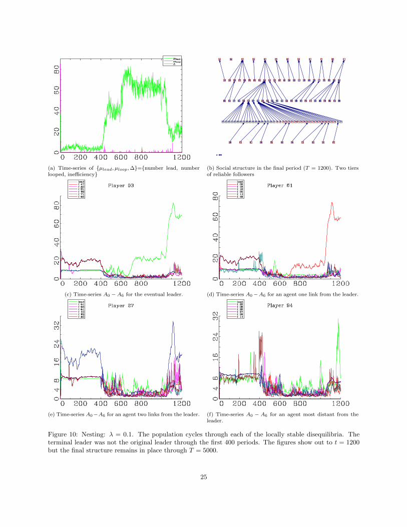
(a) Time-series of {µlead, µloop,∆}={number lead, numberlooped, inefficiency}

(b) Social structure in the final period (T = 1200). Two tiersof reliable followers



Figure 10: Nesting: λ = 0.1. The population cycles through each of the locally stable disequilibria. Theterminal leader was not the original leader through the first 400 periods. The figures show out to t = 1200but the final structure remains in place through T = 5000.

25


(b) Social structure in the final period (T = 500). One tier ofreliable followers


(e) Time-series A0−A6 for an agent two links from the leader. (f) Time-series A0 − A6 for an agent otherwise 3 links fromleader.

Figure 11: Predisposition to lead: A0,0 = 3.5 The initial bias produces h

26

3.2.8 Locally stable disequilibrium

In simulation, populations spend considerable durations within a small number of apparently stable disequi-

librium states. The time-series in 10a shows a population cycling through a number of locally stable states

of disequilibrium. Figure 12 shows example structures sampled from each state. The explanation for the

locally stable states of disequilibrium comes from considering stable social organizations in which some or

all of the population employ a mixed strategy.

Consider a homogeneous population employing a mixed strategy in which the probability of leading is

ρi = ρ and wi,j = (1 − ρ)/nd ∀i, j ∈ Ndi . This describes the behavior generating the structure observed in

Figure 12a. In each period a randomly determined portion ρ of the population leads while (1 − ρ) follows,

generating no real social organization. This behavior generates expected payoffs,6

πel (ρ) = E(πl(ρ)) = (aJ + (1− ρ)aT )n

m(9)

πef (ρ) = E(πf ) = aJn

m. (10)

Recall that, for φh < 1 or φh = 1 and κh = 1, h = l, f , the performance measure reaches a steady state

as indicated in (8). Let αh = (1−φh(1−κh))/(1−φh). The mixed strategy fixed point is the ρ∗0 that solves,

based on the nested logit condition in (4),

ρ =eµαlπ

el (ρ)

eµαlπel (ρ) + nλde

µαfπef (ρ)

. (11)

Since πel 6= πef , the mixed-strategy fixed point is not an equilibrium. The superior performance to leading

ensures that leading receives more than an equal share of the probability mass.

The other stable disequilibrium structures depicted in Figure 12 involve heterogeneous behavior made

up of four position types. These are

1. {i}: a leader, with ρi = 1,

2. ND(i) = {j ∈ N |dj,i = D}: a population of mixing agents with ρD ∈ (0, 1) who, when they follow, are

at distance D from the leader,

3. NR(i,D) = {j ∈ N\{i}|dj,i < D}: a population of reliable followers, with ρR = 0, for all j ∈ N\{i}

capable of dj,i < D, and

6For computation convenience, assume that all followers link with someone who leads in the period. This is not necessarilytrue as the chosen contact may have also chosen to follow. As a consequence, the actual expected payoff to following is higherthan indicated by this formula.

27

(a) t = 650, homogeneous population of mixing agents. (b) t = 810, mixing at distance D = 2.

(c) t = 510, mixing at distance D = 3. Leader has few directfollowers.

(d) t = 1200, mixing at distance D = 3. leader with manydirect followers.

(e) t = 200, mixing at distance 4 (bottom tier). (f) t = 1 Random action

Figure 12: Equilibrium and disequilibrium structures from the simulation producing Figure 10.

28

4. N l(i,D) = {j ∈ Ndj,i > D}: a population that leads, with ρl = 1, for all l ∈ N incapable of dj,i ≤ D.

Let nD, nR, and nl represent, respectively, the size of the ND(i), NR(i,D), and N l(i,D) populations.

For those employing the mixed strategy,

E(πf (ρ,D)) = aJ(1 + nR + (1− ρ)(nD − 1) +1

m(ρ(nD − 1) + nl)) (12)

E(πl(ρ,D)) =1

m(aJ(n− 1) + aT (nR + (1− ρ)(nD − 1)). (13)

Let

C = θ − nR + (1− ρ)(nD − 1)

1 + nR + (1− ρ)(nD − 1).

The condition C ≥ 0 implies E(πf (ρ,D) − πl(ρ,D)) ≥ 0. Since nR + (1 − ρ)(nD − 1) < n − 1, B > 0

implies C > 0 for all ρ. Thus, there is no value of ρ that will produce E(πf (ρ,D) − πl(ρ,D)) = 0. In

addition, the fixed point assigns greater probability mass on following relative to the probabilities produced

by indifference.

Let ρ∗D indicate the value of (11) evaluated at expected payoffs (12) and (13). The condition indicates that

the profit differential between the ρ∗D-dependent lead and follow payoffs for the ND(i) population support

the ρ∗D probability to lead.

To sustain the structure, the mixing population must support the pure strategy behavior of the other

agents. In particular, the (1 − ρ∗D)nD averaged sized population following at distance D has to provide

enough of a preemption payoff to the D − 1 distance followers such that ρR = 0. Transitions to a smaller

hierarchy are likely the result of small realized populations at distance D offering insufficient reward, leading

the D − 1 distance followers to mix. Similarly, as ρ∗D → 0, the agents in the N l population have reasonably

reliable connections to the leader, making following sufficiently attractive to start mixing. Transitions to a

larger hierarchy are likely the result of persistent following on the part of the ND(i) population such that

they attract their own followers. Following becomes more attractive to everyone in the ND(i) population as

the D + 1 tier fills in.

Table 2 identifies numerically derived ρ∗D values based on the parameters of Treatment 1. Using a

symmetric network of nd each of inlinks and outlinks for each agent, then nD = min{nDd , n− 1− nR}. For

nd = 6 and n = 100, the maximum distance possible is three links. The large N l(i, 2) population unable to

link to the leader contributes to the large number of agents who lead in the D = 2 mixing state.

29

Table 2: Mixing behavior and resulting social structure. Numerical solutions based on a symmetric contactnetwork using parameters from Treatment 1. Also based on each agent at distance D having only one contactat the D − 1 distance.

Mixing distance nR E(µlead) ρ∗D0/1 0 67 0.672 6 72 0.403 36 12 0.32

3.2.9 Strong desire to lead (B < 0)

A decrease in θ = (m−1) aJaT such that B < 0 changes the incentives to the most distant followers. Decreasing

m improves the likelihood that leading will produce a match with the dominant leader, increasing the

expected payoff to the strategy. A decrease in aJaT

increases the relative premium reward to leading. Both

changes increase the incentive to lead, and for B < 0 the incentive is enough to induce the most distant

followers of the dominant leader into leading.

The B < 0 equilibrium structure, with a hierarchy of size ns < 1−n followers, is potentially more difficult

to achieve. With an interior n∗s there is always some agents on the margin between leading and following. An

additional frailty arrises from the property that, to remain an attractor, for B < 0 the equilibrium structure

requires the presence of only one leader. In the presence of multiple leaders, autarky is the attractor with

the most distant followers in each hierarchy preferring to lead.7

Simulations of Treatment 10, with B = −0.055, produced ns ≥ 50 in 100% of the treatments despite an

n∗s = 15. An examination of the simulation output suggests roughly equal performance between the lead

and follow options. The simulations identify the existence of an mixed strategy equilibrium that is Pareto

improving to the pure strategy equilibrium supporting ns = n∗s.

Let di represent the maximum distance from leader i for σ ∈ Σ∗, di = maxj∈NS(i) di,j . Follower j with

dj,i,t = di can increase her distance (employing an inefficient link), increasing the payoff to any other follower

at distance di,t without lowering her own payoff. Whether at di or di + 1, she is the most distant follower,

receiving only the conformity reward. Relative to the efficient structure, there is no loss. When all agents at

di employ a non-zero probability of locating themselves at distance di + 1, the cost of realizing the greater

distance is the lost opportunity to benefit from the other players who have also increased their distance.

There is a locally stable fixed point at which each of the distance-di followers employs a non-zero proba-

bility of increasing her distance. The same is true for each tier when it is the most distant of the followers.

The practice of mixing by the most distant followers increases the payoff to the entire cohort sufficiently to

7see Goldbaum (2016).

30

exceed the payoff to leading. Their membership in the hierarchy supports the membership of all the agents

above them. The mixing behavior is evident in the inefficiency recorded in Figure 13a.

For B > 0, the pure strategy equilibrium is superior to the mixed strategy disequilibrium. Everyone,

including the most distant follower, is better off receiving the certain conformity reward inherent in the

equilibrium structure. For B < 0, the mixing is Pareto improving over the pure strategy equilibrium as the

mixing support a larger hierarchy generating greater conformity and more opportunities to preempt others.

A tendency to lock-in, introduced in Treatment 11, can disrupt the mixed-strategy equilibrium. It

magnifies performance differentiation, creating greater consistency in the relative positioning and decreases

the number who employ an inefficient link within the hierarchy. The frequencies reported for Treatment

11 reveal that a still large number of runs remain at the mixed strategy equilibrium. Those that disperse

typically end either near the equilibrium structure, as is the case in Figure 14, or reach the homogeneous

mixing disequilibrium.

3.3 Leadership Characteristics

3.3.1 Social advantage

Visibility should impact on the evolutionary process. A randomly generated contact network produces a

non-degenerative distribution of incoming links for each agent. Let ei be the number of contact links,

captured in g, directed at agent i. As revealed in Figure 15, those with a greater number of incoming links

experience a heightened probability for emerging as a leader. The two figures are each the product of 5,000

simulation iterations. In each figure, the solid (blue) curve is the distribution over the entire population of

500,000 agents as initiated at the start of the treatment. The long-dashed (red) curve is the distribution

of inlinks among the ex post population of dominant leaders as realized at the end of each iteration. The

short-dashed (black) curve is the conditional probability of emerging as a leader based on the agent’s ei.

The two treatments employ different behavior parameters but the same randomly generated 5,000 networks

of contacts upon which to consider behavior.

The treatment presented in Figure 15a employs the baseline parameters. Recalling Figure 2a, the con-

siderable heterogeneity in realized payoffs in the first period facilitates quick identification and emergence of

the equilibrium structure, typically in fewer than five periods. The random realization of potentially long

following chains generates vastly different payoffs in the first round that are quickly incorporated into an

imitation network. Advantage comes from the greater visibility and the greater chance of having followers

in that first period.

31





Figure 13: Strong lead: B = −0.055 and n∗s = 15. In large conformity populations, the attraction to lead isgreater than that of conformity.

32





Figure 14: Strong lead with lock-in: B = −0.055, κ = 0.2 Lock-in disrupts the mixed-strategy equilibriumsupporting a ns > n∗s structure by increasing discernability, to the population’s detriment.

33

(a) Leader in-link distribution under quick identification andemergence

(b) Leader in-link distribution under slow identification andemergence

Figure 15: Distribution of ei among the general agent population (solid blue) and among dominant leaders(long-dashed red). The conditional probability of leading (short-dashed black) increases in ei.

Table 3: Probability of becoming leader (5,000 iterations). Std err in parenthesis.

Treatment ei eleaders Pr(leader) βinlink instances leader—ei = 1 rel. freq. leader—ei ≥ 17

Quick 6 7.4 0.01 0.0026∗ 4 of 6655 0.069(5.95e− 5)

Slow 6 8.7 0.01 0.0048∗ 0 of 6655 0.172(5.92e− 5)

∗ Significance at the 1% level.

The treatment presented in Figure 15b sets A0,0 = 35, ensuring that every agent leads in the first period.

The in-links, thus, have no impact on first period payoffs. In addition, the IOC parameter is reduced to

µ = 0.2 to slow down the evolutionary process. With ρi,0 = 1 there is no advantage to be gained from the

initial structure. All advantage arises out of the greater visibility as individuals develop preferences based

on experience and observation. Apparently, the slower building of a reputation enhances the advantage of

visibility.

Table 3 reports indicative statistics for the two treatments. The reported βinlink is the coefficient on a

simple OLS projection of whether agent i led on the number of inlinks in excess of six. The unconditional

probability of leading is also the regression intercept. Notice that, at least for the quick treatment, visibility

does not completely dominate luck as even an agent with only one observer can still emerge as leader (for

the slow treatment, nine of 21,124 agents with only two observers emerge as leader).

34

Table 4: The population is distributed over a symmetric network in which each agent has nd = 6 outwarddirected links and nd = 6 inward directed links with no overlap between in- and out-linked neighbors.Homogeneous treatment: each agent employs the same EWA and logit parameters in responding to personalexperiences. Agent 1 always leads in the alternate. The total instances as leader is the sum for the individualover the 5,000 iterations.

Agents 2 - 100Agent 1 Avg Std Min Max

Runs as the leaderHomogeneous population 46 50.04 7.18 35 68

Agent 1 always leads 605 44.39 9.79 22 64Avg. earnings

Homogeneous population 32.21 32.21 0.32 31.29 32.92Agent 1 always leads 15.88 30.76 2.11 27.35 34.26

5000 iterations, T = 100.

3.3.2 Leading behavior

A dominant leader is someone who both leads and attracts followers. The agent cannot be assured of the

latter but does have control over the former. If x is the number of times an agent becomes the leader after

q iteration runs of the simulation, then for a homogeneous population of size n on a symmetric network,

x ∼ B(q, 1/n). For 5,000 iterations and n = 100, E(x) = 50 and SD(x) = 7.04. The first row of Table 4

reports the statistics produced from 5,000 iterations.

Consider n agents distributed over a symmetric social network of which n− 1 are homogeneous in their

use of the EWA process to guide actions. Agent 1 fails to adjust, choosing to always lead. Agent 1 emerges

as the dominant leader in 605 of 5,000 iterations or just over 12% of the time. With agent 1 over-represented

in instances as the dominant leader, the distribution of the number of observations as the dominant leader

shifts down for agents 2 through 100. While agent 1 experiences great success in becoming the leader, she

suffers in terms of earnings. The foregone income from failing to follow the 88% of the time when someone

else emerges as the leader exceeds the benefit gained from the increased probability of leading.

The experience of agent 1 suggests that one can, through strategic behavior, influence the evolutionary

process and the outcome. Such behavior also impacts the other agents of the population, not just in the

lost opportunities to lead, but also through the impact agent 1’s behavior has on the structures that tend to

emerge depending on her success or failure to be leader. Those on agent 1’s contact list, and thus dependent

on agent 1 to help build a following, suffer. The six agents on agent 1’s contact list lead on average 30.7

times with the most successful leading only 33 times, well below the average of 44.8 Those who can directly

observe agent 1 benefit from the discretion to follow her when she is leader optimize on other options when

817 of 99 agents lead 33 times of less.

35

(a) Baseline: Homogeneous population with agent 1 updat-ing behavior based on experiences

(b) Treatment: Agent 1 always leads, all others update prob-abilities according to the EWA.

Figure 16: Distribution of per-period individual earnings (5,000 iterations). The population is distributedover a symmetric directed network with no two agents able to directly observe each other. The behaviorincreases the probability that agent 1 emerges as the dominant leader of the simulation but lowers agent 1’sexpected earnings. The distribution of earning for agents 2 - 100 increases in variance relative to the base.

she does not. The average mean earning among those observing agent 1 is 33.8 with the lowest observed

mean earnings at 33.3, well above the average of 27.9 Figure 16 presents the distribution of the per period

average earning by each agent.

The diminished average earnings experience by agent 1 reflect, in part, her continuing to lead after the

entire population has formed a hierarchy under another agent. It is possible that agent 1 can profitably persist

in leading until such point that doing so is no longer advantageous. Such a strategy can be approximated by

incrementally increasing an individual’s A0,0(i), the starting value for the lead performance measure. With

A0,0(j) = 35, j ∈ {2, . . . , 100}, Figure 17 reveals a rise and then fall in agent 1’s average earning relative

to that of the population as A0,0(1) increases. From a below average earning with A0,0(1) = 1, agent 1’s

average earnings increase as she more persistently pursues the lead strategy. Agent 1’s average earnings is

observed above the 95 percentile of the population at A0,0(1) = 150 and peaks at A0,0(1) = 250 with the

highest average earnings.

3.4 Contact Selection

Allowing individuals in the population to replace low performing contacts with new contacts and the hierarchy

collapses the vertical tree structure as followers find more direct imitation paths to the leader. Eventually

a nearly completely horizontal structure emerges with the entire follower population directly imitating the

933.3 is the 18th highest mean earning of agents 2 - 100.

36

Figure 17: B = 1.21, µ = 0.2, λ = 0.8, φl = φf = 0.9, κl = κf = 0, δl = 0.9, δf = 1, A0,0(i 6= 1) = 35,T = 100, 1,000 iterations for each A0,0(1). Average earning of agent 1 relative to the population as agent 1increases persistence in leading. Population mean average earning and 10% bands shown. Also the maximumaverage earnings excluding agent 1.

dominant leader . The payoff to the leader is unchanged. The same is true for those who were most distant

from the dominant leader according to the initial contact structure. Those agents originally at intermediate

distances from the leader see their payoff diminished by the collapse of the vertical structure as they lose

their distance advantage over others in the population.

The simulation producing Figure 18 allows individuals to drop the lowest performing contacts with

wji,t < wi with wi = .5(1 − ρi)/d. Under this criterion, the contact is dropped if he or she substantially

underperforms with a probability weight that is only 50% of the average for all contacts.

4 Conclusion

When the consumers are more concerned with the social phenomenon of a product than with the product

itself, a leader plays a vital role in coordinating the population. Individuals have an interest in their position

in the social structure when leading the population earns a premium reward. Despite the inherent inequality

in the outcome, simulations indicate that a population can, when employing an appropriate mechanism of

adjustment, organize itself into the equilibrium social structure that benefits all. The self-serving but myopic

adaptive behavior produced by the experience weighted attractor (EWA) generates the needed adjustments

in individual behavior that places the larger population into the role of follower behind a single emergent

leader. That the emergence takes place with individuals unaware of the larger social structure addresses the

37



(c) Time-series A0 −A6 for the eventual leader. (d) Time-series A0 − A6 for an agent initially one link fromthe leader.

(e) Time-series A0 − A6 for an agent initially two links fromthe leader.

(f) Time-series A0 −A6 for an agent who leads in T .

Figure 18: With the ability to unilaterally and costlessly establish new potential imitation links, agentseventually find a direct link to the dominant leader. With small but non-zero probability, each followerfollows someone other than the leader such that there is typically a thinly populated second tier.

38

Kirman et al. (2007) criticism that endogenous network models tend to require unreasonably high knowledge

regarding the full social network.

The failure in the population to organize under low intensity of choice conditions or when agents down-

weight the performance signal of untried strategies points to the key elements necessary for structure to

emerge. Outcomes early in the simulation are primarily driven by random events. In the absence of any

accommodation to these early random events, they become transitory, subsumed by different randomized

outcomes in the following period. Emergence of order requires adaptation that transforms early transitory

outcomes into permanent components of a social structure. When agent i is initially lucky in selecting an

option that is popular, this attracts the attention of those who can observe agent i, increasing their likelihood

of imitating i and thereby increasing the likelihood of a positive outcome for i in subsequent periods. Agent

i’s success builds over time as the social structure adapts to, and thereby reinforces, her success.

The simulations identified locally stable mixed-strategy disequilibria structures. The disequilibria are

supported by non-degenerative probability assigned to inferior choice options. The simulations also iden-

tified a Pareto improving mixed-strategy equilibrium that supports conformity enabling structures despite

incentives that, in a pure strategy setting, undermine conformity by offering a strong reward to leading.

The backward-looking adaptive accommodation by the agent to her own evolving environment, governed

by the EWA precludes the type of forward-looking strategic behavior an agent might attempt in order to

influence the formation of the social structure to her own advantage. Personally advantageous enacted

influence on the emergent social structure through forward looking strategic behavior is practiced to the

detriment of the larger population. Strategic behavior in the form of deciding how long to lead before

implementing the first follow impacts upon both individual and aggregate outcomes.

39

References

Acemoglu, D., Bimpikis, K., Ozdaglar, A. 2010. Dynamics of information exchange in endogenous social

networks. Working Paper 16410, National Bureau of Economic Research.

Acemoglu, D., Como, G., Fagnani, F., Ozdaglar, A. 2013. Opinion fluctuations and disagreement in social

networks. Mathematics of Operations Research, 38, 1–27.

Ali, S. N., Kartik, N. 2012. Herding with collective preferences. Economic Theory, 51, 601–626.

Arifovic, J., Eaton, B. C., Walker, G. 2015. The coevolution of beliefs and networks. Journal of Economic

Behavior & Organization, 120, 46 – 63.

Bala, V., Goyal, S. 2000. A noncooperative model of network formation. Econometrica, 68, 1181–1229.

Banerjee, A. V. 1992. A simple-model of herd behavior. Quarterly Journal of Economics, 107, 797–817.

Blume, L. E., Durlauf, S. N. 2001. The interactions-based approach to socioeconomic behavior. In S. N.

Durlauf, H. P. Young eds. Social Dynamics, Cambridge MA, MIT Press, 15–44.

Branch, W., McGough, B. 2008. Replicator dynamics in a cobweb model with rationally heterogeneous

expectations. Journal of Economic Behavior & Organization, 65, 224–244.

Brock, W. A., Durlauf, S. N. 2001. Discrete choice with social interactions. The Review of Economic Studies,

68, 235–260.

Camerer, C., Ho, T. H. 1999. Experience-weighted attraction learning in normal form games. Econometrica,

67, 827–874.

Chang, M. H., Harrington, J. E. 2007. Innovators, imitators, and the evolving architecture of problem-solving

networks. Organization Science, 18, 648–666.

Corazzini, L., Pavesi, F., Petrovich, B., Stanca, L. 2012. Influential listeners: An experiment on persuasion

bias in social networks. European Economic Review, 56, 1276–1288.

Crawford, V. P., Haller, H. 1990. Learning how to cooperate: Optimal play in repeated coordination games.

Econometrica, 58, pp. 571–595.

DeGroot, M. H. 1974. Reaching a consensus. Journal of the American Statistical Association, 69, 118–121.

40

Dutta, B., Jackson, M. O. 2000. The stability and efficiency of directed communication networks. Review of

Economic Design, 5, 251 – 272.

Ellison, G., Fudenberg, D. 1995. Word-of-mouth communication and social-learning. Quarterly Journal of

Economics, 110, 93–125.

Goldbaum, D. 2016. Conformity and influence. SSRN Working Paper 2761711.

Hausman, J., McFadden, D. 1984. Specification tests for the multinomial logit model. Econometrica: Journal

of the Econometric Society, 1219–1240.

Jackson, M. O., Wolinsky, A. 1996. A strategic model of social and economic networks. Journal of Economic

Theory, 71, 44–74.

Katz, M. L., Shapiro, C. 1985. Network externalities, competition, and compatibility. American Economic

Review, 75, 424–440.

Kirman, A., Ricciotti, R. F., Topol, R. L. 2007. Bubbles in foreign exchange markets. Macroeconomic

Dynamics, 11, 102–123.

Schelling, T. C. 1971. Dynamic models of segregation. Journal of Mathematical Sociology, 1, 143–186.

Schelling, T. C. 1973. Hockey helmets, concealed weapons, and daylight savings - study of binary choices

with externalities. Journal of Conflict Resolution, 17, 381–428.

Watts, A. 2001. A dynamic model of network formation. Games and Economic Behavior, 34, 331–341.

41

Documents

Networks formation to assist decision making · Networks formation to assist decision making David Goldbaum ... [email protected] 1. ... (2010) injects a time