NETWORK OPTIMISATION

BME FACULTY OF TRANSPORTATION ENGINEERING AND VEHICLE ENGINEERING32708-2/2017/INTFIN COURSE MATERIAL SUPPORTED BY EMMI

Dr. Tibor SIPOS Ph.D.Dr. Árpád TÖRÖK Ph.D.Zsombor SZABÓ2019

NETWORK OPTIMISATION

2

Content

Minimum Cost Flow Problem

Maximum Flow Problem

Shortest Route Problem

Graph Theory

3

• Network: bunch of nodes and arcs

• Node: where the arcs intersect each other

• Arc: the nodes are connected by arcs

• In transportation sciences, the networks oftenhave some kind of flow on the arcs

• Directed arc: the flow on the arc can be in onlyone direction

• Directed network: all of the arcs are directed

Graph theory

4

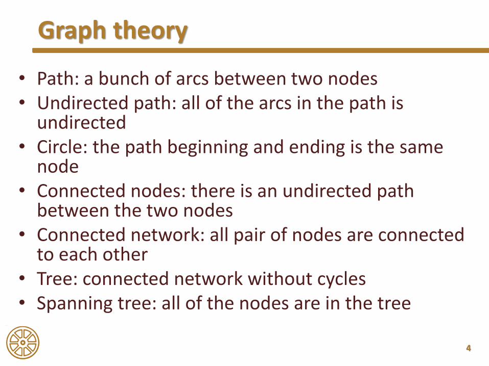
• Path: a bunch of arcs between two nodes• Undirected path: all of the arcs in the path is

undirected• Circle: the path beginning and ending is the same

node• Connected nodes: there is an undirected path

between the two nodes• Connected network: all pair of nodes are connected

to each other• Tree: connected network without cycles• Spanning tree: all of the nodes are in the tree

Graph theory

5

Content




Graph Theory

6

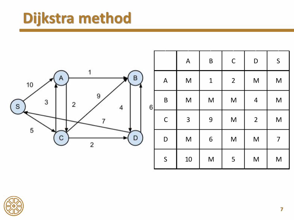
• Goal: find a minimal spanning tree, where thereis a starting point chosen arbitrary, and the othernodes distances are calculated from this point

• Theorem: a spanning tree with 𝑛 nodes has always 𝑛 − 1 arcs

• All of the networks can describe in graph and table form also

Dijkstra method

7

Dijkstra method

S 10 M 5 M M

D M 6 M M 7

C 3 9 M 2 M

B M M M 4 M

A M 1 2 M M

A B C D S

8

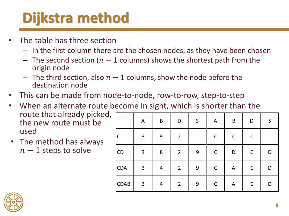
• The table has three section– In the first column there are the chosen nodes, as they have been chosen– The second section (𝑛 − 1 columns) shows the shortest path from the

origin node– The third section, also 𝑛 − 1 columns, show the node before the

destination node

• This can be made from node-to-node, row-to-row, step-to-step• When an alternate route become in sight, which is shorter than the

Dijkstra method

9 C A C D

9 C D C D

9 C A C D

S A B D S

C C C

3 4 2CDAB

3 4 2CDA

3 8 2CD

3 9 2C

A B Droute that already picked, the new route must be used

• The method has always 𝑛 − 1 steps to solve

9

• Consider all of the nodes which can be reached from the chosen nodes, and calculate the shortest path to them

• If the path’s length is shorter than the already counted, then the shorter path’s length must be used in the next

Dijkstra method

10

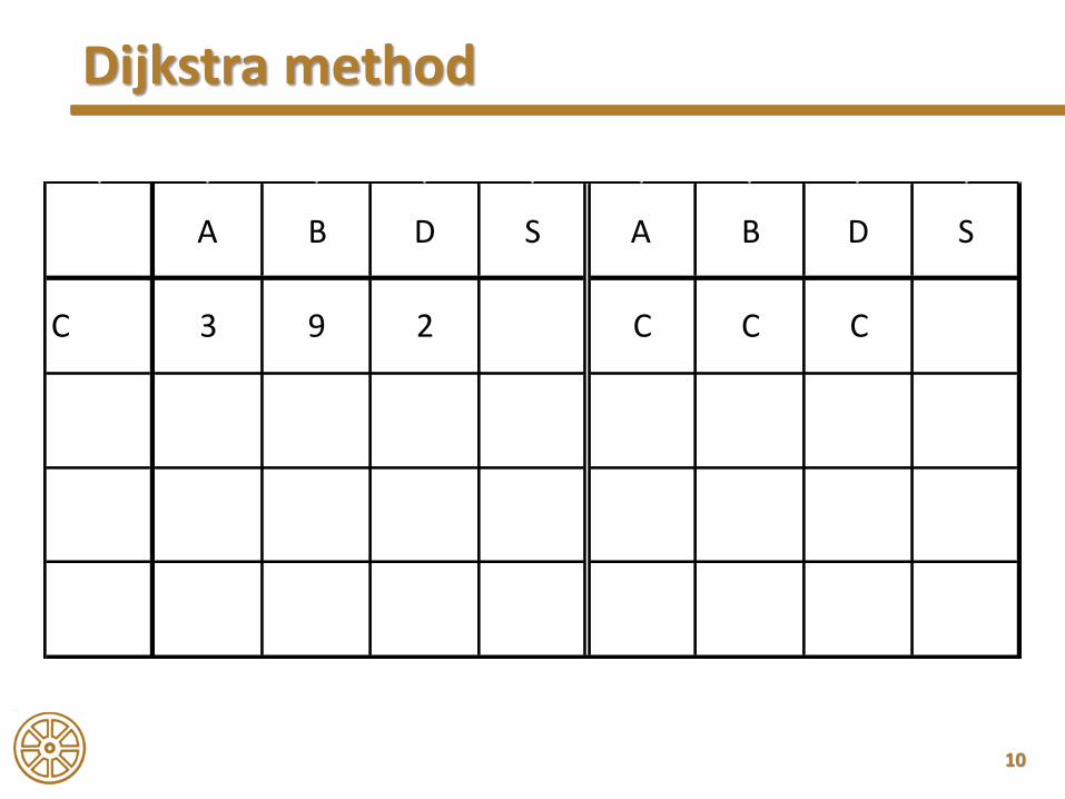
A B D S

C 3 9 2 C C C

A B D S

Dijkstra method

11

Dijkstra method

C C C

CD 3 8 2 9 C D C D

C 3 9 2

A B D S A B D S

12

Dijkstra method

C D C D

CDA 3 4 2 9 C A C D

CD 3 8 2 9

A B D S

C 3 9 2 C C C

A B D S

13

Dijkstra method

C A C D

CDAB 3 4 2 9 C A C D

CDA 3 4 2 9

C C C

CD 3 8 2 9 C D C D

C 3 9 2

A B D S A B D S

14

Content




Graph Theory

15

• Given a network

• Source: from the flows start

• Sink: flows’ destination

• Task: the most possible flows have beentransported from the source to the sink

Maximum flow problem

16

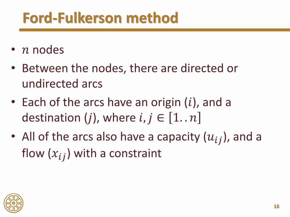
• 𝑛 nodes

• Between the nodes, there are directed orundirected arcs

• Each of the arcs have an origin (𝑖), and a destination (𝑗), where 𝑖, 𝑗 ∈ 1. . 𝑛

• All of the arcs also have a capacity (𝑢𝑖𝑗), and a

flow (𝑥𝑖𝑗) with a constraint

Ford-Fulkerson method

17

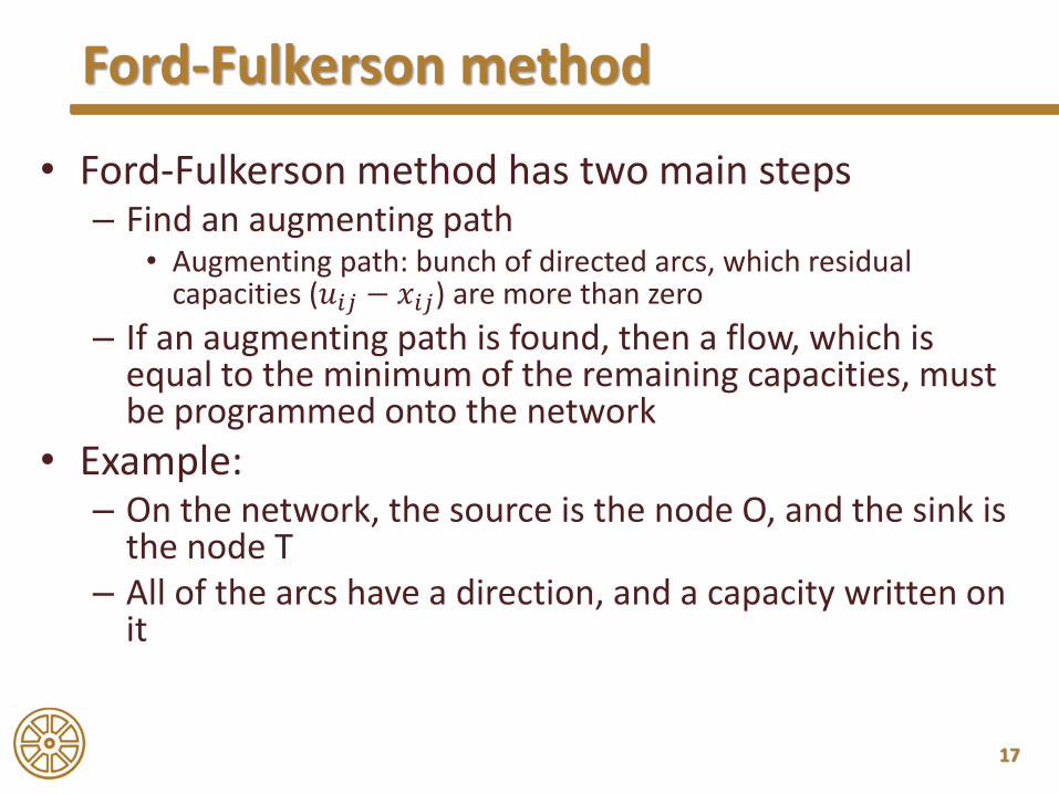
• Ford-Fulkerson method has two main steps– Find an augmenting path

• Augmenting path: bunch of directed arcs, which residualcapacities (𝑢𝑖𝑗 − 𝑥𝑖𝑗) are more than zero

– If an augmenting path is found, then a flow, which is equal to the minimum of the remaining capacities, must be programmed onto the network

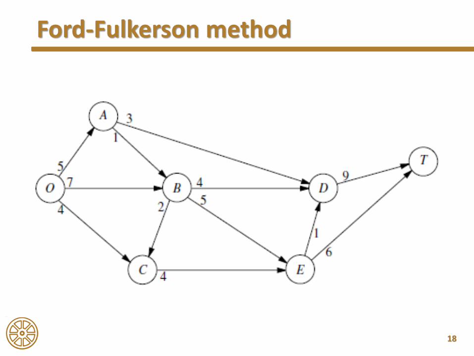
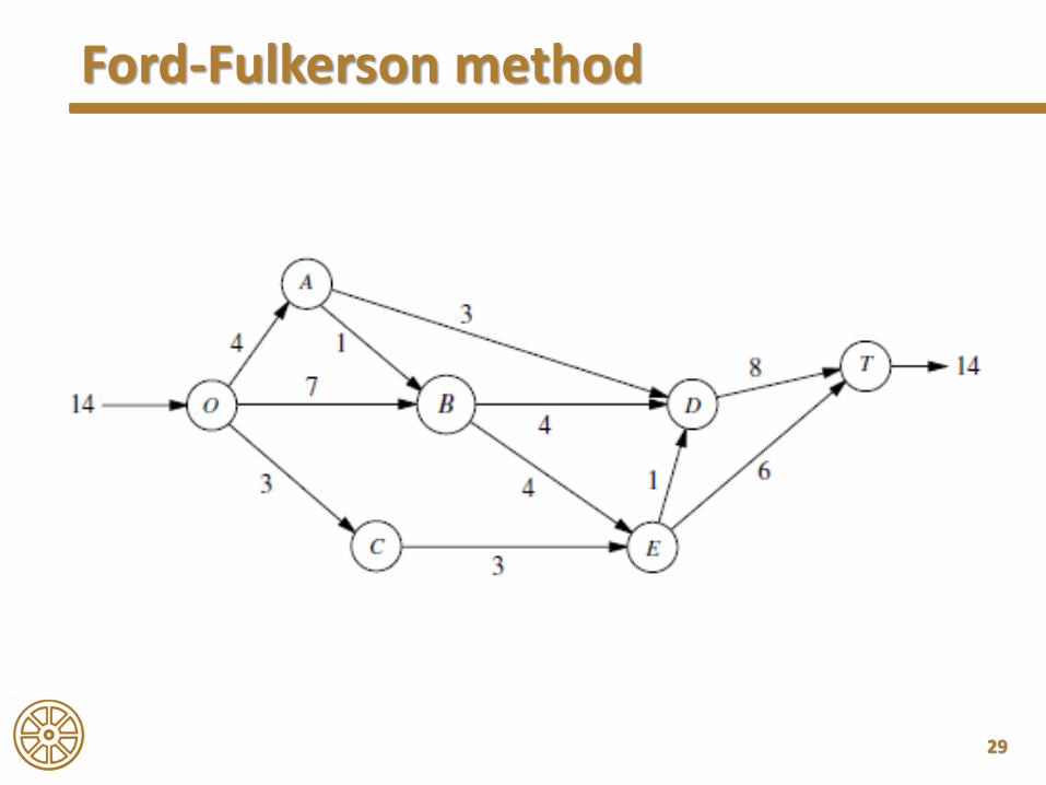
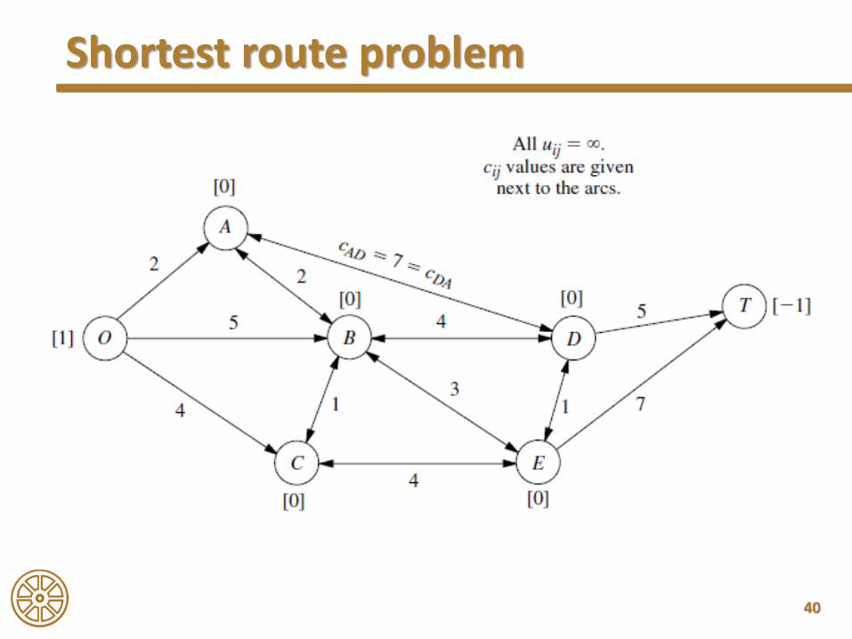
• Example:– On the network, the source is the node O, and the sink is

the node T– All of the arcs have a direction, and a capacity written on

it


18


19


20


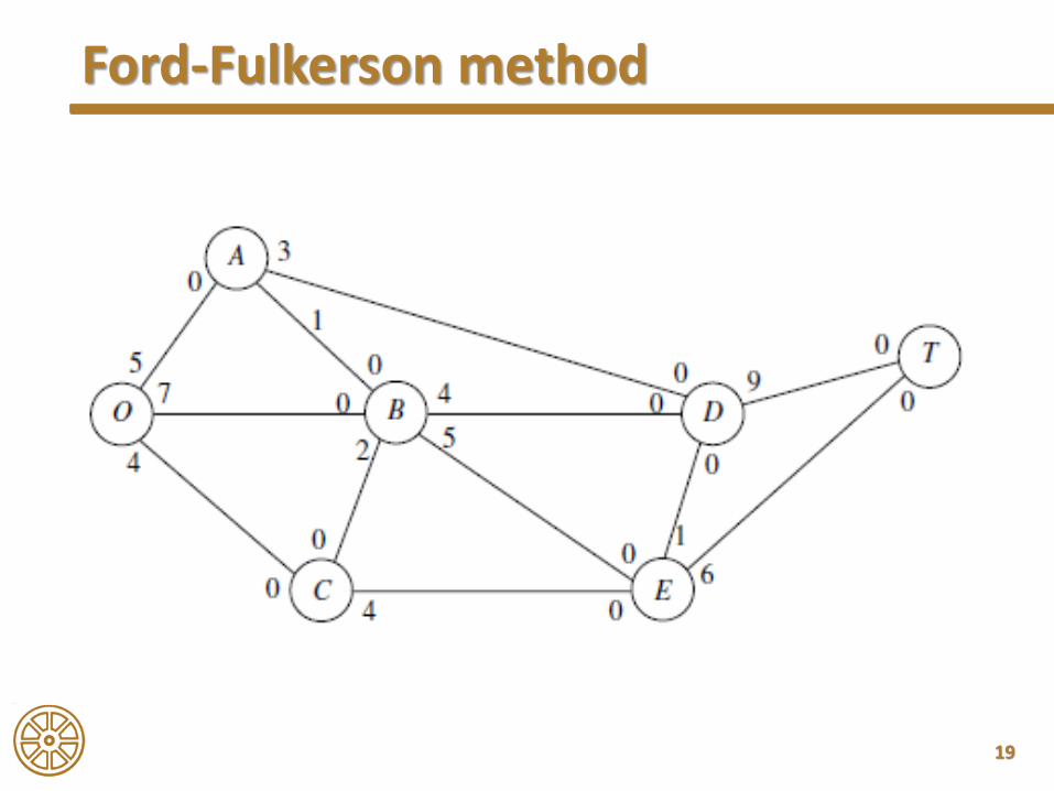
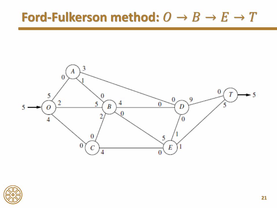
• All of the arcs have two numbers

• The first shows the residual capacity, and thesecond shows the actual flow on it

• For example, take into consideration the 𝑂 →𝐵 → 𝐸 → 𝑇 augmenting path– The minimum residual capacity is the 5 (on the BE

arc) so it can be programmed on the network

– The programmed flow must be reduce from theinvolved arcs first number, and have to add to thesecond

21

Ford-Fulkerson method: 𝑂 → 𝐵 → 𝐸 → 𝑇

22

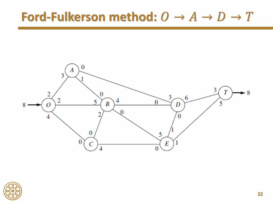
Ford-Fulkerson method: 𝑂 → 𝐴 → 𝐷 → 𝑇

23

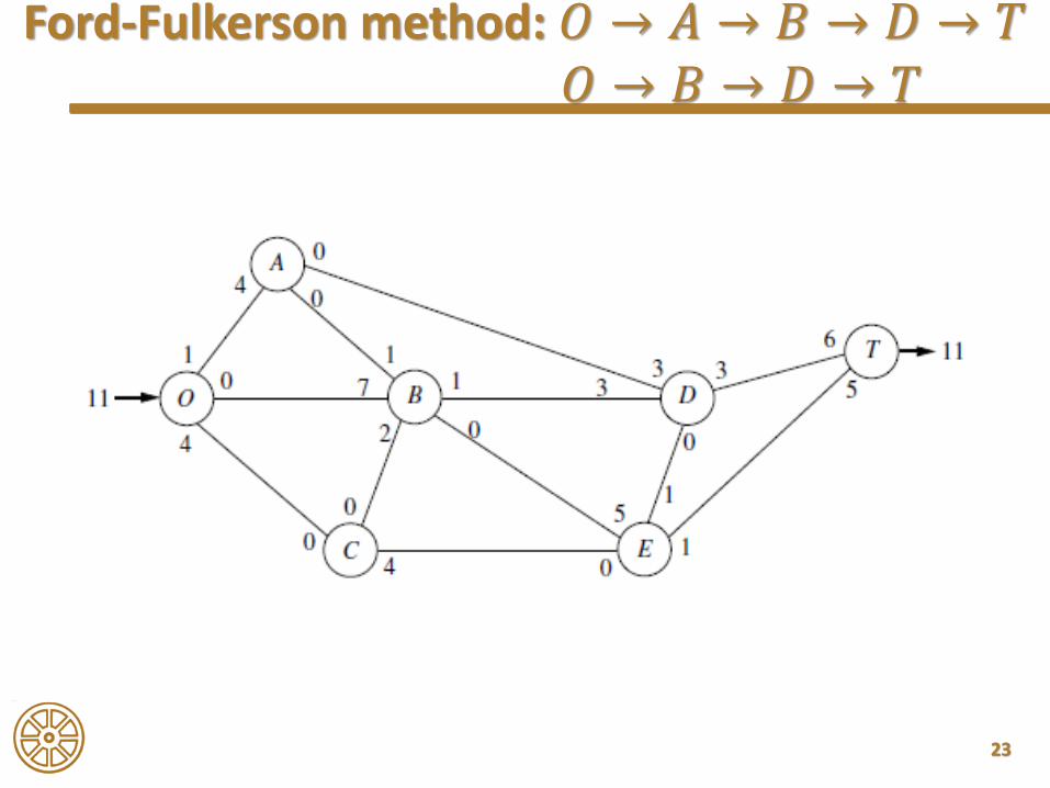
Ford-Fulkerson method: 𝑂 → 𝐴 → 𝐵 → 𝐷 → 𝑇𝑂 → 𝐵 → 𝐷 → 𝑇

24

Ford-Fulkerson method: 𝑂 → 𝐶 → 𝐸 → 𝐷 → 𝑇𝑂 → 𝐶 → 𝐸 → 𝑇

25


• Important question is, that how an augmentingpath can be found

• The method is that we start from the source and sign all of the nodes where the arc’s first number(which is closer to the already signed node) is more than zero

26


27


• Note, that in this case the BE arc’s direction is opposite

• Some unit of programmed flow can be unprogrammed, and the connecting flows must be redirected to other route

• 𝑂 → 𝐶 → 𝐸 → 𝐵 → 𝐷 → 𝑇 route can be found

28


29


30

Ford-Fulkerson method – Optimality test

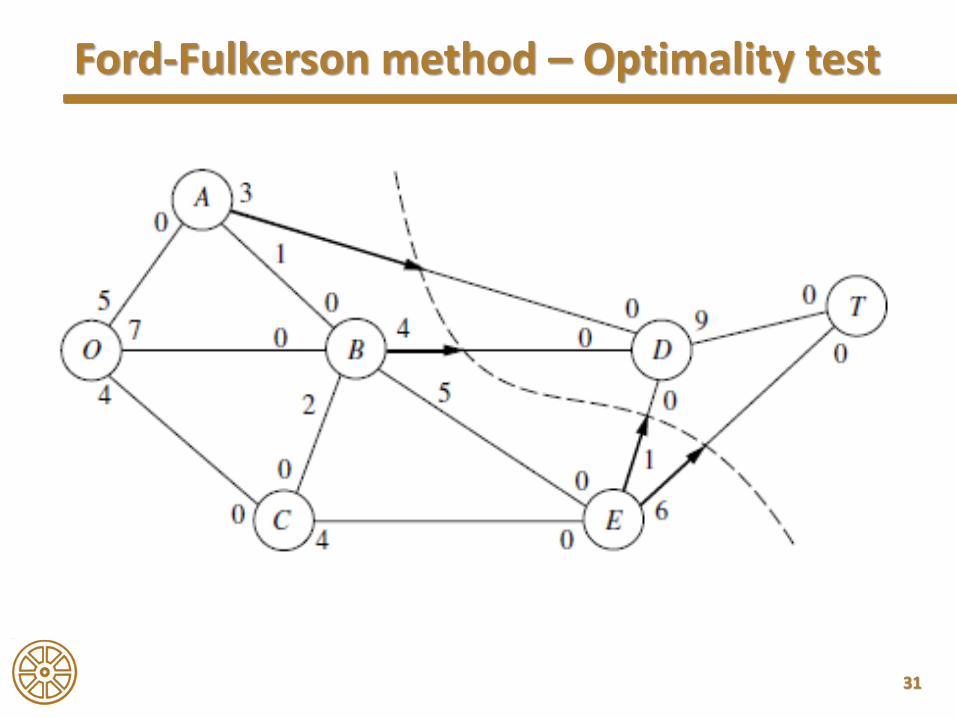
• Finding an augmenting path can be difficult in hugenetworks

• Optimality test: max-flow min-cut theorem

• Cut: any set of directed arcs containing at least one arc from every directed path from the source to the sink

• Cut value: the sum of the arc capacities of the arcs (in thespecified direction) of the cut

• Theorem: max-flow min-cut: for any network with a singlesource and sink, the maximum feasible flow from thesource to the sink equals the minimum cut value for allcuts of the network

31

Ford-Fulkerson method – Optimality test

32

Content




Graph Theory

33

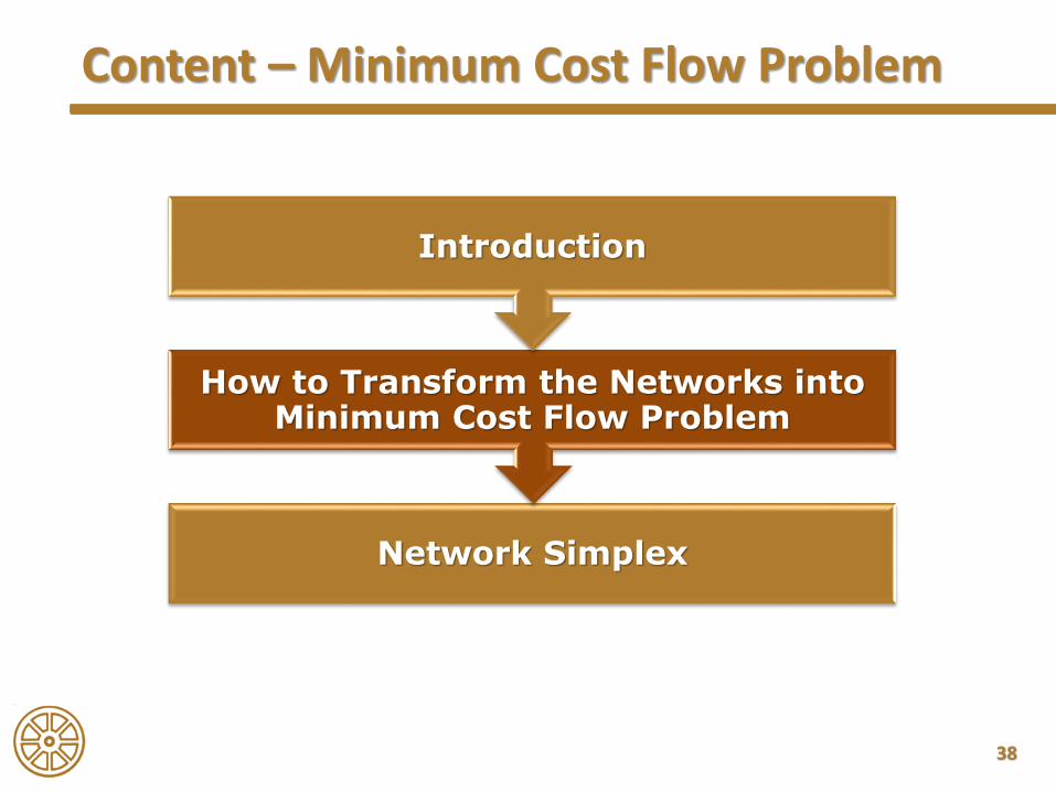
Content – Minimum Cost Flow Problem

Network Simplex

How to Transform the Networks into Minimum Cost Flow Problem

Introduction

34

• The minimum cost flow problem holds a centralposition among network optimization models, both because it encompasses such a broad classof applications and because it can be solvedextremely efficiently

• All of the previously shown problems are special cases of this problem

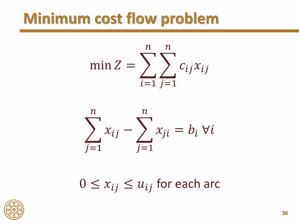
Minimum cost flow problem

35

• Have to set up two matrices– 𝑿: contains the flows, which means that the flow

between 𝑖 and 𝑗 nodes is 𝑥𝑖𝑗– 𝑪: contains the costs of the unit flows between 𝑖 and 𝑗

(𝑐𝑖𝑗)

• All of the arcs in the network have a capacity (𝑢𝑖𝑗) which means the maximum feasible flow on the arcs

• And each node has a number (𝑏𝑖), which mean thenet flow generated at node i– If 𝑏𝑖 > 0, then the node is called supply node (source)– If 𝑏𝑖 < 0, then the node is demand node (sink)


36

min𝑍 =

𝑖=1

𝑛

𝑗=1

𝑛

𝑐𝑖𝑗𝑥𝑖𝑗

𝑗=1

𝑛

𝑥𝑖𝑗 −

𝑗=1

𝑛

𝑥𝑗𝑖 = 𝑏𝑖 ∀𝑖

0 ≤ 𝑥𝑖𝑗 ≤ 𝑢𝑖𝑗 for each arc


37

Network simplex method

38


Network Simplex


Introduction

39

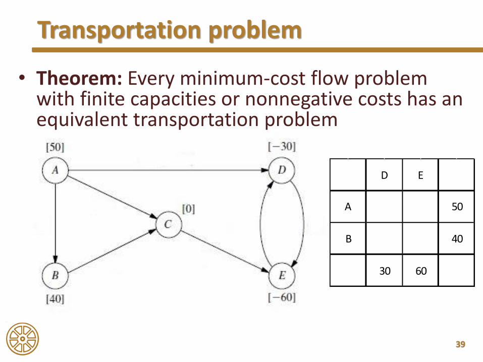
• Theorem: Every minimum-cost flow problem with finite capacities or nonnegative costs has an equivalent transportation problem

Transportation problem

30 60

B

50

40

D E

A

40

Shortest route problem

41

Maximum flow problem

42


Network Simplex


Introduction

43

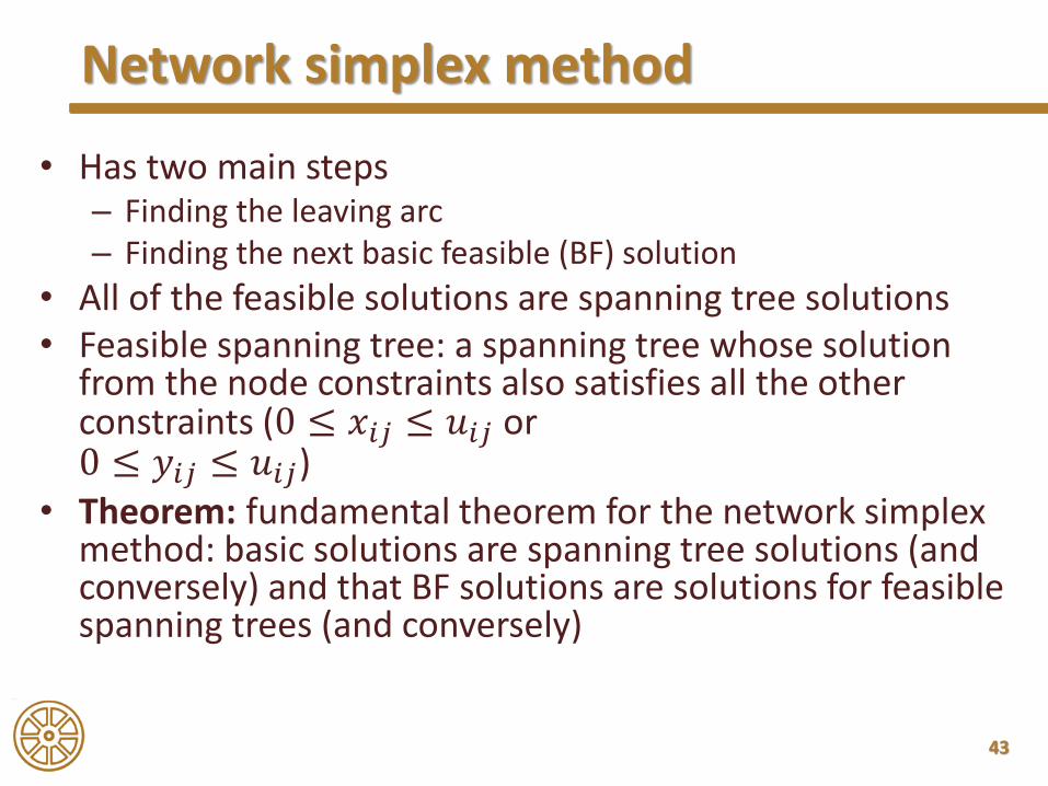
• Has two main steps– Finding the leaving arc– Finding the next basic feasible (BF) solution

• All of the feasible solutions are spanning tree solutions• Feasible spanning tree: a spanning tree whose solution

from the node constraints also satisfies all the otherconstraints (0 ≤ 𝑥𝑖𝑗 ≤ 𝑢𝑖𝑗 or0 ≤ 𝑦𝑖𝑗 ≤ 𝑢𝑖𝑗)

• Theorem: fundamental theorem for the network simplexmethod: basic solutions are spanning tree solutions (and conversely) and that BF solutions are solutions for feasiblespanning trees (and conversely)


44


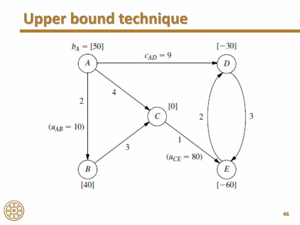
• Two arcs haveconstraints on it

– 𝑢𝐴𝐵 = 10

– 𝑢𝐶𝐸 = 80

• The cost of thearcs are the next

E 2

D 3

C 1

B 3

A 2 4 9

A B C D E𝑐𝑖𝑗

45

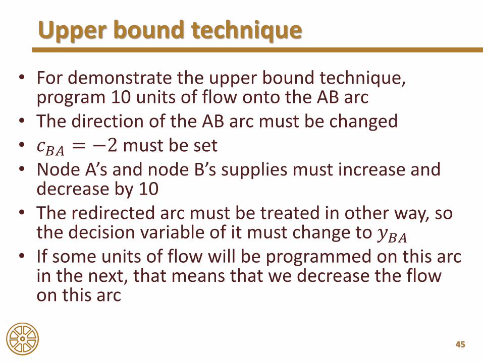
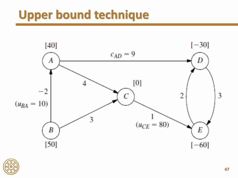
• For demonstrate the upper bound technique, program 10 units of flow onto the AB arc

• The direction of the AB arc must be changed• 𝑐𝐵𝐴 = −2 must be set• Node A’s and node B’s supplies must increase and

decrease by 10• The redirected arc must be treated in other way, so

the decision variable of it must change to 𝑦𝐵𝐴• If some units of flow will be programmed on this arc

in the next, that means that we decrease the flow on this arc

Upper bound technique

46


47


48

• An initial feasible solution is need to be set up

Initial feasible solution

49

Initial feasible solution

50

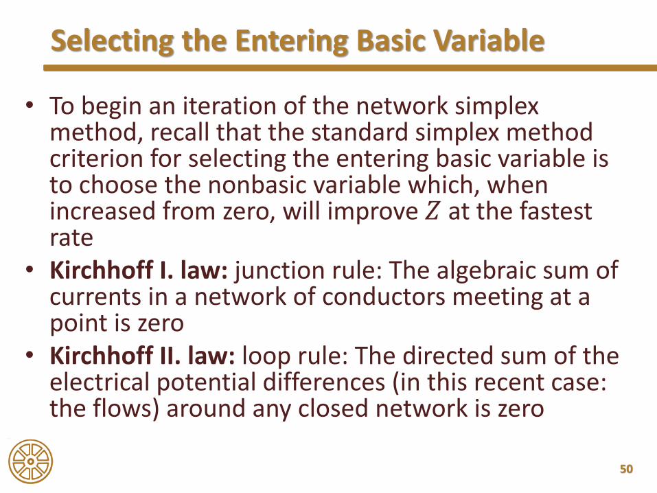
• To begin an iteration of the network simplexmethod, recall that the standard simplex methodcriterion for selecting the entering basic variable is to choose the nonbasic variable which, whenincreased from zero, will improve 𝑍 at the fastestrate

• Kirchhoff I. law: junction rule: The algebraic sum of currents in a network of conductors meeting at a point is zero

• Kirchhoff II. law: loop rule: The directed sum of theelectrical potential differences (in this recent case: the flows) around any closed network is zero

Selecting the Entering Basic Variable

51

• To choose the entering basic variable, take intoconsideration all of the nonbasic arcs

• Program on each actual arc a 𝜃 units of flow

• Then increase or decrease all of the basic arc’sflow as Kirchhoff’s second law said

• Then 𝑍 must be analysed

Selecting the Entering Basic Variable

52

∆𝑍 = 𝑐𝐴𝐶𝜃 + 𝑐𝐶𝐸𝜃 − 𝑐𝐷𝐸𝜃 − 𝑐𝐴𝐷𝜃 = 4𝜃 + 𝜃 − 3𝜃 − 9𝜃 = −7𝜃

∆𝑍 = ቐ

−7 if ∆𝑥𝐴𝐶= 16 if ∆𝑦𝐴𝐵= 15 if ∆𝑥𝐸𝐷= 1

Selecting the Entering Basic Variable – for AC arc

53

• For finding the leaving basic variable, the task is to find the maximum value of the 𝜃, where all of the arc’s constraints are satisfied

• When the flows are decreasing this bound is thenonnegativity constraint, but when the flows aredecreasing they are the capacity bounds

Finding the Leaving Basic Variable

54

𝑥𝐴𝐶 = 𝜃 ≤ ∞𝑥𝐶𝐸 = 50 + 𝜃 ≤ 80, so 𝜃 ≤ 30𝑥𝐷𝐸 = 10 − 𝜃 ≥ 0, so 𝜃 ≤ 10𝑥𝐴𝐷 = 40 − 𝜃 ≥ 0, so 𝜃 ≤ 40

• To satisfy all of the constraints the 𝜃 = 10 will be the best choice

• A nonnegativity constraint will be the bound, sothe use of the upper bound technique will nothappen in this step

Finding the Leaving Basic Variable

55

Actual Solution after the First Step

56

∆𝑍 = ቐ

7 if ∆𝑥𝐷𝐸= 1−1 if ∆𝑦𝐴𝐵= 1−2 if ∆𝑥𝐸𝐷= 1

𝑥𝐸𝐷 = 𝜃 ≤ ∞, so 𝜃 ≤ ∞𝑥𝐴𝐷 = 30 − 𝜃 ≥ 0, so 𝜃 ≤ 30𝑥𝐴𝐶 = 10 + 𝜃 ≤ ∞, so 𝜃 ≤ ∞𝑥𝐶𝐸 = 60 + 𝜃 ≤ 0, so 𝜃 ≤ 20

• Because upper bound is reached, upper boundtechnique is needed to use

2nd step

57

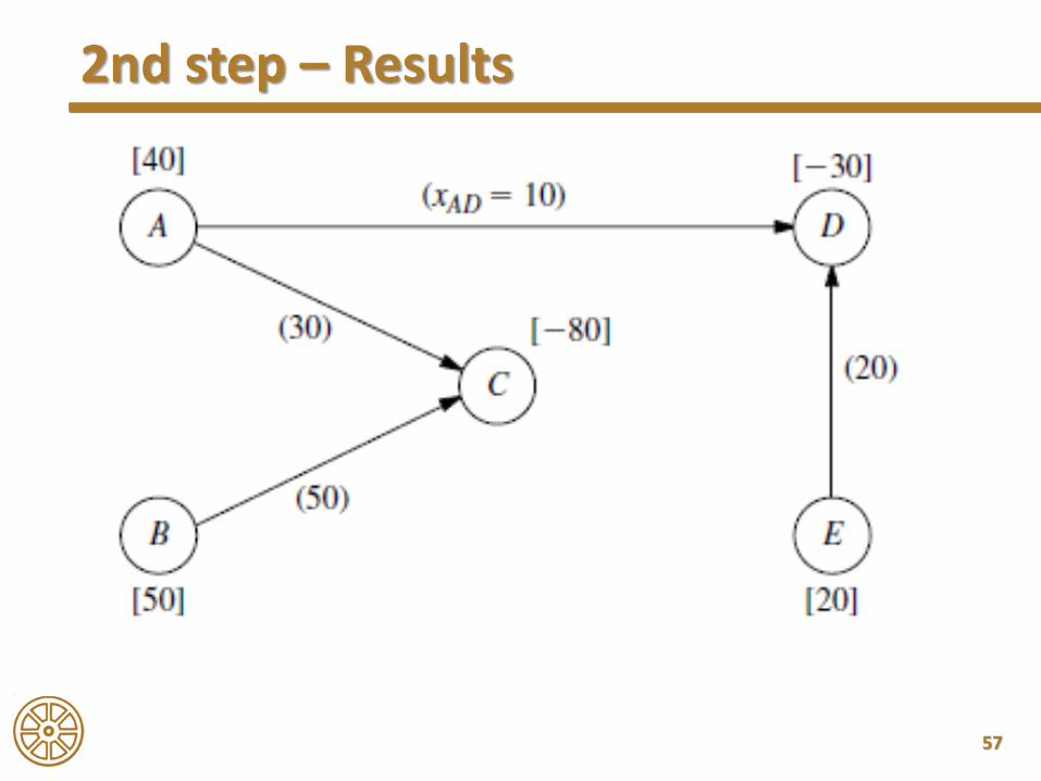
2nd step – Results

58

2nd step – Results

59

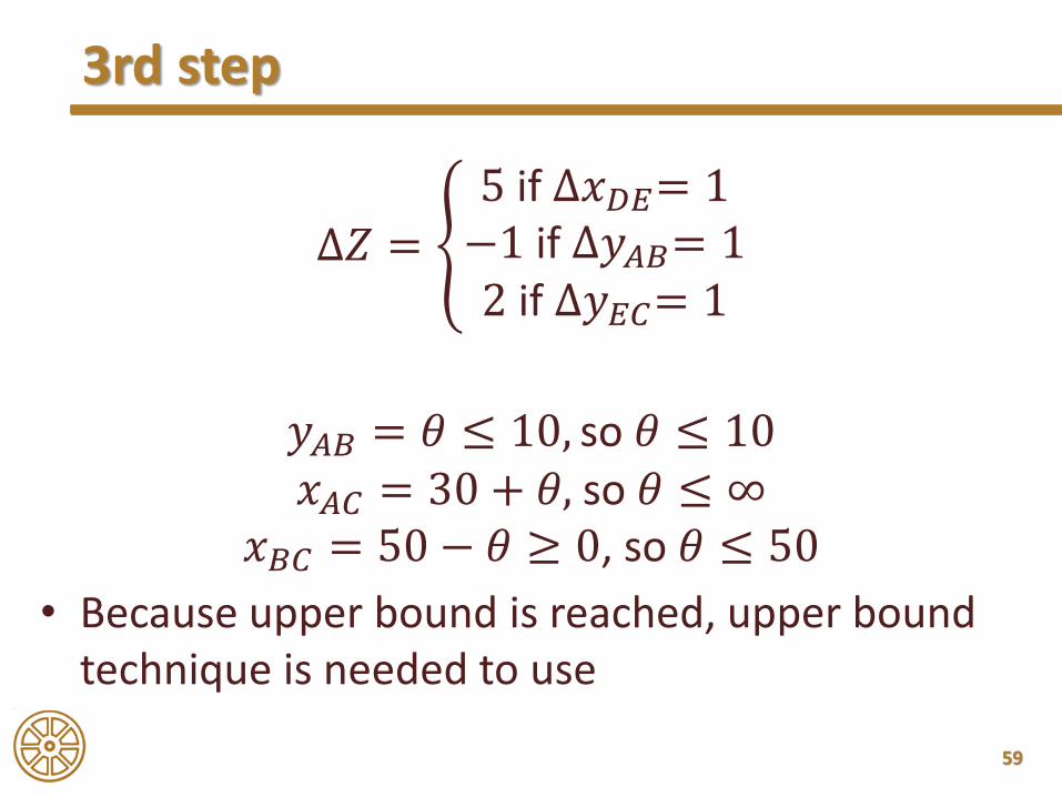
∆𝑍 = ቐ

5 if ∆𝑥𝐷𝐸= 1−1 if ∆𝑦𝐴𝐵= 12 if ∆𝑦𝐸𝐶= 1

𝑦𝐴𝐵 = 𝜃 ≤ 10, so 𝜃 ≤ 10𝑥𝐴𝐶 = 30 + 𝜃, so 𝜃 ≤ ∞

𝑥𝐵𝐶 = 50 − 𝜃 ≥ 0, so 𝜃 ≤ 50

• Because upper bound is reached, upper boundtechnique is needed to use

3rd step

60

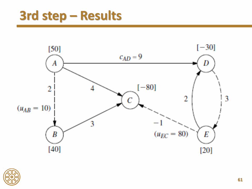
3rd step – Results

61

3rd step – Results

62

∆𝑍 = ቐ

1 if ∆𝑥𝐴𝐵= 17 if ∆𝑥𝐷𝐸= 12 if ∆𝑦𝐸𝐶= 1

• None of the new arcs decreasing the objectivefunction

• Optimal solution is reached

4th step

63

Optimal solution

64

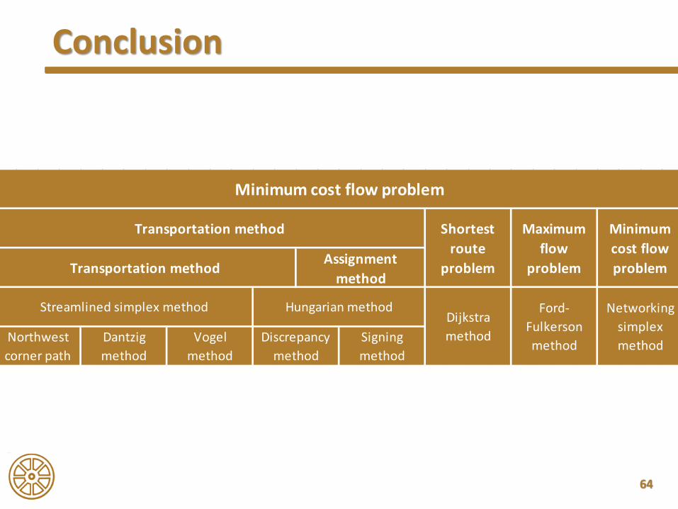
Conclusion

Minimum

cost flow

problem

Networking

simplex

method


Transportation methodAssignment

method

Transportation method Shortest

route

problem

Dijkstra

method

Maximum

flow

problem

Ford-

Fulkerson

method

Hungarian method

Discrepancy

method

Signing

method

Northwest

corner path

Dantzig

method

Vogel

method

Streamlined simplex method

BME FACULTY OF TRANSPORTATION ENGINEERING AND VEHICLE ENGINEERING32708-2/2017/INTFIN COURSE MATERIAL SUPPORTED BY EMMI

Dr. Tibor SIPOS Ph.D.Dr. Árpád TÖRÖK Ph.D.Zsombor SZABÓ

email: [email protected]

BUDAPEST UNIVERSITY OF TECHNOLOGY AND ECONOMICS

66

• Hillier F. S, Lieberman G. J. The Maximum Flow Problem. In: Hillier F. S, Lieberman G. J. Introduction to Operations Research. 7th ed. New York: McGrow-Hill; 2001. p. 420-429. ISBN: 0-07-232169-5

• Hillier F. S, Lieberman G. J. The Minimum Cost Flow Problem. In: Hillier F. S, Lieberman G. J. Introduction to Operations Research. 7th ed. New York: McGrow-Hill; 2001. p. 429-438. ISBN: 0-07-232169-5

Source of the Images, and the Example

Documents

NETWORK OPTIMISATION