Embed Size (px)
DESCRIPTION
net sim
Citation preview
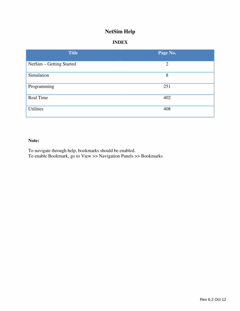
NetSim Help
INDEX
Title Page No.
NetSim – Getting Started 2
Simulation 8
Programming 251
Real Time 402
Utilities 408
Note:
To navigate through help, bookmarks should be enabled.
To enable Bookmark, go to View >> Navigation Panels >> Bookmarks
Rev 6.2 Oct 12
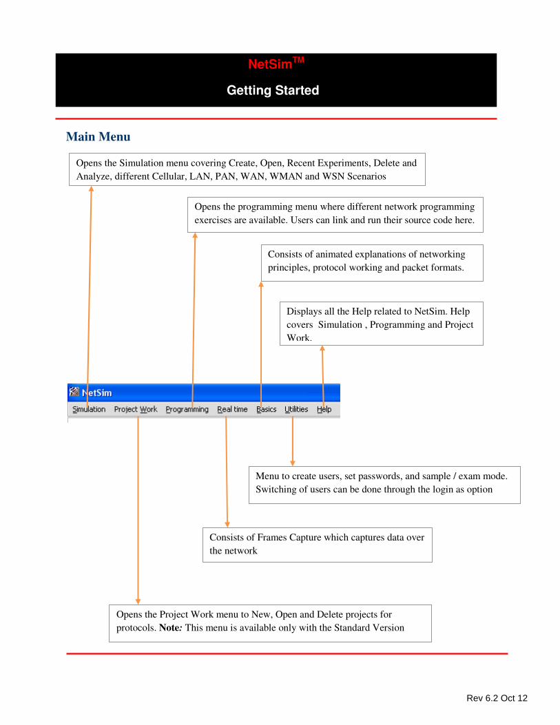
Main Menu
NetSimTM
Getting Started
Opens the Project Work menu to New, Open and Delete projects for
protocols. Note: This menu is available only with the Standard Version
Opens the programming menu where different network programming
exercises are available. Users can link and run their source code here.
Consists of animated explanations of networking
principles, protocol working and packet formats.
Menu to create users, set passwords, and sample / exam mode.
Switching of users can be done through the login as option
Displays all the Help related to NetSim. Help
covers Simulation , Programming and Project
Work.
Consists of Frames Capture which captures data over
the network
Opens the Simulation menu covering Create, Open, Recent Experiments, Delete and
Analyze, different Cellular, LAN, PAN, WAN, WMAN and WSN Scenarios
Rev 6.2 Oct 12
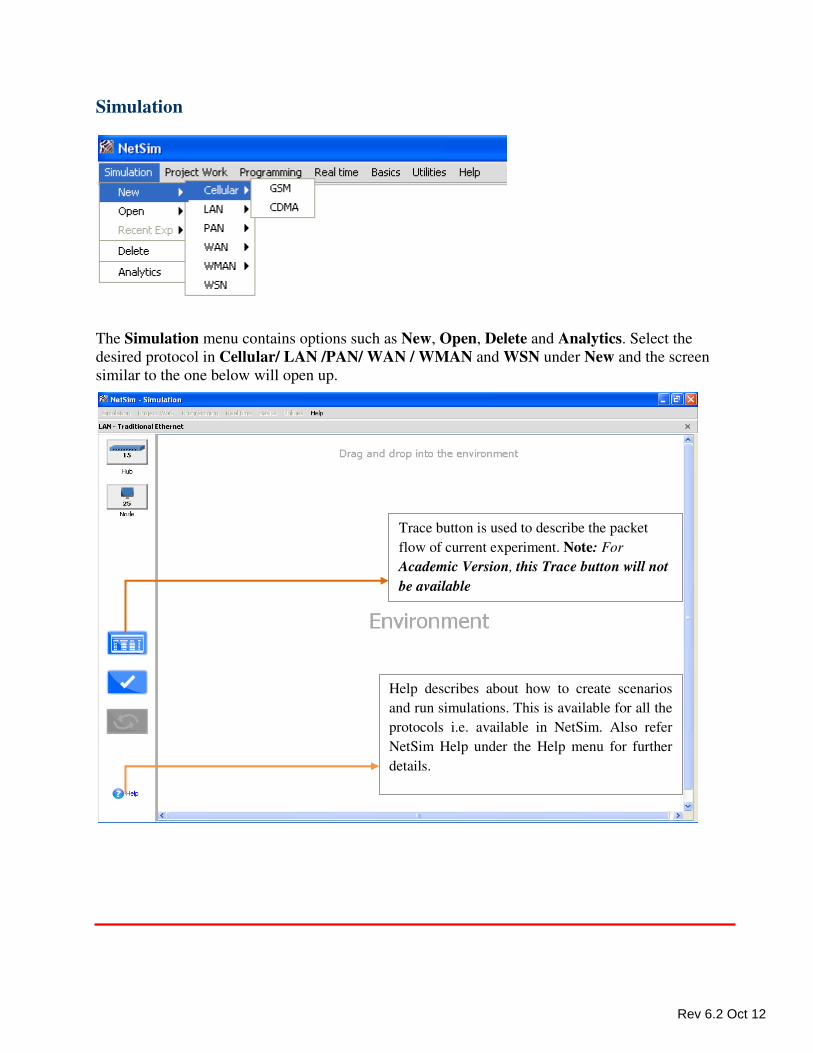
Simulation
The Simulation menu contains options such as New, Open, Delete and Analytics. Select the
desired protocol in Cellular/ LAN /PAN/ WAN / WMAN and WSN under New and the screen
similar to the one below will open up.
Help describes about how to create scenarios
and run simulations. This is available for all the
protocols i.e. available in NetSim. Also refer
NetSim Help under the Help menu for further
details.
Trace button is used to describe the packet
flow of current experiment. Note: For
Academic Version, this Trace button will not
be available
Rev 6.2 Oct 12

Project Work
Note: Project Work menu is available only with the standard version
The Project Work menu contains options such as New, Open, Delete. Select the desired
protocol from Protocol list under New and the screen similar to the one below will open up.
Clicking on the layers shows the list of primitives for that
layer Protocol lists shows the available
protocols for project work.
Selecting the list of primitives for the
project work
Rev 6.2 Oct 12
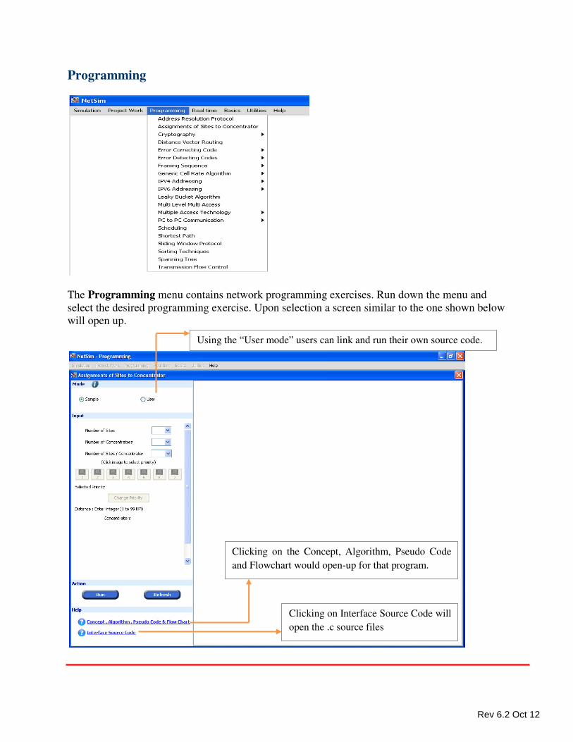
Programming
The Programming menu contains network programming exercises. Run down the menu and
select the desired programming exercise. Upon selection a screen similar to the one shown below
will open up.
Clicking on the Concept, Algorithm, Pseudo Code
and Flowchart would open-up for that program.
Using the “User mode” users can link and run their own source code.
Clicking on Interface Source Code will
open the .c source files
Rev 6.2 Oct 12
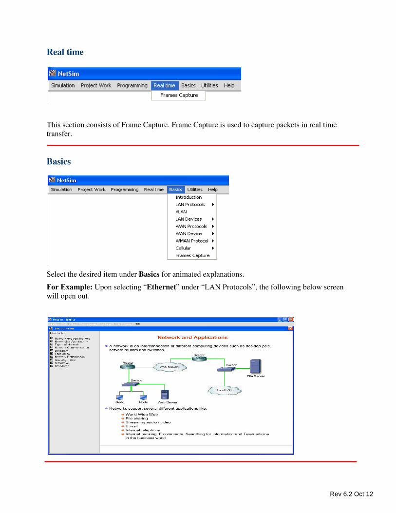
Real time
This section consists of Frame Capture. Frame Capture is used to capture packets in real time
transfer.
Basics
Select the desired item under Basics for animated explanations.
For Example: Upon selecting “Ethernet” under “LAN Protocols”, the following below screen
will open out.
Rev 6.2 Oct 12
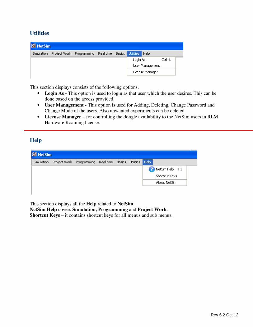
Utilities
This section displays consists of the following options,
• Login As - This option is used to login as that user which the user desires. This can be
done based on the access provided.
• User Management - This option is used for Adding, Deleting, Change Password and
Change Mode of the users. Also unwanted experiments can be deleted.
• License Manager – for controlling the dongle availability to the NetSim users in RLM
Hardware Roaming license.
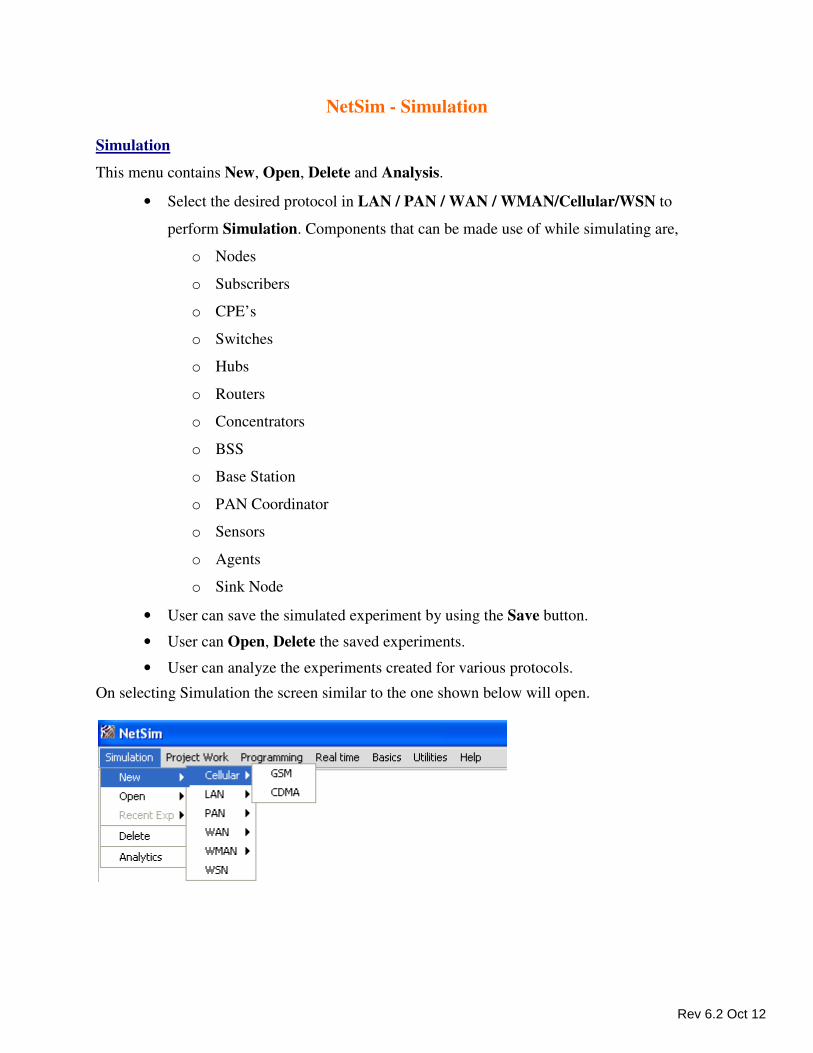
Help
This section displays all the Help related to NetSim.
NetSim Help covers Simulation, Programming and Project Work.
Shortcut Keys – it contains shortcut keys for all menus and sub menus.
Rev 6.2 Oct 12
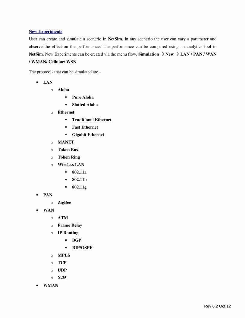
NetSim - Simulation
Simulation
This menu contains New, Open, Delete and Analysis.
• Select the desired protocol in LAN / PAN / WAN / WMAN/Cellular/WSN to
perform Simulation. Components that can be made use of while simulating are,
o Nodes
o Subscribers
o CPE’s
o Switches
o Hubs
o Routers
o Concentrators
o BSS
o Base Station
o PAN Coordinator
o Sensors
o Agents
o Sink Node
• User can save the simulated experiment by using the Save button.
• User can Open, Delete the saved experiments.
• User can analyze the experiments created for various protocols.
On selecting Simulation the screen similar to the one shown below will open.
Rev 6.2 Oct 12
New Experiments
User can create and simulate a scenario in NetSim. In any scenario the user can vary a parameter and
observe the effect on the performance. The performance can be compared using an analytics tool in
NetSim. New Experiments can be created via the menu flow, Simulation � New � LAN / PAN / WAN
/ WMAN/ Cellular/ WSN.
The protocols that can be simulated are -
• LAN
o Aloha
� Pure Aloha
� Slotted Aloha
o Ethernet
� Traditional Ethernet
� Fast Ethernet
� Gigabit Ethernet
o MANET
o Token Bus
o Token Ring
o Wireless LAN
� 802.11a
� 802.11b
� 802.11g
• PAN
o ZigBee
• WAN
o ATM
o Frame Relay
o IP Routing
� BGP
� RIP/OSPF
o MPLS
o TCP
o UDP
o X.25
• WMAN
Rev 6.2 Oct 12

o Fixed Wi-MAX
• Cellular
o CDMA
o GSM
• WSN
Rev 6.2 Oct 12
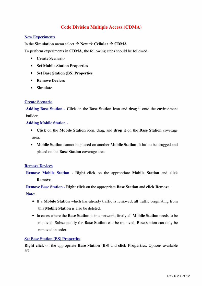
Code Division Multiple Access (CDMA)
New Experiments
In the Simulation menu select � New � Cellular � CDMA
To perform experiments in CDMA, the following steps should be followed,
• Create Scenario
• Set Mobile Station Properties
• Set Base Station (BS) Properties
• Remove Devices
• Simulate
Create Scenario
Adding Base Station - Click on the Base Station icon and drag it onto the environment
builder.
Adding Mobile Station -
• Click on the Mobile Station icon, drag, and drop it on the Base Station coverage
area.
• Mobile Station cannot be placed on another Mobile Station. It has to be dragged and
placed on the Base Station coverage area.
Remove Devices
Remove Mobile Station - Right click on the appropriate Mobile Station and click
Remove.
Remove Base Station - Right click on the appropriate Base Station and click Remove.
Note:
• If a Mobile Station which has already traffic is removed, all traffic originating from
this Mobile Station is also be deleted.
• In cases where the Base Station is in a network, firstly all Mobile Station needs to be
removed. Subsequently the Base Station can be removed. Base station can only be
removed in order.
Set Base Station (BS) Properties
Right click on the appropriate Base Station (BS) and click Properties. Options available
are,
Rev 6.2 Oct 12
Wireless Properties - Under Wireless Properties tab the options available are,
Device Type – This property defines the current device type. Base Station is set as
default.
Connected To - This property defines the Wireless medium connected to the Base
Station (BS). A default value is already entered; hence no changes can be
done.
Code Division Multiple Access
Standards – This property defines standards used to perform the CDMA simulation.
The default value is set as IS95A/B.
Total Bandwidth – This property defines the range of bandwidth that is going too used
for transmission. By default, 1.25 MHz is set as default. This value
is auto-change based on the standard type selection.
Chip Rate (in mcps) - This property specifies the chip rate of CDMA system. This
value is auto-change based on the standard type selection. By
default, 1.2288 is set for IS95A/B.
Voice Activity factor – This property defines the Voice activity for current system. This
value is always in between 0-1. By default, 0 is set default voice activity factor.
BTS Range – This property defines the range of BTS in km. The default value is set as 1
km.
Transmission Power (in W) – This property defines the transmission power used by the
current base station. 20W is set as default.
Modulation Technique – This property define the modulation technique used by the
BTS. This value is fixed at GMSK.
Multiple Access Technology – This property defines the multiple access technology
used by the CDMA system. This is fixed as Code Division Multiple Access (CDMA).
Speech Coding – This property denotes the speech coding technique used in the Base
station. This property is fixed at Linear Predictive Coding (LPC).
Target SNR - This property denotes the target SNR used for the current scenario. This
value is fixed at 6 db.
Rev 6.2 Oct 12
Channel Characteristics-
Path loss exponent – This property defines the path loss exponent of the channel used
by the current scenario. By default, this value is set as 4.
Fading Figure – This property defines the fading figure of channel used by the current
scenario. By default, this value is set as 0.5.
Standard Deviation – This value denotes the standard deviation of fading of channel
used by current scenario. By default, this value is set at 6.
Set Mobile Station Properties
Right Click on the appropriate Mobile Station to select Properties. Inside the properties
window click on Application1 to modify its properties.
Transmission Type
This indicates the type of transmission made by this Mobile station, Point to Point.
Destination
This property indicates the Destination Mobile Station.
Traffic Type
This property indicates the type of traffic. The traffic can only be Voice.
Voice
Call Details
Call Interval Time (Secs)
This property denotes the Call Interval Time. Each Call begins exponentially with mean
call inter arrival time. 300 sec is set as default Call Inter Arrival Time. User can select
450 secs or 600 secs as Call Interval Time.
Call Duration (Secs)
This property denotes how long the call continues. By default 60 secs is set as Call
duration. User can select 120 and 240 secs as their call duration value.
Codec
Codec is the component of any voice system that translates between analog speech and
the bits used to transmit them. Every codec transmits a burst of data in a packet that can
be reconstructed into voice.
Rev 6.2 Oct 12
Service Type
• CBR - CBR stands for Constant Bit Rate. Packets of constant size are generated at
constant inter arrival times.
Click OK to accept the user entered values. Click on the close button at the top right
corner to exit the screen.
Packet Size
Packet Size (Bytes): Based on Codec Selection Packet Size can be set.
Inter Arrival Time
This indicates the time gap between packets. Based on Codec selection Inter Arrival
Time
can be set.
Generation Rate
This denotes the Traffic Generation rate by the Mobile Station. Based on Packet size and
Inter Arrival Time Generation Rate can be set.
Click OK to accept the user entered values. Click on the close button at the top right
corner
to exit the screen.
Mobility Management Layer
Mobility Model
This property denotes which mobility model is used for performing the mobility. By
Default, No Mobility is used. Another available option is Random Walk Model.
Velocity (m/s)
This property denotes velocity of the mobile station if and only is Random Walk Model
is selected. By default 20 is set as default velocity.
Rev 6.2 Oct 12
Code Division Multiple Access (CDMA) Properties:
Data Link Layer
Protocol
This property denotes Protocol used in the Data Link Layer. CDMA is set as default
protocol.
Mobile Number
This property denotes the mobile number of the Mobile station.
IMEI No.
This property denotes the IMEI number of the Mobile station.
Physical Layer
Modulation Technique
This property denotes the type of modulation technique used in the Mobile Station.
GMSK is set as default.
Transmission Power
This property denotes the transmission power of the mobile station.
Click Accept button.
Modifying/Viewing/Accepting Properties
On opening an already configured properties of an application the input fields will be
frozen
(i.e. the input cannot be changed).To modify these values click on the Modify button in
the screen. Now the input value can be changed. Click on the Accept button, the
modified values will be saved.
This View button is enabled once the Accept Button is clicked. To view the given
values, click on the View button.
Simulate - After creating the Scenario the following steps need to be followed,
• Click on Validate button.
• Click on Simulate button.
Rev 6.2 Oct 12
• Select the Simulation End Time and Mobility animation type then click on “OK”
button to start the Simulation.
NetSim – CDMA
Sample Experiments - User can understand the internal working of CDMA through these
sample experiments. Each sample experiment covers:
• Procedure
• Sample Inputs
• Output
• Comparison chart
• Inference
Index Objective
Experiment 1
Study how the number of channels increases and the Call blocking
probability decreases as the Voice activity factor of a CDMA network is
decreased.
Sample Experiment 1
Objective Study how the number of channels increases and the Call blocking probability decreases as
the Voice activity factor of a CDMA network is decreased
Procedure:
How to Create Scenario & Generate Traffic:
Please navigate through the below given path to,
o Create Scenario: “Help � NetSim Help F1 � Simulation � New � Cellular �
CDMA � Create Scenario”.
Inputs Follow the steps given in the different samples to arrive at the objective.
In all Samples,
• Total no of BTS used: 1
Rev 6.2 Oct 12
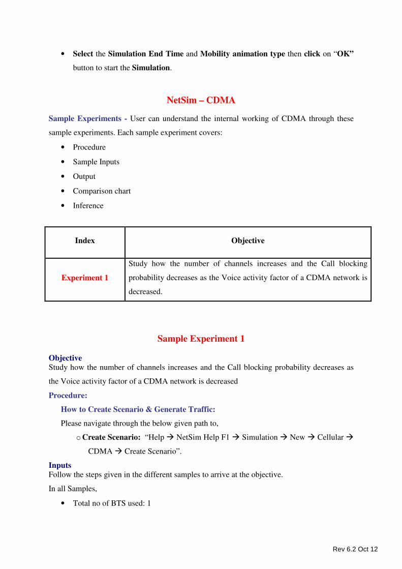
• Total no of MS used: 22
The devices are inter connected as given below,
• All the MS is placed in the range of BTS1
Set the properties of BTS and MS by following the tables for each sample,
MS Properties MS 1 MS 3 MS 5 MS 7 MS 9
Destination MS 2 MS 4 MS 6 MS 8 MS 10
Transmission
Type
Point to Point Point to
Point
Point to
Point
Point to
Point
Point to
Point
Traffic Type Voice Voice Voice Voice Voice
``Call Details
Distribution Exponential Exponential Exponential Exponential Exponential
Mean Call
Interval Time
(sec)
300 300 300 300 300
Distribution Exponential Exponential Exponential Exponential Exponential
Call Duration 60 60 60 60 60
Codec
Codec GSM-FR GSM-FR GSM-FR GSM-FR GSM-FR
Packet Size 33 33 33 33 33
Inter Arrival
Time (micro
sec)
20000 20000 20000 20000 20000
Service Type CBR CBR CBR CBR CBR
Generation rate 0.0132 0.0132 0.0132 0.0132 0.0132
Mobility
Model
No Mobility No Mobility No Mobility No Mobility No Mobility
Rev 6.2 Oct 12
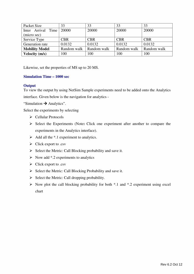
Likewise, MS 11 to MS 12, MS 13 to MS 14, MS 15 to MS 17 and MS 19 to MS 20.
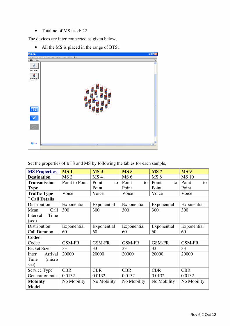
Inputs for Sample 1
BTS Properties BTS
Standards IS95A/B
Total bandwidth 1.25 MHz
Chip rate 1.2288 McPS
Voice Activity factor 1.0
Transmitter power 20 W
Path loss exponent 3
Fading figure 0.5
Standard deviation 11
Change the voice activity factor from 1.0, 0.9, 0.8, 0.7…. to 0.1.
Simulation Time – 1000 sec
Output To view the output by using NetSim Sample experiments need to be added onto the Analytics
interface. Given below is the navigation for analytics -
“Simulation ���� Analytics”.
Select the experiments by selecting
� Cellular Protocols
� Select the Experiments (Note: Click one experiment after another to compare the
experiments in the Analytics interface).
� Select the Metric: Call Blocking probability & Number of channel
Rev 6.2 Oct 12
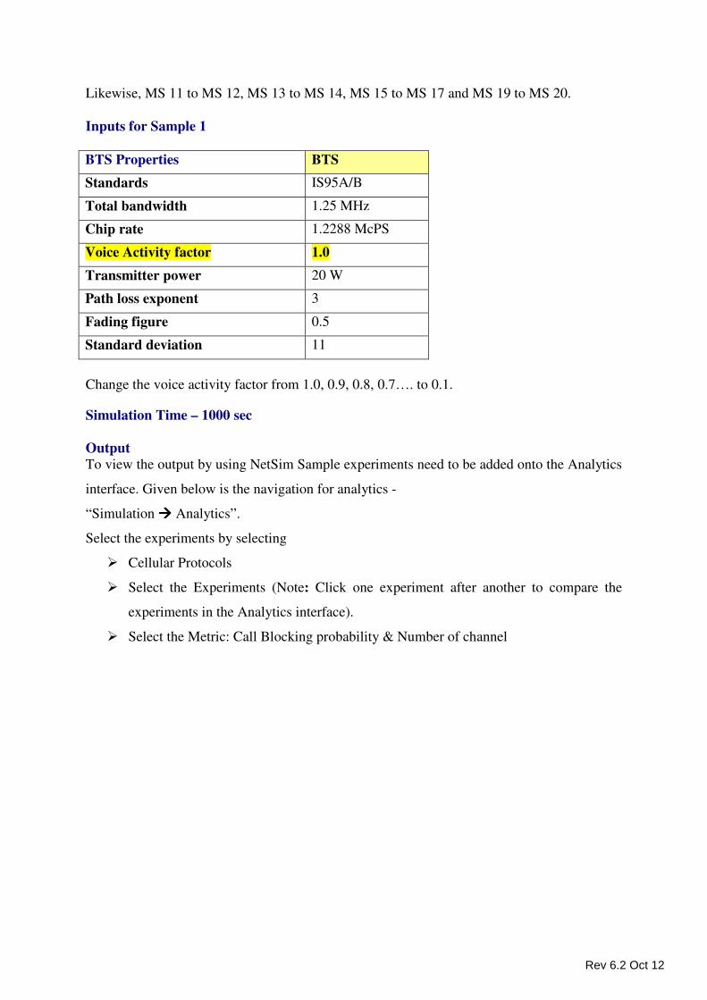
Comparison Charts and Inference:
Chart 1
When the system Voice activity factor decreases from 1.0 to 0.1, the number of channels
increases from 3 to 37. (Note: All other parameters like Bandwidth 1.25 MHz, chip rate
1.2288McPS, target SNR 6, Path loss exponent 3, Fading figure 0, and standard deviation 11,
are constant in all the samples taken.)
In CDMA network, the number of channels is inversely proportional to the voice activity
factor.
Chart 1 is a mirrored form of the x
y1
= graph. (This is because VAF is decreasing along +
ve X)
Voice activity factor
1
Number of
channels
α
Rev 6.2 Oct 12
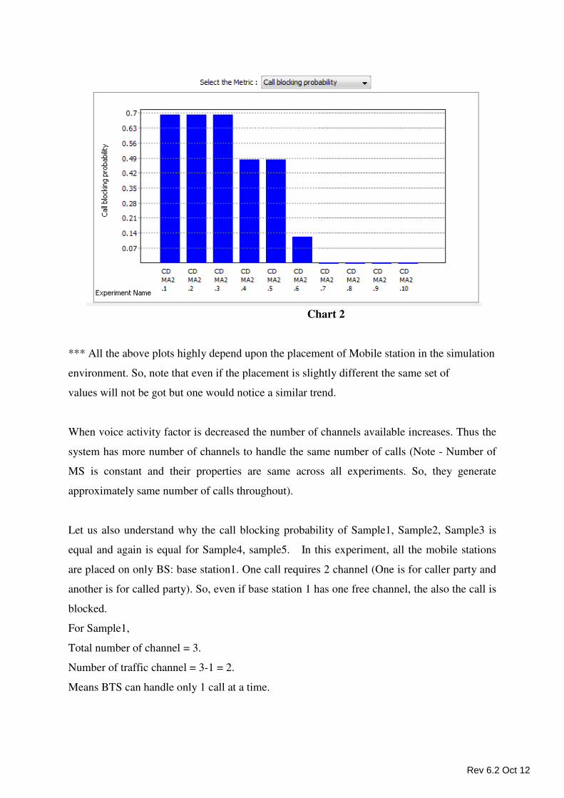
Chart 2
*** All the above plots highly depend upon the placement of Mobile station in the simulation
environment. So, note that even if the placement is slightly different the same set of
values will not be got but one would notice a similar trend.
When voice activity factor is decreased the number of channels available increases. Thus the
system has more number of channels to handle the same number of calls (Note - Number of
MS is constant and their properties are same across all experiments. So, they generate
approximately same number of calls throughout).
Let us also understand why the call blocking probability of Sample1, Sample2, Sample3 is
equal and again is equal for Sample4, sample5. In this experiment, all the mobile stations
are placed on only BS: base station1. One call requires 2 channel (One is for caller party and
another is for called party). So, even if base station 1 has one free channel, the also the call is
blocked.
For Sample1,
Total number of channel = 3.
Number of traffic channel = 3-1 = 2.
Means BTS can handle only 1 call at a time.
Rev 6.2 Oct 12
For Sample2,
Total number of channel = 4
Number of traffic channel = 4-1 = 3.
So, here also in this particular scenario where caller and called party are in BTS1, BTS1 can
handle only 1 call at a time. The 1 extra channel that is not available in sample1 is wasted
throughout. So, number of blocked calls or call blocking probability is same as sample1.
Global System for Mobile Communication (GSM)
New Experiments
In the Simulation menu select � New � Cellular � GSM
To perform experiments in GSM, the following steps should be followed,
• Create Scenario
• Set Mobile Station Properties
• Set Base Station (BS) Properties
• Remove Devices
• Simulate
Create Scenario
Adding Base Station - Click on the Base Station icon and drag it onto the environment
builder.
Adding Mobile Station -
• Click on the Mobile Station icon, drag, and drop it on the Base Station coverage
area.
• Mobile Station cannot be placed on another Mobile Station. It has to be dragged
and placed on the Base Station coverage area.
Remove Devices
Remove Mobile Station - Right click on the appropriate Mobile Station and click
Remove.
Remove Base Station - Right click on the appropriate Base Station and click Remove.
Note:
• If a Mobile Station which has already traffic is removed, all traffic originating
from this Mobile Station is also be deleted.
Rev 6.2 Oct 12
• In cases where the Base Station is in a network, firstly all Mobile Station needs to
be removed. Subsequently the Base Station can be removed. Base station can only
be removed in order.
Set Base Station (BS) Properties Right click on the appropriate Base Station (BS) and click Properties. Options available
are,
Wireless Properties - Under Wireless Properties tab the options available are,
• Device Type – This property defines the current device type. Base Station is set as
default.
• Connected To - This property defines the Wireless medium connected to the Base
Station (BS). A default value is already entered; hence no changes can be done.
• Global System for Mobile Communication
• Up Link Bandwidth – This property defines the range of uplink bandwidth that is
going too used for transmission. By default, 915 and 890 is set as Max and Min.
• Down Link Bandwidth – This property defines the range of downlink bandwidth that
is going too used for transmission. By default, 960 and 935 is set as Max and Min.
This value if auto set based on the value entered in the uplink bandwidth.
• Handover type - This property specifies that the hard handover be use as a
Handover technique.
• Channel Bandwidth – This property defines the channel bandwidth of one channel
used by GSM system. The value is fixed at 200 kHz.
• BTS Range – This property defines the range of BTS in km. The default value is set
as 1 km.
• Transmission Power (in W) – This property defines the transmission power used by
the current base station. 20W is set as default.
• Modulation Technique – This property define the modulation technique used by the
BTS. This value is fixed at GMSK.
• Channel Data Rate – This property defines the channel data rate used by GSM
system. This value is fixed at 270.83kbps.
• Multiple Access Technology – This property defines the multiple access technology
used by the GSM system. This is fixed as Time Division Multiple Access (TDMA).
• Speech Coding – This property denotes the speech coding technique used in the Base
station. This property is fixed at Linear Predictive Coding (LPC).
Rev 6.2 Oct 12
• Duplex Distance - This property denotes the duplex technique is used by the GSM
system. This property is fixed as Frequency Division Duplexing (FDD).
• Duplex Distance – This property denotes the duplex distance of GSM system. The
default value is 45 MHz.
• Number of slot in each carrier – This value denotes the number of slot in each
frequency carrier. The value is 8
Set Mobile Station Properties
Right Click on the appropriate Mobile Station to select Properties. Inside the properties
window click on Application1 to modify its properties.
Transmission Type
This indicates the type of transmission made by this Mobile station, Point to Point.
Destination
This property indicates the Destination Mobile Station.
Traffic Type
This property indicates the type of traffic. The traffic can only be Voice.
Voice
Call Details
Call Interval Time (Secs)
This property denotes the Call Interval Time. Each Call begins exponentially with mean
call inter arrival time. 300 sec is set as default Call Inter Arrival Time. User can select
450 secs or 600 secs as Call Interval Time.
Call Duration (Secs)
This property denotes how long the call continues. By default 60 secs is set as Call
duration.
User can select 120 and 240 secs as their call duration value.
Codec
Codec is the component of any voice system that translates between analog speech and the
bits used to transmit them. Every codec transmits a burst of data in a packet that can be
reconstructed into voice.
Service Type
• CBR - CBR stands for Constant Bit Rate. Packets of constant size are generated
at constant inter arrival times.
Click OK to accept the user entered values. Click on the close button at the top
right corner to exit the screen.
Rev 6.2 Oct 12
Packet Size
Packet Size (Bytes): Based on Codec Selection Packet Size can be set.
Inter Arrival Time
This indicates the time gap between packets. Based on Codec selection Inter Arrival
Time can be set.
Generation Rate
This denotes the Traffic Generation rate by the Mobile Station. Based on Packet size
and Inter Arrival Time Generation Rate can be set.
Click OK to accept the user entered values. Click on the close button at the top right
Corner to exit the screen.
Mobility Management Layer
Mobility Model
This property denotes which mobility model is used for performing the mobility. By
Default, No Mobility is used. Another available option is Random Walk Model.
Velocity (m/s)
This property denotes velocity of the mobile station if and only is Random Walk Model
is selected. By default 20 is set as default velocity.
Global System for Mobile Station (GSM) Properties:
Data Link Layer
Protocol
This property denotes Protocol used in the Data Link Layer. GSM is set as default
protocol.
Mobile Number
This property denotes the mobile number of the Mobile station.
IMEI No.
This property denotes the IMEI number of the Mobile station.
Rev 6.2 Oct 12

Physical Layer
Modulation Technique
This property denotes the type of modulation technique used in the Mobile Station.
GMSK is
set as default.
Transmission Power
This property denotes the transmission power of the mobile station.
Click Accept button.
Modifying/Viewing/Accepting Properties
On opening an already configured properties of an application the input fields will be
frozen
(i.e. the input cannot be changed).To modify these values click on the Modify button in
the screen. Now the input value can be changed. Click on the Accept button, the
modified values will be saved.
This View button is enabled once the Accept Button is clicked. To view the given values,
click on the View button.
Simulate - After creating the Scenario the following steps need to be followed,
• Click on Validate button.
• Click on Simulate button.
• Select the Simulation End Time and Mobility animation type then click on “OK”
button to start the Simulation.
NetSim – GSM
Sample Experiments - User can understand the internal working of GSM through these
sample experiments. Each sample experiment covers:
• Procedure
• Sample Inputs
• Output
• Comparison chart
Rev 6.2 Oct 12
• Inference
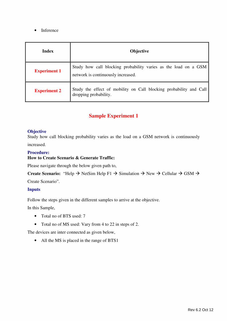
Index Objective
Experiment 1 Study how call blocking probability varies as the load on a GSM
network is continuously increased.
Experiment 2 Study the effect of mobility on Call blocking probability and Call
dropping probability.
Sample Experiment 1
Objective Study how call blocking probability varies as the load on a GSM network is continuously
increased.
Procedure:
How to Create Scenario & Generate Traffic:
Please navigate through the below given path to,
Create Scenario: “Help � NetSim Help F1 � Simulation � New � Cellular � GSM �
Create Scenario”.
Inputs
Follow the steps given in the different samples to arrive at the objective.
In this Sample,
• Total no of BTS used: 7
• Total no of MS used: Vary from 4 to 22 in steps of 2.
The devices are inter connected as given below,
• All the MS is placed in the range of BTS1
Rev 6.2 Oct 12
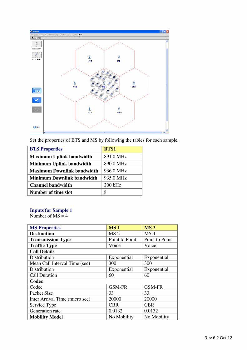
Set the properties of BTS and MS by following the tables for each sample,
BTS Properties BTS1
Maximum Uplink bandwidth 891.0 MHz
Minimum Uplink bandwidth 890.0 MHz
Maximum Downlink bandwidth 936.0 MHz
Minimum Downlink bandwidth 935.0 MHz
Channel bandwidth 200 kHz
Number of time slot 8
Inputs for Sample 1 Number of MS = 4
MS Properties MS 1 MS 3
Destination MS 2 MS 4
Transmission Type Point to Point Point to Point
Traffic Type Voice Voice
Call Details
Distribution Exponential Exponential
Mean Call Interval Time (sec) 300 300
Distribution Exponential Exponential
Call Duration 60 60
Codec
Codec GSM-FR GSM-FR
Packet Size 33 33
Inter Arrival Time (micro sec) 20000 20000
Service Type CBR CBR
Generation rate 0.0132 0.0132
Mobility Model No Mobility No Mobility
Rev 6.2 Oct 12
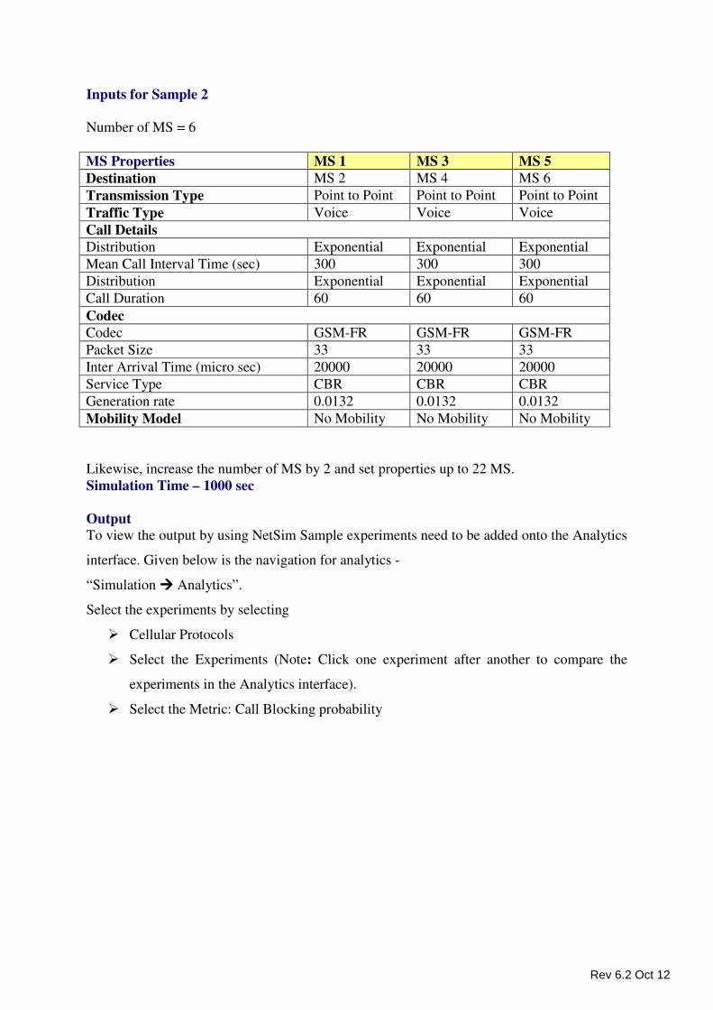
Inputs for Sample 2
Number of MS = 6
MS Properties MS 1 MS 3 MS 5
Destination MS 2 MS 4 MS 6
Transmission Type Point to Point Point to Point Point to Point
Traffic Type Voice Voice Voice
Call Details
Distribution Exponential Exponential Exponential
Mean Call Interval Time (sec) 300 300 300
Distribution Exponential Exponential Exponential
Call Duration 60 60 60
Codec
Codec GSM-FR GSM-FR GSM-FR
Packet Size 33 33 33
Inter Arrival Time (micro sec) 20000 20000 20000
Service Type CBR CBR CBR
Generation rate 0.0132 0.0132 0.0132
Mobility Model No Mobility No Mobility No Mobility
Likewise, increase the number of MS by 2 and set properties up to 22 MS.
Simulation Time – 1000 sec
Output To view the output by using NetSim Sample experiments need to be added onto the Analytics
interface. Given below is the navigation for analytics -
“Simulation ���� Analytics”.
Select the experiments by selecting
� Cellular Protocols
� Select the Experiments (Note: Click one experiment after another to compare the
experiments in the Analytics interface).
� Select the Metric: Call Blocking probability
Rev 6.2 Oct 12
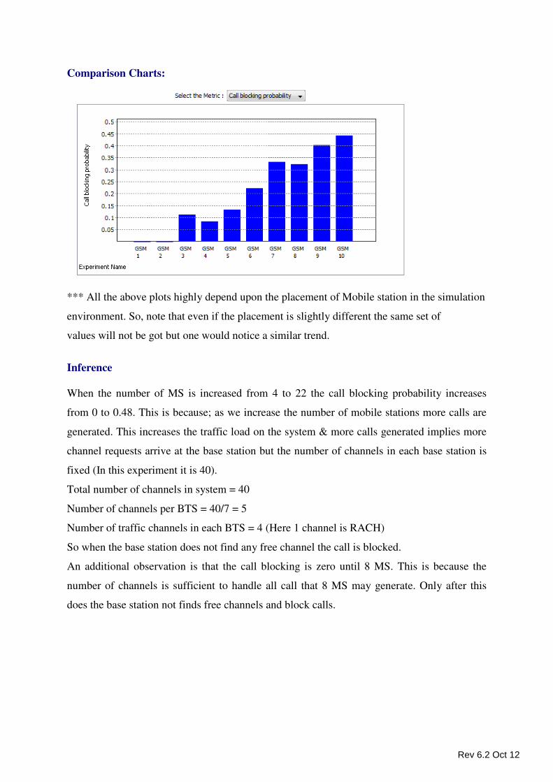
Comparison Charts:
*** All the above plots highly depend upon the placement of Mobile station in the simulation
environment. So, note that even if the placement is slightly different the same set of
values will not be got but one would notice a similar trend.
Inference
When the number of MS is increased from 4 to 22 the call blocking probability increases
from 0 to 0.48. This is because; as we increase the number of mobile stations more calls are
generated. This increases the traffic load on the system & more calls generated implies more
channel requests arrive at the base station but the number of channels in each base station is
fixed (In this experiment it is 40).
Total number of channels in system = 40
Number of channels per BTS = 40/7 = 5
Number of traffic channels in each BTS = 4 (Here 1 channel is RACH)
So when the base station does not find any free channel the call is blocked.
An additional observation is that the call blocking is zero until 8 MS. This is because the
number of channels is sufficient to handle all call that 8 MS may generate. Only after this
does the base station not finds free channels and block calls.
Rev 6.2 Oct 12
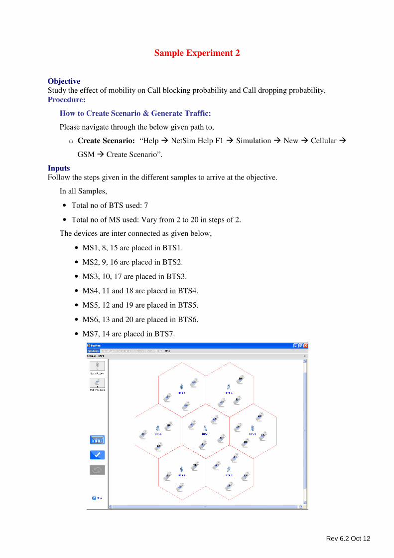
Sample Experiment 2
Objective Study the effect of mobility on Call blocking probability and Call dropping probability.
Procedure:
How to Create Scenario & Generate Traffic:
Please navigate through the below given path to,
o Create Scenario: “Help � NetSim Help F1 � Simulation � New � Cellular �
GSM � Create Scenario”.
Inputs Follow the steps given in the different samples to arrive at the objective.
In all Samples,
• Total no of BTS used: 7
• Total no of MS used: Vary from 2 to 20 in steps of 2.
The devices are inter connected as given below,
• MS1, 8, 15 are placed in BTS1.
• MS2, 9, 16 are placed in BTS2.
• MS3, 10, 17 are placed in BTS3.
• MS4, 11 and 18 are placed in BTS4.
• MS5, 12 and 19 are placed in BTS5.
• MS6, 13 and 20 are placed in BTS6.
• MS7, 14 are placed in BTS7.
Rev 6.2 Oct 12
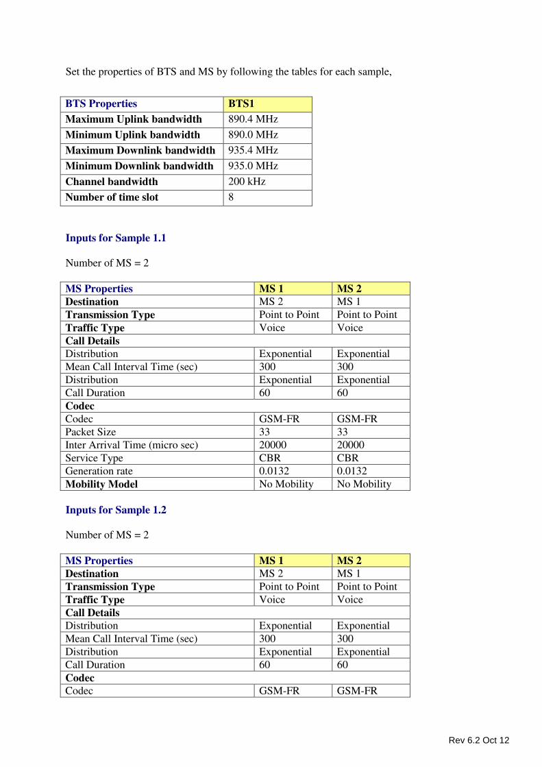
Set the properties of BTS and MS by following the tables for each sample,
BTS Properties BTS1
Maximum Uplink bandwidth 890.4 MHz
Minimum Uplink bandwidth 890.0 MHz
Maximum Downlink bandwidth 935.4 MHz
Minimum Downlink bandwidth 935.0 MHz
Channel bandwidth 200 kHz
Number of time slot 8
Inputs for Sample 1.1
Number of MS = 2
MS Properties MS 1 MS 2
Destination MS 2 MS 1
Transmission Type Point to Point Point to Point
Traffic Type Voice Voice
Call Details
Distribution Exponential Exponential
Mean Call Interval Time (sec) 300 300
Distribution Exponential Exponential
Call Duration 60 60
Codec
Codec GSM-FR GSM-FR
Packet Size 33 33
Inter Arrival Time (micro sec) 20000 20000
Service Type CBR CBR
Generation rate 0.0132 0.0132
Mobility Model No Mobility No Mobility
Inputs for Sample 1.2
Number of MS = 2
MS Properties MS 1 MS 2
Destination MS 2 MS 1
Transmission Type Point to Point Point to Point
Traffic Type Voice Voice
Call Details
Distribution Exponential Exponential
Mean Call Interval Time (sec) 300 300
Distribution Exponential Exponential
Call Duration 60 60
Codec
Codec GSM-FR GSM-FR
Rev 6.2 Oct 12
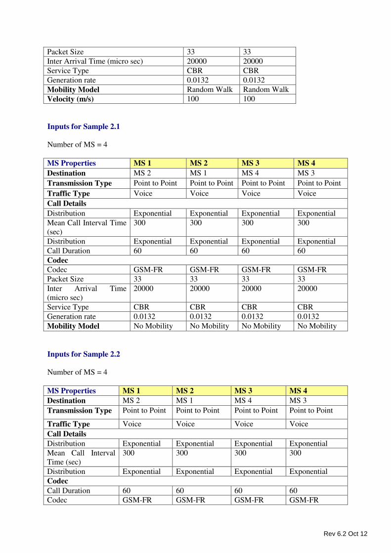
Packet Size 33 33
Inter Arrival Time (micro sec) 20000 20000
Service Type CBR CBR
Generation rate 0.0132 0.0132
Mobility Model Random Walk Random Walk
Velocity (m/s) 100 100
Inputs for Sample 2.1
Number of MS = 4
MS Properties MS 1 MS 2 MS 3 MS 4
Destination MS 2 MS 1 MS 4 MS 3
Transmission Type Point to Point Point to Point Point to Point Point to Point
Traffic Type Voice Voice Voice Voice
Call Details
Distribution Exponential Exponential Exponential Exponential
Mean Call Interval Time
(sec)
300 300 300 300
Distribution Exponential Exponential Exponential Exponential
Call Duration 60 60 60 60
Codec
Codec GSM-FR GSM-FR GSM-FR GSM-FR
Packet Size 33 33 33 33
Inter Arrival Time
(micro sec)
20000 20000 20000 20000
Service Type CBR CBR CBR CBR
Generation rate 0.0132 0.0132 0.0132 0.0132
Mobility Model No Mobility No Mobility No Mobility No Mobility
Inputs for Sample 2.2
Number of MS = 4
MS Properties MS 1 MS 2 MS 3 MS 4
Destination MS 2 MS 1 MS 4 MS 3
Transmission Type Point to Point Point to Point Point to Point Point to Point
Traffic Type Voice Voice Voice Voice
Call Details
Distribution Exponential Exponential Exponential Exponential
Mean Call Interval
Time (sec)
300 300 300 300
Distribution Exponential Exponential Exponential Exponential
Codec
Call Duration 60 60 60 60
Codec GSM-FR GSM-FR GSM-FR GSM-FR
Rev 6.2 Oct 12
Packet Size 33 33 33 33
Inter Arrival Time
(micro sec)
20000 20000 20000 20000
Service Type CBR CBR CBR CBR
Generation rate 0.0132 0.0132 0.0132 0.0132
Mobility Model Random walk Random walk Random walk Random walk
Velocity (m/s) 100 100 100 100
Likewise, set the properties of MS up to 20 MS.
Simulation Time – 1000 sec
Output To view the output by using NetSim Sample experiments need to be added onto the Analytics
interface. Given below is the navigation for analytics -
“Simulation ���� Analytics”.
Select the experiments by selecting
� Cellular Protocols
� Select the Experiments (Note: Click one experiment after another to compare the
experiments in the Analytics interface).
� Add all the *.1 experiment to analytics.
� Click export to .csv
� Select the Metric: Call Blocking probability and save it.
� Now add *.2 experiments to analytics
� Click export to .csv
� Select the Metric: Call Blocking Probability and save it.
� Select the Metric: Call dropping probability.
� Now plot the call blocking probability for both *.1 and *.2 experiment using excel
chart
Rev 6.2 Oct 12
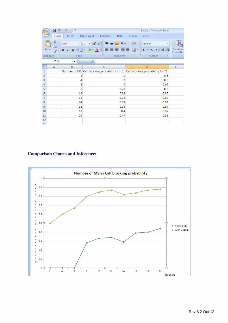
Comparison Charts and Inference:
Rev 6.2 Oct 12
*** All the above plots highly depend upon the placement of MS in the simulation
workspace. So, note that even if the placement is slightly different the same set of values will
not be got but one would notice a similar trend.
The call blocking probability is less in case of no mobility when compare to the same
scenario with mobility. This is because,
Total number of channel = 16.
Number of BTS = 7
So, Number of channel per BTS = 16/7 = 2.
Number of traffic channels = 2-1 = 1. Here 1 channel is the Random access channel.
From above calculation, it is clear that each base station can handle 1 call at a time.
Now, due to mobility it is likely that mobile station moves from one base station to another
and requests for handover. The new base station checks for free channels and if there is no
free channel available then that handover request fails and the call is dropped (As we see in
Chart 3). So, in case of mobility the network encounters extra blocking due to handover
failures. Hence, the call blocking probability is greater in case of mobility as compared to no
mobility. The call dropping probability also increases when number of MS increases as
explained in another GSM experiment.
If number of MS is, continuously increased then these two graphs will converge. For heavy
load, the call blocking probability due to new call request is much higher compared to
handover requests. So, the effect of handover on call blocking probability will be very small
and two graphs converge.
Pure Aloha
New Experiments
In the Simulation menu select � New � LAN � Aloha ���� Pure Aloha.
To perform experiments in Pure Aloha, the following steps should be followed,
• Create Scenario
• Set Node Properties
• Remove Devices
• Simulate
Rev 6.2 Oct 12
Create Scenario
Adding Node –
• Click on the Node icon and drag and drop it in side the Red Circle (i.e. Visibility
Range - The systems in this range can communicate among themselves only).
• Nodes are directly connected to each other as soon as they are dropped in this
range.
A Node cannot be placed on another Node. A Node cannot float outside the Red
Circle. It has to be dragged and placed inside the Visibility Range.
Set Node Properties
Right Click on the appropriate node to select Properties. Inside the properties’ window click
on Application 1 to modify its properties.
Transmission Type
This indicates the type of transmission made by this session, either Broadcast or Point to
Point.
Destination
This property indicates the Destination Node.
Traffic Type
This property indicates the type of traffic. The traffic can either be Voice or Data.
Voice
Codec
Codec is the component of any voice system that translates between analog speech and
the bits used to transmit them. Every codec transmits a burst of data in a packet that can
be reconstructed into voice. Five different standards of voice codec’s are given which can
be selected depending on the variations required.
Service Type
• CBR - CBR stands for Constant Bit Rate. Packets of constant size are generated at
constant inter arrival times.
• VBR - VBR stands for Variable Bit Rate. The two types of Suppression Model that
can be selected are,
• Deterministic
• Markov Chain
Click OK to accept the user entered values. Click on the close button at the top
right corner to exit the screen.
Rev 6.2 Oct 12
Data
Packet Size
Distribution: The options available for distribution are,
• Constant
• Exponential
Mean Packet Size (Bytes): Sets the size of the packets being generated by the chosen
distribution. The ranges of values that can be entered are between 65 to 1500 bytes.
By default 1500 bytes is entered.
Inter Arrival Time
This indicates the time gap between packets.
Distribution : The options available for distribution are,
• Constant
• Exponential
• Uniform
Mean Inter Arrival Time: Enter the average inter-arrival time between packets. A
lower inter-arrival time would lead to a higher generation rate and the vice versa. The
range of values that can be entered are between 1000 to 20000 Micro Sec. By default
20000 Micro Sec is entered.
Click OK to accept the user entered values. Click on the close button at the top right
corner to exit the screen.
Modifying/Viewing/Accepting Properties
On opening an already configured properties of an application the input fields will be
frozen (i.e. the input cannot be changed).To modify these values click on the Modify
button in the screen. Now the input value can be changed. Click on the Accept button,
the modified values will be saved.
This View button is enabled once the Accept Button is clicked. To view the given
values, click on the View button.
Remove Devices
Remove Node - Right click on the appropriate Node and click Remove.
Note -
• If a Node transmitting data is removed, all traffic originating from this Node is also
deleted.
Simulate - After creating the Scenario the following steps need to be followed,
• Click on Validate button.
• Click on Simulate button.
Rev 6.2 Oct 12
• Select the Simulation End Time and then Click on “OK” button to start the
Simulation.
Slotted Aloha
New Experiments
In the Simulation menu select � New � LAN � Aloha � Slotted Aloha
To perform experiments in Slotted Aloha, the following steps should be followed,
• Create Scenario
• Set Node Properties
• Remove Devices
• Simulate
Create Scenario
Adding Node -
• Click on the Node icon and drag and drop it in side the Red Circle (i.e. Visibility
Range - The systems in this range can communicate among themselves only).
• Nodes are directly connected to each other as soon as they are dropped in this
range.
A Node cannot be placed on another Node. A Node cannot float outside the Red
Circle. It has to be dragged and placed inside the Visibility Range.
Set Node Properties
Right Click on the appropriate node to select Properties. Inside the properties’ window click
on Application 1 to modify its properties.
Transmission Type
This indicates the type of transmission made by this session, either Broadcast or Point to
Point.
Destination
This property indicates the Destination Node.
Traffic Type
This property indicates the type of traffic. The traffic can either be Voice or Data.
Voice
Codec
Codec is the component of any voice system that translates between analog speech and
the bits used to transmit them. Every codec transmits a burst of data in a packet that can
Rev 6.2 Oct 12
be reconstructed into voice. Five different standards of voice codec’s are given which can
be selected depending on the variations required.
Service Type
• CBR - CBR stands for Constant Bit Rate. Packets of constant size are generated at
constant inter arrival times.
• VBR - VBR stands for Variable Bit Rate. The two types of Suppression Model that
can be selected are,
• Deterministic
• Markov Chain
Click OK to accept the user entered values. Click on the close button at the top
right corner to exit the screen.
Data
Packet Size
Distribution: The options available for distribution are,
• Constant
• Exponential
Mean Packet Size (Bytes): Sets the size of the packets being generated by the
chosen distribution. The range of values that can be entered are between 65 to 1500
bytes. By default 1500 bytes is entered.
Inter Arrival Time
This indicates the time gap between packets.
Distribution : The options available for distribution are,
• Constant
• Exponential
• Uniform
Mean Inter Arrival Time: Enter the average inter-arrival time between packets. A
lower inter-arrival time would lead to a higher generation rate and the vice versa.
The range of values that can be entered are between 1000 to 20000 Micro Sec. By
default 20000 Micro Sec is entered.
Click OK to accept the user entered values. Click on the close button at the top right
corner to exit the screen.
Modifying/Viewing/Accepting Properties
On opening an already configured properties of an application the input fields will be
frozen (i.e. the input cannot be changed).To modify these values click on the Modify
Rev 6.2 Oct 12
button in the screen. Now the input value can be changed. Click on the Accept button,
the modified values will be saved.
This View button is enabled once the Accept Button is clicked. To view the given
values, click on the View button.
Remove Devices
Remove Node - Right click on the appropriate Node and click Remove.
Note -
• If a Node transmitting data is removed, all traffic originating from this Node is also
deleted.
Simulate - After creating the Scenario the following steps need to be followed,
• Click on Validate button.
• Click on Simulate button.
• Select the Simulation End Time and then Click on “OK” button to start the
Simulation.
NetSim – Slotted Aloha
Sample Experiments - User can understand the internal working of Slotted Aloha through
these sample experiments. Each sample experiment covers:
• Procedure
• Sample Inputs
• Output
• Comparison chart
• Inference
Index Objective
Experiment 1 Study the throughput characteristics of a slotted aloha network
Rev 6.2 Oct 12
Sample Experiment 1
Objective: Plot the characteristic curve throughput versus offered traffic for a Slotted
ALOHA system.
(Reference: Computer Networks, 3rd Edition. Andrew S. Tanenbaum)
Theory:
ALOHA provides a wireless data network. It is a multiple access protocol (this protocol is for
allocating a multiple access channel). There are two main versions of ALOHA: pure and
slotted. They differ with respect to whether or not time is divided up into discrete slots into
which all frames must fit.
Slotted ALOHA:
In slotted Aloha, time is divided up into discrete intervals, each interval corresponding to one
frame. In Slotted ALOHA, a computer is required to wait for the beginning of the next slot in
order to send the next packet. The probability of no other traffic being initiated during the
entire vulnerable period is given by which leads to
Where, S (frames per frame time) is the mean of the Poisson distribution with which frames
are being generated. For reasonable throughput S should lie between 0 and 1.
G is the mean of the Poisson distribution followed by the transmission attempts per frame
time, old and new combined. Old frames mean those frames that have previously suffered
collisions.
It is easy to note that Slotted ALOHA peaks at G=1, with a throughput of or about
0.368. It means that if the system is operating at G=1, the probability of an empty an slot is
0.368
Calculations used in NetSim to obtain the plot between S and G:
Using NetSim, the attempts per packet time (G) can be calculated as follows;
G= TA*PT/(ST*1000)
Where, G= attempts per packet time
TA=Total Attempt
PT= Packet time (in milli seconds)
ST=Simulation time (in seconds)
The throughput (mbps) per frame time can be obtained as follows:
Rev 6.2 Oct 12
S=Throughput (in Mbps)*1000*PT/PS*8
Where, S= Throughput per frame time
PT=Packet time (in milli seconds)
PS=Packet size (in bytes)
Calculations for the packet time:
PT= packet size (bits)/ Bandwidth (Mbps)
In the following experiment we have taken packet size=1498 bytes (1472 + 26 Overheads)
Bandwidth is 10 Mbps and hence, packet time comes as 1.198 ms.
Procedure:
How to Create Scenario:
Create Scenario: “Help � Simulation � New � LAN � Aloha�Slotted
Aloha�Create Scenario”.
Obtain the values of Throughput and Total Attempts from the statistics of NetSim simulation
for various numbers of traffic generators.
Sample Inputs:
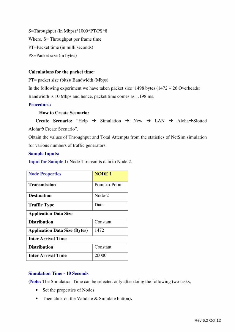
Input for Sample 1: Node 1 transmits data to Node 2.
Simulation Time - 10 Seconds
(Note: The Simulation Time can be selected only after doing the following two tasks,
• Set the properties of Nodes
• Then click on the Validate & Simulate button).
Node Properties NODE 1
Transmission Point-to-Point
Destination Node-2
Traffic Type Data
Application Data Size
Distribution Constant
Application Data Size (Bytes) 1472
Inter Arrival Time
Distribution Constant
Inter Arrival Time 20000
Rev 6.2 Oct 12
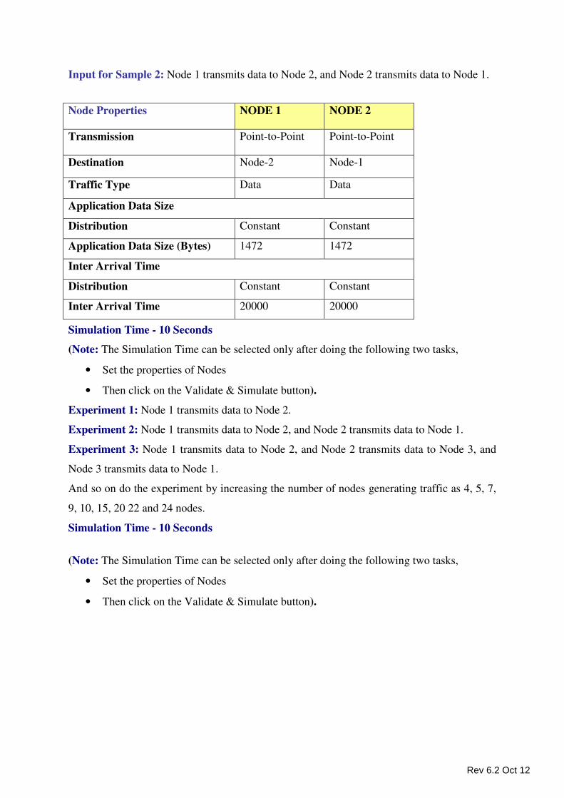
Input for Sample 2: Node 1 transmits data to Node 2, and Node 2 transmits data to Node 1.
Simulation Time - 10 Seconds
(Note: The Simulation Time can be selected only after doing the following two tasks,
• Set the properties of Nodes
• Then click on the Validate & Simulate button).
Experiment 1: Node 1 transmits data to Node 2.
Experiment 2: Node 1 transmits data to Node 2, and Node 2 transmits data to Node 1.
Experiment 3: Node 1 transmits data to Node 2, and Node 2 transmits data to Node 3, and
Node 3 transmits data to Node 1.
And so on do the experiment by increasing the number of nodes generating traffic as 4, 5, 7,
9, 10, 15, 20 22 and 24 nodes.
Simulation Time - 10 Seconds
(Note: The Simulation Time can be selected only after doing the following two tasks,
• Set the properties of Nodes
• Then click on the Validate & Simulate button).
Node Properties NODE 1 NODE 2
Transmission Point-to-Point Point-to-Point
Destination Node-2 Node-1
Traffic Type Data Data
Application Data Size
Distribution Constant Constant
Application Data Size (Bytes) 1472 1472
Inter Arrival Time
Distribution Constant Constant
Inter Arrival Time 20000 20000
Rev 6.2 Oct 12
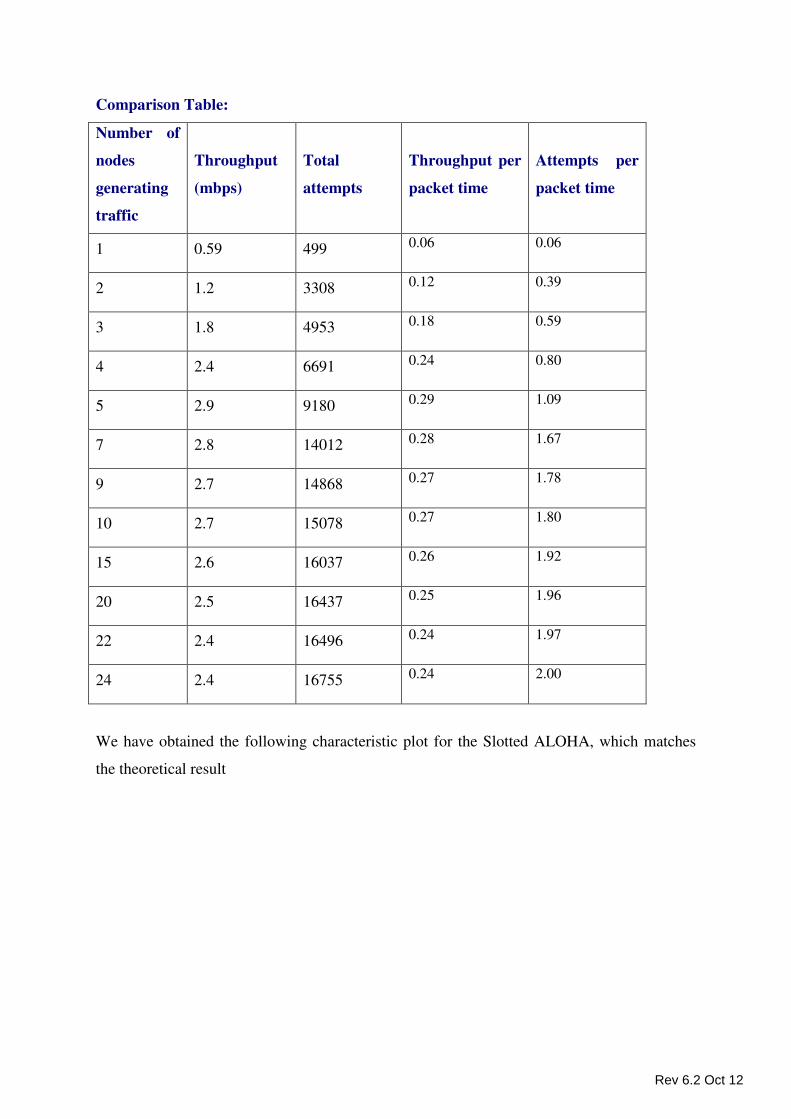
Comparison Table:
Number of
nodes
generating
traffic
Throughput
(mbps)
Total
attempts
Throughput per
packet time
Attempts per
packet time
1 0.59 499 0.06 0.06
2 1.2 3308 0.12 0.39
3 1.8 4953 0.18 0.59
4 2.4 6691 0.24 0.80
5 2.9 9180 0.29 1.09
7 2.8 14012 0.28 1.67
9 2.7 14868 0.27 1.78
10 2.7 15078 0.27 1.80
15 2.6 16037 0.26 1.92
20 2.5 16437 0.25 1.96
22 2.4 16496 0.24 1.97
24 2.4 16755 0.24 2.00
We have obtained the following characteristic plot for the Slotted ALOHA, which matches
the theoretical result
Rev 6.2 Oct 12
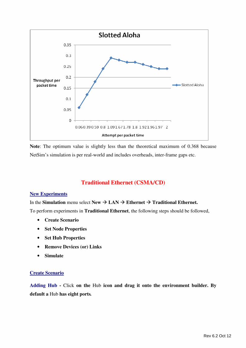
Note: The optimum value is slightly less than the theoretical maximum of 0.368 because
NetSim’s simulation is per real-world and includes overheads, inter-frame gaps etc.
Traditional Ethernet (CSMA/CD)
New Experiments
In the Simulation menu select New � LAN � Ethernet � Traditional Ethernet.
To perform experiments in Traditional Ethernet, the following steps should be followed,
• Create Scenario
• Set Node Properties
• Set Hub Properties
• Remove Devices (or) Links
• Simulate
Create Scenario
Adding Hub - Click on the Hub icon and drag it onto the environment builder. By
default a Hub has eight ports.
Rev 6.2 Oct 12
Adding Node –
• Click on the Node icon and drag and drop it on the Hub.
• Nodes cannot be connected directly to each other because an intermediate
connecting component (such as Hub) is required.
• A Node cannot be placed on another Node and it cannot float without a connection.
It has to be dragged and placed on any connecting component.
Establishing Connections between two Hubs - Click the two devices to connect them.
These two devices are connected via a Link.
Set Node Properties
Right Click on the appropriate Node to select Properties. Inside the properties’ window
clicks on Application1 to modify its properties.
Transmission Type
This indicates the type of transmission made by this session, either Broadcast or Point to
Point.
Destination
This property indicates the Destination Node.
Traffic Type
This property indicates the type of traffic. The traffic can either be Voice or Data.
Voice
Codec
Codec is the component of any voice system that translates between analog speech and
the bits used to transmit them. Every codec transmits a burst of data in a packet that can
be reconstructed into voice. Five different standards of voice codec’s are given which
can be selected depending on the variations required.
Service Type
• CBR - CBR stands for Constant Bit Rate. Packets of constant size are generated at
constant inter arrival times.
• VBR - VBR stands for Variable Bit Rate. The two types of Suppression Model
that can be selected are,
• Deterministic
• Markov Chain
Click OK to accept the user entered values. Click on the close button at the top
right corner to exit the screen.
Rev 6.2 Oct 12
Data
Packet Size
Distribution: The options available for distribution are,
• Constant
• Exponential
Mean Packet Size (Bytes): Sets the size of the packets being generated by the
chosen distribution. The range of values that can be entered are between 65 to 1500
bytes. By default 1500 bytes is entered.
Inter Arrival Time
This indicates the time gap between packets.
Distribution: The options available for distribution are,
• Constant
• Exponential
• Uniform
Mean Inter Arrival Time: Enter the average inter-arrival time between packets.
A lower inter-arrival time would lead to a higher generation rate and the vice versa.
The range of values that can be entered are between 1000 to 20000 Micro Sec. By
default 20000 Micro Sec is entered.
Click OK to accept the user entered values. Click on the close button at the top
right corner to exit the screen.
Persistence
Select the values from the dropdown menu. The value ranges from 1, ½, 1/3 ….to,
1/15. Default value available is 1.
Modifying/Viewing/Accepting Properties
On opening an already configured properties of an application the input fields will be
frozen (i.e. the input cannot be changed).To modify these values click on the Modify
button in the screen. Now the input value can be changed. Click on the Accept button,
the modified values will be saved.
This View button is enabled once the Accept Button is clicked. To view the given
values, click on the View button.
Set Hub Properties
Right click on the appropriate Hub and click Properties.
Device Id - This property is a value that is generated automatically. Each Id generated is
unique.
Port Properties - The Port Properties for each Port are as follows,
Data Rate (Mbps) - This defines the underlying data rate. Option available is 10
Mbps indicates 10 Mega Bits per Second (default value)
Error Rate (BER) - This defines the rate of the error. Options available are
Rev 6.2 Oct 12
• No Error indicates zero error during transmission (default value).
• 10^-6 indicates one error in every 1,000,000 bits transmitted.
• 10^-7 indicates one error in every 10,000,000 bits transmitted.
• 10^-8 indicates one error in every 100,000,000 bits transmitted.
• 10^-9 indicates one error in every 1000,000,000 bits transmitted.
Physical Medium - This defines the type of Physical Medium. Twisted Pair is the
only option available.
Persistence - Options available are ���� “1, 1/2, 1/3, 1/4… 1/15”. Default value is 1.
Connected To – This property gives the Node number to the Port number
selected.
Communication - This property defines the mode of Communication. By
default, a star topology network works in Half Duplex. This property cannot be
changed.
Remove Devices / Links
Remove Link - Right click on the appropriate Link and click Remove.
Remove Node - Right click on the appropriate Node and click Remove.
Remove Hub - Right click on the appropriate Hub and click Remove.
Note -
• If a Node transmitting data is removed, all traffic originating from this Node is also
deleted.
• In cases where the Hub is in a network (connected to other Hubs), firstly the
connection need to be removed. Subsequently the Hub can be removed
Simulate - After creating the Scenario the following steps need to be followed,
• Click on Validate button.
• Click on Simulate button.
• Select the Simulation End Time and then click on “OK” button to start the
Simulation.
NetSim - Traditional Ethernet
Sample Experiments - User can understand the internal working of Traditional Ethernet
through these sample experiments. Each sample experiment covers:
• Procedure
• Sample Inputs
Rev 6.2 Oct 12
• Output
• Comparison chart
• Inference
Index Objective
Experiment 1 Understand the impact of bit error rate on packet error rate and investigate
the impact of error of a simple hub based CSMA / CD network
Experiment 2 To determine the optimum persistence of a p-persistent CSMA / CD
network for a heavily loaded bus capacity.
Sample Experiment 1
Objective:
Understand the impact of Bit error rate on packet error rate and investigate the impact of error
of a simple hub based CSMA / CD network
Theory:
Bit error rate (BER): The bit error rate or bit error ratio is the number of bit errors divided
by the total number of transferred bits during a studied time interval i.e.
BER=Bit errors/Total number of bits
For example, a transmission might have a BER of 10-5
, meaning that on average, 1 out of
every of 100,000 bits transmitted exhibits an error. The BER is an indication of how often a
packet or other data unit has to be retransmitted because of an error.
Unlike many other forms of assessment, bit error rate, BER assesses the full end to end
performance of a system including the transmitter, receiver and the medium between the two.
In this way, bit error rate, BER enables the actual performance of a system in operation to be
tested.
Bit error probability (pe): The bit error probability is the expectation value of the BER. The
BER can be considered as an approximate estimate of the bit error probability. This estimate
is accurate for a long time interval and a high number of bit errors.
Rev 6.2 Oct 12
Packet Error Rate (PER):
The PER is the number of incorrectly received data packets divided by the total number of
received packets. A packet is declared incorrect if at least one bit is erroneous. The
expectation of the PER is denoted as packet error probability pp , which for a data packet
length of N bits can be expressed as
It is based on the assumption that the bit errors are independent of each other.
Derivation of the packet error probability:
Suppose packet size is N bits.
is the bit error probability then probability of no bit error=1-
As packet size is N bits and it is the assumption that the bit errors are independent. Hence,
Probability of a packet with no errors =
A packet is erroneous if at least there is one bit error, hence
Probability of packet error=1-
Procedure:
How to create a scenario and generate traffic:
Create Scenario: Help � Simulation � New � LAN � Ethernet� Traditional Ethernet
� Create Scenario.
Example 1:
Create samples by varying the bit error rate (10-6
, 10-7
, 10-8
, 10-9
, No error) and check
whether packet error output matches the PER formula.
Sample Inputs:
In this sample experiment, two nodes and one hub are dragged and dropped on the
environment builder. And following experiments are performed.
Inputs for the sample experiments are given below,
• Drag and drop Hub on the environment builder.
• Drag and drop Node1 over the hub.
• Drag and drop Node2 over the hub.
Node Properties Node1
Transmission Type Point to Point
Destination 2
Application Data Size (Bytes) 1472
Distribution Constant
Rev 6.2 Oct 12
Inter Arrival Time (µs) 2500
MTU Size(Bytes) 1500
Hub Properties Sample1 Sample 2 Sample 3 Sample 4 Sample 5
Data rate (Mbps) 10 10 10 10 10
Error Rate (BER) No Error 10-9
10-8
10-7
10-6
Physical Medium Twisted
Pair
Twisted
Pair
Twisted
Pair
Twisted
Pair
Twisted
Pair
Simulation Time - 1000 Sec
(Note: The Simulation Time can be selected only after the following two tasks,
• Set the properties for the Node1 & The Hub
• Click on the Validate & Simulate button).
NetSim simulation output:
BER Error
packets
Total
packets
PER(Error
packets/Total
packets)
PER-using the formula
Throughput
(mbps)
0 1E-
09 1E-
08 1E-
07 1E-
06
0
4
57
470
4730
400000
400000
400000
400000
400000
0
0.00001
0.0001425
0.001175
0.011825
0
0.000011999
0.000119993
0.00119928
0.011928293
4.71
4.71
4.71
4.7
4.65
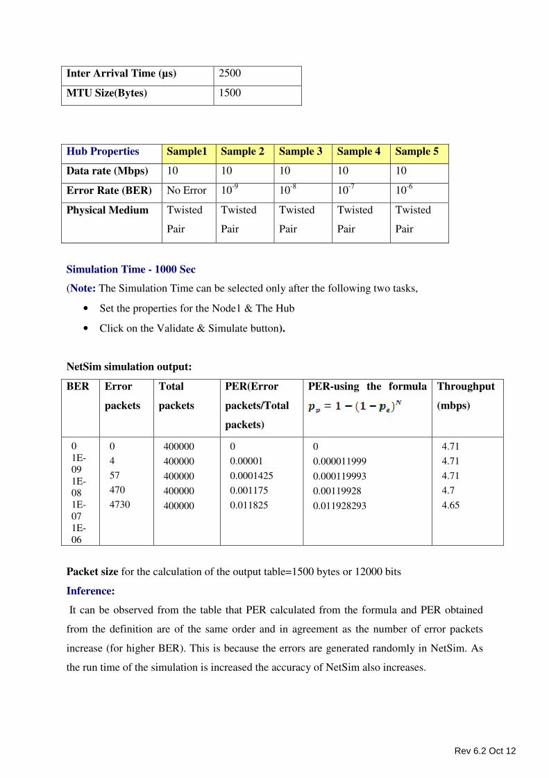
Packet size for the calculation of the output table=1500 bytes or 12000 bits
Inference:
It can be observed from the table that PER calculated from the formula and PER obtained
from the definition are of the same order and in agreement as the number of error packets
increase (for higher BER). This is because the errors are generated randomly in NetSim. As
the run time of the simulation is increased the accuracy of NetSim also increases.
Rev 6.2 Oct 12
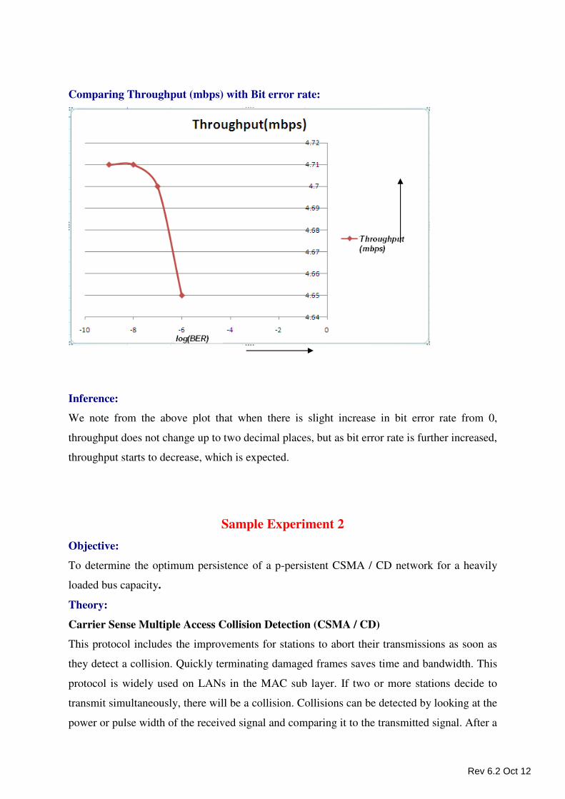
Comparing Throughput (mbps) with Bit error rate:
Inference:
We note from the above plot that when there is slight increase in bit error rate from 0,
throughput does not change up to two decimal places, but as bit error rate is further increased,
throughput starts to decrease, which is expected.
Sample Experiment 2
Objective:
To determine the optimum persistence of a p-persistent CSMA / CD network for a heavily
loaded bus capacity.
Theory:
Carrier Sense Multiple Access Collision Detection (CSMA / CD)
This protocol includes the improvements for stations to abort their transmissions as soon as
they detect a collision. Quickly terminating damaged frames saves time and bandwidth. This
protocol is widely used on LANs in the MAC sub layer. If two or more stations decide to
transmit simultaneously, there will be a collision. Collisions can be detected by looking at the
power or pulse width of the received signal and comparing it to the transmitted signal. After a
Rev 6.2 Oct 12
station detects a collision, it aborts its transmission, waits a random period of time and then
tries again, assuming that no other station has started transmitting in the meantime.
There are mainly three theoretical versions of the CSMA /CD protocol:
1-persistent CSMA / CD: When a station has data to send, it first listens to the channel to
see if anyone else is transmitting at that moment. If the channel is busy, the station waits until
it becomes idle. When station detects an idle channel, it transmits a frame. If a collision
occurs, the station waits a random amount of time and starts all over again. The protocol is
called 1-persistent because the station transmits with a probability of 1 whenever it finds the
channel idle.
Ethernet, which is used in real-life, uses 1-persistence. A consequence of 1-persistence is
that, if more than one station is waiting for the channel to get idle, and when the channel gets
idle, a collision is certain. Ethernet then handles the resulting collision via the usual
exponential back off. If N stations are waiting to transmit, the time required for one station to
win the back off is linear in N.
Non-persistent CSMA /CD: In this protocol, before sending, a station senses the channel. If
no one else is sending, the station begins doing so itself. However, if the channel is already in
use, the channel does not continually sense it for the purpose of seizing it immediately upon
detecting the end of the previous transmission. Instead, it waits a random period of time and
then repeats the algorithm. Intuitively this algorithm should lead to better channel utilization
and longer delays than 1-persistent CSMA
p-persistent CSMA / CD: This protocol applies to slotted channels. When a station
becomes ready to send, it senses the channel. If it is idle, it transmits with a probability of p.
With a probability q=1-p it defers until the next slot. If that slot is also idle, it either transmits
or defers again, with probabilities p and q respectively. This process is repeated until either
the frame has been transmitted or another station has begun transmitting. In the latter case, it
acts as if there had been a collision (i.e., it waits a random time and starts again). If the station
initially senses the channel busy, it waits until the next slot and applies the above algorithm.
How does the performance of LAN (throughput) that uses CSMA/CD protocol gets
affected as the numbers of logged in user varies:
Performance studies indicate that CSMA/CD performs better at light network loads. With the
increase in the number of stations sending data, it is expected that heavier traffic have to be
carried on CSMA/CD LANs (IEEE 802.3). Different studies have shown that CSMA/CD
performance tends to degrade rapidly as the load exceeds about 40% of the bus capacity.
Rev 6.2 Oct 12
Above this load value, the number of packet collision raise rapidly due to the interaction
among repeated transmissions and new packet arrivals. Collided packets will back off based
on the truncated binary back off algorithm as defined in IEEE 802.3 standards. These
retransmitted packets also collided with the newly arriving packets.
Procedure:
How to create a scenario and generate traffic:
Create Scenario: Help � Simulation � New � LAN � Traditional Ethernet � Create
Scenario.
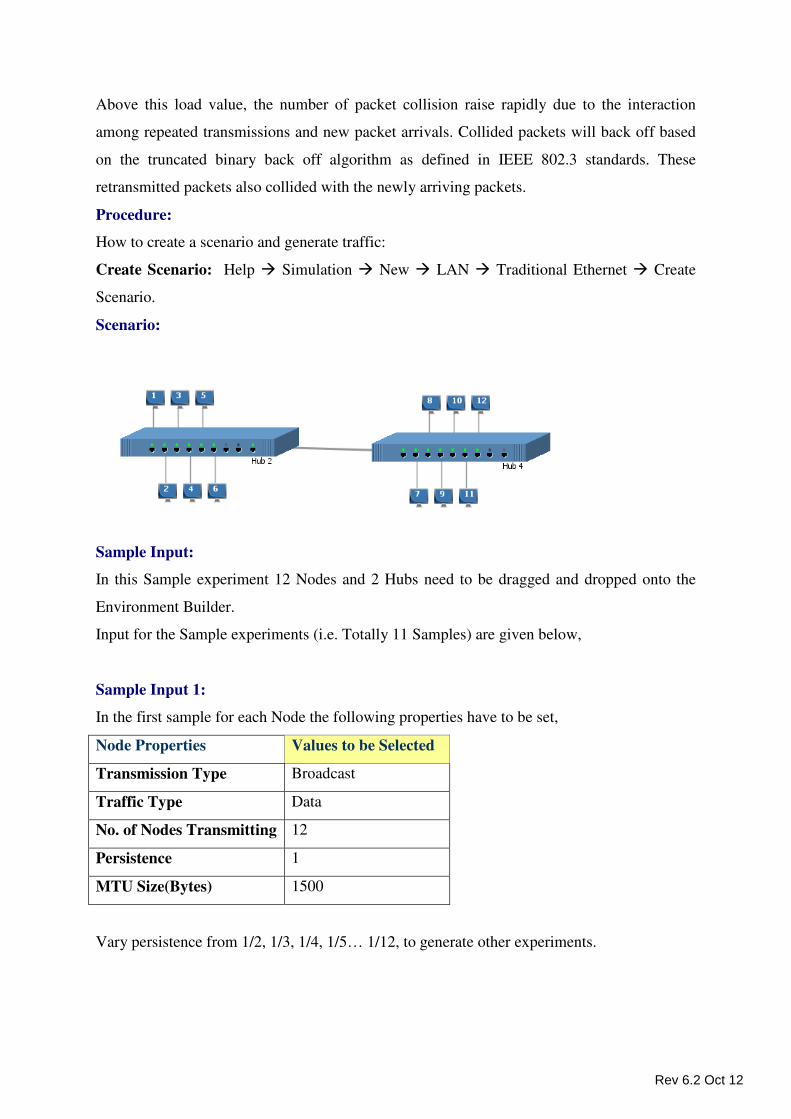
Scenario:
Sample Input:
In this Sample experiment 12 Nodes and 2 Hubs need to be dragged and dropped onto the
Environment Builder.
Input for the Sample experiments (i.e. Totally 11 Samples) are given below,
Sample Input 1:
In the first sample for each Node the following properties have to be set,
Node Properties Values to be Selected
Transmission Type Broadcast
Traffic Type Data
No. of Nodes Transmitting 12
Persistence 1
MTU Size(Bytes) 1500
Vary persistence from 1/2, 1/3, 1/4, 1/5… 1/12, to generate other experiments.
Rev 6.2 Oct 12
Data Input Configuration: (This window is obtained when Data is selected in Traffic
Type):
Packet Size Distribution Constant
Application Data Size (Bytes) 1472
Inter Arrival Time Distribution Exponential
Mean Inter Arrival Time(Micro Sec) 1000
Hub Properties common for Hub1 and Hub2:
Hub Properties Values to be Selected
Data Rate(Mbps) 10
Error Rate (bit error rate) No error
Physical Medium Twisted Pair
Simulation Time - 10 Sec
(Note: The Simulation Time can be selected only after the following two tasks,
• Set the properties for the Nodes & The Hub
• Click on the Validate & Simulate button).
Output:
After simulation of each experiment, click on the network statistics and note down the user
level throughput values. Open an excel sheet and plot a graph for these noted values against
their respective persistence values.
Rev 6.2 Oct 12
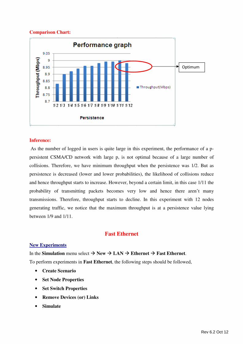
Comparison Chart:
Inference:
As the number of logged in users is quite large in this experiment, the performance of a p-
persistent CSMA/CD network with large p, is not optimal because of a large number of
collisions. Therefore, we have minimum throughput when the persistence was 1/2. But as
persistence is decreased (lower and lower probabilities), the likelihood of collisions reduce
and hence throughput starts to increase. However, beyond a certain limit, in this case 1/11 the
probability of transmitting packets becomes very low and hence there aren’t many
transmissions. Therefore, throughput starts to decline. In this experiment with 12 nodes
generating traffic, we notice that the maximum throughput is at a persistence value lying
between 1/9 and 1/11.
Fast Ethernet
New Experiments
In the Simulation menu select � New � LAN � Ethernet � Fast Ethernet.
To perform experiments in Fast Ethernet, the following steps should be followed,
• Create Scenario
• Set Node Properties
• Set Switch Properties
• Remove Devices (or) Links
• Simulate
Optimum
Rev 6.2 Oct 12
Create Scenario
Adding Switch - Click on the Switch icon and drag it onto the environment builder. By
default a Switch consists of eight ports.
Adding Node -
• Click on the Node icon and drag and drop it on the Switch.
• Nodes cannot be connected directly to each other because an intermediate
connecting component (such as Switch) is required.
A Node cannot be placed on another Node. A Node cannot float without a connection. It has
to be dragged and placed on any component.
Establishing Connections between two Switches - Click the two devices to connect
them. These two devices are connected via a Link.
Set Node Properties
Right Click on the appropriate node to select Properties. Inside the properties’ window click
on Application 1 to modify its properties.
Transmission Type
This indicates the type of transmission made by this session, either Broadcast or Point to
Point.
Destination
This property indicates the Destination Node.
Traffic Type
This property indicates the type of traffic. The traffic can either be Voice or Data.
Voice
Codec
Codec is the component of any voice system that translates between analog speech and
the bits used to transmit them. Every codec transmits a burst of data in a packet that can
be reconstructed into voice. Five different standards of voice codec’s are given which can
be selected depending on the variations required.
Service Type
• CBR - CBR stands for Constant Bit Rate. Packets of constant size are generated at
constant inter arrival times.
• VBR - VBR stands for Variable Bit Rate. The two types of Suppression Model that
can be selected are,
• Deterministic
Rev 6.2 Oct 12
• Markov Chain
Click OK to accept the user entered values. Click on the close button at the top
right corner to exit the screen.
Data
Packet Size
Distribution: The options available for distribution are,
• Constant
• Exponential
Mean Packet Size (Bytes): Sets the size of the packets being generated by the chosen
distribution. The ranges of values that can be entered are between 65 to 1500 bytes. By
default 1500 bytes is entered.
Inter Arrival Time
This indicates the time gap between packets.
Distribution: The options available for distribution are,
• Constant
• Exponential
• Uniform
Mean Inter Arrival Time: Enter the average inter-arrival time between packets. A
lower inter-arrival time would lead to a higher generation rate and the vice versa. The
ranges of values that can be entered are between 1000 to 20000 Micro Sec. By default
20000 Micro Sec is entered.
Click OK to accept the user entered values. Click on the close button at the top right
corner to exit the screen.
Modifying/Viewing/Accepting Properties
On opening an already configured properties of an application the input fields will be
frozen (i.e. the input cannot be changed).To modify these values click on the Modify
button in the screen. Now the input value can be changed. Click on the Accept button,
the modified values will be saved.
This View button is enabled once the Accept Button is clicked. To view the given
values, click on the View button.
Set Switch Properties
Right click on the appropriate Switch and click Properties.
Device Id - This property is a value that is generated automatically. The Id generated is a
unique one.
Priority - Priority level can be set between 1 and 65536. The default value is “32768”.
Switching Technique - There are 3 types of Switching Technique, they are,
Rev 6.2 Oct 12
• Store and Forward.
• Cut Through.
• Fragment Free.
Port Properties - The Port Properties that are mentioned below are common to all the
Ports available in a Switch.
Connected to - This property shows gives the Node number that is connected to that Port.
If no Node is connected then it is mentioned as ‘free’.
Communication - This property defines the communication mode of the network. By
default, a Switch network works in full duplex, hence this cannot be changed.
Data Rate - This property defines the rate at which the network transmits data. The option
available is 100 Mbps which indicates 100 Mega Bits per Second.
Error Rate - This property defines the rate of the error at which the data is affected in the
network. Options available are,
• No Error indicates No Error in every bit that is transmitted. This is the default
value found corresponding to Error Rate.
• 10^-6 indicates one error in every 1,000,000 bits transmitted.
• 10^-7 indicates one error in every 10,000,000 bits transmitted.
• 10^-8 indicates one error in every 100,000,000 bits transmitted.
• 10^-9 indicates one error in every 1000,000,000 bits transmitted.
Physical Medium - This property defines the type of Physical Medium that is used in the
network. The option available is Twisted Pair.
Buffer Size (MB) - This property specifies size of the buffer for that port on Switch.
Options available are � “1, 2, 3, 4 and 5”. Default value is 1MB.
MAC Address - MAC Address is an Address that is obtained automatically.
State - This property specifies the blocked/forward state of the port on Switch.
STP Cost - The value that is available next to STP Cost 19, since Data Rate is 100 Mbps
Remove Devices (or) Links
Remove Link - Right click on the appropriate Link and click Remove.
Remove Node - Right click on the appropriate Node and click Remove.
Remove Switch - Right click on the appropriate Switch and click Remove.
Rev 6.2 Oct 12
Note -
• If a Node transmitting data is removed, all traffic originating from this Node is also
deleted.
• In cases where the Switch is in a network (connected to other Switch), firstly the
connection need to be removed. Subsequently the Switch can be removed.
Simulate - After creating the Scenario the following steps need to be followed,
• Click on Validate button.
• Click on Simulate button.
• Select the Simulation End Time and then Click on “OK” button to start the
Simulation.
NetSim - Fast Ethernet
Sample Experiments - User can understand the internal working of Fast Ethernet through
these sample experiments. Each sample experiment covers:
• Procedure
• Sample Inputs
• Output
• Comparison chart
• Inference
Index Objective
Experiment 1
Compare the performance of Store and Forward, Cut Through and
Fragment Free switching techniques in an error prone switched
network.
Experiment 2 Study the working of the spanning tree algorithm by varying the
priority among the switches.
Sample Experiment 1
Objective:
Compare the performance of Store and Forward, Cut Through and Fragment Free switching
techniques in an error prone switched network.
Rev 6.2 Oct 12
Theory:
Refer NetSim basics on Switches
Procedure:
How to Create Scenario & Generate Traffic:
Please navigate through the below given path to,
o Create Scenario: “Help � NetSim Help � Simulation � New � LAN �
Ethernet � Fast Ethernet � Create Scenario”.
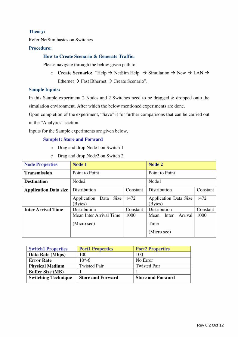
Sample Inputs:
In this Sample experiment 2 Nodes and 2 Switches need to be dragged & dropped onto the
simulation environment. After which the below mentioned experiments are done.
Upon completion of the experiment, “Save” it for further comparisons that can be carried out
in the “Analytics” section.
Inputs for the Sample experiments are given below,
Sample1: Store and Forward
o Drag and drop Node1 on Switch 1
o Drag and drop Node2 on Switch 2
Node Properties Node 1 Node 2
Transmission Point to Point Point to Point
Destination Node2 Node1
Application Data size Distribution Constant Distribution Constant
Application Data Size
(Bytes)
1472 Application Data Size
(Bytes)
1472
Inter Arrival Time
Distribution Constant Distribution Constant
Mean Inter Arrival Time
(Micro sec)
1000 Mean Inter Arrival
Time
(Micro sec)
1000
Switch1 Properties Port1 Properties Port2 Properties
Data Rate (Mbps) 100 100
Error Rate 10^-6 No Error
Physical Medium Twisted Pair Twisted Pair
Buffer Size (MB) 1 1
Switching Technique Store and Forward Store and Forward
Rev 6.2 Oct 12
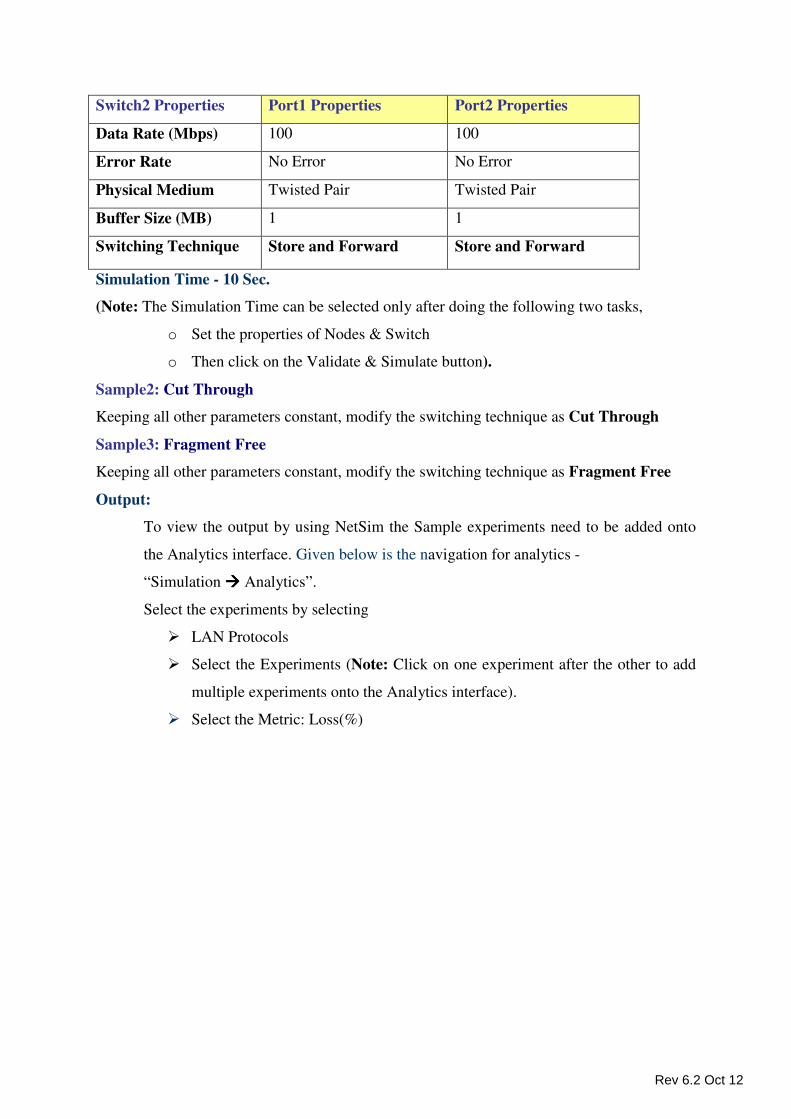
Switch2 Properties Port1 Properties Port2 Properties
Data Rate (Mbps) 100 100
Error Rate No Error No Error
Physical Medium Twisted Pair Twisted Pair
Buffer Size (MB) 1 1
Switching Technique Store and Forward Store and Forward
Simulation Time - 10 Sec.
(Note: The Simulation Time can be selected only after doing the following two tasks,
o Set the properties of Nodes & Switch
o Then click on the Validate & Simulate button).
Sample2: Cut Through
Keeping all other parameters constant, modify the switching technique as Cut Through
Sample3: Fragment Free
Keeping all other parameters constant, modify the switching technique as Fragment Free
Output:
To view the output by using NetSim the Sample experiments need to be added onto
the Analytics interface. Given below is the navigation for analytics -
“Simulation ���� Analytics”.
Select the experiments by selecting
� LAN Protocols
� Select the Experiments (Note: Click on one experiment after the other to add
multiple experiments onto the Analytics interface).
� Select the Metric: Loss(%)
Rev 6.2 Oct 12
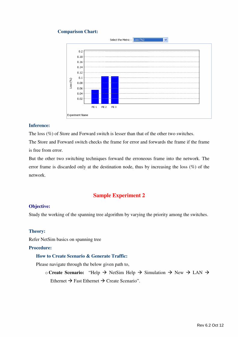
Comparison Chart:
Inference:
The loss (%) of Store and Forward switch is lesser than that of the other two switches.
The Store and Forward switch checks the frame for error and forwards the frame if the frame
is free from error.
But the other two switching techniques forward the erroneous frame into the network. The
error frame is discarded only at the destination node, thus by increasing the loss (%) of the
network.
Sample Experiment 2
Objective:
Study the working of the spanning tree algorithm by varying the priority among the switches.
Theory:
Refer NetSim basics on spanning tree
Procedure:
How to Create Scenario & Generate Traffic:
Please navigate through the below given path to,
o Create Scenario: “Help � NetSim Help � Simulation � New � LAN �
Ethernet � Fast Ethernet � Create Scenario”.
Rev 6.2 Oct 12
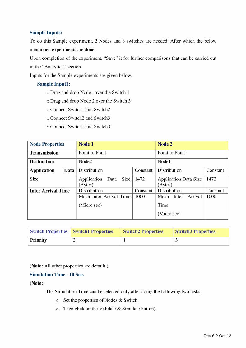
Sample Inputs:
To do this Sample experiment, 2 Nodes and 3 switches are needed. After which the below
mentioned experiments are done.
Upon completion of the experiment, “Save” it for further comparisons that can be carried out
in the “Analytics” section.
Inputs for the Sample experiments are given below,
Sample Input1:
o Drag and drop Node1 over the Switch 1
o Drag and drop Node 2 over the Switch 3
o Connect Switch1 and Switch2
o Connect Switch2 and Switch3
o Connect Switch1 and Switch3
Node Properties Node 1 Node 2
Transmission Point to Point Point to Point
Destination Node2 Node1
Application Data
Size
Distribution Constant Distribution Constant
Application Data Size
(Bytes)
1472 Application Data Size
(Bytes)
1472
Inter Arrival Time
Distribution Constant Distribution Constant
Mean Inter Arrival Time
(Micro sec)
1000 Mean Inter Arrival
Time
(Micro sec)
1000
Switch Properties Switch1 Properties Switch2 Properties Switch3 Properties
Priority 2 1 3
(Note: All other properties are default.)
Simulation Time - 10 Sec.
(Note:
The Simulation Time can be selected only after doing the following two tasks,
o Set the properties of Nodes & Switch
o Then click on the Validate & Simulate button).
Rev 6.2 Oct 12
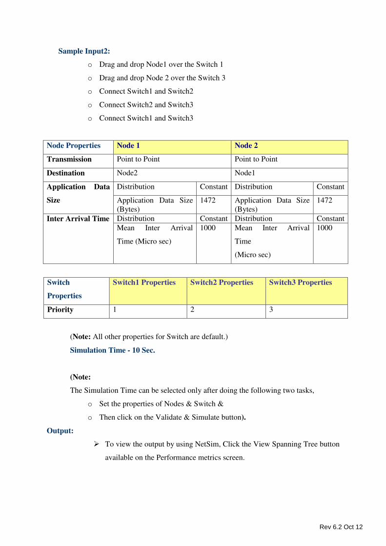
Sample Input2:
o Drag and drop Node1 over the Switch 1
o Drag and drop Node 2 over the Switch 3
o Connect Switch1 and Switch2
o Connect Switch2 and Switch3
o Connect Switch1 and Switch3
Node Properties Node 1 Node 2
Transmission Point to Point Point to Point
Destination Node2 Node1
Application Data
Size
Distribution Constant Distribution Constant
Application Data Size
(Bytes)
1472 Application Data Size
(Bytes)
1472
Inter Arrival Time
Distribution Constant Distribution Constant
Mean Inter Arrival
Time (Micro sec)
1000 Mean Inter Arrival
Time
(Micro sec)
1000
Switch
Properties
Switch1 Properties Switch2 Properties Switch3 Properties
Priority 1 2 3
(Note: All other properties for Switch are default.)
Simulation Time - 10 Sec.
(Note:
The Simulation Time can be selected only after doing the following two tasks,
o Set the properties of Nodes & Switch &
o Then click on the Validate & Simulate button).
Output:
� To view the output by using NetSim, Click the View Spanning Tree button
available on the Performance metrics screen.
Rev 6.2 Oct 12
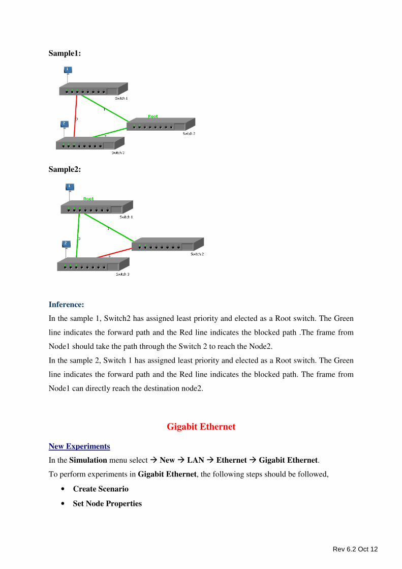
Sample1:
Sample2:
Inference:
In the sample 1, Switch2 has assigned least priority and elected as a Root switch. The Green
line indicates the forward path and the Red line indicates the blocked path .The frame from
Node1 should take the path through the Switch 2 to reach the Node2.
In the sample 2, Switch 1 has assigned least priority and elected as a Root switch. The Green
line indicates the forward path and the Red line indicates the blocked path. The frame from
Node1 can directly reach the destination node2.
Gigabit Ethernet
New Experiments
In the Simulation menu select � New � LAN � Ethernet � Gigabit Ethernet.
To perform experiments in Gigabit Ethernet, the following steps should be followed,
• Create Scenario
• Set Node Properties
Rev 6.2 Oct 12
• Set Switch Properties
• Remove Devices (or) Links
• Simulate
Create Scenario
Adding Switch - Click on the Switch icon and drag it onto the environment builder. By
default a Switch consists of eight ports.
Adding Node -
• Click on the Node icon and drag and drop it on the Switch.
• Nodes cannot be connected directly to each other because an intermediate connecting
component (such as Switch) is required.
A Node cannot be placed on another Node. A Node cannot float without a connection. It has to
be dragged and placed on any component.
Establishing Connections between two Switches - Click the two devices to connect
them. These two devices are connected via a Link.
Set Node Properties
Right Click on the appropriate node to select Properties. Inside the properties’ window click
on Application 1 to modify its properties.
Transmission Type
This indicates the type of transmission made by this session, either Broadcast or Point to
Point.
Destination
This property indicates the Destination Node.
Traffic Type
This property indicates the type of traffic. The traffic can either be Voice or Data.
Voice
Codec
Codec is the component of any voice system that translates between analog speech and
the bits used to transmit them. Every codec transmits a burst of data in a packet that can
be reconstructed into voice. Five different standards of voice codec’s are given which can
be selected depending on the variations required.
Service Type
• CBR - CBR stands for Constant Bit Rate. Packets of constant size are generated at
constant inter arrival times.
Rev 6.2 Oct 12
• VBR - VBR stands for Variable Bit Rate. The two types of Suppression Model that
can be selected are,
• Deterministic
• Markov Chain
Click OK to accept the user entered values. Click on the close button at the top right
corner to exit the screen.
Data
Packet Size
Distribution: The options available for distribution are,
• Constant
• Exponential
Mean Packet Size (Bytes): Sets the size of the packets being generated by the chosen
distribution. The range of values that can be entered are between 65 to 1500 bytes. By
default 1500 bytes is entered.
Inter Arrival Time
This indicates the time gap between packets.
Distribution: The options available for distribution are,
• Constant
• Exponential
• Uniform
Mean Inter Arrival Time: Enter the average inter-arrival time between packets. A
lower inter-arrival time would lead to a higher generation rate and the vice versa. The
range of values that can be entered are between 1000 to 20000 Micro Sec. By default
20000 Micro Sec is entered.
Click OK to accept the user entered values. Click on the close button at the top right
corner to exit the screen.
Modifying/Viewing/Accepting Properties
On opening an already configured properties of an application the input fields will be
frozen (i.e. the input cannot be changed).To modify these values click on the Modify
button in the screen. Now the input value can be changed. Click on the Accept button,
the modified values will be saved.
This View button is enabled once the Accept Button is clicked. To view the given
values, click on the View button.
Set Switch Properties
Right click on the appropriate Switch and click Properties.
Device Id - This property is a value that is generated automatically. The Id generated is a
unique one.
Rev 6.2 Oct 12
Priority - Priority level can be set between 1 and 65536. The default value is “32768”.
Switching Technique - There are 3 types of Switching Technique, they are,
• Store and Forward.
• Cut Through.
• Fragment Free.
Port Properties - The Port Properties that are mentioned below are common to all the
Ports available in a Switch.
Connected to - This property shows gives the Node number that is connected to that Port.
If no Node is connected then it is mentioned as ‘free’.
Communication - This property defines the communication mode of the network. By
default, a Switch network works in full duplex, hence this cannot be changed.
Data Rate - This property defines the rate at which the network transmits data. The option
available is 100 Mbps which indicates 1000 Mega Bits per Second.
Error Rate - This property defines the rate of the error at which the data is affected in the
network. Options available are,
• No Error indicates No Error in every bit that is transmitted. This is the
default value found corresponding to Error Rate.
• 10^-6 indicates one error in every 1,000,000 bits transmitted.
• 10^-7 indicates one error in every 10,000,000 bits transmitted.
• 10^-8 indicates one error in every 100,000,000 bits transmitted.
• 10^-9 indicates one error in every 1000,000,000 bits transmitted.
Physical Medium - This property defines the type of Physical Medium that is used in
the network. The option available is Twisted Pair.
Buffer Size (MB) - This property specifies size of the buffer for that port on Switch.
Options available are � “1, 2, 3, 4 and 5”. Default value is 1MB.
MAC Address - MAC Address is an Address that is obtained automatically.
State - This property specifies the blocked/forward state of the port on Switch.
STP Cost - The value that is available next to STP Cost 19, since Data Rate is 1000
Mbps
Rev 6.2 Oct 12
Remove Devices (or) Links
Remove Link - Right click on the appropriate Link and click Remove.
Remove Node - Right click on the appropriate Node and click Remove.
Remove Switch - Right click on the appropriate Switch and click Remove.
Note -
• If a Node transmitting data is removed, all traffic originating from this Node is also
deleted.
• In cases where the Switch is in a network (connected to other Switch), firstly the
connection need to be removed. Subsequently the Switch can be removed.
Simulate - After creating the Scenario the following steps need to be followed,
• Click on Validate button.
• Click on Simulate button.
• Select the Simulation End Time and then Click on “OK” button to start the
Simulation.
MANET
New Experiments
In the Simulation menu select � New � LAN �MANET
To perform experiments in MANET, the following steps should be followed,
• Create Scenario
• Set Node Properties
• Remove Devices
• Simulate
Create Scenario
Adding Node -
• Click on the Node icon and drag and drop it in side the Environment (i.e.
Visibility Range - The systems can move and communicate in this range only).
• Nodes are needed to find the Route to data, and then it starts its transmission through
path.
A Node cannot be placed on another Node. A Node cannot float outside the
Environment. It has to be dragged and placed inside the Visibility Range.
Rev 6.2 Oct 12
Set Node Properties
Right Click on the appropriate node to select Properties. Inside the properties’ window click
on Application 1 to modify its properties.
Transmission Type
This indicates the type of transmission made by this session, Point to Point.
Destination
This property indicates the Destination Node.
Traffic Type
This property indicates the type of traffic. The traffic can either be Voice or Data.
Voice
Codec
Codec is the component of any voice system that translates between analog speech and the
bits used to transmit them. Every codec transmits a burst of data in a packet that can be
reconstructed into voice. Three different standards of voice codec’s are given which can be
selected depending on the variations required.
Service Type
• CBR - CBR stands for Constant Bit Rate. Packets of constant size are generated at
constant inter arrival times.
• VBR - VBR stands for Variable Bit Rate. The two types of Suppression Model that
can be selected are,
• Deterministic
• Markov Chain
• Success Ratio (%)
Click OK to accept the user entered values. Click on the close button at the top
right corner to exit the screen.
Data
Packet Size
Distribution: The options available for distribution are,
• Constant
• Exponential
Mean Packet Size (Bytes): Sets the size of the packets being generated by the Constant
distribution. The ranges of values that can be entered are between 10 to 10000 bytes. By
default 1472 bytes is entered.
Inter Arrival Time
This indicates the time gap between packets.
Distribution: The options available for distribution are,
Rev 6.2 Oct 12
• Exponential
• Uniform
• Constant
Mean Inter Arrival Time: Enter the average inter-arrival time between packets. A lower
inter-arrival time would lead to a higher generation rate and the vice versa. The ranges of
values that can be entered are between 1000 to 20000 Micro Sec. By default 20000 Micro
Sec is entered.
Data Link Layer
Protocol- A default value has been coded in; hence no change can be made.
MAC Address - A default value has been coded in, hence no change can be made.
RTS Threshold (Bytes) - This property is to allow the node to enable/disable the
RTS/CTS mechanism. By default the value that is available is 2347 Bytes. Limit
ranges from 0 to 2347 Bytes.
Retry Limit - Indicate the number of attempts that can be made by a frame. This
varies from 1 to 7. By default the Retry Limit value is 7.
MTU- A default value has been coded in, hence no change can be made.
Physical Layer
Transmitter Power (milli watts) - This property defines the power level of the
Node. By default the value for Transmitter Power is 100 milli watts.
This View button is enabled once the Accept Button is clicked. To view the given
values, click on the View button.
Click OK to accept the user entered values. Click on the close button at the top right
corner to exit the screen.
Modifying/Viewing/Accepting Properties
On opening an already configured properties of an application the input fields will be
frozen (i.e. the input cannot be changed).To modify these values click on the Modify
button in the screen. Now the input value can be changed. Click on the Accept button,
the modified values will be saved.
This View button is enabled once the Accept Button is clicked. To view the given
values, click on the View button.
Set Environment Properties
Right click in side of the on the Environment and click Properties.
Mobility model
Mobility - A default value has been coded in; hence no change can be made.
Rev 6.2 Oct 12
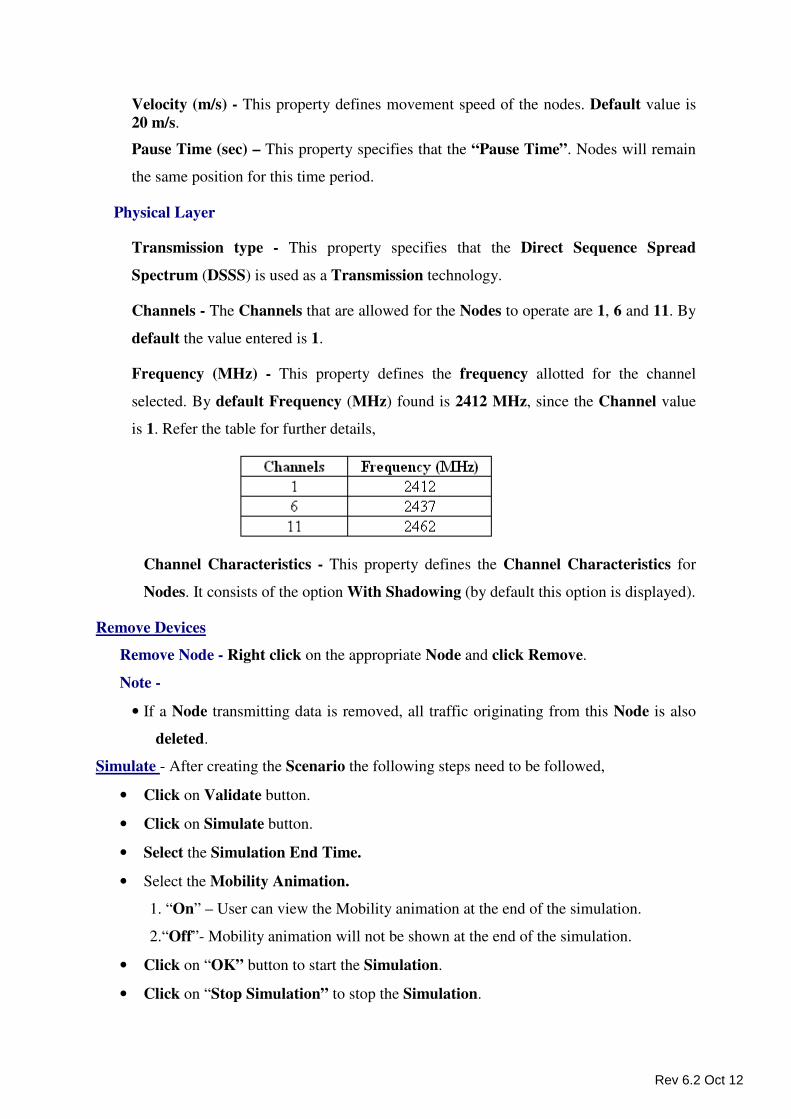
Velocity (m/s) - This property defines movement speed of the nodes. Default value is
20 m/s.
Pause Time (sec) – This property specifies that the “Pause Time”. Nodes will remain
the same position for this time period.
Physical Layer
Transmission type - This property specifies that the Direct Sequence Spread
Spectrum (DSSS) is used as a Transmission technology.
Channels - The Channels that are allowed for the Nodes to operate are 1, 6 and 11. By
default the value entered is 1.
Frequency (MHz) - This property defines the frequency allotted for the channel
selected. By default Frequency (MHz) found is 2412 MHz, since the Channel value
is 1. Refer the table for further details,
Channel Characteristics - This property defines the Channel Characteristics for
Nodes. It consists of the option With Shadowing (by default this option is displayed).
Remove Devices
Remove Node - Right click on the appropriate Node and click Remove.
Note -
• If a Node transmitting data is removed, all traffic originating from this Node is also
deleted.
Simulate - After creating the Scenario the following steps need to be followed,
• Click on Validate button.
• Click on Simulate button.
• Select the Simulation End Time.
• Select the Mobility Animation.
1. “On” – User can view the Mobility animation at the end of the simulation.
2.“Off”- Mobility animation will not be shown at the end of the simulation.
• Click on “OK” button to start the Simulation.
• Click on “Stop Simulation” to stop the Simulation.
Rev 6.2 Oct 12
NetSim - MANET
Sample Experiments - User can understand the internal working of Dynamic Source
Routing through these sample experiments. Each sample experiment covers:
• Procedure
• Sample Inputs
• Output
• Comparison chart
• Inference
Index Objective
MANET -
Experiment 1
To create scenario and study the performance of MANET mobility
model using NetSim simulation.
.
Sample Experiment 1
Objective:
To create scenario and study the performance of MANET mobility model using NetSim
simulation.
Introduction:
In Random waypoint model, nodes will move freely, and remain in the same position for
some time, which is called “Pause Time”, and then it will choose another random position
and it will move towards that position with a given velocity. For further details refer Basics
� LAN Protocols � MANET�Mobility.
Procedure:
How to Create Scenario & Generate Traffic:
Please refer,
o Create Scenario: “Help � NetSim Help F1�Simulation � New � LAN �
MANET � Create Scenario”.
Rev 6.2 Oct 12
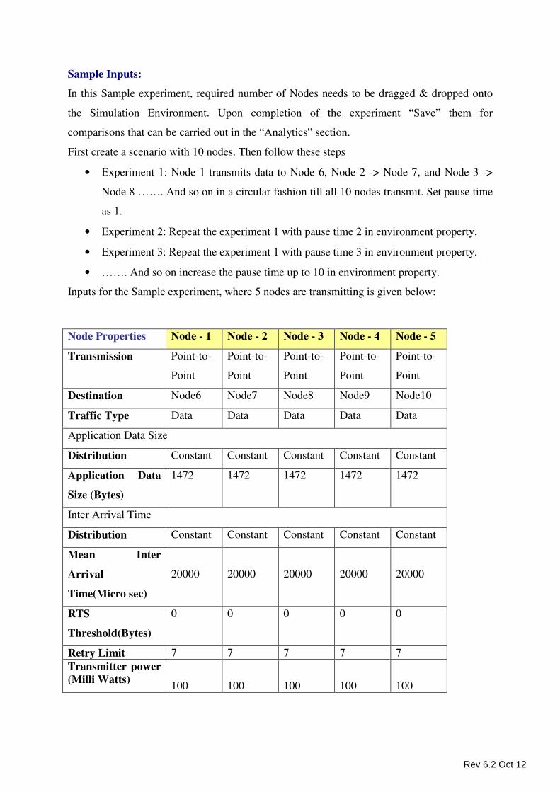
Sample Inputs:
In this Sample experiment, required number of Nodes needs to be dragged & dropped onto
the Simulation Environment. Upon completion of the experiment “Save” them for
comparisons that can be carried out in the “Analytics” section.
First create a scenario with 10 nodes. Then follow these steps
• Experiment 1: Node 1 transmits data to Node 6, Node 2 -> Node 7, and Node 3 ->
Node 8 ……. And so on in a circular fashion till all 10 nodes transmit. Set pause time
as 1.
• Experiment 2: Repeat the experiment 1 with pause time 2 in environment property.
• Experiment 3: Repeat the experiment 1 with pause time 3 in environment property.
• ……. And so on increase the pause time up to 10 in environment property.
Inputs for the Sample experiment, where 5 nodes are transmitting is given below:
Node Properties Node - 1 Node - 2 Node - 3 Node - 4 Node - 5
Transmission Point-to-
Point
Point-to-
Point
Point-to-
Point
Point-to-
Point
Point-to-
Point
Destination Node6 Node7 Node8 Node9 Node10
Traffic Type Data Data Data Data Data
Application Data Size
Distribution Constant Constant Constant Constant Constant
Application Data
Size (Bytes)
1472 1472 1472 1472 1472
Inter Arrival Time
Distribution Constant Constant Constant Constant Constant
Mean Inter
Arrival
Time(Micro sec)
20000
20000
20000
20000
20000
RTS
Threshold(Bytes)
0 0 0 0 0
Retry Limit 7 7 7 7 7
Transmitter power
(Milli Watts)
100
100
100
100
100
Rev 6.2 Oct 12
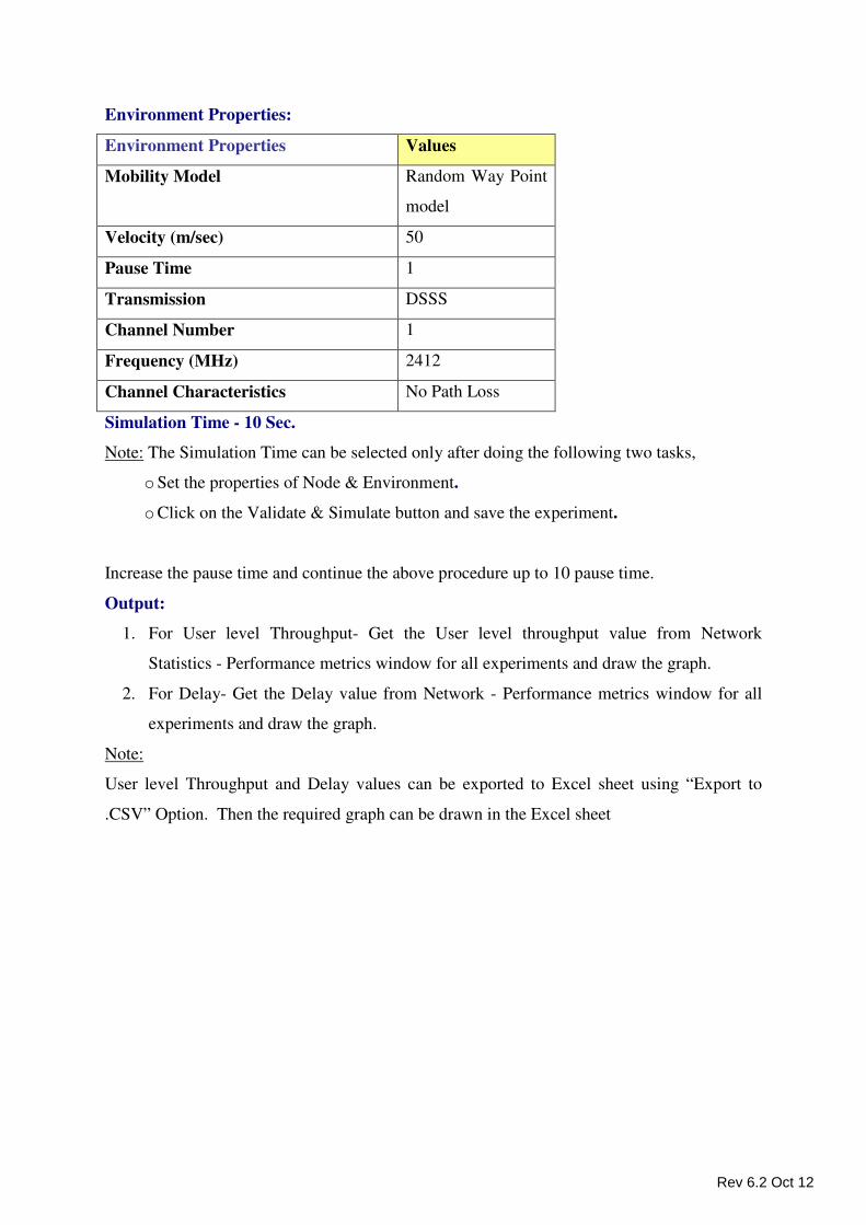
Environment Properties:
Environment Properties Values
Mobility Model Random Way Point
model
Velocity (m/sec) 50
Pause Time 1
Transmission DSSS
Channel Number 1
Frequency (MHz) 2412
Channel Characteristics No Path Loss
Simulation Time - 10 Sec.
Note: The Simulation Time can be selected only after doing the following two tasks,
o Set the properties of Node & Environment.
o Click on the Validate & Simulate button and save the experiment.
Increase the pause time and continue the above procedure up to 10 pause time.
Output:
1. For User level Throughput- Get the User level throughput value from Network
Statistics - Performance metrics window for all experiments and draw the graph.
2. For Delay- Get the Delay value from Network - Performance metrics window for all
experiments and draw the graph.
Note:
User level Throughput and Delay values can be exported to Excel sheet using “Export to
.CSV” Option. Then the required graph can be drawn in the Excel sheet
Rev 6.2 Oct 12
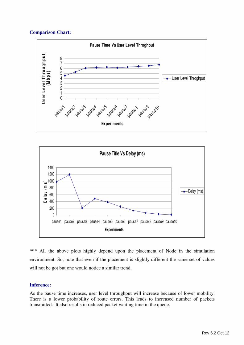
Comparison Chart:
Pause Time Vs User Level Throghput
012345678
paus
e1
pause2
pause3
pause4
pause5
pause6
paus
e7
pause 8
pause9
pause10
Experiments
Us
er
Le
ve
l T
hro
ug
hp
ut
(Mb
ps
)
User Level Throghput
*** All the above plots highly depend upon the placement of Node in the simulation
environment. So, note that even if the placement is slightly different the same set of values
will not be got but one would notice a similar trend.
Inference:
As the pause time increases, user level throughput will increase because of lower mobility.
There is a lower probability of route errors. This leads to increased number of packets
transmitted. It also results in reduced packet waiting time in the queue.
Pause Title Vs Delay (ms)
0
200
400
600
800
1000
1200
1400
pause1 pause2 pause3 pause4 pause5 pause6 pause7 pause 8 pause9 pause10
Experiments
De
lay
(m
s)
Delay (ms)
Rev 6.2 Oct 12
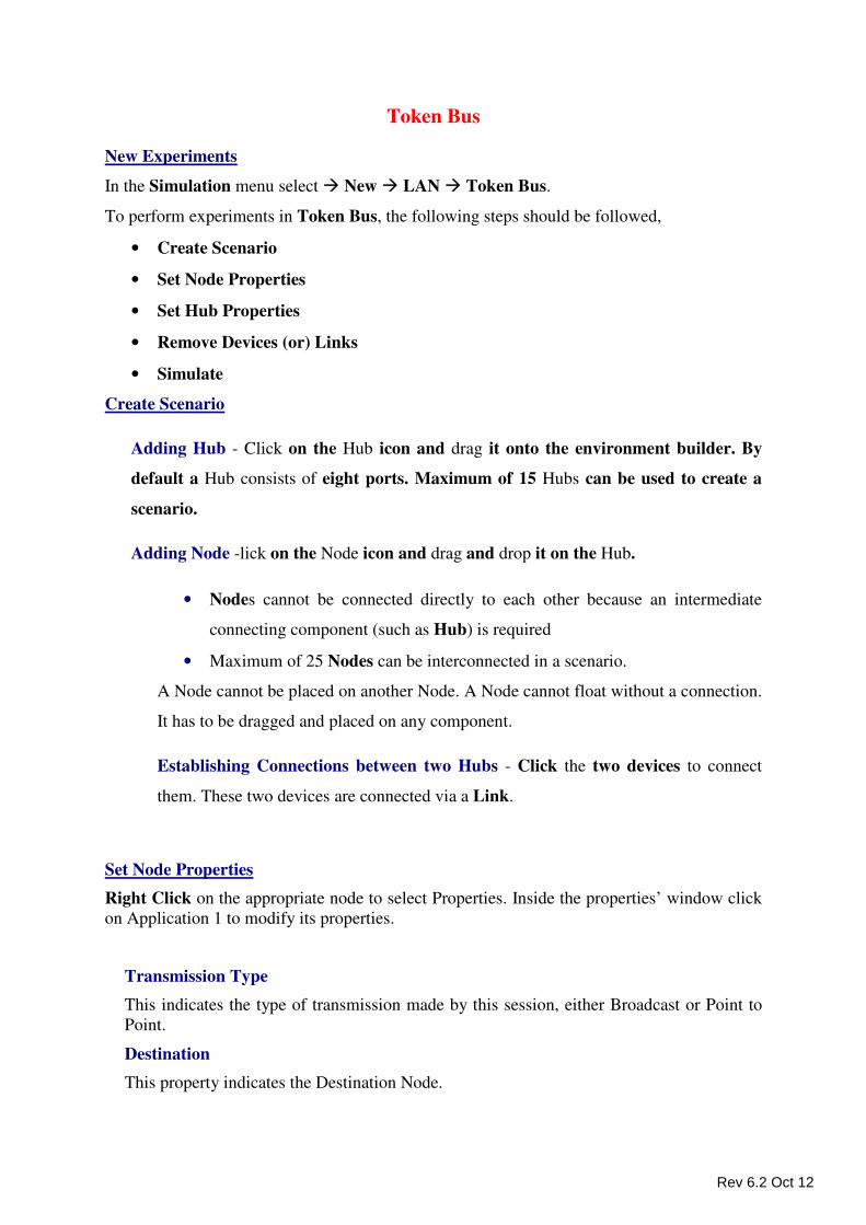
Token Bus
New Experiments
In the Simulation menu select � New � LAN � Token Bus.
To perform experiments in Token Bus, the following steps should be followed,
• Create Scenario
• Set Node Properties
• Set Hub Properties
• Remove Devices (or) Links
• Simulate
Create Scenario
Adding Hub - Click on the Hub icon and drag it onto the environment builder. By
default a Hub consists of eight ports. Maximum of 15 Hubs can be used to create a
scenario.
Adding Node -lick on the Node icon and drag and drop it on the Hub.
• Nodes cannot be connected directly to each other because an intermediate
connecting component (such as Hub) is required
• Maximum of 25 Nodes can be interconnected in a scenario.
A Node cannot be placed on another Node. A Node cannot float without a connection.
It has to be dragged and placed on any component.
Establishing Connections between two Hubs - Click the two devices to connect
them. These two devices are connected via a Link.
Set Node Properties
Right Click on the appropriate node to select Properties. Inside the properties’ window click
on Application 1 to modify its properties.
Transmission Type
This indicates the type of transmission made by this session, either Broadcast or Point to
Point.
Destination
This property indicates the Destination Node.
Rev 6.2 Oct 12
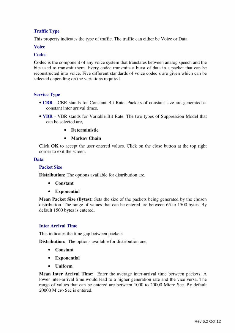
Traffic Type
This property indicates the type of traffic. The traffic can either be Voice or Data.
Voice
Codec
Codec is the component of any voice system that translates between analog speech and the
bits used to transmit them. Every codec transmits a burst of data in a packet that can be
reconstructed into voice. Five different standards of voice codec’s are given which can be
selected depending on the variations required.
Service Type
• CBR - CBR stands for Constant Bit Rate. Packets of constant size are generated at
constant inter arrival times.
• VBR - VBR stands for Variable Bit Rate. The two types of Suppression Model that
can be selected are,
• Deterministic
• Markov Chain
Click OK to accept the user entered values. Click on the close button at the top right
corner to exit the screen.
Data
Packet Size
Distribution: The options available for distribution are,
• Constant
• Exponential
Mean Packet Size (Bytes): Sets the size of the packets being generated by the chosen
distribution. The range of values that can be entered are between 65 to 1500 bytes. By
default 1500 bytes is entered.
Inter Arrival Time
This indicates the time gap between packets.
Distribution : The options available for distribution are,
• Constant
• Exponential
• Uniform
Mean Inter Arrival Time: Enter the average inter-arrival time between packets. A
lower inter-arrival time would lead to a higher generation rate and the vice versa. The
range of values that can be entered are between 1000 to 20000 Micro Sec. By default
20000 Micro Sec is entered.
Rev 6.2 Oct 12
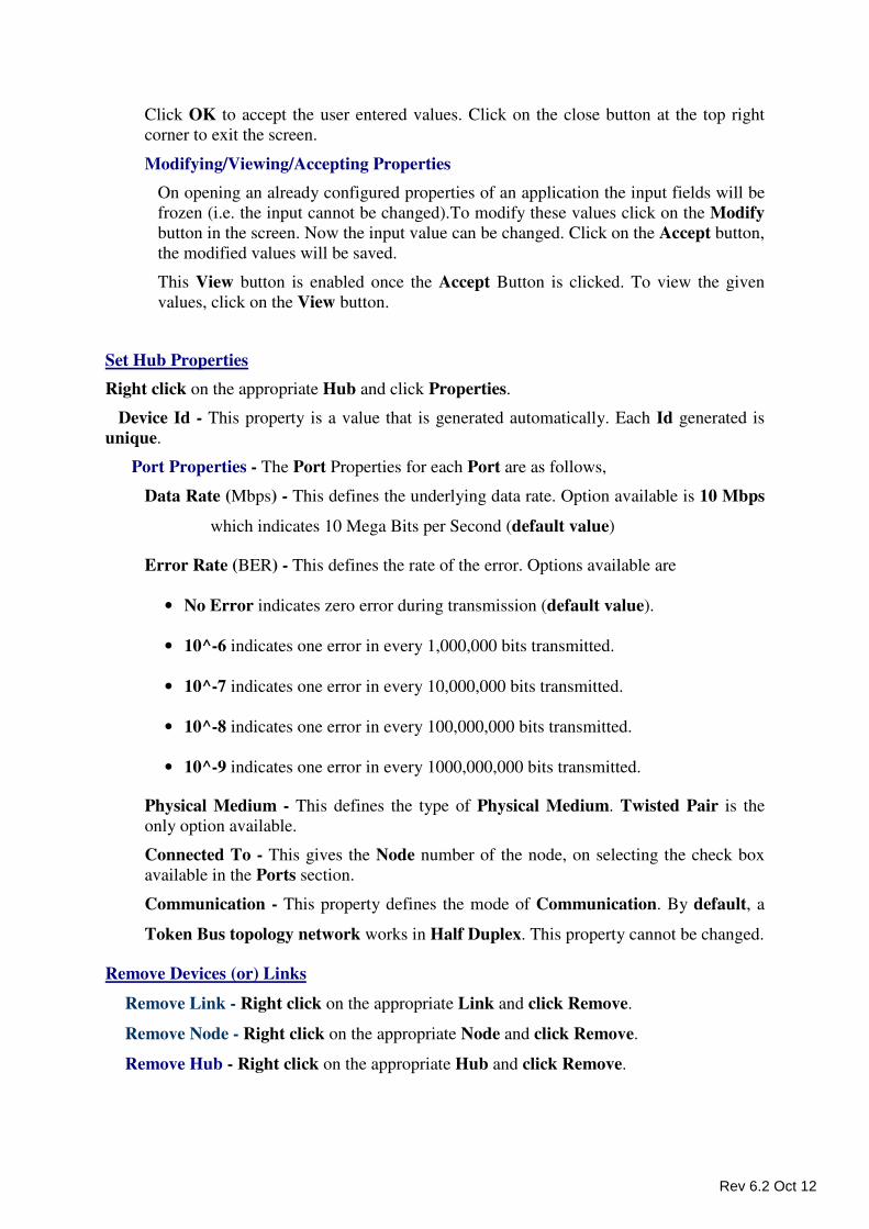
Click OK to accept the user entered values. Click on the close button at the top right
corner to exit the screen.
Modifying/Viewing/Accepting Properties
On opening an already configured properties of an application the input fields will be
frozen (i.e. the input cannot be changed).To modify these values click on the Modify
button in the screen. Now the input value can be changed. Click on the Accept button,
the modified values will be saved.
This View button is enabled once the Accept Button is clicked. To view the given
values, click on the View button.
Set Hub Properties
Right click on the appropriate Hub and click Properties.
Device Id - This property is a value that is generated automatically. Each Id generated is
unique.
Port Properties - The Port Properties for each Port are as follows,
Data Rate (Mbps) - This defines the underlying data rate. Option available is 10 Mbps
which indicates 10 Mega Bits per Second (default value)
Error Rate (BER) - This defines the rate of the error. Options available are
• No Error indicates zero error during transmission (default value).
• 10^-6 indicates one error in every 1,000,000 bits transmitted.
• 10^-7 indicates one error in every 10,000,000 bits transmitted.
• 10^-8 indicates one error in every 100,000,000 bits transmitted.
• 10^-9 indicates one error in every 1000,000,000 bits transmitted.
Physical Medium - This defines the type of Physical Medium. Twisted Pair is the
only option available.
Connected To - This gives the Node number of the node, on selecting the check box
available in the Ports section.
Communication - This property defines the mode of Communication. By default, a
Token Bus topology network works in Half Duplex. This property cannot be changed.
Remove Devices (or) Links
Remove Link - Right click on the appropriate Link and click Remove.
Remove Node - Right click on the appropriate Node and click Remove.
Remove Hub - Right click on the appropriate Hub and click Remove.
Rev 6.2 Oct 12
Note -
• If a Node transmitting data is removed, all traffic originating from this Node is also
deleted.
• In cases where the Hub is in a network (connected to other Hub), firstly the
connection need to be removed. Subsequently the Hub can be removed
Simulate - After creating the Scenario the following steps need to be followed,
• Click on Validate button.
• Click on Simulate button.
• Select the Simulation End Time and then Click on “OK” button to start the
Simulation.
Token Ring
New Experiments
In the Simulation menu select � New � LAN � Token Ring.
To perform experiments in Token Ring, the following steps should be followed,
• Create Scenario
• Set Node Properties
• Set Concentrator Properties
• Remove Devices (or) Links
• Simulate
Create Scenario
Adding Concentrator - Click on the Concentrator icon and drag it onto the environment
builder. By default a Concentrator consists of eight ports.
Adding Node -
• Click on the Node icon and drag and drop it on the Concentrator.
• Nodes cannot be connected directly to each other because an intermediate
connecting component (such as Concentrator) is required.
A Node cannot be placed on another Node. A Node cannot float without a connection.
It has to be dragged and placed on any component.
Establishing Connections between two Concentrators - Click the two devices to
connect them. These two devices are connected via a Link.
Rev 6.2 Oct 12
Set Node Properties
Right Click on the appropriate node to select Properties. Inside the properties’ window click
on Application 1 to modify its properties.
Transmission Type
This indicates the type of transmission made by this session, either Broadcast or Point to
Point.
Destination
This property indicates the Destination Node.
Traffic Type
This property indicates the type of traffic. The traffic can either be Voice or Data.
Voice
Codec
Codec is the component of any voice system that translates between analog speech
and the bits used to transmit them. Every codec transmits a burst of data in a packet
that can be reconstructed into voice. Five different standards of voice codec’s are
given which can be selected depending on the variations required.
Service Type
• CBR - CBR stands for Constant Bit Rate. Packets of constant size are
generated at constant inter arrival times.
• VBR - VBR stands for Variable Bit Rate. The two types of Suppression
Model that can be selected are,
• Deterministic
• Markov Chain
Click OK to accept the user entered values. Click on the close button at the top
right corner to exit the screen.
Data
Packet Size
Distribution: The options available for distribution are,
• Constant
• Exponential
Mean Packet Size (Bytes): Sets the size of the packets being generated by the
chosen distribution. The range of values that can be entered are between 65 to 1500
bytes. By default 1500 bytes is entered.
Rev 6.2 Oct 12
Inter Arrival Time
This indicates the time gap between packets.
Distribution : The options available for distribution are,
• Constant
• Exponential
• Uniform
Mean Inter Arrival Time: Enter the average inter-arrival time between packets. A
lower inter-arrival time would lead to a higher generation rate and the vice versa.
The range of values that can be entered are between 1000 to 20000 Micro Sec. By
default 20000 Micro Sec is entered.
Click OK to accept the user entered values. Click on the close button at the top right
corner to exit the screen.
Modifying/Viewing/Accepting Properties
On opening an already configured properties of an application the input fields will
be frozen (i.e. the input cannot be changed).To modify these values click on the
Modify button in the screen. Now the input value can be changed. Click on the
Accept button, the modified values will be saved.
This View button is enabled once the Accept Button is clicked. To view the given
values, click on the View button.
Set Concentrator Properties
Right click on the appropriate Concentrator and click Properties.
Device Id - This property is a value that is generated automatically. Each Id generated is
unique.
Port Properties - The Port Properties for each Port are as follows,
Data Rate (Mbps) - This defines the underlying data rate. Options available are 4 and
16 Mbps. By default the value available is 16 Mbps.
Error Rate (BER) - This defines the rate of the error. Options available are
• No Error indicates zero error during transmission (default value).
• 10^-6 indicates one error in every 1,000,000 bits transmitted.
• 10^-7 indicates one error in every 10,000,000 bits transmitted.
• 10^-8 indicates one error in every 100,000,000 bits transmitted.
• 10^-9 indicates one error in every 1000,000,000 bits transmitted.
Physical Medium - This defines the type of Physical Medium. Twisted Pair is the
only option available.
Rev 6.2 Oct 12
Connected To - This gives the Node number of the node, on selecting the check box
available in the Ports section.
Communication - This property defines the mode of Communication. By default, a
Token Bus topology network works in Half Duplex. This property cannot be
changed.
Remove Devices (or) Links
Remove Link - Right click on the appropriate Link and click Remove.
Remove Node - Right click on the appropriate Node and click Remove.
Remove Concentrator - Right click on the appropriate Concentrator and click
Remove.
Note -
• If a Node transmitting data is removed, all traffic originating from this Node is
also deleted.
• In cases where the Concentrator is in a network (connected to other
Concentrator), firstly the connection need to be removed. Subsequently the
Concentrator can be removed.
Simulate - After creating the Scenario the following steps need to be followed,
• Click on Validate button.
• Click on Simulate button.
• Select the Simulation End Time and then Click on “OK” button to start the
Simulation.
Wireless LAN - 802.11a
New Experiments
In the Simulation menu select � New � LAN � Ethernet � Wireless LAN ���� 802.11a.
To perform experiments in Wireless LAN, the following steps should be followed,
• Create Scenario
• Set Node Properties
• Set Access Point (AP) Properties
• Remove Devices (or) Links
• Simulate
Rev 6.2 Oct 12
Create Scenario
Adding Wireless AP - Click on the Wireless AP icon and drag it onto the environment
builder.
Adding Switch - Click on the Switch icon and drag it onto the environment builder. By
default a Switch consists of eight ports.
Adding Node -
• Click on the Node icon and drag and drop it on the Wireless AP.
• Nodes cannot be connected directly to each other because an intermediate
connecting component (such as Switch) is required.
• A Node cannot be placed on another Node. It has to be dragged and placed on any
connecting component.
Establishing Connections between Switch, Wireless AP and Nodes - Click the two
devices to connect them. These two devices are connected via a Link
Set Node Properties
Right Click on the appropriate node to select Properties. Inside the properties’ window click
on Application 1 to modify its properties.
Transmission Type
This indicates the type of transmission made by this session, either Broadcast or Point to
Point.
Destination
This property indicates the Destination Node.
Traffic Type
This property indicates the type of traffic. The traffic can either be Voice or Data.
Voice
Codec
Codec is the component of any voice system that translates between analog speech and
the bits used to transmit them. Every codec transmits a burst of data in a packet that can
be reconstructed into voice. Five different standards of voice codec’s are given which
can be selected depending on the variations required.
Service Type
• CBR - CBR stands for Constant Bit Rate. Packets of constant size are generated at
constant inter arrival times.
Rev 6.2 Oct 12
• VBR - VBR stands for Variable Bit Rate. The two types of Suppression Model that
can be selected are,
• Deterministic
• Markov Chain
Click OK to accept the user entered values. Click on the close button at the top right
corner to exit the screen.
Data
Packet Size
Distribution: The options available for distribution are,
• Constant
• Exponential
Mean Packet Size (Bytes): Sets the size of the packets being generated by the
chosen distribution. The range of values that can be entered are between 65 to 1500
bytes. By default 1500 bytes is entered.
Inter Arrival Time
This indicates the time gap between packets.
Distribution: The options available for distribution are,
• Constant
• Exponential
• Uniform
Mean Inter Arrival Time: Enter the average inter-arrival time between packets.
A lower inter-arrival time would lead to a higher generation rate and the vice versa.
The ranges of values that can be entered are between 1000 to 20000 Micro Sec. By
default 20000 Micro Sec is entered.
Click OK to accept the user entered values. Click on the close button at the top
right corner to exit the screen.
RTS Threshold (Bytes)
This is to allow the node to enable/disable the RTS/CTS mechanism. The valid value
ranges from “0 to 2347”. Default values are 0 bytes.
Retry Limit
This indicates the number of attempts that can be made by a frame. The option varies
from 1 to 7.
Modifying/Viewing/Accepting Properties
On opening an already configured properties of an application the input fields will be
frozen (i.e. the input cannot be changed).To modify these values click on the Modify
button in the screen. Now the input value can be changed. Click on the Accept button,
the modified values will be saved.
Rev 6.2 Oct 12
This View button is enabled once the Accept Button is clicked. To view the given
values, click on the View button.
Set Access Point (AP) Properties
Right click on the appropriate Access Point (AP) and click Properties. Options available
are,
Wireless Properties - Under Wireless Properties tab the options available are,
Connected To - This property defines the Wireless medium connected to the Access
Point (AP). A default value is already entered; hence no changes can be done.
Communication - This property defines the Communication mode of the network. By
default, a Wireless LAN network works in Half Duplex. This property cannot be
changed.
Data Link Layer - Under Data Link Layer the sub-options available are,
MAC Address - A default value has been coded in, hence no change can be made.
Buffer Size (MB) - This property defines the buffer capacity of the Wireless Port.
Options available are � “1, 2, 3, 4 and 5”. Default value is 5MB.
Retry Limit - Indicate the number of attempts that can be made by a frame. This varies
from 1 to 7. By default the Retry Limit value is 7.
RTS Threshold (Bytes) - This property is to allow the node to enable/disable the
RTS/CTS mechanism. By default the value that is available is 2347 Bytes. Limit
ranges from 0 to 2347 Bytes.
Physical Layer - Under Physical Layer the sub-options available are,
Standard - This property gives the standard that is followed for modeling Physical
Layer. By default the standard is IEEE 802.11a can be found next to this property.
Transmission type - This property specifies that the Orthogonal Frequency Division
Multiplexing (OFDM). OFDM is used as a Transmission technology.
Channels - The Channels that are allowed for the Access Points (AP) to operate are
36, 40, 44 and 48. By default the value entered is 36.
Frequency (MHz) - This property defines the frequency allotted for the channel
selected. By default Frequency (MHz) found is 5180 MHz, since the Channel value
is 36. Refer the table for further details,
Rev 6.2 Oct 12
Channels Frequency (MHz)
36 5180
40 5200
44 5220
48 5240
Transmitter Power (milli watts) - This property defines the power level of the Access
Points (AP). It ranges from 1 to 40 milli watts. By default the value for Transmitter
Power is 40 milli watts.
Channel Characteristics - This property defines the Channel Characteristics for
Access Point. It consists of the following options,
• Without Fading
• With Fading
• With Shadowing (by default this option is displayed)
Ethernet Port Properties - To set the properties of the Ethernet Port of access point
select the Ethernet Port Properties tab. Options available are,
Connected To - This property gives the Port number and the Switch number that the
Access Point (AP) is connected.
For E.g.: If the Port number is Port1 and the Switch number is Switch1, then,
Connected To � Port1 of Switch1.
Communication - This property defines the Communication mode of the network. By
default, the Switch to Wireless AP connectivity works in Full Duplex, hence the user
cannot change this property.
Data Link Layer - Under Data Link Layer the following sub-options are,
MAC Address - This field is filled up with a default value. Changes cannot be made.
Buffer Size (MB) - This property defines the Buffer Capacity of the Wireless Port.
Options available are � “1, 2, 3, 4 and 5”. Default value is 1MB.
Rev 6.2 Oct 12
Data Rate (Mbps) - This property defines the rate at which the link transmits data. By
default the Data Rate (Mbps) is 100. 100 Mbps means 100 Mega Bits per Second.
Changes cannot be made.
Error Rate (BER) - This property defines the rate at which the data is affected by error
in the network. By default the Error Rate (BER) is No Error. Changes cannot be
made.
Physical Medium - This property defines the type of Physical Medium that is used in
the network. By default the Physical Medium is Twisted Pair.
Remove Devices (or) Links
Remove Link - Right click on the appropriate Link and click Remove.
Remove Node - Right click on the appropriate Node and click Remove.
Remove Switch - Right click on the appropriate Switch and click Remove.
Remove Wireless AP - Right click on the appropriate Wireless AP and click Remove.
Note:
• If a Node transmitting data is removed, all traffic originating from this Node is
also deleted.
• In cases where the Switch/Wireless AP is in a network (connected to each other),
firstly the connection need to be removed. Subsequently the Switch/Wireless
AP can be removed.
Simulate - After creating the Scenario the following steps need to be followed,
• Click on Validate button.
• Click on Simulate button.
• Select the Simulation End Time and then click on “OK” button to start the
Simulation.
Wireless LAN - 802.11b
New Experiments
In the Simulation menu select � New � LAN � Wireless LAN ���� 802.11b.
To perform experiments in Wireless LAN, the following steps should be followed,
Rev 6.2 Oct 12
• Create Scenario
• Set Node Properties
• Set Access Point (AP) Properties
• Remove Devices (or) Links
• Simulate
Create Scenario
Adding Wireless AP - Click on the Wireless AP icon and drag it onto the environment
builder.
Adding Switch - Click on the Switch icon and drag it onto the environment builder. By
default a Switch consists of eight ports.
Adding Node -
• Click on the Node icon and drag and drop it on the Wireless AP.
• Nodes cannot be connected directly to each other because an intermediate connecting
component (such as Switch) is required.
• A Node cannot be placed on another Node. It has to be dragged and placed on any
connecting component.
Establishing Connections between Switch, Wireless AP and Nodes - Click the two
devices to connect them. These two devices are connected via a Link
Set Node Properties
Right Click on the appropriate node to select Properties. Inside the properties’ window click
on Application 1 to modify its properties.
Transmission Type
This indicates the type of transmission made by this session, either Broadcast or Point to
Point.
Destination
This property indicates the Destination Node.
Traffic Type
This property indicates the type of traffic. The traffic can either be Voice or Data.
Voice
Codec
Codec is the component of any voice system that translates between analog speech and
the bits used to transmit them. Every codec transmits a burst of data in a packet that
Rev 6.2 Oct 12
can be reconstructed into voice. Five different standards of voice codec’s are given
which can be selected depending on the variations required.
Service Type
• CBR - CBR stands for Constant Bit Rate. Packets of constant size are generated at
constant inter arrival times.
• VBR - VBR stands for Variable Bit Rate. The two types of Suppression Model that can
be selected are,
• Deterministic
• Markov Chain
Click OK to accept the user entered values. Click on the close button at the top right
corner to exit the screen.
Data
Packet Size
Distribution: The options available for distribution are,
• Constant
• Exponential
Mean Packet Size (Bytes): Sets the size of the packets being generated by the chosen
distribution. The range of values that can be entered are between 65 to 1500 bytes. By
default 1500 bytes is entered.
Inter Arrival Time
This indicates the time gap between packets.
Distribution: The options available for distribution are,
• Constant
• Exponential
• Uniform
Mean Inter Arrival Time: Enter the average inter-arrival time between packets. A
lower inter-arrival time would lead to a higher generation rate and the vice versa. The
ranges of values that can be entered are between 1000 to 20000 Micro Sec. By default
20000 Micro Sec is entered.
Click OK to accept the user entered values. Click on the close button at the top right
corner to exit the screen.
RTS Threshold (Bytes)
This is to allow the node to enable/disable the RTS/CTS mechanism. The valid value
ranges from “0 to 2347”. Default values is 0 bytes.
Rev 6.2 Oct 12
Retry Limit
This indicates the number of attempts that can be made by a frame. The option varies
from 1 to 7.
Modifying/Viewing/Accepting Properties
On opening an already configured properties of an application the input fields will be
frozen (i.e. the input cannot be changed).To modify these values click on the Modify
button in the screen. Now the input value can be changed. Click on the Accept button,
the modified values will be saved.
This View button is enabled once the Accept Button is clicked. To view the given
values, click on the View button.
Set Access Point (AP) Properties
Right click on the appropriate Access Point (AP) and click Properties. Options available
are,
Wireless Properties - Under Wireless Properties tab the options available are,
Connected To - This property defines the Wireless medium connected to the Access
Point (AP). A default value is already entered; hence no changes can be done.
Communication - This property defines the Communication mode of the network.
By default, a Wireless LAN network works in Half Duplex. This property cannot be
changed.
Data Link Layer - Under Data Link Layer the sub-options available are,
MAC Address - A default value has been coded in, hence no change can be made.
Buffer Size (MB) - This property defines the buffer capacity of the Wireless Port.
Options available are � “1, 2, 3, 4 and 5”. Default value is 5MB.
Retry Limit - Indicate the number of attempts that can be made by a frame. This
varies from 1 to 7. By default the Retry Limit value is 7.
RTS Threshold (Bytes) - This property is to allow the node to enable/disable the
RTS/CTS mechanism. By default the value that is available is 2347 Bytes. Limit
ranges from 0 to 2347 Bytes.
Physical Layer - Under Physical Layer the sub-options available are,
Standard - This property gives the standard that is followed for modeling Physical
Layer. By default the standard is IEEE 802.11b can be found next to this property.
Rev 6.2 Oct 12
Transmission type - This property specifies that the Direct Sequence Spread
Spectrum (DSSS) is used as a Transmission technology.
Channels - The Channels that are allowed for the Access Points (AP) to operate are
1, 6 and 11. By default the value entered is 1.
Frequency (MHz) - This property defines the frequency allotted for the channel
selected. By default Frequency (MHz) found is 2412 MHz, since the Channel value
is 1. Refer the table for further details,
Transmitter Power (milli watts) - This property defines the power level of the
Access Points (AP). It ranges from 20 to 30 milli watts. By default the value for
Transmitter Power is 20 milli watts.
Channel Characteristics - This property defines the Channel Characteristics for
Access Point. It consists of the option With Shadowing (by default this option is
displayed).
Ethernet Port Properties - To set the properties of the Ethernet Port of access point
select the Ethernet Port Properties tab. Options available are,
Connected To - This property gives the Port number and the Switch number that the
Access Point (AP) is connected.
For E.g.: If the Port number is Port1 and the Switch number is Switch1, then,
Connected To � Port1 of Switch1.
Communication - This property defines the Communication mode of the network.
By default, the Switch to Wireless AP connectivity works in Full Duplex, hence the
user cannot change this property.
Data Link Layer - Under Data Link Layer the sub-options available are,
MAC Address - This field is filled up with a default value. Changes cannot be made.
Buffer Size (MB) - This property defines the Buffer Capacity of the Wireless Port.
Options available are � “1, 2, 3, 4 and 5”. Default value is 1MB.
Rev 6.2 Oct 12
Data Rate (Mbps) - This property defines the rate at which the link transmits data.
By default the Data Rate (Mbps) is 100. 100 Mbps means 100 Mega Bits per
Second. Changes cannot be made.
Error Rate (BER) - This property defines the rate at which the data is affected by
error in the network. By default the Error Rate (BER) is No Error. Changes cannot
be made.
Physical Medium - This property defines the type of Physical Medium that is used
in the network. By default the Physical Medium is Twisted Pair.
Remove Devices (or) Links
Remove Link - Right click on the appropriate Link and click Remove.
Remove Node - Right click on the appropriate Node and click Remove.
Remove Switch - Right click on the appropriate Switch and click Remove.
Remove Wireless AP - Right click on the appropriate Wireless AP and click Remove.
Note:
• If a Node transmitting data is removed, all traffic originating from this Node is also
deleted.
• In cases where the Switch/Wireless AP is in a network (connected to each other),
firstly the connection need to be removed. Subsequently the Switch/Wireless AP
can be removed.
Simulate - After creating the Scenario the following steps need to be followed,
• Click on Validate button.
• Click on Simulate button.
• Select the Simulation End Time and then click on “OK” button to start the
Simulation.
NetSim - Wireless LAN
Sample Experiments - User can understand the internal working of Wireless LAN through
these sample experiments. Each sample experiment covers:
Rev 6.2 Oct 12
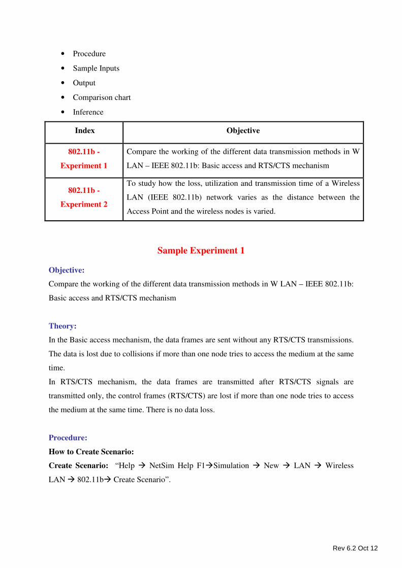
• Procedure
• Sample Inputs
• Output
• Comparison chart
• Inference
Index Objective
802.11b -
Experiment 1
Compare the working of the different data transmission methods in W
LAN – IEEE 802.11b: Basic access and RTS/CTS mechanism
802.11b -
Experiment 2
To study how the loss, utilization and transmission time of a Wireless
LAN (IEEE 802.11b) network varies as the distance between the
Access Point and the wireless nodes is varied.
Sample Experiment 1
Objective:
Compare the working of the different data transmission methods in W LAN – IEEE 802.11b:
Basic access and RTS/CTS mechanism
Theory:
In the Basic access mechanism, the data frames are sent without any RTS/CTS transmissions.
The data is lost due to collisions if more than one node tries to access the medium at the same
time.
In RTS/CTS mechanism, the data frames are transmitted after RTS/CTS signals are
transmitted only, the control frames (RTS/CTS) are lost if more than one node tries to access
the medium at the same time. There is no data loss.
Procedure:
How to Create Scenario:
Create Scenario: “Help � NetSim Help F1�Simulation � New � LAN � Wireless
LAN � 802.11b� Create Scenario”.
Rev 6.2 Oct 12
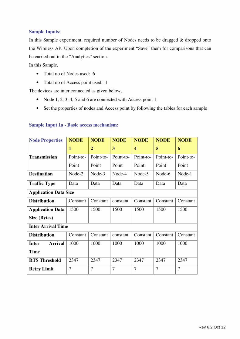
Sample Inputs:
In this Sample experiment, required number of Nodes needs to be dragged & dropped onto
the Wireless AP. Upon completion of the experiment “Save” them for comparisons that can
be carried out in the “Analytics” section.
In this Sample,
• Total no of Nodes used: 6
• Total no of Access point used: 1
The devices are inter connected as given below,
• Node 1, 2, 3, 4, 5 and 6 are connected with Access point 1.
• Set the properties of nodes and Access point by following the tables for each sample
Sample Input 1a - Basic access mechanism:
Node Properties NODE
1
NODE
2
NODE
3
NODE
4
NODE
5
NODE
6
Transmission Point-to-
Point
Point-to-
Point
Point-to-
Point
Point-to-
Point
Point-to-
Point
Point-to-
Point
Destination Node-2 Node-3 Node-4 Node-5 Node-6 Node-1
Traffic Type Data Data Data Data Data Data
Application Data Size
Distribution Constant Constant constant Constant Constant Constant
Application Data
Size (Bytes)
1500 1500 1500 1500 1500 1500
Inter Arrival Time
Distribution Constant Constant constant Constant Constant Constant
Inter Arrival
Time
1000 1000 1000 1000 1000 1000
RTS Threshold 2347 2347 2347 2347 2347 2347
Retry Limit 7 7 7 7 7 7
Rev 6.2 Oct 12
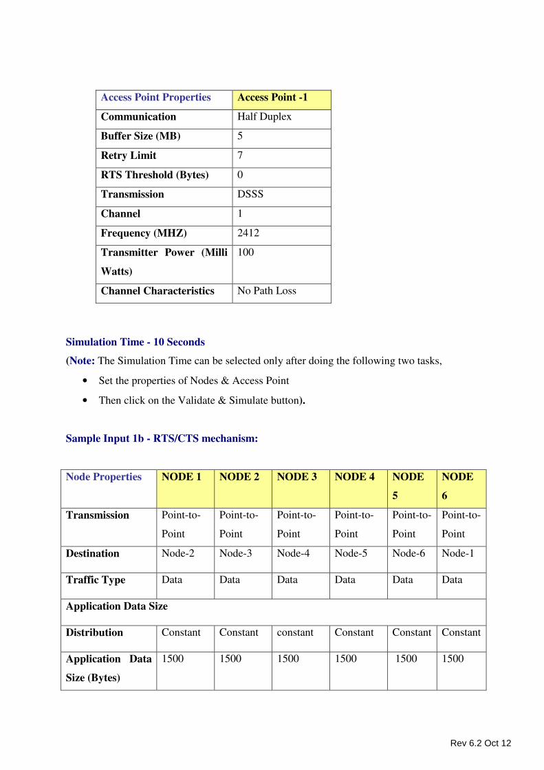
Simulation Time - 10 Seconds
(Note: The Simulation Time can be selected only after doing the following two tasks,
• Set the properties of Nodes & Access Point
• Then click on the Validate & Simulate button).
Sample Input 1b - RTS/CTS mechanism:
Node Properties NODE 1 NODE 2 NODE 3 NODE 4 NODE
5
NODE
6
Transmission Point-to-
Point
Point-to-
Point
Point-to-
Point
Point-to-
Point
Point-to-
Point
Point-to-
Point
Destination Node-2 Node-3 Node-4 Node-5 Node-6 Node-1
Traffic Type Data Data Data Data Data Data
Application Data Size
Distribution Constant Constant constant Constant Constant Constant
Application Data
Size (Bytes)
1500 1500 1500 1500 1500 1500
Access Point Properties Access Point -1
Communication Half Duplex
Buffer Size (MB) 5
Retry Limit 7
RTS Threshold (Bytes) 0
Transmission DSSS
Channel 1
Frequency (MHZ) 2412
Transmitter Power (Milli
Watts)
100
Channel Characteristics No Path Loss
Rev 6.2 Oct 12
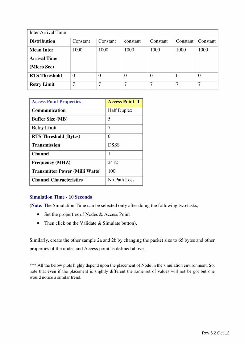
Inter Arrival Time
Distribution Constant Constant constant Constant Constant Constant
Mean Inter
Arrival Time
(Micro Sec)
1000 1000 1000 1000 1000 1000
RTS Threshold 0 0 0 0 0 0
Retry Limit 7 7 7 7 7 7
Access Point Properties Access Point -1
Communication Half Duplex
Buffer Size (MB) 5
Retry Limit 7
RTS Threshold (Bytes) 0
Transmission DSSS
Channel 1
Frequency (MHZ) 2412
Transmitter Power (Milli Watts) 100
Channel Characteristics No Path Loss
Simulation Time - 10 Seconds
(Note: The Simulation Time can be selected only after doing the following two tasks,
• Set the properties of Nodes & Access Point
• Then click on the Validate & Simulate button).
Similarly, create the other sample 2a and 2b by changing the packet size to 65 bytes and other
properties of the nodes and Access point as defined above.
*** All the below plots highly depend upon the placement of Node in the simulation environment. So,
note that even if the placement is slightly different the same set of values will not be got but one
would notice a similar trend.
Rev 6.2 Oct 12
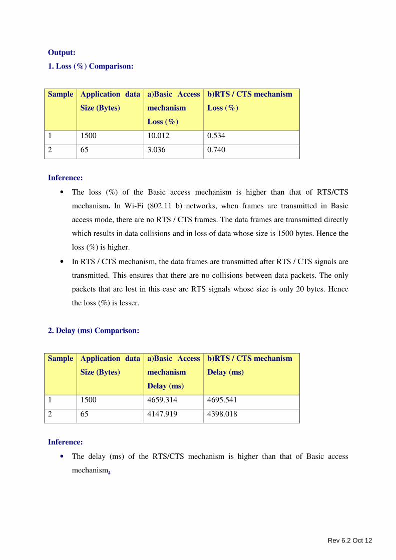
Output:
1. Loss (%) Comparison:
Sample Application data
Size (Bytes)
a)Basic Access
mechanism
Loss (%)
b)RTS / CTS mechanism
Loss (%)
1 1500 10.012 0.534
2 65 3.036 0.740
Inference:
• The loss (%) of the Basic access mechanism is higher than that of RTS/CTS
mechanism. In Wi-Fi (802.11 b) networks, when frames are transmitted in Basic
access mode, there are no RTS / CTS frames. The data frames are transmitted directly
which results in data collisions and in loss of data whose size is 1500 bytes. Hence the
loss (%) is higher.
• In RTS / CTS mechanism, the data frames are transmitted after RTS / CTS signals are
transmitted. This ensures that there are no collisions between data packets. The only
packets that are lost in this case are RTS signals whose size is only 20 bytes. Hence
the loss (%) is lesser.
2. Delay (ms) Comparison:
Sample Application data
Size (Bytes)
a)Basic Access
mechanism
Delay (ms)
b)RTS / CTS mechanism
Delay (ms)
1 1500 4659.314 4695.541
2 65 4147.919 4398.018
Inference:
• The delay (ms) of the RTS/CTS mechanism is higher than that of Basic access
mechanism.
Rev 6.2 Oct 12
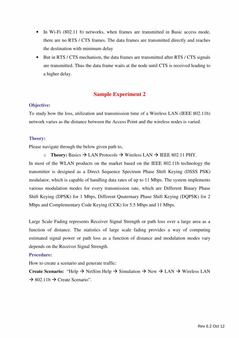
• In Wi-Fi (802.11 b) networks, when frames are transmitted in Basic access mode,
there are no RTS / CTS frames. The data frames are transmitted directly and reaches
the destination with minimum delay
• But in RTS / CTS mechanism, the data frames are transmitted after RTS / CTS signals
are transmitted. Thus the data frame waits at the node until CTS is received leading to
a higher delay.
Sample Experiment 2
Objective:
To study how the loss, utilization and transmission time of a Wireless LAN (IEEE 802.11b)
network varies as the distance between the Access Point and the wireless nodes is varied.
Theory:
Please navigate through the below given path to,
o Theory: Basics � LAN Protocols � Wireless LAN � IEEE 802.11 PHY.
In most of the WLAN products on the market based on the IEEE 802.11b technology the
transmitter is designed as a Direct Sequence Spectrum Phase Shift Keying (DSSS PSK)
modulator, which is capable of handling data rates of up to 11 Mbps. The system implements
various modulation modes for every transmission rate, which are Different Binary Phase
Shift Keying (DPSK) for 1 Mbps, Different Quaternary Phase Shift Keying (DQPSK) for 2
Mbps and Complementary Code Keying (CCK) for 5.5 Mbps and 11 Mbps.
Large Scale Fading represents Receiver Signal Strength or path loss over a large area as a
function of distance. The statistics of large scale fading provides a way of computing
estimated signal power or path loss as a function of distance and modulation modes vary
depends on the Receiver Signal Strength.
Procedure:
How to create a scenario and generate traffic:
Create Scenario: “Help � NetSim Help � Simulation � New � LAN � Wireless LAN
� 802.11b � Create Scenario”.
Rev 6.2 Oct 12
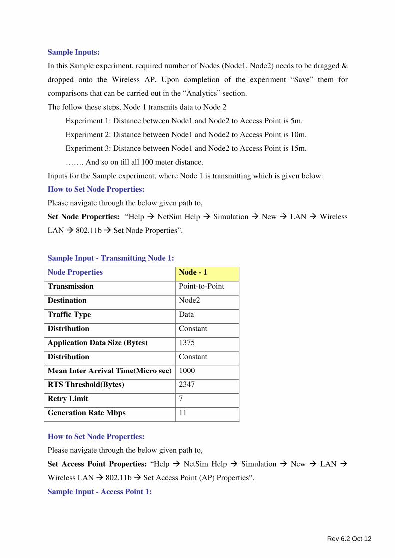
Sample Inputs:
In this Sample experiment, required number of Nodes (Node1, Node2) needs to be dragged &
dropped onto the Wireless AP. Upon completion of the experiment “Save” them for
comparisons that can be carried out in the “Analytics” section.
The follow these steps, Node 1 transmits data to Node 2
Experiment 1: Distance between Node1 and Node2 to Access Point is 5m.
Experiment 2: Distance between Node1 and Node2 to Access Point is 10m.
Experiment 3: Distance between Node1 and Node2 to Access Point is 15m.
……. And so on till all 100 meter distance.
Inputs for the Sample experiment, where Node 1 is transmitting which is given below:
How to Set Node Properties:
Please navigate through the below given path to,
Set Node Properties: “Help � NetSim Help � Simulation � New � LAN � Wireless
LAN � 802.11b � Set Node Properties”.
Sample Input - Transmitting Node 1:
How to Set Node Properties:
Please navigate through the below given path to,
Set Access Point Properties: “Help � NetSim Help � Simulation � New � LAN �
Wireless LAN � 802.11b � Set Access Point (AP) Properties”.
Sample Input - Access Point 1:
Node Properties Node - 1
Transmission Point-to-Point
Destination Node2
Traffic Type Data
Distribution Constant
Application Data Size (Bytes) 1375
Distribution Constant
Mean Inter Arrival Time(Micro sec) 1000
RTS Threshold(Bytes) 2347
Retry Limit 7
Generation Rate Mbps 11
Rev 6.2 Oct 12
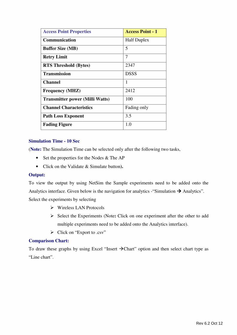
Access Point Properties Access Point - 1
Communication Half Duplex
Buffer Size (MB) 5
Retry Limit 7
RTS Threshold (Bytes) 2347
Transmission DSSS
Channel 1
Frequency (MHZ) 2412
Transmitter power (Milli Watts) 100
Channel Characteristics Fading only
Path Loss Exponent 3.5
Fading Figure 1.0
Simulation Time - 10 Sec
(Note: The Simulation Time can be selected only after the following two tasks,
• Set the properties for the Nodes & The AP
• Click on the Validate & Simulate button).
Output:
To view the output by using NetSim the Sample experiments need to be added onto the
Analytics interface. Given below is the navigation for analytics -“Simulation ���� Analytics”.
Select the experiments by selecting
� Wireless LAN Protocols
� Select the Experiments (Note: Click on one experiment after the other to add
multiple experiments need to be added onto the Analytics interface).
� Click on “Export to .csv”
Comparison Chart:
To draw these graphs by using Excel “Insert �Chart” option and then select chart type as
“Line chart”.
Rev 6.2 Oct 12
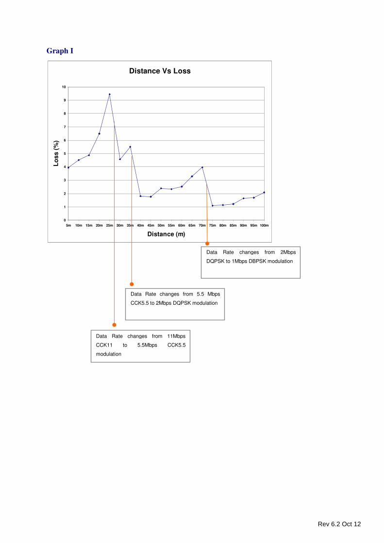
Graph I
Distance Vs Loss
0
1
2
3
4
5
6
7
8
9
10
5m 10m 15m 20m 25m 30m 35m 40m 45m 50m 55m 60m 65m 70m 75m 80m 85m 90m 95m 100m
Distance (m)
Lo
ss
(%
)
Data Rate changes from 11Mbps
CCK11 to 5.5Mbps CCK5.5
modulation
Data Rate changes from 5.5 Mbps
CCK5.5 to 2Mbps DQPSK modulation
Data Rate changes from 2Mbps
DQPSK to 1Mbps DBPSK modulation
Rev 6.2 Oct 12
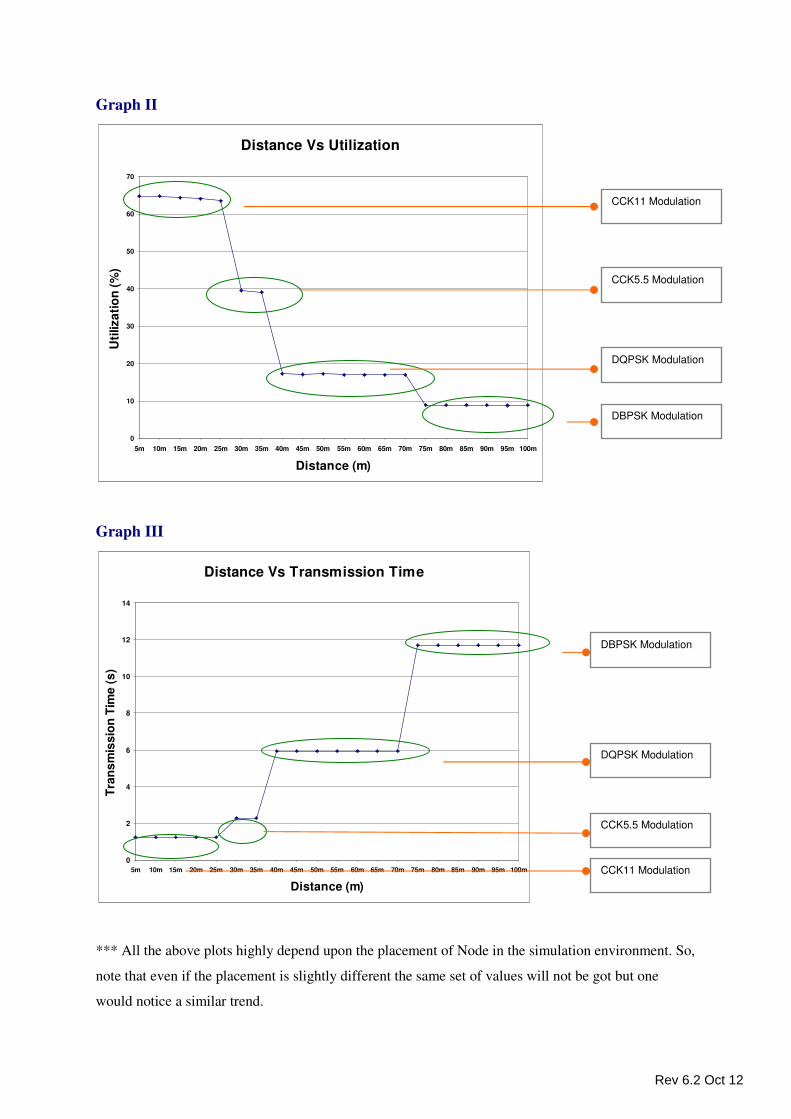
Graph II
Distance Vs Utilization
0
10
20
30
40
50
60
70
5m 10m 15m 20m 25m 30m 35m 40m 45m 50m 55m 60m 65m 70m 75m 80m 85m 90m 95m 100m
Distance (m)
Uti
liza
tio
n (
%)
Graph III
Distance Vs Transmission Time
0
2
4
6
8
10
12
14
5m 10m 15m 20m 25m 30m 35m 40m 45m 50m 55m 60m 65m 70m 75m 80m 85m 90m 95m 100m
Distance (m)
Tra
ns
mis
sio
n T
ime
(s
)
*** All the above plots highly depend upon the placement of Node in the simulation environment. So,
note that even if the placement is slightly different the same set of values will not be got but one
would notice a similar trend.
CCK11 Modulation
CCK5.5 Modulation
DQPSK Modulation
DBPSK Modulation
CCK11 Modulation
CCK5.5 Modulation
DQPSK Modulation
DBPSK Modulation
Rev 6.2 Oct 12
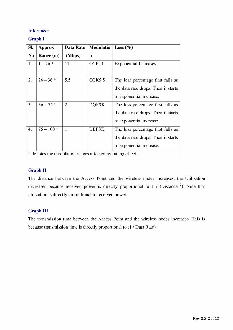
Inference:
Graph I
Sl.
No
Approx
Range (m)
Data Rate
(Mbps)
Modulatio
n
Loss (%)
1. 1 – 26 * 11 CCK11 Exponential Increases.
2. 26 – 36 * 5.5 CCK5.5 The loss percentage first falls as
the data rate drops. Then it starts
to exponential increase.
3. 36 - 75 * 2 DQPSK The loss percentage first falls as
the data rate drops. Then it starts
to exponential increase.
4. 75 – 100 * 1 DBPSK The loss percentage first falls as
the data rate drops. Then it starts
to exponential increase.
* denotes the modulation ranges affected by fading effect.
Graph II
The distance between the Access Point and the wireless nodes increases, the Utilization
decreases because received power is directly proportional to 1 / (Distance 2). Note that
utilization is directly proportional to received power.
Graph III
The transmission time between the Access Point and the wireless nodes increases. This is
because transmission time is directly proportional to (1 / Data Rate).
Rev 6.2 Oct 12
Wireless LAN - 802.11g
New Experiments
In the Simulation menu select � New � LAN � Ethernet � Wireless LAN ���� 802.11g.
To perform experiments in Wireless LAN, the following steps should be followed,
• Create Scenario
• Set Node Properties
• Set Access Point (AP) Properties
• Remove Devices (or) Links
• Simulate
Create Scenario
Adding Wireless AP - Click on the Wireless AP icon and drag it onto the environment
builder.
Adding Switch - Click on the Switch icon and drag it onto the environment builder. By
default a Switch consists of eight ports.
Adding Node -
• Click on the Node icon and drag and drop it on the Wireless AP.
• Nodes cannot be connected directly to each other because an intermediate
connecting component (such as Switch) is required.
• A Node cannot be placed on another Node. It has to be dragged and placed on any
connecting component.
Establishing Connections between Switch, Wireless AP and Nodes - Click the two
devices to connect them. These two devices are connected via a Link.
Set Node Properties
Right Click on the appropriate node to select Properties. Inside the properties’ window click
on Application 1 to modify its properties.
Transmission Type
This indicates the type of transmission made by this session, either Broadcast or Point to
Point.
Destination
This property indicates the Destination Node.
Rev 6.2 Oct 12
Traffic Type
This property indicates the type of traffic. The traffic can either be Voice or Data.
Voice
Codec
Codec is the component of any voice system that translates between analog speech and
the bits used to transmit them. Every codec transmits a burst of data in a packet that can
be reconstructed into voice. Five different standards of voice codec’s are given which
can be selected depending on the variations required.
Service Type
• CBR - CBR stands for Constant Bit Rate. Packets of constant size are generated at
constant inter arrival times.
• VBR - VBR stands for Variable Bit Rate. The two types of Suppression Model
that can be selected are,
• Deterministic
• Markov Chain
Click OK to accept the user entered values. Click on the close button at the top right
corner to exit the screen.
Data
Packet Size
Distribution: The options available for distribution are,
• Constant
• Exponential
Mean Packet Size (Bytes): Sets the size of the packets being generated by the chosen
distribution. The range of values that can be entered are between 65 to 1500 bytes. By
default 1500 bytes is entered.
Inter Arrival Time
This indicates the time gap between packets.
Distribution : The options available for distribution are,
• Constant
• Exponential
• Uniform
Mean Inter Arrival Time: Enter the average inter-arrival time between packets. A
lower inter-arrival time would lead to a higher generation rate and the vice versa. The
range of values that can be entered are between 1000 to 20000 Micro Sec. By default
20000 Micro Sec is entered.
Click OK to accept the user entered values. Click on the close button at the top right
corner to exit the screen.
Rev 6.2 Oct 12
RTS Threshold (Bytes)
This is to allow the node to enable/disable the RTS/CTS mechanism. The valid value
ranges from “0 to 2347”. Default values is 0 bytes.
Retry Limit
This indicates the number of attempts that can be made by a frame. The option varies
from 1 to 7.
Modifying/Viewing/Accepting Properties
On opening an already configured properties of an application the input fields will be
frozen (i.e. the input cannot be changed).To modify these values click on the Modify
button in the screen. Now the input value can be changed. Click on the Accept button,
the modified values will be saved.
This View button is enabled once the Accept Button is clicked. To view the given
values, click on the View button.
Set Access Point (AP) Properties
Right click on the appropriate Access Point (AP) and click Properties. Options available
are,
Wireless Properties - Under Wireless Properties tab the options available are,
Connected To - This property defines the Wireless Medium connected to the Access
Point (AP). A default value is already entered; hence no changes can be done.
Communication - This property defines the Communication mode of the network. By
default, a Wireless LAN network works in Half Duplex. This property cannot be
changed.
Data Link Layer - Under Data Link Layer the sub-options available are,
MAC Address - A default value has been coded in, hence no change can be made.
Buffer Size (MB) - This property defines the buffer capacity of the Wireless Port.
Options available are � “1, 2, 3, 4 and 5”. Default value is 5MB.
Retry Limit - Indicate the number of attempts that can be made by a frame. This varies
from 1 to 7. By default the Retry Limit value is 7.
RTS Threshold (Bytes) - This property is to allow the node to enable/disable the
RTS/CTS mechanism. By default the value that is available is 0 Bytes. Limit ranges
from 0 to 2347 Bytes.
Physical Layer - Under Physical Layer the sub-options available are,
Standard - This property gives the standard that is followed for modeling Physical
Layer. By default the standard is IEEE 802.11g can be found next to this property.
Rev 6.2 Oct 12
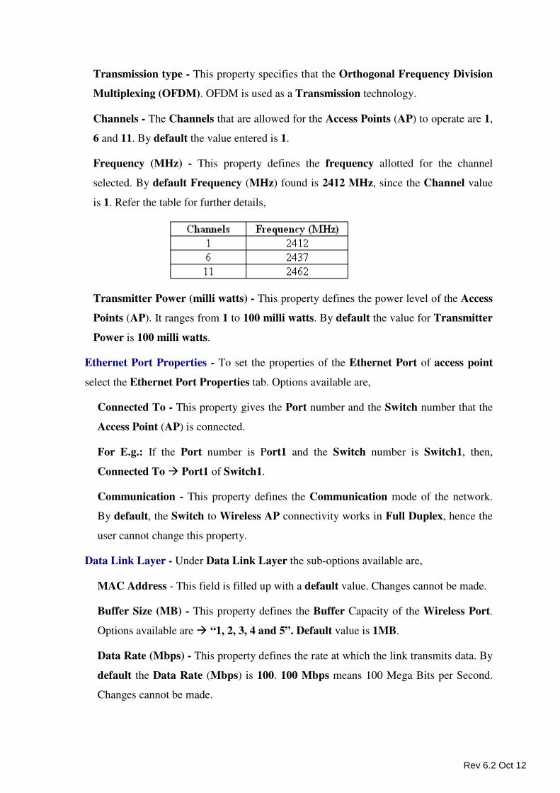
Transmission type - This property specifies that the Orthogonal Frequency Division
Multiplexing (OFDM). OFDM is used as a Transmission technology.
Channels - The Channels that are allowed for the Access Points (AP) to operate are 1,
6 and 11. By default the value entered is 1.
Frequency (MHz) - This property defines the frequency allotted for the channel
selected. By default Frequency (MHz) found is 2412 MHz, since the Channel value
is 1. Refer the table for further details,
Transmitter Power (milli watts) - This property defines the power level of the Access
Points (AP). It ranges from 1 to 100 milli watts. By default the value for Transmitter
Power is 100 milli watts.
Ethernet Port Properties - To set the properties of the Ethernet Port of access point
select the Ethernet Port Properties tab. Options available are,
Connected To - This property gives the Port number and the Switch number that the
Access Point (AP) is connected.
For E.g.: If the Port number is Port1 and the Switch number is Switch1, then,
Connected To � Port1 of Switch1.
Communication - This property defines the Communication mode of the network.
By default, the Switch to Wireless AP connectivity works in Full Duplex, hence the
user cannot change this property.
Data Link Layer - Under Data Link Layer the sub-options available are,
MAC Address - This field is filled up with a default value. Changes cannot be made.
Buffer Size (MB) - This property defines the Buffer Capacity of the Wireless Port.
Options available are � “1, 2, 3, 4 and 5”. Default value is 1MB.
Data Rate (Mbps) - This property defines the rate at which the link transmits data. By
default the Data Rate (Mbps) is 100. 100 Mbps means 100 Mega Bits per Second.
Changes cannot be made.
Rev 6.2 Oct 12
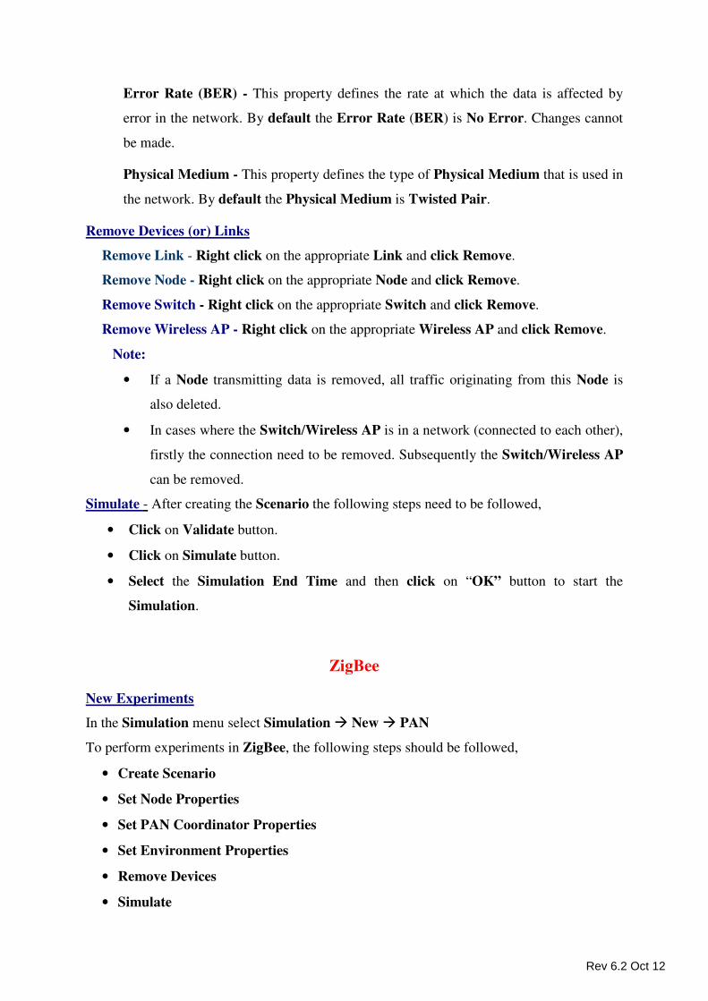
Error Rate (BER) - This property defines the rate at which the data is affected by
error in the network. By default the Error Rate (BER) is No Error. Changes cannot
be made.
Physical Medium - This property defines the type of Physical Medium that is used in
the network. By default the Physical Medium is Twisted Pair.
Remove Devices (or) Links
Remove Link - Right click on the appropriate Link and click Remove.
Remove Node - Right click on the appropriate Node and click Remove.
Remove Switch - Right click on the appropriate Switch and click Remove.
Remove Wireless AP - Right click on the appropriate Wireless AP and click Remove.
Note:
• If a Node transmitting data is removed, all traffic originating from this Node is
also deleted.
• In cases where the Switch/Wireless AP is in a network (connected to each other),
firstly the connection need to be removed. Subsequently the Switch/Wireless AP
can be removed.
Simulate - After creating the Scenario the following steps need to be followed,
• Click on Validate button.
• Click on Simulate button.
• Select the Simulation End Time and then click on “OK” button to start the
Simulation.
ZigBee
New Experiments
In the Simulation menu select Simulation � New � PAN
To perform experiments in ZigBee, the following steps should be followed,
• Create Scenario
• Set Node Properties
• Set PAN Coordinator Properties
• Set Environment Properties
• Remove Devices
• Simulate
Rev 6.2 Oct 12
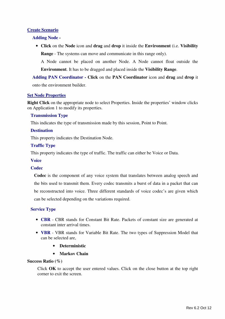
Create Scenario
Adding Node -
• Click on the Node icon and drag and drop it inside the Environment (i.e. Visibility
Range - The systems can move and communicate in this range only).
A Node cannot be placed on another Node. A Node cannot float outside the
Environment. It has to be dragged and placed inside the Visibility Range.
Adding PAN Coordinator - Click on the PAN Coordinator icon and drag and drop it
onto the environment builder.
Set Node Properties
Right Click on the appropriate node to select Properties. Inside the properties’ window clicks
on Application 1 to modify its properties.
Transmission Type
This indicates the type of transmission made by this session, Point to Point.
Destination
This property indicates the Destination Node.
Traffic Type
This property indicates the type of traffic. The traffic can either be Voice or Data.
Voice
Codec
Codec is the component of any voice system that translates between analog speech and
the bits used to transmit them. Every codec transmits a burst of data in a packet that can
be reconstructed into voice. Three different standards of voice codec’s are given which
can be selected depending on the variations required.
Service Type
• CBR - CBR stands for Constant Bit Rate. Packets of constant size are generated at
constant inter arrival times.
• VBR - VBR stands for Variable Bit Rate. The two types of Suppression Model that
can be selected are,
• Deterministic
• Markov Chain
Success Ratio (%)
Click OK to accept the user entered values. Click on the close button at the top right
corner to exit the screen.
Rev 6.2 Oct 12
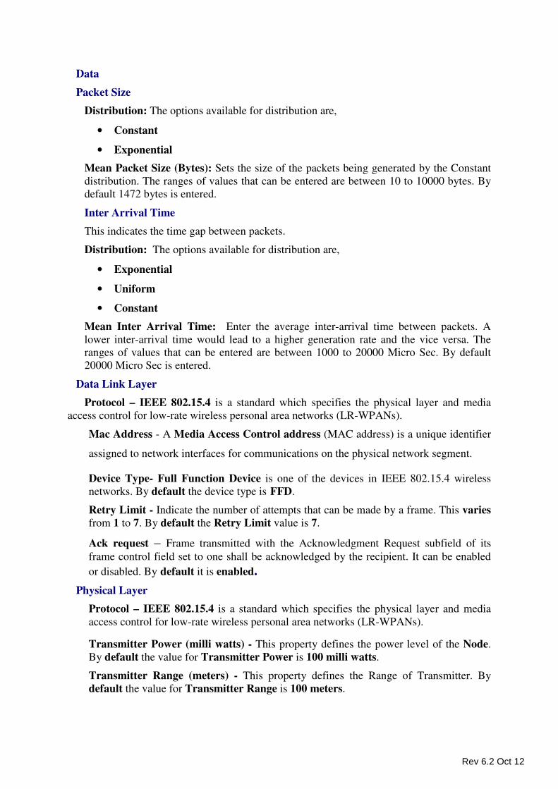
Data
Packet Size
Distribution: The options available for distribution are,
• Constant
• Exponential
Mean Packet Size (Bytes): Sets the size of the packets being generated by the Constant
distribution. The ranges of values that can be entered are between 10 to 10000 bytes. By
default 1472 bytes is entered.
Inter Arrival Time
This indicates the time gap between packets.
Distribution: The options available for distribution are,
• Exponential
• Uniform
• Constant
Mean Inter Arrival Time: Enter the average inter-arrival time between packets. A
lower inter-arrival time would lead to a higher generation rate and the vice versa. The
ranges of values that can be entered are between 1000 to 20000 Micro Sec. By default
20000 Micro Sec is entered.
Data Link Layer
Protocol – IEEE 802.15.4 is a standard which specifies the physical layer and media
access control for low-rate wireless personal area networks (LR-WPANs).
Mac Address - A Media Access Control address (MAC address) is a unique identifier
assigned to network interfaces for communications on the physical network segment.
Device Type- Full Function Device is one of the devices in IEEE 802.15.4 wireless
networks. By default the device type is FFD.
Retry Limit - Indicate the number of attempts that can be made by a frame. This varies
from 1 to 7. By default the Retry Limit value is 7.
Ack request – Frame transmitted with the Acknowledgment Request subfield of its
frame control field set to one shall be acknowledged by the recipient. It can be enabled
or disabled. By default it is enabled.
Physical Layer
Protocol – IEEE 802.15.4 is a standard which specifies the physical layer and media
access control for low-rate wireless personal area networks (LR-WPANs).
Transmitter Power (milli watts) - This property defines the power level of the Node.
By default the value for Transmitter Power is 100 milli watts.
Transmitter Range (meters) - This property defines the Range of Transmitter. By
default the value for Transmitter Range is 100 meters.
Rev 6.2 Oct 12
This View button is enabled once the Accept Button is clicked. To view the given
values, click on the View button.
Click OK to accept the user entered values. Click on the close button at the top right
corner to exit the screen.
Modifying/Viewing/Accepting Properties
On opening an already configured properties of an application the input fields will be
frozen (i.e. the input cannot be changed).To modify these values click on the Modify
button in the screen. Now the input value can be changed. Click on the Accept button,
the modified values will be saved.
This View button is enabled once the Accept Button is clicked. To view the given
values, click on the View button.
Set PAN Coordinator Properties
Right Click on the PAN Coordinator and click Properties. Options available are,
PAN Coordinator Properties
Data Link Layer - The options available under this property is,
Protocol – IEEE 802.15.4 is a standard which specifies the physical layer and media
access control for low-rate wireless personal area networks (LR-WPANs).
Beacon Mode – Beacon Mode defines synchronization and reliability of the transmission
mechanism, whereas beaconless networks adopt a simple lightweight protocol based on
CSMA-CA. There are two options available, Enable/Disable. Default is set as enable
Beacon Order – Beacon Order, describes the interval at which the coordinator shall
transmit its beacon frames. 15 denotes that beacon mode is disabled, if Beacon mode is
enabled then the Beacon Order value can range from 0 to 14. Default Beacon Order
value is 15.
Superframe Order – Superframe Order describes the length of the active portion of the
superframe, which includes the beacon frame. This property will be there, only in case of
beacon mode is enabled. The value of Superframe Order should be less than 15. Default
value is 15.
Rev 6.2 Oct 12

GTS Mode - GTS (Guaranteed Time Slot) allows a device to operate on the channel
within a portion of the superframe that is dedicated (on the PAN) exclusively to that
device. This property will be there, only if beacon mode is enabled. By default the GTS
Mode is enabled.
Superframe Duration – The Superframe Duration (SD) is divided into 16 equally sized
time slots, during which data transmission is allowed. The SD can be further divided into
a Contention Access Period (CAP)and an optional Contention Free Period (CFP)
composed of Guaranteed Time Slots. A default value has been coded in; hence no change
can be made. The fixed value is 15.36 ms.
Battery Life Extension – The Battery Life Extension (BLE) subfield is 1 bit in length
and shall be set to one if frames transmitted to the beaconing device during its
CAP(Contention Access Period) are required to start on or before macBattLifeExtPeriods
full backoff periods after the IFS (inter frame space or spacing) period following the
beacon. Otherwise, the BLE subfield shall be set to 0. The options available are
True/False. This property will be there, only in case of beacon mode is enabled. By
default the Battery Life Extension mode is true.
Maximum Backoff Exponent – The maximum value of the backoff exponent (BE) in
the CSMA-CA algorithm. The Maximum Backoff Exponent value ranges from 3 to 8.
Default value is 5.
Minimum Backoff Exponent – The minimum value of the backoff exponent (BE) in the
CSMA-CA algorithm. The Minimum Backoff Exponent value rangse from 0 to Max BE.
Default value is 5.
Max Frame retries – The maximum number of retries allowed after a transmission
failure. The Max Frame retries value ranges from 0 to 7. By default the Max Frame
retries value is 3.
MAX CSMA Backoff - The maximum number of backoffs the CSMA-CA algorithm
will attempt before declaring a channel access failure. The MAX CSMA Backoff value
ranges from 0 to 5. Default value is 4.
Rev 6.2 Oct 12
Unit Backoff Period - The number of symbols forming the basic time period used by the
CSMA-CA algorithm. A default value has been coded in; hence no change can be made.
The value is 20 Symbols.
Min CAP length - The minimum number of symbols forming the CAP (contention
access period).This ensures that MAC commands can still be transferred to devices when
GTSs (Guaranteed Time Slot) are being used. A default value has been coded in; hence
no change can be made. The value is 440 Symbols
GTS descriptor Persistent Time - A default value has been coded in; hence no change
can be made. The GTS descriptor Persistent Time is 4 s.
Physical Layer - The options available under this property is,
Protocol – IEEE 802.15.4 Phy - IEEE 802.15.4 is a standard which specifies the
physical layer and media access control for low-rate wireless personal area networks (LR-
WPANs).
Frequency Band - Frequency bands are groupings of radio frequencies that are used by
mobile networks to communicate with mobile phones. A default value has been coded in;
hence no change can be made. The value is 2.4 GHz.
Data Rate - Data rate or bit rate is the number of bits that are conveyed or processed per
unit of time. A default value has been coded in; hence no change can be made. The value
is 250 kbps.
Chip Rate - The chip rate of a code is the number of pulses per second (chips per second)
at which the code is transmitted (or received). The chip rate is larger than the symbol rate,
meaning that one symbol is represented by multiple chips. A default value has been
coded in; hence no change can be made. The value is 2000 McPs.
Symbol Rate - In digital communications, symbol rate (also known as baud or
modulation rate) is the number of symbol changes (waveform changes or signaling
events) made to the transmission medium per second using a digitally modulated signal or
a line code. A default value has been coded in; hence no change can be made. The value
is 62.5 KSymbolsPS.
Rev 6.2 Oct 12
Modulation Technique - Offset quadrature phase-shift keying (OQPSK) is a variant of
phase-shift keying modulation using 4 different values of the phase to transmit. It is
sometimes called staggered quadrature phase-shift keying (SQPSK).
Min LIFS period - The minimum number of symbols forming a LIFS (Long Inter Frame
Spacing) period. A default value has been coded in; hence no change can be made. The
value is 40 Symbols.
Min SIFS period - The minimum number of symbols forming a SIFS (Short Inter Frame
Spacing) period. A default value has been coded in; hence no change can be made. The
value is 20 Symbols.
Unit Backoff Time - The number of symbols forming the basic time period used by the
CSMA-CA algorithm. A default value has been coded in; hence no change can be made.
The value is 20 Symbols.
Turn Around Time - The TX-to-RX turnaround time is defined as the shortest time
possible at the air interface from the trailing edge of the last chip (of the last symbol) of a
transmitted PPDU to the leading edge of the first chip (of the first symbol) of the next
received PPDU. The RX-to-TX turnaround time is defined as the shortest time possible at
the air interface from the trailing edge of the last chip (of the last symbol) of a received
PPDU to the leading edge of the first chip (of the first symbol) of the next transmitted
PPDU. A default value has been coded in; hence no change can be made. The value is 12
Symbols.
Phy SHR Duration – The duration of the synchronization header (SHR) in symbols for
the current PHY. The Values available are 3, 7, 10, and 40. By default Phy SHR
Duration is 3.
Phy Symbol Per Octet - The number of symbols per octet for the current PHY. The
Values available are 0.4, 1.6, 2, 8. By default phy symbol per octet is 0.4.
CCA mode
The following are the available options under CCA mode,
• Carrier Sense Only (by default this options is selected).
CCA (Clear Channel Assessment) shall report a busy medium only upon the
detection of a signal compliant with this standard with the same modulation and
Rev 6.2 Oct 12
spreading characteristics of the PHY that is currently in use by the device. This
signal may be above or below the ED threshold.
• Energy Detection
CCA shall report a busy medium upon detecting any energy above the ED
threshold.
• Carrier Sense with Energy Detection
CCA shall report a busy medium using a logical combination of Detection of a
signal with the modulation and spreading characteristics of this standard and
Energy above the ED threshold, where the logical operator may be AND/OR.
Receiver Sensitivity –Threshold input signal power that yields a specified PER (packet
error rate) conditions PSDU (PHY service data unit) length = 20 octets PER less than 1%
Power measured at antenna terminals. Interference not present The Receiver Sensitivity
Value should be less than 0. Default value is -85 dbm.
ED threshold - The receiver ED threshold is intended for use by a network layer as part
of a channel selection algorithm. It is an estimate of the received signal power within the
bandwidth of the channel. No attempt is made to identify or decode signals on the
channel. If the receive signal power is greater than the ED threshold value then the
channel selection algorithm will return false. The ED threshold Value should be less
than 0. Default value is -95 dbm.
Set Environment Properties
Right click in side of the on the Environment and click Properties.
Channels - There are sixteen non-overlapping channel numbered from 11 to 26 for 2450
MHz band in 802.15.4 standard. Default value is 11.
Frequency (MHz) - This property defines the frequency allotted for the channel selected.
By default Frequency (MHz) used is 2405 MHz, since the Channel value is 11.
Channel Characteristics - This property defines the Channel Characteristics for the
Agent. It consists of the following options.
• Fading and Shadowing (default option).
• Fading only
• Line of Sight
Rev 6.2 Oct 12
• No Path Loss
Path loss Exponent – Path loss exponent indicates the rate at which the path loss
increases with distance. The value depends on the specific propagation environment. The
value varies range from 2 to 5. The default value is 3.5. This property will be enabled only
for Fading and Shadowing, Fading only, and Line of Sight.
Fading Figure m (0.5 to 5) - The parameter ‘m’, the “fading figure”, is defined as the
ratio of moments, and the default value is 1.0. The value of m = 1 corresponds to Rayleigh
fading, and m > 1 indicates better fading conditions than Rayleigh and usually indicates
Line of Sight available between agent. This value varies from 0.5 to 5. This property will
be enabled only for Fading and Shadowing, and Fading only.
Standard Deviation - Shadowing is caused mainly by terrain features of the radio
propagation environment. The mathematical model for shadowing is a log-normal
distribution with standard deviation of 5 to 12 dB. This has been found to be the best
available data to be taken. The default value is 12 db. This property will be enabled only
for Fading and Shadowing.
Remove Devices (or) Links
Remove Node - Right click on the appropriate Node and click Remove.
Remove PAN Coordinator - Right click on the appropriate PAN Coordinator and click
Remove.
Simulate - After creating the Scenario the following steps need to be followed,
• Click on Validate button.
• Click on Simulate button.
• Select the Simulation End Time and then click on “OK” button to start the
Simulation.
NetSim - ZigBee
Sample Experiments - User can understand the working of ZigBee through these sample
experiments. Each sample experiment covers:
• Procedure
• Sample Inputs
• Output
Rev 6.2 Oct 12
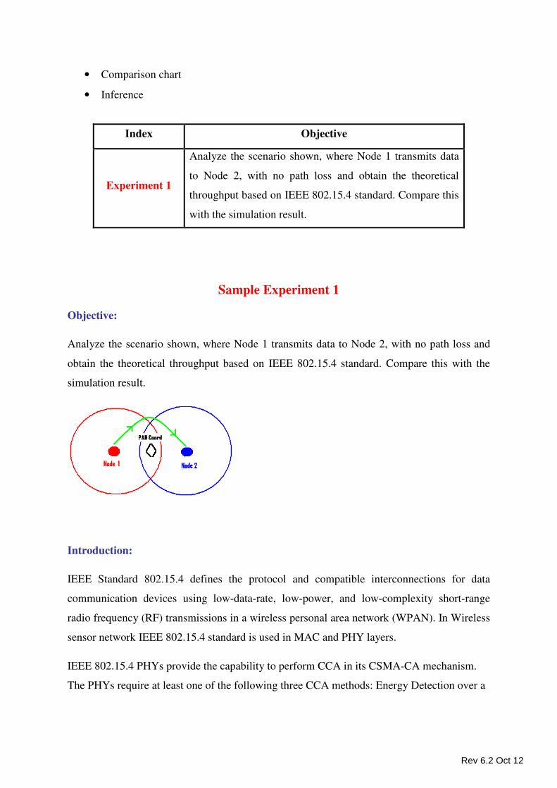
• Comparison chart
• Inference
Index Objective
Experiment 1
Analyze the scenario shown, where Node 1 transmits data
to Node 2, with no path loss and obtain the theoretical
throughput based on IEEE 802.15.4 standard. Compare this
with the simulation result.
Sample Experiment 1
Objective:
Analyze the scenario shown, where Node 1 transmits data to Node 2, with no path loss and
obtain the theoretical throughput based on IEEE 802.15.4 standard. Compare this with the
simulation result.
Introduction:
IEEE Standard 802.15.4 defines the protocol and compatible interconnections for data
communication devices using low-data-rate, low-power, and low-complexity short-range
radio frequency (RF) transmissions in a wireless personal area network (WPAN). In Wireless
sensor network IEEE 802.15.4 standard is used in MAC and PHY layers.
IEEE 802.15.4 PHYs provide the capability to perform CCA in its CSMA-CA mechanism.
The PHYs require at least one of the following three CCA methods: Energy Detection over a
Rev 6.2 Oct 12
certain threshold, detection of a signal with IEEE 802.15.4 characteristics, or a combination
of these methods.
Theory:
• A packet transmission begins with a random backoff (in number of slots, each slot of 20
duration) which is sampled uniformly from 0 to followed by a CCA.
• A CCA failure starts a new backoff process with the backoff exponent raised by one, i.e.,
to macminBE+1, provided it is lesser than the maximum backoff value given by
macmaxBE.
• Maximum number of successive CCA failures for the same packet is governed by
macMaxCSMABackoffs, exceeding which the packet is discarded at the MAC layer.
• A successful CCA is followed by the radio turnaround time and packet transmission.
• If the receiver successfully receives the packet i.e., without any collision or corruption
due to PHY layer noise, the receiver sends an ACK after the radio turnaround time.
• A failed packet reception causes no ACK generation.
• The transmitter infers that the packet has failed after waiting for macAckWaitDuration
and retransmits the packet for a maximum of aMaxFrameRetries times before discarding
it at the MAC layer.
Note:
In NetSim the radio turnaround time after a CCA success is not considered.
Simulation:
How to Create Scenario:
Please navigate through the below given path for Create Scenario Help
“Help � NetSim Help F1�Simulation � New � PAN � ZigBee � Create
Scenario”.
Rev 6.2 Oct 12
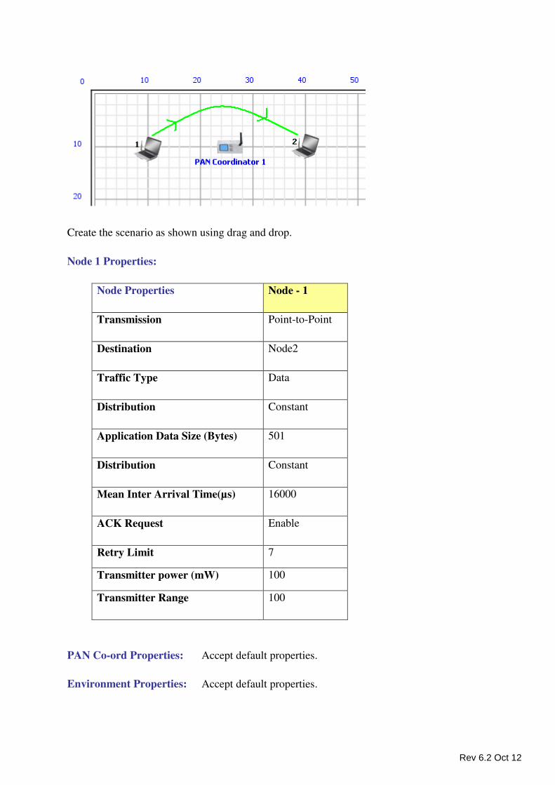
Create the scenario as shown using drag and drop.
Node 1 Properties:
Node Properties Node - 1
Transmission Point-to-Point
Destination Node2
Traffic Type Data
Distribution Constant
Application Data Size (Bytes) 501
Distribution Constant
Mean Inter Arrival Time(µs) 16000
ACK Request Enable
Retry Limit 7
Transmitter power (mW) 100
Transmitter Range 100
PAN Co-ord Properties: Accept default properties.
Environment Properties: Accept default properties.
Rev 6.2 Oct 12
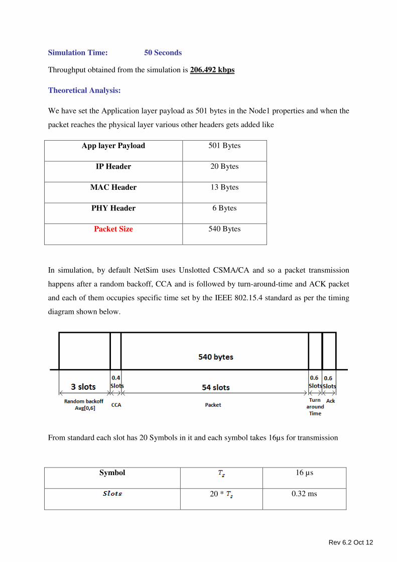
Simulation Time: 50 Seconds
Throughput obtained from the simulation is 206.492 kbps
Theoretical Analysis:
We have set the Application layer payload as 501 bytes in the Node1 properties and when the
packet reaches the physical layer various other headers gets added like
App layer Payload 501 Bytes
IP Header 20 Bytes
MAC Header 13 Bytes
PHY Header 6 Bytes
Packet Size 540 Bytes
In simulation, by default NetSim uses Unslotted CSMA/CA and so a packet transmission
happens after a random backoff, CCA and is followed by turn-around-time and ACK packet
and each of them occupies specific time set by the IEEE 802.15.4 standard as per the timing
diagram shown below.
From standard each slot has 20 Symbols in it and each symbol takes 16µs for transmission
Symbol 16 µs
20 * 0.32 ms
Rev 6.2 Oct 12
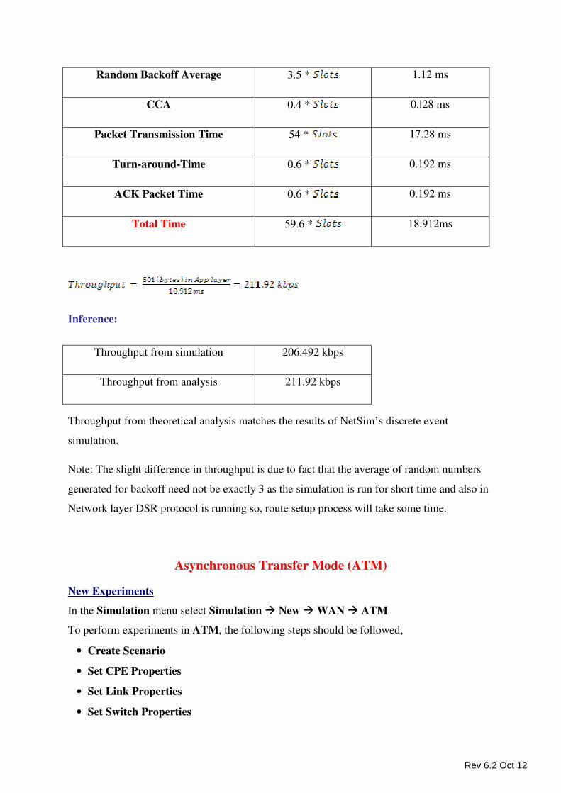
Random Backoff Average 3.5 * 1.12 ms
CCA 0.4 * 0.l28 ms
Packet Transmission Time 54 * 17.28 ms
Turn-around-Time 0.6 * 0.192 ms
ACK Packet Time 0.6 * 0.192 ms
Total Time 59.6 * 18.912ms
Inference:
Throughput from theoretical analysis matches the results of NetSim’s discrete event
simulation.
Note: The slight difference in throughput is due to fact that the average of random numbers
generated for backoff need not be exactly 3 as the simulation is run for short time and also in
Network layer DSR protocol is running so, route setup process will take some time.
Asynchronous Transfer Mode (ATM)
New Experiments
In the Simulation menu select Simulation � New � WAN � ATM
To perform experiments in ATM, the following steps should be followed,
• Create Scenario
• Set CPE Properties
• Set Link Properties
• Set Switch Properties
Throughput from simulation 206.492 kbps
Throughput from analysis 211.92 kbps
Rev 6.2 Oct 12
• Remove Devices (or) Links
• Simulate
Create Scenario
Adding CPE (Customer Premise Equipment) - Click on the CPE icon, drag and drop the
CPE on the environment builder.
Adding ATM Switch - Click on the Switch icon, drag and drop the Switch on the
environment builder. By default a Switch has eight ports.
Establishing Connections between CPE and ATM Switch - The steps for to be followed
are as follows,
• The connections between the two CPEs cannot be made in the network.
• On clicking the two devices connection can be made.
• The connection possibilities are,
o CPE to Switch and
o Switch to Switch.
Set CPE (Customer Premises Equipment) Properties
Right Click on the appropriate node to select Properties. Inside the properties’ window click
on Application 1 to modify its properties.
Transmission Type
This indicates the type of transmission made by this session, only Point to Point
Transmission can be made.
Destination
This property indicates the Destination CPE.
Traffic Type
This property indicates the type of traffic. The traffic can either be Voice or Data.
Voice
Codec
Codec is the component of any voice system that translates between analog speech and
the bits used to transmit them. Every codec transmits a burst of data in a packet that can
be reconstructed into voice. Five different standards of voice codec’s are given which
can be selected depending on the variations required.
Rev 6.2 Oct 12
Service Type
• CBR - CBR stands for Constant Bit Rate. Packets of constant size are generated at
constant inter arrival times.
• VBR - VBR stands for Variable Bit Rate. The two types of Suppression Model that
can be selected are,
• Deterministic
• Markov Chain
Click OK to accept the user entered values. Click on the close button at the top right
corner to exit the screen.
Data
Packet Size
Distribution: The options available for distribution are,
• Constant
• Exponential
Mean Packet Size (Bytes): Sets the size of the packets being generated by the chosen
distribution. The range of values that can be entered are between 65 to 1500 bytes. By
default 1500 bytes is entered.
Inter Arrival Time
This indicates the time gap between packets.
Distribution : The options available for distribution are,
• Constant
• Exponential
• Uniform
Mean Inter Arrival Time: Enter the average inter-arrival time between packets. A
lower inter-arrival time would lead to a higher generation rate and the vice versa. The
range of values that can be entered are between 1000 to 20000 Micro Sec. By default
20000 Micro Sec is entered.
Click OK to accept the user entered values. Click on the close button at the top right
corner to exit the screen.
Data Link Layer
Scheduling: This option consists of
• Round Robin (by default this schedule is set)
• Priority
• FIFO
Rev 6.2 Oct 12
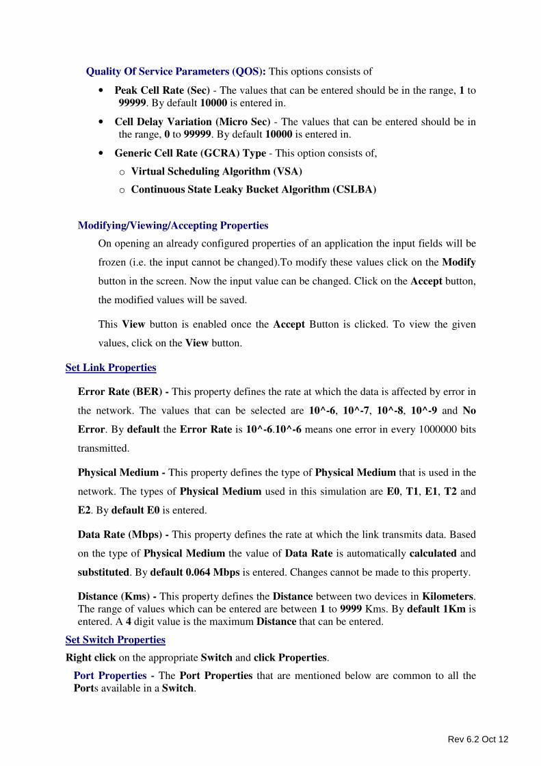
Quality Of Service Parameters (QOS): This options consists of
• Peak Cell Rate (Sec) - The values that can be entered should be in the range, 1 to
99999. By default 10000 is entered in.
• Cell Delay Variation (Micro Sec) - The values that can be entered should be in
the range, 0 to 99999. By default 10000 is entered in.
• Generic Cell Rate (GCRA) Type - This option consists of,
o Virtual Scheduling Algorithm (VSA)
o Continuous State Leaky Bucket Algorithm (CSLBA)
Modifying/Viewing/Accepting Properties
On opening an already configured properties of an application the input fields will be
frozen (i.e. the input cannot be changed).To modify these values click on the Modify
button in the screen. Now the input value can be changed. Click on the Accept button,
the modified values will be saved.
This View button is enabled once the Accept Button is clicked. To view the given
values, click on the View button.
Set Link Properties
Error Rate (BER) - This property defines the rate at which the data is affected by error in
the network. The values that can be selected are 10^-6, 10^-7, 10^-8, 10^-9 and No
Error. By default the Error Rate is 10^-6.10^-6 means one error in every 1000000 bits
transmitted.
Physical Medium - This property defines the type of Physical Medium that is used in the
network. The types of Physical Medium used in this simulation are E0, T1, E1, T2 and
E2. By default E0 is entered.
Data Rate (Mbps) - This property defines the rate at which the link transmits data. Based
on the type of Physical Medium the value of Data Rate is automatically calculated and
substituted. By default 0.064 Mbps is entered. Changes cannot be made to this property.
Distance (Kms) - This property defines the Distance between two devices in Kilometers.
The range of values which can be entered are between 1 to 9999 Kms. By default 1Km is
entered. A 4 digit value is the maximum Distance that can be entered.
Set Switch Properties
Right click on the appropriate Switch and click Properties.
Port Properties - The Port Properties that are mentioned below are common to all the
Ports available in a Switch.
Rev 6.2 Oct 12

Sorting technique - This property consists of the following options,
• Round Robin
• Priority. By default Priority is available.
• FIFO (First In First Out)
Buffer Size (KB) - This property specifies size of the buffer for that port on Switch.
Options available are � “8, 16, 32, 64, 128, 256, 512, 1024, 2048 and 4096”. Default
value is 8KB.
Remove Devices (or) Links
Remove Link - Right click on the appropriate Link and click Remove.
Remove ATM CPE - Right click on the appropriate ATM CPE and click Remove.
Remove ATM Switch - Right click on the appropriate ATM Switch and click Remove.
Note -
• First remove the connecting Link.
• Next remove the Switch / CPE. The removal of the Switch / CPE can be done after
the connecting link has been removed.
Simulate - After creating the Scenario the following steps need to be followed,
• Click on Validate button.
• Click on Simulate button.
• Select the Simulation End Time and then click on “OK” button to start the
Simulation.
NetSim - ATM
Sample Experiments - User can understand the internal working of ATM through these
sample experiments. Each sample experiment covers:
• Procedure
• Sample Inputs
• Output
• Comparison chart
• Inference
Rev 6.2 Oct 12
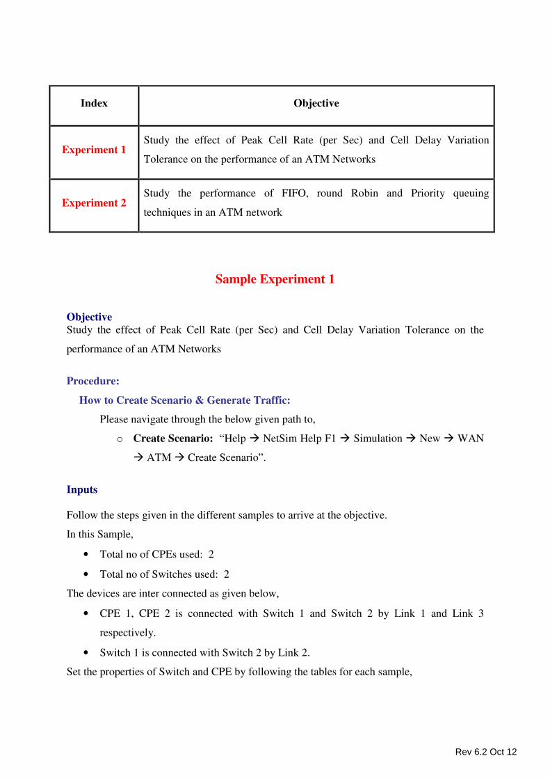
Index Objective
Experiment 1 Study the effect of Peak Cell Rate (per Sec) and Cell Delay Variation
Tolerance on the performance of an ATM Networks
Experiment 2 Study the performance of FIFO, round Robin and Priority queuing
techniques in an ATM network
Sample Experiment 1
Objective Study the effect of Peak Cell Rate (per Sec) and Cell Delay Variation Tolerance on the
performance of an ATM Networks
Procedure:
How to Create Scenario & Generate Traffic:
Please navigate through the below given path to,
o Create Scenario: “Help � NetSim Help F1 � Simulation � New � WAN
� ATM � Create Scenario”.
Inputs
Follow the steps given in the different samples to arrive at the objective.
In this Sample,
• Total no of CPEs used: 2
• Total no of Switches used: 2
The devices are inter connected as given below,
• CPE 1, CPE 2 is connected with Switch 1 and Switch 2 by Link 1 and Link 3
respectively.
• Switch 1 is connected with Switch 2 by Link 2.
Set the properties of Switch and CPE by following the tables for each sample,
Rev 6.2 Oct 12
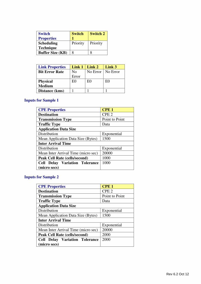
Switch
Properties
Switch
1
Switch 2
Scheduling
Technique
Priority Priority
Buffer Size (KB) 8 8
Link Properties Link 1 Link 2 Link 3
Bit Error Rate No
Error
No Error No Error
Physical
Medium
E0 E0 E0
Distance (kms) 1 1 1
Inputs for Sample 1
CPE Properties CPE 1
Destination CPE 2
Transmission Type Point to Point
Traffic Type Data
Application Data Size
Distribution Exponential
Mean Application Data Size (Bytes) 1500
Inter Arrival Time
Distribution Exponential
Mean Inter Arrival Time (micro sec) 20000
Peak Cell Rate (cells/second) 1000
Cell Delay Variation Tolerance
(micro secs)
1000
Inputs for Sample 2
CPE Properties CPE 1
Destination CPE 2
Transmission Type Point to Point
Traffic Type Data
Application Data Size
Distribution Exponential
Mean Application Data Size (Bytes) 1500
Inter Arrival Time
Distribution Exponential
Mean Inter Arrival Time (micro sec) 20000
Peak Cell Rate (cells/second) 2000
Cell Delay Variation Tolerance
(micro secs)
2000
Rev 6.2 Oct 12
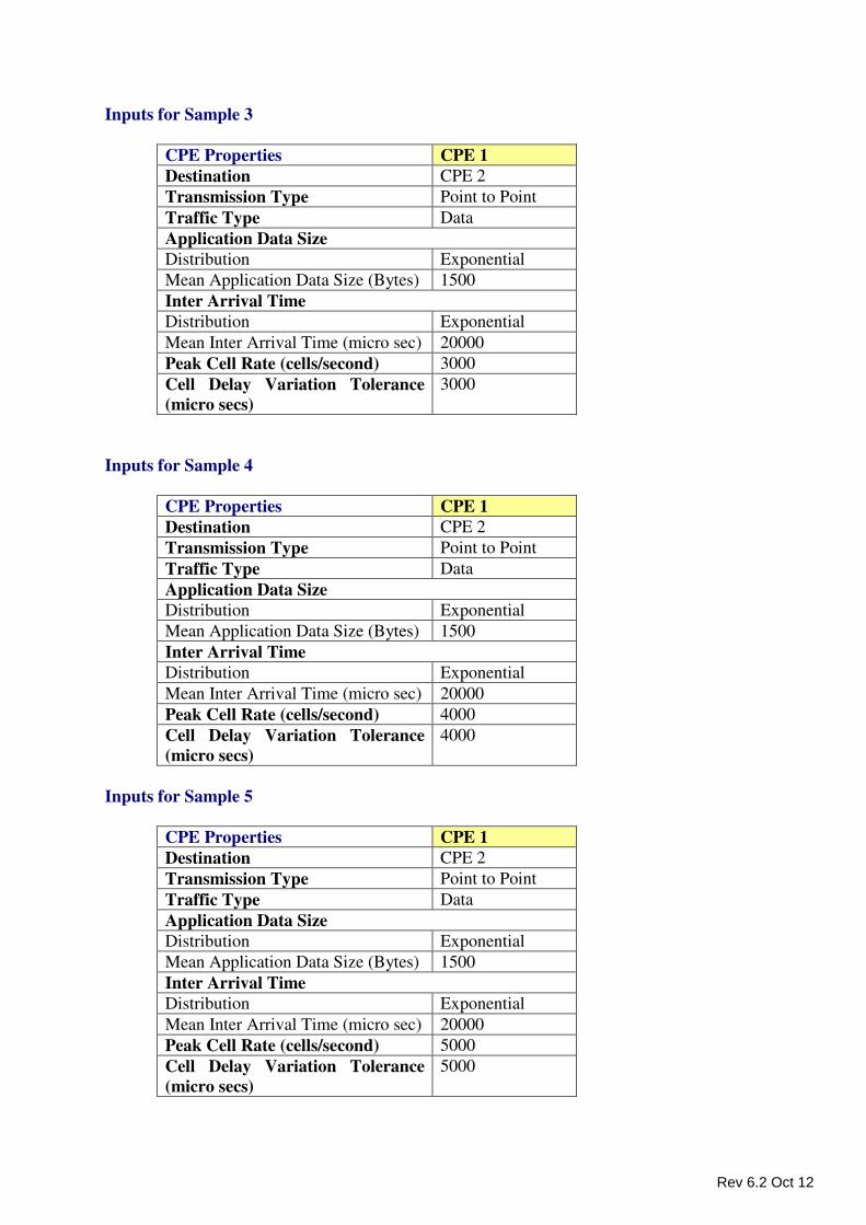
Inputs for Sample 3
CPE Properties CPE 1
Destination CPE 2
Transmission Type Point to Point
Traffic Type Data
Application Data Size
Distribution Exponential
Mean Application Data Size (Bytes) 1500
Inter Arrival Time
Distribution Exponential
Mean Inter Arrival Time (micro sec) 20000
Peak Cell Rate (cells/second) 3000
Cell Delay Variation Tolerance
(micro secs)
3000
Inputs for Sample 4
CPE Properties CPE 1
Destination CPE 2
Transmission Type Point to Point
Traffic Type Data
Application Data Size
Distribution Exponential
Mean Application Data Size (Bytes) 1500
Inter Arrival Time
Distribution Exponential
Mean Inter Arrival Time (micro sec) 20000
Peak Cell Rate (cells/second) 4000
Cell Delay Variation Tolerance
(micro secs)
4000
Inputs for Sample 5
CPE Properties CPE 1
Destination CPE 2
Transmission Type Point to Point
Traffic Type Data
Application Data Size
Distribution Exponential
Mean Application Data Size (Bytes) 1500
Inter Arrival Time
Distribution Exponential
Mean Inter Arrival Time (micro sec) 20000
Peak Cell Rate (cells/second) 5000
Cell Delay Variation Tolerance
(micro secs)
5000
Rev 6.2 Oct 12
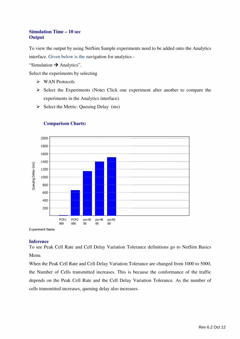
Simulation Time – 10 sec
Output
To view the output by using NetSim Sample experiments need to be added onto the Analytics
interface. Given below is the navigation for analytics -
“Simulation ���� Analytics”.
Select the experiments by selecting
� WAN Protocols
� Select the Experiments (Note: Click one experiment after another to compare the
experiments in the Analytics interface).
� Select the Metric: Queuing Delay (ms)
Comparison Charts:
Inference
To see Peak Cell Rate and Cell Delay Variation Tolerance definitions go to NetSim Basics
Menu.
When the Peak Cell Rate and Cell Delay Variation Tolerance are changed from 1000 to 5000,
the Number of Cells transmitted increases. This is because the conformance of the traffic
depends on the Peak Cell Rate and the Cell Delay Variation Tolerance. As the number of
cells transmitted increases, queuing delay also increases.
Rev 6.2 Oct 12
Sample Experiment 2
Objective Network performance analysis with an ATM switch implementing different scheduling
techniques like First in First out (FIFO), Priority, and
Round Robin
Theory In an ATM network, scheduling of cells is the major task of any ATM switch. Scheduling is
the process by which the ATM switch determines the sequence of flow of the cells in
network. The scheduling is done on various properties like service type, cell category, queue
length, arrival time etc.
First In First out (FIFO): FIFO is the simplest way of scheduling. As the name suggests, in
this technique, the preference is given to that cell which comes first in the queue irrespective
of its priority value. What comes next waits until the first finishes. The drawback of this
technique is that some cells of very high priority like audio service encounter extra delay that
is not ignorable.
Priority: In this technique, each cell is assigned a certain priority value based on its traffic
parameters. The scheduler checks the availability of highest priority cells and schedules them
before going for the lower priority cells. The drawback of this algorithm is that cells of
lowest priority starve for the resources when there are a large number of higher priority cells.
Round Robin: In this technique, the scheduler gives equal preference for all priority types.
Therefore, scheduler processes one cell of each priority type (If available) before going for
the next cell and cycles through them. Here starvation never occurs because no priority is
given. Round robin scheduling may not be desirable if QoS of the different priority type are
highly variable.
Procedure:
In this experiment, we are going to analyze the link Utilization (%) of the outgoing link from
an ATM switch
Rev 6.2 Oct 12
First In First Out (FIFO): In NetSim, Select Simulation�New�WAN�ATM
In the simulation environment window create the following scenario
How to Create Scenario & Generate Traffic:
Please navigate through the below given path to,
o Create Scenario: “Help � NetSim Help F1 � Simulation � New � WAN
� ATM � Create Scenario”.
Inputs
Follow the steps given in the different samples to arrive at the objective.
In all Samples,
• Total no of CPE used: 4
• Total no of ATM switch used: 2
The device are interconnected as given below
• CPE 1 is connected with switch 1 by link 1.
• CPE 2 is connected with switch 1 by link 2.
• CPE 3 is connected with switch 2 by link 4.
• CPE 4 is connected with switch 2 by link 5.
• Switch 1 and switch 2 are connected with link 3.
Set the properties for each device by following the tables,
Switch Properties Switch 1 Switch 2
Scheduling technique FIFO FIFO
Buffer size 4096 KB 4096 KB
CPE Properties CPE 1
Destination CPE 3
Transmission Type Point to Point
Traffic Type Data
Application Data Size
Distribution Constant
Mean Application Data Size (Bytes) 10000
Inter arrival time
Distribution Constant
Mean Inter-arrival time (Micro-sec) 10000
Generation rate (Mbps) 8
Scheduling FIFO
Rev 6.2 Oct 12
Peak cell rate (cells/sec) 99999
Cell delay Variation tolerance (Micro-sec) 99999
GCRA type VSA
CPE Properties CPE 2
Destination CPE 4
Transmission Type Point to Point
Traffic Type Voice
Codec Constant
Application Data Size (Bytes) 10000
Inter-arrival time (Micro-sec) 20000
Service Type CBR
Generation rate (Mbps) 4
Scheduling FIFO
Peak cell rate (cells/sec) 99999
Cell delay Variation tolerance (Micro-sec) 99999
GCRA type VSA
Link Properties Link 1 Link 2 Link 3 Link 4 Link 5
Bit Error Rate
(BER)
No Error No Error No Error No Error No Error
Physical medium E2 E2 E0 T1 T1
Data Rate (MbPS) 8.448 8.448 0.064 1.54 1.54
Distance 1 1 1 1 1
Simulation Time –10 Sec.
(Note: The Simulation Time can be selected only after doing the following two tasks,
o Set the properties of CPE and Switch,
o Then click on the Validate & Simulate button).
“Save” it, upon completion of the experiment.
Output:
Select the metrics Utilization and Delay report (Link). Note down the link utilization of link 4
and link 5.
Rev 6.2 Oct 12
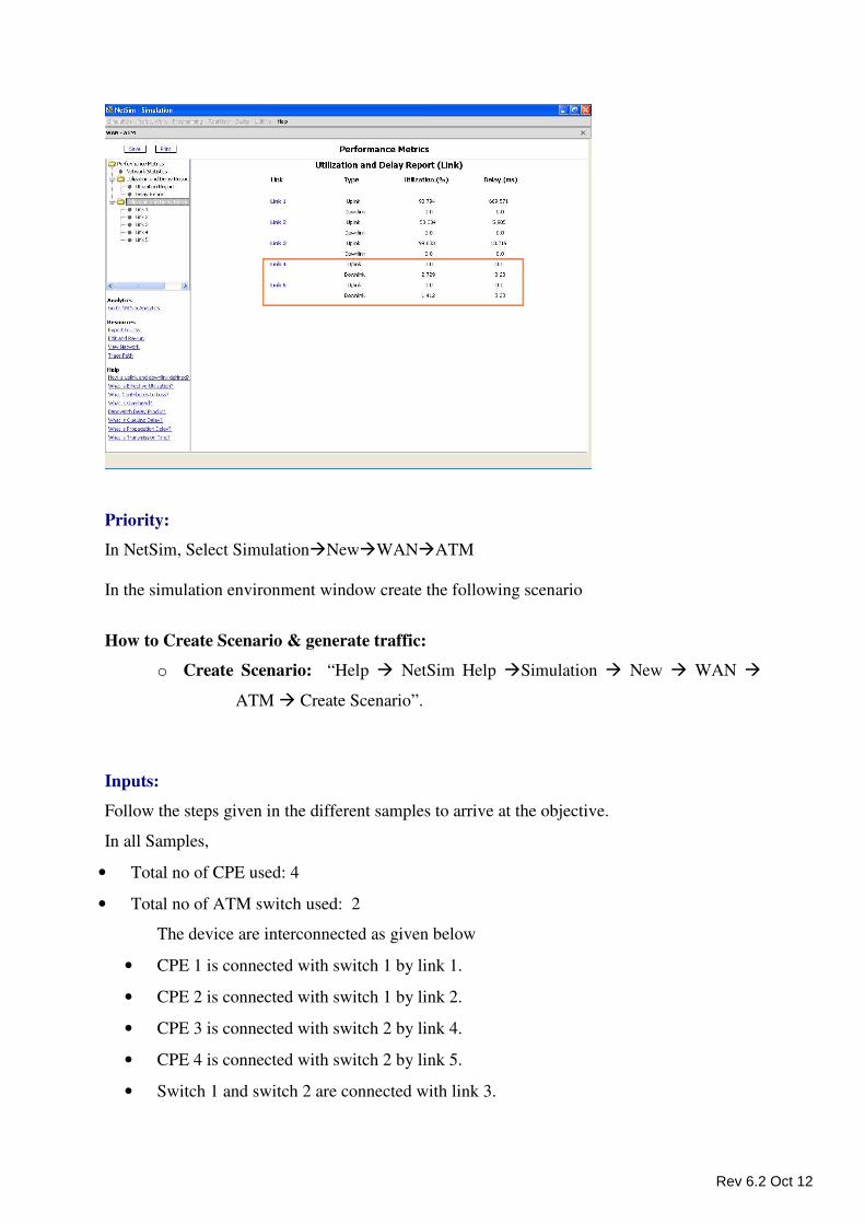
Priority:
In NetSim, Select Simulation�New�WAN�ATM
In the simulation environment window create the following scenario
How to Create Scenario & generate traffic:
o Create Scenario: “Help � NetSim Help �Simulation � New � WAN �
ATM � Create Scenario”.
Inputs:
Follow the steps given in the different samples to arrive at the objective.
In all Samples,
• Total no of CPE used: 4
• Total no of ATM switch used: 2
The device are interconnected as given below
• CPE 1 is connected with switch 1 by link 1.
• CPE 2 is connected with switch 1 by link 2.
• CPE 3 is connected with switch 2 by link 4.
• CPE 4 is connected with switch 2 by link 5.
• Switch 1 and switch 2 are connected with link 3.
Rev 6.2 Oct 12
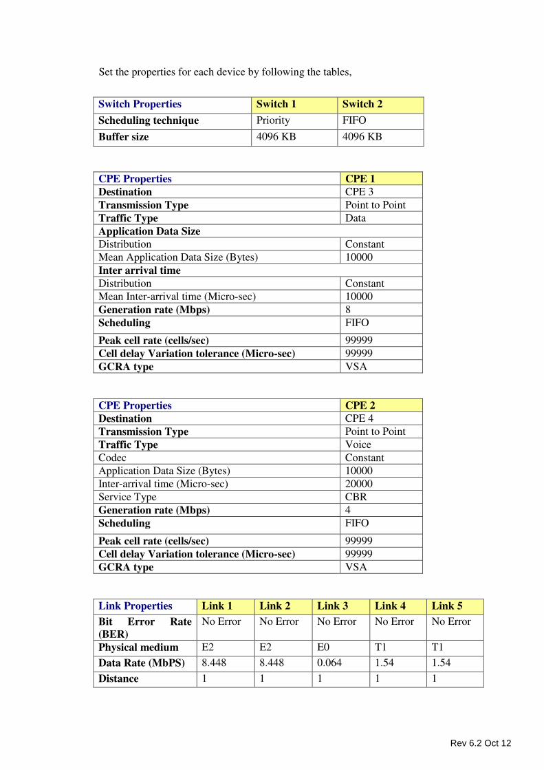
Set the properties for each device by following the tables,
Switch Properties Switch 1 Switch 2
Scheduling technique Priority FIFO
Buffer size 4096 KB 4096 KB
CPE Properties CPE 1
Destination CPE 3
Transmission Type Point to Point
Traffic Type Data
Application Data Size
Distribution Constant
Mean Application Data Size (Bytes) 10000
Inter arrival time
Distribution Constant
Mean Inter-arrival time (Micro-sec) 10000
Generation rate (Mbps) 8
Scheduling FIFO
Peak cell rate (cells/sec) 99999
Cell delay Variation tolerance (Micro-sec) 99999
GCRA type VSA
CPE Properties CPE 2
Destination CPE 4
Transmission Type Point to Point
Traffic Type Voice
Codec Constant
Application Data Size (Bytes) 10000
Inter-arrival time (Micro-sec) 20000
Service Type CBR
Generation rate (Mbps) 4
Scheduling FIFO
Peak cell rate (cells/sec) 99999
Cell delay Variation tolerance (Micro-sec) 99999
GCRA type VSA
Link Properties Link 1 Link 2 Link 3 Link 4 Link 5
Bit Error Rate
(BER)
No Error No Error No Error No Error No Error
Physical medium E2 E2 E0 T1 T1
Data Rate (MbPS) 8.448 8.448 0.064 1.54 1.54
Distance 1 1 1 1 1
Rev 6.2 Oct 12
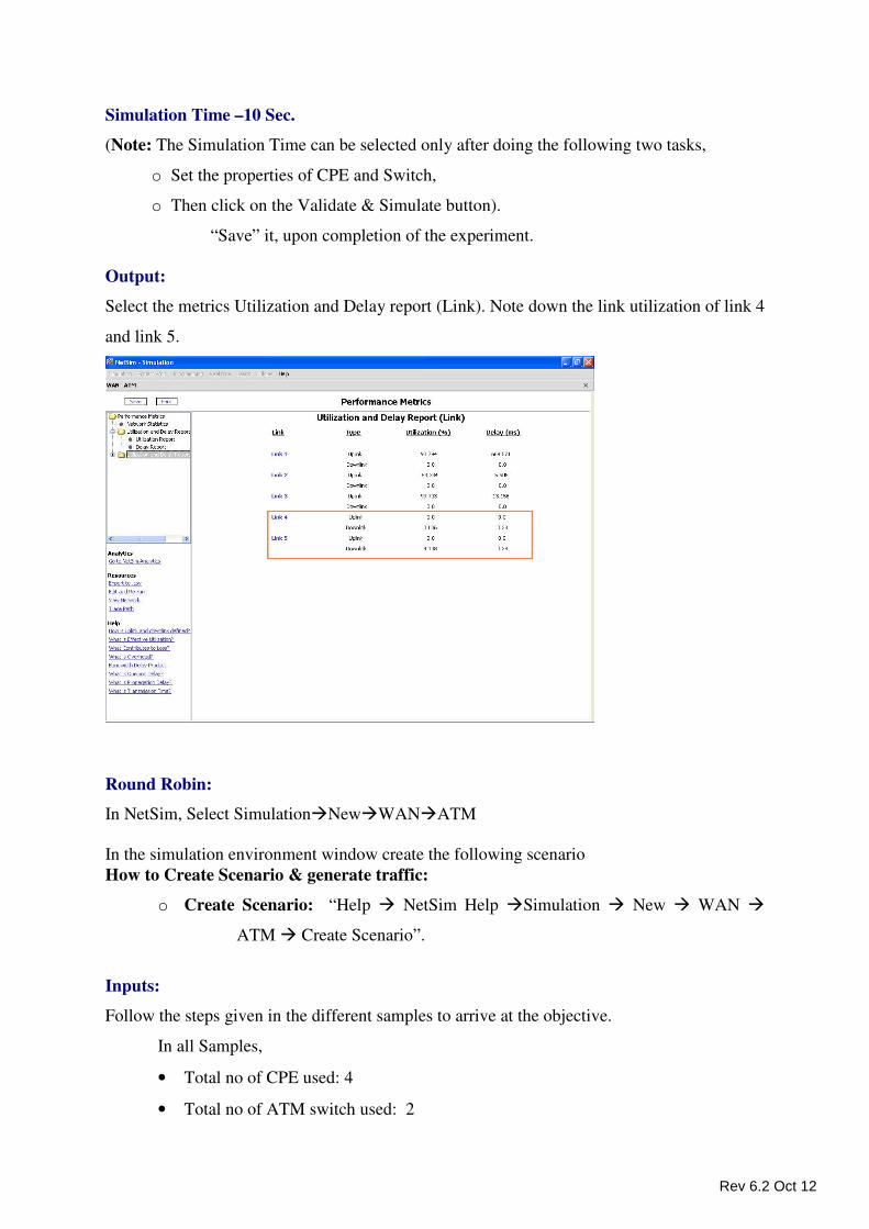
Simulation Time –10 Sec.
(Note: The Simulation Time can be selected only after doing the following two tasks,
o Set the properties of CPE and Switch,
o Then click on the Validate & Simulate button).
“Save” it, upon completion of the experiment.
Output:
Select the metrics Utilization and Delay report (Link). Note down the link utilization of link 4
and link 5.
Round Robin:
In NetSim, Select Simulation�New�WAN�ATM
In the simulation environment window create the following scenario
How to Create Scenario & generate traffic:
o Create Scenario: “Help � NetSim Help �Simulation � New � WAN �
ATM � Create Scenario”.
Inputs:
Follow the steps given in the different samples to arrive at the objective.
In all Samples,
• Total no of CPE used: 4
• Total no of ATM switch used: 2
Rev 6.2 Oct 12
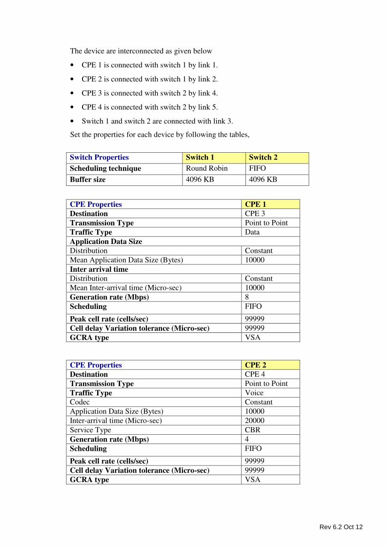
The device are interconnected as given below
• CPE 1 is connected with switch 1 by link 1.
• CPE 2 is connected with switch 1 by link 2.
• CPE 3 is connected with switch 2 by link 4.
• CPE 4 is connected with switch 2 by link 5.
• Switch 1 and switch 2 are connected with link 3.
Set the properties for each device by following the tables,
Switch Properties Switch 1 Switch 2
Scheduling technique Round Robin FIFO
Buffer size 4096 KB 4096 KB
CPE Properties CPE 1
Destination CPE 3
Transmission Type Point to Point
Traffic Type Data
Application Data Size
Distribution Constant
Mean Application Data Size (Bytes) 10000
Inter arrival time
Distribution Constant
Mean Inter-arrival time (Micro-sec) 10000
Generation rate (Mbps) 8
Scheduling FIFO
Peak cell rate (cells/sec) 99999
Cell delay Variation tolerance (Micro-sec) 99999
GCRA type VSA
CPE Properties CPE 2
Destination CPE 4
Transmission Type Point to Point
Traffic Type Voice
Codec Constant
Application Data Size (Bytes) 10000
Inter-arrival time (Micro-sec) 20000
Service Type CBR
Generation rate (Mbps) 4
Scheduling FIFO
Peak cell rate (cells/sec) 99999
Cell delay Variation tolerance (Micro-sec) 99999
GCRA type VSA
Rev 6.2 Oct 12
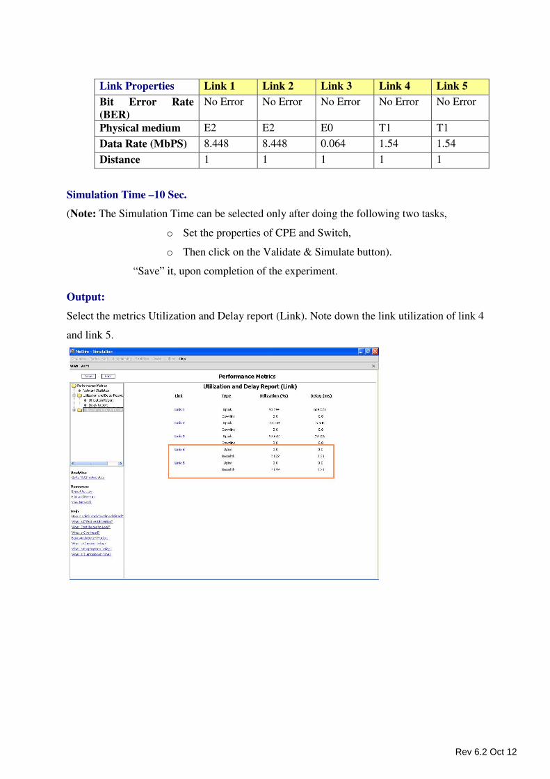
Link Properties Link 1 Link 2 Link 3 Link 4 Link 5
Bit Error Rate
(BER)
No Error No Error No Error No Error No Error
Physical medium E2 E2 E0 T1 T1
Data Rate (MbPS) 8.448 8.448 0.064 1.54 1.54
Distance 1 1 1 1 1
Simulation Time –10 Sec.
(Note: The Simulation Time can be selected only after doing the following two tasks,
o Set the properties of CPE and Switch,
o Then click on the Validate & Simulate button).
“Save” it, upon completion of the experiment.
Output:
Select the metrics Utilization and Delay report (Link). Note down the link utilization of link 4
and link 5.
Rev 6.2 Oct 12
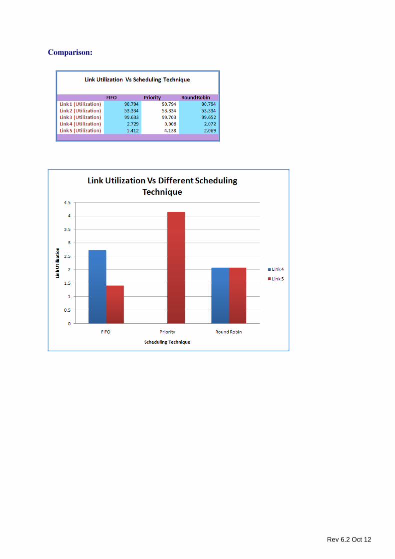
Comparison:
Rev 6.2 Oct 12
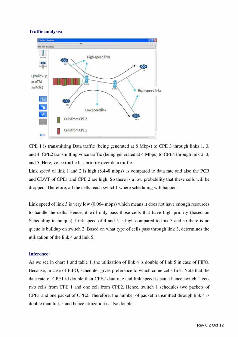
Traffic analysis:
CPE 1 is transmitting Data traffic (being generated at 8 Mbps) to CPE 3 through links 1, 3,
and 4. CPE2 transmitting voice traffic (being generated at 4 Mbps) to CPE4 through link 2, 3,
and 5. Here, voice traffic has priority over data traffic.
Link speed of link 1 and 2 is high (8.448 mbps) as compared to data rate and also the PCR
and CDVT of CPE1 and CPE 2 are high. So there is a low probability that these cells will be
dropped. Therefore, all the cells reach switch1 where scheduling will happens.
Link speed of link 3 is very low (0.064 mbps) which means it does not have enough resources
to handle the cells. Hence, it will only pass those cells that have high priority (based on
Scheduling technique). Link speed of 4 and 5 is high compared to link 3 and so there is no
queue is buildup on switch 2. Based on what type of cells pass through link 3, determines the
utilization of the link 4 and link 5.
Inference:
As we see in chart 1 and table 1, the utilization of link 4 is double of link 5 in case of FIFO.
Because, in case of FIFO, scheduler gives preference to which come cells first. Note that the
data rate of CPE1 id double than CPE2 data rate and link speed is same hence switch 1 gets
two cells from CPE 1 and one cell from CPE2. Hence, switch 1 schedules two packets of
CPE1 and one packet of CPE2. Therefore, the number of packet transmitted through link 4 is
double than link 5 and hence utilization is also double.
Rev 6.2 Oct 12
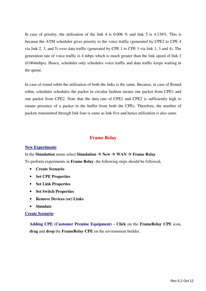
In case of priority, the utilization of the link 4 is 0.006 % and link 5 is 4.138%. This is
because the ATM scheduler gives priority to the voice traffic (generated by CPE2 to CPE 4
via link 2, 3, and 5) over data traffic (generated by CPE 1 to CPE 3 via link 1, 3 and 4). The
generation rate of voice traffic is 4 mbps which is much greater than the link speed of link 3
(0.064mbps). Hence, scheduler only schedules voice traffic and data traffic keeps waiting in
the queue.
In case of round robin the utilization of both the links is the same. Because, in case of Round
robin, scheduler schedules the packet in circular fashion means one packet from CPE1 and
one packet from CPE2. Note that the data rate of CPE1 and CPE2 is sufficiently high to
ensure presence of a packet in the buffer from both the CPEs. Therefore, the number of
packets transmitted through link four is same as link five and hence utilization is also same.
Frame Relay
New Experiments
In the Simulation menu select Simulation � New � WAN � Frame Relay
To perform experiments in Frame Relay, the following steps should be followed,
• Create Scenario
• Set CPE Properties
• Set Link Properties
• Set Switch Properties
• Remove Devices (or) Links
• Simulate
Create Scenario
Adding CPE (Customer Premise Equipment) - Click on the FrameRelay CPE icon,
drag and drop the FrameRelay CPE on the environment builder.
Rev 6.2 Oct 12
Adding Switch - Click on the Switch icon, drag and drop the Switch on the environment
builder. By default a Switch has eight ports.
Establishing Connections between FrameRelay CPE and Switch - The steps for to be
followed are as follows,
• The connections between the two FrameRelay CPEs cannot be made in the network.
• On clicking the two devices connection can be made.
• The connection possibilities are,
o CPE to Switch and
o Switch to Switch.
Set CPE (Customer Premises Equipment) Properties
Right Click on the appropriate node to select Properties. Inside the properties’ window click
on Application 1 to modify its properties.
Transmission Type
This indicates the type of transmission made by this session, only Point to Point
Transmission can be made.
Destination
This property indicates the Destination CPE.
Traffic Type
This property indicates the type of traffic. The traffic can either be Voice or Data.
Voice
Codec
Codec is the component of any voice system that translates between analog speech and
the bits used to transmit them. Every codec transmits a burst of data in a packet that can
be reconstructed into voice. Five different standards of voice codec’s are given which
can be selected depending on the variations required.
Service Type
• CBR - CBR stands for Constant Bit Rate. Packets of constant size are generated at
constant inter arrival times.
• VBR - VBR stands for Variable Bit Rate. The two types of Suppression Model that
can be selected are,
• Deterministic
• Markov Chain
Rev 6.2 Oct 12
Click OK to accept the user entered values. Click on the close button at the top right
corner to exit the screen.
Data
Packet Size
Distribution: The options available for distribution are,
• Constant
• Exponential
Mean Packet Size (Bytes): Sets the size of the packets being generated by the chosen
distribution. The range of values that can be entered are between 65 to 1500 bytes. By
default 1500 bytes is entered.
Inter Arrival Time
This indicates the time gap between packets.
Distribution: The options available for distribution are,
• Constant
• Exponential
• Uniform
Mean Inter Arrival Time: Enter the average inter-arrival time between packets. A
lower inter-arrival time would lead to a higher generation rate and the vice versa. The
range of values that can be entered are between 1000 to 20000 Micro Sec. By default
20000 Micro Sec is entered.
Click OK to accept the user entered values. Click on the close button at the top right
corner to exit the screen.
Data Link Layer
CIR (Committed Information Rate) Value: This option consists of
• 0.056 (by default this value is set)
• 0.112
• 0.224
• 0.448
Modifying/Viewing/Accepting Properties
On opening an already configured properties of an application the input fields will be
frozen (i.e. the input cannot be changed).To modify these values click on the Modify
button in the screen. Now the input value can be changed. Click on the Accept button,
the modified values will be saved.
This View button is enabled once the Accept Button is clicked. To view the given
values, click on the View button.
Rev 6.2 Oct 12
Set Link Properties
Error Rate (BER) - This property defines the rate at which the data is affected by error
in the network. The values that can be selected are 10^-6, 10^-7, 10^-8, 10^-9 and No
Error. By default the Error Rate is 10^-6.10^-6 means one error in every 1000000 bits
transmitted.
Physical Medium - This property defines the type of Physical Medium that is used in
the network. The types of Physical Medium used in this simulation are E0, T1, E1, T2
and E2. By default E0 is entered.
Data Rate (Mbps) - This property defines the rate at which the link transmits data. Based
on the type of Physical Medium the value of Data Rate is automatically calculated and
substituted. By default 0.064 Mbps is entered. Changes cannot be made to this property.
Distance (Kms) - This property defines the Distance between two devices in
Kilometers. The range of values which can be entered are between 1 to 9999 Kms.
By default 1Km is entered. A 4 digit value is the maximum Distance that can be
entered.
Set Switch Properties
Right click on the appropriate Switch and click Properties.
Port Properties - The Port Properties that are mentioned below are common to all the
Ports available in a Switch.
Buffer Size (KB) - This property specifies size of the buffer for that port on Switch.
Options available are � “8, 16, 32, 64, 128, 256, 512, 1024, 2048 and 4096”. Default
value is 8KB.
Remove Devices (or) Links
Remove Link - Right click on the appropriate Link and click Remove.
Remove FrameRelay CPE - Right click on the appropriate FrameRelay CPE and click
Remove.
Remove FrameRelay Switch - Right click on the appropriate FrameRelay Switch and
click Remove.
Note -
• First remove the connecting Link.
• Next remove the Switch / CPE. The removal of the Switch / CPE can be done after
the connecting link has been removed.
Rev 6.2 Oct 12
Simulate - After creating the Scenario the following steps need to be followed,
• Click on Validate button.
• Click on Simulate button.
• Select the Simulation End Time and then click on “OK” button to start the
Simulation.
BGP
New Experiments
In the Simulation menu select Simulation � New � WAN � IP Routing � BGP
To perform experiments in Routing, the following steps should be followed,
• Create Scenario
• Set CPE Properties
• Set Link Properties
• Set Router Properties
• Remove Devices (or) Links
• Simulate
Create Scenario
Adding CPE (Customer Premise Equipment) - Click on the Router CPE icon, drag
and drop the Router CPE on the environment builder.
Adding Border Router - Click on the Border Router icon, drag and drop the Border
Router on the environment builder. An Autonomous system is created by default.
Maximum you can have 3 Autonomous systems in a single scenario.
Adding Internal Router - Click on the Internal Router icon, drag and drop the
Internal Router onto the Autonomous systems created. By default a Router has eight
ports.
Establishing Connections between Router CPE and Router - The steps for to be
followed are as follows,
• The connections between the two Router CPEs cannot be made in the network.
• On clicking the two devices connection can be made.
• The connection possibilities are,
o CPE to Internal Router
o CPE to Border Router
Rev 6.2 Oct 12
o Internal Router to Internal Router
o Internal Router to Border Router
o Border Router to Border Router
Set CPE (Customer Premises Equipment) Properties
Right Click on the appropriate node to select Properties. Inside the properties’ window click
on Application 1 to modify its properties.
Transmission Type
This indicates the type of transmission made by this session, only Point to Point
Transmission can be made.
Destination
This property indicates the Destination CPE.
Traffic Type
This property indicates the type of traffic. The traffic can either be Voice or Data.
Voice
Codec
Codec is the component of any voice system that translates between analog speech
and the bits used to transmit them. Every codec transmits a burst of data in a packet
that can be reconstructed into voice. Five different standards of voice codec’s are
given which can be selected depending on the variations required.
Service Type
• CBR - CBR stands for Constant Bit Rate. Packets of constant size are generated
at constant inter arrival times.
• VBR - VBR stands for Variable Bit Rate. The two types of Suppression Model
that can be selected are,
• Deterministic
• Markov Chain
Click OK to accept the user entered values. Click on the close
button at the top right corner to exit the screen.
Data
Packet Size
Distribution: The options available for distribution are,
Rev 6.2 Oct 12
• Constant
• Exponential
Mean Packet Size (Bytes): Sets the size of the packets being generated by the chosen
distribution. The range of values that can be entered are between 10 to 10000 bytes.
By default 1472 bytes is entered.
Inter Arrival Time
This indicates the time gap between packets.
Distribution : The options available for distribution are,
• Constant
• Exponential
• Uniform
Mean Inter Arrival Time: Enter the average inter-arrival time between packets. A
lower inter-arrival time would lead to a higher generation rate and the vice versa. The
range of values that can be entered are between 1000 to 20000 Micro Sec. By default
20000 Micro Sec is entered.
Click OK to accept the user entered values. Click on the close button at the top right
corner to exit the screen.
Network Layer
IP Address: Set the IP Address of the Nodes by selecting the appropriate values.
Subnet Mask: Give the valid values in this field.
Priority
Click to select the Priority. Its Values are Low, Normal, Medium and High. By
default the Priority is Low.
Modifying/Viewing/Accepting Properties
On opening an already configured properties of an application the input fields will
be frozen (i.e. the input cannot be changed).To modify these values click on the
Modify button in the screen. Now the input value can be changed. Click on the
Accept button, the modified values will be saved.
This View button is enabled once the Accept Button is clicked. To view the given
values, click on the View button.
Rev 6.2 Oct 12
Set Link Properties
CPE to Internal Router and CPE to Border Router Link - To set the property values
right click the Link between CPE to Internal Router or CPE to Border Router and select
Properties option. There are 4 property options that are available. They are,
Error Rate (BER) - This property defines the rate at which the data is affected by
error in the network. The values that can be selected are 10^-6, 10^-7, 10^-8, 10^-9
and No Error. By default the Error Rate is 10^-6.10^-6 means one error in every
1000000 bits transmitted.
Physical Medium - This property defines the type of Physical Medium that is used
in the network. The types of Physical Medium used in this simulation are E0, T1,
E1, T2 and E2. By default E0 is entered.
Data Rate (Mbps) - This property defines the rate at which the link transmits data.
Based on the type of Physical Medium the value of Data Rate is automatically
calculated and substituted. By default 0.064 Mbps is entered. Changes cannot be
made to this property.
Distance (Kms) - This property defines the Distance between two devices in
Kilometers. By default 1Km is entered. A 4 digit value is the maximum Distance
that can be entered.
Link Weight - This property defines the weight of the Link. This property depends
on the Protocol Type selected inside Router Properties (i.e. If the Protocol Type is
RIP then the default value is 1 and changes cannot be made. If the Protocol Type is
OSPF, then any value less than 1000 would be accepted and by default the value
entered is 1).
Internal Router to Internal Router and Internal Router to Border Router Link - To
change the property values right click the Link between Internal Router to Internal
Router or Internal Router to Border Router and click Properties. There are 4 options
for which changes can be made. They are,
Error Rate (BER) - This property defines the rate at which the data is affected by
error in the network. The values that can be selected are 10^-6, 10^-7, 10^-8, 10^-9
and No Error. By default the Error Rate is 10^-6.10^-6 means one error in every
1000000 bits transmitted.
Rev 6.2 Oct 12
Physical Medium - This property defines the type of Physical Medium used in the
network. The Physical Medium that is used in connecting 2 Routers is a CAT5.
Data Rate (Mbps) - This property defines the rate at which the Link transmits data.
The two types of Data Rate that can be selected are, 10 and 100 Mbps. By default
10Mbps is entered.
Distance (km) - This property defines the Distance between two devices in
Kilometers. By default 1Km is entered. A 4 digit value is the maximum Distance
that can be entered.
Link Weight - This property defines the weight of the Link. This property depends
on the Protocol Type selected inside Router Properties (i.e. if the Protocol Type is
RIP then the default value is 1 and changes cannot be made. If the Protocol Type is
OSPF, then any value less than 1000 would be accepted and by default the value
entered is 1).
Border Router to Border Router Link - To change the property values right click the
Link between Border Router to Border Router and click Properties. There are 4
options for which changes can be made. They are,
Error Rate (BER) - This property defines the rate at which the data is affected by
error in the network. The values that can be selected are 10^-6, 10^-7, 10^-8, 10^-9
and No Error. By default the Error Rate is 10^-6.10^-6 means one error in every
1000000 bits transmitted.
Physical Medium - This property defines the type of Physical Medium used in the
network. The Physical Medium that is used in connecting 2 Routers is a CAT5.
Data Rate (Mbps) - This property defines the rate at which the Link transmits data.
The Data Rate of 1000Mbps is fixed here.
Distance (km) - This property defines the Distance between two devices in
Kilometers. By default 1Km is entered. A 4 digit value is the maximum Distance
that can be entered.
Link Weight - This property defines the weight of the Link. This property depends
on the Protocol Type selected inside Router Properties (i.e. if the Protocol Type is
RIP then the default value is 1 and changes cannot be made. If the Protocol Type is
Rev 6.2 Oct 12
OSPF, then any value less than 1000 would be accepted and by default the value
entered is 1).
Set Router Properties
Internal Router Properties - To change any property, right click on the appropriate
Router to get the option window and click Properties.
Ports Properties - The number of ports available in a Router are 8. For each Port in a
Router the following properties are available,
IP Address - The IP Address must be filled up with a valid IP Address. By default
the IP Address that would be filled is “10.1.5.1”.
Subnet Mask - By default the value that is found in the Subnet Mask field is
“255.255.255.0”.
Connected To - This property gives the Router CPE that is connected to that Port
(i.e. If the CPE1 is connected to Port1, then when Port1 is selected CPE1 would be
displayed).
Routing Properties
Buffer Size (KB) - This property defines the Buffer size that should be selected.
Click on the drop down button to avail the values. The values that are available are,
“8, 16, 32, 64, 128, 256, 512, 1024, 2048 and 4096 (KB)”. 8KB is the default value.
Scheduling Type - Here the type of scheduler required can be selected. The 2 types
of Scheduling Type are Priority and FIFO. By default Priority is available.
Routing Protocol - The options available under Routing Protocol are,
Protocol Type - The type of protocol to be used can be selected. There are two
options for this. One is RIP and other one is OSPF.
If you select RIP as your Protocol Type, following options are available.
Periodic Time (1 to 30 sec) - The value that must be entered here should be within the
limit given. By default 30 seconds is entered.
Expiration Time (sec) - Here the value that must be entered should be greater than that
of Periodic Time and the maximum value is 180 sec. By default the value entered is
180 seconds.
Rev 6.2 Oct 12
Garbage collection Time (1 to 120 sec) - Here the value that can be entered is between 1
to 120 seconds. By default the value entered is 120 seconds.
If you select OSPF as your Protocol Type, the following options are available for you.
Router Priority (0 to 256) - Here the range of value that can be entered is 0 to 256. By
default the value entered is 256.
LSA Refresh Time (sec) - By default the value given here is 150 seconds.
LSA Max Age (sec) - By default the value given here is 300 seconds.
Data Link Layer - The options available under this property is,
Protocol Type - By default the Protocol Type found here is Ethernet. Here changes
cannot be made
Border Router Properties - To change any property, right click on the appropriate Router
to get the option window and click Properties.
Ports Properties - The number of ports available in a Router are 8. For each Port in a
Router the following properties are available,
IP Address - The IP Address must be filled up with a valid IP Address. By default the
IP Address that would be filled is “10.1.5.1”.
Subnet Mask - By default the value that is found in the Subnet Mask field is
“255.255.255.0”.
Connected To - This property gives the Router CPE that is connected to that Port (i.e.
If the CPE1 is connected to Port1, then when Port1 is selected CPE1 would be
displayed).
Routing Properties
Buffer Size (KB) - This property defines the Buffer size that should be selected. Click
on the drop down button to avail the values. The values that are available are, “8, 16, 32,
64, 128, 256, 512, 1024, 2048 and 4096 (KB)”. 8KB is the default value.
Scheduling Type - Here the type of scheduler required can be selected. The 2 types of
Scheduling Type are Priority and FIFO. By default Priority is available.
Rev 6.2 Oct 12
Routing Protocol – Let say the selected BGP Router has 2 ports. One connected to Router
(Internal / Border) of same Autonomous system (AS) and another connected to Router
(Internal / Border) of different AS.
The options available under Routing Protocol if the port connecting to Routers of same AS
are,
Protocol Type - The type of protocol to be used can be selected. There are two options
for this. One is RIP and other one is OSPF.
If you select RIP as your Protocol Type, following options are available.
Periodic Time (1 to 30 sec) - The value that must be entered here should be within the
limit given. By default 30 seconds is entered.
Expiration Time (sec) - Here the value that must be entered should be greater than that
of Periodic Time and the maximum value is 180 sec. By default the value entered is
180 seconds.
Garbage collection Time (1 to 120 sec) - Here the value that can be entered is between 1
to 120 seconds. By default the value entered is 120 seconds.
If you select OSPF as your Protocol Type, the following options are available for you.
Router Priority (0 to 256) - Here the range of value that can be entered is 0 to 256. By
default the value entered is 256.
LSA Refresh Time (sec) - By default the value given here is 150 seconds.
LSA Max Age (sec) - By default the value given here is 300 seconds.
The options available under Routing Protocol if the port connecting to Routers of
different AS are,
Protocol Type - The type of protocol to be used can be selected. By default Protocol
Type is BGP 4.
The following options are available for BGP protocol.
Local Preference: The possible values here are 100, 200, 300, 400 and 500. Default
value is 100 here.
MED (Multiple Exit Discriminator): Here the range of value that can be entered is from
0 to 100. Default value is 0 here.
Rev 6.2 Oct 12
Data Link Layer - The options available under this property is,
Protocol Type - By default the Protocol Type found here is Ethernet. Here changes
cannot be made
Remove Devices (or) Links
Remove Link - Right click on the appropriate Link and click Remove.
Remove Router CPE - Right click on the appropriate Router CPE and click Remove.
Remove Internal & Border Router - Right click on the appropriate Router and click
Remove.
Note -
• First remove the connecting Link.
• Next remove the Router / CPE. The removal of the Router / CPE can be done after
the connecting link has been removed
Simulate - After creating the Scenario the following steps need to be followed,
• Click on Validate button.
• Click on Simulate button.
• Select the Simulation End Time and then click on “OK” button to start the
Simulation.
NetSim - BGP
Sample Experiments - User can understand the working of BGP and formation of BGP
Routing Tables through this sample experiment. The sample experiment covers:
• Procedure
• Sample Inputs
• Output
• Inference
Index Objective
Experiment 1 Study the working of BGP and formation of BGP Routing table.
Rev 6.2 Oct 12
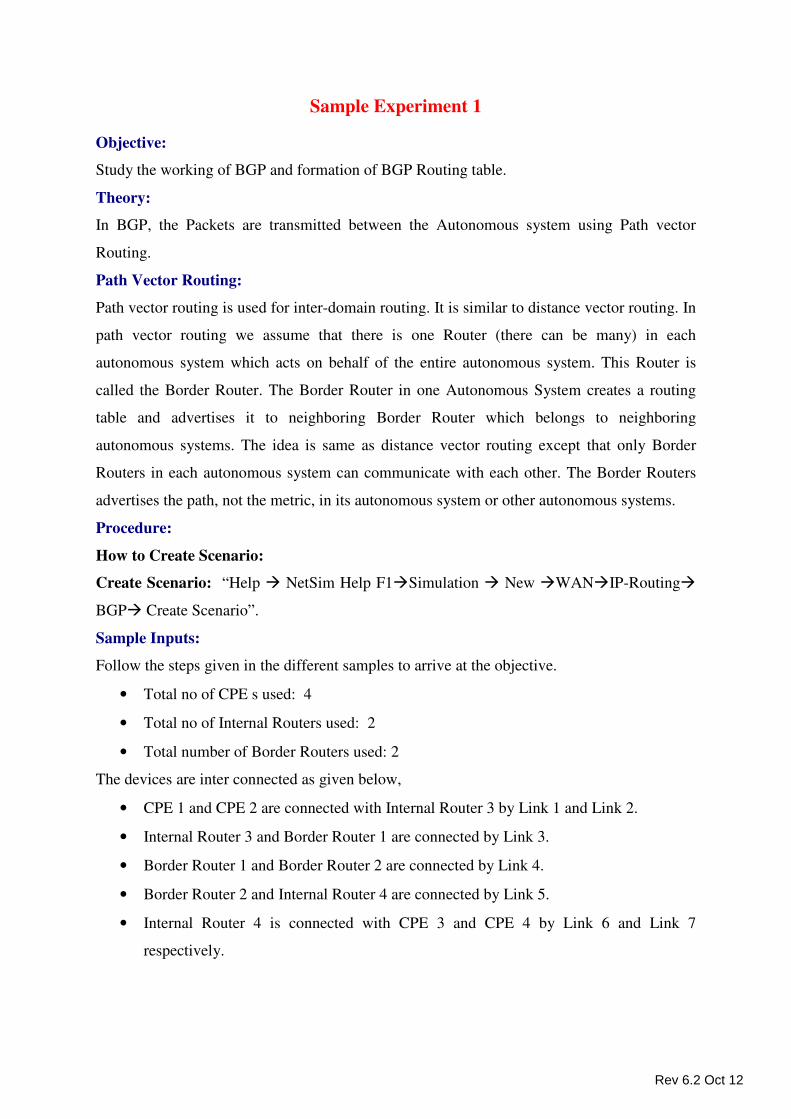
Sample Experiment 1
Objective:
Study the working of BGP and formation of BGP Routing table.
Theory:
In BGP, the Packets are transmitted between the Autonomous system using Path vector
Routing.
Path Vector Routing:
Path vector routing is used for inter-domain routing. It is similar to distance vector routing. In
path vector routing we assume that there is one Router (there can be many) in each
autonomous system which acts on behalf of the entire autonomous system. This Router is
called the Border Router. The Border Router in one Autonomous System creates a routing
table and advertises it to neighboring Border Router which belongs to neighboring
autonomous systems. The idea is same as distance vector routing except that only Border
Routers in each autonomous system can communicate with each other. The Border Routers
advertises the path, not the metric, in its autonomous system or other autonomous systems.
Procedure:
How to Create Scenario:
Create Scenario: “Help � NetSim Help F1�Simulation � New �WAN�IP-Routing�
BGP� Create Scenario”.
Sample Inputs:
Follow the steps given in the different samples to arrive at the objective.
• Total no of CPE s used: 4
• Total no of Internal Routers used: 2
• Total number of Border Routers used: 2
The devices are inter connected as given below,
• CPE 1 and CPE 2 are connected with Internal Router 3 by Link 1 and Link 2.
• Internal Router 3 and Border Router 1 are connected by Link 3.
• Border Router 1 and Border Router 2 are connected by Link 4.
• Border Router 2 and Internal Router 4 are connected by Link 5.
• Internal Router 4 is connected with CPE 3 and CPE 4 by Link 6 and Link 7
respectively.
Rev 6.2 Oct 12
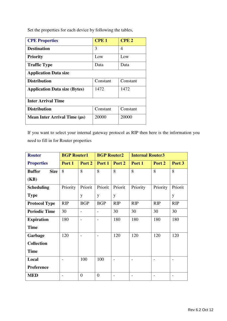
Set the properties for each device by following the tables,
If you want to select your internal gateway protocol as RIP then here is the information you
need to fill in for Router properties
CPE Properties CPE 1 CPE 2
Destination 3 4
Priority Low Low
Traffic Type Data Data
Application Data size
Distribution Constant Constant
Application Data size (Bytes) 1472 1472
Inter Arrival Time
Distribution Constant Constant
Mean Inter Arrival Time (µs) 20000 20000
Router
Properties
BGP Router1 BGP Router2 Internal Router3
Port 1 Port 2 Port 1 Port 2 Port 1 Port 2 Port 3
Buffer Size
(KB)
8 8 8 8 8 8 8
Scheduling
Type
Priority Priorit
y
Priorit
y
Priorit
y
Priority Priority Priorit
y
Protocol Type RIP BGP BGP RIP RIP RIP RIP
Periodic Time 30 - - 30 30 30 30
Expiration
Time
180 - - 180 180 180 180
Garbage
Collection
Time
120 - - 120 120 120 120
Local
Preference
- 100 100 - - - -
MED - 0 0 - - - -
Rev 6.2 Oct 12
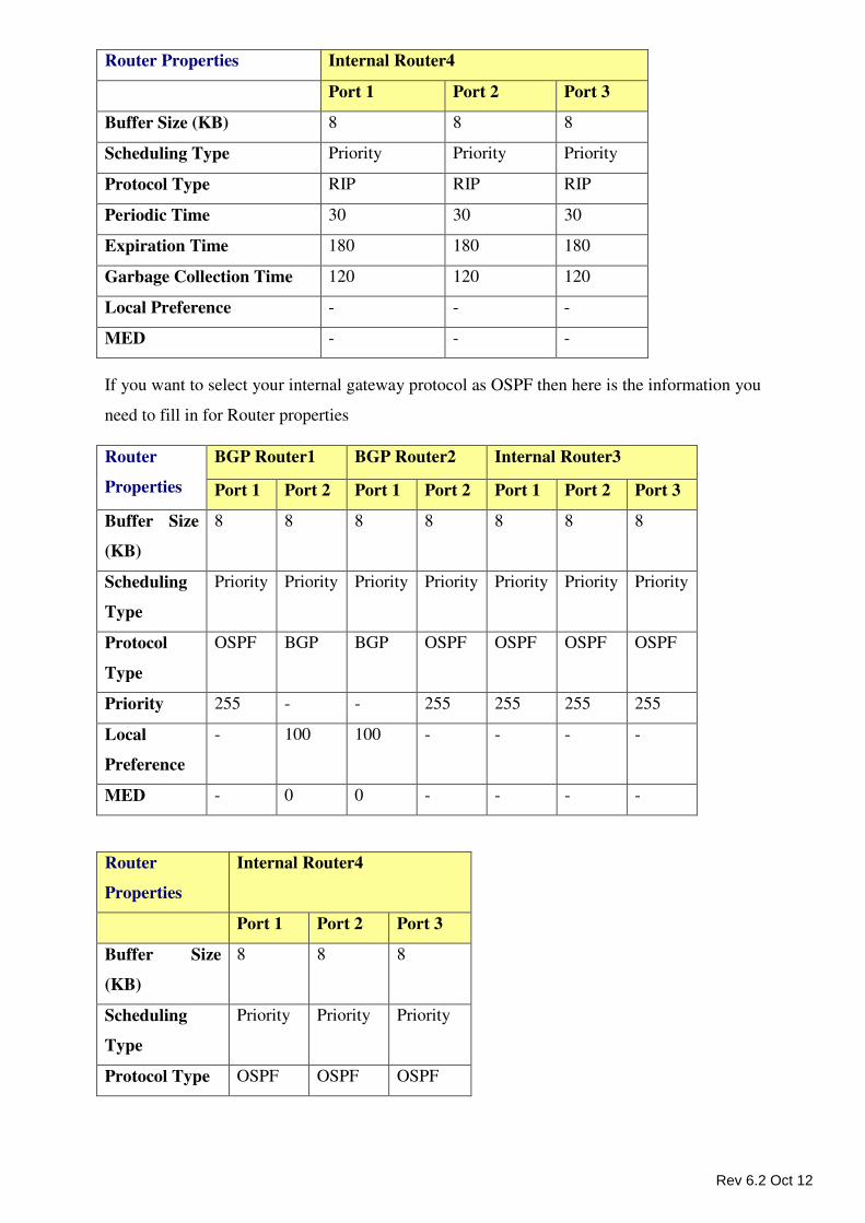
If you want to select your internal gateway protocol as OSPF then here is the information you
need to fill in for Router properties
Router Properties Internal Router4
Port 1 Port 2 Port 3
Buffer Size (KB) 8 8 8
Scheduling Type Priority Priority Priority
Protocol Type RIP RIP RIP
Periodic Time 30 30 30
Expiration Time 180 180 180
Garbage Collection Time 120 120 120
Local Preference - - -
MED - - -
Router
Properties
BGP Router1 BGP Router2 Internal Router3
Port 1 Port 2 Port 1 Port 2 Port 1 Port 2 Port 3
Buffer Size
(KB)
8 8 8 8 8 8 8
Scheduling
Type
Priority Priority Priority Priority Priority Priority Priority
Protocol
Type
OSPF BGP BGP OSPF OSPF OSPF OSPF
Priority 255 - - 255 255 255 255
Local
Preference
- 100 100 - - - -
MED - 0 0 - - - -
Router
Properties
Internal Router4
Port 1 Port 2 Port 3
Buffer Size
(KB)
8 8 8
Scheduling
Type
Priority Priority Priority
Protocol Type OSPF OSPF OSPF
Rev 6.2 Oct 12
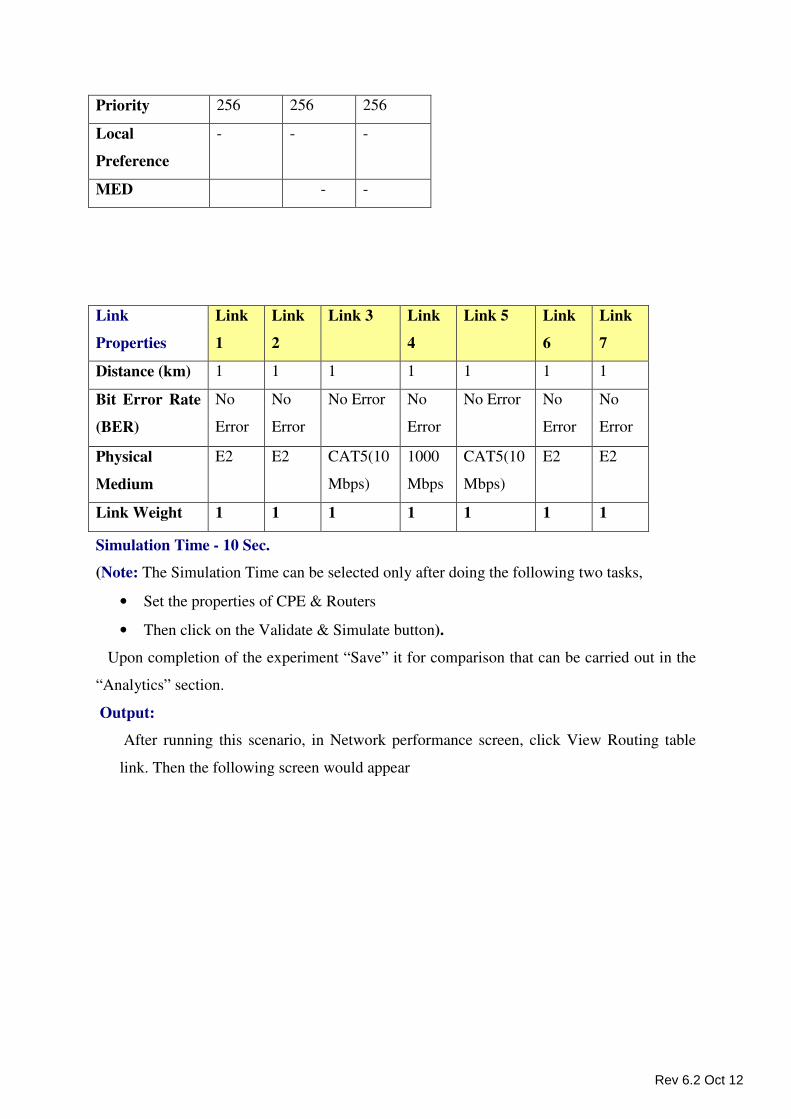
Simulation Time - 10 Sec.
(Note: The Simulation Time can be selected only after doing the following two tasks,
• Set the properties of CPE & Routers
• Then click on the Validate & Simulate button).
Upon completion of the experiment “Save” it for comparison that can be carried out in the
“Analytics” section.
Output:
After running this scenario, in Network performance screen, click View Routing table
link. Then the following screen would appear
Priority 256 256 256
Local
Preference
- - -
MED - -
Link
Properties
Link
1
Link
2
Link 3 Link
4
Link 5 Link
6
Link
7
Distance (km) 1 1 1 1 1 1 1
Bit Error Rate
(BER)
No
Error
No
Error
No Error No
Error
No Error No
Error
No
Error
Physical
Medium
E2 E2 CAT5(10
Mbps)
1000
Mbps
CAT5(10
Mbps)
E2 E2
Link Weight 1 1 1 1 1 1 1
Rev 6.2 Oct 12
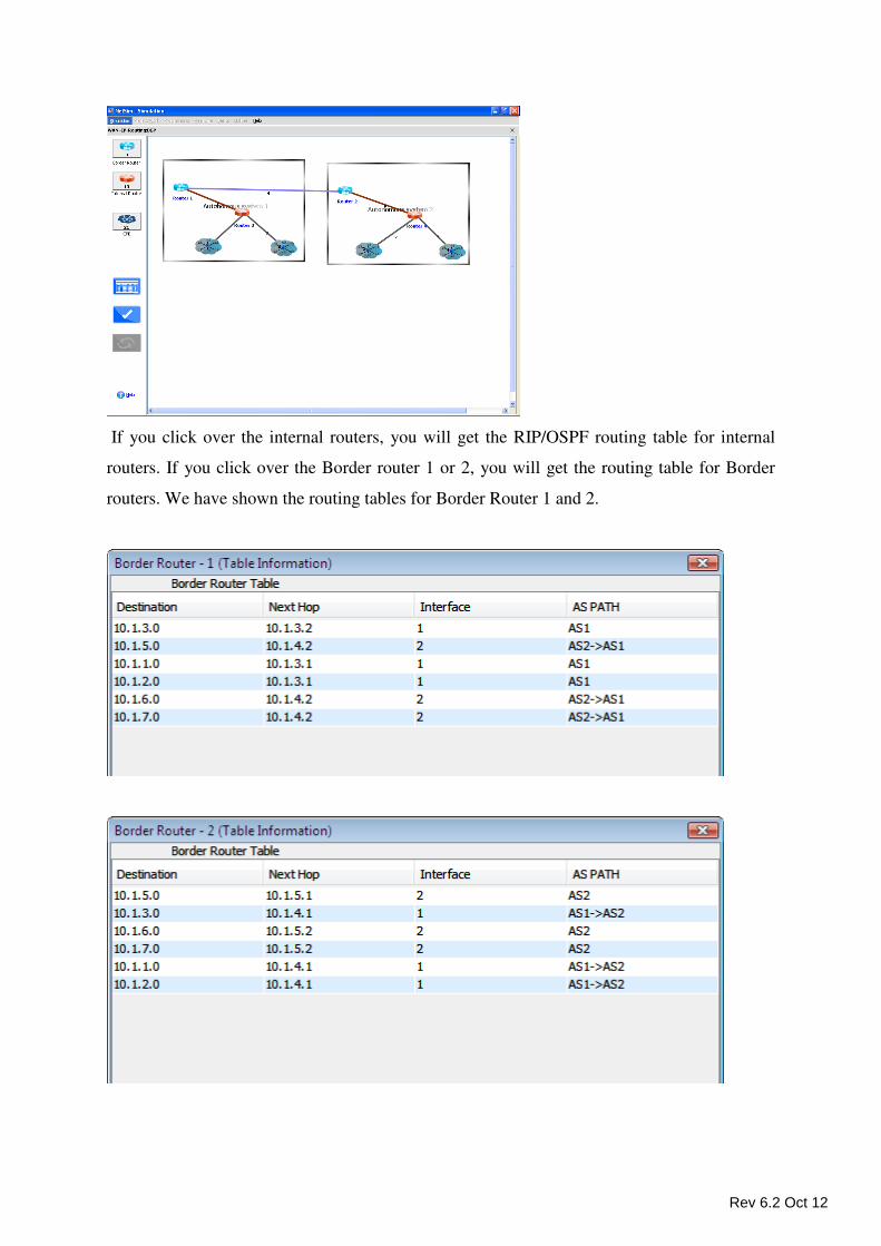
If you click over the internal routers, you will get the RIP/OSPF routing table for internal
routers. If you click over the Border router 1 or 2, you will get the routing table for Border
routers. We have shown the routing tables for Border Router 1 and 2.
Rev 6.2 Oct 12
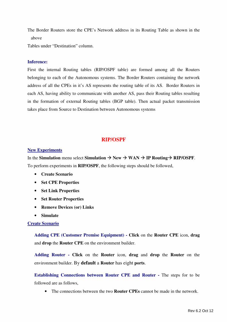
The Border Routers store the CPE’s Network address in its Routing Table as shown in the
above
Tables under “Destination” column.
Inference:
First the internal Routing tables (RIP/OSPF table) are formed among all the Routers
belonging to each of the Autonomous systems. The Border Routers containing the network
address of all the CPEs in it’s AS represents the routing table of its AS. Border Routers in
each AS, having ability to communicate with another AS, pass their Routing tables resulting
in the formation of external Routing tables (BGP table). Then actual packet transmission
takes place from Source to Destination between Autonomous systems
RIP/OSPF
New Experiments
In the Simulation menu select Simulation � New � WAN � IP Routing� RIP/OSPF.
To perform experiments in RIP/OSPF, the following steps should be followed,
• Create Scenario
• Set CPE Properties
• Set Link Properties
• Set Router Properties
• Remove Devices (or) Links
• Simulate
Create Scenario
Adding CPE (Customer Premise Equipment) - Click on the Router CPE icon, drag
and drop the Router CPE on the environment builder.
Adding Router - Click on the Router icon, drag and drop the Router on the
environment builder. By default a Router has eight ports.
Establishing Connections between Router CPE and Router - The steps for to be
followed are as follows,
• The connections between the two Router CPEs cannot be made in the network.
Rev 6.2 Oct 12
• On clicking the two devices connection can be made.
• The connection possibilities are,
o CPE to Router and
o Router to Router.
Set CPE (Customer Premises Equipment) Properties
Right Click on the appropriate node to select Properties. Inside the properties’ windows click
on Application 1 to modify its properties.
Transmission Type
This indicates the type of transmission made by this session, only Point to Point
Transmission can be made.
Destination
This property indicates the Destination CPE.
Traffic Type
This property indicates the type of traffic. The traffic can either be Voice or Data.
Voice
Codec
Codec is the component of any voice system that translates between analog speech
and the bits used to transmit them. Every codec transmits a burst of data in a packet
that can be reconstructed into voice. Five different standards of voice codec’s are
given which can be selected depending on the variations required.
Service Type
• CBR - CBR stands for Constant Bit Rate. Packets of constant size are generated
at constant inter arrival times.
• VBR - VBR stands for Variable Bit Rate. The two types of Suppression Model
that can be selected are,
• Deterministic
• Markov Chain
Click OK to accept the user entered values. Click on the close button at the top right
corner to exit the screen.
Rev 6.2 Oct 12
Data
Packet Size
Distribution: The options available for distribution are,
• Constant
• Exponential
Mean Packet Size (Bytes): Sets the size of the packets being generated by the chosen
distribution. The range of values that can be entered are between 10 to 10000 bytes.
By default 1472 bytes is entered.
Inter Arrival Time
This indicates the time gap between packets.
Distribution : The options available for distribution are,
• Constant
• Exponential
• Uniform
Mean Inter Arrival Time: Enter the average inter-arrival time between packets. A
lower inter-arrival time would lead to a higher generation rate and the vice versa. The
range of values that can be entered are between 1000 to 20000 Micro Sec. By default
20000 Micro Sec is entered.
Click OK to accept the user entered values. Click on the close button at the top right
corner to exit the screen.
Network Layer
IP Address: Set the IP Address of the Nodes by selecting the appropriate values.
Subnet Mask: Give the valid values in this field.
Priority
Click to select the Priority. Its Values ranges are Low, Normal, Medium and High. By
default the Priority is Low.
Modifying/Viewing/Accepting Properties
On opening an already configured properties of an application the input fields will be
frozen (i.e. the input cannot be changed).To modify these values click on the Modify
button in the screen. Now the input value can be changed. Click on the Accept button,
the modified values will be saved.
Rev 6.2 Oct 12
This View button is enabled once the Accept Button is clicked. To view the given
values, click on the View button.
Set Link Properties
CPE to Router Link - To set the property values right click the Link between CPE to
Router and select Properties option. There are 4 property options that are available.
They are,
Error Rate (BER) - This property defines the rate at which the data is affected by
error in the network. The values that can be selected are 10^-6, 10^-7, 10^-8, 10^-9
and No Error. By default the Error Rate is 10^-6.10^-6 means one error in every
1000000 bits transmitted.
Physical Medium - This property defines the type of Physical Medium that is used
in the network. The types of Physical Medium used in this simulation are E0, T1,
E1, T2 and E2. By default E0 is entered.
Data Rate (Mbps) - This property defines the rate at which the link transmits data.
Based on the type of Physical Medium the value of Data Rate is automatically
calculated and substituted. By default 0.064 Mbps is entered. Changes cannot be
made to this property.
Distance (Kms) - This property defines the Distance between two devices in
Kilometers. By default 1Km is entered. A 4 digit value is the maximum Distance
that can be entered.
Link Weight - This property defines the weight of the Link. This property depends
on the Protocol Type selected inside Router Properties (i.e. If the Protocol Type is
RIP then the default value is 1 and changes cannot be made. If the Protocol Type is
OSPF, then any value less than 1000 would be accepted and by default the value
entered is 1).
Router to Router Link - To change the property values right click the Link between
Router to Router and click Properties. There are 4 options for which changes can be
made. They are,
Error Rate (BER) - This property defines the rate at which the data is affected by
error in the network. The values that can be selected are 10^-6, 10^-7, 10^-8, 10^-9
Rev 6.2 Oct 12
and No Error. By default the Error Rate is 10^-6.10^-6 means one error in every
1000000 bits transmitted.
Physical Medium - This property defines the type of Physical Medium used in the
network. The Physical Medium that is used in connecting 2 Routers is a CAT5.
Data Rate (Mbps) - This property defines the rate at which the Link transmits data.
The two types of Data Rate that can be selected are, 10 and 100 Mbps. By default
10Mbps is entered.
Distance (km) - This property defines the Distance between two devices in
Kilometers. By default 1Km is entered. A 4 digit value is the maximum Distance
that can be entered.
Link Weight - This property defines the weight of the Link. This property depends
on the Protocol Type selected inside Router Properties (i.e. if the Protocol Type is
RIP then the default value is 1 and changes cannot be made. If the Protocol Type is
OSPF, then any value less than 1000 would be accepted and by default the value
entered is 1).
Set Router Properties
Router Properties - To change any property, right click on the appropriate Router to
get the option window and click Properties.
Ports Properties - The number of ports available in a Router are 8. For each Port in a
Router the following properties are available,
IP Address - The IP Address must be filled up with a valid IP Address. By default
the IP Address that would be filled is “10.1.5.1”.
Subnet Mask - By default the value that is found in the Subnet Mask field is
“255.255.255.0”.
Connected To - This property gives the Router CPE that is connected to that Port
(i.e. If the CPE1 is connected to Port1, then when Port1 is selected CPE1 would be
displayed).
Rev 6.2 Oct 12
Router Properties
Buffer Size (KB) - This property defines the Buffer size that should be selected.
Click on the drop down button to avail the values. The values that are available are,
“8, 16, 32, 64, 128, 256, 512, 1024, 2048 and 4096 (KB)”. 8KB is the default value.
Scheduling Type - Here the type of scheduler required can be selected. The 2 types
of Scheduling Type are Priority and FIFO. By default Priority is available.
Routing Protocol - The options available under Routing Protocol are,
Protocol Type - The type of protocol to be used can be selected. There are two
options for this. One is RIP and other one is OSPF.
If you select RIP as your Protocol Type, following options are available.
Periodic Time (1 to 30 sec) - The value that must be entered here should be within
the limit given. By default 30 seconds is entered.
Expiration Time (sec) - Here the value that must be entered should be greater than
that of Periodic Time and the maximum value is 180 sec. By default the value
entered is 180 seconds.
Garbage collection Time (1 to 120 sec) - Here the value that can be entered is
between 1 to 120 seconds. By default the value entered is 120 seconds.
If you select OSPF as your Protocol Type, the following options are available for you.
Router Priority (0 to 256) - Here the range of value that can be entered is 0 to 256.
By default the value entered is 256.
LSA Refresh Time (sec) - By default the value given here is 150 seconds.
LSA Max Age (sec) - By default the value given here is 300 seconds.
Data Link Layer - The options available under this property is,
Protocol Type - By default the Protocol Type found here is Ethernet. Here changes
cannot be made
Remove Devices (or) Links
Remove Link - Right click on the appropriate Link and click Remove.
Remove Router CPE - Right click on the appropriate Router CPE and click Remove.
Remove Router - Right click on the appropriate Router and click Remove.
Rev 6.2 Oct 12
Note -
• First remove the connecting Link.
• Next remove the Router / CPE. The removal of the Router / CPE can be done after the
connecting link has been removed.
Simulate - After creating the Scenario the following steps need to be followed,
• Click on Validate button.
• Click on Simulate button.
• Select the Simulation End Time and then click on “OK” button to start the
Simulation.
NetSim - Routing
Sample Experiments - User can understand the internal working of Routing through these
sample experiments. Each sample experiment covers:
• Procedure
• Sample Inputs
• Output
• Comparison chart
• Inference
Index Objective
Experiment 1
Study the working and routing table formation of Interior Routing
Protocol i.e. Routing Information protocol (RIP) and Open
Shortest Path First (OSPF)
Experiment 2
M/D/1 Queue:
I. To create an M/D/1 queue: a source to generate packets, a
queue to act as the buffer and server, a sink to dispose of
serviced packets.
II. To study how the delay of such a queuing system varies.
Experiment 3
M/M/1 Queue:
To create the queue: a source to generate packets, a queue to act as
the buffer and server, a sink to dispose of serviced packets. Study
how the delay of such a queuing system varies.
Rev 6.2 Oct 12
Sample Experiment 1
Objective:
Study the working and routing table formation of Interior routing protocols, i.e. Routing
Information Protocol (RIP) and Open Shortest Path First (OSPF).
Theory:
RIP
RIP is intended to allow hosts and gateways to exchange information for computing routes
through an IP-based network. RIP is a distance vector protocol which is based on Bellman-
Ford algorithm. This algorithm has been used for routing computation in the network.
Distance vector algorithms are based on the exchange of only a small amount of information
using RIP messages.
Each entity (router or host) that participates in the routing protocol is assumed to keep
information about all of the destinations within the system. Generally, information about all
entities connected to one network is summarized by a single entry, which describes the route
to all destinations on that network. This summarization is possible because as far as IP is
concerned, routing within a network is invisible. Each entry in this routing database includes
the next router to which datagram destined for the entity should be sent. In addition, it
includes a "metric" measuring the total distance to the entity.
Distance is a somewhat generalized concept, which may cover the time delay in getting
messages to the entity, the dollar cost of sending messages to it, etc. Distance vector
algorithms get their name from the fact that it is possible to compute optimal routes when the
only information exchanged is the list of these distances. Furthermore, information is only
exchanged among entities that are adjacent, that is, entities that share a common network.
OSPF
In OSPF, the Packets are transmitted through the shortest path between the source and
destination.
Rev 6.2 Oct 12
Shortest path:
OSPF allows administrator to assign a cost for passing through a link. The total cost of a
particular route is equal to the sum of the costs of all links that comprise the route. A router
chooses the route with the shortest (smallest) cost.
In OSPF, each router has a link state database which is tabular representation of the topology
of the network (including cost). Using Dijkstra’s algorithm each router finds the shortest path
between source and destination.
Formation of OSPF Routing Table
1. OSPF-speaking routers send Hello packets out all OSPF-enabled interfaces. If two
routers sharing a common data link agree on certain parameters specified in their
respective Hello packets, they will become neighbors.
2. Adjacencies, which can be thought of as virtual point-to-point links, are formed
between some neighbors. OSPF defines several network types and several router
types. The establishment of an adjacency is determined by the types of routers
exchanging Hellos and the type of network over which the Hellos are exchanged.
3. Each router sends link-state advertisements (LSAs) over all adjacencies. The LSAs
describe all of the router's links, or interfaces, the router's neighbors, and the state of
the links. These links might be to stub networks (networks with no other router
attached), to other OSPF routers, or to external networks (networks learned from
another routing process). Because of the varying types of link-state information,
OSPF defines multiple LSA types.
4. Each router receiving an LSA from a neighbor records the LSA in its link-state
database and sends a copy of the LSA to all of its other neighbors.
5. By flooding LSAs throughout an area, all routers will build identical link-state
databases.
6. When the databases are complete, each router uses the SPF algorithm to calculate a
loop-free graph describing the shortest (lowest cost) path to every known destination,
with itself as the root. This graph is the SPF tree.
7. Each router builds its route table from its SPF tree
Rev 6.2 Oct 12

Procedure:
How to Create Scenario:
Create Scenario: “Help � NetSim Help F1�Simulation � New �WAN � IP - Routing
� RIP/OSPF � Create Scenario”.
Sample 1:
In this Sample,
• Total no of CPE’s used: 2
• Total no of Routers used: 4
The devices are inter connected as given below,
Set the properties for each device by following the tables,
CPE Properties CPE 1
Destination CPE 2
Priority Low
Traffic Type Data
Application Data size
Distribution Constant
Application Data size (Bytes) 1472
Inter Arrival Time
Rev 6.2 Oct 12
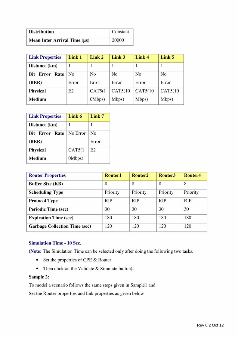
Distribution Constant
Mean Inter Arrival Time (µs) 20000
Link Properties Link 1 Link 2 Link 3 Link 4 Link 5
Distance (km) 1 1 1 1 1
Bit Error Rate
(BER)
No
Error
No
Error
No
Error
No
Error
No
Error
Physical
Medium
E2 CAT5(1
0Mbps)
CAT5(10
Mbps)
CAT5(10
Mbps)
CAT5(10
Mbps)
Link Properties Link 6 Link 7
Distance (km) 1 1
Bit Error Rate
(BER)
No Error No
Error
Physical
Medium
CAT5(1
0Mbps)
E2
Router Properties Router1 Router2 Router3 Router4
Buffer Size (KB) 8 8 8 8
Scheduling Type Priority Priority Priority Priority
Protocol Type RIP RIP RIP RIP
Periodic Time (sec) 30 30 30 30
Expiration Time (sec) 180 180 180 180
Garbage Collection Time (sec) 120 120 120 120
Simulation Time - 10 Sec.
(Note: The Simulation Time can be selected only after doing the following two tasks,
• Set the properties of CPE & Router
• Then click on the Validate & Simulate button).
Sample 2:
To model a scenario follows the same steps given in Sample1 and
Set the Router properties and link properties as given below
Rev 6.2 Oct 12
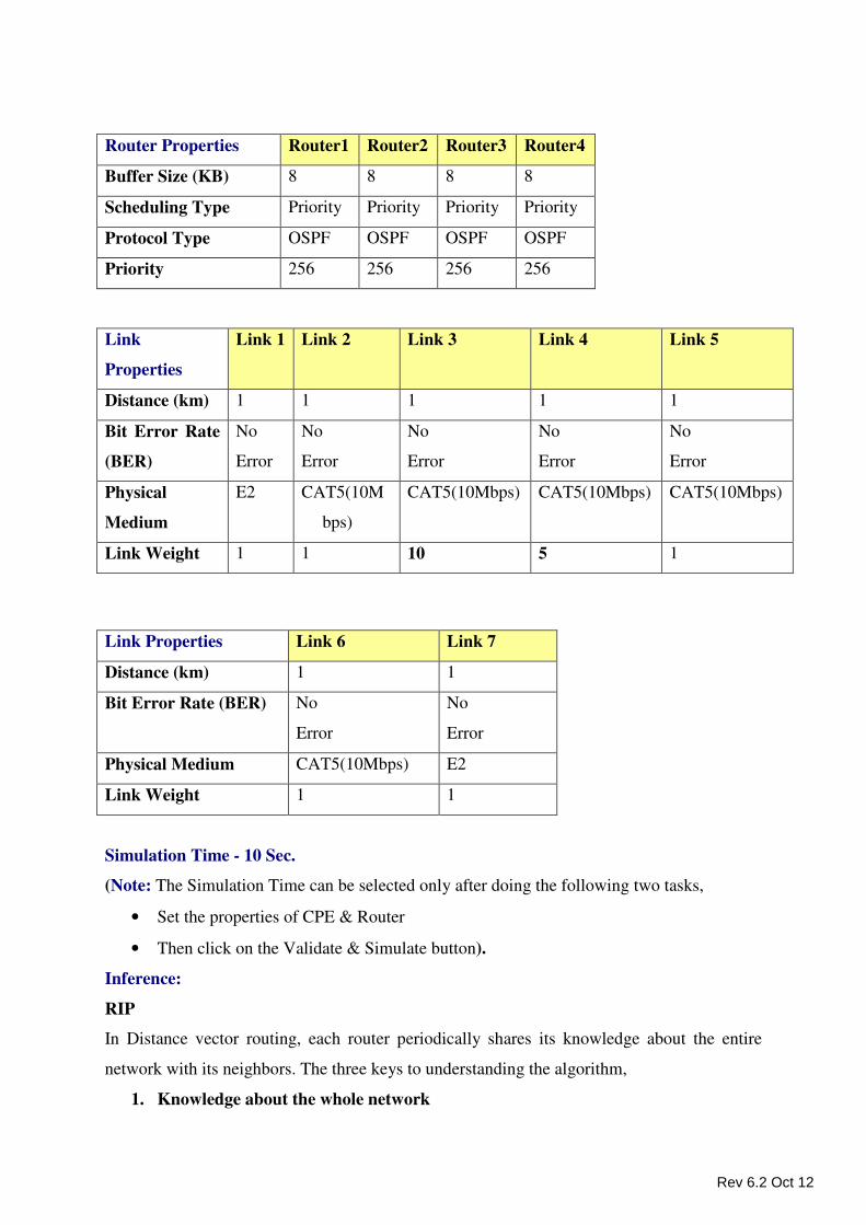
Router Properties Router1 Router2 Router3 Router4
Buffer Size (KB) 8 8 8 8
Scheduling Type Priority Priority Priority Priority
Protocol Type OSPF OSPF OSPF OSPF
Priority 256 256 256 256
Simulation Time - 10 Sec.
(Note: The Simulation Time can be selected only after doing the following two tasks,
• Set the properties of CPE & Router
• Then click on the Validate & Simulate button).
Inference:
RIP
In Distance vector routing, each router periodically shares its knowledge about the entire
network with its neighbors. The three keys to understanding the algorithm,
1. Knowledge about the whole network
Link
Properties
Link 1 Link 2 Link 3 Link 4 Link 5
Distance (km) 1 1 1 1 1
Bit Error Rate
(BER)
No
Error
No
Error
No
Error
No
Error
No
Error
Physical
Medium
E2 CAT5(10M
bps)
CAT5(10Mbps) CAT5(10Mbps) CAT5(10Mbps)
Link Weight 1 1 10 5 1
Link Properties Link 6 Link 7
Distance (km) 1 1
Bit Error Rate (BER) No
Error
No
Error
Physical Medium CAT5(10Mbps) E2
Link Weight 1 1
Rev 6.2 Oct 12
Router sends all of its collected knowledge about the network to its neighbors
2. Routing only to neighbors
Each router periodically sends its knowledge about the network only to those routers
to which it has direct links. It sends whatever knowledge it has about the whole
network through all of its ports. This information is received and kept by each
neighboring router and used to update that router’s own information about the
network.
3. Information sharing at regular intervals
For example, every 30 seconds, each router sends its information about the whole
network to its neighbors. This sharing occurs whether or not the network has changed
since the last time information was exchanged
In NetSim the Routing table Formation has 3 stages
Initial Table: This table will show the direct connections made by each Router.
Intermediate Table: The Intermediate table will have the updates of the Network in every 30
seconds
Final Table: This table is formed when there is no update in the Network.
The data should be forwarded using Routing Table with the shortest distance
The RIP table in NetSim
• After running sample1, in Network performance screen, click View Routing table
link. Then the following screen would appear
Rev 6.2 Oct 12

If you click over the routers, you will get the RIP routing table. We have shown the routing
table for Router 1
Shortest Path from CPE1 to CPE 2 in RIP. CPE 1�Router1�Router2�Router3�CPE2
Rev 6.2 Oct 12
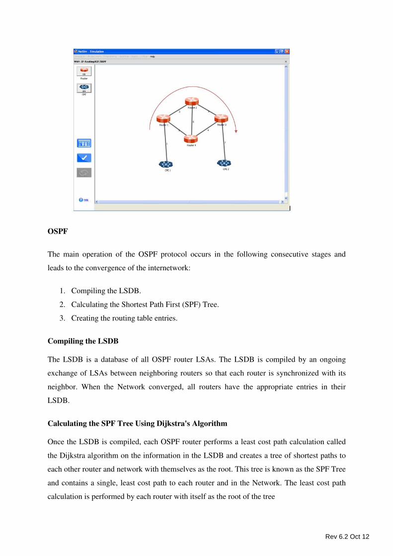
OSPF
The main operation of the OSPF protocol occurs in the following consecutive stages and
leads to the convergence of the internetwork:
1. Compiling the LSDB.
2. Calculating the Shortest Path First (SPF) Tree.
3. Creating the routing table entries.
Compiling the LSDB
The LSDB is a database of all OSPF router LSAs. The LSDB is compiled by an ongoing
exchange of LSAs between neighboring routers so that each router is synchronized with its
neighbor. When the Network converged, all routers have the appropriate entries in their
LSDB.
Calculating the SPF Tree Using Dijkstra's Algorithm
Once the LSDB is compiled, each OSPF router performs a least cost path calculation called
the Dijkstra algorithm on the information in the LSDB and creates a tree of shortest paths to
each other router and network with themselves as the root. This tree is known as the SPF Tree
and contains a single, least cost path to each router and in the Network. The least cost path
calculation is performed by each router with itself as the root of the tree
Rev 6.2 Oct 12
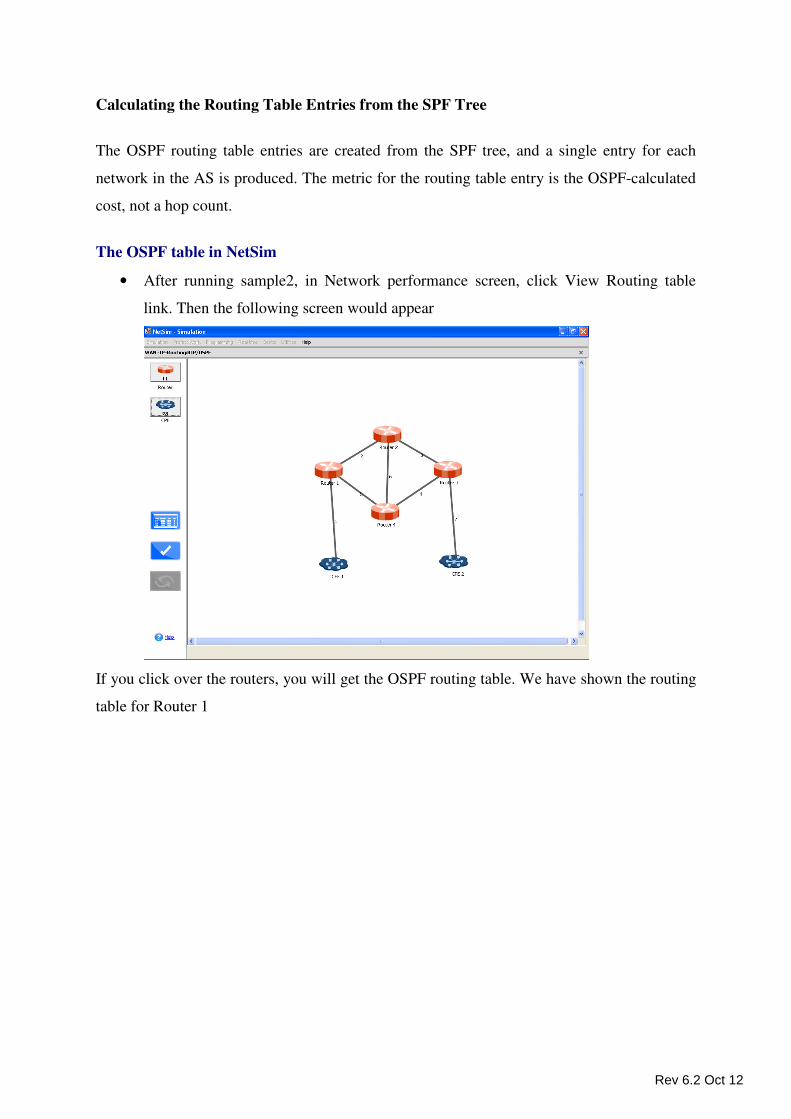
Calculating the Routing Table Entries from the SPF Tree
The OSPF routing table entries are created from the SPF tree, and a single entry for each
network in the AS is produced. The metric for the routing table entry is the OSPF-calculated
cost, not a hop count.
The OSPF table in NetSim
• After running sample2, in Network performance screen, click View Routing table
link. Then the following screen would appear
If you click over the routers, you will get the OSPF routing table. We have shown the routing
table for Router 1
Rev 6.2 Oct 12
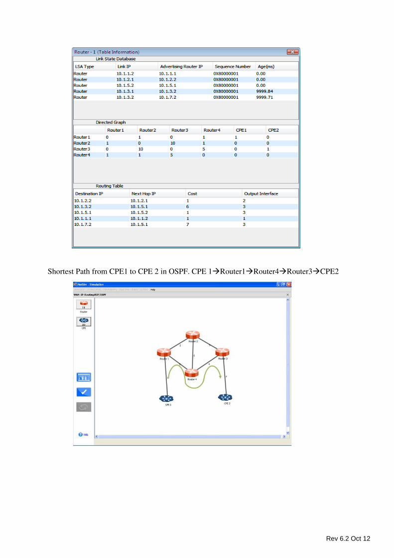
Shortest Path from CPE1 to CPE 2 in OSPF. CPE 1�Router1�Router4�Router3�CPE2
Rev 6.2 Oct 12
Sample Experiment 2
Objective:
III. To create an M/D/1 queue: a source to generate packets, a queue to act as the
buffer and server, a sink to dispose of serviced packets.
IV. To study how the delay of such a queuing system varies.
Theory:
In some systems the service time is always a constant. To approximate such a simple
systems, the M/D/1, a single-server queue model, can be used.
Following Kendall's notation it indicates a system where:
• Arrivals are a Poisson process with parameter λ;
• Service time(s) is deterministic or constant;
• There is one server.
For an M/D/1 model, the total expected waiting time (queuing time + service time) is
Where, ρ is the utilization given as follows, The above formula can also be written as
follows,
Where, µ = Service Rate = 1/Service time
To model an M/D/1 system in NetSim, we use the following model
Rev 6.2 Oct 12
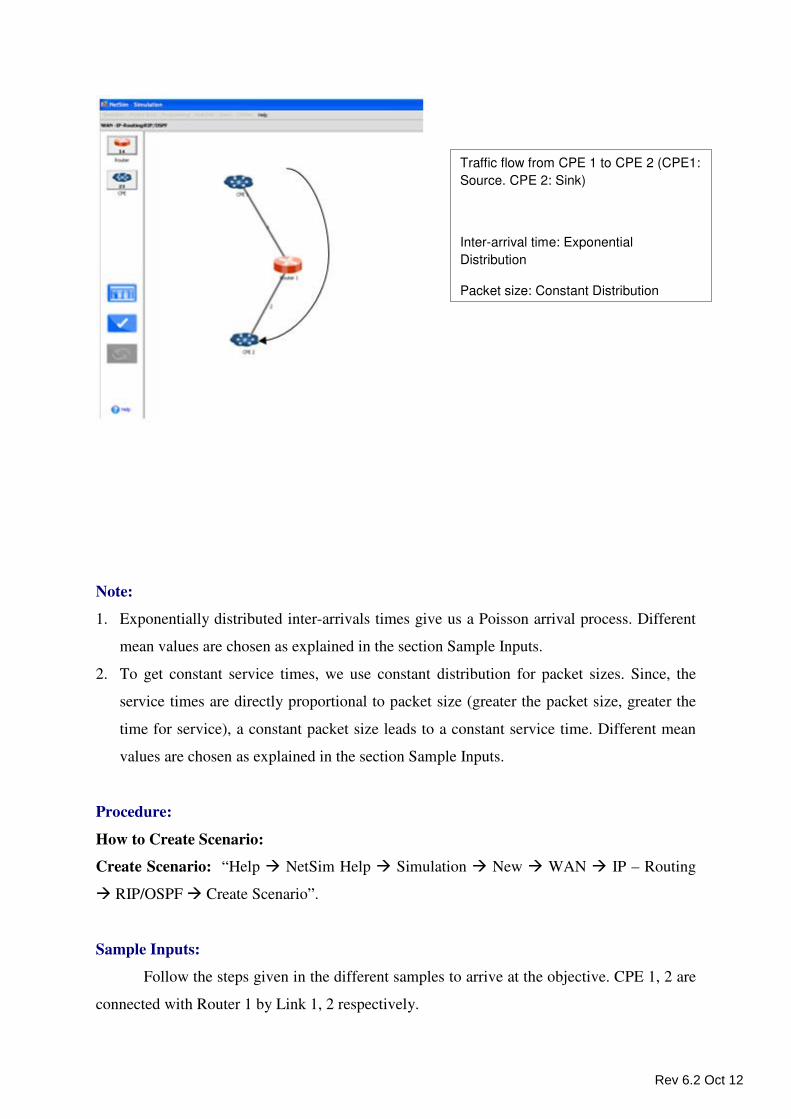
Note:
1. Exponentially distributed inter-arrivals times give us a Poisson arrival process. Different
mean values are chosen as explained in the section Sample Inputs.
2. To get constant service times, we use constant distribution for packet sizes. Since, the
service times are directly proportional to packet size (greater the packet size, greater the
time for service), a constant packet size leads to a constant service time. Different mean
values are chosen as explained in the section Sample Inputs.
Procedure:
How to Create Scenario:
Create Scenario: “Help � NetSim Help � Simulation � New � WAN � IP – Routing
� RIP/OSPF � Create Scenario”.
Sample Inputs:
Follow the steps given in the different samples to arrive at the objective. CPE 1, 2 are
connected with Router 1 by Link 1, 2 respectively.
Traffic flow from CPE 1 to CPE 2 (CPE1:
Source. CPE 2: Sink)
Inter-arrival time: Exponential
Distribution
Packet size: Constant Distribution
Rev 6.2 Oct 12
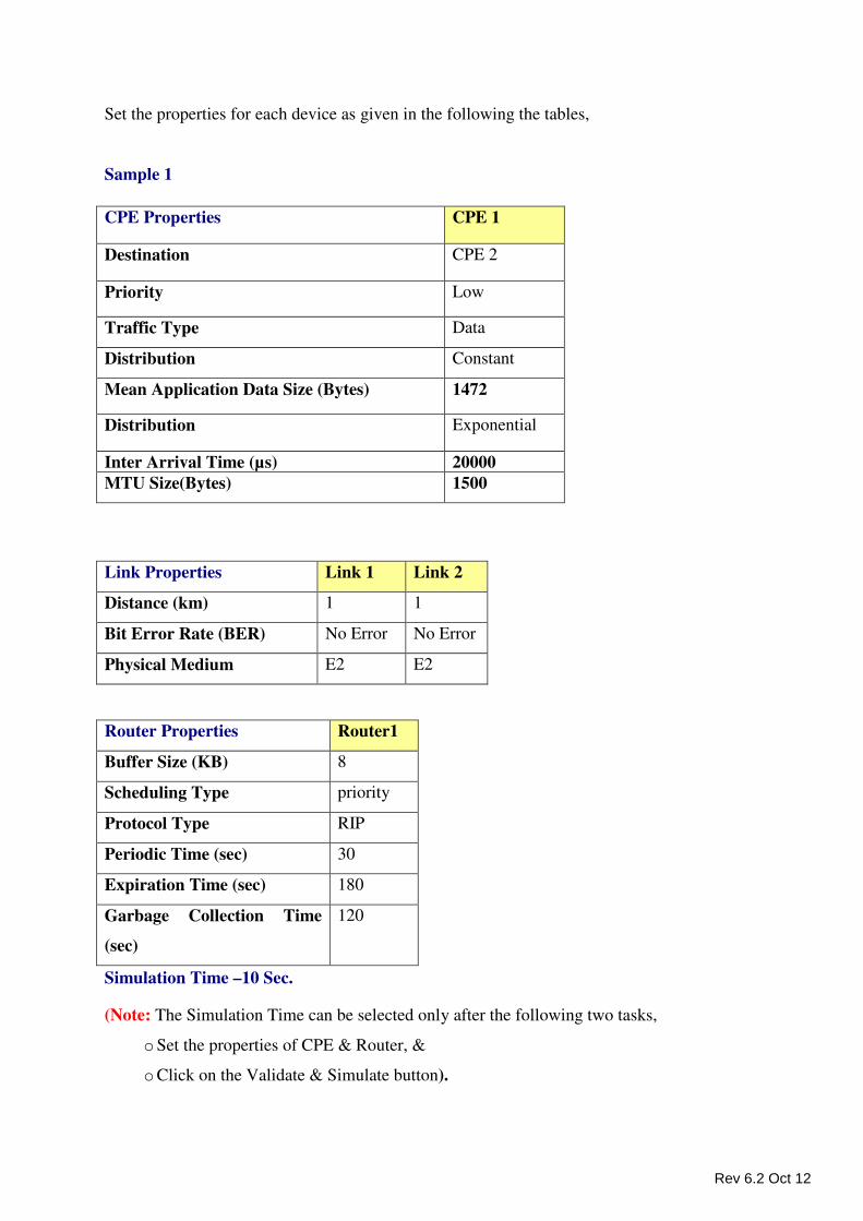
Set the properties for each device as given in the following the tables,
Sample 1
Simulation Time –10 Sec.
(Note: The Simulation Time can be selected only after the following two tasks,
o Set the properties of CPE & Router, &
o Click on the Validate & Simulate button).
CPE Properties CPE 1
Destination CPE 2
Priority Low
Traffic Type Data
Distribution Constant
Mean Application Data Size (Bytes) 1472
Distribution Exponential
Inter Arrival Time (µs) 20000
MTU Size(Bytes) 1500
Link Properties Link 1 Link 2
Distance (km) 1 1
Bit Error Rate (BER) No Error No Error
Physical Medium E2 E2
Router Properties Router1
Buffer Size (KB) 8
Scheduling Type priority
Protocol Type RIP
Periodic Time (sec) 30
Expiration Time (sec) 180
Garbage Collection Time
(sec)
120
Rev 6.2 Oct 12
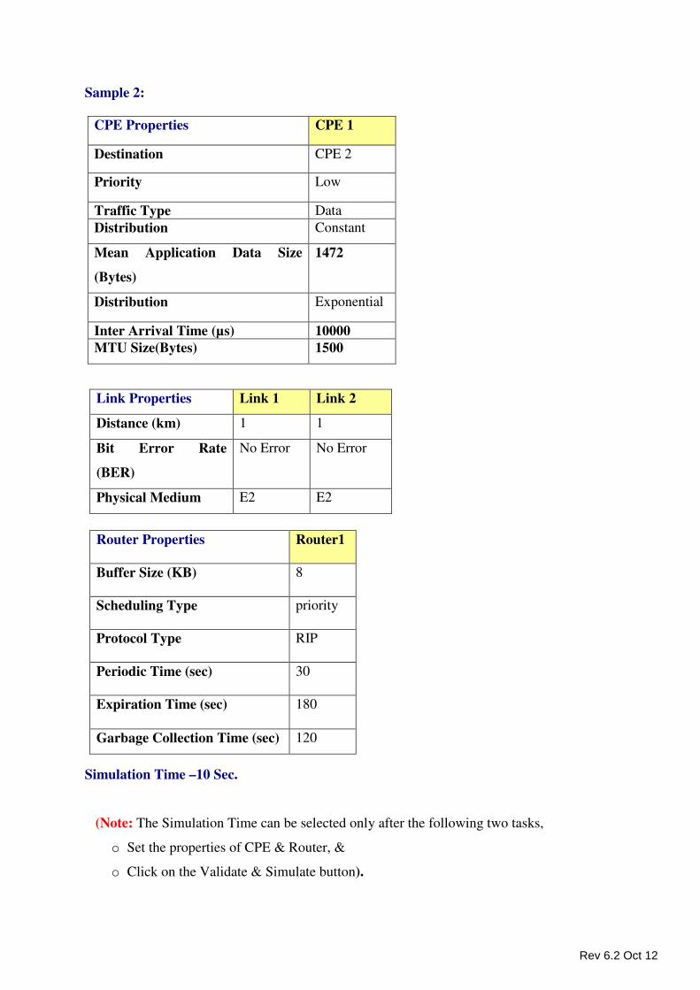
Sample 2:
Simulation Time –10 Sec.
(Note: The Simulation Time can be selected only after the following two tasks,
o Set the properties of CPE & Router, &
o Click on the Validate & Simulate button).
CPE Properties CPE 1
Destination CPE 2
Priority Low
Traffic Type Data
Distribution Constant
Mean Application Data Size
(Bytes)
1472
Distribution Exponential
Inter Arrival Time (µs) 10000
MTU Size(Bytes) 1500
Link Properties Link 1 Link 2
Distance (km) 1 1
Bit Error Rate
(BER)
No Error No Error
Physical Medium E2 E2
Router Properties Router1
Buffer Size (KB) 8
Scheduling Type priority
Protocol Type RIP
Periodic Time (sec) 30
Expiration Time (sec) 180
Garbage Collection Time (sec) 120
Rev 6.2 Oct 12
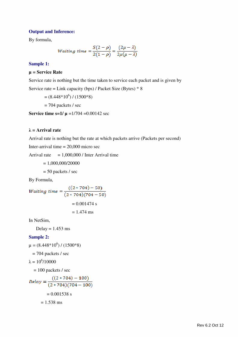
Output and Inference:
By formula,
Sample 1:
µ = Service Rate
Service rate is nothing but the time taken to service each packet and is given by
Service rate = Link capacity (bps) / Packet Size (Bytes) * 8
= (8.448*106) / (1500*8)
= 704 packets / sec
Service time s=1/ µ =1/704 =0.00142 sec
λ = Arrival rate
Arrival rate is nothing but the rate at which packets arrive (Packets per second)
Inter-arrival time = 20,000 micro sec
Arrival rate = 1,000,000 / Inter Arrival time
= 1,000,000/20000
= 50 packets / sec
By Formula,
= 0.001474 s
= 1.474 ms
In NetSim,
Delay = 1.453 ms
Sample 2:
µ = (8.448*106) / (1500*8)
= 704 packets / sec
λ = 106/10000
= 100 packets / sec
= 0.001538 s
= 1.538 ms
Rev 6.2 Oct 12
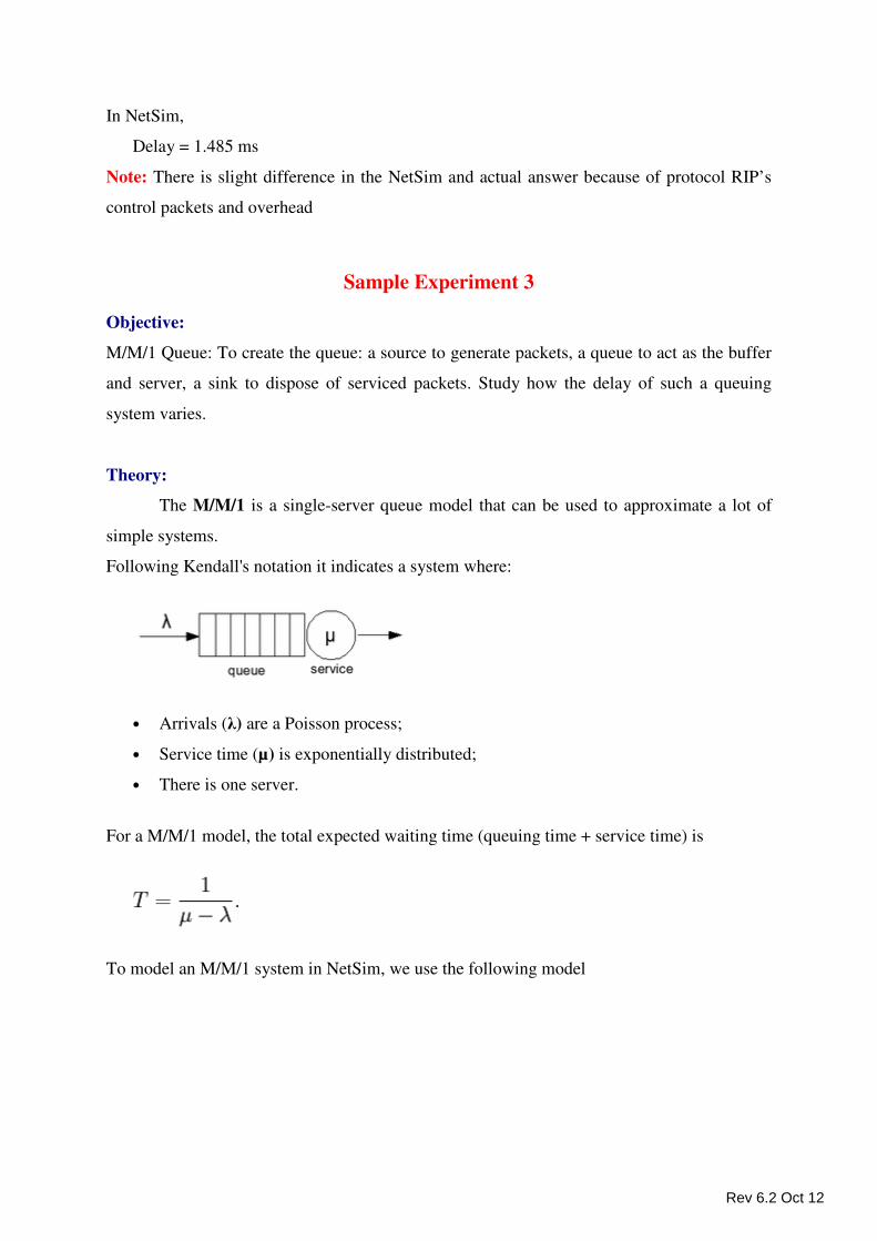
In NetSim,
Delay = 1.485 ms
Note: There is slight difference in the NetSim and actual answer because of protocol RIP’s
control packets and overhead
Sample Experiment 3
Objective:
M/M/1 Queue: To create the queue: a source to generate packets, a queue to act as the buffer
and server, a sink to dispose of serviced packets. Study how the delay of such a queuing
system varies.
Theory:
The M/M/1 is a single-server queue model that can be used to approximate a lot of
simple systems.
Following Kendall's notation it indicates a system where:
• Arrivals (λ) are a Poisson process;
• Service time (µ) is exponentially distributed;
• There is one server.
For a M/M/1 model, the total expected waiting time (queuing time + service time) is
To model an M/M/1 system in NetSim, we use the following model
Rev 6.2 Oct 12
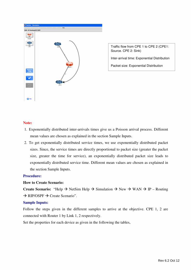
Note:
1. Exponentially distributed inter-arrivals times give us a Poisson arrival process. Different
mean values are chosen as explained in the section Sample Inputs.
2. To get exponentially distributed service times, we use exponentially distributed packet
sizes. Since, the service times are directly proportional to packet size (greater the packet
size, greater the time for service), an exponentially distributed packet size leads to
exponentially distributed service time. Different mean values are chosen as explained in
the section Sample Inputs.
Procedure:
How to Create Scenario:
Create Scenario: “Help � NetSim Help � Simulation � New � WAN � IP – Routing
� RIP/OSPF � Create Scenario”.
Sample Inputs:
Follow the steps given in the different samples to arrive at the objective. CPE 1, 2 are
connected with Router 1 by Link 1, 2 respectively.
Set the properties for each device as given in the following the tables,
Traffic flow from CPE 1 to CPE 2 (CPE1:
Source. CPE 2: Sink)
Inter-arrival time: Exponential Distribution
Packet size: Exponential Distribution
Rev 6.2 Oct 12
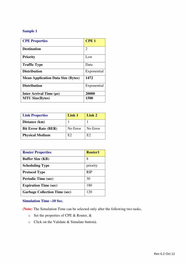
Sample 1
Simulation Time –10 Sec.
(Note: The Simulation Time can be selected only after the following two tasks,
o Set the properties of CPE & Router, &
o Click on the Validate & Simulate button).
CPE Properties CPE 1
Destination 2
Priority Low
Traffic Type Data
Distribution Exponential
Mean Application Data Size (Bytes) 1472
Distribution Exponential
Inter Arrival Time (µs) 20000
MTU Size(Bytes) 1500
Link Properties Link 1 Link 2
Distance (km) 1 1
Bit Error Rate (BER) No Error No Error
Physical Medium E2 E2
Router Properties Router1
Buffer Size (KB) 8
Scheduling Type priority
Protocol Type RIP
Periodic Time (sec) 30
Expiration Time (sec) 180
Garbage Collection Time (sec) 120
Rev 6.2 Oct 12
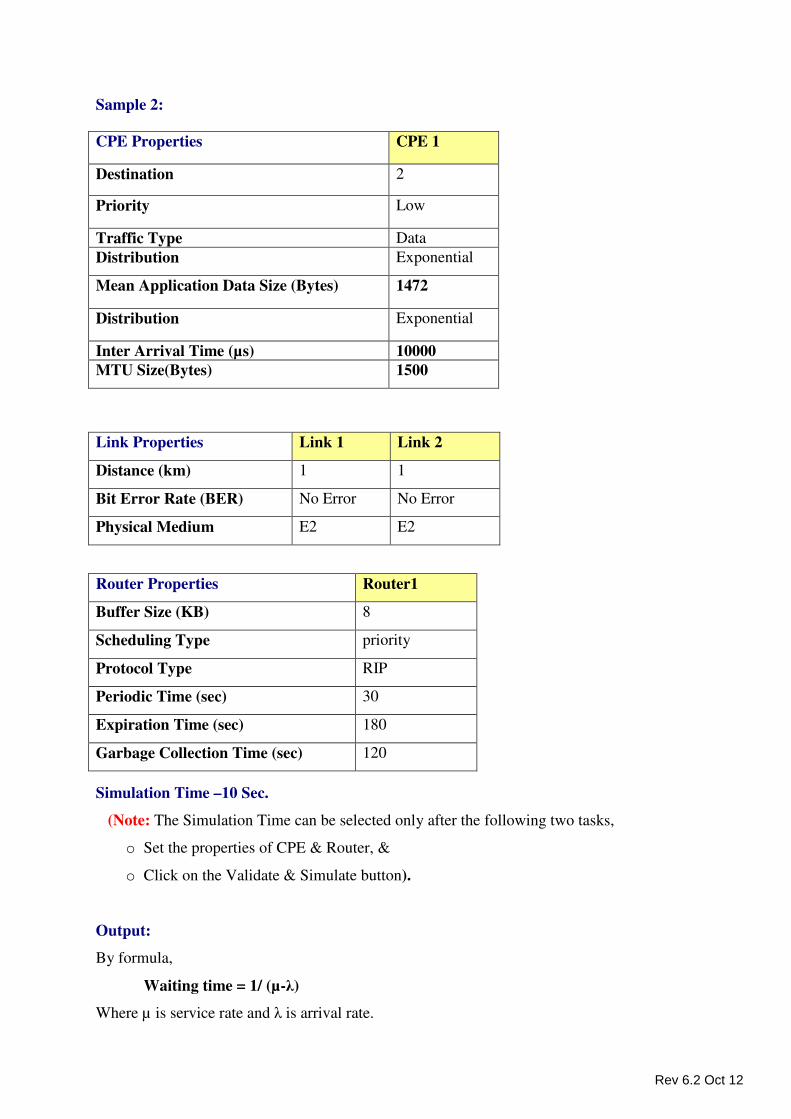
Sample 2:
Simulation Time –10 Sec.
(Note: The Simulation Time can be selected only after the following two tasks,
o Set the properties of CPE & Router, &
o Click on the Validate & Simulate button).
Output:
By formula,
Waiting time = 1/ (µ-λ)
Where µ is service rate and λ is arrival rate.
CPE Properties CPE 1
Destination 2
Priority Low
Traffic Type Data
Distribution Exponential
Mean Application Data Size (Bytes) 1472
Distribution Exponential
Inter Arrival Time (µs) 10000
MTU Size(Bytes) 1500
Link Properties Link 1 Link 2
Distance (km) 1 1
Bit Error Rate (BER) No Error No Error
Physical Medium E2 E2
Router Properties Router1
Buffer Size (KB) 8
Scheduling Type priority
Protocol Type RIP
Periodic Time (sec) 30
Expiration Time (sec) 180
Garbage Collection Time (sec) 120
Rev 6.2 Oct 12
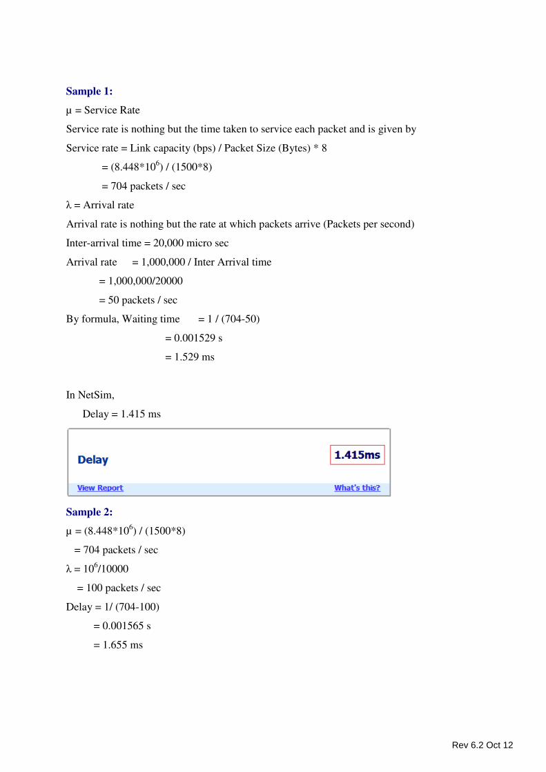
Sample 1:
µ = Service Rate
Service rate is nothing but the time taken to service each packet and is given by
Service rate = Link capacity (bps) / Packet Size (Bytes) * 8
= (8.448*106) / (1500*8)
= 704 packets / sec
λ = Arrival rate
Arrival rate is nothing but the rate at which packets arrive (Packets per second)
Inter-arrival time = 20,000 micro sec
Arrival rate = 1,000,000 / Inter Arrival time
= 1,000,000/20000
= 50 packets / sec
By formula, Waiting time = 1 / (704-50)
= 0.001529 s
= 1.529 ms
In NetSim,
Delay = 1.415 ms
Sample 2:
µ = (8.448*106) / (1500*8)
= 704 packets / sec
λ = 106/10000
= 100 packets / sec
Delay = 1/ (704-100)
= 0.001565 s
= 1.655 ms
Rev 6.2 Oct 12
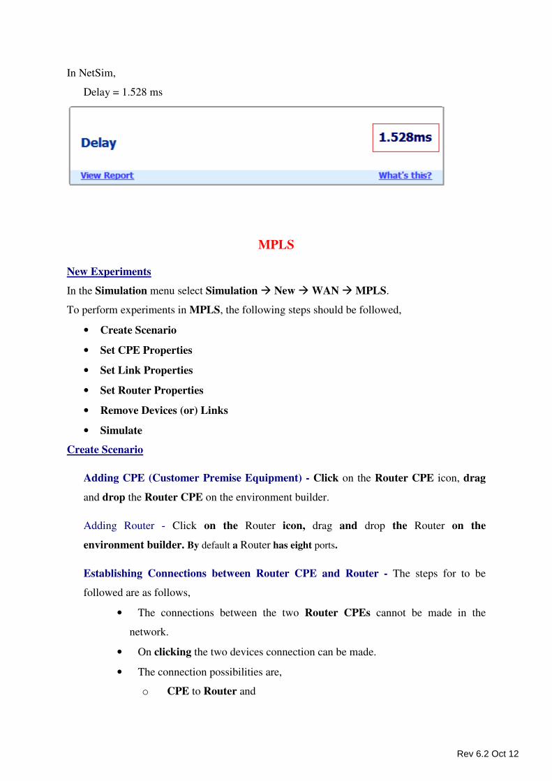
In NetSim,
Delay = 1.528 ms
MPLS
New Experiments
In the Simulation menu select Simulation � New � WAN � MPLS.
To perform experiments in MPLS, the following steps should be followed,
• Create Scenario
• Set CPE Properties
• Set Link Properties
• Set Router Properties
• Remove Devices (or) Links
• Simulate
Create Scenario
Adding CPE (Customer Premise Equipment) - Click on the Router CPE icon, drag
and drop the Router CPE on the environment builder.
Adding Router - Click on the Router icon, drag and drop the Router on the
environment builder. By default a Router has eight ports.
Establishing Connections between Router CPE and Router - The steps for to be
followed are as follows,
• The connections between the two Router CPEs cannot be made in the
network.
• On clicking the two devices connection can be made.
• The connection possibilities are,
o CPE to Router and
Rev 6.2 Oct 12
o Router to Router.
Set CPE (Customer Premises Equipment) Properties
Right Click on the appropriate node to select Properties. Inside the properties’ windows click
on Application 1 to modify its properties.
Transmission Type
This indicates the type of transmission made by this session, only Point to Point
Transmission can be made.
Destination
This property indicates the Destination CPE.
Traffic Type
This property indicates the type of traffic. The traffic can either be Voice or Data.
Voice
Codec
Codec is the component of any voice system that translates between analog speech and
the bits used to transmit them. Every codec transmits a burst of data in a packet that can
be reconstructed into voice. Six different standards of voice codec’s are given which can
be selected depending on the variations required.
Service Type
• CBR - CBR stands for Constant Bit Rate. Packets of constant size are generated at
constant inter arrival times.
Click OK to accept the user entered values. Click on the close button at the top right
corner to exit the screen.
Data
Packet Size
Distribution: The options available for distribution are,
• Constant
Mean Packet Size (Bytes): Sets the size of the packets being generated by the
Constant distribution. The value of mean packet size is 1472 bytes
Inter Arrival Time
This indicates the time gap between packets.
Rev 6.2 Oct 12
Reserved Bandwidth:
This indicates the bandwidth reserved by user. The range of value is between 0.6 Mbps
and 11 Mbps
Click OK to accept the user entered values. Click on the close button at the top right
corner to exit the screen.
Network Layer
IP Address: Set the IP Address of the Nodes by selecting the appropriate values.
Subnet Mask: Give the valid values in this field.
Priority
Click to select the Priority. Its Values ranges from Low, Normal, Medium, and High.
By default the Priority is Low.
Modifying/Viewing/Accepting Properties
On opening an already configured properties of an application the input fields will be
frozen (i.e. the input cannot be changed).To modify these values click on the Modify
button in the screen. Now the input value can be changed. Click on the Accept button,
the modified values will be saved.
This View button is enabled once the Accept Button is clicked. To view the given
values, click on the View button.
Set Link Properties
Link Properties
CPE to Router Link - To set the property values right click the Link between CPE to
Router and select Properties option. There are 4 property options that are available.
They are,
Error Rate (BER) - This property defines the rate at which the data is affected by error
in the network. The values that can be selected are 10^-6, 10^-7, 10^-8, 10^-9 and No
Error. By default the Error Rate is 10^-6.10^-6 means one error in every 1000000 bits
transmitted.
Physical Medium - This property defines the type of Physical Medium that is used in
the network. The types of Physical Medium used in this simulation are E0, T1, E1, T2
and E2. By default E0 is entered.
Rev 6.2 Oct 12
Data Rate (Mbps) - This property defines the rate at which the link transmits data. Based
on the type of Physical Medium the value of Data Rate is automatically calculated and
substituted. By default 0.064 Mbps is entered. Changes cannot be made to this property.
Distance (Kms) - This property defines the Distance between two devices in
Kilometers. By default 1Km is entered. A 4 digit value is the maximum Distance
that can be entered.
Link Weight - This property defines the weight of the Link. This property depends
on the Protocol Type selected inside Router Properties (i.e. If the Protocol Type is
RIP then the default value is 1 and changes cannot be made. If the Protocol Type is
OSPF, then any value less than 1000 would be accepted and by default the value
entered is 1).
Router to Router Link - To change the property values right click the Link between
Router to Router and click Properties. There are 4 options for which changes can be
made. They are,
Error Rate (BER) - This property defines the rate at which the data is affected by
error in the network. The values that can be selected are 10^-6, 10^-7, 10^-8, 10^-9
and No Error. By default the Error Rate is 10^-6.10^-6 means one error in every
1000000 bits transmitted.
Physical Medium - This property defines the type of Physical Medium used in the
network. The Physical Medium that is used in connecting 2 Routers is a CAT5.
Data Rate (Mbps) - This property defines the rate at which the Link transmits data.
The two types of Data Rate that can be selected are, 10 and 100 Mbps. By default
10Mbps is entered.
Distance (km) - This property defines the Distance between two devices in
Kilometers. By default 1Km is entered. A 4 digit value is the maximum Distance
that can be entered.
Link Weight - This property defines the weight of the Link. This property depends
on the Protocol Type selected inside Router Properties (i.e. if the Protocol Type is
RIP then the default value is 1 and changes cannot be made. If the Protocol Type is
OSPF, then any value less than 1000 would be accepted and by default the value
entered is 1).
Rev 6.2 Oct 12
Set Router Properties
Router Properties - To change any property, right click on the appropriate Router to
get the option window and click Properties.
Ports Properties - The number of ports available in a Router are 8. For each Port in a
Router the following properties are available,
Ip Address - The Ip Address must be filled up with a valid Ip Address. By default
the Ip Address that would be filled is “10.1.5.1”.
Subnet Mask - By default the value that is found in the Subnet Mask field is
“255.255.255.0”.
Connected To - This property gives the Router CPE that is connected to that Port
(i.e. If the CPE1 is connected to Port1, then when Port1 is selected CPE1 would be
displayed).
Router Properties
Buffer Size (KB) - This property defines the Buffer size that should be selected.
Click on the drop down button to avail the values. The values that are available are,
“8, 16, 32, 64, 128, 256, 512, 1024, 2048 and 4096 (KB)”. 8KB is the default value.
Scheduling Type - Here the type of scheduler required can be selected. The 2 types
of Scheduling Type are Priority and FIFO. By default Priority is available.
Routing Protocol - The options available under Routing Protocol are,
Protocol Type - The type of protocol to be used can be selected.
Router Priority – This indicates the priority of router. Range of the value is between
0 and 256
LSA Refresh time (sec) – The refresh time for LSA for the simulation is 150 s
LSA Max Age (sec) - The Max Age of LSA for the simulation is 350 s
Rev 6.2 Oct 12
MPLS Properties
Traffic Engineering – Here the traffic engineering can be selected or deselected
Protocol type – Based on the selection and de selection of traffic engineering, the
protocol type will be displayed. If the traffic engineering is selected, the protocol type is
CR-LDP. Otherwise, the protocol type is LDP
Label Distribution type – Label Distribution type is Downstream on Demand
Label Distribution mode – Label Distribution mode is Ordered
Label Retention type – Label Retention type is Conservative
Data Link Layer - The options available under this property is,
Protocol Type - By default the Protocol Type found here is Ethernet. Here changes
cannot be made.
MAC Address – MAC address of router is displayed
Remove Devices (or) Links
Remove Link - Right click on the appropriate Link and click Remove.
Remove Router CPE - Right click on the appropriate Router CPE and click
Remove.
Remove Router - Right click on the appropriate Router and click Remove.
Note -
• First remove the connecting Link.
• Next remove the Router / CPE. The removal of the Router / CPE can be done
after the connecting link has been removed.
Simulate - After creating the Scenario the following steps need to be followed,
• Click on Validate button.
• Click on Simulate button.
• Select the Simulation End Time and then click on “OK” button to start the
Simulation.
Rev 6.2 Oct 12
NetSim - MPLS
Sample Experiments - User can understand the internal working of MPLS through these
sample experiments. Each sample experiment covers:
• Procedure
• Sample Inputs
• Output
• Comparison chart
• Inference
Index Objective
Experiment 1 Study how the LSP varies for different traffic in MPLS -TE
(Traffic Engineering)
Sample Experiment
Objective:
Study how the LSP varies for different traffic in MPLS -TE (Traffic Engineering)
Theory:
Traffic Engineering is the process of controlling how traffic flows through one’s network so
as to optimize resource utilization and network performance. Traffic Engineering is needed in
the Internet mainly because current IGPs (Interior Gateway Protocols – RIP, OSPF) always
use the shortest paths to forward all traffics. But MPLS with traffic engineering use different
paths to forward different traffics.
Procedure:
How to Create Scenario:
o Create Scenario: “Help � Simulation � New � WAN � MPLS� Create
Scenario”.
Sample Inputs:
Follow the steps given in the different samples to arrive at the objective.
Rev 6.2 Oct 12
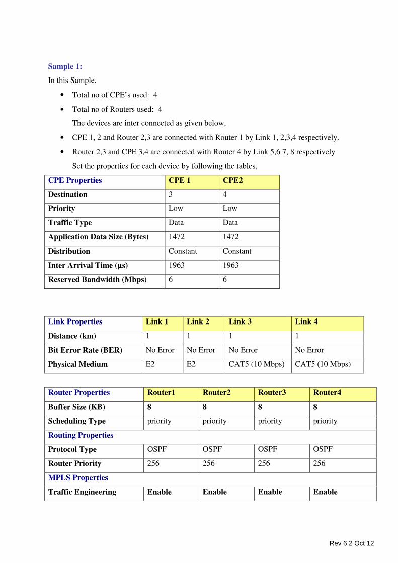
Sample 1:
In this Sample,
• Total no of CPE’s used: 4
• Total no of Routers used: 4
The devices are inter connected as given below,
• CPE 1, 2 and Router 2,3 are connected with Router 1 by Link 1, 2,3,4 respectively.
• Router 2,3 and CPE 3,4 are connected with Router 4 by Link 5,6 7, 8 respectively
Set the properties for each device by following the tables,
CPE Properties CPE 1 CPE2
Destination 3 4
Priority Low Low
Traffic Type Data Data
Application Data Size (Bytes) 1472 1472
Distribution Constant Constant
Inter Arrival Time (µs) 1963 1963
Reserved Bandwidth (Mbps) 6 6
Link Properties Link 1 Link 2 Link 3 Link 4
Distance (km) 1 1 1 1
Bit Error Rate (BER) No Error No Error No Error No Error
Physical Medium E2 E2 CAT5 (10 Mbps) CAT5 (10 Mbps)
Router Properties Router1 Router2 Router3 Router4
Buffer Size (KB) 8 8 8 8
Scheduling Type priority priority priority priority
Routing Properties
Protocol Type OSPF OSPF OSPF OSPF
Router Priority 256 256 256 256
MPLS Properties
Traffic Engineering Enable Enable Enable Enable
Rev 6.2 Oct 12
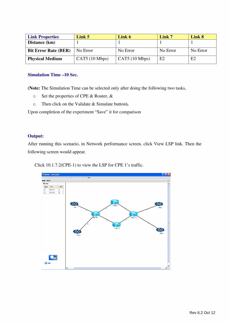
Simulation Time –10 Sec.
(Note: The Simulation Time can be selected only after doing the following two tasks,
o Set the properties of CPE & Router, &
o Then click on the Validate & Simulate button).
Upon completion of the experiment “Save” it for comparison
Output:
After running this scenario, in Network performance screen, click View LSP link. Then the
following screen would appear.
Click 10.1.7.2(CPE-1) to view the LSP for CPE 1’s traffic.
Link Properties Link 5 Link 6 Link 7 Link 8
Distance (km) 1 1 1 1
Bit Error Rate (BER) No Error No Error No Error No Error
Physical Medium CAT5 (10 Mbps) CAT5 (10 Mbps) E2 E2
Rev 6.2 Oct 12
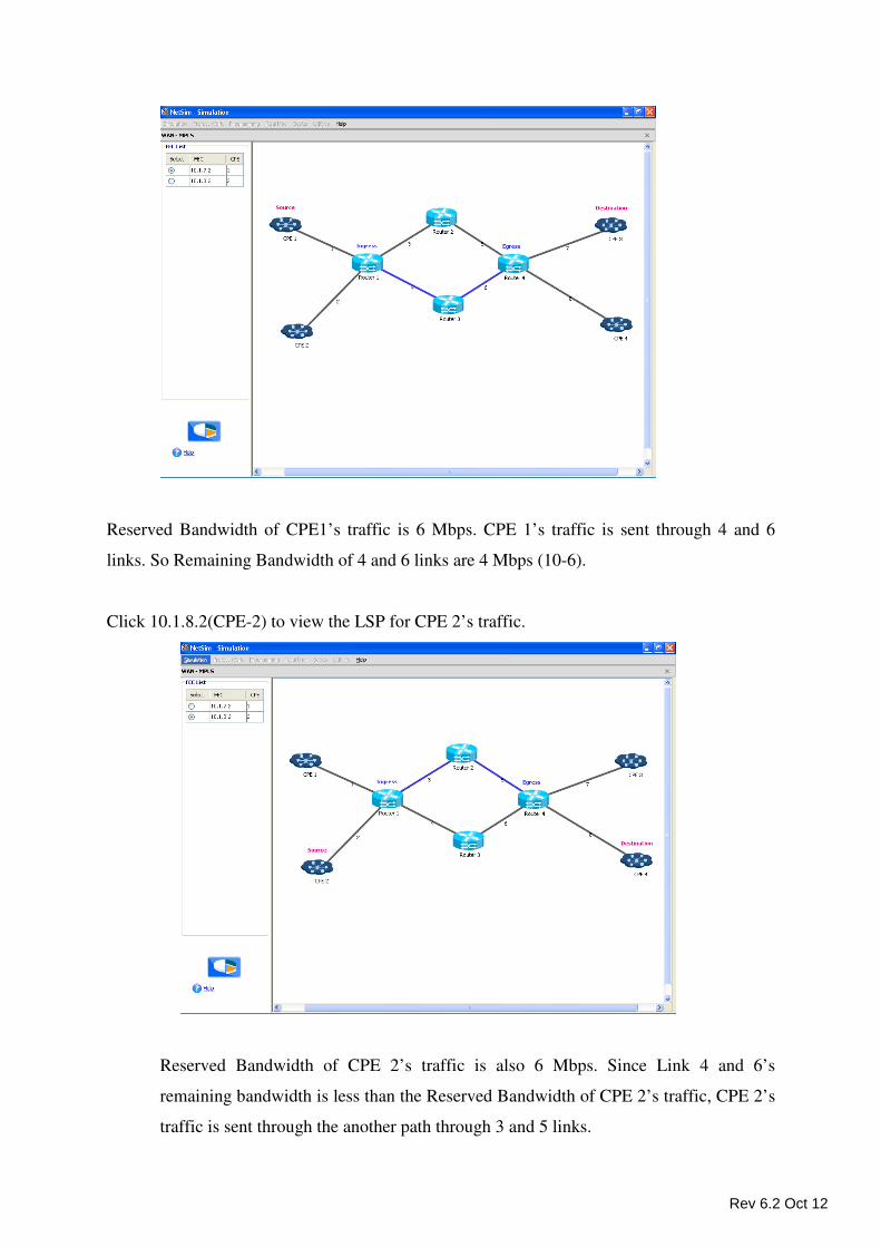
Reserved Bandwidth of CPE1’s traffic is 6 Mbps. CPE 1’s traffic is sent through 4 and 6
links. So Remaining Bandwidth of 4 and 6 links are 4 Mbps (10-6).
Click 10.1.8.2(CPE-2) to view the LSP for CPE 2’s traffic.
Reserved Bandwidth of CPE 2’s traffic is also 6 Mbps. Since Link 4 and 6’s
remaining bandwidth is less than the Reserved Bandwidth of CPE 2’s traffic, CPE 2’s
traffic is sent through the another path through 3 and 5 links.
Rev 6.2 Oct 12
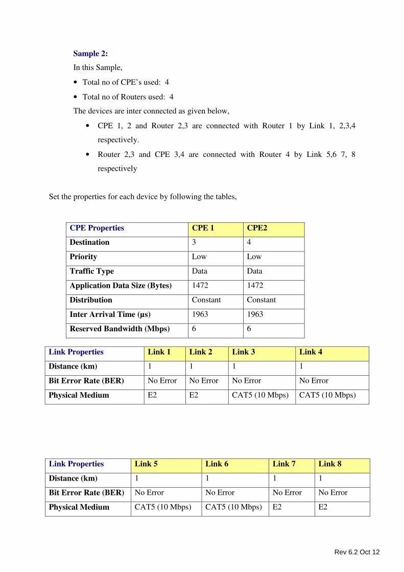
Sample 2:
In this Sample,
• Total no of CPE’s used: 4
• Total no of Routers used: 4
The devices are inter connected as given below,
• CPE 1, 2 and Router 2,3 are connected with Router 1 by Link 1, 2,3,4
respectively.
• Router 2,3 and CPE 3,4 are connected with Router 4 by Link 5,6 7, 8
respectively
Set the properties for each device by following the tables,
Link Properties Link 1 Link 2 Link 3 Link 4
Distance (km) 1 1 1 1
Bit Error Rate (BER) No Error No Error No Error No Error
Physical Medium E2 E2 CAT5 (10 Mbps) CAT5 (10 Mbps)
CPE Properties CPE 1 CPE2
Destination 3 4
Priority Low Low
Traffic Type Data Data
Application Data Size (Bytes) 1472 1472
Distribution Constant Constant
Inter Arrival Time (µs) 1963 1963
Reserved Bandwidth (Mbps) 6 6
Link Properties Link 5 Link 6 Link 7 Link 8
Distance (km) 1 1 1 1
Bit Error Rate (BER) No Error No Error No Error No Error
Physical Medium CAT5 (10 Mbps) CAT5 (10 Mbps) E2 E2
Rev 6.2 Oct 12
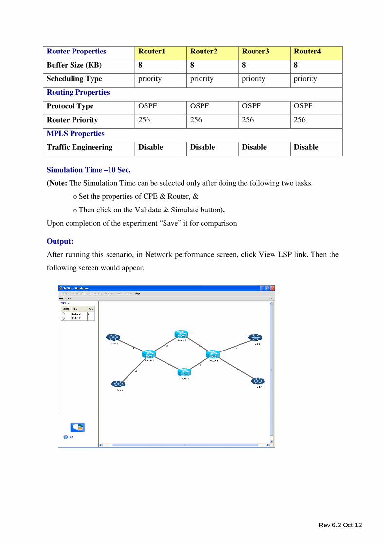
Router Properties Router1 Router2 Router3 Router4
Buffer Size (KB) 8 8 8 8
Scheduling Type priority priority priority priority
Routing Properties
Protocol Type OSPF OSPF OSPF OSPF
Router Priority 256 256 256 256
MPLS Properties
Traffic Engineering Disable Disable Disable Disable
Simulation Time –10 Sec.
(Note: The Simulation Time can be selected only after doing the following two tasks,
o Set the properties of CPE & Router, &
o Then click on the Validate & Simulate button).
Upon completion of the experiment “Save” it for comparison
Output:
After running this scenario, in Network performance screen, click View LSP link. Then the
following screen would appear.
Rev 6.2 Oct 12
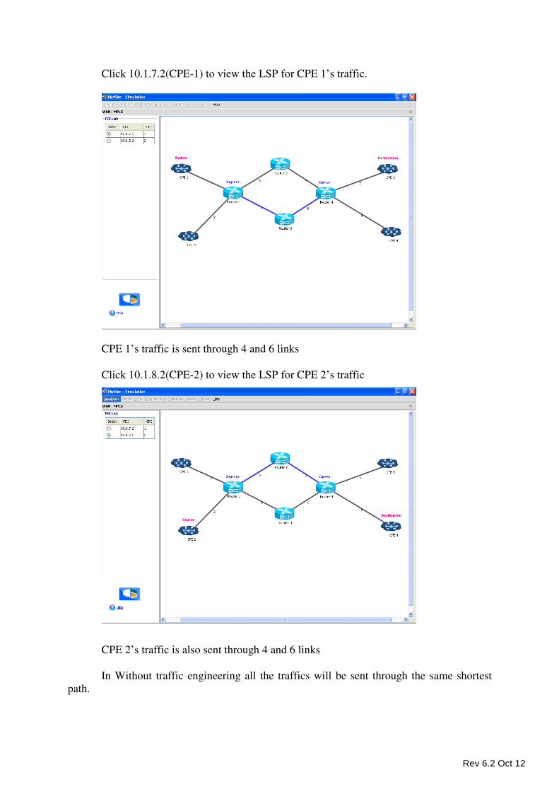
Click 10.1.7.2(CPE-1) to view the LSP for CPE 1’s traffic.
CPE 1’s traffic is sent through 4 and 6 links
Click 10.1.8.2(CPE-2) to view the LSP for CPE 2’s traffic
CPE 2’s traffic is also sent through 4 and 6 links
In Without traffic engineering all the traffics will be sent through the same shortest
path.
Rev 6.2 Oct 12

Inference:
In Traffic Engineered MPLS network, according to the traffic constraint different
traffics will be sent through different paths
But in without traffic engineering, all traffics will be sent through same shortest path.
Transmission Control Protocol (TCP)
New Experiments
In the Simulation menu select � New � WAN � TCP.
To perform experiments in TCP, the following steps should be followed,
• Create Scenario
• Set CPE Properties
• Set Link Properties
• Set Router Properties
• Remove Devices (or) Links
• Simulate
Create Scenario
Adding CPE (Customer Premise Equipment) - Click on the TCP CPE icon, drag and
drop the TCP CPE on the environment builder.
Adding Router - Click on the TCP Router icon, drag and drop the Router on the
environment builder. A Router here has eight Ports in which eight devices can be connected.
Establishing Connections between TCP CPE and Router - To establish a connection
follow these steps,
• The connection between the two TCP CPEs cannot be made in the network.
• On clicking the two devices connection can be made.
• The connection possibilities are as follows,
o CPE to Router and
o Router to Router.
Rev 6.2 Oct 12
Set CPE (Customer Premises Equipment) Properties
Right Click on the appropriate node to select Properties. Then, click on Application 1 to
modify properties.
Transmission Type: This indicates the type of transmission made by this session. Only
Point to Point Transmission is supported.
Destination: This property indicates the Destination CPE.
Traffic Type: This property indicates the type of traffic.
Data
Packet Size
Distribution: Only Constant distribution is available in this version.
Packet Size: Sets the size of the packets being generated by the Constant distribution.
Inter Arrival Time: This indicates the time gap between packets.
Traffic Pattern: Only Backlog is available in this version since the packets are
transmitted only on receipt of acknowledgements.
Click OK to accept the user entered values. Click on the close button at the top right
corner to exit the screen.
Transport Layer
Congestion Control: By default Old Tahoe is available. This can be modified to Tahoe.
Window size (Bytes): Either 11680 or 23360 can be selected as the Window size.
Network Layer
IP Address: Set the IP Address of the Nodes by selecting the appropriate values.
Subnet Mask: Enter a suitable subnet mask in this field.
Modifying/Viewing/Accepting Properties
On opening an already configured properties of an application the input fields will be
frozen (i.e. the input cannot be changed).To modify these values click on the Modify
button in the screen. Now the input value can be changed. Click on the Accept button, the
modified values will be saved.
Rev 6.2 Oct 12
This View button is enabled once the Accept Button is clicked. To view the given values,
click on the View button.
Set Link Properties
CPE to Router Link - To set the property values right click the Link between CPE to
Router and select Properties option. There are 4 property options that are available. They
are,
Error Rate (BER) - This property defines the rate at which the data is affected by error
in the network. The values that can be selected are 10^-6, 10^-7, 10^-8, 10^-9 and No
Error. By default the Error Rate is 10^-6.10^-6 means one error in every 1000000 bits
transmitted.
Physical Medium - This property defines the type of Physical Medium that is used in
the network. The types of Physical Medium used in this simulation are E0, T1, E1, T2
and E2. By default E0 is entered.
Data Rate (Mbps) - This property defines the rate at which the link transmits data. Based
on the type of Physical Medium the value of Data Rate is automatically calculated and
substituted. By default 0.064 Mbps is entered. Changes cannot be made to this property.
Distance (Kms) - This property defines the Distance between two devices in
Kilometers. By default 1Km is entered. A 4 digit value is the maximum Distance that
can be entered.
Router to Router Link - To change the property values right click the Link between
Router to Router and click Properties. There are 4 options for which changes can be made.
They are,
Error Rate (BER) - This property defines the rate at which the data is affected by error
in the network. The values that can be selected are 10^-6, 10^-7, 10^-8, 10^-9 and No
Error. By default the Error Rate is 10^-6.10^-6 means one error in every 1000000 bits
transmitted.
Physical Medium - This property defines the type of Physical Medium used in the
network. The Physical Medium that is used in connecting 2 Routers is a CAT5.
Data Rate (Mbps) - This property defines the rate at which the Link transmits data. The
two types of Data Rate that can be selected are, 10 and 100 Mbps. By default 10Mbps
is entered.
Rev 6.2 Oct 12
Distance (km) - This property defines the Distance between two devices in Kilometers.
By default 1Km is entered. A 4 digit value is the maximum Distance that can be entered.
Set Router Properties
Router Properties - To change any property, right click on the appropriate Router to get
the option window and click Properties.
Ports Properties - The number of ports available in a Router are 8. For each Port in a
Router the following properties are available,
IP Address - The IP Address obtained automatically. If Port 1 is selected then the IP
Address would be“10.1.1.1”. Changes can be made by entering values less than 255.
Subnet Mask - By default the value that is found in the Subnet Mask field is
“255.255.255.0”.
Connected To - This property gives the Router CPE that is connected to that Port (i.e.
If the CPE1 is connected to Port1, then when Port1 is selected CPE1 would be
displayed).
Router Properties
Buffer Size (KB) - This property defines the Buffer size that should be selected. Click
on the drop down button to avail the values. The values that are available are, “8, 16, 32,
64, 128, 256, 512, 1024, 2048 and 4096 (KB)”. 8KB is the default value.
Scheduling Type - Here the type of scheduler required can be selected. The Scheduling
Type available is FIFO. Changes cannot be made.
Routing Properties - The options available under Routing Properties are,
Routing Method - By default Static Routing method is used.
Data Link Layer - The options available under this property is,
Protocol Type - By default the Protocol Type found here is Ethernet. Here changes
cannot be made.
MAC Address - The Address of the particular router port.
Remove Devices (or) Links
Remove Link - Right click on the appropriate Link / Connection and click Remove.
Remove CPE - Right click on the appropriate Router CPE and click Remove.
Rev 6.2 Oct 12
Remove Router - Right click on the appropriate Router and click Remove.
Note -
• First remove the connecting Link.
• Next remove the Router / CPE. The removal of the Router / CPE can be done
after the connecting link has been removed.
Simulate - After creating the Scenario the following steps need to be followed,
• Click on Validate button.
• Click on Simulate button.
• Select the Simulation End Time and then click on “OK” button to start the
Simulation.
NetSim - TCP
Sample Experiments - User can understand the internal working of TCP through these
sample experiments. Each sample experiment covers:
• Procedure
• Sample Inputs
• Output
• Comparison chart
• Inference
Sample Experiment 1
Objective:
During client-server TCP downloads study the throughputs of Slow start + Congestion
avoidance (also known as Old Tahoe) and Fast Retransmit (also known as Tahoe),
Congestion Control Algorithms.
Index Objective
Experiment 1
During client-server TCP downloads study the throughputs of Slow
start + Congestion avoidance (also known as Old Tahoe) and Fast
Retransmit (also known as Tahoe), Congestion Control Algorithms.
Rev 6.2 Oct 12
Theory:
One of the important functions of a TCP Protocol is congestion control in the network. Given
below is a description of how Old Tahoe and Tahoe variants (of TCP) control congestion.
Old Tahoe:
Congestion can occur when data arrives on a big pipe (i.e. a fast LAN) and gets sent out
through a smaller pipe (i.e. a slower WAN). Congestion can also occur when multiple input
streams arrive at a router whose output capacity is less than the sum of the inputs. Congestion
avoidance is a way to deal with lost packets.
The assumption of the algorithm is that the packet loss caused by damaged is very small
(much less than 1%), therefore the loss of a packet signals congestion somewhere in the
network between the source and destination. There are two indications of packets loss: a
timeout occurring and the receipt of duplicate ACKs
Congestion avoidance and slow start are independent algorithms with different objectives.
But when congestion occurs TCP must slow down its transmission rate and then invoke slow
start to get things going again. In practice they are implemented together.
Congestion avoidance and slow start requires two variables to be maintained for each
connection: a Congestion Window (i.e. cwnd) and a Slow Start Threshold Size (i.e. ssthresh).
Old Tahoe algorithm is the combination of slow start and congestion avoidance. The
combined algorithm operates as follows,
1. Initialization for a given connection sets cwnd to one segment and ssthresh to 65535
bytes.
2. When congestion occurs (indicated by a timeout or the reception of duplicate ACKs),
one-half of the current window size (the minimum of cwnd and the reciever’s advertised
window, but at least two segments) is saved in ssthresh. Additionally, if the congestion is
indicated by a timeout, cwnd is set to one segment (i.e. slow start).
3. When new data is acknowledged by the other end, increase cwnd, but the way it increases
depends on whether TCP is performing slow start or congestion avoidance.
If cwnd is less than or equal to ssthresh, TCP is in slow start. Else TCP is performing
congestion avoidance. Slow start continues until TCP is halfway to where it was when
congestion occurred (since it recorded half of the window size that caused the problem in step
2). Then congestion avoidance takes over.
Slow start has cwnd begins at one segment and be incremented by one segment every time an
ACK is received. As mentioned earlier, this opens the window exponentially: send one
Rev 6.2 Oct 12
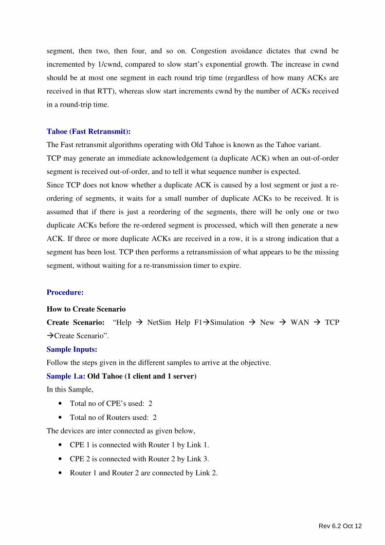
segment, then two, then four, and so on. Congestion avoidance dictates that cwnd be
incremented by 1/cwnd, compared to slow start’s exponential growth. The increase in cwnd
should be at most one segment in each round trip time (regardless of how many ACKs are
received in that RTT), whereas slow start increments cwnd by the number of ACKs received
in a round-trip time.
Tahoe (Fast Retransmit):
The Fast retransmit algorithms operating with Old Tahoe is known as the Tahoe variant.
TCP may generate an immediate acknowledgement (a duplicate ACK) when an out-of-order
segment is received out-of-order, and to tell it what sequence number is expected.
Since TCP does not know whether a duplicate ACK is caused by a lost segment or just a re-
ordering of segments, it waits for a small number of duplicate ACKs to be received. It is
assumed that if there is just a reordering of the segments, there will be only one or two
duplicate ACKs before the re-ordered segment is processed, which will then generate a new
ACK. If three or more duplicate ACKs are received in a row, it is a strong indication that a
segment has been lost. TCP then performs a retransmission of what appears to be the missing
segment, without waiting for a re-transmission timer to expire.
Procedure:
How to Create Scenario
Create Scenario: “Help � NetSim Help F1�Simulation � New � WAN � TCP
�Create Scenario”.
Sample Inputs:
Follow the steps given in the different samples to arrive at the objective.
Sample 1.a: Old Tahoe (1 client and 1 server)
In this Sample,
• Total no of CPE’s used: 2
• Total no of Routers used: 2
The devices are inter connected as given below,
• CPE 1 is connected with Router 1 by Link 1.
• CPE 2 is connected with Router 2 by Link 3.
• Router 1 and Router 2 are connected by Link 2.
Rev 6.2 Oct 12
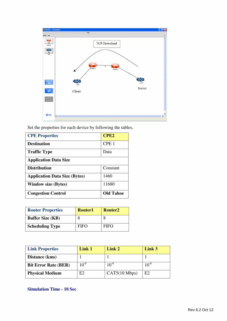
Set the properties for each device by following the tables,
CPE Properties CPE2
Destination CPE 1
Traffic Type Data
Application Data Size
Distribution Constant
Application Data Size (Bytes) 1460
Window size (Bytes) 11680
Congestion Control Old Tahoe
Link Properties Link 1 Link 2 Link 3
Distance (kms) 1 1 1
Bit Error Rate (BER) 10-6
10-6
10-6
Physical Medium E2 CAT5(10 Mbps) E2
Simulation Time - 10 Sec
Router Properties Router1 Router2
Buffer Size (KB) 8 8
Scheduling Type FIFO FIFO
Rev 6.2 Oct 12
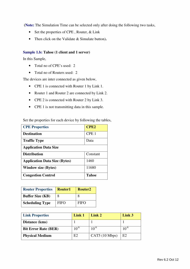
(Note: The Simulation Time can be selected only after doing the following two tasks,
• Set the properties of CPE , Router, & Link
• Then click on the Validate & Simulate button).
Sample 1.b: Tahoe (1 client and 1 server)
In this Sample,
• Total no of CPE’s used: 2
• Total no of Routers used: 2
The devices are inter connected as given below,
• CPE 1 is connected with Router 1 by Link 1.
• Router 1 and Router 2 are connected by Link 2.
• CPE 2 is connected with Router 2 by Link 3.
• CPE 1 is not transmitting data in this sample.
Set the properties for each device by following the tables,
CPE Properties CPE2
Destination CPE 1
Traffic Type Data
Application Data Size
Distribution Constant
Application Data Size (Bytes) 1460
Window size (Bytes) 11680
Congestion Control Tahoe
Link Properties Link 1 Link 2 Link 3
Distance (kms) 1 1 1
Bit Error Rate (BER) 10-6
10-6
10-6
Physical Medium E2 CAT5 (10 Mbps) E2
Router Properties Router1 Router2
Buffer Size (KB) 8 8
Scheduling Type FIFO FIFO
Rev 6.2 Oct 12
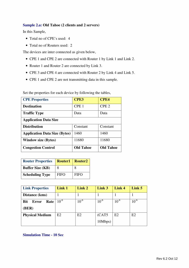
Sample 2.a: Old Tahoe (2 clients and 2 servers)
In this Sample,
• Total no of CPE’s used: 4
• Total no of Routers used: 2
The devices are inter connected as given below,
• CPE 1 and CPE 2 are connected with Router 1 by Link 1 and Link 2.
• Router 1 and Router 2 are connected by Link 3.
• CPE 3 and CPE 4 are connected with Router 2 by Link 4 and Link 5.
• CPE 1 and CPE 2 are not transmitting data in this sample.
Set the properties for each device by following the tables,
CPE Properties CPE3 CPE4
Destination CPE 1 CPE 2
Traffic Type Data Data
Application Data Size
Distribution Constant Constant
Application Data Size (Bytes) 1460 1460
Window size (Bytes) 11680 11680
Congestion Control Old Tahoe Old Tahoe
Router Properties Router1 Router2
Buffer Size (KB) 8 8
Scheduling Type FIFO FIFO
Link Properties Link 1 Link 2 Link 3 Link 4 Link 5
Distance (kms) 1 1 1 1 1
Bit Error Rate
(BER)
10-6
10-6
10-6
10-6
10-6
Physical Medium E2 E2 (CAT5
10Mbps)
E2 E2
Simulation Time - 10 Sec
Rev 6.2 Oct 12
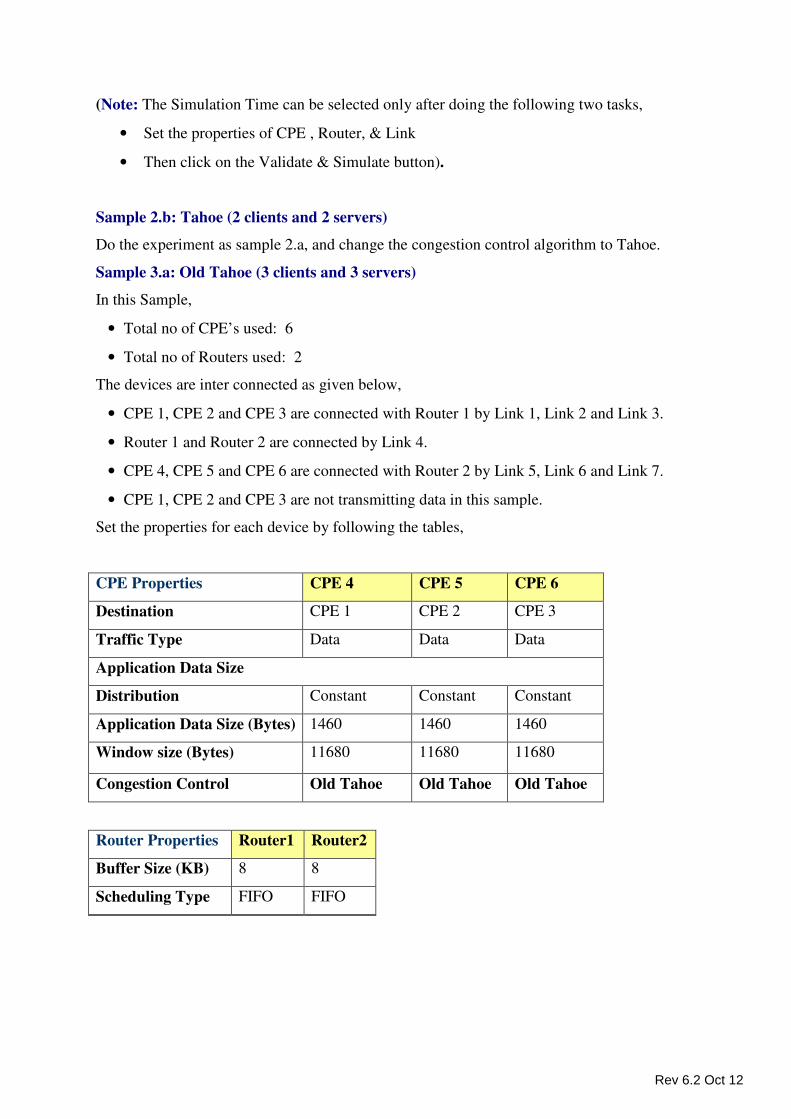
(Note: The Simulation Time can be selected only after doing the following two tasks,
• Set the properties of CPE , Router, & Link
• Then click on the Validate & Simulate button).
Sample 2.b: Tahoe (2 clients and 2 servers)
Do the experiment as sample 2.a, and change the congestion control algorithm to Tahoe.
Sample 3.a: Old Tahoe (3 clients and 3 servers)
In this Sample,
• Total no of CPE’s used: 6
• Total no of Routers used: 2
The devices are inter connected as given below,
• CPE 1, CPE 2 and CPE 3 are connected with Router 1 by Link 1, Link 2 and Link 3.
• Router 1 and Router 2 are connected by Link 4.
• CPE 4, CPE 5 and CPE 6 are connected with Router 2 by Link 5, Link 6 and Link 7.
• CPE 1, CPE 2 and CPE 3 are not transmitting data in this sample.
Set the properties for each device by following the tables,
CPE Properties CPE 4 CPE 5 CPE 6
Destination CPE 1 CPE 2 CPE 3
Traffic Type Data Data Data
Application Data Size
Distribution Constant Constant Constant
Application Data Size (Bytes) 1460 1460 1460
Window size (Bytes) 11680 11680 11680
Congestion Control Old Tahoe Old Tahoe Old Tahoe
Router Properties Router1 Router2
Buffer Size (KB) 8 8
Scheduling Type FIFO FIFO
Rev 6.2 Oct 12
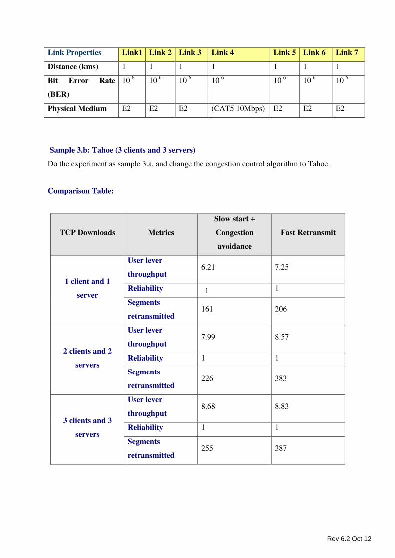
Link Properties Link1 Link 2 Link 3 Link 4 Link 5 Link 6 Link 7
Distance (kms) 1 1 1 1 1 1 1
Bit Error Rate
(BER)
10-6
10-6
10-6
10-6
10-6
10-6
10-6
Physical Medium E2 E2 E2 (CAT5 10Mbps) E2 E2 E2
Sample 3.b: Tahoe (3 clients and 3 servers)
Do the experiment as sample 3.a, and change the congestion control algorithm to Tahoe.
Comparison Table:
TCP Downloads Metrics
Slow start +
Congestion
avoidance
Fast Retransmit
1 client and 1
server
User lever
throughput 6.21 7.25
Reliability 1
1
Segments
retransmitted 161 206
2 clients and 2
servers
User lever
throughput 7.99 8.57
Reliability 1 1
Segments
retransmitted 226 383
3 clients and 3
servers
User lever
throughput 8.68 8.83
Reliability 1 1
Segments
retransmitted 255 387
Rev 6.2 Oct 12
Inference:
User lever throughput: User lever throughput of Fast Retransmit is higher when compared
then the Old Tahoe (SS + CA). This is because, if a segment is lost due to error, Old Tahoe
waits until the RTO Timer expires to retransmit the lost segment, whereas Tahoe (FR)
retransmits the lost segment immediately after getting three continuous duplicate ACK’s.
This results in the increased segment transmission, and therefore throughput is higher in the
case of Tahoe.
Reliability: The main feature of transmission control protocol is reliability. The reliability
can be the ratio of number of segments that reach the destination to the number of segments
transmitted in source. TCP ensures the reliability in the form of retransmission of those
segments that are errored. Irrespective of SS + CA or FR algorithm, the reliability of the
system is 1.
Segments retransmitted
As explained ion the inference on user level throughput, the segments re-transmitted of a FR
algorithm are higher than the SS + CA algorithm
User Datagram Protocol (UDP)
New Experiments
In the Simulation menu select Simulation � New � WAN � UDP.
To perform experiments in UDP, the following steps should be followed,
• Create Scenario
• Set CPE Properties
• Set Link Properties
• Set Router Properties
• Remove Devices (or) Links
• Simulate
Create Scenario
Adding CPE (Customer Premise Equipment) - Click on the Router CPE icon, drag
and drop the Router CPE on the environment builder.
Rev 6.2 Oct 12
Adding Router - Click on the Router icon, drag and drop the Router on the
environment builder. By default a Router has eight ports.
Establishing Connections between Router CPE and Router - The steps for to be
followed are as follows,
• The connections between the two Router CPEs cannot be made in the
network.
• On clicking the two devices connection can be made.
• The connection possibilities are,
o CPE to Router and
o Router to Router.
Set CPE (Customer Premises Equipment) Properties
Right Click on the appropriate node to select Properties. Inside the properties’ window
click on Application 1 to modify its properties.
Transmission Type
This indicates the type of transmission made by this session, only Point to Point
Transmission can be made.
Destination
This property indicates the Destination CPE.
Traffic Type
This property indicates the type of traffic. The traffic can either be Voice or Data.
Voice
Codec
Codec is the component of any voice system that translates between analog speech
and the bits used to transmit them. Every codec transmits a burst of data in a packet
that can be reconstructed into voice. Three different standards of voice codec’s are
given which can be selected depending on the variations required.
Service Type
• CBR - CBR stands for Constant Bit Rate. Packets of constant size are generated at
constant inter arrival times.
• VBR - VBR stands for Variable Bit Rate. The two types of Suppression Model that
can be selected are,
• Deterministic
Rev 6.2 Oct 12
• Markov Chain
• Success Ratio (%)
Click OK to accept the user entered values. Click on the close button at the top right
corner to exit the screen.
Data
Packet Size
Distribution: The options available for distribution are,
• Constant
• Exponential
Mean Packet Size (Bytes): Sets the size of the packets being generated by the
Constant distribution. The range of values that can be entered are between 10 to
10000 bytes. By default 1472 bytes is entered.
Inter Arrival Time
This indicates the time gap between packets.
Distribution : The options available for distribution are,
• Constant
• Exponential
• Uniform
Mean Inter Arrival Time: Enter the average inter-arrival time between packets. A
lower inter-arrival time would lead to a higher generation rate and the vice versa. The
range of values that can be entered are between 1000 to 20000 Micro Sec. By default
20000 Micro Sec is entered.
Click OK to accept the user entered values. Click on the close button at the top right
corner to exit the screen.
Network Layer
IP Address: Set the IP Address of the Nodes by selecting the appropriate values.
Subnet Mask: Give the valid values in this field.
Modifying/Viewing/Accepting Properties
On opening an already configured properties of an application the input fields will be
frozen (i.e. the input cannot be changed).To modify these values click on the Modify
button in the screen. Now the input value can be changed. Click on the Accept button, the
modified values will be saved.
This View button is enabled once the Accept Button is clicked. To view the given values,
click on the View button.
Rev 6.2 Oct 12
Set Link Properties
CPE to Router Link - To set the property values right click the Link between CPE to
Router and select Properties option. There are 4 property options that are available.
They are,
Error Rate (BER) - This property defines the rate at which the data is affected by
error in the network. The values that can be selected are 10^-6, 10^-7, 10^-8, 10^-9
and No Error. By default the Error Rate is 10^-6.10^-6 means one error in every
1000000 bits transmitted.
Physical Medium - This property defines the type of Physical Medium that is used
in the network. The types of Physical Medium used in this simulation are E0, T1,
E1, T2 and E2. By default E0 is entered.
Data Rate (Mbps) - This property defines the rate at which the link transmits data.
Based on the type of Physical Medium the value of Data Rate is automatically
calculated and substituted. By default 0.064 Mbps is entered. Changes cannot be
made to this property.
Distance (Kms) - This property defines the Distance between two devices in
Kilometers. By default 1Km is entered. A 4 digit value is the maximum Distance
that can be entered.
Router to Router Link –
To change the property values right click the Link between Router to Router and click
Properties. There are 4 options for which changes can be made. They are,
Error Rate (BER) - This property defines the rate at which the data is affected by
error in the network. The values that can be selected are 10^-6, 10^-7, 10^-8, 10^-9
and No Error. By default the Error Rate is 10^-6.10^-6 means one error in every
1000000 bits transmitted.
Physical Medium - This property defines the type of Physical Medium used in the
network. The Physical Medium that is used in connecting 2 Routers is a CAT5.
Data Rate (Mbps) - This property defines the rate at which the Link transmits data.
The two types of Data Rate that can be selected are, 10 and 100 Mbps. By default
10Mbps is entered.
Rev 6.2 Oct 12
Distance (km) - This property defines the Distance between two devices in
Kilometers. By default 1Km is entered. A 4 digit value is the maximum Distance
that can be entered.
Set Router Properties
Router Properties - To change any property, right click on the appropriate Router to
get the option window and click Properties.
Ports Properties - The number of ports available in a Router are 8. For each Port in a
Router the following properties are available,
Ip Address - The Ip Address must be filled up with a valid Ip Address. By default
the Ip Address that would be filled is “10.1.5.1”.
Subnet Mask - By default the value that is found in the Subnet Mask field is
“255.255.255.0”.
Connected To - This property gives the Router CPE that is connected to that Port
(i.e. If the CPE1 is connected to Port1, then when Port1 is selected CPE1 would be
displayed).
Router Properties
Buffer Size (KB) - This property defines the Buffer size that should be selected.
Click on the drop down button to avail the values. The values that are available are,
“8, 16, 32, 64, 128, 256, 512, 1024, 2048 and 4096 (KB)”. 8KB is the default value.
Scheduling Type - Here the type of scheduler required can be selected. The 2 types
of Scheduling Type are Priority and FIFO. By default Priority is available.
Data Link Layer - The options available under this property is,
Protocol Type - By default the Protocol Type found here is Ethernet. Here changes
cannot be made.
Remove Devices (or) Links
Remove Link - Right click on the appropriate Link and click Remove.
Remove Router CPE - Right click on the appropriate Router CPE and click Remove.
Remove Router - Right click on the appropriate Router and click Remove.
Rev 6.2 Oct 12
Note -
• First remove the connecting Link.
• Next remove the Router / CPE. The removal of the Router / CPE can be done
after the connecting link has been removed.
Simulate - After creating the Scenario the following steps need to be followed,
• Click on Validate button.
• Click on Simulate button.
• Select the Simulation End Time and then click on “OK” button to start the
Simulation.
X.25
New Experiments
In the Simulation menu select Simulation � New � WAN � X.25
To perform experiments in X.25, the following steps should be followed,
• Create Scenario
• Set CPE Properties
• Set Link Properties
• Set Switch Properties
• Remove Devices (or) Links
• Simulate
Create Scenario
Adding CPE (Customer Premise Equipment) - Click on the X.25 CPE icon, drag and
drop the X.25 CPE on the environment builder.
Adding Switch - Click on the Switch icon, drag and drop the Switch on the
environment builder. By default a Switch has eight ports.
Establishing Connections between X.25 CPE and Switch - The steps for to be followed
are as follows,
• The connections between the two X.25 CPEs cannot be made in the network.
• On clicking the two devices connection can be made.
• The connection possibilities are,
Rev 6.2 Oct 12
o CPE to Switch and
o Switch to Switch.
Set CPE (Customer Premises Equipment) Properties
Right Click on the appropriate node to select Properties. Inside the properties’ window click
on Application 1 to modify its properties.
Transmission Type
This indicates the type of transmission made by this session, only Point to Point
Transmission can be made.
Destination
This property indicates the Destination CPE.
Traffic Type
This property indicates the type of traffic. The traffic can either be Voice or Data.
Voice
Codec
Codec is the component of any voice system that translates between analog speech
and the bits used to transmit them. Every codec transmits a burst of data in a packet
that can be reconstructed into voice. Five different standards of voice codec’s are
given which can be selected depending on the variations required.
Service Type
• CBR - CBR stands for Constant Bit Rate. Packets of constant size are generated at
constant inter arrival times.
• VBR - VBR stands for Variable Bit Rate. The two types of Suppression Model
that can be selected are,
• Deterministic
• Markov Chain
Click OK to accept the user entered values. Click on the close button at the top
right corner to exit the screen.
Data
Packet Size
Distribution: The options available for distribution are,
• Constant
• Exponential
Mean Packet Size (Bytes): Sets the size of the packets being generated by the chosen
distribution. The range of values that can be entered are between 65 to 1500 bytes. By
default 1500 bytes is entered.
Rev 6.2 Oct 12
Inter Arrival Time
This indicates the time gap between packets.
Distribution: The options available for distribution are,
• Constant
• Exponential
• Uniform
Mean Inter Arrival Time: Enter the average inter-arrival time between packets. A
lower inter-arrival time would lead to a higher generation rate and the vice versa. The
range of values that can be entered are between 1000 to 20000 Micro Sec. By default
20000 Micro Sec is entered.
Click OK to accept the user entered values. Click on the close button at the top right
corner to exit the screen.
Data Link Layer
Virtual Circuit: This option consists of
• Switched (by default this option is set)
• Permanent
ARQ: This options consists of
• Stop and Wait
• Go Back N
• Selective Repeat
Modifying/Viewing/Accepting Properties
On opening an already configured properties of an application the input fields will be
frozen (i.e. the input cannot be changed).To modify these values click on the Modify
button in the screen. Now the input value can be changed. Click on the Accept button, the
modified values will be saved.
This View button is enabled once the Accept Button is clicked. To view the given values,
click on the View button.
Set Link Properties
Error Rate (BER) - This property defines the rate at which the data is affected by error
in the network. The values that can be selected are 10^-6, 10^-7, 10^-8, 10^-9 and No
Error. By default the Error Rate is 10^-6.10^-6 means one error in every 1000000 bits
transmitted.
Rev 6.2 Oct 12
Physical Medium - This property defines the type of Physical Medium that is used in
the network. The types of Physical Medium used in this simulation are E0, T1, E1, T2
and E2. By default E0 is entered.
Data Rate (Mbps) - This property defines the rate at which the link transmits data. Based
on the type of Physical Medium the value of Data Rate is automatically calculated and
substituted. By default 0.064 Mbps is entered. Changes cannot be made to this property.
Distance (Kms) - This property defines the Distance between two devices in
Kilometers. The range of values which can be entered are between 1 to 9999 Kms. By
default 1Km is entered. A 4 digit value is the maximum Distance that can be entered.
Set Switch Properties
Right click on the appropriate Switch and click Properties.
Port Properties - The Port Properties that are mentioned below are common to all the
Ports available in a Switch.
ARQ - Automatic Repeat reQuest consists of the following options,
• Stop and Wait
• Go Back N
• Selective Repeat
Buffer Size (KB) - This property specifies size of the buffer for that port on Switch.
Options available are � “8, 16, 32, 64, 128, 256, 512, 1024, 2048 and 4096”. Default
value is 8KB.
Remove Devices (or) Links
Remove Link - Right click on the appropriate Link and click Remove.
Remove X.25 CPE - Right click on the appropriate X.25 CPE and click Remove.
Remove X.25 Switch - Right click on the appropriate X.25 Switch and click Remove.
Note -
• First remove the connecting Link.
• Next remove the Switch / CPE. The removal of the Switch / CPE can be done after
the connecting link has been removed.
Simulate - After creating the Scenario the following steps need to be followed,
• Click on Validate button.
• Click on Simulate button.
Rev 6.2 Oct 12
• Select the Simulation End Time and then click on “OK” button to start the
Simulation.
Wi MAX – IEEE 802.16 - 2004
New Experiments
In the Simulation menu select � New � WMAN � Fixed Wi-MAX
To perform experiments in Wi-MAX, the following steps should be followed,
• Create Scenario
• Set Subscriber Properties
• Set Base Station (BS) Properties
• Remove Devices
• Simulate
Create Scenario
Adding Base Station - Click on the Base Station icon and drag it onto the environment
builder.
Adding Subscriber -
• Click on the Subscriber icon and drag and drop it on the Base Station coverage
area.
• Subscriber cannot be placed on another Subscriber. It has to be dragged and placed
on the Base Station coverage area.
Set Base Station (BS) Properties
Right click on the appropriate Base Station (BS) and click Properties. Options available
are,
Wireless Properties - Under Wireless Properties tab the options available are,
Connected To - This property defines the Wireless medium connected to the Base
Station (BS). A default value is already entered; hence no changes can be done.
Communication - This property defines the Communication mode of the network. By
default, a WiMAX network works in Half Duplex. This property cannot be changed.
Wi-MAX Standard – IEEE 802.16-2004
This standard is followed for modeling Data link Layer and Physical Layer.
Data Link Layer - Under Data Link Layer the sub-options available are,
Rev 6.2 Oct 12
MAC Address - A default value has been coded in, hence no change can be made.
Scheduling Technique – FIFO is set as scheduling technique.
Physical Layer - Under Physical Layer the sub-options available are,
Transmission type - This property specifies that the OFDM is used as a
Transmission technology.
Total Number of Sub Carrier (NFFT) – This property defines the total number of
sub carrier in the Channel. By default Total Number of Sub Carrier found is 256
Number of Used Sub Carries (Nused) – This property defines the Number of used
sub carrier in the channel. By default Total Number of used sub carrier found is 192
Modulation Technique – This property defines the Modulation Technique used in
transmission. By default BPSK is set as Modulation Technique. QPSK, 16QAM and
64 QAM are other modulation Technique can be selectable by user.
Coding Rate – This property defines the coding rate used in transmission. By default
1/2 is set as coding rate for BPSK Modulation Technique. 1/2 and 3/4 is used as other
coding rate for QPSK, 16 QAM and 64 QAM Modulation Technique.
Downlink to Uplink Ratio – This property denotes Downlink and Uplink
Transmission Ratio. 1:1 is set as default Downlink to Uplink Ratio.
Frequency (GHz) - This property defines the frequency allotted for the channel. By
default Frequency (GHz) found is 3.5 GHz.
Nominal Channel Bandwidth (MHz) – This property denotes Channel Bandwidth
used for Transmission. 3.5 MHz is set as default Nominal Channel Bandwidth. 5.5
and 10 MHz are the other channel bandwidth can be selectable by user.
Sampling Factor (n) – This property is used to find the symbol time. 8/7 is set as
default Sampling Factor.
Guard Interval (G) – This property is used to ensure the transmission interference.
1/4 is set as default Guard Interval.
OFDM Frame Duration – This property is used to denote the OFDM frame duration
value. 10 ms is set as default OFDM Frame duration value. User can also select 20 ms
as OFDM frame duration value.
Rev 6.2 Oct 12
Channel Error – This property denotes the Channel Error characteristics. By default
None is set as Channel Error.
Set Subscriber Properties
Right Click on the appropriate Subscriber to select Properties. Inside the properties window
click on Application1 to modify its properties.
Transmission Type
This indicates the type of transmission made by this session, Point to Point.
Destination
This property indicates the Destination Subscriber.
Traffic Type
This property indicates the type of traffic. The traffic can either be Voice.
Voice
Call Details
Call Interval Time (Secs)
This property denotes the Call Interval Time. Each Call begins exponentially with
mean call inter arrival time. 300 sec is set as default Call Inter Arrival Time. User can
select 450 secs or 600 secs as Call Interval Time.
Call Duration (Secs)
This property denotes how long the call continues. By default 60 secs is set as Call
duration. User can select 120 and 240 secs as their call duration value.
Codec
Codec is the component of any voice system that translates between analog speech
and the bits used to transmit them. Every codec transmits a burst of data in a packet
that can be reconstructed into voice.
Service Type
• CBR - CBR stands for Constant Bit Rate. Packets of constant size are
generated at constant inter arrival times.
Click OK to accept the user entered values. Click on the close button at the top right
corner to exit the screen.
Packet Size
Packet Size (Bytes): Based on Codec Selection Packet Size can be set.
Inter Arrival Time
This indicates the time gap between packets. Based on Codec selection Inter Arrival
Time can be set.
Rev 6.2 Oct 12
Generation Rate
This denotes the Traffic Generation rate by the Subscriber. Based on Packet size and
Inter Arrival Time Generation Rate can be set.
Click OK to accept the user entered values. Click on the close button at the top right
corner to exit the screen.
Transport Layer
Protocol
This property denotes which protocol is used in Transport layer. By Default UDP is
used as Transport Layer protocol.
Segment Size (Bytes)
This property denotes maximum amount of data that a single packet contains. By
default 1472 is set as default segment size.
Network Layer
Protocol
This property denotes the protocol used in Network layer. By default IPV4 is used as
Network Layer protocol.
IP Address
This property denotes the IP Address set for Subscriber. Based on Subscriber Id, IP
Address varies.
Subnet Mask
This property denotes the default subnet mask used in network. By Default
255.255.255.0 is set as Subnet Mask.
Rev 6.2 Oct 12
Wi-MAX Standard – IEEE 802.16 -2004
Data Link Layer
MTU (Bytes)
This property denotes Maximum Transmission Unit set for Data link Layer protocol.
1500 Bytes is set as Default MTU for Ethernet Protocol.
QoS Class
This property denotes which QoS Class service is used in Subscriber. By default UGS is
set as QoS Class which supports Voice Over IP and offers fixed size unsolicited data
grants on periodic basis.
MAC Address
This property denotes MAC Address value set for Subscriber. This MAC Address value
varies for each Subscriber.
Convergence Sub Layer
This property denotes the transport type for packet. Packet CS is set as Convergence Sub
Layer which is used for the transport of all packet-based protocols such as the Internet
Protocols (IP).
Physical Layer
Transmission Type
This property denotes the transmission type used in Subscriber. By Default OFDM is set
as Transmission Type for Subscriber.
Click Accept button.
Modifying/Viewing/Accepting Properties
On opening an already configured properties of an application the input fields will be
frozen (i.e. the input cannot be changed).To modify these values click on the Modify
button in the screen. Now the input value can be changed. Click on the Accept button, the
modified values will be saved.
This View button is enabled once the Accept Button is clicked. To view the given values,
click on the View button.
Rev 6.2 Oct 12
Remove Devices
Remove Subscriber - Right click on the appropriate Subscriber and click Remove.
Remove Base Station - Right click on the appropriate Base Station and click Remove.
Note:
• If a Subscriber which has already data traffic is removed, all traffic originating
from this Subscriber is also deleted.
• In cases where the Base Station is in a network, firstly all Subscriber need to be
removed. Subsequently the Base Station can be removed.
Simulate - After creating the Scenario the following steps need to be followed,
• Click on Validate button.
• Click on Simulate button.
• Select the Simulation End Time and then click on “OK” button to start the
Simulation.
NetSim – Wi-MAX
Sample Experiments - User can understand the internal working of Wi MAX through these
sample experiments. Each sample experiment covers:
• Procedure
• Sample Inputs
• Output
• Comparison chart
• Inference
Index Objective
Experiment 1
To study the Call Blocking probability of a Wi-MAX (IEEE 802.16 –
2004) network varies for UGS (Unsolicited Grant Service) QoS Class
as the number of transmitting SSs increase beyond the bandwidth limit.
Rev 6.2 Oct 12
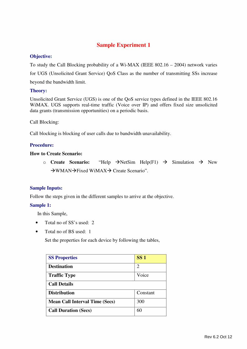
Sample Experiment 1
Objective:
To study the Call Blocking probability of a Wi-MAX (IEEE 802.16 – 2004) network varies
for UGS (Unsolicited Grant Service) QoS Class as the number of transmitting SSs increase
beyond the bandwidth limit.
Theory:
Unsolicited Grant Service (UGS) is one of the QoS service types defined in the IEEE 802.16
WiMAX. UGS supports real-time traffic (Voice over IP) and offers fixed size unsolicited
data grants (transmission opportunities) on a periodic basis.
Call Blocking:
Call blocking is blocking of user calls due to bandwidth unavailability.
Procedure:
How to Create Scenario:
o Create Scenario: “Help �NetSim Help(F1) � Simulation � New
�WMAN�Fixed WiMAX� Create Scenario”.
Sample Inputs:
Follow the steps given in the different samples to arrive at the objective.
Sample 1:
In this Sample,
• Total no of SS’s used: 2
• Total no of BS used: 1
Set the properties for each device by following the tables,
SS Properties SS 1
Destination 2
Traffic Type Voice
Call Details
Distribution Constant
Mean Call Interval Time (Secs) 300
Call Duration (Secs) 60
Rev 6.2 Oct 12
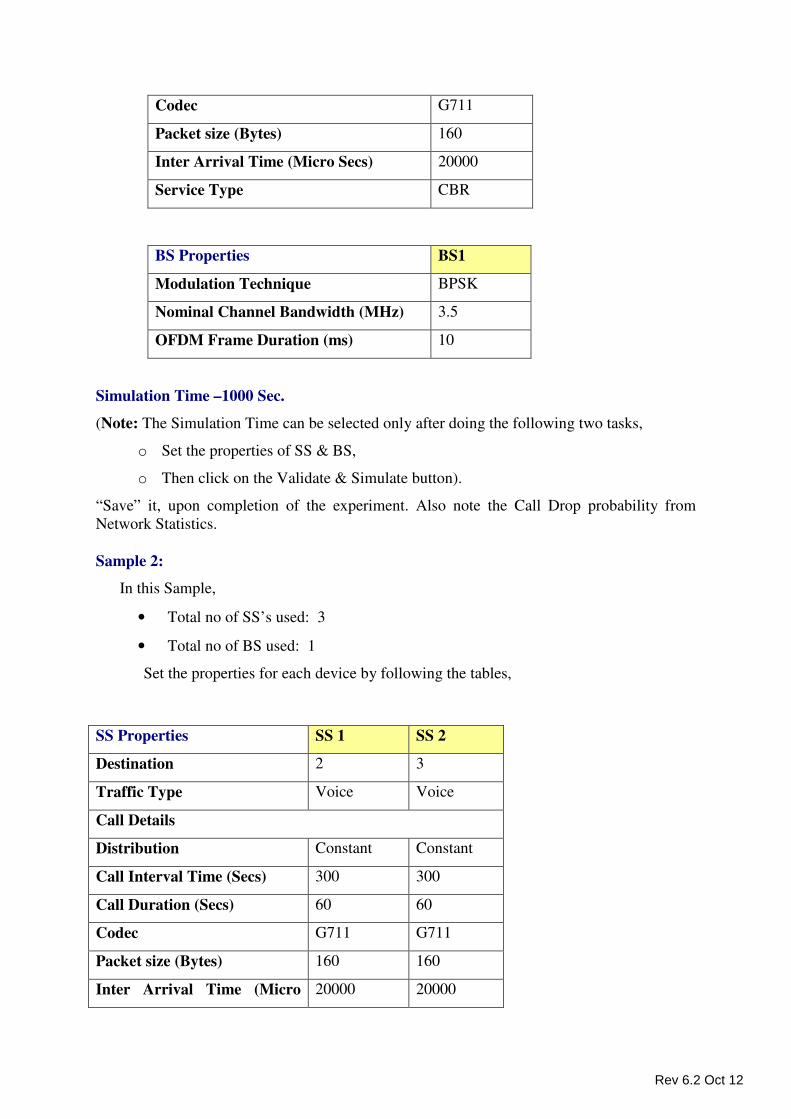
Codec G711
Packet size (Bytes) 160
Inter Arrival Time (Micro Secs) 20000
Service Type CBR
BS Properties BS1
Modulation Technique BPSK
Nominal Channel Bandwidth (MHz) 3.5
OFDM Frame Duration (ms) 10
Simulation Time –1000 Sec.
(Note: The Simulation Time can be selected only after doing the following two tasks,
o Set the properties of SS & BS,
o Then click on the Validate & Simulate button).
“Save” it, upon completion of the experiment. Also note the Call Drop probability from
Network Statistics.
Sample 2:
In this Sample,
• Total no of SS’s used: 3
• Total no of BS used: 1
Set the properties for each device by following the tables,
SS Properties SS 1 SS 2
Destination 2 3
Traffic Type Voice Voice
Call Details
Distribution Constant Constant
Call Interval Time (Secs) 300 300
Call Duration (Secs) 60 60
Codec G711 G711
Packet size (Bytes) 160 160
Inter Arrival Time (Micro 20000 20000
Rev 6.2 Oct 12
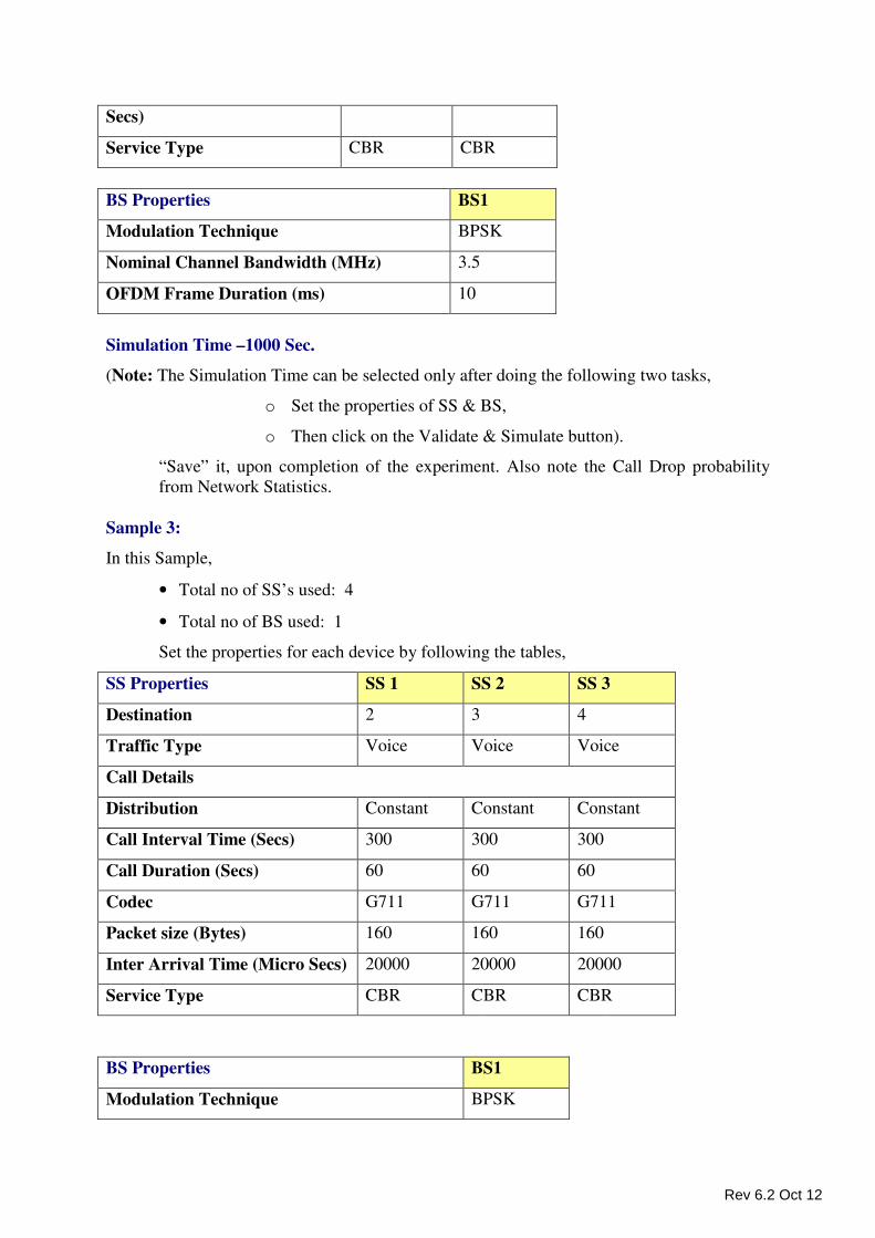
Secs)
Service Type CBR CBR
BS Properties BS1
Modulation Technique BPSK
Nominal Channel Bandwidth (MHz) 3.5
OFDM Frame Duration (ms) 10
Simulation Time –1000 Sec.
(Note: The Simulation Time can be selected only after doing the following two tasks,
o Set the properties of SS & BS,
o Then click on the Validate & Simulate button).
“Save” it, upon completion of the experiment. Also note the Call Drop probability
from Network Statistics.
Sample 3:
In this Sample,
• Total no of SS’s used: 4
• Total no of BS used: 1
Set the properties for each device by following the tables,
SS Properties SS 1 SS 2 SS 3
Destination 2 3 4
Traffic Type Voice Voice Voice
Call Details
Distribution Constant Constant Constant
Call Interval Time (Secs) 300 300 300
Call Duration (Secs) 60 60 60
Codec G711 G711 G711
Packet size (Bytes) 160 160 160
Inter Arrival Time (Micro Secs) 20000 20000 20000
Service Type CBR CBR CBR
BS Properties BS1
Modulation Technique BPSK
Rev 6.2 Oct 12
Nominal Channel Bandwidth (MHz) 3.5
OFDM Frame Duration (ms) 10
Simulation Time –1000 Sec.
(Note: The Simulation Time can be selected only after doing the following two tasks,
o Set the properties of SS & BS,
o Then click on the Validate & Simulate button).
“Save” it, upon completion of the experiment. Also note the Call Drop
probability from Network Statistics.
Sample 4:
In this Sample,
• Total no of SS’s used: 5
• Total no of BS used: 1
Set the properties for each device by following the tables,
SS Properties SS 1 SS 2 SS 3 SS 4
Destination 2 3 4 5
Traffic Type Voice Voice Voice Voice
Call Details
Distribution Constant Constant Constant Constant
Call Interval Time (Secs) 300 300 300 300
Call Duration (Secs) 60 60 60 60
Codec G711 G711 G711 G711
Packet size (Bytes) 160 160 160 160
Inter Arrival Time (Micro Secs) 20000 20000 20000 2000
Service Type CBR CBR CBR CBR
BS Properties BS1
Modulation Technique BPSK
Nominal Channel Bandwidth (MHz) 3.5
OFDM Frame Duration (ms) 10
Rev 6.2 Oct 12
Simulation Time –1000 Sec.
(Note: The Simulation Time can be selected only after doing the following two tasks,
o Set the properties of SS & BS,
o Then click on the Validate & Simulate button).
“Save” it, upon completion of the experiment. Also note the Call Drop probability
from Network Statistics.
Sample 5:
In this Sample,
• Total no of SS’s used: 6
• Total no of BS used: 1
Set the properties for each device by following the tables,
SS Properties SS 1 SS 2 SS 3 SS 4 SS 5
Destination 2 3 4 5 6
Traffic Type Voice Voice Voice Voice Voice
Call Details
Distribution Constant Constant Constant Constant Constant
Call Interval Time (Secs) 300 300 300 300 300
Call Duration (Secs) 60 60 60 60 60
Codec G711 G711 G711 G711 G711
Packet size (Bytes) 160 160 160 160 160
Inter Arrival Time (Micro
Secs)
20000 20000 20000 20000 20000
Service Type CBR CBR CBR CBR CBR
BS Properties BS1
Modulation Technique BPSK
Nominal Channel Bandwidth (MHz) 3.5
OFDM Frame Duration (ms) 10
Simulation Time –1000 Sec.
Rev 6.2 Oct 12
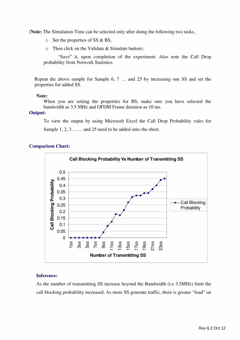
(Note: The Simulation Time can be selected only after doing the following two tasks,
o Set the properties of SS & BS,
o Then click on the Validate & Simulate button).
“Save” it, upon completion of the experiment. Also note the Call Drop
probability from Network Statistics.
Repeat the above sample for Sample 6, 7 … and 25 by increasing one SS and set the
properties for added SS.
Note: When you are setting the properties for BS, make sure you have selected the
bandwidth as 3.5 MHz and OFDM Frame duration as 10 ms.
Output:
To view the output by using Microsoft Excel the Call Drop Probability vales for
Sample 1, 2, 3 …… and 25 need to be added onto the sheet.
Comparison Chart:
Call Blocking Probability Vs Number of Transmitting SS
0
0.05
0.1
0.15
0.2
0.25
0.3
0.35
0.4
0.45
0.5
1ss
3ss
5ss
7ss
9ss
11ss
13ss
15ss
17ss
19ss
21ss
23ss
Number of Transmitting SS
Call B
lockin
g P
rob
ab
ilit
y
Call BlockingProbability
Inference:
As the number of transmitting SS increase beyond the Bandwidth (i.e 3.5MHz) limit the
call blocking probability increased. As more SS generate traffic, there is greater “load” on
Rev 6.2 Oct 12
the network beyond the Bandwidth limit (3.5 MHz), this leads to increase in Call
blocking probability.
Based on Physical layer inputs,
Only 62 OFDM symbols are used to handle the all the calls. To handle one call, it
requires 17 OFDM symbols. So it can handle simultaneously 3 Calls request. If more than
three calls arrive, then the extra arrived calls are blocked.
1. From the graph we have seen the variation in call blocking probability as the
numbers of SS are increased from 1 to 25. The Calls generated by all SS are not
effectively handled by BS, because of Bandwidth unavailability (i.e 3.5 MHz)
2. In the graph we are getting a call drop variation in 11SS to 25 SS, because each SS
starts the first call exponentially.
Wireless Sensor Network (WSN)
New Experiments
In the Simulation menu select Simulation � New � WSN
To perform experiments in WSN, the following steps should be followed,
• Create Scenario
• Set Sink Node Properties
• Set Agent Properties
• Set Sensor Properties
• Set Environment Properties
• Remove Devices
• Simulate
Create Scenario
Adding Sink Node- Click on the Sink Node icon and drag and drop it onto the
environment builder.
Adding Sensor - Click on the Sensor Node icon and drag and drop it onto the
environment builder.
Adding Agent- Click on the Agent icon and drag and drop it onto the environment
builder.
Rev 6.2 Oct 12
Set Sink Node Properties
Right Click on the Sink Node to select Properties.
Network Layer - The options available under this property is,
Routing Information – Reactive (On-Demand Routing) the process to find a path is
only executed when a path is required by a node.
Routing Protocol- Dynamic Source Routing (DSR) which is a routing protocol, used in
wireless sensor networks.
Data Link Layer - The options available under this property is,
Protocol – IEEE 802.15.4 is a standard which specifies the physical layer and media access
control for low-rate wireless personal area networks (LR-WPANs).
Beacon Mode – Beacon Mode defines synchronization and reliability of the transmission
mechanism, whereas beaconless networks adopt a simple lightweight protocol based on
CSMA-CA. There are two options available, Enable/Disable. Default is set as enable
Beacon Order – Beacon Order, describes the interval at which the coordinator shall
transmit its beacon frames. 15 denotes that beacon mode is disabled, if Beacon mode is
enabled then the Beacon Order value can range from 0 to 14. Default Beacon Order
value is 15.
Superframe Order – Superframe Order describes the length of the active portion of the
superframe, which includes the beacon frame. This property will be there, only in case of
beacon mode is enabled. The value of Superframe Order should be less than 15. Default
value is 15.
GTS Mode - GTS (Guaranteed Time Slot) allows a device to operate on the channel
within a portion of the superframe that is dedicated (on the PAN) exclusively to that
device. This property will be there, only if beacon mode is enabled. By default the GTS
Mode is enabled.
Superframe Duration – The Superframe Duration (SD) is divided into 16 equally sized
time slots, during which data transmission is allowed. The SD can be further divided into
a Contention Access Period (CAP)and an optional Contention Free Period (CFP)
Rev 6.2 Oct 12

composed of Guaranteed Time Slots. A default value has been coded in; hence no change
can be made. The fixed value is 15.36 ms.
Battery Life Extension – The Battery Life Extension (BLE) subfield is 1 bit in length
and shall be set to one if frames transmitted to the beaconing device during its
CAP(Contention Access Period) are required to start on or before macBattLifeExtPeriods
full backoff periods after the IFS (inter frame space or spacing) period following the
beacon. Otherwise, the BLE subfield shall be set to 0. The options available are
True/False. This property will be there, only in case of beacon mode is enabled. By
default the Battery Life Extension mode is true.
Maximum Backoff Exponent – The maximum value of the backoff exponent (BE) in
the CSMA-CA algorithm. The Maximum Backoff Exponent value ranges from 3 to 8.
Default value is 5.
Minimum Backoff Exponent – The minimum value of the backoff exponent (BE) in the
CSMA-CA algorithm. The Minimum Backoff Exponent value rangse from 0 to Max BE.
Default value is 5.
Max Frame retries – The maximum number of retries allowed after a transmission
failure. The Max Frame retries value ranges from 0 to 7. By default the Max Frame
retries value is 3.
MAX CSMA Backoff - The maximum number of backoffs the CSMA-CA algorithm
will attempt before declaring a channel access failure. The MAX CSMA Backoff value
ranges from 0 to 5. Default value is 4.
Unit Backoff Period - The number of symbols forming the basic time period used by the
CSMA-CA algorithm. A default value has been coded in; hence no change can be made.
The value is 20 Symbols.
Min CAP length - The minimum number of symbols forming the CAP (contention
access period).This ensures that MAC commands can still be transferred to devices when
GTSs (Guaranteed Time Slot) are being used. A default value has been coded in; hence
no change can be made. The value is 440 Symbols
Rev 6.2 Oct 12
GTS descriptor Persistent Time - A default value has been coded in; hence no change
can be made. The GTS descriptor Persistent Time is 4 s.
Physical Layer - The options available under this property is,
Protocol – IEEE 802.15.4 Phy - IEEE 802.15.4 is a standard which specifies the
physical layer and media access control for low-rate wireless personal area networks (LR-
WPANs).
Frequency Band - Frequency bands are groupings of radio frequencies that are used by
mobile networks to communicate with mobile phones. A default value has been coded in;
hence no change can be made. The value is 2.4 GHz.
Data Rate - Data rate or bit rate is the number of bits that are conveyed or processed per
unit of time. A default value has been coded in; hence no change can be made. The value
is 250 kbps.
Chip Rate - The chip rate of a code is the number of pulses per second (chips per second)
at which the code is transmitted (or received). The chip rate is larger than the symbol rate,
meaning that one symbol is represented by multiple chips. A default value has been
coded in; hence no change can be made. The value is 2000 McPs.
Symbol Rate - In digital communications, symbol rate (also known as baud or
modulation rate) is the number of symbol changes (waveform changes or signaling
events) made to the transmission medium per second using a digitally modulated signal or
a line code. A default value has been coded in; hence no change can be made. The value
is 62.5 KSymbolsPS.
Modulation Technique - Offset quadrature phase-shift keying (OQPSK) is a variant of
phase-shift keying modulation using 4 different values of the phase to transmit. It is
sometimes called staggered quadrature phase-shift keying (SQPSK).
Min LIFS period - The minimum number of symbols forming a LIFS (Long Inter Frame
Spacing) period. A default value has been coded in; hence no change can be made. The
value is 40 Symbols.
Min SIFS period - The minimum number of symbols forming a SIFS (Short Inter Frame
Spacing) period. A default value has been coded in; hence no change can be made. The
value is 20 Symbols.
Rev 6.2 Oct 12
Unit Backoff Time - The number of symbols forming the basic time period used by the
CSMA-CA algorithm. A default value has been coded in; hence no change can be made.
The value is 20 Symbols.
Turn Around Time - The TX-to-RX turnaround time is defined as the shortest time
possible at the air interface from the trailing edge of the last chip (of the last symbol) of a
transmitted PPDU to the leading edge of the first chip (of the first symbol) of the next
received PPDU. The RX-to-TX turnaround time is defined as the shortest time possible at
the air interface from the trailing edge of the last chip (of the last symbol) of a received
PPDU to the leading edge of the first chip (of the first symbol) of the next transmitted
PPDU. A default value has been coded in; hence no change can be made. The value is 12
Symbols.
Phy SHR Duration – The duration of the synchronization header (SHR) in symbols for
the current PHY. The Values available are 3, 7, 10, and 40. By default Phy SHR
Duration is 3.
Phy Symbol Per Octet - The number of symbols per octet for the current PHY. The
Values available are 0.4, 1.6, 2, 8. By default phy symbol per octet is 0.4.
CCA mode
The following are the available options under CCA mode,
• Carrier Sense Only (by default this options is selected).
CCA (Clear Channel Assessment) shall report a busy medium only upon the
detection of a signal compliant with this standard with the same modulation and
spreading characteristics of the PHY that is currently in use by the device. This
signal may be above or below the ED threshold.
• Energy Detection
CCA shall report a busy medium upon detecting any energy above the ED
threshold.
• Carrier Sense with Energy Detection
CCA shall report a busy medium using a logical combination of Detection of a
signal with the modulation and spreading characteristics of this standard and
Energy above the ED threshold, where the logical operator may be AND/OR.
Rev 6.2 Oct 12
Receiver Sensitivity –Threshold input signal power that yields a specified PER
(packet error rate) conditions PSDU (PHY service data unit) length = 20 octets PER
less than 1% Power measured at antenna terminals. Interference not present The
Receiver Sensitivity Value should be less than 0. Default value is -85 dbm.
ED threshold - The receiver ED threshold is intended for use by a network layer as
part of a channel selection algorithm. It is an estimate of the received signal power
within the bandwidth of the channel. No attempt is made to identify or decode signals
on the channel. If the receive signal power is greater than the ED threshold value then
the channel selection algorithm will return false. The ED threshold Value should be
less than 0. Default value is -95 dbm.
Power Model - The options available under this property is,
Power Source - Power is got from battery.
Initial Power - Power is got from main line, and therefore the initial power is
assumed to be infinite.
Set Agent Properties
Right Click on the Agent and click Properties. Options available are,
Agent Properties
Mobility Model
Mobility – The options available are,
• Random Way Point (default option) - Random Way Point (RWP) model is a
commonly used synthetic model for mobility in networks. It is an elementary
model which describes the movement pattern of independent nodes by simple
terms.
• Random Walk - Random walk model is that of a random walk on a regular
lattice, where at each step the walk jumps to another site according to a
predefined probability distribution.
Velocity (m/s) - This property defines movement speed of the nodes. Velocity value
should be less than 100. Default value is 20 m/s.
Rev 6.2 Oct 12
Pause Time (sec) – This property specifies that the “Pause Time”. Nodes will
remain the same position for this time period.
Data logging – Data logging is the process of collecting the data, analyzing it, saving
and outputting the results of the collection and analysis. It has two options
Enable/Disable. If it is enabled the following two properties will be visible
o Data File Name – It denotes that the name of the data file where the sink node
stores the data.
o Path – It denotes the path, where the file is to be saved.
Sensing Interval (ms) – Sensing interval is the time difference between two sensor
events. Sensing Interval should be less than 5000 ms. Default value is 1000 ms.
Set Sensor Properties
Right Click on the appropriate Sensor to select Properties.
Network Layer - The options available under this property is,
Routing Information – Reactive: (On-Demand Routing) the process to find a path is
only executed when a path is required by a node.
Routing Protocol- Dynamic Source Routing (DSR) which is a routing protocol, used in
wireless sensor networks.
Data Link Layer - The options available under this property is,
Protocol - IEEE 802.15.4 is a standard which specifies the physical layer and media
access control for low-rate wireless personal area networks (LR-WPANs).
Mac Address - A Media Access Control address (MAC address) is a unique
identifier assigned to network interfaces for communications on the physical network
segment.
Retry Limit - This indicates the number of attempts that can be made by a frame.
This value varies range from 0 to 7.
Ack request – Frame transmitted with the Acknowledgment Request subfield of its
frame control field set to one shall be acknowledged by the recipient. It can be
enabled or disabled. By default it is enabled.
Physical Layer - The options available under this property is,
Rev 6.2 Oct 12
Protocol – IEEE 802.15.4 Phy is a standard which specifies the physical layer and
media access control for low-rate wireless personal area networks (LR-WPANs).
Transmitter Power - This property defines the power level of the Wireless device. It
ranges from 1 to 100 milli watts. Default value is 20 milli watts.
Sensor Range - A sensor is a device which receives and responds to a signal within a
particular range. This value should be less than 100m. Default value is 100 m.
Transmitter Radius - The transmission range of the device. This changes based on
environmental conditions. This value should be less than 100m. Default value is 100
m.
Receiver Sensitivity – Threshold input signal power that yields a specified PER
(packet error rate) Conditions PSDU (PHY service data unit) length = 20 octets PER
less than 1% Power measured at antenna terminals. Interference not present. Receiver
Sensitivity value should be less than 0. Default value is -85 dbm.
ED threshold – The receiver ED threshold is intended for use by a network layer as
part of a channel selection algorithm. It is an estimate of the received signal power
within the bandwidth of the channel. No attempt is made to identify or decode signals
on the channel. If the receive signal power is greater than the ED threshold value then
the channel selection algorithm will return false. ED threshold value should be less
than 0. Default value is -95 dbm.
Power Model - The options available under this property is,
Power Source –The options available under the power source is Battery or Main
Line.
Power Source- Main Line
Power gets from main line, the main line is the general-purpose alternating current
(AC) electric power supply.
Power Source - Battery - Power is got from battery. The options available under the
Battery is,
Energy harvesting – Energy harvesting (also known as power harvesting or energy
scavenging) is the process by which energy is derived from external sources (e.g.,
Rev 6.2 Oct 12
solar power, thermal energy, wind energy, and kinetic energy), captured, and stored
for small, wireless autonomous devices, like those used in wearable electronics and
wireless sensor networks. It can be on or off mode. Default it is on mode.
Recharging Current – The current flow during recharge. This property will be there
only if the Energy harvesting is in on mode. Default value is 0.4 mA.
Initial Energy – Initial energy stored in the battery. The Initial Energy value should
be less than 1000kW. Default value is 1000 kW.
Voltage – Voltage is a measure of the energy carried by the charge. The Voltage
value should be less than 10.0v. Default value is 3.6 V.
Transmitting Current –The current required for Transmission. The Transmitting
Current value should be less than 20mA. Default value is 8.8 mA.
Receiving Current –The current required for receive the data. The Receiving Current
value should be less than 20mA. Default value is 9.6 mA.
Idle Mode Current –The current flow during idle mode. The Idle Mode Current
value should be less than 20mA. Default value is 3.3 mA.
Sleep Mode Current - The current flow during sleep mode. The Sleep Mode Current
value should be less than 20mA. Default value is 0.237 mA.
Remove Devices (or) Links
Remove Sink Node - Right click on the appropriate Sink Node and click Remove.
Remove Sensor - Right click on the appropriate Sensor and click Remove.
Remove Agent - Right click on the appropriate Agent and click Remove.
Simulate - After creating the Scenario the following steps need to be followed,
• Click on Validate button.
• Click on Simulate button.
• Select the Simulation End Time and then click on “OK” button to start the
Simulation.
Rev 6.2 Oct 12
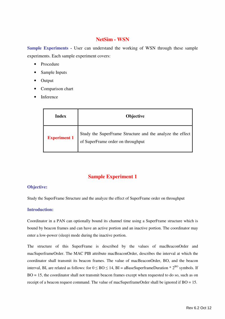
NetSim - WSN
Sample Experiments - User can understand the working of WSN through these sample
experiments. Each sample experiment covers:
• Procedure
• Sample Inputs
• Output
• Comparison chart
• Inference
Index Objective
Experiment 1 Study the SuperFrame Structure and the analyze the effect
of SuperFrame order on throughput
Sample Experiment 1
Objective:
Study the SuperFrame Structure and the analyze the effect of SuperFrame order on throughput
Introduction:
Coordinator in a PAN can optionally bound its channel time using a SuperFrame structure which is
bound by beacon frames and can have an active portion and an inactive portion. The coordinator may
enter a low-power (sleep) mode during the inactive portion.
The structure of this SuperFrame is described by the values of macBeaconOrder and
macSuperframeOrder. The MAC PIB attribute macBeaconOrder, describes the interval at which the
coordinator shall transmit its beacon frames. The value of macBeaconOrder, BO, and the beacon
interval, BI, are related as follows: for 0 ≤ BO ≤ 14, BI = aBaseSuperframeDuration * 2BO
symbols. If
BO = 15, the coordinator shall not transmit beacon frames except when requested to do so, such as on
receipt of a beacon request command. The value of macSuperframeOrder shall be ignored if BO = 15.
Rev 6.2 Oct 12
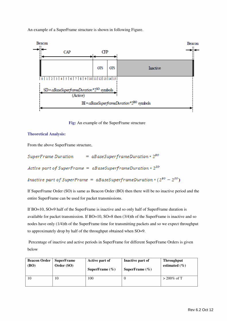
An example of a SuperFrame structure is shown in following Figure.
Fig: An example of the SuperFrame structure
Theoretical Analysis:
From the above SuperFrame structure,
If SuperFrame Order (SO) is same as Beacon Order (BO) then there will be no inactive period and the
entire SuperFrame can be used for packet transmissions.
If BO=10, SO=9 half of the SuperFrame is inactive and so only half of SuperFrame duration is
available for packet transmission. If BO=10, SO=8 then (3/4)th of the SuperFrame is inactive and so
nodes have only (1/4)th of the SuperFrame time for transmitting packets and so we expect throughput
to approximately drop by half of the throughput obtained when SO=9.
Percentage of inactive and active periods in SuperFrame for different SuperFrame Orders is given
below
Beacon Order
(BO)
SuperFrame
Order (SO)
Active part of
SuperFrame (%)
Inactive part of
SuperFrame (%)
Throughput
estimated (%)
10 10 100 0 > 200% of T
Rev 6.2 Oct 12
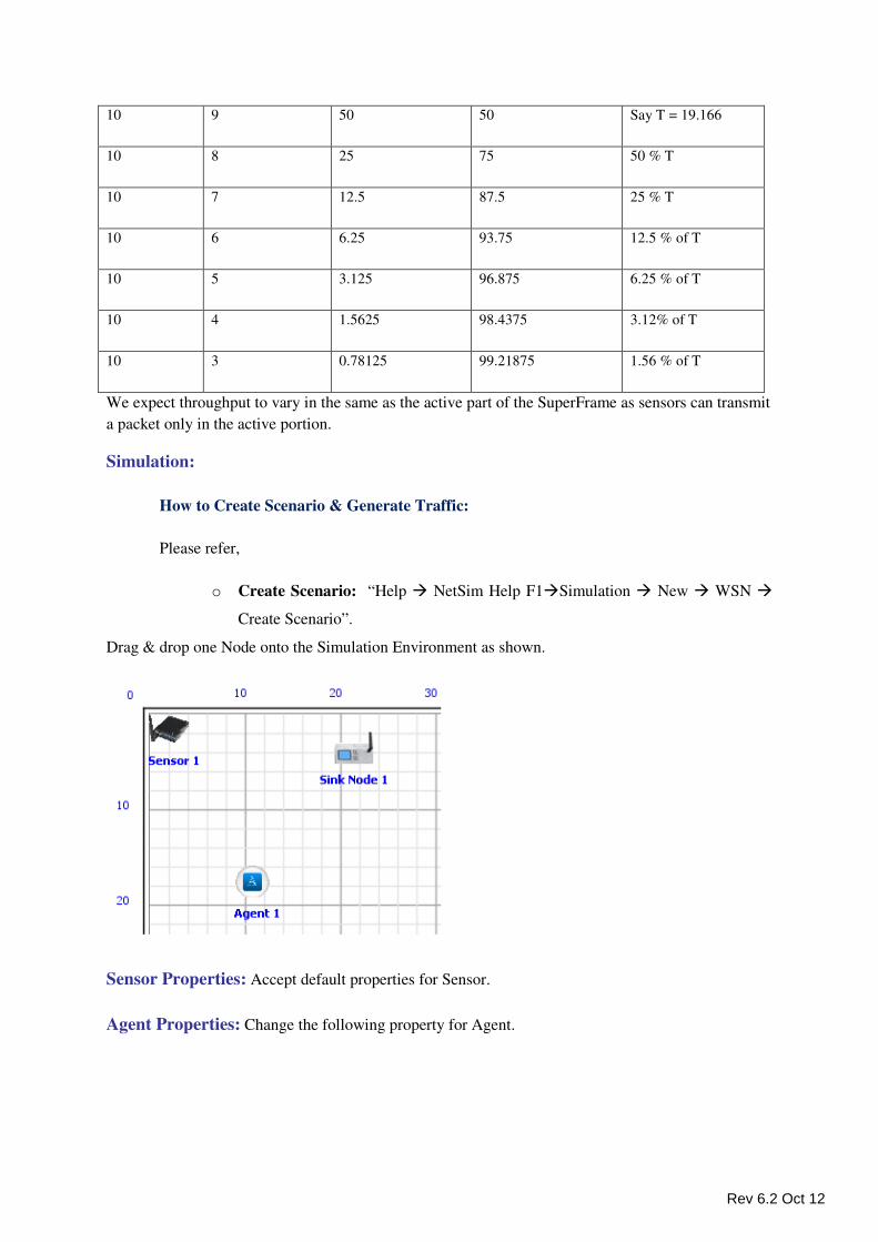
10 9 50 50 Say T = 19.166
10 8 25 75 50 % T
10 7 12.5 87.5 25 % T
10 6 6.25 93.75 12.5 % of T
10 5 3.125 96.875 6.25 % of T
10 4 1.5625 98.4375 3.12% of T
10 3 0.78125 99.21875 1.56 % of T
We expect throughput to vary in the same as the active part of the SuperFrame as sensors can transmit
a packet only in the active portion.
Simulation:
How to Create Scenario & Generate Traffic:
Please refer,
o Create Scenario: “Help � NetSim Help F1�Simulation � New � WSN �
Create Scenario”.
Drag & drop one Node onto the Simulation Environment as shown.
Sensor Properties: Accept default properties for Sensor.
Agent Properties: Change the following property for Agent.
Rev 6.2 Oct 12
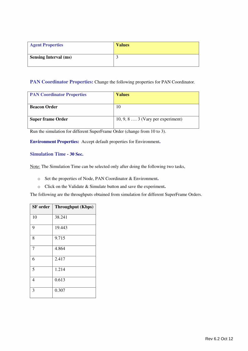
Agent Properties Values
Sensing Interval (ms) 3
PAN Coordinator Properties: Change the following properties for PAN Coordinator.
PAN Coordinator Properties Values
Beacon Order 10
Super frame Order 10, 9, 8 …. 3 (Vary per experiment)
Run the simulation for different SuperFrame Order (change from 10 to 3).
Environment Properties: Accept default properties for Environment.
Simulation Time - 30 Sec.
Note: The Simulation Time can be selected only after doing the following two tasks,
o Set the properties of Node, PAN Coordinator & Environment.
o Click on the Validate & Simulate button and save the experiment.
The following are the throughputs obtained from simulation for different SuperFrame Orders.
SF order Throughput (Kbps)
10 38.241
9 19.443
8 9.715
7 4.864
6 2.417
5 1.214
4 0.613
3 0.307
Rev 6.2 Oct 12
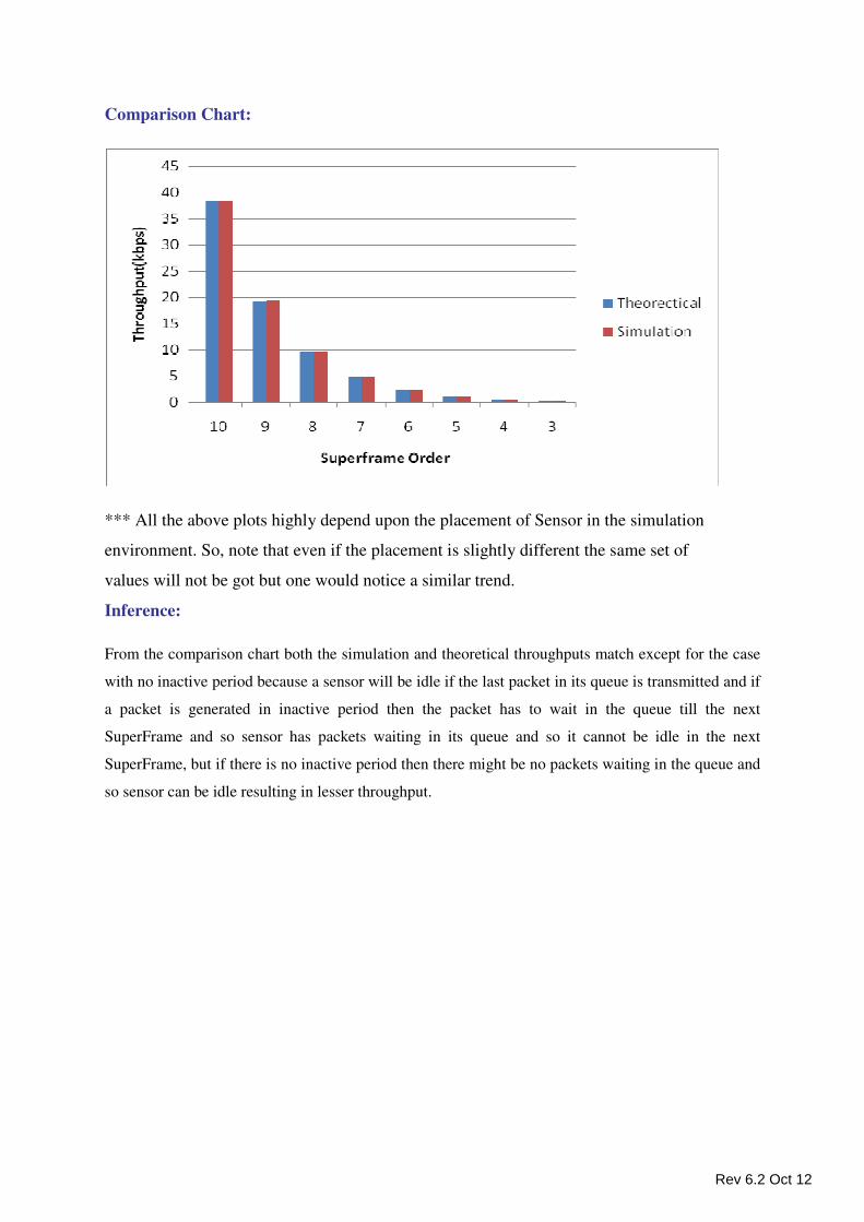
Comparison Chart:
*** All the above plots highly depend upon the placement of Sensor in the simulation
environment. So, note that even if the placement is slightly different the same set of
values will not be got but one would notice a similar trend.
Inference:
From the comparison chart both the simulation and theoretical throughputs match except for the case
with no inactive period because a sensor will be idle if the last packet in its queue is transmitted and if
a packet is generated in inactive period then the packet has to wait in the queue till the next
SuperFrame and so sensor has packets waiting in its queue and so it cannot be idle in the next
SuperFrame, but if there is no inactive period then there might be no packets waiting in the queue and
so sensor can be idle resulting in lesser throughput.
Rev 6.2 Oct 12
OPEN
Network
Select Network from Simulation ����Open menu to open saved experiments. The
following steps need to be followed,
• Select the User (Note: This option is available in Admin login only.)
• Select the Network. There are six options Cellular, LAN, PAN, WAN, WMAN and WSN. Choose based on the saved Experiment that needs to be opened.
• Select the Protocol.
• Select the Experiment that needs to be opened.
• Click on Ok button to open the selected Experiment. User can modify the existing Scenario, Simulate and Save it. Else Click on Cancel button to Exit the screen.
Metrics
Select Metrics from Simulation ����Open menu to open metrics results of the saved
experiments. The following steps need to be followed,
• Select the User (Note: This option is available in Admin login only. This option can be used to open experiments created by different users)
• Select the Network. There are six options LAN, PAN, WAN, WMAN, Cellular and WSN. Choose based on the saved Experiment that needs to be opened.
• Select the Protocol.
• Select the Experiment that needs to be opened.
• Click on Ok button to open the selected Experiment. User can modify the existing Scenario, Simulate and Save it. Else Click on Cancel button to Exit the screen.
Delete
In the Simulation menu select Delete/Delete All option to delete the saved Simulated
Experiments. To delete Experiments the user needs to follow the below given steps,
• Click the Delete/Delete All button to enter into the next window. When
Delete button is clicked only a single experiment can be deleted, whereas
Delete All button deletes all the saved experiments.
Rev 6.2 Oct 12
• In the next window,
o Select the Experiment Name that needs to be deleted.
o Click on Delete button to delete the selected Experiment, else click
on Cancel button to cancel deletion.
o After clicking on the Delete button a message appears which says
“Are you sure you want to delete this Experiment”. Click on Yes to
continue deleting the selected Experiment, else click on No to cancel
deleting.
o Click on OK button in the “The experiment is deleted” window.
Note:
• Admin User: An option called User Name is available only in when the User
has logged into Admin. This option can be made use for deleting experiments
which the Admin desires.
• Local User: A User who has a normal privilege other than Admin can delete
experiments only which are created by themselves.
Analytics
Under the Simulation menu click Analytics to view the Analytics screen. This module
is designed to enable inter and intra protocol comparison for different performance
metrics. A graphing engineer facilitates plotting of different performance metrics across
the different experiments. This can be used to infer/trend how changes in input
parameters affect network performance. An explanation of the use of the different fields
in the Analytics screen is detailed below,
• User: This Option can be made use of to compare different experiments created
by a single user. As Admin is a Super User, he/she can compare all the
experiments created by all the users. Things that cannot be done are,
o User to User comparison cannot be made, i.e. two or more different
experiments created by two or more different users cannot be compared.
o Experiments of LAN Protocols cannot be compared with experiments of WAN
Protocols.
Rev 6.2 Oct 12
• The six tabs on the top of the tool bar are -
o LAN - Click this tab when comparing the performances of LAN Protocols
o PAN - Click this tab when comparing the performances of PAN Protocols
o WAN - Click this tab when comparing the performances of WAN Protocols
o WMAN - Click this tab when comparing the performances of WMAN
Protocol
o Cellular - Click this tab when comparing the performances of Cellular
Protocol
o WSN - Click this tab when comparing the performances of WSN Protocol
• The Tool Bar functionalities are
o Select the Experiment - Experiments can be selected based on the tab (i.e.
LAN or PAN or WAN or WMAN or Cellular or WSN) selected. When one of
the tabs is selected, all the experiments saved under LAN Protocols are
listed. Click on the Experiment Name to add it onto the Metrics Table. Export
to .csv - Click on Export to .csv to export the Metrics Table to a “.csv”
format. This action button will export the contents to a “.csv” format that is
available.
o Print - Click on the Print option to print the Metrics Table. This action button
will get the Print dialogue box.
• The Graph Field
o Select the Metrics - Select the coordinates for Y-axis by clicking on the
dropdown menu.
o Graph - Based on the X-axis (i.e. Experiment selected) and Y-axis (i.e.
Metrics selected by using the dropdown menu above the graph), a Bar
graph would be plotted.
• The Metrics Table - This is the table that is generated when the Experiments
are selected using the Select the Experiment option. The following columns are
available in the Metrics Table,
o The first column in the Metrics Table consists of the Check Boxes that are
used to select (i.e. by default all the Experiments are selected) or deselect
the selected Experiments. If an Experiment is selected, then that Experiment
Rev 6.2 Oct 12
would be compared along with other Experiments, else the Experiment would
not be compared with other Experiments.
o The second column in the Metrics Table “X” button is available. This “X”
button is used for deleting the Experiment.
o Columns that follow are Experiment Name, Utilization (%), Effective
Utilization (%), Overhead (%), Loss(%), Unutilized(%), Delay(ms),
Queuing Delay(ms), Medium Access Time(ms) and Transmission
Time(ms).
o For cellular protocol, the columns are Experiment Name, Call generated,
Call processed, Call blocked, Call blocking probability, Number of
channel, Max channel Use, Average channel use, Handover attempt,
Successful handover, Unsuccessful handover, Call dropping
probability.
Rev 6.2 Oct 12
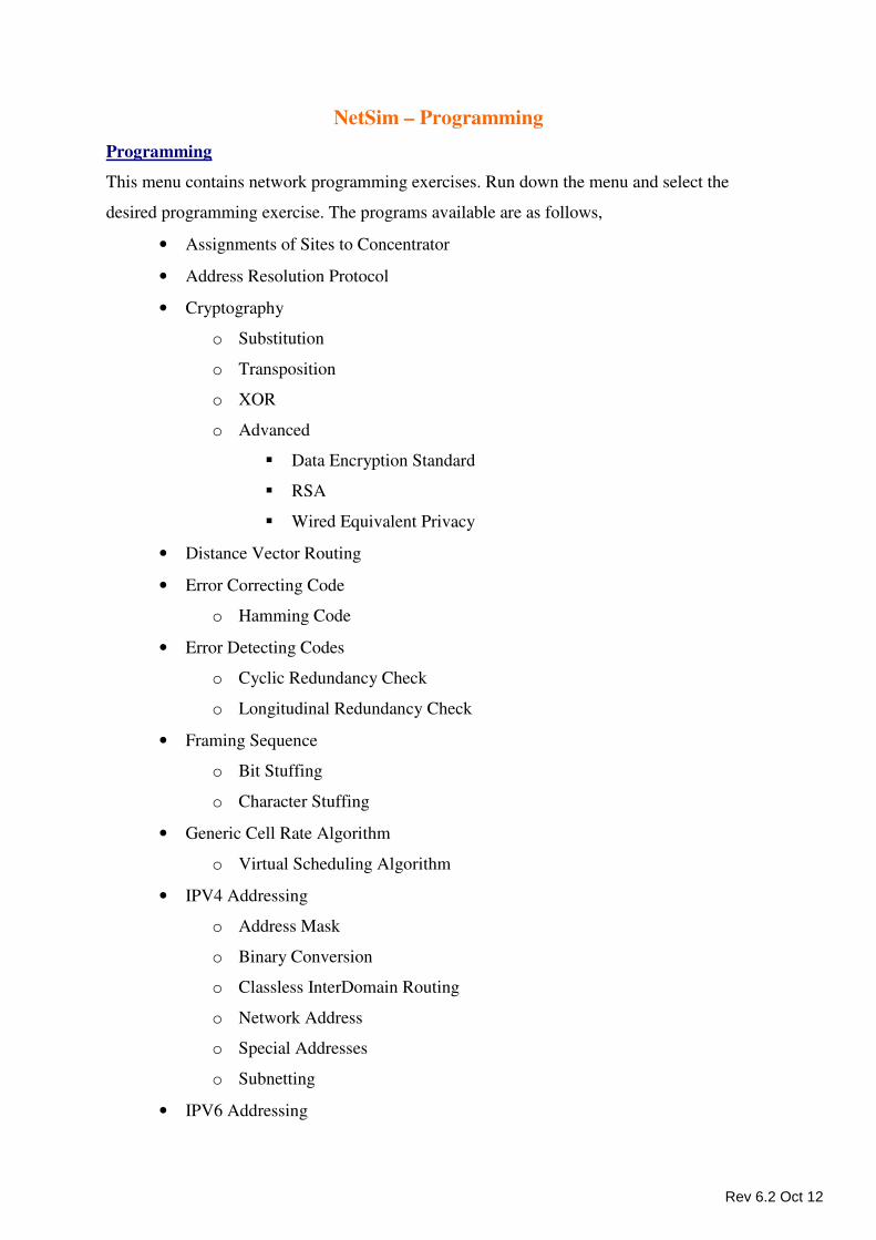
NetSim – Programming
Programming
This menu contains network programming exercises. Run down the menu and select the
desired programming exercise. The programs available are as follows,
• Assignments of Sites to Concentrator
• Address Resolution Protocol
• Cryptography
o Substitution
o Transposition
o XOR
o Advanced
� Data Encryption Standard
� RSA
� Wired Equivalent Privacy
• Distance Vector Routing
• Error Correcting Code
o Hamming Code
• Error Detecting Codes
o Cyclic Redundancy Check
o Longitudinal Redundancy Check
• Framing Sequence
o Bit Stuffing
o Character Stuffing
• Generic Cell Rate Algorithm
o Virtual Scheduling Algorithm
• IPV4 Addressing
o Address Mask
o Binary Conversion
o Classless InterDomain Routing
o Network Address
o Special Addresses
o Subnetting
• IPV6 Addressing
Rev 6.2 Oct 12
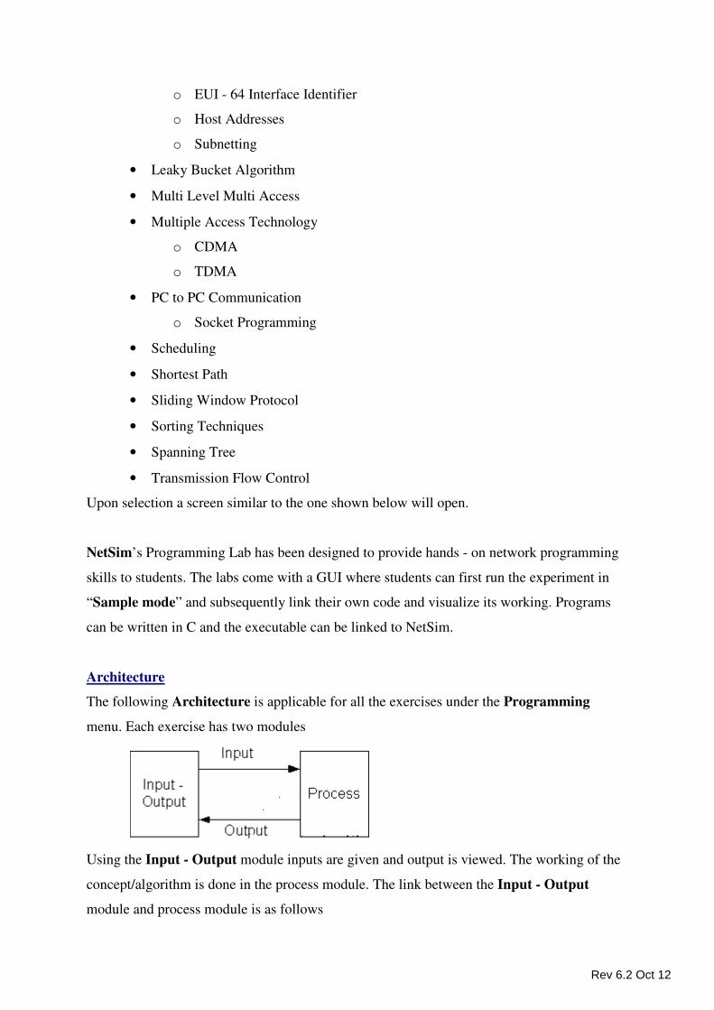
o EUI - 64 Interface Identifier
o Host Addresses
o Subnetting
• Leaky Bucket Algorithm
• Multi Level Multi Access
• Multiple Access Technology
o CDMA
o TDMA
• PC to PC Communication
o Socket Programming
• Scheduling
• Shortest Path
• Sliding Window Protocol
• Sorting Techniques
• Spanning Tree
• Transmission Flow Control
Upon selection a screen similar to the one shown below will open.
NetSim’s Programming Lab has been designed to provide hands - on network programming
skills to students. The labs come with a GUI where students can first run the experiment in
“Sample mode” and subsequently link their own code and visualize its working. Programs
can be written in C and the executable can be linked to NetSim.
Architecture
The following Architecture is applicable for all the exercises under the Programming
menu. Each exercise has two modules
Using the Input - Output module inputs are given and output is viewed. The working of the
concept/algorithm is done in the process module. The link between the Input - Output
module and process module is as follows
Rev 6.2 Oct 12
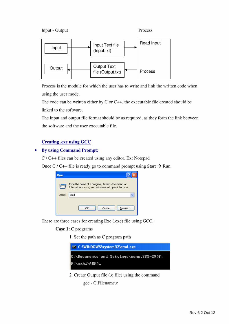
Input - Output Process
Process is the module for which the user has to write and link the written code when
using the user mode.
The code can be written either by C or C++, the executable file created should be
linked to the software.
The input and output file format should be as required, as they form the link between
the software and the user executable file.
Creating .exe using GCC
• By using Command Prompt:
C / C++ files can be created using any editor. Ex: Notepad
Once C / C++ file is ready go to command prompt using Start � Run.
There are three cases for creating Exe (.exe) file using GCC.
Case 1: C programs
1. Set the path as C program path
2. Create Output file (.o file) using the command
gcc - C Filename.c
Input
Output
Input Text file
(Input.txt)
Output Text
file (Output.txt)
Read Input
Process
Rev 6.2 Oct 12
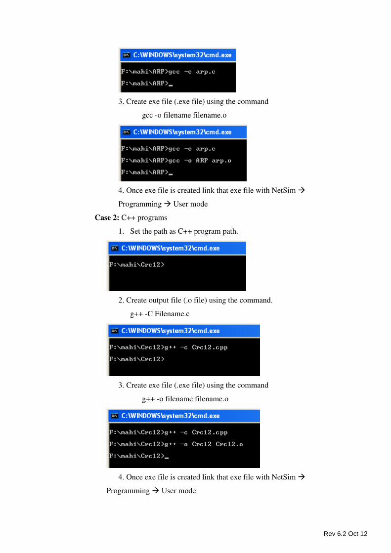
3. Create exe file (.exe file) using the command
gcc -o filename filename.o
4. Once exe file is created link that exe file with NetSim �
Programming � User mode
Case 2: C++ programs
1. Set the path as C++ program path.
2. Create output file (.o file) using the command.
g++ -C Filename.c
3. Create exe file (.exe file) using the command
g++ -o filename filename.o
4. Once exe file is created link that exe file with NetSim �
Programming � User mode
Rev 6.2 Oct 12
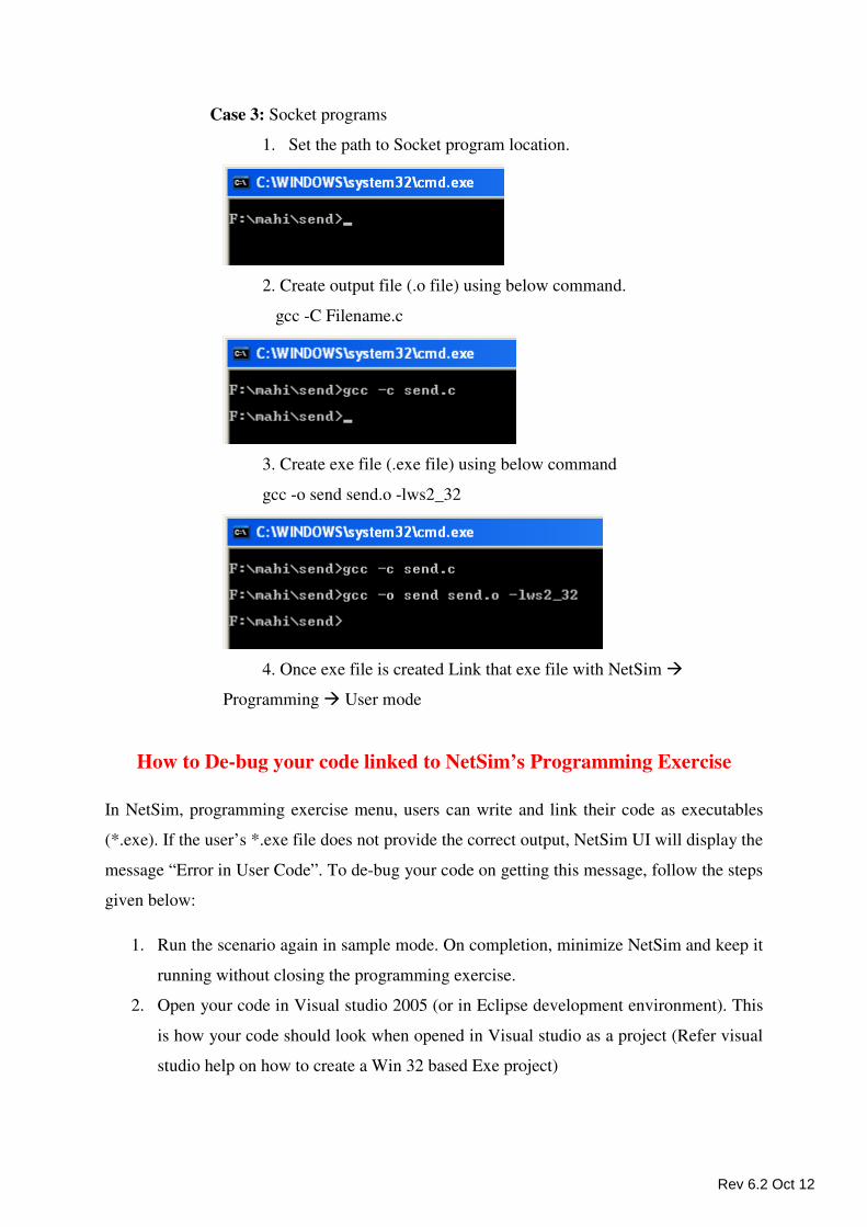
Case 3: Socket programs
1. Set the path to Socket program location.
2. Create output file (.o file) using below command.
gcc -C Filename.c
3. Create exe file (.exe file) using below command
gcc -o send send.o -lws2_32
4. Once exe file is created Link that exe file with NetSim �
Programming � User mode
How to De-bug your code linked to NetSim’s Programming Exercise
In NetSim, programming exercise menu, users can write and link their code as executables
(*.exe). If the user’s *.exe file does not provide the correct output, NetSim UI will display the
message “Error in User Code”. To de-bug your code on getting this message, follow the steps
given below:
1. Run the scenario again in sample mode. On completion, minimize NetSim and keep it
running without closing the programming exercise.
2. Open your code in Visual studio 2005 (or in Eclipse development environment). This
is how your code should look when opened in Visual studio as a project (Refer visual
studio help on how to create a Win 32 based Exe project)
Rev 6.2 Oct 12
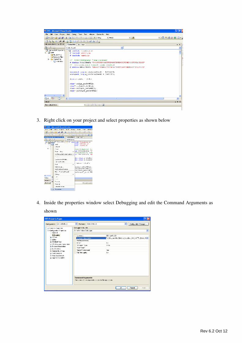
3. Right click on your project and select properties as shown below
4. Inside the properties window select Debugging and edit the Command Arguments as
shown
Rev 6.2 Oct 12
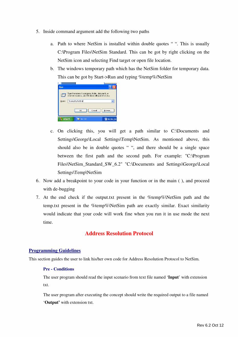
5. Inside command argument add the following two paths
a. Path to where NetSim is installed within double quotes “ “. This is usually
C:\Program Files\NetSim Standard. This can be got by right clicking on the
NetSim icon and selecting Find target or open file location.
b. The windows temporary path which has the NetSim folder for temporary data.
This can be got by Start->Run and typing %temp%/NetSim
c. On clicking this, you will get a path similar to C:\Documents and
Settings\George\Local Settings\Temp\NetSim. As mentioned above, this
should also be in double quotes “ “, and there should be a single space
between the first path and the second path. For example: "C:\Program
Files\NetSim_Standard_SW_6.2" "C:\Documents and Settings\George\Local
Settings\Temp\NetSim
6. Now add a breakpoint to your code in your function or in the main ( ), and proceed
with de-bugging
7. At the end check if the output.txt present in the %temp%\NetSim path and the
temp.txt present in the %temp%\NetSim path are exactly similar. Exact similarity
would indicate that your code will work fine when you run it in use mode the next
time.
Address Resolution Protocol
Programming Guidelines
This section guides the user to link his/her own code for Address Resolution Protocol to NetSim.
Pre - Conditions
The user program should read the input scenario from text file named ‘Input’ with extension
txt.
The user program after executing the concept should write the required output to a file named
‘Output’ with extension txt.
Rev 6.2 Oct 12
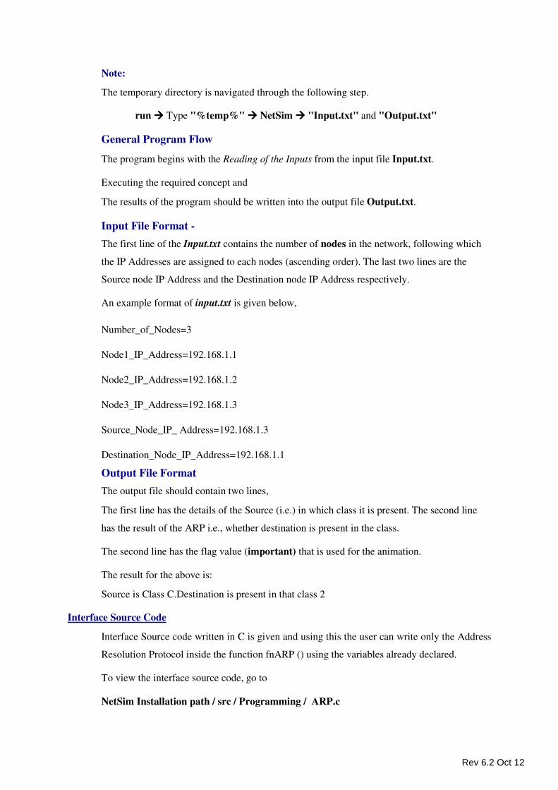
Note:
The temporary directory is navigated through the following step.
run ���� Type "%temp%" ���� NetSim ���� "Input.txt" and "Output.txt"
General Program Flow
The program begins with the Reading of the Inputs from the input file Input.txt.
Executing the required concept and
The results of the program should be written into the output file Output.txt.
Input File Format -
The first line of the Input.txt contains the number of nodes in the network, following which
the IP Addresses are assigned to each nodes (ascending order). The last two lines are the
Source node IP Address and the Destination node IP Address respectively.
An example format of input.txt is given below,
Number_of_Nodes=3
Node1_IP_Address=192.168.1.1
Node2_IP_Address=192.168.1.2
Node3_IP_Address=192.168.1.3
Source_Node_IP_ Address=192.168.1.3
Destination_Node_IP_Address=192.168.1.1
Output File Format
The output file should contain two lines,
The first line has the details of the Source (i.e.) in which class it is present. The second line
has the result of the ARP i.e., whether destination is present in the class.
The second line has the flag value (important) that is used for the animation.
The result for the above is:
Source is Class C.Destination is present in that class 2
Interface Source Code
Interface Source code written in C is given and using this the user can write only the Address
Resolution Protocol inside the function fnARP () using the variables already declared.
To view the interface source code, go to
NetSim Installation path / src / Programming / ARP.c
Rev 6.2 Oct 12
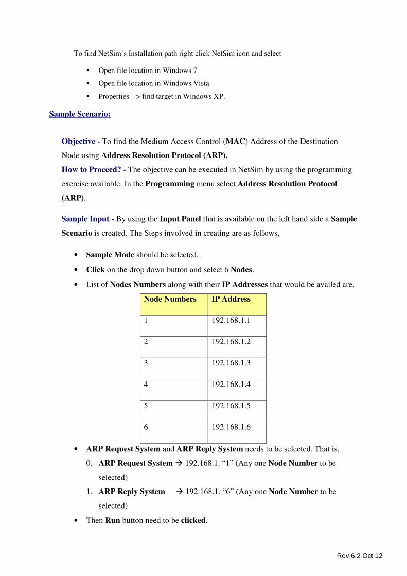
To find NetSim’s Installation path right click NetSim icon and select
� Open file location in Windows 7
� Open file location in Windows Vista
� Properties --> find target in Windows XP.
Sample Scenario:
Objective - To find the Medium Access Control (MAC) Address of the Destination
Node using Address Resolution Protocol (ARP).
How to Proceed? - The objective can be executed in NetSim by using the programming
exercise available. In the Programming menu select Address Resolution Protocol
(ARP).
Sample Input - By using the Input Panel that is available on the left hand side a Sample
Scenario is created. The Steps involved in creating are as follows,
• Sample Mode should be selected.
• Click on the drop down button and select 6 Nodes.
• List of Nodes Numbers along with their IP Addresses that would be availed are,
Node Numbers IP Address
1 192.168.1.1
2 192.168.1.2
3 192.168.1.3
4 192.168.1.4
5 192.168.1.5
6 192.168.1.6
• ARP Request System and ARP Reply System needs to be selected. That is,
0. ARP Request System � 192.168.1. “1” (Any one Node Number to be
selected)
1. ARP Reply System � 192.168.1. “6” (Any one Node Number to be
selected)
• Then Run button need to be clicked.
Rev 6.2 Oct 12
Output - Output for the above Sample is as follows,
• The Source Node (i.e. Node Number 1 in the above example) sends the ARP
Request to the Connecting Device.
• The Connecting Device then broadcasts the ARP Request to all the Nodes
available in the network.
• The Destination Node (i.e. Node Number 6 in the above example) sends an
acknowledgement in the form of ARP Reply (i.e. The Destination MAC -
MAC Address of the Destination Node) to the Connecting Device.
• The Device then transmits the ARP Reply (i.e. The Destination MAC - MAC
Address of the Destination Node) only to the Source Node.
• Once the sample experiment is done, then Refresh button can be clicked to
create new samples.
Assignment of Sites to Concentrator
Programming Guidelines
This section guides the user to link his/her own code for Assignment of Sites to Concentrator
to NetSim.
Pre - Conditions
The user program should read the inputted scenario from text file named ‘Input’ with
extension txt.
The user program after executing the concept should write the required output to a file
named ‘Output’ with extension txt.
Note:
The temporary directory is navigated through the following step.
run ���� Type "%temp%" ���� NetSim ���� "Input.txt" and "Output.txt"
General Program Flow
The program begins with the Reading of the Inputs from the input file Input.txt.
Executing the required concept and,
The results of the program should be written into the output file Output.txt.
Rev 6.2 Oct 12
Input file format
Input.txt contains the number of sites, number of concentrators, and number of sites
that can be assigned to a concentrator, the order in which sites are to be assigned and
the distance matrix given by the user. The format of input.txt is:
Number_of_Sites=2
Number_of_Concentrators=2
Sites_per_Concentrator=1
Selected_Priority=1>0>
Distance
1>2>
3>4>
Note: ‘>’ is the delimiter symbol, which is used to separate each input.
Output file format
In the output file (i.e. ‘Output.txt’) each line should indicate one complete traverse.
For example, for the above input, the output file should be:
2>1>
1>2>
In each line, the first character indicates the site and the rest indicates the
concentrators. The second character (excluding the ‘>’ symbol) is the first
concentrator found with minimum distance/cost. The third character is a
concentrator, which has the minimum distance/cost compared to the previous one
and so on.
Note: ‘>’ is the delimiter symbol, which is used to separate each input.
Interface Source Code
Interface Source code code written in C is given using this the user can write only the
Assignments of Sites to Concentrators inside the function fnAssignmentsofSites()
using the variables already declared.
To view the interface source code, go to
NetSim Installation path / src / Programming/ AssignSites.c
To find NetSim’s Installation path right click NetSim icon and select
� Open file location in Windows 7
� Open file location in Windows Vista
Rev 6.2 Oct 12

� Properties --> find target in Windows XP.
Sample Scenarios:
Objective - To allocate the resource which is concentrator to the require system which is
sites based on the distance for each sites to concentrator.
How to proceed? - The objective can be executed in NetSim using the programming exercise
available, under programming user has to select Assignment of Sites to Concentrator.
Sample Input - By using the Input Panel that is available on the left hand side a Sample
Scenario is created. The Steps involved in creating are as follows,
• Sample Mode should be selected.
• Number of Sites need to be selected. The value that has selected ranges from 1 to
7.
• Number of Concentrators need to be selected. The values available for selection
are 2, 3 and 4.
• Number of Sites / Concentrators need to be selected. The value that has selected
ranges from 1 to 7.
• Click on the image to select Priority. Click on Change Priority to reset the
Priority of the Sites.
• Enter the Distance in the given table. Distance should be in the range, 1 to 99 km.
• Then Run button need to be clicked. Refresh button can be used if new Inputs
have to be given.
• Click on Concept, Algorithm, Pseudo Code & Flow Chart to get help on it.
Output - The following steps are under gone internally,
• The site which has the highest priority searches for a concentrator which is the
nearest.
• A red line appears between the site and a concentrator. This indicates the only
shortest path available between the site and the concentrators. Hence, it
indicates the site has been allocated to that concentrator.
• A site can have only one concentrator, whereas a concentrator can have many
sites linked to it.
• Once the sample experiment is done, then Refresh button can be clicked to
create New Samples.
Rev 6.2 Oct 12
Cryptography - Substitution - Encryption
Programming Guidelines
This section guides the user to link his/her own code for Substitution to NetSim.
Pre-conditions
The user program should read the inputted scenario from text file named ‘Input’ with
extension txt.
The user program after executing the concept should write the required output to a file
named ‘Output’ with extension txt.
Note:
The temporary directory is navigated through the following step.
run ���� Type "%temp%" ���� NetSim ���� "Input.txt" and "Output.txt"
General Program Flow
The program begins with the Reading of the Inputs from the input file Input.txt.
Executing the required concept and, the results of the program should be written into
the output file Output.txt.
Input File Format
There are six lines in Input.txt file.
Cryptographic_Technique=Substitution
Cryptographic_Method=Encryption
Plain_Text:
tetcos
Key_Text:
2
Output File Format
Plain letter>encrypted letter for the corresponding plain letter>
t>u>v>
e>f>g>
t>u>v>
c>d>e>
o>p>q>
s>t>u>
Rev 6.2 Oct 12
Interface Source Code
Interface Source code written in C is given using this the user can write only the Substitution-
Encryption inside the function fnSubstutionEncryption () using the variables already
declared.
To view the interface source code, go to
NetSim Installation path / src / Programming/ SubstEncrypt.c
To find NetSim’s Installation path right click NetSim icon and select
� Open file location in Windows 7
� Open file location in Windows Vista
� Properties --> find target in Windows XP.
Cryptography - Substitution - Decryption
Programming Guidelines
This section guides the user to link his/her own code for Substitution to NetSim.
Pre - Conditions
The user program should read the inputted scenario from text file named ‘Input’ with
extension txt.
The user program after executing the concept should write the required output to a file
named ‘Output’ with extension txt.
Note:
The temporary directory is navigated through the following step.
run ���� Type "%temp%" ���� NetSim ���� "Input.txt" and "Output.txt"
General Program Flow
The program begins with the Reading of the Inputs from the input file Input.txt.
Executing the required concept and,
The results of the program should be written into the output file Output.txt.
Input File Format
There are six lines in Input.txt file.
Cryptographic_Technique=Substitution
Cryptographic_Method=Decryption
Cipher_Text:
vgvequ
Key_Text:
2
Rev 6.2 Oct 12
Output File Format
Cipher letter>decrypted letter for the corresponding cipher letter>
v>u>t>
g>f>e>
v>u>t>
e>d>c>
q>p>o>
u>t>s>
Interface Source Code
Interface Source code written in C is given using this the user can write only the Substitution-
Decryption inside the function SubstutionDecryption () using the variables already declared.
To view the interface source code, go to
NetSim Installation path / src / Programming/ SubstDecrypt.c
To find NetSim’s Installation path right click NetSim icon and select
� Open file location in Windows 7
� Open file location in Windows Vista
� Properties --> find target in Windows XP.
Sample Scenarios:
Objective - Encrypt and decrypt the message with the same key value using Substitution.
How to Proceed? - The objective can be executed in NetSim using the programming
exercise available. Under programming user has to select Cryptography ���� Substitution.
� Encryption:
Sample Input: In the Input panel the following steps need to be done,
• Sample Mode should be selected.
• Encryption need to be selected.
• Enter the Plain Text that needs to be encrypted. Maximum of 8 alphabets need
to be entered.
• Enter the Key Value. This is an Integer which is within the range 0 to 26.
• Then Run button need to be clicked. Refresh button can be used if new
Inputs have to be given.
Output - The following steps are under gone internally,
• The Plain Text and Key Value entered would be displayed in red color.
• The corresponding Cipher Text would be obtained.
• Once the sample experiment is done, then Refresh button can be clicked to
create New Samples.
Rev 6.2 Oct 12
� Decryption:
Sample Input: In the Input panel the following steps need to be done,
• Sample Mode should be selected.
• Decryption need to be selected.
• Cipher Text obtained while encryption is filled in the Plain Text and also the
Key Text is same as that entered while encrypting.
• Then Run button need to be clicked. Refresh button can be used if new
Inputs have to be given.
Output - The following steps are under gone internally,
• The Cipher Text and Key Value entered would be displayed in red color.
• The corresponding Plain Text that had been entered at the time of encrypting is
obtained.
• Once the sample experiment is done, then Refresh button can be clicked to
create New Samples.
Cryptography - Transposition - Encryption
Programming Guidelines
This section guides the user to link his/her own code for Transposition Encryption to NetSim.
Pre-conditions
The user program should read the inputted scenario from text file named ‘Input’ with
extension txt.
The user program after executing the concept should write the required output to a file
named ‘Output’ with extension txt.
Note:
The temporary directory is navigated through the following step.
run ���� Type "%temp%" ���� NetSim ���� "Input.txt" and "Output.txt"
General Program Flow
The program begins with the Reading of the Inputs from the input file Input.txt.
Executing the required concept and,
The results of the program should be written into the output file Output.txt.
Input File Format
Cryptographic_Technique=Transposition
Rev 6.2 Oct 12
Cryptographic_Method=Encryption
Plain_Text:
TETCOS
Key_Text:
BLORE
Output File Format
1>3>4>5>2>
T>E>T>C>O>S>T>E>T>C>
T>S>O>C>E>T>T>E>C>T>
Interface Source Code
Interface Source code written in C is given using this the user can write only the
Transposition-Encryption inside the function fnTranspositionEncryption() using the variables
already declared.
To view the interface source code, go to
NetSim Installation path / src / Programming/ TranspEncrypt.c
To find NetSim’s Installation path right click NetSim icon and select
� Open file location in Windows 7
� Open file location in Windows Vista
� Properties --> find target in Windows XP.
Cryptography - Transposition – Decryption
Programming Guidelines
This section guides the user to link his/her own code for Transposition Decryption to NetSim.
Pre - Conditions
The user program should read the inputted scenario from text file named ‘Input’ with
extension txt.
The user program after executing the concept should write the required output to a file
named ‘Output’ with extension txt.
Note:
The temporary directory is navigated through the following step.
run ���� Type "%temp%" ���� NetSim ���� "Input.txt" and "Output.txt"
Rev 6.2 Oct 12
General Program Flow
The program begins with the Reading of the Inputs from the input file Input.txt.
Executing the required concept and,
The results of the program should be written into the output file Output.txt.
Input File Format
Cryptographic_Technique=Transposition
Cryptographic_Method=Decryption
Cipher_Text:
TSOCETTECT
Key_Text:
BLORE
Output File Format
BELOR>
1>5>2>3>4>
T>O>E>T>C>S>C>T>E>T>
Interface Source Code
Interface Source code written in C is given using this the user can write only the
Transposition-Decryption inside the function fnTranspositionDecryption() using the variables
already declared.
To view the interface source code, go to
NetSim Installation path / src / Programming/ TranspDecrypt.c
To find NetSim’s Installation path right click NetSim icon and select
� Open file location in Windows 7
� Open file location in Windows Vista
� Properties --> find target in Windows XP.
Sample Scenarios:
Objective - Encrypt and decrypt the message with the same key text using Transposition.
How to Proceed? - The objective can be executed in NetSim using the programming
exercise available. Under programming user has to select Cryptography ���� Transposition.
� Encryption:
Sample Input: In the Input panel the following steps need to be done,
• Sample Mode should be selected.
• Encryption need to be selected.
Rev 6.2 Oct 12
• Enter the Cipher Text. Maximum of 14 Characters can be entered.
• Enter the Key Value. Maximum of 8 alphabets can be entered.
• Then Run button need to be clicked. Refresh button can be used if new
Inputs have to be given.
Output - The following steps are under gone internally,
• The entered Key Value would be displayed first.
• The order of the Key Value is internally sensed.
• The corresponding Cipher Text is obtained.
• Once the sample experiment is done, then Refresh button can be clicked
to create New Samples.
� Decryption:
Sample Input: In the Input panel the following steps need to be done,
• Once Encryption is done Decryption has to be selected.
• The Cipher Text obtained for Encryption is the Cipher Text for
Decryption. This would be automatically taken. Maximum of 14
Characters can be entered.
• Enter the Key Value will also be taken internally. Maximum of 8 alphabets
can be entered.
• Then Run button need to be clicked. Refresh button can be used if new
Inputs have to be given.
Output - The following steps are under gone internally,
• The entered Key Value would be displayed first. This is arranged in such a
way that the order is changed when compared to Encryption.
• The order of the Key Value is internally sensed.
• The corresponding Plain Text is obtained. This Plain Text would be
similar to the Plain Text entered at the time of Encryption.
• Once the sample experiment is done, then Refresh button can be clicked
to create New Samples.
Cryptography - XOR - Encryption
Programming Guidelines
This section guides the user to link his/her own code for XOR Encryption to NetSim.
Pre - Conditions
The user program should read the inputted scenario from text file named ‘Input’ with
extension txt.
Rev 6.2 Oct 12
The user program after executing the concept should write the required output to a file
named ‘Output’ with extension txt.
Note:
The temporary directory is navigated through the following step.
run ���� Type "%temp%" ���� NetSim ���� "Input.txt" and "Output.txt"
General Program Flow
The program begins with the Reading of the Inputs from the input file Input.txt.
Executing the required concept and,
The results of the program should be written into the output file Output.txt.
Input File Format
Cryptographic_Technique=XOR
Cryptographic_Method=Encryption
Plain_Text:
TETCOS
Key_Text:
BNLORE
Output File Format
01010100>01000010>00010110>
01000101>01001110>00001011>
01010100>01001100>00011000>
01000011>01001111>00001100>
01001111>01010010>00011101>
01010011>01000101>00010110>
Interface Source Code
Interface Source code written in C is given using this the user can write only the XOR-
Encryption inside the function fnXOREncryption () using the variables already declared.
To view the interface source code, go to
NetSim Installation path / src / Programming/ XorEncrypt.c
To find NetSim’s Installation path right click NetSim icon and select
� Open file location in Windows 7
� Open file location in Windows Vista
� Properties --> find target in Windows XP.
Rev 6.2 Oct 12
Cryptography - XOR - Decryption
Programming Guidelines
This section guides the user to link his/her own code for XOR Decryption to NetSim.
Pre - Conditions
The user program should read the inputted scenario from text file named ‘Input’ with
extension txt.
The user program after executing the concept should write the required output to a file
named ‘Output’ with extension txt.
Note:
The temporary directory is navigated through the following step.
run � Type "%temp%" � NetSim � "Input.txt" and "Output.txt"
General Program Flow
The program begins with the Reading of the Inputs from the input file Input.txt.
Executing the required concept and,
The results of the program should be written into the output file Output.txt.
Input File Format
Cryptographic_Technique=XOR
Cryptographic_Method=Decryption
Cipher_Text:
000101100000101100011000000011000001110100010110
Key_Text:
BNLORE
Output File Format
00010110>01000010>01010100>
00001011>01001110>01000101>
00011000>01001100>01010100>
00001100>01001111>01000011>
00011101>01010010>01001111>
00010110>01000101>01010011>
Interface Source Code
Here a skeleton code written in C is given using this the user can write only the XOR-
Decryption inside the function fnXORDecryption () using the variables already declared.
To view the interface source code, go to
NetSim Installation path / src / Programming/ XorDecrypt.c
Rev 6.2 Oct 12
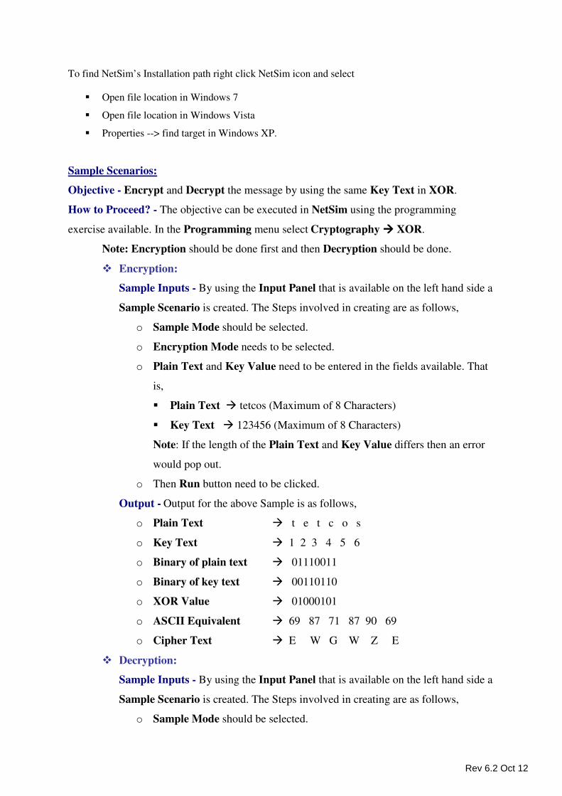
To find NetSim’s Installation path right click NetSim icon and select
� Open file location in Windows 7
� Open file location in Windows Vista
� Properties --> find target in Windows XP.
Sample Scenarios:
Objective - Encrypt and Decrypt the message by using the same Key Text in XOR.
How to Proceed? - The objective can be executed in NetSim using the programming
exercise available. In the Programming menu select Cryptography ���� XOR.
Note: Encryption should be done first and then Decryption should be done.
� Encryption:
Sample Inputs - By using the Input Panel that is available on the left hand side a
Sample Scenario is created. The Steps involved in creating are as follows,
o Sample Mode should be selected.
o Encryption Mode needs to be selected.
o Plain Text and Key Value need to be entered in the fields available. That
is,
� Plain Text � tetcos (Maximum of 8 Characters)
� Key Text � 123456 (Maximum of 8 Characters)
Note: If the length of the Plain Text and Key Value differs then an error
would pop out.
o Then Run button need to be clicked.
Output - Output for the above Sample is as follows,
o Plain Text � t e t c o s
o Key Text � 1 2 3 4 5 6
o Binary of plain text � 01110011
o Binary of key text � 00110110
o XOR Value � 01000101
o ASCII Equivalent � 69 87 71 87 90 69
o Cipher Text � E W G W Z E
� Decryption:
Sample Inputs - By using the Input Panel that is available on the left hand side a
Sample Scenario is created. The Steps involved in creating are as follows,
o Sample Mode should be selected.
Rev 6.2 Oct 12
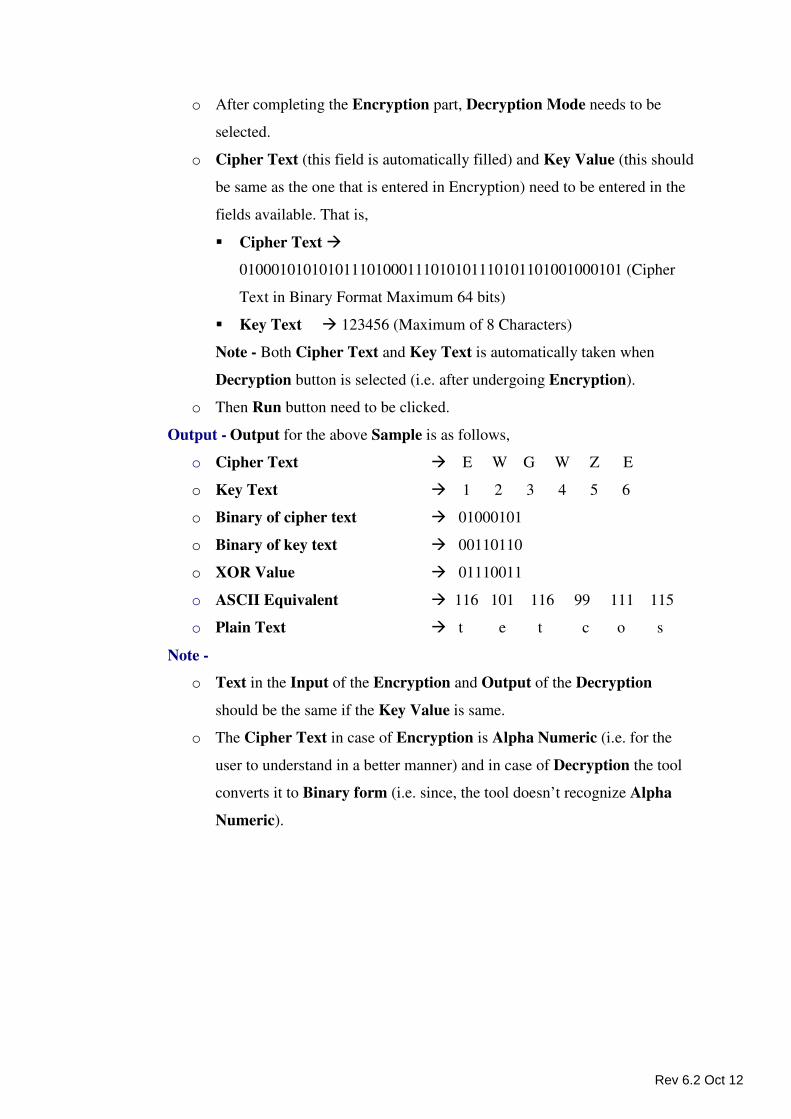
o After completing the Encryption part, Decryption Mode needs to be
selected.
o Cipher Text (this field is automatically filled) and Key Value (this should
be same as the one that is entered in Encryption) need to be entered in the
fields available. That is,
� Cipher Text �
010001010101011101000111010101110101101001000101 (Cipher
Text in Binary Format Maximum 64 bits)
� Key Text � 123456 (Maximum of 8 Characters)
Note - Both Cipher Text and Key Text is automatically taken when
Decryption button is selected (i.e. after undergoing Encryption).
o Then Run button need to be clicked.
Output - Output for the above Sample is as follows,
o Cipher Text � E W G W Z E
o Key Text � 1 2 3 4 5 6
o Binary of cipher text � 01000101
o Binary of key text � 00110110
o XOR Value � 01110011
o ASCII Equivalent � 116 101 116 99 111 115
o Plain Text � t e t c o s
Note -
o Text in the Input of the Encryption and Output of the Decryption
should be the same if the Key Value is same.
o The Cipher Text in case of Encryption is Alpha Numeric (i.e. for the
user to understand in a better manner) and in case of Decryption the tool
converts it to Binary form (i.e. since, the tool doesn’t recognize Alpha
Numeric).
Rev 6.2 Oct 12
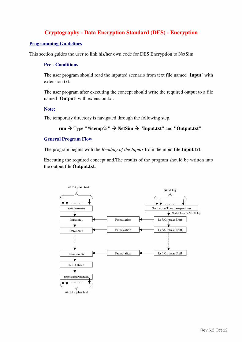
Cryptography - Data Encryption Standard (DES) - Encryption
Programming Guidelines
This section guides the user to link his/her own code for DES Encryption to NetSim.
Pre - Conditions
The user program should read the inputted scenario from text file named ‘Input’ with
extension txt.
The user program after executing the concept should write the required output to a file
named ‘Output’ with extension txt.
Note:
The temporary directory is navigated through the following step.
run ���� Type "%temp%" ���� NetSim ���� "Input.txt" and "Output.txt"
General Program Flow
The program begins with the Reading of the Inputs from the input file Input.txt.
Executing the required concept and,The results of the program should be written into
the output file Output.txt.
Rev 6.2 Oct 12
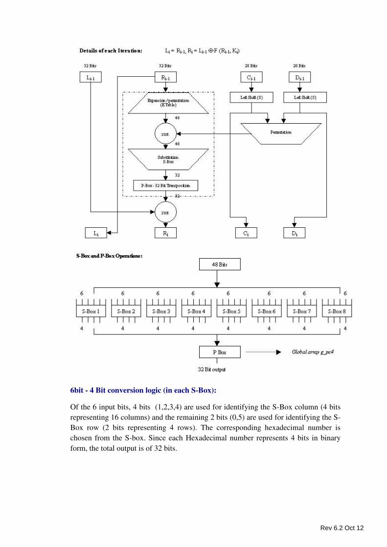
6bit - 4 Bit conversion logic (in each S-Box):
Of the 6 input bits, 4 bits (1,2,3,4) are used for identifying the S-Box column (4 bits
representing 16 columns) and the remaining 2 bits (0,5) are used for identifying the S-
Box row (2 bits representing 4 rows). The corresponding hexadecimal number is
chosen from the S-box. Since each Hexadecimal number represents 4 bits in binary
form, the total output is of 32 bits.
Rev 6.2 Oct 12
Input File Format
Cryptographic_Method=Encryption
Key_Text=abcdef1234567890
No_of_Iterations=1
Data=tetcos
Output File Format
The number of lines present depends on the number of iterations chosen. The number
of lines equals the number of iterations, plus one. The last line of inputs gives the data
(encrypted data if encryption has been chosen, else the decrypted data
if decryption has been chosen). The previous lines give the DES Key generated for
encryption or decryption.
110101010111110010011010110000101110011000011001
616075733F724B40
Interface Source Code
Interface Source code written in C is given using this the user can write only the DES-
Encryption inside the function fnDESEncryption() using the variables already declared.
To view the interface source code, go to
NetSim Installation path / src / Programming/ DesEncrypt.c
To find NetSim’s Installation path right click NetSim icon and select
� Open file location in Windows 7
� Open file location in Windows Vista
� Properties --> find target in Windows XP.
Cryptography - Data Encryption Standard (DES) - Decryption
Programming Guidelines
This section guides the user to link his/her own code for DES Decryption to NetSim.
Pre - Conditions
The user program should read the inputted scenario from text file named ‘Input’ with
extension txt.
The user program after executing the concept should write the required output to a file
named ‘Output’ with extension txt.
Rev 6.2 Oct 12
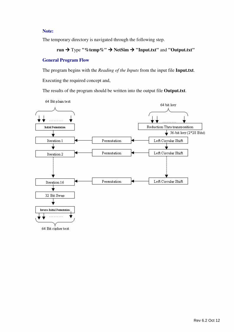
Note:
The temporary directory is navigated through the following step.
run ���� Type "%temp%" ���� NetSim ���� "Input.txt" and "Output.txt"
General Program Flow
The program begins with the Reading of the Inputs from the input file Input.txt.
Executing the required concept and,
The results of the program should be written into the output file Output.txt.
Rev 6.2 Oct 12
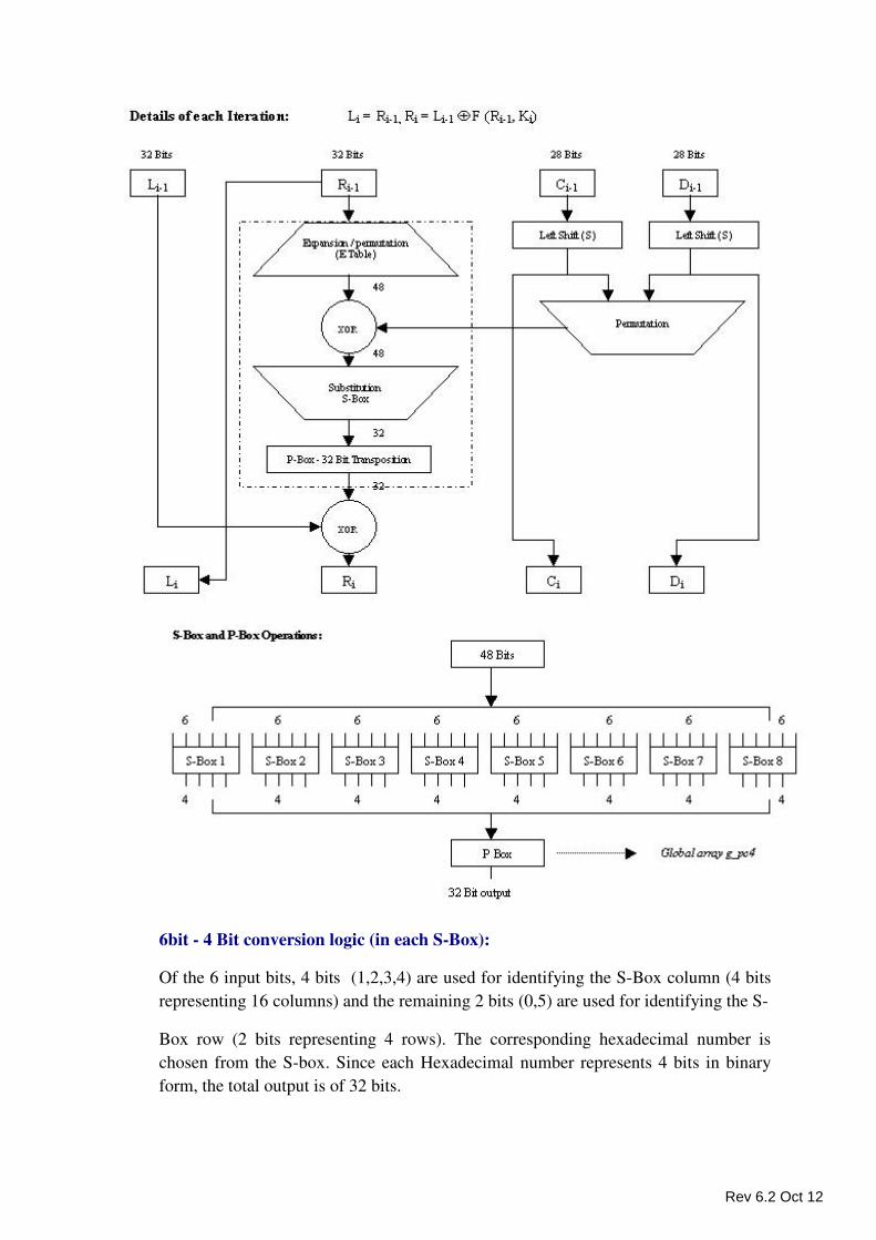
6bit - 4 Bit conversion logic (in each S-Box):
Of the 6 input bits, 4 bits (1,2,3,4) are used for identifying the S-Box column (4 bits
representing 16 columns) and the remaining 2 bits (0,5) are used for identifying the S-
Box row (2 bits representing 4 rows). The corresponding hexadecimal number is
chosen from the S-box. Since each Hexadecimal number represents 4 bits in binary
form, the total output is of 32 bits.
Rev 6.2 Oct 12
Input File Format
Cryptographic_Method=Decryption
Key_Text=abcdef1234567890
No_of_Iterations=1
Data=616075733F724B40
Output File Format
The number of lines present depends on the number of iterations chosen. The number
of lines equals the number of iterations, plus one. The last line of inputs gives the data
(encrypted data if encryption has been chosen, else the decrypted data if decryption has been
chosen). The previous lines give the DES Key generated for encryption or decryption.
110101010111110010011010110000101110011000011001
tetcos
Interface Source Code
Interface Source code written in C is given using this the user can write only the DES-
Decryption inside the function fnDESDecryption () using the variables already declared.
To view the interface source code, go to
NetSim Installation path / src / Programming/ DesDecrypt.c
To find NetSim’s Installation path right click NetSim icon and select
� Open file location in Windows 7
� Open file location in Windows Vista
� Properties --> find target in Windows XP.
Sample Scenarios:
Objective - Encrypt and decrypt the message with the using DES.
How to Proceed? - The objective can be executed in NetSim using the programming
exercise available. Under programming user has to select Cryptography � Advanced �
Data Encryption Standard.
� Encryption:
Sample Inputs - In the Input panel the following steps need to be done,
• Sample Mode should be selected.
• Encryption need to be selected.
• Enter the Key Text in the provided field. Only hexadecimal characters
have to be entered. Maximum of 16 characters can be entered in this field.
Characters more than 16 will be filled in the Data field.
Rev 6.2 Oct 12
• Number of Iterations need to be selected. The value ranges from 1 to 16.
• Data needs to be entered in this field that has to be encrypted. Data can be
entered only when the Enter Key Text field is filed with 16 hexadecimal
characters. Maximum of 1500 characters can be stuffed into this field.
• Then Run button need to be clicked. Refresh button can be used if new
Inputs have to be given.
Output -
• Key1 (i.e. if Iteration is 1) in binary format is obtained.
• The corresponding Cipher text is obtained.
• Click on Copy button and then on the Paste button to make use of the
Cipher text for Decryption.
• Once the sample experiment is done, then Refresh button can be clicked
to create New Samples.
� Decryption:
Sample Inputs - In the Input panel the following steps need to be done,
• Sample Mode should be selected.
• Once the Encryption is done, click on Copy and Paste buttons. The
encrypted data is filled in the data field available in the Decryption view.
• Fields such as Enter the Key Text, Number of Iteration and Data is filled
in automatically when Copy and Paste button is clicked.
• Then Run button need to be clicked. Refresh button can be used if new
Inputs have to be given.
Output - The following steps are under gone internally,
• Key1 (i.e. if Iteration is 1) in binary format is obtained.
• The Data that was entered in the Encryption view would be encrypted and
displayed.
• Once the sample experiment is done, then Refresh button can be clicked
to create New Samples.
Rivest-Shamir - Adleman Algorithm (RSA)
Programming Guidelines
This section guides the user to link his/her own code for RSA Algorithm to NetSim.
Pre - Conditions
The user program should read the inputted scenario from text file named ‘Input’ with
extension txt.
Rev 6.2 Oct 12
The user program after executing the concept should write the required output to a file
named ‘Output’ with extension txt.
The path of the input file and the output file can be viewed on clicking the Button
“Path” in NetSim.
Note:
The temporary directory is navigated through the following step.
run ���� Type "%temp%" ���� NetSim ���� "Input.txt" and "Output.txt"
General Program Flow
The program begins with the Reading of the Inputs from the input file Input.txt.
Executing the required concept and,
The results of the program should be written into the output file Output.txt.
Input file format
Input.txt file has the input data. The format is:
Plain_Text=T
Output file format
Output.txt file has the following line format:
dt1>dt2>dt3>dt4>dt5>dt6>dt7>dt8> dt 1: specifies the prime P
dt 2: specifies the prime Q
dt 3: specifies the value of N
dt 4: specifies the value of Z
dt 5: specifies the value of Kp
dt 6: specifies the value of Ks
dt 7: specifies the value of the Cipher Text
dt 8: specifies the value of the Plain Text
Example:
For input: ‘T’
Output: 11>3>33>20>7>3>14>20>
Interface Source Code
To view the interface source code, go to
NetSim Installation path / src / Programming/ RSA.c
To find NetSim’s Installation path right click NetSim icon and select
� Open file location in Windows 7
Rev 6.2 Oct 12
� Open file location in Windows Vista
� Properties --> find target in Windows XP.
Sample Scenario:
Objective - Encrypt and decrypt the message with the using DES.
How to Proceed? - The objective can be executed in NetSim using the programming
exercise available. Under programming user has to select Cryptography � Advanced �
RSA.
Sample Inputs - In the Input panel the following steps need to be done,
• Sample Mode should be selected.
• Plain Text of only one character has to be entered in the field available.
• Then Run button need to be clicked. Refresh button can be used if new
Inputs have to be given.
Output - The following steps are under gone internally,
• Value of the prime numbers P and Q are obtained.
• Value of N[p*q] is obtained.
• Value of Z [(p-1)*(q-1)] is obtained.
• Value of Kp and Ks is obtained
• Plain Text which is the actual count of the alphabet is obtained.
• The corresponding Cipher Text is obtained.
• Once the sample experiment is done, then Refresh button can be clicked to
create New Samples.
Cryptography - Wired Equivalent Privacy (WEP) – Encryption
Programming Guidelines
This section guides the user to link his/her own code for WEP Encryption to NetSim.
Pre - Conditions
The user program should read the inputted scenario from text file named ‘Input’ with
extension txt.
The user program after executing the concept should write the required output to a file
named ‘Output’ with extension txt.
Note:
The temporary directory is navigated through the following step.
run ���� Type "%temp%" ���� NetSim ���� "Input.txt" and "Output.txt"
Rev 6.2 Oct 12
General Program Flow
The program begins with the Reading of the Inputs from the input file Input.txt.
Executing the required concept and,
The results of the program should be written into the output file Output.txt.
Input File Format
Cryptographic_Method=Encryption
Data:
TETCOS
Output File Format
There are 3 lines in output.txt file
Initialization Vector
Key Text
Cipher Text
Ex:
8A699C
0123456789
364130B9CA018D5B760383CD85528751
Interface Source Code
Interface Source code written in C is given using this the user can write only the WEP-
Encryption inside the function fnWEPEncrypt () using the variables already declared.
To view the interface source code, go to
NetSim Installation path / src / Programming/ WEPEncrypt.c
To find NetSim’s Installation path right click NetSim icon and select
� Open file location in Windows 7
� Open file location in Windows Vista
� Properties --> find target in Windows XP.
Cryptography - Wired Equivalent Privacy (WEP) - Decryption
Programming Guidelines
This section guides the user to link his/her own code for WEP Decryption to NetSim.
Pre - Conditions
The user program should read the inputted scenario from text file named ‘Input’ with
extension txt.
Rev 6.2 Oct 12
The user program after executing the concept should write the required output to a file
named ‘Output’ with extension txt.
Note:
The temporary directory is navigated through the following step.
run ���� Type "%temp%" ���� NetSim ���� "Input.txt" and "Output.txt"
General Program Flow
The program begins with the Reading of the Inputs from the input file Input.txt.
Executing the required concept and,
The results of the program should be written into the output file Output.txt.
Input File Format
Cryptographic_Method=Decryption
Initialization_Vector=8A699C
Key=0123456789
Data:
364130B9CA018D5B760383CD85528751
Output File Format
Plain text
Ex:
TETCOS
Interface Source Code
Interface Source code written in C is given using this the user can write only the
WEP-Decryption inside the function fnWEPDecrypt () using the variables already
declared.
To view the interface source code, go to
NetSim Installation path / src / Programming/ WEPDecrypt.c
To find NetSim’s Installation path right click NetSim icon and select
� Open file location in Windows 7
� Open file location in Windows Vista
� Properties --> find target in Windows XP.
Rev 6.2 Oct 12
Sample Scenarios:
Objective - Encrypt and Decrypt the message by using WEP.
How to Proceed? - The objective can be executed in NetSim using the programming
exercise available. In Programming menu select Cryptography � Advanced � Wired
Equivalent Privacy.
Note: Encryption should be done first and then Decryption should be done.
� Encryption
Sample Inputs - By using the Input Panel that is available on the left hand side a
Sample Scenario is created. The Steps involved in creating are as follows,
o Sample Mode should be selected.
o Under Cryptographic Method, Encryption Mode needs to be selected.
o Input � Data (Maximum of 1500 Characters) - NetSim TetCos
Bangalore
o Then Run button need to be clicked.
Sample Output - Output for the above Sample is as follows,
o Initialization Vector : 3E41C6
o Key : ABCDEF0123
o The Encrypted Text obtained -
“786441A955C419F9537576954F897BCC5866549653DB5CA73E1B4D
F63CA939AD”
o Click on Copy button and then on Paste button. This would Copy the
Encrypted Text onto the Decryption Input Data field.
� Decryption
Sample Inputs - By using the Input Panel that is available on the left hand side
a Sample Scenario is created. The Steps involved in creating are as follows,
o Sample Mode should be selected. (This is Automatically selected once
the Paste button is clicked at the time of Encrypting the Data).
o Under Cryptographic Method, Encryption Mode needs to be selected.
(This is Automatically selected once the Paste button is clicked at the
time of Encrypting the Data).
o Enter Key Value � 3E41C6ABCDEF0123 (16Hexadecimal Characters).
(This field is Automatically filled once the Paste button is clicked at the
time of Encrypting the Data).
Rev 6.2 Oct 12
o Number of Iterations � 1.
o Input � Data -
“786441A955C419F9537576954F897BCC5866549653DB5CA73E1B4D
F63CA939AD” (This field is Automatically filled once the Paste button
is clicked at the time of Encrypting the Data).
o Then Run button need to be clicked.
Sample Output - Output for the above Sample is as follows,
o Initialization Vector : 3E41C6
o Key : ABCDEF0123
o The Encrypted Text obtained - NetSim TetCos Bangalore
Distance Vector Routing
Programming Guidelines
This section guides the user to link his/her own code for Distance Vector Routing to NetSim.
Pre - Conditions
The user program should read the input scenario from text file named ‘Input’ with
extension txt.
The user program after executing the concept should write the required output to a file
named ‘Output’ with extension txt.
Note:
The temporary directory is navigated through the following step.
run ���� Type "%temp%" ���� NetSim ���� "Input.txt" and "Output.txt"
General Program Flow
The program begins with the Reading of the Inputs from the input file Input.txt.
Executing the required concept and
The results of the program should be written into the output file Output.txt.
Input File Format
Router_ID=1>Router_Name=Router_1>No_Of_Neighbour=2>Neighbours_ID=2>5
Router_ID=2>Router_Name=Router_2>No_Of_Neighbour=1>Neighbours_ID=1
Router_ID=3>Router_Name=Router_3>No_Of_Neighbour=0
Router_ID=4>Router_Name=Router_4>No_Of_Neighbour=0
Router_ID=5>Router_Name=Router_5>No_Of_Neighbour=1>Neighbours_ID=1
Router_ID=6>Router_Name=Router_6>No_Of_Neighbour=0
Rev 6.2 Oct 12
Output File Format
Initial Stage>Source Router ID -1>Destination
RouterID>CostID>Intermediate RouterID
Ex:
0>1>2>1>0
0>1>5>1>0
0>2>1>1>0
0>5>1>1>0
1>1>2>1>0
1>1>5>1>0
1>2>1>1>0
1>2>5>2>1
1>5>1>1>0
1>5>2>2>1
2>1>2>1>0
2>1>5>1>0
2>2>1>1>0
2>2>5>2>1
2>5>1>1>0
2>5>2>2>1
Interface Source Code
Interface Source code written in C is given using this the user can write only the Distance
Vector Routing inside the function fnDistVectAlgorithm() using the variables already
declared.
To view the interface source code, go to
NetSim Installation path / src / Programming/ DVR.c
To find NetSim’s Installation path right click NetSim icon and select
� Open file location in Windows 7
� Open file location in Windows Vista
� Properties --> find target in Windows XP.
Rev 6.2 Oct 12
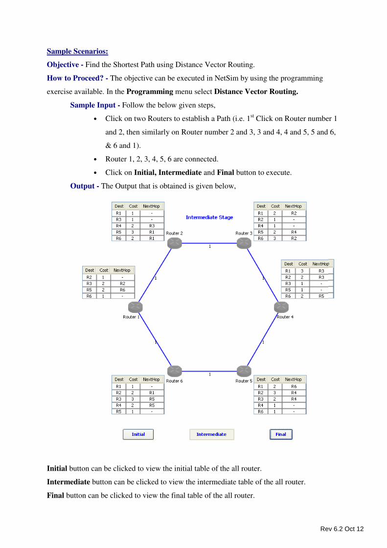
Sample Scenarios:
Objective - Find the Shortest Path using Distance Vector Routing.
How to Proceed? - The objective can be executed in NetSim by using the programming
exercise available. In the Programming menu select Distance Vector Routing.
Sample Input - Follow the below given steps,
• Click on two Routers to establish a Path (i.e. 1st Click on Router number 1
and 2, then similarly on Router number 2 and 3, 3 and 4, 4 and 5, 5 and 6,
& 6 and 1).
• Router 1, 2, 3, 4, 5, 6 are connected.
• Click on Initial, Intermediate and Final button to execute.
Output - The Output that is obtained is given below,
Initial button can be clicked to view the initial table of the all router.
Intermediate button can be clicked to view the intermediate table of the all router.
Final button can be clicked to view the final table of the all router.
Rev 6.2 Oct 12
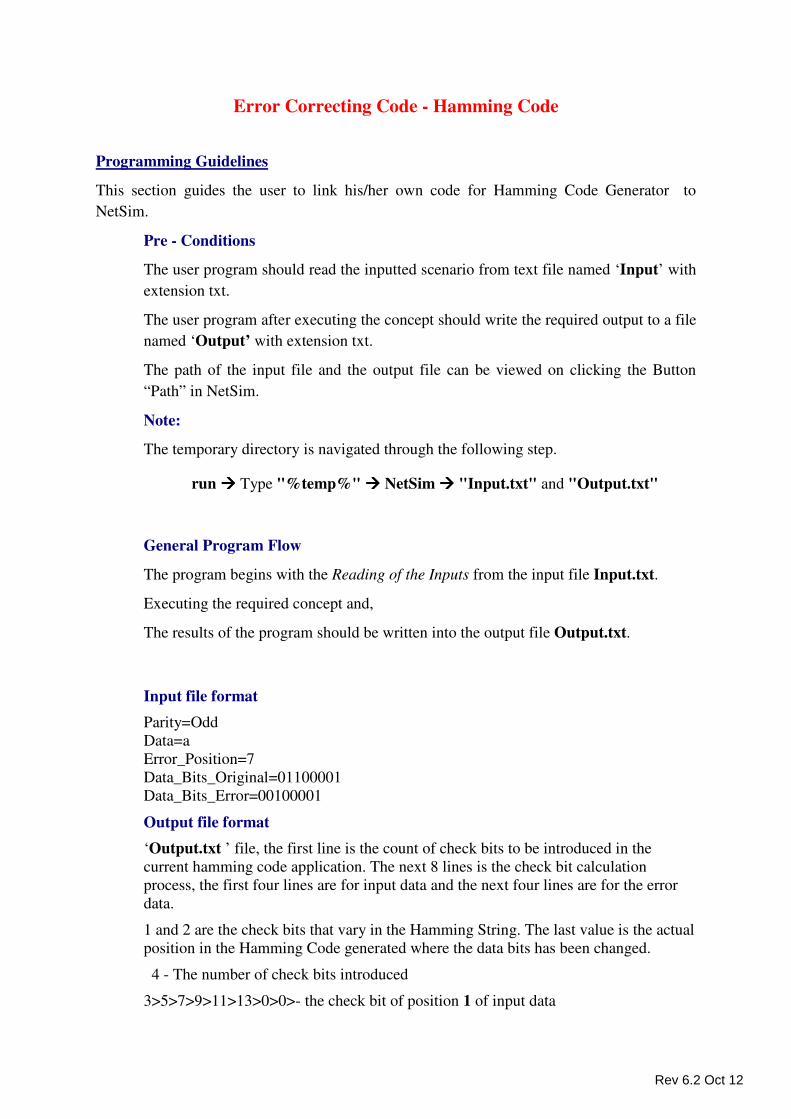
Error Correcting Code - Hamming Code
Programming Guidelines
This section guides the user to link his/her own code for Hamming Code Generator to
NetSim.
Pre - Conditions
The user program should read the inputted scenario from text file named ‘Input’ with
extension txt.
The user program after executing the concept should write the required output to a file
named ‘Output’ with extension txt.
The path of the input file and the output file can be viewed on clicking the Button
“Path” in NetSim.
Note:
The temporary directory is navigated through the following step.
run ���� Type "%temp%" ���� NetSim ���� "Input.txt" and "Output.txt"
General Program Flow
The program begins with the Reading of the Inputs from the input file Input.txt.
Executing the required concept and,
The results of the program should be written into the output file Output.txt.
Input file format
Parity=Odd
Data=a
Error_Position=7
Data_Bits_Original=01100001
Data_Bits_Error=00100001
Output file format
‘Output.txt ’ file, the first line is the count of check bits to be introduced in the
current hamming code application. The next 8 lines is the check bit calculation
process, the first four lines are for input data and the next four lines are for the error
data.
1 and 2 are the check bits that vary in the Hamming String. The last value is the actual
position in the Hamming Code generated where the data bits has been changed.
4 - The number of check bits introduced
3>5>7>9>11>13>0>0>- the check bit of position 1 of input data
Rev 6.2 Oct 12
3>6>7>10>11>1>1>- the check bit of position 2 of input data
5>6>7>12>13>0>0>- the check bit of position 4 of input data
9>10>11>12>13>0>0>- the check bit of position 8 of input data
3>5>7>9>11>13>0>0>- the check bit of position 1 of error data
3>6>7>10>11>1>1>- the check bit of position 2 of error data
5>6>7>12>13>1>1>- the check bit of position 4 of error data
9>10>11>12>13>1>1>- the check bit of position 8 of error data
4>8>12>- the check bit position whose value has been changed and the final error
position.
Interface Source Code
To view the interface source code, go to
NetSim Installation path / src / Programming/ HammingCode.c
To find NetSim’s Installation path right click NetSim icon and select
� Open file location in Windows 7
� Open file location in Windows Vista
� Properties --> find target in Windows XP.
Sample Scenarios:
Objective - To detect and correct the single bit error occurs in the transmission of data.
How to proceed? - The objective can be executed in NetSim using the programming exercise
available, under programming user has to select Error Correcting Code ���� Hamming Code
Sample Inputs - In the Input panel the following steps need to be done,
• Sample Mode should be selected.
• Parity need to be selected. Either Odd or Even can be selected.
• Data need to be entered. Maximum of 8 alphabets can be entered.
• Error Position needs to be selected. Based on the input, its values ranges.
• Then Run button need to be clicked. Refresh button can be used if new
Inputs have to be given.
Output - The following steps are under gone internally,
• Data Bits which if in the binary form is obtained. This Data Bits is obtained for
Original Data entered as well as for the Error selected.
• Depending on the Parity selected, tables of Hamming String, Original Data and
Error Data will be obtained.
Rev 6.2 Oct 12
• For the Error Data table to be obtained click on the Next button available in the
output panel. When the Error Data table is obtained Error Position value is
also obtained.
• Once the sample experiment is done, then Refresh button can be clicked to
create New Samples.
Error Detection Code - Cyclic Redundancy Check (CRC) - 12
Programming Guidelines
This section guides the user to Run his/her own code for Cyclic Redundancy Check to
NetSim.
Pre - Conditions
The user program should read the input scenario from text file named ‘Input’ with
extension txt.
The user program after executing the concept should write the required output to a file
named ‘Output’ with extension txt.
Note:
The temporary directory is navigated through the following step.
run ���� Type "%temp%" ���� NetSim ���� "Input.txt" and "Output.txt"
General Program Flow
The program begins with the Reading of the Inputs from the input file Input.txt.
Executing the required concept and
The results of the program should be written into the output file Output.txt.
Input File Format Algorithm=CRC_12
Condition=No_Error
File_Path=C:\Users\P.Sathishkumar\Documents\1 Th.txt>
Output File format Output contains two values, which is the written in the separate line.
The First line has the CRC value of the data (Sender side CRC value).
The Second line has the CRC value of the data (Receiver side CRC value).
Example: 8CB
000
Rev 6.2 Oct 12
Interface Source Code
Interface Source code written in C is given using this the user can write only the Cyclic
Redundancy Check inside the function fnCRC () using the variables already declared.
To view the interface source code, go to
NetSim Installation path / src / Programming/ Crc12.c
To find NetSim’s Installation path right click NetSim icon and select
� Open file location in Windows 7
� Open file location in Windows Vista
� Properties --> find target in Windows XP.
Sample Scenarios:
Objective - To detect the error found in the file transferred between a Sender and Receiver
using CRC12.
How to Proceed? - The objective can be executed in NetSim using the programming
exercise available. In the Programming Menu select Error Detecting Codes � Cyclic
Redundancy Check.
Sample Input
• For No Error Case - Follow the below given steps,
0. Sample Mode should be selected.
1. Select CRC 12 as Algorithm from the list available.
2. Under Condition, “No Error” should be selected.
3. Under Input, Enter the path of the file name to get its CRC. The file
should be in “.txt” format which should not exceed 5000bytes.
4. Click on Run button to execute. Refresh button can be used if new Inputs
have to be given.
• For Error Case - Follow the below given steps,
0. Sample Mode should be selected.
1. Select CRC 12 as Algorithm from the list available.
2. Under Condition, “Error” should be selected.
3. Under Input, Enter the path of the file name to get its CRC. The file
should be in “.txt” format which should not exceed 5000bytes.
4. Click on Run button to execute. Refresh button can be used if new Inputs
have to be given.
Rev 6.2 Oct 12
Sample Output
• For No Error Case: The Calculated CRC should be Zero when the “.txt file” is
received by the Node2. The message “Data Frame is Flowing from Node1 to
Node2 with No Error”.
• For Error Case: The Calculated CRC should be Non-Zero when the “.txt file”
is received by the Node2. The message “Data Frame is Flowing from Node1 to
Node2 with Error”.
Error Detection Code - Cyclic Redundancy Check (CRC) – 16
Programming Guidelines
This section guides the user to link his/her own code for Cyclic Redundancy Check to
NetSim.
Pre - Conditions
The user program should read the input scenario from text file named ‘Input’ with
extension txt.
The user program after executing the concept should write the required output to a file
named ‘Output’ with extension txt.
Note:
The temporary directory is navigated through the following step.
run ���� Type "%temp%" ���� NetSim ���� "Input.txt" and "Output.txt"
General Program Flow
The program begins with the Reading of the Inputs from the input file Input.txt.
Executing the required concept and
The results of the program should be written into the output file Output.txt.
Input File Format
Algorithm=CRC_16
Condition=No_Error
File_Path=C:\Users\P.Sathishkumar\Documents\1 Th.txt>
Output File format
Output contains two values, which is the written in the separate line.
The First line has the CRC value of the data (Sender side CRC value).
Rev 6.2 Oct 12
The Second line has the CRC value of the data (Receiver side CRC value).
Example:
0FCF
0000
Interface Source Code
Interface Source code written in C is given using this the user can write only the Cyclic
Redundancy Check inside the function fnCRC () using the variables already declared.
To view the interface source code, go to
NetSim Installation path / src / Programming/ Crc16.c
To find NetSim’s Installation path right click NetSim icon and select
� Open file location in Windows 7
� Open file location in Windows Vista
� Properties --> find target in Windows XP.
Sample Scenarios:
Objective - To detect the error found in the file transferred between a Sender and Receiver
using CRC16.
How to Proceed? - The objective can be executed in NetSim using the programming
exercise available. In the Programming menu select Error Detecting Codes � Cyclic
Redundancy Check.
Sample Input
• For No Error Case - Follow the below given steps,
5. Sample Mode should be selected.
6. Select CRC 16 as Algorithm from the list available.
7. Under Condition, “No Error” should be selected.
8. Under Input, Enter the path of the file name to get its CRC. The file
should be in “.txt” format which should not exceed 5000bytes.
9. Click on Run button to execute. Refresh button can be used if new
Inputs have to be given.
• For Error Case - Follow the below given steps,
10. Sample Mode should be selected.
11. Select CRC 16 as Algorithm from the list available.
12. Under Condition, “Error” should be selected.
Rev 6.2 Oct 12
13. Under Input, Enter the path of the file name to get its CRC. The file
should be in “.txt” format which should not exceed 5000bytes.
14. Click on Run button to execute. Refresh button can be used if new
Inputs have to be given.
Sample Output
• For No Error Case: The Calculated CRC should be Zero when the “.txt
file” is received by the Node2. The message “Data Frame is Flowing from
Node1 to Node2 with No Error”.
• For Error Case: The Calculated CRC should be Non-Zero when the “.txt
file” is received by the Node2. The message “Data Frame is Flowing from
Node1 to Node2 with Error”.
Error Detection Code - Cyclic Redundancy Check (CRC) - 32
Programming Guidelines
This section guides the user to link his/her own code for Cyclic Redundancy Check to
NetSim.
Pre - Conditions
The user program should read the input scenario from text file named ‘Input’ with
extension txt.
The user program after executing the concept should write the required output to a file
named ‘Output’ with extension txt.
Note:
The temporary directory is navigated through the following step.
run ���� Type "%temp%" ���� NetSim ���� "Input.txt" and "Output.txt"
General Program Flow
The program begins with the Reading of the Inputs from the input file Input.txt.
Executing the required concept and
The results of the program should be written into the output file Output.txt.
Input File Format
Algorithm=CRC_32
Condition=No_Error
File_Path=C:\Users\P.Sathishkumar\Documents\1 Th.txt>
Rev 6.2 Oct 12
Output File format
Output contains two values, which is the written in the separate line.
The First line has the CRC value of the data (Sender side CRC value).
The Second line has the CRC value of the data (Receiver side CRC value).
Example:
DD8F598B
00000000
Interface Source Code
Interface Source code written in C is given using this the user can write only the
Cyclic Redundancy Check inside the function fnCRC () using the variables already
declared.
To view the interface source code, go to
NetSim Installation path / src / Programming/ Crc32.c
To find NetSim’s Installation path right click NetSim icon and select
� Open file location in Windows 7
� Open file location in Windows Vista
� Properties --> find target in Windows XP.
Sample Scenarios:
Objective - To detect the error found in the file transferred between a Sender and Receiver
using CRC32.
How to Proceed? - The objective can be executed in NetSim using the programming
exercise available. In the Programming menu select Error Detecting Codes �
Cyclic Redundancy Check.
Sample Input
• For No Error Case - Follow the below given steps,
0. Sample Mode should be selected.
1. Select CRC 32 as Algorithm from the list available.
2. Under Condition, “No Error” should be selected.
3. Under Input, Enter the path of the file name to get its CRC. The
file should be in “.txt” format which should not exceed 5000bytes.
4. Click on Run button to execute. Refresh button can be used if new
Inputs have to be given.
• For Error Case - Follow the below given steps,
Rev 6.2 Oct 12
0. Sample Mode should be selected.
1. Select CRC 32 as Algorithm from the list available.
2. Under Condition, “Error” should be selected.
3. Under Input, Enter the path of the file name to get its CRC. The
file should be in “.txt” format which should not exceed 5000bytes.
4. Click on Run button to execute. Refresh button can be used if new
Inputs have to be given.
Sample Output
• For No Error Case: The Calculated CRC should be Zero when the “.txt
file” is received by the Node2. The message “Data Frame is Flowing
from Node1 to Node2 with No Error”.
• For Error Case: The Calculated CRC should be Non-Zero when the
“.txt file” is received by the Node2. The message “Data Frame is
Flowing from Node1 to Node2 with Error”.
Error Detection Code - Cyclic Redundancy Check (CRC) – CCITT
Programming Guidelines
This section guides the user to link his/her own code for Cyclic Redundancy Check to
NetSim.
Pre - Conditions
The user program should read the input scenario from text file named ‘Input’ with
extension txt.
The user program after executing the concept should write the required output to a file
named ‘Output’ with extension txt.
Note:
The temporary directory is navigated through the following step.
run ���� Type "%temp%" ���� NetSim ���� "Input.txt" and "Output.txt"
General Program Flow
The program begins with the Reading of the Inputs from the input file Input.txt.
Executing the required concept and
The results of the program should be written into the output file Output.txt.
Rev 6.2 Oct 12
Input File Format
Algorithm=CRC_CCITT
Condition=No_Error
File_Path=C:\Users\P.Sathishkumar\Documents\1 Th.txt>
Output File format
Output contains two values, which is the written in the separate line.
The First line has the CRC value of the data (Sender side CRC value).
The Second line has the CRC value of the data (Receiver side CRC value).
Example:
92BF
0000
Interface Source Code
Interface Source code written in C is given using this the user can write only the Cyclic
Redundancy Check inside the function fnCRC () using the variables already declared.
To view the interface source code, go to
NetSim Installation path / src / Programming/ CrcCcitt.c
To find NetSim’s Installation path right click NetSim icon and select
� Open file location in Windows 7
� Open file location in Windows Vista
� Properties --> find target in Windows XP.
Sample Scenarios:
Objective - To detect the error found in the file transferred between a Sender and Receiver
using CRC CCITT.
How to Proceed? - The objective can be executed in NetSim using the programming
exercise available. In the Programming menu select Error Detecting Codes � Cyclic
Redundancy Check.
Sample Input
• For No Error Case - Follow the below given steps,
0. Sample Mode should be selected.
1. Select CRC CCITT as Algorithm from the list available.
2. Under Condition, “No Error” should be selected.
3. Under Input, Enter the path of the file name to get its CRC. The file
should be in “.txt” format which should not exceed 5000bytes.
Rev 6.2 Oct 12
4. Click on Run button to execute. Refresh button can be used if new Inputs
have to be given.
• For Error Case - Follow the below given steps,
0. Sample Mode should be selected.
1. Select CRC CCITT as Algorithm from the list available.
2. Under Condition, “Error” should be selected.
3. Under Input, Enter the path of the file name to get its CRC. The file
should be in “.txt” format which should not exceed 5000bytes.
4. Click on Run button to execute. Refresh button can be used if new Inputs
have to be given.
Sample Output
• For No Error Case: The Calculated CRC should be Zero when the “.txt file” is
received by the Node2. The message “Data Frame is Flowing from Node1 to
Node2 with No Error”.
• For Error Case: The Calculated CRC should be Non-Zero when the “.txt file”
is received by the Node2. The message “Data Frame is Flowing from Node1 to
Node2 with Error”.
Error Detection Code - Longitudinal Redundancy Check (LRC)
Programming Guidelines
This section guides the user to link his/her own code for Longitudinal Redundancy Check to
NetSim.
Pre - Conditions
The user program should read the inputted scenario from text file named ‘Input’ with
extension txt.
The user program after executing the concept should write the required output to a file
named ‘Output’ with extension txt.
The path of the input file and the output file can be viewed on clicking the Button
“Path” in NetSim.
Rev 6.2 Oct 12
Note:
The temporary directory is navigated through the following step.
run ���� Type "%temp%" ���� NetSim ���� "Input.txt" and "Output.txt"
General Program Flow
The program begins with the Reading of the Inputs from the input file Input.txt.
Executing the required concept and,
The results of the program should be written into the output file Output.txt.
Input File Format ‘Input.txt’ file has the original data bits, the type of parity (odd or even) and the error
data bits.
Parity=Odd (or Even)
Data=Tetcos
Data_Bits_Original=0101010001100101011101000110001101101111011100
11
Data_Bits_Error=001010110100010101010100011000110110111101110011
Output File Format ‘Output.txt ’ file, the First line is the LRC bits value for the original data bits. The
Second line is the LRC bits value for the error data bits.
00111010 - LRC bits of the original data
01000101 - LRC bits of the error data
Interface Source Code
Interface source code written in C is given using this the user can write only the Longitudinal
Redundancy Check inside the function fnLRC () using the variables already declared.
To view the interface source code, go to
NetSim Installation path / src / Programming/ LRC.c
To find NetSim’s Installation path right click NetSim icon and select
� Open file location in Windows 7
� Open file location in Windows Vista
� Properties --> find target in Windows XP.
Sample Scenarios:
Objective - To study the working of Longitudinal Redundancy Check (LRC)
How to Proceed? - The objective can be executed in NetSim using the programming
exercise available, under programming user has to select Error Detecting Codes in that
Longitudinal redundancy Check,
Rev 6.2 Oct 12
Sample Input - In the Input panel the following steps need to be done,
• Sample Mode should be selected.
• Parity need to be selected. Either Odd or Even can be selected.
• Data need to be entered. Maximum of 8 alphabets can be entered.
• Error Position needs to be selected. The value ranges from 1 to 48.
• Then Run button need to be clicked. Refresh button can be used if new
Inputs have to be given.
Output - The following steps are under gone internally,
• Data Bits which if in the binary form is obtained. This Data Bits is obtained for
Original Data entered as well as for the Error selected.
• Depending on the Parity selected, tables of LRC of Original Data Bits and LRC
of Error Data Bits are obtained.
• In each of the above mentioned tables last row would contain the Parity.
• Error In Column(s) is obtained.
• Once the sample experiment is done, then Refresh button can be clicked to
create New Samples.
Framing Sequence – Bit Stuffing
Programming Guidelines
This section guides the user to link his/her own code for Bit Stuffing to NetSim.
Pre - Conditions
The user program should read the input scenario from text file named ‘Input’ with extension
txt which is in Temporary DirectoryThe user program after executing the concept should
write the required output to a file named ‘Output’ with extension txt in Temporary
Directory.
Note:
The temporary directory is navigated through the following step.
Run ���� Type "%temp%" ���� NetSim ���� "Input.txt" and "Output.txt"
General Program Flow
The program begins with the Reading of the Inputs from the input file Input.txt.
Executing the required concept and
The results of the program should be written into the output file Output.txt.
Rev 6.2 Oct 12
File Format
Input File
The “Input.txt” file contains,
Destination Address=Value
Source Address=Value
Data=Message
CRC Polynomial=Value
Error Status=0 or 1
Seed Value=Value
Example:
Destination Address=00011111
Source Address=00111111
Data=Hello
CRC Polynomial=10010
Error Status=0
Seed Value=45
Output File
The “Output.txt” file contains,
Message=Value>
H=Value>e=Value>l=Value>l=Value>o=Value>
Binary Values= Value >
CRC Polynomial= Value >
CheckSumSender= Value >
<Stuffing>
Destination Address= Value >
Source Address= Value >
Data= Value >
<DeStuffing>
Destination Address= Value >
Source Address= Value >
Rev 6.2 Oct 12
Data= Value >
Error Status= Value >
CheckSumReceiver= Value >
Binary Values= Value >
H= Value >e= Value >l= Value >l= Value >o= Value >
Message= Value >
Example:
Message=Hello>
H=72>e=101>l=108>l=108>o=111>
Binary Values=0100100001100101011011000110110001101111>
CRC Polynomial=10011>
CheckSumSender=1110>
<Stuffing>
Destination Address=000111110>
Source Address=001111101>
Data=010010000110010101101100011011000110111110110>
<DeStuffing>
Destination Address=00011111>
Source Address=00111111>
Data=01001000011001010110110001101100011011111110>
Error Status=0>
CheckSumReceiver=0000>
Binary Values=0100100001100101011011000110110001101111>
H=72>e=101>l=108>l=108>o=111>
Message=Hello>
Interface Source Code
Interface source code written in C is given. Using this, the user can write only the
functions fnBitStuffing () and fnDeStuffing (), using the variables already declared.
To view the interface source code, go to
NetSim Installation path / src / Programming/ BitStuffing.c
To find NetSim’s Installation path right click NetSim icon and select
� Open file location in Windows 7
Rev 6.2 Oct 12
� Open file location in Windows Vista
� Properties --> find target in Windows XP.
Sample Scenarios:
Objective - To study the working of Bit Stuffing technique.
How to Proceed? - The objective can be executed in NetSim using the programming
exercise available, under programming user has to select Framing Sequence � Bit Stuffing.
Sample Inputs - In the Input panel,
• Sample mode should be selected.
• Fill in the HDLC Frame fields available
o Enter the 8 binary digits in the Source Address field.
o Enter the 8 binary digits in the Destination Address field.
o Enter data, with a maximum of 5 characters
o CRC polynomial will be chosen by default and select either Error or
No Error.
• Then Run button needs to be clicked. Refresh button can be used if new
Inputs have to be given.
Output - The following steps are done internally by NetSim -
• Data will be converted into ASCII Values. ASCII Values will be converted
into Binary Values.
• The Binary Value for CRC polynomial will be shown.
• Checksum will be calculated for the user data in Sender side.
• HDLC frame will be formed in Sender side and Bit Stuffing process is
animated (Adding ‘0’ for every consecutive five 1’s).
• Then Destuffing process will be animated in Receiver side.
• Checksum will be calculated in receiver side.
• Again Binary Values will be converted into ASCII values.
• Finally the ASCII values will be converted into Data which the user
entered.
Framing Sequence – Character Stuffing
Programming Guidelines
This section guides the user to link his/her own code for Character Stuffing to NetSim.
Rev 6.2 Oct 12
Pre - Conditions
The user program should read the input scenario from text file named ‘Input’ with extension
txt which is in Temporary Directory
The user program after executing the concept should write the required output to a file named
‘Output’ with extension txt in Temporary Directory.
Note:
The temporary directory is navigated through the following step.
Run ���� Type "%temp%" ���� NetSim ���� "Input.txt" and "Output.txt"
General Program Flow
The program begins with the Reading of the Inputs from the input file Input.txt.
Executing the required concept and
The results of the program should be written into the output file Output.txt.
File Format
Input File
The “Input.txt” file contains,
Starting Delimiter=Value
Destination Address=Value
Source Address=Value
Data=Value
Checksum=Value
Ending Delimiter=Value
Example:
Starting Delimiter=a
Destination Address=eraerwbr
Source Address=asdasdas
Data=sdfgf
Checksum=shfsdfsd
Ending Delimiter=h
Rev 6.2 Oct 12
Output File
The “Output.txt” file contains,
Stuffing>
Destination Address=Value>
Source Address= Value>
Data= Value>
Checksum= Value>
DeStuffing>
Destination Address= Value>
Source Address= Value>
Data= Value>
Checksum= Value>
Example:
Stuffing>
Destination Address=eraaerwbr>
Source Address=aasdaasdaas>
Data=sdfgf>
Checksum=shhfsdfsd>
DeStuffing>
Destination Address=eraerwbr>
Source Address=asdasdas>
Data=sdfgf>
Checksum=shfsdfsd>
Interface Source Code
Interface source code written in C is given. Using this, the user can write only the functions
fnCharacterStuffing () and fnDeStuffing (), using the variables already declared. To view the
interface source code, go to
NetSim Installation path / src / Programming/ CharacterStuffing.c
Rev 6.2 Oct 12
To find NetSim’s Installation path right click NetSim icon and select
� Open file location in Windows 7
� Open file location in Windows Vista
� Properties --> find target in Windows XP.
Sample Scenarios:
Objective - To study the working of Character Stuffing technique.
How to Proceed? - The objective can be executed in NetSim using the programming
exercise available, under programming user has to select Framing Sequence � Character
Stuffing.
Sample Input - In the Input panel the following steps need to be done,
• Sample Mode should be selected.
• Fill in the HDLC Frame fields available.
o Starting Delimiter has to be filled in.
o Enter the 8 characters in the Destination Address field.
o Enter the 8 characters in the Source Address field.
o Enter in Data field with a maximum of 8 characters.
o Enter the 8 characters in the Check Sum field.
o Ending Delimiter has to be filled in.
• Then Run button need to be clicked. Refresh button can be used if new Inputs
have to be given.
Output - The following steps are under gone internally,
• HDLC Frame will be formed in Sender side.
• Character stuffing process will be animated in Sender Side.
• Then destuffing process will be animated in Receiver side.
• Once the sample experiment is done Refresh button can be clicked to create
new samples.
Virtual Scheduling Algorithm
Programming Guidelines
This section guides the user to link his/her own code for Virtual Scheduling Algorithm to NetSim.
Rev 6.2 Oct 12
Pre - Conditions
The user program should read the inputted scenario from text file named ‘Input’ with
extension txt.
The user program after executing the concept should write the required output to a file named
‘Output’ with extension txt.
The path of the input file and the output file can be viewed on clicking the Button “Path” in
NetSim.
Note:
The temporary directory is navigated through the following step.
run ���� Type "%temp%" ���� NetSim ���� "Input.txt" and "Output.txt"
General Program Flow
The program begins with the Reading of the Inputs from the input file Input.txt.
Executing the required concept and,
The results of the program should be written into the output file Output.txt.
Input / Output File Format
Input File Content PCR=1
CDVT=0.200
Actual_Arriva_Time=0.100
Previous_Theoratical_Time=0.000
Output File Format This gives us the format of ‘Output. Txt’ to which the user has to write his program
Each value should be separated by a delimiter‘>’.
There should be no extra white spaces or blank lines.
Example: Value1>Value2>Value3>
Value1 – Cell conformation Flag,
Value 2 – Next Cells Expected arrival Time
Value 3 – Current cell’s Actual arrival time.
Note: The above convention to write into the ‘Output.Txt’ are mandatory.
A sample file format is as follows:
3>2.000>1.000>
Interface Source Code
Interface source code written in C is given using this the user can write only the Longitudinal
Redundancy Check inside the void main () using the variables already declared.To view the
interface source code, go to
NetSim Installation path / src / Programming/ VSA.c
Rev 6.2 Oct 12
To find NetSim’s Installation path right click NetSim icon and select
� Open file location in Windows 7
� Open file location in Windows Vista
� Properties --> find target in Windows XP.
Sample Scenarios:
Objective - To study the working of Virtual Scheduling Algorithm.
How to Proceed? - The objective can be executed in NetSim using the programming
exercise available, under programming user has to select Virtual Scheduling Algorithm,
Sample Input - In the Input panel the following steps need to be done,
• Sample Mode should be selected.
• Select the Peak Cell Rate (PCR). Its value ranges from 1 to 10.
• Select the Cell Delay Variation Tolerance (CDVT). Its value ranges from 0.1 to 0.9.
• Enter in the Actual Arrival Time.
• Then Run button need to be clicked. Refresh button can be used if new
Inputs have to be given.
Output - The following steps are under gone internally,
• A graph with the following information is obtained,
o Cell Confirmation,
o Actual Arrival Time,
o Expected Time (TAT)
o Whether the Cell has been discarded or successfully received. This
discarding or receiving of the cell depends on the Actual Arrival Time
entered. Go through the 3 rules given in this program.
• Once the sample experiment is done, then Refresh button can be clicked to
create New Samples.
Rev 6.2 Oct 12
Address Mask
Programming Guidelines
This section guides the user to link his/her own code for Address mask to NetSim.
Pre - Conditions
The user program should read the input scenario from text file named ‘Input’ with extension
txt.
The user program after executing the concept should write the required output to a file named
‘Output’ with extension txt.
Note:
The temporary directory is navigated through the following step.
run ���� Type "%temp%" ���� NetSim ���� "Input.txt" and "Output.txt"
General Program Flow
The program begins with the Reading of the Inputs from the input file Input.txt.
Executing the required concept and,
The results of the program should be written into the output file Output.txt.
File Format
Input File
This gives us the contents of the ‘Input. Txt’ from which the user has to get the values for his
program
The Input File format
IP Address>
Sample Input text Format
Let us consider how a given input (Data file and error index) is stored in the text and read.
IP_Address=192.169.0.150
Prefix_Value=1
Output File
The Output File format
Binary value of IP Address>
Prefix value>Suffix value>
Binary value of Address mask>
Decimal value of Address mask>.
Rev 6.2 Oct 12
Sample Output text Format
11000000 10101001 00000000 10010110 >
1>31>
10000000 00000000 00000000 00000000>
128>0>0>0>
Interface Source Code
Interface source code written in C is given using this the user can write only the
fnAddressMAsk () function using the variables already declared. To view the interface source
code, go to
NetSim Installation path / src / Programming/ AddressMask.c
To find NetSim’s Installation path right click NetSim icon and select
� Open file location in Windows 7
� Open file location in Windows Vista
� Properties --> find target in Windows XP.
Sample Scenarios:
Objective - To understand the concept of finding Address mask through programming.
Sample Inputs - In the Input panel the following steps need to be done,
• Sample Mode should be selected.
• Select the IP Address
• Select the Prefix value
• Then Run button need to be clicked. Refresh button can be used if new
Inputs have to be given.
Output - The following steps are done internally,
• Binary value of IP Address is obtained.
• Prefix, Suffix values are obtained
• Binary value of Address Mask is obtained
• Decimal value of Address Mask is obtained
• Once the sample experiment is done, then Refresh button can be clicked to
create New Samples.
Rev 6.2 Oct 12
Binary Conversion
Programming Guidelines
This section guides the user to link his/her own code for Binary conversion to NetSim.
Pre - Conditions
The user program should read the input scenario from text file named ‘Input’ with extension
txt.
The user program after executing the concept should write the required output to a file named
‘Output’ with extension txt.
Note:
The temporary directory is navigated through the following step.
run ���� Type "%temp%" ���� NetSim ���� "Input.txt" and "Output.txt"
General Program Flow
The program begins with the Reading of the Inputs from the input file Input.txt.
Executing the required concept and,
The results of the program should be written into the output file Output.txt.
File Format
Input File
This gives us the contents of the ‘Input. Txt’ from which the user has to get the values for his
program
The Input File format
IP Address>
Sample Input text Format
IP_Address=192.168.0.100
Output File
The Output File format
First Byte value>128>Quotient of First Byte/128>Remainder of First Byte/128>
Previous remainder>64>Quotient of Previous remainder/64>Remainder of Previous
remainder /64>
Previous remainder>32>Quotient of Previous remainder/32>Remainder of Previous
remainder /32>
Previous remainder>16>Quotient of Previous remainder/16>Remainder of Previous
remainder /16>
Previous remainder>8>Quotient of Previous remainder/8>Remainder of Previous remainder
/8>
Previous remainder>4>Quotient of Previous remainder/4>Remainder of Previous remainder
/4>
Rev 6.2 Oct 12
Previous remainder>2>Quotient of Previous remainder/2>Remainder of Previous remainder
/2>
Previous remainder>1>Quotient of Previous remainder/1>Remainder of Previous remainder
/1>
.
.same procedure for all bytes
Binary value>
Sample Output text Format
192>128>1>64>
64>64>1>0>
0>32>0>0>
0>16>0>0>
0>8>0>0>
0>4>0>0>
0>2>0>0>
0>1>0>0>
168>128>1>40>
40>64>0>40>
40>32>1>8>
8>16>0>8>
8>8>1>0>
0>4>0>0>
0>2>0>0>
0>1>0>0>
0>128>0>0>
0>64>0>0>
0>32>0>0>
0>16>0>0>
0>8>0>0>
0>4>0>0>
0>2>0>0>
0>1>0>0>
100>128>0>100>
100>64>1>36>
36>32>1>4>
4>16>0>4>
4>8>0>4>
4>4>1>0>
0>2>0>0>
0>1>0>0>
11000000 10101000 00000000 01100100 >
Interface Source Code
Interface source code written in C is given using this the user can write only the fnBinaryConversion
() function using the variables already declared. To view the interface source code, go to
NetSim Installation path / src / Programming/ BinaryConversion.c
To find NetSim’s Installation path right click NetSim icon and select
� Open file location in Windows 7
� Open file location in Windows Vista
Rev 6.2 Oct 12
� Properties --> find target in Windows XP.
Sample Scenarios:
Objective - To understand the concept of Binary conversion through programming.
Sample Inputs - In the Input panel the following steps need to be done,
• Sample Mode should be selected.
• Select the IP Address
• Then Run button need to be clicked. Refresh button can be used if new
Inputs have to be given.
Output - The following steps are done internally,
• Each bit is obtained one by one.
• Binary value of IP Address is obtained.
• Once the sample experiment is done, then Refresh button can be clicked to
create New Samples.
Classless InterDomain Routing
Programming Guidelines
This section guides the user to link his/her own code for Classless Inter Domain Routing to NetSim.
Pre - Conditions
The user program should read the inputted scenario from text file named ‘Input’ with
extension txt.
The user program after executing the concept should write the required output to a file named
‘Output’ with extension txt.
The path of the input file and the output file can be viewed on clicking the Button “Path” in
NetSim.
Note:
The temporary directory is navigated through the following step.
run ���� Type "%temp%" ���� NetSim ���� "Input.txt" and "Output.txt"
General Program Flow
The program begins with the Reading of the Inputs from the input file Input.txt.
Executing the required concept and,
The results of the program should be written into the output file Output.txt.
Rev 6.2 Oct 12
File Format
Input File
This gives the contents of the ‘Input. Txt’ from which the user has to get the values.
The Input File contains:
Starting_IP_Address=150.0.0.0
No_of_Networks=3
No_of_Hosts_in_Network_1=512
No_of_Hosts_in_Network_2=1024
No_of_Hosts_in_Network_3=2048
Host_IP_Address=150.0.1.2
Output File
The Output file contains the First address, Last address, Mask, Value and Network
Address of all the networks.
First Address: The Starting Address of the Network
Last Address: The last address in the Network.
Mask: The Mask address (Mask should be 4 byte format).
Number of Node: The number of nodes in the network.
Value: The value will be either 0 or 1.
0 - The next line has the network address to which the given host belongs.
1 - Means that the host does not belong to any network.
Network Address: If the Value is 1 then the network to which the host belongs is
given.
Note: Each data will have a separate line and each line will end with ">"
A Sample Output File Format
150.0.0.0>
150.0.1.255>
255.255.254.0>
512>
150.0.4.0>
150.0.7.255>
255.255.252.0>
1024>
150.0.8.0>
150.0.15.255>
255.255.248.0>
2048>
0>
150.0.0.0>
For each network there will be first address, last address, mask and number of hosts.
Since the input is 3 networks, there are 3 set of outputs.
Rev 6.2 Oct 12
The last two lines give the details about whether the host is present in any of the
network.
Interface Source Code
Interface source code written in C is given using this the user can write only the CIDR inside the
function fnCIDR () using the variables already declared. To view the interface source code, go to
NetSim Installation path / src / Programming/ CIDR.c
To find NetSim’s Installation path right click NetSim icon and select
� Open file location in Windows 7
� Open file location in Windows Vista
� Properties --> find target in Windows XP.
Sample Scenarios:
Objective - To Implement Classless InterDomain Routing (CIDR).
How to Proceed? - The objective can be executed in NetSim using the programming
exercise available, under programming user has to select Classless InterDomain Routing,
Sample Input - By using the Input Panel that is available on the left hand side a Sample
Scenario is created. The Steps involved in creating are as follows,
• Sample Mode should be selected.
• Select the Starting IP Address from the given range.
• Select the No. of Networks from the given range. Maximum of 6 networks
can be selected.
• Select the No. of Hosts from the given range.
• Click on Add button to add the No. of Hosts onto the Hosts Field. The use of
Add button depends on the No. of Networks selected. If a new No. of Hosts
has to be added then remove button can be used.
• Select the Host IP Address.
• Then Run button need to be clicked. Refresh button can be used if new
Inputs have to be given.
Output - The following steps are under gone internally,
• Based on the Starting IP Address a table is obtained.
• There are 4 columns available in the output table, i.e. First Address, Last
Address, CIDR Mask and No. of Hosts.
• The First Address of the first network would be nothing but the Starting IP
Address which is selected. No. of rows in the table depends on the No. of
Networks selected.
Rev 6.2 Oct 12
• The Last Address depends on depends on the No. of Host selected.
• CIDR Mask is obtained internally by using the following formula,
CIDR Mask = 32 - (log (No. of Host) / log (2))
• Once the sample experiment is done, then Refresh button can be clicked to
create New Samples.
Network Address
Programming Guidelines
This section guides the user to link his/her own code for Network Addresses to NetSim.
Pre - Conditions
The user program should read the input scenario from text file named ‘Input’ with extension
txt.
The user program after executing the concept should write the required output to a file named
‘Output’ with extension txt.
Note:
The temporary directory is navigated through the following step.
run ���� Type "%temp%" ���� NetSim ���� "Input.txt" and "Output.txt"
General Program Flow
The program begins with the Reading of the Inputs from the input file Input.txt.
Executing the required concept and,
The results of the program should be written into the output file Output.txt.
File Format
Input File
IP_Address=192.168.0.140
Prefix_Value=1
Output File
The Output File format
Binary value of IP Address>
Prefix value>
Binary value of Address mask>
Binary value of Network Address>
Decimal value of Network Address>.
Sample Output text Format
11000000 10101000 00000000 10001100 >
1>
Rev 6.2 Oct 12
10000000 00000000 00000000 00000000>
10000000 00000000 00000000 00000000>
128>0>0>0>
Interface Source Code
Interface source code written in C is given using this the user can write only the fnNetworkAddress ()
function using the variables already declared. To view the interface source code, go to
NetSim Installation path / src / Programming/ NetworkAddress.c
To find NetSim’s Installation path right click NetSim icon and select
� Open file location in Windows 7
� Open file location in Windows Vista
� Properties --> find target in Windows XP.
Sample Scenarios:
Objective - To understand the concept of finding Network Address through programming.
Sample Inputs - In the Input panel the following steps need to be done,
• Sample Mode should be selected.
• Select the IP Address
• Select the Prefix value
• Then Run button need to be clicked. Refresh button can be used if new
Inputs have to be given.
Output - The following steps are done internally,
• Binary value of IP Address is obtained.
• Binary value of Address Mask is obtained
• Binary value of Network Address is obtained
• Decimal value of Network Address is obtained
• Once the sample experiment is done, then Refresh button can be clicked to
create New Samples.
Special Addresses
Programming Guidelines
This section guides the user to link his/her own code for Special Addresses to NetSim.
Pre - Conditions
The user program should read the input scenario from text file named ‘Input’ with
extension txt.
Rev 6.2 Oct 12
The user program after executing the concept should write the required output to a file
named ‘Output’ with extension txt.
Note:
The temporary directory is navigated through the following step.
run ���� Type "%temp%" ���� NetSim ���� "Input.txt" and "Output.txt"
General Program Flow
The program begins with the Reading of the Inputs from the input file Input.txt.
Executing the required concept and,
The results of the program should be written into the output file Output.txt.
File Format
Input File
IP_Address=192.168.0.160
Prefix_Value=5
Output File
The Output File format
Binary value of IP Address>
32>Prefix value>Suffix value>
Binary value of Prefix Part> Binary value of Suffix Part>
Condition number in the table>condition>
Type of address>.
Sample Output text Format
11000000 10101000 00000000 10100000 >
32>5>27>
11000>000 10101000 00000000 10100000>
It doesn't Satisfy the four conditions>
Not a special address>
Interface Source Code
Interface source code written in C is given using this the user can write only the
fnSpecialAddress () function using the variables already declared. To view the interface
source code, go to
NetSim Installation path / src / Programming/ HammingCode.c
To find NetSim’s Installation path right click NetSim icon and select
� Open file location in Windows 7
� Open file location in Windows Vista
Rev 6.2 Oct 12
� Properties --> find target in Windows XP.
Sample Scenarios:
Objective - To understand the concept of Special Addresses through programming.
Sample Inputs - In the Input panel the following steps need to be done,
• Sample Mode should be selected.
• Select the IP Address in slash notation
• Then Run button need to be clicked. Refresh button can be used if new
Inputs have to be given.
Output - The following steps are done internally,
• Binary value of IP Address is obtained.
• Binary value of Address Mask is obtained
• Prefix, Suffix values are obtained
• Binary value of Prefix part and Suffix part are obtained
• Type of address is obtained
• Once the sample experiment is done, then Refresh button can be clicked to
create New Samples
Subnetting
Programming Guidelines
This section guides the user to link his/her own code for Sub-netting to NetSim.
Pre - Conditions
The user program should read the inputted scenario from text file named ‘Input’ with
extension txt.
The user program after executing the concept should write the required output to a file named
‘Output’ with extension txt.
The path of the input file and the output file can be viewed on clicking the Button “Path” in
NetSim.
Note:
The temporary directory is navigated through the following step.
run ���� Type "%temp%" ���� NetSim ���� "Input.txt" and "Output.txt"
General Program Flow
The program begins with the Reading of the Inputs from the input file Input.txt.
Executing the required concept and,
Rev 6.2 Oct 12
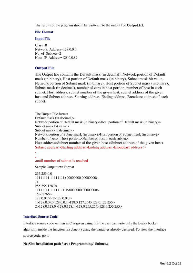
The results of the program should be written into the output file Output.txt.
File Format
Input File
Class=B
Network_Address=128.0.0.0
No_of_Subnets=2
Host_IP_Address=128.0.0.89
Output File
The Output file contains the Default mask (in decimal), Network portion of Default
mask (in binary), Host portion of Default mask (in binary), Subnet mask bit value,
Network portion of Subnet mask (in binary), Host portion of Subnet mask (in binary),
Subnet mask (in decimal), number of zero in host portion, number of host in each
subnet, Host address, subnet number of the given host, subnet address of the given
host and Subnet address, Starting address, Ending address, Broadcast address of each
subnet.
The Output File format
Default mask (in decimal)>
Network portion of Default mask (in binary)>Host portion of Default mask (in binary)>
Subnet mask bit value>
Subnet mask (in decimal)>
Network portion of Subnet mask (in binary)>Host portion of Subnet mask (in binary)>
Number of zero in host portion,>Number of host in each subnet>
Host address>Subnet number of the given host >Subnet address of the given host>
Subnet address>Starting address>Ending address>Broadcast address >
.
.
.until number of subnet is reached
Sample Output text Format
255.255.0.0
11111111 11111111>00000000 00000000>
1>
255.255.128.0>
11111111 11111111 1>0000000 00000000>
15>32766>
128.0.0.89>1>128.0.0.0>
1>128.0.0.0>128.0.0.1>128.0.127.254>128.0.127.255>
2>128.0.128.0>128.0.128.1>128.0.255.254>128.0.255.255>
Interface Source Code
Interface source code written in C is given using this the user can write only the Leaky bucket
algorithm inside the function fnSubnet () using the variables already declared. To view the interface
source code, go to
NetSim Installation path / src / Programming/ Subnet.c
Rev 6.2 Oct 12
To find NetSim’s Installation path right click NetSim icon and select
� Open file location in Windows 7
� Open file location in Windows Vista
� Properties --> find target in Windows XP.
Sample Scenarios:
Objective - To understand the concept of Subnetting through programming.
How to Proceed? - The objective can be executed in NetSim using the programming
exercise available, under programming user has to select Subnetting,
Sample Inputs - In the Input panel the following steps need to be done,
• Sample Mode should be selected.
• Select the Class Name
• Select the Network Address from the given list.
• Select the Number of Subnets from the given list.
• Select the Host IP Address.
• Then Run button need to be clicked. Refresh button can be used if new
Inputs have to be given.
Output - The following steps are under gone internally,
• Subnet mask value is obtained.
• Number of host in the each subnet is obtained
• Subnet address, Starting address, Ending address and Broadcast address are
obtained.
• Subnet address of the given Host IP address is obtained.
• Once the sample experiment is done, then Refresh button can be clicked to
create New Samples.
EUI-64 Interface Identifier
Programming Guidelines
This section guides the user to link his/her own code for EUI 64 Interface Identifier to NetSim.
Pre - Conditions
The user program should read the inputted scenario from text file named ‘Input’ with
extension txt.
The user program after executing the concept should write the required output to a file named
‘Output’ with extension txt.
Rev 6.2 Oct 12
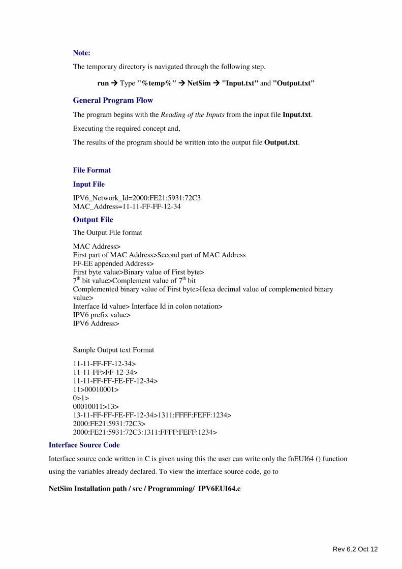
Note:
The temporary directory is navigated through the following step.
run ���� Type "%temp%" ���� NetSim ���� "Input.txt" and "Output.txt"
General Program Flow
The program begins with the Reading of the Inputs from the input file Input.txt.
Executing the required concept and,
The results of the program should be written into the output file Output.txt.
File Format
Input File
IPV6_Network_Id=2000:FE21:5931:72C3
MAC_Address=11-11-FF-FF-12-34
Output File
The Output File format
MAC Address>
First part of MAC Address>Second part of MAC Address
FF-EE appended Address>
First byte value>Binary value of First byte>
7th bit value>Complement value of 7
th bit
Complemented binary value of First byte>Hexa decimal value of complemented binary
value>
Interface Id value> Interface Id in colon notation>
IPV6 prefix value>
IPV6 Address>
Sample Output text Format
11-11-FF-FF-12-34>
11-11-FF>FF-12-34>
11-11-FF-FF-FE-FF-12-34>
11>00010001>
0>1>
00010011>13>
13-11-FF-FF-FE-FF-12-34>1311:FFFF:FEFF:1234>
2000:FE21:5931:72C3>
2000:FE21:5931:72C3:1311:FFFF:FEFF:1234>
Interface Source Code
Interface source code written in C is given using this the user can write only the fnEUI64 () function
using the variables already declared. To view the interface source code, go to
NetSim Installation path / src / Programming/ IPV6EUI64.c
Rev 6.2 Oct 12
To find NetSim’s Installation path right click NetSim icon and select
� Open file location in Windows 7
� Open file location in Windows Vista
� Properties --> find target in Windows XP.
Sample Scenarios:
Objective - To understand the concept of EUI 64 Interface Identifier through programming.
How to Proceed? - The objective can be executed in NetSim using the programming
exercise available, under programming user has to select IPV6 Addressing � EUI 64
Interface Identifier,
Sample Inputs - In the Input panel the following steps need to be done,
• Sample Mode should be selected.
• Select the IPV6 Network Id (IPV6 Prefix)
• Enter the MAC Address.
• Then Run button need to be clicked. Refresh button can be used if new
Inputs have to be given.
Output - The following steps are under gone internally,
• MAC Address is divided into two parts
• FF-FE value is appended between the two parts
• Interface Identifier is found by complementing 7th
bit of firs byte
• IPV6 Network Id (IPV6 prefix) and Interface Identifier are combined to
produce IPV6 address
• Once the sample experiment is done, then Refresh button can be clicked to
create New Samples.
IPV6 Host Addresses
Programming Guidelines
This section guides the user to link his/her own code for IPV6 Host Addresses to NetSim.
Pre - Conditions
The user program should read the inputted scenario from text file named ‘Input’ with
extension txt.
The user program after executing the concept should write the required output to a file named
‘Output’ with extension txt.
Rev 6.2 Oct 12
Note:
The temporary directory is navigated through the following step.
run ���� Type "%temp%" ���� NetSim ���� "Input.txt" and "Output.txt"
General Program Flow
The program begins with the Reading of the Inputs from the input file Input.txt.
Executing the required concept and,
The results of the program should be written into the output file Output.txt.
File Format
Input File
IPV6_Address=1111:2222:3333:4444:AAAA:BBBB:CCCC:DDDD
Prefix_Length=12
Output File
The Output File format
IPV6 Address>
Binary value of IPV6 Address>
Prefix part of IPV6 Address>Suffix part of IPV6 Address>
Prefix part of Starting Address>Suffix part of Starting Address>
Starting Address in hexa decimal notation>
Prefix part of Ending Address>Suffix part of Ending Address>
Ending Address in hexa decimal notation>
Sample Output text Format
1111:2222:3333:4444:AAAA:BBBB:CCCC:DDDD>
000100010001000100100010001000100011001100110011010001000100010010101010101
01010101110111011101111001100110011001101110111011101>
12>116>
000100010001>00010010001000100010001100110011001101000100010001001010101010
101010101110111011101111001100110011001101110111011101>
000100010001>00000000000000000000000000000000000000000000000000000000000000
000000000000000000000000000000000000000000000000000000>
1110:0000:0000:0000:0000:0000:0000:0000>
000100010001>11111111111111111111111111111111111111111111111111111111111111
111111111111111111111111111111111111111111111111111111>
111F:FFFF:FFFF:FFFF:FFFF:FFFF:FFFF:FFFF>
Interface Source Code
Interface source code written in C is given using this the user can write only the fnHostAddresses ()
function using the variables already declared. To view the interface source code, go to
NetSim Installation path / src / Programming/ IPV6HostAddress.c
To find NetSim’s Installation path right click NetSim icon and select
� Open file location in Windows 7
� Open file location in Windows Vista
Rev 6.2 Oct 12
� Properties --> find target in Windows XP.
Sample Scenarios:
Objective - To understand the concept of IPV6 Host Addresses through programming.
How to Proceed? - The objective can be executed in NetSim using the programming
exercise available, under programming user has to select IPV6 Addressing �IPV6 Host
Addresses,
Sample Inputs - In the Input panel the following steps need to be done,
• Sample Mode should be selected.
• Enter the IPV6 Address.
• Select the Prefix length.
• Then Run button need to be clicked. Refresh button can be used if new
Inputs have to be given.
Output - The following steps are under gone internally,
• IPV6 is separated into two parts: Network Id bits (prefix) and Host Id bits
(suffix)
• Starting address of the network is found by replacing each bits of suffix part
with zero
• Ending address of the network is found by replacing each bits of suffix part
with one
• Once the sample experiment is done, then Refresh button can be clicked to
create New Samples.
IPV6 Subnetting
Programming Guidelines
This section guides the user to link his/her own code for IPV6 Subnetting to NetSim.
Pre - Conditions
The user program should read the inputted scenario from text file named ‘Input’ with
extension txt.
The user program after executing the concept should write the required output to a file named
‘Output’ with extension txt.
Note:
The temporary directory is navigated through the following step.
run ���� Type "%temp%" ���� NetSim ���� "Input.txt" and "Output.txt"
Rev 6.2 Oct 12
General Program Flow
The program begins with the Reading of the Inputs from the input file Input.txt.
Executing the required concept and,
The results of the program should be written into the output file Output.txt.
File Format
Input File
IPV6_Address=1111:2222:3333:4444:AAAA:BBBB:CCCC:DDDD
Prefix_Length=12
Number_of_Subnets=2
Number_of_Level=2
Subnets_in_Level1=2
Subnets_in_Level2=4
Output File
The Output File format
Binary value of IPV6 Address>
Prefix part of IPV6 Address>Suffix part of IPV6 Address>
Number of subnets>number of subnet msk bit>
Prefix part of IPV6 Address>Subnet Id part of IPV6 address>Suffix part of IPV6
Address>
Prefix part of IPV6 Address>Subnet Id part of IPV6 address>Suffix part of IPV6
Address>
Prefix part of Level 1 ‘s first subnet Address> Subnet Id part of Level 1 ‘s first
subnet Address> Suffix part of Level 1 ‘s first subnet Address> Hexa decimal value
of Level 1 ‘s first subnet address>prefix length of Level 1 ‘s first subnet>
.
.
until number of subnet reached in the first level
First level’s subnet number>Prefix part of Level 2 ‘s first subnet Address> Subnet Id
part of Level 2 ‘s first subnet Address> Suffix part of Level 2 ‘s first subnet
Address> Hexa decimal value of Level 2 ‘s first subnet address>prefix length of
Level 2 ‘s first subnet>
.
.
until the number of subnets reached in the second level of first level’s subnet
.
.
until the number of subnets reached in the first level
Sample Output text Format
1111:2222:3333:4444:AAAA:BBBB:CCCC:DDDD>
000100010001100100100010001000100011001100110011010001000100010010101010101
01010101110111011101111001100110011001101110111011101>
000100010001>00010010001000100010001100110011001101000100010001001010101010
101010101110111011101111001100110011001101110111011101>
2>1>
Rev 6.2 Oct 12
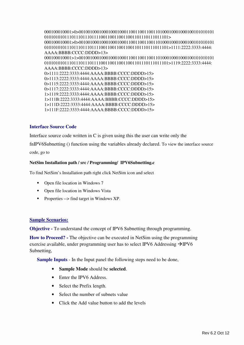
000100010001>0>001001000100010001000110011001100110100010001000100101010101
0101010101110111011101111001100110011001101110111011101>
000100010001>0>001001000100010001000110011001100110100010001000100101010101
0101010101110111011101111001100110011001101110111011101>1111:2222:3333:4444:
AAAA:BBBB:CCCC:DDDD>13>
000100010001>1>001001000100010001000110011001100110100010001000100101010101
0101010101110111011101111001100110011001101110111011101>1119:2222:3333:4444:
AAAA:BBBB:CCCC:DDDD>13>
0>1111:2222:3333:4444:AAAA:BBBB:CCCC:DDDD>15>
0>1113:2222:3333:4444:AAAA:BBBB:CCCC:DDDD>15>
0>1115:2222:3333:4444:AAAA:BBBB:CCCC:DDDD>15>
0>1117:2222:3333:4444:AAAA:BBBB:CCCC:DDDD>15>
1>1119:2222:3333:4444:AAAA:BBBB:CCCC:DDDD>15>
1>111B:2222:3333:4444:AAAA:BBBB:CCCC:DDDD>15>
1>111D:2222:3333:4444:AAAA:BBBB:CCCC:DDDD>15>
1>111F:2222:3333:4444:AAAA:BBBB:CCCC:DDDD>15>
Interface Source Code
Interface source code written in C is given using this the user can write only the
fnIPV6Subnetting () function using the variables already declared. To view the interface source
code, go to
NetSim Installation path / src / Programming/ IPV6Subnetting.c
To find NetSim’s Installation path right click NetSim icon and select
� Open file location in Windows 7
� Open file location in Windows Vista
� Properties --> find target in Windows XP.
Sample Scenarios:
Objective - To understand the concept of IPV6 Subnetting through programming.
How to Proceed? - The objective can be executed in NetSim using the programming
exercise available, under programming user has to select IPV6 Addressing �IPV6
Subnetting,
Sample Inputs - In the Input panel the following steps need to be done,
• Sample Mode should be selected.
• Enter the IPV6 Address.
• Select the Prefix length.
• Select the number of subnets value
• Click the Add value button to add the levels
Rev 6.2 Oct 12
• Then Run button need to be clicked. Refresh button can be used if new
Inputs have to be given.
Output - The following steps are under gone internally,
• IPV6 is separated into two parts: prefix and suffix
• Number of subnet mask id is calculated
• Then Subnet Id portion is derived from suffix part
• Using the subnet id portion, subnets are calculated
• Like that, subnets in the all levels are calculates by using the above steps
• Once the sample experiment is done, then Refresh button can be clicked to
create New Samples.
Leaky Bucket Algorithm
Programming Guidelines
This section guides the user to link his/her own code for Leaky Bucket Algorithm to NetSim.
Pre - Conditions
The user program should read the inputted scenario from text file named ‘Input’ with
extension txt.
The user program after executing the concept should write the required output to a file
named ‘Output’ with extension txt.
The path of the input file and the output file can be viewed on clicking the Button
“Path” in NetSim.
Note:
The temporary directory is navigated through the following step.
run ���� Type "%temp%" ���� NetSim ���� "Input.txt" and "Output.txt"
General Program Flow
The program begins with the Reading of the Inputs from the input file Input.txt.
Executing the required concept and,
The results of the program should be written into the output file Output.txt.
Rev 6.2 Oct 12
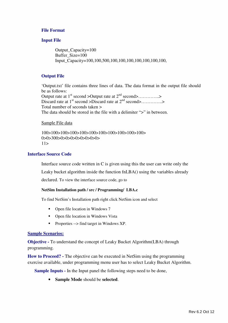
File Format
Input File
Output_Capacity=100
Buffer_Size=100
Input_Capacity=100,100,500,100,100,100,100,100,100,100,
Output File
‘Output.txt’ file contains three lines of data. The data format in the output file should
be as follows:
Output rate at 1st second >Output rate at 2
nd second>…………..>
Discard rate at 1st second >Discard rate at 2
nd second>…………..>
Total number of seconds taken >
The data should be stored in the file with a delimiter “>” in between.
Sample File data
100>100>100>100>100>100>100>100>100>100>100>
0>0>300>0>0>0>0>0>0>0>0>
11>
Interface Source Code
Interface source code written in C is given using this the user can write only the
Leaky bucket algorithm inside the function fnLBA() using the variables already
declared. To view the interface source code, go to
NetSim Installation path / src / Programming/ LBA.c
To find NetSim’s Installation path right click NetSim icon and select
� Open file location in Windows 7
� Open file location in Windows Vista
� Properties --> find target in Windows XP.
Sample Scenarios:
Objective - To understand the concept of Leaky Bucket Algorithm(LBA) through
programming.
How to Proceed? - The objective can be executed in NetSim using the programming
exercise available, under programming menu user has to select Leaky Bucket Algorithm.
Sample Inputs - In the Input panel the following steps need to be done,
• Sample Mode should be selected.
Rev 6.2 Oct 12

• Select the Output Capacity from the given list of values. The value ranges
from 100 to 1000.
• Select the Size of Buffer from the given list of values. The value ranges from
100 to 1000.
• Enter in the Input Capacity in the fields provided. The range that can be
entered is from 100 to 1000. These values will be plotted in the graph on the
right hand side panel.
• Then Run button need to be clicked. Refresh button can be used if new
Inputs have to be given.
Output - The following steps are under gone internally,
• Once the Run button is clicked a graph with Output and Discard Rate is
obtained.
• The graph explains in detail as in what is the Output and Discard Packet Rate
for the given inputs.
• Once the sample experiment is done, then Refresh button can be clicked to
create New Samples.
Multi Level Multi Access
Programming Guidelines
This section guides the user to link his/her own code for Multi-Level Multi Access Protocol
to NetSim.
Pre - Condition
User written program should read the value from the ‘Input.txt’ in the temporary
directory which is having input from the GUI at runtime
The output should be stored in ‘Output.txt’ in the temporary directory for display.
User written program should return an integer value.
Note:
The temporary directory is navigated through the following step.
run ���� Type "%temp%" ���� NetSim ���� "Input.txt" and "Output.txt"
General Program Flow
The program begins with the Reading of the Inputs from the input file Input.txt.
Executing the required concept and, The results of the program should be written into
the output file Output.txt.
Note: The naming of the input and the output file must be same as the text displayed
in the Methodology screen
Rev 6.2 Oct 12
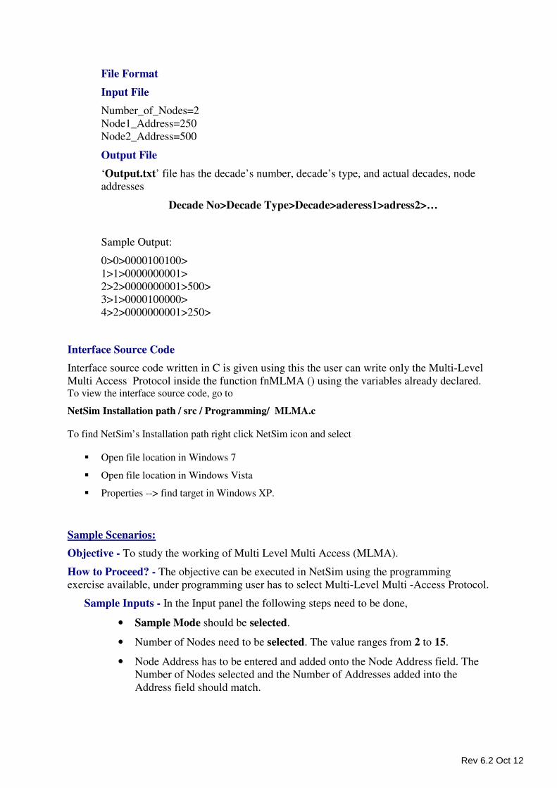
File Format
Input File
Number_of_Nodes=2
Node1_Address=250
Node2_Address=500
Output File
‘Output.txt’ file has the decade’s number, decade’s type, and actual decades, node
addresses
Decade No>Decade Type>Decade>aderess1>adress2>…
Sample Output:
0>0>0000100100>
1>1>0000000001>
2>2>0000000001>500>
3>1>0000100000>
4>2>0000000001>250>
Interface Source Code
Interface source code written in C is given using this the user can write only the Multi-Level
Multi Access Protocol inside the function fnMLMA () using the variables already declared. To view the interface source code, go to
NetSim Installation path / src / Programming/ MLMA.c
To find NetSim’s Installation path right click NetSim icon and select
� Open file location in Windows 7
� Open file location in Windows Vista
� Properties --> find target in Windows XP.
Sample Scenarios:
Objective - To study the working of Multi Level Multi Access (MLMA).
How to Proceed? - The objective can be executed in NetSim using the programming
exercise available, under programming user has to select Multi-Level Multi -Access Protocol.
Sample Inputs - In the Input panel the following steps need to be done,
• Sample Mode should be selected.
• Number of Nodes need to be selected. The value ranges from 2 to 15.
• Node Address has to be entered and added onto the Node Address field. The
Number of Nodes selected and the Number of Addresses added into the
Address field should match.
Rev 6.2 Oct 12
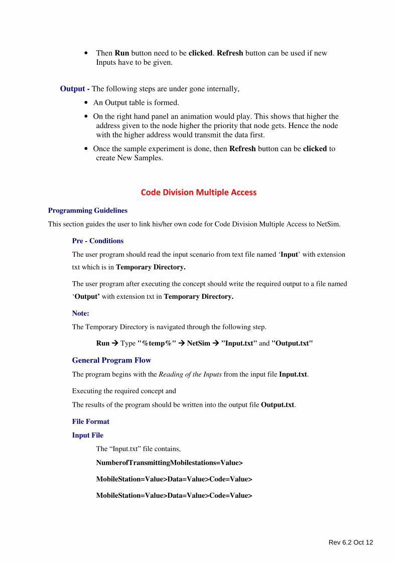
• Then Run button need to be clicked. Refresh button can be used if new
Inputs have to be given.
Output - The following steps are under gone internally,
• An Output table is formed.
• On the right hand panel an animation would play. This shows that higher the
address given to the node higher the priority that node gets. Hence the node
with the higher address would transmit the data first.
• Once the sample experiment is done, then Refresh button can be clicked to
create New Samples.
Code Division Multiple Access
Programming Guidelines
This section guides the user to link his/her own code for Code Division Multiple Access to NetSim.
Pre - Conditions
The user program should read the input scenario from text file named ‘Input’ with extension
txt which is in Temporary Directory.
The user program after executing the concept should write the required output to a file named
‘Output’ with extension txt in Temporary Directory.
Note:
The Temporary Directory is navigated through the following step.
Run ���� Type "%temp%" ���� NetSim ���� "Input.txt" and "Output.txt"
General Program Flow
The program begins with the Reading of the Inputs from the input file Input.txt.
Executing the required concept and
The results of the program should be written into the output file Output.txt.
File Format
Input File
The “Input.txt” file contains,
NumberofTransmittingMobilestations=Value>
MobileStation=Value>Data=Value>Code=Value>
MobileStation=Value>Data=Value>Code=Value>
Rev 6.2 Oct 12
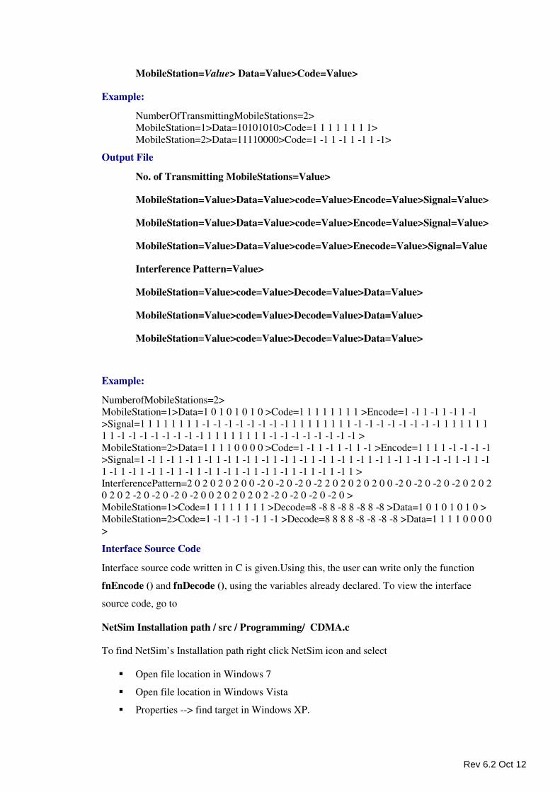
MobileStation=Value> Data=Value>Code=Value>
Example:
NumberOfTransmittingMobileStations=2>
MobileStation=1>Data=10101010>Code=1 1 1 1 1 1 1 1>
MobileStation=2>Data=11110000>Code=1 -1 1 -1 1 -1 1 -1>
Output File
No. of Transmitting MobileStations=Value>
MobileStation=Value>Data=Value>code=Value>Encode=Value>Signal=Value>
MobileStation=Value>Data=Value>code=Value>Encode=Value>Signal=Value>
MobileStation=Value>Data=Value>code=Value>Enecode=Value>Signal=Value
Interference Pattern=Value>
MobileStation=Value>code=Value>Decode=Value>Data=Value>
MobileStation=Value>code=Value>Decode=Value>Data=Value>
MobileStation=Value>code=Value>Decode=Value>Data=Value>
Example:
NumberofMobileStations=2>
MobileStation=1>Data=1 0 1 0 1 0 1 0 >Code=1 1 1 1 1 1 1 1 >Encode=1 -1 1 -1 1 -1 1 -1
>Signal=1 1 1 1 1 1 1 1 -1 -1 -1 -1 -1 -1 -1 -1 1 1 1 1 1 1 1 1 -1 -1 -1 -1 -1 -1 -1 -1 1 1 1 1 1 1
1 1 -1 -1 -1 -1 -1 -1 -1 -1 1 1 1 1 1 1 1 1 -1 -1 -1 -1 -1 -1 -1 -1 >
MobileStation=2>Data=1 1 1 1 0 0 0 0 >Code=1 -1 1 -1 1 -1 1 -1 >Encode=1 1 1 1 -1 -1 -1 -1
>Signal=1 -1 1 -1 1 -1 1 -1 1 -1 1 -1 1 -1 1 -1 1 -1 1 -1 1 -1 1 -1 1 -1 1 -1 1 -1 1 -1 -1 1 -1 1 -1
1 -1 1 -1 1 -1 1 -1 1 -1 1 -1 1 -1 1 -1 1 -1 1 -1 1 -1 1 -1 1 -1 1 >
InterferencePattern=2 0 2 0 2 0 2 0 0 -2 0 -2 0 -2 0 -2 2 0 2 0 2 0 2 0 0 -2 0 -2 0 -2 0 -2 0 2 0 2
0 2 0 2 -2 0 -2 0 -2 0 -2 0 0 2 0 2 0 2 0 2 -2 0 -2 0 -2 0 -2 0 >
MobileStation=1>Code=1 1 1 1 1 1 1 1 >Decode=8 -8 8 -8 8 -8 8 -8 >Data=1 0 1 0 1 0 1 0 >
MobileStation=2>Code=1 -1 1 -1 1 -1 1 -1 >Decode=8 8 8 8 -8 -8 -8 -8 >Data=1 1 1 1 0 0 0 0
>
Interface Source Code
Interface source code written in C is given.Using this, the user can write only the function
fnEncode () and fnDecode (), using the variables already declared. To view the interface
source code, go to
NetSim Installation path / src / Programming/ CDMA.c
To find NetSim’s Installation path right click NetSim icon and select
� Open file location in Windows 7
� Open file location in Windows Vista
� Properties --> find target in Windows XP.
Rev 6.2 Oct 12
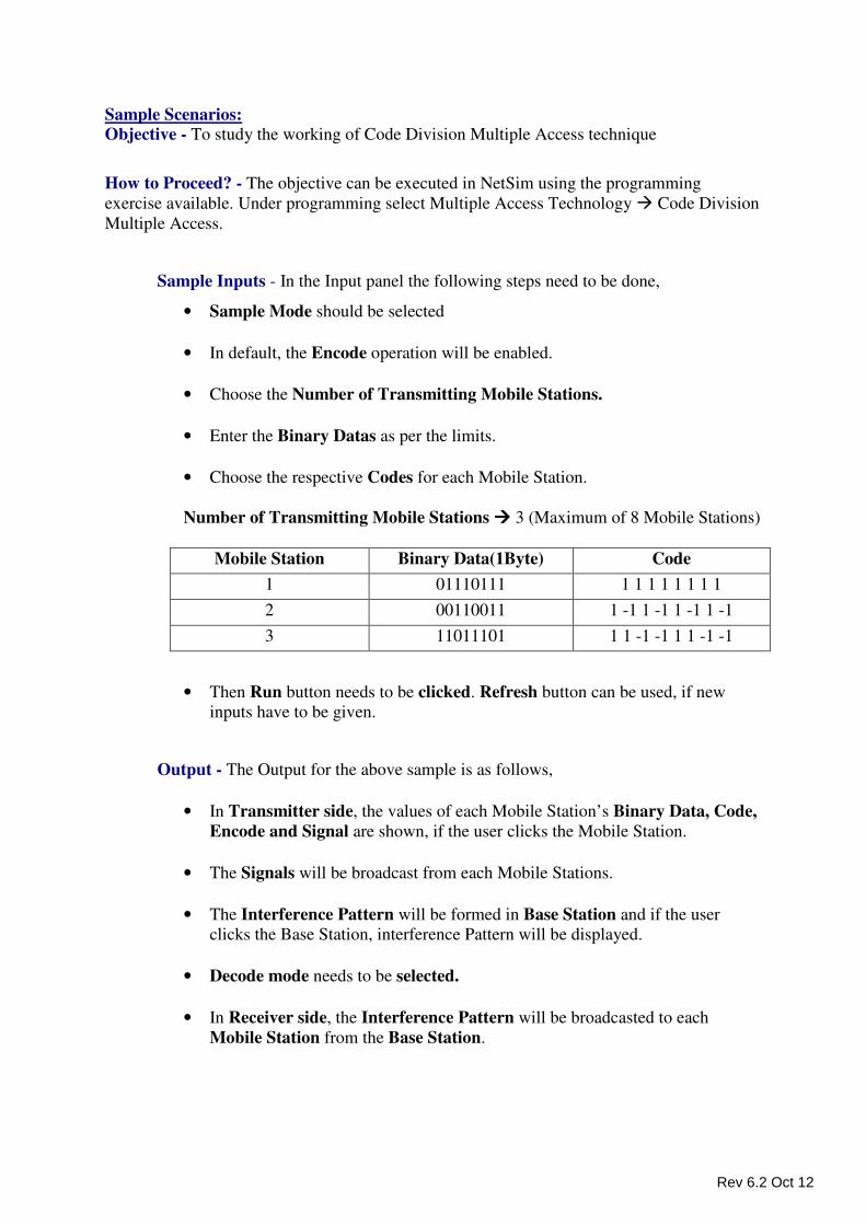
Sample Scenarios: Objective - To study the working of Code Division Multiple Access technique
How to Proceed? - The objective can be executed in NetSim using the programming
exercise available. Under programming select Multiple Access Technology � Code Division
Multiple Access.
Sample Inputs - In the Input panel the following steps need to be done,
• Sample Mode should be selected
• In default, the Encode operation will be enabled.
• Choose the Number of Transmitting Mobile Stations.
• Enter the Binary Datas as per the limits.
• Choose the respective Codes for each Mobile Station.
Number of Transmitting Mobile Stations ���� 3 (Maximum of 8 Mobile Stations)
Mobile Station Binary Data(1Byte) Code
1 01110111 1 1 1 1 1 1 1 1
2 00110011 1 -1 1 -1 1 -1 1 -1
3 11011101 1 1 -1 -1 1 1 -1 -1
• Then Run button needs to be clicked. Refresh button can be used, if new
inputs have to be given.
Output - The Output for the above sample is as follows,
• In Transmitter side, the values of each Mobile Station’s Binary Data, Code,
Encode and Signal are shown, if the user clicks the Mobile Station.
• The Signals will be broadcast from each Mobile Stations.
• The Interference Pattern will be formed in Base Station and if the user
clicks the Base Station, interference Pattern will be displayed.
• Decode mode needs to be selected.
• In Receiver side, the Interference Pattern will be broadcasted to each
Mobile Station from the Base Station.
Rev 6.2 Oct 12
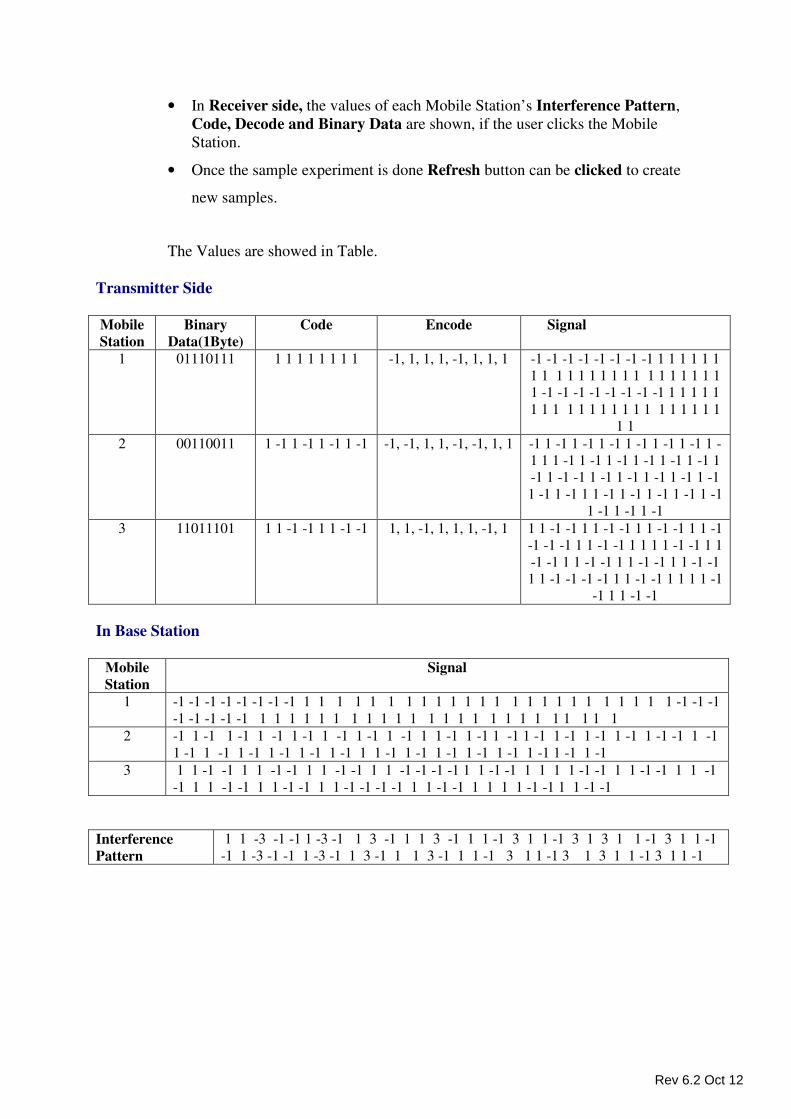
• In Receiver side, the values of each Mobile Station’s Interference Pattern,
Code, Decode and Binary Data are shown, if the user clicks the Mobile
Station.
• Once the sample experiment is done Refresh button can be clicked to create
new samples.
The Values are showed in Table.
Transmitter Side
Mobile
Station
Binary
Data(1Byte)
Code Encode Signal
1 01110111 1 1 1 1 1 1 1 1 -1, 1, 1, 1, -1, 1, 1, 1 -1 -1 -1 -1 -1 -1 -1 -1 1 1 1 1 1 1
1 1 1 1 1 1 1 1 1 1 1 1 1 1 1 1 1
1 -1 -1 -1 -1 -1 -1 -1 -1 1 1 1 1 1
1 1 1 1 1 1 1 1 1 1 1 1 1 1 1 1 1
1 1
2 00110011 1 -1 1 -1 1 -1 1 -1 -1, -1, 1, 1, -1, -1, 1, 1 -1 1 -1 1 -1 1 -1 1 -1 1 -1 1 -1 1 -
1 1 1 -1 1 -1 1 -1 1 -1 1 -1 1 -1 1
-1 1 -1 -1 1 -1 1 -1 1 -1 1 -1 1 -1
1 -1 1 -1 1 1 -1 1 -1 1 -1 1 -1 1 -1
1 -1 1 -1 1 -1
3 11011101 1 1 -1 -1 1 1 -1 -1 1, 1, -1, 1, 1, 1, -1, 1 1 1 -1 -1 1 1 -1 -1 1 1 -1 -1 1 1 -1
-1 -1 -1 1 1 -1 -1 1 1 1 1 -1 -1 1 1
-1 -1 1 1 -1 -1 1 1 -1 -1 1 1 -1 -1
1 1 -1 -1 -1 -1 1 1 -1 -1 1 1 1 1 -1
-1 1 1 -1 -1
In Base Station
Mobile
Station
Signal
1 -1 -1 -1 -1 -1 -1 -1 -1 1 1 1 1 1 1 1 1 1 1 1 1 1 1 1 1 1 1 1 1 1 1 1 1 -1 -1 -1
-1 -1 -1 -1 -1 1 1 1 1 1 1 1 1 1 1 1 1 1 1 1 1 1 1 1 1 1 1 1 1
2 -1 1 -1 1 -1 1 -1 1 -1 1 -1 1 -1 1 -1 1 1 -1 1 -1 1 -1 1 -1 1 -1 1 -1 1 -1 1 -1 -1 1 -1
1 -1 1 -1 1 -1 1 -1 1 -1 1 -1 1 1 -1 1 -1 1 -1 1 -1 1 -1 1 -1 1 -1 1 -1
3 1 1 -1 -1 1 1 -1 -1 1 1 -1 -1 1 1 -1 -1 -1 -1 1 1 -1 -1 1 1 1 1 -1 -1 1 1 -1 -1 1 1 -1
-1 1 1 -1 -1 1 1 -1 -1 1 1 -1 -1 -1 -1 1 1 -1 -1 1 1 1 1 -1 -1 1 1 -1 -1
Interference
Pattern
1 1 -3 -1 -1 1 -3 -1 1 3 -1 1 1 3 -1 1 1 -1 3 1 1 -1 3 1 3 1 1 -1 3 1 1 -1
-1 1 -3 -1 -1 1 -3 -1 1 3 -1 1 1 3 -1 1 1 -1 3 1 1 -1 3 1 3 1 1 -1 3 1 1 -1
Rev 6.2 Oct 12
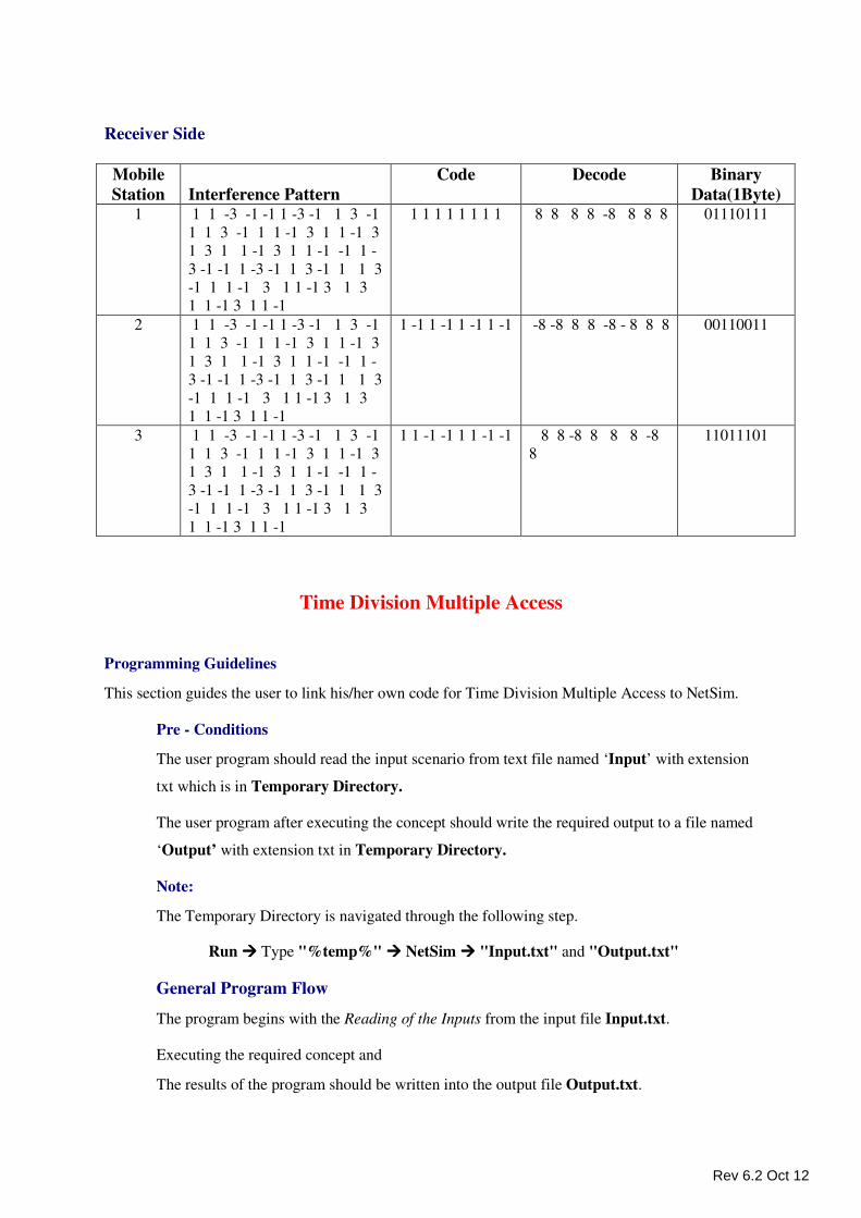
Receiver Side
Mobile
Station
Interference Pattern
Code Decode Binary
Data(1Byte) 1 1 1 -3 -1 -1 1 -3 -1 1 3 -1
1 1 3 -1 1 1 -1 3 1 1 -1 3
1 3 1 1 -1 3 1 1 -1 -1 1 -
3 -1 -1 1 -3 -1 1 3 -1 1 1 3
-1 1 1 -1 3 1 1 -1 3 1 3
1 1 -1 3 1 1 -1
1 1 1 1 1 1 1 1 8 8 8 8 -8 8 8 8 01110111
2 1 1 -3 -1 -1 1 -3 -1 1 3 -1
1 1 3 -1 1 1 -1 3 1 1 -1 3
1 3 1 1 -1 3 1 1 -1 -1 1 -
3 -1 -1 1 -3 -1 1 3 -1 1 1 3
-1 1 1 -1 3 1 1 -1 3 1 3
1 1 -1 3 1 1 -1
1 -1 1 -1 1 -1 1 -1 -8 -8 8 8 -8 - 8 8 8 00110011
3 1 1 -3 -1 -1 1 -3 -1 1 3 -1
1 1 3 -1 1 1 -1 3 1 1 -1 3
1 3 1 1 -1 3 1 1 -1 -1 1 -
3 -1 -1 1 -3 -1 1 3 -1 1 1 3
-1 1 1 -1 3 1 1 -1 3 1 3
1 1 -1 3 1 1 -1
1 1 -1 -1 1 1 -1 -1 8 8 -8 8 8 8 -8
8
11011101
Time Division Multiple Access
Programming Guidelines
This section guides the user to link his/her own code for Time Division Multiple Access to NetSim.
Pre - Conditions
The user program should read the input scenario from text file named ‘Input’ with extension
txt which is in Temporary Directory.
The user program after executing the concept should write the required output to a file named
‘Output’ with extension txt in Temporary Directory.
Note:
The Temporary Directory is navigated through the following step.
Run ���� Type "%temp%" ���� NetSim ���� "Input.txt" and "Output.txt"
General Program Flow
The program begins with the Reading of the Inputs from the input file Input.txt.
Executing the required concept and
The results of the program should be written into the output file Output.txt.
Rev 6.2 Oct 12
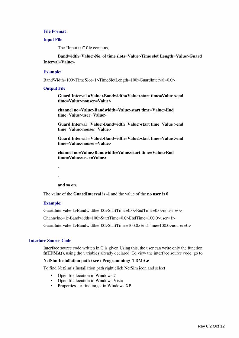
File Format
Input File
The “Input.txt” file contains,
Bandwidth=Value>No. of time slots=Value>Time slot Length=Value>Guard
Interval=Value>
Example:
BandWidth=100>TimeSlot=1>TimeSlotLength=100>GuardInterval=0.0>
Output File
Guard Interval =Value>Bandwidth=Value>start time=Value >end
time=Value>nouser=Value>
channel no=Value>Bandwidth=Value>start time=Value>End
time=Value>user=Value>
Guard Interval =Value>Bandwidth=Value>start time=Value >end time=Value>nouser=Value>
Guard Interval =Value>Bandwidth=Value>start time=Value >end time=Value>nouser=Value>
channel no=Value>Bandwidth=Value>start time=Value>End time=Value>user=Value>
.
.
and so on.
The value of the GuardInterval is -1 and the value of the no user is 0
Example:
GuardInterval=-1>Bandwidth=100>StartTime=0.0>EndTime=0.0>nouser=0>
Channelno=1>Bandwidth=100>StartTime=0.0>EndTime=100.0>user=1>
GuardInterval=-1>Bandwidth=100>StartTime=100.0>EndTime=100.0>nouser=0>
Interface Source Code
Interface source code written in C is given.Using this, the user can write only the function
fnTDMA(), using the variables already declared. To view the interface source code, go to
NetSim Installation path / src / Programming/ TDMA.c
To find NetSim’s Installation path right click NetSim icon and select
� Open file location in Windows 7
� Open file location in Windows Vista
� Properties --> find target in Windows XP.
Rev 6.2 Oct 12
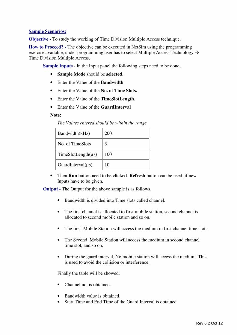
Sample Scenarios:
Objective - To study the working of Time Division Multiple Access technique.
How to Proceed? - The objective can be executed in NetSim using the programming
exercise available, under programming user has to select Multiple Access Technology �
Time Division Multiple Access.
Sample Inputs - In the Input panel the following steps need to be done,
• Sample Mode should be selected.
• Enter the Value of the Bandwidth.
• Enter the Value of the No. of Time Slots.
• Enter the Value of the TimeSlotLength.
• Enter the Value of the GuardInterval
Note:
The Values entered should be within the range.
Bandwidth(kHz) 200
No. of TimeSlots 3
TimeSlotLength(µs) 100
GuardInterval(µs) 10
• Then Run button need to be clicked. Refresh button can be used, if new
Inputs have to be given.
Output - The Output for the above sample is as follows,
• Bandwidth is divided into Time slots called channel.
• The first channel is allocated to first mobile station, second channel is
allocated to second mobile station and so on.
• The first Mobile Station will access the medium in first channel time slot.
• The Second Mobile Station will access the medium in second channel
time slot, and so on.
• During the guard interval, No mobile station will access the medium. This
is used to avoid the collision or interference.
Finally the table will be showed.
• Channel no. is obtained.
• Bandwidth value is obtained.
• Start Time and End Time of the Guard Interval is obtained
Rev 6.2 Oct 12
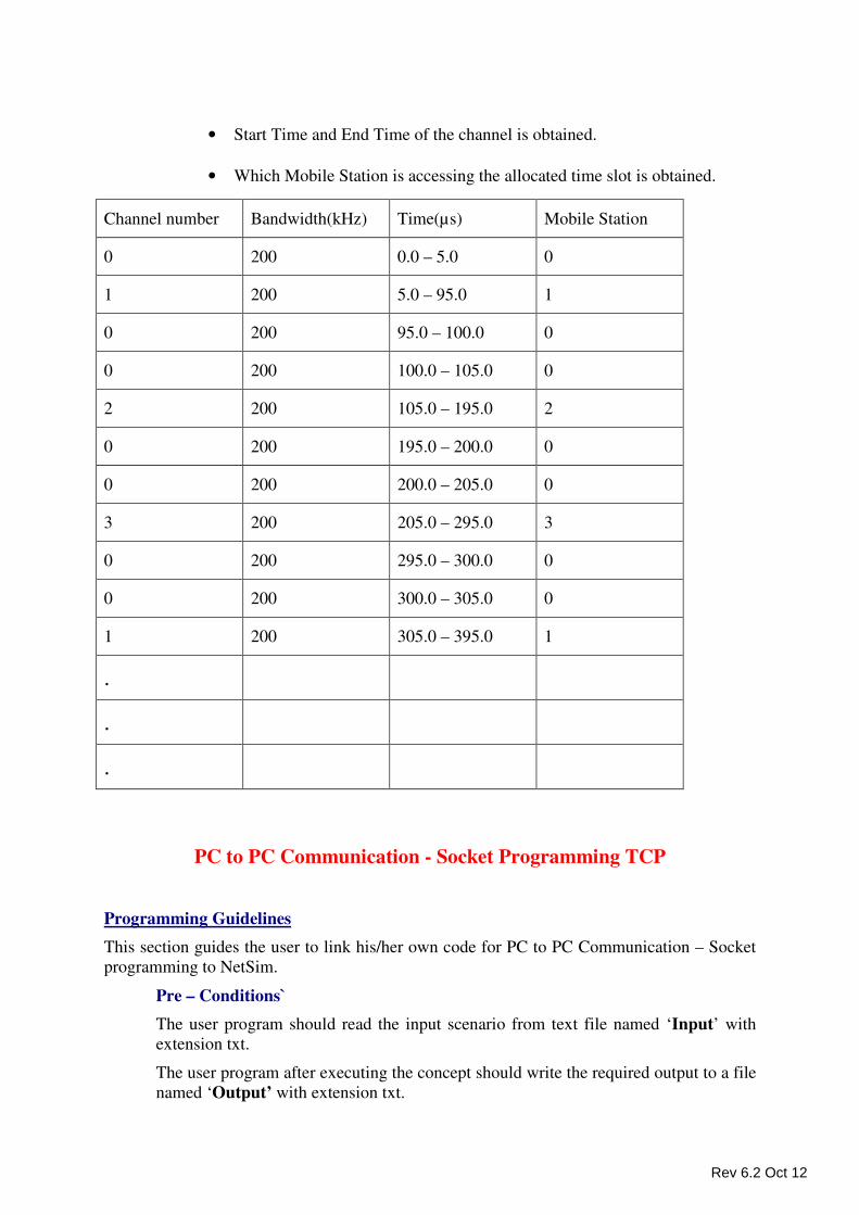
• Start Time and End Time of the channel is obtained.
• Which Mobile Station is accessing the allocated time slot is obtained.
PC to PC Communication - Socket Programming TCP
Programming Guidelines
This section guides the user to link his/her own code for PC to PC Communication – Socket
programming to NetSim.
Pre – Conditions`
The user program should read the input scenario from text file named ‘Input’ with
extension txt.
The user program after executing the concept should write the required output to a file
named ‘Output’ with extension txt.
Channel number Bandwidth(kHz) Time(µs) Mobile Station
0 200 0.0 – 5.0 0
1 200 5.0 – 95.0 1
0 200 95.0 – 100.0 0
0 200 100.0 – 105.0 0
2 200 105.0 – 195.0 2
0 200 195.0 – 200.0 0
0 200 200.0 – 205.0 0
3 200 205.0 – 295.0 3
0 200 295.0 – 300.0 0
0 200 300.0 – 305.0 0
1 200 305.0 – 395.0 1
.
.
.
Rev 6.2 Oct 12
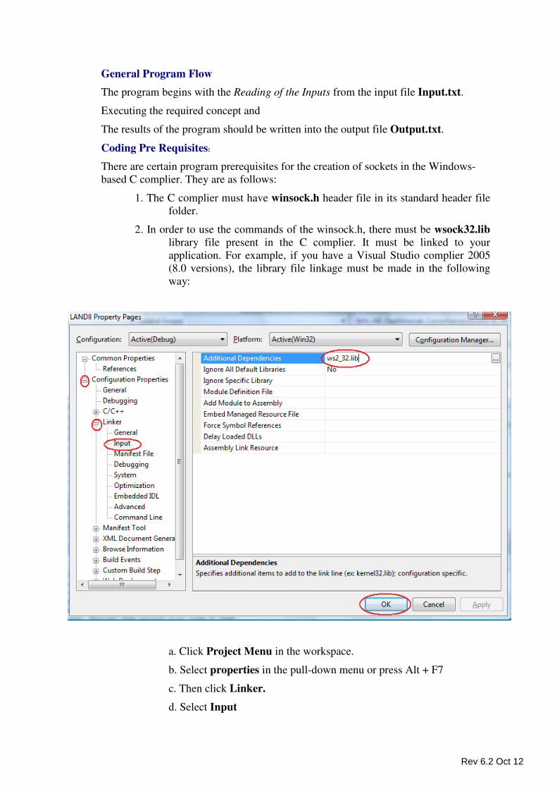
General Program Flow
The program begins with the Reading of the Inputs from the input file Input.txt.
Executing the required concept and
The results of the program should be written into the output file Output.txt.
Coding Pre Requisites:
There are certain program prerequisites for the creation of sockets in the Windows-
based C complier. They are as follows:
1. The C complier must have winsock.h header file in its standard header file
folder.
2. In order to use the commands of the winsock.h, there must be wsock32.lib
library file present in the C complier. It must be linked to your
application. For example, if you have a Visual Studio complier 2005
(8.0 versions), the library file linkage must be made in the following
way:
a. Click Project Menu in the workspace.
b. Select properties in the pull-down menu or press Alt + F7
c. Then click Linker.
d. Select Input
Rev 6.2 Oct 12
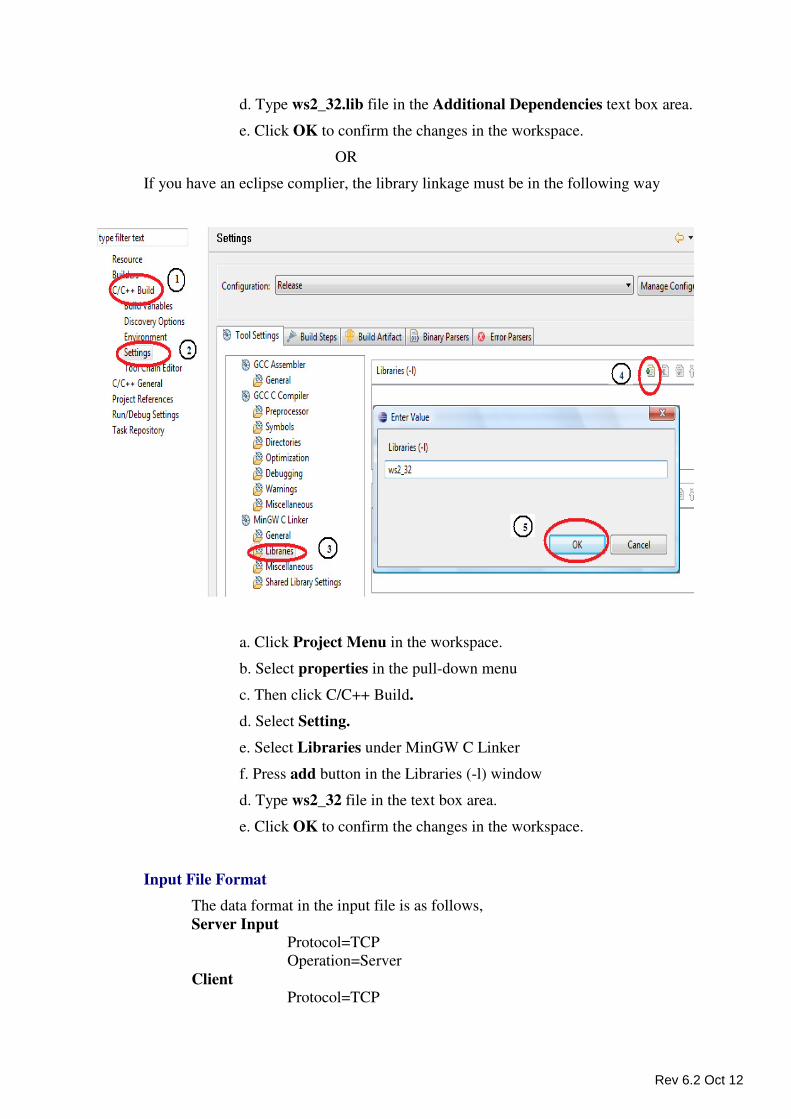
d. Type ws2_32.lib file in the Additional Dependencies text box area.
e. Click OK to confirm the changes in the workspace.
OR
If you have an eclipse complier, the library linkage must be in the following way
a. Click Project Menu in the workspace.
b. Select properties in the pull-down menu
c. Then click C/C++ Build.
d. Select Setting.
e. Select Libraries under MinGW C Linker
f. Press add button in the Libraries (-l) window
d. Type ws2_32 file in the text box area.
e. Click OK to confirm the changes in the workspace.
Input File Format
The data format in the input file is as follows,
Server Input Protocol=TCP
Operation=Server
Client Protocol=TCP
Rev 6.2 Oct 12
Operation=Client
Destination IP=192.168.0.132
<Client IP:-Message>
Ex:
192.168.0.2:- Requesting for the connection
Output File Format
Write the received message Ex:
192.168.0.2:- Requesting for the connection
Interface Source Code
Interface source code written in C is given using this the user can write only the TCP
Client () function. To view the interface source code, go to
NetSim Installation path / src / Programming/ SocketTCP.c
To find NetSim’s Installation path right click NetSim icon and select
� Open file location in Windows 7
� Open file location in Windows Vista
� Properties --> find target in Windows XP.
PC to PC Communication - Socket Programming UDP
Programming Guidelines
This section guides the user to link his/her own code for PC to PC Communication – Socket
programming to NetSim.
Pre – Conditions`
The user program should read the input scenario from text file named ‘Input’ with
extension txt.
The user program after executing the concept should write the required output to a file
named ‘Output’ with extension txt.
General Program Flow
The program begins with the Reading of the Inputs from the input file Input.txt.
Executing the required concept and
The results of the program should be written into the output file Output.txt.
Rev 6.2 Oct 12
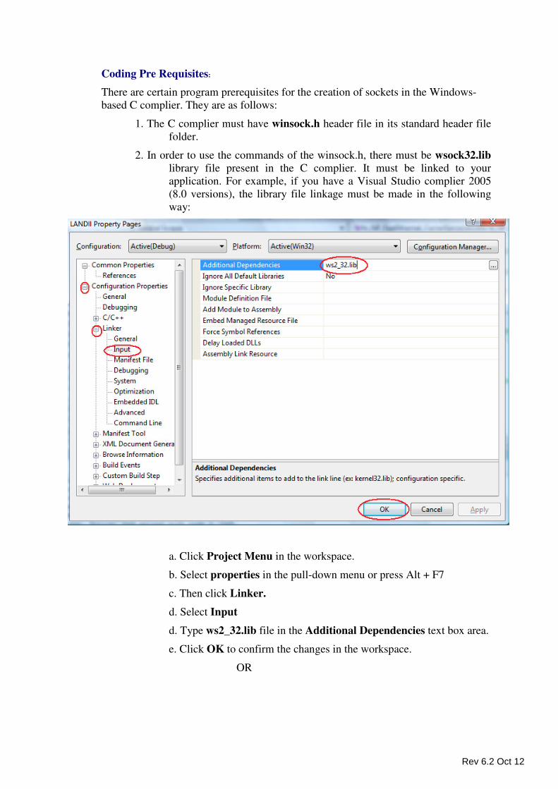
Coding Pre Requisites:
There are certain program prerequisites for the creation of sockets in the Windows-
based C complier. They are as follows:
1. The C complier must have winsock.h header file in its standard header file
folder.
2. In order to use the commands of the winsock.h, there must be wsock32.lib
library file present in the C complier. It must be linked to your
application. For example, if you have a Visual Studio complier 2005
(8.0 versions), the library file linkage must be made in the following
way:
a. Click Project Menu in the workspace.
b. Select properties in the pull-down menu or press Alt + F7
c. Then click Linker.
d. Select Input
d. Type ws2_32.lib file in the Additional Dependencies text box area.
e. Click OK to confirm the changes in the workspace.
OR
Rev 6.2 Oct 12
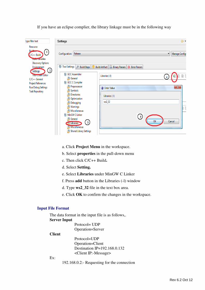
If you have an eclipse complier, the library linkage must be in the following way
a. Click Project Menu in the workspace.
b. Select properties in the pull-down menu
c. Then click C/C++ Build.
d. Select Setting.
e. Select Libraries under MinGW C Linker
f. Press add button in the Libraries (-l) window
d. Type ws2_32 file in the text box area.
e. Click OK to confirm the changes in the workspace.
Input File Format
The data format in the input file is as follows,.
Server Input Protocol= UDP
Operation=Server
Client Protocol=UDP
Operation=Client
Destination IP=192.168.0.132
<Client IP:-Message>
Ex:
192.168.0.2:- Requesting for the connection
Rev 6.2 Oct 12
Output File Format
Write the received message Ex:
192.168.0.2:- Requesting for the connection
Interface Source Code
Interface source code written in C is given using this the user can write only the UDP
() functions. To view the interface source code, go to
NetSim Installation path / src / Programming/ SocketUDP.c
To find NetSim’s Installation path right click NetSim icon and select
� Open file location in Windows 7
� Open file location in Windows Vista
� Properties --> find target in Windows XP.
Sample Scenarios:
Objective - Send and Receive the data using PC to PC Communication - Socket
Programming
How to Proceed? - Two Systems are required to perform this experiment. When one System
is in the Server Mode other should be in the Client Mode. The objective can be executed in
NetSim using the programming exercise available. In the Programming menu select PC to
PC Communication ���� Socket Programming.
Sample Inputs - By using the Input Panel that is available on the left hand side a Sample
Scenario is created. The Steps involved in creating are as follows,
• Sample Mode should be selected.
• Select a Protocol from the following,
o TCP
o UDP
• Under Operation, Server or Client should be selected.
• On the Right hand side panel there is an Input Field “Enter Data to be
Transmitted”, where Data needs to be typed in. This Data is later sent to the
Receiver System. Here Type “Hello”.
Rev 6.2 Oct 12
• Under Input there are two things,
o When Operation is Client, then the Server’s IP Address (192.168.1.2)
should be given in the Server IP Address field.
o When Operation is Server, then the Server’s IP Address (192.168.1.1)
would be automatically filled in the Local IP Address field.
Sample Output:
• On the Right hand side panel there is an Input Field “Received Data”, where
Data would get displayed. “Hello” is the Data that is received from the Client
System.
TCP
• First the Server should click on the Run button after which the Client should
click on the Run button to Create the socket
• Client should click on the Connect button to establish the connection with
server.
• The Client should click on the Send button to transmit the data to the Server.
• The Client should click on the Close button to terminate the Connection with
Server.
• If the Data is successfully transmitted then the Sent Data would be Received in
the Server System.
UDP
• First the Server should click on the Run button after which the Client should
click on the Run button to Create the socket
• The Client should click on the Send button to transmit the data to the Server.
• The Client should click on the Close button to terminate the Connection with
Server.
• If the Data is successfully transmitted then the Sent Data would be Received in
the Server System.
Rev 6.2 Oct 12
PC to PC Communication – Chat Application TCP
Programming Guidelines
This section guides the user to link his/her own code for PC to PC Communication – Socket
programming to NetSim.
Pre – Conditions
The user program should read the input scenario from text file named ‘Input’ with
extension txt.
The user program after executing the concept should write the required output to a file
named ‘Output’ with extension txt.
General Program Flow
The program begins with the Reading of the Inputs from the input file Input.txt.
Executing the required concept and
The results of the program should be written into the output file Output.txt.
Coding Pre Requisites:
There are certain program prerequisites for the creation of sockets in the Windows-
based C complier. They are as follows:
1. The C complier must have winsock.h header file in its standard header file
folder.
2. In order to use the commands of the winsock.h, there must be wsock32.lib
library file present in the C complier. It must be linked to your
application. For example, if you have a Visual Studio complier 2005
(8.0 versions), the library file linkage must be made in the following
way:
Rev 6.2 Oct 12
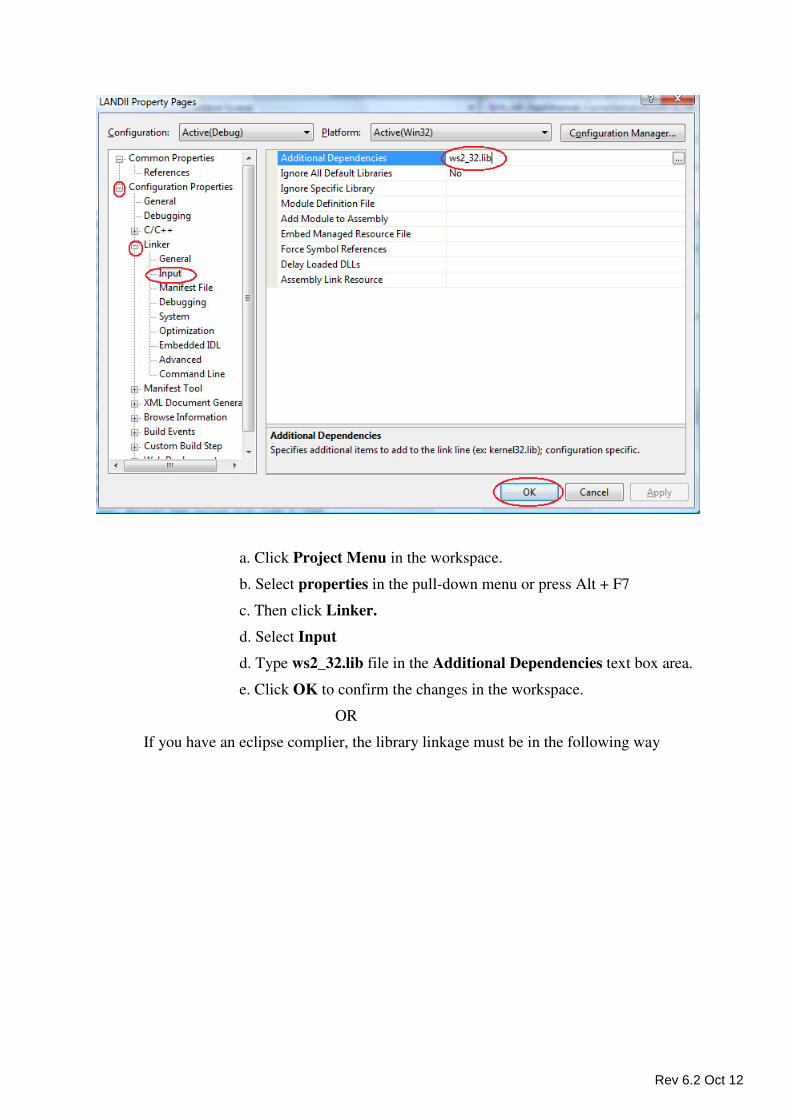
a. Click Project Menu in the workspace.
b. Select properties in the pull-down menu or press Alt + F7
c. Then click Linker.
d. Select Input
d. Type ws2_32.lib file in the Additional Dependencies text box area.
e. Click OK to confirm the changes in the workspace.
OR
If you have an eclipse complier, the library linkage must be in the following way
Rev 6.2 Oct 12
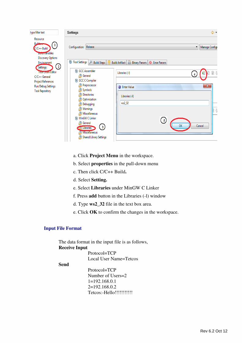
a. Click Project Menu in the workspace.
b. Select properties in the pull-down menu
c. Then click C/C++ Build.
d. Select Setting.
e. Select Libraries under MinGW C Linker
f. Press add button in the Libraries (-l) window
d. Type ws2_32 file in the text box area.
e. Click OK to confirm the changes in the workspace.
Input File Format
The data format in the input file is as follows,
Receive Input Protocol=TCP
Local User Name=Tetcos
Send Protocol=TCP
Number of Users=2
1=192.168.0.1
2=192.168.0.2
Tetcos:-Hello!!!!!!!!!!!
Rev 6.2 Oct 12
Output File Format
Write the received message Ex:
Tetcos:-Hello!!!!!!!!!!!!!!!
Interface Source Code
Interface source code written in C is given using this the user can write the TCP chat
functions. To view the interface source code, go to
NetSim Installation path / src / Programming/ ChatTCP.c
To find NetSim’s Installation path right click NetSim icon and select
� Open file location in Windows 7
� Open file location in Windows Vista
� Properties --> find target in Windows XP.
PC to PC Communication – Chat Application UDP
Programming Guidelines
This section guides the user to link his/her own code for PC to PC Communication – Socket
programming to NetSim.
Pre – Conditions`
The user program should read the input scenario from text file named ‘Input’ with
extension txt.
The user program after executing the concept should write the required output to a file
named ‘Output’ with extension txt.
General Program Flow
The program begins with the Reading of the Inputs from the input file Input.txt.
Executing the required concept and
The results of the program should be written into the output file Output.txt.
Coding Pre Requisites:
There are certain program prerequisites for the creation of sockets in the Windows-
based C complier. They are as follows:
1. The C complier must have winsock.h header file in its standard header file
folder.
Rev 6.2 Oct 12
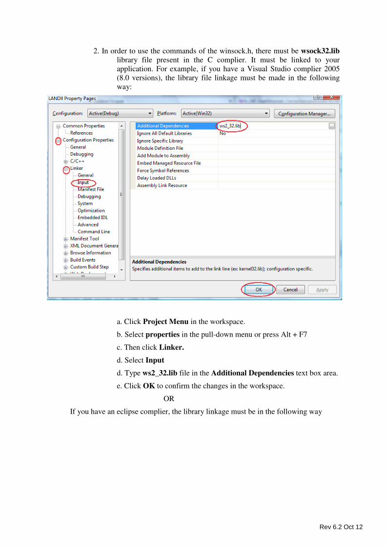
2. In order to use the commands of the winsock.h, there must be wsock32.lib
library file present in the C complier. It must be linked to your
application. For example, if you have a Visual Studio complier 2005
(8.0 versions), the library file linkage must be made in the following
way:
a. Click Project Menu in the workspace.
b. Select properties in the pull-down menu or press Alt + F7
c. Then click Linker.
d. Select Input
d. Type ws2_32.lib file in the Additional Dependencies text box area.
e. Click OK to confirm the changes in the workspace.
OR
If you have an eclipse complier, the library linkage must be in the following way
Rev 6.2 Oct 12
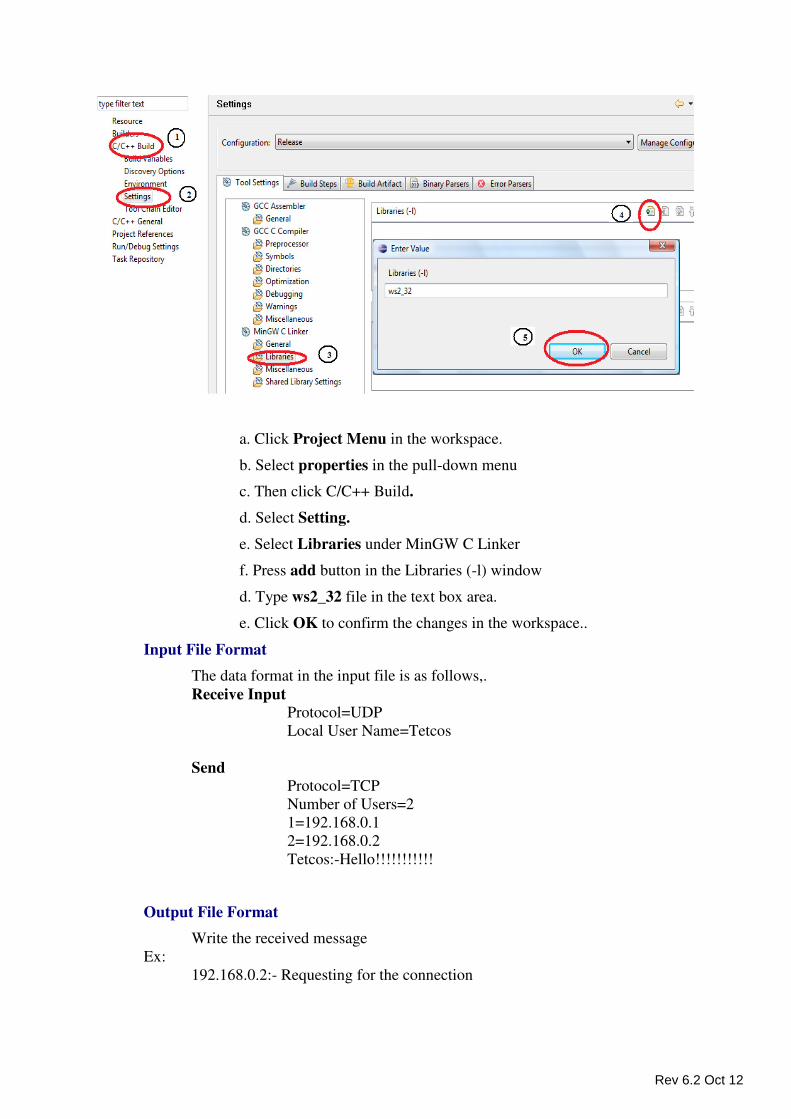
a. Click Project Menu in the workspace.
b. Select properties in the pull-down menu
c. Then click C/C++ Build.
d. Select Setting.
e. Select Libraries under MinGW C Linker
f. Press add button in the Libraries (-l) window
d. Type ws2_32 file in the text box area.
e. Click OK to confirm the changes in the workspace..
Input File Format
The data format in the input file is as follows,.
Receive Input Protocol=UDP
Local User Name=Tetcos
Send Protocol=TCP
Number of Users=2
1=192.168.0.1
2=192.168.0.2
Tetcos:-Hello!!!!!!!!!!!
Output File Format
Write the received message Ex:
192.168.0.2:- Requesting for the connection
Rev 6.2 Oct 12
Interface Source Code
Interface source code written in C is given using this the user can write UDP Chat functions.
To view the interface source code, go to
NetSim Installation path / src / Programming/ ChatUDP.c
To find NetSim’s Installation path right click NetSim icon and select
� Open file location in Windows 7
� Open file location in Windows Vista
� Properties --> find target in Windows XP.
Sample Scenarios:
Objective - Send and Receive the data using PC to PC Communication – Chat
Application
How to Proceed? - Two to Ten Systems are required to perform this experiment.
The objective can be executed in NetSim using the programming exercise available. In the
Programming menu select PC to PC Communication ���� Chat Application.
Sample Inputs - By using the Input Panel that is available on the left hand side a Sample
Scenario is created. The Steps involved in creating are as follows,
• Sample Mode should be selected.
• Select a Protocol from the following,
o TCP
o UDP
• On the Right hand side panel there is an Input Field “Send Data”, where Data
needs to be typed in. This Data is later sent to the Receiver System. Here Type
“Hello”.
• On the Right hand side panel there is “Receive Data”, where data is received
from user. Ex. “Hello”
• Under Input there are two things,
o Number of users must be select between one to ten
o Enter the IP address of the data where needs to be in all the column in the
input pane.
Rev 6.2 Oct 12
Sample Output:
• On the Right hand side panel there is an Input Field “Received Data”, where
Data would get displayed. “Hello” is the Data that is received from the users.
TCP
• Click Run button to create the socket and start Receive Data from the users.
• Click Send button to transmit the data to the users.
• Click Refresh button to terminate the connection.
UDP
• Click Run button to create the socket and start Receive Data from the users.
• Click Send button to transmit the data to the users.
Scheduling - First In First Out (FIFO)
Programming Guidelines
This section guides the user to link his/her own code for Scheduling - FIFO to NetSim.
Pre - Conditions
• The program should read the data from ‘Input.txt’ file that is available in
the temporary directory.
• The program should write the output data to ‘Output.txt’ file that is
available in the temporary directory.
Note:
The temporary directory is navigated through the following step.
run ���� Type "%temp%" ���� NetSim ���� "Input.txt" and "Output.txt"
General Program Flow
The program begins with the Reading of the Inputs from the input file Input.txt.
Executing the required concept and, the results of the program should be written into
the output file Output.txt.
Note: The naming of the input and the output file must be same as the text displayed
in the Methodology screen
File Format
Input File
Output_Link_Capacity=100
Node’s_Priority=8,7,6,5,4,3,2,1,
Rev 6.2 Oct 12
Node’s_Capacity=0,0,500,0,0,0,0,0,
Output File
Output.txt file format is as follows,
Seconds>no of bits transmitted in node 1>Transmission sequence of node 1>... no of
bits transmitted in node 8>Transmission sequence of node 8>
Sample Output File
1>0>0>0>0>100>1>0>0>0>0>0>0>0>0>0>0>
2>0>0>0>0>100>1>0>0>0>0>0>0>0>0>0>0>
3>0>0>0>0>100>1>0>0>0>0>0>0>0>0>0>0>
4>0>0>0>0>100>1>0>0>0>0>0>0>0>0>0>0>
5>0>0>0>0>100>1>0>0>0>0>0>0>0>0>0>0>
Interface Source Code
Interface source code written in C is given using this the user can write only the Scheduling
inside the function fnFIFO() using the variables already declared. To view the interface source
code, go to
NetSim Installation path / src / Programming/ FIFO.c
To find NetSim’s Installation path right click NetSim icon and select
� Open file location in Windows 7
� Open file location in Windows Vista
� Properties --> find target in Windows XP.
Sample Scenarios:
Objective - The objective is to allocate the output capacity among the various input
capacities using First In First Out (FIFO) Scheduling algorithm.
How to Proceed? - The objective can be executed in NetSim using the programming
exercise available. In the Programming menu select Scheduling.
Sample Input - By using the Input Panel that is available on the left hand side a Sample
Scenario is created. The Steps involved in creating are as follows,
• Sample Mode should be selected.
• Algorithm should be selected as First In First Out (FIFO).
• Under Input field,
0. Enter Output Link Capacity which is in MBPS. The options that are
available for selecting are 100, 200, 300, …………… 1000 MBPS. Select
400 MBPS.
Rev 6.2 Oct 12
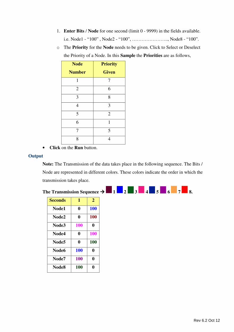
1. Enter Bits / Node for one second (limit 0 - 9999) in the fields available.
i.e. Node1 - “100” , Node2 - “100”, ………………….., Node8 - “100”.
o The Priority for the Node needs to be given. Click to Select or Deselect
the Priority of a Node. In this Sample the Priorities are as follows,
Node
Number
Priority
Given
1 7
2 6
3 8
4 3
5 2
6 1
7 5
8 4
• Click on the Run button.
Output
Note: The Transmission of the data takes place in the following sequence. The Bits /
Node are represented in different colors. These colors indicate the order in which the
transmission takes place.
The Transmission Sequence ���� 1 2 3 4 5 6 7 8.
Seconds 1 2
Node1 0 100
Node2 0 100
Node3 100 0
Node4 0 100
Node5 0 100
Node6 100 0
Node7 100 0
Node8 100 0
Rev 6.2 Oct 12
Scheduling - Max - Min Fair (MMF)
Programming Guidelines
This section guides the user to link his/her own code for Scheduling - MMF to NetSim.
Pre - Conditions
• The program should read the data from ‘Input.txt’ file that is available in
the application path.
• The program should write the output data to ‘Output.txt’ file that is
available in the application path.
Note:
The temporary directory is navigated through the following step.
run ���� Type "%temp%" ���� NetSim ���� "Input.txt" and "Output.txt"
General Program Flow
The program begins with the Reading of the Inputs from the input file Input.txt.
Executing the required concept and, the results of the program should be written into
the output file Output.txt.
Note: The naming of the input and the output file must be same as the text displayed
in the Methodology screen
File Format
Input File
Output_Link_Capacity=100
Node’s_Capacity=0,0,300,0,0,0,0,0,
Output File
‘Output.txt’ file format is as follows.
1st second >Output rate of node 1 >Priority of Node 1>………..>Output rate of node
8.Priority of Node8
2nd second >Output rate of node 1 >Priority of Node 1>………..>Output rate of node
8.Priority of Node8
Nth second >Output rate of node 1 >Priority of Node 1>………..>Output rate of node
8.Priority of Node8
Sample File data
1>0.00>0>0.00>0>100.00>1>0.00>0>0.00>0>0.00>0>0.00>0>0.00>0>
2>0.00>0>0.00>0>100.00>1>0.00>0>0.00>0>0.00>0>0.00>0>0.00>0>
3>0.00>0>0.00>0>100.00>1>0.00>0>0.00>0>0.00>0>0.00>0>0.00>0>
Rev 6.2 Oct 12
Interface Source Code
Interface source code written in C is given using this the user can write only the Scheduling
inside the function fnMMFA () using the variables already declared. To view the interface
source code, go to
NetSim Installation path / src / Programming/ MMF.c
To find NetSim’s Installation path right click NetSim icon and select
� Open file location in Windows 7
� Open file location in Windows Vista
� Properties --> find target in Windows XP.
Sample Scenarios:
Objective - The objective is to allocate the output capacity among the various input
capacities using Max-Min Fare(MMF) Scheduling algorithm.
How to Proceed? - The objective can be executed in NetSim using the programming
exercise available. In the Programming menu select Scheduling.
Sample Input - By using the Input Panel that is available on the left hand side a Sample
Scenario is created. The Steps involved in creating are as follows,
• Sample Mode should be selected.
• Algorithm should be selected as Max - Min Fair (MMF).
• Under Input field,
0. Enter Output Link Capacity which is in MBPS. The options that are
available for selecting are 100, 200, 300, …………… 1000 MBPS. Select 100
MBPS.
1. Enter Bits / Node for one second (limit 0 - 9999) in the fields available.
i.e. Node1 - “100” , Node2 - “100”, ………………….., Node8 - “100”.
• Click on the Run button.
Output
The Transmission of the data takes place in the following sequence. The Bits / Node
are represented in different colors. These colors indicate the order in which the
transmission takes place.
Rev 6.2 Oct 12
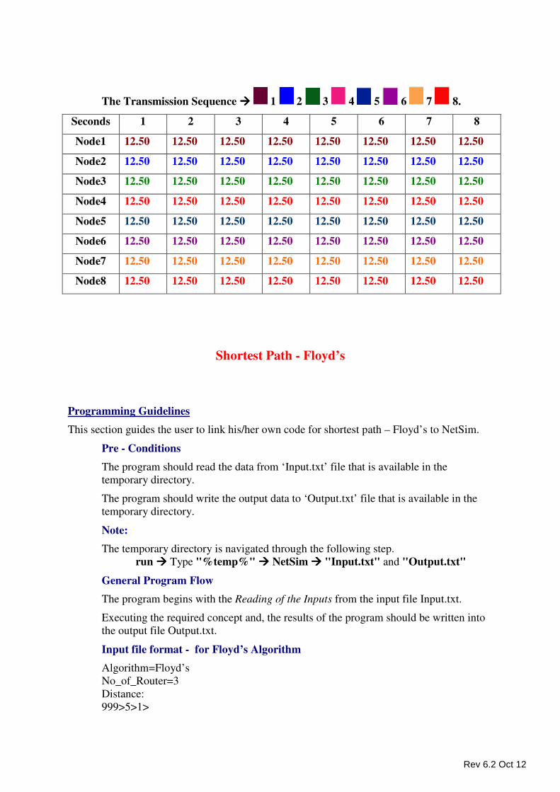
The Transmission Sequence ���� 1 2 3 4 5 6 7 8.
Seconds 1 2 3 4 5 6 7 8
Node1 12.50 12.50 12.50 12.50 12.50 12.50 12.50 12.50
Node2 12.50 12.50 12.50 12.50 12.50 12.50 12.50 12.50
Node3 12.50 12.50 12.50 12.50 12.50 12.50 12.50 12.50
Node4 12.50 12.50 12.50 12.50 12.50 12.50 12.50 12.50
Node5 12.50 12.50 12.50 12.50 12.50 12.50 12.50 12.50
Node6 12.50 12.50 12.50 12.50 12.50 12.50 12.50 12.50
Node7 12.50 12.50 12.50 12.50 12.50 12.50 12.50 12.50
Node8 12.50 12.50 12.50 12.50 12.50 12.50 12.50 12.50
Shortest Path - Floyd’s
Programming Guidelines
This section guides the user to link his/her own code for shortest path – Floyd’s to NetSim.
Pre - Conditions
The program should read the data from ‘Input.txt’ file that is available in the
temporary directory.
The program should write the output data to ‘Output.txt’ file that is available in the
temporary directory.
Note:
The temporary directory is navigated through the following step.
run ���� Type "%temp%" ���� NetSim ���� "Input.txt" and "Output.txt"
General Program Flow
The program begins with the Reading of the Inputs from the input file Input.txt.
Executing the required concept and, the results of the program should be written into
the output file Output.txt.
Input file format - for Floyd’s Algorithm
Algorithm=Floyd’s
No_of_Router=3
Distance:
999>5>1>
Rev 6.2 Oct 12
5>999>10>
1>10>999>
Source_Router=1
Destination_Router=3
Note: ‘>’ is the delimiter symbol, which is used to separate each input.
Output file format - For Floyd’s Algorithm
Consider the source node is 1
Distance>0>1>2>1>2>1>
Path>0>1>2>1>4>1>
The first line has the all the distance values from the source node to all the other
connected nodes.
The second line has the path values from the source node to all the other nodes.
The first line contains the values stored in the distance array (single dimensional
array) used in the algorithm.
The second line contains the values stored in the path array (single dimensional array)
used in the algorithm.
Sample Output:
1>2>3>
1>2>
1>3>
1>
>>>
path_FS>
0>0>0>
0>0>1>
0>1>0>
distance_FS>
0>5>1>
5>0>6>
1>6>0>
Note:
The string Distance and Path in the file is compulsory. The output must be
stored in the same format
Interface Source Code
Interface source code written in C is given using this the user can write only the Scheduling
inside the function fnFloyd() using the variables already declared. To view the interface source
code, go to
NetSim Installation path / src / Programming/ Floyds.c
Rev 6.2 Oct 12
To find NetSim’s Installation path right click NetSim icon and select
� Open file location in Windows 7
� Open file location in Windows Vista
� Properties --> find target in Windows XP.
Sample Scenarios:
Objective - The objective is to find the Shortest Path between the two Routers using the
Floyds algorithm.
How to Proceed? - The objective can be executed in NetSim using the Programming
exercise available. Under Programming Menu select Shortest Path.
Sample Input - By using the Input Panel that is available on the left hand side a Sample
Scenario is created. The Steps involved in creating are as follows,
• Sample Mode should be selected.
• Select the Algorithm as Floyd’s.
• Number of Routers needs to be selected. Minimum of 3 Routers and
Maximum of 8 Routers can be selected. Let us consider 4 Routers are selected.
• Source Router needs to be given. Let Router 4 be the Source Router.
• Destination Router also needs to be given. Let Router 1 be the Destination
Router.
• Click on 2 Routers to give the distance between those 2 Routers. A blue arrow
would be pointing from the Source Node to the Destination Node. The Distances
between the Routers that needs to be given are as follows,
0. Router 4 and Router 1 � 67 Km,
1. Router 4 and Router 3 � 46 Km,
2. Router 3 and Router 1 � 18 Km,
3. Router 3 and Router 2 � 56 Km, and
4. Router 1 and Router 2 � 70 Km.
• Click on Run button to view the output in the Routing Table.
Output - The Output for the above Scenario is as follows,
• Click the Run button to view program output.
• The Output is obtained in a Routing Table. All possible Routes and the
corresponding Distance are obtained. Below is a Routing Table for the above
Inputs,
Rev 6.2 Oct 12
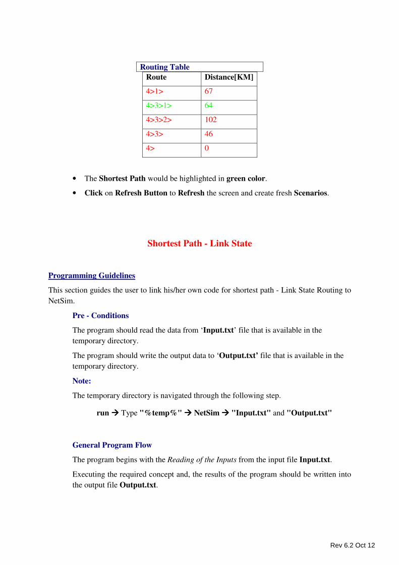
• The Shortest Path would be highlighted in green color.
• Click on Refresh Button to Refresh the screen and create fresh Scenarios.
Shortest Path - Link State
Programming Guidelines
This section guides the user to link his/her own code for shortest path - Link State Routing to
NetSim.
Pre - Conditions
The program should read the data from ‘Input.txt’ file that is available in the
temporary directory.
The program should write the output data to ‘Output.txt’ file that is available in the
temporary directory.
Note:
The temporary directory is navigated through the following step.
run ���� Type "%temp%" ���� NetSim ���� "Input.txt" and "Output.txt"
General Program Flow
The program begins with the Reading of the Inputs from the input file Input.txt.
Executing the required concept and, the results of the program should be written into
the output file Output.txt.
Routing Table
Route Distance[KM]
4>1> 67
4>3>1> 64
4>3>2> 102
4>3> 46
4> 0
Rev 6.2 Oct 12
Input file format - For Link State Algorithm
Input.txt contains the distance matrix given by the user, along with the source node,
destination node and the total number of nodes. Here, we have the input as a
SYMMETRIC matrix. The format of input.txt is, for example,
Algorithm=Link_State
No_of_Router=3
Distance:
999>6>5>
6>999>7>
5>7>999>
Source_Router=1
Destination_Router=2
Note:
‘>’ is the delimiter symbol, which is used to separate each input.
Output file format - For Link State Algorithm
Consider the source node is 1
Distance>0>1>2>1>2>1>
Path>0>1>2>1>4>1>
The first line has the all the distance values from the source node to all the other
connected nodes.
The second line has the path values from the source node to all the other nodes.
The first line contains the values stored in the distance array (single dimensional
array) used in the algorithm.
The second line contains the values stored in the path array (single dimensional array)
used in the algorithm.
Sample Output:
1>2>
1>3>2>
1>3>
1>
>>>
Distance>0>6>5>
Path>1000>1>1>
Note:
The string Distance and Path in the file is compulsory. The output must be stored in
the same format.
Rev 6.2 Oct 12
Interface Source Code
Interface source code written in C is given using this the user can write only the
Scheduling inside the function fnDijkstra() using the variables already declared. To
view the interface source code, go to
NetSim Installation path / src / Programming/ LinkState.c
To find NetSim’s Installation path right click NetSim icon and select
� Open file location in Windows 7
� Open file location in Windows Vista
� Properties --> find target in Windows XP.
Sample Scenarios:
Objective - The objective is to find the Shortest Path between the two routers using the
Link State algorithm.
How to Proceed? - Under Programming Menu select Shortest Path.
Sample Input - By using the Input Panel that is available on the left hand side a Sample Scenario is
created. The Steps involved in creating are as follows,
• Sample Mode should be selected.
• Select the Algorithm as Runed State.
• Number of Routers needs to be selected. Minimum of 3 Routers and Maximum of 8
Routers can be selected. Select 5 Routers.
• Source Router needs to be given. Let Router 5 be the Source Router.
• Destination Router also needs to be given. Let Router 3 be the Destination Router.
• Click on 2 Routers to give the distance between those 2 Routers. A blue Line would be
pointing from the Source Node to the Destination Node. The Distances between the
Routers that needs to be given are as follows,
0. Router 1 and Router 2 � 35,
1. Router 2 and Router 3 � 30,
2. Router 3 and Router 4 � 60,
3. Router 4 and Router 1 � 20,
4. Router 4 and Router 5 � 67, and
5. Router 5 and Router 2 � 58.
• Click on Run button to view the output in the Routing Table.
Rev 6.2 Oct 12
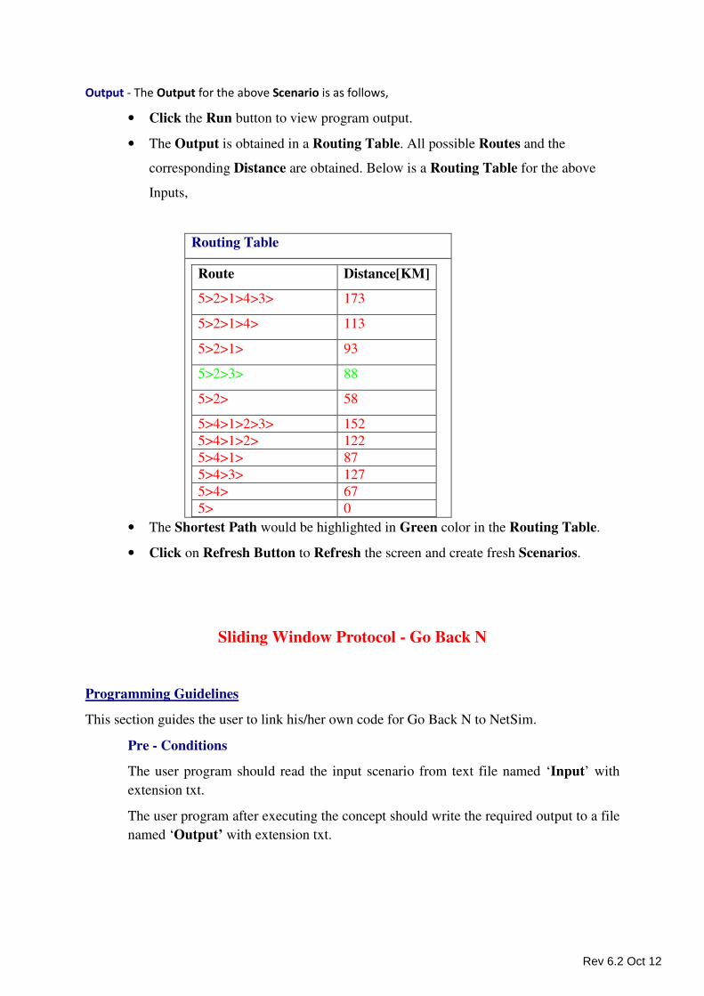
Output - The Output for the above Scenario is as follows,
• Click the Run button to view program output.
• The Output is obtained in a Routing Table. All possible Routes and the
corresponding Distance are obtained. Below is a Routing Table for the above
Inputs,
Routing Table
Route Distance[KM]
5>2>1>4>3> 173
5>2>1>4> 113
5>2>1> 93
5>2>3> 88
5>2> 58
5>4>1>2>3> 152
5>4>1>2> 122
5>4>1> 87
5>4>3> 127
5>4> 67
5> 0
• The Shortest Path would be highlighted in Green color in the Routing Table.
• Click on Refresh Button to Refresh the screen and create fresh Scenarios.
Sliding Window Protocol - Go Back N
Programming Guidelines
This section guides the user to link his/her own code for Go Back N to NetSim.
Pre - Conditions
The user program should read the input scenario from text file named ‘Input’ with
extension txt.
The user program after executing the concept should write the required output to a file
named ‘Output’ with extension txt.
Rev 6.2 Oct 12
Note:
The temporary directory is navigated through the following step.
run ���� Type "%temp%" ���� NetSim ���� "Input.txt" and "Output.txt"
General Program Flow
The program begins with the Reading of the Inputs from the input file Input.txt.
Executing the required concept and
The results of the program should be written into the output file Output.txt.
Window Size:
The Window Size for Go Back N is 7
Input File Format
Algorithm=Go_Back_N
Data_File=C:\Users\P.Sathishkumar\Documents\1 Th.txt>
Bit_Error_Rate=6
Sequence_Number=3
Window_Size=7
Output File Format
Value1>Value2>Value3>Value4>
Types: There are five types of formats of writing in the output file.
Each format is written in specific condition, the types are explained below.
The condition of writing the types is explained in the algorithm.
Type1: Value1 - "CNT",
Value 2 -output of the slidingcount function
Value 3 - "FRAMES"
Value 4 - "TRANSMIT"
Type2: Value1 - "DT",
Value 2 -Frame number,
Value 3 - Frame’s Source address,
Value 4 - Frame’s Destination address.
Type3:
Value 1 - "EV",
Value 2 - Output of the intro_error function,
Value 3 - Frame’ Source address,
Value 4 - Frame’s Destination address.
Type4:
Value 1 - "ACK",
Value 2 - "POS",
Value 3 - Acknowledgement frame’s Source Address,
Value 4 - Acknowledgement frame’s Destination Address.
Rev 6.2 Oct 12
Type5:
Value 1 - "DEL"
Value 2 - count of frames being deleted
Value 3 - "FRAME"
Value 4 - "DELETED"
Note: The above convention to write into the ‘Output.Txt’ is
mandatory.
Values in Quotes"" to be written into file ‘Output.Txt’ as it is including
Case.
DT>Frame No>node1>node2> (DT denotes Data from node 1 to node 2)
EV>Error Flag>node1>node2> (EV denotes Error Value - i.e If the above
frame has error then set the error flag as 1 else set the flag as 0)
ACK>POS>node2>node1> (Acknowledgement for that above frame received
is sent to node 2 to node 1)
Ex:
CNT>1>FRAMES>TRANSMIT>
DT>1>node1>node2>
EV>0>node1>node2>
ACK>POS>node1>node2>
Interface Source Code
Interface source code written in C is given using this the user can write only the Sliding
Window Protocols - Go Back N inside the function GoBackN () using the variables already
declared. To view the interface source code, go to
NetSim Installation path / src / Programming/ GobackN_SW.c
To find NetSim’s Installation path right click NetSim icon and select
� Open file location in Windows 7
� Open file location in Windows Vista
� Properties --> find target in Windows XP.
Sample Scenarios:
Objective - Send and receive the data using Sliding Window Protocol - Go Back N.
How to Proceed? - The objective can be executed in NetSim using the programming
exercise available. Under Programming Menu select Sliding Window Protocol � Go
Back N.
Sample Input - By using the Input Panel that is available on the left hand side a Sample
Scenario is created. The Steps involved in creating are as follows,
Rev 6.2 Oct 12
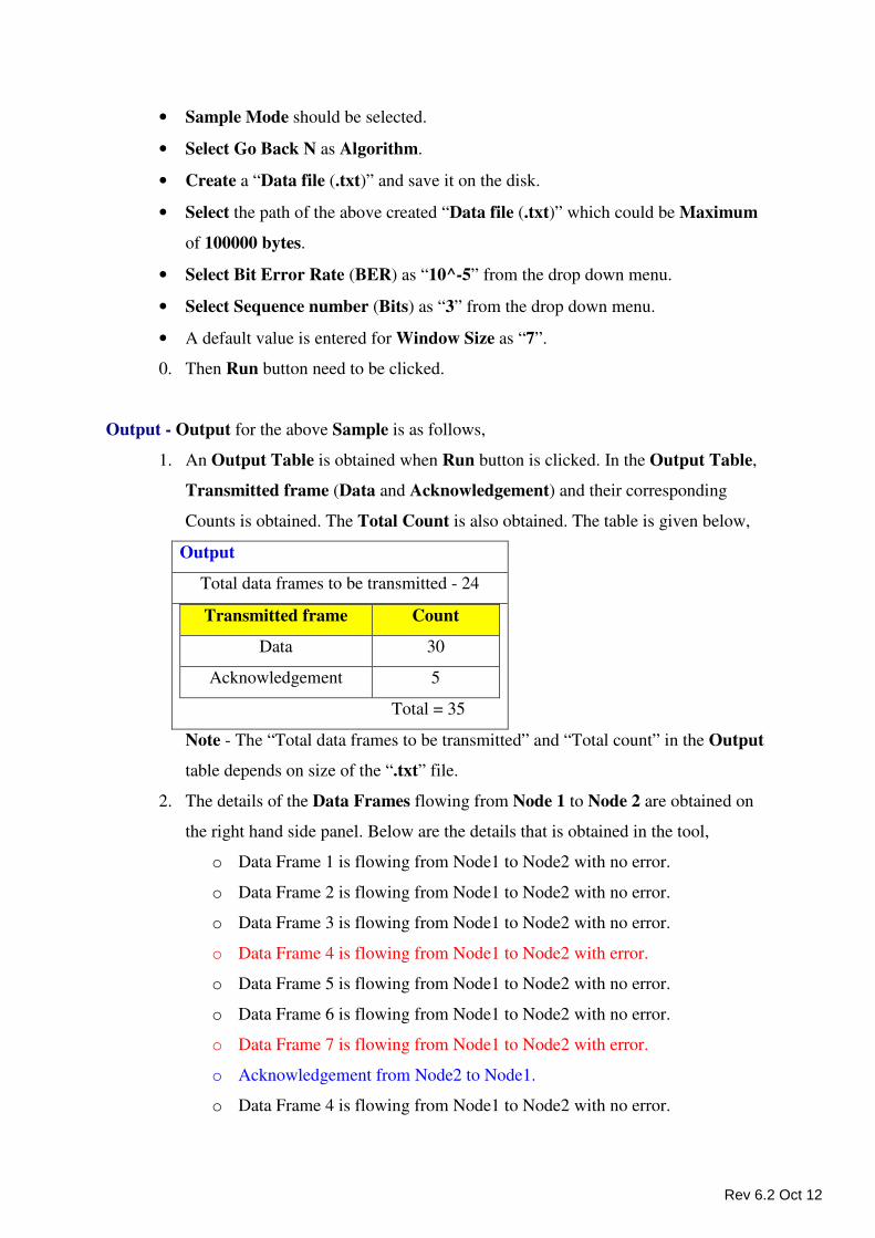
• Sample Mode should be selected.
• Select Go Back N as Algorithm.
• Create a “Data file (.txt)” and save it on the disk.
• Select the path of the above created “Data file (.txt)” which could be Maximum
of 100000 bytes.
• Select Bit Error Rate (BER) as “10^-5” from the drop down menu.
• Select Sequence number (Bits) as “3” from the drop down menu.
• A default value is entered for Window Size as “7”.
0. Then Run button need to be clicked.
Output - Output for the above Sample is as follows,
1. An Output Table is obtained when Run button is clicked. In the Output Table,
Transmitted frame (Data and Acknowledgement) and their corresponding
Counts is obtained. The Total Count is also obtained. The table is given below,
Output
Total data frames to be transmitted - 24
Transmitted frame Count
Data 30
Acknowledgement 5
Total = 35
Note - The “Total data frames to be transmitted” and “Total count” in the Output
table depends on size of the “.txt” file.
2. The details of the Data Frames flowing from Node 1 to Node 2 are obtained on
the right hand side panel. Below are the details that is obtained in the tool,
o Data Frame 1 is flowing from Node1 to Node2 with no error.
o Data Frame 2 is flowing from Node1 to Node2 with no error.
o Data Frame 3 is flowing from Node1 to Node2 with no error.
o Data Frame 4 is flowing from Node1 to Node2 with error.
o Data Frame 5 is flowing from Node1 to Node2 with no error.
o Data Frame 6 is flowing from Node1 to Node2 with no error.
o Data Frame 7 is flowing from Node1 to Node2 with error.
o Acknowledgement from Node2 to Node1.
o Data Frame 4 is flowing from Node1 to Node2 with no error.
Rev 6.2 Oct 12
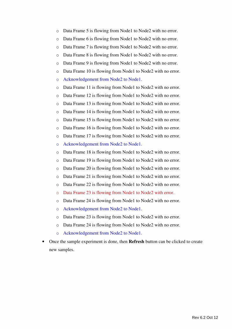
o Data Frame 5 is flowing from Node1 to Node2 with no error.
o Data Frame 6 is flowing from Node1 to Node2 with no error.
o Data Frame 7 is flowing from Node1 to Node2 with no error.
o Data Frame 8 is flowing from Node1 to Node2 with no error.
o Data Frame 9 is flowing from Node1 to Node2 with no error.
o Data Frame 10 is flowing from Node1 to Node2 with no error.
o Acknowledgement from Node2 to Node1.
o Data Frame 11 is flowing from Node1 to Node2 with no error.
o Data Frame 12 is flowing from Node1 to Node2 with no error.
o Data Frame 13 is flowing from Node1 to Node2 with no error.
o Data Frame 14 is flowing from Node1 to Node2 with no error.
o Data Frame 15 is flowing from Node1 to Node2 with no error.
o Data Frame 16 is flowing from Node1 to Node2 with no error.
o Data Frame 17 is flowing from Node1 to Node2 with no error.
o Acknowledgement from Node2 to Node1.
o Data Frame 18 is flowing from Node1 to Node2 with no error.
o Data Frame 19 is flowing from Node1 to Node2 with no error.
o Data Frame 20 is flowing from Node1 to Node2 with no error.
o Data Frame 21 is flowing from Node1 to Node2 with no error.
o Data Frame 22 is flowing from Node1 to Node2 with no error.
o Data Frame 23 is flowing from Node1 to Node2 with error.
o Data Frame 24 is flowing from Node1 to Node2 with no error.
o Acknowledgement from Node2 to Node1.
o Data Frame 23 is flowing from Node1 to Node2 with no error.
o Data Frame 24 is flowing from Node1 to Node2 with no error.
o Acknowledgement from Node2 to Node1.
• Once the sample experiment is done, then Refresh button can be clicked to create
new samples.
Rev 6.2 Oct 12
Sliding Window Protocol - Selective Repeat
Programming Guidelines
This section guides the user to link his/her own code for Selective Repeat to NetSim.
Pre - Conditions
The user program should read the input scenario from text file named ‘Input’ with
extension txt.
The user program after executing the concept should write the required output to a file
named ‘Output’ with extension txt.
Note:
The temporary directory is navigated through the following step.
run ���� Type "%temp%" ���� NetSim ���� "Input.txt" and "Output.txt"
General Program Flow
The program begins with the Reading of the Inputs from the input file Input.txt.
Executing the required concept and
The results of the program should be written into the output file Output.txt.
Window Size:
The Window Size for Selective Repeat is 7
Input File Format
Algorithm=Selective_Repeat
Data_File=C:\Users\P.Sathishkumar\Documents\1 Th.txt>
Bit_Error_Rate=5
Sequence_Number=3
Window_Size=4
Output File Format
Value1>Value2>Value3>Value4>
Types: There are five types of formats of writing in the output file.
Each format is written in specific condition, the types are explained below.
The condition of writing the types is explained in the algorithm.
Type1: Value1 - "CNT",
Value 2 - output of the slidingcount function
Value 3 - "FRAMES"
Value 4 - "TRANSMIT"
Type2: Value1 - "DT",
Rev 6.2 Oct 12
Value 2 - Frame number,
Value 3 - Frame’s Source address,
Value 4 - Frame’s Destination address.
Type3:
Value 1 - "EV",
Value 2 - Output of the intro_error function,
Value 3 - Frame’ Source address,
Value 4 - Frame’s Destination address.
Type4:
Value 1 - "ACK",
Value 2 - "POS",
Value 3 - Acknowledgement frame’s Source Address,
Value 4 - Acknowledgement frame’s Destination Address.
Type5:
Value 1 - "DEL"
Value 2 - count of frames being deleted
Value 3 - "FRAME"
Value 4 - "DELETED"
Note: The above convention to write into the ‘Output.Txt’ is
mandatory.
Values in Quotes"" to be written into file ‘Output.Txt’ as it is including
Case.
DT>Frame No>node1>node2> (DT denotes Data from node 1 to node 2)
EV>Error Flag>node1>node2> (EV denotes Error Value - i.e If the above
frame has error then set the error flag as 1 else set the flag as 0)
ACK>POS>node2>node1> (Acknowledgement for that above frame received
is sent to node 2 to node 1)
Ex: CNT>1>FRAMES>TRANSMIT>
DT>1>node1>node2>
EV>0>node1>node2>
ACK>POS>node1>node2>
Interface Source Code
Interface source code written in C is given using this the user can write only the Sliding
Window Protocol - Selective Repeat inside the function SelectiveRepeat () using the
variables already declared. To view the interface source code, go to
NetSim Installation path / src / Programming/ SelectiveRepeat_SW.c
To find NetSim’s Installation path right click NetSim icon and select
� Open file location in Windows 7
� Open file location in Windows Vista
� Properties --> find target in Windows XP.
Rev 6.2 Oct 12
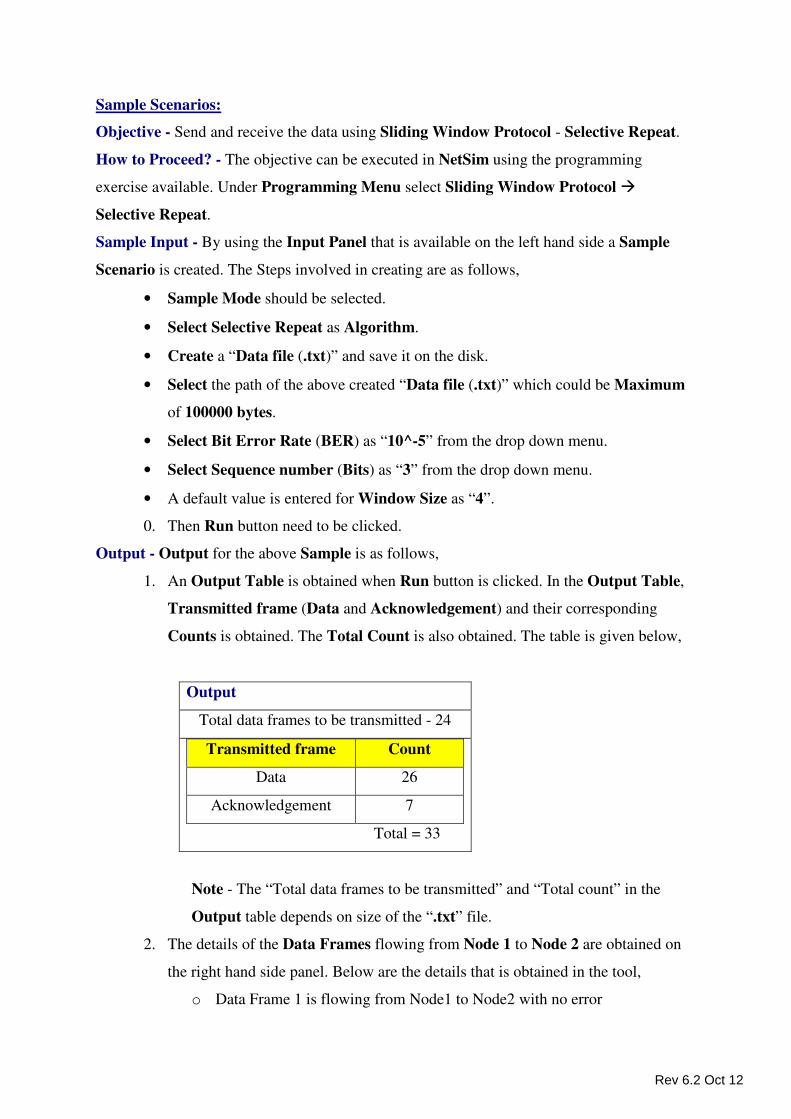
Sample Scenarios:
Objective - Send and receive the data using Sliding Window Protocol - Selective Repeat.
How to Proceed? - The objective can be executed in NetSim using the programming
exercise available. Under Programming Menu select Sliding Window Protocol �
Selective Repeat.
Sample Input - By using the Input Panel that is available on the left hand side a Sample
Scenario is created. The Steps involved in creating are as follows,
• Sample Mode should be selected.
• Select Selective Repeat as Algorithm.
• Create a “Data file (.txt)” and save it on the disk.
• Select the path of the above created “Data file (.txt)” which could be Maximum
of 100000 bytes.
• Select Bit Error Rate (BER) as “10^-5” from the drop down menu.
• Select Sequence number (Bits) as “3” from the drop down menu.
• A default value is entered for Window Size as “4”.
0. Then Run button need to be clicked.
Output - Output for the above Sample is as follows,
1. An Output Table is obtained when Run button is clicked. In the Output Table,
Transmitted frame (Data and Acknowledgement) and their corresponding
Counts is obtained. The Total Count is also obtained. The table is given below,
Output
Total data frames to be transmitted - 24
Transmitted frame Count
Data 26
Acknowledgement 7
Total = 33
Note - The “Total data frames to be transmitted” and “Total count” in the
Output table depends on size of the “.txt” file.
2. The details of the Data Frames flowing from Node 1 to Node 2 are obtained on
the right hand side panel. Below are the details that is obtained in the tool,
o Data Frame 1 is flowing from Node1 to Node2 with no error
Rev 6.2 Oct 12
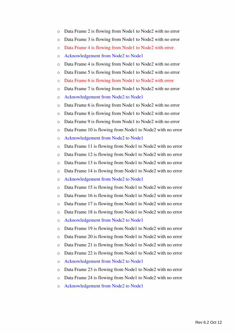
o Data Frame 2 is flowing from Node1 to Node2 with no error
o Data Frame 3 is flowing from Node1 to Node2 with no error
o Data Frame 4 is flowing from Node1 to Node2 with error
o Acknowledgement from Node2 to Node1
o Data Frame 4 is flowing from Node1 to Node2 with no error
o Data Frame 5 is flowing from Node1 to Node2 with no error
o Data Frame 6 is flowing from Node1 to Node2 with error
o Data Frame 7 is flowing from Node1 to Node2 with no error
o Acknowledgement from Node2 to Node1
o Data Frame 6 is flowing from Node1 to Node2 with no error
o Data Frame 8 is flowing from Node1 to Node2 with no error
o Data Frame 9 is flowing from Node1 to Node2 with no error
o Data Frame 10 is flowing from Node1 to Node2 with no error
o Acknowledgement from Node2 to Node1
o Data Frame 11 is flowing from Node1 to Node2 with no error
o Data Frame 12 is flowing from Node1 to Node2 with no error
o Data Frame 13 is flowing from Node1 to Node2 with no error
o Data Frame 14 is flowing from Node1 to Node2 with no error
o Acknowledgement from Node2 to Node1
o Data Frame 15 is flowing from Node1 to Node2 with no error
o Data Frame 16 is flowing from Node1 to Node2 with no error
o Data Frame 17 is flowing from Node1 to Node2 with no error
o Data Frame 18 is flowing from Node1 to Node2 with no error
o Acknowledgement from Node2 to Node1
o Data Frame 19 is flowing from Node1 to Node2 with no error
o Data Frame 20 is flowing from Node1 to Node2 with no error
o Data Frame 21 is flowing from Node1 to Node2 with no error
o Data Frame 22 is flowing from Node1 to Node2 with no error
o Acknowledgement from Node2 to Node1
o Data Frame 23 is flowing from Node1 to Node2 with no error
o Data Frame 24 is flowing from Node1 to Node2 with no error
o Acknowledgement from Node2 to Node1
Rev 6.2 Oct 12
• Once the sample experiment is done, then Refresh button can be clicked to create
new samples.
Sorting Technique - Bubble Sort
Programming Guidelines
This section guides the user to link his/her own code for Sorting Algorithm to NetSim.
Pre - Condition
User written program should read the value from the ‘Input.txt’ in the temporary
directory which is having input from the GUI at runtime
The output should be stored in ‘Output.txt’ in the temporary directory for display.
User written program should return an integer value.
Note:
The temporary directory is navigated through the following step.
run ���� Type "%temp%" ���� NetSim ���� "Input.txt" and "Output.txt"
General Program Flow
The program begins with the Reading of the Inputs from the input file Input.txt.
Executing the required concept and, The results of the program should be written into
the output file Output.txt.
Note: The naming of the input and the output file must be same as the text displayed
in the Methodology screen
File Format
Input File
Ascending Order
Sorting_Type=Bubble
Sorting_Order=Ascending
Total_Number=3
Number_to_Sort=5,4,3
Descending Order
Sorting_Type=Bubble
Sorting_Order=Descending
Total_Number=3
Number_to_Sort=4,5,6
Rev 6.2 Oct 12
Output File
type>index 1>index 2> type 0 : specifies Positioning the data value index that ha
type 1 : specifies the two index following it are being compared
type 2 : specifies the two index following it are being swapped
The following types are used in Quick Sort :
type 3 : specifies the two index, where index 1 value is copied
to index 2 value.
type 4 : specifies the two index, where Position data index
value of index1 is copied to the index 2 value.
index 1 : index 1 is the index of array that points to the first
data that is being swapped or compared.
index 2 : index 2 is the index of array that points to the second
data that is being swapped or compared.
Sample Output:
Ascending Order: 1>0>1>
2>0>1>
1>1>2>
2>1>2>
1>0>1>
2>0>1>
Descending Order: 1>0>1>
2>0>1>
1>1>2>
2>1>2>
1>0>1>
2>0>1>
Interface Source Code
Interface source code written in C is given using this the user can write only the Sorting Algorithm
inside the function fnBubblesort () using the variables already declared. To view the interface source
code, go to
NetSim Installation path / src / Programming/ BubbleSort.c
To find NetSim’s Installation path right click NetSim icon and select
� Open file location in Windows 7
� Open file location in Windows Vista
� Properties --> find target in Windows XP.
Rev 6.2 Oct 12
Sample Scenarios:
Objective - To study the working of Sorting Techniques.
How to Proceed? -
The objective can be executed in NetSim using the programming exercise available, under
programming user has to select Sorting Techniques.
Sample Inputs - In the Input panel the following steps need to be done,
• Sample Mode should be selected.
• Select the Bubble Sort as Sorting Type.
• Select the Sorting Order as either Ascending or Descending.
• Select the total number that has to be sorted. The values available are from 3
to 25.
• Enter the Number Value in the field provided. The value entered should be
within the range of 1 to 9999.
• Then Run button need to be clicked. Refresh button can be used if new
Inputs have to be given.
Output - The following steps are under gone internally,
• According to the Sorting Type selected the Output would vary.
• Number of Comparison would be obtained.
• Number of Swapping would be obtained.
• A table with the values tabulated would be obtained.
• Once the sample experiment is done, then Refresh button can be clicked to
create New Samples.
Sorting Technique - Insertion Sort
Programming Guidelines
This section guides the user to link his/her own code for Sorting Algorithm to NetSim.
Pre - Condition
User written program should read the value from the ‘Input.txt’ in the temporary
directory which is having input from the GUI at runtime
The output should be stored in ‘Output.txt’ in the temporary directory for display.
User written program should return an integer value.
Note:
The temporary directory is navigated through the following step.
run ���� Type "%temp%" ���� NetSim ���� "Input.txt" and "Output.txt"
Rev 6.2 Oct 12
General Program Flow
The program begins with the Reading of the Inputs from the input file Input.txt.
Executing the required concept and, The results of the program should be written into
the output file Output.txt.
Note: The naming of the input and the output file must be same as the text displayed
in the Methodology screen
File Format
Input File
Ascending Order
Sorting_Type=Insertion
Sorting_Order=Ascending
Total_Number=3
Number_to_Sort=9,8,7
Descending Order
Sorting_Type=Insertion
Sorting_Order=Descending
Total_Number=3
Number_to_Sort=1,9,3
Output File
type>index 1>index 2> type 0 : specifies Positioning the data value index that ha
type 1 : specifies the two index following it are being compared
type 2 : specifies the two index following it are being swapped
The following types are used in Quick Sort :
type 3 : specifies the two index, where index 1 value is copied
to index 2 value.
type 4 : specifies the two index, where Position data index
value of index1 is copied to the index 2 value.
index 1 : index 1 is the index of array that points to the first
data that is being swapped or compared.
index 2 : index 2 is the index of array that points to the second
data that is being swapped or compared.
Sample Output:
Ascending Order: 1>0>1>
2>0>1>
1>1>2>
2>1>2>
1>0>1>
2>0>1>
Rev 6.2 Oct 12
Descending Order: 1>0>1>
2>0>1>
1>1>2>
2>1>2>
1>0>1>
Interface Source Code
Interface source code written in C is given using this the user can write only the Sorting Algorithm
inside the function fnInsertsort () using the variables already declared. To view the interface source
code, go to
NetSim Installation path / src / Programming/ InsertionSort.c
To find NetSim’s Installation path right click NetSim icon and select
� Open file location in Windows 7
� Open file location in Windows Vista
� Properties --> find target in Windows XP.
Sample Project:
Objective - To study the working of Sorting Techniques.
How to Proceed? -
The objective can be executed in NetSim using the programming exercise available, under
programming user has to select Sorting Techniques.
Sample Inputs - In the Input panel the following steps need to be done,
• Sample Mode should be selected.
• Select the Insertion Sort as Sorting Type.
• Select the Sorting Order as either Ascending or Descending.
• Select the total number that has to be sorted. The values available are from 3
to 25.
• Enter the Number Value in the field provided. The value entered should be
within the range of 1 to 9999.
• Then Run button need to be clicked. Refresh button can be used if new
Inputs have to be given.
Output - The following steps are under gone internally,
• According to the Sorting Type selected the Output would vary.
• Number of Comparison would be obtained.
• Number of Swapping would be obtained.
Rev 6.2 Oct 12
• A table with the values tabulated would be obtained.
• Once the sample experiment is done, then Refresh button can be clicked to
create New Samples.
Sorting Technique - Quick Sort
Programming Guidelines
This section guides the user to link his/her own code for Sorting Algorithm to NetSim.
Pre - Condition
User written program should read the value from the ‘Input.txt’ in the temporary directory
which is having input from the GUI at runtime
The output should be stored in ‘Output.txt’ in the temporary directory for display.
User written program should return an integer value.
Note:
The temporary directory is navigated through the following step.
run ���� Type "%temp%" ���� NetSim ���� "Input.txt" and "Output.txt"
General Program Flow
The program begins with the Reading of the Inputs from the input file Input.txt.
Executing the required concept and, The results of the program should be written into the
output file Output.txt.
Note: The naming of the input and the output file must be same as the text displayed
in the Methodology screen
File Format
Input File
Ascending Order
Sorting_Type=Quick
Sorting_Order=Ascending
Total_Number=3
Number_to_Sort=33,22,66
Descending Order
Sorting_Type=Quick
Sorting_Order=Descending
Total_Number=3
Number_to_Sort=22,33,44
Rev 6.2 Oct 12
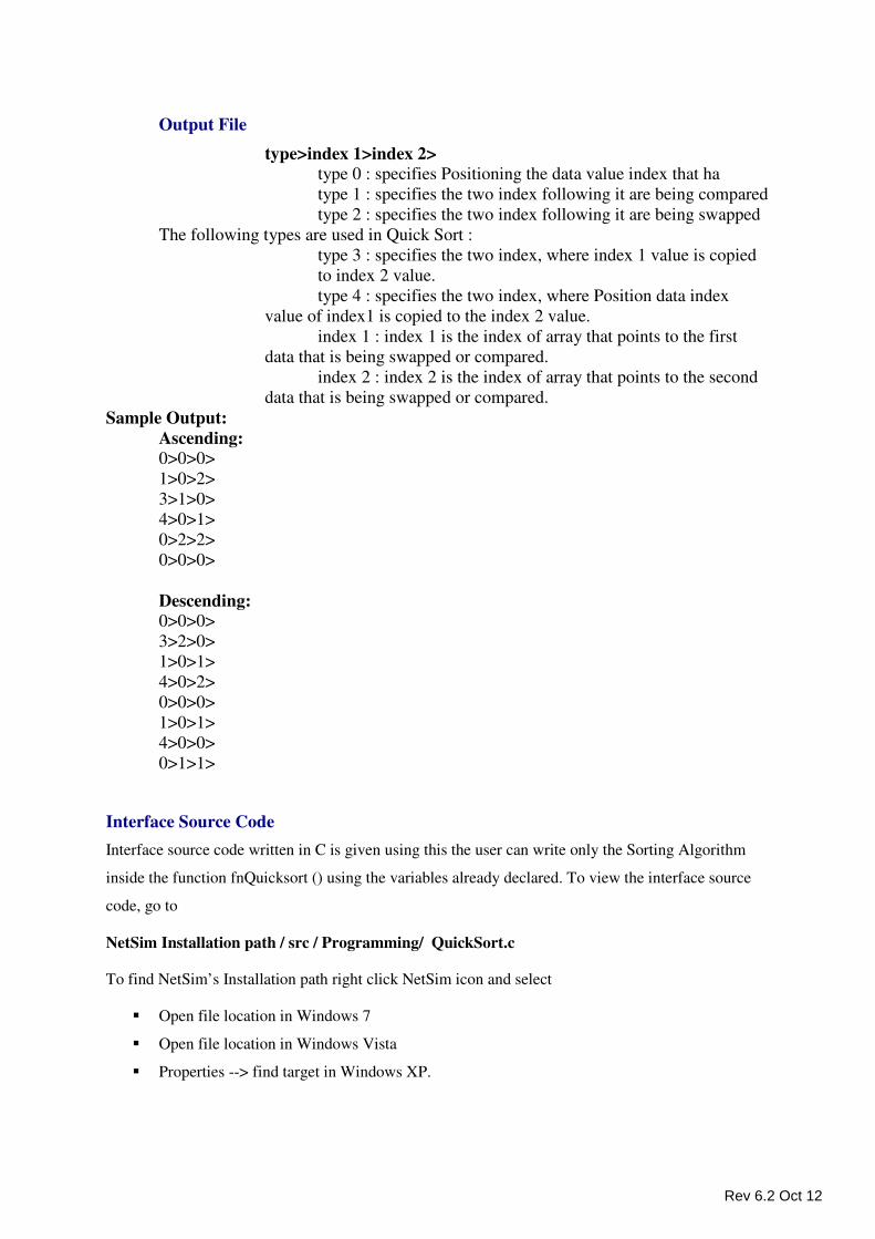
Output File
type>index 1>index 2> type 0 : specifies Positioning the data value index that ha
type 1 : specifies the two index following it are being compared
type 2 : specifies the two index following it are being swapped
The following types are used in Quick Sort :
type 3 : specifies the two index, where index 1 value is copied
to index 2 value.
type 4 : specifies the two index, where Position data index
value of index1 is copied to the index 2 value.
index 1 : index 1 is the index of array that points to the first
data that is being swapped or compared.
index 2 : index 2 is the index of array that points to the second
data that is being swapped or compared.
Sample Output:
Ascending: 0>0>0>
1>0>2>
3>1>0>
4>0>1>
0>2>2>
0>0>0>
Descending: 0>0>0>
3>2>0>
1>0>1>
4>0>2>
0>0>0>
1>0>1>
4>0>0>
0>1>1>
Interface Source Code
Interface source code written in C is given using this the user can write only the Sorting Algorithm
inside the function fnQuicksort () using the variables already declared. To view the interface source
code, go to
NetSim Installation path / src / Programming/ QuickSort.c
To find NetSim’s Installation path right click NetSim icon and select
� Open file location in Windows 7
� Open file location in Windows Vista
� Properties --> find target in Windows XP.
Rev 6.2 Oct 12
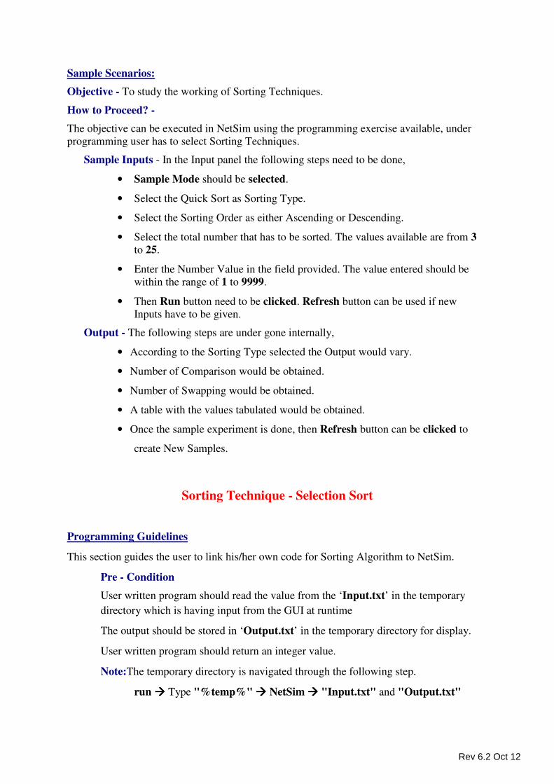
Sample Scenarios:
Objective - To study the working of Sorting Techniques.
How to Proceed? -
The objective can be executed in NetSim using the programming exercise available, under
programming user has to select Sorting Techniques.
Sample Inputs - In the Input panel the following steps need to be done,
• Sample Mode should be selected.
• Select the Quick Sort as Sorting Type.
• Select the Sorting Order as either Ascending or Descending.
• Select the total number that has to be sorted. The values available are from 3
to 25.
• Enter the Number Value in the field provided. The value entered should be
within the range of 1 to 9999.
• Then Run button need to be clicked. Refresh button can be used if new
Inputs have to be given.
Output - The following steps are under gone internally,
• According to the Sorting Type selected the Output would vary.
• Number of Comparison would be obtained.
• Number of Swapping would be obtained.
• A table with the values tabulated would be obtained.
• Once the sample experiment is done, then Refresh button can be clicked to
create New Samples.
Sorting Technique - Selection Sort
Programming Guidelines
This section guides the user to link his/her own code for Sorting Algorithm to NetSim.
Pre - Condition
User written program should read the value from the ‘Input.txt’ in the temporary
directory which is having input from the GUI at runtime
The output should be stored in ‘Output.txt’ in the temporary directory for display.
User written program should return an integer value.
Note:The temporary directory is navigated through the following step.
run ���� Type "%temp%" ���� NetSim ���� "Input.txt" and "Output.txt"
Rev 6.2 Oct 12
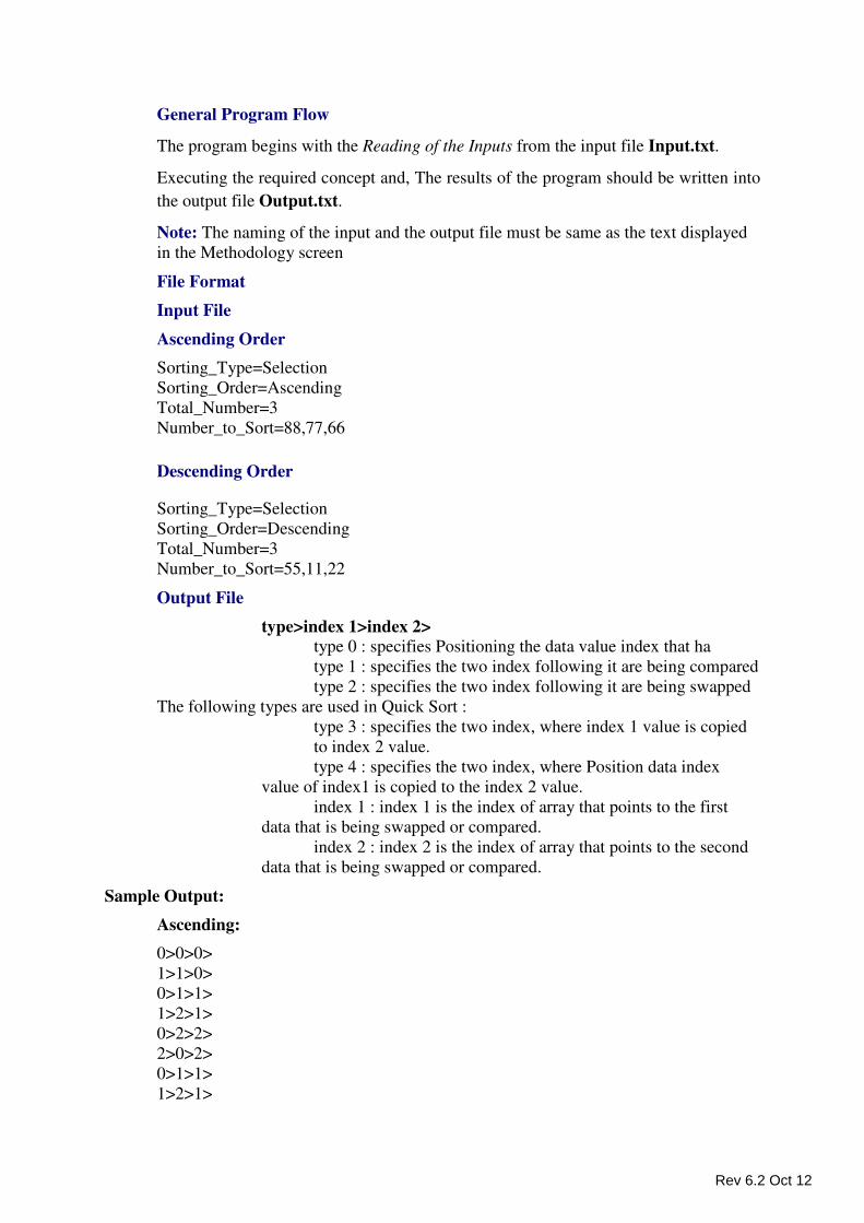
General Program Flow
The program begins with the Reading of the Inputs from the input file Input.txt.
Executing the required concept and, The results of the program should be written into
the output file Output.txt.
Note: The naming of the input and the output file must be same as the text displayed
in the Methodology screen
File Format
Input File
Ascending Order
Sorting_Type=Selection
Sorting_Order=Ascending
Total_Number=3
Number_to_Sort=88,77,66
Descending Order
Sorting_Type=Selection
Sorting_Order=Descending
Total_Number=3
Number_to_Sort=55,11,22
Output File
type>index 1>index 2> type 0 : specifies Positioning the data value index that ha
type 1 : specifies the two index following it are being compared
type 2 : specifies the two index following it are being swapped
The following types are used in Quick Sort :
type 3 : specifies the two index, where index 1 value is copied
to index 2 value.
type 4 : specifies the two index, where Position data index
value of index1 is copied to the index 2 value.
index 1 : index 1 is the index of array that points to the first
data that is being swapped or compared.
index 2 : index 2 is the index of array that points to the second
data that is being swapped or compared.
Sample Output:
Ascending:
0>0>0>
1>1>0>
0>1>1>
1>2>1>
0>2>2>
2>0>2>
0>1>1>
1>2>1>
Rev 6.2 Oct 12
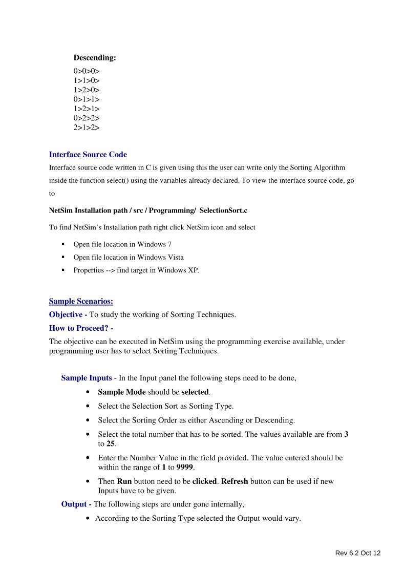
Descending:
0>0>0>
1>1>0>
1>2>0>
0>1>1>
1>2>1>
0>2>2>
2>1>2>
Interface Source Code
Interface source code written in C is given using this the user can write only the Sorting Algorithm
inside the function select() using the variables already declared. To view the interface source code, go
to
NetSim Installation path / src / Programming/ SelectionSort.c
To find NetSim’s Installation path right click NetSim icon and select
� Open file location in Windows 7
� Open file location in Windows Vista
� Properties --> find target in Windows XP.
Sample Scenarios:
Objective - To study the working of Sorting Techniques.
How to Proceed? -
The objective can be executed in NetSim using the programming exercise available, under
programming user has to select Sorting Techniques.
Sample Inputs - In the Input panel the following steps need to be done,
• Sample Mode should be selected.
• Select the Selection Sort as Sorting Type.
• Select the Sorting Order as either Ascending or Descending.
• Select the total number that has to be sorted. The values available are from 3
to 25.
• Enter the Number Value in the field provided. The value entered should be
within the range of 1 to 9999.
• Then Run button need to be clicked. Refresh button can be used if new
Inputs have to be given.
Output - The following steps are under gone internally,
• According to the Sorting Type selected the Output would vary.
Rev 6.2 Oct 12
• Number of Comparison would be obtained.
• Number of Swapping would be obtained.
• A table with the values tabulated would be obtained.
• Once the sample experiment is done, then Refresh button can be clicked to
create New Samples.
Spanning Tree – Borovska
Programming Guidelines
This section guides the user to link his/her own code for Spanning Tree using Borovska
algorithm to NetSim.
Pre - Conditions
The user program should read the input scenario from text file named ‘Input’ with
extension txt.
The user program after executing the concept should write the required output to a file
named ‘Output’ with extension txt.
Note:
The temporary directory is navigated through the following step.
run ���� Type "%temp%" ���� NetSim ���� "Input.txt" and "Output.txt"
General Program Flow
The program begins with the Reading of the Inputs from the input file Input.txt.
Executing the required concept and
The results of the program should be written into the output file Output.txt.
Input File Format
Algorithm=Borovska
No_of_Switches=3
No_of_Edges=3
Source_Switch=3,Destination_Switch=1,Distance=11,
Source_Switch=1,Destination_Switch=2,Distance=22,
Source_Switch=3,Destination_Switch=2,Distance=33,
Output File Format
‘Output.txt ’ file has the edges in the spanning tree, which is selected from the input
edges.
Node1>Node2>Cost> Example:
1>2>22>
1>3>11>
Rev 6.2 Oct 12
Interface Source Code
Interface source code written in C is given .Using this the user can write only the Borovska
algorithm inside the function fnBorovska() using the variables already declared. To view the
interface source code, go to
NetSim Installation path / src / Programming/ Boruvska.c
To find NetSim’s Installation path right click NetSim icon and select
� Open file location in Windows 7
� Open file location in Windows Vista
� Properties --> find target in Windows XP.
Sample Scenarios:
Objective - To find a Spanning Tree for a network using Borovska’s algorithm.
How to Proceed? - The objective can be executed in NetSim using the programming
exercise available. In the Programming Menu select Spanning Tree.
Sample Input
• Sample Mode should be selected.
• Select Borovska as Algorithm from the list available.
• Select the Number of Switches. Select 4 Switches as an Input.
• Click on 2 Switches to give the distance between them. Similarly connect all the
Switches that are available in the network. The Distances between the Routers
that needs to be given are as follows,
o Switch 1 and Switch 2 � 67 Km
o Switch 1 and Switch 4 � 46 Km
o Switch 1 and Switch 3 � 89 Km
o Switch 2 and Switch 3 � 78 Km
o Switch 2 and Switch 4 � 99 Km
o Switch 3 and Switch 4 � 56 Km
• Click on Run button to execute. Refresh button can be used if new Inputs have
to be given.
Sample Output
• The Spanning Tree Table with the Path (Source Switch and Destination
Switch) and Distance is obtained. Below is the Table that is obtained for the
above inputs,
Rev 6.2 Oct 12
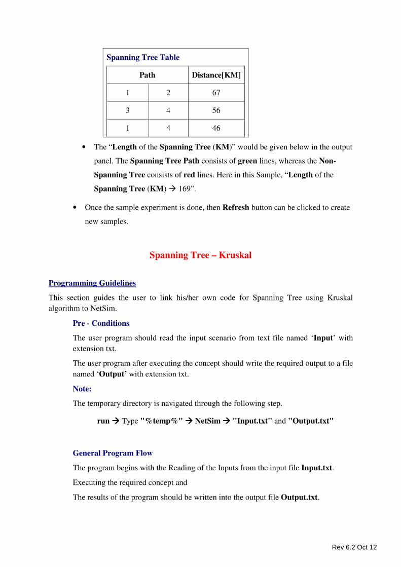
Spanning Tree Table
Path Distance[KM]
1 2 67
3 4 56
1 4 46
• The “Length of the Spanning Tree (KM)” would be given below in the output
panel. The Spanning Tree Path consists of green lines, whereas the Non-
Spanning Tree consists of red lines. Here in this Sample, “Length of the
Spanning Tree (KM) � 169”.
• Once the sample experiment is done, then Refresh button can be clicked to create
new samples.
Spanning Tree – Kruskal
Programming Guidelines
This section guides the user to link his/her own code for Spanning Tree using Kruskal
algorithm to NetSim.
Pre - Conditions
The user program should read the input scenario from text file named ‘Input’ with
extension txt.
The user program after executing the concept should write the required output to a file
named ‘Output’ with extension txt.
Note:
The temporary directory is navigated through the following step.
run ���� Type "%temp%" ���� NetSim ���� "Input.txt" and "Output.txt"
General Program Flow
The program begins with the Reading of the Inputs from the input file Input.txt.
Executing the required concept and
The results of the program should be written into the output file Output.txt.
Rev 6.2 Oct 12
Input File Format
Algorithm=Kruskal's
No_of_Switches=3
No_of_Edges=3
Source_Switch=3,Destination_Switch=1,Distance=23,
Source_Switch=1,Destination_Switch=2,Distance=34,
Source_Switch=3,Destination_Switch=2,Distance=45,
Output File Format
‘Output.txt ’ file has the edges in the spanning tree, which is selected from the input
edges.
Node1>Node2>Cost>
Example: 3>1>23>
1>2>34>
Interface Source Code
Interface source code written in C is given .Using this the user can write only the Kruskal
algorithm inside the function fnKruskal() using the variables already declared. To view the
interface source code, go to
NetSim Installation path / src / Programming/ Kruskal.c
To find NetSim’s Installation path right click NetSim icon and select
� Open file location in Windows 7
� Open file location in Windows Vista
� Properties --> find target in Windows XP.
Sample Scenarios:
Objective - To find the Spanning Tree for a network by using Kruskal algorithm.
How to Proceed? - The objective can be executed in NetSim using the programming
exercise available. In the Programming Menu select Spanning Tree.
Sample Input
• Sample Mode should be selected.
• Select Kruskal as Algorithm from the list available.
• Select the Number of Switches. Select 4 Switches as an Input.
• Click on 2 Switches to give the distance between them. Similarly connect all the
Switches that are available in the network. The Distances between the Routers
that needs to be given are as follows,
Rev 6.2 Oct 12
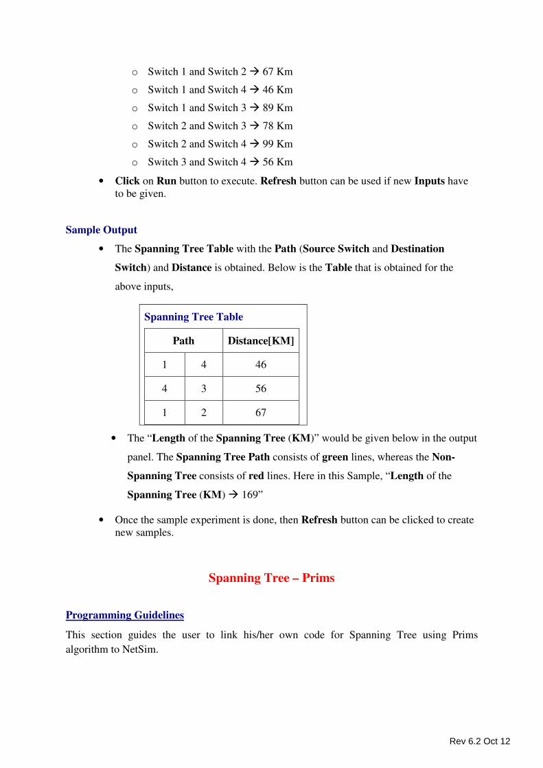
o Switch 1 and Switch 2 � 67 Km
o Switch 1 and Switch 4 � 46 Km
o Switch 1 and Switch 3 � 89 Km
o Switch 2 and Switch 3 � 78 Km
o Switch 2 and Switch 4 � 99 Km
o Switch 3 and Switch 4 � 56 Km
• Click on Run button to execute. Refresh button can be used if new Inputs have
to be given.
Sample Output
• The Spanning Tree Table with the Path (Source Switch and Destination
Switch) and Distance is obtained. Below is the Table that is obtained for the
above inputs,
Spanning Tree Table
Path Distance[KM]
1 4 46
4 3 56
1 2 67
• The “Length of the Spanning Tree (KM)” would be given below in the output
panel. The Spanning Tree Path consists of green lines, whereas the Non-
Spanning Tree consists of red lines. Here in this Sample, “Length of the
Spanning Tree (KM) � 169”
• Once the sample experiment is done, then Refresh button can be clicked to create
new samples.
Spanning Tree – Prims
Programming Guidelines
This section guides the user to link his/her own code for Spanning Tree using Prims
algorithm to NetSim.
Rev 6.2 Oct 12
Pre - Conditions
The user program should read the input scenario from text file named ‘Input’ with
extension txt.
The user program after executing the concept should write the required output to a file
named ‘Output’ with extension txt.
Note:
The temporary directory is navigated through the following step.
run ���� Type "%temp%" ���� NetSim ���� "Input.txt" and "Output.txt"
General Program Flow
The program begins with the Reading of the Inputs from the input file Input.txt.
Executing the required concept and
The results of the program should be written into the output file Output.txt.
Input File Format
Algorithm=Prim's
No_of_Switches=3
No_of_Edges=3
Source_Switch=1
Source_Switch=3,Destination_Switch=1,Distance=44,
Source_Switch=1,Destination_Switch=2,Distance=55,
Source_Switch=2,Destination_Switch=3,Distance=66,
Output File Format
‘Output.txt’ file has the edges in the spanning tree, which is selected from the input
edges.
Node1>Node2>Cost>
Example: 1>3>44>
1>2>55>
Interface Source Code
Interface source code written in C is given .Using this the user can write only the Prim’s
algorithm inside the function fnPrims() using the variables already declared. To view the
interface source code, go to
NetSim Installation path / src / Programming/ Prims.c
Rev 6.2 Oct 12
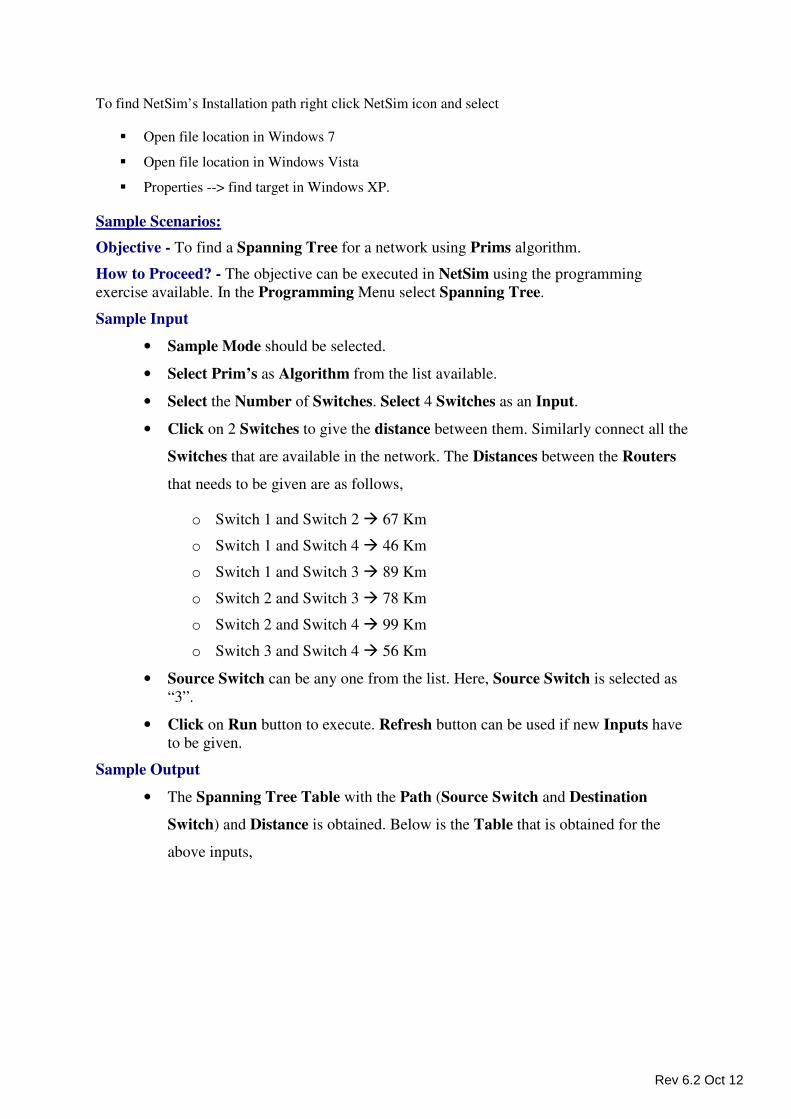
To find NetSim’s Installation path right click NetSim icon and select
� Open file location in Windows 7
� Open file location in Windows Vista
� Properties --> find target in Windows XP.
Sample Scenarios:
Objective - To find a Spanning Tree for a network using Prims algorithm.
How to Proceed? - The objective can be executed in NetSim using the programming
exercise available. In the Programming Menu select Spanning Tree.
Sample Input
• Sample Mode should be selected.
• Select Prim’s as Algorithm from the list available.
• Select the Number of Switches. Select 4 Switches as an Input.
• Click on 2 Switches to give the distance between them. Similarly connect all the
Switches that are available in the network. The Distances between the Routers
that needs to be given are as follows,
o Switch 1 and Switch 2 � 67 Km
o Switch 1 and Switch 4 � 46 Km
o Switch 1 and Switch 3 � 89 Km
o Switch 2 and Switch 3 � 78 Km
o Switch 2 and Switch 4 � 99 Km
o Switch 3 and Switch 4 � 56 Km
• Source Switch can be any one from the list. Here, Source Switch is selected as
“3”.
• Click on Run button to execute. Refresh button can be used if new Inputs have
to be given.
Sample Output
• The Spanning Tree Table with the Path (Source Switch and Destination
Switch) and Distance is obtained. Below is the Table that is obtained for the
above inputs,
Rev 6.2 Oct 12
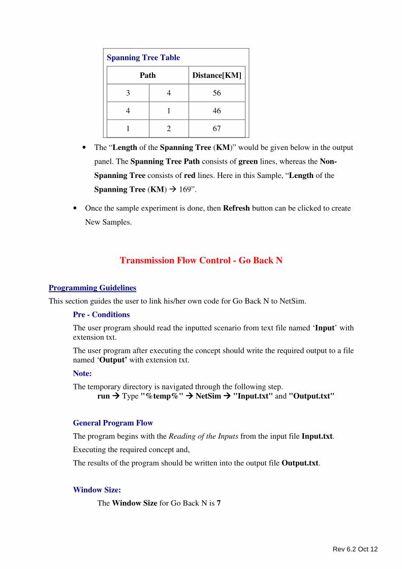
Spanning Tree Table
Path Distance[KM]
3 4 56
4 1 46
1 2 67
• The “Length of the Spanning Tree (KM)” would be given below in the output
panel. The Spanning Tree Path consists of green lines, whereas the Non-
Spanning Tree consists of red lines. Here in this Sample, “Length of the
Spanning Tree (KM) � 169”.
• Once the sample experiment is done, then Refresh button can be clicked to create
New Samples.
Transmission Flow Control - Go Back N
Programming Guidelines
This section guides the user to link his/her own code for Go Back N to NetSim.
Pre - Conditions
The user program should read the inputted scenario from text file named ‘Input’ with
extension txt.
The user program after executing the concept should write the required output to a file
named ‘Output’ with extension txt.
Note:
The temporary directory is navigated through the following step.
run ���� Type "%temp%" ���� NetSim ���� "Input.txt" and "Output.txt"
General Program Flow
The program begins with the Reading of the Inputs from the input file Input.txt.
Executing the required concept and,
The results of the program should be written into the output file Output.txt.
Window Size:
The Window Size for Go Back N is 7
Rev 6.2 Oct 12
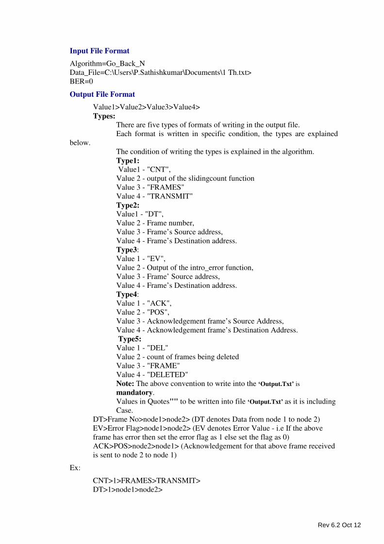
Input File Format
Algorithm=Go_Back_N
Data_File=C:\Users\P.Sathishkumar\Documents\1 Th.txt>
BER=0
Output File Format
Value1>Value2>Value3>Value4>
Types: There are five types of formats of writing in the output file.
Each format is written in specific condition, the types are explained
below.
The condition of writing the types is explained in the algorithm.
Type1: Value1 - "CNT",
Value 2 - output of the slidingcount function
Value 3 - "FRAMES"
Value 4 - "TRANSMIT"
Type2: Value1 - "DT",
Value 2 - Frame number,
Value 3 - Frame’s Source address,
Value 4 - Frame’s Destination address.
Type3:
Value 1 - "EV",
Value 2 - Output of the intro_error function,
Value 3 - Frame’ Source address,
Value 4 - Frame’s Destination address.
Type4:
Value 1 - "ACK",
Value 2 - "POS",
Value 3 - Acknowledgement frame’s Source Address,
Value 4 - Acknowledgement frame’s Destination Address.
Type5:
Value 1 - "DEL"
Value 2 - count of frames being deleted
Value 3 - "FRAME"
Value 4 - "DELETED"
Note: The above convention to write into the ‘Output.Txt’ is
mandatory.
Values in Quotes"" to be written into file ‘Output.Txt’ as it is including
Case.
DT>Frame No>node1>node2> (DT denotes Data from node 1 to node 2)
EV>Error Flag>node1>node2> (EV denotes Error Value - i.e If the above
frame has error then set the error flag as 1 else set the flag as 0)
ACK>POS>node2>node1> (Acknowledgement for that above frame received
is sent to node 2 to node 1)
Ex:
CNT>1>FRAMES>TRANSMIT>
DT>1>node1>node2>
Rev 6.2 Oct 12
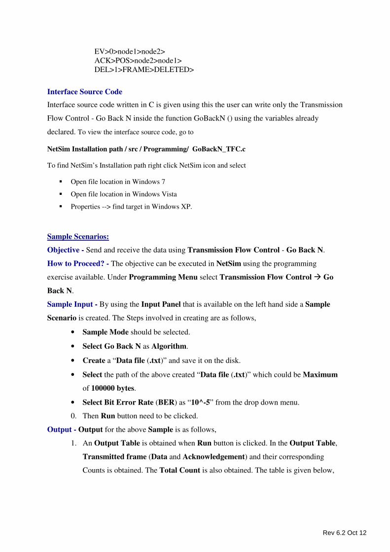
EV>0>node1>node2>
ACK>POS>node2>node1>
DEL>1>FRAME>DELETED>
Interface Source Code
Interface source code written in C is given using this the user can write only the Transmission
Flow Control - Go Back N inside the function GoBackN () using the variables already
declared. To view the interface source code, go to
NetSim Installation path / src / Programming/ GoBackN_TFC.c
To find NetSim’s Installation path right click NetSim icon and select
� Open file location in Windows 7
� Open file location in Windows Vista
� Properties --> find target in Windows XP.
Sample Scenarios:
Objective - Send and receive the data using Transmission Flow Control - Go Back N.
How to Proceed? - The objective can be executed in NetSim using the programming
exercise available. Under Programming Menu select Transmission Flow Control � Go
Back N.
Sample Input - By using the Input Panel that is available on the left hand side a Sample
Scenario is created. The Steps involved in creating are as follows,
• Sample Mode should be selected.
• Select Go Back N as Algorithm.
• Create a “Data file (.txt)” and save it on the disk.
• Select the path of the above created “Data file (.txt)” which could be Maximum
of 100000 bytes.
• Select Bit Error Rate (BER) as “10^-5” from the drop down menu.
0. Then Run button need to be clicked.
Output - Output for the above Sample is as follows,
1. An Output Table is obtained when Run button is clicked. In the Output Table,
Transmitted frame (Data and Acknowledgement) and their corresponding
Counts is obtained. The Total Count is also obtained. The table is given below,
Rev 6.2 Oct 12
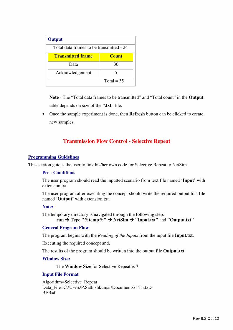
Output
Total data frames to be transmitted - 24
Transmitted frame Count
Data 30
Acknowledgement 5
Total = 35
Note - The “Total data frames to be transmitted” and “Total count” in the Output
table depends on size of the “.txt” file.
• Once the sample experiment is done, then Refresh button can be clicked to create
new samples.
Transmission Flow Control - Selective Repeat
Programming Guidelines
This section guides the user to link his/her own code for Selective Repeat to NetSim.
Pre - Conditions
The user program should read the inputted scenario from text file named ‘Input’ with
extension txt.
The user program after executing the concept should write the required output to a file
named ‘Output’ with extension txt.
Note:
The temporary directory is navigated through the following step.
run ���� Type "%temp%" ���� NetSim ���� "Input.txt" and "Output.txt"
General Program Flow
The program begins with the Reading of the Inputs from the input file Input.txt.
Executing the required concept and,
The results of the program should be written into the output file Output.txt.
Window Size:
The Window Size for Selective Repeat is 7
Input File Format
Algorithm=Selective_Repeat
Data_File=C:\Users\P.Sathishkumar\Documents\1 Th.txt>
BER=0
Rev 6.2 Oct 12
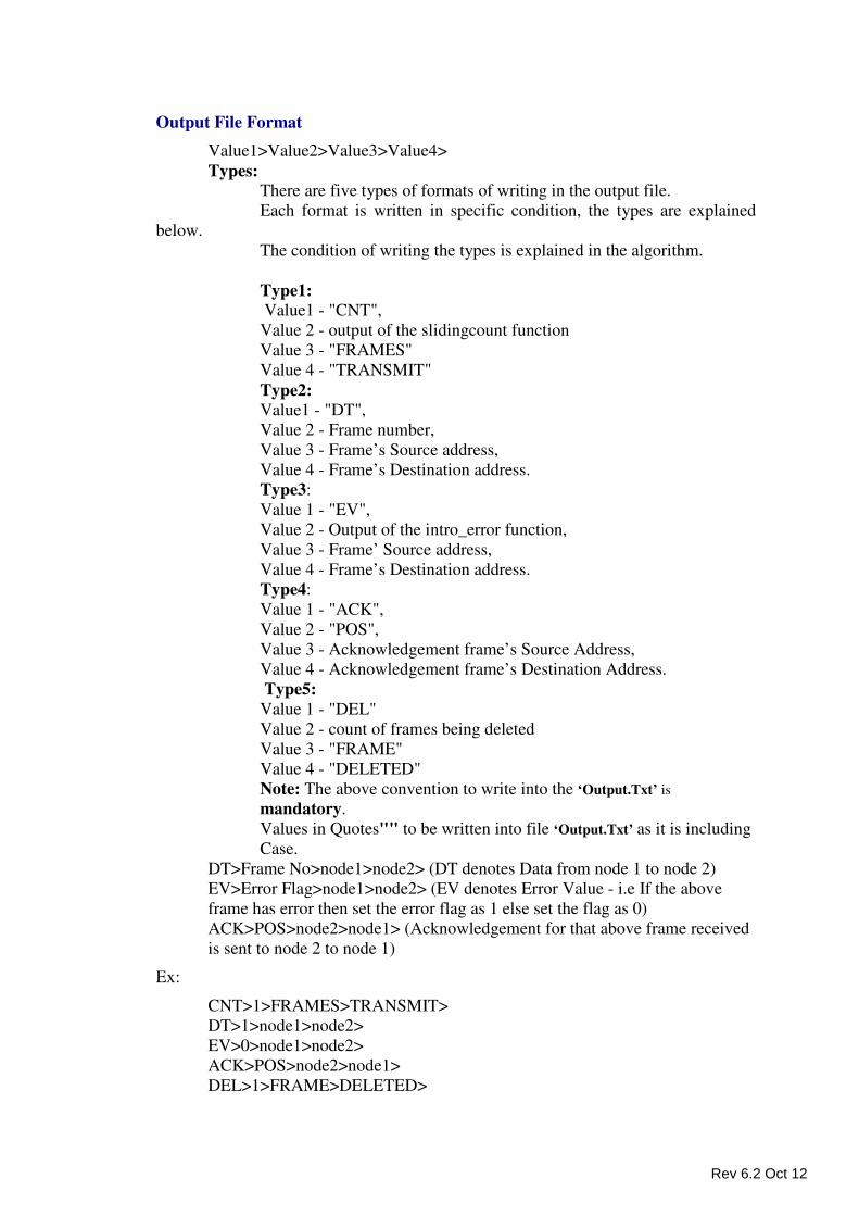
Output File Format
Value1>Value2>Value3>Value4>
Types: There are five types of formats of writing in the output file.
Each format is written in specific condition, the types are explained
below.
The condition of writing the types is explained in the algorithm.
Type1: Value1 - "CNT",
Value 2 - output of the slidingcount function
Value 3 - "FRAMES"
Value 4 - "TRANSMIT"
Type2: Value1 - "DT",
Value 2 - Frame number,
Value 3 - Frame’s Source address,
Value 4 - Frame’s Destination address.
Type3:
Value 1 - "EV",
Value 2 - Output of the intro_error function,
Value 3 - Frame’ Source address,
Value 4 - Frame’s Destination address.
Type4:
Value 1 - "ACK",
Value 2 - "POS",
Value 3 - Acknowledgement frame’s Source Address,
Value 4 - Acknowledgement frame’s Destination Address.
Type5:
Value 1 - "DEL"
Value 2 - count of frames being deleted
Value 3 - "FRAME"
Value 4 - "DELETED"
Note: The above convention to write into the ‘Output.Txt’ is
mandatory.
Values in Quotes"" to be written into file ‘Output.Txt’ as it is including
Case.
DT>Frame No>node1>node2> (DT denotes Data from node 1 to node 2)
EV>Error Flag>node1>node2> (EV denotes Error Value - i.e If the above
frame has error then set the error flag as 1 else set the flag as 0)
ACK>POS>node2>node1> (Acknowledgement for that above frame received
is sent to node 2 to node 1)
Ex:
CNT>1>FRAMES>TRANSMIT>
DT>1>node1>node2>
EV>0>node1>node2>
ACK>POS>node2>node1>
DEL>1>FRAME>DELETED>
Rev 6.2 Oct 12
Interface Source Code
Interface source code written in C is given using this the user can write only the Transmission
Flow Control -Selective Repeat inside the function SelectiveRepeat () using the variables
already declared. To view the interface source code, go to
NetSim Installation path / src / Programming/ SelectiveRepeat_TFC.c
To find NetSim’s Installation path right click NetSim icon and select
� Open file location in Windows 7
� Open file location in Windows Vista
� Properties --> find target in Windows XP.
Sample Scenarios:
Objective - Send and receive the data using Transmission Flow Control - Selective Repeat.
How to Proceed? - The objective can be executed in NetSim using the programming
exercise available. Under Programming Menu select Transmission Flow Control �
Selective Repeat.
Sample Input - By using the Input Panel that is available on the left hand side a Sample
Scenario is created. The Steps involved in creating are as follows,
• Sample Mode should be selected.
• Select Selective Repeat as Algorithm.
• Create a “Data file (.txt)” and save it on the disk.
• Select the path of the above created “Data file (.txt)” which could be Maximum
of 100000 bytes.
• Select Bit Error Rate (BER) as “10^-5” from the drop down menu.
0. Then Run button need to be clicked.
1.
Output - Output for the above Sample is as follows,
2. An Output Table is obtained when Run button is clicked. In the Output Table,
Transmitted frame (Data and Acknowledgement) and their corresponding
Counts is obtained. The Total Count is also obtained. The table is given below,
Rev 6.2 Oct 12
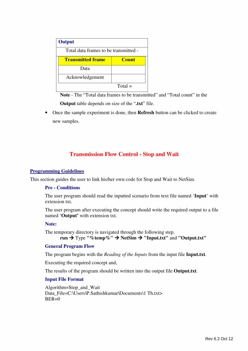
Output
Total data frames to be transmitted -
Transmitted frame Count
Data
Acknowledgement
Total =
Note - The “Total data frames to be transmitted” and “Total count” in the
Output table depends on size of the “.txt” file.
• Once the sample experiment is done, then Refresh button can be clicked to create
new samples.
Transmission Flow Control - Stop and Wait
Programming Guidelines
This section guides the user to link his/her own code for Stop and Wait to NetSim.
Pre - Conditions
The user program should read the inputted scenario from text file named ‘Input’ with
extension txt.
The user program after executing the concept should write the required output to a file
named ‘Output’ with extension txt.
Note:
The temporary directory is navigated through the following step.
run ���� Type "%temp%" ���� NetSim ���� "Input.txt" and "Output.txt"
General Program Flow
The program begins with the Reading of the Inputs from the input file Input.txt.
Executing the required concept and,
The results of the program should be written into the output file Output.txt.
Input File Format
Algorithm=Stop_and_Wait
Data_File=C:\Users\P.Sathishkumar\Documents\1 Th.txt>
BER=0
Rev 6.2 Oct 12
Output File Format Value1>Value2>Value3>Value4>
Types: There are five types of formats of writing in the output file.
Each format is written in specific condition, the types are explained
below.
The condition of writing the types is explained in the algorithm.
Type1: Value1 - "CNT",
Value 2 - output of the slidingcount function
Value 3 - "FRAMES"
Value 4 - "TRANSMIT"
Type2: Value1 - "DT",
Value 2 - Frame number,
Value 3 - Frame’s Source address,
Value 4 - Frame’s Destination address.
Type3:
Value 1 - "EV",
Value 2 - Output of the intro_error function,
Value 3 - Frame’ Source address,
Value 4 - Frame’s Destination address.
Type4:
Value 1 - "ACK",
Value 2 - "POS",
Value 3 - Acknowledgement frame’s Source Address,
Value 4 - Acknowledgement frame’s Destination Address.
Type5:
Value 1 - "DEL"
Value 2 - count of frames being deleted
Value 3 - "FRAME"
Value 4 - "DELETED"
Note: The above convention to write into the ‘Output.Txt’ is
mandatory.
Values in Quotes"" to be written into file ‘Output.Txt’ as it is including
Case.
DT>Frame No>node1>node2> (DT denotes Data from node 1 to node 2)
EV>Error Flag>node1>node2> (EV denotes Error Value - i.e If the above
frame has error then set the error flag as 1 else set the flag as 0)
ACK>POS>node2>node1> (Acknowledgement for that above frame received
is sent to node 2 to node 1)
Ex:
DT>1>node1>node2>
EV>0>node1>node2>
ACK>POS>node2>node1>
Rev 6.2 Oct 12
Interface Source Code
Interface source code written in C is given using this the user can write only the Transmission
Flow Control - Stop and Wait inside the function stopandwait() using the variables already
declared. To view the interface source code, go to
NetSim Installation path / src / Programming/ StopandWait.c
To find NetSim’s Installation path right click NetSim icon and select
� Open file location in Windows 7
� Open file location in Windows Vista
� Properties --> find target in Windows XP.
Sample Scenarios:
Objective - Send and receive the data using Transmission Flow Control– Stop and wait.
How to Proceed? - The objective can be executed in NetSim using the programming
exercise available. Under Programming Menu select Transmission Flow Control � Stop
and wait.
Sample Input - In the Input panel the following steps need to be done,
• Sample Mode should be selected.
• Stop and Wait needs to be selected for Algorithm.
• The path of the “Data file (.txt)” should be entered.
• Bit Error Rate (BER) should be selected.
• Then Run button need to be clicked. Refresh button can be used if new
Inputs have to be given.
Output - The following steps are under gone internally,
• When the Run Button is clicked the Tool generates the Output in the following
format,
Rev 6.2 Oct 12
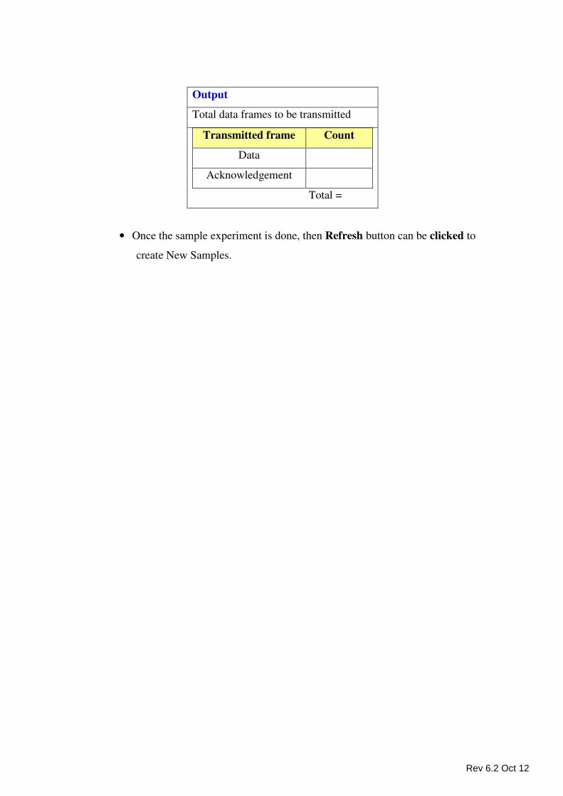
Output
Total data frames to be transmitted
Transmitted frame Count
Data
Acknowledgement
Total =
• Once the sample experiment is done, then Refresh button can be clicked to
create New Samples.
Rev 6.2 Oct 12
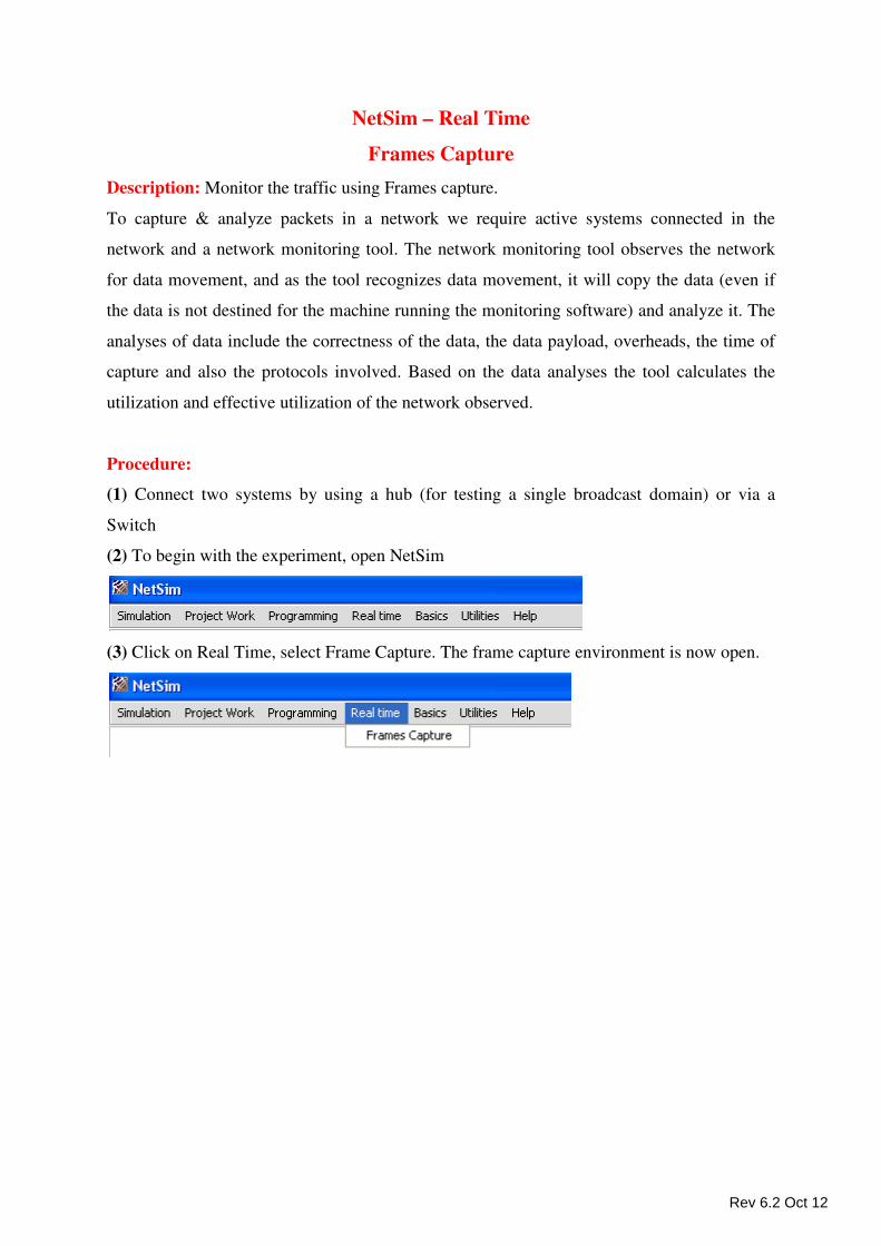
NetSim – Real Time
Frames Capture
Description: Monitor the traffic using Frames capture.
To capture & analyze packets in a network we require active systems connected in the
network and a network monitoring tool. The network monitoring tool observes the network
for data movement, and as the tool recognizes data movement, it will copy the data (even if
the data is not destined for the machine running the monitoring software) and analyze it. The
analyses of data include the correctness of the data, the data payload, overheads, the time of
capture and also the protocols involved. Based on the data analyses the tool calculates the
utilization and effective utilization of the network observed.
Procedure:
(1) Connect two systems by using a hub (for testing a single broadcast domain) or via a
Switch
(2) To begin with the experiment, open NetSim
(3) Click on Real Time, select Frame Capture. The frame capture environment is now open.
Rev 6.2 Oct 12
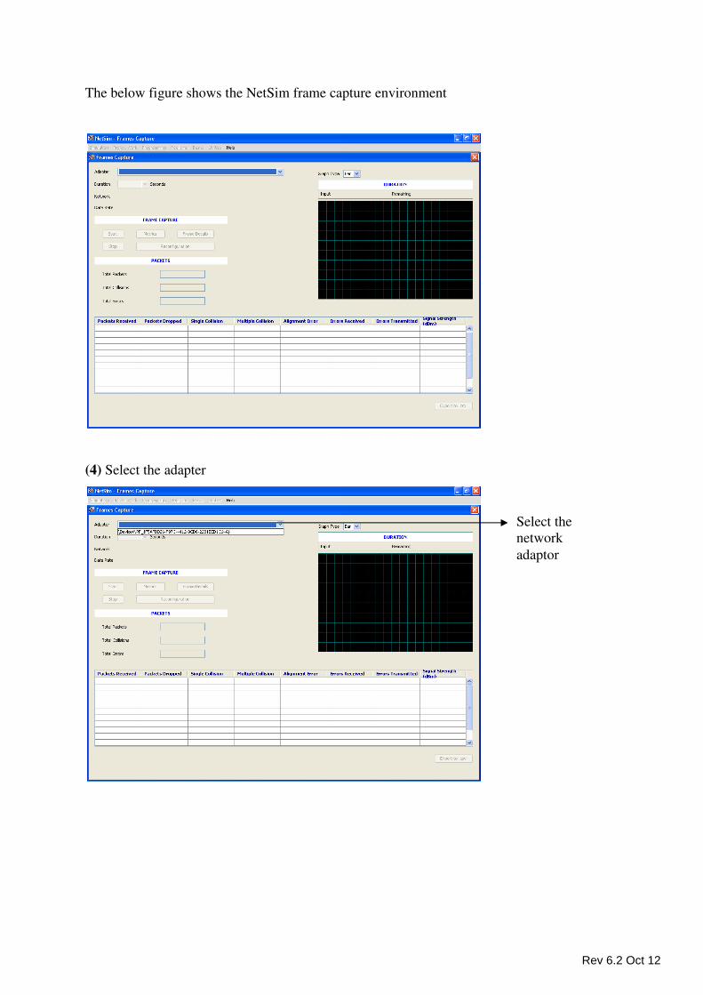
The below figure shows the NetSim frame capture environment
(4) Select the adapter
Select the
network
adaptor
Rev 6.2 Oct 12
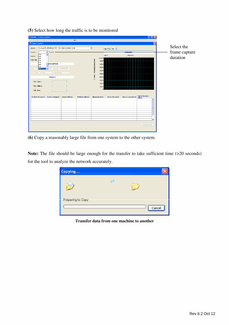
(5) Select how long the traffic is to be monitored
(6) Copy a reasonably large file from one system to the other system.
Note: The file should be large enough for the transfer to take sufficient time (>20 seconds)
for the tool to analyze the network accurately.
Transfer data from one machine to another
Select the
frame capture
duration
Rev 6.2 Oct 12
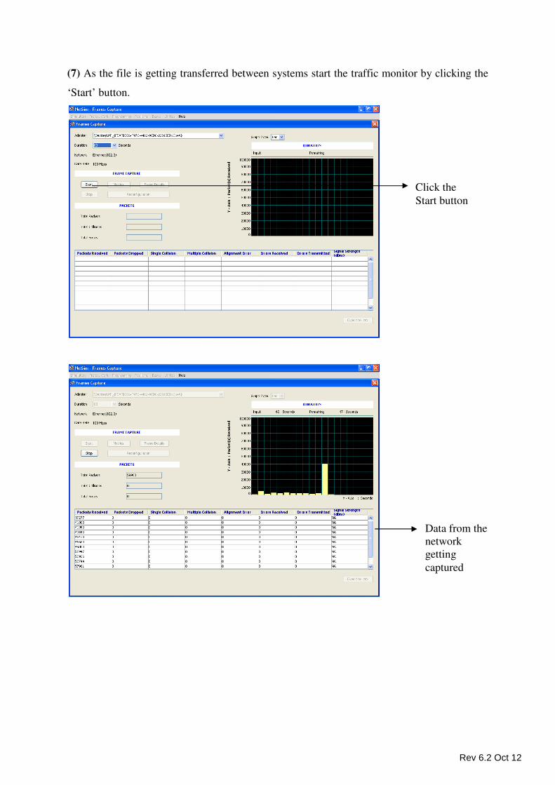
(7) As the file is getting transferred between systems start the traffic monitor by clicking the
‘Start’ button.
Click the
Start button
Data from the
network
getting
captured
Rev 6.2 Oct 12
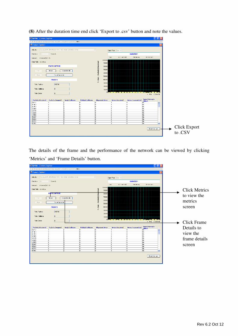
(8) After the duration time end click ‘Export to .csv’ button and note the values.
The details of the frame and the performance of the network can be viewed by clicking
‘Metrics’ and ‘Frame Details’ button.
Click Export
to .CSV
Click Metrics
to view the
metrics
screen
Click Frame
Details to
view the
frame details
screen
Rev 6.2 Oct 12
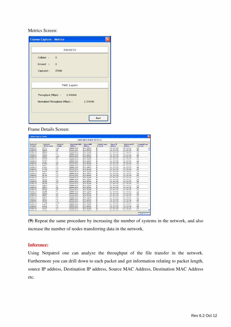
Metrics Screen:
Frame Details Screen:
(9) Repeat the same procedure by increasing the number of systems in the network, and also
increase the number of nodes transferring data in the network.
Inference:
Using Netpatrol one can analyze the throughput of the file transfer in the network.
Furthermore you can drill down to each packet and get information relating to packet length,
source IP address, Destination IP address, Source MAC Address, Destination MAC Address
etc.
Rev 6.2 Oct 12
NetSim - Utilities
User Management
Tasks such as Addition of new user, deletion of existing user, operational mode (Exam/Practice) of the user setting can be performed by using this menu. This module is available only to the Administrator.
The Administrator has to give the correct password and click on OK button to enter into the User Management interface. This is used for verification purpose. The buttons available in User Management window are,
• Add User - This button is used for creating new users. The following fields have to be filled in,
o Username - Name of the new user needs to be entered in the field provided.
o Category - By default student is selected.
o Mode - Either Practice / Exam mode needs to be selected.
o Click on Accept / Cancel button to accept / cancel the changes.
• Delete User - This button is used for deleting the existing users. The following options have to be filled in,
o Username - Name of the user needs to be entered in the field provided.
o Category - By default student is selected.
o Mode - Either Practice / Exam mode needs to be selected.
o Click on Accept / Cancel button to accept / cancel the changes.
• Change Mode - This button is used for changing the mode. There are two modes present in the software,
o Practice Mode - Students will be able to get all the help that is associated with the software. Saved experiments can be reused. If this mode is selected, then the user would have access to
1. Under Simulation all the saved experiments in Simulation when the user is in Practice mode can be “opened and reused”, “delete if they are not required” and “Saved experiment can be used in the Analytics interface”.
2. Under Programming Sample as well as User mode can be made use of. Also help document “Concepts, Algorithm, Pseudo Code and Flowchart” can be viewed.
3. Basics Menu,
4. NetSim Help.
o Exam Mode - Students will not be able to use the help associated with the software. Also saved experiments in the Practice mode cannot be reused in the Exam mode. If this mode is selected, then the user would have access to,
Rev 6.2 Oct 12
1. Under Simulation all the saved experiments in Simulation when the user is in Exam mode can be “opened and reused”, “delete if they are not required” and “Saved experiment can be used in the Analytics interface”.
2. Under Programming only User mode can be made use of. User will be restricted from using “Concepts, Algorithm, Pseudo Code and Flowchart”.
3. Basics Menu cannot be accessed,
4. NetSim Help can be used.
Rev 6.2 Oct 12


![HE ART OF THE UTILIZATION OF RAFFIC SIMULATION MODELS: … · NETSIM [NETSIM. WWW site], REST [Yoshida, et al. 1999], and SIPA [Yokochi, et al. 1999] along the verification manual](https://img.pdfslide.us/doc/110x75/5fbcf5a65c79e834b3039cc7/he-art-of-the-utilization-of-raffic-simulation-models-netsim-netsim-www-site.jpg)