University of Bristol

NERC Internship Report

Aerial Photogrammetry for theEarth Sciences

Author:Drew Silcock

Supervisor:Dr Juliet Biggs

Tuesday 7th October, 2014

1 Introduction

The aim of this project is to investigate the practical use of photogrammetry,with a focus of its applications to the Earth Sciences. It covers the methods usedto gain photogrammetric data and analyses some results taken from fieldwork.

1.1 How photogrammetry works

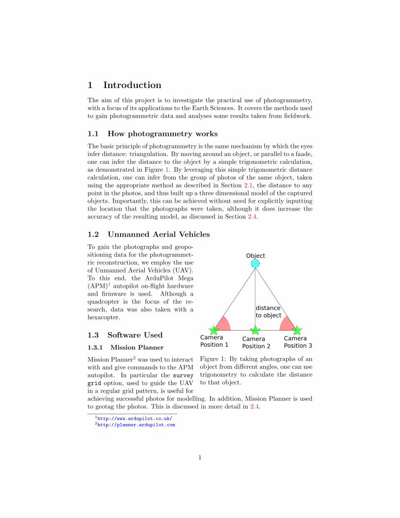
The basic principle of photogrammetry is the same mechanism by which the eyesinfer distance: triangulation. By moving around an object, or parallel to a faade,one can infer the distance to the object by a simple trigonometric calculation,as demonstrated in Figure 1. By leveraging this simple trigonometric distancecalculation, one can infer from the group of photos of the same object, takenusing the appropriate method as described in Section 2.1, the distance to anypoint in the photos, and thus built up a three dimensional model of the capturedobjects. Importantly, this can be achieved without need for explicitly inputtingthe location that the photographs were taken, although it does increase theaccuracy of the resulting model, as discussed in Section 2.4.

1.2 Unmanned Aerial Vehicles

Object

distanceto object

CameraPosition 1

CameraPosition 2

CameraPosition 3

Figure 1: By taking photographs of anobject from different angles, one can usetrigonometry to calculate the distanceto that object.

To gain the photographs and geopo-sitioning data for the photogrammet-ric reconstruction, we employ the useof Unmanned Aerial Vehicles (UAV).To this end, the ArduPilot Mega(APM)1 autopilot on-flight hardwareand firmware is used. Although aquadcopter is the focus of the re-search, data was also taken with ahexacopter.

1.3 Software Used

1.3.1 Mission Planner

Mission Planner2 was used to interactwith and give commands to the APMautopilot. In particular the survey

grid option, used to guide the UAVin a regular grid pattern, is useful forachieving successful photos for modelling. In addition, Mission Planner is usedto geotag the photos. This is discussed in more detail in 2.4.

1http://www.ardupilot.co.uk/2http://planner.ardupilot.com

1

1.3.2 Agisoft PhotoScan

The Agisoft PhotoScan Professional Edition software3 software is used to per-form the photogrammetric reconstruction. The workflow is as follows:

Load Photos Firstly, the photos are loaded in PhotoScan.

Load Camera Positions Then, the camera geotagging data are loaded, eitherthrough importing the photo exif metadata, or through a separate commaseparated value file.

Align Photos The camera positions are then used to refine the camera posi-tion and build a sparse point cloud.

Place Ground Control Points Next a mesh is generated and the GCPs areinput into PhotoScan.

Optimise alignment The camera alignment is then optimised using the GCPdata.

Build Dense Point Cloud PhotoScan subsequently builds a dense point cloudfrom the sparse point cloud.

Build Mesh Penultimately, the mesh is built by joining the dense point cloudinto a smooth model.

Build Texture Finally, the mesh is overlaid with a texture, finished the pho-togrammetric reconstruction.

Once this workflow is accomplished, the resulting model can be exported asan orthophoto, whereby the original photos are stitched together into a singleaerial image, and as a Digital Elevation Model (DEM), which contains all theinformation about the topography of the model. It is this DEM that is ofapplication to Earth Science research.

1.3.3 Canon Hack Development Kit

In order to control the camera remotely, we employed the Canon Hack Devel-opment Kit (CHDK)4. Specifically, we used firmware version 1.00B Alpha forthe Powershot IXUS1325, loaded by a bootable SD card. This allows one to runscripts on the camera, written in either Lua or UBASIC, that interface with thecamera mechanism, e.g. taking pictures, zooming, turning off etc. This allowedus control over the camera during the flights.

3http://www.agisoft.ru/products/photoscan/professional/4http://chdk.wikia.com/5http://chdk.wikia.com/wiki/ELPH115

2

2 Methods

2.1 Photographic Technique

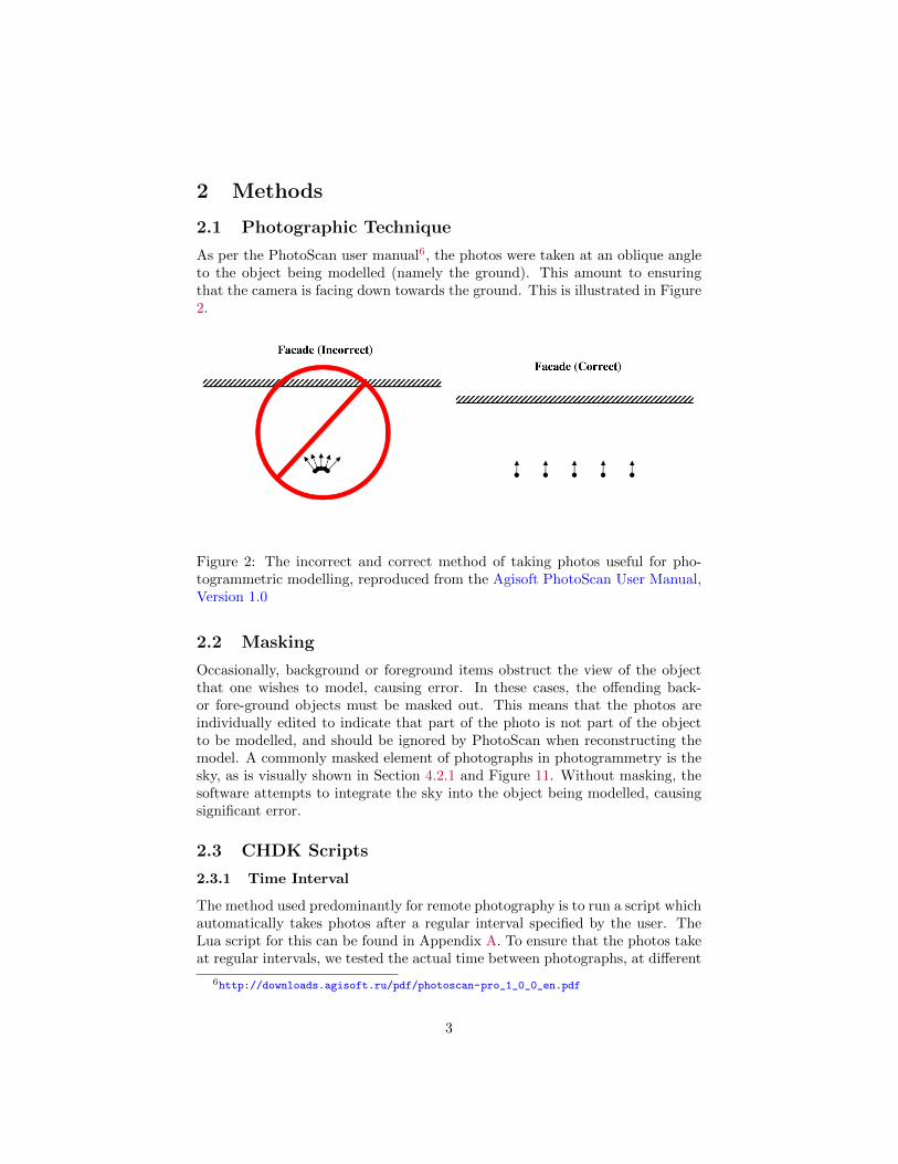
As per the PhotoScan user manual6, the photos were taken at an oblique angleto the object being modelled (namely the ground). This amount to ensuringthat the camera is facing down towards the ground. This is illustrated in Figure2.

Figure 2: The incorrect and correct method of taking photos useful for pho-togrammetric modelling, reproduced from the Agisoft PhotoScan User Manual,Version 1.0

2.2 Masking

Occasionally, background or foreground items obstruct the view of the objectthat one wishes to model, causing error. In these cases, the offending back-or fore-ground objects must be masked out. This means that the photos areindividually edited to indicate that part of the photo is not part of the objectto be modelled, and should be ignored by PhotoScan when reconstructing themodel. A commonly masked element of photographs in photogrammetry is thesky, as is visually shown in Section 4.2.1 and Figure 11. Without masking, thesoftware attempts to integrate the sky into the object being modelled, causingsignificant error.

2.3 CHDK Scripts

2.3.1 Time Interval

The method used predominantly for remote photography is to run a script whichautomatically takes photos after a regular interval specified by the user. TheLua script for this can be found in Appendix A. To ensure that the photos takeat regular intervals, we tested the actual time between photographs, at different

6http://downloads.agisoft.ru/pdf/photoscan-pro_1_0_0_en.pdf

3

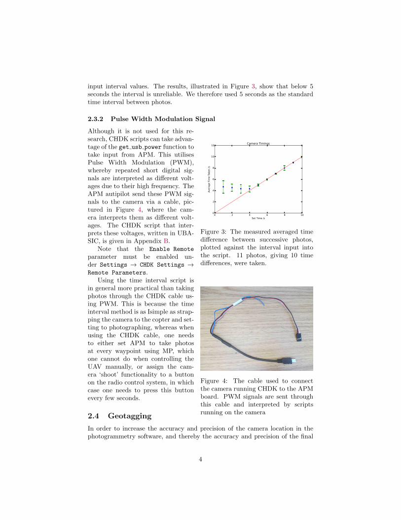
input interval values. The results, illustrated in Figure 3, show that below 5seconds the interval is unreliable. We therefore used 5 seconds as the standardtime interval between photos.

2.3.2 Pulse Width Modulation Signal

Set Time s

AverageTim

eTaken

s

Camera Timings

Figure 3: The measured averaged timedifference between successive photos,plotted against the interval input intothe script. 11 photos, giving 10 timedifferences, were taken.

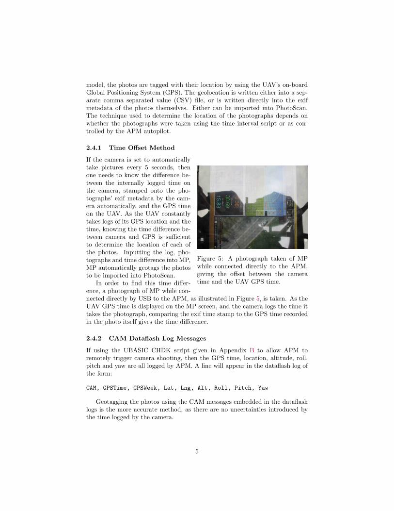
Although it is not used for this re-search, CHDK scripts can take advan-tage of the get usb power function totake input from APM. This utilisesPulse Width Modulation (PWM),whereby repeated short digital sig-nals are interpreted as different volt-ages due to their high frequency. TheAPM autipilot send these PWM sig-nals to the camera via a cable, pic-tured in Figure 4, where the cam-era interprets them as different volt-ages. The CHDK script that inter-prets these voltages, written in UBA-SIC, is given in Appendix B.

Note that the Enable Remote

parameter must be enabled un-der Settings → CHDK Settings →Remote Parameters.

Figure 4: The cable used to connectthe camera running CHDK to the APMboard. PWM signals are sent throughthis cable and interpreted by scriptsrunning on the camera

Using the time interval script isin general more practical than takingphotos through the CHDK cable us-ing PWM. This is because the timeinterval method is as Isimple as strap-ping the camera to the copter and set-ting to photographing, whereas whenusing the CHDK cable, one needsto either set APM to take photosat every waypoint using MP, whichone cannot do when controlling theUAV manually, or assign the cam-era ‘shoot’ functionality to a buttonon the radio control system, in whichcase one needs to press this buttonevery few seconds.

2.4 Geotagging

In order to increase the accuracy and precision of the camera location in thephotogrammetry software, and thereby the accuracy and precision of the final

4

model, the photos are tagged with their location by using the UAV’s on-boardGlobal Positioning System (GPS). The geolocation is written either into a sep-arate comma separated value (CSV) file, or is written directly into the exifmetadata of the photos themselves. Either can be imported into PhotoScan.The technique used to determine the location of the photographs depends onwhether the photographs were taken using the time interval script or as con-trolled by the APM autopilot.

2.4.1 Time Offset Method

Figure 5: A photograph taken of MPwhile connected directly to the APM,giving the offset between the cameratime and the UAV GPS time.

If the camera is set to automaticallytake pictures every 5 seconds, thenone needs to know the difference be-tween the internally logged time onthe camera, stamped onto the pho-tographs’ exif metadata by the cam-era automatically, and the GPS timeon the UAV. As the UAV constantlytakes logs of its GPS location and thetime, knowing the time difference be-tween camera and GPS is sufficientto determine the location of each ofthe photos. Inputting the log, pho-tographs and time difference into MP,MP automatically geotags the photosto be imported into PhotoScan.

In order to find this time differ-ence, a photograph of MP while con-nected directly by USB to the APM, as illustrated in Figure 5, is taken. As theUAV GPS time is displayed on the MP screen, and the camera logs the time ittakes the photograph, comparing the exif time stamp to the GPS time recordedin the photo itself gives the time difference.

2.4.2 CAM Dataflash Log Messages

If using the UBASIC CHDK script given in Appendix B to allow APM toremotely trigger camera shooting, then the GPS time, location, altitude, roll,pitch and yaw are all logged by APM. A line will appear in the dataflash log ofthe form:

CAM, GPSTime, GPSWeek, Lat, Lng, Alt, Roll, Pitch, Yaw

Geotagging the photos using the CAM messages embedded in the dataflashlogs is the more accurate method, as there are no uncertainties introduced bythe time logged by the camera.

5

2.4.3 Shutter Lag

If using the CAM message method, the lag between the instruction to shootand the photograph being actually taken, induced by shutter lag, can causesystematic errors in the geotagging and must be measured so that it can be takeninto account. To quantify this, we analysed the shutter lag of the PowershotIXUS132 we are using. This involved taking a photo of a timer7 exactly onthe second, and noting the time shown in the photograph. We calculated theshutter lag to be (90.3 ± 32.0)ms excluding the autofocus lag, and (341 ±140.3)ms including the autofocus lag. As the camera is not set to autofocususing this method of remote photography, the former value is taken as the valueof interest. As the GPS logs are made only at a frequency of 5 Hz (or one every200 ms)8, the shutter lag is rounded to the nearest 200 ms and taken as zero.

2.5 Ground Control Points

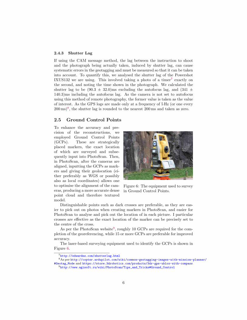
Figure 6: The equipment used to surveyin Ground Control Points.

To enhance the accuracy and pre-cision of the reconstructions, weemployed Ground Control Points(GCPs). These are strategicallyplaced markers, the exact locationof which are surveyed and subse-quently input into PhotoScan. Then,in PhotoScan, after the cameras arealigned, inputting the GCPs as mark-ers and giving their geolocation (ei-ther preferably as WGS or possiblyalso as local coordinates) allows oneto optimise the alignment of the cam-eras, producing a more accurate densepoint cloud and therefore texturedmodel.

Distinguishable points such as dark crosses are preferable, as they are eas-ier to pick out on photos when creating markers in PhotoScan, and easier forPhotoScan to analyse and pick out the location of in each picture. I particularcrosses are effective as the exact location of the marker can be precisely set tothe centre of the cross.

As per the PhotoScan website9, roughly 10 GCPs are required for the com-pletion of the georeferencing, while 15 or more GCPs are preferable for improvedaccuracy.

The laser-based surveying equipment used to identify the GCPs is shown inFigure 6.

7http://edwardns.com/shutterlag.html8As per http://copter.ardupilot.com/wiki/common-geotagging-images-with-mission-planner/

#Geotag_Mode and https://store.3drobotics.com/products/3dr-gps-ublox-with-compass9http://www.agisoft.ru/wiki/PhotoScan/Tips_and_Tricks#Ground_Control

6

Camera

Ground

Heig

ht,

h

Distance photographed, x

αx

HORIZONTAL(a) The horizontal view of the angle ofview of the camera facing the ground.

Camera

Distance photographed, y

Ground

Heig

ht,

h

αy

VERTICAL(b) The vertical view of the angle of viewof the camera facing the ground.

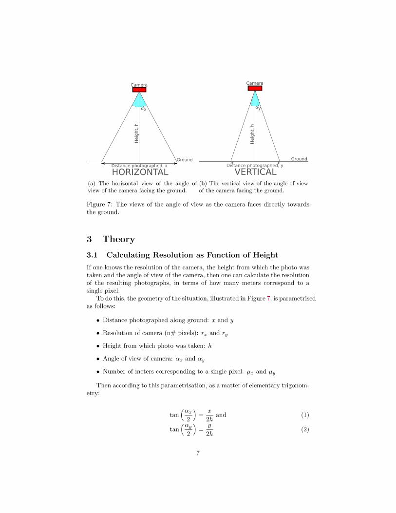
Figure 7: The views of the angle of view as the camera faces directly towardsthe ground.

3 Theory

3.1 Calculating Resolution as Function of Height

If one knows the resolution of the camera, the height from which the photo wastaken and the angle of view of the camera, then one can calculate the resolutionof the resulting photographs, in terms of how many meters correspond to asingle pixel.

To do this, the geometry of the situation, illustrated in Figure 7, is parametrisedas follows:

• Distance photographed along ground: x and y

• Resolution of camera (n# pixels): rx and ry

• Height from which photo was taken: h

• Angle of view of camera: αx and αy

• Number of meters corresponding to a single pixel: µx and µy

Then according to this parametrisation, as a matter of elementary trigonom-etry:

tan(αx

2

)=

x

2hand (1)

tan(αy

2

)=

y

2h(2)

7

Rearranging this for x and y gives:

x = 2h tan(αx

2

)and (3)

y = 2h tan(αy

2

)(4)

Then the resolution in meters per pixel is simply this distance x divided bythe total number of pixels in the photograph:

µx =x

rx=

2h tan(αx

2

)rx

and (5)

µy =y

ry=

2h tan(αy

2

)ry

(6)

This agrees approximately with the values generated by PhotoScan in doingthe photogrammetric reconstruction, discussed in Sections 4.1.2 and 4.2.3.

3.2 Ensuring sufficient photo overlap

Agisoft states in the PhotoScan User Manual10 that 80% overlap is needed forstandard front overlap between successive photos. Thus, one can calculate thespeed one needs to travel at to ensure that if one takes photos every five seconds,the overlap is at least 80%.

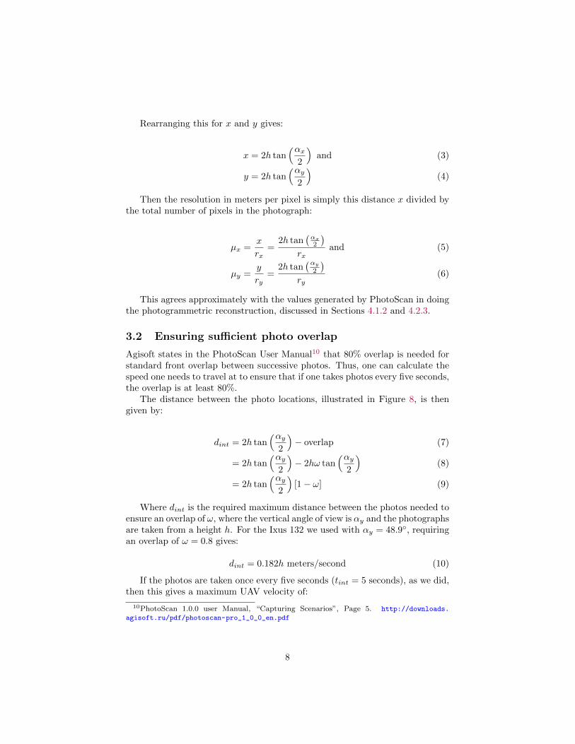
The distance between the photo locations, illustrated in Figure 8, is thengiven by:

dint = 2h tan(αy

2

)− overlap (7)

= 2h tan(αy

2

)− 2hω tan

(αy2

)(8)

= 2h tan(αy

2

)[1− ω] (9)

Where dint is the required maximum distance between the photos needed toensure an overlap of ω, where the vertical angle of view is αy and the photographsare taken from a height h. For the Ixus 132 we used with αy = 48.9◦, requiringan overlap of ω = 0.8 gives:

dint = 0.182h meters/second (10)

If the photos are taken once every five seconds (tint = 5 seconds), as we did,then this gives a maximum UAV velocity of:

10PhotoScan 1.0.0 user Manual, “Capturing Scenarios”, Page 5. http://downloads.

agisoft.ru/pdf/photoscan-pro_1_0_0_en.pdf

8

Overlap

Distance between photos

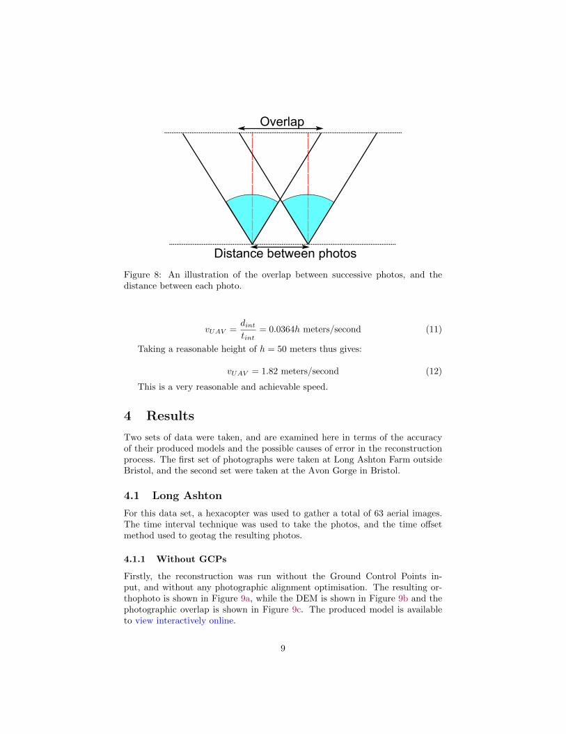
Figure 8: An illustration of the overlap between successive photos, and thedistance between each photo.

vUAV =dinttint

= 0.0364h meters/second (11)

Taking a reasonable height of h = 50 meters thus gives:

vUAV = 1.82 meters/second (12)

This is a very reasonable and achievable speed.

4 Results

Two sets of data were taken, and are examined here in terms of the accuracyof their produced models and the possible causes of error in the reconstructionprocess. The first set of photographs were taken at Long Ashton Farm outsideBristol, and the second set were taken at the Avon Gorge in Bristol.

4.1 Long Ashton

For this data set, a hexacopter was used to gather a total of 63 aerial images.The time interval technique was used to take the photos, and the time offsetmethod used to geotag the resulting photos.

4.1.1 Without GCPs

Firstly, the reconstruction was run without the Ground Control Points in-put, and without any photographic alignment optimisation. The resulting or-thophoto is shown in Figure 9a, while the DEM is shown in Figure 9b and thephotographic overlap is shown in Figure 9c. The produced model is availableto view interactively online.

9

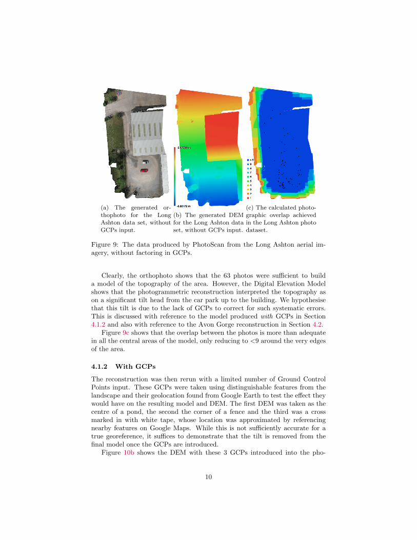
(a) The generated or-thophoto for the LongAshton data set, withoutGCPs input.

(b) The generated DEMfor the Long Ashton dataset, without GCPs input.

(c) The calculated photo-graphic overlap achievedin the Long Ashton photodataset.

Figure 9: The data produced by PhotoScan from the Long Ashton aerial im-agery, without factoring in GCPs.

Clearly, the orthophoto shows that the 63 photos were sufficient to builda model of the topography of the area. However, the Digital Elevation Modelshows that the photogrammetric reconstruction interpreted the topography ason a significant tilt head from the car park up to the building. We hypothesisethat this tilt is due to the lack of GCPs to correct for such systematic errors.This is discussed with reference to the model produced with GCPs in Section4.1.2 and also with reference to the Avon Gorge reconstruction in Section 4.2.

Figure 9c shows that the overlap between the photos is more than adequatein all the central areas of the model, only reducing to <9 around the very edgesof the area.

4.1.2 With GCPs

The reconstruction was then rerun with a limited number of Ground ControlPoints input. These GCPs were taken using distinguishable features from thelandscape and their geolocation found from Google Earth to test the effect theywould have on the resulting model and DEM. The first DEM was taken as thecentre of a pond, the second the corner of a fence and the third was a crossmarked in with white tape, whose location was approximated by referencingnearby features on Google Maps. While this is not sufficiently accurate for atrue georeference, it suffices to demonstrate that the tilt is removed from thefinal model once the GCPs are introduced.

Figure 10b shows the DEM with these 3 GCPs introduced into the pho-

10

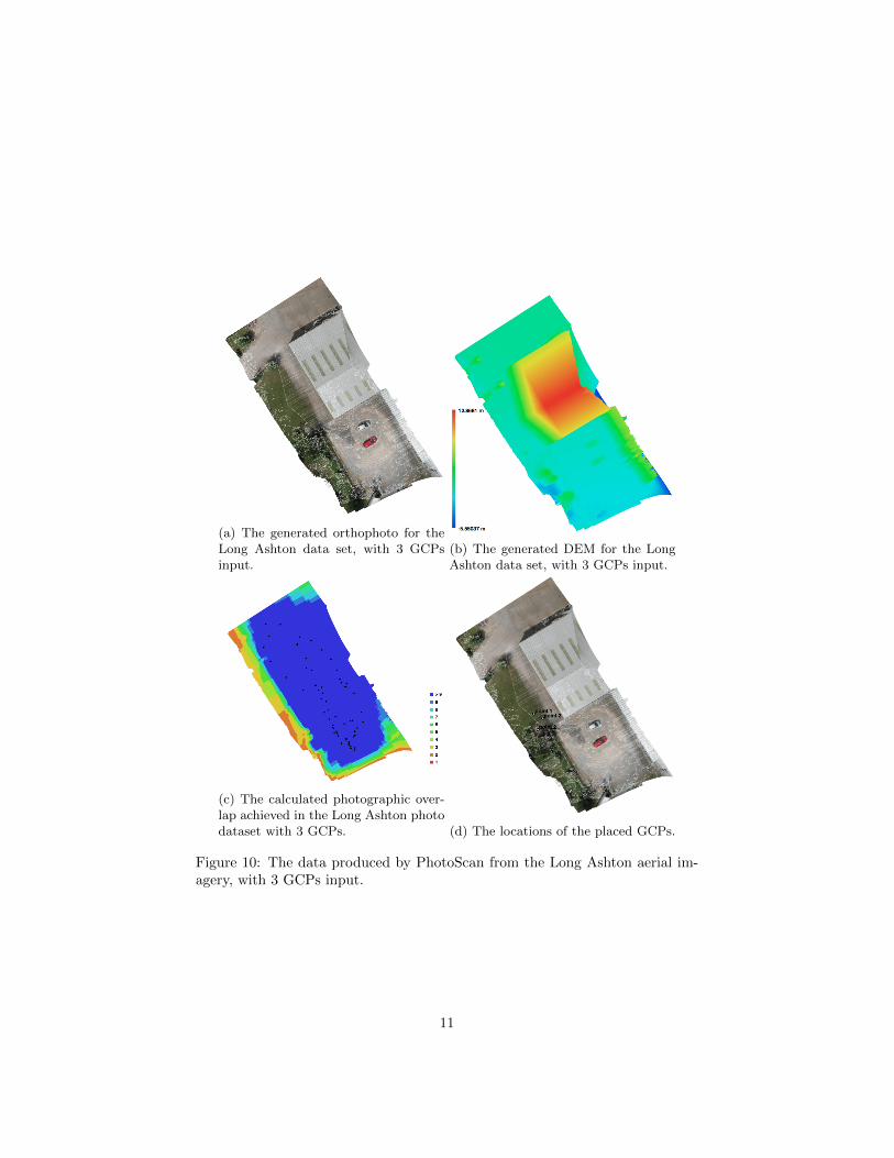
(a) The generated orthophoto for theLong Ashton data set, with 3 GCPsinput.

(b) The generated DEM for the LongAshton data set, with 3 GCPs input.

(c) The calculated photographic over-lap achieved in the Long Ashton photodataset with 3 GCPs. (d) The locations of the placed GCPs.

Figure 10: The data produced by PhotoScan from the Long Ashton aerial im-agery, with 3 GCPs input.

11

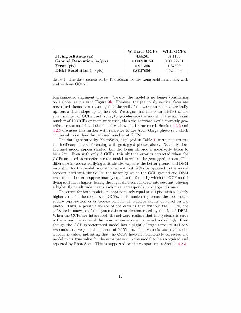
Without GCPs With GCPsFlying Altitude (m) 4.88261 37.1183Ground Resolution (m/pix) 0.000940159 0.00622731Error (pix) 0.971366 1.37699DEM Resolution (m/pix) 0.00376064 0.0249093

Table 1: The data generated by PhotoScan for the Long Ashton models, withand without GCPs.

togrammetric alignment process. Clearly, the model is no longer consideringon a slope, as it was in Figure 9b. However, the previously vertical faces arenow tilted themselves, meaning that the wall of the warehouse is not verticallyup, but a tilted slope up to the roof. We argue that this is an artefact of thesmall number of GCPs used trying to georeference the model. If the minimumnumber of 10 GCPs or more were used, then the software would correctly geo-reference the model and the sloped walls would be corrected. Section 4.2.2 and4.2.3 discusses this further with reference to the Avon Gorge photo set, whichcontained more than the required number of GCPs.

The data generated by PhotoScan, displayed in Table 1, further illustratesthe inefficacy of georeferencing with geotagged photos alone. Not only doesthe final model appear slanted, but the flying altitude is incorrectly taken tobe 4.9 m. Even with only 3 GCPs, this altitude error is corrected when theGCPs are used to georeference the model as well as the geotagged photos. Thisdifference in calculated flying altitude also explains the better ground and DEMresolution for the model reconstructed without GCPs as opposed to the modelreconstructed with the GCPs; the factor by which the GCP ground and DEMresolution is better is approximately equal to the factor by which the GCP modelflying altitude is higher, taking the slight difference in error into account. Havinga higher flying altitude means each pixel corresponds to a larger distance.

The errors for both models are approximately equal at≈ 1 pix, with a slightlyhigher error for the model with GCPs. This number represents the root meanssquare reprojection error calculated over all features points detected on thephoto. Thus, a possible source of the error is that without the GCPs, thesoftware in unaware of the systematic error demonstrated by the sloped DEM.When the GCPs are introduced, the software realises that the systematic erroris there, and the value of the reprojection error is increased accordingly. Eventhough the GCP georeferenced model has a slightly larger error, it still cor-responds to a very small distance of 0.155 mm. This value is too small to bea realistic value, indicating that the GCPs have not sufficiently corrected themodel to its true value for the error present in the model to be recognised andreported by PhotoScan. This is supported by the comparison in Section 4.2.3.

12

4.2 Avon Gorge

This model was reconstructed from two passes of 87 and 61 photos. As before,the time interval with time offset techniques were used for taking photos andgeotagging the photos, respectively. The photos were taken by attaching thecamera to the quadcopter and tilting it by hand to attain horizontally orientedphotographs of the cliff face that is the Avon-Gorge. The purpose of this was togive useful photos equivalent to aerial photogrammetry before the quadcopterwas ready to fly.

4.2.1 First Pass Versus Second Pass

The first pass was taken facing the gorge horizontally on, thereby fully repre-senting an equivalent to aerial photogrammetry. The second pass was at anoblique angle, facing upwards to capture the top of the gorge. As expected, thesecond pass at an oblique angle produced less accurate results than the firstpass a zenithal angle to the cliff face. This is shown visually in Figures 11a and11b. In particular where the oblique angle causes the camera to be unable tosee the top of the cliff and where the cliff meets the sky, the model is erroneous.For the former the model produces clear spikes in the model, jutting from theface of the cliff. For the latter, the software includes the sky as an extension ofthe cliff. Masking the sky out, as described in Section 2.2, removes the latterproblem to a limited extent, but the former remains, as shown in Figure 11c.

4.2.2 Without GCPs

When the first pass is taken with no GCPs input, there are several importantemergent features to note.

Firstly, as Figure 12d shows, the calculated locations of the cameras was veryinaccurate, with some errors extending beyond the model. This is because thegeolocation of the photos from the on-board UAV GPS is simply not accurateenough to be the only method of georeferencing; the GCPs are also needed inaddition to the geotagged photo locations.

Secondly, as Figure 12b shows, the reconstruction has also incorrectly in-terpreted the landscape as being on a tilt, with the north of the gorge (top ofthe image) appearing higher than the south of the gorge (bottom of the image).The systematic sloping that these reconstructions seem to exhibit is a strange ifirrelevant phenomenon (so long as a sufficient number of GCPs are provided),possibly caused by the camera being tilted as it is attached to the UAVs.

4.2.3 With GCPs

Once the GCPs are input, there are several important effects.The photographic overlap of the gorge increases, with only the very corners

having less than 9 overlapped photos covering it. With more accurate georefer-encing, the software recognises the photos as taken more spread apart, and thuswith better coverage of the corners of the model.

13

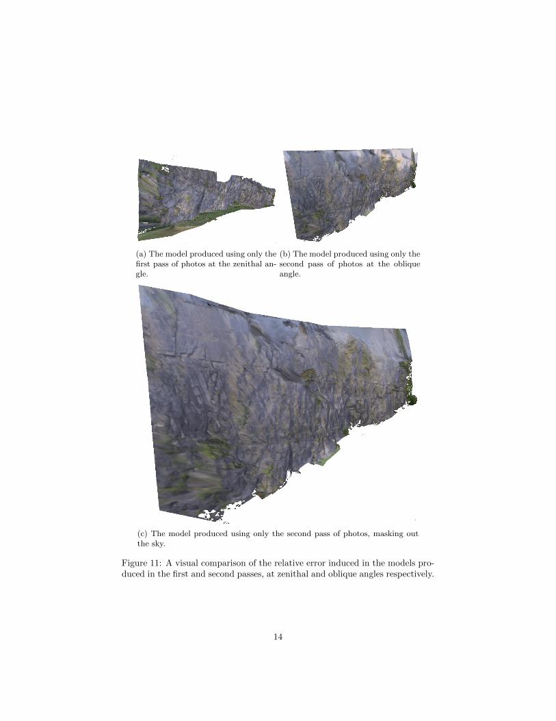
(a) The model produced using only thefirst pass of photos at the zenithal an-gle.

(b) The model produced using only thesecond pass of photos at the obliqueangle.

(c) The model produced using only the second pass of photos, masking outthe sky.

Figure 11: A visual comparison of the relative error induced in the models pro-duced in the first and second passes, at zenithal and oblique angles respectively.

14

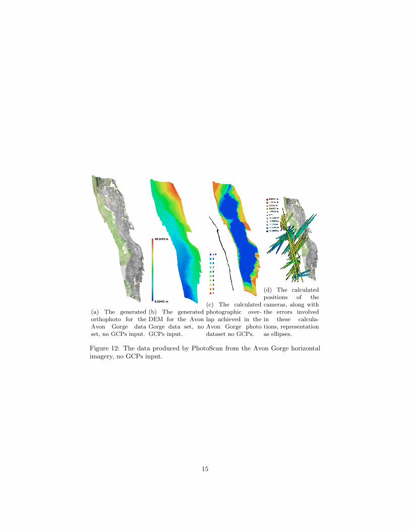
(a) The generatedorthophoto for theAvon Gorge dataset, no GCPs input.

(b) The generatedDEM for the AvonGorge data set, noGCPs input.

(c) The calculatedphotographic over-lap achieved in theAvon Gorge photodataset no GCPs.

(d) The calculatedpositions of thecameras, along withthe errors involvedin these calcula-tions, representationas ellipses.

Figure 12: The data produced by PhotoScan from the Avon Gorge horizontalimagery, no GCPs input.

15

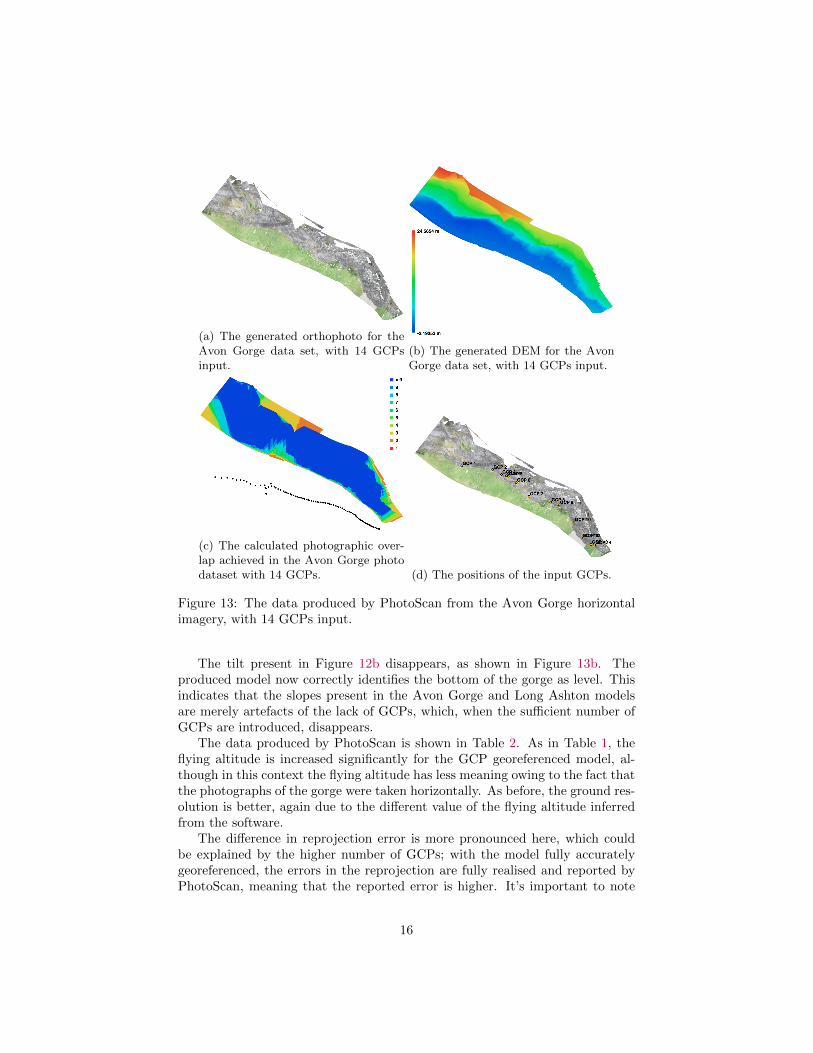
(a) The generated orthophoto for theAvon Gorge data set, with 14 GCPsinput.

(b) The generated DEM for the AvonGorge data set, with 14 GCPs input.

(c) The calculated photographic over-lap achieved in the Avon Gorge photodataset with 14 GCPs. (d) The positions of the input GCPs.

Figure 13: The data produced by PhotoScan from the Avon Gorge horizontalimagery, with 14 GCPs input.

The tilt present in Figure 12b disappears, as shown in Figure 13b. Theproduced model now correctly identifies the bottom of the gorge as level. Thisindicates that the slopes present in the Avon Gorge and Long Ashton modelsare merely artefacts of the lack of GCPs, which, when the sufficient number ofGCPs are introduced, disappears.

The data produced by PhotoScan is shown in Table 2. As in Table 1, theflying altitude is increased significantly for the GCP georeferenced model, al-though in this context the flying altitude has less meaning owing to the fact thatthe photographs of the gorge were taken horizontally. As before, the ground res-olution is better, again due to the different value of the flying altitude inferredfrom the software.

The difference in reprojection error is more pronounced here, which couldbe explained by the higher number of GCPs; with the model fully accuratelygeoreferenced, the errors in the reprojection are fully realised and reported byPhotoScan, meaning that the reported error is higher. It’s important to note

16

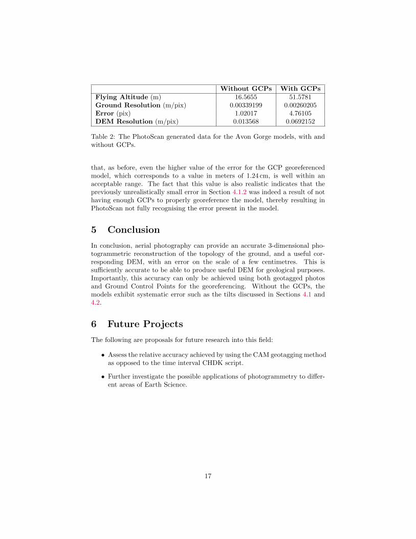
Without GCPs With GCPsFlying Altitude (m) 16.5655 51.5781Ground Resolution (m/pix) 0.00339199 0.00260205Error (pix) 1.02017 4.76105DEM Resolution (m/pix) 0.013568 0.0692152

Table 2: The PhotoScan generated data for the Avon Gorge models, with andwithout GCPs.

that, as before, even the higher value of the error for the GCP georeferencedmodel, which corresponds to a value in meters of 1.24 cm, is well within anacceptable range. The fact that this value is also realistic indicates that thepreviously unrealistically small error in Section 4.1.2 was indeed a result of nothaving enough GCPs to properly georeference the model, thereby resulting inPhotoScan not fully recognising the error present in the model.

5 Conclusion

In conclusion, aerial photography can provide an accurate 3-dimensional pho-togrammetric reconstruction of the topology of the ground, and a useful cor-responding DEM, with an error on the scale of a few centimetres. This issufficiently accurate to be able to produce useful DEM for geological purposes.Importantly, this accuracy can only be achieved using both geotagged photosand Ground Control Points for the georeferencing. Without the GCPs, themodels exhibit systematic error such as the tilts discussed in Sections 4.1 and4.2.

6 Future Projects

The following are proposals for future research into this field:

• Assess the relative accuracy achieved by using the CAM geotagging methodas opposed to the time interval CHDK script.

• Further investigate the possible applications of photogrammetry to differ-ent areas of Earth Science.

17

7 Appendices

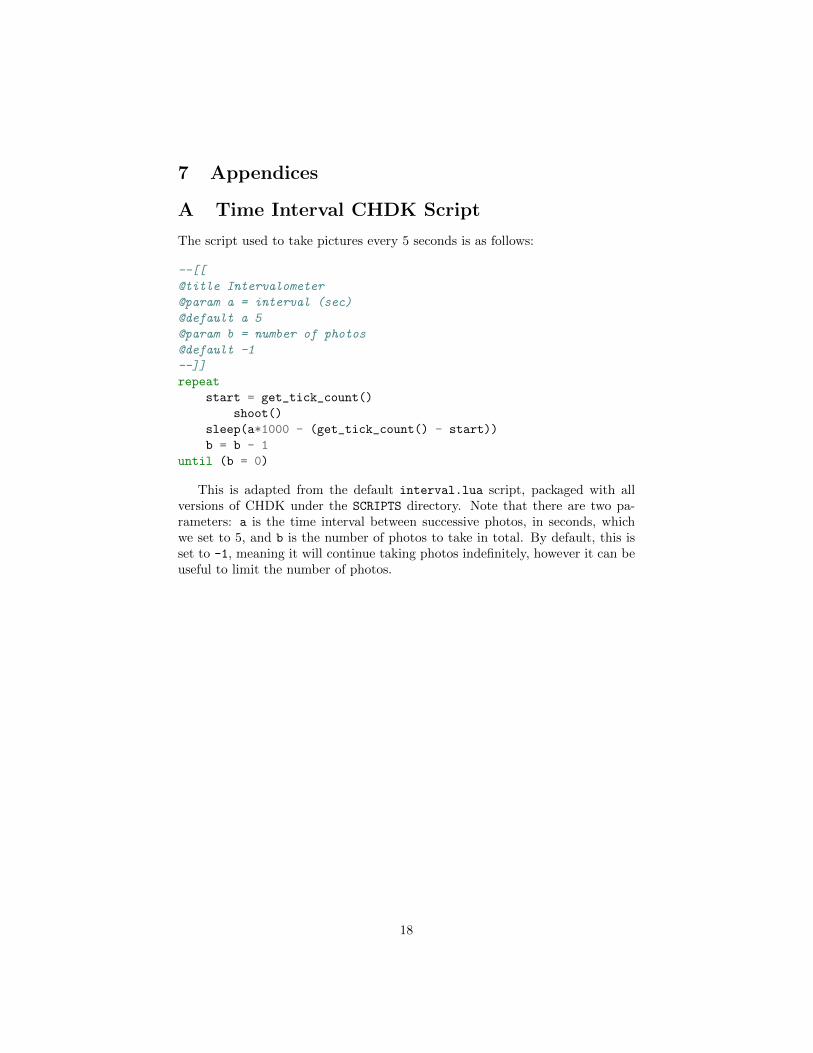
A Time Interval CHDK Script

The script used to take pictures every 5 seconds is as follows:

--[[

@title Intervalometer

@param a = interval (sec)

@default a 5

@param b = number of photos

@default -1

--]]

repeat

start = get_tick_count()

shoot()

sleep(a*1000 - (get_tick_count() - start))

b = b - 1

until (b = 0)

This is adapted from the default interval.lua script, packaged with allversions of CHDK under the SCRIPTS directory. Note that there are two pa-rameters: a is the time interval between successive photos, in seconds, whichwe set to 5, and b is the number of photos to take in total. By default, this isset to -1, meaning it will continue taking photos indefinitely, however it can beuseful to limit the number of photos.

18

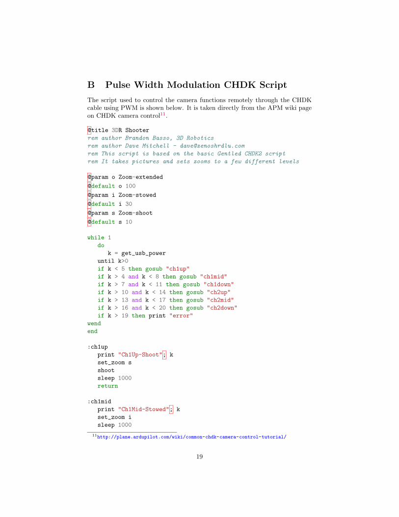
B Pulse Width Modulation CHDK Script

The script used to control the camera functions remotely through the CHDKcable using PWM is shown below. It is taken directly from the APM wiki pageon CHDK camera control11.

@title 3DR Shooter

rem author Brandon Basso, 3D Robotics

rem author Dave Mitchell - dave@zenoshrdlu.com

rem This script is based on the basic Gentled CHDK2 script

rem It takes pictures and sets zooms to a few different levels

@param o Zoom-extended

@default o 100

@param i Zoom-stowed

@default i 30

@param s Zoom-shoot

@default s 10

while 1

do

k = get_usb_power

until k>0

if k < 5 then gosub "ch1up"

if k > 4 and k < 8 then gosub "ch1mid"

if k > 7 and k < 11 then gosub "ch1down"

if k > 10 and k < 14 then gosub "ch2up"

if k > 13 and k < 17 then gosub "ch2mid"

if k > 16 and k < 20 then gosub "ch2down"

if k > 19 then print "error"

wend

end

:ch1up

print "Ch1Up-Shoot"; k

set_zoom s

shoot

sleep 1000

return

:ch1mid

print "Ch1Mid-Stowed"; k

set_zoom i

sleep 1000

11http://plane.ardupilot.com/wiki/common-chdk-camera-control-tutorial/

19

return

:ch1down

print "Ch1Down-Extended"; k

set_zoom o

sleep 1000

return

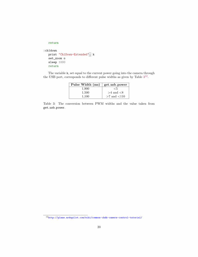
The variable k, set equal to the current power going into the camera throughthe USB port, corresponds to different pulse widths as given by Table 312.

Pulse Width (ms) get usb power1,900 <51,500 >4 and <81,100 >7 and <110

Table 3: The conversion between PWM widths and the value taken fromget usb power.

12http://plane.ardupilot.com/wiki/common-chdk-camera-control-tutorial/

20

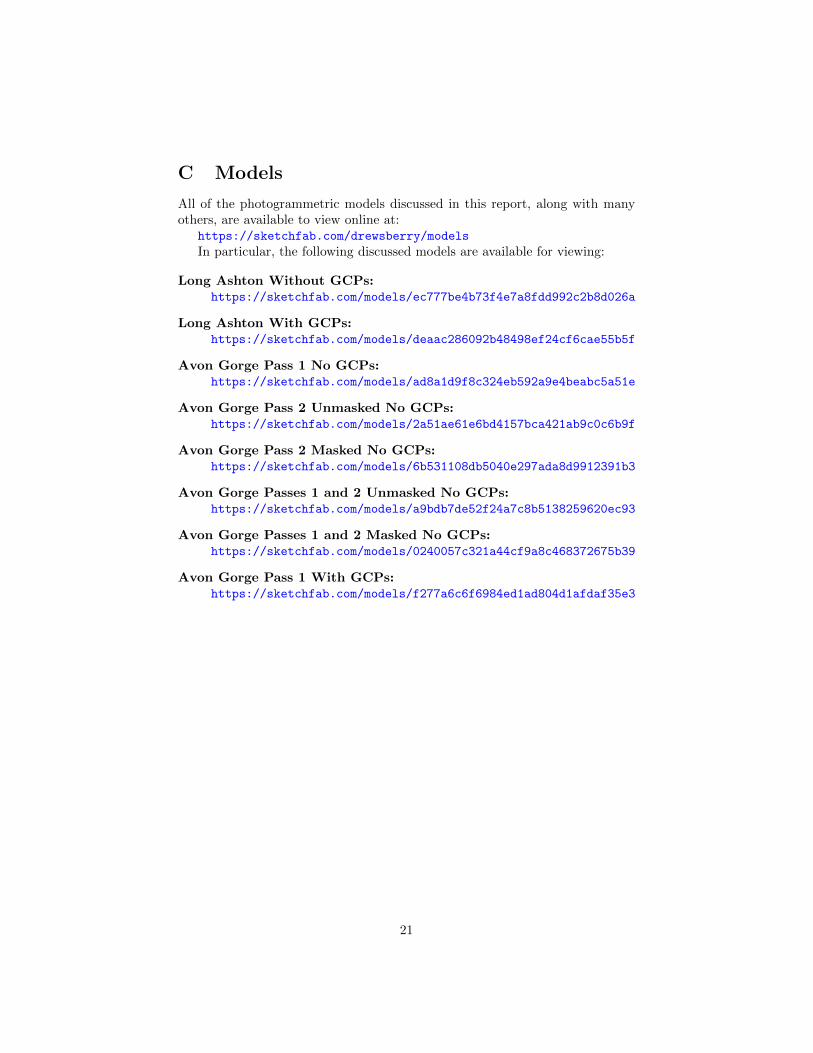
C Models

All of the photogrammetric models discussed in this report, along with manyothers, are available to view online at:

https://sketchfab.com/drewsberry/models

In particular, the following discussed models are available for viewing:

Long Ashton Without GCPs:https://sketchfab.com/models/ec777be4b73f4e7a8fdd992c2b8d026a

Long Ashton With GCPs:https://sketchfab.com/models/deaac286092b48498ef24cf6cae55b5f

Avon Gorge Pass 1 No GCPs:https://sketchfab.com/models/ad8a1d9f8c324eb592a9e4beabc5a51e

Avon Gorge Pass 2 Unmasked No GCPs:https://sketchfab.com/models/2a51ae61e6bd4157bca421ab9c0c6b9f

Avon Gorge Pass 2 Masked No GCPs:https://sketchfab.com/models/6b531108db5040e297ada8d9912391b3

Avon Gorge Passes 1 and 2 Unmasked No GCPs:https://sketchfab.com/models/a9bdb7de52f24a7c8b5138259620ec93

Avon Gorge Passes 1 and 2 Masked No GCPs:https://sketchfab.com/models/0240057c321a44cf9a8c468372675b39

Avon Gorge Pass 1 With GCPs:https://sketchfab.com/models/f277a6c6f6984ed1ad804d1afdaf35e3

21