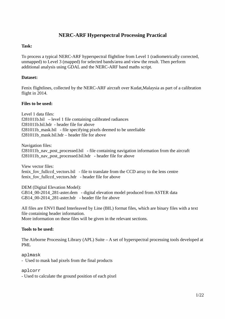
NERC-ARF Hyperspectral Processing Practical

Task:

To process a typical NERC-ARF hyperspectral flightline from Level 1 (radiometrically corrected, unmapped) to Level 3 (mapped) for selected bands/area and view the result. Then perform additional analysis using GDAL and the NERC-ARF band maths script.

Dataset:

Fenix flightlines, collected by the NERC-ARF aircraft over Kudat,Malaysia as part of a calibration flight in 2014.

Files to be used:

Level 1 data files:f281011b.bil – level 1 file containing calibrated radiances f281011b.bil.hdr - header file for abovef281011b_mask.bil - file specifying pixels deemed to be unreliablef281011b_mask.bil.hdr – header file for above

Navigation files:f281011b_nav_post_processed.bil - file containing navigation information from the aircraftf281011b_nav_post_processed.bil.hdr - header file for above

View vector files:fenix_fov_fullccd_vectors.bil - file to translate from the CCD array to the lens centrefenix_fov_fullccd_vectors.hdr - header file for above

DEM (Digital Elevation Model):GB14_00-2014_281-aster.dem - digital elevation model produced from ASTER dataGB14_00-2014_281-aster.hdr - header file for above

All files are ENVI Band Interleaved by Line (BIL) format files, which are binary files with a text file containing header information. More information on these files will be given in the relevant sections.

Tools to be used:

The Airborne Processing Library (APL) Suite – A set of hyperspectral processing tools developed atPML

aplmask- Used to mask bad pixels from the final products

aplcorr- Used to calculate the ground position of each pixel

1/22

apltran- Used to convert between different projections

aplmap- Used to create a georectified image using a level 1 file and positions calculated by aplcorr

The latest version of APL can always be downloaded from: http:// nerc-arf-dan.pml .ac.uk/trac/wiki/Downloads/software (password required – please ask)

External

GDAL

The Geospatial Data Abstraction Library (GDAL; http://www.gdal.org/index.html). Some utilities included with GDAL are used:

gdal_translate: http://www.gdal.org/gdal_translate.htmlgdalbuildvrt: http://www.gdal.org/gdalbuildvrt.htmlgdalinfo: http://www.gdal.org/gdalinfo.htmlgdaladdo: http://www.gdal.org/gdaladdo.htmlgdaladdo: http://www.gdal.org/gdaladdo.htmlgdallocationinfo: http://www.gdal.org/gdallocationinfo.html

Tuiview- An open source raster viewer based on GDAL and written in Python(http://tuiview.org/)

ARSF Scriptsget_info_from_header.py: https://github.com/pmlrsg/ arsf _toolsbandmath.py

If you are not using an NERC-ARF computer or the supplied virtual machine you will need to install these packages before starting the tutorial.

2/22

Delivery Structure

The files to be used are provided in the same structure as you will receive in your own delivery. For clarity, files not used in this demo have been removed.

This structure is detailed below:. |-- dem - Digital Elevation Model|-- doc - Documents such as the data quality report|-- flightlines

| |-- level1b - Level 1 data and mask files| |-- line_information - Metadata for each flightline| |-- mapped - Mapped level 3 files| `-- navigation - Post-processed plane navigation data|-- logsheet - Logsheet for the flight detailing all flightlines|-- project_information - Metadata for the project|-- screenshots - JPG images, giving a quicklook for each mapped flightline`-- sensor_FOV_vectors - CCD pixel view vectors

The only relevant directories for this task are dem, flightlines/level1b, flightlines/navigation and sensor_FOV_vectors.

Further information on directory structures will be provided in the ReadMe for you project. An up-to-date layout description is also located at:http s :// nerc-arf- dan . pml .nerc.ac.uk/trac/wiki/Processing/FilenameConventions#Delivereddata

Procedure

Instructions will be given both for the APL GUI (Graphical User Interface) and command line. If you are already familiar with the command line you can skip the GUI section. An advantage of learning the command line over the GUI is it makes it easier for batch processing, i.e., applying the same process to multiple flight lines.

Windows vs Linux

Some people will be performing this demo on a Windows machine, and others on Linux. All of the software and examples have been tested on both operating systems. Windows traditionally uses backslashes to separate paths (e.g. ...\dir\subdir\file) and Linux uses forward slashes (e.g. .../dir/subdir/file). The latter convention has been used in the examples, however you should be ableto copy the example commands straight into both as modern Windows versions can handle both types. Where commands span multiple lines in the worksheet '\' has been used, for Windows you will need to use '^' instead or just paste one line at a time.

If you are using an NERC-ARF computer or the virtual machine the data to be used is located at:

~/nerc-arf-workshop/hyperspectral_practical

3/22

Before starting you need to open a terminal window (Applications → Terminal) and navigate to the directory the data are stored by typing:

cd ~/nerc-arf-workshop/hyperspectral_practical

Then pressing enter.

On Windows if you created a 'start_apl.bat' file when you installed APL (see earlier instructions) click on this to open a command prompt. If not open open a command prompt and type :

set PATH=”C:\APL”;%PATH%

Substituting “C\APL” to where you downloaded and extracted the APL binaries to.

Next, navigate to the data directory by typing:

cd C:\nerc-arf-workshop\hyperspectral_practical\

Changing the path to where the data are stored.

Within the practical directory create a folder to store outputs called 'outputs'. You can do this from within a terminal window / command prompt using the following command:

mkdir outputs

4/22

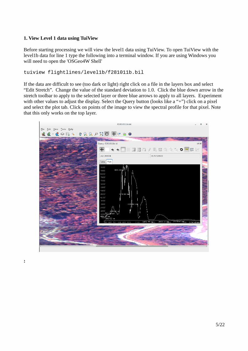
1. View Level 1 data using TuiView

Before starting processing we will view the level1 data using TuiView. To open TuiView with the level1b data for line 1 type the following into a terminal window. If you are using Windows you will need to open the 'OSGeo4W Shell'

tuiview flightlines/level1b/f281011b.bil

If the data are difficult to see (too dark or light) right click on a file in the layers box and select “Edit Stretch”. Change the value of the standard deviation to 1.0. Click the blue down arrow in thestretch toolbar to apply to the selected layer or three blue arrows to apply to all layers. Experiment with other values to adjust the display. Select the Query button (looks like a “+”) click on a pixel and select the plot tab. Click on points of the image to view the spectral profile for that pixel. Note that this only works on the top layer.

:

5/22

2. Masking bad pixels with aplmask

The first step is to apply the mask of bad pixels to the level 1 file, creating a new level 1 file with these pixels set to 0. Pixels can be 'bad' for many reasons (see mask section below).

The level 1 file

The level 1b file has had a radiometric calibration applied to give actual radiance values as seen by the sensor. It has not been adjusted for atmospheric interference and it has not been georectified in any way, so appears as a straight rectangle of collected data. It is a binary file, meaning only specialised programs can view it. The “.bil” part of the name refers to the way the bands/channels are stored within the file, in this instance Band Interleaved by Line.

The mask file

This is a BIL file of the same dimensions as the raw file. For every single pixel in the image (for all bands), a value is given which is the summation of the below flags:

0 = Good data.1 = Underflows.2 = Overflows.4 = Bad CCD pixels.8 = Pixel affected by uncorrected smear.16 = Dropped scans.32 = Corrupt raw data.64 = Quality control failures.

A single pixel can have multiple flags. This file was created at an earlier stage in the processing chain (namely by aplcal) when various algorithms are used to identify pixels as one of the above.

Header files

Although not always explicitly mentioned in this tutorial, every time you create a new .bil file, a matching .bil.hdr file will be created. This is required as it tells programs how to interpret the BIL file. You can examine this file in any text editor and will give you useful information such as the number of bands and the width and length of the flightline.

GUI

To open the APL GUI go to a terminal Window and type:

aplgui &

6/22

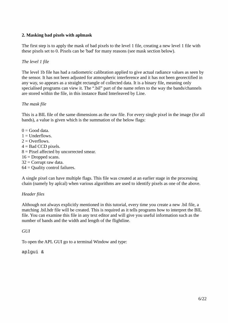
The following window will appear:

1. First off if you are not using an NERC-ARF workstation or the VM you'll need to point it at the APL executable directory so it can find the underpinning APL programs on which it is based. Click File → Executable Path and point it at /usr/local/bin / C:\APL (or wherever youhave saved the APL files).

2. Next we'll give it the main directory of our dataset, to make finding our input files easier in the next steps.

3. Click File → Project Directory and point it at nerc-arf-workshop/hyperspectral_practical

4. Finally, click File → Output directory and point it at your desired output location.

5. The above steps mean that future clicks of the Browse button should take you automatically to the correct directory.

6. Click Browse and find the level 1 file: flightlines/level1b/f281011b.bil and the mask file: flightlines/level1b/f281011b_mask.bil

7. Click 'Save As' for the output file and save as outputs/f281011b_masked.bil

8. You can specify which mask flags to remove from the output image by ticking the appropriate boxes. Leave all of them ticked to filter out all problem pixels.

7/22

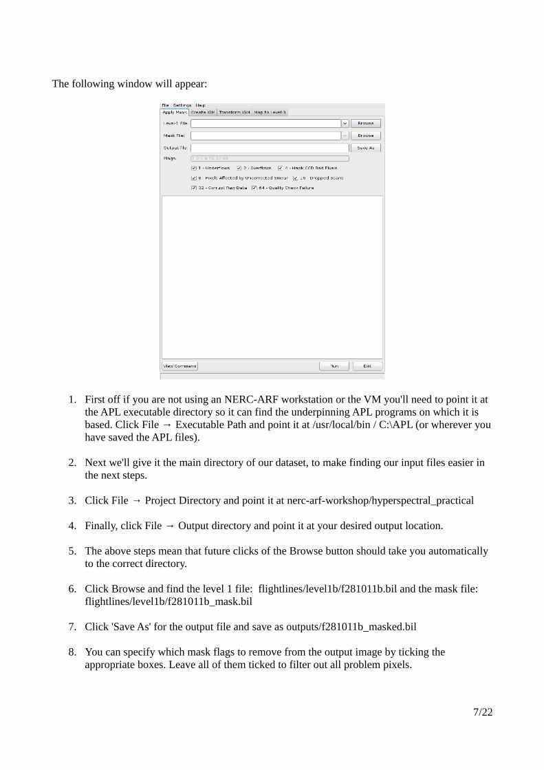
9. Click 'View Command' this shows the command which APL will run. Press 'Copy to Clipboard', we will use this to run from the command line later.

10. Click Run.

11. You should have something looking like the image below. Check for any error messages in the output.

Command Line

The command line instructions are all typed into a terminal window / command prompt. You can use the same window as the one used to start APL, if you are on Linux you might need to press enter to get to a new line.

The first command to run is:

aplmask -lev1 flightlines/level1b/f281011b.bil \ -mask flightlines/level1b/f281011b_mask.bil \ -output outputs/f281011b_masked.bil

8/22

Command break down:

-lev1: The input level 1 file-mask: The mask file to be used-output: The output level 1 file, with the mask appliedThis is the same command run within the APL GUI. Therefore, you can just paste this by right clicking within the terminal window and selecting paste. Note – the command pasted from the APL GUI will be slightly different, it will have all the flags specified, this is the default so the command can be shortened by not including it (if you have to type it out). The full path to each file is also used.

Go to a new line (by pressing Enter) to run the command.

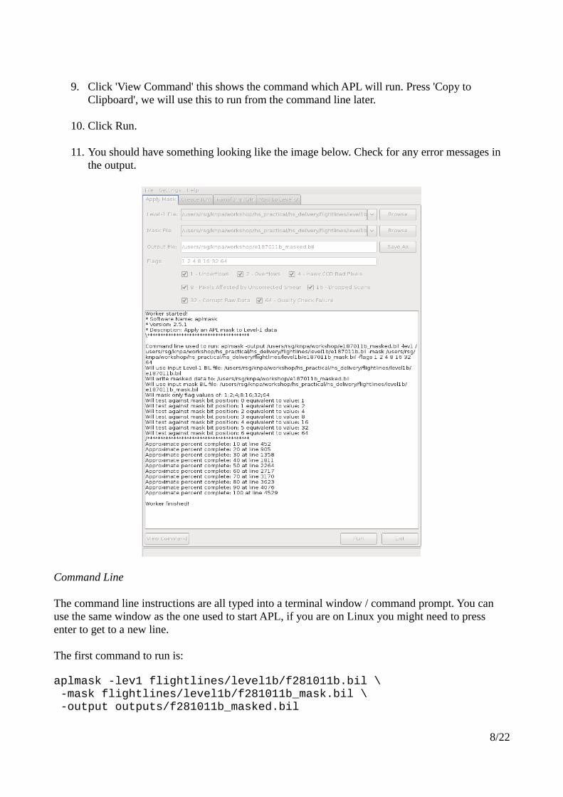
Compare the masked files to the origional by viewing in TuiView. Type:

tuiview --separate flightlines/level1b/f281011b.bil \ outputs/f281011b_masked.bil

Use the query button on both TuiView windows to compare spectra in the original and masked files.

9/22

3. Generate an IGM with aplcorr

The next step uses the navigation file, the view vector file and the digital elevation file (DEM) to work out the real world ground position for each pixel in the level 1 file.

The IGM file

The Input GeoMetry file is a two dimensional binary image designed to hold the geographical position of each pixel in the level 1 file.

The navigation file

This is a binary BIL file which contains position and attitude information for the plane for the duration of the flightline. The file's “bands” in this case are 7 variables: time, latitude, longitude, height, pitch, roll and heading. There is a separate file for each instrument, due to the instruments differing position and orientation within the aircraft. This file was generated earlier using another tool in the APL suite, aplnav.

The view vector/field of view file

This file should not change within the lifetime of the sensor and is simply a way to translate from the CCD array to the principal point of the lens and hence to the correct position on the ground. Beyond remembering to include it, you do not need to worry about this file.

The DEM file

The Digital Elevation Model is a binary file for which each pixel has a value corresponding to it's height above a given reference. Our DEM is measured against the WGS84 ellipsoid and has a pixel size of 30m. It has been produced from data from the satellite based ASTER sensor, through a collaboration between Japan and NASA (http://www.jspacesystems.or.jp/ersdac/GDEM/E/).It is perfectly possible to process your data without a DEM, however where the terrain varies significantly, this will result in positioning errors.

GUI

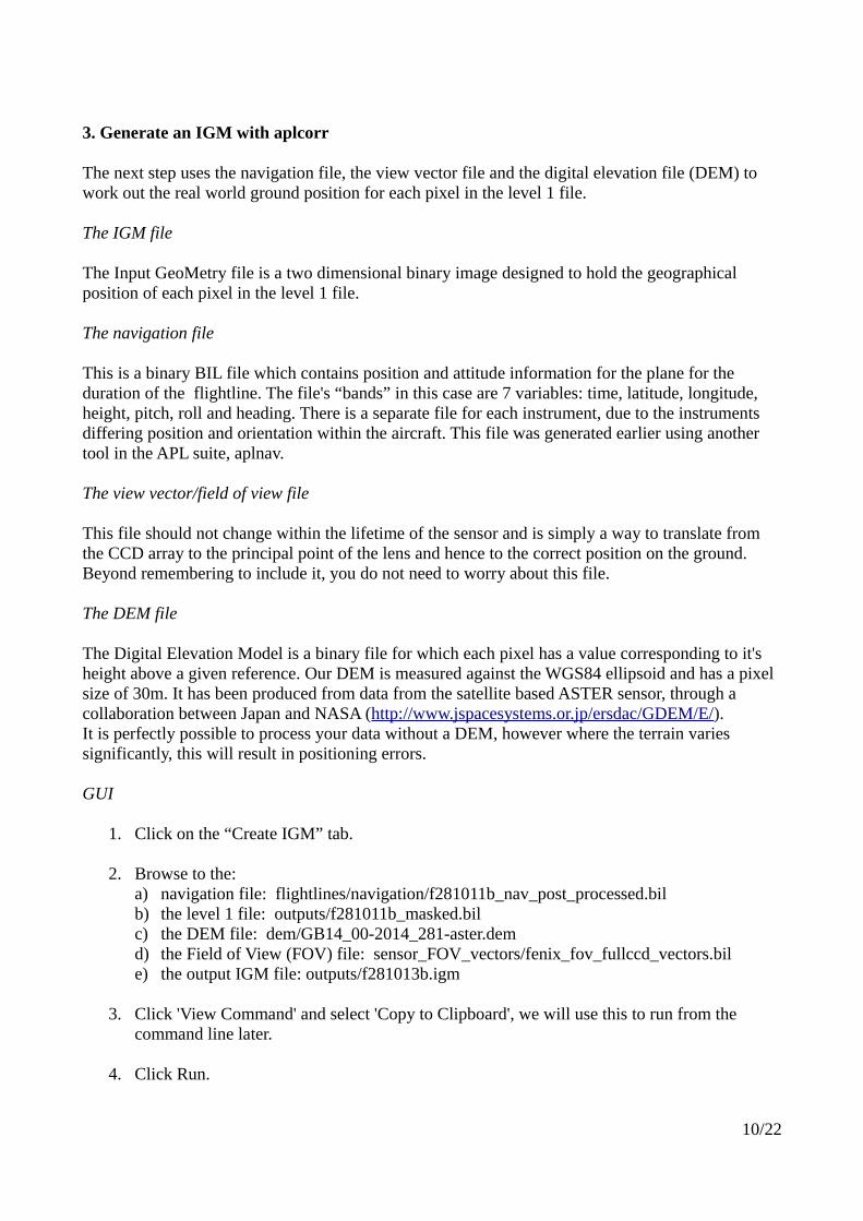
1. Click on the “Create IGM” tab.

2. Browse to the:a) navigation file: flightlines/navigation/f281011b_nav_post_processed.bilb) the level 1 file: outputs/f281011b_masked.bil c) the DEM file: dem/GB14_00-2014_281-aster.demd) the Field of View (FOV) file: sensor_FOV_vectors/fenix_fov_fullccd_vectors.bile) the output IGM file: outputs/f281013b.igm

3. Click 'View Command' and select 'Copy to Clipboard', we will use this to run from the command line later.

4. Click Run.

10/22

5. Check output for errors.

Command Line

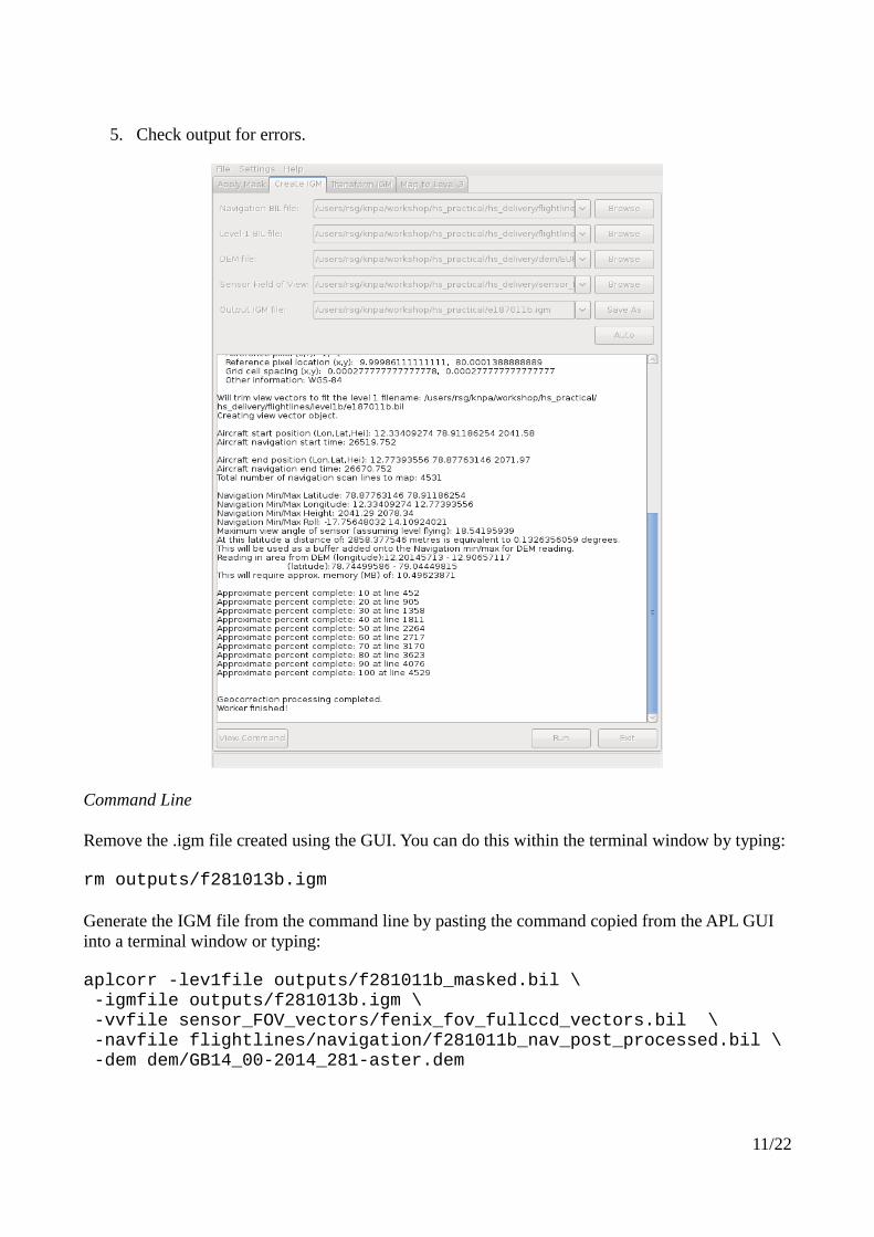
Remove the .igm file created using the GUI. You can do this within the terminal window by typing:

rm outputs/f281013b.igm

Generate the IGM file from the command line by pasting the command copied from the APL GUI into a terminal window or typing:

aplcorr -lev1file outputs/f281011b_masked.bil \ -igmfile outputs/f281013b.igm \ -vvfile sensor_FOV_vectors/fenix_fov_fullccd_vectors.bil \ -navfile flightlines/navigation/f281011b_nav_post_processed.bil \ -dem dem/GB14_00-2014_281-aster.dem

11/22

Command break down:

-lev1file: The input level 1 file (can be the masked or original, doesn't matter for this stage)-igmfile: The output IGM file-vvfile: The sensor's view vector /field of view file-navfile: The navigation file for the flightline-dem: The Digital Elevation Model

4. Change the projection of the IGM with apltran

The IGM output by aplcorr is always in latitude-longitude, so if you want to change the projection, for instance to match another dataset, then you should use apltran. We will be changing the projection from lat-long to UTM (Universal Transverse Mercator) to match the LiDAR data NERC-ARF also acquire.

UK command

The below instructions are for changing from lat-long to UTM. If your project is in the UK then in the apltran command substitute `utm_wgs84N <UTM zone>` for `osng <gridfile>` where gridfile isa file describing the transform from lat-long to British National Grid. The file is called OSTN02_NTv2.gsb and can be downloaded freely from the OS website:http://www.ordnancesurvey.co.uk/oswebsite/support/os-net/ostn02-ntv2-format.html

If using the GUI then select the “OSGB36 NB” radio button and browse to the downloaded gridfile.

GUI

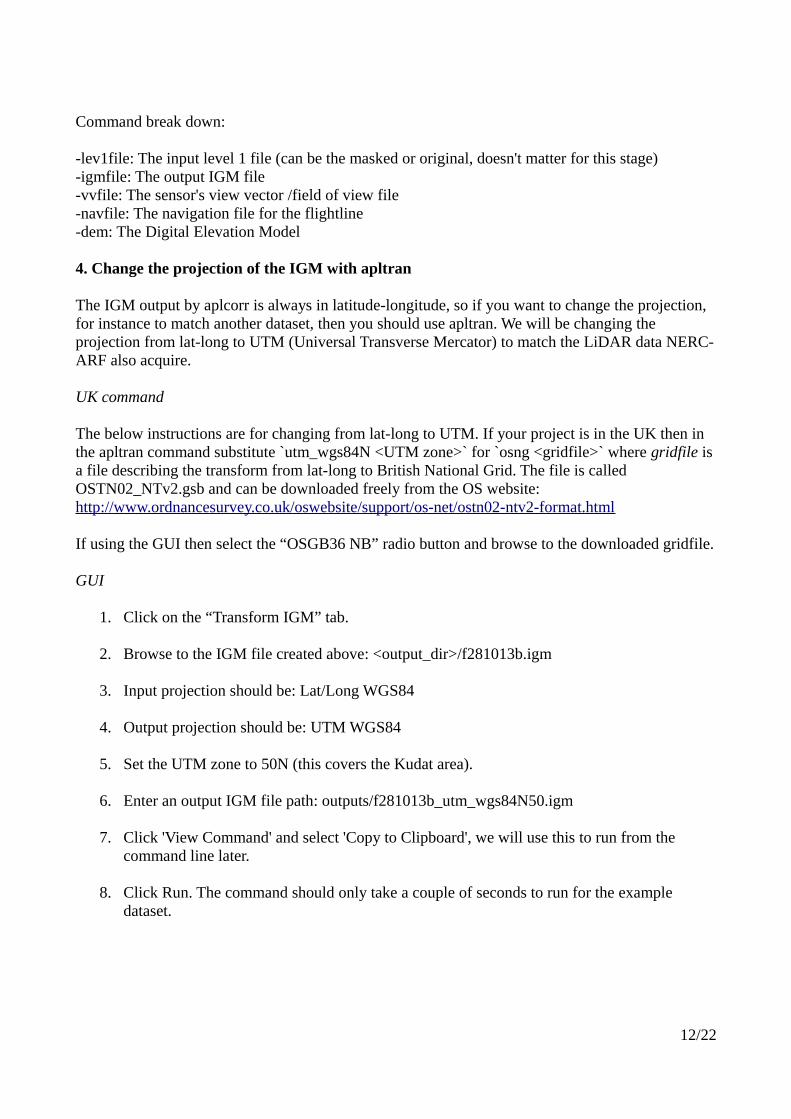
1. Click on the “Transform IGM” tab.

2. Browse to the IGM file created above: <output_dir>/f281013b.igm

3. Input projection should be: Lat/Long WGS84

4. Output projection should be: UTM WGS84

5. Set the UTM zone to 50N (this covers the Kudat area).

6. Enter an output IGM file path: outputs/f281013b_utm_wgs84N50.igm

7. Click 'View Command' and select 'Copy to Clipboard', we will use this to run from the command line later.

8. Click Run. The command should only take a couple of seconds to run for the example dataset.

12/22

Command Line

Remove the .igm file created using the GUI. You can do this within the terminal window by typing:

rm outputs/f281013b_utm_wgs84N50.igm

If you copied the command from the APL GUI paste into the terminal window and press enter to run. Otherwise enter the following:

apltran -inproj latlong WGS84 \ -igm outputs/f281013b.igm \ -output outputs/f281013b_utm_wgs84N50.igm \ -outproj utm_wgs84N 50

Command break down:

-inproj: Input projection (we've specified lat-long, which is the default)-igm: Your input igm file created by aplcorr, in lat-long

13/22

-output: Your output igm file (which will be in osng)-outproj: The output projection – if UTM be sure to give the correct UTM zone (50 covers Kudat)

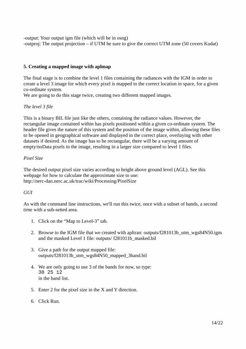
5. Creating a mapped image with aplmap

The final stage is to combine the level 1 files containing the radiances with the IGM in order to create a level 3 image for which every pixel is mapped to the correct location in space, for a given co-ordinate system.We are going to do this stage twice, creating two different mapped images.

The level 3 file

This is a binary BIL file just like the others, containing the radiance values. However, the rectangular image contained within has pixels positioned within a given co-ordinate system. The header file gives the nature of this system and the position of the image within, allowing these files to be opened in geographical software and displayed in the correct place, overlaying with other datasets if desired. As the image has to be rectangular, there will be a varying amount of empty/noData pixels in the image, resulting in a larger size compared to level 1 files.

Pixel Size

The desired output pixel size varies according to height above ground level (AGL). See this webpage for how to calculate the approximate size to use: http://nerc-dan.nerc.ac.uk/trac/wiki/Processing/PixelSize

GUI

As with the command line instructions, we'll run this twice, once with a subset of bands, a second time with a sub-setted area.

1. Click on the “Map to Level-3” tab.

2. Browse to the IGM file that we created with apltran: outputs/f281013b_utm_wgs84N50.igmand the masked Level 1 file: outputs/ f281011b_masked.bil

3. Give a path for the output mapped file: outputs/f281013b_utm_wgs84N50_mapped_3band.bil

4. We are only going to use 3 of the bands for now, so type:38 25 12in the band list.

5. Enter 2 for the pixel size in the X and Y direction.

6. Click Run.

14/22

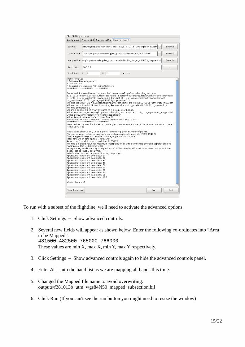
To run with a subset of the flightline, we'll need to activate the advanced options.

1. Click Settings → Show advanced controls.

2. Several new fields will appear as shown below. Enter the following co-ordinates into “Area to be Mapped”:481500 482500 765000 766000These values are min X, max X, min Y, max Y respectively.

3. Click Settings → Show advanced controls again to hide the advanced controls panel.

4. Enter ALL into the band list as we are mapping all bands this time.

5. Changed the Mapped file name to avoid overwriting: outputs/f281013b_utm_wgs84N50_mapped_subsection.bil

6. Click Run (If you can't see the run button you might need to resize the window)

15/22

Command Line

First we'll map the whole flightline, using three selected bands. You can view the list of bands and their wavelengths in the header files.

Command:

aplmap -igm outputs/f281013b_utm_wgs84N50.igm \ -lev1 outputs/f281011b_masked.bil \ -mapname outputs/f281013b_utm_wgs84N50_mapped_3band.bil \ -pixelsize 2 2 \ -bandlist 38 25 12

Command Break Down:

-igm: The transformed IGM created in the above step-lev1: The masked BIL file created by aplmask in step 1-mapname: The output georectified BIL image-pixelsize: Output pixel size, in metres, in the x and y direction-bandlist: A space separated list of bands to be placed in the output image

Next, we'll map a spatial subset of the flightline, using all bands.

Command:

aplmap -igm outputs/f281013b_utm_wgs84N50.igm \ -lev1 outputs/f281011b_masked.bil \ -mapname outputs/f281013b_utm_wgs84N50_mapped_subsection.bil \ -pixelsize 2 2 \ -bandlist ALL \ -area 481500 482500 765000 766000

Command Break Down:

-area: A rectangular region specifying the area to process in the order min X, max X, min Y, max Y. We are using UTM coordinates so these are in meters, the X value measured from the edge of the UTM zone and the Y value from the equator.

To extract a chosen area or bands from the already mapped image, we recommend using gdal_translate.

16/22

6. Running all the commands together for a second line

Running each step individually requires a lot of manual intervention – for processing a lot of flight lines a better option is to create a script which can run all the commands one after the other. The simplest version of a script is a text file containing a list of commands to be run. For R users, it is possible to run from within an R script by using the system function to call each APL command. See run_apl.r for an example. If you are not familiar with R proceed with the following steps:

1. Create a script with all the commands to be run. If you are using Linux type:

gedit run_all_apl_commands_file2.sh

into the terminal window. This will create a new file and open it for editing in gedit.If you are using Windows type:

notepad run_all_apl_commands_file2.sh

Paste the following text into the editor:

aplmask -lev1 flightlines/level1b/f281021b.bil \ -mask flightlines/level1b/f281021b_mask.bil \ -output outputs/f281021b_masked.bil

aplcorr -lev1file outputs/f281021b_masked.bil \ -igmfile outputs/f281023b.igm \ -vvfile sensor_FOV_vectors/fenix_fov_fullccd_vectors.bil \ -navfile \ flightlines/navigation/f281021b_nav_post_processed.bil \ -dem dem/GB14_00-2014_281-aster.dem

apltran -inproj latlong WGS84 \ -igm outputs/f281023b.igm \ -output outputs/f281023b_utm_wgs84N50.igm \ -outproj utm_wgs84N 50

aplmap -igm outputs/f281023b_utm_wgs84N50.igm \ -lev1 outputs/f281021b_masked.bil \ -mapname outputs/f281023b_utm_wgs84N50_mapped_3band.bil \ -pixelsize 2 2 -bandlist 38 25 12

Remembering to change from '\' to '^' if you are using Windows.

2. Save the file and close gedit / notepad.

17/22

3. Run the script using the following command (tip – if you start typing the name you can use tab to complete). For Linux:

sh run_all_apl_commands_file2.sh

For Windows

run_all_apl_commands_file2

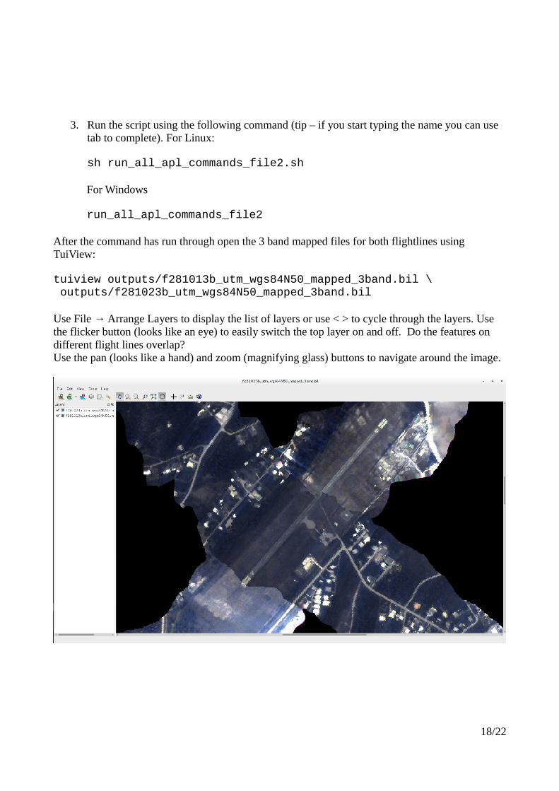
After the command has run through open the 3 band mapped files for both flightlines using TuiView:

tuiview outputs/f281013b_utm_wgs84N50_mapped_3band.bil \ outputs/f281023b_utm_wgs84N50_mapped_3band.bil

Use File → Arrange Layers to display the list of layers or use < > to cycle through the layers. Use the flicker button (looks like an eye) to easily switch the top layer on and off. Do the features on different flight lines overlap?Use the pan (looks like a hand) and zoom (magnifying glass) buttons to navigate around the image.

18/22

7. Additional Analysis using GDAL

Unlike the subset area or band images you have created above, the level 3 mapped images supplied in an NERC-ARF delivery are of the whole flightline and for all bands. Once unzipped, these files can run into hundreds of gigabytes (so for space reasons, an example file has not been included in the practical).

a) Create subset and change format

Command:

gdal_translate -of GTiff -co COMPRESS=LZW \ -projwin 481500 766000 482500 765000 \ -b 190 -b 40 -b 15 \ outputs/f281013b_utm_wgs84N50_mapped_subsection.bil \ outputs/f281013b_utm_wgs84N50_mapped_subsection_3band.tif

Command break down:

-of: Output Format - we are using GeoTiff file. For all available options see http://www.gdal.org/formats_list.html-co: Creation Option – specifies the creation options, these are specific to the format. For GeoTiff we use compression to reduce the file size. For ENVI we can use the creation options to specify the Interleave (BSQ or BIL)-projwin: A rectangle delineating an area to be extracted, in the format min X min Y max X max Y-b: A given band to extractfinal two arguments: input and output filenames

b) Create mosaic of multiple flightlines

Often a mosaic of all individual flightlines is required. Due to the large sizes of the mapped files this can often be time consuming. One option is to first make a 'Virtial Raster' using the 'gdalbuildvrt' command:

gdalbuildvrt -srcnodata 0 outputs/f2810_mapped_mosaic.vrt \ outputs/f281013b_utm_wgs84N50_mapped_3band.bil \ outputs/f281023b_utm_wgs84N50_mapped_3band.bil

Command break down:

-srcnodata: No data value of input linesfirst argument: output VRT filefinal arguments: list of input files

Rather than creating a new file a small .vrt text file is created which contains links to the individual lines.

19/22

Many programs which use GDAL (e.g., TuiView) can open this file directly. To make opening the file easier we can do some optimisation. First pre-calculate statistics using:

gdalinfo -stats outputs/f2810_mapped_mosaic.vrt

Command break down:

-stats: Calculate statistics and save to .aux.xml filefinal argument: file name

The gdalinfo command can also be used to print information about a raster. Note for the .vrt file it shows the individual files which are included.

After creating statistics generate overviews (lower resolution copies at different resolutions) using gdaladdo:

gdaladdo -r average outputs/f2810_mapped_mosaic.vrt 2 4 8 16

Command break down:

-r average: Use average for resampling overviewsfirst argument: file namenumbers: overview levels to build (2x, 4x, 8x and 16x)

Finally open in TuiView using

tuiview outputs/f2810_mapped_mosaic.vrt

We can also make a real raster using gdal_translate (as shown previously).

c) Extract pixel values for a given location

gdallocationinfo -valonly -geoloc \ outputs/f281013b_utm_wgs84N50_mapped_subsection.bil \ 481801 765289

Command break down:

-valonly: Only print values to the screen-geoloc: Interprerate x and y values as coordinates rather than pixel and linefirst argument: file namex y: Easting and Northing of pixel to extract statistics from

This will print the values to the screen. To save as a text file we can redirect the output using '>'

gdallocationinfo -valonly -geoloc \ outputs/f281013b_utm_wgs84N50_mapped_subsection.bil \ 481801 765289 > outputs/extracted_values.txt

20/22

This text file can be opened in other programs for further analysis.8. Calculate NDVI

The Normalised Difference Vegetation Index (NDVI) is a commonly used index of vegetation productivity and is a ratio of NIR and Red bands.

NDVI = (NIR-Red) / (NIR+Red)

For this example we will use 800 nm for the NIR channel and 670 nm for the Red channel.

a) Get wavelengths

The first step is to extract the wavelengths from the header file to a .csv file, which can be opened inExcel / LibreOffice. For this the 'get_info_from_header.py' script from NERC-ARF is used:

get_info_from_header.py \ -o outputs/f281011b_masked_wavelengths.csv \ outputs/f281011b_masked.bil.hdr

Click to open this file in Excel / LibreOffice or type:

oocalc outputs/f281011b_masked_wavelengths.csv &

Find the bands corresponding to these approximately these wavelengths.

b) Calculate NDVI

The next step is to use the bandmath.py command to calculate NDVI for each pixel within a hyperspectral file:

bandmath.py \ --equation "(band246 - band171) / (band246 + band171)" \ --ename NDVI \ --output_folder outputs \ outputs/f281011b_masked.bil

Command break down:--equation: equation to calculate, bands provided in the format band000--ename: equation name to use for file, if not provided will use equation--output_folder: folder to save output tofinal argument: input .bil file

View using:

tuiview outputs/f281011b_masked_NDVI.bil

Note, some there are some gaps due to bad pixels being masked out.

21/22

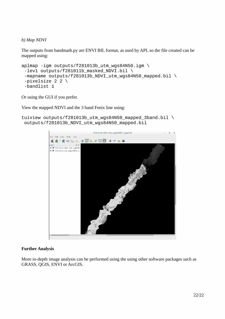
b) Map NDVI

The outputs from bandmath.py are ENVI BIL format, as used by APL so the file created can be mapped using:

aplmap -igm outputs/f281013b_utm_wgs84N50.igm \ -lev1 outputs/f281011b_masked_NDVI.bil \ -mapname outputs/f281013b_NDVI_utm_wgs84N50_mapped.bil \ -pixelsize 2 2 \ -bandlist 1

Or using the GUI if you prefer.

View the mapped NDVI and the 3 band Fenix line using:

tuiview outputs/f281013b_utm_wgs84N50_mapped_3band.bil \ outputs/f281013b_NDVI_utm_wgs84N50_mapped.bil

Further Analysis

More in-depth image analysis can be performed using the using other software packages such as GRASS, QGIS, ENVI or ArcGIS.

22/22