Embed Size (px)
Citation preview
NeMo user manual
Andreas K. FidjelandPedro A.M. Mediano 〈[email protected]〉
July 22, 2016 Version 0.7.2
Abstract
NeMo is a library for discrete-time simulation of spiking neural networks.It is aimed at real-time simulation of tens of thousands of neurons on asingle workstation. NeMo runs on parallel hardware; in particular it canrun on CUDA-enabled GPUs. No parallel programming is required onthe part of the end user, as parallelisation is handled by the library. Thelibrary has interfaces in C++, C, Python, and Matlab.
1 A short tutorial introduction
The NeMo library can be used to simulate a network of point neurons. Thelibrary can support different types neuron models via a plugin system. Thecurrent version of the library ships with support for Izhikevich neurons [5] andKuramoto oscillators [6].
The library exposes three basic types of objects: network, configuration, andsimulation. Setting up and running such a simulation involves:
1. Creating a network object and adding neurons and synapses;
2. Creating a configuration object and setting its parameters; and
3. Creating a simulation object from the network and configuration objectsand running the simulation.
The following section illustrates basic usage of the library using the Pythoninterface. The other language interfaces (Section 3) have similar usage.
1.1 Constructing a network
Network construction is performed using a low-level interface where neuronsand synapses are added individually. The Python and Matlab APIs have vector
1
forms for some functions, but fundamentally each neuron and synapse must beindividually specified. Higher-level construction interfaces, e.g. using variousforms of projections, can be built on top of this, but is not part of NeMo. Onesuch system is BrainStudio, also built and maintained by part of the NeMo team.
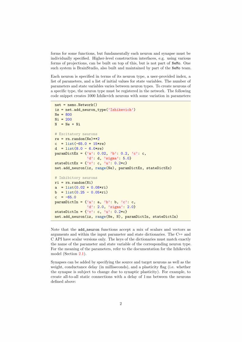
Each neuron is specified in terms of its neuron type, a user-provided index, alist of parameters, and a list of initial values for state variables. The number ofparameters and state variables varies between neuron types. To create neurons ofa specific type, the neuron type must be registered in the network. The followingcode snippet creates 1000 Izhikevich neurons with some variation in parameters:
net = nemo.Network()
iz = net.add_neuron_type(’Izhikevich’)
Ne = 800
Ni = 200
N = Ne + Ni
# Excitatory neurons
re = rn.random(Ne)**2
c = list(-65.0 + 15*re)
d = list(8.0 - 6.0*re)
paramDictEx = {’a’: 0.02, ’b’: 0.2, ’c’: c,
’d’: d, ’sigma’: 5.0}
stateDictEx = {’v’: c, ’u’: 0.2*c}
net.add_neuron(iz, range(Ne), paramDictEx, stateDictEx)
# Inhibitory neurons
ri = rn.random(Ni)
a = list(0.02 + 0.08*ri)
b = list(0.25 - 0.05*ri)
c = -65.0
paramDictIn = {’a’: a, ’b’: b, ’c’: c,
’d’: 2.0, ’sigma’: 2.0}
stateDictIn = {’v’: c, ’u’: 0.2*c}
net.add_neuron(iz, range(Ne, N), paramDictIn, stateDictIn)
Note that the add_neuron functions accept a mix of scalars and vectors asarguments and within the input parameter and state dictionaries. The C++ andC API have scalar versions only. The keys of the dictionaries must match exactlythe name of the parameter and state variable of the corresponding neuron type.For the meaning of the parameters, refer to the documentation for the Izhikevichmodel (Section 2.1).
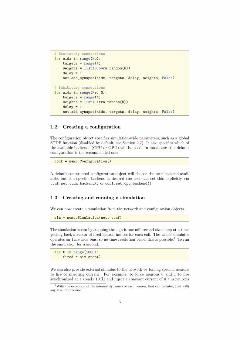
Synapses can be added by specifying the source and target neurons as well as theweight, conductance delay (in milliseconds), and a plasticity flag (i.e. whetherthe synapse is subject to change due to synaptic plasticity). For example, tocreate all-to-all static connections with a delay of 1 ms between the neuronsdefined above:
2
# Excitatory connections
for nidx in range(Ne):
targets = range(N)
weights = list(0.5*rn.random(N))
delay = 1
net.add_synapse(nidx, targets, delay, weights, False)
# Inhibitory connections
for nidx in range(Ne, N):
targets = range(N)
weights = list(-1*rn.random(N))
delay = 1
net.add_synapse(nidx, targets, delay, weights, False)
1.2 Creating a configuration
The configuration object specifies simulation-wide parameters, such as a globalSTDP function (disabled by default, see Section 2.7). It also specifies which ofthe available backends (CPU or GPU) will be used. In most cases the defaultconfiguration is the recommended one:
conf = nemo.Configuration()
A default-constructed configuration object will choose the best backend avail-able, but if a specific backend is desired the user can set this explicitly viaconf.set_cuda_backend() or conf.set_cpu_backend().
1.3 Creating and running a simulation
We can now create a simulation from the network and configuration objects.
sim = nemo.Simulation(net, conf)
The simulation is run by stepping through it one millisecond-sized step at a time,getting back a vector of fired neuron indices for each call. The whole simulatoroperates on 1 ms-wide bins, so no time resolution below this is possible.1 To runthe simulation for a second:
for t in range(1000):
fired = sim.step()
We can also provide external stimulus to the network by forcing specific neuronsto fire or injecting current. For example, to force neurons 0 and 1 to firesynchronized at a steady 10 Hz and inject a constant current of 0.7 in neurons
1With the exception of the internal dynamics of each neuron, that can be integrated withany level of precision
3
2 and 3 for 10 s one could do the following (ignoring firing output for the timebeing):
stimulus = [0, 1]
current = [(2, 0.7), (3, 0.7)]
for t in range(10000):
if t % 100 == 0:
sim.step(fstim=stimulus, istim=current)
else:
sim.step(istim=current)
The collection of examples above shows the basic usage of the simulator. The usercan perform other actions on the simulation object as well including queryingneuron or synapse data, and activate STDP (Section 2.7).
For full details of library usage refer to the language-specific notes (Section 3)and the online language-specific function reference.
2 Simulation model
NeMo has a plugin system which can support different types of neurons. Thisversion ships with support for Izhikevich neurons (Section 2.1), Poisson spikesources (Section 2.3), ancillary input neurons (Section 2.4), and both delay- andphase-coupled Kuramoto oscillators (Section 2.5).
2.1 Izhikevich neurons
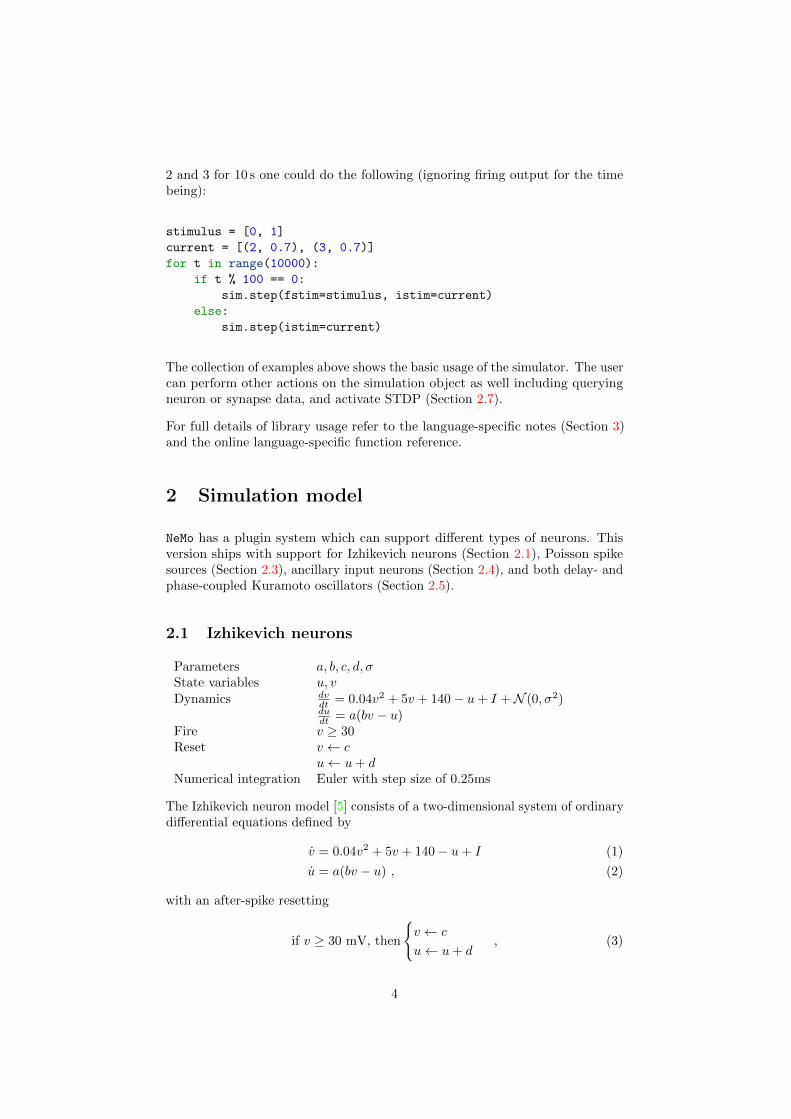
Parameters a, b, c, d, σState variables u, vDynamics dv
dt = 0.04v2 + 5v + 140− u+ I +N (0, σ2)dudt = a(bv − u)
Fire v ≥ 30Reset v ← c
u← u+ dNumerical integration Euler with step size of 0.25ms
The Izhikevich neuron model [5] consists of a two-dimensional system of ordinarydifferential equations defined by
v = 0.04v2 + 5v + 140− u+ I (1)
u = a(bv − u) , (2)
with an after-spike resetting
if v ≥ 30 mV, then
{v ← c
u← u+ d, (3)
4
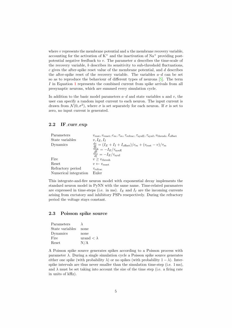
where v represents the membrane potential and u the membrane recovery variable,accounting for the activation of K+ and the inactivation of Na+ providing post-potential negative feedback to v. The parameter a describes the time-scale ofthe recovery variable, b describes its sensitivity to sub-threshold fluctuations,c gives the after-spike reset value of the membrane potential, and d describesthe after-spike reset of the recovery variable. The variables a–d can be setso as to reproduce the behaviour of different types of neurons [5]. The termI in Equation 1 represents the combined current from spike arrivals from allpresynaptic neurons, which are summed every simulation cycle.
In addition to the basic model parameters a–d and state variables u and v, theuser can specify a random input current to each neuron. The input current isdrawn from N (0, σ2), where σ is set separately for each neuron. If σ is set tozero, no input current is generated.
2.2 IF curr exp
Parameters vrest, vreset, cm, τm, τrefrac, τsynE, τsynI, vthresh, Ioffset
State variables v, IE , IIDynamics dv
dt = (IE + II + Ioffset)/cm + (vrest − v)/τmdIEdt = −IE/τsynEdIIdt = −IE/τsynI
Fire v ≥ vthresh
Reset v ← vreset
Refractory period τrefrac
Numerical integration Euler
This integrate-and-fire neuron model with exponential decay implements thestandard neuron model in PyNN with the same name. Time-related paramatersare expressed in time-steps (i.e. in ms). IE and II are the incoming currentsarising from exctatory and inhibitory PSPs resepectively. During the refractoryperiod the voltage stays constant.
2.3 Poisson spike source
Parameters λState variables noneDynamics noneFire urand < λReset N/A
A Poisson spike source generates spikes according to a Poisson process withparameter λ. During a single simulation cycle a Poisson spike source generateseither one spike (with probability λ) or no spikes (with probability 1− λ). Inter-spike intervals are thus never smaller than the simulation time-step (i.e. 1 ms),and λ must be set taking into account the size of the time step (i.e. a firing ratein units of kHz).
5
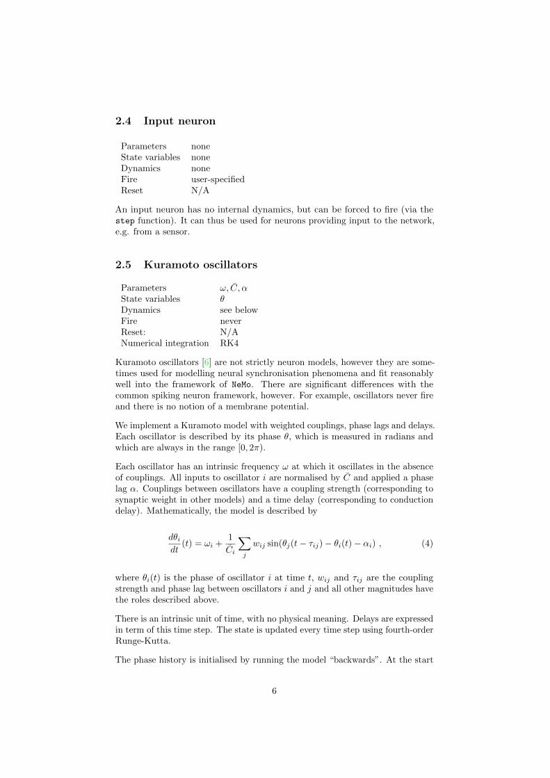
2.4 Input neuron
Parameters noneState variables noneDynamics noneFire user-specifiedReset N/A
An input neuron has no internal dynamics, but can be forced to fire (via thestep function). It can thus be used for neurons providing input to the network,e.g. from a sensor.
2.5 Kuramoto oscillators
Parameters ω, C, αState variables θDynamics see belowFire neverReset: N/ANumerical integration RK4
Kuramoto oscillators [6] are not strictly neuron models, however they are some-times used for modelling neural synchronisation phenomena and fit reasonablywell into the framework of NeMo. There are significant differences with thecommon spiking neuron framework, however. For example, oscillators never fireand there is no notion of a membrane potential.
We implement a Kuramoto model with weighted couplings, phase lags and delays.Each oscillator is described by its phase θ, which is measured in radians andwhich are always in the range [0, 2π).
Each oscillator has an intrinsic frequency ω at which it oscillates in the absenceof couplings. All inputs to oscillator i are normalised by C and applied a phaselag α. Couplings between oscillators have a coupling strength (corresponding tosynaptic weight in other models) and a time delay (corresponding to conductiondelay). Mathematically, the model is described by
dθidt
(t) = ωi +1
Ci
∑j
wij sin(θj(t− τij)− θi(t)− αi) , (4)
where θi(t) is the phase of oscillator i at time t, wij and τij are the couplingstrength and phase lag between oscillators i and j and all other magnitudes havethe roles described above.
There is an intrinsic unit of time, with no physical meaning. Delays are expressedin term of this time step. The state is updated every time step using fourth-orderRunge-Kutta.
The phase history is initialised by running the model “backwards”. At the start
6
of simulation the phase of each oscillator is thus the value specified when theoscillator was created, and previous phases have sensible values.
In the present version of NeMo the Kuramoto model should be considered ex-perimental. The present version has the limitation that the in-degree of eachoscillator is limited to 1024.
2.6 Basic synapse model
Synapses are specified by a conductance delay and a weight. Conductancedelays are specified in whole milliseconds, with a minimum delay of 1 ms andthe maximum supported delay is to 64 ms.
Synapses can be either static or plastic, using spike-timing synaptic plasticity,the details of which can be found in the next section.
2.7 STDP model
NeMo supports spike-timing dependant plasticity [8], i.e. synapses can change theirweight during simulation depending on the temporal relationship between thefiring of the pre- and post-synaptic neurons. To make use of STDP the user mustenable STDP globally by specifying an STDP function in the Configuration
object and enable plasticity for each synapse when constructing the network. Asingle STDP function is applied to the whole network.
Synapses undergoing STDP can be either potentiated or depressed. WithSTDP enabled, the simulation accumulates a weight change which is the sum ofpotentiation and depression for each synapse. Potentiation always moves thesynaptic weight away from zero, which for excitatory synapses is more positive,and for inhibitory synapses is more negative. Depression always moves thesynapses weight towards zero. The accumulation of potentiation and depressionstatistics takes place every cycle, but the modification of the weight only takesplace when explicitly requested.
Generally a synapse is potentiated if a spike arrives shortly before the postsynap-tic neuron fires. Conversely, if a spike arrives shortly after the postsynaptic firingthe synapse is depressed. Also, the effect of either potentiation or depressiongenerally weakens as the time difference, dt, between spike arrival and firingincreases. Beyond certain values of dt before or after the firing, STDP has noeffect. These limits for dt specify the size of the STDP window.
The user can specify the following aspects of the STDP function:
• the size of the STDP window;
• what values of dt cause potentiation and which cause depression;
• the strength of either potentiation or depression for each value of dt, i.e.the shape of the discretized STDP function;
7
• maximum weight of plastic excitatory synapses; and
• minimum weight of plastic inhibitory synapses.
Since the simulation is discrete-time, the STDP function can be specified byproviding values of the underlying function sampled at integer values of dt. Forany value of dt a positive value of the function denotes potentiation, while anegative value denotes depression. The STDP function is described using twovectors: one for spike arrivals before the postsynaptic firing (pre-post pair), andone for spike arrivals after the postsynaptic firing (post-pre pair). The totallength of these two vectors is the size of the STDP window. The typical schemeis to have positive values for pre-post pairs and negative values for post-pre pairs,but other schemes can be used.
When accumulating statistics a pairwise nearest-neighbour protocol is used. Foreach postsynaptic firing potentiation and depression statistics are updated basedon the nearest pre-post spike pair (if any inside STDP window) and the nearestpost-pre spike pair (if any inside the STDP window).
Excitatory synapses are never potentiated beyond the user-specified maximumweight, and are never depressed below zero. Likewise, inhibitory synapses arenever potentiated beyond the user-specified minimum weight, and are neverdepressed above zero. Synapses can thus be deactivated, but never change fromexcitatory to inhibitory or vice versa.
2.8 Discrete-time simulation
The simulation is discrete-time with a fixed one millisecond step size. Withineach step the following actions take place in a fixed order:
1. Compute accumulated current for incoming spikes;
2. Update the neuron state;
3. Determine if any neurons fired. The user can specify neurons which shouldbe forced to fire at this point;
4. Update the state of the fired neurons; and
5. Accumulate STDP statistics, if STDP is enabled.
2.9 Neuron and synapse indices
The user specifies the unique index of each neuron. These are just regularunsigned integers. The neuron indices do not have to start from zero and lie ina contiguous range, but in the current implementation such a simple indexingscheme may lead to better memory usage.
Synapses also have unique indices, but these are assigned by the library itself.Synapse indices are only required if querying the synapse state at run-time.
8
2.10 Numerical precision
The weights are stored internally in a fixed-point format (Q11.20) for two reasons.First, it is then possible to get repeatable results regardless of the order in whichsynapses are processed in a parallel setting (fixed-point addition is associative,unlike floating point addition). Second, it results in better performance, atleast on the CUDA backend with older cards (device capability < 2.0), whereatomic operations are available for integer/fixed-point but not for floating point.The fixed-point format should not overflow for synapses with remotely plausibleweights, but the current accumulation uses saturating arithmetic nonetheless.
Neuron parameters are stored as single-precision floating point.
3 Application programming interfaces
NeMo is implemented as a C++ class library and can thus be used directly in pro-grams written in C++. There are also bindings in C (Section 3.2), Python (Section3.3), and Matlab (Section 3.4). The different language APIs follow largely thesame programming model. The following sections specify the language-specificissues (linking, naming schemes, etc) while full function reference documentationcan be found in the online documentation for C++, C, and Python.
9
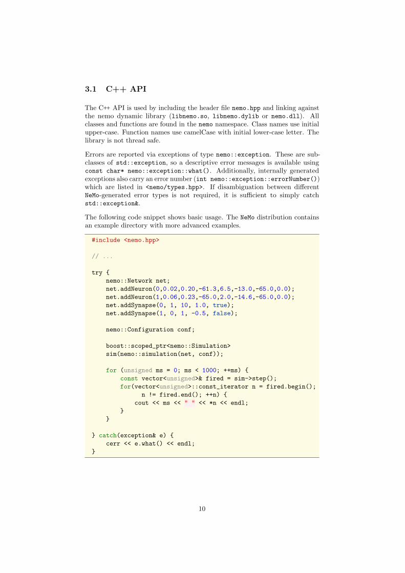
3.1 C++ API
The C++ API is used by including the header file nemo.hpp and linking againstthe nemo dynamic library (libnemo.so, libnemo.dylib or nemo.dll). Allclasses and functions are found in the nemo namespace. Class names use initialupper-case. Function names use camelCase with initial lower-case letter. Thelibrary is not thread safe.
Errors are reported via exceptions of type nemo::exception. These are sub-classes of std::exception, so a descriptive error messages is available usingconst char* nemo::exception::what(). Additionally, internally generatedexceptions also carry an error number (int nemo::exception::errorNumber())which are listed in <nemo/types.hpp>. If disambiguation between differentNeMo-generated error types is not required, it is sufficient to simply catchstd::exception&.
The following code snippet shows basic usage. The NeMo distribution containsan example directory with more advanced examples.
#include <nemo.hpp>
// ...
try {
nemo::Network net;
net.addNeuron(0,0.02,0.20,-61.3,6.5,-13.0,-65.0,0.0);
net.addNeuron(1,0.06,0.23,-65.0,2.0,-14.6,-65.0,0.0);
net.addSynapse(0, 1, 10, 1.0, true);
net.addSynapse(1, 0, 1, -0.5, false);
nemo::Configuration conf;
boost::scoped_ptr<nemo::Simulation>
sim(nemo::simulation(net, conf));
for (unsigned ms = 0; ms < 1000; ++ms) {
const vector<unsigned>& fired = sim->step();
for(vector<unsigned>::const_iterator n = fired.begin();
n != fired.end(); ++n) {
cout << ms << " " << *n << endl;
}
}
} catch(exception& e) {
cerr << e.what() << endl;
}
10
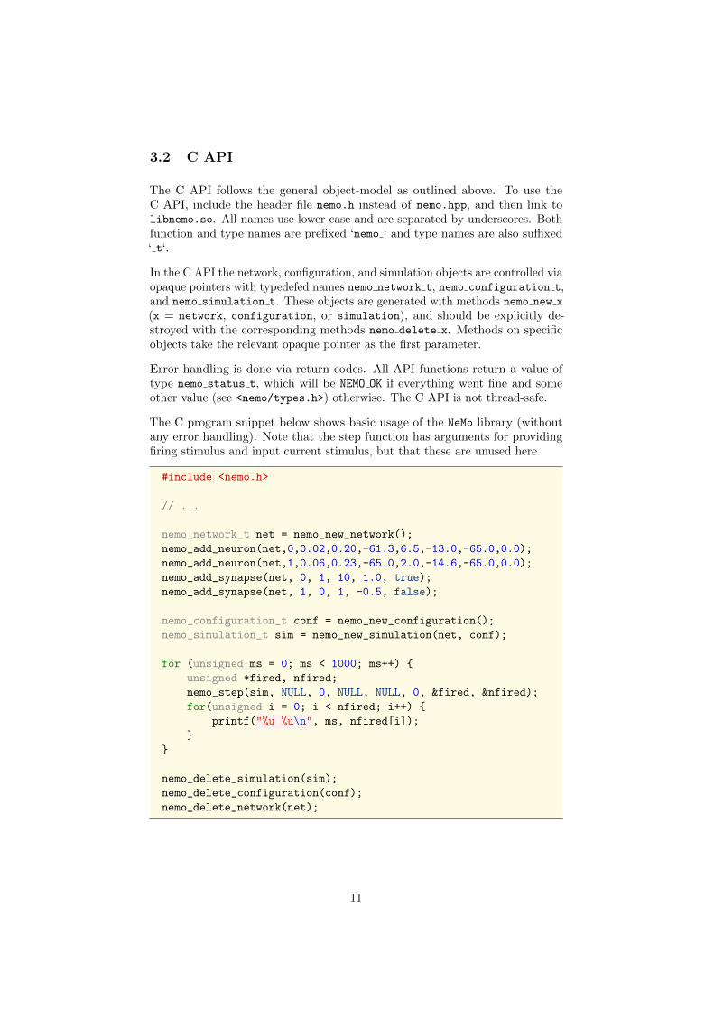
3.2 C API
The C API follows the general object-model as outlined above. To use theC API, include the header file nemo.h instead of nemo.hpp, and then link tolibnemo.so. All names use lower case and are separated by underscores. Bothfunction and type names are prefixed ‘nemo ‘ and type names are also suffixed‘ t‘.
In the C API the network, configuration, and simulation objects are controlled viaopaque pointers with typedefed names nemo network t, nemo configuration t,and nemo simulation t. These objects are generated with methods nemo new x
(x = network, configuration, or simulation), and should be explicitly de-stroyed with the corresponding methods nemo delete x. Methods on specificobjects take the relevant opaque pointer as the first parameter.
Error handling is done via return codes. All API functions return a value oftype nemo status t, which will be NEMO OK if everything went fine and someother value (see <nemo/types.h>) otherwise. The C API is not thread-safe.
The C program snippet below shows basic usage of the NeMo library (withoutany error handling). Note that the step function has arguments for providingfiring stimulus and input current stimulus, but that these are unused here.
#include <nemo.h>
// ...
nemo_network_t net = nemo_new_network();
nemo_add_neuron(net,0,0.02,0.20,-61.3,6.5,-13.0,-65.0,0.0);
nemo_add_neuron(net,1,0.06,0.23,-65.0,2.0,-14.6,-65.0,0.0);
nemo_add_synapse(net, 0, 1, 10, 1.0, true);
nemo_add_synapse(net, 1, 0, 1, -0.5, false);
nemo_configuration_t conf = nemo_new_configuration();
nemo_simulation_t sim = nemo_new_simulation(net, conf);
for (unsigned ms = 0; ms < 1000; ms++) {
unsigned *fired, nfired;
nemo_step(sim, NULL, 0, NULL, NULL, 0, &fired, &nfired);
for(unsigned i = 0; i < nfired; i++) {
printf("%u %u\n", ms, nfired[i]);
}
}
nemo_delete_simulation(sim);
nemo_delete_configuration(conf);
nemo_delete_network(net);
11
3.3 Python API
The Python API for NeMo provides an object-oriented interface that closelyreflects the underlying C++ class library. The module nemo contains the threeobjects Network, Configuration, and Simulation. The interface layer is imple-mented using boost::python, the support library of which is statically linkedin. Function names are all lower case with underscores.
Setup When installing the base NeMo library (Section 4), the Python wrapper isinstalled to a subdirectory of the main installation path (Table 1). This containsa distutils setup script, which installs the module initialization file to theappropriate location in the system’s Python installation. Run python setup.py
install to perform this installation, after which import nemo should work.Alternatively, the NeMo-related files can be left in the NeMo-specific installationdirectory. The Python path then has to be set manually to include the relevantpath from Table 1, either by setting the environment variable PYTHONPATH, orwithin a script/session by calling sys.path.append.
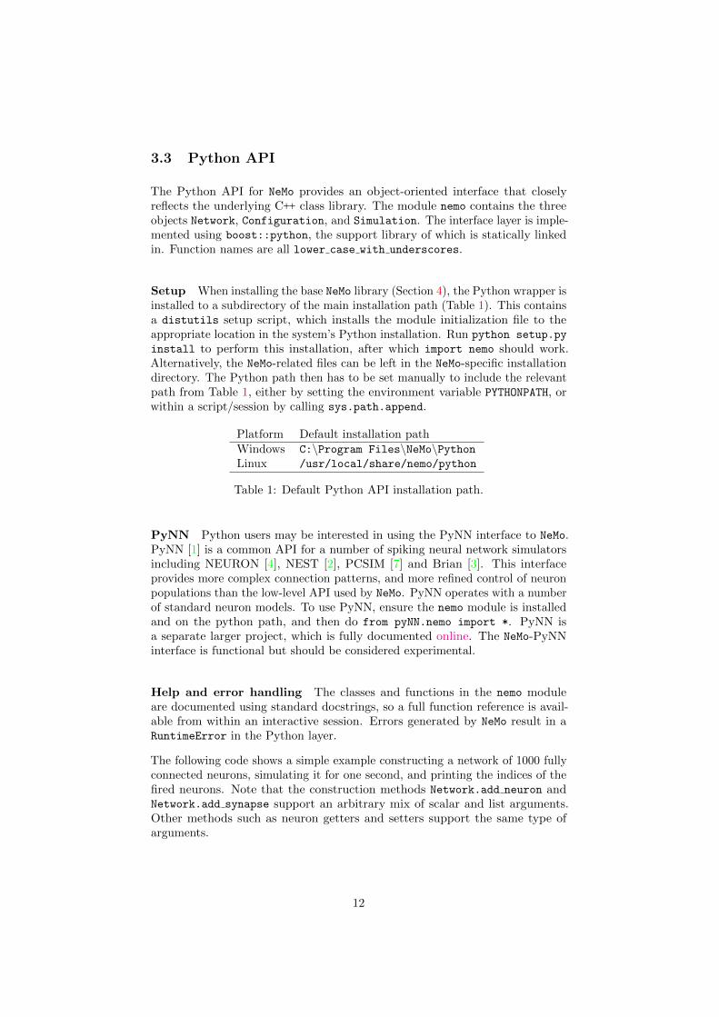
Platform Default installation pathWindows C:\Program Files\NeMo\PythonLinux /usr/local/share/nemo/python
Table 1: Default Python API installation path.
PyNN Python users may be interested in using the PyNN interface to NeMo.PyNN [1] is a common API for a number of spiking neural network simulatorsincluding NEURON [4], NEST [2], PCSIM [7] and Brian [3]. This interfaceprovides more complex connection patterns, and more refined control of neuronpopulations than the low-level API used by NeMo. PyNN operates with a numberof standard neuron models. To use PyNN, ensure the nemo module is installedand on the python path, and then do from pyNN.nemo import *. PyNN isa separate larger project, which is fully documented online. The NeMo-PyNNinterface is functional but should be considered experimental.
Help and error handling The classes and functions in the nemo moduleare documented using standard docstrings, so a full function reference is avail-able from within an interactive session. Errors generated by NeMo result in aRuntimeError in the Python layer.
The following code shows a simple example constructing a network of 1000 fullyconnected neurons, simulating it for one second, and printing the indices of thefired neurons. Note that the construction methods Network.add neuron andNetwork.add synapse support an arbitrary mix of scalar and list arguments.Other methods such as neuron getters and setters support the same type ofarguments.
12
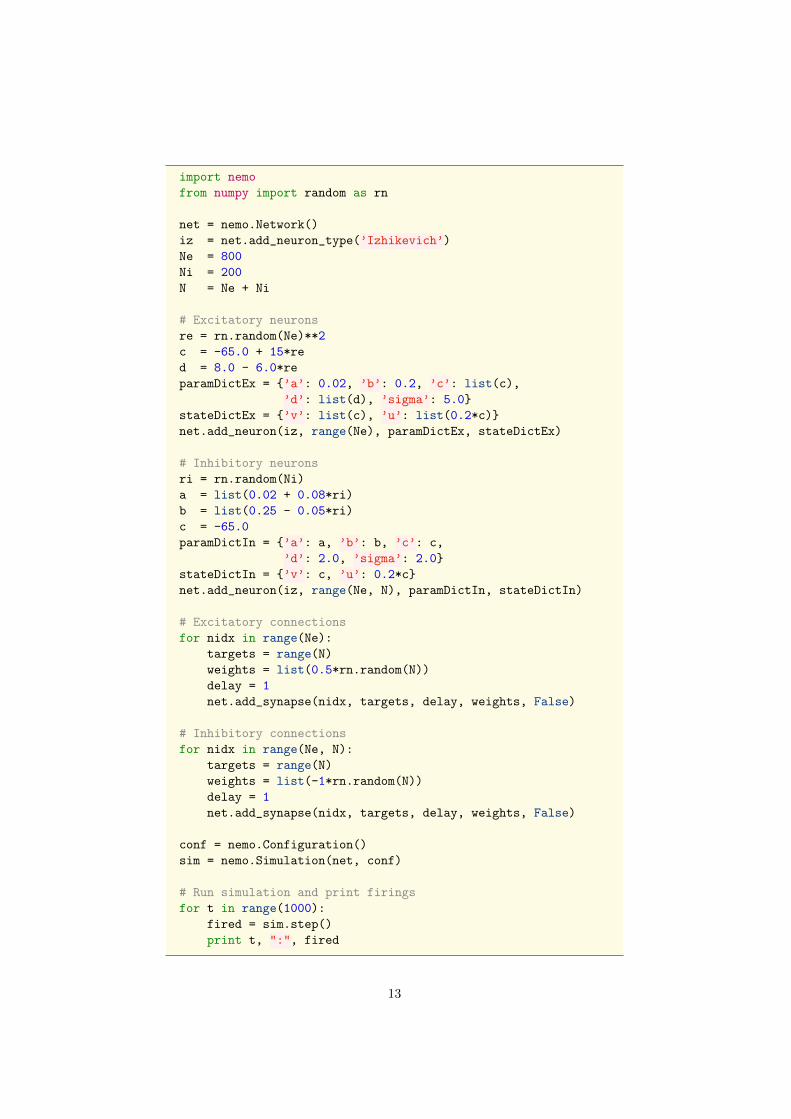
import nemo
from numpy import random as rn
net = nemo.Network()
iz = net.add_neuron_type(’Izhikevich’)
Ne = 800
Ni = 200
N = Ne + Ni
# Excitatory neurons
re = rn.random(Ne)**2
c = -65.0 + 15*re
d = 8.0 - 6.0*re
paramDictEx = {’a’: 0.02, ’b’: 0.2, ’c’: list(c),
’d’: list(d), ’sigma’: 5.0}
stateDictEx = {’v’: list(c), ’u’: list(0.2*c)}
net.add_neuron(iz, range(Ne), paramDictEx, stateDictEx)
# Inhibitory neurons
ri = rn.random(Ni)
a = list(0.02 + 0.08*ri)
b = list(0.25 - 0.05*ri)
c = -65.0
paramDictIn = {’a’: a, ’b’: b, ’c’: c,
’d’: 2.0, ’sigma’: 2.0}
stateDictIn = {’v’: c, ’u’: 0.2*c}
net.add_neuron(iz, range(Ne, N), paramDictIn, stateDictIn)
# Excitatory connections
for nidx in range(Ne):
targets = range(N)
weights = list(0.5*rn.random(N))
delay = 1
net.add_synapse(nidx, targets, delay, weights, False)
# Inhibitory connections
for nidx in range(Ne, N):
targets = range(N)
weights = list(-1*rn.random(N))
delay = 1
net.add_synapse(nidx, targets, delay, weights, False)
conf = nemo.Configuration()
sim = nemo.Simulation(net, conf)
# Run simulation and print firings
for t in range(1000):
fired = sim.step()
print t, ":", fired
13
3.4 Matlab API
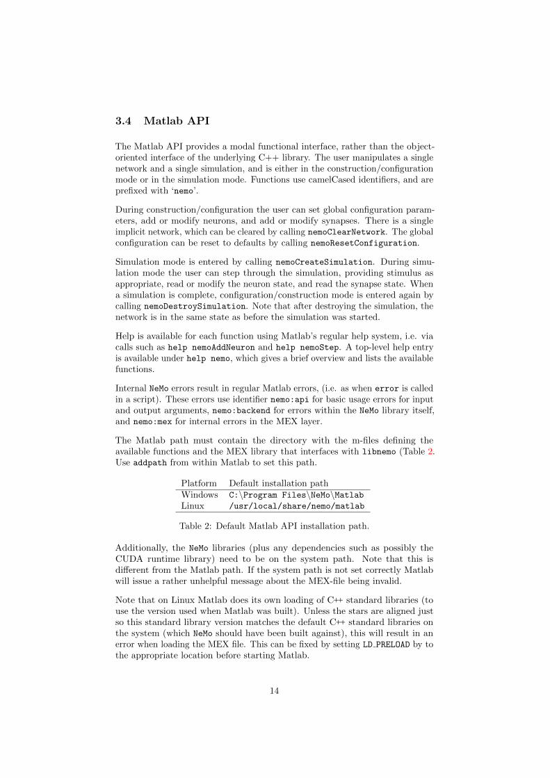
The Matlab API provides a modal functional interface, rather than the object-oriented interface of the underlying C++ library. The user manipulates a singlenetwork and a single simulation, and is either in the construction/configurationmode or in the simulation mode. Functions use camelCased identifiers, and areprefixed with ‘nemo’.
During construction/configuration the user can set global configuration param-eters, add or modify neurons, and add or modify synapses. There is a singleimplicit network, which can be cleared by calling nemoClearNetwork. The globalconfiguration can be reset to defaults by calling nemoResetConfiguration.
Simulation mode is entered by calling nemoCreateSimulation. During simu-lation mode the user can step through the simulation, providing stimulus asappropriate, read or modify the neuron state, and read the synapse state. Whena simulation is complete, configuration/construction mode is entered again bycalling nemoDestroySimulation. Note that after destroying the simulation, thenetwork is in the same state as before the simulation was started.
Help is available for each function using Matlab’s regular help system, i.e. viacalls such as help nemoAddNeuron and help nemoStep. A top-level help entryis available under help nemo, which gives a brief overview and lists the availablefunctions.
Internal NeMo errors result in regular Matlab errors, (i.e. as when error is calledin a script). These errors use identifier nemo:api for basic usage errors for inputand output arguments, nemo:backend for errors within the NeMo library itself,and nemo:mex for internal errors in the MEX layer.
The Matlab path must contain the directory with the m-files defining theavailable functions and the MEX library that interfaces with libnemo (Table 2.Use addpath from within Matlab to set this path.
Platform Default installation pathWindows C:\Program Files\NeMo\MatlabLinux /usr/local/share/nemo/matlab
Table 2: Default Matlab API installation path.
Additionally, the NeMo libraries (plus any dependencies such as possibly theCUDA runtime library) need to be on the system path. Note that this isdifferent from the Matlab path. If the system path is not set correctly Matlabwill issue a rather unhelpful message about the MEX-file being invalid.
Note that on Linux Matlab does its own loading of C++ standard libraries (touse the version used when Matlab was built). Unless the stars are aligned justso this standard library version matches the default C++ standard libraries onthe system (which NeMo should have been built against), this will result in anerror when loading the MEX file. This can be fixed by setting LD PRELOAD by tothe appropriate location before starting Matlab.
14
export LD_PRELOAD=/lib/libgcc_s.so.1:/usr/lib/libstdc++.so.6.0.13
If using NeMo installed from a binary package, ensure that the architecture(32/64-bit) matches that of Matlab. A mismatch will mean the Matlab bindingswon’t work.
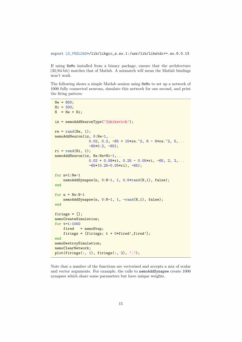
The following shows a simple Matlab session using NeMo to set up a network of1000 fully connected neurons, simulate this network for one second, and printthe firing pattern:
Ne = 800;
Ni = 200;
N = Ne + Ni;
iz = nemoAddNeuronType(’Izhikevich’);
re = rand(Ne, 1);
nemoAddNeuron(iz, 0:Ne-1,...
0.02, 0.2, -65 + 15*re.^2, 8 - 6*re.^2, 5,...
-65*0.2, -65);
ri = rand(Ni, 1);
nemoAddNeuron(iz, Ne:Ne+Ni-1,...
0.02 + 0.08*ri, 0.25 - 0.05*ri, -65, 2, 2,...
-65*(0.25-0.05*ri), -65);
for n=1:Ne-1
nemoAddSynapse(n, 0:N-1, 1, 0.5*rand(N,1), false);
end
for n = Ne:N-1
nemoAddSynapse(n, 0:N-1, 1, -rand(N,1), false);
end
firings = [];
nemoCreateSimulation;
for t=1:1000
fired = nemoStep;
firings = [firings; t + 0*fired’,fired’];
end
nemoDestroySimulation;
nemoClearNetwork;
plot(firings(:, 1), firings(:, 2), ’.’);
Note that a number of the functions are vectorised and accepts a mix of scalarand vector arguments. For example, the calls to nemoAddSynapse create 1000synapses which share some parameters but have unique weights.
15
4 Installation
4.1 Windows
The easiest way to install is by using the precompiled library (NSIS installer).This installs NeMo to C:\Program Files\NeMo, with libraries in the bin sub-directory and headers in the include subdirectory, Python bindings, Matlabbindings, and examples are stored in separate subdirectories. Note that binaryinstaller may be built against a specific version of CUDA, as well as for a partic-ular architecture (32-bit vs 64-bit). If the binary installer does not match yoursystem, building from source might be the best option.
Alternatively, the library can be built from source using cmake to generate aVisual Studio project file, and then building from within Visual Studio (seeSection 4.4). Builds in Cygwin or MSys/MinGW have not been tested.
4.2 Linux
There are no precompiled binaries for Linux, so the library should be builtfrom source using cmake (Section 4.4). By default, headers are installed to/usr/local/include; library files to /usr/local/lib; and Python/Matlabbindings, examples and documentation to subdirectories of /usr/local/share/nemo.
4.3 OSX
The easiest way to install is by using the precompiled library (PackageMakerinstaller). By default, headers are installed to /usr/include, library files areinstalled to /usr/lib, while Python bindings, Matlab bindings, examples anddocumentation are found in subdirectories of /usr/share/nemo. While theinstaller allows changing the install path, this may lead to runtime in the currentversion. Alternatively, the library can be built from source using cmake and theGNU build tools (see Section 4.4).
Installation from source in OSX is possible, but unstable. Different versions ofthe pre-existing software in an OSX system might cause different issues. Werefer the reader to the troubleshooting guide below (Section 4.5).
4.4 Building from source
NeMo relies on several boost libraries. Most of these are header-only, but thefollowing non-header libraries are also required: program options, filesystem,and date time. On Linux/OSX the libltdl is required for plugin loading. Someadditional dependencies may be needed depending on what cmake configurationoptions are set (Table 3).
The standard CMake build procedure consists of the following steps:
16
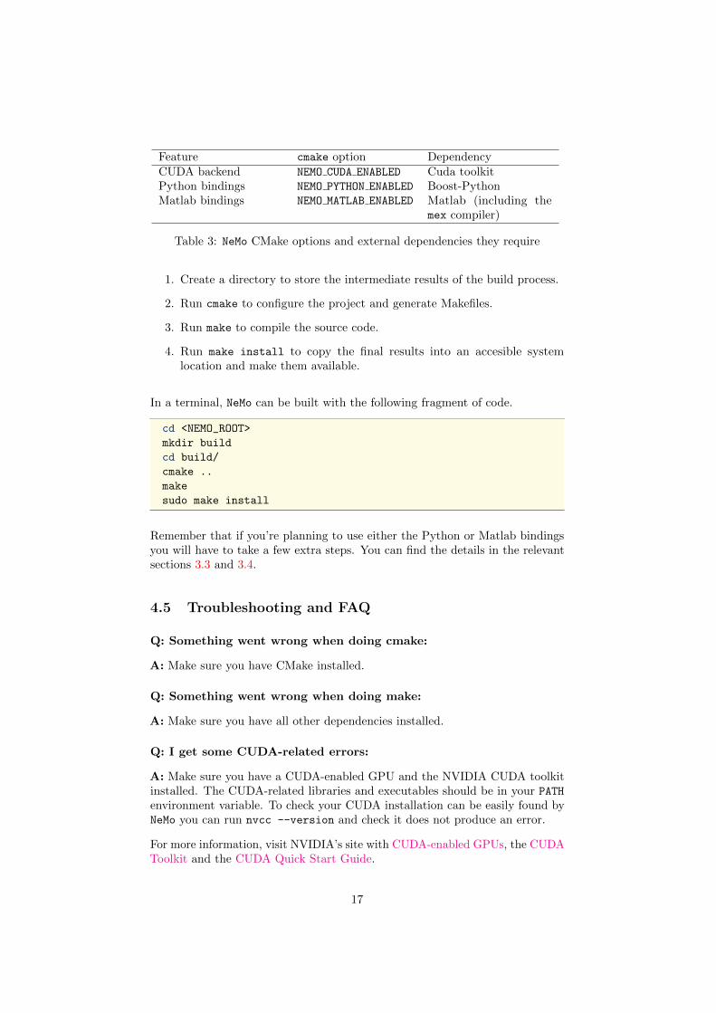
Feature cmake option DependencyCUDA backend NEMO CUDA ENABLED Cuda toolkitPython bindings NEMO PYTHON ENABLED Boost-PythonMatlab bindings NEMO MATLAB ENABLED Matlab (including the
mex compiler)
Table 3: NeMo CMake options and external dependencies they require
1. Create a directory to store the intermediate results of the build process.
2. Run cmake to configure the project and generate Makefiles.
3. Run make to compile the source code.
4. Run make install to copy the final results into an accesible systemlocation and make them available.
In a terminal, NeMo can be built with the following fragment of code.
cd <NEMO_ROOT>
mkdir build
cd build/
cmake ..
make
sudo make install
Remember that if you’re planning to use either the Python or Matlab bindingsyou will have to take a few extra steps. You can find the details in the relevantsections 3.3 and 3.4.
4.5 Troubleshooting and FAQ
Q: Something went wrong when doing cmake:
A: Make sure you have CMake installed.
Q: Something went wrong when doing make:
A: Make sure you have all other dependencies installed.
Q: I get some CUDA-related errors:
A: Make sure you have a CUDA-enabled GPU and the NVIDIA CUDA toolkitinstalled. The CUDA-related libraries and executables should be in your PATH
environment variable. To check your CUDA installation can be easily found byNeMo you can run nvcc --version and check it does not produce an error.
For more information, visit NVIDIA’s site with CUDA-enabled GPUs, the CUDAToolkit and the CUDA Quick Start Guide.
17
Remember that NeMo can also work in CPU-only mode, and will probably befast enough unless you’re doing very large simulations. You can build NeMo inCPU-only mode by deactivating the NEMO_CUDA_ENABLED option in CMake.
Q: I made changes to a CMakeLists file, but I keep getting problems:
A: CMake should automatically update the makefiles in the build folder, butdepending on where you made your changes it might miss them. To be sure,remove all the contents of the build folder and do cmake .. again. To do thisfrom command line, you can run rm -rf build/* from the NeMo root folder.But be very careful with the rm -rf command!
Q: I can’t find all these CMake options:
A: The CMake options are in the CMakeLists.txt file in the relevant folderfor each option. For example, the CMake options concerning the Matlab andPython APIs are in the <NEMO_ROOT>/src/api folder.
If you struggle to locate the options, you can use the CMake GUI to see all theoptions directly and set them on/off with a mouse click. In Linux, install it withsudo apt-get install cmake-gui and then build NeMo with cmake-gui ..
Q: I want to install NeMo in a local folder:
A: Installing NeMo in a local folder is a good idea when you’re developing somefeature or when you do not have sudo permissions in the machine you’re workingon.
To do this, the first step is to tell CMake where to place the results of the buildprocess. Add the following line in the <NEMO_ROOT>/CMakeLists.txt file, notbefore the PROJECT line:
SET(CMAKE_INSTALL_PREFIX "/path/to/install_folder")
Make sure the folder exists before calling make. We strongly recommend thatyou have a dedicated folder for this (and never use the <NEMO_ROOT> as yourinstall folder). Once the folder exists and you have modified CMakeLists.txt
you can run cmake ..; make; make install as usual (you might need toclean your build folder). This time make install will copy the include files,libraries and binaries into the folder of your choice, instead of the default/usr/local/share/nemo.
If you want to use the Python API, look for the setup.py file inside the installfolder and run it with a prefix option:
python setup.py install --prefix=/path/to/pythonAPI
Again, make sure the folder exists before running the command. Finally, tomake Python see your installation, you can set the PYTHONPATH environmentvariable to point at your new installation:
18
export PYTHONPATH=/path/to/pythonAPI/lib/python2.7/site-packages
You can verify this variable has been set correctly running echo $PYTHONPATH.Now you should be able to import NeMo in Python from any directory.
If you want to use the C or C++ bindings you will need to add the locationof NeMo’s header files and libraries to the environment variables PATH andLD_LIBRARY_PATH, respectively, or specify them manually in each invocation toGCC through the -I and -L flags, respectively.
Q: Python can’t find nemo when importing the module:
A: This is a common problem in OSX. The OSX and the Linux formats ofshared C++ libraries are the same, but they are named .dylib in OSX and .so
in Linux. This causes boost::python to lose track, so that it might not be ableto find the nemo.library although it’s in the right place. To fix this, installNeMo and the Python API as usual and then locate and rename the _nemo libraryto give it a .so suffix.
Q: I get warnings when compiling the Matlab Mex API and NeMocrashes:
A: This is a rather nasty problem that comes from (A) Matlab being propri-etary software and (B) Mathworks failing to keep up with recent versions ofGCC. Matlab’s mex functions might crash if compiled with a modern GCC.One solution is to manually install an older GCC locally (e.g. like in here)and setting the CMake variables CMAKE_C_COMPILER and CMAKE_CXX_COMPILER
to its location. You will also have to call mex with the appropriate optionmex GCC=’/path/to/gcc_binary’.
This could also be due to the mismatch of preloaded standard libraries in Matlaband NeMo. See the comment about preloaded libraries in Section 3.4.
Q: I want to run NeMo from Octave:
A: Octave, being the free-software cousin of Matlab, should handle the NeMo
Matlab API smoothly. However, the mex engines in Matlab and Octave differ,and depending on your version of Octave and GCC it might not work. Weare currently working in ensuring Octave compatibility. Please contact thedevelopers if you need an Octave API in your system.
Q: I want to write my own neuron models:
A: Easy peasy. There are a few things you have to write:
1. Write the .ini and the .h files that describe the plugin and the number ofparameters/state variables it has. Put them in <NEMO_ROOT>/src/nemo/plugins.
2. Write the CPU and/or GPU code of the actual model. Naturally, yourmodel will only be available in the backend for which you write it. Put themin <NEMO_ROOT>/src/nemo/cpu/plugins and/or <NEMO_ROOT>/src/nemo/cuda/plugins.
19
3. Incorporate it into the normal build process of NeMo by adding it into<NEMO_ROOT>/src/nemo/plugins/CMakeLists.txt. Depending on whichbackend (GPU and/or CPU) you support, you will also have to add it tothe CMakeLists.txt file in <NEMO_ROOT>/src/nemo/cpu/plugins and/or<NEMO_ROOT>/src/nemo/cuda/plugins.
4. If you’re using the Python API, add it to add_neuron function so thatyou can parse the parameter and state dictionaries correctly. Rememberthat order matters, and you should respect the ordering you specified inthe .ini and .h files.
5. Clean the build folder and rebuild NeMo.
The existing plugins should provide a good guidance in writing your own model.In all the points specified above, make sure that your plugin fits in nicely as theothers do, and use some common sense. Specially for your .cpp and/or .cu files,we suggest you to copy the .cpp and/or .cu files of the most similar existingmodel and use it as a scafold.
Q: I get an error about LTDL variables not set:
A: This error occurs when the LTDL library is not installed, not well configuredor can’t be found by NeMo. There are several ways to fix this:
1. Install libltdl. You can usually install this from the Linux packagemanager. The name of the package might vary slightly, so search the exactname with apt-cache search libltdl and then install any of them withsudo apt-get install <PKG_NAME>.
2. Build NeMo from sources. The CMake script in NeMo should download andinstall LTDL if it can’t find it. If the problem persists make sure you havea working internet connection and NeMo has the appropriate permissions.
Q: Boost cries something about STATIC ASSERTION FAILURE:
A: This is a common error in OSX. We don’t know of an elegant way around this,but it can be fixed by adding the following line in the boost/static_assert.hppfile:
template<> struct STATIC_ASSERTION_FAILURE<false> {enum{value=0};};
Somewhere in the file there should be a line with STATIC_ASSERTION_FAILURE<true>.Insert the line above below this and rebuild NeMo. This Boost file is part of aheader-only library, so there’s no need to rebuild Boost (phew).
Q: I get an error involving “sm 12”:
A: We have observed this problem in certain OSX machines with modern GPUsand recent versions of the CUDA Toolkit. It comes from a mismatch between the
20
CUDA computing capability when the NeMo GPU backend was written and themore recent versions. It can be fixed, but we don’t have an easy work-around forthis problem. Please turn off the NEMO_CUDA_ENABLED option to disable CUDAor contact the developers.
References
[1] A. P. Davison, D. Bruderle, J. M. Eppler, J. Kremkow, E. Muller, D. Pecevski,L. Perrinet, and P. Yger. PyNN: a common interface for neuronal networksimulators. Frontiers in Neuroinformatics, 2, 2008.
[2] M.-O. Gewaltig and M. Diesmann. Nest (neural simulation tool). Scholarpedia,2(4):1430, 2007.
[3] D. F. M. Goodman and R. Brette. The Brian simulator. Frontiers inNeuroscience, 3(2):192–7, sep 2009.
[4] M. L. Hines and N. T. Carnevale. The NEURON simulation environment.Neural Computation, 9(6):1179–209, aug 1997.
[5] E. M. Izhikevich. Simple model of spiking neurons. IEEE Trans. NeuralNetworks, 14:1569–1572, 2003.
[6] Y. Kuramoto. Chemical Oscillations, Waves and Turbulence. Dover Publica-tions, 1984.
[7] D. Pecevski, T. Natschlager, and K. Schuch. PCSIM: a parallel simulationenvironment for neural circuits fully integrated with Python. Frontiers inneuroinformatics, 3:11, jan 2009.
[8] J. Sjostrom and W. Gerstner. Spike-timing dependent plasticity, feb 2010.
21