Embed Size (px)
Citation preview
RADC-TR-89-1 98Final Technical ReportOctober 1989
ADr.A 2 1 7 011
NEAR-FIELD BISTATIC RCSMEASUREMENTS
The BDM Corporation
Dr. Everett G. Farr, Dr. Robeirt B. Rogers, Glen R. Salo, Theodore N. Truske
DTICELECTE .JAN 19 106
APPROVED FOR PUBLIC REMESE; D(XSRIBUTION UNLIMITED.
ROME AIR DEVELOPMENT CENTERAir Force Systems Command
Grifflis Air Force Base, NY 13441-570090 01 19 OIlT
This report has been reviewed by the RADC Public Affairs Division (PA)and is releasable to the National Technical Information Service (NTIS). AtNIS it will be releasable to the general p-iblic, intluding foreign nations.
RADC-TR-89-!98 has been reviewed and is approved for publication.
APPROVED:
KEITh D. TROTT, MAJ, USAFProject Engineer
APPROVED:
JOHN K. SCHINDLER
Director of -Electromagnetics
FOR THE COMMANDER:
JOHN A. RITZDirectorate of Plans & Programs
If your address has changed or if you wish to be removed from the RADCmailing list, or if the addressee is no longer employed by your otganization,please notify RADC (EECT) Hanscom AFB MA 01731-5000. This will assist us inmaintaining a current mailing list.
Do not return copies of this report unleso contractual obligations or noticeson a specific document require that it be returned.

UNCL&SSIPTIEDSECUWDTY CMLASTICMON 5F TmO PAGE
REPORT DOCUMMNTAT1ON PAGE %
I& IMPORT SCU•TY C/ASSOICATION IG. R--TT MrnOSUNCLASSIFIED N/A3G. SW3GIY C.ASSICAM T?ChI - IJT4~l R~~TMOTIW~AVAXASPUT OF MWoeN/A Approved for public release;N/ OASSSICATOd G 0 distribution unlilited.NlA
4. PIMFof&*4NOSGMMZA1o WoRTlhT0 AMU MO5TCG ORCAMaATION EPSIORT ftUU513T
EDM/AAO-88-0996-TR RD-TR-89-1986& W•lt OF P[W a% WA 0MAZATION 16b OFFICt 7S .MBL 'a OF I•AE•IO•ONG OFIM ATlOf4
The ED* CoTor-tion Rlose Air Developent Center (EE'T)Es. ADOOMS (C1i lty. UMand ZCo*) iG OteSOy.Sas.a PO*)
1901 Randolph Rd SEAlb•u•nerue NM 87106 Rascon AFB MA 01731-5000GaL MNA OF FUWOOIDOMteN MG F~C SYNICI. 9 FIIOJVWKT SIftFJJW n4NTSICA1 MINMl
Rm Air Development Center : P19628-86-0-0208If AOOUIS(OWy UtleM I* S04Ja OF iubaF W=OI MM
P;M=-a SNOJaCT MI TASK a 0IMPADIT no No. 'O ".o
Eansco. AFB M• 01731-5000 61102? 2305 A 60"1. -O O~azz mmOSS =O -
NEAR-FIELD BISTATIC RCS WASUL30qTS12. PERSOew1c A4THO14"Dr. Everett G. Farr, Dr. Robert B. ROJers, Glen .R. Salo, Theodore N. TrucksFinal4O POl 13.IMEC~W II OTO1FN (V~bdi Fi. AC COUNTFinAl. I FwM... ro..jT0Jj89 j October 1989 I 176
MiS SUI"P MENTARY NOTATION
N/A
So ~Near-Field ICS sessurN•at; Planar near-field scanning;9istatic radar cross-section (BRCS); Plan wave scattering
09~ I 6 trL•('rHI I AISTRACT (C&Wfto o, mml teen e IsMry WM A y AFV A meThe Final TecImical R*port presents the reaults of a feasibility Ifvestiestion of atechnique for calculating the far-field radar cross section of en obJfact basad upon usea-aurennta made in the near-field of the object. -his technique i.s -- extension of exitaplanar naar-field antenna measurement technology, and in capable of ea•muring nonostaticradar crosa section and bietatic radar cross section at both narrow end Wide angles.
Included are the detailed forzulation of the theory of near-field planer bistatic radarcross sectico measurement, and discu•sion of details of the mechanical scanner and soft-ware Implementations. The comparison of usaurernt with prediction ia presented; theagreement is excellent, and suggests that a larger scale dazonstration would be appropri-ate. Also included are concepts for reducing the amont of data reqqired from recon-structing radar cross section, and a discussion of limitations of this method of radar
crs ection measurement. (Continued ou reverse)30. 0MTx 5(lOctVAVAA8l OF AITRACT S12 A&STSACT SI01 OASSWICATIO
OON, Swm 147 eUkeR•ino MoSANG Al N. C1 OML' .UNCLASSFIED225 MFAW Of gllo~l FA&COG. 2. IIPTS AelMCOMU Im ZZ~C U SYMMMIKeith 0D. lrttza001617 377-439 IADC (ZECT)
00 Fcsm 1473. JUN 86 PSL..FegMee 0,C511 45USPCAT1,M Q! THI0PAJUNCLASSIFIED

UNCLASSM7ED
Item 19 Continued:
Specific recieommndationa are pre•ented for trclmology de•olopmuan. are that ahould bepursued to meaor this measurment technique Into a viable, operational tachnology.Anmoo those aroes are callbration, data handling, computational optinizatinn, dataanalsis., operational considerations, and additional theoretical. development.
'J9CLASSIF IED
SUMMARY
This Final Technical Report presents the re-sults of a feasibility investigation of a
technique for calculating the far-field radar cross section of an object based upon
measurements made in the near--field of the object. This technique is an extension of
existing planar near-field antenna measurement technology, and is capable of measuring
monostatic radar cross section and bistatic radar cross section at both narrow and wide
angles.
Included are the detailed formulation of the theory of near-field planar bistatic
radar cros section measurement, and discussion of details of the mechanical scanner and
software implementation. The comparison of measurement with predictions is presented;
the agreement is excellent, and suggests that a larger-scale demonstration would be
appropriate. Also included are concepts for reducing the amount of data required for
reconstructing radar cross section, and a discussion of limitations of this method of radar
cross-section measurement.
$pecific recommendations are presented for techuology development areas that
should be pursued to mature this meaurament technique into a viable, operational
technology. Among those areas are calibration, data handling, computational
optimization, data analysis, operational considerations, and additional theoretical
development. '
Accession For021S GRAAZDTIC TAB "unannoun Od DJuatlfloatio-
byDlstrub~tlac/Availability OWes
Avail and/orDist Sp•atal
• I I I I

FOREWORD
The BDM Corporation, 1801 Randolph Road SE, Albuquerque, NM 87106, is
pleased to submit this report, titled "Final Technical Report for Near-Field Bistatic RCS
Measurement," to the Rome Air Development Center as required by CDRL
DI-A--3591A/M.
This document presents a description of the work performed under contract number
F19628-6-C-0208 during the period of September 30, 1986 to March 20, 1989.
iv
TABLE OF CONTENTS
I INTRODUCTION I-i
u FORMULATION OF NEAR-FIELD THEORY Il-1
A INTRODUCTION 11-1B. SCATTERING MATRIX II-iC. MEASUREMENTS II-3D. OUTLINE OF SOLUTION 11-4E. CALCULATING P1(.,) 11--5
F. COMPUTING F2(11,A) I-7G. VECTOR COUPLING PRODUCE U1-8H. CALCULATING THE SCATTERING MATRIX 11-9
III DEVELOPMENT OF SOFTWARE TO COMPUTE SCATTERING I11-I
A, INTRODUCTION III-IB. DFT ORIGIN AND PHASE SHIFT 111-1C, DISCUSSION OF CALCULATED SCATTERING MATRIX 111-3D. GRIDDED VALUES OF k AND f- 111-4E. SIGNAL PROCESSING 111--5F. OVER-SAMPLING 111-6G. DIGITIZATION RATE 111-7H. PHASE WRAP DETECTION iHI-8I. SPATIAL FILTERING 111-15J. POWER SPECTRUM ANALYSIS 111-17
IV DESIGN AND CONSTRUCTION OF SCANNER IV-1
A. SCAN TABLE IV-iB. PROBE ANTENNAS IV-1C. SCAN PATTERNS IV-3D. MEASUREMENT CONFIGURATION IV-3E. DATA ACQUISITION SYSTEMl IV-
V COMPARISON OF MEASUREMENTS WITH SOLUTIONS V-1
A. INTRODUCTION V-IB. COHERENT BACKGROUND SUBTRACTION V-1C. DATA TAPERING V-4D. PROBE-PROBE COUPLING V-!liE. REGION OF DEFINITION V-I1F. CUT PLOTS V-16G. SUMMARY V-32
S" I ! '-" . . "' """•' •| "" '••• •-, ••,.,'--'.• ; •,I, •'V• '" •
VI DATA REDUCTION INVESTIGATION VI-1
A. INTRODUCTION VI-IB. MATRIX OPERATIONS VI-2C. FUNCTIONAL EXPANSION VI-12
VII DEFINITION OF MEASUREMENT LIMITATIONS VII-i
A. INTRODUCTION VII-lB. DATA ACQUISITION LIMITATIONS VII-1
1. Receiver Design VII-12. Data Storage V1-33. Existing Tchnology VII-5
C. WIDE-ANGLE BISTATIC RCS VII--5D. CONCLUSIONS VII-9
VIII CONCLUSIONS VIII-l
A. INTRODUCTION VIII-1B. REALISTIC RCS MEASUREMENT REQUIREMENTS VIII-2C. THEORETICAL BASIS VIII-3D. CALIBRATION VIII-3E. MEASURING THE NECESSARY DATA VIII-3F. DATA ANALYSIS VIII-6G. OPERATIONAL CONSIDERATIONS VIII-7
REFERENCES R-1
Appendix A COORDINATE SYSTEMS A-1A. COORDINATE SYSTEMS A-1B. COORDINATE SYSTEM TRANSFORMATIONS A-3C. ILLUMINATING PLANE WAVE A-4D. SCATTERED PLANE WAVE A-6E. SCATTERING CALCULATION A-7F. TRANSFORMATION OF SCATTERED WAVE A-12
Appendix B PROBE ANTENNAS B-1A. PROBE ANTENNA E-FIELD B-iB. METHOD OF STATIONARY PHASE B-3C. OPEN-ENDED WAVEGUIDE B-5D. PROBE ANTENNA CHARACTERISTIC B-15E. FAR-FIELD OF PYRAMIDAL HORN ANTENNA B-17
Appendix C SCATTERING BY CONDUCTING SPHERE C-i
Appendix D SCATTERING BY CONDUCTING DISK D-i
vi
LIST OF FIGURES
1II-1 Gain and Phase (High SNR) 111-9
IH-2 Gains and Phase (Low SNR) Ill-10
111-3 Real and Imagnary Parts (High SNR) 111-12
11--4 Res! and Imaginary Parts (Low SNR) 111-13
111-5 Difference between Real Parts (High SNR versusLow SNR) 111-14
11-6 Smoothing Filter Characteristics 111-19
111-7 Autocorrelation and PSD of Real Part (High SNR) IH1-20
M--8 Autocorrelation and PSD of Imaginary Part (HighSNR) 111-21
111-9 Autocorrelation and PSD of Real Part (Low SNR) III-22
III-10 Autocorrelation and PSD of Imaginary Part (LowSNR) 11-23
Ill-lI Signal Cleanup of Real Part (High SNR) 111-24
11i-12 Signl Cleanup of Imaginary Part (High SNR) II-25
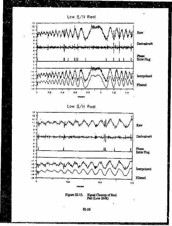
"IH-13 Signal Cleanup of Real Part (Low SNR) I1-26
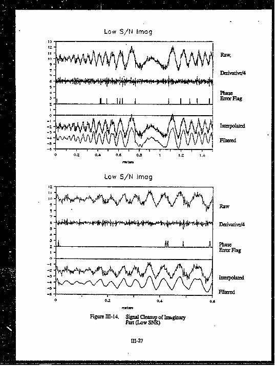
HI-14 Signal Cleanup of Imaginary Part (Low SNR) 111-27
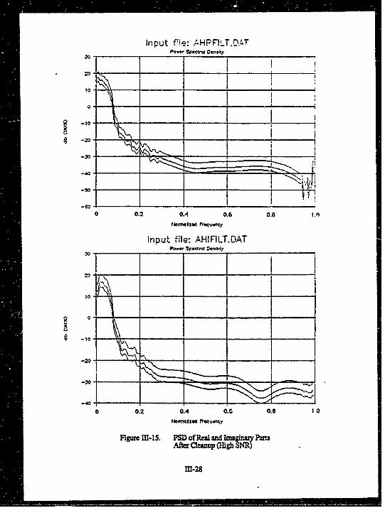
111-15 PSD of Real and Imaginary Parts afterCleanup (High SNR) Pr1-28
111-16 PSD of Real and Imaginary Parts afterCleanup (Low SNP.) 11-29
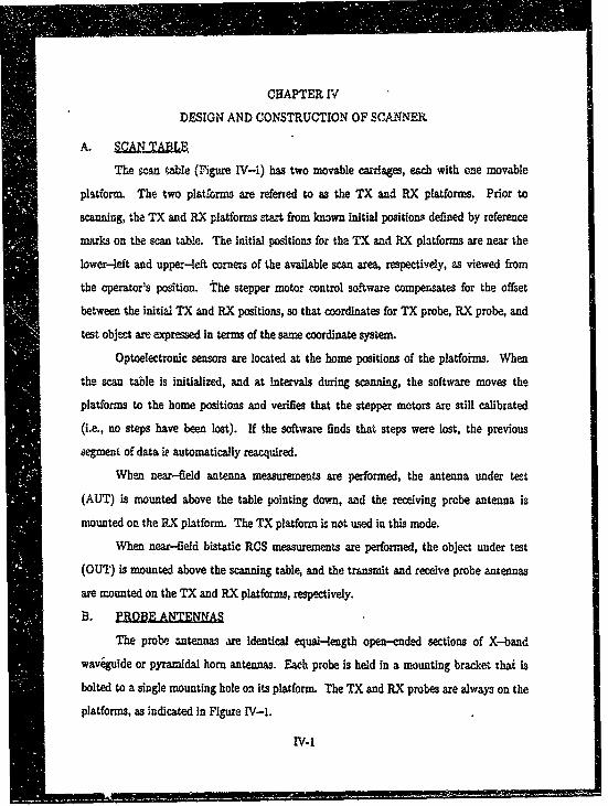
IV-I Scan Table Platforms IV-2
"V-2 Scan Patterns and Probe Oeentations WV-4
-V-3 FORTRAN Code forIAntenna Measurement ScanPattern P1-5
iV-4 FORTRAN Code for Bistatic Scan Pattern IPV-6
IV-5 Equipment Configuration IV-7
vii
IIF' • • • •}II• • ] • • ~ l ]• ..... .J F•I [• • •--III• •I • ••I• • • I•• I I, -V-7
V-1 Co-polarization Magnitude V-2
V-2 Co-polarization Background Magnitude V-3
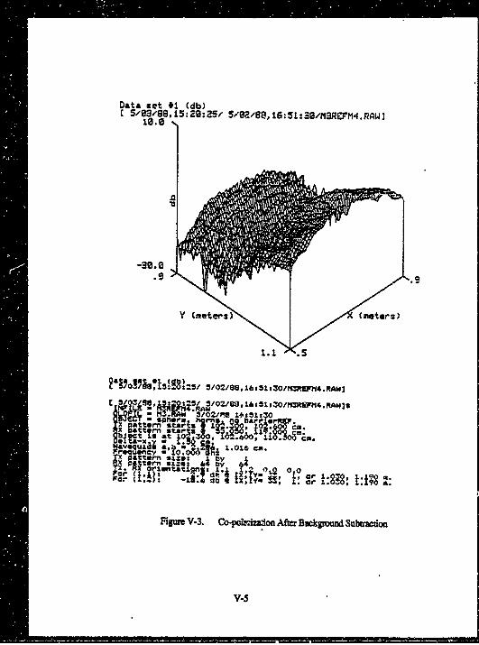
V-3 Co-polarization after Background Subtraction V-5
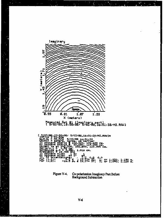
V-4 Co-polarization Imaginary Pat before BackgroundSubtraction V-6
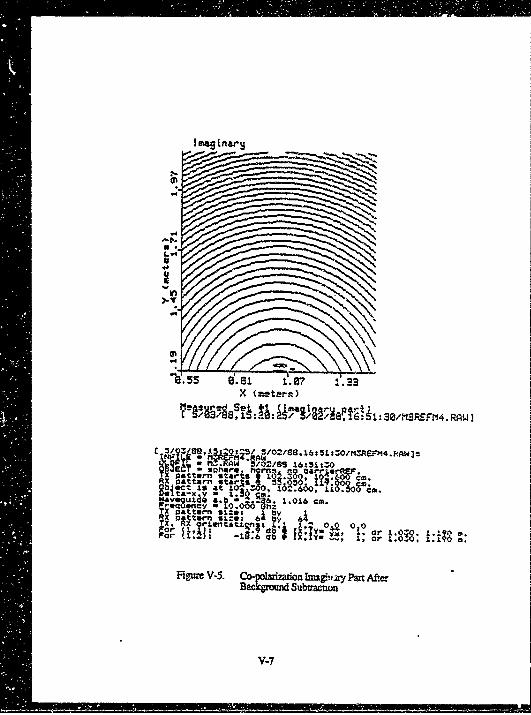
V- Co-polarization Imaginary Part after BackgroundSubtraction V-7
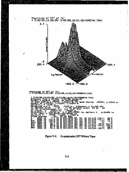
"V--6 Co-polarization DFT without Taper V-8V-7 Co-polarization DFT with Cosine Taper V-9V-8 Co-polarization DFT with Partial Cosine Taper V-It0
V-9 So DFT without Taper V-12
V-10 So DFT with Cosine Taper V-i3
V-11 So DFT with Partial Cosine Taper V-14
V-12 Sa Phase V-15
V-13 S. Phase Cut Along k. = 0 'V-i7
V-14 Predicted and Measured S0 Magnitude Cut: k= 0 V-18
V-15 Predicted and Measured S I Magnitude Cut: k=0 V-19
V-16 Predicted and Measured Sy Magnitude Cut: Ir 0 V-20
'V-17 Predicded and Measured S9 Phase Cut: kx = 0 V-21
V-18 Prediced and Measured Sy Phase Cut: kx = 0 V-22
V-19 Predicted and Measured Sp Magnitude Cut: ky = 65.4 V-23
V-26 Predicted and Measured S ,agnitude Cut: kM = 65.4 V-24
4 Paitude Cut: ky = 65.4 V-24
V-2 Predicted and Measured S. Magnitude Cut: ky = 65.4 V-25
V1-22 Predicted and Measured Sy Magnitude Cut: ky 55.4 V-26
vii
V-23 Predicted and Measured So Phase Cut: ky = 65.4 V-27V-24 Predicted and Measured S Phase Cut: ky = 65.4 .Y-28y
V-25 Predicted and Measured S. Phase Cut: ky = 65.4 V-29
V-26 Predicted and Measured Sy Phan Cut: ky - 65.4 V-30
VI1-1 Synchronous Detector Receiver Design VII-2
VII-2 Near-field Measurement Timer for Fixed ApertureAntennas VII-2
VII-3 Data Storage Requirements VII-4
VII-4 Near-field Measurement Times at 100 Mhz VII--4
VII-5 Near--field Measurement Times at 500 Mhz VII-6
VII--6 Near-field Measurement Times at I Ghz VII-6
VII-7 Near-field Measurement Times at 5 Ghz V'1-7
VII-8 Near-field Measurement Times at 10 Ghz VII-7
A-1 Coordinate Systems A-2
A-2 Scattering Geometry A-8
B-I Open-End Waveguide Geometry B-2
B-2 Ope-End Waveguide Coordinate System forFar-Field B-6
B-3 Open-End Waveguide Reference Plane B-8
V 4 Coordinate Conventions for Horn Measurements B-12
B-5 Pyramidal Horn and Coordinate Systems B-18
C-I Coordinate System for Sphere ScatteringPrediction C-2
D-1 CoordJnate System for Disk ScatteringPredictdon D-2
ix

LIST OF TABLES
VII-I Practical Target Size Limitations Versus FrequencyUsing Current Probe Scanning Techniques VII-8
x
ONE
CHAPTER I
INTRODUCTION
Radar cross-section (RCS) measurement is an important ingredient of design
verificauion and maintenance of contemporary aircraft and missile systems. RCS is
becoming more and more important for both tactical and strategic weapons systems, due in
part to increasingly sophisticated radar systems and the resulting need for low-observable
aircraft and missiles.
BDM is currently under contract to Rome Air Development Center to validate a
technique for calculating far-field monostatic and bistatic RCS using planar measurements
in the near-field of a test object. This technique, developed by BDM in 1984, is of
increasing relevance to the national need in this area, particularly in view of some of the
unique capabilities that the planar near-field technique may provide.
The goal of this contract effort is to demonstrate the feasibility of near-field
measurement of bistatic radar cross section. The proposed technical approach is divided
into six tasks which may be summarized as follows:
Task 1: Formulation of probe-corrected near-field RCS theory
Task 2: Development of software to compute scattering
Task 3: Design and construction of scanner
Task 4: Comparison of measurements with solutions
Task 5: Data reduction investigation
Task 6: Investigation of method's limitations
Those six tasks are addressed in Chapters II through VII of this final report, while
Conclusions are presented in Chapter VIII.
It is Important to realize that some of today's RCS measurement requirements
simply cannot be met with existing measurement technologies. For example, measuring
the RCS of low-observable aircraft is difficult on conventional far-field ranges: the
signature is small and hard to measure; range effects (ground and air scattering) degrade
Iol

accuracy and repeatability; airborne surveillance during long observation times
compromises security; and bistatic RCS is difficult to measure (particularly at small
angles).
BDM has been working on near-field RCS measurement and prediction concepts
since 1983. In 1984 Mike Dinallo developed and published the mathematical foundations of
a proposed near-field RCS (NFRCS) measurement approach which we called "planar
near-field RCS measurement." In 1987 Rogers and Farr published the explicit solution to
Dinallo's scattering equations and described BDM's ongoing work in near-field RCS
measurement.
Our planar NFRCS measurement technology is an outgrowth and extension of the
near-field antenna measurement theory and techniques developed by the National Bureau
of Standards (NBS) in the 1960s. The NBS theoretical ant experimental programs
demonstrated that traditional far-field antenna patterns can be calculated based upon
pattern data measured in the near-field of an antenns. These results were backed up by
extensive error analyzes and validation tests of antennas on near-field and far-field ranges.
The analyses and tests showed that patterns measured using near--field techniques are
more accurate, repeatable, and economical to obtain than patterns measured on traditional
antenna ranges. The near-field measurement facilities are also smaller than far-field
ranges and are fully enclosed, providing excellent security for sensitive military
applications. The NBS near-field antenna measurement methods are now in daily use by
most major antenna fabrication and test facilities.
Since 1984 BDM has been extending the NBS near-field antenna measurement
theory to include the near-field RCS measurement problem. Our work has been both
theoretical and experimental; we have developed the mathematics of near-field RCS
measurement and have carried on an active experimental program to validate the
mathematics. Our planar near-field RCS measurement technique is the result of this
work.
1-2

The key feature of this technique is the mathematical algorithm that allows us to
efficiently compute the RCS of an object based upon many scattering .measurements made
near the object. The measurements are conceptually easy to obtain by a computerized
data control and acquisition systen similar to the one we have prototyped in the BDM
Laboratory.
The unknown object is illuminated by a single broad-beam transmitting anunana
and the scattered signal from the object is received by one or more receiving antennas. The
transmitting and receiving antennas are in the near-field of the object (typically within a
few feet of it when using gigahertz frequencies). A computerized data acquisition system
controls where the transmit and receiving antennas are placed (using servo control) and
measures and stores the received signals. The transmitting and receiving antennas are
moved around in a plane (i.e., a planar scan pattern), so our measurement approach is
more correctly called near-fie'd bistatic RCS measurement using planar scanning.
Other noteworthy features are that bistatic measurements are feasible both at large
and small emgles, monostatic measurements are feasible, sensitivity is excellent (so
low-observables can be measured), and the measurement facility is totally enclosed (which
enhances security).
1-3
CHAPTER I
FORMULATION OF NEAR-FIELD THEORY
In this chapter we present the analysis of near-field bistatic scattering data. This
analysis is based upon Dinallo's [16] formulation of bistatic scattering in terms of the plane
wave scattering matrix. Note that for the bulk of this section we Earry out the
mathematics in the unprimed coordinates of the object under test.
B. SCATTERING MATRIX
The goal is to calculate fcr an arbitrary object a scattering matrix
I .... [ ~11100A') Ii1a ('I)
I I11(k'~ ~l)- [ 111 110')Il0(U'))
which describes the scattering of an incident plane wave by that object, and
-x6k + kay + k,6,"6xx+ yy + ,zz
It is worth noting explicitly that the elements of the scattering matrix . 11(•,l) are
specified by means of two polarization-related indices and two propagation vectors. For
example, l1180 (k,i) refers to the 0--component of the angular spectrum of the wave that is
scattered when the object is illuminated by the 0--component of the angular spectrum of
the incident wave. The incident wave has propagation vector I, and the scattered wave
has propagation vector ;. Taking all four elements together, il(k,1) specifies how the 0
and 0 components of the angular spectrum of the Incident wave I are scattered into 0 and
S components of the angular spectrum of a scattered wave k.
The incident and scattered waves are generally a superposition of plane waves which
we will model as a ontinuum of plane waves. A complicated wavefront illuminating the
object may be decomposed into a spectrum of plane waves. Measuring the transverse
components Eix and E.y of that E-field in some plane, such as z = zo, the angular
n-I
spectrum (of plane waves) is the Fourier transform in the x-y plane
Il() = Ii 9(i)• 9 + 1()
-J J () e d',
where
r'=rxi + r. + ze~.The multitude of plane waves that makes up that angular spectrum of incident plane waves
is scattered by the object, yielding an infinity of emergent plane waves whose angular
spectrum is
!2(') = WN+V06= 18A [18A I, ')I,(i,•,O(~~~11j',I) I1100(M,) J" ~~)],,I
Note that the 9- and #-componeats of the angular spectrum of the scattered plane
waves are a linear combination of both the 9- and the 0-components of the angular
spectrum of the incident plane wavs.
For a source at 'r having angular spectrum I1(t), the scattered angular spectrum at
the origin is denoted by F(*1,ý), where
P 1 4,•.,) _.[F OO• •,S ) '
F,9(;1,k)'Fo'l,¢ti) I u•kT][ , "LI I#rik II
(As written here, P(;14) Is related directly to the samp ig plane coordinates rather than
the object coordinates.) The far-f6eld scattered I at 4 is calculated with the results from
a previous section. Hence,
ts-(;2) =-2ko e+ ';2h
s2 r2 '2where i is parallel to ' 2" If the incident wave I in fact planar, then the angulr spectrum
..-2
of the incident wave Is[I101and the Integral above reduces to a matrix multiplication. The far-field scattered E-field
is
C. MEASURE
Given illumination of the test object by the transmit antenna in transmit
orientation #1, we will first calculate the 0- and O-components of the scattered angular
spectrum over the area scanned by the receive probe antenna In order to calculate the
scattering matrix Next, the transmit probe antenna is rotatod 900 to Illuminate the test
object with a different angular spectrum of plane waves, and we then repeat the
measurements and calculations In order to determine the $-- and --components of the
scattered angular spectrum for this second transmit probe antenra orientation. From these
two sets of data, we can calculate the manner In which the test object scatters the 0- and
O-components of the incident wave into the 0-and O-components of scattered waves.
The laboratory meaurements for bistatic near-field scattering consist of gain and
phase measurements made by a receive probe as it Is swept through a pattern of probe
locations. The receive probe scan pattern is swept repeatedly (and gain and phase
measurements made) for a set of transmit probe locations, as the transmit probe itself steps
through a set of locations in the transmit probe san pattern.
The transmit probe and receive probe we use are Identical, although they need not
be so. The receive probe's receiving characteristic
1o0(0) '= 110 0(k)
U-3
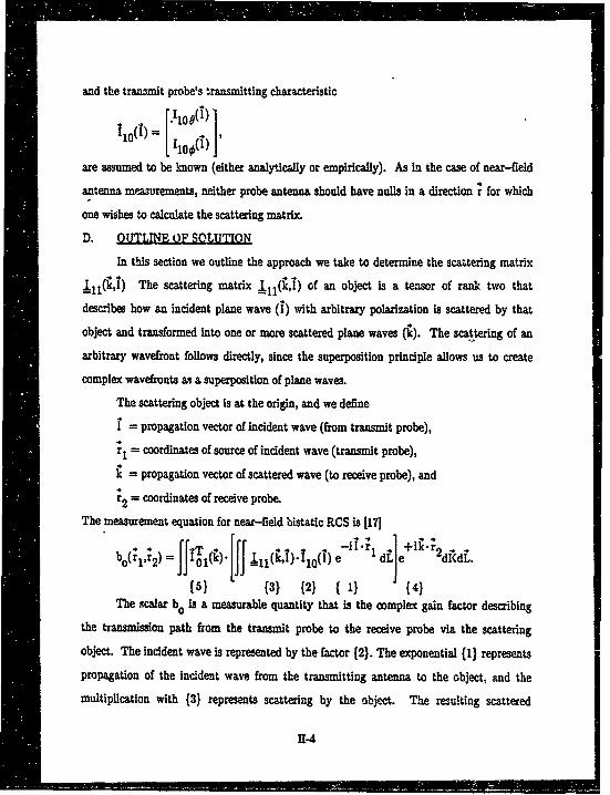
and the transmit probe's transmitting characteristic
110(l) =i109(b)I 1,1 0 0(b
are assumed to be known (either analytically or empirically). As in the case of near-field
antenna meaaurements, neither probe antenna should have nulls in a direction * for which
one wishes to calcuate the scattering matrix.
D. OUTLINE OF SOLUTION
In this section we outline the approach we take to determine the scattering matrix
_11(M,) The scattering matrix o11(•,) of an object is a tensor of rank two that
describes how an incident plane wave (1) with arbitrary polarization is scattered by that
object and transformed into one or more scattered plane waves (k). The scattering of an
arbitrary wavefront follows directly, since the superposition principle allows us to create
complex wavefronts as a superposition of plane waves.
The scattering object is at the origin, and we define
= propagation vector of incident wave (from transmit probe),
ri = coordinates of source of incident wave (transmit probe),
k= propagation vector of scattered wave (to receive probe), and
r2 = coordinates of receive probe.
The measurement equation for near-field bistatic RCS is [17]
o J12) 01(i). [JJ ~11(0,!0t10(l) e 1 dL] e 2 di dL.
{5} {3} {2} { 1} {4}The scalar bo is a measurable quantity that is the complex gain factor describing
the transmission path from the transmit probe to the receive probe via the scattering
object. The incident wave is represented by the factor {2}. The exponential {1} represents
propagation of the incident wave from the transmitting antenna to the object, and the
multiplication with {3} represents scattering by the object. The resulting scattered
H-4
~~ I ----- • - n i = =
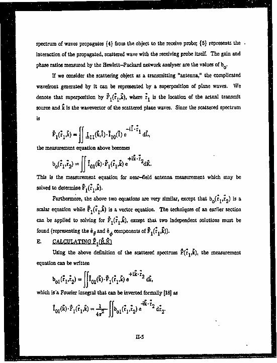
spectrum of waves propagates {4} from the object to the receive probe; {5} represents the
interaction of the propagated, scattered wave with the receiving probe itself. The gain and
phase ratios measured by the Hewlett-Packard network analyzer are the values of bo-
If we consider the scattering object as a transmitting "antenna," the complicated
wavefront generated by it can be represented by a superposition of plane waves. We
denote that superposition by P1,(G,), where 'r is the location of the actual transmit
source and k is the wavevector of the scattered plane waves. Since the scattered spectrum
is
Pi(Oi•) = 1J 10,101).I00) e *dL,
the measurement equation above becomes
b 1 -f t 0 1 (k).(lk) e22 dK.
This is the measurement equation for near-field antenna measurement which may be
solved to determine PIG'1,i).
Furthermore, the above two equations are very similar, except that bo(l,r 2 ) is a
scalar equation while Fl(rlrk) is a vector equation. The techniques of an earhler section
can be applied to solving for 1(1) except that two independent solutions must be
found (representing the e0 and & components of PI(ri,)).E. ,CALOULATTNG iI~
Using the above definition of the scattered spectrum P(rl,k), the measurement
equation can be written-~ ii'; 2 di
bol(,;2) = m1 0 1().N 1("1 ,) e+ d2
which is'a Fourier integral that can be inverted formally [18] as
rr e dr2
10(0 16 S)= 4... ... bol. 2) e k 2 • •2-
H-5
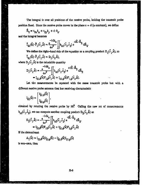
The Integral is over all positions of the receive probe, holding the transmit probe
position fixed. Since the receive probe moves in the plane z = d (a constant), we define
r%&2=r + r2yi, + d'
and the integral becomes -idk z. r i .k Jbol(rlr2 ) e A2
We define the right-hand side of the equation as a coupling product DI(li), soi ;~10( 0 4 16' 14•'I) = Dl(6l')'
where D1(r,4) is the calculable quantity
D0 )-= ---. • b 1 2) e dR2
A r 4JJ+= IO1 )F1•;1 ,•) + 0()F (li.
Let the measurements be repeated with the same transmit probe but with a
different receive probe antenna that has receiving characteristic
I01 •(k) J
obtained by rotating the receive probe by 90& Calling the new set of measurements
b,2(1,r2), we can compute another coupling produ'ct D2( as
D2('S)= e4- -Jjbo2 (rj,r2) e d•.
- I•I~)FI•I,•) + l()F (• )
If the determinant
Al(O) - 01),)10(1) -16(0)I010)
is non-zero, then
H1-6
k) --'r
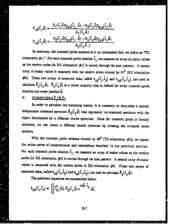
F1(•,• fiD1(1•I1(1 r - D2('l,i)6I0'1•(p•)
_ A1 (;1,• )Fl1(01,0) = D2(1,)010(1 , 1) 0 1;,)•6;•
In summary, the transmit probe antenna is in an orientation that we define as "TXorientation #L." For each transmit probe location ' we measure an array of scalar valuesas the receive probe (in RX or.entation #1) is moved through its scan pattern. A secondarray of scalar values is measured with the receive, probe rotated by 900 (RX orientation
#2). These two arrays of measured data, called bo1('rlr 2 ) and bo2(r 1,r2), are used tocalculate ( ) (-,) is a vector quantity that is defined for every transmit probe
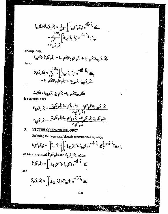
location and every possible ;.F. COMPUTINQ . i-'£
In order to calculate the scattering matrix, it is necessary to determine a second,independent scattered spectrum P2(1',) that represents ',he scattered spectrum with theobject illuminated by a different aource spectrum. Since the transmit probe is linearlypolarized, we can create a different source -pectrum by rotating the trunsmit probe
antenna.
With the transmit probe antenna rotated by 900 (TX orientation #2), we repeatthe entire series of measurements and calculations described in the previous section.For each transmit probe location ',, we measure an array of scalar values as the receiveprobe (in RX orientation #1) is moved through its acan patterr. A second array of scalarv3lues is measured with the receive probe in RX orientation #2. These two arrays ofmeasured data, called bo3(r1 ,'2 ) and bo4( 1r,* 2), are imed to calculate r
The pertinent equations are summarized below-
o3(*1,2)= IJ01(6)'F2(½1ý) e4 d ,
11-7
'01(')-P2-;j J(r 1 r2) e iir2 '
or, explicitly,
Aiso
rd rr
is Rnaz-zero, then
G. VE-CTORL COUpirnPR, TYReferring to the general b~swi~c mmnlemwet equation
2 f0M ~fJf1,(10) -11 0(f) dl.. 2ddwe have calculate ýIrý and f2 (r',k), whre .
and-f 11u.10f it;1d
kI -JiO')e if1 Id4

are Fcurier integrals that may be Inverted to give
I . . I Fjrl"( ) e1 r d;,_1110,1.0io~b • 4- P,(I l e2•' t. d~rl
This time the lntegr4s are over all positiont of the transmit probe, holding 'be
receive probe posi;ion fixed. Since the transmit probe moves In the plane z d, letAI-- rlxex + r ly~y + d, i2,
and the Integrals become
S!uc•,•),•oCii11 4-T 'j 1(r,t) e dR1
I 1I(kJ)1 0(f) - " " •2(ri.) e d. 1.
We define a pair of veclor coupling products (ij,) and •(•,,) a,
-. idl e r - d
Q(f) --77 j 2(jj, e d-v
so thit we can write1 (ij) .11oCf) = ij-
H. _QALIULT 'i E = •'( 1 M).
Exp,.iilng the above eqnuation In cwmpor.nts and dioppiag the expiiJt (lJ)
dependence,
[0 0 is I 110 9 jI O
0 0 1 3 0 i o 1 1 0 0 r4 0
11-9
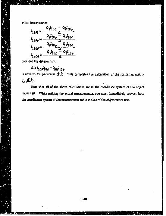
wA& his solutions:
I110o Q910
i1 = QA.00o -, QF100
_QAioO - W100
provided the determinantA 3 11oiioo- Iiohioo
is nc'wo for paxticular (;,I). This completes the calculation of the scattering matrix
Note that all of the above calculations are In the coordinate system of the object
under test. When making the actual measurements, one must immediately convert from
the ccordlnatm systew of the measurement table to that of the object under test.
-- I0

CHAPTER IIIDEVELOPMENT OF SOFTWARE TO COMPUTE SCATTERING
A. INTBODU1rTION
The software to perform the scattering ciculations is a straightforwardimplementation of the algorithm presented in the previous chapter. The heart of thesoftware is the two-dimensonal fast-Fourier transform subroutine; a number of suchsubroutines are available in the open literature.
There are a number of software issues stemming from the discretization that isimplicitly employed to calculate diserete equivalents to continuous integrals. These issuesare discussed in the following sections.
B. DFT ORIGIN AND PHASE SHIFTIn this section we discuss sampled-data evaluation of Fourier intgrals by the FFT
algorithm. For rigorous discussion, refer to the literature [12].
Numerical evaluation of integrals of the form
SH(W) = f-h(t) 'PAt dt
is feasible for bandlimited h(t) using sampled data and discrete Fovrier transformtechniques. The continuous function h(t) is sampled at Intervals of bt chosen by Nyquist's
criterion. The sampled h(t) is a finite sequence
{h'(n) - h(t) I t a to+ (a-1) 6t, nl, .... N}3 h'(I),h,(2),....h.(N)
which is implicitly periodic in n with period N. Thi DFT of h'(n) isN , 1k-l
F.'(k)= h'(n)e k ... N
where (for even N)
&as2z
•.,,.,,.....,•_ ..... .•- ,,. ... .4. ,,- ...... -- ,,,..,,,•,,,. • ...........
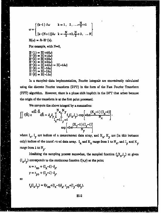
H(w) = bt.H'(k).
For example, with N=8,
H-i = H+O&H, 2 =H 1&~H, 3 = HE+25)H'4 = H(+36)H'5 =H, ) --= H(-4&a)H, 6 H:--'•
7) = H(-2,w)H'8 =HC-I&)
In a sampled-data implementation, Fourier integrals are conveniently calculated
using the discrete Fourier transform (DFT) in the form of the Fast Fourier Transform
(FFT) algorithm. However, there is a phase shift implicit in the DFT that arises because
the origin of the transform is at the first point processed.
We compute the above integral by a summation:NiKNy l" (Ki--1) (Ii-l)j
eIl= a (K--1) (1 f -1)x
where 1., 1y are indices of ameasurement data arry, and Kx, Ky are (in this instance
only) indices of the transf ra-ed data array. 1. and K. range from 1 to Nx, and Iy and Ky
range from 1 to Ny.
Idealizing the sampling procem somewhat, the sampled function fsIX,Iy) at given
(Ic,) corrw-s to the continuous function f(xy) at the point
x = x + (N-i)'8 x,
y=r yo + (ly7;Y
so
11.-2
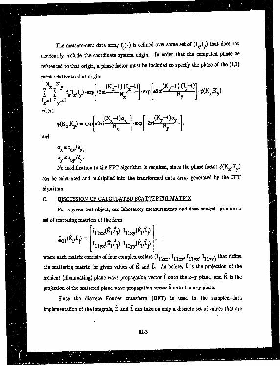
The measurement data array f,(.) Is defined over some set of (1xIy) that does not
necessarily include the coordinate system origin. In order that the computed phase be
referenced to that origin, a phase factor must be included to specify the phase of the (1,1)
point relative to that origin:N~ Ny 8 I~~.x (Ki 1) (Ix-'1)x[* (Y-1)1-)
xj= ly 1
where
K e .(K x--)a exp[*2x.e (Kx r -)a,
and
&y roy/$y.No modification to the FFT algorithm is required, since the phase factor XK,,Ky)
can be calculated and multiplied into the transformed data array generated by the FFT
algorithm.
C. D2SCUSSION OF CALCULATED SCATTERING MATRIX
For a given test object, our laboratory measurements and data analysis produce a
set of scattering matrices of the form
where each matrix consists of four complex scalars (llxx, Il xy, y I11yy) that define
the scattering matrix for given values of R and L. As before, L is the projection of the
incident (illuminating) plane wave propagation vector I onto the x-y plane, and K is the
projection of the scattered plane wave propagatlon vector ' onto the x-y plane.
Since the discrete Fourier transform (DFT) is used in the sampled-data
Implementation of the integrals, R and L' can take on only a discrete set of values that are
111-3
determined by the measurement grid size, the spatial sampling interval &, and the "rules"
of the DFT. Fourier interpolation can be used to increase the resolution of the grid of
values of R and L.
D. gRIDDED VALUES OF R AND
Suppose the transmit probe scan pattern is a square consisting of Nt. points on a
side, with spatial sample interval &- The propagation vector of the transmitted wave (i.e.,
the plane wave that is incident upon the test object) is denoted by
1= 6. + ly6 + 1,6,
and its projection onto the x-y plane is
L = lx6x + ly6y.• Then the x- and the y-components of I take on the discee values
The the -and x the-opoet of take on. thNiceevleX r Nx_ N- tx ' & 0...Ntx
I yj= &t j ---02"'i
where& 2•
tx tx
is the spacing between adjacent samples in "k--space. The maximum magnitude that 1.
or ly can have is
Ilxlmax -1y -a'-
Howa-ver, l and Iy are constrained by the a requirement that Iz be real,
since
+l I A
and propagating waves correspond to those T for which 1. Is real. If 1x or ly gets too large,
1z becomes imaginary, so we requie.
M-4
Since is the highest spatial frequency that can be present due to propagating
waves, it is the Nyquist frequency [13] of the signal to be sampled, and the required
sampling Interval is A/2. If the sample interval is indeed $, = A/2, the domain of valid
(Ixl) Is a circle in the (ij) plane that is exactly inscribed in the square defined by
-2. : Ntx1 Nt N~ tx1 I
so a fraction L•=i21% of the computed IlXjy! Is not useful to us.
A similar situation exists with regard to the range of values of the propagation
vector of the scattered plane wave. Suppose the receive probe pattern is a square with Nrx
points on a side and spatial sample interval &- The propagation vector of the scattered
wave is denoted by
K = + ky y +
and its projection onto the x-y plane is
kik.a + ky~.The x- and the y-components of i take on the discrete values
N
jk . 2 rx&rx j 01,2 ....Nr
where2 7
&rx N 6
Ik.1max Iky = "' sandk2 + k2<[2v]
E. SIGNAL PROCESSING
Conservative signal processing technique calls for using a sampling interval smaller
than the A/2 dictated by the Nyquist limit. In the present instance, the physics of the
wave propagation very effectively bandlinmts the signal by Imposing a very sharp cutoff for
M-5I
spatial frequencies beyond 1/A. This is in contrast to typical signal acquisition scenarios in
which a signal generally has components above fNyqui't; there one must use a sharp cutoff
filter and in addition sample at a somewhat higher rate than the Nyquist theorem requires.
We conclude that one should probably use & < A/2 by perhaps 5% or so.
Given the good A/D resolution (12 bits), adequate floating-point precision and
dynamic range (I.E.E.E. standard floating-point format), and a relatively quiet
measurement location, we ignore some of the common reasons for sampling at above the
Nyquist frequency, namely quantization and numeric dynamic range.
Since the experimentally-determined scattering matrices are defined at discrete
values of K and L, it is convenient to construct one's theoretical models of scattering such
that the precise values of R and L calculated by the analysis software can be automatically
plugged in to yield the theoretical scattering values. From an algorithmic standpoint this
corresponds to implementing the theoretical or numerical model of scattering as a
subroutine that has as input the values of K and i for which a theoretical prediction is
needed.
F. OVERAMPlLING
Under ideal conditions the gain and phase signals from the network analyzer need to
be sampled only at A/2 intervals (or slightly more often if one is near the reactive
near--field of the test object). In this application we oversample by a factor of ten.
Reasons for this are (1) noise generated in the electronics for gain and phase detection
smears out the spectral content of the signal being measured; (2) a general rule of thumb in
digitizing and processing noisy signals is that one should digitize at five to ten times the
Nyquist rate; (3) filtering techniques can be used to reduce the (uncorrelated) noise on the
signal; and (4) non-linear filtering techniques can be used to detect and correct invalid
phase measurements.
The invalid phase measurements occur because the phase detection circuit in the
network analyzer updates its output asynchronously with respect to the A/D converter, so
ffl-6
it is possible for the A/D to sample the phase when the circuit is "wrapping" around from
+180 to -180 degrees (or vice versa). Measuring extra points allows us to detect and
correct the invalid phase values. Spatial filtering to improve sigal-to-noise ratio (SNR)
is also practical when oversampling is performed.
The figures in this section were constructed using measured data from two x-axis
scans (made on 6/4/87) of 10 Ghz bistatic RCS from the 6-inch aluminum sphere. The
TX probe was held stationary, and the RX probe was scanned in the +x direction using a
200 hz digitizing clock and the usual probe velocity of 29.8 cm/sec. Sample interval is
calculated as 0.149 cm, corresponding to oversampling by a factor of ten at 10 Ghz.
The probes were open-end X-band waveguide with absorber collars to limit
low-angle radiation and an absorber barrier between the RX and TX probes to limit direct
probe-to-probe coupling. The TX probe was driven with a 20-watt (nominal)
traveling-wave tube (TWT) amplifier, and a preamplifier was used on the RX probe.
A high SNR scan was obtained using maximum drive to the TWT amplifier. A low
SNR scan was obtained immediately after the high SNR scan but with the TWT drive level
reduced by 15 db. Additional measurement noise was introduced by the lowered reference
channel signal at the network analyzer.S G. DIGITIZATION RATU
Since the quantity of data required by the near-field technique is already
formidable, it is preferable to store the minimum number of values necessary for the
reconstruction of the scattering matrix. The signal being measured contains no
components above spatial frequency
nan= cycles/meter,
so digitizing the signal at a sampling frequency of 2/A samples/meter would theoretically
capture all of the spectral content of the signal. For reasons mentioned above, digitizing at
ten times this rate is more appropriate, so we choose
' s samples/meter.
M[-7
Then
-, 6 .4 meter/sample
and
'Nyquist = cycles/meterIs the highest spatial frequency that can be deWcted without abasing.
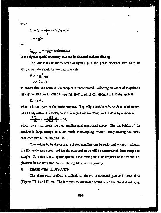
The bandwidth of the network analyzer's gain and phase detection circuits is 10
kHz, so samples should be taken at intervals&>> 1
>> 0.1 ms
to ensure that the noise in the samples is uncorrelated. Allowing an order of magnitude
leeway, we set a lower bound of one millisecond, which corresponds to a spatial interval
& = v A,
where v is the speed of the probe antenna. Typically v = 0.30 m/s, so & - .0003 meter.
At 10 Ghz, A/2 = .015 meter, so this & represents oversampling the data by a factor of"•2 .015 m .
which more than meets the oversampling goal mentioned above. The bandwidth of the
receiver is large enough to allow much oversampling without compromising the noise
characteristics of the sampled data.
Conclusions to be drawn are: (1) oversampling can be performed without reducing
the RX probe scan speed, and (2) the measured noise will be uncorrelated from sample to
sample. Note that the computer system is Idle during the time required to return the RX
platform for the next scan, so the filtering adds no time penalty.
H. PHASE WRAP DETEMTIO
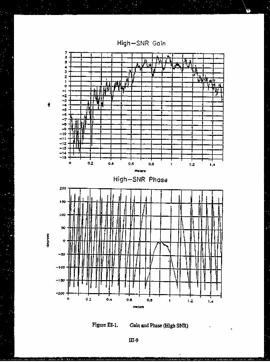
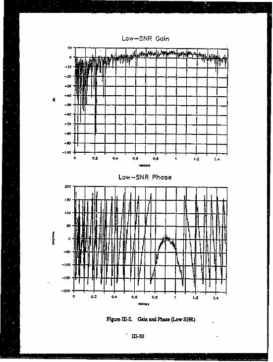
The phase wrap problem is difficult to observe in standard gain and phase plots
(Figures Ill-1 and mI-2). The incorrect measurement occurs when the phase is changing
M-4
High-SNR Gain
H-IIf I
-14
0 0_ 0.4 OAS 0.8 1 t.2 1.A
High-SNR Phase
-IS 4:ftoo-t
Fiue001,Gi n hse(ihSR
01-
Low-SNR Gain
0 OA0. 0.6 0.0 1 . 1.4
FiLow-S.. aN an Phase(LwS)
lm.1
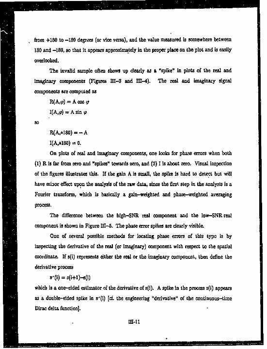
from +180 to -180 degrees (or vice versa), and the value measured is somewhere between
180 and -180, so that it appears approximately in the proper place on the plot and is easily
overlooked.
The invalid sample often shows up dearly as a "spike" in plots of the real and
Imaginary components (Figures 111-3 and MI--4). The real and imaginary signal
components are computed as
R(A,,p) = A cos •p
-(A,p) = A sin
so
R(A,*180) = - A
I(A,180) 0.
On plots of real and imaginary components, one looks for phase errors when both
(1) R is far from zero and "spikes" towards zero, and (2) I is about zero. Visual inspection
of the figures illustrates this. If the gain A Is small, the spike is hard to detect but will
have minor effect upon the analysis of the raw data, since the first step in the analysis is a
Fourier transform, which is basically a gain-weighted and phase-weighted averaging
proces.
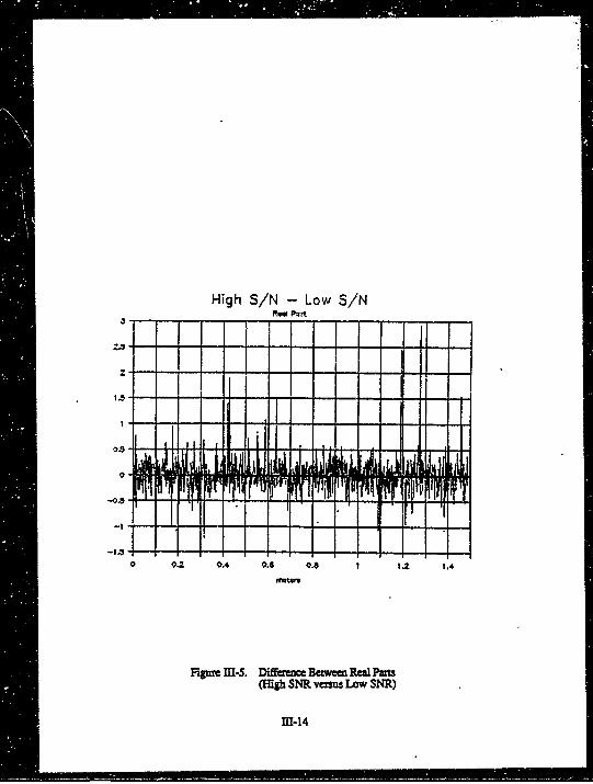
The difference between the high-SNR real component and the low-SNR real
component is shown in Figure 111-5. The phase error spikes are clearly visible.
One of several possible methods for locating phase errors of this type is by
inspecting the derivative of the real (or imaginary) component with respect to the spatial
coordinate. If s(i) represents either the real or the imaginary component, then define the
derivative process
which is a one-sided estimator of the derivative of s(i). A spike in the process s(i) appears
as a double-sided spike in s'(i) [(c. the engineering "derivative" of the continuous-time
Dirac delta function].
rl-ll
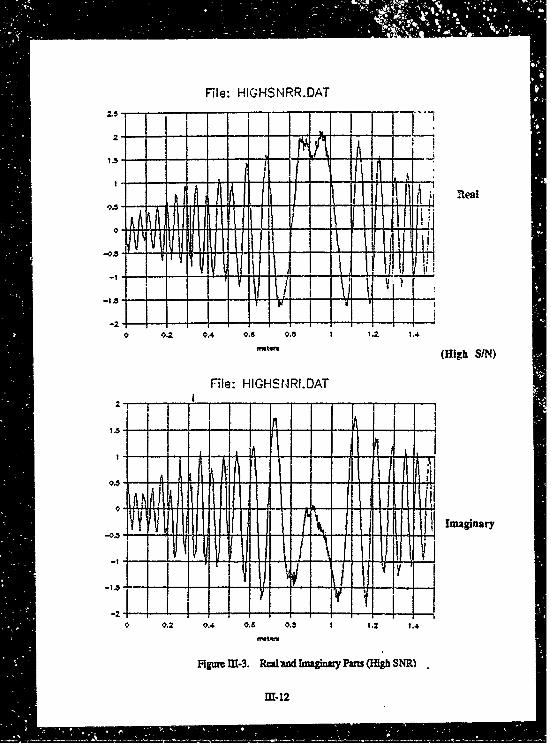
File: HIGHSNRR.DAT
I 1AI
08 I. . .~ 1.2 1.4
Fi=M3.RdtI~gk(High SIN)R
-M01
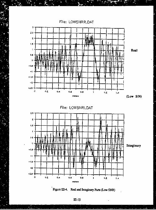
File: LDWENIRR.DAT
~' ~ 2 Real
rxtvj(Low SIN)
File: LOWSNRI.OAT
Ii Il i l1I Imaginary
0 02 4 96 0.8 I 1.2 2.
Figure M1-4. Real ad Itnagiary ?an= (Low SNR)
M1-13
High S/N -Low S/N
0.2 ~ ee 0A 0. 08
3 -~1 ~ MUM
Figure M-.Dfe I-eBtee e a
I:--'- -N essLwSR
1 -M-14
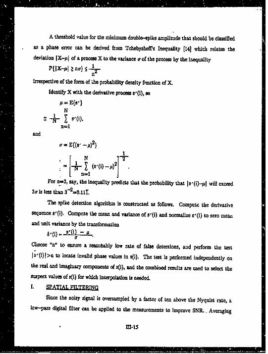
A threshold value for the minimum double-spike amplitude that should be classifiedas a phase error can be derived from Tchebyshef's Inequality [14] which relates thedeviation I X-p I of a process X to the variance u of the process by the Inequality
Pf jX-P1, U ~n'S- 2
irrespective of the form of ;he probability density ftmction of X.
Identify X with the derivative procss s,(i), so
= E{s'}N
n=1and
a= E{(s, _P)2}1[ N1
.=(s3(i) -P)2
For na=3, say, the inequalifty predicts that the probitbility that Is,(i)- Il will exceed
3uis less than 32i=0.11.
The spike detection algorithm is constructed as follows. Compute the derivativesequence s'(i). Compute the mean and variance of s'(i) and normalize s'(i) to zero mean
and unit variance by the transformations'(i) -•
Choose "n" to ensure a reasobtably low rate of false detections, and perform the test"" s '(i)l>n to locate invalid phase values In s(i). The test is performed independently onthe real and imaginazy components of s(1), and the combined results are used to select thesuspect values of s(1) for which interpolation Is needed.
I. •P.AIALfI .TEBISince the noisy signal is oversampled by a factor of ten above the Nyquist rate, a
low-pass digital filter can be applied to the measurements to improve SNR.. Averaging
HI-15
groups of ten adjacent samples is a simple approach to the filtering but distorts the higher
spatial frequency components of the desired signal and has suboptimal noise suppression
characteristics.
A linear-phase filter is required to avoid spatial phase distortion of the measured
signal. A finite impu!se response filter in the spatial domain with cutoff at normalized-_ cut off
frequency vcutof=can be constructed aa follows [15].
We wart a FIR filter of the form
-= a,-1,wherei =0
m F number of coefficients (odd integer), and
a. z f-;Ite coeffic:ents (real).
To ensure linear phase, we define the filter coefficiets -ymmetrically as
cl, i•0, 1, 2, ...q,
whereq- (m-4)/2,
q~ 5
The ideal low-pass filter has tzransfer function of the formf I if V < Ventoe• ]
Hd Y = 0 if v ?• Ucu to• jTaking a discrete Fourier transform to the spatial domain, the filter coefcients are
sin(i " ~Cutoff)S - , i=O, 1,...q.
Gain and phase response plots (not shown) verify that this is a linear phase
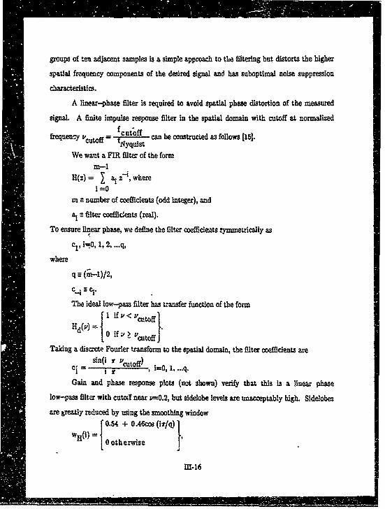
low-pass filter with cutoil near z;-0.2, but sidelobe levels are unacceptably high. Sidelobes
are ,reatly reduced by using the smoothing window' 0.54 + 0.46cos (i7/q)
wHil) jo0 otherwise
M-16

so that
CI cif ' wH(i).
Sidelobe levels of the filter composed of the c1 (Figure M4-6) are about 50 db down.
At f=1/A, the highest spatial frequency that the plane wave spectrum can contain outside
the reactive near-field region, the corresponding normalized frequency is zt-0.1, and the
filter's gain Is down by a factor of 0.92 (about -0.7 db). This level of attenuation will have
negligible effect upon-the near-field data analysis.
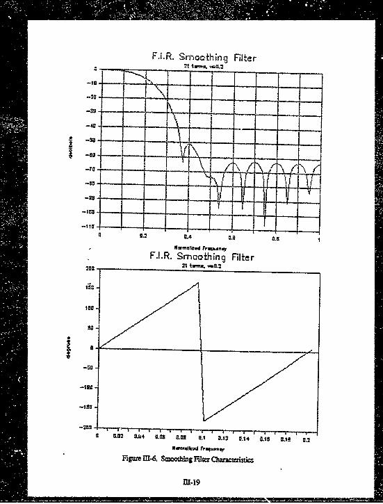
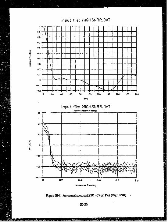
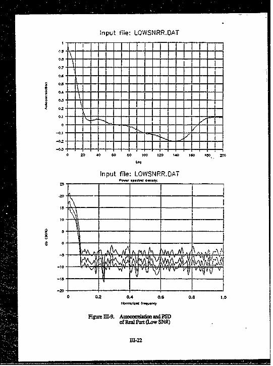
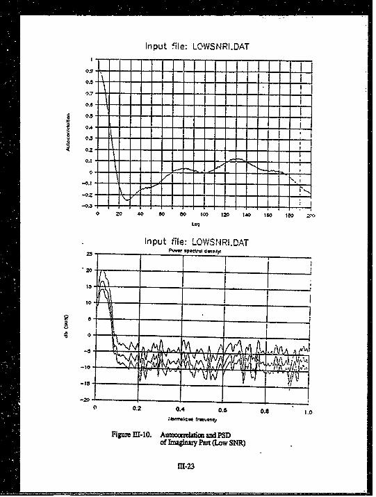
J. POWER SPECTRUM ANALYSIS
Autocorrelation (ACF) and power spectral density (PSD) of the real and imaginary
components of the two scans are shown in Figures MI-7 through 111-10. The smoothing
window bandwidth Is 0 013 Nqst* No differencing of the signals was performed,
although slightly better PSDs might be obtained. Note that the PSDs are down by 20 to
30 db at thi I/A frequency. The noise floor is down 35 db (high-SNR signal) and 20 db
(low-SNR signzl). One may conclude that the measured signals are indeed bandlimited to1/A.-
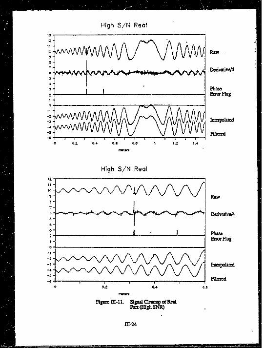
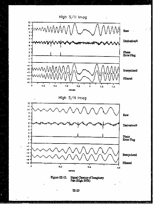
The composite plots in Figures Mn-1I through 11-14 illustrate the effect of the
spike detection, interpolation, and spatial filtering algorithms. The data traces in the
figures, from top to bottom, are
(1) raw data (real or Imaginary),
(2) normalized derivative s'(n),
(3) combined "phase error'; flags from real and imaginary components
using Tchebycheffs Inequality with n=3,
(4) signal after phase errors are replaced by intevpolaed values,
(5) final, filtered signal.
The scales of traces 1, 4, and 5 are identical, while 2 is shown at 0.25 sensitivity.
Each scan (comprising about 1.5 meters) contains 1000 gain-phase sample pairs. For the
1M-17

high S/N scan, 0.3 % of the phwe- snples wom fund hnalid; 2.2 % of the low SIN scan
values were InvAUd.
PSDs of the filtered signals axe shown in Figures M-15 w-d M-16. Note thM the
phas enor correction and laltering have lowered the. noi•e for by ten to fifteen db.
r-1s
F.I.R. Smoothing Filter
•- , I ! --I-7 "I I -...
0 .2 1 .4 0 . I 0 .1SIIK j Vn•D rwmianw1
F.I.R. Smoothing Filter
-led-
-222
i M.02 ,U4 (LS Mae L . 0.12 0.14 ELi 17.13 0.2
Fig= M-6 Smoothing ltctzij= c
1H1-19
:nput file: HiC-HSNRR.DAT
0.-1-9.614 -
OzI
-0.1
Input file: HIGHSNRR.DAT
-toI
0.4 0 it to0
Fiu-M'.Amocomhfmiia and PSM of Real P=x (Mhii SNR)
FI Qut, fi! e: HiGHSHIJ~.OAT
0.7 J . - ~ t J
oz.~ -
-.0.2
0 20 40 so a* V"~ 120 140 1w0 I8 a 0.
Input file: HG-HSN-RI.OAT
-:3
20. _. 0.4 0 _ _0__ __0 _ __ _ __ I__ _
Fig _ _-S _ _m-M~ an_ _ f m~r utOoS
8 1 .21
input file: LOWSNRR.DAT
0*2-- -. _ __
10 ______ 40____ ___0__ to '00 12 14 10 __.
-3 - M A /A MVAA rA1
0 0.2 0.4 0.6 0.8 1.0MormfixW froq¶,.my
Fig=r M1-9. Aumoca1atioa and PSDof Red P= (Low SNR)
M-h22
Input file: LOWSNRI.DAT
0.8*_ _ _
g 0 . 5 ' -
0.2- 4"1
0-- 1 -4I --I- --
0 20 40 60 80 tQ 22 4 10 10 o.
Input file: LQWSINRI.DAT
M-2
High S/NI Real
v ft
Devad
phsEto3a
3V A iroae
A , AW
0 0.2 0.4 0.6 0.0 1 1 .2 1.4
High S/N Real
'2 Ph
0 0.2 0.4 OX
Figurc 11. -i. I=~fx
M1-24 .
High S/'tI irag
-Z bterpolazive
4ee
-6 Phase
0 . 0.4 0.6 e I 2. 1.
H &gh S/ IR)
22-2
Low S,'N Imag
Raw
ii III ag
~j M N\PI\J \VVWIFfiered
~Raw
DeI W
In v W-W 'WInterpoaed
0 0. 0.4 0.6
Figire 1-14. SignalCleaupof1m~ginazyPart (Low SNR)
111-27
Input fe AAHPF1LT.D~aT
10 T
0 1
0 0.2 0.4 0.6 0.6 1.0riomiwzid r~~c
Input fil1e: AHIFILT.DAT
$0-J
0-
-10
0 0.2 0.4 0.6 0.6 to
Figure 11115. PSD of Red1 and bma~iazy P=rtAfte.- Cleanup (RIfi SR
M1-28

Input flie: Aý-RLT.CAT
20
-to
0 0.2 0.4 0.6 0.8 1.0
r4:rmQ1I:v rraueuay9
Input file: ALFIFLT.OAT
-to-
Figure M1-16. PSI) of Reatl aid Imagary PartsAfter Cleanup (O-w SNR)
M-29
CHAPTER riFDESIGN AND CONSTRUCTION OF SCANNER
A. dQF-A
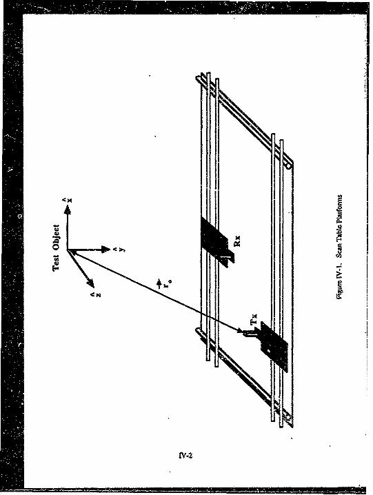
The sca table (Figure IV-1) has two movable carriages, each with one movable
platform. The two platforms are referred to as the TX and RX platforms. Prior to
scanning, the TX and RX platforms start from known initial positions defined by reference
marks on the scan table. The initial positions for the TX and RX platforms are near the
lower-left and upper-left corners of the available scan area, respectively, as viewed from
the operator's position. The stepper motor control software compensates for the offset
between the initial TX and RX positions, so that coordinates for TX probe, RX probe, and
test object are expressed in terms of the same coordinate system.
Optoelectronic sensors are located at the home positions of the platforms. When
the scan table is initialized, and at intervals during scanning, the software moves the
platforms to the home positions and verifies that the stepper motors are still calibrated
(i.e., no steps have been lost). If the software finds that steps were lost, the previous
segment of data i. automatically reacquired.
When near-field antenna measurements are performed, the antenna under test
(AUT) is mounted above the table pointing down, and the receiving probe antenna is
mounted on the ML platform. The TX platform is not used in this mode.
When near-field bistatic RCS measurements are performed, the object under test
(OUT) is mounted above the scanning table, and the transmit and receive probe antennas
are mounted on the TX and RX platforms, respectively.
B. PRBEANENA
The probe antennas are Identical equal-length open--ended sections of X-band
wav4nide or pyramidal horn antennas. Each probe is held in a mounting bracket thai is
bolted to a single mounting hole on its platform. The TX and RX probes are always on the
platforms, as indicated in Figure IV-1.
'V-I
U- •
N ,.3
411
ii .<-
Both platforms are used when performing bistatic RCS measurements; only the RX
platform is used when performing antenna measurements.
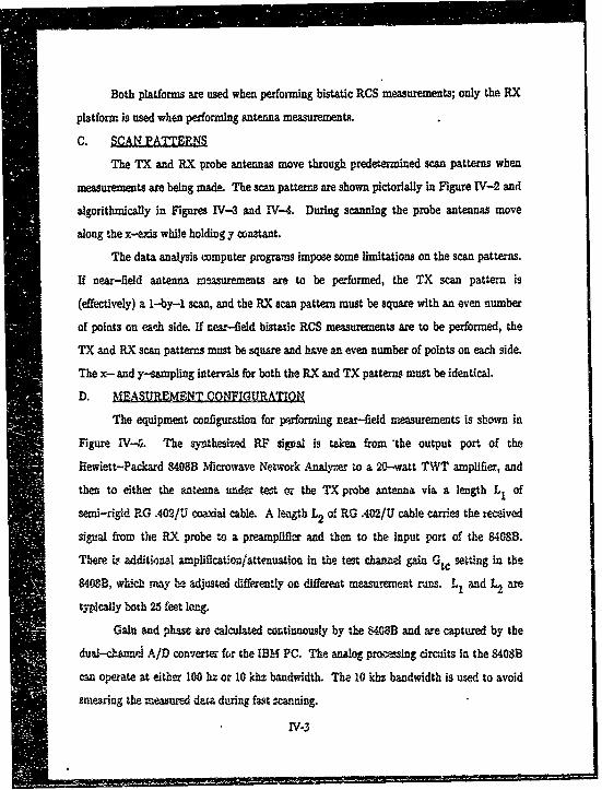
C. SCNPTEN
The TX and RX probe antennas move through predetermined scan patterns when
measurements are being made. The scan patterns are shown pictorially in Figure IV-2 and
algorithmically in Figures IV-3 and PV-4. During scanning the probe antennas move
along the x-exis while holding y constant.
The data analysis computer programs impose some limitations on the scan patterns.
If near-field antenna measurements are to be performed, the TX scan pattern is
(effectively) a 1-by-1 scan, and the RX scan pattern must be square with an even number
of points on eath side. If rear-field bistatic RCS measurements are to be performed, the
TX and RX scan patterns must be square and have an even number of points on each side.
The x- and y-iampling Intervals for both the RX and TX patterns must be identical.D. ME-SUMMFNT CON•FJO%&
"The equipment configuration for performing near-field measurements is shown in
Figure IV-&. The synthesized RF signal is taken from *the output port of the
Hewlett-Packard 8408B Microwave Network Analyzer to a 20-watt TWT amplifier, and
then to either the antenna under test or the TX probe antenna via a length L, of
semi-righid RG .402/U co&axil cable. A length L2 of RG .402/U cable carries the reweived
signal fto the RX probe to a preamplifier and then to the input port of the 8408B.
There -q additional amplification/attenuation in the test channil gain G., setting in the
8408B, which may be adjusted diffexently on different measurement runs. L1 and L2 are
typically both 25 feet long.
Gain and phase are calculated continuously by the q4M8B and are captured by the
dual-channil A/D converter for the IBM PC. The analog processing circuits in the 8408B
can operate at either 100 hz or 10 khz bandwidth. The 10 khz bandwidth is used to avoid
smeming the measured data during fast scanning.
IV-3
-I0 ~ 0
A I_ _ _'
.... • r-"I
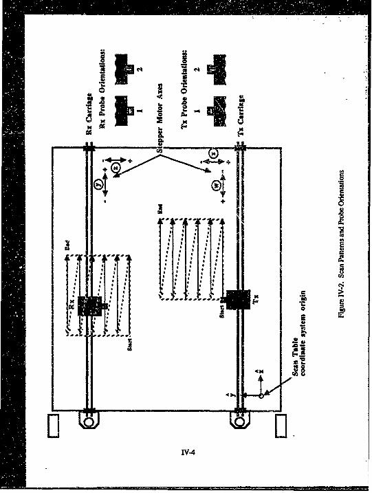
C P$=ed-o for Antenna Measureent ScanningCC NXRXNYX in number of poins along x~y for RX probeC DIRXIYRX - loop indice for RX scanningC XRXORG,YRXORG - lower left corner of RY scan pattern
C XRX.YRX - current coonliinates of RX probeC IRXO a RX probe orientationC DELTXY = sample interval (meters)
C
DO 2O IRXO-1.2
DO 10 IYrX=1,NYRXDO 10 IXRX=lNXRX
XRXX=XRXORG+(XRX-1)*DELTXYYIRX=YRXORG+(IYRX-1)*DELrXY
CALL MOVE(XRXYRIOCALL MEASURE(GAINPHASE)
CALL WRr•(GAINpHASE)10 CONMNUE
PAUSE 'Chang probe orientation now.'20 CONTINUE
STOP Done.'
Fg= IV-3. FORMRAN Code for AntennaMeaee Scan PatMr
iv-5
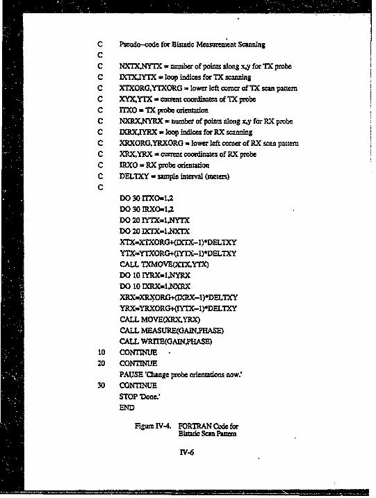
C Pseudo-cod for Bisuxic Measurement ScanningCC DNX MN - number of points along xTy for TX probeC IXTX IY1X - loop indices for TX scanningC XTXORGYTXORG = lower left comer of TX scan patternC XYXYTX = current coordinae of IX probeC rrxo - TX probe orienttionC NXRX,NYRX - number of points along xy for RX probeC IXRXJYRX - loop indices for RX scanningC XRXORGYRXORG = lower left corner of RX scan patternC XRXYRX - current coordinae of RX probeC IRXO = RX probe orientationC DELTXY - sample interval (meters)
CDO 30 rTXO-I,2DO 30 IRXO1I,2DO 20 IY7IXI,NYIXDO 20 IXX=NXTX
X7X=XCrXORG+(DCTX-1)*DELTXYYTX=YTXORG(K=-I)*DELTXYCALL TXMOVE(X Y=X)DO I0 IYRX=INRXDO 10 IXRX=-INXRXXRX-XPRX.ORG+(CXRX-I)*DELTXYYRX-YRXORG+aY -I)*DDELTXYCALL MOVE(XRXYRX)CALL MEASURE(GA•H-ASE)CALL WRrMEGAINYPHASE)
10 CONTINU -
20 CON'TUE
PAUSE 'Chang probe orientations now.'30 CONTINUE
STOP Done.'END
Figur W1-4. FORTRAN Code forBismtic Scan Patern
IV-6

iWaveteki ri nc -I7D5ISIModel~ u ICowiter I
HP'8410 C Gain 50 mv/db Simpson
n RG Scon- W4E el 460
PLL2hase 10 mvldegree LD2LJVarian Tektronix
7A26.4021UG Scope
T T
.x• 4402/11U
Y1Rx eAChannel HP
7046AxY-4 Y2 RecorderChannel
_•Tektronix
7A26
IBM PC CnetComputer (12 bit)
Fig= IV-5. Equipe Confiigrad
IV-7

E. DATA ACQUISITION SYSTEM
Data acquisition is controlled by a computer program that runs on the IBM PC.The program controls the scanning table motors and A/D converter and stores the
measured data to disk.
The conversion time of the 12-bit A/D converter is typically 25 ps. Gain and phaseare sampled simultaneously by dual sample/hold amplifiers and then digitized in succession
by the A/D converter. The measurements are the gain (Vg) and phase (Vý) voltages fromthe network analyzer. The actual gain and phase are computed as G = Vg.gain and
O= V.fo, where 'gain Is a gain calibration factor (20.0 db/volt) and f, is a phasecalibration factor (100.0 degrees/volt) for the 8408B analyzer. The gain and phase are
combined into a complex number and stored in a disk file.
"IV.8
CHAPTER V
COMPARISON OF MEASUREMENTS WITH SOLUTIONS
A. .INTRODUCTION
The far-field RCS that is calculated via near-field RCS measurements may be
checked by comparing it to the far-field RCS predicted by electromagnetic theory. The
conducting sphere and disk are convenient objects for this comparison, since an analytic
solution exists for the sphere and a physical optics solution may be applied to the disk.
Equations for scattering from sphere and disk may be found in Appendices C and D,
respectively. In this chapter we present a quantitative comparison of the far-field RCS
obtained via near-field measurements with the calculated far-field RCS of the conducting
sphere.
Although full bistatic scattering measurements were made on the sphere and the
disk, funding and time limitations precluded our performing the data reduction and
analysis of that data. The results presented here represent scattering from the sphere only.
These near-field measurements were made at 10 Ghz using the experimental setup
described in Chapter III. The target is a precision 6 inch diameter aluminam sphere
mounted above the scanning table. The measurements were made on a 64 by 64 grid of
points with the transmit antenna stationary and directly under the target, so that the
target illumination was essentially
S= 6E( %y.
B. COHRENTJ BACKGROUND-S BTRACTION
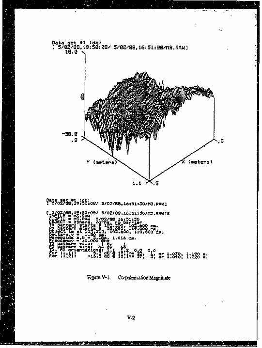
In Figure V-i may be seen the magnitude of the co-polarization component of the
raw data measured by the receiving antenna. The target sphere, located at (xy)
coordinate (1.02,1.02) meters, is above the lower right edge of the plot, corresponding to
the peak amplitude of the raw signal.
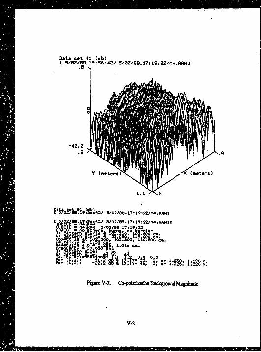
Figure V-2 shows a background plot with all parameters identical to the previous
plot with the exception of the target sphere, which was removed from the test volume.
V-1
Data sot 41 Cdb)
~~ 5/289 se:Stg 5/(meters)0/3.~W
c 3/ qq~l~j~~q/5/02/Ga,1 a51:30/ftM.RM3S
.RAW Z./02/88 16:81.t30=SphereI m .rfAnbare
g Ptter Stai I flvpatt rn a&:Pi
FIguVi. 2opirzicMgid
a u SM"
Data set 91 Cdb)C 5/02/68,19:56:42/ 5/02/99,17: 19:22/M4.RAW]
.. 9
?';017S*"19g42/5/029S.317:±9a22/M4.RAWg3
c ON 42,1 5/0VS9,17sl9&22fl4.ftMbas3/0-/88 17t19:22
at r0 O.O, L.O
1.0.0
Fiur V.2 t op~r~ao Iak~n Mgi
x a toV.3

Although there is no coherent background signature visible In the figure, the raw data are
noticeably cleaner after this background ca is subtracted coherently from it (Figure
V--3). The improvement in signal/noise ratio is even more apparent in Figures V-4 and
V--5, which are contour plots of the imaginary component of the co-polarization before and
after coherent background subtraction, respectively. Similar improvement occurs in the
cross-polarization components.
Coherent background subtraction is performed for all data shown in the figures In
the remainder of this section.
C. DAT[A TAPERING
The first step in the analysis of the raw data is a two-dimensional discrete Fourier
transform (DFT). The signal processing aspects of the data analysis are illustrated by the
effects of several tapering methods that were tried. Figure V-6 shows the magnitude of the
DFT of the co-pularization signal with no tapering; this is equivalent to a rectangular
("boxcar") taper in the continuous domain. The direct scattering from the target shows up
as the large peak in the figure, and probe-to-probe coupling appears at the upper left and
lower right edges of the figure. The side-lobe level due to leakage from the main peak is
about 30 db below the peak.
In Figure V-7 is shown the magnitude of the DFT of the co-polarization signal
after a separable cosine taper of the form 1 + 2 cosM was applied to both the x-axis
and the y-ais. Note that the sidelobe level is better than 40 db down and the
probe-to-probe coupling peak is much more localized, although there is little fine structure
discernible on the peaks.
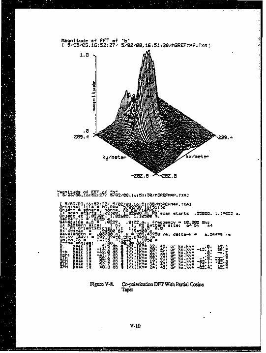
Figure V--8 shows the magnitude of the DFT of the co-polarization signal after a
separable, partial-cosine taper was applied to both axes. This taper consists of a cosine
taper spliced onto a boxcar-type taper, so that the middle half of the data are unaffected
while the first and last quarters of the data set Are tapered. The sidelobe suppression of
this taper "is generally poorer than that of the cosine, but for this data set is
V-4
Data set 91 Cdb)C5/03/88, 5:20:25' /S~g,1:13/1R~I4R
C ~5/02/69, l6s S1'30PR~l4 -RAW 3
up a 5rgjý RAW~~: :a!oi a
x Ottern sze jb
Fig=r V-3. Cojoaiza.io After Backgttmd Submdract
V-5
I heft In r n are
.V.
~b.s 892. 137 1'.33X Cmetarsz)
IW ,: I . 3011ISRERWM4. RAW I
50/ 1 6
251Ijop ttentri
Wavequ~d. a -bI . 1a. I*016 cm.TX pattern Sizes bF ~trn $L :3 6' byFor' -T b IX, Y- , .L :ii .
Figur V-5. Co-=oaito imgriny Pa= AftrcBackgon S=b cun
V-7
Magnitude of FF7 of *bE ,39,32:5 '2991:13'SE'4TA
2.4
299.44
ku/meterx/meter
~ /M?1Pt14.TXAIscan star .1SER'~~ 0,3&e's' can starts .55050, 1.19000 agbloctat 1.5~ M6A SS5uaveu±A a.6 .0 fo 002a,1requency - 10.000 Oh:.*tr Size~ I10 by pa~gttern s±:e: 64 by 64orienntatlol v. 0,0
avelanths - m kc ~41-050 /a, delta-k - 6.54498 /m.KxK (X)- 45_ .rn!9Co IK.
1 ~ 41 or81k 1.1Sth ab K ' * i or kx,scy -1 3.1' 5M.'
r Is~ a * or kx,ky- -1. -6.pek4s Si 6 b XK ,aor kx~ky- 45.8U.. a:k i:i: g3 X Y 'g!E EOr kX:~ -k:" i.
Figure V-6 Co-poWauiao DFr Wuthou Tape
v-8

Maomltude of FFT of *b
209489.4
24/ 1434"N"11 ;ý29,~~ :30/flcEPMi41.TXA3
~~~~ jaý84:1s~ /2/S~i~ 3/R?4T.TXA3
scan stta~z ao~o
&-x , 0 to X Ecan starts .500 1.19000
X, * squmil 10,000 Oh-RX X-scan 6Wave1gn~ th _Q0~A k 4 IC et-k -634B
an1* 1.150 44a rk~yS~l t: XT-~ 4 or kx.kyE : -, :~ ~ ~,Or kX~kyRIPN li El*.: Orr kg~jY k,~,ST DokkKxorX,k
y4
Figui~ V-7. Ci~.o~~iwonDFFWTh aCobinTapca
V-9
flaonitude of FF7, of -b5'V23'GS,16:52:27' 5/92/69, 16:51,:3/MS=REFM14P.TYAI
i.6
269.4 29-
ky/meeter xd/mete~r
5/0V9 16 52:~/0/9I±~S z~/?P~c=4P. TXA2
biect s pherq, hgrmn, no arrirt~~~~Z 4 scnsat '~26r Iscan starts .TZWO. I. :9CC .ZObject at 1. Wj 0 , I ~ .0 a.Way &- -. I am
w Iule ab - R-29, .00- A., f*rquenry - I0.50hz"0X -ter size: i b,' O±R aks iE: M~by'(~p orientail I I r; nsz:5
WAXvs-ien2 6 -- ~oa~~ 4:ne1 /a. delta-k - 6.544Q8 ;M
Xo,Yo.Zo - .14ThN. .U~nP-cbesM:2 1?:: a
0ab '; 42, or kx~ky- .0 *.
L. pea Is, 4.db Y ,* or k;:,kya-t.§mPeak is db K*,c k~yR~~~~h~
-I -1Y -,o xxPH ~ ,d b6X.Y: , or kx k: Sy~PHpek± b Kx *y
9k 4j, or Ix,ky' J-TX;,H Opeak ll. ma b *1a KY , or kxc,kv -s~
Figure V-S. Co-poisrinfion DFr Witb Partia Cosine
V-10
comparable to that produced by the cosine taper. Much more structure is visible on the
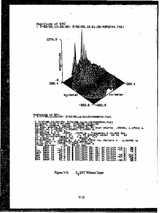
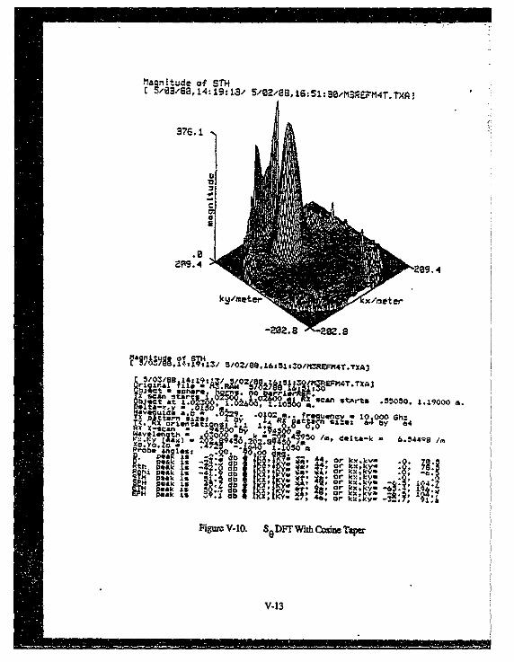
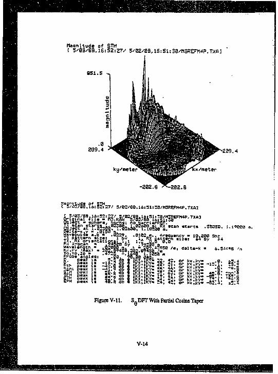
peaks (a common characteristic of this type of taper).A similar judgment may be made based on the calculated scattering matrix.
Figures V-9 through V-1l show the magnitude of Sa calculated using no taper, a cosine
taper, and a partial cosine taper, respectively. The cosine taper has the lowest sidelobe
levels, while the partial cosine taper has higher sidelobes but more derail in the
transformed data. In general, the additional detail makes the partial cosine taper
preferable to the cosine taper.
D. PROBFE-PROBE COUPLING
Figures V-3 and V-8 illustrate the manner in which the measured data aretransformed from a Cartesian coordinate system with units of meters (Figure V--3) to an
angular spectrum with units of reciprocal meters (Figure V-8) in k-spae. The directlycoupled signal from* the transmit probe to the receive probe appear. in the angular
spectrum as a broad peak with incident wavenumbers near the horizon (i.e., Ikz2 c 0) in
angular space.This direct signal can be separated from the desired signal if the desired sigal is not
too close to the direct signal in k-space. Note that (Figure V-8) the probe-probe coupling
appears as a broad peak at the top left edge of the plot and spills over (due to wraparound
in the DFT) to the lower right edge. This broad peak is distinct from, and does not
corrupt, the desired signal in these plots.
Under these conditions, the only detrimental effect of probe-probe coupling is that
it increases the required dynamic range of the receiver.
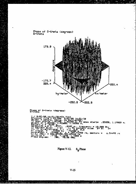
E. REGION O F DEFINI
The region of definition of the reconstructed RCS is limited by the size of the scan
area relative to the apparent angular extent of the object as viewed from the center of the
measurement scan. In general, the actual area of definition is relatively small when viewedin k-space. The reconstructed phase of So shown in FiM re 'V-12 is valid only dyer a small
V-I1
?Iaonltude of STIhE5/03/88,13:20:35/ 5/02/9, 1S:51:30/1l3PEFM4.TXA3
1276.5
209.4 .
5/02.'G8,L&:~lSZO/nKWfFIP4.TXA3
~~~2 ct ~ ~ I -o -n .j0uA*LOct Ct sphere
Sc4, *Can start .55050, 1." a.--ta-x
x~ x an th k-y '94,~ k-~~4gv~ena k 'It;95 / I, delta--6.98/
prao o-±2b ~ j orkxks13NVCd K Ky.
Em k o 1 dlb vX.KY" 4pmt Ido 4 or knk -58.:
Figure V-9. S 6DFrlowzbuTaPcr
V-12
?ianiltude of STH
zgt9. 4 0.
~a~goiP9i131 5'0 2 /SS,L6S51lZ0/fl FM4T.1XA3
Xb sa scan StArt* 50O .90
,gtrng O02a. frLRnc . Ig4og0 Ghg4
WavCI~lanth A6
04 6 _k t4 030 /m, delta-k - .544q9 I
_b ,akx.kv- .0*75
P e a 4 4 ~ C os b * Z k o r N. 9, -a .peek is 48oji: ~ 'j4110ak 12. db 'K . or k, =- *l'A
Fig=~ V-10. SeDFr With Cosioe T&pe
V-13
Placnitude of STI4
25.5
-202r.98 202.9
C 5/02/e8. 16s51:ZZ/KZFMt4P.TXA3
ýi~san stpare, R5!IM ~ S t~ cnsat .552 .ie
Wa'S u±s a.b 6 -- 229, .0102 a.*4-~wc-10.0m8 Gti;TX p2ttorn slxgs I bv 1 RX 88ar 16 6. by 6.4
"IvIlc'ath L I.4 90/, dalta-k - 6.5-=zS /m
Prob, anglon: I
PA -.0 5: do IK, K1 o" r k::Ly kvoeak I~s :-ý K* o __ 'kC
PkIs d .Kx, lKYa .4 r k~ k- ~
Fig=r V-li1. S 0DFr ViM PArtWa =C smT~ap
V-14
Phase of S-theta (degrees)S-thet a
-179.72-09.42294
-M. as 202.8
Phag. of S-theta (dograu.)S-t Lt
/ . 5/e2/6 16lZALZ0,MZ4. TXA)rigi~nai 78I - M.. hA4W 5/02/381:
wav 6vul *. .2!20 .0102 m., irecauencv - 10.0 C+Pfttern 1i~ I b Z RX gat~aý,n ax:t.: 64 b),
R Y A-.can - q 4~
FV' .t I, ur A !M2 S 0Pb
V-15
semicircular region that is approximately
-Z3 meter <k. < 50 m.tei
60 meter-1 < ky < 140 meter-'.
The actual region of validity is blurred due to the sampling geometry and signal "leakage"
between adjacent DFT values- The leakage has been reduced in these plots by applying a
smoothing tqaer before performing the Fourier transforms. The region u validity ippears
in the figure as an area of smoothly-varying phase that is distinct from the phase noise
that covers the remakaer of the k.-ky plane.
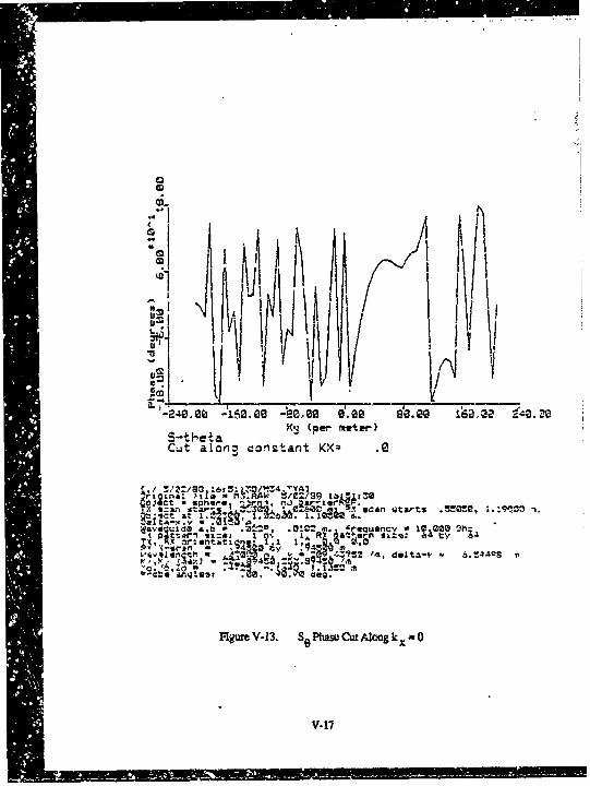
F. CUT ELMS
The region of definitiou appears also in cut plots through the kx-ky plane. A cut
through Figure V-12 along the line kx=O yields the plot shown in Figure V-13. The phase
fanc:ticn ie well-behaved for 60 meter-1 < ky < 140 meter- 1 , while it oscillates rapidly
'nd randomly outside that region.
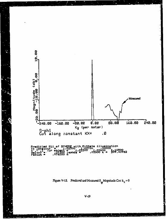
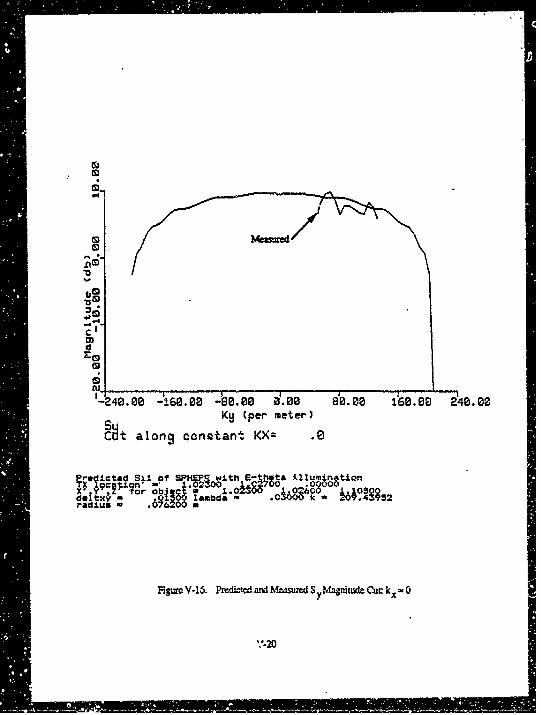
Figures V-14 through V-26 show overlay plots of the predicted and measured Sol
SV SX, and Sy in cuts along the kx andI y axces. A fixed offset of 6 db has been added to
the measured scattering magnitude to facilitate comparison of predictions and measared
data in these plots. This offset, occurring consistently iA all of the measured scattering
dita, is attributed to a calibration inconsistency that time limitations prevent our
-escdving Recall that the region of definition in these plots is approximately
-50 meter7- < k. < 50 meter 1
60 meter-' < ky < 140 mtetii1 .
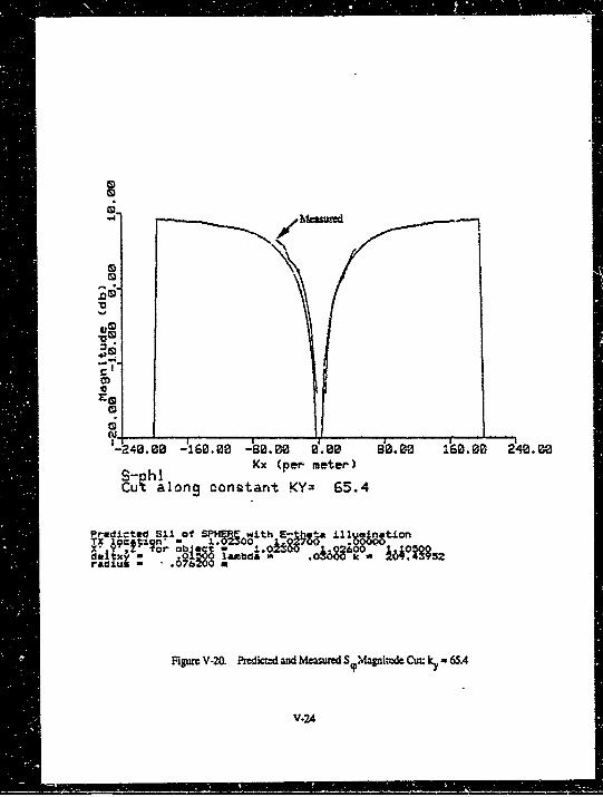
"Figure V-14 show2_ the predicted and neasured magnitude of the function So alocg
a cut kx = 0 mete&-. The deep notch in the predicted magnitudc is a point of phase
ambiguity in this coordinate system representation. Over the region of definition, the
reconstructed mignitude is eszentially flat with about *2 db of residuMl ripple.
Figure V-15 shows the predicted and measured magnitude of the function S V along
a cut kx = 0 mete- 1 . Along this cut, the predicted S 9 is zero except ior an impulee at the
V-16
_29,0015.00 -EC, 00 0.009e 12,a LS-the4Kj (Per maetet)
Cuzt aloln' constan~t KXz .
ts Ata L1d .714 * .Z1, 1 .tel
Y0* -4 Arqec -I-c
y - ,, l* * t t S a d 4 -,?; '
Flom V13. S PiaSO Cut Along k XvO
V-17

Meuuitd\
.4
-
*0
-09
LV02
-240.00 -2160.00 -'89.80.00 d0.00 169. 00 249 .00
S-theta K9 (per meter)Cut along constant i<X= .0
Prollicted 3S.± of Sr* wt E9It l~~EtoTX Y. citign oz3OO~ -
Figure V-14. Aedic~and ±'I=g 1C50C Magninide Cur k X
V-1
Measured
-40,00 -160.00 489.0~00 d.0 d.9d 1'6000 240.00
S-ah1 Ký (per mete-r)Cu alng -. natant KX= .
Pr ite SI fSPH t hot&~ ±il ~tion
FsgwmV-15. Predicm'dand Mesued S (PMagnitude Cu~t kx = 0
V-19
M)
1-240.00 .00 20 .0e 00 YO.9 80 1'60. 0 240.00
KU (per' meter)C~t along constant KX= .0
Pr~dca X.a SPIA with EO;M*t U1Ium~n~ticnx~ictl S of EM w
Taiu .0 008
,!-20
M. Meastuedv.4
'4*
.c1I 40 .0 1 0 0 '0 w d - o e is j c a
o o"JO.Z ,T b.- 31 A 2 k 14 33raiuL
fium-1. rciccdn~emrdSP=Ct~ I-'JVI21

~Megawuu
a.4
'-246.00 -166.6.0 .80.00 '02 8'0.08 160. 00 240.00KB (per meter)
Sch along9 constant KX= .0
FWurcV-18. P-edl-zcdwW.dMua~n.d S y OhmCur k ,- 0
-240.00 -'160.00 4~0.00 0.00 60.00 1,60.00 200
S-theta Kx (per meter)Cut along conetant KY= 65.4
Predictsd S;I of SPHERE with E-thota ±illin~a4ion
TX loettion - 1.02300 jj700 000X, Y*- for obM 1 1. 0 Mr:.t:y .69lg lambda - A83 k- iWM.
F-ig=tV-19. Predicted and Mensuzd S e Maontude Cut ky 65.4
V-23
-7
--- h Kx (p er m et er ")
Cu• along constant KY= 65.4
SPrediLctw S;I of SPI'I_ wit:h E'- ].. il! 0tionrTX 19c1Vqn" - T.02S00 01
d:Idjxy m .01e00 1arbi A680)00k: - 20M52
/-24
. . _ ,.tj w . . . , . .. • . ,.,•• ,• ,... . • • n :.e ,,..,,• • ., - _• :. .-. _ , .. - 2
cI
1240.00 -2160.00 -'80.00 8• 0 80.00 16.8 eeKx (per meter)-- '• Sx
Cut along constant KY- 65.4
Pradicted S11 of SP)¶ 0Ht; E-•.e ±1X•.tkanTX 1ipa•tn wit E-02h00 ill70 , i.00000X .Y 11 fo 17n l;: ', 102•0 lg" O--O0F 100do orxy .0 01402radius .6§200 .
Fig=V-21. Predicted ad Mcawred SMaVnwde Cut w65.4
V-25
.-- '•==i .. 0 -0 J160.0 -S.0 r, |0 00 140 in.0
.4 ln cntn K= 6.
Xll y 9 orral ul -I6000,,,
-- 42
Kxc Cpeirn etetr.C•t aion9 constant Ky= 85.4
SPr.e!ictge S±.i of SPHERE with E-thwta ±11 mnationTX 19C!;i n" ., 1o0. 0 O
Figir•'e V-22.. P~edic•¢d mzd Me•uc Sy Magziot¢ Cu= •: •, 554
V-25
M.
.W-
2t-480 0 -'160.00 -ee. Pa 8'B b'. ea 1166. c '2'4o. aS-thetakx (per ftetei-)
Cut alone9 conatant KY= 65.4
df.x 1 T.4- ±1 16M52c
FigureV-23. R-zdictd and Mca~wcd SePh=seCu ky- 65.4
V.27
-4%
.C4
-. 40.00 -2160.00 438ee 0998.00 1.6 TOS IZ0.0 240. U
S Phi Kx (per meter)Cut al1ilg m-ntant KY.= 65.4
qrilxcr* $ -24 of~~n Mcsur S9 sd-th Cuzý ik 6Pa ya
C-I
LID
LIMd0 a)-8.0 0 ý. 0 ý0 0 ie/9
T 4-8 -1,8 -T.2 .8 Sb5 190 .~6Sx KxO-.0 I.e Sooe
1ancý .~ e.0.or
FigureV.25. Prmdk=-d ad M=e~sr3 Ph= CarY 65.4
V-29
Meawe
Ulm
-240. -16g. 30 Jae. 0 0 do. ~30.0 10. 00 140. 00Kx (per meter)
C& along constant KY= 65.4
Cwcteo S11 of SP 0 thE~j 3 a±i~tOXy irob qt - 1.O2o1M 6c M4.5
lambda .04-6 b0 k
Fig=r V-26. Pftdimeý wW~ Mmveasd S yPhaw sc k 65.
V-30
origin. Th;, reanstuucted functica is ab.,-t -20 db from S&, indicating that
cross-polarization leakage occurred due to antenna gisagnment.
Figure V-.6 shows the predicted and measured magnitude of the function S. along
a cut IC = 0 meter-1. '•-he predicted Sy is acarately .reconstructed with about *2 db of
ripple.
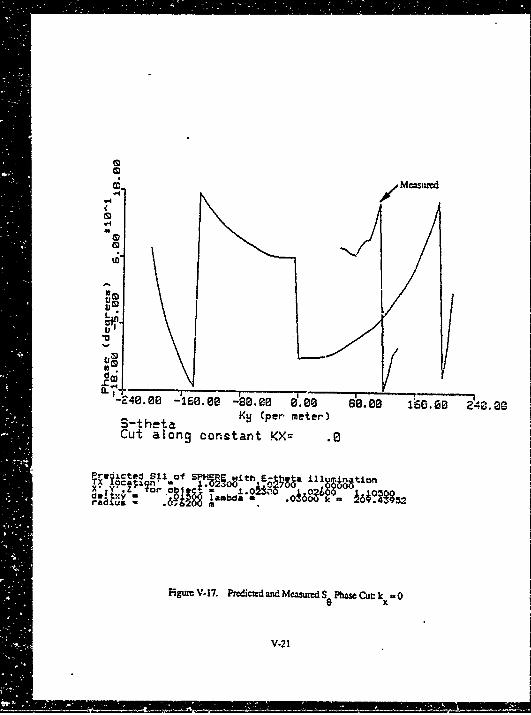
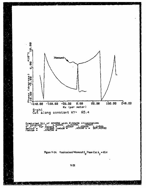
figure V--7 shows the predicted and measured phase of the function S9 along a cut
k. = 0 meLýa1. in these phase cut plots, it is imporant to view only the actual region Gf
definitiop gien above. Over that region, the phase agreement is reasonably good; the
upwyd parabolic tIope to 6he right is discernible.
Fl.ure 'V•18 shows the predicted and measured magritude of the function S. aeong
a ott kx = 0 me~er- 1 . Again, over ih1 region of definition, the reconstructed phase agrees
reasonably re.l with the predicted phase, provided that one takes into account the pha."
w-rap that ocmcur at about l.5 meter-,.
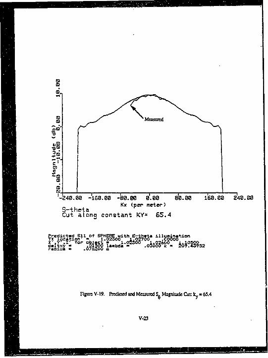
.igure V-19 shows the predicted and measured magnitude of the function SO z'ong
a cu! kr= 6.5.4 meteri-. Along. this cut, where the region of definition is approximately
Ikyl • 50 meter7-, the agreement btween the two plots is excellent, with about 2 db
maximum error.
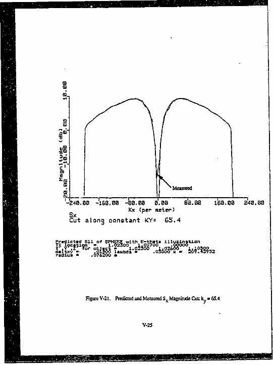
Figuie V-20 shows the predicted sud measured magnitude of the function SP along
a cut kx = 05.4 meteri-. Agremtnt is again quite good, with the saxne offset of 6 db.
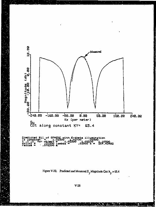
The same may be said of Figures V-21 and V-22 whit show the predicted and measured
magnitude of the functions S. and Sy along the same cut.
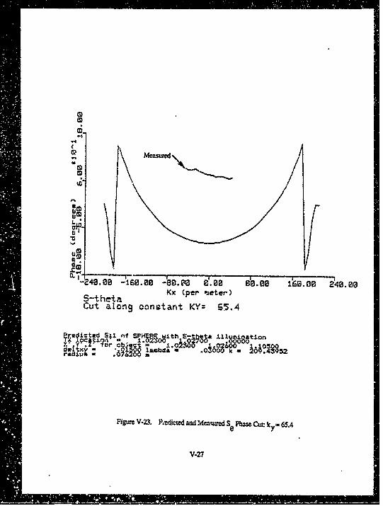
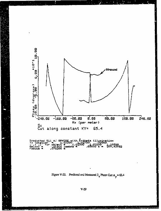
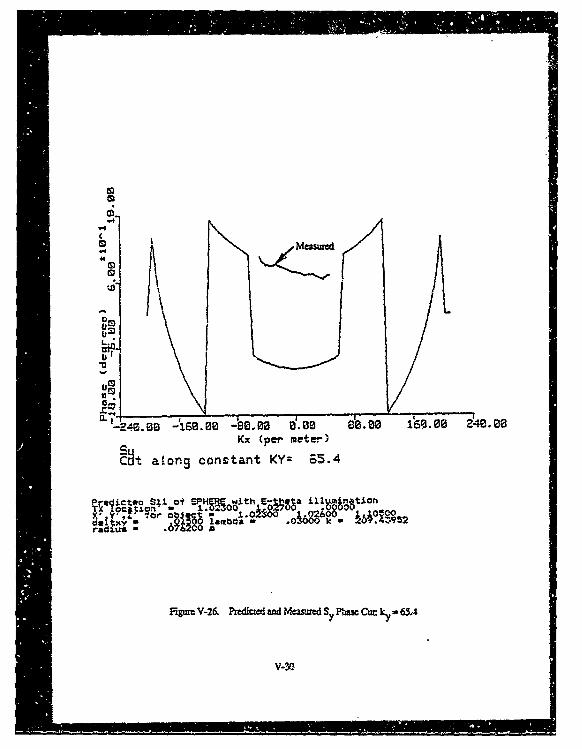
Figures V-2.1 through V-26 si-ow the predicted and measured phases of the
functions SP S , Sx, &ad S y along a cut k,,= 65.4 rreter-I. The measured phase plots
show a linear additive phas2 term wi' h slope of about 0.3 degree/meter;, this term is
pro"bably due to target misalignment. There is in addition b phase inversion of S and
S~which affects the ruer in w:ich thosu two functions change as the orign (kx =
crossed.
V-31

C-. STUMMARY
In this section we presented both predictions and near-field measurements of
tir-field bistatic scattering of the conducting sphere. The key ),nts of the presentation
may b- summartzed as follows:
(1) The magnitude of the measured scattering agrees well with the predicted
scattering within the region of defirion of the k-space reconstruction. The
discrepancy between measurcment and prediction consists of a *2 db peak
ripple superimpo3ed upon a ranstant calibration oftset of 6 db.
(2) Agreenieat of the scattering phase is not as good. This is due primarily to
two effects:
(a) Phase measmtcments are particularly sensitive to antenna axial
alignment perpendicular to the plane of scanning.
(b) "Wra,-around" occurs in the phase of the measured data due to
(fixed) phase offsets in the network analyzer.
(3) Coherent background subtraction is an effective teclin-que for improving
signal-to-noise ratio.
(4) Spatial iltering to remove unwanted scattering from the environment may
be performed in the k-space Fourier transform representation oi the
measured data.
(•) Sidelobes iu the Fouricr-traasformed measurenents are great', -educed by
smoothing the measurements with a smoothing window prior to perbriaing
.he Fourier transforms.
(6) Probe-to-probe couplizg is rPily separated from the desired target
scat .ering itn•orniton n the k-space representation of the measured data.
V-32
CHAPTER VI
DATA REDUCTION INVESTIGATION
A. INTRODUCTION
The existing algokithms 5or computing near-field tatenna patterns and radar cross
sections of objects impose significant computational burdens. In this section we describe
modifications and/or alternatives to the existing algorithms which offer the potential for
reducing t0e number oi computational steps needed to obtain useful near-field
measurement data. The iLvestigations concentrate on three priruary computational
alterratives described in the idGlowiug sections. The following eher computational
aternatives are n.tt considered herm (1) .dptive nonuniform sampling, (2)
non-rectangular lattice (or grid) sample spacing, (3) stai.Rtically reduced number of
near-field data used in tioe far-'ield transform, and (4) derivative data measurei in the
near-field.
Two approaches for reducing the burden of the near-field computations are
considered here. The first approach i, based on writing the equations for computing the
scattering matrix directly in ,ector and matrix notation. The current equations compute
Y'ie scattering matrix in several steps. Each step requires computations and transfers to
data storage which !npose computational burdeas. These burdens can be reduced by using
a direct matrix formulation of the scattering equation In addition, the other alteinatives
for reducing either the amount of meastured near-field data or 'he computations necessary
to determine the scattering matrix are more convenient to work with in terms of the direct
matrix formulations.
The -,emnd approach --k based on expailsions of the near-field functional components
which allow us to imnnose constraints on the near-field functions The constraints can be
based on (1) the desired or expected analytical behavior of the functions, (2) the physics of
ý!,N, measurement environment, or (3) the informatioru content of the data process.
VI-i
In invest!g!%ting thc comput.tlons from a matrix persp ive, we first rewrite the
equations for 'he scatteing mirix in vector matrix notation. Expressed in this form, the
scnttering .zquation is more eftsily Interpreted and adapted to improve the efficiency of
computing the relitionships betwmen the scattering components. Next we relate tho
scattering matrix formulation vith ths vector formulation of the first subsection and
com..are the results.
The c.xpliclt qolution for the scattering matrix 2ll(KL) in terms of the rreasure,4
at array parallels the solution Civen in Chapter II except that thii de-dvatioli solv'-s for
the scattering matrix in teras of the .neasuree data Yector and r rix -pr-esen4ations.
The equarion development is descried in terds of the coLlnnuora Founxr traisform for
exposition convenience. Equivalent results caw be obtained fo, ,he point measurement
computation of the Discrete Fourier transform using the Fast .. urier tranqform.
The bistatic measurement equation Is
-- ~~~o('1' 2)= 0i1k)'Tlk•''0•d
where0 ( =) = týLe vector transpose of f01(K)
k = Scattering (emerging) direction,
= incident (illumLnation) direction,
?I = Pxrex + Pyrey + Ptrez = receiver Prnbe coordinates,
12 = Pxtex + Pytey + Pztez = transmit probe coordinates.
In the laboratory we measure a multidimensional scalar complex array
M(Pxr 39P,PyrP ltytr,t ela discrete points whose components elements ate the measured
values of bo('12)
(PxrPyrPzrr) I {(P,, PyriPz)•), Pzr = constant,
V'1-2
(PxtPytPzt) E {(P, 'PYti'Pzt)}' Pzt = constant,
4r = {1, 2} an index denoting receive probe orientation, and
ft = {1, 2) - an index denoting transmit probe orientation.
In the first step of the solution, we take the inverse Fourier transform with respect
to the respective transmitter and receiver locations f,, t 2 of both sides of the equation.
fbo('1IP I-im fn' f2 i•' 102 t "i - J~"I .10l .
yfr'
e" d 2''fl a2 dl eIII!i -f ,0
= (2r)6 if lo1(i).,T11(,j) .110(f). • •.(-€d!"d
=(2r)6 fI t() -T11 (n-'m)" 10(-mý)
where i. is defined in terms of its wavenumber kxr, kyr, kzr components in the coordinate
system of T11(•,i). Note that 4r and ft are constants in the above equation. We now
write the equation in terms of the •,I argumentsB (i,-I) :(2,)6 01t(K). -T"J 1 ). 410 (1)
whereJJ "ii'f2÷il r dt
B(k,-I) =j bo(flf 2)-e dr1 dr2.
The minus sign of the vector 1 indicates the direction of the incident radiation
relative to the scattering object. In our laboratory measurements the elements of M(.) are
built up by a concatenation of scans by the rece've probe; during each scan we vary Pxr
snd Pyr and hold Pzr' Pxt, Pyt, fr, and 4t constant. If
Nxr = number of discrete values of Px,
Nyr = number of discrete values of Pyr'
Nxt = number of discrete values of PxtI
Nyt = number of discrete values of Pyt'
VI-3
then M(.) consists of 4NtN A matrices, each of which Yoatalws Nx Ny complex scalars.
The factor of 4 comes from 4r= {1,2} and Ct= {1,2}.
The vectors 101(i) and fi0(1) have specific components reflecting their
dependence on the probe orientations (4= {1,2}, t= {1,2}) polarization components (0,0)
of the transmitted and received signals. Next we define two 2x2 matrices UT and Xt
composed of the respective •1(i) and 110(i) vectors In terms of their specific function
arguments {, 4 and 0, thus
t1(,krrl)I kT Z• [..,ot , * .] = [ 01 frl) 10100k ,4 1)]
['•lt•l )1 Ilo (01A42) Ilo0("fr2t) ]
The quantity B(i,-f) is also a function of the probe and poluization arguments so
we define If, a 2x2 matrix with the diagonal terms specified by the respective values of
IT(-) for each of the four vector combinations of the UK (IM) matrices. Using the above
definitions we can write the scattering matrix equation as
(f~•, I) = (2.)6 LZ(J). T (6,,1) Tr(f)t.
If the matrices 1K and IT have rank two, their inverses exist and we can write the
scattering matrix as
TII(ij) = UT U-1..(IL't)1/(21) 6 .
The matrix inverses for the IK and IL4 matrices are
(TK•-I r 10 1 0(k,42) -1 0 1 4)(kl) /A(r)
[-01Ae(,42) '0i (00 )r -I10(k2 0 1 0 (ii 2 ) 1-[-I 0 1 0(1,fti) i01•.Ca', /t)
where A(r) and A(t) are respectively
A(r) I k &r OX ) 0
= 10 0 (k, 4rl) ' 1 0 0 )( ,t 2 )- 110(10,"r1) 1101ok,2)
VI-4
IF 11---
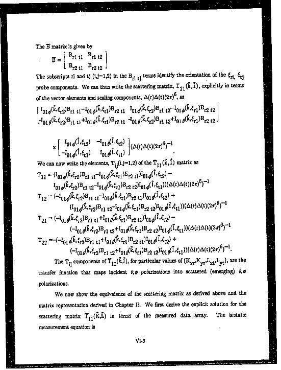
T~he 1; matrix is given by
Br 1Brlt21
The subscripts ri and tj (ij=1,2) in the Bri t terms identify the orientation of the cri, Ctj
probe components. We can then write the scattering matrix, 1 11 (k,1), explicitly in terms
-o~ the vector elements and scaling components, A(r)&1(t)(2jr) , asF Ii~(,42 BritjrIOjO(ý,Crj)Br2 tj l0j6(k',Cr)Br1 tg-l010(i,fr)Br2 t
We can now write the elements, T. .(ij=l,2) of the T (, matrix as
T1 lj(IiCr2)BrI ti IO10i'k4,dF-z2 611)I010(tCO) -
T2= (-IgjO(k,Cr2)BrI tI7o10(L',fri)Br2 td1)IAýZ.,~2) +
(11(,C2BI t210i(ýCri)%r t2)IQj(I,ftj) -~ )~)(r6-
T22 =-(-Iai 6(k, 1,10)Brl t1+lOjiCl~r)Br2 tj~1Ojj 1 'Ct2) +
The Tij components of Tj(,) for particular values of (K ,yxy) are the
transfer function that maps incident 04~ polrzations into scattered (emerging) $,0i
polarizations.
We now show the equivalence of the scattering matrix as derived above and the
matrix representation derived in Chapter 111 We first derive the explicit solution for the
scattering matrix T11(R,fL) in ternms of the measured data array. The bistatic
measurement equation is
VT-5
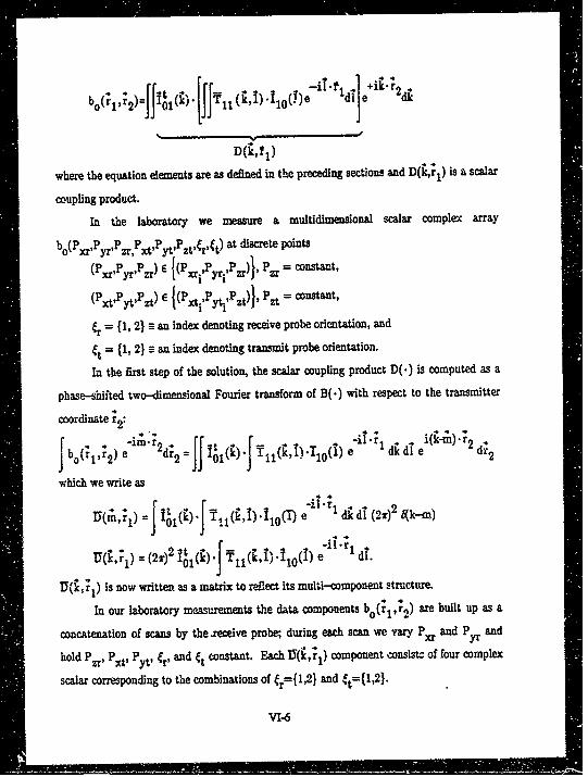
(ktto-) dI e '&-r2
D(i,f1)
where the equation elements are as defined in the preceding sections and D(k,r1 ) is a scalar
coupling product.
In the laboratory we measure a multidimensional scalar complex array
bo(Pxr,PyrP rPxtPytPt,Cr,Ct) at discrete points
(PxrPyrPzr) {(PxriPYri,)}, Pzr = constant,
(Pxt'ytszt) E {(PiPYt ,Pzt)1, PA = constant,
1= {i, 2} a an index denoting receive probe orientation, and
t {1, 2} = an index denoting transmit probe orientation.
In the first step of the solution, the scalar coupling product D(.) is computed as a
phase-shifted two-dimensional Fourier transform of B(.) with respect to the transmitter
coordinate r2:I4 *r * -im- r2 It 1. - m 2
bo(r 1,r 2) e dr2 Jj 0). Y~ ( ;11(•(,1)10 (±) e i dkl ek d
which we write asIU(M,,•) = r f110) .I Tii J•) .•iOM e i•'l- di dT1 (21)2 A(k-m)
1 0i' 1 d.102) ~n
IY(K rl) = (2r)2 I0 T 10). l) "iO( e 1 di .
IY(*,•i) Is now written as a matrix to reflect its multi-component structure.
In our laboratory measurements the data components bo('ii 2) are built up as a
concatenation of scans by the .receive probe; during each scan we vary Pr and Pyr andhold PzrP PPyti ýr, and ýt constant. Each U(k,) component consists of four complex
scalar corresponding to the combinations of f,=(1,2) and ft={1,2}.
VI-6

In the second step of the solution, the scattered spectrumF(i'(1) -- J T11(0'1 "l0(i) e 4'1 -r dI.
is computed from IY(i,:1) and the receive probe response function To,(-) by means of A
simultaneous linear equation solution. From a prior equation 1;(;,'2) is
(t'r,;i) = (2x)2 Tot , I).
Expanding explicitly,
D(i,;1,Cr,Ct) = 101J(,) Fj(k,*r,et) + I01,(•,(r) F,(ilt).
To solve for F(.) we need two equations obtained by measuring D(.) at two different Cr:
D(i,;1,frl,Ct) = o10(1& rl) Fi,1,Ct) + I 01o(krl) Fo(ý,'1,•tD(i,'rl,fr2,ft) = 101•,ýr2) Fdi,*r1,Ct) + 1010(•,fr2) FO(i,;1,Ct)-
ThenF8(i,;I,,Ct) = [D (k',lrl, 1411t)I010(4, ) - D(irl, 1a 42 t)I01(KI, Crl ],&(r)-'
Fkf1,(t) = [D(K,rI,4rl,ft)Io1(k,42) -D(k,r1,i 2 ,ft)Io01(k,r1)JA(r)F
with non-zero determinant
A(r) = I010I(kri)Ioi,#( r42 ) -IO19(,r2)I010('Ird)
For each transmit probe position (Pxd.P c,Pzt) a orientation ft, F(.) is defined over all
valid ;. Note that 1'(.) is not a function of fr A particular realization F(.) is the
scattered spectrum from the object, given a particular position r 1 and orientation Ct of the
transmit probe.
In the third step the vector coupling product is calculated as a two-dimensional
phase-shifted Fourier transform with respect to the transmit probe coordinates. From a
prior equation
F(;, 1r) =J T( TTl ).( 1 0(f) e l d
we define
VI-7
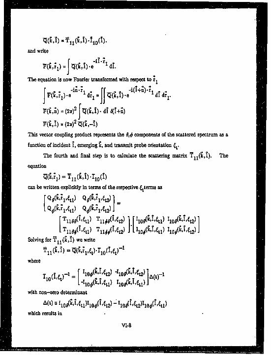
=(,I T11(,1)-41 o(I).
and write
r(ij'd 41 , 1) -•( ~e 4141 dI.
The equation is now Fourier transformed with respect to 1IS(,,1).e-in'r1 +U fr"
(ia) -- (2r)2 Jq(0,1). dl 6(+;)
(,!) -= (2,)2 ,(,-)
This vector coupling product represents the 0,0 components of the scattered spectrum as a
function of incident 1, emerging ý, and transmit probe orientation 4t"The fourth and final step is to calculate the scattering matrix Tjl(i,). The
equation,( r(I,*) = Tn1 (ib ).10(t)
can be written explicitly in terms of the respective Ctterms as
[~~~ ~ ~ C•k l•l ,k•,t2)J
T1100 (1,t 1) T11i0(i,ft2) '10i(kjtl) Iioe(1 ,•4t 2)
Solving for T (11 (i,) we writeT11 (•,) = ZRk,;1,t).rl0(I,Ct)-
where
Tl ,Ct)- -- [ I1o0(i'C't2) 11i0(0-W 2 I A(t -['10A(kltl) II0ALk],tl)](
with non--mo determinantA(t) =- !10•A(,•,tl)I10O(Tft2) -• I109"CtP)100(",Ct)
which results in
VI-8
I II I 1• • . .. .I• • J J•-- '•... .... • IIIlll• •• •

Q (r ,tl Qo(k',1 ,ft2) *Iio(kt2) AIleO"f't2) 1~ )lSt-11
lc C~rtl) Q16(i, 1, t2) J'1-00O ,fCtlt) Ilo•(k,ftl)J "
We can now write the components of Tll(kI) as
T Q0 140,04042)- 990 1tO 140)io(,41)Tl1000•) = oL't)l•••2 At~t • t) Io(,tl
rlle(L Q k,••~t)x÷(~2 - Q 0 140,1040141~t)1180 0() A(t)
T k, -q9(0 ',tl)Ilo#(',•t2) + 401(14,1,0290o4,1t)11000 = - A(t)
=-q Q(,l1tl) lo(8, t2) +Q t(•,, 1 42) lo8(, l4)
The four components of TII(Mi), for particular values of (M,), are the transfer functionthat maps incident 0,0 polarizations into scattered (emerging) 0,0 polarizations.
To compare the vector and above formulations of the scattering equations, it is
necessary to substitute for the respective •, I and U matrices to show the equation in
terms cf the measured Y data set.
We have, from a preceding section,
F(ij,) = (2r)2 q(j,--).
We use a previously defined equation relating U and F to write the T components in terms
of the IU and T matrices, i.e.,U(K,*rl) = (2r)2 Tot (6)"F( r1).
The Fourier transform with respect to r1 and the wavenumber argument 1 isU(;, 1) = (2,r)2 Tot1(f) 0(,•
Thus, we obtainNM•,) = ((2,r)4 T•I(6)).•T(•-I).
Recall that Uo(*1,r2) is defined in terms of U(i, *1) as
o('1;2)= [(,r1) ei dk.J
Taking the Fourier transform of both sides with respect to ;, and ;2 we have
VI-9
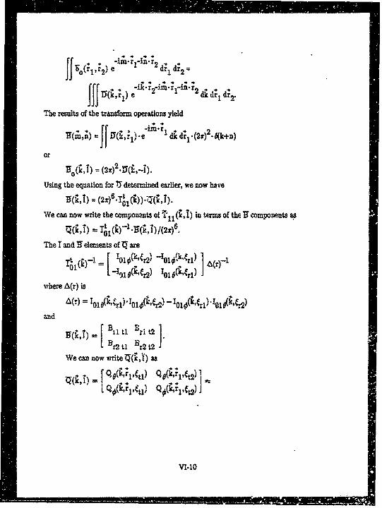
r e4 r
if %( elmrl) drd d
JJJ T(~i~) e "2 d ; d;. d~2.
The results of the transforma operations yield
or
Using the equation for 75 determined earlier, we now have
We can now write the components otfij in tex-s of the If components as
1I(%,) T'i)1f;j/2)
The I and R elements of 'Q are
-491A(W'4 010 ('4rdwhere A(r) is
A(r) =Ii(,~,Ii(k)-li(ir)4i(,~
and
Sil tI Br1 t21
We can now write ZFi ) as
-[Qe(~-'vti) QAl t21
VI-lo
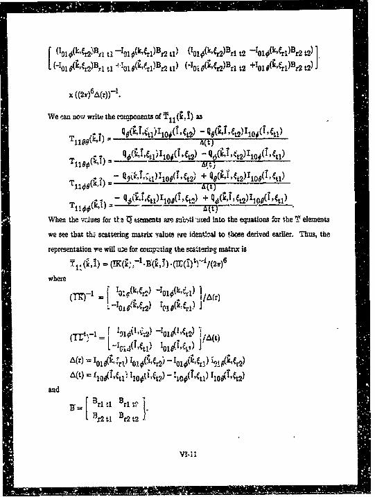
[~ ~ ~~t (T-1k.qj0u (kfri)Br2 t~ (Toi0(k,4 2)Bri t2 -1oi(kýr)B t2(-Iol 8(ý,ri2)Bjl tj -4,30 e(* 41)Br2 tl (-1oi #(ýfr2)Bri t2 +0 (~1B2t).
We.-an. now write the coznnponents of T 1 1 (ij) 33
llook (t)
Tllo(kij) + Q~)1 O ( ,4y)t2Io(lfj .
When the vclues for tf e jq eements we stbb(i 'uted into the equations for the elements
we see that th-z scattering miatrix vfalues -xe ident'cal to those derived earlier. Thus, the
representation re will u;;e for omptzinj the sca~teritiq matrix is
where
-'0 [ f2 'PI{,4 Ioi(itfr) J Ar
(Tr~l f 91 Iýc2) -104G144)~
I -I014(1etl'1 0 ~4 140jA(r) oIo('' k o~~42 -! k~~~4) ~g,
and
13r2-. B r2Q
C. FUNCTIONAL EXPANSION
We consider here a method for reducing the computational and storage burden of
the near-field computations. The baoils for the method is a representation of the measured
data field by a suitable expansion function which is truncated to limit the number of field
function derivatives (to yield a relatively "smooth" estimate of the Licattering matrix) and
which minimizes some specified error function of the estimated scattering matrix. The
equatiops are written in terms of the previously determined values, T,,(ij), of the
scattering matrix and the next value, Tll(K+AZ,I+A1), of the scatterirg matrix to be
determined. As an example, we will consider an estimate for the scattering matrix which
zinimizes the norm, Ni(d). of the waataon definirg the scattering matrix, i.e.
N(d) = I Tll(,i) -I ' -/(2•r)6 m.
The specific ma•rix normalization which might be used need not be specified at this time
for the purposes of this Pxample. The mnimizaticn is subjet to the constraint that in the
reion of each set of estnted values, the scattering mntrix has no derivatives above the
second order. Therefore
T11 (+Ai,I÷+A) =9-.o V j.& 816k + v i.al 8/01](n) T11(r,I)
where V i and V i are thz gradients of the function T,.1(1, ) with respect to K and I and](n) represents the gradient and partial differential operators in the bracketed quantity
being reised to the nth power before operating on the proces functions. The minimization
and constraint conditions are combined using a LaGrange multiplier as shown below:
Q = N(d) + A I(TII(;+Ai,1+Al) -- 4= 0 [V j-Ai 81/ + V I.,& 8/011(n)
The equation for Q is now minimized with respect to A and also T1 1(k,I) for given values
of Aý and Al in order to compute TII(i+Ai,I+AI). The intent of the operations is to
solve for consecutive values of TIj(k+Ai,I+Al) for spacings of Alt and Al which are
greater than those which thight be required if the process constraints were not applied. If
the resultant spacings of AI and Al are greater than those that would be required based on
VI-12

the effective aperture of the scattering object, then we will have reduced the density of data
sampling for the near--eld measurements.
The equations must next be written in terms of the measurement parameters
(TI))-1, (T(l)t)-I and (2r)' and the data variable r(i, 1).
The expan3lon terms in the constraint equation are next written as
h=o 0 / + v r . /81(n) T1(6,I) = t=o [V . o/ + va/aI(•)•(•)-L•tI)•(tt)-'/(2,r)6.
The expansion for n=O yields(IX(i))-1.- E(K, 1).-(M]:c)t)-1/(2r)6.
The expansion for n=1 yields
[V J.b] 0/& + V I.A1 0/011](1 (Tfil.(i ,1).i)-(1)t)-./(2r)6 =
[(-1)(•)-' D -C (.)(•• (1))t1. (V •)- /0 l](f•, )). (f)t)- ]/ 2r+•i)-•.(V t.• 8/& ir(i,)). tt- • +K
The expansion for n=2 yields[V j.4SaI& + V .I /01(2) )/(2) =
[V2j.O .4/A2 + 2-.V i.S V I.Al /olal + V21.&I qp18121.
(TK•(i))-'-90J I•({ -(MI() t)-l. i(2,)6.
Rather than complete the expansion for the second order terms, it is helpful to
cousider the implications of the expansion terms relative to reducing the sampling denmty
of measurements while providing a satisfactory enimate of the scattering matrix. For
example, we might examine the computational and sampling implications of using a
.Deasmrent process which assured that the t (i)/t I and rK'(i)/0t terms would be
sUro.
The final steps are to perform the minimrization with respect to A and the
components of (iC(r)f-.•(•,I).(r(1)t)- in the expansion equations and solve for
'/I-13
. ..... . .. ....1,11 1 IN N . . - •I,. .. .= ,

-TII(•+!,1+AI). The estimated value for TI1 (++A-) is then compared with
the measured value of Tll(i+&], I-c&). If the differen•e between the two values
exceeds a specdfed tolerance value, we have several alternatives depending on the region
over which the funcion -ninimization was performed. If the region is local, the required
spacings of the data samples can be determn~ed adaptively mnd changed as required at each
measurement location. if the minimization region is global then the local error estimates
can be used as a basis for changing the constraint conditions of the algorithm.
VI-14
CHAPTER VII
DEFINITION OF MEASUREMENT LIMITATIONS
A. INTRODUCTIONJ
The purpose of this task was to investigate the limitations, both theoretical and
experimental, of the near-field RCS measurement method. We concentrated on two
topics: (1) data acquisition limitaticns and (2) measurement of wide-angle bistatic RCS.
Investigation into the data acquisition limitations considered the design of the receiver, the
antenna configuration, and the storage requirements. The investigation into wide-angle
bistatic RCS concentrated on the difficulties of performing such a measurement.
Results of this investigation are that, depending upon the frequency of interest,
near-field RCS is practical with current technology for objects ranging in size from small
missiles to B-1 Bombers for monostatic RCS and small-angle bistatic RCS. For
wide-angle bistatic RCS, we concluded that new technology and/or modified near-field
theory is needed. Additionally, application of near-ield RCS for large objects at
frequencies above 1 gigahertz is dependent upon the development of large array antennas
appropriate for near-field.
B. DATA ACOUIsr10 LIMITATIONS
Investigations into the data acquisition limitations covered the topics of receiver
design, antenna requirements, and data storage requirements. This investigation
demonstrates that near-field RCS is possible for a wide class of problems with current
technology and that, with the advancement of new technology, it has the potential to be
applicable for many classes of RCS measurement configurations. In this section, only
monostatic and small-angle bistatic RCS is considered.
1. ReevrDsg
A potential design for the receiver in the near-field measurement method is
shown in Figure VII-l. The receiver shown is a synchronous detector and is similar to
receivers used on typical radar systems. This type of receiver is proposed because of its
V11-1
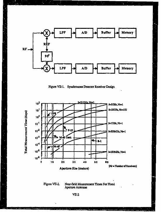
Fiur VII-1 SydrAIuDe r B uffer Memory
F.Gr~.
-'1:2i;
102 10l 20 30I 40511 0IS0
10-2-

ability to rapidly measure the real and imaginary parts of the received signal The real
part of the RF signal is obtained by multiplying the PF signal by a reference signal from
the local osclla"or and low-pass filtering the result. The Imaginary part is obtained by
multiplying the RF signal by the qusdrature of the reference signal and filtering as before.
These signals are then converted to digital form and stored.
In most cLaes, data storage will be the slowest function in the receiver. However, If a
buffer is devised to switch between several storage devices, one could realize a system
which is limited by the A/D conversion and the settling time of the low-pass filter. In
most practical eaues, the A/D conversion time will be the limiting factor on speed If one Is
willing to use a wide-band low-pass filter and accept the increased noise that will be
associated with the wide bandwidth. Conversion times of under one microsecond for 12 bit
A/D conversion are common.
Figure VII-2 shows the measurement time required to make near-field RCS
measurements assuming that the only limitation Is the sampling time for the A/D
conversion. In this example an army antenna with A/2 spacing is used, the A/D conversion
time is 0.1 microsecond, and the time to move the transmit probe Is assumed negligible.
This graph shows that for practical frequencies and for targets as large &a the B-1 bomber,
A/D conversion times are not a limitation with near-field mensurements given enough
receivers. The main limitation of this configuration, however, is the design of the array
antenna and receiver system, and the cost of such a system. Arrays with 106 to 107 array
elements and 102 to 103 receivers will be required at higher frequencies.
2. fla g=
Data storage requirements are extremely large for many practical
,easurement configurations. Figure VII-3 shows tOe data volume generated assuming
conventional sampling techniques and no data compression. The large amounts of data
that must be stored required some kind of data compression to make near-field RCS
practical for large scattering objects at high frequencies. Several techniques for reducing
V11.3
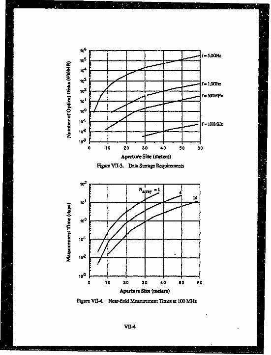
o 100
S 105
104 1 0 3 4 0
1012
10-1 f- 0%&
. 10-2 1
0 0 20 30 40 60 so
ApertUfe SIMe (meters)
Fiig='114 Near-f3d DeamSurmg euetimes 10m z
1021.
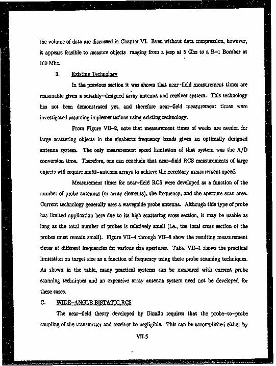
the volume of data are discussed in Chapter VI. Even without data compression, however,
it appears feasible to measure objects ranging from a jeep at 5 Ghz to a B-1 Bomber at
100 Mhz.3. Fdtn eloo
In the previous section it was shown that near-field measurement times are
reasonable given a suitably-designed array antenna and receiver system. This technology
has not been demonstrated yet, and therefore near-field measurement times were
investigated assuming implementations using exdsting technology.
From Figure VII-2, note that measurement times of weeks are needed for
large scattering objects in the gigahertz frequency bands given an optimally designed
antenna system. The only measurement speed limitation of that system was the A/D
conversion time. Therefore, one can conclude that near-field RCS measurements of large
objects will require multi-antenna arrays to achieve the necessary measurement speed.
Measurement times for near-field RCS were developed as a function of the
number of probe antennas (or array elements), the frequency, and the aperture scan area.
Current technology generally uses a waveguide probe antenna. Although this type of probe
has limited application here due to its high scattering cross section, it may be usable as
long as the total number of probes is relatively small (i.e., the total cross section ot the
probes must remain small). Figure VII-4 through VII-8 show the resulting measurement
times at different frequencies for various size apertures. Tabi%. VI-1 shows the practical
limitation on target size as a function of frequency using these probe scanning techniques.
As shown in the table, many practical systems can be measured with current probe
scanning techniques and an expensive array antenna system need not be developed for
these cases.
C. AT!-ANGLD BISTLTC RCS
The near-field theory developed by Dinallo requires that the probe-to-probe
coupling of the transmitter and receiver be negligible. This can be accomplished either by
VII-5
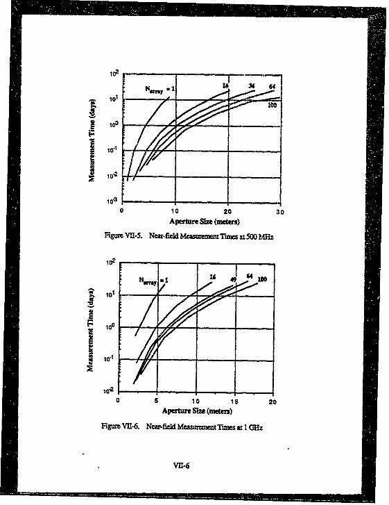
- 101
! 100
10*1
10-
10-30 10 20 ;0
Apertur Size (meter)
Fig=u VIl-S. Nma-field Measurezmnt Thues at 500 ?Af
S101
S 100 1
S10-1--
10'2
0 5 1,0 i's 20Apertmr Size (meter)
Figur VH.-6. Nea-field Measuemet Thme at IGMz
VUI-6
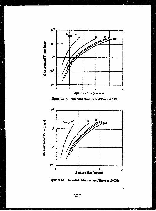
i=- - --
S101 "
~- 00 - -
10.1--4
0 1 2 3 4 SAperture Size (meters)
Figuz VII.7. Near-field Meaurmmn Tzmes at 5 Giz
101
N. 100 4 4 0.101601
Apetur Size (meters)
Figurt VIT-8. Neur-field Mesrmenct Tume at 100Hz
V31-.7
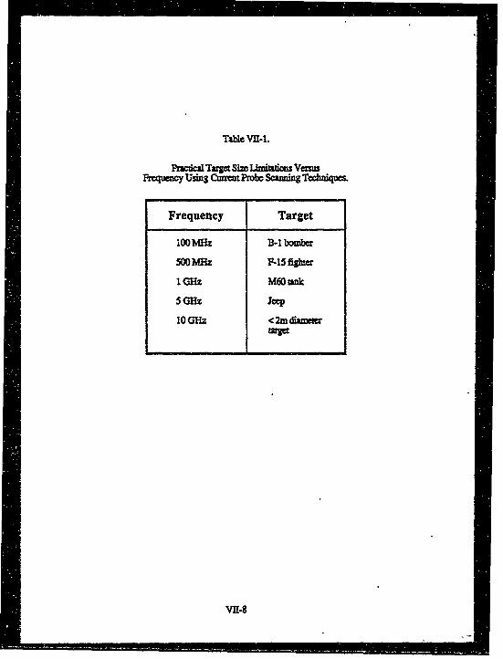
Taue Vu-1.
PactiToggaSizr~Limiiaiou Ve=~aFreque=7c Using uCrntProbc Scanning Tchbnique&.
Frequency Target
1OO!bah B3-i bomber
500MHz F-15 fighte
10M M60unk
10MH <2mdiamea
target

using probes with minimal mutual coupling or measurement techniques such as time
gating, FM modulation of the background (range filtering), k-space filtering (angular
filtering), and so forth. Each of these experimental techniques has its limitations. The
problem that arises is that there will always be potential geometric orientations for which
angular, range, or time filtering alone cannot distinguish between the received signals from
the scatterer and the transmit probe antenna. This problem might be solved by using two
or more of these techniques in tandem. Additional development of the theory of near-field
RCS measurement may also be fruitful. Wide-angle bistatic RCS is conceptually feasible,
but has yet to be demonstrated. Further investigation into using multiple filtering
techniques and/or additional theoretical development need to be performed.D. CONCLUSIONS
Thzu brief investigation has shown that near-field monostatic and small-angle
bistatic RCS measurements are practical for some interesting classes of problems using
current technology. It also shows the need to develop both large array antenna systems
and inexpensive multi-channel receivers. The need for array antennas, and thus
multi-channel receiving, increases with increasing target size and frequency. Data storage
problems also increase with increasing target size and frequency.
The data quantity reduction techniques discased in Chapter V have the potential
of relaidng the constraints for both the data storage and the complexity of the array
antenna by requiring fewer data samples, and therefore requiring fewer array elements.
VII-9
CHAPTER VIII
CONCLUSIONSA. INTRODUCTION
This final report presents the technical work performed by BDM for the Rome .%"
Development Center to Perform laboratory measurements and anzlyss to vnlidate a Wlanar
near-field RCS measurement technique.
The major issues of the technical effort are discussed in the p,=,]ous chapers of thl-
report. The probe corrected near-field theory is well-developed and is directly applcable
to the planar measmuement configuration. Software to implement the theory has been
developed. Near-fielo measurements were obtained with a low-cost computer-a-utrolled
scanning table designed and constructed in the BDM Laboratory. Agreement betwebn
measurements and prvdictions was excellent. We have identified several approaches to
reducing the quantity of data required for near-field RCS measurements, and hav'.
identified some of the limitations of the method.
Although we do not see any fundamental obstacles to implementing this R0S9
measurement technique on a larger scale, our recent work nas given us insight into the typr
of development needed to bring this concept to fruitiou. While building on the mature
near-field antenna measurement technology, planar near-field RCS measurement itself is
obviously not a matu-o technology. BDM is not at a point to design turn-key systems
implementinE this technology, although we have been leaders in developing and validating
the mathematics and experimental protocols for there measurements.
We do feel, however, that this Is a very promising avenue for near-field
RCS measurement. It shows promise of addressing several important issues of RCS
measurement:
(1) measuring RCS of low-observable objects,
(2) measuring monostatic and blstatic RCS,
(3) providing a secure faciiify for RCS measurement,
VIII-I

(4-- increased accuracy, and
(5) increased repeatability.
In the following sections we discuss eow technolo a we that need further
development. Specific arw of planar near-field RCS technology are disussed in the terms
of topic problem areas and tentative solutions. EnvironmezW factors are also noted where
appropr:ate.
B. B&Lcn- ME+ $UR•MENTr REOIUIBEMETS
There is currently a credibility gap that must be surmounted. Although the
.neoretiral basis for -onverting near-field RC• to far-field RCS is firm, there has been no
large-sc.le demonstration thet mear-field RCS data will yidd valid, believable far-field
RCS for realistic military ta-gets., it is necessary to establish analytical bases for relating
onventional far-field RCS measurements and near--field RCS meaaurements, identify
limitations of both far-field and near-field RCS meazurments, and investigate ths extent
to which the statistical car.erxa•ica of faW-field and near--ld daza are complementary.
There will b- szowp difficuWt! a enc-mutered in meabvring low-observabie RCS, since,
as in conventional far-Seld ranges, the RCS may be comparable to the background
scattering levels in the system. It is neceesary to identify mechanisms for dealing optimally
with low signal/noise measurement eavironments.
The actual requirements for RCS data quantity and precision are not clear. While
very accurate RCS from many angles is desirable, what is actually acceptable? There is a
need for realistic RCS requirements assessments based upon system specifications and
mission requirements.
The analysis of near-field RCS data has moderate computational complexity.
Studies are needed to identify trade-off elements, precision, and computational complexity
and apply a systems view of the problem to determine computational trade-offs.
VIII-2
C. THEORETICAL BASIS
Tne theoretical basis for near-field RCS measurements needs expanding. Among
the effects that need additional investigation are multiple interactions between probes and
objects, ways of reducing the computational burden, effects of undersampling the data
field, maximum entropy constraints to reduce what would be redundant information In a
noise-frea environment, algorithm modifications to compute parameters of estimated
statistical distributions directly for RCS or antenna patterns, and more effective probe
antenna designs and patterns.
D. CALIDBATION
Fxisting RF technology is generally adequate to support this RCS measurement
technique. Care must be taken in stable design of signal sources, feeds, and receivers. The
mechanical and electrical design of the antennas and feds will require ingenuity.
Calibration of such a near-field RCS measurement facility would probably require built-in
calibration loops in the RF paths to allow adaptive self-test and recalibration during data
runs. Implications cf such self-test loops, and the possibility of using created white (or
other suitably defined) spatial and frequency noise sources and out-of-band techniques to
check calibration In real time, should be investigated.
E. MEASURING THE NECESSARY DATA
The two key problems for this near-field measurement approach are the amount of
data that must be measured, and the time that will be requi.red to make the measurements.
There is no fundamental obstacle to recording the necessary data, but it calls for clever
measurement system design and data processing algorithms.
The measured near-field data will be voluminous. Ways are needed to reduce the
amount of data required, and to efficiently store the data once they are measured. Possible
paths to pursue are to achieve data density reductions by alternative computation and
analysis algorithms; data coding algorithms to reduce data volume for Ucquisition, storage,
and processing; trade-offs between data precision, storage requirements, and analysis
VMI-3

accuracy; uew algorithms (eigenstructure, analytic and series functions, and orthogonal
expansions) for reducing sampling density; determining what can be done numerically to
utilize magnituie-only or phae-only measurements; use of error-ree versus
non-error-fEm, data comprersion; use of densely--packed antenna a&rays; and investigation
tf various higa-densty digital data storage media including optical disk and holographic
storar B
Other avenues of inv--tigation include fMlly-automated measurements systems,
computer-contro!led data collection and probe and target positioning with process quality
feedback, time-division and frequency-division multiplex antenna and feed systems,
fast-response serve control systems for probe antenia positioning, existing laser metrology
systems for cosed-4oop control of antenna position, multiple transmit and receive channels
with broad-band intermediate frequency strips to allow high-speed I-Q measurements,
parallel computationally-specific dedicated processors, and combined data measurement
and analog computation.
The various RF coupling paths between measurements system and object must be
analyzed as part of the error analysis. Signal-to-noise limitations must be evaluated,
particularly in light of low-observable targets, broad IF bandwidths in receivers, and
system noise figure. Other signal-to-noise issues Include using multiple coherent data
measurenmts, background scatter reduction, coherent or incoherent background
subtrdction and suppression, absorption and signature techniques, effects of multiple
reflections, explicit time gating and Implicit gating using synthetic spectra and data
signatures, environmental changes and deviations from Ideal, and factor analysis.
Part of that investigation would be to evaluate the level of specular and diffuse
reflections that may be present from both object and background, and possibly create
mediflied •1gorithbmstalloied respectively to emphasize or reject specular and diffuse
reflections via a feed-back loop, using resuts to isolate undesired components of the
background.
VM1-4

Obtaining the necessary metrology accuracy is not a trivial problem, but is well
within the state of the art. Tools to be used here include laser interferometry', closed loop
control, real-time RF frequency and phase error measurement and adaptive correction, and
phase locking techniques. Timing errors can be minimized by referring all measurements
to a master clock to correct the time refemces of data as required.
It is necessary to evaluate reproducibility of measurement conditions.
Reproducibility is impacted by environmental effects, equipment drift, structural stability,
target stability, and aging, and might be measured in terms of pattern distr.butions and
statistical confidence intervals.
Effects of non-ideal measurement components (eag., amplifiers, mixers) must be
evaluated. One approach is to exercise and modify algorithms as required to examine data
behavior given non-ideal components, including error analyses, simulation, and
experiments to evaluate effects of component variability.
Possible methods of alleviating undesired effects of probe characteristics include
using broad-band, lot mutual coupling, variable polarization, active nonlinear elements.
Adequate polarization and geometry control may allow simplifications in the data
processing algorithms; this will require detailed antenna analysis and design and feed
systems using PIN diode switching and compensating elements.
Environmental noise components might be isolated and compensated for by
measuring and assigning data signatures to various environmental and measurement
elements and demodulating the undesired signatures in real time. Environmental
interference might also be reduced by using out-of-band data from known targets to
isolate environmental interference on a real-time basis.
Approaches to reducing data computational burden include using canonic
simplifications based on alternative measurement ani analysis algorithms, and
simultaneous measurement, computation, and analysis using buffered computations and
direct transform algorithms.
VIII-5
Data collection monitoring and quality control call for automated operations and
on-line factor analysis to determine data error sensitivity. The need for Identifying
unusual measurement problems during data acquisition suggests that one should create an
evolving data pattern generated incrementally as measurement data are obtained, so that
algorithms can detect divergence from the emerging pattern.F. DAAAAYI
The relations between Input and output data quantity and quality, and numerical
effects in the data analysis algorithms, need additional Investigation. Possible approaches
are to employ a 64-bit (or longer) word-length computer to simulate a variable word
length computer and thus determine the numerical sensitivity of the algorithms and
optimize the algorithms for minimum sensitivity; investigate dynamic range limitations
due to numerical considerations of using large Fast Fourier Transforms (FFTs); and
possible use of phase-only data. Simulations are needed to help determine error relations
between data inputs and outputs. Data analysis time and resources could be reduced by
using dedicated hardware FF1s and processors.
Additional paths to reducing computational complexity include using the physical
situation's constraints (both target and environment), using mathematical structure
constraints, adding other consualnts on information content, matching the information
content of the channel betwe-e, measurements and canonic results, factor analysis, and
various operations research techuiques (including linear programming).
Other poWible data and algorithm modifications include using blank data cells
(under sampling), truncation (blanking), zero Interpolation, blanking interpoWlation, various
simplifications and alternatives to the axsting near-field theory, solving dual/analog
problems, identiWying relations between simplification and useful outputs, computing
pattern statistics rather than RCS patterns, and using object and algorithm functional
symmetry.
VM-6
G. OPERATIONAL CONSIDERATIONS
We emphasize again that it is not clear what RCS data are really needed for
existing aircraft and missiles. It would be a noteworthy capability simply to be able to
measure monostatic RCS at, smy, one degree intervals for angles within *30 degrees of the
horizon, but it is not clear whether missi, effectiveness would be truly enhanced by such
detailed knowledge. Perhaps it would be more useful to be able to state that the maximum
RCS over a specified solid angle is less than - with probability V. The range of angles and
the angular resolution of the data have major technical (measurement time and data
volume) and economic (time and cost) impact. As aids to baselining this measurement
approach, time and data volume could be estimated for specific measurement scenarios,
given the angular range and resolution needed.
The absolute RCS accuracy required for mission evaluation has a major impact
upon how much data are needed, how long It takes to measure the data, and what kind of
algorithms are used to process and display the data. Acceptable and desirable
measurement accuracy constraints for mission scenarios must be established.
The mission scenario elements together impose stringent requirements upon the
measurement system. As part of identifying true measurement needs, a system level
evaluation of mission and operations use of RCS data is needed, to determine feasible costs
(time, capital, and staff), and to perform trade-off analyses and simulations.
VMI-7

REFERENCES
1. Hewlett-Packard 8408B System Manual, P/N 08408-90009, August 1982.2. Yaghjian, A.D., "Approximate Formulas for the Far Field and Gain of Open-Ended
Rectangular Waveguide", IEEE Trans. Ant. Prop., Vol AP-32, No. 4., April 1984.3. M. Born & E. Wolf, Princinles of Optics. Pergamon Press, 1965, Appendix III.4. Stutzman & Thiele, Antenna Theory and Desie, Wiley, 1981, page 16.5. Kerns D.M., Plane-Wave Scattering Matrix Theory of Antennas and
AJnna-Antenna Interactions, National Bureau of Standards Monograph 162, June
1981, page 62.6. C.A. Balanis, Antenna Theorv. Analysis and D , Harper & Row, 1982.7. Yaghjian, A.D., "An Overview of Near-Field Antenna Measurements,"
IEEE Trans. Ant. Prop., Vol. AP--4, No. 1, January 1986.8. Yaghjian, A.D., "Overview...", p. 37.9. Joy, E.B., and Paris, D.T., "Spatial Sampling and Filtering in .Near-Field
Measurements," IEEE Trans. Ant. Prop., Vol. AP-20, No. 3, May 1972.10. Newell, A.C., Planar Near-Field Measurements, June 1985 (unpublished).11. Kerns, D.M., NBS Monograph 162, p. 73.12. Oppenhelm, A.V., and Shafer, R.W., Digital SiZnal Processinb, Prentice-Hall, 1975.13. J.S. Bendat and A.G. Piersol, MeAsurement and Analysis of Random Data. Wiley &
Sons, 1966.14. Papo.lis, A., Probability. Random Variables. and Stochastic Processes,
McGraw-Hill, 1965.15. Natarajan, N.A., Discrete-Time Signals and Systems, Reston Publishing Co., Inc.,
Reston, VA, 1983.16. Dinallo, M.A., "Extension of Plane-Wave Scattering-Matrix Theory of
Antenun-Antenna Interactions to Three Antennas: A Near-Field RadarCross-Section Concept," Proc. Antenna Applications Symposium, University ofIllinois, September 1984.
17. Dinallo, 1984, eq (18).18. Papoulis, A., The FoUrier Intesa and it AnoiLats McGraw-Hill, 1962.19. Stratton, Electromagnetic Theory, McGra-Hhl, 1941, pp. %3 tn 573.
R-1
APPENDIX A
COORDINATE SYSTEMS
A. COORDINATE SYSTEMS
There are two coordinate systems (Figure A-i) to deal with in performing
near-field measurements: the scan table coordinate system (S') and the antenna
coordinate system (S). In the context of bistatic RCS measurements, the antenna
coordinate system is referred to as the test object coordinate system
The scan table coordinate system is the "laboratory" coordinate frame in which
measurements are taken, while the antenna coordinate system is the natural coordinate
frame for the antenna or object under test. Both are right-handed coordinate systems.
The scan table coordinate ,ystem is defined with horizontal x'-y" plane and
z'-axis upwards. The x-axis corresponds to movement of a platform only, while the
y'-axis corresponds to movement of a carriage along with its platform.
The origin of the scan table coordinate system is at the center of the aperture of the
TX probe antenna when the TX. platform is at its initial ("home") position. The
horizontal position of the origin coincides with the TX probe antenna mounting hole in the
TX platform, while the height of the origin above laboratory floor level depends upon the
height of the TX probe antenna that is installed.
The origin of the antenna coordinate system S is placed at some convenient
reference point on the AUT. If ; is the representation in S, of a vector from the origin
of S, to the origin of S, then a vector *r expressed in S' transforms to S as
; = ( -®r ),
where
o x + y oyr 1 001
Y= o 0-1 010 0-1 j
rrx + ry&s + r2 .ý, and
A-1
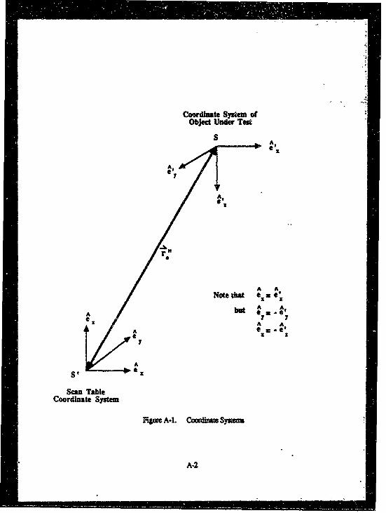
OjCt Under 'TOWt
A,*10
A,
0
A ANote tat e x e
A A,
AAe z z
A
Scan TableCoordinate Systm
F4=u~ A-1. Comiuma~ Sysmmn
A-2

If the unit direction vector A is expressed in spherical coordinates as (,,) then
its negative (-A ) is written as (r,r - Or+ +).
If the unit direction vector is expressed in spherical coordinates In S as (r#,O,),
then it is expressed in S' as A" = (r',9',4'), where
r, re" =•r-9
,= .
If the unit direction vector A is exprssed in spherical coordinates in S as (r,8,0),
then its negative (-A) expressed inS" is-A = (r',Is', where
l= r
&, =-(a+ •).
The above relations can be verified by inspection of the coordinate systems
involved. We require that
r>O
S" is used to describe the probe antenna TX and RX characteristics since these
functions do not depend on a probe's location in S'.
C. ILLUM1MATING PLANE WAVE
The target is illuminated by a plane wave with polarization A, (j1-•=O) that is
effectively emitted from coordinates (xiyjzj) in S, toward the target centered at known
coordinates (x6,yNz) In S'. Define a unit vector *, in S, in the direction (x*-Xi, Y6-yil
"ZP-Zj). The vector "1 is known, since ;i Is a unit wave-vector from the far-field
illumination direction (if TX probe is scanning), or (xjyjzj) is the TX probe position and
ri can be calcudated'(if the TX probe is stationary).
A-4
The propagation vector kfis expressed as
k~i q~k
k~1 =rq1k
or
=- cd-l(ril)
i= tan-1 (il'1,l)
where
k a 2r/A.
We also know, or will specify arbitrarily, the polarization of the illuminating plane
wave. If the TX probe is scanning, we select the polarization(s) EB or Eý for a particular
simulation. If the TX probe is a stationary standard gab. horn pointed at the object, we
will orient the horn so that the object Is on-ads and the E-plane of the horn is either
vertical or horizontal In S,, so that the transmitted polarization is either purely E' or
purely Eý.
If the polarization is known In the basis set
then the spherical components of the polarization are
EI = EisinOlcoso 1 + Ellin01 slino 1 + Ek.is 1
Ek = EIcos01cos• 1 + E; 1coS01sivO1 - E%.sinn1
EýI = -Eisnol + EBicoe 1 .
If the polarization is known In the basis set
then the Cartesian components of polarization are
m = E;isin 1coI + Eicc061COsO - E~lsino1
-Ei = Ei0 1sin$1 ln0 + Eclcesin 1l + EýIco0S#
A-5
El= E' 1cOs91 - E' sin91 ,
and E; must be selected to ensure that •i.i-fO. Thus i can be expressed in either
Cartesian or spherical coordinates using the above transformation equations.
The propagation vector is expressed in S via the transformationskx = +k l
_ ~k,l• =-k;ilor
O1= r-O
, = --4i.
The polarization vector is expressed in S via the transformationsExl = +%,I
Eyl = -E•I
E•l = -E;Ior
Erl = +E;i
Ef 1 = -E•IE01 = -Ei.
Therefore we can express the inlcident wave-vector and polarization (i) in either
Cartesian or spherical components in S, which is the coordinate system of the target.
D. SCATE D PLANE WAVE
The target scatters the illuminating plane wave Into plane waves in various
directions. In order to evaluate the scattering, we select a particular scattering direction
based upon where the observer is in the far-field.
Consider a plane wave that Is rcattered toward the known coordinates (xyiz) In
S'. Define a unit vector '-• in S" In the direction (xj-x6,yj-y6,q--z). The propagation
A-6
vector k is expressed as
k;2 = 72k
or
= k0= -1(.2
di cos '(ri2)
where k B 2r/A.
If scattering in a known direction is desired rather than scattering toward a knowncoordinate, then q (expressed in S') is the scattering direction and (xyp,) need not be
known.
The propagation vector 2 is expressed in S via the transformations
ky2 =--ýk2 = -,A2
or
r2 ri
E. SCATTERING CALCULATION
At this point we know the incident k-vector (i1)' the incident polariztion (i),and the scattering k-vector (k2), all expressed in S, so we can compute the polarization
vector (t2) of the far-field scattered plane wave (Figure A-2) by mean of an analytic ornumerical model of the scattering object. The usual range-dependent phase factor can be
ingored.
A-7
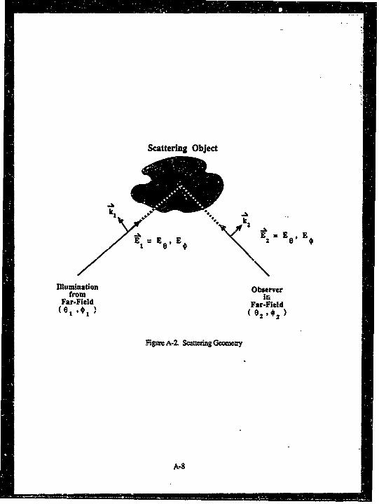
Scattering Object
kk
E Ea EE 0 = ,E 2 9
Ullumination Observerfrom ir
Far-Field Far-Field(e1 '*1 ) (0 2 ,s 2 )
Rpnm~A-2. Scattering Geometry
A-8
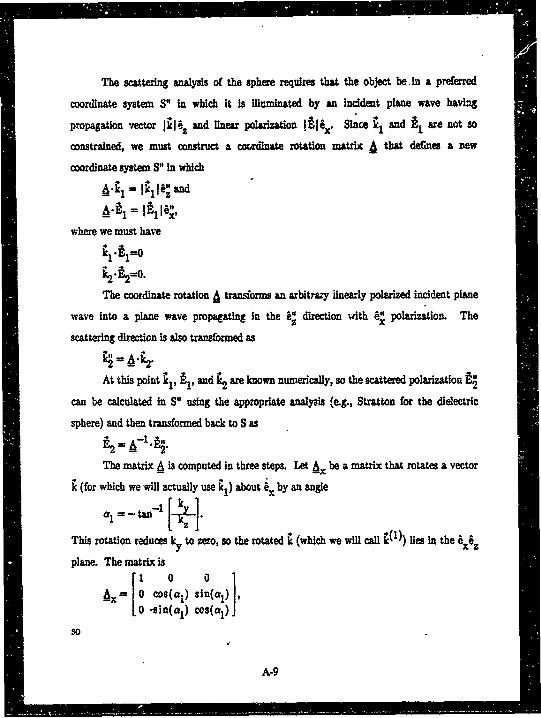
The scattering analysis of the sphere requirm that the object be In a preferred
coordinate system S" in which It is Illuminated by an incident plane wave having
propagation vector jkilz and linear polarization Ibi x . Since and A, are not so
constrained, we must construct a coordinate rotation matrix A that defines a Dew
coordinate system S" In which
' I = I ixl,where we must have
k 2=O.The coordinate rotation A transforms an arbitrary iinearly polarized incident plane
wave into a plane wave propagating In the direction Aith 6. polarization. The
scattering direction is also tranformed as
At this point il, Al, and k are known numerically, so the scattered polarization t
can be calculated in S" using the appropriate analysis (e.g., Stratton for the dielectric
sphere) and then transformed back to S as
The matrix A is computed in three steps. Let A. be a matrix that rotates a vector
S (for which we will actually use ;,) about e: by an angle
a, - tan-1 -_V _J.z zJ
This rotation reduces ky to zero, so the rotated k (which we will call (1)) lies in the 6A
plane. The matrix is
r1 0 0x 0= cos(al) sin(al)
LU -sin(a1) cos Jso
A-9
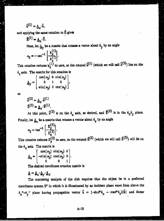
.-
ad applying the same rotation to . gives
Next, let A y be a matrix that rotates a r-ector about 6Y by an angle
This rotation reduces k(l) to zero, so the rotated •(I) (which we will call lies on the
ez axis. The matrix for this rotation is
rcos(a2) 0 sin(a2)
AY 0 1 0L-sn(a,) 0 cos(a,).
soi,(2 ) A xs -i ( ')k(2) ___x.0().
At this point, j(2) is on the ez axis, as desired, and A(2) is in the yx~y Plane.
Finally, let Az be a matrix that rotates a vector about ez by an angler p()
o3 =-&1 [--t•
This rotation reduces EM to zero, so the rotated E(2) (which we will call E(3)) will lie on
the 6. axis. The matrix iscos(03) sin(83) 01
AZ= -sin(a3) cos(%ý) 0].0 0 1
The desired coordinate rotation matrix isA_ = Az.Ay-Ax.
The scattering analysis of the disk requires that the object be in a preferred
coordinate system S" in which it is illuminated by an incident plane wave from above the
61"-4y " plane having propagation vector i = (-,sin'"6x - c "Oz)il and lnear
A-10
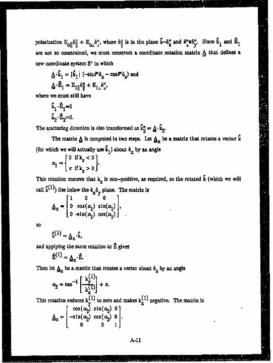
polarization E011oj + , where ZI Is in the plane 1"e- and i'=8" Since j1 and El
are not so constrained, we must construct a coordinate rotation matrix A that defines a
new coordinate system S" in which
All= EIlI + --a ) and=E .+ .
where we must still havek"1*91 =0
The scattering direction is ý w transformed as 4 .2.
The matrix A 1z computed in two steps. Let x be a matrix that rotates a vector
(for which we will actually use lc) about 6. by an angle
21=1°0 ifkz <0r fkz > 0
This rotation ensures that kz is non-positive, as required, so the rotated k (which we will
call •(1)) lies below the 6.6y plane. The matrix Is0 01
x= 0 cos(a1) sin(a)l- 0 -sin(a1) cos(a 1 )
soK(1) = Ax.K'
and applying the same rotation to 9 givesk(l) = _A.-L..
Then let _z be a matrix that rotas a vector about 6z by an angle
r [k( +
This rotation reduces k(l) to zero and makes k(l) negative. The matrix is[ cos(, sn(,2) 01
-z= -sin(a2) cos(a2) 0O.
-0 0 1]
A-11
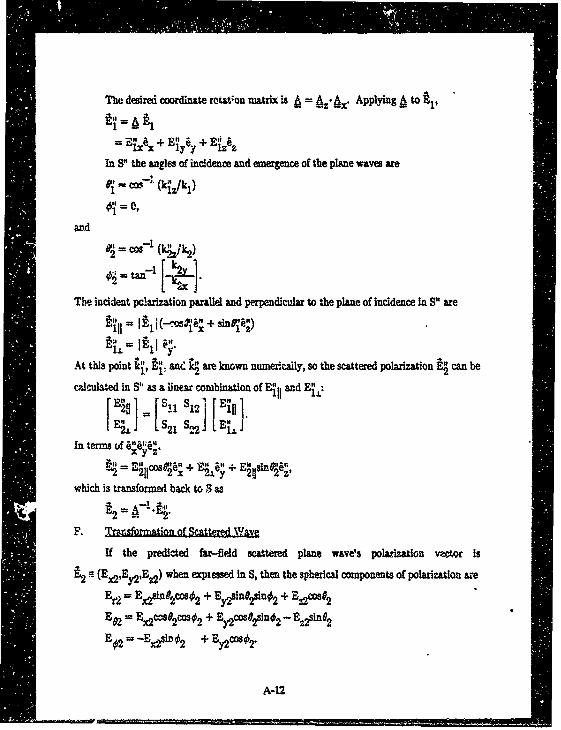
The desired coordinate rotat;on matrix A = i .s A. Applying A to
= ex + Y+ EzzIn S" the angles of incidenes and emergence of the plane waves are
--_- co (k 2z/kl)
and
11 = co'- (k&1/)
=tan•1 ["LJThe incident pclaxization parallel and perpendicular to the plane of incidence in S" are
•.1= I~j-I(-"•+sin ;-)
At this point a, .: and are known numerically, so the scattered polarization E• can be
calculated in S" as a linear combination of Eland E
EF-•L LS21 S2.22 E.L
In terms ufe'" .
61-2" = ~ O + "L;+ Esnwhich is transformed back to S as
S•~2 = C A--'-
F. Musformation of Scatered Wave
If the predicted fa-field scattered plane wave's polarization vctor is
L=_(E.,,Ey2,Ea) when expressed in S, then the spherical components of polarization are
E = E•i•=Acos 2 + Eyin 2s"2 2 + EBzIM 2
E0 = E2dcose2cosO 2 + Ey2cose2sink2 - E%2n92
02= "-EsiD02 + Eyg2CSO'"
A-12
If the calculated polarization in spherical coordinates is
when expressed In S, then the Cartes•,a components are
Ex = EOsn 2cw2 + B.02.OS9co 2 - B-slnO
E2 = Ee 02 + E2osln2 + F20=0
E2 = Er~w 2 - E•sin 2.
The polarization vector is expressed in S, via the transformations%2 =+Ex2
Ey2 ýy 2
%2= AE2
or
E-r2 = +Er2
= -E.E•2 = -E
By means of the above equations, the scattered wave-vector (•) and polarization
(•) can be expressed in S' using eith Crter sa or spherical components.
The far-field scattered electric field is given by A and ', which can be expressed
in term of S or S'. It is probably best to stay In S, which is the natural coordinate system
for the scattering object.
A-13

AA
90
FigmtB-1.ave~4d OpnFdvdu&vmu
B-2fIfl~
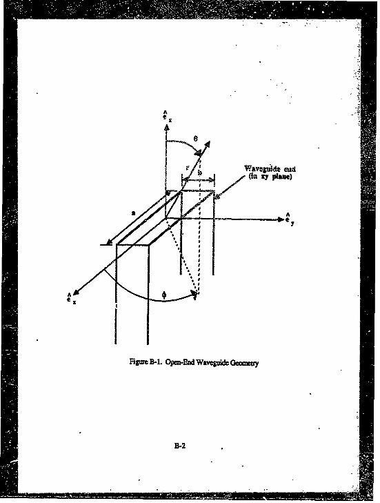
AA
90
FigmtB-1.ave~4d OpnFdvdu&vmu
B-2fIfl~
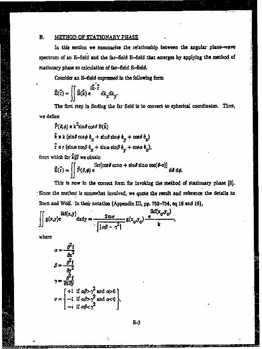
B. METHOD OF STATIONARY PHASE
In this section we summarize the relationship between the angular plane-wave
spectrum of an B--field and the far-field E-field that emerges by applying the method of
stationary phase to calculation of far-field E-field.
Consider an B-field expressed In the following form
2(; =, e dk~dk,.) j
The first rtep in finding the far field Is to convert to spherical coordinates. Thus,
we define
r. k2sin~cosOB(i)
••k (sin x + " sW4 i Y+ coo$1Z)
r a r On&os p ij- SWi + cosa$ z).
izurn which far ji we obtain
W(•) -' ji N ) e lkrcTse Cosa + sin# sina Co("-)] d d4.
Thie is now in the correct form for Invoking the method of stationary phase [3].
Since the mdeh is somewhat involved, we quote the result and refemnce the details to
Born and Wolf. In their notation (Appendix MI, pp. 753-754, eq 16 and 19),
r k(X,y) Ikf* 0,y0IIg(X,y)e dxd[Y 2nrw g(x0,yd
where
i 2f
dzfW
+- if oft> and o>0I
~-1 if< 7OIýýadC
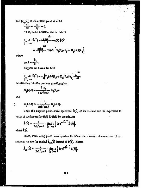
and (xoYo) Is the critical point at which
-M =Df .0.Thus, in our notation, the far field Is -
l•imt N; "2xke
2xke
where
Cos$- k-•--.
Suppose we have a far field1icr
I mi t b(r) -au Ege y mlr l'
Substituting into the previous equation gives
B ,) ,2xk2ccofE0•
andIn
Thus the anguiz plane-wave spenm A(M) of an E-F-leld can be expressed in
terms of the known far-fed F.-feld by the relatio
2*co9 n..[Ie .
where K1•.Later, when using plane wave spectra to define the transmit characristic of an
antenna, we use the symbol (, ) instead of •). Henc
10' 2-AcosD Inl-.. e ~ rJ
B-4
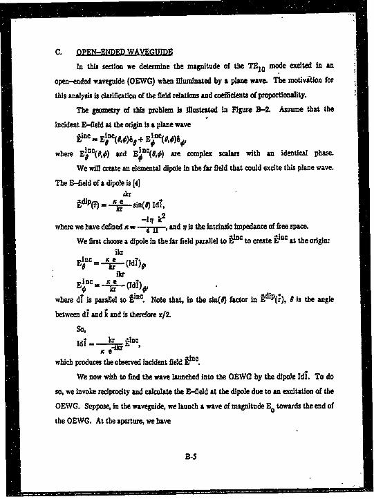
C. OPEN-ENDED WAVEGUIDE
In this section we determine the magnitude of the TEh mode excited In an
open-ended wavegulde (OEWG) when illuminated by a plane wave. The motivation for
this analysis is clarification of the field relations and coefficients of proportionality.
The geometry of this problem Is illustrated In Figure B-2. Assume that the
Incident E-field at the origin is a plane wave
LI C M InC Inc.#B (0,)0A+ EA (0,O),eInc(# ) incr
where E8( ,€) and E# C(1,0) are complex scalars with an Identical phase.
We will create an elemental dipole in the far field that could excite this plane wave.
The E-field of a dipole is [4],kr
AdP = e sin(r) IdT,-1 q k2
where we have defined x - - 4 =, and ,i is the intrinsic Impedance of free space.
We first choose a dipole in the far field parallel to linC to crate VuiC at the origin:ihaInc 1C
Ez = U-- (Id?)pi kr
where dt Is parallel to •n. Note that, in the in() factor In diP(), 0 is the angle
between dI and i and is therefore 4/2.
So,
Idi lckr jnc
which produces the observed incident field fpc
We now wish to find the wave launched into the OEWG by the dipole Md. To do
so, we invoke reciprocity and calculate the B-field at the dipole due to an excitation of the
OEWG. Suppose, in the wavegulde, we launch a wave of magnitude Eo towards the end of
the O -WG. At the aperture, we have
B-5
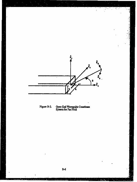
AA
A A
Ax
Fig=r B-7- Open-End Wzvcgtf* Coordi=zSyasorefFvFledd
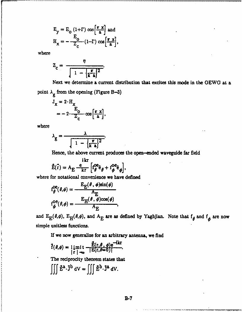
Ey = Eo (1+r) cos [rr] andHx = --E .(l r) x i]
where
17ZC
Next we determine a current distribution that excites this mode in the OEWG at a
point A from the opening (Figure B-3)Jx = 2- Hx
-2---Ec. COS r- x,
where
Ag A
ga
Hence, the above current produces the open-ended waveguide far field
ikr
where for notational convenience we have defined
foepEH( 8, E )cos(i )
AE
and EE(0,0), FM(#0,), and AE are as defined by Yaghjian. Note that f0 and fo are now
simple unitless functions.
If we now generalize for an arbitrary antenna, we find•(0,•) = imi t •,,•e
I I-The reciprocity theorem states thatJJJ t". b dV = J Abja dV.
3-7
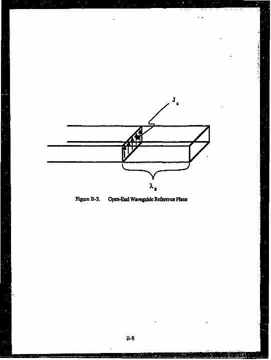
FigureB-3. Open-Ed WkveguidmvR mfetcePl
B-8

In this instance the two cases (a) and (b) are:
(a) the current sheet in the OEWG excites the far field, and
(b) the small dipo!e in the far field excites the TEN mode in the
OEWG.
Now, the mode excited by the plane wave in the OEWG at a distance A inside the
open end is
Ey = bocos(-a-)
where bo is unknown. Invoking reciprocity, we find
j=- 2. BO.-cos[rLaxj.vJa=-2-•gc " a[-] y,
&kr
jb -Idl,
-. e -ie r [Einc6e + Einc6]
and
Eb -bo cosr X &1
The left-hand side of the reciprocity equation above becomesikr
fffa.jbV =A ir ~e~ + ~ f6 kr W ic., i nc- AE f oe + foeinnce
while the right-hand side becomes
jf•bja dV =fb/2 "a/2 bc xi -2Eo rX x d]_'-12 fa 2 loco L-FJ Y-c-c' r - aL j• 64 dr/• r+a/2
0-2b0E° b a2 aXI dx dy.- J ii/2 cosJ-!
B-9
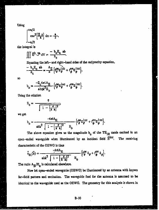
Using
C0a2 r x] T'
Ja-a/2
the integral isH Lb.a dV -- - bOEO ab
Equating the left- and right-hand sides of the reciprocity equation,
-boEo ab AE f incEZ-- Ite jine + oLI c
so-Zc4riAE nc+foeFnI
Using the relation
F1
we get"-4 ziAE tfoe~inc + foeE lnc}bo = i2,• fT ,0 $ 0 .
abl 1-aJ E0
The above equation gives us the magnitude bo of the TEl0 mode excited in an
open-ended waveguide when Illuminated by an incident field ilnc The receiving
characteristic of the OEWG is thus
30()= -7
abk2 I y jT{iJ 0
The ratio AE/Eo is calculated elsewhere.
Now let open-ended wavegulde (OEWG) be illuminated by an &ntenma with known
far-field pattern and excitation. The wavegulde feed for the antenna is assumed to be
identical to the waveguide used as the OEWG. The geometry for this analysis Is shown In
B-10

Figure B-4. Note that the source antenna is placed in the unprimed coordinate system,
and the OEWG probe is in the primed system. We define
ao = excitation in waveguide of known antenna, and
bo = excitation in OEWG.
Both ao and bo are defined at a distance A from the origin of the respective coordinate
systems.
In the coordinate system 0 (that of the antenna under test), the far-field E-field of
the antenna is
M r( ) = ao [EJ0 ,O))& + E 4)(8,4))& + 0 .er] "k'
where EP(eA) and EPA(,4) are known functions, ao is the excitation, and angles 0 and 4)
are related to the propagation vector k by
and
It has been shown that E(r) can be expressed in terms of the Fourier transform of
the components of A(r) that lHe in the x-y plane. The Fourier transform of those
components is commonly referred to as the angular spectrum (of plane waves) of 9(;) and
is denoted here by A(;). Using the method of stationary phase, the angular spectrum of
can be related to the far-field E-field, making the above expression for E()
equivalent to
el dkdk,
where
- ia 0 1
B-11
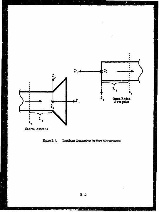
Ab
A
0~0
A A,
eSA Open.Ended
I a Waveguide
0
Source Antenna
Figure B-4. Cooidinaze Convetiado b Hemor Measurents
B-12
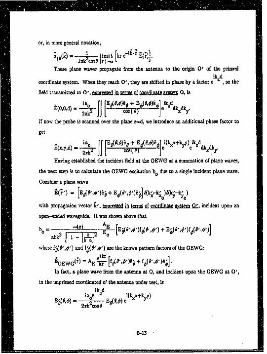
or, in more general notation,•lo~I •imi t [ e"'; *'9(",1
field transmitted to 01, exprsse in tR 2 coor a 0, is
-2A7 JJ1 r1If now the probe is scanned over the plane z=d, we introduce an additional phase factor to
get
2(x.yd =iao is, 0,0)6 + EO(8,O)6,6 e i(kxx+k).y) k zd
Having established the incident field at the OEWG as a summation of plane waves,
the next step is to calculate the OEWC excitation bo due to a single incident plane wave.
Consider a plane waveE ')= [Ete",•')a•+ E•(G',& )e]5(k-- )5kv--kv )
with propagation vector k', m in er R= 2 syste m .Q.ý, incident upon an
open--ended waveguide. It was shown above that
• ..41ri AE [E'8,,.)f0O,)abkI IF - 1&-j- -•2 L
where f•(9',@') and f(8',1&) are the known pattern factors of the OEWG:EOEWG(r) =AE"
In fact, a plane wave from the antenna at 0, and Incident upon the OEWG at 0',
in the unprimed coordinated o! the antenna under test, is
iaoe e(kxx+k.Y)E•(0,*) ='2xk2cos ,
B-13
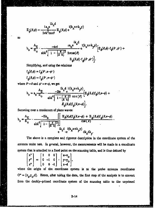
I lka~ d i,+k 9 )EPA,• = V0•(,4) ei~•ky
=2xk cosi ~9#so
ikzd
-=AE 4ri taoe ei(kxX+kyy)[E.(0 .).fO(O,,) +b° oo abkF7-W l_•_22%m(O)
Simplifying, and using the relations
fj$,(,) = f6(o • € )YOM,¢ = Y€,e,,•,,
where 1 =0 and 1 =s-0, we get
AE -2ieik z d i (kxx+ky) ,)ao-E&.- -7ze Coe a LEBiomfie'r-) +0 abk~j i-W.2 os
Summing over a continuum of plane waves:
AE -2ia [+ E,09 (09,(#)fOb° = '-oco*abD 1"ACost)
e3 T.e i xikx dkxdky.
The above is a complete and rigorous description In the coordinate system of the
antenna under test. In general, however, the measurements will be made in a coordinate
system that is attached to a fixed point on the scanning table, and is thus defined byI -1 0 Y-Yol,Z11 J 0 0 -1] [z-.dJrL' I= ' o 1 L- i J-O
where the origin of the coordinate system is at the probe antenna zoordinates
0" = (xoYod). Hence, after taking the data, the first step of the analysis is to convert
from the doubly-primed coordinate system of the scanning table to the unprimed
B-14
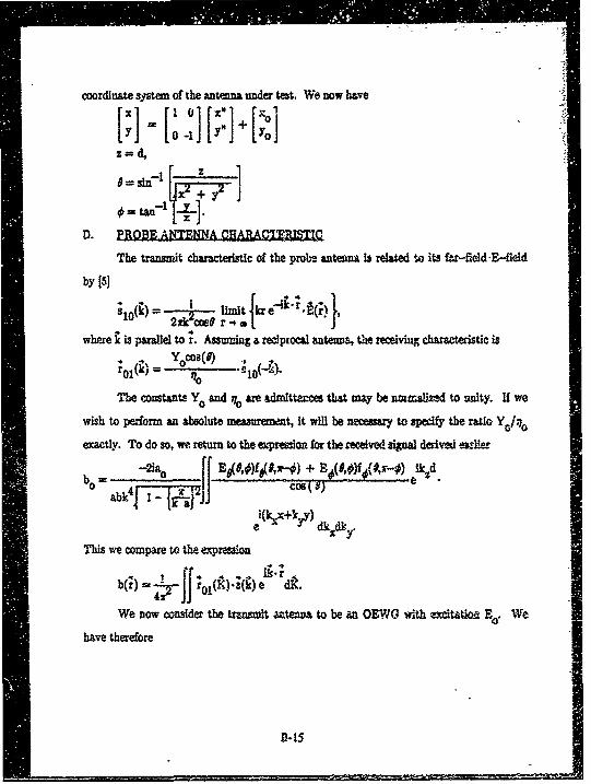
coordinate system of the antenna under tebt. We now have
z d,][01 ["o.:][ ]+[y :
D. PROBE ANTNNA MHARAIFQISTIC
The transmit characteristic of the prob- antennau Is related to its far-fielddE-,-1d
by [5]
811 limi t ° • '4'rj
" " 2xkcoe$ r -0 aL
where • is parallel to *. Assuming a redprocal anten-, the receiving characteristic is
Y cos(f)r01(k) = - -- 0(-L,)-
The constant Yo and io are admIttgrces that may be notlied to umity. If we
wish to perform an absolute me.•aurm t, It will be necessary to specify the ratio Yo
exactly. To do so, we return to the expression for the received signa derived eulier
-2i&o___ Ej(#,)f 6(,w-O) + lk(D,*)f@(Sa-.) 1k dbo= 0 I •o()-- -• "ablI r1- Cos ( )
i(k•+ky)
e dkdxky
This we compare to the expresion
4"T r01l.(k) e dK
We now conider the tran- t aztenv to be an OEWO with =xcitot;, Eo. We
have therefore
B-15
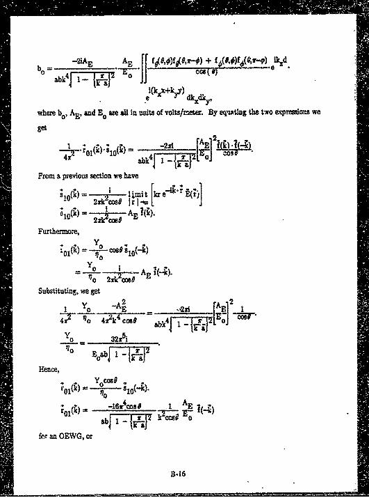
________ A I fj(9,q)f 9(D,x-j) + !f~(.O)f4(,.") lkzd.bo = - o (V
0 ab4{T{J~ 0dk~dky,
where bo, AF, and B0 are all in units of volts/meter. BY equting the two expressions we
get
1 *rn~)'1A~) -221 E ____
From a previous section we have
;1(i lj -I mi t 1r~ e ~r]
Furthermore,
I 1 (k) coeDsa 0(-k)10
Substituting, we get
YO -A' 21 ~ ~ o -2xi lA
-1- 4 l-D1-.4e 4 Cos# abo T 01
y 0 32A
Pence,Y Cos#
-l~) 6r4cosD . AE
er an OEG, or
3.16

-l8(ý) limit [kre r ()abYT1'-W Ocoeg Bo Ir ®r
where E(0,0) is the transmitted field due to an excitation E. in an OEWG
E. ~REa D =OF pyRAmIDAL HORN ANTENNA
The pyramidal horn probe antenna has the advantage that it has higher gain, which
increases the signal-to-noise ratio (SNR) on-axis. Of course, the horn's higher directivity
reduces the SNE. off-axis, and the presence of nulls in the horn pattern Is undesirable.
Since the horn antennak is well-characterized, it is also a good choice for a test antenna for
near-field antenna measurements.
The following discussion of the pattern of the pyramidal horn is taken from Balanis
[6]. The pyramidal horn geometry is shown in FiV, re B-5 (Balantis' Figure 12.18). The
following parameters are assumed to be known:
an wavegulde feed dimension (larger), along ix,
b wavegulde feed dimension (smaller), allong ~al horn dimension (larger), along ix,
ba horn dimension (smaller), alongY
p1 distance from aperture to B-plJane phase center,
P2adistance from aperture to fl-plane phase center,
Eo - wavegulde excitation (TB10 mode), and
A freem-space wavelength.
T~he tangential components of the E,- and H--felds at the horn aperture are
approximately
B~~(x~,y') +,2cs~x- B~(x'.y'
+ X21+7 I
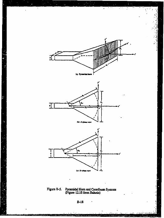
T iPimk hr
Fig= B-5
13-18
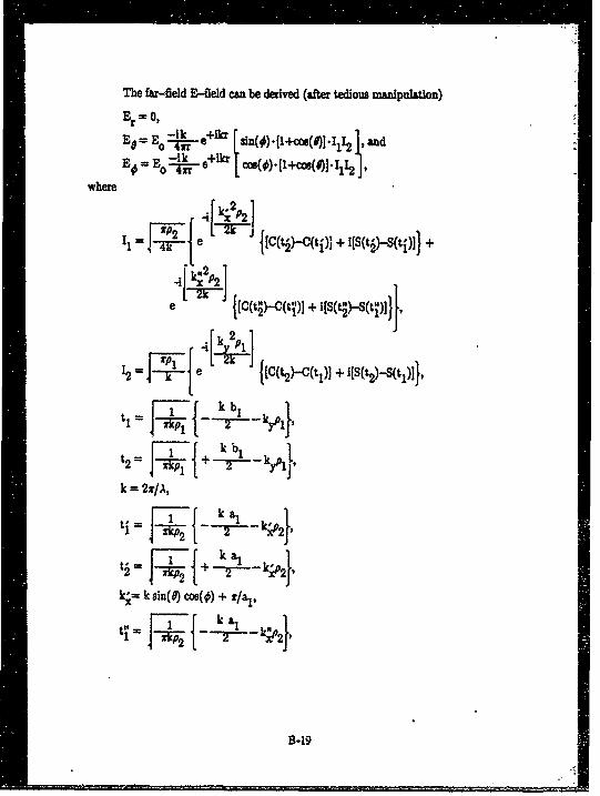
The far-field E--field can be derived (after tedious meanipulation)
Er =0,1k e+ikr an
E sE -1k 6eik co os()1+cws(I)J.I 1I2where
.4 [ kip2 P1
11 e fiC(t)-.c(ti) + [ti-til+
~ fi~i~e[ f I {C(t2.)C(tit 1)J + i[S(t2.Y-S I 1 1
k b,
k =2r/A,
k k sin($) cos(O) + /,
B-19

k = sin(O~coe(O) - j/l
k k =sn(f)sn(O);
and
C(x) = dt
,xd
5(x) = JPnHal. dt
are the Fresnel cosine and soe integrals.
We use the Narda 640 horn antenna at 10 Ghz driven by X-band waveguide.
Typical parameters are
a = .02286 mb = .01016 ma,= .0737 m,bl= .0544 ro,
Pl = .0916 m,
P2 = .1189 m.A = .03 m.
B-20

APPENDIX C
SCATTERING BY CONDUCTING SPHERE
The conducting sphere is a canonical object for which an analytical solution exists.
In this appendix we present a solution [191 for scattering by a perfectly conducting sphere,
followed by a derivation of the coordinate transformations necessary to utilize this solution
in verifying the measured scattering matrix.
For convenience, we will work initially in an unprhmed coordinate system. A
perfectly conducting sphere of radius a is placed at the origin (Figure C-i) and is
illuminated by a monochromatic incident plane wave traveling in the +6z direction with
x-polarizationi = kz ez
Einc =f Eo k" ) ex"
Dropping the e-40A denendency, write Lc in spherical form
o= F ) r..n+. _,.~(1) 1o[ oln "e2=n
where
fl=)(k2R)-Pl(cs# Cos ~ ap I(Coss)S sn " e0 -- Jn(k 2R) 80 sino
n)--n(n+l)- P(os)cos r +
IFit* 0(k21L) a$
1 6[k 2RJn(k2R)] n,8(k 2mo ONR) (o5sn
and
k, = propagation constant inside sphere,
k2 = propagation constant outside sphere and
C-1
AE
E
Fig=r C-1. Coaorciina Syute for Sphmr&=20dagngurdid
C-2
Rt = radius to observation point.
For R > a, the scattered field will have th4 form
n=1 (n7 [a
wh~er
4()-41)(k2FL).P1(Cose) coso e q'(1R) 81co
o~~~hn)( R)h kR. sn=el n(n+l)± n .~cocs 2r
I, #lk2 R4'h(I)(k2 R)J apn'(cwa)S 8(kf) A8N
1ý' O (k2R)J
We define
p=k 2.a,
so
k, -a= N-p.
The boundary condition at Rf= a requires that
ar = V,-, N P)~rJn(P)1 -P2 4 ,[Nj.(p
and
hr pln(Np)ýýTINpin(Np)M 2 pNJ(Np}j[pt.(p)1
The above equa~1ons are valid for a sphere with arbitrary dielectric properties. If
the sphere Is aluminum, and the surrounding medium is air, then
C-3
P, P2 = Po = 1.257 X 1o0- henry/meter,
el c2 = c = 8.&54 X 1- 12 farad/meter,
o1= 3.5 X 10 mho/meter, and
02 fo.
The general form of the propagation constant is
k2 = cp,2 + iw
= epw2(l + init
where
At f = 10 Ghz,
or 1- 6.3 X 10'' f 1w "
so
k2 ilt'1 p1} 1 , and
k * F" .6 x io6 / .•
Alsm.
kc2 g! 209.4 /mneter.
Choosing a 6-inch diameter sphere, a = .0762 meter, so
p=k 2
= 15.96
and
Np =, . 1.28 X 10⁵ /meter.
Since Np>> 1, we can use the asymptotic relations
ja(Np) g 1p
and
C-4

fv - sin [p - n
8(Np) ~-i N~~r
to sipiythe aoeequations for ar and brn' Yielding
ha1 (p v jn(P)+
Aftr heusal or o mnipultiniKR2+ 1 ceI IPcs)
1K2R w I )(SO)Er ~ ~ en~ f in( aplco)
and1
Er~ ~ ~~~. -K' JM 2~ P(OOI
APPENDIX D
SCATTERING BY CONDUCTING DISK
To calculate scattering from a conducting disk we use a physical optics solution due
to Capt. Keith Trott of RADC. Using the theory of physical optics 120], on a scattering
objectP% 2 fi H
whereJs total surface current,
a a unit normal vector pointing away from surface,
H aincident H field.
This is a good approximation for large objects but tends to break down with smaller
objects because it is not valid near edges. If the incident plane wave 9 is known, then one
can compute, in sequence, H, 3, and the vector potential
eJ ~dS,JTF,-• Iand the scattered E-field is
In the unprimed frame the disk is at the origin (Figure C-i), lies in the x-y plane,
and has radius a. It is illuminated from above the x-y plane by the incident wave vector~= -(co•ssin 1 .ex +smn smn.e +csOi.ez ) I6.
Assume i ties in the x--z planp, so 0•-0, and(a " - a + o. iy + cs
The observation location is also above the x-y plane at
r = x-6. + y'y + z'6z
= r (cosdn$ 6x + sl O sin6y + coe z),
so
D-l
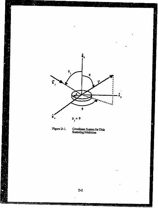
01 9=0
Figure D-1. COMHDini System forDisk0kuerng Fre~dici
D-2

- r -kir(sinfloosoinO + cosOicoeg.
The plane of incidence Is defined by ki and ez" There are two polazations of the incident
field - parallel and perpendicular to the plane of incidence. An arbitrary planar
illumination to with ki (0=O) can be expressed in terms of thome two polarizations:
A11 = Eol1 e (-cosiex + sinOz)
e y~
Considering the parallel polarization first, we have
27y-On the disk (0'=r/2) we use primed coordinates to indicate a source, so
Bol e 4 sin81cos0IV 6y
Then
= 2 8z 1= 4 fi•/2
-231 e kr'sine1coso'27 ix
The observation point is
; = I'r(cosqdnr + s.inof y + ccez)
while on the disk itself 8'=r/2, so
r IIj(cos0'6 + sino'a y)The factor I ;-;" I in the integral for A is
-- (rcos~n#n_',cos0') 2 +(rd '•si n#_r'sin 2)2 + r2cos20
= r + r,2 2rr_8InkW(#_0.)
In the denominator of the integral, I-'I cnM be approximated by !r1. in the
numerator phase factor, a better approximation is required. Ignoring quadratic terms
inside the radical, expanding in a Taylor series, and retaining the first two terms
g!-"~ r - r'sin6cosk--') 3
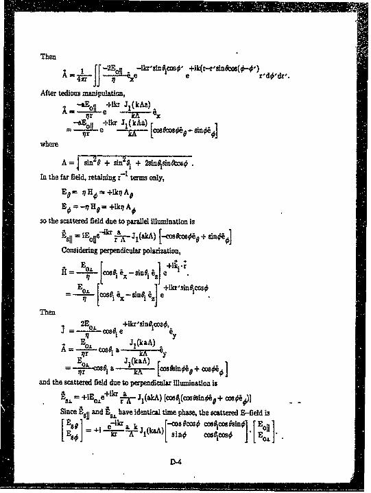
Then
A x- j 1-j-- 2- e e l~dl
After tedious manipulation,
a= j+lkI Jl(kA&)
e!ý fx'(,A [csecmOs6- snO,]where
In the far field, retaining r' tersu only,
EO =--qHe =+ikq AOso the scattered field due to parallel illumnination is
E51 ZE~e~=rAJ 1 (akA) [cOW&MOeO+ sino4
Considering perpendicular polarization,
EO [ 3 +ik.4 '/[cosei 1 sinei i5Je
Then2EI +lkr'sln9.coso,3= 0 cosO. e
A = -L c s e a (kaA ) .
_ ,r J (kaA),nr 0 A a L osdo + so
and the scattered field due to perpendicular Illumination is
Au +iE~e~ikr a y-j (akA) [co9j(csn$O+ cos$)]--Since~ and b. have identical time phase, the scattered B--field is
IE$# e7r k Ji(ka)j 3ecsi cos9~cosfsl EI oi
D-4

MISSION
OfRome.Air Development Center
JRADC plans and executes research, development, test andselected a quisiton Programs in -support of Command, Control,Communmication~s and Intelligence (C2I) activiies. Technical andengineering support within areas of competence is provided toES)) Program Offices (POs) and other ES)) elements lo
~3 perform efficlive acquisiion of V1 sytems. The areas ofS technical c~ompetence include communications, command andS control, battle management information processing, surveilance
sensors, intelligence data collection and handling, solid statesci'. nces, elect romagn etics, and propagation, and electronicreliability/m-aintainability and compatibilty.