Embed Size (px)
Citation preview

FINGERPRINT RECOGNITION USING PRINCIPALCOMPONENT ANALYSIS
A THESIS SUBMITTED TO THE GRADUATIONSCHOOL OF APPLIED SCIENCES
OFNEAR EAST UNIVERSITY
by
WAMEEDH RAAD FATHEL
IN PARTIAL FULFILLMENT OF THE REQUIERMENTSFOR THE DEGREE OF MASTER OF SCIENCE
In
COMPUTER ENGINEERING
NICOSIA 2014

DECLERATION
I hereby declare that all information in this document has been obtained and presented
in accordance with academic rules and ethical conduct. I also declare that, as required by
these rules and conduct, I have fully cited and referenced all material and results that are not
original to this work.
Name, last name: WameedhRaadFathel
Signature:
Date:

i
ABSTRACT
In this thesis fingerprint identification system was designed. A Principal Component
Analysis (PCA) is used to obtain the feature of images. Principal components analysis is one
of a family of techniques for taking high-dimensional data, and using the dependencies
between the variables to represent the image in a more tractable, lower-dimensional form,
without losing too much information. PCA is one of the simplest and most robust ways of
doing such dimensionality reduction. The simulation of the fingerprint identification system
using PCA has been performed. For comparative analysis a Fast Pixel Based Matching
(FPBM) method is also used for fingerprint recognition. FPBM is a method to extract the
features of images on the basis of fingerprint matching image areas and sub-pixel
displacement estimate using similarity measures. The application of PCA and FPBM to
recognition of fingerprint images is performed.
Classifications of image parameters are done by measuring Euclidian distance. The
given approach is used to classify the fingerprints to different patterns.The system can
identify persons according to these fingerprint patterns. The comparative simulation results of
described methods have been given. The developed system has a Graphical User Interface
(GUI) that contains many buttons and controls that allow the user to choose the necessary
method and drive the results. The system has been designed using MATLABpackage. Using
call-backs, you can make the components do what you want when the user clicks or
manipulated with keystrokes.
Key Words: Fingerprint Recognition Program, PCA, FPBM, Euclidean distance.

ii
ÖZET
Bu tezde, parmakizi tanıma sistemi dizayn edilmiştir. Görüntü özelliklerinin elde
edilmesinde Temel Bileşenler Analizi (TBA) kullanılmıştır. Temel Bileşenler Analizi (TBA),
yüksek boyutlu veri elde etmek için ve, çok fazla bilgi kaybetmeden değişkenler arasındaki
bağımlılıkları kullanarak görüntüyü daha uysal ve daha düşük boyutlu formda göstermek için
kullanılan teknikler familyasından bir yöntemdir. TBA, bu şekilde yapılan boyutsal
indirgemenin en basit ve en sağlıklı yöntemlerinden biri olmaktadır. TBA ileparmakizi tanıma
sistemisimülasyonuyapılmıştır. Parmakizi tanımada, karşılaştırmalı analiz için, Hızlı Piksel
Tabanlı Eşleşme (HPTE) yöntemi de kullanılmıştır. HPTE yöntemi, eşleşen parmakizi
görüntü alanlarına ve alt-piksel yer değiştirme tahminine dayanan görüntü özelliklerini,
benzerlik ölçüleri kullanarak ortaya çıkaran bir yöntem olmaktadır. Parmak izi görüntülerinin
tanınmasında, TBA ve HPTE uygulaması yapılmıştır.
Görüntü parametreleri sınıflandırılması, Öklid mesafesi ölçülerek yapılmıştır.
Parmakizlerini farklı desenlere sınıflandırmak için verilen yaklaşım kullanılmıştır. Sistem,
kişileri, bu parmakizi desenlerine göre belirleyebilir. Anlatılan işbu yöntemlerin
karşılaştırmalı simülasyon sonuçları verilmiştir. Geliştirilen sistemin, kullanıcının gerekli
yöntemi seçmesine ve sonuç çıkarmasına olanak tanıyan, birçok butonu ve denetimi içeren bir
Grafik Kullanıcı Arayüzü (GKA) mecuttur. Konu sistem, MATLAB paket programı
kullanarak dizayn edilmiştir. Geri-dönmeler kullanılarak, bileşenleri, kullanıcı tıklama veya
tuş-vuruşları ile manipüle edildiği zaman, sizin istediğinizi yapmaya yönlendirebilirsiniz.
Anahtar Kelimeler: Parmakizi Tanıma Programı, TBA, HPTE, Öklid Yer Değiştirme.

iii
ACKNOWLEDGMENTS
It is not possible to thank everybody who has had an involvement with me during the
course MSc. However, there are some people who must be thanked.
Firstly, I would like to thank my family and my parents whose encouragement, support
and prays has helped me achieve beyond my greatest expectations. I think them for their
understanding, love and patience. Without their help and support throughout the years it was
not possible for me to come this far.
I would like to thank my supervisor Prof.Dr.RahibH.Abiyev for his guidance and
encouragement throughout thesis.
I would like to thank my friends in Near East University MasterProgram (Ali Almansor,
Safwan Mohammad, ZaidDaood, AwadJehad, SipanSlivany, Ahmed Ashit, RashidZareen,
Muhammad Waheed,SaharShokuhi and FahimeMostoufi).
Finally, I would like thank my friends and all the people who helped me during my
master studying, especially Rami R. Mustafa friend of the study.

iv
DEDICATION
My parents: Thank you for your unconditional support with my studies I am honoured to
have you as my parents. Thank you for given me a chance to prove and improve myself
through all my walks of life. Please do not ever change. I love you.
My family,my daughters and my dear wife, thank you for believing in me: for allowing meto further my studies. Please do not ever doubt my dedication and love for you.
My brothers and sisters: hoping that with this research I have proven to you that these is no
mountain higher as long as God is on our side. Hoping that, you will walk again and be
able to fulfil your dreams.

v
CONTENTS
ABSTRACT ………………………………………………………………………... i
ÖZET ……………………………………………………………………………….. ii
ACKNOWLEDGMENTS ………………………………………………………….. iii
CONTENTS ………………………………………………………………………... v
LIST OF TABLES …………………………………………………………………. vii
LIST OF FIGURES ………………………………………………………………… viii
ACRONYMS AND UNITS ………………………………………………………... xi
INTRODUCTION …………………………………………………………………. 1
1. BIOMETRIC Systems ………………………………………………………....... 3
1.1 Overview ……………………………………………………………………….. 3
1.2 Biometric Systems ……………………………………………………………… 3
1.3 Biometric Classifications ………………………………………………………. 5
1.4 Summary ……………………………………………………………………….. 10
2. Fingerprint Identification ………………………………………………………… 11
2.1 Overview ……………………………………………………………………….. 11
2.2 Pattern Recognition …………………………………………………………….. 11
2.3 Fingerprint Recognition ………………………………………………………... 12
2.4 Fingerprint Classification ………………………………………………………. 12
2.5 General Form of the Fingerprint ……………………………………………….. 13
2.6 How the Fingerprint Recognition System Works ……………………………… 14
2.7 Fingerprint Representation and Feature Extraction ……………………………. 16
2.8 Fundamental Factors in the Comparison of Fingerprints ………………………. 20
2.9 Fingerprint Synthetic …………………………………………………………… 21
2.10 Methods of Extraction Properties …………………………………………….. 23
2.10.1 Histogram Projection Method (Histogram Projection) …………………….. 23
2.10.2 Method of Intermittent Properties (Discrete Feature) ………………………. 23
2.11 The Advantages of Using Fingerprint Recognition …………………………… 23
2.12 Disadvantages of Using Fingerprint Recognition System Finger …………….. 24
2.13 Summary ……………………………………………………………………… 25

vi
3. FEATURE EXTRACTION ……………………………………………………... 26
3.1. Overview ………………………………………………………………………. 26
3.2 Recognition System and the Problems of Large Dimensions …………………. 26
3.3 The Basic Steps of PCA Algorithm ……………………………………………. 28
3.4 Self-Fingerprint Eigenfinger PCA Algorithm Applied to the Fingerprint Images 30
3.5 Euclidean Distance ……………………………………………………………... 33
3.5.1 The Euclidean Distance Algorithm ………………………………………….. 33
3.5.2 Distance one-Dimensional …………………………………………………… 34
3.5.3 Distance bi-Dimensional …………………………………………………….. 35
3.5.4 Approximation for 2D Applications ………………………………………….. 35
3.5.5 Distance tri-Dimensional ……………………………………………………. 35
3.6 Fast Pixel Based Matching Using Edge Detection (FPBM) …………………… 36
3.6.1 Properties and the Contours ………………………………………………….. 37
3.6.2 Simplified Mathematical Model ……………………………………………… 37
3.6.3 Calculation of the First Derivative …………………………………………… 38
3.6.4 Calculation of the Second Derivative ………………………………………… 38
3.6.5 Operators for Edge Detection ………………………………………………… 38
3.9 Summary ……………………………………………………………………….. 40
4. DESIGN OF FINGERPRINT RECOGNITION SYSTEM.…………………….. 41
4.1. Overview ………………………………………………………………………. 41
4.2 General Structure of Fingerprint Recognition …………………………………. 41
4.3 Flowcharts of Feature Extraction Methods …………………………………….. 42
4.4 PCA Implementation .…………………………………………………………... 47
4.5 Implementation for Fast Pixel Based Matching (FPBM) ….…………………… 50
4.6 The Design of Fingerprint Recognition Program ………………………………. 51
4.7 Tested Samples …………………………………………………………………. 55
4.8 Results ………………………………………………………………………….. 64
5. CONCLUSION …………………………………………………………………. 66
REFERENCES …………………………………………………………………….. 68
APPENDIX A ……………………………………………………………………… 73
APPENDIX B ……………………………………………………………………… 77

vii
LIST OF TABLES
Table 1.1: Comparison of biometric technologies. The data are based on the perception
of the authors. High, Medium, and Low are denoted by H, M, and L,
respectively ……………………………………………………………….. 9
Table 4.1: Information about images and matrices in database in first test ……………. 56
Table 4.2: Information about tested image in first test …………………………………. 56
Table 4.3: Results for “2.tif” fingerprint image using PCA and FPBM ………………... 57
Table 4.4: Information about images and matrices in database in second test …………. 59
Table 4.5: Information about tested image in second test ……………………………… 59
Table 4.6: Results for “3.tif” fingerprint image using PCA and FPBM ………………... 60
Table 4.7: Information about images and matrices in database in third test …………… 62
Table 4.8: Information about tested image in third test ………………………………… 62
Table 4.9: Results for “7.tif” fingerprint image using PCA and FPBM ………………... 63
Table 4.10: Recognition rates of the system for tested images from first set ……….…. 64
Table 4.11: Recognition rates of the system for tested images from second set …….…. 65

viii
LIST OF FIGURES
Figure 1.1: Biometric Feature ………………………………………………………... 4
Figure 1.2: Biometric Systems (a) verification, (b) identification …………………… 4
Figure 1.3:Examples of biometrics are shown: a) face, b) fingerprint, c) hand
geometry, d) iris, e) keystroke, f) signature, and g) voice ……………… 5
Figure 1.4:Hand geometry biometric devices ……………………………………….. 5
Figure 1.5:Iris manipulations ……………………………………………………….. 6
Figure 1.6:Face recognition …………………………………………………………. 7
Figure 1.7:Vocal apparatus ………………………………………………………….. 7
Figure 1.8: Fingerprint Minutiae …………………………………………………….. 8
Figure 1.9: Electronic Tablet ………………………………………………………… 8
Figure 1.10: DNA recognition ……………………………………………………….. 9
Figure 2.1:The scheme shows the process of pattern recognition and image Processor 12
Figure 2.2: Fingerprints and a fingerprint classification schema involving six
categories: arch, tented arch, right loop, left loop, whorl, and twin
loop. Critical points in a fingerprint, called core and delta, are marked as
squares and triangles ……………………………………………………….. 13
Figure 2.3:The general shape of a fingerprint …………………………………………. 14Figure 2.4: System components fingerprint recognition ……………………………….. 15Figure 2.5:How fingerprint scanners recode identites …………………………………. 16Figure 2.6: Fingerprint sensors can be embedded in a variety of devices for user
recognition purposes ……………………………………………………….. 18
Figure 2.7: Characteristic patterns of fingerprints observed at the global level:
a) Ring to the left, b) ring to the right c) loop e) arc, and f) arc-shaped tent.
The squares indicate the singular points of the looptype; the triangles
indicate the singular points of the delta type ……………………………….. 18
Figure 2.8: Minutiae (black’s filled circles) shown on a portion of the fingerprint
image, position of the pores for sweating (blacks unfilled circles) along a
single ridge line ……………………………………………………………. 19Figure 2.9:Show in the example difficult to compare fingerprints: Fingerprints
in a) and b) may appear different to the untrained eye but are impressions
of the same finger. The fingerprints in c) and d) may look similar to the
untrained eye but actually come from different fingers ………………… 20

ix
Figure 2.10: Synthetic fingerprint images generated …………………………………... 21Figure 2.11: Fingerprint with minutiae highlighted related to: (a, b) scanner solid state,
(c) optical scanner ………………………………………………………… 22
Figure 3.1: Geometric interpretation algorithm PCA …………………………………... 29Figure 3.2:Beam represents a facial image ……………………………………………. 30Figure 3.3: Simulation and representation of self-fingerprint approach eigenfinger
approach; each fingerprint can be represented in the form of a linear fitting
of self- fingerprints ………………………………………………………… 33Figure 3.4: Determining the true Euclidean distance …………………………………... 34Figure 3.5:Edge detection ……………………………………………………………… 36Figure 4.1: General Structure of the program ………………………………………….. 41
Figure 4.2: Flowchart of converting 2D images to 1D …………………………………. 42
Figure 4.3:Flowchart for computing eigenvector ……………………………………… 43
Figure 4.4:Flowchart for extracting of PCA feature for tested image …………………. 44
Figure 4.5:Flowchart of recognition process from Euclidean distance ………………... 45
Figure 4.6:Flowchart of FPBM ………………………………………………………... 46
Figure 4.7:Original database images …………………………………………………... 47
Figure 4.8:Tested images set (1) ………………………………………………………. 47
Figure 4.9:Tested images set (2) ………………………………………………………. 48
Figure 4.10:Convert from RGB to grayscale ………………………………………….. 48
Figure 4.11:Effect of edge (image, ‘prewitt’) …………………………………………. 50
Figure 4.12: Start Program with default number of persons and images per Person ….. 51
Figure 4.13: Input test image by selection from that button …………………………… 52
Figure 4.14:Selection of database folder from that button ……………………………. 52
Figure 4.15: Creation database, number of person (2-20), number of images per
person (2-8) ………………………………………………………………. 53
Figure 4.16: Selection of recognition methods (PCA, FPBM) ………………………… 53
Figure 4.17: Results with successful recognition ………………………………………. 53
Figure 4.18a: Results with fail recognition …………………………………………….. 54
Figure 4.18b:Image when recognition is failed ………………………………………... 54
Figure 4.19: Helpful buttons: CLEAR, HELP, ABOUT and EXIT ……………………. 54
Figure 4.20:Snapshot for first sample …………………………………………………. 55

x
Figure 4.21:Tested image “2.tif” ………………………………………………………. 57
Figure 4.22: PCA results for tested image ……………………………………………… 57
Figure 4.23: FPBM results for tested image ……………………………………………. 57
Figure 4.24:Snapshot for second sample ………………………………………………. 58
Figure 4.25:Tested image “3.tif” ………………………………………………………. 60
Figure 4.26: PCA results for tested image ……………………………………………… 60
Figure 4.27: FPBM results for tested image ……………………………………………. 60
Figure 4.28:Snapshot for third sample ………………………………………………… 61
Figure 4.29:Tested image “7.tif” ………………………………………………………. 63
Figure 4.30: PCA results for tested image ……………………………………………… 63
Figure 4.31: FPBM results for tested image ……………………………………………. 63

xi
ACRONYMS AND UNITS
PCA Principal Component Analysis
FPBM Fast Pixel Based Matching
1 D 1 Dimensional
2 D 2 Dimensional
T Vector of reshaped database images
Prewitt To return the edges at those points where the gradient of not edged image is
maximum
RGB Red, Green, Blue
Edge MATLAB function read
M The mean vector
A The deviation vector
C Covariance matrix
L The surrogate of the covariance matrix
BMP Bitmap image file
RR Recognition Rate
TIF Tagged Image Format
U.are.U 4000
digital Persona
Biometric Finger Scan Device
Dpi Dots per inch
ATM Automated teller machine
PIN personal identification number
DNA Deoxyribonucleic acid

1
INTRODUCTION
Since the last century several biometrictechniques were used for identification of humans.
These techniques are: Iris recognition, Face recognition, Fingerprint recognition, Voice
recognition, etc. Each of these techniques has number of real life applications. [1]
Fingerprint recognition or fingerprint authentication refers to the automated method of
verifying a match between two human fingerprints. Fingerprints are one of many forms
of biometrics used to identify individuals and verify their identity. [1]
The aim of this thesis is the design of fingerprint recognition system using principal
component analysis. Fingerprint recognition system is divided into two main stages.The first
one is used to extract the feature from the fingerprint image, and the second stage is used for
classification of patterns. Feature extractingis a very important step in fingerprint recognition
system. This thesis touches on two major classes of algorithms used for extraction of the
feature of fingerprint images. The recognition rate of the system depends on the
meaningfuldata that are extracted from the fingerprint image.So,important feature shouldbe
extracted from the images. If the feature belong to the different classes and the distance
between these classesare big then these feature are important for given image. The flexibility
of the class is also important.There is no 100% matching between the images of the same
fingerprint even if they were from the same person.
Nowadaysthere have been designed a number of methods for feature extraction. These
are Principal component analysis,linear discriminant analysis, Fisher method, Multifactor
dimensionality reduction, nonlinear dimensionality reduction, Kernel PCA, independent
component analysis etc... The PCA is one of efficient method used for image feature
extraction. In the thesis the application of PCA method is considered for extractionthe feature
of fingerprint images. The classificationof the images can be implemented using different
classification algorithms: Euclidean Squared Distance, Hidden Markov Model (HMM), vector
quantization, k-means algorithm, or Artificial Neural Network (ANN).[2]In this thesis,
Fingerprint Recognition system was developed, and two techniques were used for feature
extraction. These techniques are PCA and Fast Pixel Based Matching (FPBM). Each of these
techniques was implemented on MATLAB and they are combined by using Graphical User
Interface (GUI).

2
The algorithm that was used for classification of fingerprint imagesuses Euclidean
Distance. If there is matching between the trained database images and the tested image, the
recognized image will be shown in GUI.But if there is no matching between them, a message
will appear to inform the user that this images in not recognized.
In this thesis the design of fingerprint recognition system using PCA and FPBM feature
extraction methods has been considered. The thesis includes introduction, five chapters,
conclusion, references and appendices.
Chapter 1 is devoted to the descriptions of biometric systems using fingerprint, iris, face,
voice, DNA and hand recognition techniques used in real life.
Chapter 2 describes the basic stages of fingerprint identification. The minute
characteristics of the images, the basic important meaningful feature of the fingerprint images
have been described. The extraction properties, advantages and disadvantages fingerprints have
been presented.
Chapter 3 explains the feature extraction methods of PCA and FPBM. The basic steps of
PCA and the recognition process using Euclidean distance are described. FPBM using edge
detection, the basic operations are presented.
Chapter 4 presents the design stages of fingerprint recognition system. General structure
of the system, the flowcharts of feature extraction methods are described. The thesis based on
two feature extraction techniques: PCA andFPBM.The fingerprint recognition system is
designed in MATLAB 2012a package using Graphical User Interface (GUI).
Finally, Chapter 5 contains the important simulation results obtained from the thesis.
3
1. BIOMETRIC SYSTEMS1.1 Overview
In this chapter the review of human identification systems is presented. The various
biometric techniques are described. The physiological and behavioural characteristics of
human which can be used as a biometric identifier to identify the person are presented.
1.2 Biometric Systems
Biometrics system is a method of mechanism to verify personal (person alive) based
on the unique physiological characteristics of the human body that is stored in the system
shareware. The biometrics of the human body in more ways personal check easy to use and
the most reliable and secure, they are not subject to theft or change, as they are of a permanent
and fixed. The verification system consists of a set of basic components: a device (system) to
save the image scanning (digital / Videos) the person's vital, and the treatment system and
comparison, and the application interface to show the result of the operation to confirm or
deny personal. The most important physiological properties that characterize the human body
are fingerprint.Here identification using a number of physiological properties of human
fingers is used.[3]
Biometric system is a device that is committed to identify a particular person using
biological characteristics of the individual. This feature can be grouped into two main
categories:
1. Physiological traits: show all static data from a person who is, fingerprints, iris pattern,
and shape of the hand or the face image.
2. Behavioural traits: it refers to the actions taken by the person concerned, and then
talking about his writings, and audio track, and method of pounding the keyboard.
In general, the physiological properties do not vary with the passage of time or for the
most part are subject to small changes while affected by the behavioural characteristics of the
psychological state of the individual. For this reason, identity verification systems based on
behavioural characteristics need frequent updates. The main task of a biological system is to
identify the individual.

4
Figure 1.1: Biometric feature.
The recognition system can carry two different meanings:
1. Identity verification: is to declare whether a person is really the person who claims to
be Figure 1.2.a.
2. Recognition of identities: It consists in determining whether a person matches with an
existing instance in the archive. It is not necessary to declare the identity Figure 1.2.b.
Figure 1.2: Biometric Systems (a) verification, (b) identification. [4]
BiometricFeatures
Physiology
Hand
Face
Iris
DNA
Digital Fingerprints
Behavioral
Voice
Line
Style From Keys

5
Biometrics are different types to extrapolate information from the human body, but it
is also important to understand that rely on a specific feature we will certainly be to build a
good system.
1.3 Biometric Classifications
All comparisons between the various techniques biometric As in all technologies listed in
the Figure 1.3 can be evaluated as an element so if we want to build programming that
comply with all requirements of the work and foremost must be safe, we need to in-depth
analysis of the characteristics of the application to create the necessary technology for use for
this reason.[5]
Figure 1.3:Examples of biometrics are shown: a) face, b) fingerprint, c) hand geometry, d) iris, e) keystroke, f)
signature, and g) voice. [5]
Hand Geometry: Human hand is a tool used in everyday life. It is a good way to know the
individual possesses something properties of exclusivity because of the length, width,
thickness, and in particular curvatures.[6]
Figure 1.4:Hand geometry biometric devices. [6]

6
Iris: Iris is one of the most accurate biometric in humans. They also excelled in accuracy
compared to using fingerprint iris. Additionally, it is difficult to manipulation iris the eye,
whether this manipulation by glasses or contact lenses or surgery of the eye. And the rest of
the identification process through the iris imprint as possible and easy to process. And so
this method has been adopted in many systems that require the disclosure of the identity of
the person security at airports and banks in automated teller machines and the high
efficiency of the iris. [7]
Figure 1.5:Iris manipulations. [7]
Featuring imprint iris as fixed and does not change over the life and therefore do not
need systems scanning the iris to renew their data stored in their own databases, as well as
the process of scanning the iris accuracy, efficiency and high efficiency as they managed to
excel through several stages on the accuracy of fingerprint or retina eye or the palm of the
hand as it also feature easy to use.

7
Face: The first thing we do is to identify the person to look at them in the face, and we
certainly are not used to analyse fingerprints or the iris of the eye. Research shows that when
we look at people tend to focus on the parts as the dominant big ears, aquiline nose, etc... It
is also found that the internal characteristics (nose, mouth and iris) and (head shape, hair).[8]
Figure 1.6: Face recognition. [8]
Voice: Even a person's voice is considered an element of biometric recognition. Biometric
feature does not have sound levels of stability.[9]
Figure 1.7:Vocal apparatus. [9]

8
These devices are shown in Figure 1.7 is responsible for issuing the votes of the mouth,
which in fact can change from person to person and produces a sound wave sound when air
from the lungs through the trachea and vocal cords and is characterized by this source by
dealing with the excitement, pressure and vibration, murmur or a combination of these.
Fingerprints: Fingerprint is the best system to verify the identity and the most common
biological characteristics oldest and widely used in technological applications, which
depend on the lines and formations deployed on the surface of human skin at the
fingertips, where readers can these patterns, analyse and identify them and stored.[10]
Figure 1.8:Fingerprint Minutiae. [10]
Signature: There is always a difference in every sample of that person's signatures
resulting from the movement of the hand in the way of drawing the letters of the name or
in the way of drawing a certain curve or certain angle or certain lines in the signature
itself. Those differences may affect the results.[11]
Figure 1.9: Electronic tablet. [11]

9
DNA: Deoxyribonucleic Acid (DNA) is the one-dimensional ultimate unique code for
one’s individuality, except for the fact that identical twins have identical DNA patterns. It
is, however, currently used mostly in the context of forensic applications for person
recognition.[12]
Figure 1.10: DNA recognition. [12]
Table 1.1: Comparison of biometric technologies, the data is based on the perception of the
authors. High, Medium, and Low are denoted by H, M, and L, respectively. [13]
Factors
Uni
vers
ality
Dis
tinct
iven
ess
Perm
anen
ce
Col
lect
able
Perf
orm
ance
Acc
epta
bilit
y
Cir
cum
vent
ion
Biometric
identifier
Hand Geometry M M M H M M M
Iris H H H M H L L
Face H H M H L H H
Voice M L L M L H H
Fingerprint M H H M H M M
Signature L L L H L H H
DNA H H H L H L L

10
1.4 Summary
The feature of vital physiological characteristic of every human, such as fingerprint and
eye, face, hand, voice and signature have achieved significant improvement in personal
identification. The extracted featureof this biometrics have made a significant achievement in
reducing many of the problems and weaknesses that faced with the traditional way ofverifying
the identity (persons) using passwords. Despite the degree of high security achieved by
thesetechniques the accuracy recognition systems did not reach to 100% yet.For this reason
the design of new techniques for feature extraction and image recognition become important
computer science.

11
2. FINGERPRINT IDENTIFICATION
2.1. Overview
Due to the increased use of computer technologies in modern society, the growing
number of objects and the flow of information that must be protected from unauthorized
access, the information security problem become more and more urgent.In such circumstances
the use of biometrics technology for personal identity to protect access to sources of
information is required.
The use of biometrics to verify the identity involves the use of physical characteristics
such as face, voice or fingerprint, for the purpose of identification. Fingerprint matching is the
most successful biometric identification technology for its ease of use, and the absence of any
interference reliability. The basic characteristics of fingerprints, their representation, minute
characteristics and feature extractions stages are considered in this chapter.
2.2. Pattern Recognition
The pattern recognition is one of the branches of image processing and artificial
intelligence as it aims to find or develop techniques to identify a particular pattern or shape. It
has important and useful applications as characters distinction and gets to know people,
shapes and is also used in medical fields.
Pattern recognition is one of the important branches in the field of digital image
processing; this area took considerable attention by many researchers which have proposed
many methods and techniques in this area.[14]
Image analysis and extraction characteristics of the most important and follow the key
steps for the purpose of pattern recognition, despite the fact that there are many methods used
such as neural networks and other analysis and digital image processing traditional, but
evolution in the field of image processing led to the discovery of modern methods which can
be used in the process of identifyingpatterns.

12
Figure 2.1: The scheme shows the process of pattern recognition and image processing.
2.3. Fingerprint Recognition
It has become easy toidentify fingerprints mechanism expeditious manner, due to
advances in the capabilities of computers. And is what is known as technology, fingerprint
recognition; terms refers to the verification mechanism of match fingerprints man using
characteristics and unique feature of a fingerprint. Fingerprint identification is one of the most
popular biometrics, and the fingerprints of the oldest adjectives that have been used for more
than a century for identification.
The use of fingerprints due to the uniqueness of the fingerprints was excellence and
persistence. Valtferd intended to distinguish each person unique fingerprint shape, there is no
two people in the world have the same fingerprint. There is a possibility of 64 billion a chance
to fully match the fingerprint with another person. [15]
The fingerprints that cannot be matched even for twins, it is possible to be very similar
when viewed with the naked eye, but this does not mean conformity never. [16] And
consistency means the indivisibility of change, "it has been proved that human fingerprints
breed with their shape remains unchanged until his death. [17] Unless there is an emergency
such as sickness, injury or burn.
2.4. Fingerprint Classification
In order to reduce the time needed to search for fingerprint matching in the database of
fingerprints, especially in the case of size database, it is recommended to classify fingerprints
in an accurate and logical, and thus is matched template fingerprint input with a subset of the
templates stored in the database.
ImageClassification&
Identification of anImage
PatternRecognition
ImageProcessing

13
Figure 2.2: Fingerprints and a fingerprint classification schema involving six categories: arch, tented arch, right
loop, left loop, whorl, and twin loop. Critical points in a fingerprint, called core and delta, are marked as squares
and triangles [18]
2.5. General Form of the Fingerprint
Notes the general shape of the fingerprint is that its surface is coated with accurate parallel
lines rising from the surface of the skin (epidermis) and are called lines salient or rims
(Ridges) and between those lines there are lines of low accuracy and these lines are called low
lines or cracks (Furrows) or valleys (Valleys) which are not going in one straight course but
have a variety of forms many, the mismatch in forming multi circles about the midpoint,
while others are in the form of lines sloping to the right or the left, and so on up to the lines
curved starting point and end of the second and other formats.[19]
The use of Biometric vital standards is one of the most important Metrology used in the
disclosure of the identity of persons. The Babylonians used first hand fingerprint in the mud
to prove ownership (as a signature). Figure 2.3 illustrates the general shape of the fingerprint.
For the purpose of the using parts of the partial properties vital to the standards, it must
provide the following four conditions:

14
Figure 2.3:The general shape of a fingerprint. [20]
Universality.
Distinctiveness.
Permanence.
Collectability.
2.6 Components of FingerprintRecognition
The system is able to recognize someone on the basis of the mark needs to match these with
the specifications of the fingerprint real person called the process of introducing the user to
the fingerprint system for the first time to register, as shown in Figure 2.4 in this case, the
fingerprint attributes stored in the form of a "template" in the database.
The system of fingerprint identification captures the fingerprint image by the scanner.
And a fingerprint scanner is an electronic device used to capture an image directly to a
fingerprint. Then it processes the fingerprint image, and then extracts and measures the details
and unique feature using algorithms to create a template. These templates are stored in a
database within the system, and can also be stored on a smart card.

15
Figure 2.4: System components fingerprint recognition.
If you use the user in the system every time you need to define his character, put his
finger on the scanner, the system creates a template. After that the system will match this
template entrance in one of two ways, according to the quality of the system:[21]
Identification system to make sure: Authenticates the system to make sure the identity of
the person identity by comparing the input fingerprint template with your fingerprint
template stored in the system. And the process of comparison between the template and the
stored template entrance just to make sure that the identity of the person to be incorrect. And
recommended the adoption of the way "to make sure identity" when a large number of users.
System identification: The system detects a person's identity by searching the full templates
stored in the database to match with the template fingerprint entrance. The comparison
process is one template (template entrance) to a set of templates to determine the identity of
the person. Found closely with one of the samples it recognizes the person otherwise it
refuses to recognize it. Some may believe that the process of matching fingerprints are on
the entire fingerprint, and this is a misconception, as it is if it also will require a high-energy
, and be easy to steal the printed data . In addition to that dirt or distortion process leading to
mismatch two images of the same fingerprint. So it's an impractical way. Instead, the
majority of fingerprint recognition systems comparison between certain attributes and
feature of the fingerprint.[22]
MatchingResult
Input
Fingerprintclassification
Fingerprintenhancement
Orientationfield
estimation
Fingerprintsegmentation
Fingerprintridge thinning
Minutiaeextraction
Minutiaematching
Minutiaetemplate

16
Systems use fingerprint recognition algorithms are too complex to analyse and
recognize these details.The basic idea of measuring sites this detail, an end similar to the
method of identifying the somewhere.Where you recognize the shape is formed by different
details when drawing straight lines.
Figure 2.5: How fingerprint scanners recode identities. [22]
If there was combined for the two same extrusion endings and the same dendrites;
they form the same shape and the same dimensions. There is a high probability to be the same
person. The system does not need to be registered every detail in both samples. But enough
for a certain number of details even compares them.This number varies depending on the
system fingerprint recognition. [23]
2.7 Fingerprint Representation and Feature Extraction
The representation issue constitutes the essence of fingerprint recognition system
design and has far-reaching implications for the design of the rest of the system. The pixel
intensity values in the fingerprint image are typically not invariant over the time of capture
and there is a need to determine salient feature of the input fingerprint image that can
discriminate between identities as well as remain invariant for a given individual. Thus the
problem of representation is to determine a measurement (feature) space in which the
fingerprint images belonging to the same finger form a compact cluster and those belonging
to different fingers occupy different portions of the space. [24]

17
The main feature of a fingerprint scanner depends on the specific sensor was used,
which in turn determines the feature that the resulting image, such as:
Dpi (dot per inch or dots per inch) is a measure of the scanning resolution expressed as the
density of points per unit of measurement.
Useful area of acquisition, or the dimensions of the sensitive surface, p influence the number
of distinctive feature acquired, but also the accuracy: sensors with smaller areas have lower
costs but also lower accuracy in terms of recognition which may be partially lower precision
in terms of recognition that can be partially offset with appropriate algorithms for the re-
tread from a set of smaller images and partially overlapping.
Dynamic range or the number of graylevels quantized by the scanner, which translates into a
greater or lesser precision in the representation of the details.
A sample of fingerprints show different types of characteristics in function of the level
of magnification at which is analysed more precisely according to the level of magnification
at which it is analysed, more precisely can be reduced to three relevant levels of observation
that exhibit distinctive structures votes for recognition: the global level, the local level and
that ultra-fine.
At the global level, the flow of ridge lines outlining various possible configurations.
The so-called singular points, which may be of the delta or ring, serve as control points
around which the lines can wrap. The singular points and the gross form of the lines have
considerable importance for the classification and indexing of fingerprints but are not
sufficiently distinctive for fingerprint recognition, but are not sufficiently distinctive for
accurate recognition. Additional feature detectable at this level are the shape of the
fingerprint, orientation and frequency of' image. [25]

18
Figure 2.6: Fingerprint sensors can be embedded in a variety of devices for user recognition purposes. [25]
Figure 2.7: Characteristic patterns of fingerprints observed at the global level:
a) Ring to the left, b) ring to the right c) loop e) arc, and f) arc-shaped tent.
The squares indicate the singular points of the loop type; the triangles indicate the singular points of the
delta type. [25]
19
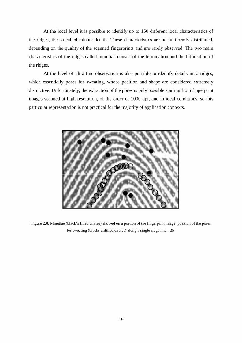
At the local level it is possible to identify up to 150 different local characteristics of
the ridges, the so-called minute details. These characteristics are not uniformly distributed,
depending on the quality of the scanned fingerprints and are rarely observed. The two main
characteristics of the ridges called minutiae consist of the termination and the bifurcation of
the ridges.
At the level of ultra-fine observation is also possible to identify details intra-ridges,
which essentially pores for sweating, whose position and shape are considered extremely
distinctive. Unfortunately, the extraction of the pores is only possible starting from fingerprint
images scanned at high resolution, of the order of 1000 dpi, and in ideal conditions, so this
particular representation is not practical for the majority of application contexts.
Figure 2.8: Minutiae (black’s filled circles) showed on a portion of the fingerprint image, position of the pores
for sweating (blacks unfilled circles) along a single ridge line. [25]

20
2.8 Fundamental Factors in the Comparison of Fingerprints
Experts in the analysis of fingerprints take into account a number of factors before
stating that two fingerprints belong to the same individual. These factors are:[26]
Concordance in the configuration of the global pattern, which implies a type common to the
two compared fingerprints, common to the two compared fingerprints.
Qualitative agreement, which implies that the corresponding minute details are identical.
Quantitative factor that specifies the minimum number of minute details that must match
between the two fingerprints (at least 12 according to the directives forensic U.S.).
Correspondence of the minute details that need to be identically interrelated.
Figure 2.9: Show in the example difficult to compare fingerprints: Fingerprints in a) and b) may appear different
to the untrained eye but are impressions of the same finger. The fingerprints in c) and d) may look similar to the
untrained eye but actually come from different fingers. [26]

21
2.9 Fingerprint Synthetic
The performance evaluation is strongly influenced by dataset on which it is conducted.
The conditions for acquiring the database size and the confidence interval should be specified
in the results.
Since the availability of large database on which to perform the testing is the main
bottleneck for effective validation of results, but their cost in terms of time can be
prohibitively expensive, have been proposed methods of generating synthetic (algorithmic)
Fingerprint generating synthetic (algorithmic) fingerprint.
The purpose is the creation of vast database of fingerprints valid for the testing of the
methods of recognition.
Fingerprints synthetic can effectively simulate the following characteristics of the
impression of a fingertip real:[27]
Different contact areas.
Non-linear distortions produced by a non-orthogonal pressure of the fingertip on the
sensor.
Variation in the thickness of the ridges (ridges) due to intensity of the pressure or the
conditions of the epidermis.
Minor cuts and / or abrasions and other type of noise.
Figure 2.10: Synthetic fingerprint images generated. [27]
The premise of the method is that the advent of fingerprint sensors in solid state
which, moreover, is favouring a wider uptake of this biometric, enables a contact area with
the fingertip very limited and consequently acquisition of a reduced amount of information
discriminating (typically for a sensitive surface of 1.5×1.5 cm are obtained 300×300 pixels at
500 dpi).
22
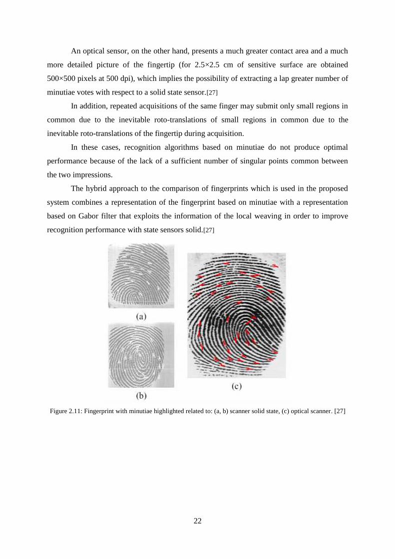
An optical sensor, on the other hand, presents a much greater contact area and a much
more detailed picture of the fingertip (for 2.5×2.5 cm of sensitive surface are obtained
500×500 pixels at 500 dpi), which implies the possibility of extracting a lap greater number of
minutiae votes with respect to a solid state sensor.[27]
In addition, repeated acquisitions of the same finger may submit only small regions in
common due to the inevitable roto-translations of small regions in common due to the
inevitable roto-translations of the fingertip during acquisition.
In these cases, recognition algorithms based on minutiae do not produce optimal
performance because of the lack of a sufficient number of singular points common between
the two impressions.
The hybrid approach to the comparison of fingerprints which is used in the proposed
system combines a representation of the fingerprint based on minutiae with a representation
based on Gabor filter that exploits the information of the local weaving in order to improve
recognition performance with state sensors solid.[27]
Figure 2.11: Fingerprint with minutiae highlighted related to: (a, b) scanner solid state, (c) optical scanner. [27]

23
2.10 Methods of Extraction Properties
There are many methods of universality in the application to distinguish the properties
of the image in the manner Off-line.
2.10.1 Histogram Projection Method (Histogram Projection)
This method was provided since 1956 by KloparmanGlauberman systems
distinguishing images used by electronic devices (Hardware OCR) this method is used Mostly
in the cutting process (Segmenting) of the image as well as to discover whether the image has
been rotated. This method is based on the account number of points in the image horizontally
and vertically. [28]
2.10.2 Method of Intermittent Properties (Discrete Feature)
Can draw some characteristics such links a number of type T, and a number of points
of contact of the type X, and the number of points and bending, and the proportion of width to
height in the rectangle that surrounds the image, and the number of points isolated, and a
number of endings in four horizontally directions and while the position of the center of
gravity depends on the installation axes. [28]
2.11 The Advantages of Using Fingerprint Recognition
The advantages of using a system fingerprint to identify the following:
1. The uniqueness of each finger everyone distinctive fingerprint. [24]
2. Cannot guess a fingerprint, such as what we can guess the password.
3. Provided it with you everywhere, unlike magnetic ID card.
4. Finger scans process easy and safe healthy. There is no health damage because they do
not depend on the laser beam or X- ray or something like that.
5. Research and development in this field is very fast and powerful. [24]
6. If we want to increase the level of security identification, we can record and recognize
more than one finger imprint per person (up to ten fingers) and fingerprint each finger
distinctive and unique.
7. Hardware fingerprint recognition with relatively low prices compared to other
identification systems.

24
2.12 Disadvantages of Using Fingerprint Recognition System Finger
Although the effectiveness of fingerprint recognition systems in finger protection
systems but it has disadvantages, including the following:[28]
1. That biometrics has always been susceptible to deception smart, where devices can
fool some of the fingerprint recognition by anthropomorphic design of a finger, And in
the worst cases, the offender may cut off the hands of someone so that he can pass
system.
2. May be the most serious disadvantages of biometrics, that if one was able to steal your
fingers fingerprint cannot be used as a check to life only after the confirmation of the
execution of all copies, because you will not get a new imprint like if stolen ATM card
or your PIN number.

25
2.13 Summary
In this chapter, we identify the structure of fingerprint identification system, its basic
components. Fingerprint characteristics, extract details of feature, fingerprints, and the
importance of a system of fingerprint identification are described. Feature extraction methods,
the advantages and disadvantages of fingerprint recognition are described.

26
3. FEATURE EXTRACTION
3.1 Overview
The Principal Component Analysis (PCA) is a method of family data analysis and
more generally multivariate statistics, which involves transforming interrelated variables
(called correlated in statistics) in new variables, uncorrelated each other. These new variables
are called "principal components" or main roads. It allows the practitioner to reduce the
number of variables and make less redundant information.
It is an approach that includes both geometric (the variables are represented in a new
space, according to maximum inertia directions) and Statistics (research on independent axes
to better explain variability - the variance - the data). When you want to compress a set of N
random variables, the first n lines of the principal component analysis is a better choice in
terms of inertia or variance.
Edge detection is the name for a set of mathematical methods which aim at identifying
points in a digital image at which the brightness changes sharply or, more formally, has
discontinuities. The points at which image brightness changes sharply are typically organized
into a set of curved line segments termed edges. The same problem of finding discontinuities
in 1D signal is known as step detection and the problem of finding signal discontinuities over
time is known as change detection. Edge detection is a fundamental tool in image
processing, machine vision andcomputer vision, particularly in the areas of feature
detection and feature extraction.
3.2 Recognition System and the Problems of Large Dimensions[29, 30 and 31]
Problems usually appear in fingerprint recognition systems when dealing with systems
large-dimensional images can make many improvements and cross-matching and data transfer
existing data to lower dimensions. Thus we may have dimensionality reduction of the original
image with large dimensions of the new image with smaller dimensions.
For example, we have the followingT
1 2 NX X , X ], X[ (3.1)
and that within the space of N after the author, by reducing the dimensions we move to the
last beam to any space consisting of Kso that after K< N.
T1 2 ky y , y ], y[ (3.2)

27
The decrease Dimensions in turn leads to the loss and the loss of information, but the
goal of the algorithm is to reduce the dimensions of the PCA data while retaining as much as
possible and important part of the information in the original data.
This process is equivalent to retain as much as possible of the variations and changes
contained within the original data.
The PCA calculates linear transformation T, which compares the data contained
within the space dimensions to the information to approve it within a partial-dimensional
space, at least, as the subject below:
1 11 1 12 2 1 N N
2 21 1 22 2 2 N N
k k 1 1 k 2 2 k N N
y t x t x ... t xy t x t x ... t x...y t x t x ... t x
(3.3)
Or in other words
Xy T (3.4)
whereas
11 12 1
21 22 2
1 2
N
N
k k kN
t t tt t t
T
t t t
(3.5)
The optimum conversion T is a conversion that where the value || X |y | minimal.
Depending on the theory of PCA, it can define a space with dimensions of at least optimized
through the use of the best X-self eigenvectors own matrix variation of the data covariance
matrix of the data. We mean: the rays of self-approval of the values of self-largest largest
eigenvalues of the matrix, contrast, and also referred to as the basic components "principal
components".

28
3.3 The Basic Steps of PCA Algorithm
Suppose that 1 2I , I , , IM a set of M beam, each beam has the following
dimensions 1N .
First step: we calculate the average beam for a given radiation
1
1ĪM
iiM
(3.6)
Second step: We are Normalize each scan, and put it through the center of the beam, which
was calculated in the first step
Īi i (3.7)
Third step: the formation of the matrix 1 2, , , MA Dimensions N M .
Fourth Step: we calculate the variance matrix (covariance matrix)
1
1CM
T Tn n
nA A
M
(3.8)
It is a matrix dimensions N N . [29]
Fifth step: Calculate the eigenvalues 1 2, ,, N and self-rays 1 2u ,u , ,uN matrix C
(Assuming that 1 2, ,, N ). [29]
Since the matrix C Symmetrical, the 1 2u ,u , ,uN form the a set of X-basis
vectors, and therefore any beam I within the same space can be written in the form of a linear
fitting of radiology self-linear combination of the eigenvectors, using the radiation that has
been holding normalize them, and therefore we have the following:
1 1 2 21
ĪN
N N i ii
y u y u y u y u
(3.9)
Sixth step (Dimensions loss): It is here in this step represent each beam Iby retaining only
approved for the largest values K intrinsic value:
1 1 2 21
ˆ Īk
k k i ii
y u y u y u y u
(3.10)
Where K < N, in this case, the Î convergence I so that it is || I | Î | smaller.

29
Therefore, the linear transfer T included within the PCA defined by the basic
components of variance matrix covariance matrix.
11 21 1
12 22 2
1 2
k
k
N N k N
u u uu u u
T
u u u
(3.11)
The PCA drop data along the trends that differ by more data than others Figure 3.1
These trends are identified through self-ray contrast matrix (eigenvectors of the covariance
matrix) of the values of self-approval largest (largest eigenvalues).
The magnitude of the size and amplitude values compatible with the self-variation data along
trends self-rays.
Figure 3.1: Geometric interpretation algorithm PCA. [32]
To decide what the number of principal components is core components that we need to keep
(mean value of K), it can be used the following criteria:
1
1
kii
Nii
t
(3.12)
Wheretis the threshold (for example: take the following values of 0.8 or 0.9) and tvalue that
specifies the amount of information that will be kept within the data. What determines the
value of t ; it can then determine the value of K.
We cannot say that the error due to dimensional reduction step given the following words:
1
12
N
ii k
e r r o r
(3.13)

30
It should be noted that the principal components based on units used to measure the
original variables as well as on the field values that are assumed. Therefore, it should always
unite us (to make it a standard) data before using the algorithm PCA.
3.4 Self-Fingerprint EigenfingerPCA Algorithm Applied to the Fingerprint Images
The approach to facial self (eigenfinger approach) algorithm uses PCA to represent the
fingerprints within the subspace low-dimensional, and is extracted this space by taking
advantage of the X-self (eigenvectors) best any fingerprints self (eigenfinger) matrix contrast
portraits (covariance matrix of the fingerprint images ).[33]
Assume that we have a group of M-fingerprint training 1 2I , I , , IM each
fingerprint image has the following dimensions N N . The basic steps necessary to
implement the PCA algorithm on a set of pictures fingerprints:
First step: are converted to represent each fingerprint image iI Dimensions of the following
N N to single beams i the following dimensions 2 1N . This process can be accomplished
simply by row lines and one of them after the other, to turn from the matrix to the single beam
(as in Figure 3.2).
Note: You must, of course, before this step that may have been done along the images and
measured relative to each other.
Figure 3.2: Beam represents a facial image. [34]

31
Second step: Central fingerprint is calculated through the following relationship:
1
1 M
iiM
(3.14)
Third step: Normalize is done for each beam images iT and put forward through the middle
of the fingerprints are as follows:
i i (3.15)
Fourth step: The formation of the matrix 1 2, , , MA consisting of 2N M .
Fifth step: is calculated contrast dimensional matrix containing variations fingerprints.
According to the method of PCA, we need to calculate the self-ray iu matrix TAA . But a very
large matrix ( . .i e equal to expel 2 2N N ), and therefore, it is not feasible that we calculate
her self-rays. Instead, we will take into account Self-rays iV matrix TA A .Which in turn is
much smaller than the matrix (i.e., that the dimensions M M ).And then we calculate self-
rays of the matrix TAA from self-rays of the matrix.
Sixth step: There we calculate the self-ray iV of the matrixAAT. We can simply show the
relationship between iu and iV . As the iV X is a self-matrix TA A , they bring the following
relationship: Ti i iA A V V That's where i represents the values of self-approval.
If we beat both parties within the following matrix equation A Then we will get
Ti i iAA AV A V (3.16)
Or
i i iC A V A V or i i iC u u (3.17)
Each of the AATand ATA has the same values as self-linked self-rays through the following
relationship:
i iu A V (3.18)
It is worth to note that the matrix TAA can have up to 2N self-beamed, while the matrixTA A Can have up to M self-ray.

32
Rays can show that the self-matrix TA A Better compatibility M ray self-matrix TAA (In
other words, self-rays agree eigenvalues larger).
Seventh step: Self-rays are calculated iu the matrix TAA Using the relationship
i iu A V (3.19)
Note: You must do to normalize iu So that it is || || 1iu .
Eighth step: (D-loss) are represented by each fingerprintT Transient retain only the values
that greater consensus K intrinsic value:
1 1 2 2 11
ˆk
k k ii
y u y u y u y u
(3.20)
Figure 3.3 below provides us emulates to self-fingerprint approach eigenfinger
approach. In the first row, is showing a group of self-fingerprints eigenfinger (no self-
compatibility fingerprints great eigenvalues) comes the phrase "self-fingerprint" by the fact
that self-rays look like ghost images).
The second row, it shows us a new fingerprint, was expressed in the written form of
the installation of self-fingerprints.
Using PCA, each fingerprint image T can be represented within the space with
dimensions smaller than the dimensions of the original image, using the linear expansion
coefficients:
1
2
k
yy
y
(3.21)

33
Figure 3.3: Simulation and representation of self-fingerprint approach eigenfinger approach; each fingerprint can
be represented in the form of a linear fitting of self- fingerprints. [35]
3.5 Euclidean Distance
In mathematics, the Euclidean distance is the distance between two points that is the
extent of the segment joining the two extreme points. By using this formula as distance,
Euclidean space becomes a metric space (in particular). The traditional literature refers to this
metric as Pythagorean metric.
3.5.1 The Euclidean Distance Algorithm
Tools Euclidean distance describes the relationship of each cell to the source or group
of sources on the basis of the distance along a straight line. There are three Euclidean tools:
[36]Euclidean distance of the instrument shows the distance from each cell of the raster to the
nearest source.
Tool Euclidean direction indicates the direction from each cell to the nearest source.
Symbol distribution Euclidean distance (Euclidean Allocation) is used to determine the cells
which should be assigned to the source based on the maximum proximity.
Euclidean distance is calculated from the sources to the center of a cell from the center
of each surrounding cell. In the tools to determine the distance the true Euclidean distance is
calculated to each cell. From a conceptual point of view, the Euclidean algorithm works as
follows. For each cell, the distance to the source of each cell is calculated by computing the

34
hypotenuse, and the values are the legs of _x max and _y max . This calculation gives a true
Euclidean distance, and not the distance between cells. Measure the shortest distance to the
source, and if it is less than a predetermined maximum distance, location on the output raster
is assigned a value. [37]
Figure 3.4: Determining the true Euclidean distance. [38]
The output values for the raster Euclidean distance - distance values denominated
floating-point numbers. If the cell is located at the same distance from two or more sources, it
will be attributed to the source, which was first found in the scanning process. The scanning
process cannot control you.
Description above - this is a conceptual description of how the values were obtained.
The actual algorithm computes the information using a twice- scanning. This process sets the
speed of the tool, which does not depend on the number of cell sources, the distribution of cell
sources and a given maximum distance. The computation time is linearly proportional to the
number of cells in the analysis.
3.5.2 Distance one-Dimensional
For two-dimensional points, x xP p eQ q , the distance is calculated as:
2 | |x x x xp q p q (3.22)
It uses the absolute value since the distance is usually a positive integer.
35
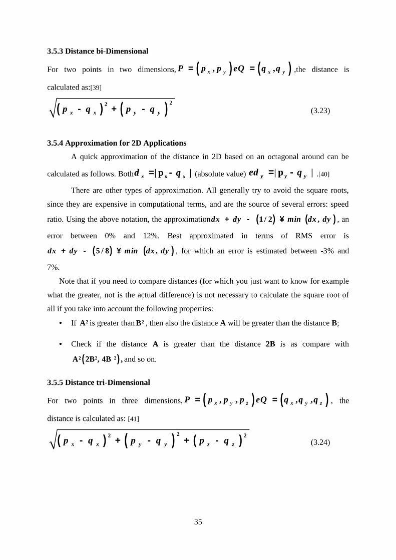
3.5.3 Distance bi-Dimensional
For two points in two dimensions, , ,x y x yP p p eQ q q ,the distance is
calculated as:[39]
22x x y yp q p q (3.23)
3.5.4 Approximation for 2D Applications
A quick approximation of the distance in 2D based on an octagonal around can be
calculated as follows. Both x| p |x xd q (absolute value) | p |y y yed q .[40]
There are other types of approximation. All generally try to avoid the square roots,
since they are expensive in computational terms, and are the source of several errors: speed
ratio. Using the above notation, the approximation 1 / 2 ,dx dy min dx dy , an
error between 0% and 12%. Best approximated in terms of RMS error is
5 / 8 ,dx dy min dx dy , for which an error is estimated between -3% and
7%.
Note that if you need to compare distances (for which you just want to know for example
what the greater, not is the actual difference) is not necessary to calculate the square root of
all if you take into account the following properties:
If A² is greater than B² , then also the distance A will be greater than the distance B;
Check if the distance A is greater than the distance 2B is as compare with
A² 2B², 4B ² , and so on.
3.5.5 Distance tri-Dimensional
For two points in three dimensions, , , , ,x y z x y zP p p p eQ q q q , the
distance is calculated as: [41]
22 2
x x y y z zp q p q p q (3.24)

36
3.6 Fast Pixel Based Matching Using Edge Detection (FPBM)
The recognition of the contours (edge detection) is used for the purpose of marking the
points of a digital image in which the light intensity changes abruptly. Abrupt changes of the
properties of an image are usually a symptom of events or major changes of the physical
world where images are the representation. These changes can be for example: discontinuity
of depth discontinuities in the surface, changing the properties of materials, and variations in
lighting conditions from the surrounding environment. The edge detection is a research field
of image processing and computer vision, particularly the branch of feature recognition
(feature extraction).
The operation of edge detection generates images containing much less information
than the original, because it eliminates most of the details are not relevant for the purpose of
identifying the boundaries, while preserving the essential information to describe the shape
and structural characteristics and geometric of the objects represented.[42]
There are many ways to recognize the outlines, but most can be grouped into two
categories: methods based on research (search-based) and methods zero (zero-crossing).
Methods based on research recognize the contours of trying the maxima and minima of the
first order derivative of the image, usually looking for the direction in which we have the
maximum local gradient. The methods seek the zero-crossing points at which the derivative of
the second order passes through zero, usually the Laplacian function or a differential
expression of a non-linear function. [43]
Figure 3.5: Edge detection. [43]

37
3.6.1 Properties and the Contours
The contours can be dependent on the point of observation, may change when the
change of the observation point, reflecting the arrangement and geometric configuration of the
surrounding environment, such as, objects that hinder one another, or they can be independent
from the point of observation, when reflect intrinsic properties of the objects themselves, such
as signs on surfaces or geometric shapes of the surfaces of objects. In two or more dimensions
must take into consideration the effects of perspective. [42]
A typical contour could be, for example, the boundary between an area of red colour
and a yellow, or a line with a thickness of a few pixels and a different colour compared to a
uniformly colour background. In the latter case, the contours are precisely two, one for each
side of the line.
The contours play a very important role in many applications of computer vision, even
if, in recent times, in this field have been made substantial progress also using other
approaches, which do not use the recognition of contours as a preliminary step of the
processing.
3.6.2 Simplified Mathematical Model
In real images the contours are almost never net, but they are usually suffering from one
or more of the following distortions:[44]
Focus imperfect because of the depth of field is not infinite optics of the instrument of
acquisition.
Presence of soft shadow created by non-point sources of illumination.
Gray scales which are made with rounded corners.
Effects of specular or antireflection in the vicinity of the edges.
The model illustrated here, although not perfect, it has a function error erf that can be
used to create a mathematical model of the effects of the blurs sufficient accurate to describe
many practical applications. An image f with a one-dimensional contour positioned exactly
in 0 can be represented then by the following function:
12 2
r ll
I I xf x erf I
(3.25)

38
3.6.3 Calculation of the First Derivative
Many algorithms for the recognition of contours operate on the first order derivative of
the light intensity - which corresponds to the gradient of the intensity of the initial image.
Based on this output you can go in search of the peak values of the gradient of intensity.[45]
If I x represent the intensity of pixel x, and I x denotes the derivative (gradient
intensity) to the pixel x, we get:
I 1 2. 1 0.I 1 2. 1x I x x I x (3.26)
3.6.4 Calculation of the Second Derivative
Other operator for edge detection is based on calculation of the second derivative of
the intensity, which roughly corresponds to the rate of change of the gradient. In the ideal case
- in which the intensity varies in a continuous manner - the second derivative vanishes at the
points of maximum gradient.[45] This method, however, works well only if the image is
represented in a suitable scale. As explained before, a line corresponds to a double contour,
and then you will have a gradient of intensity on one side of the line, immediately followed by
a gradient of opposite value on the opposite side. For this reason it can be expected to have
large variations in the gradient images containing lines.
If I x is the intensity value at the point x and I" x is the second derivative at the
point x, then the following relation holds:
" 1. 1 – 2. 1. 1I x I x I x I x (3.27)
3.6.5 Operators for Edge Detection
Operators of the first order : Roberts, Prewitt , Sobel
Operators of the second order: Marr - Hildreth, the zero crossing of the derivative of
the second order in the direction of the gradient (zero crossing).
Currently the Canny algorithms - and its variants - are the most used method for the
recognition of contours. None of the numerous other subsequently proposed methods has so
far proved more effective, except in very specific applications. In his original work, Canny set
out to find a filter that would eliminate the noise in the image ( .i e ., a smoothing filter) filter
that could be well approximated by a Gaussian kernel of the first order.

39
Canny also introduced the concept of non - maximum suppression, namely the
assumption that the points of the contours are those in which the gradient reaches the
maximum value in the estimated direction of the gradient. The search for non - maximum in a
grid of points can be implemented by calculating the gradient direction with the first
derivative, rounding the direction found in multiples of 45 °, and finally comparing with the
values of amplitude of the gradient in the direction calculated.
A more accurate method to research the contours with higher accuracy of the pixels is
to use the following expression differential to find the zero crossing of the derivative of the
second order in the direction of the gradient (Lindenberg 1998).
2 22 0x xx x y xy y yyL L L L L L L (3.28)
That satisfies the equality sign of the derivative of the third order in the same direction:
3 2 2 33 3 0x xxx x y xxy x y xyy y yyyL L L L L L L L L L (3.29)
Where x y yyyL L L represent the partial derivatives calculated in a spatial representation of
multi-scale (scale-space) Lobtained by blurring the original image with a Gaussian kernel.
With this procedure, the contours will be obtained automatically as continuous curves with
sub-pixel accuracy. Even thresholding with hysteresis can be applied to sub-pixel segments.

40
3.7 Summary
PCA is a mathematical decomposition of variance, and it will extract factors
accounting for many sources of variance. This chapter describes the basic steps of
PCAalgorithm. The derivation of basic parameters of PCA has been explained. The application of the
derived algorithms to the fingerprint images is considered.

41
4. DESIGN OF FINGERPRINT RECOGNITION SYSTEM
4.1. Overview
In this chapter the design of finger recognition system has been performed. For feature
extraction of fingerprint images the Principal Component Analysis (PCA) is used. For
comparative analysis the Fast Pixel Based Matching (FPBM) were used. The basic structure
of fingerprint recognition system is given. The flowcharts of the designed program have been
described. The Euclidean distance has been applied for classification of the fingerprints.
4.2 General Structure of Fingerprint Recognition
The general structure of the fingerprint recognition program is shown in Figure 4.1 the
inputs of the system are fingerprint images. These images are accumulated in image database.
After database creation, the used image is sent to the feature extraction block. In these thesis
two methods- PCA and FPBM are used for feature extraction. These methods are applied to
obtain the principal components of fingerprint images. Using these feature the classification
of the images are carried out. The decision is made if there is matching in the classification
block.
Figure 4.1: General Structure of the program.

42
4.3 Flowcharts of Feature Extraction Methods
The two methods (PCA, FPBM) were used for feature extraction during simulation.
Each of them was explained in chapter 3, and the flowcharts of these methods were given in
this section.
All image data are represented by greyscale values. Principles Component Analysis
(PCA) are used for feature extraction. Some operations should be done for pre-processing of
the images. Figure 4.2 show converting all images from 2D to 1D. Store 1D images in vector
called T. Converting from 2D vector to 1D vector is done using reshape function.
Figure 4.2: Flowchart of converting 2D images to 1D.
Figure 4.3 shows the computing for mean, deviation and eigenvector. After reading T
vector from previous function, compute the mean image. The mean image means the average
for all images. After that, compute the deviation for all images (each one alone) from the
mean value of image. The deviation means the difference between the image and the mean
value of image. Now, we need to compute the surrogate for covariance matrix. Finally,
computation of the eigenvector is performed by multiplication of the deviation an image and
surrogate matrix.

43
Figure 4.3: Flowchart for computing eigenvector.

44
Figure 4.4 shows the steps for extracting the PCA feature from test image to make
recognition.
PCA feature are:-
Reshape tested image to 1D image vector.
Compute the deviation for tested image and the mean image.
Projecting the test image into fingerprint space.
Figure 4.4: Flowchart for extracting of PCA feature for tested image.
Finally computed and store Euclidean distances in a vector by subtracting of projected
image from projected test image then,
1. Applying norm function.
2. Square the result, the store it in that vector see Figure 4.5.
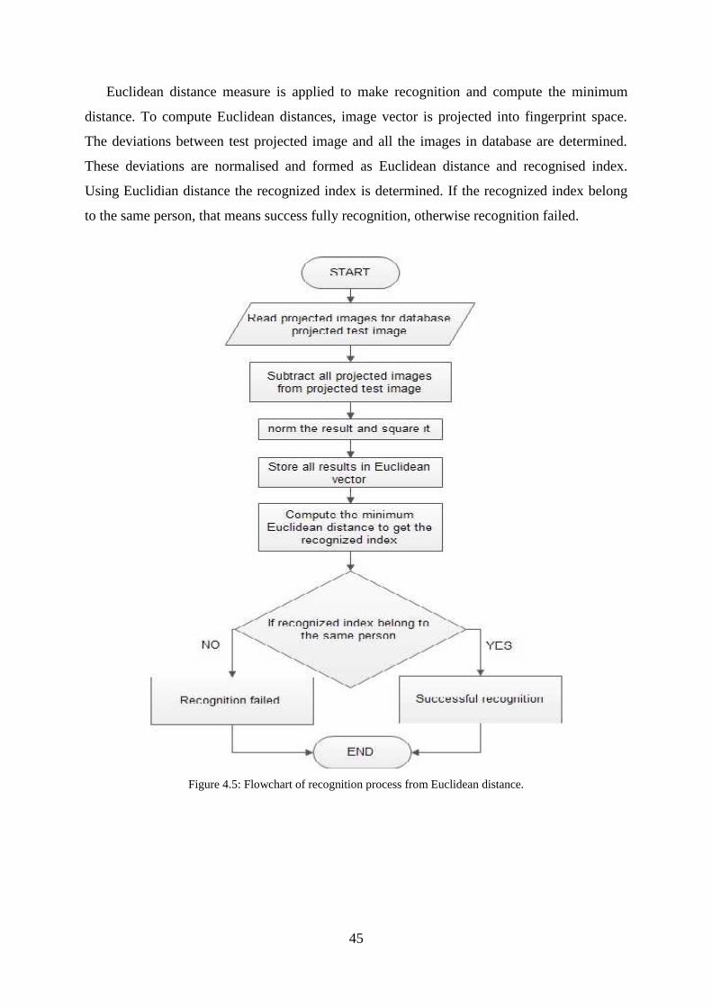
45
Euclidean distance measure is applied to make recognition and compute the minimum
distance. To compute Euclidean distances, image vector is projected into fingerprint space.
The deviations between test projected image and all the images in database are determined.
These deviations are normalised and formed as Euclidean distance and recognised index.
Using Euclidian distance the recognized index is determined. If the recognized index belong
to the same person, that means success fully recognition, otherwise recognition failed.
Figure 4.5: Flowchart of recognition process from Euclidean distance.

46
Figure 4.6 shows the steps for recognition process using the second FPBMalgorithm.
FPBM algorithm depended on comparing of white and black points of two images.By
applying edge (image, ‘prewitt’) function with 'prewitt' property, the image converted to black
colour and all edged points converted to white colour. Matching percentage in this algorithm
depends on the total data and matched data. The total data means number of white points in
tested image. Matched data means, the number of white points that matched between tested
image and recognized image.
Figure 4.6: Flowchart of FPBM.
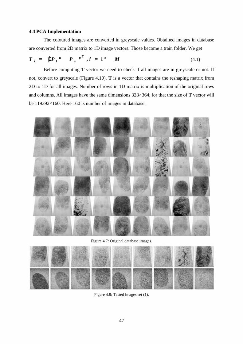
47
4.4 PCA Implementation
The coloured images are converted in greyscale values. Obtained images in database
are converted from 2D matrix to 1D image vectors. Those become a train folder. We getT
1 1,i mT P P i M (4.1)
Before computing T vector we need to check if all images are in greyscale or not. If
not, convert to greyscale (Figure 4.10). T is a vector that contains the reshaping matrix from
2D to 1D for all images. Number of rows in 1D matrix is multiplication of the original rows
and columns. All images have the same dimensions 328×364, for that the size of T vector will
be 119392×160. Here 160 is number of images in database.
Figure 4.7: Original database images.
Figure 4.8: Tested images set (1).

48
Figure 4.9: Tested images set (2).
Figure 4.10: Convert from RGB to grayscale.
Now calculate the mean of training image, by summation for all Ti Equation (4.1)
according to equation:
M
iiT
Mm
1
1(4.2)
Size of the mean image matrix for the same number of images in database will be 119392×1,
because of division by the number of images (160) in database. After that compute the
deviation of each image from the mean image according to this formula:
–i iA T m (4.3)

49
The size of the deviation vector equals the size of T vector. It is necessary to get the
surrogate of covariance matrixC which is equal to A A'C . The surrogate L is equal to
A A'L . The size of surrogate is 160 × 160 because of the size of A' = 160×119392 and
the size of A equals to 119392×160.
Computing of diagonal elements of surrogate will give the Eigenvectors for both of
covariance and surrogate matrix. These Eigenvectors are scaled, so that it would be greater
than 1. If ( , 1D i i ) add V to Eigenvectors. In this case the size of Eigenvectors 160×159
because of D (1, 1) is less than 1.
Now, calculations for Eigenvectors of covariance matrix are ready. Eigenvectors are
the reseals of multiplication between the deviation vector and diagonal elements of vector.
The sizes of them are 119392×160 and 160×159 respectively. So the size of Eigenvectors is
119392×159.
To classify the recognition results, it is necessary to compute Euclidean distances
between projected test image and projected database image. For database image, projection of
centred images into fingerprint space can be calculated by multiplication of the transpose of
eigenvectors and deviation of all images. Its size equals to 159×159 because of transpose of
eigenvectors size is equal to 159×119392. The size of the deviation vector is 119392×160 but
because of in eigenvectors there are 159 rows only the size of projected vector will be equal to
159×159. That is they will be multiplied with 159 columns of deviation vector.
Nextwe need to compute PCA feature of projected test images.
1. Convert test image to 1D vector.
2. Compute the deviation of tested image from the mean image.
3. Compute of projected test image by multiplication of transpose of Eigenvectors with
the deviation of tested image.
To generate Euclidean distance vector, compute the difference of projected tested image
from all projected database images. Then compute the norm and the square for these
computed differences. Next compute the minimum Euclidean distance and its index. If this
index belong to the same person then the tested image belong to the same image. Then the
image is recognized successfully otherwise, no recognition.

50
4.5 Implementation for FPBM (Fast Pixel Based Matching)
This is a traditional method to compute matching percentage between two images. In
this thesis, 78% used as the minimum percentage to say those images are matched. Before
starting implementation of FPBM, check if the two images are greyscale? If not, convert to
greyscale by using rgb2gray (image) function (see Figure 4.10).
To compute the percentage of matching uses this formula:
.
.
R 100Matched data
Total data
; where: (4.3)
1. R: is the percentage matching.
2. Total data: all white points in tested image.
3. Matched data: all white points that matched between the two images.
To compute the white and black points of any image, use edge (image, 'priwitt') function
see Figure 4.11, if the point of edged point value equals 1; that means it is white point.
Otherwise, it is black point. To compute the matched points in the two images, use the same
resulted for edge function. If a point of the first edged image and the second edged image
equal to 1, that means they are match with white colour. So increased the matched data and
complete.
Figure 4.11: Effect of edge (image, ‘prewitt’).
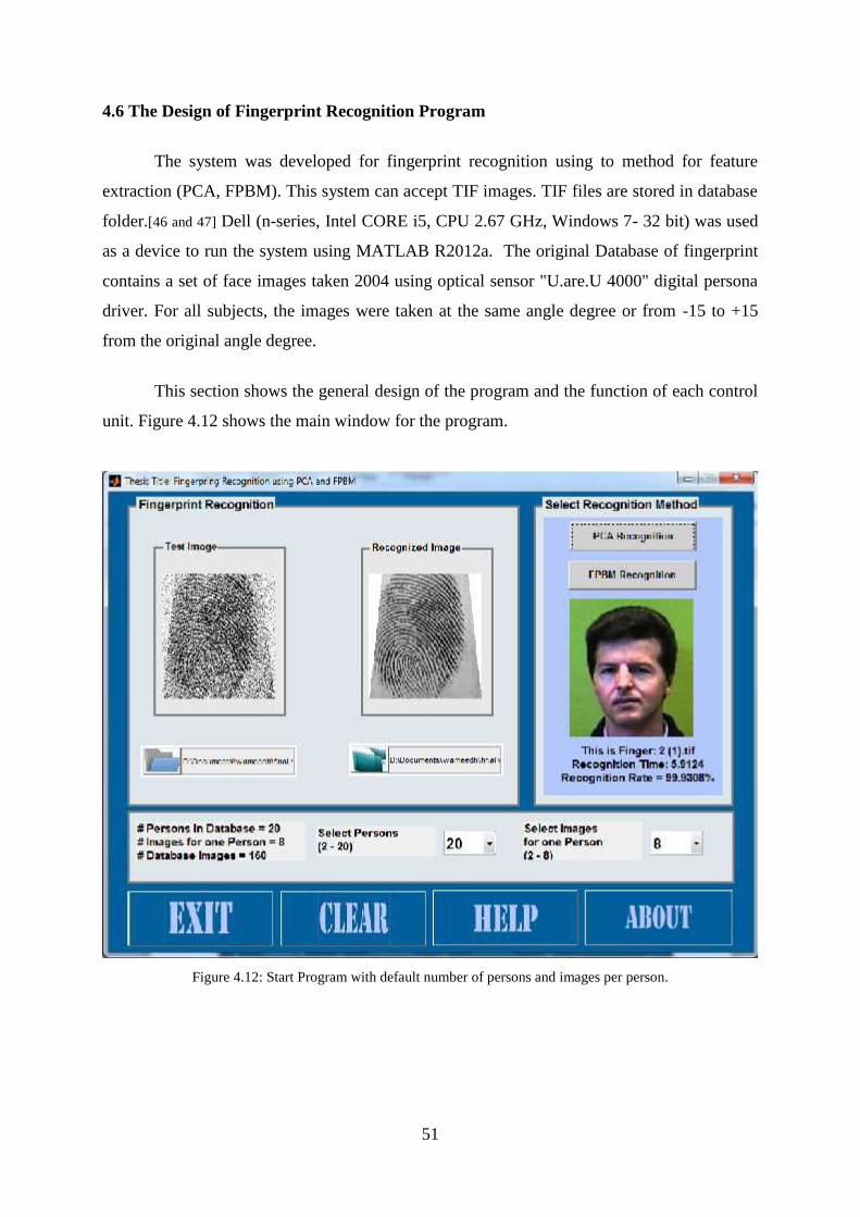
51
4.6 The Design of Fingerprint Recognition Program
The system was developed for fingerprint recognition using to method for feature
extraction (PCA, FPBM). This system can accept TIF images. TIF files are stored in database
folder.[46 and 47] Dell (n-series, Intel CORE i5, CPU 2.67 GHz, Windows 7- 32 bit) was used
as a device to run the system using MATLAB R2012a. The original Database of fingerprint
contains a set of face images taken 2004 using optical sensor "U.are.U 4000" digital persona
driver. For all subjects, the images were taken at the same angle degree or from -15 to +15
from the original angle degree.
This section shows the general design of the program and the function of each control
unit. Figure 4.12 shows the main window for the program.
Figure 4.12: Start Program with default number of persons and images per person.

52
Select tested fingerprint image from test folder by clicking the selection image button.
Figure 4.13: Input test image by selection from that button.
Select the database path by clicking the database button. The program is designed to
prevent all bugs. So, you automatically select the path of database and the path of tested
image.
Figure 4.14: Selection of database folder from that button.

53
To determine the database path, select a number from the two popup menus Figure
4.15 to select the number of persons in the database, use first popup menu. To select the
number of images per person in the database, use second popup menu.
Figure 4.15: Creation database, number of person (2-20), number of images per person (2-8)
After all previous steps; start recognition without problems. There are two methods
used in this program. PCA and FPBM and each method have a special button to make
recognition using selected one.
Figure 4.16: Selection of recognition methods (PCA, FPBM).
This part shows the results. If the recognition was successful, the image for that person
is shown. The time was spent in recognition process also shown. The recognition rate between
the two images is also shown as a result.
Figure 4.17: Results with successful recognition.

54
The second type is not recognized results. This will show as unknown person and also
“Sorry Not Matching” statement as result.
Figure 4.18a: Results with fail recognition.
Figure 4.18b: Image when recognition is failed.
Helpful buttons: CLEAR button for clear all inputs and outputs. HELP button shows
how algorithms running step by step, ABOUT button shows information about program
designer.
Figure 4.19: Helpful buttons: CLEAR, HELP, ABOUT and EXIT.

55
4.7 Tested Samples
Below three simulation results obtained from the program is given:
⁻ First sample
Figure 4.20: Snapshot for first sample.

56
Next tables show information about original images in database folder and tested folder.
Table 4.1: Information about images and matrices in database in first test.
Information about images in database
Extension of images TIF
Size of images 328 × 364
Colour of images Grayscale
Number of persons in database 10
Number of images per person 5
Number of images in database 50
Size of (T) vector 119392 × 50
Size of The mean (m) 119392 × 1
Size of The deviation (A) 119392 × 50
Size of Eigenvectors 119392 × 49
Size of projected images 49 × 49
Size of Euclidean distances 1 × 49
Minimum Euclidean distance 2.8904e+16
Table 4.2: Information about tested image in first test.
Information tested image
Extension of image TIF
Size of image 328 × 364
Colour of image Grayscale
Size of (T) vector 119392 × 1
Size of The mean (m) 119392 × 1
Size of The deviation (A) 119392 × 1
Size of projected test image 49 × 1
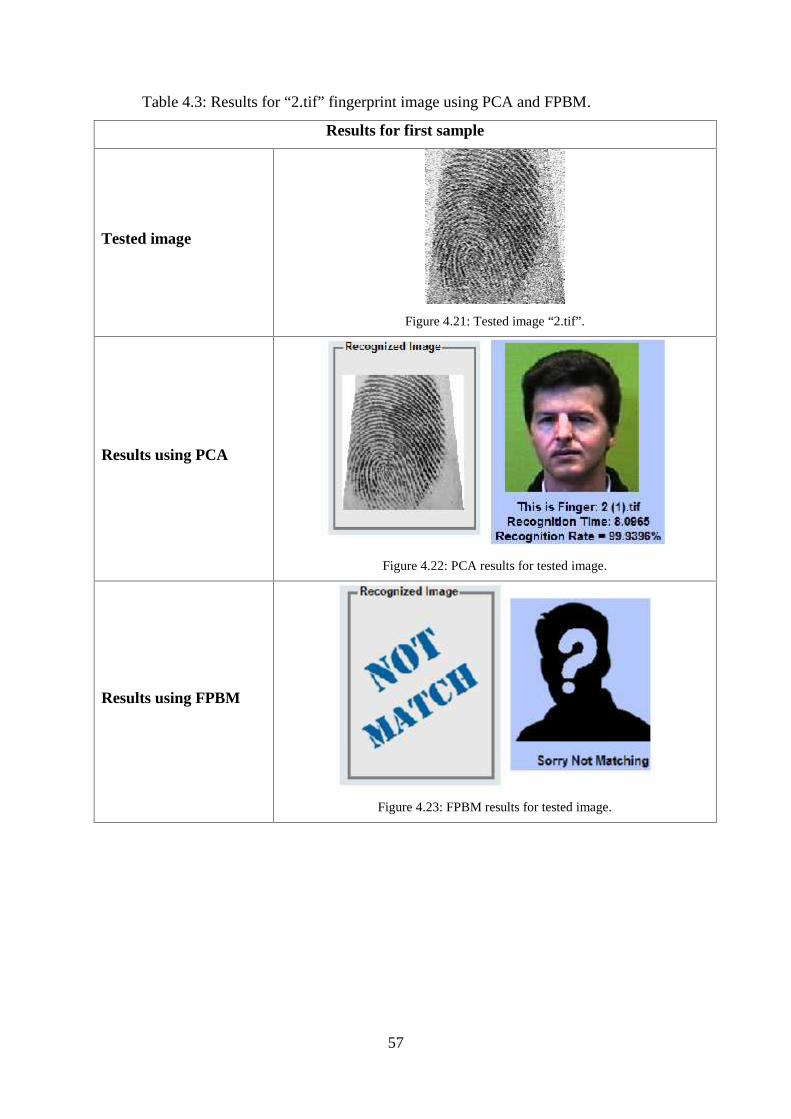
57
Table 4.3: Results for “2.tif” fingerprint image using PCA and FPBM.
Results for first sample
Tested image
Figure 4.21: Tested image “2.tif”.
Results using PCA
Figure 4.22: PCA results for tested image.
Results using FPBM
Figure 4.23: FPBM results for tested image.

58
- Second sample
Figure 4.24: Snapshot for second sample.

59
Next tables show information about original images in database folder and tested folder.
Table 4.4: Information about images and matrices in database in second test.
Information about images in database
Extension of images TIF
Size of images 328 × 364
Colour of images Grayscale
Number of persons in database 10
Number of images per person 5
Number of images in database 50
Size of (T) vector 119392 × 160
Size of The mean (m) 119392 × 1
Size of The deviation (A) 119392 × 160
Size of Eigenvectors 119392 × 159
Size of projected images 159 × 159
Size of Euclidean distances 1 × 159
Minimum Euclidean distance 8.2239e+16
Table 4.5: Information about tested image in second test.
Information tested image
Extension of image TIF
Size of image 328 × 364
Colour of image Grayscale
Size of (T) vector 119392 × 1
Size of The mean (m) 119392 × 1
Size of The deviation (A) 119392 × 1
Size of projected test image 159 × 1

60
Table 4.6: Results for “3.tif” fingerprint image using PCA and FPBM.
Results for Second sample
Tested image
Figure 4.25: Tested image “3.tif”.
Results using PCA
Figure 4.26: PCA results for tested image.
Results using FPBM
Figure 4.27: FPBM results for tested image.

61
- Third sample
Figure 4.28: Snapshot for third sample.

62
Next tables show information about original images in database folder and tested folder.
Table 4.7: Information about images and matrices in database in third test.
Information about images in database
Extension of images TIF
Size of images 328 × 364
Colour of images Grayscale
Number of persons in database 20
Number of images per person 8
Number of images in database 160
Size of (T) vector 119392 × 160
Size of The mean (m) 119392 × 1
Size of The deviation (A) 119392 × 160
Size of Eigenvectors 119392 × 159
Size of projected images 159 × 159
Size of Euclidean distances 1 × 159
Minimum Euclidean distance 7.1559e+16
Table 4.8: Information about tested image in third test.
Information tested image
Extension of image TIF
Size of image 328 × 364
Colour of image Grayscale
Size of (T) vector 119392 × 1
Size of The mean (m) 119392 × 1
Size of The deviation (A) 119392 × 1
Size of projected test image 159 × 1
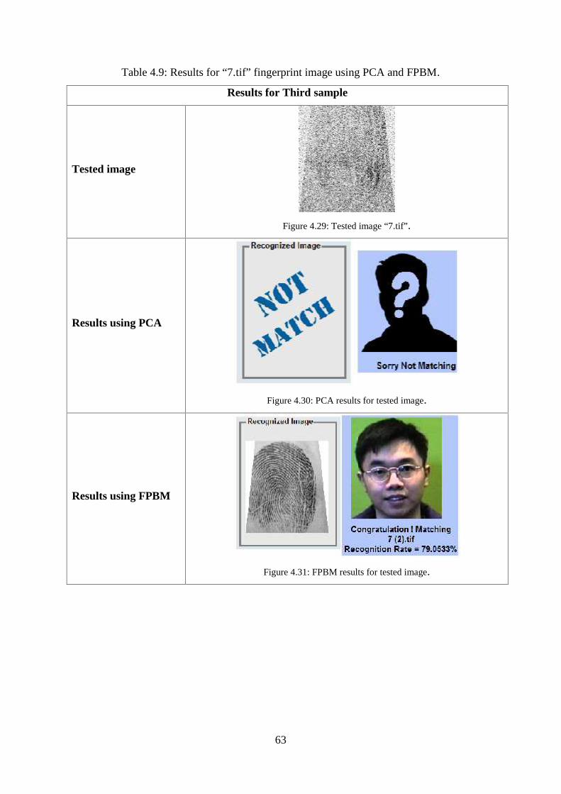
63
Table 4.9: Results for “7.tif” fingerprint image using PCA and FPBM.
Results for Third sample
Tested image
Figure 4.29: Tested image “7.tif”.
Results using PCA
Figure 4.30: PCA results for tested image.
Results using FPBM
Figure 4.31: FPBM results for tested image.

64
4.8 Results
The simulation results of the fingerprint recognition system are obtained using PCA
feature extraction method. For comparative analysis FPBM technique was used. The
simulations are performed in two stages. In first stage the noisy tested images, in second stage
tested images without noisy are considered for recognition. For each experiment the
Recognition Rate was obtained. The results are given in Table 4.10.
In first experiment 80 images of 10 persons are taken. In image database each person
has 8 different images. The number of noisy tested images that used in this experiment was
10. Using PCA 7 images was recognized successfully and recognition rate was obtained as
70%. Using FPBM 6 images was recognized and recognition rate was obtained 60%.
In the second experiment, 120 images of 15 persons are taken. In database each person
has 8 different images. Number of noisy tested images that is used in this experiment was 15.
Using PCA 10 images was recognized successfully with recognition accuracy66.7%. Using
FPBM 7 images was recognized successfully with recognition accuracy 46.7%.
In the third experiment, 160 images are taken. These images are belonging to 20
persons and each person has 8 different images. The number of noisy tested images that are
used in this experiment was 20. Using PCA 13 images was recognized successfully with
recognition accuracy 65%. Using FPBM 11 images was recognized successfully with
recognition accuracy 55%.
Table 4.10: Recognition rates of the system for noisy tested images.
Tested set image is same for all experiments
Number
of
persons
Number
of tested
images
Number of
images in
database
PCA FPBM
R.R E.R R.R E.R
10 30 80 70% 30% 60% 40%
15 15 120 66.7% 33.3% 46.7% 53.3%
20 20 160 65% 35% 55% 45%

65
In next stage the simulation results were obtained using tested images (without noisy)
from second image data set. Table 4.11 shows simulation results of fingerprint recognition
system using PCA and FPBM algorithms.
In the first experiment, 24 images of 6 persons are taken. In image database each
person has 4 different images. Number of tested images that used in this experiment is 6.
Using PCA 6 images was recognized successfully and recognition rate was 100%. Using
FPBM 4 images was recognized successfully and recognition rate was 66.7%.
In the second experiment, 52 images are taken. In database these images are belonging
to 13 persons. Each person has 4 different images. Number of tested images that is used in
this experiment was 13. Using PCA 12 images was recognized successfully with recognition
accuracy 93%. Using FPBM 10 images was recognized successfully with recognition
accuracy 76.9%.
In the third experiment, 68 images are taken. These images are belonging to 17
persons and each person has 4 different images. Number of tested images that are used in this
experiment was 34. Using PCA 31 images was recognized successfully with recognition
accuracy 91.1%. Using FPBM 25 images was recognized successfully with recognition
accuracy 73.5%.
The simulation results demonstrate the efficiency of using of PCA method over other
methods in fingerprint recognition.
Table 4.11: Recognition rates of the system for not noisy tested images.
Tested set image is same for all experiments
Number
of
persons
Number
of tested
images
Number
of images
in
database
PCA FPBM
R.R E.R R.R E.R
6 6 24 100 % 0 % 66.7 % 33.3 %
13 13 52 93% 7 % 76.9 % 23.1 %
17 34 68 91.1% 8.9 % 73.5 % 26.5 %
66
5. CONCLUSIONIn this thesis fingerprint Recognition system was designed using MATLAB program.
Two different feature extraction methods (PCA and FPBM) and Euclidean distance
classification were used to develop the system. The structure of fingerprint recognition system
was designed. The used feature extraction methods are described in detail. Using PCA and
FPBM the design of fingerprint recognition system has been performed.
The designed system was tested with two types of fingerprint image data sets.In the first
data base the fingerprint imagesdid not have noise and in second database fingerprint images
havenoise. The results were recorded as recognition rate.
Simulation of fingerprint recognition system has been performed for two kinds of test
images: noisy and without noisy cases. Simulation results for FPBM method have average
recognition rate for noisy fingerprint images 53.9%. For non-noisy fingerprint images the
average recognition rate was 72.4%. The best recognition rate using FPBM and with noisy
fingerprint images was 60%. The best recognition rate using FPBM without noisy fingerprint
images was 76.9%. That means, the FPBM method is useful for non-noisy and not useful for
noisy fingerprint images.
Simulation results for PCA method have average recognition rate for noisy fingerprint
images 67.2%. For non-noisy fingerprint images the average recognition rate was 94.7%. The
best recognition rate using PCA and with noisy fingerprint images was 70%. The best
recognition rate using PCA without noisy fingerprint images was 100%. That means, the PCA
method is useful for noisy fingerprint images and useful for non-noisy fingerprint images.
Fingerprint recognition system was designed using MATLAB 2012.a package.
MATLAB is a good environment to develop different feature extraction methods using GUI.
GUIDE (GUI development environment) provides tools for designing GUIs for custom
applications. GUIDE then automatically generates the MATLAB code for constructing the
GUI, which you can modify to program the behaviour of an application.For classification
purpose the Euclidean distance algorithm is used.
67
REFERENCES
[1] Lenchik, L., Rogers, L. F., Delmas, P. D., &Genant, H. K. (2004). Diagnosis of
osteoporotic vertebral fractures: importance of recognition and description by
radiologists. American Journal of Roentgenology, 183(4), 949-958.
[2] Zdobnov, E. M., &Apweiler, R. (2001). InterProScan–an integration platform for the
signature-recognition methods in InterPro. Bioinformatics, 17(9), 847-848.
[3] Snelick, R., Indovina, M., Yen, J., & Mink, A. (2003, November). Multimodal
biometrics: issues in design and testing. In Proceedings of the 5th international
conference on Multimodal interfaces (pp. 68-72). ACM.
[4] Jain, A. K., Dass, S. C., &Nandakumar, K. (2004). Soft biometric traits for personal
recognition systems. In Biometric Authentication (pp. 731-738). Springer Berlin
Heidelberg.
[5] Jain, A. K., Ross, A., &Pankanti, S. (2006). Biometrics: a tool for information
security. Information Forensics and Security, IEEE Transactions on, 1(2), 125-143.
[6] Huopio, S. (1988). Biometric identification. Eye, 3, 1.
http://www.tml.tkk.fi/Opinnot/Tik-110.501/1998/papers/12biometric/biometric.htm
[7] Kolb, H., Fernandez, E., & Nelson, R. (2005). Gross anatomy of the eye.
http://www.ncbi.nlm.nih.gov/books/NBK11534/
[8] Kroeker, K. L. (2009). Face recognition breakthrough. Communications of the
ACM, 52(8), 18-19.
http://dl.acm.org/citation.cfm?id=1536623
[9] Fitch, W. T., & Hauser, M. D. (2003). Unpacking “honesty”: vertebrate vocal production
and the evolution of acoustic signals. In Acoustic communication(pp. 65-137). Springer
New York.
[10] Jiang, X., &Yau, W. Y. (2000). Fingerprint minutiae matching based on the local and
global structures. In on Proceedings of 15th International Conference Pattern Recognition,
2000. (Vol. 2, pp. 1038-1041).IEEE.

68
[11] Merkle, R. C. (1990, January). A certified digital signature. In Proceedings ofAdvances
in Cryptology—CRYPTO’89 (pp. 218-238). Springer New York.
[12] Rohs, R., West, S. M., Sosinsky, A., Liu, P., Mann, R. S., &Honig, B. (2009). The role
of DNA shape in protein–DNA recognition. Nature, 461(7268), 1248-1253.
[13] Yun, Y. W. (2002). The ‘123’of biometric technology. Synthesis Journal, 2002.
http://www.cp.su.ac.th/~rawitat/teaching/forensicit06/coursefiles/files/biometric.pdf
[14] Wold, S. (1976). Pattern recognition by means of disjoint principal components
models. Pattern recognition, 8(3), 127-139.
[15] Prabhakar, S. (2001). Fingerprint classification and matching using a
filterbank(Doctoral dissertation, Michigan State University).
http://biometrics.cse.msu.edu/Publications/Thesis/SalilPrabhakar_FpMatching
Filterbank_PhD01.pdf
[16] Camenisch, J. (2000). Efficient anonymous fingerprinting with group signatures.
In Advances in Cryptology—ASIACRYPT 2000 (pp. 415-428). Springer Berlin
Heidelberg.
[17] Cole, S. A. (2009). Suspect identities: A history of fingerprinting and criminal
identification. Harvard University Press.
[18] Kawagoe, M., &Tojo, A. (1984). Fingerprint pattern classification. Pattern
Recognition, 17(3), 295-303.
http://www.sciencedirect.com/science/article/pii/0031320384900797
[19] Hong, L., Wan, Y., & Jain, A. (1998). Fingerprint image enhancement: algorithm and
performance evaluation. Pattern Analysis and Machine Intelligence, IEEE Transactions
on, 20(8), 777-789.
[20] Chong, M., Tan, H. N., Jun, L., & Gay, R. K. (1997). Geometric framework for
fingerprint image classification. Pattern Recognition, 30(9), 1475-1488.
http://www.sciencedirect.com/science/article/pii/S0031320396001781

69
[21] Maio, D., & Jain, A. K. (2009). Handbook of fingerprint recognition.springer.
[22] Harris, T. (2002). How fingerprint scanners work. HowStuffWorks.com.
http://www.armchairpatriot.com/How%20Stuff%20Works/How%20Fingerprint%20
Scanners%20Wo.pdf
[23] Secretary slaves, fingerprint reader, King Saud University, May 13, 2009, Riyadh.
[24] Ratha, N. K., Chen, S., & Jain, A. K. (1995). Adaptive flow orientation-based feature
extraction in fingerprint images. Pattern Recognition, 28(11), 1657-1672.
http://www.sciencedirect.com/science/article/pii/0031320395000393
[25] Maltoni, D., Maio, D., Jain, A. K., &Prabhakar, S. (2003). Introduction (pp. 1-52).
Springer New York.
http://link.springer.com/chapter/10.1007/0-387-21587-5_1#page-1
[26] Ross, A., Reisman, J., & Jain, A. (2006). Fingerprint matching using feature space
correlation. In Biometric Authentication (pp. 48-57).Springer Berlin Heidelberg.
http://link.springer.com/chapter/10.1007/3-540-47917-1_6
[27] Cappelli, R., Maio, D., &Maltoni, D. (2004, June). SFinGe: an approach to synthetic
fingerprint generation. In International Workshop on Biometric Technologies
(BT2004) (pp. 147-154).
http://math.la.asu.edu/~dieter/courses/Math_Modeling_2013/Cappelli_2004.pdf
[28] Takeuchi, H., Umezaki, T., Matsumoto, N., &Hirabayashi, K. (2007). Evaluation of
low‐quality images and imaging enhancement methods for fingerprint
verification. Electronics and Communications in Japan (Part III: Fundamental
Electronic Science), 90(10), 40-53.
[29] Smith, L. I. (2002). A tutorial on principal components analysis. Cornell University,
USA, 51, 52.
http://www.ce.yildiz.edu.tr/personal/songul/file/1097/principal_components.pdf

70
[30] Ratha, N., &Bolle, R. (Eds.). (2004). Automatic fingerprint recognition systems.
Springer.
[31] Jea, T. Y., &Govindaraju, V. (2005). A minutia-based partial fingerprint recognition
system. Pattern Recognition, 38(10), 1672-1684.
http://www.sciencedirect.com/science/article/pii/S0031320305001445
[32] Wold, S., Esbensen, K., &Geladi, P. (1987). Principal component
analysis.Chemometrics and intelligent laboratory systems, 2(1), 37-52.
http://www.sciencedirect.com/science/article/pii/0169743987800849
[33] Bazen, A. M., &Gerez, S. H. (2000, November). Directional field computation for
fingerprints based on the principal component analysis of local gradients.
InProceedings of ProRISC2000, 11th Annual Workshop on Circuits, Systems and
Signal Processing (pp. 215-222). Veldhoven, the Netherlands.
[34] Chen, L. F., Liao, H. Y. M., Ko, M. T., Lin, J. C., & Yu, G. J. (2000). A new LDA-
based face recognition system which can solve the small sample size problem. Pattern
recognition, 33(10), 1713-1726.
http://www.sciencedirect.com/science/article/pii/S0031320399001399
[35] Zhao, W., Krishnaswamy, A., Chellappa, R., Swets, D. L., &Weng, J. (1998).
Discriminant analysis of principal components for face recognition. In Face
Recognition (pp. 73-85). Springer Berlin Heidelberg.
http://link.springer.com/chapter/10.1007/978-3-642-72201-1_4#page-1
[36] Saito, T., &Toriwaki, J. I. (1994). New algorithms for euclidean distance transformation
of an-dimensional digitized picture with applications.Pattern recognition, 27(11), 1551-
1565. http://www.sciencedirect.com/science/article/pii/0031320394901333
[37] Danielsson, P. E. (1980). Euclidean distance mapping. Computer Graphics and image
processing, 14(3), 227-248.
http://www.sciencedirect.com/science/article/pii/0146664X80900544

71
[38] Wang, L., Zhang, Y., & Feng, J. (2005). On the Euclidean distance of images.Pattern
Analysis and Machine Intelligence, IEEE Transactions on, 27(8), 1334-1339.
[39] Kuntz, P., Snyers, D., &Layzell, P. (1999). A stochastic heuristic for visualising graph
clusters in a bi-dimensional space prior to partitioning. Journal of Heuristics, 5(3),
327-351.http://link.springer.com/article/10.1023/A:1009665701840#page-1
[40] Perdew, J. P., Chevary, J. A., Vosko, S. H., Jackson, K. A., Pederson, M. R., Singh, D.
J., &Fiolhais, C. (1992). Atoms, molecules, solids, and surfaces: Applications of the
generalized gradient approximation for exchange and correlation. Physical Review
B, 46(11), 6671. http://prb.aps.org/abstract/PRB/v46/i11/p6671_1
[41] Gonzalez-Herrera, A., & Zapatero, J. (2008). Tri-dimensional numerical modelling of
plasticity induced fatigue crack closure. Engineering Fracture Mechanics, 75(15),
4513-4528.http://www.sciencedirect.com/science/article/pii/S001379440800115X
[42] Maio, D., &Maltoni, D. (1997). Direct gray-scale minutiae detection in
fingerprints. Pattern Analysis and Machine Intelligence, IEEE Transactions on,19(1),
27-40.
[43] Marr, D., &Hildreth, E. (1980). Theory of edge detection. Proceedings of the Royal
Society of London. Series B. Biological Sciences, 207(1167), 187-217.
http://rspb.royalsocietypublishing.org/content/207/1167/187.short
[44] Shen, J., & Chan, T. F. (2002). Mathematical models for local nontexture
inpaintings. SIAM Journal on Applied Mathematics, 62(3), 1019-1043.
http://epubs.siam.org/doi/abs/10.1137/S0036139900368844
[45] Fraser, C. M. (1985). Calculation of higher derivative terms in the one-loop effective
Lagrangian. ZeitschriftfürPhysik C Particles and Fields, 28(1), 101-106.
http://link.springer.com/article/10.1007/BF01550255#page-1
[46] http://bias.csr.unibo.it/fvc2004/Downloads/DB4_B.zip
[47] http://bias.csr.unibo.it/fvc2004/Downloads/DB2_B.zip
![Entamoeba histolytica - Near East Universitydocs.neu.edu.tr/staff/serdar.susever/20entemoeba [Uyumluluk Modu]_119.pdfEntamoeba histolytica Entamoeba: cell biology, disease, and treatment](https://img.pdfslide.us/doc/110x75/5e2b9a0a3cd62723c411ced3/entamoeba-histolytica-near-east-uyumluluk-modu119pdf-entamoeba-histolytica.jpg)