Embed Size (px)
Citation preview
NDT of Friction Stir Welds PLFW 1 to PLFW 5(FSWL 98, FSWL 100, FSWL 101, FSWL 102, FSWL 103)
NDT Data Report
Wo
rk
ing
Re
po
rt 2
01
4-5
3 •
ND
T o
f Fric
tion
Stir W
eld
s P
LF
W 1
to P
LF
W 5
(FS
WL
98
, FS
WL
10
0, F
SW
L 1
01
, FS
WL
10
2, F
SW
L 1
03
) ND
T D
ata
Re
po
rt
POSIVA OY
Olki luoto
FI-27160 EURAJOKI, F INLAND
Phone (02) 8372 31 (nat. ) , (+358-2-) 8372 31 ( int. )
Fax (02) 8372 3809 (nat. ) , (+358-2-) 8372 3809 ( int. )
September 2014
Working Report 2014-53
Jorma Pitkänen
Jonne Haapalainen, Aarne Lipponen, Matti Sarkimo

September 2014
Working Reports contain information on work in progress
or pending completion.
Jorma Pitkänen
Posiva Oy
Jonne Haapalainen, Aarne Lipponen, Matti Sarkimo
VTT
Working Report 2014-53
NDT of Friction Stir Welds PLFW 1 to PLFW 5(FSWL 98, FSWL 100, FSWL 101, FSWL 102, FSWL 103)
NDT Data Report


ABSTRACT
The inspection methods of friction stir welding were tested in test manufacturing of 5 FS-weld. In the welding several parameters were applied also outside of good parameter window. This may have caused some additional defects which were good test for inspection methods. Only one weld was manufactured with optimum parameters and it was clearly best weld and acceptable for final disposal. This test was also a trial to apply the acceptance criteria in real inspections. The strategy of NDT inspections bases on the defect types in the FS-weld, which item is studied in this trial. The applied inspection methods are described in this report. Different sizing methods were tested for being able to apply acceptance criteria. Each found defect except root defects, which are typical in FS-welding, were sized separately using different NDT-methods other than just raw data-analysis. The goal was to determine depth/length -relation (a/l-relation) of each found defect. In case of ordinary root defect the depths were less than 5 mm in raw data-analysis and it was sufficient for acceptance of the weld. If there were no other defect present than typical root defects there were no need for more accurate sizing than raw data analysis. The remaining wall thickness was used as an final acceptance criteria in the evaluation of the welds when defect size in wall thickness direction was taken away from the theoretical minimum wall thickness (48.5 mm). In spite of variable parameters in the FS-welding all the inspected welds was regarded to be acceptable according to preliminary acceptance criteria. Advanced sizing methods must still develop for certain defect types in order to be able to size all found defects with sufficient small inaccuracy. The defect detection, sizing and acceptance process were applied successfully in this trial. Keywords: Friction stir welding, nuclear fuel disposal, sealing weld, copper radiographic inspection, ultrasonic inspection, eddy current inspection, visual inspection, linear accelerator, ultrasonic phased array probe, defect detection, defect sizing, acceptance criteria.

KITKATAPPIHITSATTUJEN HITSIEN PLFW 1 - PLFW 5 (FSWL 98, FSWL 100, FSWL 101, FSWL 102, FSWL 103) NDT DATA RAPORTTI TIIVISTELMÄ
Kitkatappihitsauksen tarkastusmenetelmiä testattiin 5 kitkatappihitsin koetuotannossa. Hitsauksessa useita hitsausparametrejä kokeiltiin myös hyvien hitsausparametrien ikkunan ulkopuolella. Tämä on saattanut aiheuttaa lisävikoja, jotka ovat hyviä tarkastusmenetelmien testaamiseen. Ainoastaan yksi hitsi viidestä hitsattiin käyttämällä optimaalisia parametrejä ja se oli selkeästi paras hitsi ja hyväksyttävä loppusijoitukseen. Tämä testi oli myös hyväksymiskriteerien kokeilu todelliseen tarkastukseen. NDT-tarkastusten strategia pohjautuu erilaisille vikatyypeille kitkatappihitsauksessa, mitä asiaa on testattu tässä kokeilussa. Käytetyt tarkastusmenetelmät on kuvattu tässä rapor-tissa. Erilaisia koon määritysmenetelmiä kokeiltiin, jotta voitiin soveltaa hyväksy-miskriteerejä. Kunkin havaitun vian koko määrättiin paitsi juurivikojen, jotka ovat tyypillisiä kitkatappihitsauksessa, määritettiin eri NDT-menetelmillä kuin pelkästään raaka-data analyysillä. Tavoitteena oli määrittää kunkin vian syvyys/pituus-suhde (a/l-suhde). Juurivian koko seinämän suunnassa arvioitiin raaka-data analyysissa olevan alle 5 mm ja se oli riittävä tieto hitsin hyväksymiseen. Jos muita vikoja kuin tyypillisiä juurivikoja ei ollut, juuri-vian koon tarkempi arviointi muulla kuin raakadata analyysillä ei ollut tarpeellinen. Lopullisena hyväksymiskriteerinä käytettiin jäljellä olevaa seinänvahvuutta kun vian koko oli vähennetty pienimmästä teoreettisesta seinämänvahvuudesta (48,5 mm). Huoli-matta erilaisista hitsausparametreista kitkatappihitsauksessa kaikki tarkastetut hitsit arvioitiin olevan hyväksyttäviä perustuen alustaviin hyväksymiskriteereihin. Kehitty-neitä vian koon määritysmenetelmiä on edelleen kehitettävä tietyille vikatyypeille, jotta voidaan vian koon määritys tehdä riittävän pienellä epätarkkuudella havaitulle vioille. Vian havaitsemis-, vian koon määritys- ja hyväksymisprosessia sovellettiin onnistu-neesti tässä testissä. Avainsanat: kitkatappihitsi, ydinjätteen loppusijoitus, sulkuhitsi, kupari, radiograafinen tarkastus, ultraäänitarkastus, pyörrevirtatarkastus, visuaalinen tarkastus, lineaari-kiihdytin, vaiheistettu ultraäänianturi, vikojen havaitseminen, koon määritys, hyväksymisraja.

1
TABLE OF CONTENTS
ABSTRACT TIIVISTELMÄ 1 SUMMARY OF INSPECTION RESULTS ............................................................... 3 2 INTRODUCTION .................................................................................................... 5 3 APPLIED WELDING ............................................................................................... 7
3.1 Description of components ............................................................................... 8 3.2 Coordinate system of the test weld specimens .............................................. 12
4 DEFECT TYPES IN THE WELD ........................................................................... 15 4.1 Cavities ........................................................................................................... 15 4.2 Entrapped oxide lines ..................................................................................... 15 4.3 Excess of Penetration .................................................................................... 16 4.4 Flash ............................................................................................................... 16 4.5 Irregular width of the weld .............................................................................. 16 4.6 Joint line hooking ............................................................................................ 17 4.7 Lack of fusion (Top surface) ........................................................................... 18 4.8 Lack of Penetration ........................................................................................ 18 4.9 Linear misalignment ....................................................................................... 18 4.10 Porosity ........................................................................................................... 19 4.11 Tool Trace material ......................................................................................... 19 4.12 Transferred deformation defect ...................................................................... 20 4.13 Undercut ......................................................................................................... 20 4.14 Underfill ........................................................................................................... 21
5 ACCEPTANCE AND REJECTION CRITERIA ...................................................... 23 6 APPLIED NDT METHODS ................................................................................... 27
6.1 Defect detection techniques ........................................................................... 27 6.1.1 Ultrasonic testing ..................................................................................... 27 6.1.2 Eddy Current techniques ......................................................................... 30 6.1.3 Visual inspection ..................................................................................... 30 6.1.4 Radiographic testing ............................................................................... 32
6.2 Defect sizing methods .................................................................................... 33 6.2.1 6 dB method with Linear PA and Matrix PA ............................................ 33 6.2.2 Tip diffraction with matrix PA-TRL and Linear PA ................................... 33 6.2.3 TOFD technique ...................................................................................... 34 6.2.4 The sizing methods of the defect in the root ........................................... 37
6.3 Combining principles of defects ..................................................................... 37 6.4 Combining of several methods ....................................................................... 40
7 PRIMARY ACCEPTANCE / REJECTION METHODS .......................................... 41 8 SUPPORTIVE ACCEPTANCE / REJECTION METHODS ................................... 43 9 ALLOWABLE FURTHER REPAIR ACTIONS FOR SMALLER SURFACE
DEFECTS ............................................................................................................. 45 10 INSPECTION DATA ............................................................................................. 47 11 INSPECTION LIST ............................................................................................... 51 12 EVALUATION OF THE INDICATIONS TO DEFECT LIST ................................... 75
12.1 The weld FSWL98-3 ................................................................................... 75 12.1.1 Sizing of the defect 1 FSWL 98-3 ........................................................... 75 12.1.2 Sizing of the defect 2 FSWL 98-3 ........................................................... 77 12.1.3 Sizing of the defect 3 FSWL 98-3 ........................................................... 80 12.1.4 Sizing of the defect 4 FSWL 98-3 ........................................................... 84
12.2 The weld FSWL98-4 ................................................................................... 87 12.2.1 Sizing of the defect 1 FSWL 98-4 ........................................................... 87 12.2.2 Sizing of the defect 2 FSWL 98-4 ........................................................... 89 12.2.3 Sizing of the defect 3 FSWL 98-4 ........................................................... 91 12.2.4 Sizing of the defect 4 FSWL 98-4 ........................................................... 96
2
12.3 The weld FSWL100-7 ................................................................................. 99 12.3.1 Sizing of the defect 1 FSWL 100-7 ......................................................... 99 12.3.2 Sizing of the defect 2 FSWL 100-7 ....................................................... 101 12.3.3 Sizing of the defect 3 FSWL 100-7 ....................................................... 104 12.3.4 Sizing of the defect 4 FSWL 100-7 ....................................................... 105
12.4 The weld FSWL101-4 ............................................................................... 108 12.5 The weld FSWL102 .................................................................................. 110
12.5.1 Sizing of the defect 1 FSWL 102 ........................................................... 111 12.5.2 Sizing of the defect 2 FSWL 102 ........................................................... 114 12.5.3 Sizing of the defect 3 FSWL 102 ........................................................... 116 12.5.4 Sizing of the defect 4 FSWL 102 ........................................................... 118 12.5.5 Sizing of the defect 5 FSWL 102 ........................................................... 120
12.6 The weld FSWL103 .................................................................................. 122 12.6.1 Sizing of the defect 1 FSWL 103 ........................................................... 122
13 ACCEPTANCE / REJECTION OF THE WELDS ................................................ 125 13.1 Acceptance / rejection of specimen FSWL 98 .......................................... 125
13.1.1 Acceptance / rejection of the weld 98-1 ................................................ 125 13.1.2 Acceptance / rejection of the weld 98-2 ................................................ 125 13.1.3 Acceptance / rejection of the weld 98-3 ................................................ 125 13.1.4 Acceptance / rejection of the weld 98-4 ................................................ 126 13.1.5 Acceptance / rejection of the weld 98-5 ................................................ 127 13.1.6 Acceptance / rejection of the weld 98-6 ................................................ 128 13.1.7 Acceptance / rejection of the weld 98-7 ................................................ 128
13.2 Acceptance / rejection of weld FSWL 100 ................................................ 128 13.2.1 Acceptance / rejection of the weld 100-1 .............................................. 128 13.2.2 Acceptance / rejection of the weld 100-2 .............................................. 128 13.2.3 Acceptance / rejection of the weld 100-3 .............................................. 129 13.2.4 Acceptance / rejection of the weld 100-4 .............................................. 129 13.2.5 Acceptance / rejection of the weld 100-5 .............................................. 129 13.2.6 Acceptance / rejection of the weld 100-6 .............................................. 129 13.2.7 Acceptance / rejection of the weld 100-7 .............................................. 130
13.3 Acceptance / rejection of weld FSWL 101 ................................................ 131 13.3.1 Acceptance / rejection of the weld 101-1 .............................................. 131 13.3.2 Acceptance / rejection of the weld 101-2 .............................................. 131 13.3.3 Acceptance / rejection of the weld 101-3 .............................................. 131 13.3.4 Acceptance / rejection of the weld 101-4 .............................................. 131 13.3.5 Acceptance / rejection of the weld 101-5 .............................................. 132 13.3.6 Acceptance / rejection of the weld 101-6 .............................................. 132 13.3.7 Acceptance / rejection of the weld 101-7 .............................................. 132 13.3.8 Acceptance / rejection of weld FSWL 102 ............................................ 133
13.4 Acceptance / rejection of weld FSWL 103 ................................................ 133 13.5 Summary .................................................................................................. 134
14 SUMMARY AND CONCLUSION ........................................................................ 139 15 REFERENCES ................................................................................................... 141 APPENDIXES ............................................................................................................. 143 APPENDIX 1 : WELD PENETRATION MEASUREMENTS ....................................... 145 APPENDIX 2 : CORNER AMPLITUDE MEASUREMENT ......................................... 147 APPENDIX 3 : WELD ATTENUATION ....................................................................... 149 APPENDIX 4 . WCL MEASUREMENTS .................................................................... 151 APPENDIX 5 : EDDY CURRENT INDICATIONS ....................................................... 155
The weld FSWL 98-3 & FSWL 98-4 ....................................................................... 156 The weld FSWL 100-7 ............................................................................................ 157 FSWL 100 ............................................................................................................... 158 The weld FSWL101-4 ............................................................................................. 159 The weld FSWL102 ................................................................................................ 160
3
1 SUMMARY OF INSPECTION RESULTS
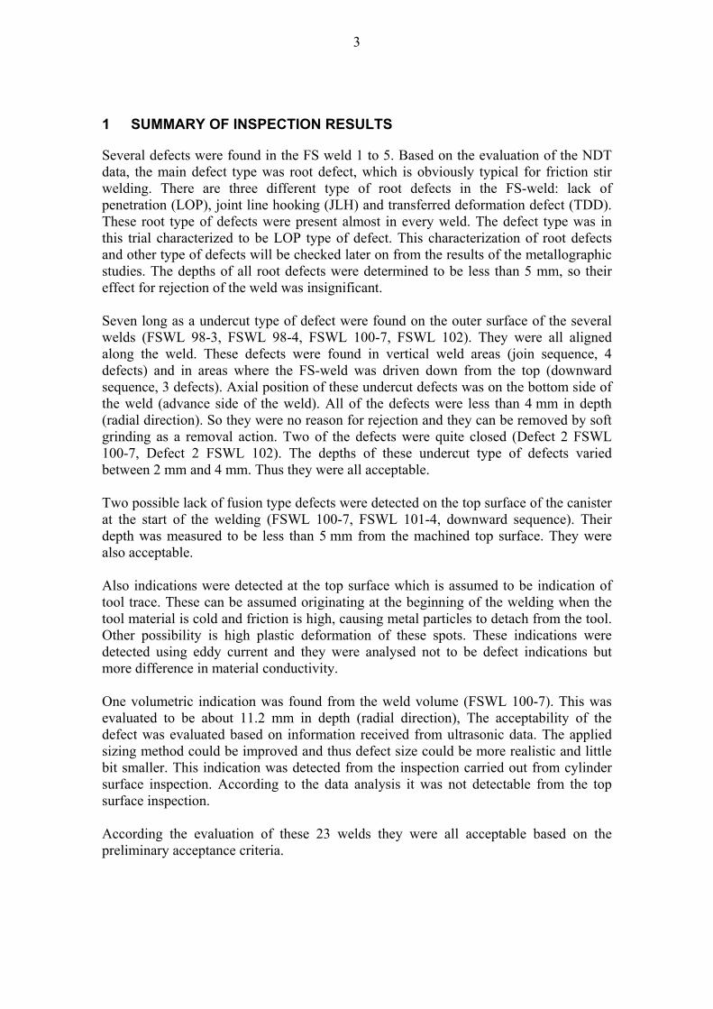
Several defects were found in the FS weld 1 to 5. Based on the evaluation of the NDT data, the main defect type was root defect, which is obviously typical for friction stir welding. There are three different type of root defects in the FS-weld: lack of penetration (LOP), joint line hooking (JLH) and transferred deformation defect (TDD). These root type of defects were present almost in every weld. The defect type was in this trial characterized to be LOP type of defect. This characterization of root defects and other type of defects will be checked later on from the results of the metallographic studies. The depths of all root defects were determined to be less than 5 mm, so their effect for rejection of the weld was insignificant. Seven long as a undercut type of defect were found on the outer surface of the several welds (FSWL 98-3, FSWL 98-4, FSWL 100-7, FSWL 102). They were all aligned along the weld. These defects were found in vertical weld areas (join sequence, 4 defects) and in areas where the FS-weld was driven down from the top (downward sequence, 3 defects). Axial position of these undercut defects was on the bottom side of the weld (advance side of the weld). All of the defects were less than 4 mm in depth (radial direction). So they were no reason for rejection and they can be removed by soft grinding as a removal action. Two of the defects were quite closed (Defect 2 FSWL 100-7, Defect 2 FSWL 102). The depths of these undercut type of defects varied between 2 mm and 4 mm. Thus they were all acceptable. Two possible lack of fusion type defects were detected on the top surface of the canister at the start of the welding (FSWL 100-7, FSWL 101-4, downward sequence). Their depth was measured to be less than 5 mm from the machined top surface. They were also acceptable. Also indications were detected at the top surface which is assumed to be indication of tool trace. These can be assumed originating at the beginning of the welding when the tool material is cold and friction is high, causing metal particles to detach from the tool. Other possibility is high plastic deformation of these spots. These indications were detected using eddy current and they were analysed not to be defect indications but more difference in material conductivity. One volumetric indication was found from the weld volume (FSWL 100-7). This was evaluated to be about 11.2 mm in depth (radial direction), The acceptability of the defect was evaluated based on information received from ultrasonic data. The applied sizing method could be improved and thus defect size could be more realistic and little bit smaller. This indication was detected from the inspection carried out from cylinder surface inspection. According to the data analysis it was not detectable from the top surface inspection. According the evaluation of these 23 welds they were all acceptable based on the preliminary acceptance criteria.

4
5
2 INTRODUCTION
In this report measurements and evaluation of five friction stir welding specimens is presented. Four basic NDT methods have been applied: visual testing (VT), eddy current testing (ET), ultrasonic testing (UT) and radiographic testing (RT). The applied NDT methods are presented in some details in the following chapter. The data acquisition and analysis has been discussed. The analysed data are presented in views related to that NDT method and data visualized in form of A- B-, C-, D- scans in ultrasonic testing and x-, y-, C-scans and Polar views in eddy current testing. Indications, which can be combined together according to proximity rules, are combined. The sizes of defects are determined according to the best knowledge, and visualized in different views. The acceptability of each weld has been reported according to today's preliminary acceptance criteria. Also it has to be pointed out, that these welds were done for parametric study, not for production of good welds. Only one full weld FS-weld (FSWL 103) was produced using optimal welding parameters in other welding series where it was several welds in one lid always the first weld was welded with optimal welding parameters (FSWL 98, 100 and 101) and from the weld FSWL 102 first 180 was welded with optimal welding parameters. Other welds have indications/defects which are related to not-optimal welding parameters. This can cause that those welds are rejected because of that.

6
7
3 APPLIED WELDING
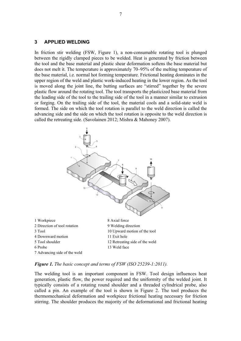
In friction stir welding (FSW, Figure 1), a non-consumable rotating tool is plunged between the rigidly clamped pieces to be welded. Heat is generated by friction between the tool and the base material and plastic shear deformation softens the base material but does not melt it. The temperature is approximately 70–95% of the melting temperature of the base material, i.e. normal hot forming temperature. Frictional heating dominates in the upper region of the weld and plastic work-induced heating in the lower region. As the tool is moved along the joint line, the butting surfaces are “stirred” together by the severe plastic flow around the rotating tool. The tool transports the plasticized base material from the leading side of the tool to the trailing side of the tool in a manner similar to extrusion or forging. On the trailing side of the tool, the material cools and a solid-state weld is formed. The side on which the tool rotation is parallel to the weld direction is called the advancing side and the side on which the tool rotation is opposite to the weld direction is called the retreating side. (Savolainen 2012; Mishra & Mahoney 2007).
1 Workpiece 8 Axial force 2 Direction of tool rotation 9 Welding direction 3 Tool 10 Upward motion of the tool 4 Downward motion 11 Exit hole 5 Tool shoulder 12 Retreating side of the weld 6 Probe 13 Weld face 7 Advancing side of the weld
Figure 1. The basic concept and terms of FSW (ISO 25239-1:2011).
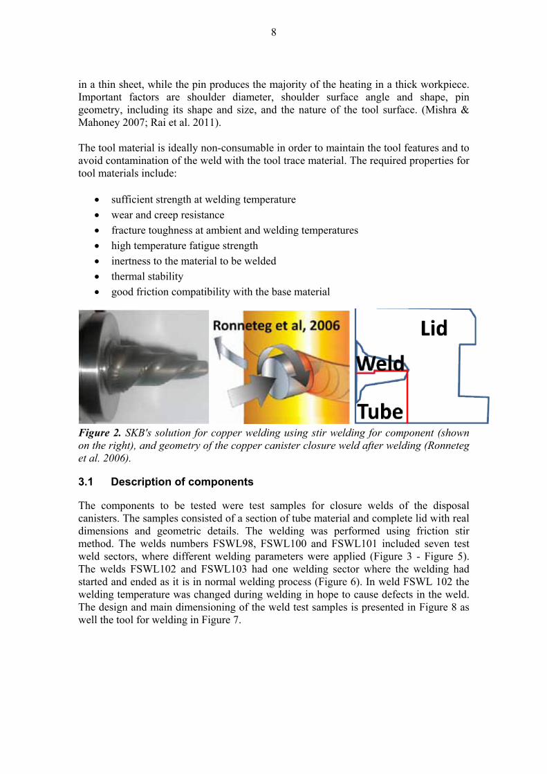
The welding tool is an important component in FSW. Tool design influences heat generation, plastic flow, the power required and the uniformity of the welded joint. It typically consists of a rotating round shoulder and a threaded cylindrical probe, also called a pin. An example of the tool is shown in Figure 2. The tool produces the thermomechanical deformation and workpiece frictional heating necessary for friction stirring. The shoulder produces the majority of the deformational and frictional heating
8
in a thin sheet, while the pin produces the majority of the heating in a thick workpiece. Important factors are shoulder diameter, shoulder surface angle and shape, pin geometry, including its shape and size, and the nature of the tool surface. (Mishra & Mahoney 2007; Rai et al. 2011). The tool material is ideally non-consumable in order to maintain the tool features and to avoid contamination of the weld with the tool trace material. The required properties for tool materials include:
sufficient strength at welding temperature
wear and creep resistance
fracture toughness at ambient and welding temperatures
high temperature fatigue strength
inertness to the material to be welded
thermal stability
good friction compatibility with the base material
Figure 2. SKB's solution for copper welding using stir welding for component (shown on the right), and geometry of the copper canister closure weld after welding (Ronneteg et al. 2006).
3.1 Description of components
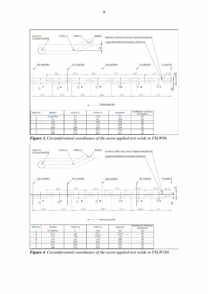
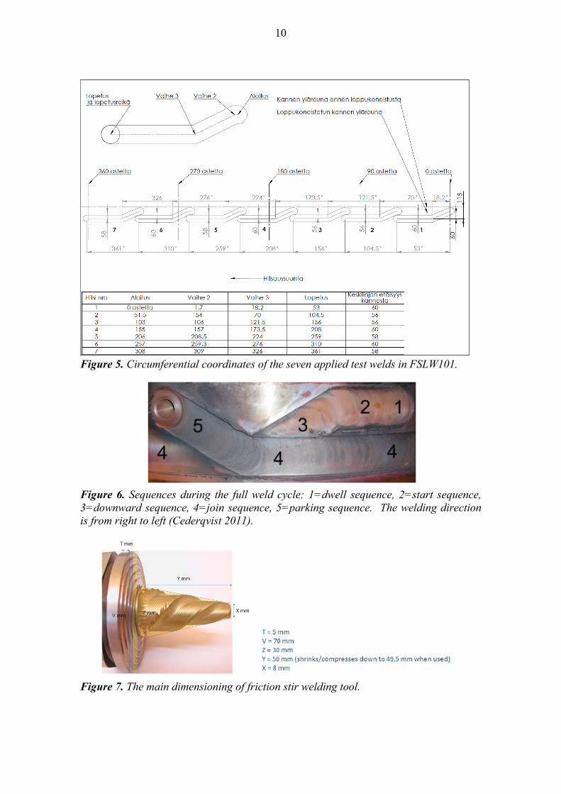
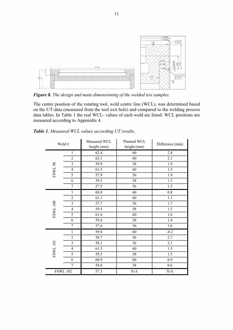
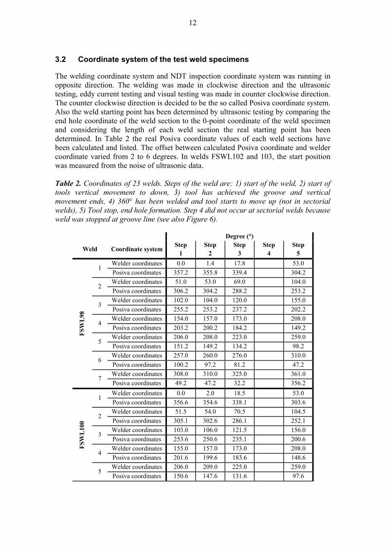
The components to be tested were test samples for closure welds of the disposal canisters. The samples consisted of a section of tube material and complete lid with real dimensions and geometric details. The welding was performed using friction stir method. The welds numbers FSWL98, FSWL100 and FSWL101 included seven test weld sectors, where different welding parameters were applied (Figure 3 - Figure 5). The welds FSWL102 and FSWL103 had one welding sector where the welding had started and ended as it is in normal welding process (Figure 6). In weld FSWL 102 the welding temperature was changed during welding in hope to cause defects in the weld. The design and main dimensioning of the weld test samples is presented in Figure 8 as well the tool for welding in Figure 7.
9
Figure 3. Circumferential coordinates of the seven applied test welds in FSLW98.
Figure 4. Circumferential coordinates of the seven applied test welds in FSLW100.
10
Figure 5. Circumferential coordinates of the seven applied test welds in FSLW101.
Figure 6. Sequences during the full weld cycle: 1=dwell sequence, 2=start sequence, 3=downward sequence, 4=join sequence, 5=parking sequence. The welding direction is from right to left (Cederqvist 2011).
Figure 7. The main dimensioning of friction stir welding tool.
11
Figure 8. The design and main dimensioning of the welded test samples.
The centre position of the rotating tool, weld centre line (WCL), was determined based on the UT-data (measured from the tool exit hole) and compared to the welding process data tables. In Table 1 the real WCL- values of each weld are listed. WCL positions are measured according to Appenidix 4. Table 1. Measured WCL values according UT results.
Weld # Measured WCL
height (mm) Planned WCL height (mm)
Difference (mm)
FS
WL
98
1 62.4 60 2.4
2 62.1 60 2.1
3 59.9 58 1.9
4 61.5 60 1.5
5 57.9 56 1.9
6 59.3 58 1.3
7 57.5 56 1.5
FS
WL
100
1 60.8 60 0.8
2 61.1 60 1.1
3 57.7 56 1.7
4 59.5 58 1.5
5 61.6 60 1.6
6 59.4 58 1.4
7 57.6 56 1.6
FS
WL
101
1 59.8 60 -0.2
2 58.7 56 2.7
3 58.1 56 2.1
4 61.5 60 1.5
5 59.5 58 1.5
6 60.9 60 0.9
7 58.6 58 0.6
FSWL 102 57.3 N/A N/A
12
3.2 Coordinate system of the test weld specimens
The welding coordinate system and NDT inspection coordinate system was running in opposite direction. The welding was made in clockwise direction and the ultrasonic testing, eddy current testing and visual testing was made in counter clockwise direction. The counter clockwise direction is decided to be the so called Posiva coordinate system. Also the weld starting point has been determined by ultrasonic testing by comparing the end hole coordinate of the weld section to the 0-point coordinate of the weld specimen and considering the length of each weld section the real starting point has been determined. In Table 2 the real Posiva coordinate values of each weld sections have been calculated and listed. The offset between calculated Posiva coordinate and welder coordinate varied from 2 to 6 degrees. In welds FSWL102 and 103, the start position was measured from the noise of ultrasonic data. Table 2. Coordinates of 23 welds. Steps of the weld are: 1) start of the weld, 2) start of tools vertical movement to down, 3) tool has achieved the groove and vertical movement ends, 4) 360° has been welded and tool starts to move up (not in sectorial welds), 5) Tool stop, end hole formation. Step 4 did not occur at sectorial welds because weld was stopped at groove line (see also Figure 6).
Degree (°)
Weld Coordinate systemStep
1 Step
2 Step
3 Step
4 Step
5
FS
WL
98
1 Welder coordinates 0.0 1.4 17.8 53.0
Posiva coordinates 357.2 355.8 339.4 304.2
2 Welder coordinates 51.0 53.0 69.0 104.0
Posiva coordinates 306.2 304.2 288.2 253.2
3 Welder coordinates 102.0 104.0 120.0 155.0
Posiva coordinates 255.2 253.2 237.2 202.2
4 Welder coordinates 154.0 157.0 173.0 208.0
Posiva coordinates 203.2 200.2 184.2 149.2
5 Welder coordinates 206.0 208.0 223.0 259.0
Posiva coordinates 151.2 149.2 134.2 98.2
6 Welder coordinates 257.0 260.0 276.0 310.0
Posiva coordinates 100.2 97.2 81.2 47.2
7 Welder coordinates 308.0 310.0 325.0 361.0
Posiva coordinates 49.2 47.2 32.2 356.2
FS
WL
100
1 Welder coordinates 0.0 2.0 18.5 53.0
Posiva coordinates 356.6 354.6 338.1 303.6
2 Welder coordinates 51.5 54.0 70.5 104.5
Posiva coordinates 305.1 302.6 286.1 252.1
3 Welder coordinates 103.0 106.0 121.5 156.0
Posiva coordinates 253.6 250.6 235.1 200.6
4 Welder coordinates 155.0 157.0 173.0 208.0
Posiva coordinates 201.6 199.6 183.6 148.6
5 Welder coordinates 206.0 209.0 225.0 259.0
Posiva coordinates 150.6 147.6 131.6 97.6

13
6 Welder coordinates 257.0 260.0 275.0 310.0
Posiva coordinates 99.6 96.6 81.6 46.6
7 Welder coordinates 308.0 310.0 325.0 361.0
Posiva coordinates 48.6 46.6 31.6 355.6
FS
WL
101
1 Welder coordinates 0.0 1.7 18.2 53.0
Posiva coordinates 2.9 1.2 344.7 309.9
2 Welder coordinates 51.5 54.0 70.0 104.5
Posiva coordinates 311.4 308.9 292.9 258.4
3 Welder coordinates 103.0 106.0 121.5 156.0
Posiva coordinates 259.9 256.9 241.4 206.9
4 Welder coordinates 155.0 157.0 173.5 208.0
Posiva coordinates 207.9 205.9 189.4 154.9
5 Welder coordinates 206.0 208.5 224.0 259.0
Posiva coordinates 156.9 154.4 138.9 103.9
6 Welder coordinates 257.0 259.3 276.0 310.0
Posiva coordinates 105.9 103.6 86.9 52.9
7 Welder coordinates 308.0 309.0 326.0 361.0
Posiva coordinates 54.9 53.9 36.9 1.9
FSWL102 Welder coordinates 0 0.0 2.0 18.0 382.0
Posiva coordinates 357 356.9 354.9 338.9 334.9
FSWL103 Welder coordinates 0 0.0 2.0 18.0 382.0
Posiva coordinates 354 354.3 352.3 336.3 332.3

14
15
4 DEFECT TYPES IN THE WELD
Following defect types can be found in FS-weld: Cavities, Joint line hooking, Lack of penetration, pores, flashes, entrapped oxide lines and tool traces.
4.1 Cavities
Cavities, also known as voids or wormholes, are volumetric, contain no material and are aligned to the welding direction and can be usually found on the advancing side. In some cases, voids are formed between the weld nugget and TMAZ. Cavities can occur from a lack of surface fill and can be observed by visual inspection; sometimes defects can be found by looking directly into the exit hole after the tool is retracted from the work piece. The higher the temperature achieved during welding, the more viscous the material and therefore the more easily it will flow and “fill in” these cavities. Conversely, the cooler the material the more it will stick to the pin as it rotates and leaves these cavities behind. (Lohwasser & Chen 2009; Savolainen 2012).
4.2 Entrapped oxide lines
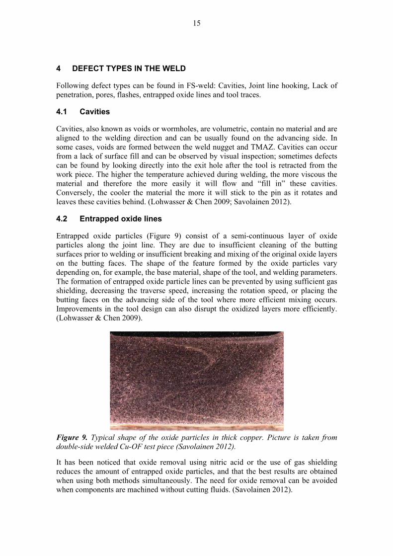
Entrapped oxide particles (Figure 9) consist of a semi-continuous layer of oxide particles along the joint line. They are due to insufficient cleaning of the butting surfaces prior to welding or insufficient breaking and mixing of the original oxide layers on the butting faces. The shape of the feature formed by the oxide particles vary depending on, for example, the base material, shape of the tool, and welding parameters. The formation of entrapped oxide particle lines can be prevented by using sufficient gas shielding, decreasing the traverse speed, increasing the rotation speed, or placing the butting faces on the advancing side of the tool where more efficient mixing occurs. Improvements in the tool design can also disrupt the oxidized layers more efficiently. (Lohwasser & Chen 2009).
Figure 9. Typical shape of the oxide particles in thick copper. Picture is taken from double-side welded Cu-OF test piece (Savolainen 2012).
It has been noticed that oxide removal using nitric acid or the use of gas shielding reduces the amount of entrapped oxide particles, and that the best results are obtained when using both methods simultaneously. The need for oxide removal can be avoided when components are machined without cutting fluids. (Savolainen 2012).
16
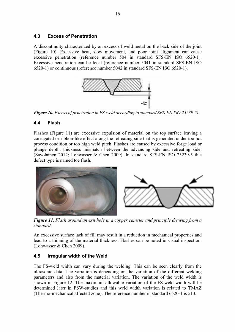
4.3 Excess of Penetration
A discontinuity characterized by an excess of weld metal on the back side of the joint (Figure 10). Excessive heat, slow movement, and poor joint alignment can cause excessive penetration (reference number 504 in standard SFS-EN ISO 6520-1). Excessive penetration can be local (reference number 5041 in standard SFS-EN ISO 6520-1) or continuous (reference number 5042 in standard SFS-EN ISO 6520-1).
Figure 10. Excess of penetration in FS-weld according to standard SFS-EN ISO 25239-5).
4.4 Flash
Flashes (Figure 11) are excessive expulsion of material on the top surface leaving a corrugated or ribbon-like effect along the retreating side that is generated under too hot process condition or too high weld pitch. Flashes are caused by excessive forge load or plunge depth, thickness mismatch between the advancing side and retreating side. (Savolainen 2012; Lohwasser & Chen 2009). In standard SFS-EN ISO 25239-5 this defect type is named toe flash.
Figure 11. Flash around an exit hole in a copper canister and principle drawing from a standard.
An excessive surface lack of fill may result in a reduction in mechanical properties and lead to a thinning of the material thickness. Flashes can be noted in visual inspection. (Lohwasser & Chen 2009).
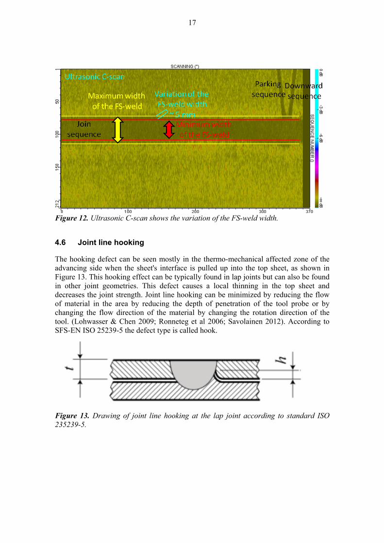
4.5 Irregular width of the Weld
The FS-weld width can vary during the welding. This can be seen clearly from the ultrasonic data. The variation is depending on the variation of the different welding parameters and also from the material variation. The variation of the weld width is shown in Figure 12. The maximum allowable variation of the FS-weld width will be determined later in FSW-studies and this weld width variation is related to TMAZ (Thermo-mechanical affected zone). The reference number in standard 6520-1 is 513.
17
Figure 12. Ultrasonic C-scan shows the variation of the FS-weld width.
4.6 Joint line hooking
The hooking defect can be seen mostly in the thermo-mechanical affected zone of the advancing side when the sheet's interface is pulled up into the top sheet, as shown in Figure 13. This hooking effect can be typically found in lap joints but can also be found in other joint geometries. This defect causes a local thinning in the top sheet and decreases the joint strength. Joint line hooking can be minimized by reducing the flow of material in the area by reducing the depth of penetration of the tool probe or by changing the flow direction of the material by changing the rotation direction of the tool. (Lohwasser & Chen 2009; Ronneteg et al 2006; Savolainen 2012). According to SFS-EN ISO 25239-5 the defect type is called hook.
Figure 13. Drawing of joint line hooking at the lap joint according to standard ISO 235239-5.
18
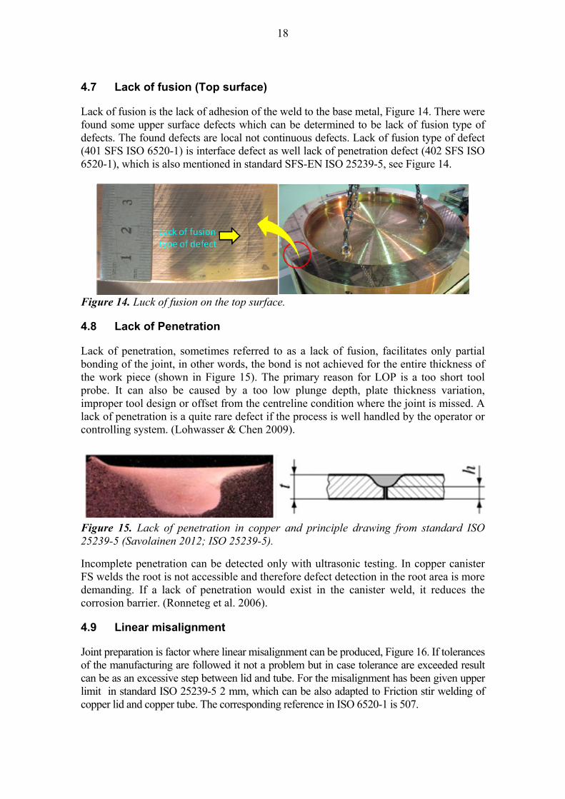
4.7 Lack of fusion (Top surface)
Lack of fusion is the lack of adhesion of the weld to the base metal, Figure 14. There were found some upper surface defects which can be determined to be lack of fusion type of defects. The found defects are local not continuous defects. Lack of fusion type of defect (401 SFS ISO 6520-1) is interface defect as well lack of penetration defect (402 SFS ISO 6520-1), which is also mentioned in standard SFS-EN ISO 25239-5, see Figure 14.
Figure 14. Luck of fusion on the top surface.
4.8 Lack of Penetration
Lack of penetration, sometimes referred to as a lack of fusion, facilitates only partial bonding of the joint, in other words, the bond is not achieved for the entire thickness of the work piece (shown in Figure 15). The primary reason for LOP is a too short tool probe. It can also be caused by a too low plunge depth, plate thickness variation, improper tool design or offset from the centreline condition where the joint is missed. A lack of penetration is a quite rare defect if the process is well handled by the operator or controlling system. (Lohwasser & Chen 2009).
Figure 15. Lack of penetration in copper and principle drawing from standard ISO 25239-5 (Savolainen 2012; ISO 25239-5).
Incomplete penetration can be detected only with ultrasonic testing. In copper canister FS welds the root is not accessible and therefore defect detection in the root area is more demanding. If a lack of penetration would exist in the canister weld, it reduces the corrosion barrier. (Ronneteg et al. 2006).
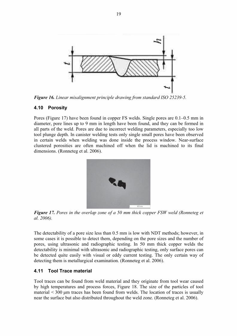
4.9 Linear misalignment
Joint preparation is factor where linear misalignment can be produced, Figure 16. If tolerances of the manufacturing are followed it not a problem but in case tolerance are exceeded result can be as an excessive step between lid and tube. For the misalignment has been given upper limit in standard ISO 25239-5 2 mm, which can be also adapted to Friction stir welding of copper lid and copper tube. The corresponding reference in ISO 6520-1 is 507.
19
Figure 16. Linear misalignment principle drawing from standard ISO 25239-5.
4.10 Porosity
Pores (Figure 17) have been found in copper FS welds. Single pores are 0.1–0.5 mm in diameter, pore lines up to 9 mm in length have been found, and they can be formed in all parts of the weld. Pores are due to incorrect welding parameters, especially too low tool plunge depth. In canister welding tests only single small pores have been observed in certain welds when welding was done inside the process window. Near-surface clustered porosities are often machined off when the lid is machined to its final dimensions. (Ronneteg et al. 2006).
Figure 17. Pores in the overlap zone of a 50 mm thick copper FSW weld (Ronneteg et al. 2006).
The detectability of a pore size less than 0.5 mm is low with NDT methods; however, in some cases it is possible to detect them, depending on the pore sizes and the number of pores, using ultrasonic and radiographic testing. In 50 mm thick copper welds the detectability is minimal with ultrasonic and radiographic testing, only surface pores can be detected quite easily with visual or eddy current testing. The only certain way of detecting them is metallurgical examination. (Ronneteg et al. 2006).
4.11 Tool Trace material
Tool traces can be found from weld material and they originate from tool wear caused by high temperatures and process forces, Figure 18. The size of the particles of tool material < 300 μm traces has been found from welds. The location of traces is usually near the surface but also distributed throughout the weld zone. (Ronneteg et al. 2006).
20
Figure 18. Traces of foreign material (W) near-surface in unmachined lid weld 20 (Ronneteg et al. 2006). The surface treatment of tools has reduced trace levels. In metallurgical examination it has been observed that at the moment the composition of impurities in the weld is very low. Traces can be detected mainly by chemical analysis. (Ronneteg et al. 2006).
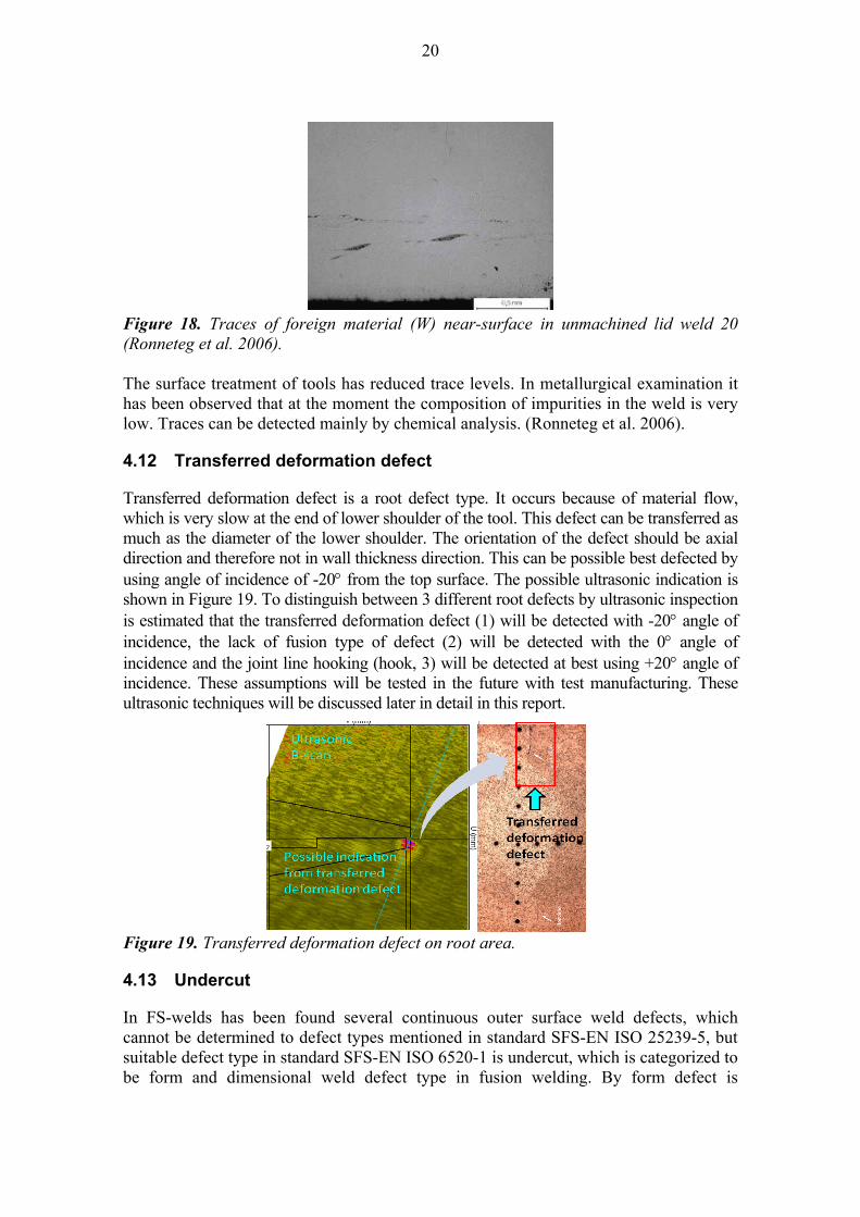
4.12 Transferred deformation defect
Transferred deformation defect is a root defect type. It occurs because of material flow, which is very slow at the end of lower shoulder of the tool. This defect can be transferred as much as the diameter of the lower shoulder. The orientation of the defect should be axial direction and therefore not in wall thickness direction. This can be possible best defected by using angle of incidence of -20 from the top surface. The possible ultrasonic indication is shown in Figure 19. To distinguish between 3 different root defects by ultrasonic inspection is estimated that the transferred deformation defect (1) will be detected with -20 angle of incidence, the lack of fusion type of defect (2) will be detected with the 0 angle of incidence and the joint line hooking (hook, 3) will be detected at best using +20 angle of incidence. These assumptions will be tested in the future with test manufacturing. These ultrasonic techniques will be discussed later in detail in this report.
Figure 19. Transferred deformation defect on root area.
4.13 Undercut
In FS-welds has been found several continuous outer surface weld defects, which cannot be determined to defect types mentioned in standard SFS-EN ISO 25239-5, but suitable defect type in standard SFS-EN ISO 6520-1 is undercut, which is categorized to be form and dimensional weld defect type in fusion welding. By form defect is
21
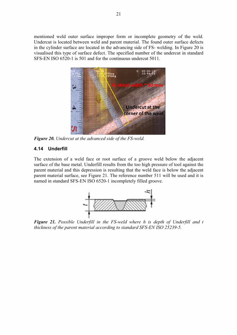
mentioned weld outer surface improper form or incomplete geometry of the weld. Undercut is located between weld and parent material. The found outer surface defects in the cylinder surface are located in the advancing side of FS- welding. In Figure 20 is visualised this type of surface defect. The specified number of the undercut in standard SFS-EN ISO 6520-1 is 501 and for the continuous undercut 5011.
Figure 20. Undercut at the advanced side of the FS-weld.
4.14 Underfill
The extension of a weld face or root surface of a groove weld below the adjacent surface of the base metal. Underfill results from the too high pressure of tool against the parent material and this depression is resulting that the weld face is below the adjacent parent material surface, see Figure 21. The reference number 511 will be used and it is named in standard SFS-EN ISO 6520-1 incompletely filled groove.
Figure 21. Possible Underfill in the FS-weld where h is depth of Underfill and t thickness of the parent material according to standard SFS-EN ISO 25239-5.

22

23
5 ACCEPTANCE AND REJECTION CRITERIA
Primary acceptance criteria for welds in this welding test are presented in Table 3. Table 3. Preliminary acceptance criteria for the canister sealing welds in the lid test series. The acceptance criteria for different defect types are modified according to remaining wall thickness criterion and completed with thick copper weld defects types (FS-weld).
Symbols in Table 3 are as follows: l length of defect, w width of defect, h height of defect.
Defect No.
Type of defect /surface defect removal action Maximum allowable size
100 Cracks l < 10 mm, h < 3 mm
2011, 200 Gas pore, porosity l < 25 mm, h < 6 mm, w ≤ 8 mm
2013 Clustered porosity l < 25 mm, h < 6 mm, w ≤ 8 mm
2014 Linear porosity l < 25 mm, h < 6 mm, w ≤ 8 mm
2015 Elongated cavity l < 25 mm, h < 6 mm, w ≤ 8 mm
similar location in the weld as 5011, 5012
External undercut, defect on the side of the weld originating machining and welding, possible defect removal by smooth grinding
l < 20 mm, h < 5 mm Continuous undercut type of defect l: continuous, h< 4 mm, defect removal action possible until 5 mm surface depth
402 Incomplete or excessive penetration ISO 25239-5) l continuous, h < 8 mm, Intact 42 mm
Joint line hooking ( Hook - ISO 25239-5) l continuous, h < 8 mm, Intact 42 mm
similar to 401
Lack of joint l < 50 mm, h < 10 mm Surface breaking l, w < 50 mm, h < 5 mm (Axial, Top surface)
Transferred deformation defect l continuous, h, w < 8 mm
2016 Wormhole / Crater l w≤ 20 mm , h ≤ 10 mm
300 Solid inclusions l ≤ 10 mm, w ≤ 3 mm, h < 10 mm
511 Incompletely filled groove
l < 10 mm, w < 8 mm, h < 5 mm, Continuous incompletely filled groove, l: continuous, h< 4 mm, defect removal action possible until 5 mm surface depth
513 Irregular weld width variation of the weld width < 12 mm
507 Linear misalignment linear misalignment < 2 mm
Scratches Permitted locally
Indentation
1 mm depth, large diameter indentation (d > 10 mm), small and sharp indentations (scratch-like) are allowed
Removal action of a surface defect
Geometric deviation caused by smooth grinding (allowable 10% of nominal wall thickness)
l continuous, h ≤5 mm; remaining wall thickness (intact material) should be at least 35 mm after grinding in the grinded area

24
The determination of the height of the defect depends on the location of the defect- If defect is on the top or near the top surface the height of the defect is axial direction and length in circumferential direction the and width is in radial direction. When the minimum intact is in the radial direction the height of the defect is of course in this direction and length in the circumferential direction and width of the defect in the axial direction. Any two adjacent defects separated by a distance smaller than the major dimension of the smaller defects shall be considered as a single defect. The criterion covering the intact wall thickness requirement of 35 mm in 100 % and 40 mm in 99 % of the canisters is the master requirement for acceptance, especially for combining defects. The indications detected in inspections are first evaluated in the screening phase according to acceptance criteria (Table 3) keeping in mind the master requirement of the intact wall thickness. This acceptance and rejection process is shown in Figure 22. The evaluation of the indications shall be carried out by qualified personnel (detection and sizing qualification). If acceptance criteria presented in Table 3 are exceeded but total defect length is less than 6 % of the total weld length then the weld is acceptable taking into account that the weld thickness requirement of 35 mm in 100 % length of the weld is met.
Figure 22. Acceptance and rejection process of the final disposal canister sealing weld based on the evaluation of the NDT measurements.
25
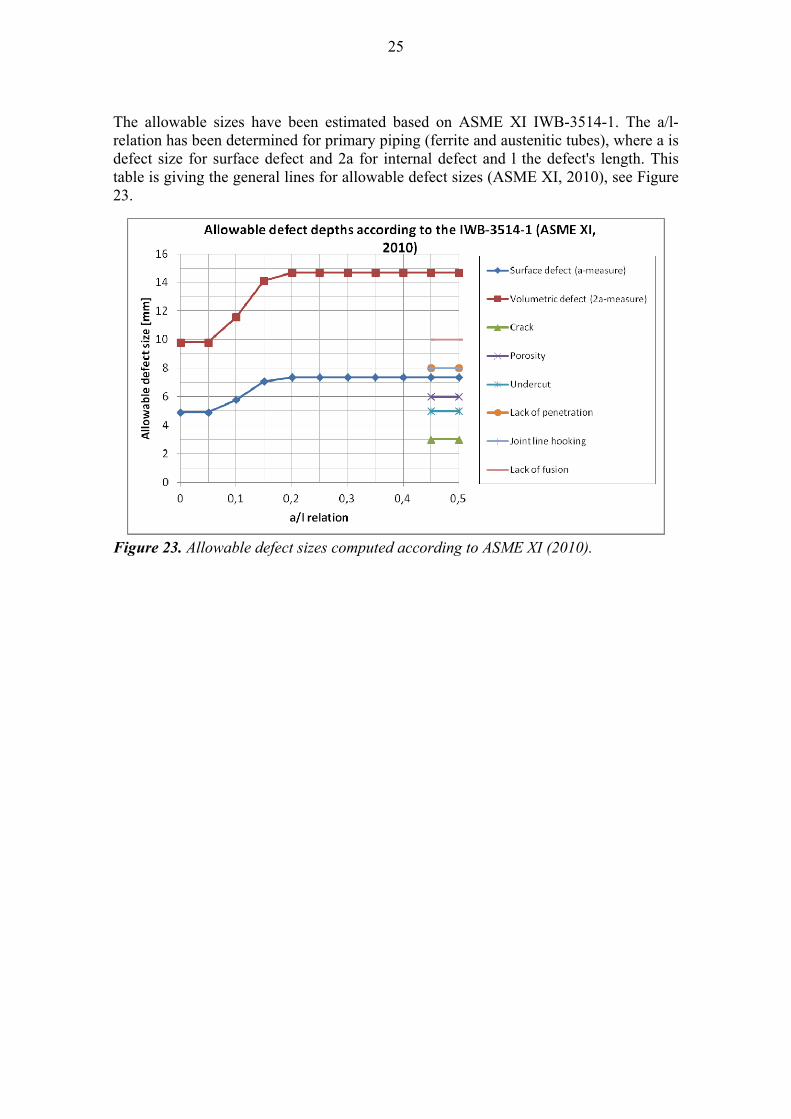
The allowable sizes have been estimated based on ASME XI IWB-3514-1. The a/l-relation has been determined for primary piping (ferrite and austenitic tubes), where a is defect size for surface defect and 2a for internal defect and l the defect's length. This table is giving the general lines for allowable defect sizes (ASME XI, 2010), see Figure 23.
Figure 23. Allowable defect sizes computed according to ASME XI (2010).

26
27
6 APPLIED NDT METHODS
6.1 Defect detection techniques
The applied NDT test methods were phased array ultrasonic testing, eddy current testing, radiographic testing and visual testing.
6.1.1 Ultrasonic testing
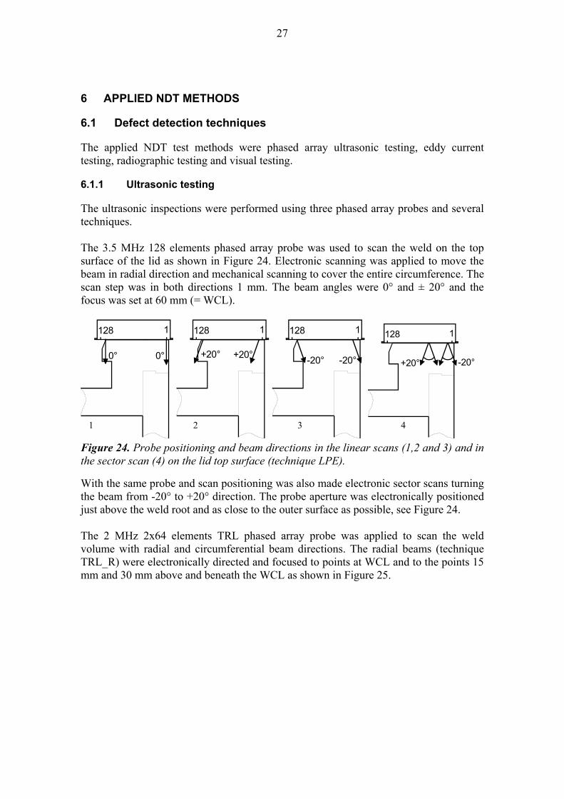
The ultrasonic inspections were performed using three phased array probes and several techniques. The 3.5 MHz 128 elements phased array probe was used to scan the weld on the top surface of the lid as shown in Figure 24. Electronic scanning was applied to move the beam in radial direction and mechanical scanning to cover the entire circumference. The scan step was in both directions 1 mm. The beam angles were 0° and ± 20° and the focus was set at 60 mm (= WCL).
1128
0° 0°
1128
+20° +20°
1128
-20°-20°
1128
-20°+20°
Figure 24. Probe positioning and beam directions in the linear scans (1,2 and 3) and in the sector scan (4) on the lid top surface (technique LPE).
With the same probe and scan positioning was also made electronic sector scans turning the beam from -20° to +20° direction. The probe aperture was electronically positioned just above the weld root and as close to the outer surface as possible, see Figure 24. The 2 MHz 2x64 elements TRL phased array probe was applied to scan the weld volume with radial and circumferential beam directions. The radial beams (technique TRL_R) were electronically directed and focused to points at WCL and to the points 15 mm and 30 mm above and beneath the WCL as shown in Figure 25.
1 2 3 4
28
60
15
WCL
PROBE
30 focus points in each line
15
15
15
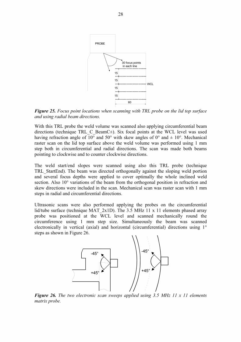
Figure 25. Focus point locations when scanning with TRL probe on the lid top surface and using radial beam directions.
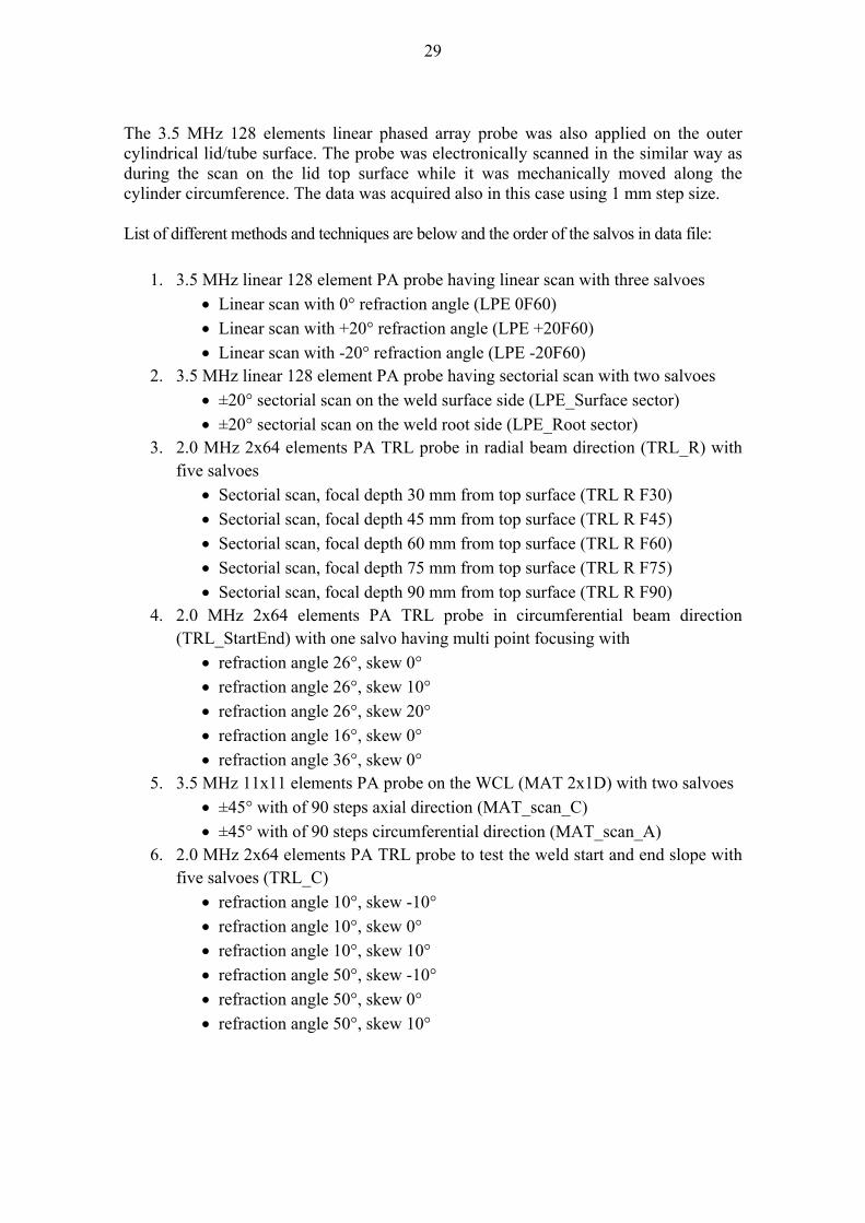
With this TRL probe the weld volume was scanned also applying circumferential beam directions (technique TRL_C_BeamC±). Six focal points at the WCL level was used having refraction angle of 10° and 50° with skew angles of 0° and ± 10°. Mechanical raster scan on the lid top surface above the weld volume was performed using 1 mm step both in circumferential and radial directions. The scan was made both beams pointing to clockwise and to counter clockwise directions. The weld start/end slopes were scanned using also this TRL probe (technique TRL_StartEnd). The beam was directed orthogonally against the sloping weld portion and several focus depths were applied to cover optimally the whole inclined weld section. Also 10° variations of the beam from the orthogonal position in refraction and skew directions were included in the scan. Mechanical scan was raster scan with 1 mm steps in radial and circumferential directions. Ultrasonic scans were also performed applying the probes on the circumferential lid/tube surface (technique MAT_2x1D). The 3.5 MHz 11 x 11 elements phased array probe was positioned at the WCL level and scanned mechanically round the circumference using 1 mm step size. Simultaneously the beam was scanned electronically in vertical (axial) and horizontal (circumferential) directions using 1° steps as shown in Figure 26.
-45°
+45°
-45°
+45°
Figure 26. The two electronic scan sweeps applied using 3.5 MHz 11 x 11 elements matrix probe.
29
The 3.5 MHz 128 elements linear phased array probe was also applied on the outer cylindrical lid/tube surface. The probe was electronically scanned in the similar way as during the scan on the lid top surface while it was mechanically moved along the cylinder circumference. The data was acquired also in this case using 1 mm step size. List of different methods and techniques are below and the order of the salvos in data file:
1. 3.5 MHz linear 128 element PA probe having linear scan with three salvoes
Linear scan with 0° refraction angle (LPE 0F60)
Linear scan with +20° refraction angle (LPE +20F60)
Linear scan with -20° refraction angle (LPE -20F60) 2. 3.5 MHz linear 128 element PA probe having sectorial scan with two salvoes
±20° sectorial scan on the weld surface side (LPE_Surface sector)
±20° sectorial scan on the weld root side (LPE_Root sector) 3. 2.0 MHz 2x64 elements PA TRL probe in radial beam direction (TRL_R) with
five salvoes
Sectorial scan, focal depth 30 mm from top surface (TRL R F30)
Sectorial scan, focal depth 45 mm from top surface (TRL R F45)
Sectorial scan, focal depth 60 mm from top surface (TRL R F60)
Sectorial scan, focal depth 75 mm from top surface (TRL R F75)
Sectorial scan, focal depth 90 mm from top surface (TRL R F90) 4. 2.0 MHz 2x64 elements PA TRL probe in circumferential beam direction
(TRL_StartEnd) with one salvo having multi point focusing with
refraction angle 26°, skew 0°
refraction angle 26°, skew 10°
refraction angle 26°, skew 20°
refraction angle 16°, skew 0°
refraction angle 36°, skew 0° 5. 3.5 MHz 11x11 elements PA probe on the WCL (MAT 2x1D) with two salvoes
±45° with of 90 steps axial direction (MAT_scan_C)
±45° with of 90 steps circumferential direction (MAT_scan_A) 6. 2.0 MHz 2x64 elements PA TRL probe to test the weld start and end slope with
five salvoes (TRL_C)
refraction angle 10°, skew -10°
refraction angle 10°, skew 0°
refraction angle 10°, skew 10°
refraction angle 50°, skew -10°
refraction angle 50°, skew 0°
refraction angle 50°, skew 10°
30
6.1.2 Eddy Current techniques
Three different eddy current techniques were applied to each weld. 1. High Frequency (HF) technique with 30kHz absolute pancake coils 2. Low frequency (LF0°) technique with 203 Hz having one transmitter coil and
two receiver coils in circumferential direction 3. Low frequency (LF90°) technique with 203 Hz having one transmitter coil and
two receiver coils in axial direction. The tested surface areas are marked in Figure 27.
6.1.3 Visual inspection
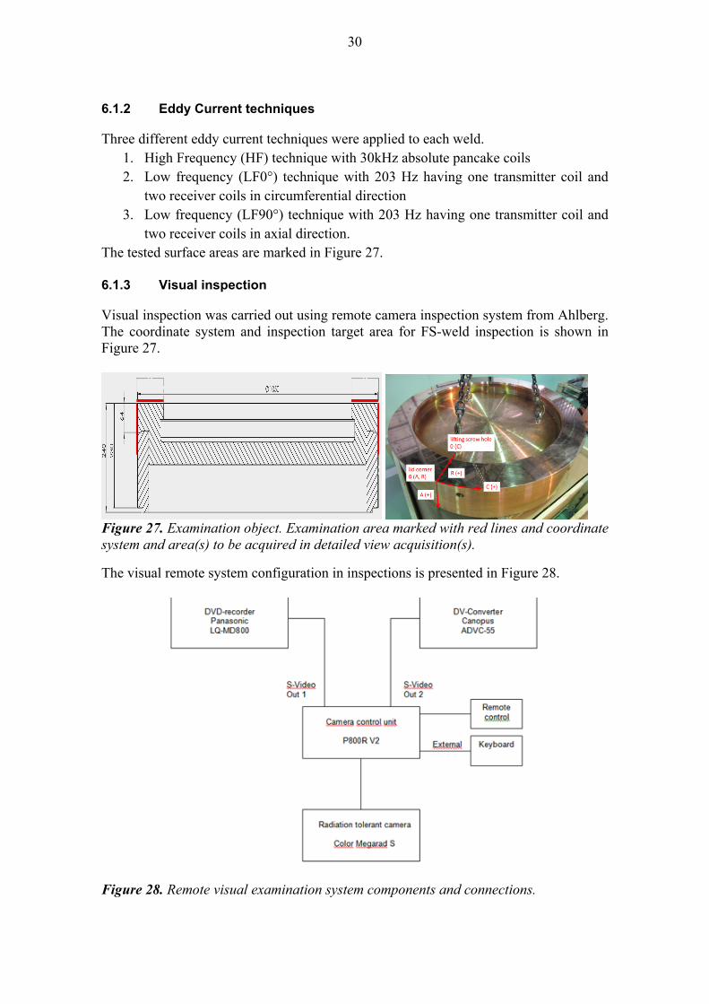
Visual inspection was carried out using remote camera inspection system from Ahlberg. The coordinate system and inspection target area for FS-weld inspection is shown in Figure 27.
Figure 27. Examination object. Examination area marked with red lines and coordinate system and area(s) to be acquired in detailed view acquisition(s).
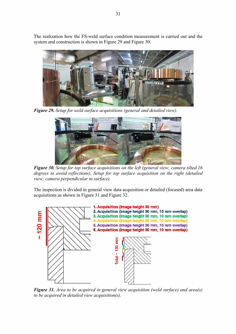
The visual remote system configuration in inspections is presented in Figure 28.
Figure 28. Remote visual examination system components and connections.
31
The realization how the FS-weld surface condition measurement is carried out and the system and construction is shown in Figure 29 and Figure 30.
Figure 29. Setup for weld surface acquisitions (general and detailed view).
Figure 30. Setup for top surface acquisitions on the left (general view; camera tilted 16 degrees to avoid reflections), Setup for top surface acquisition on the right (detailed view; camera perpendicular to surface). The inspection is divided in general view data acquisition or detailed (focused) area data acquisitions as shown in Figure 31 and Figure 32.
Figure 31. Area to be acquired in general view acquisition (weld surface) and area(s) to be acquired in detailed view acquisition(s).
32
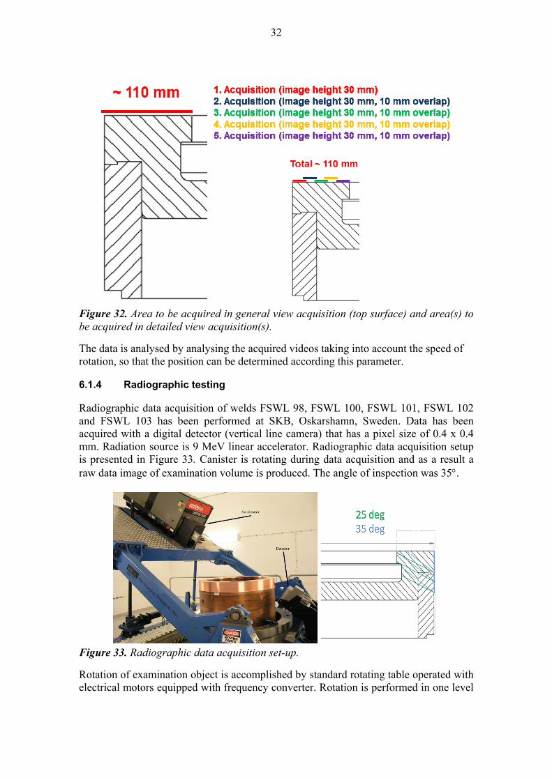
Figure 32. Area to be acquired in general view acquisition (top surface) and area(s) to be acquired in detailed view acquisition(s).
The data is analysed by analysing the acquired videos taking into account the speed of rotation, so that the position can be determined according this parameter.
6.1.4 Radiographic testing
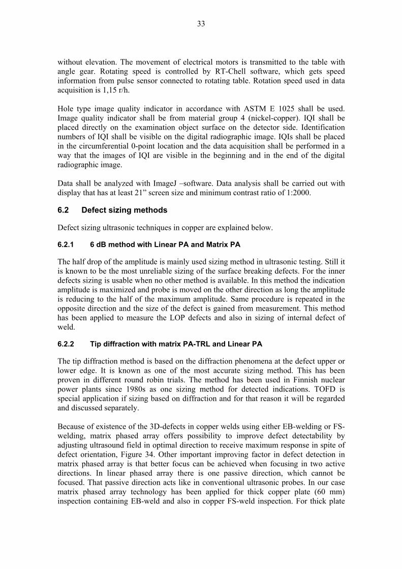
Radiographic data acquisition of welds FSWL 98, FSWL 100, FSWL 101, FSWL 102 and FSWL 103 has been performed at SKB, Oskarshamn, Sweden. Data has been acquired with a digital detector (vertical line camera) that has a pixel size of 0.4 x 0.4 mm. Radiation source is 9 MeV linear accelerator. Radiographic data acquisition setup is presented in Figure 33. Canister is rotating during data acquisition and as a result a raw data image of examination volume is produced. The angle of inspection was 35.
Figure 33. Radiographic data acquisition set-up.
Rotation of examination object is accomplished by standard rotating table operated with electrical motors equipped with frequency converter. Rotation is performed in one level
33
without elevation. The movement of electrical motors is transmitted to the table with angle gear. Rotating speed is controlled by RT-Chell software, which gets speed information from pulse sensor connected to rotating table. Rotation speed used in data acquisition is 1,15 r/h. Hole type image quality indicator in accordance with ASTM E 1025 shall be used. Image quality indicator shall be from material group 4 (nickel-copper). IQI shall be placed directly on the examination object surface on the detector side. Identification numbers of IQI shall be visible on the digital radiographic image. IQIs shall be placed in the circumferential 0-point location and the data acquisition shall be performed in a way that the images of IQI are visible in the beginning and in the end of the digital radiographic image. Data shall be analyzed with ImageJ –software. Data analysis shall be carried out with display that has at least 21” screen size and minimum contrast ratio of 1:2000.
6.2 Defect sizing methods
Defect sizing ultrasonic techniques in copper are explained below.
6.2.1 6 dB method with Linear PA and Matrix PA
The half drop of the amplitude is mainly used sizing method in ultrasonic testing. Still it is known to be the most unreliable sizing of the surface breaking defects. For the inner defects sizing is usable when no other method is available. In this method the indication amplitude is maximized and probe is moved on the other direction as long the amplitude is reducing to the half of the maximum amplitude. Same procedure is repeated in the opposite direction and the size of the defect is gained from measurement. This method has been applied to measure the LOP defects and also in sizing of internal defect of weld.
6.2.2 Tip diffraction with matrix PA-TRL and Linear PA
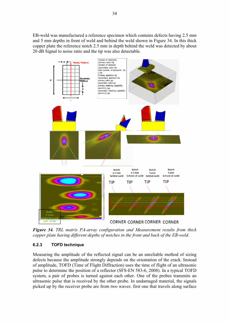
The tip diffraction method is based on the diffraction phenomena at the defect upper or lower edge. It is known as one of the most accurate sizing method. This has been proven in different round robin trials. The method has been used in Finnish nuclear power plants since 1980s as one sizing method for detected indications. TOFD is special application if sizing based on diffraction and for that reason it will be regarded and discussed separately. Because of existence of the 3D-defects in copper welds using either EB-welding or FS-welding, matrix phased array offers possibility to improve defect detectability by adjusting ultrasound field in optimal direction to receive maximum response in spite of defect orientation, Figure 34. Other important improving factor in defect detection in matrix phased array is that better focus can be achieved when focusing in two active directions. In linear phased array there is one passive direction, which cannot be focused. That passive direction acts like in conventional ultrasonic probes. In our case matrix phased array technology has been applied for thick copper plate (60 mm) inspection containing EB-weld and also in copper FS-weld inspection. For thick plate
34
EB-weld was manufactured a reference specimen which contains defects having 2.5 mm and 5 mm depths in front of weld and behind the weld shown in Figure 34. In this thick copper plate the reference notch 2.5 mm in depth behind the weld was detected by about 20 dB Signal to noise ratio and the tip was also detectable.
Figure 34. TRL matrix PA-array configuration and Measurement results from thick copper plate having different depths of notches in the front and back of the EB-weld.
6.2.3 TOFD technique
Measuring the amplitude of the reflected signal can be an unreliable method of sizing defects because the amplitude strongly depends on the orientation of the crack. Instead of amplitude, TOFD (Time of Flight Diffraction) uses the time of flight of an ultrasonic pulse to determine the position of a reflector (SFS-EN 583-6, 2008). In a typical TOFD system, a pair of probes is turned against each other. One of the probes transmits an ultrasonic pulse that is received by the other probe. In undamaged material, the signals picked up by the receiver probe are from two waves: first one that travels along surface
35
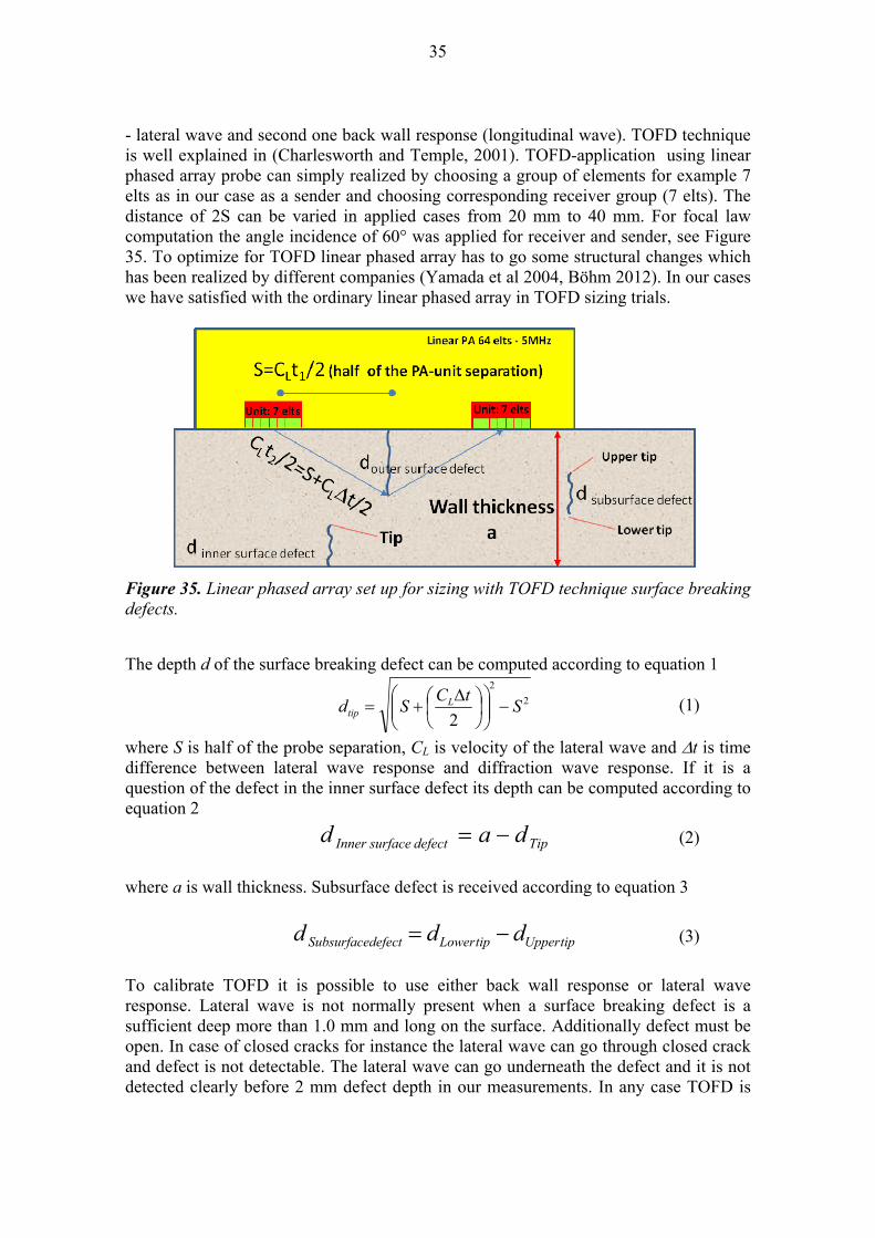
- lateral wave and second one back wall response (longitudinal wave). TOFD technique is well explained in (Charlesworth and Temple, 2001). TOFD-application using linear phased array probe can simply realized by choosing a group of elements for example 7 elts as in our case as a sender and choosing corresponding receiver group (7 elts). The distance of 2S can be varied in applied cases from 20 mm to 40 mm. For focal law computation the angle incidence of 60° was applied for receiver and sender, see Figure 35. To optimize for TOFD linear phased array has to go some structural changes which has been realized by different companies (Yamada et al 2004, Böhm 2012). In our cases we have satisfied with the ordinary linear phased array in TOFD sizing trials.
Figure 35. Linear phased array set up for sizing with TOFD technique surface breaking defects.
The depth d of the surface breaking defect can be computed according to equation 1
2
2
2S
tCSd L
tip
(1)
where S is half of the probe separation, CL is velocity of the lateral wave and t is time difference between lateral wave response and diffraction wave response. If it is a question of the defect in the inner surface defect its depth can be computed according to equation 2
TipdefectsurfaceInner dad (2)
where a is wall thickness. Subsurface defect is received according to equation 3
tipUppertipLowerdefectSubsurface ddd (3)
To calibrate TOFD it is possible to use either back wall response or lateral wave response. Lateral wave is not normally present when a surface breaking defect is a sufficient deep more than 1.0 mm and long on the surface. Additionally defect must be open. In case of closed cracks for instance the lateral wave can go through closed crack and defect is not detectable. The lateral wave can go underneath the defect and it is not detected clearly before 2 mm defect depth in our measurements. In any case TOFD is
36
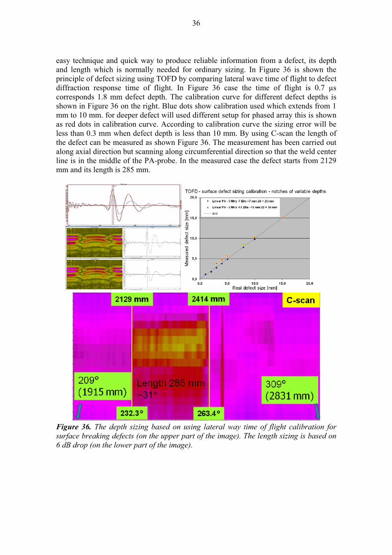
easy technique and quick way to produce reliable information from a defect, its depth and length which is normally needed for ordinary sizing. In Figure 36 is shown the principle of defect sizing using TOFD by comparing lateral wave time of flight to defect diffraction response time of flight. In Figure 36 case the time of flight is 0.7 µs corresponds 1.8 mm defect depth. The calibration curve for different defect depths is shown in Figure 36 on the right. Blue dots show calibration used which extends from 1 mm to 10 mm. for deeper defect will used different setup for phased array this is shown as red dots in calibration curve. According to calibration curve the sizing error will be less than 0.3 mm when defect depth is less than 10 mm. By using C-scan the length of the defect can be measured as shown Figure 36. The measurement has been carried out along axial direction but scanning along circumferential direction so that the weld center line is in the middle of the PA-probe. In the measured case the defect starts from 2129 mm and its length is 285 mm.
Figure 36. The depth sizing based on using lateral way time of flight calibration for surface breaking defects (on the upper part of the image). The length sizing is based on 6 dB drop (on the lower part of the image).
37
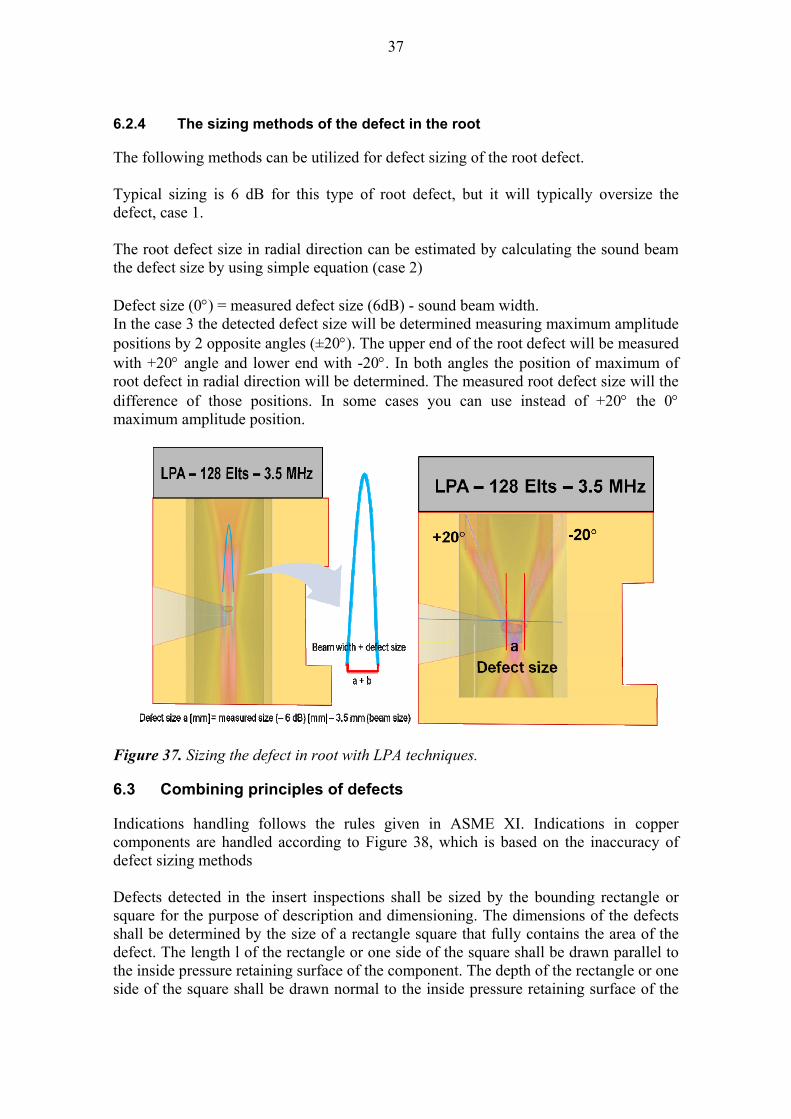
6.2.4 The sizing methods of the defect in the root
The following methods can be utilized for defect sizing of the root defect. Typical sizing is 6 dB for this type of root defect, but it will typically oversize the defect, case 1. The root defect size in radial direction can be estimated by calculating the sound beam the defect size by using simple equation (case 2) Defect size (0) = measured defect size (6dB) - sound beam width. In the case 3 the detected defect size will be determined measuring maximum amplitude positions by 2 opposite angles (±20). The upper end of the root defect will be measured with +20 angle and lower end with -20. In both angles the position of maximum of root defect in radial direction will be determined. The measured root defect size will the difference of those positions. In some cases you can use instead of +20 the 0 maximum amplitude position.
Figure 37. Sizing the defect in root with LPA techniques.
6.3 Combining principles of defects
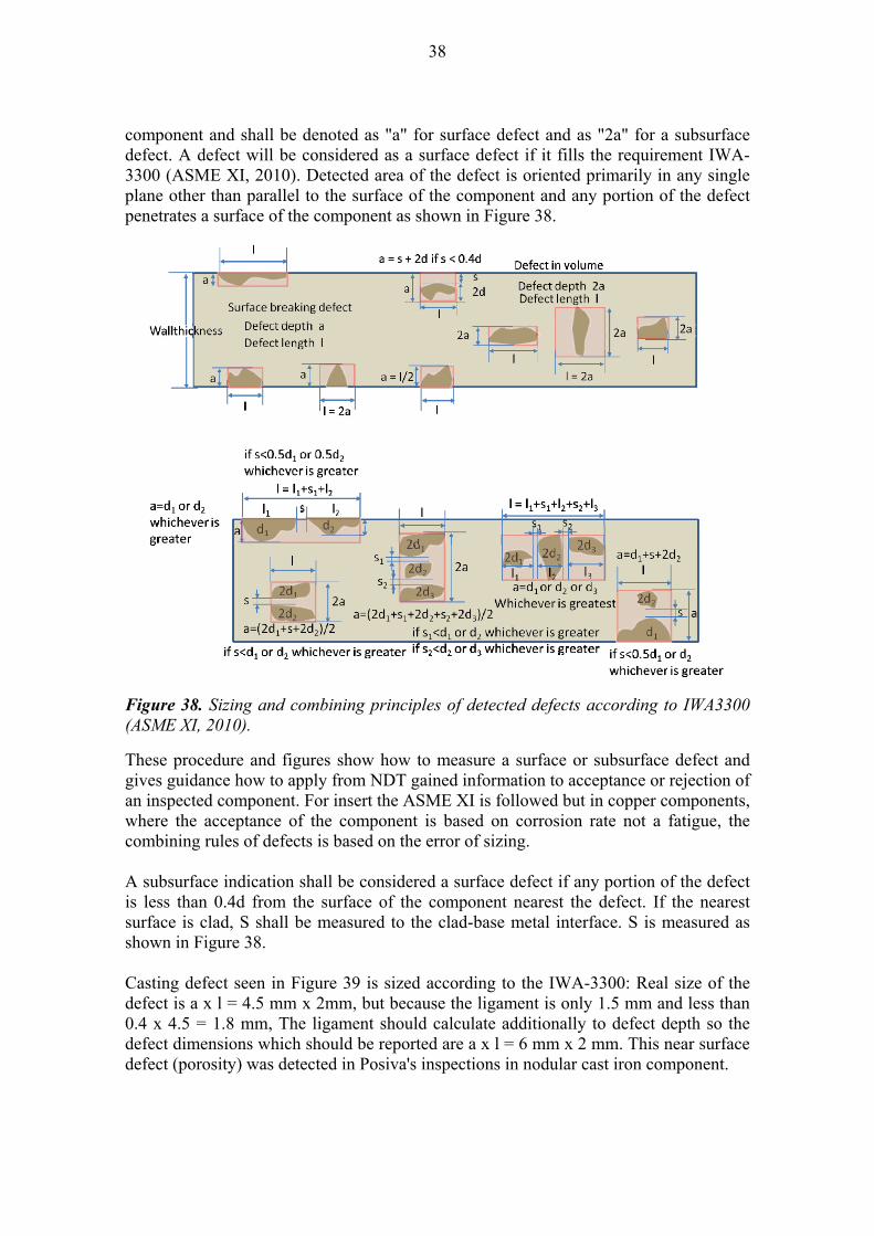
Indications handling follows the rules given in ASME XI. Indications in copper components are handled according to Figure 38, which is based on the inaccuracy of defect sizing methods Defects detected in the insert inspections shall be sized by the bounding rectangle or square for the purpose of description and dimensioning. The dimensions of the defects shall be determined by the size of a rectangle square that fully contains the area of the defect. The length l of the rectangle or one side of the square shall be drawn parallel to the inside pressure retaining surface of the component. The depth of the rectangle or one side of the square shall be drawn normal to the inside pressure retaining surface of the
38
component and shall be denoted as "a" for surface defect and as "2a" for a subsurface defect. A defect will be considered as a surface defect if it fills the requirement IWA-3300 (ASME XI, 2010). Detected area of the defect is oriented primarily in any single plane other than parallel to the surface of the component and any portion of the defect penetrates a surface of the component as shown in Figure 38.
Figure 38. Sizing and combining principles of detected defects according to IWA3300 (ASME XI, 2010).
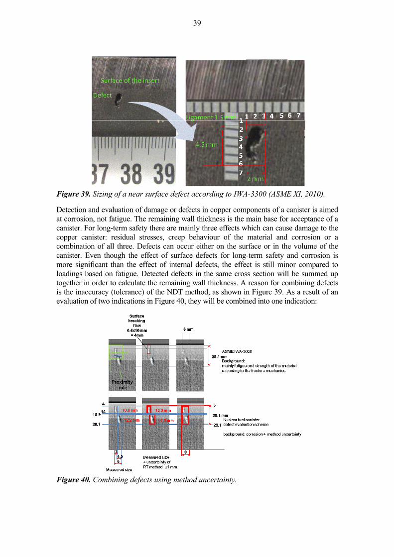
These procedure and figures show how to measure a surface or subsurface defect and gives guidance how to apply from NDT gained information to acceptance or rejection of an inspected component. For insert the ASME XI is followed but in copper components, where the acceptance of the component is based on corrosion rate not a fatigue, the combining rules of defects is based on the error of sizing. A subsurface indication shall be considered a surface defect if any portion of the defect is less than 0.4d from the surface of the component nearest the defect. If the nearest surface is clad, S shall be measured to the clad-base metal interface. S is measured as shown in Figure 38. Casting defect seen in Figure 39 is sized according to the IWA-3300: Real size of the defect is a x l = 4.5 mm x 2mm, but because the ligament is only 1.5 mm and less than 0.4 x 4.5 = 1.8 mm, The ligament should calculate additionally to defect depth so the defect dimensions which should be reported are a x l = 6 mm x 2 mm. This near surface defect (porosity) was detected in Posiva's inspections in nodular cast iron component.
39
Figure 39. Sizing of a near surface defect according to IWA-3300 (ASME XI, 2010).
Detection and evaluation of damage or defects in copper components of a canister is aimed at corrosion, not fatigue. The remaining wall thickness is the main base for acceptance of a canister. For long-term safety there are mainly three effects which can cause damage to the copper canister: residual stresses, creep behaviour of the material and corrosion or a combination of all three. Defects can occur either on the surface or in the volume of the canister. Even though the effect of surface defects for long-term safety and corrosion is more significant than the effect of internal defects, the effect is still minor compared to loadings based on fatigue. Detected defects in the same cross section will be summed up together in order to calculate the remaining wall thickness. A reason for combining defects is the inaccuracy (tolerance) of the NDT method, as shown in Figure 39. As a result of an evaluation of two indications in Figure 40, they will be combined into one indication:
Figure 40. Combining defects using method uncertainty.
40
In depth direction, which is the most important direction for the remaining wall thickness, the combining of defects determines the inaccuracy of the used NDT method in depth sizing. The final result for combining defects can be related to the specific defect analysis of the detected defect. In length direction the combining distance in ASME XI varies depending on the defect type and position. The rule for combining in length direction can also be applied similarly.
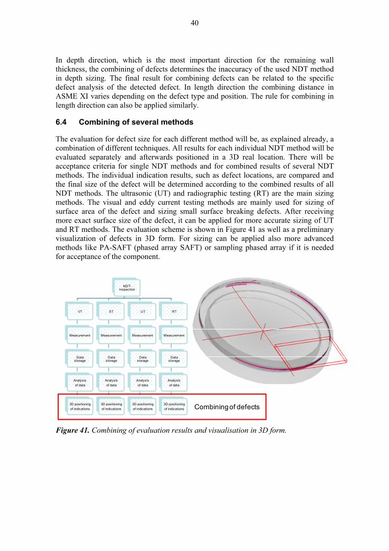
6.4 Combining of several methods
The evaluation for defect size for each different method will be, as explained already, a combination of different techniques. All results for each individual NDT method will be evaluated separately and afterwards positioned in a 3D real location. There will be acceptance criteria for single NDT methods and for combined results of several NDT methods. The individual indication results, such as defect locations, are compared and the final size of the defect will be determined according to the combined results of all NDT methods. The ultrasonic (UT) and radiographic testing (RT) are the main sizing methods. The visual and eddy current testing methods are mainly used for sizing of surface area of the defect and sizing small surface breaking defects. After receiving more exact surface size of the defect, it can be applied for more accurate sizing of UT and RT methods. The evaluation scheme is shown in Figure 41 as well as a preliminary visualization of defects in 3D form. For sizing can be applied also more advanced methods like PA-SAFT (phased array SAFT) or sampling phased array if it is needed for acceptance of the component.
NDT-Inspection
VT
Measurement
Datastorage
Analysis
of data
3D positioning
of indications
ET
Measurement
Datastorage
Analysis
of data
3D positioning
of indications
UT
Measurement
Datastorage
Analysis
of data
3D positioning
of indications
RT
Measurement
Datastorage
Analysis
of data
3D positioning
of indications Combiningof defects
Figure 41. Combining of evaluation results and visualisation in 3D form.
41
7 PRIMARY ACCEPTANCE / REJECTION METHODS
Primary acceptance methods are ultrasonic testing and radiographic testing. The main acceptance is based on the normal NDT inspection result. In case of indications exceed the preliminary acceptance criteria acceptance and rejection is based on the sizing of the defects and regarding to the results of these sizing procedures the component, weld are accepted or rejected. The acceptance - rejection process based on the NDT results is shown in Figure 22.

42
43
8 SUPPORTIVE ACCEPTANCE / REJECTION METHODS
Supportive methods are surface methods: remote visual camera inspection and eddy current inspection. The information given from surface defects by these surface methods are defect accurate location and surface size. In some cases results of eddy current testing can be used as base for rejection. Eddy current testing can also be used for detection of handling and transport defects and sizing these types of defects as well for weld surface defect detection. Allowable further repair actions for smaller surface defects.

44

45
9 ALLOWABLE FURTHER REPAIR ACTIONS FOR SMALLER SURFACE DEFECTS
The allowable repair action is removal of surface defects by smooth grinding. The limit for acceptable removal has been presented in table, which is possible until to 5 mm depth continuously along the weld (10% from the nominal wall thickness). The intact material in the grinded position should be at least 35 mm. This means that the grinded position can contain also internal defects like root defects, cavities or wormholes but their combined size is less than 8.5 mm if the minimum wall thickness is 48.5 mm. 35 mm (allowable remaining wall thickness) +8.5 mm (maximum combined internal defect depth) + 5 mm (maximum allowable grinded thickness) = 48.5 mm. The minimum wall thickness is 48.5 according to the drawings. In case when the minimum wall thickness is 50 mm the maximum combined internal defect depth can be 10 mm.

46
47
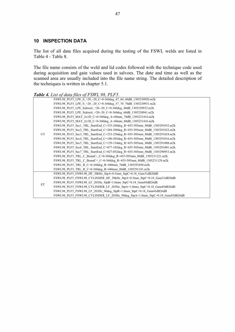
10 INSPECTION DATA
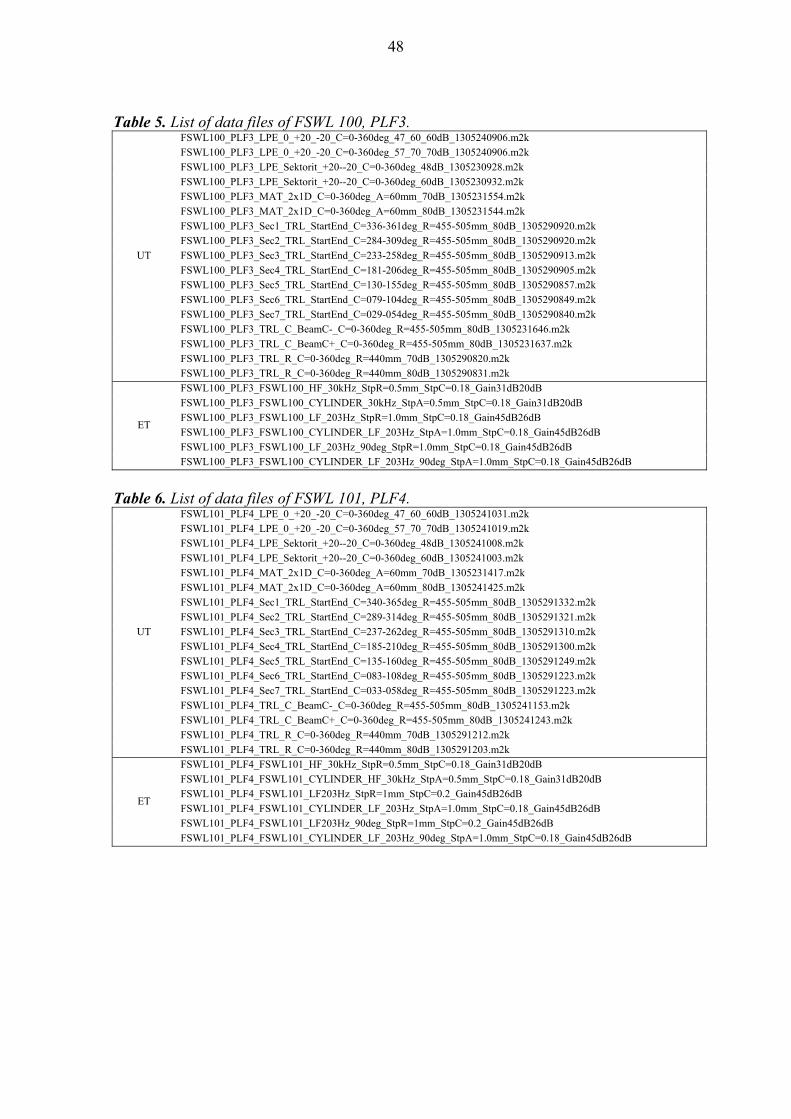
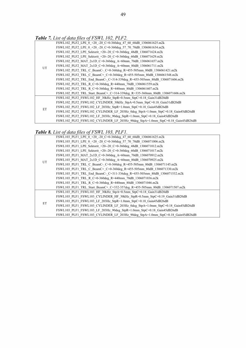
The list of all data files acquired during the testing of the FSWL welds are listed in Table 4 - Table 8. The file name consists of the weld and lid codes followed with the technique code used during acquisition and gain values used in salvoes. The date and time as well as the scanned area are usually included into the file name string. The detailed description of the techniques is written in chapter 5.1. Table 4. List of data files of FSWL 98, PLF5.
UT
FSWL98_PLF5_LPE_0_+20_-20_C=0-360deg_47_60_60dB_1305230920.m2k FSWL98_PLF5_LPE_0_+20_-20_C=0-360deg_57_70_70dB_1305230931.m2k
FSWL98_PLF5_LPE_Sektorit_+20--20_C=0-360deg_48dB_1305230932.m2k
FSWL98_PLF5_LPE_Sektorit_+20--20_C=0-360deg_60dB_1305230941.m2k FSWL98_PLF5_MAT_2x1D_C=0-360deg_A=60mm_70dB_1305231416.m2k
FSWL98_PLF5_MAT_2x1D_C=0-360deg_A=60mm_80dB_1305231416.m2k
FSWL98_PLF5_Sec1_TRL_StartEnd_C=335-260deg_R=455-505mm_80dB_1305291032.m2k FSWL98_PLF5_Sec2_TRL_StartEnd_C=284-309deg_R=455-505mm_80dB_1305291032.m2k
FSWL98_PLF5_Sec3_TRL_StartEnd_C=233-258deg_R=455-505mm_80dB_1305291024.m2k
FSWL98_PLF5_Sec4_TRL_StartEnd_C=180-205deg_R=455-505mm_80dB_1305291016.m2k FSWL98_PLF5_Sec5_TRL_StartEnd_C=129-154deg_R=455-505mm_80dB_1305291008.m2k
FSWL98_PLF5_Sec6_TRL_StartEnd_C=077-102deg_R=455-505mm_80dB_1305291001.m2k FSWL98_PLF5_Sec7_TRL_StartEnd_C=027-052deg_R=455-505mm_80dB_1305290953.m2k
FSWL98_PLF5_TRL_C_BeamC-_C=0-360deg_R=455-505mm_80dB_1305231221.m2k
FSWL98_PLF5_TRL_C_BeamC+_C=0-360deg_R=455-505mm_80dB_1305231129.m2k FSWL98_PLF5_TRL_R_C=0-360deg_R=440mm_70dB_1305291050.m2k
FSWL98_PLF5_TRL_R_C=0-360deg_R=440mm_80dB_1305291101.m2k
ET
FSWL98_PLF5_FSWL98_HF_30kHz_StpA=0.5mm_StpC=0.18_Gain31dB20dB FSWL98_PLF5_FSWL98_CYLINDER_HF_30kHz_StpA=0.5mm_StpC=0.18_Gain31dB20dB
FSWL98_PLF5_FSWL98_LF_203Hz_StpR=1.0mm_StpC=0.18_Gain45dB26dB
FSWL98_PLF5_FSWL98_CYLINDER_LF_203Hz_StpA=1.0mm_StpC=0.18_Gain45dB26dB FSWL98_PLF5_FSWL98_LF_203Hz_90deg_StpR=1.0mm_StpC=0.18_Gain45dB26dB
FSWL98_PLF5_FSWL98_CYLINDER_LF_203Hz_90deg_StpA=1.0mm_StpC=0.18_Gain45dB26dB
48
Table 5. List of data files of FSWL 100, PLF3.
UT
FSWL100_PLF3_LPE_0_+20_-20_C=0-360deg_47_60_60dB_1305240906.m2k FSWL100_PLF3_LPE_0_+20_-20_C=0-360deg_57_70_70dB_1305240906.m2k
FSWL100_PLF3_LPE_Sektorit_+20--20_C=0-360deg_48dB_1305230928.m2k
FSWL100_PLF3_LPE_Sektorit_+20--20_C=0-360deg_60dB_1305230932.m2k FSWL100_PLF3_MAT_2x1D_C=0-360deg_A=60mm_70dB_1305231554.m2k
FSWL100_PLF3_MAT_2x1D_C=0-360deg_A=60mm_80dB_1305231544.m2k
FSWL100_PLF3_Sec1_TRL_StartEnd_C=336-361deg_R=455-505mm_80dB_1305290920.m2k FSWL100_PLF3_Sec2_TRL_StartEnd_C=284-309deg_R=455-505mm_80dB_1305290920.m2k
FSWL100_PLF3_Sec3_TRL_StartEnd_C=233-258deg_R=455-505mm_80dB_1305290913.m2k
FSWL100_PLF3_Sec4_TRL_StartEnd_C=181-206deg_R=455-505mm_80dB_1305290905.m2k FSWL100_PLF3_Sec5_TRL_StartEnd_C=130-155deg_R=455-505mm_80dB_1305290857.m2k
FSWL100_PLF3_Sec6_TRL_StartEnd_C=079-104deg_R=455-505mm_80dB_1305290849.m2k
FSWL100_PLF3_Sec7_TRL_StartEnd_C=029-054deg_R=455-505mm_80dB_1305290840.m2k FSWL100_PLF3_TRL_C_BeamC-_C=0-360deg_R=455-505mm_80dB_1305231646.m2k
FSWL100_PLF3_TRL_C_BeamC+_C=0-360deg_R=455-505mm_80dB_1305231637.m2k
FSWL100_PLF3_TRL_R_C=0-360deg_R=440mm_70dB_1305290820.m2k FSWL100_PLF3_TRL_R_C=0-360deg_R=440mm_80dB_1305290831.m2k
ET
FSWL100_PLF3_FSWL100_HF_30kHz_StpR=0.5mm_StpC=0.18_Gain31dB20dB
FSWL100_PLF3_FSWL100_CYLINDER_30kHz_StpA=0.5mm_StpC=0.18_Gain31dB20dB FSWL100_PLF3_FSWL100_LF_203Hz_StpR=1.0mm_StpC=0.18_Gain45dB26dB
FSWL100_PLF3_FSWL100_CYLINDER_LF_203Hz_StpA=1.0mm_StpC=0.18_Gain45dB26dB
FSWL100_PLF3_FSWL100_LF_203Hz_90deg_StpR=1.0mm_StpC=0.18_Gain45dB26dB FSWL100_PLF3_FSWL100_CYLINDER_LF_203Hz_90deg_StpA=1.0mm_StpC=0.18_Gain45dB26dB
Table 6. List of data files of FSWL 101, PLF4.
UT
FSWL101_PLF4_LPE_0_+20_-20_C=0-360deg_47_60_60dB_1305241031.m2k
FSWL101_PLF4_LPE_0_+20_-20_C=0-360deg_57_70_70dB_1305241019.m2k FSWL101_PLF4_LPE_Sektorit_+20--20_C=0-360deg_48dB_1305241008.m2k
FSWL101_PLF4_LPE_Sektorit_+20--20_C=0-360deg_60dB_1305241003.m2k
FSWL101_PLF4_MAT_2x1D_C=0-360deg_A=60mm_70dB_1305231417.m2k FSWL101_PLF4_MAT_2x1D_C=0-360deg_A=60mm_80dB_1305241425.m2k
FSWL101_PLF4_Sec1_TRL_StartEnd_C=340-365deg_R=455-505mm_80dB_1305291332.m2k
FSWL101_PLF4_Sec2_TRL_StartEnd_C=289-314deg_R=455-505mm_80dB_1305291321.m2k FSWL101_PLF4_Sec3_TRL_StartEnd_C=237-262deg_R=455-505mm_80dB_1305291310.m2k
FSWL101_PLF4_Sec4_TRL_StartEnd_C=185-210deg_R=455-505mm_80dB_1305291300.m2k
FSWL101_PLF4_Sec5_TRL_StartEnd_C=135-160deg_R=455-505mm_80dB_1305291249.m2k FSWL101_PLF4_Sec6_TRL_StartEnd_C=083-108deg_R=455-505mm_80dB_1305291223.m2k
FSWL101_PLF4_Sec7_TRL_StartEnd_C=033-058deg_R=455-505mm_80dB_1305291223.m2k
FSWL101_PLF4_TRL_C_BeamC-_C=0-360deg_R=455-505mm_80dB_1305241153.m2k FSWL101_PLF4_TRL_C_BeamC+_C=0-360deg_R=455-505mm_80dB_1305241243.m2k
FSWL101_PLF4_TRL_R_C=0-360deg_R=440mm_70dB_1305291212.m2k
FSWL101_PLF4_TRL_R_C=0-360deg_R=440mm_80dB_1305291203.m2k
ET
FSWL101_PLF4_FSWL101_HF_30kHz_StpR=0.5mm_StpC=0.18_Gain31dB20dB
FSWL101_PLF4_FSWL101_CYLINDER_HF_30kHz_StpA=0.5mm_StpC=0.18_Gain31dB20dB FSWL101_PLF4_FSWL101_LF203Hz_StpR=1mm_StpC=0.2_Gain45dB26dB
FSWL101_PLF4_FSWL101_CYLINDER_LF_203Hz_StpA=1.0mm_StpC=0.18_Gain45dB26dB
FSWL101_PLF4_FSWL101_LF203Hz_90deg_StpR=1mm_StpC=0.2_Gain45dB26dB FSWL101_PLF4_FSWL101_CYLINDER_LF_203Hz_90deg_StpA=1.0mm_StpC=0.18_Gain45dB26dB
49
Table 7. List of data files of FSWL 102, PLF2.
UT
FSWL102_PLF2_LPE_0_+20_-20_C=0-360deg_47_60_60dB_1306061625.m2k
FSWL102_PLF2_LPE_0_+20_-20_C=0-360deg_57_70_70dB_1306061634.m2k
FSWL102_PLF2_LPE_Sektorit_+20--20_C=0-360deg_48dB_1306071624.m2k
FSWL102_PLF2_LPE_Sektorit_+20--20_C=0-360deg_60dB_1306071629.m2k FSWL102_PLF2_MAT_2x1D_C=0-360deg_A=60mm_70dB_1306061657.m2k
FSWL102_PLF2_MAT_2x1D_C=0-360deg_A=60mm_80dB_1306061711.m2k
FSWL102_PLF2_TRL_C_BeamC-_C=0-360deg_R=455-505mm_80dB_1306061421.m2k FSWL102_PLF2_TRL_C_BeamC+_C=0-360deg_R=455-505mm_80dB_1306061548.m2k
FSWL102_PLF2_TRL_End_BeamC-_C=314-339deg_R=455-505mm_80dB_1306071606.m2k
FSWL102_PLF2_TRL_R_C=0-360deg_R=440mm_70dB_1306061559.m2k FSWL102_PLF2_TRL_R_C=0-360deg_R=440mm_80dB_1306061607.m2k
FSWL102_PLF2_TRL_Start_BeamC+_C=314-339deg_R=335-360mm_80dB_1306071606.m2k
ET
FSWL102_PLF2_FSWL102_HF_30kHz_StpR=0.5mm_StpC=0.18_Gain31dB20dB FSWL102_PLF2_FSWL102_CYLINDER_30kHz_StpA=0.5mm_StpC=0.18_Gain31dB20dB
FSWL102_PLF2_FSWL102_LF_203Hz_StpR=1.0mm_StpC=0.18_Gain45dB26dB
FSWL102_PLF2_FSWL102_CYLINDER_LF_203Hz_0deg_StpA=1.0mm_StpC=0.18_Gain45dB26dB FSWL102_PLF2_FSWL102_LF_203Hz_90deg_StpR=1.0mm_StpC=0.18_Gain45dB26dB
FSWL102_PLF2_FSWL102_CYLINDER_LF_203Hz_90deg_StpA=1.0mm_StpC=0.18_Gain45dB26dB
Table 8. List of data files of FSWL 103, PLF1.
UT
FSWL103_PLF1_LPE_0_+20_-20_C=0-360deg_47_60_60dB_1306061625.m2k
FSWL103_PLF1_LPE_0_+20_-20_C=0-360deg_57_70_70dB_1306071006.m2k
FSWL103_PLF1_LPE_Sektorit_+20--20_C=0-360deg_48dB_1306071012.m2k
FSWL103_PLF1_LPE_Sektorit_+20--20_C=0-360deg_60dB_1306071017.m2k FSWL103_PLF1_MAT_2x1D_C=0-360deg_A=60mm_70dB_1306070912.m2k
FSWL103_PLF1_MAT_2x1D_C=0-360deg_A=60mm_80dB_1306070925.m2k
FSWL103_PLF1_TRL_C_BeamC-_C=0-360deg_R=455-505mm_80dB_1306071145.m2k FSWL103_PLF1_TRL_C_BeamC+_C=0-360deg_R=455-505mm_80dB_1306071330.m2k
FSWL103_PLF1_TRL_End_BeamC-_C=311-336deg_R=455-505mm_80dB_1306071532.m2k
FSWL103_PLF1_TRL_R_C=0-360deg_R=440mm_70dB_1306071036.m2k FSWL103_PLF1_TRL_R_C=0-360deg_R=440mm_80dB_1306071046.m2k
FSWL103_PLF1_TRL_Start_BeamC+_C=332-357deg_R=455-505mm_80dB_1306071507.m2k
ET
FSWL103_PLF1_FSWL103_HF_30kHz_StpA=0.5mm_StpC=0.18_Gain31dB20dB FSWL103_PLF1_FSWL103_CYLINDER_HF_30kHz_StpR=0.5mm_StpC=0.19_Gain31dB20dB
FSWL103_PLF1_FSWL103_LF_203Hz_StpR=1.0mm_StpC=0.18_Gain45dB26dB
FSWL103_PLF1_FSWL103_CYLINDER_LF_203Hz_0deg_StpA=1.0mm_StpC=0.18_Gain45dB26dB FSWL103_PLF1_FSWL103_LF_203Hz_90deg_StpR=1.0mm_StpC=0.18_Gain45dB26dB
FSWL103_PLF1_FSWL103_CYLINDER_LF_203Hz_90deg_StpA=1.0mm_StpC=0.18_Gain45dB26dB
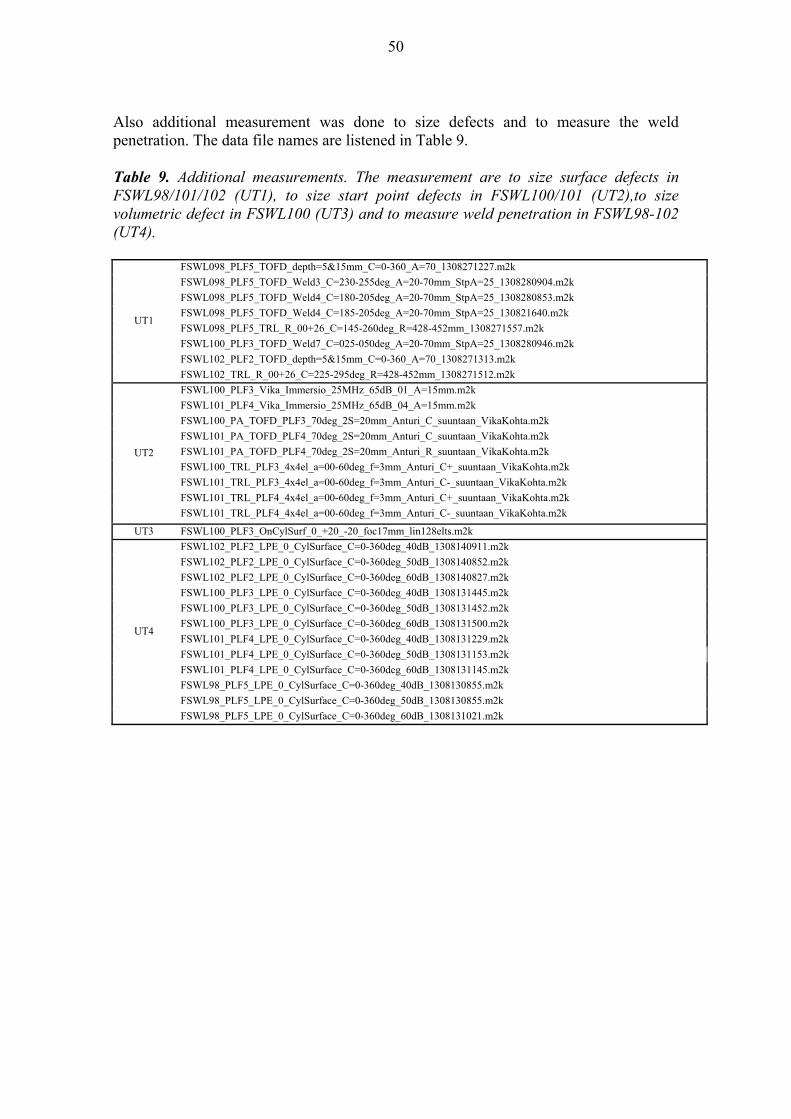
50
Also additional measurement was done to size defects and to measure the weld penetration. The data file names are listened in Table 9. Table 9. Additional measurements. The measurement are to size surface defects in FSWL98/101/102 (UT1), to size start point defects in FSWL100/101 (UT2),to size volumetric defect in FSWL100 (UT3) and to measure weld penetration in FSWL98-102 (UT4).
UT1
FSWL098_PLF5_TOFD_depth=5&15mm_C=0-360_A=70_1308271227.m2k
FSWL098_PLF5_TOFD_Weld3_C=230-255deg_A=20-70mm_StpA=25_1308280904.m2k
FSWL098_PLF5_TOFD_Weld4_C=180-205deg_A=20-70mm_StpA=25_1308280853.m2k
FSWL098_PLF5_TOFD_Weld4_C=185-205deg_A=20-70mm_StpA=25_130821640.m2k
FSWL098_PLF5_TRL_R_00+26_C=145-260deg_R=428-452mm_1308271557.m2k
FSWL100_PLF3_TOFD_Weld7_C=025-050deg_A=20-70mm_StpA=25_1308280946.m2k
FSWL102_PLF2_TOFD_depth=5&15mm_C=0-360_A=70_1308271313.m2k
FSWL102_TRL_R_00+26_C=225-295deg_R=428-452mm_1308271512.m2k
UT2
FSWL100_PLF3_Vika_Immersio_25MHz_65dB_01_A=15mm.m2k
FSWL101_PLF4_Vika_Immersio_25MHz_65dB_04_A=15mm.m2k
FSWL100_PA_TOFD_PLF3_70deg_2S=20mm_Anturi_C_suuntaan_VikaKohta.m2k
FSWL101_PA_TOFD_PLF4_70deg_2S=20mm_Anturi_C_suuntaan_VikaKohta.m2k
FSWL101_PA_TOFD_PLF4_70deg_2S=20mm_Anturi_R_suuntaan_VikaKohta.m2k
FSWL100_TRL_PLF3_4x4el_a=00-60deg_f=3mm_Anturi_C+_suuntaan_VikaKohta.m2k
FSWL101_TRL_PLF3_4x4el_a=00-60deg_f=3mm_Anturi_C-_suuntaan_VikaKohta.m2k
FSWL101_TRL_PLF4_4x4el_a=00-60deg_f=3mm_Anturi_C+_suuntaan_VikaKohta.m2k
FSWL101_TRL_PLF4_4x4el_a=00-60deg_f=3mm_Anturi_C-_suuntaan_VikaKohta.m2k
UT3 FSWL100_PLF3_OnCylSurf_0_+20_-20_foc17mm_lin128elts.m2k
UT4
FSWL102_PLF2_LPE_0_CylSurface_C=0-360deg_40dB_1308140911.m2k
FSWL102_PLF2_LPE_0_CylSurface_C=0-360deg_50dB_1308140852.m2k
FSWL102_PLF2_LPE_0_CylSurface_C=0-360deg_60dB_1308140827.m2k
FSWL100_PLF3_LPE_0_CylSurface_C=0-360deg_40dB_1308131445.m2k
FSWL100_PLF3_LPE_0_CylSurface_C=0-360deg_50dB_1308131452.m2k
FSWL100_PLF3_LPE_0_CylSurface_C=0-360deg_60dB_1308131500.m2k
FSWL101_PLF4_LPE_0_CylSurface_C=0-360deg_40dB_1308131229.m2k
FSWL101_PLF4_LPE_0_CylSurface_C=0-360deg_50dB_1308131153.m2k
FSWL101_PLF4_LPE_0_CylSurface_C=0-360deg_60dB_1308131145.m2k
FSWL98_PLF5_LPE_0_CylSurface_C=0-360deg_40dB_1308130855.m2k
FSWL98_PLF5_LPE_0_CylSurface_C=0-360deg_50dB_1308130855.m2k
FSWL98_PLF5_LPE_0_CylSurface_C=0-360deg_60dB_1308131021.m2k
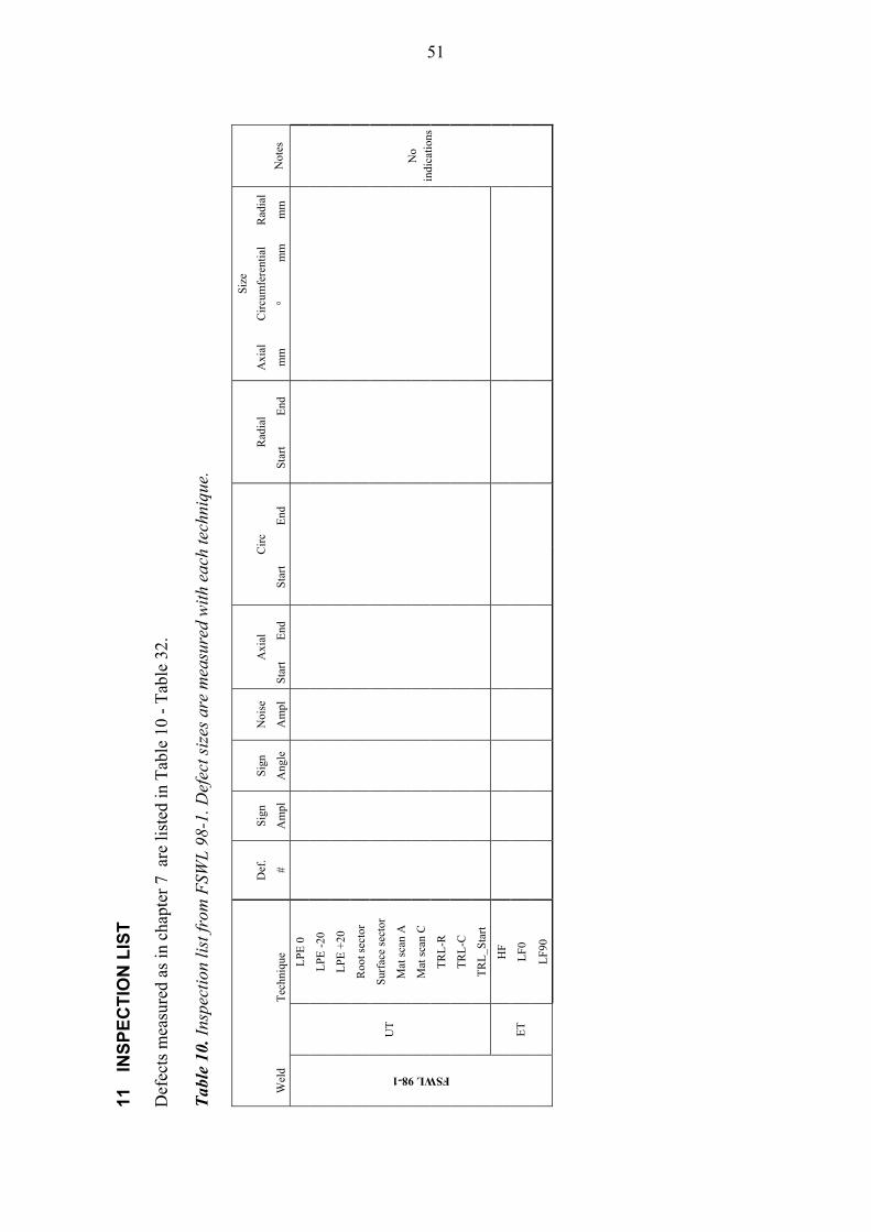
11
INS
PE
CT
ION
LIS
T
Def
ects
mea
sure
d as
in c
hapt
er 7
are
list
ed in
Tab
le 1
0 -
Tab
le 3
2.
Tab
le 1
0. I
nspe
ctio
n li
st fr
om F
SWL
98-
1. D
efec
t siz
es a
re m
easu
red
wit
h ea
ch te
chni
que.
S
ize
Def
. S
ign
Sig
n N
oise
A
xial
C
irc
Rad
ial
Axi
al
Cir
cum
fere
ntia
l R
adia
l
Wel
d T
echn
ique
#
Am
pl
Ang
le
Am
pl
Sta
rtE
nd
Sta
rt
End
S
tart
E
nd
mm
°
mm
m
m
Not
es
FSWL 98-1
UT
LP
E 0
No
indi
cati
ons
LP
E -
20
LP
E +
20
Roo
t sec
tor
Sur
face
sec
tor
Mat
sca
n A
Mat
sca
n C
TR
L-R
TR
L-C
TR
L_S
tart
ET
HF
LF
0
LF
90
51
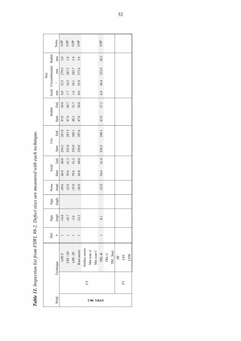
Tab
le 1
1. I
nspe
ctio
n li
st fr
om F
SWL
98-
2. D
efec
t siz
es a
re m
easu
red
wit
h ea
ch te
chni
que.
S
ize
Def
. S
ign
Sig
n N
oise
A
xial
C
irc
Rad
ial
Axi
alC
ircu
mfe
rent
ial
Rad
ial
Wel
d T
echn
ique
#
Am
pl
Ang
le
Am
pl
Sta
rt
End
S
tart
E
nd
Sta
rt
End
m
m
° m
m
mm
N
otes
FSWL 98-2
UT
LP
E 0
1
-14.
8
-29.
6 60
.0
60.0
25
4.3
287.
8 47
.0
50.0
0.
0 33
.5
279.
5 3.
0 L
OP
LP
E +
20
1 -1
0.7
-2
3.0
59.6
61
.3
253.
0 28
7.5
47.9
49
.7
1.7
34.5
28
7.3
1.8
LO
P
LP
E -
20
1 -3
.6
-2
5.0
59.6
61
.2
254.
0 28
8.1
48.3
51
.7
1.6
34.1
28
3.7
3.4
LO
P
Roo
t sec
tor
1 -1
2.2
-2
6.0
60.0
60
.0
254.
8 28
7.6
47.0
50
.0
0.0
32.8
27
3.6
3.0
LO
P
Sur
face
sec
tor
Mat
sca
n A
Mat
sca
n C
TR
L-R
1
-8.1
-23.
0 54
.4
61.4
25
4.5
290.
1 47
.0
57.2
6.
9 30
.4
253.
9 10
.3
LO
P
TR
L-C
TR
L_S
tart
ET
HF
LF
0
LF
90
52
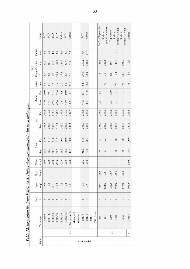
Tab
le 1
2. I
nspe
ctio
n li
st fr
om F
SWL
98-
3. D
efec
t siz
es a
re m
easu
red
wit
h ea
ch te
chni
que.
Siz
e
Def
. S
ign
Sig
n N
oise
A
xial
C
irc
Rad
ial
Axi
alC
ircu
mfe
rent
ial
Rad
ial
Wel
d T
echn
ique
#
Am
pl
Ang
le
Am
pl
Sta
rt
End
S
tart
E
nd
Sta
rt
End
m
m
° m
m
mm
N
otes
FSWL 98-3
UT
LP
E 0
1
-13.
3
-30.
0 61
.0
61.0
20
3.4
209.
8 48
.0
50.0
0.
0 6.
4 53
.3
2.0
LO
P
LP
E +
20
1 -1
0.2
-2
2.0
60.7
61
.4
203.
7 21
0.5
47.3
49
.1
0.7
6.8
56.7
1.
8 L
OP
LP
E -
20
1 -1
.3
-2
2.0
60.3
61
.8
205.
0 21
3.6
47.5
51
.5
1.5
8.6
71.7
4.
0 L
OP
LP
E -
20
2 -1
1.7
-2
2.0
60.3
61
.7
216.
7 23
7.0
47.6
52
.6
1.4
20.3
16
9.1
5.0
LO
P
LP
E -
20
3 -1
0.2
-2
3.0
68.3
70
.4
202.
0 23
9.6
-3.6
4.
4 2.
1 37
.6
346.
9 8.
0 S
urfa
ce
Roo
t sec
tor
1 -1
0.4
-2
5.0
60.0
60
.0
203.
6 21
0.0
46.9
50
.0
0.0
6.4
53.4
3.
1 L
OP
Sur
face
sec
tor
4 -7
.1
-2
6.0
17.5
38
.0
243.
4 24
9.2
1.3
3.6
20.5
5.
8 53
.0
2.3
Sur
face
Mat
sca
n A
Mat
sca
n C
TR
L-R
1
-10.
1
-25.
2 55
.3
61.8
20
6.0
233.
6 47
.2
55.1
6.
5 27
.6
230.
2 7.
9 L
OP
TR
L-R
3
-7.5
-25.
6 63
.6
78.3
20
5.7
238.
5 -0
.7
11.0
14
.7
32.8
30
1.2
11.7
S
urfa
ce
TR
L-C
TR
L_S
tart
ET
HF
4
7191
35
.3
0
71
238.
0 25
4.1
0.0
2.0
-
16
146.
6 -
Sur
face
/Top
sur
face
HF
3
5248
2 7.
5
67
73
205.
0 23
8.0
- -
70
33
302.
4 -
Sur
face
(W
idth
=2.
2mm
)
LF
0 4
7202
8 33
.7
-
-
251.
7 25
7.2
0.0
12.0
-
5.
5 50
.4
- T
op s
urfa
ce
LF
0 4
5986
6 42
.5
0
70
236.
5 25
2.5
- -
70
16.0
14
6.6
- S
urfa
ce
(dep
th =
1.5
mm
)
LF
90
3 67
756
45.8
0 70
20
8.8
250.
9 -
- 70
32
.1
294.
0 -
Sur
face
(d
epth
= 1
.7 m
m)
RT
9
MeV
4
1030
0 10
000
8.4
70.9
24
0.2
252.
5 0
71
12.3
11
2,7
Sur
face
53
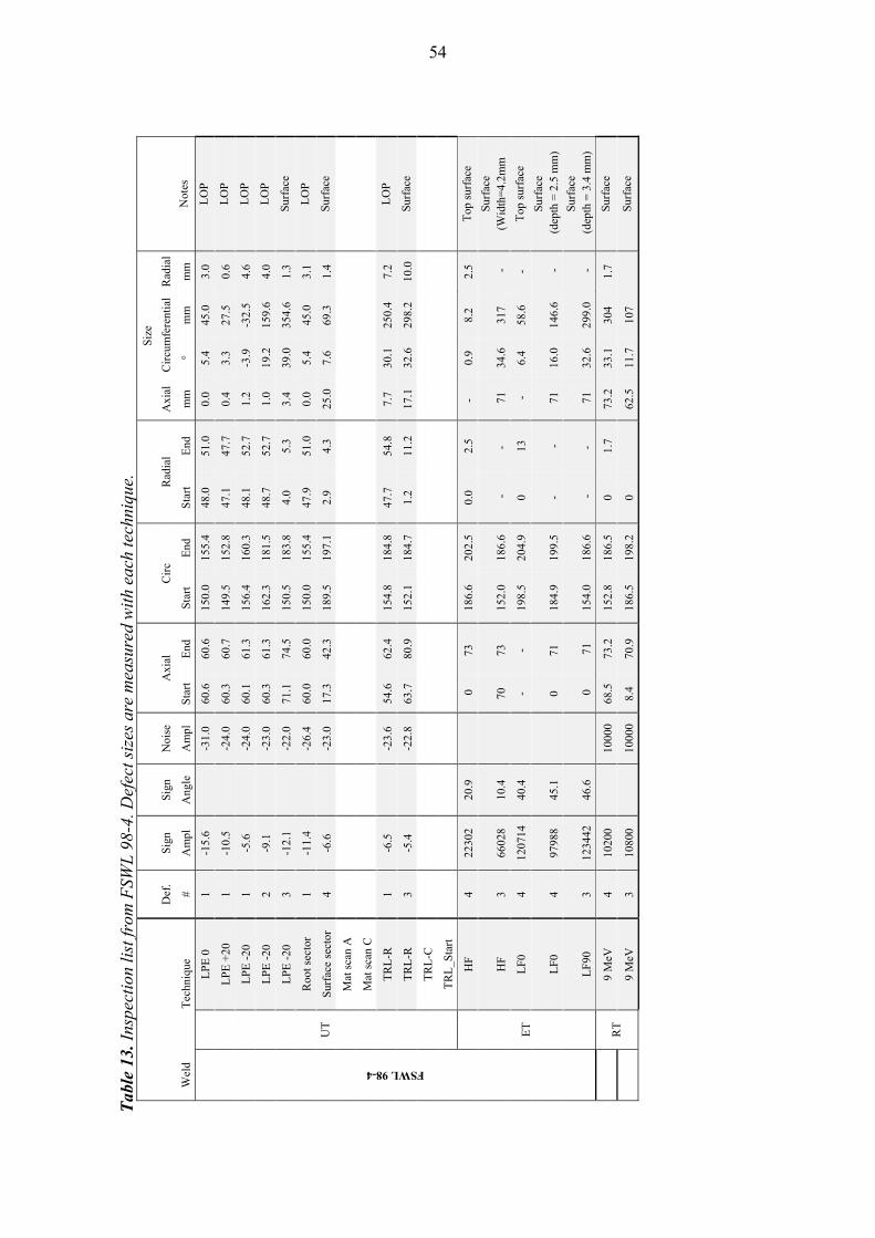
Tab
le 1
3. I
nspe
ctio
n li
st fr
om F
SWL
98-
4. D
efec
t siz
es a
re m
easu
red
wit
h ea
ch te
chni
que.
Siz
e
Def
. S
ign
Sig
n N
oise
A
xial
C
irc
Rad
ial
Axi
al
Cir
cum
fere
ntia
lR
adia
l
Wel
d T
echn
ique
#
Am
pl
Ang
le
Am
pl
Sta
rt
End
S
tart
E
nd
Sta
rt
End
m
m
° m
m
mm
N
otes
FSWL 98-4
UT
LP
E 0
1
-15.
6
-31.
0 60
.6
60.6
15
0.0
155.
4 48
.0
51.0
0.
0 5.
4 45
.0
3.0
LO
P
LP
E +
20
1 -1
0.5
-2
4.0
60.3
60
.7
149.
5 15
2.8
47.1
47
.7
0.4
3.3
27.5
0.
6 L
OP
LP
E -
20
1 -5
.6
-2
4.0
60.1
61
.3
156.
4 16
0.3
48.1
52
.7
1.2
-3.9
-3
2.5
4.6
LO
P
LP
E -
20
2 -9
.1
-2
3.0
60.3
61
.3
162.
3 18
1.5
48.7
52
.7
1.0
19.2
15
9.6
4.0
LO
P
LP
E -
20
3 -1
2.1
-2
2.0
71.1
74
.5
150.
5 18
3.8
4.0
5.3
3.4
39.0
35
4.6
1.3
Sur
face
Roo
t sec
tor
1 -1
1.4
-2
6.4
60.0
60
.0
150.
0 15
5.4
47.9
51
.0
0.0
5.4
45.0
3.
1 L
OP
Sur
face
sec
tor
4 -6
.6
-2
3.0
17.3
42
.3
189.
5 19
7.1
2.9
4.3
25.0
7.
6 69
.3
1.4
Sur
face
Mat
sca
n A
Mat
sca
n C
TR
L-R
1
-6.5
-23.
6 54
.6
62.4
15
4.8
184.
8 47
.7
54.8
7.
7 30
.1
250.
4 7.
2 L
OP
TR
L-R
3
-5.4
-22.
8 63
.7
80.9
15
2.1
184.
7 1.
2 11
.2
17.1
32
.6
298.
2 10
.0
Sur
face
TR
L-C
TR
L_S
tart
ET
HF
4
2230
2 20
.9
0
73
18
6.6
202.
5 0.
0 2.
5 -
0.
9 8.
2 2.
5 T
op s
urfa
ce
HF
3
6602
8 10
.4
70
73
15
2.0
186.
6 -
-
7
1 34
.6
317
-
Sur
face
(W
idth
=4.
2mm
LF
0 4
1207
14
40.4
- -
19
8.5
204.
9 0
13
-
6.4
58.6
-
Top
sur
face
LF
0 4
9798
8 45
.1
0
71
184.
9 19
9.5
-
- 7
1 16
.0
146.
6 -
S
urfa
ce
(de
pth
= 2
.5 m
m)
LF
90
3 12
3442
46
.6
0
71
15
4.0
186.
6 -
-
7
1 32
.6
299.
0 -
S
urfa
ce
(de
pth
= 3
.4 m
m)
RT
9
MeV
4
1020
0 10
000
68.5
73
.2
152.
8 18
6.5
0 1.
7 73
.2
33.1
30
4 1.
7 S
urfa
ce
9 M
eV
3 10
800
1000
0 8.
4 70
.9
186.
5 19
8.2
0 62
.5
11.7
10
7 S
urfa
ce
54
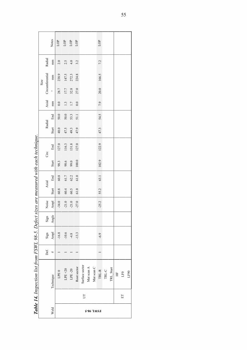
Tab
le 1
4. I
nspe
ctio
n li
st fr
om F
SWL
98-
5. D
efec
t siz
es a
re m
easu
red
wit
h ea
ch te
chni
que.
Siz
e
Def
. S
ign
Sig
n N
oise
A
xial
C
irc
Rad
ial
Axi
al
Cir
cum
fere
ntia
l R
adia
l
Wel
d T
echn
ique
#
Am
pl
Ang
le
Am
pl
Sta
rt
End
S
tart
E
nd
Sta
rt
End
m
m
° m
m
mm
N
otes
FSWL 98-5
UT
LP
E 0
1
-16.
8
-34.
0 60
.8
60.8
98
.3
127.
0 48
.0
50.0
0.
0 28
.7
238.
9 2.
0 L
OP
LP
E +
20
1 -1
0.6
-2
1.0
60.4
61
.7
98.6
11
6.3
47.5
50
.0
1.3
17.7
14
7.5
2.5
LO
P
LP
E -
20
1 -4
.8
-2
1.0
60.5
62
.2
99.0
13
1.8
49.3
53
.3
1.7
32.8
27
2.3
4.0
LO
P
Roo
t sec
tor
1 -1
3.3
-2
7.0
61.0
61
.0
100.
0 12
7.0
47.9
51
.1
0.0
27.0
22
4.8
3.2
LO
P
Sur
face
sec
tor
Mat
sca
n A
Mat
sca
n C
TR
L-R
1
-6.9
-25.
2 55
.2
63.1
10
2.9
122.
9 47
.3
54.5
7.
9 20
.0
166.
5 7.
2 L
OP
TR
L-C
TR
L_S
tart
ET
HF
LF
0
LF
90
55
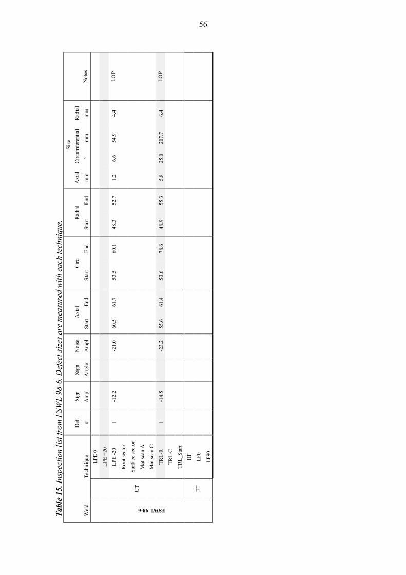
Tab
le 1
5. I
nspe
ctio
n li
st fr
om F
SWL
98-
6. D
efec
t siz
es a
re m
easu
red
wit
h ea
ch te
chni
que.
Siz
e
Def
. S
ign
Sig
n N
oise
A
xial
C
irc
Rad
ial
Axi
al
Cir
cum
fere
ntia
l R
adia
l
Wel
d T
echn
ique
#
Am
pl
Ang
le
Am
pl
Sta
rt
End
S
tart
E
nd
Sta
rt
End
m
m
° m
m
mm
N
otes
FSWL 98-6
UT
LP
E 0
LP
E +
20
LP
E -
20
1 -1
2.2
-2
1.0
60.5
61
.7
53.5
60
.1
48.3
52
.7
1.2
6.6
54.9
4.
4 L
OP
Roo
t sec
tor
Sur
face
sec
tor
Mat
sca
n A
Mat
sca
n C
TR
L-R
1
-14.
5
-23.
2 55
.6
61.4
53
.6
78.6
48
.9
55.3
5.
8 25
.0
207.
7 6.
4 L
OP
TR
L-C
TR
L_S
tart
ET
HF
LF
0
LF
90
56
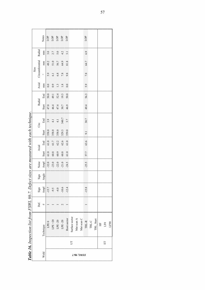
Tab
le 1
6. I
nspe
ctio
n li
st fr
om F
SWL
98-
7. D
efec
t siz
es a
re m
easu
red
wit
h ea
ch te
chni
que.
Siz
e
Def
. S
ign
Sig
n N
oise
A
xial
C
irc
Rad
ial
Axi
al
Cir
cum
fere
ntia
l R
adia
l
Wel
d T
echn
ique
#
Am
pl
Ang
le
Am
pl
Sta
rt
End
S
tart
E
nd
Sta
rt
End
m
m
° m
m
mm
N
otes
FSWL 98-7
UT
LP
E 0
1
-15.
7
-32.
0 61
.0
61.0
35
8.0
3.9
47.0
50
.0
0.0
5.9
49.2
3.
0 L
OP
LP
E +
20
1 -9
.5
-2
3.0
60.8
61
.7
358.
0 4.
1 46
.4
49.1
0.
9 6.
1 51
.0
2.7
LO
P
LP
E -
20
1 -4
.0
-2
2.0
60.9
62
.2
358.
0 4.
1 47
.4
52.4
1.
3 6.
8 56
.7
5.0
LO
P
LP
E -
20
2 -1
0.6
-2
1.0
60.8
62
.6
329.
3 34
0.7
30.7
19
.3
1.8
7.8
64.9
4.
2 L
OP
Roo
t sec
tor
1 -1
2.4
-2
4.5
61.0
61
.0
359.
0 3.
7 46
.9
50.0
0.
0 9.
8 81
.8
3.1
LO
P
Sur
face
sec
tor
Mat
sca
n A
Mat
sca
n C
TR
L-R
1
-15.
8
-25.
5 57
.7
63.6
9.
1 30
.7
49.4
56
.3
5.9
7.8
64.7
6.
9 L
OP
TR
L-C
TR
L_S
tart
ET
HF
LF
0
LF
90
57

Tab
le 1
7. I
nspe
ctio
n li
st fr
om F
SWL
100
-1. D
efec
t siz
es a
re m
easu
red
wit
h ea
ch te
chni
que.
Siz
e
Def
. S
ign
Sig
n N
oise
A
xial
C
irc
Rad
ial
Axi
al
Cir
cum
fere
ntia
l R
adia
l
Wel
d T
echn
ique
#
Am
pl
Ang
le
Am
pl
Sta
rt
End
S
tart
E
nd
Sta
rt
End
m
m
° m
m
mm
N
otes
FSWL 100-1
UT
LP
E 0
LP
E +
20
LP
E -
20
1 -9
.5
-1
9.2
60.3
60
.4
322.
3 32
3.3
49.0
50
.7
0.1
1.0
8.3
1.7
LO
P
LP
E -
20
1(2)
-9
.2
-1
9.6
60.7
61
.3
318.
8 31
9.5
48.7
51
.7
0.6
0.7
5.8
3.0
LO
P
Roo
t sec
tor
Sur
face
sec
tor
Mat
sca
n A
Mat
sca
n C
TR
L-R
1
-10.
9
-27.
0 55
.6
62.4
30
9.7
325.
8 48
.9
54.8
6.
8 16
.1
133.
8 6.
0 L
OP
TR
L-C
TR
L_S
tart
ET
HF
LF
0
LF
90
58
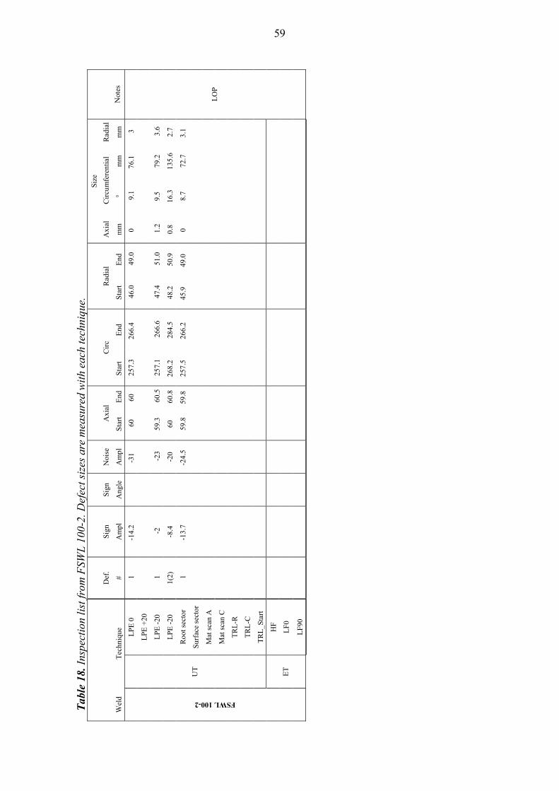
Tab
le 1
8. I
nspe
ctio
n li
st fr
om F
SWL
100
-2. D
efec
t siz
es a
re m
easu
red
wit
h ea
ch te
chni
que.
Siz
e
Def
. S
ign
Sig
n N
oise
A
xial
C
irc
Rad
ial
Axi
al
Cir
cum
fere
ntia
l R
adia
l
Wel
d T
echn
ique
#
Am
pl
Ang
le
Am
pl
Sta
rt
End
S
tart
E
nd
Sta
rt
End
m
m
° m
m
mm
N
otes
FSWL 100-2
UT
LP
E 0
1
-1
4.2
-31
6
0 60
2
57.3
26
6.4
4
6.0
49.
0 0
9
.1
76.1
3
LO
P
LP
E +
20
LP
E -
20
1
-2
-
23
59.3
6
0.5
257
.1
266
.6
47.
4 5
1.0
1.2
9.
5 79
.2
3.6
LP
E -
20
1(2)
-8
.4
-2
0 60
60
.8
268.
2 28
4.5
48.2
50
.9
0.8
16.3
13
5.6
2.7
Roo
t sec
tor
1
-13.
7
-2
4.5
59
.8
59.8
25
7.5
266.
2
45.9
49
.0
0
8.7
72.7
3.
1
Sur
face
sec
tor
Mat
sca
n A
Mat
sca
n C
TR
L-R
TR
L-C
TR
L_S
tart
ET
HF
LF
0
LF
90
59
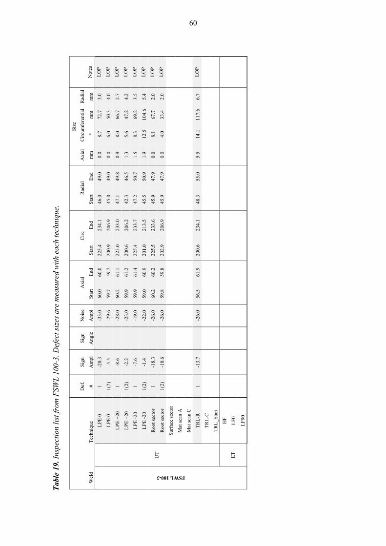
Tab
le 1
9. I
nspe
ctio
n li
st fr
om F
SWL
100
-3. D
efec
t siz
es a
re m
easu
red
wit
h ea
ch te
chni
que.
S
ize
Def
. S
ign
Sig
n N
oise
A
xial
C
irc
Rad
ial
Axi
al
Cir
cum
fere
ntia
l R
adia
l
Wel
d T
echn
ique
#
Am
pl
Ang
le
Am
pl
Sta
rt
End
S
tart
E
nd
Sta
rt
End
m
m
° m
m
mm
N
otes
FSWL 100-3
UT
LP
E 0
1
-20.
3
-33.
0 60
.0
60.0
22
5.4
234.
1 46
.0
49.0
0.
0 8.
7 72
.7
3.0
LO
P
LP
E 0
1(
2)
-5.5
-29.
6 59
.7
59.7
20
0.9
206.
9 45
.0
49.0
0.
0 6.
0 50
.3
4.0
LO
P
LP
E +
20
1 -8
.6
-2
8.0
60.2
61
.1
225.
0 23
3.0
47.1
49
.8
0.9
8.0
66.7
2.
7 L
OP
LP
E +
20
1(2)
-2
.2
-2
3.0
59.9
61
.2
200.
6 20
6.2
42.3
46
.5
1.3
5.6
47.2
4.
2 L
OP
LP
E -
20
1 -7
.6
-1
9.0
59.9
61
.4
225.
4 23
3.7
47.2
50
.7
1.5
8.3
69.2
3.
5 L
OP
LP
E -
20
1(2)
-1
.4
-2
2.0
59.0
60
.9
201.
0 21
3.5
45.5
50
.9
1.9
12.5
10
4.6
5.4
LO
P
Roo
t sec
tor
1 -1
8.3
-2
6.0
60.2
60
.2
225.
5 23
3.6
45.9
47
.9
0.0
8.1
67.7
2.
0 L
OP
Roo
t sec
tor
1(2)
-1
0.6
-2
6.0
59.8
59
.8
202.
9 20
6.9
45.9
47
.9
0.0
4.0
33.4
2.
0 L
OP
Sur
face
sec
tor
Mat
sca
n A
Mat
sca
n C
TR
L-R
1
-13.
7
-26.
0 56
.5
61.9
20
0.6
234.
1 48
.3
55.0
5.
5 14
.1
117.
6 6.
7 L
OP
TR
L-C
TR
L_S
tart
ET
HF
LF
0
LF
90
60
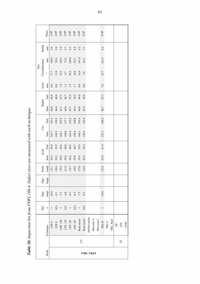
Tab
le 2
0. I
nspe
ctio
n li
st fr
om F
SWL
100
-4. D
efec
t siz
es a
re m
easu
red
wit
h ea
ch te
chni
que.
S
ize
Def
. S
ign
Sig
n N
oise
A
xial
C
irc
Rad
ial
Axi
al
Cir
cum
fere
ntia
l R
adia
l
Wel
d T
echn
ique
#
Am
pl
Ang
le
Am
pl
Sta
rt
End
S
tart
E
nd
Sta
rt
End
m
m
° m
m
mm
N
otes
FSWL 100-4
UT
LP
E 0
1
-10.
8
-32.
1 59
.4
59.4
16
5.7
183.
4 46
.0
49.0
0.
0 17
.7
148.
0 3.
0 L
OP
LP
E 0
1(
2)
-9.1
-30.
4 59
.5
59.5
14
8.9
159.
9 46
.0
49.0
0.
0 11
.0
92.0
3.
0 L
OP
LP
E +
20
1 -7
.3
-1
9.0
59.0
60
.8
168.
7 18
3.0
43.1
47
.5
1.8
14.3
12
0.3
4.4
LO
P
LP
E +
20
1(2)
-4
.8
-2
1.0
59.6
60
.8
149.
0 15
7.7
44.0
46
.7
1.2
8.7
73.0
2.
7 L
OP
LP
E -
20
1 +
4.7
-1
8.7
58.6
60
.5
163.
6 18
3.8
45.7
52
.0
1.9
20.2
16
9.0
6.3
LO
P
LP
E -
20
1(2)
-0
.5
-1
9.0
59.0
60
.7
150.
0 16
0.0
46.5
50
.9
1.7
10.0
83
.5
4.4
LO
P
Roo
t sec
tor
1 -7
.5
-2
7.0
59.4
59
.4
166.
5 18
3.4
44.8
49
.0
0.0
16.9
14
1.6
4.2
LO
P
Roo
t sec
tor
1(2)
-6
.5
-2
4.0
59.4
59
.4
149.
0 15
6.8
45.9
49
.0
0.0
7.8
65.2
3.
1 L
OP
Sur
face
sec
tor
Mat
sca
n A
Mat
sca
n C
TR
L-R
1
-10.
0
-25.
0 55
.8
61.4
15
5.2
180.
8 48
.7
55.3
5.
6 25
.7
213.
4 6.
6 L
OP
TR
L-C
TR
L_S
tart
ET
HF
LF
0
LF
90
61

Tab
le 2
1. I
nspe
ctio
n li
st fr
om F
SWL
100
-5. D
efec
t siz
es a
re m
easu
red
wit
h ea
ch te
chni
que.
S
ize
Def
. S
ign
Sig
n N
oise
A
xial
C
irc
Rad
ial
Axi
al
Cir
cum
fere
ntia
l R
adia
l
Wel
d T
echn
ique
#
Am
pl
Ang
le
Am
pl
Sta
rt
End
S
tart
E
nd
Sta
rt
End
m
m
° m
m
mm
N
otes
FSWL 100-5
UT
LP
E 0
1
-18.
7
-32.
0 59
.7
59.7
98
.2
130.
7 46
.0
49.0
0.
0 32
.5
271.
7 3.
0 L
OP
LP
E +
20
1 -1
1.0
-2
1.0
58.7
60
.1
104.
0 13
0.0
45.0
48
.5
1.4
26.0
21
7.8
3.5
LO
P
LP
E -
20
1 -5
.3
-2
1.0
59.0
60
.3
103.
3 13
1.1
47.5
51
.1
1.3
27.8
23
1.7
3.6
LO
P
Roo
t sec
tor
1 -1
4.2
-2
5.0
59.5
59
.5
98.4
13
0.8
46.9
49
.0
0.0
32.4
27
0.4
2.1
LO
P
Sur
face
sec
tor
Mat
sca
n A
Mat
sca
n C
TR
L-R
1
-5.0
-24.
1 55
.5
61.5
10
2.8
130.
0 48
.9
55.3
6.
0 27
.2
225.
9 6.
3 L
OP
TR
L-C
TR
L_S
tart
ET
HF
LF
0
LF
90
62
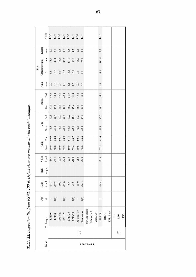
Tab
le 2
2. I
nspe
ctio
n li
st fr
om F
SWL
100
-6. D
efec
t siz
es a
re m
easu
red
wit
h ea
ch te
chni
que.
S
ize
Def
. S
ign
Sig
n N
oise
A
xial
C
irc
Rad
ial
Axi
al
Cir
cum
fere
ntia
l R
adia
l
Wel
d T
echn
ique
#
Am
pl
Ang
le
Am
pl
Sta
rt
End
Sta
rt
End
S
tart
E
nd
mm
°
mm
m
m
Not
es
FSWL 100-6
UT
LP
E 0
1
-18.
7
-30.
4 60
.0
60.0
71.5
80
.3
47.0
49
.0
0.0
8.8
73.4
2.
0 L
OP
LP
E 0
1(
2)
-17.
9
-32.
1 60
.0
60.0
46.9
57
.5
47.0
50
.0
0.0
10.6
88
.4
3.0
LO
P
LP
E +
20
1 -1
0.2
-2
3.0
59.9
60
.371
.0
80.0
45
.0
47.8
0.
4 9.
0 75
.4
2.8
LO
P
LP
E +
20
1(2)
-1
2.0
-2
4.0
59.9
60
.947
.0
57.2
46
.2
47.8
1.
0 10
.2
85.2
1.
6 L
OP
LP
E -
20
1 -5
.7
-2
3.0
59.9
61
.466
.8
80.2
48
.2
51.7
1.
5 13
.4
111.
5 3.
5 L
OP
LP
E -
20
1(2)
-1
.5
-2
0.0
59.4
60
.747
.0
57.8
47
.4
51.9
1.
3 10
.8
90.0
4.
5 L
OP
Roo
t sec
tor
1 -1
5.9
-2
5.0
60.6
60
.672
.1
80.0
46
.9
49.0
0.
0 7.
9 65
.9
2.1
LO
P
Roo
t sec
tor
1(2)
-1
4.5
-2
4.0
60.0
60
.047
.3
56.4
46
.9
50.0
0.
0 9.
1 75
.9
3.1
LO
P
Sur
face
sec
tor
Mat
sca
n A
Mat
sca
n C
TR
L-R
1
-14.
4
-25.
0 57
.5
61.6
56.9
80
.0
49.5
55
.2
4.1
23.1
19
1.4
5.7
LO
P
TR
L-C
TR
L_S
tart
ET
HF
LF
0
LF
90
63
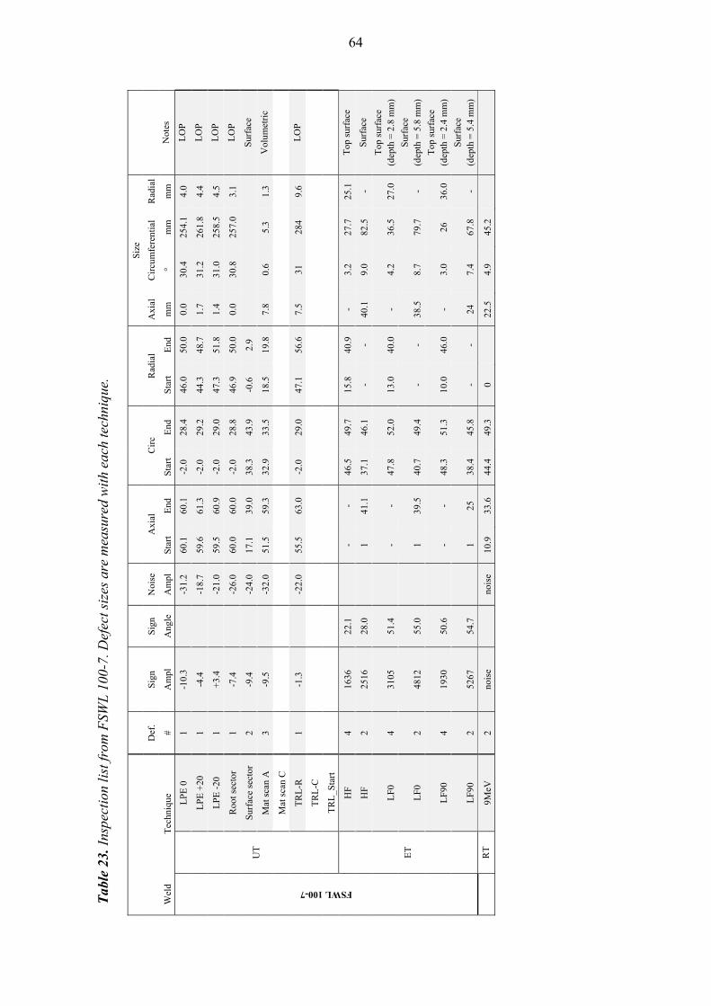
Tab
le 2
3. I
nspe
ctio
n li
st fr
om F
SWL
100
-7. D
efec
t siz
es a
re m
easu
red
wit
h ea
ch te
chni
que.
Siz
e
Def
. S
ign
Sig
n N
oise
A
xial
C
irc
Rad
ial
Axi
al
Cir
cum
fere
ntia
l R
adia
l
Wel
d T
echn
ique
#
Am
pl
Ang
le
Am
pl
Sta
rt
End
S
tart
E
nd
Sta
rt
End
m
m
° m
m
mm
N
otes
FSWL 100-7
UT
LP
E 0
1
-10.
3 -3
1.2
60.1
60
.1
-2.0
28
.4
46.0
50
.0
0.0
30.4
25
4.1
4.0
LO
P
LP
E +
20
1 -4
.4
-18.
7 59
.6
61.3
-2
.0
29.2
44
.3
48.7
1.
7 31
.2
261.
8 4.
4 L
OP
LP
E -
20
1 +
3.4
-21.
0 59
.5
60.9
-2
.0
29.0
47
.3
51.8
1.
4 31
.0
258.
5 4.
5 L
OP
Roo
t sec
tor
1 -7
.4
-26.
0 60
.0
60.0
-2
.0
28.8
46
.9
50.0
0.
0 30
.8
257.
0 3.
1 L
OP
Sur
face
sec
tor
2 -9
.4
-24.
0 17
.1
39.0
38
.3
43.9
-0
.6
2.9
Sur
face
Mat
sca
n A
3
-9.5
-3
2.0
51.5
59
.3
32.9
33
.5
18.5
19
.8
7.8
0.6
5.3
1.3
Vol
umet
ric
Mat
sca
n C
TR
L-R
1
-1.3
-2
2.0
55.5
63
.0
-2.0
29
.0
47.1
56
.6
7.5
31
284
9.6
LO
P
TR
L-C
TR
L_S
tart
ET
HF
4
1636
22
.1
- -
46.5
49
.7
15.8
40
.9
- 3.
2 27
.7
25.1
T
op s
urfa
ce
HF
2
2516
28
.0
1 41
.1
37.1
46
.1
- -
40.1
9.
0 82
.5
- S
urfa
ce
LF
0 4
3105
51
.4
- -
47.8
52
.0
13.0
40
.0
- 4.
2 36
.5
27.0
T
op s
urfa
ce
(dep
th =
2.8
mm
)
LF
0 2
4812
55
.0
1 39
.5
40.7
49
.4
- -
38.5
8.
7 79
.7
- S
urfa
ce
(dep
th =
5.8
mm
)
LF
90
4 19
30
50.6
-
- 48
.3
51.3
10
.0
46.0
-
3.0
26
36.0
T
op s
urfa
ce
(dep
th =
2.4
mm
)
LF
90
2 52
67
54.7
1
25
38.4
45
.8
- -
24
7.4
67.8
-
Sur
face
(d
epth
= 5
.4 m
m)
RT
9M
eV
2 no
ise
nois
e 10
.9
33.6
44
.4
49.3
0
22.5
4.
9 45
.2
64
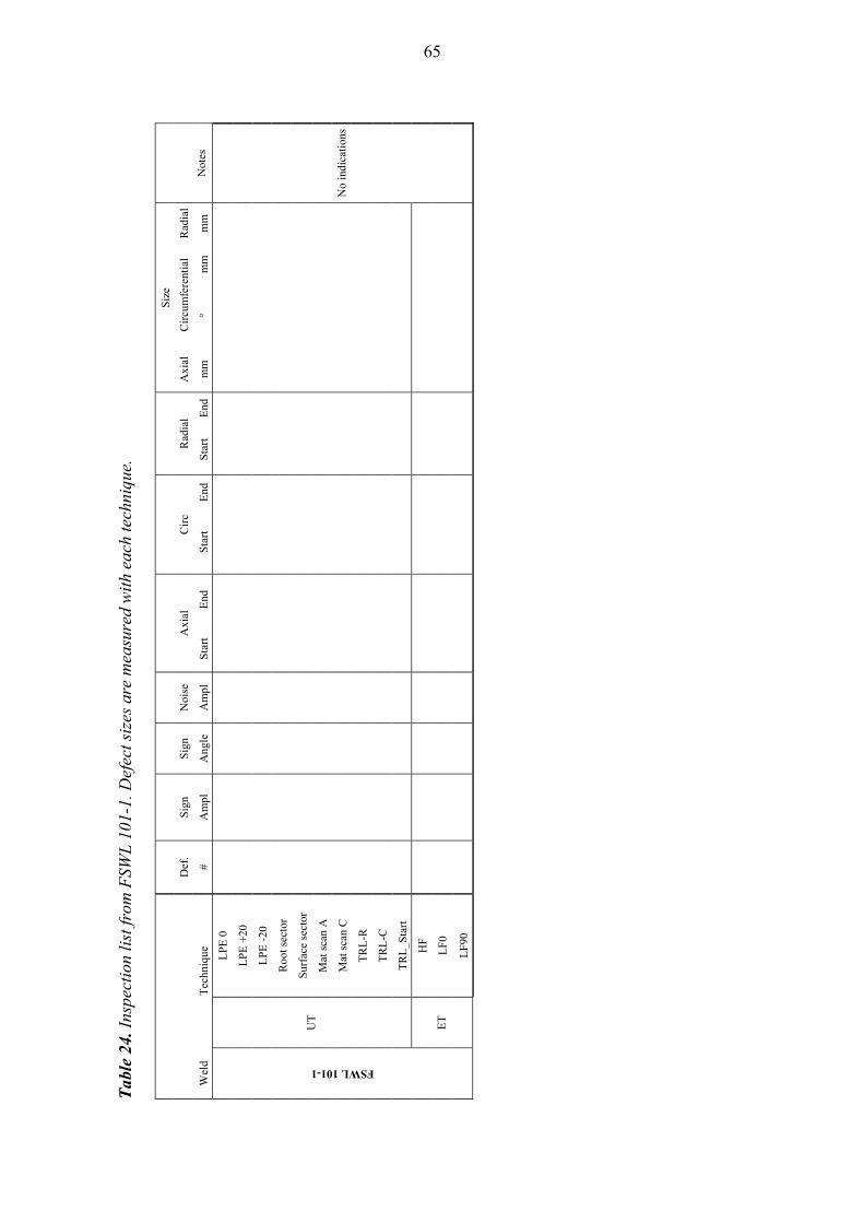
Tab
le 2
4. I
nspe
ctio
n li
st fr
om F
SWL
101
-1. D
efec
t siz
es a
re m
easu
red
wit
h ea
ch te
chni
que.
S
ize
Def
. S
ign
Sig
n N
oise
A
xial
C
irc
Rad
ial
Axi
al
Cir
cum
fere
ntia
l R
adia
l
Wel
d T
echn
ique
#
Am
pl
Ang
le
Am
pl
Sta
rt
End
S
tart
E
nd
Sta
rt
End
m
m
° m
m
mm
N
otes
FSWL 101-1
UT
LP
E 0
No
indi
cati
ons
LP
E +
20
LP
E -
20
Roo
t sec
tor
Sur
face
sec
tor
Mat
sca
n A
Mat
sca
n C
TR
L-R
TR
L-C
TR
L_S
tart
ET
HF
LF
0
LF
90
65
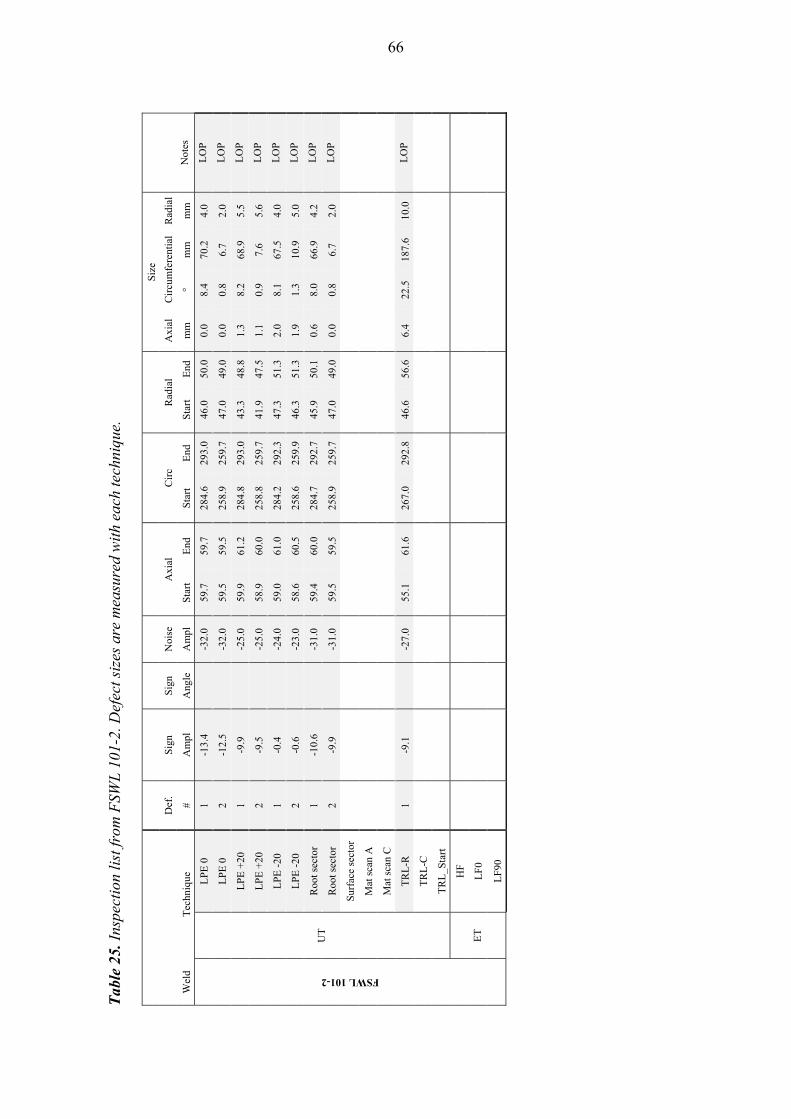
Tab
le 2
5. I
nspe
ctio
n li
st fr
om F
SWL
101
-2. D
efec
t siz
es a
re m
easu
red
wit
h ea
ch te
chni
que.
S
ize
Def
. S
ign
Sig
n N
oise
A
xial
C
irc
Rad
ial
Axi
al
Cir
cum
fere
ntia
l R
adia
l
Wel
d T
echn
ique
#
Am
pl
Ang
le
Am
pl
Sta
rt
End
S
tart
E
nd
Sta
rt
End
m
m
° m
m
mm
N
otes
FSWL 101-2
UT
LP
E 0
1
-13.
4
-32.
0 59
.7
59.7
28
4.6
293.
0 46
.0
50.0
0.
0 8.
4 70
.2
4.0
LO
P
LP
E 0
2
-12.
5
-32.
0 59
.5
59.5
25
8.9
259.
7 47
.0
49.0
0.
0 0.
8 6.
7 2.
0 L
OP
LP
E +
20
1 -9
.9
-2
5.0
59.9
61
.2
284.
8 29
3.0
43.3
48
.8
1.3
8.2
68.9
5.
5 L
OP
LP
E +
20
2 -9
.5
-2
5.0
58.9
60
.0
258.
8 25
9.7
41.9
47
.5
1.1
0.9
7.6
5.6
LO
P
LP
E -
20
1 -0
.4
-2
4.0
59.0
61
.0
284.
2 29
2.3
47.3
51
.3
2.0
8.1
67.5
4.
0 L
OP
LP
E -
20
2 -0
.6
-2
3.0
58.6
60
.5
258.
6 25
9.9
46.3
51
.3
1.9
1.3
10.9
5.
0 L
OP
Roo
t sec
tor
1 -1
0.6
-3
1.0
59.4
60
.0
284.
7 29
2.7
45.9
50
.1
0.6
8.0
66.9
4.
2 L
OP
Roo
t sec
tor
2 -9
.9
-3
1.0
59.5
59
.5
258.
9 25
9.7
47.0
49
.0
0.0
0.8
6.7
2.0
LO
P
Sur
face
sec
tor
Mat
sca
n A
Mat
sca
n C
TR
L-R
1
-9.1
-27.
0 55
.1
61.6
26
7.0
292.
8 46
.6
56.6
6.
4 22
.5
187.
6 10
.0
LO
P
TR
L-C
TR
L_S
tart
ET
HF
LF
0
LF
90
66

Tab
le 2
6. I
nspe
ctio
n li
st fr
om F
SWL
101
-3. D
efec
t siz
es a
re m
easu
red
wit
h ea
ch te
chni
que.
S
ize
Def
. S
ign
Sig
n N
oise
A
xial
C
irc
Rad
ial
Axi
al
Cir
cum
fere
ntia
l R
adia
l
Wel
d T
echn
ique
#
Am
pl
Ang
le
Am
pl
Sta
rt
End
S
tart
E
nd
Sta
rt
End
m
m
° m
m
mm
N
otes
FSWL 101-3
UT
LP
E 0
1
-7.8
-33.
0 59
.9
59.9
23
3.4
240.
2 45
.0
50.0
0.
0 6.
8 57
.0
5.0
LO
P
LP
E +
20
1 -3
.4
-2
1.0
59.4
60
.7
234.
0 24
0.0
44.1
47
.6
1.3
6.0
50.4
3.
5 L
OP
LP
E -
20
1 +
5.5
-2
2.0
59.0
60
.9
230.
8 24
0.8
46.5
50
.8
1.9
10.0
83
.5
4.3
LO
P
Roo
t sec
tor
1 -5
.4
-3
1.0
59.7
59
.7
233.
8 24
0.5
49.0
45
.9
0.0
6.7
55.7
-3
.1
LO
P
Sur
face
sec
tor
Mat
sca
n A
Mat
sca
n C
TR
L-R
1
0
-27.
0 54
.1
62.8
23
1.7
245.
2 44
.2
57.1
8.
7 13
.4
112.
6 12
.9
LO
P
TR
L-C
TR
L_S
tart
ET
HF
LF
0
LF
90
67
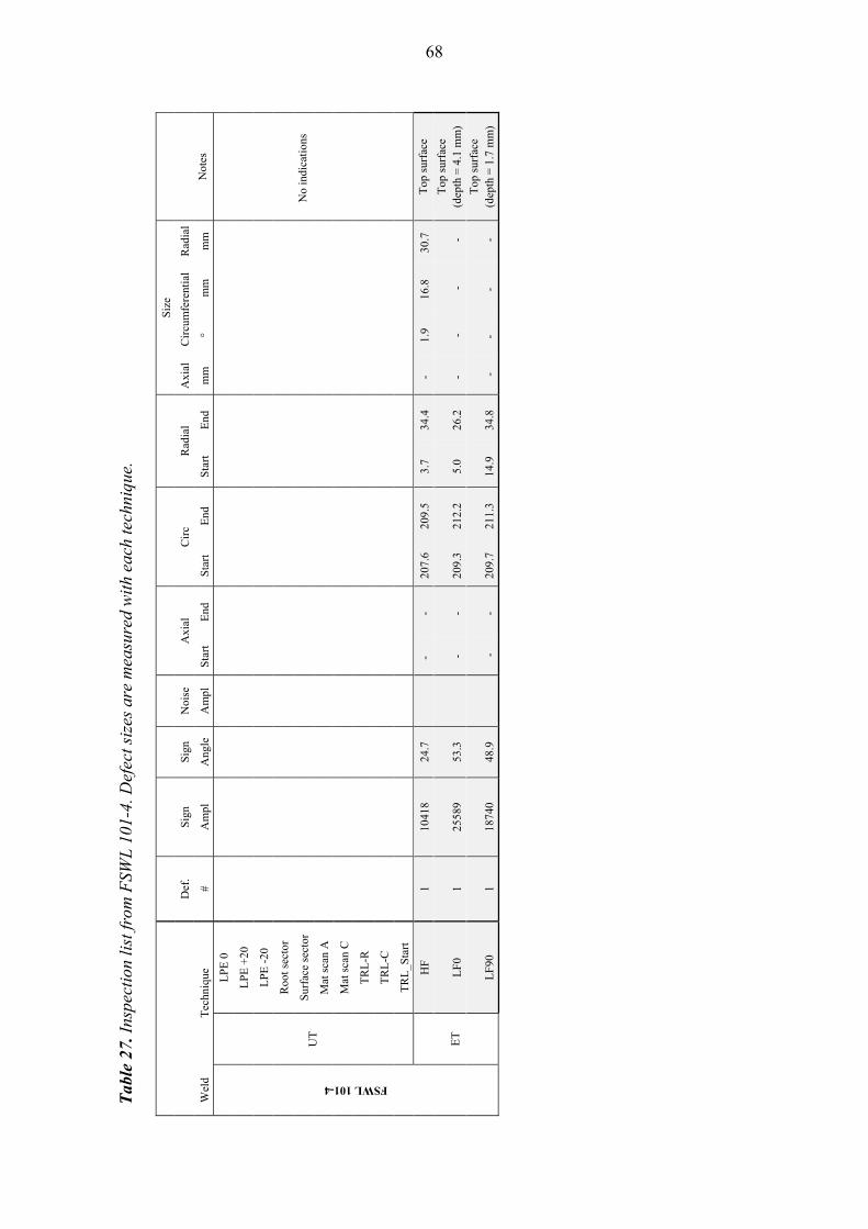
Tab
le 2
7. I
nspe
ctio
n li
st fr
om F
SWL
101
-4. D
efec
t siz
es a
re m
easu
red
wit
h ea
ch te
chni
que.
S
ize
Def
. S
ign
Sig
n N
oise
A
xial
C
irc
Rad
ial
Axi
al
Cir
cum
fere
ntia
l R
adia
l
Wel
d T
echn
ique
#
Am
pl
Ang
le
Am
pl
Sta
rt
End
S
tart
E
nd
Sta
rt
End
m
m
° m
m
mm
N
otes
FSWL 101-4
UT
LP
E 0
LP
E +
20
LP
E -
20
Roo
t sec
tor
Sur
face
sec
tor
N
o in
dica
tion
s
Mat
sca
n A
Mat
sca
n C
TR
L-R
TR
L-C
TR
L_S
tart
ET
HF
1
1041
8 24
.7
-
-
20
7.6
209.
5 3.
7 34
.4
-
1.9
16.8
30
.7
Top
sur
face
LF
0 1
2558
9 53
.3
-
-
209.
3 21
2.2
5.0
26.2
-
-
- -
T
op s
urfa
ce
(dep
th =
4.1
mm
)
LF
90
1 18
740
48.9
-
-
209.
7 21
1.3
14.9
34
.8
-
-
-
-
Top
sur
face
(d
epth
= 1
.7 m
m)
68
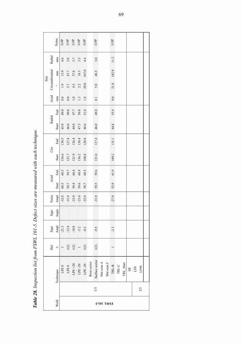
Tab
le 2
8. I
nspe
ctio
n li
st fr
om F
SWL
101
-5. D
efec
t siz
es a
re m
easu
red
wit
h ea
ch te
chni
que.
S
ize
Def
. S
ign
Sig
n N
oise
A
xial
C
irc
Rad
ial
Axi
al
Cir
cum
fere
ntia
l R
adia
l
Wel
d T
echn
ique
#
Am
pl
Ang
le
Am
pl
Sta
rt
End
S
tart
E
nd
Sta
rt
End
m
m
° m
m
mm
N
otes
FSWL 101-5
UT
LP
E 0
1
-21.
3
-32.
0 60
.5
60.5
13
6.6
138.
5 45
.0
49.0
0.
0 1.
9 15
.9
4.0
LO
P
LP
E 0
1(
2)
-12.
9
-31.
0 59
.7
59.7
12
1.7
127.
4 46
.0
49.0
0.
0 5.
7 47
.7
3.0
LO
P
LP
E +
20
1(2)
-1
0.8
-2
3.0
59.4
60
.4
121.
9 12
6.4
44.0
47
.7
1.0
4.5
37.8
3.
7 L
OP
LP
E -
20
1 -5
.2
-2
3.0
59.6
60
.9
136.
2 13
8.4
47.3
50
.8
1.3
2.2
18.3
3.
5 L
OP
LP
E -
20
1(2)
-0
.2
-2
2.0
58.7
60
.5
108.
8 12
8.8
46.6
51
.0
1.8
20.0
16
7.0
4.4
LO
P
Roo
t sec
tor
Sur
face
sec
tor
1(2)
-9
.5
-3
1.0
59.5
59
.6
121.
6 12
7.4
46.0
49
.0
0.1
5.8
48.5
3.
0 L
OP
Mat
sca
n A
Mat
sca
n C
TR
L-R
1
-2.3
-27.
0 52
.9
61.9
10
9.2
131.
1 44
.8
55.9
9.
0 21
.8
182.
9 11
.2
LO
P
TR
L-C
TR
L_S
tart
HF
ET
LF
0
LF
90
69
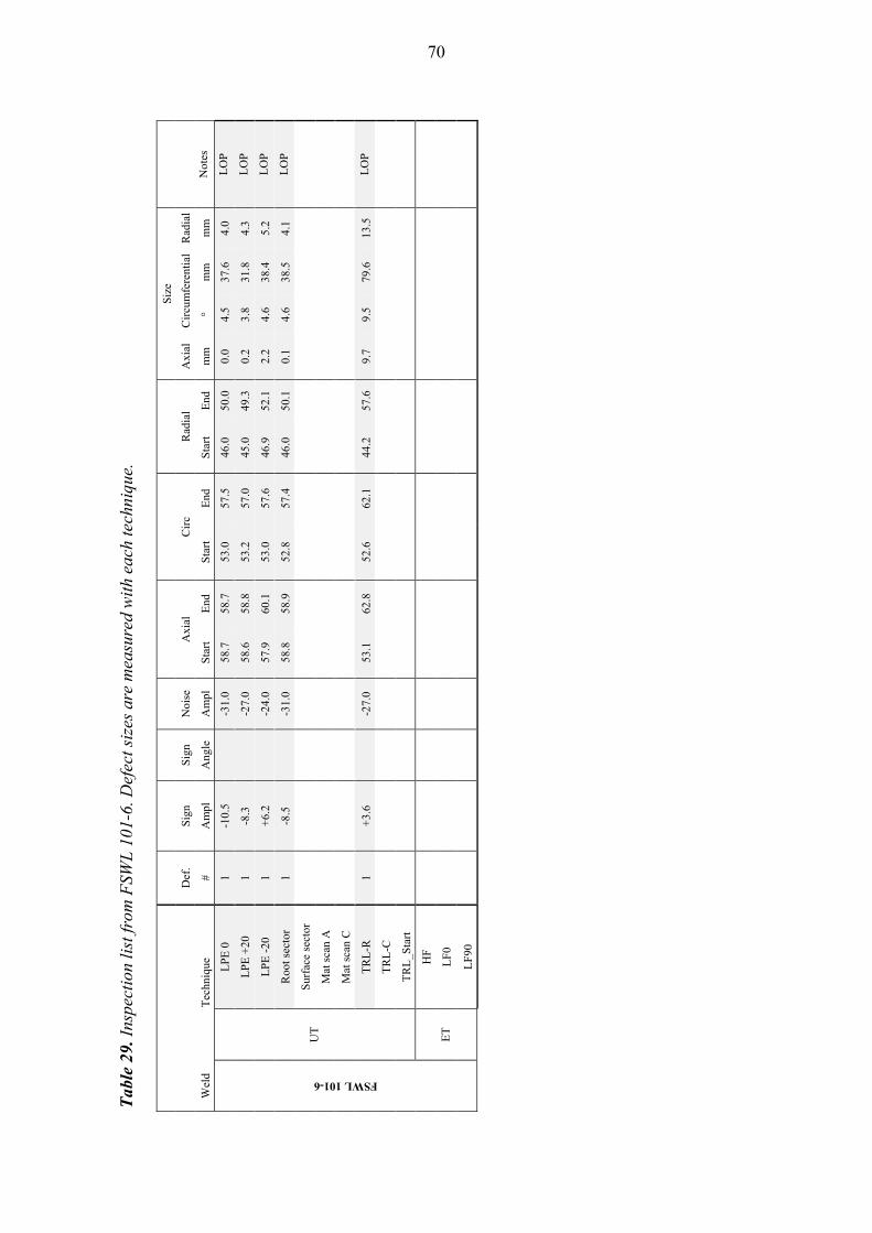
Tab
le 2
9. I
nspe
ctio
n li
st fr
om F
SWL
101
-6. D
efec
t siz
es a
re m
easu
red
wit
h ea
ch te
chni
que.
S
ize
Def
. S
ign
Sig
n N
oise
A
xial
C
irc
Rad
ial
Axi
al
Cir
cum
fere
ntia
lR
adia
l
Wel
d T
echn
ique
#
Am
pl
Ang
le
Am
pl
Sta
rt
End
S
tart
E
nd
Sta
rt
End
m
m
° m
m
mm
N
otes
FSWL 101-6
UT
LP
E 0
1
-10.
5
-31.
0 58
.7
58.7
53
.0
57.5
46
.0
50.0
0.
0 4.
5 37
.6
4.0
LO
P
LP
E +
20
1 -8
.3
-2
7.0
58.6
58
.8
53.2
57
.0
45.0
49
.3
0.2
3.8
31.8
4.
3 L
OP
LP
E -
20
1 +
6.2
-2
4.0
57.9
60
.1
53.0
57
.6
46.9
52
.1
2.2
4.6
38.4
5.
2 L
OP
Roo
t sec
tor
1 -8
.5
-3
1.0
58.8
58
.9
52.8
57
.4
46.0
50
.1
0.1
4.6
38.5
4.
1 L
OP
Sur
face
sec
tor
Mat
sca
n A
Mat
sca
n C
TR
L-R
1
+3.
6
-27.
0 53
.1
62.8
52
.6
62.1
44
.2
57.6
9.
7 9.
5 79
.6
13.5
L
OP
TR
L-C
TR
L_S
tart
ET
HF
LF
0
LF
90
70
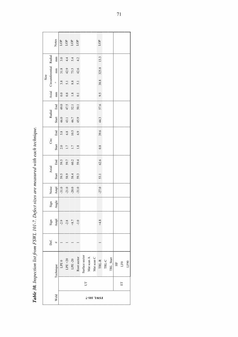
Tab
le 3
0. I
nspe
ctio
n li
st fr
om F
SWL
101
-7. D
efec
t siz
es a
re m
easu
red
wit
h ea
ch te
chni
que.
S
ize
Def
. S
ign
Sig
n N
oise
A
xial
C
irc
Rad
ial
Axi
al
Cir
cum
fere
ntia
lR
adia
l
Wel
d T
echn
ique
#
Am
pl
Ang
le
Am
pl
Sta
rt
End
S
tart
E
nd
Sta
rt
End
m
m
° m
m
mm
N
otes
FSWL 101-7
UT
LP
E 0
1
-2.9
-31.
0 59
.5
59.5
2.
0 5.
8 46
.0
49.0
0.
0 3.
8 31
.8
3.0
LO
P
LP
E +
20
1 -2
.8
-2
1.0
58.9
59
.7
1.7
6.8
43.1
47
.5
0.8
5.1
42.9
4.
4 L
OP
LP
E -
20
1 +
8.7
-2
0.0
58.4
60
.2
1.7
10.5
46
.7
52.1
1.
8 8.
8 73
.5
5.4
LO
P
Roo
t sec
tor
1 -1
.0
-3
1.0
59.3
59
.4
1.8
6.9
45.9
50
.1
0.1
5.1
42.6
4.
2 L
OP
Sur
face
sec
tor
Mat
sca
n A
Mat
sca
n C
TR
L-R
1
+4.
8
-27.
0 53
.1
62.6
0.
8 39
.6
44.3
57
.6
9.5
38.8
32
5.8
13.3
L
OP
TR
L-C
TR
L_S
tart
ET
HF
LF
0
LF
90
71
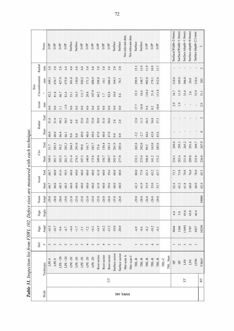
Tab
le 3
1. I
nspe
ctio
n li
st fr
om F
SWL
102
. Def
ect s
izes
are
mea
sure
d w
ith
each
tech
niqu
e.
S
ize
Def
. S
ign
Sig
n N
oise
A
xial
C
irc
Rad
ial
Axi
al
Cir
cum
fere
ntia
l R
adia
l
Wel
d T
echn
ique
#
Am
pl
Ang
le
Am
pl
Sta
rt
End
S
tart
E
nd
Sta
rt
End
m
m
° m
m
mm
N
otes
FSWL 102
UT
LP
E 0
3
-16.
5
-29.
0 60
.7
60.7
34
9.5
31.7
48
.0
51.0
0.
0 42
.2
349.
1 3.
0 L
OP
LP
E 0
5
-10.
7
-28.
0 60
.0
60.0
20
1.7
283.
5 48
.0
51.0
0.
0 81
.8
676.
7 3.
0 L
OP
LP
E +
20
3 -9
.6
-2
0.0
60.5
61
.6
343.
5 30
.2
46.4
49
.2
1.1
46.7
42
7.9
2.8
LO
P
LP
E +
20
5 -6
.7
-1
9.0
60.5
59
.5
201.
7 28
3.3
46.1
50
.5
-1.0
81
.6
675.
8 4.
4 L
OP
LP
E -
20
1 +
4.4
-2
1.0
68.0
68
.0
231.
4 26
4.5
0.0
4.0
0.0
33.1
30
1.0
4.0
Sur
face
LP
E -
20
2 +
1.7
-2
3.0
69.0
69
.0
274.
5 29
1.0
0.0
4.0
0.0
16.5
15
0.0
4.0
Sur
face
LP
E -
20
3 -3
.1
-2
3.0
60.0
60
.0
347.
3 99
.0
49.0
53
.0
0.0
111.
7 92
0.2
4.0
LO
P
LP
E -
20
4 -7
.2
-2
3.0
60.0
60
.0
140.
9 16
1.7
48.0
53
.0
0.0
20.8
17
1.3
5.0
LO
P
LP
E -
20
5 +
6.3
-2
3.0
60.0
60
.0
175.
8 28
3.7
49.0
53
.0
0.0
107.
9 88
8.9
4.0
LO
P
Roo
t sec
tor
3 -1
4.5
-2
5.0
61.0
61
.0
349.
4 55
.6
47.0
50
.0
0.0
66.2
54
8.8
3.0
LO
P
Roo
t sec
tor
4 -1
6.2
-2
6.0
60.0
60
.0
156.
7 15
8.4
48.0
51
.0
0.0
1.7
14.1
3.
0 L
OP
Roo
t sec
tor
5 -1
2.2
-2
6.0
59.6
59
.6
200.
7 28
3.5
47.0
50
.0
0.0
82.8
68
6.4
3.0
LO
P
Sur
face
sec
tor
1 -1
9.0
-2
5.0
68.0
68
.0
243.
9 26
1.9
0.0
2.0
0.0
18.0
16
4.3
2.0
Sur
face
Sur
face
sec
tor
2 -2
0.0
-2
6.0
68.0
68
.0
277.
0 28
5.6
0.0
2.0
0.0
8.6
78.5
2.
0 S
urfa
ce
Mat
sca
n A
N
ot r
elev
ant d
ata
Mat
sca
n C
N
ot r
elev
ant d
ata
TR
L-R
1
-6.9
-29.
0 62
.3
80.0
23
2.3
265.
8 -3
.2
12.0
17
.7
33.5
29
9.9
15.2
S
urfa
ce
TR
L-R
2
-8.6
-28.
0 61
.9
77.9
27
5.4
292.
0 -2
.7
11.3
16
.0
16.6
14
8.7
13.9
S
urfa
ce
TR
L-R
3
-8.2
-26.
0 53
.9
63.3
34
8.8
99.2
44
.6
56.5
9.
4 11
0.4
902.
8 11
.9
LO
P
TR
L-R
4
-10.
2
-28.
0 55
.0
63.2
14
1.2
163.
0 43
.9
54.8
8.
2 21
.8
179.
1 10
.9
LO
P
TR
L-R
5
-0.3
-29.
0 53
.7
63.7
17
3.2
285.
0 43
.6
57.3
10
.0
111.
8 91
2.8
13.7
L
OP
TR
L-C
TR
L_S
tart
ET
HF
1
9044
6.
4
62.4
73
.3
234.
3 26
9.0
- -
2.9
34
.7
318.
0 -
Sur
face
(Wid
th=
2.9m
m)
HF
2
1360
5.
8
65.2
73
.8
283.
4 29
5.3
- -
1
.9
11.9
10
9.0
-
Sur
face
(Wid
th=
1.9m
m)
LF
0 1
1189
3 45
.0
61
.8
79.8
23
1.8
265.
2 -
-
-
33.4
30
6.0
-
Sur
face
(de
pth=
1.9m
m)
LF
0 2
3787
45
.0
68
.0
76,0
28
9.0
291.
6 -
-
-
2.6
24.0
-
S
urfa
ce (
dept
h=0.
8mm
)
LF
90
1 69
27
46.4
60.0
78
.0
235.
8 26
9.7
-
-
-
33.9
31
0.6
-
Surf
ace
(dep
th=2
.3 m
m)
RT
9
MeV
10
250
1000
0 62
.4
65.3
23
6.8
267.
9 0
2 2.
9 31
.1
285
2 2
72
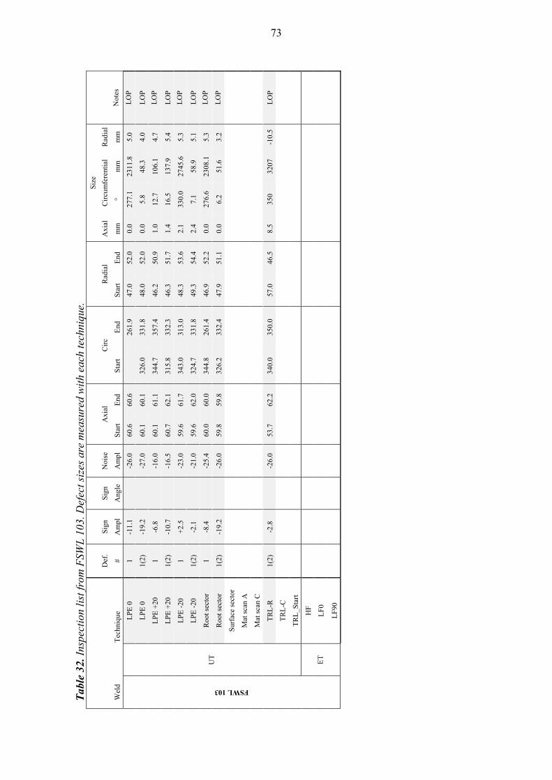
Tab
le 3
2. I
nspe
ctio
n li
st fr
om F
SWL
103
. Def
ect s
izes
are
mea
sure
d w
ith
each
tech
niqu
e.
S
ize
Def
. S
ign
Sig
n N
oise
A
xial
C
irc
Rad
ial
Axi
al
Cir
cum
fere
ntia
l R
adia
l
Wel
d T
echn
ique
#
Am
pl
Ang
le
Am
pl
Sta
rt
End
S
tart
E
nd
Sta
rt
End
m
m
° m
m
mm
N
otes
FSWL 103
UT
LP
E 0
1
-11.
1
-26.
0 60
.6
60.6
261.
9 47
.0
52.0
0.
0 27
7.1
2311
.8
5.0
LO
P
LP
E 0
1(
2)
-19.
2
-27.
0 60
.1
60.1
32
6.0
331.
8 48
.0
52.0
0.
0 5.
8 48
.3
4.0
LO
P
LP
E +
20
1 -6
.8
-1
6.0
60.1
61
.1
344.
7 35
7.4
46.2
50
.9
1.0
12.7
10
6.1
4.7
LO
P
LP
E +
20
1(2)
-1
0.7
-1
6.5
60.7
62
.1
315.
8 33
2.3
46.3
51
.7
1.4
16.5
13
7.9
5.4
LO
P
LP
E -
20
1 +
2.5
-2
3.0
59.6
61
.7
343.
0 31
3.0
48.3
53
.6
2.1
330.
0 27
45.6
5.
3 L
OP
LP
E -
20
1(2)
-2
.1
-2
1.0
59.6
62
.0
324.
7 33
1.8
49.3
54
.4
2.4
7.1
58.9
5.
1 L
OP
Roo
t sec
tor
1 -8
.4
-2
5.4
60.0
60
.0
344.
8 26
1.4
46.9
52
.2
0.0
276.
6 23
08.1
5.
3 L
OP
Roo
t sec
tor
1(2)
-1
9.2
-2
6.0
59.8
59
.8
326.
2 33
2.4
47.9
51
.1
0.0
6.2
51.6
3.
2 L
OP
Sur
face
sec
tor
Mat
sca
n A
Mat
sca
n C
TR
L-R
1(
2)
-2.8
-26.
0 53
.7
62.2
34
0.0
350.
0 57
.0
46.5
8.
5 35
0 32
07
-10.
5 L
OP
TR
L-C
TR
L_S
tart
ET
HF
LF
0
LF
90
73

74
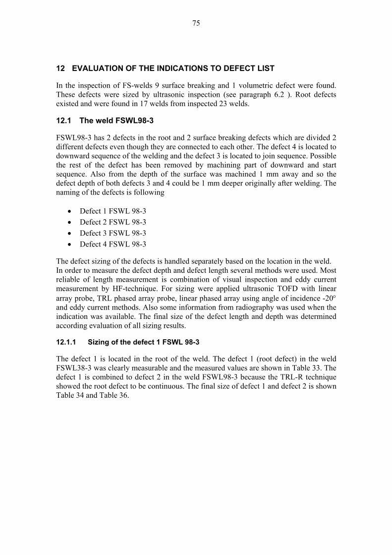
75
12 EVALUATION OF THE INDICATIONS TO DEFECT LIST
In the inspection of FS-welds 9 surface breaking and 1 volumetric defect were found. These defects were sized by ultrasonic inspection (see paragraph 6.2 ). Root defects existed and were found in 17 welds from inspected 23 welds.
12.1 The weld FSWL98-3
FSWL98-3 has 2 defects in the root and 2 surface breaking defects which are divided 2 different defects even though they are connected to each other. The defect 4 is located to downward sequence of the welding and the defect 3 is located to join sequence. Possible the rest of the defect has been removed by machining part of downward and start sequence. Also from the depth of the surface was machined 1 mm away and so the defect depth of both defects 3 and 4 could be 1 mm deeper originally after welding. The naming of the defects is following
Defect 1 FSWL 98-3
Defect 2 FSWL 98-3
Defect 3 FSWL 98-3
Defect 4 FSWL 98-3
The defect sizing of the defects is handled separately based on the location in the weld. In order to measure the defect depth and defect length several methods were used. Most reliable of length measurement is combination of visual inspection and eddy current measurement by HF-technique. For sizing were applied ultrasonic TOFD with linear array probe, TRL phased array probe, linear phased array using angle of incidence -20 and eddy current methods. Also some information from radiography was used when the indication was available. The final size of the defect length and depth was determined according evaluation of all sizing results.
12.1.1 Sizing of the defect 1 FSWL 98-3
The defect 1 is located in the root of the weld. The defect 1 (root defect) in the weld FSWL38-3 was clearly measurable and the measured values are shown in Table 33. The defect 1 is combined to defect 2 in the weld FSWL98-3 because the TRL-R technique showed the root defect to be continuous. The final size of defect 1 and defect 2 is shown Table 34 and Table 36.
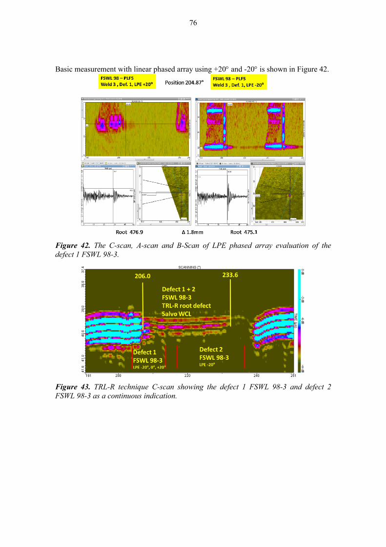
76
Basic measurement with linear phased array using +20 and -20 is shown in Figure 42.
Figure 42. The C-scan, A-scan and B-Scan of LPE phased array evaluation of the defect 1 FSWL 98-3.
Figure 43. TRL-R technique C-scan showing the defect 1 FSWL 98-3 and defect 2 FSWL 98-3 as a continuous indication.
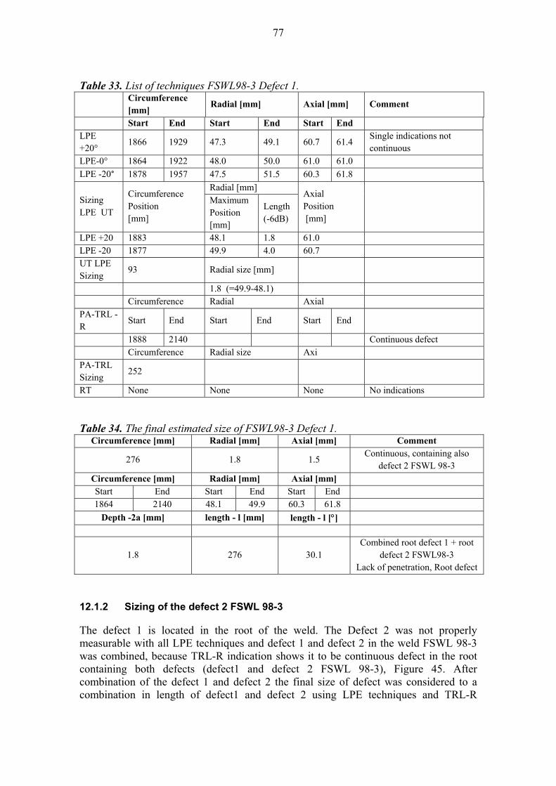
77
Table 33. List of techniques FSWL98-3 Defect 1.
Circumference [mm]
Radial [mm] Axial [mm] Comment
Start End Start End Start End LPE +20°
1866 1929 47.3 49.1 60.7 61.4 Single indications not continuous
LPE-0° 1864 1922 48.0 50.0 61.0 61.0
LPE -20° 1878 1957 47.5 51.5 60.3 61.8
Sizing LPE UT
Circumference Position [mm]
Radial [mm] Axial Position [mm]
Maximum Position [mm]
Length (-6dB)
LPE +20 1883 48.1 1.8 61.0 LPE -20 1877 49.9 4.0 60.7 UT LPE Sizing
93 Radial size [mm]
1.8 (=49.9-48.1) Circumference Radial Axial PA-TRL -R
Start End Start End Start End
1888 2140 Continuous defect Circumference Radial size Axi PA-TRL Sizing
252
RT None None None No indications
Table 34. The final estimated size of FSWL98-3 Defect 1. Circumference [mm] Radial [mm] Axial [mm] Comment
276 1.8 1.5 Continuous, containing also
defect 2 FSWL 98-3
Circumference [mm] Radial [mm] Axial [mm]
Start End Start End Start End
1864 2140 48.1 49.9 60.3 61.8
Depth -2a [mm] length - l [mm] length - l []
1.8 276 30.1 Combined root defect 1 + root
defect 2 FSWL98-3 Lack of penetration, Root defect
12.1.2 Sizing of the defect 2 FSWL 98-3
The defect 1 is located in the root of the weld. The Defect 2 was not properly measurable with all LPE techniques and defect 1 and defect 2 in the weld FSWL 98-3 was combined, because TRL-R indication shows it to be continuous defect in the root containing both defects (defect1 and defect 2 FSWL 98-3), Figure 45. After combination of the defect 1 and defect 2 the final size of defect was considered to a combination in length of defect1 and defect 2 using LPE techniques and TRL-R
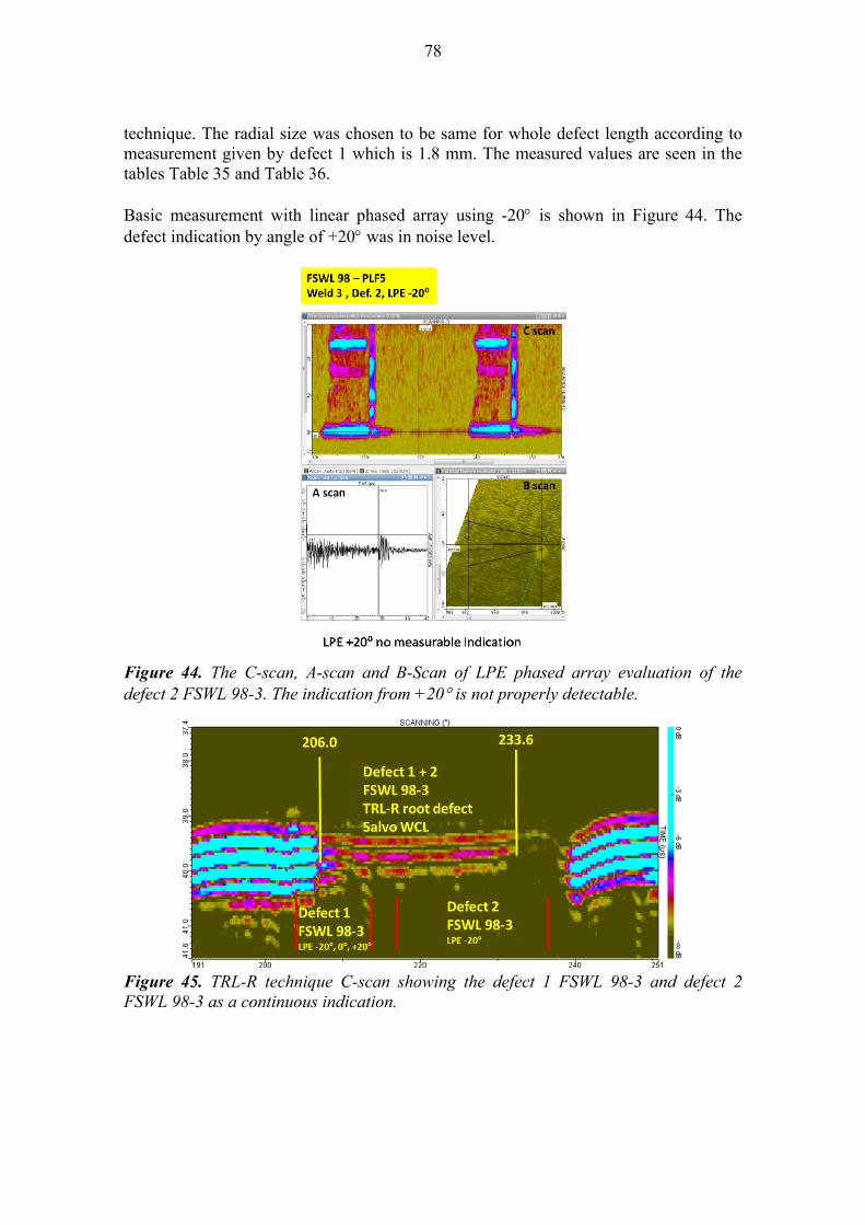
78
technique. The radial size was chosen to be same for whole defect length according to measurement given by defect 1 which is 1.8 mm. The measured values are seen in the tables Table 35 and Table 36. Basic measurement with linear phased array using -20 is shown in Figure 44. The defect indication by angle of +20 was in noise level.
Figure 44. The C-scan, A-scan and B-Scan of LPE phased array evaluation of the defect 2 FSWL 98-3. The indication from +20 is not properly detectable.
Figure 45. TRL-R technique C-scan showing the defect 1 FSWL 98-3 and defect 2 FSWL 98-3 as a continuous indication.
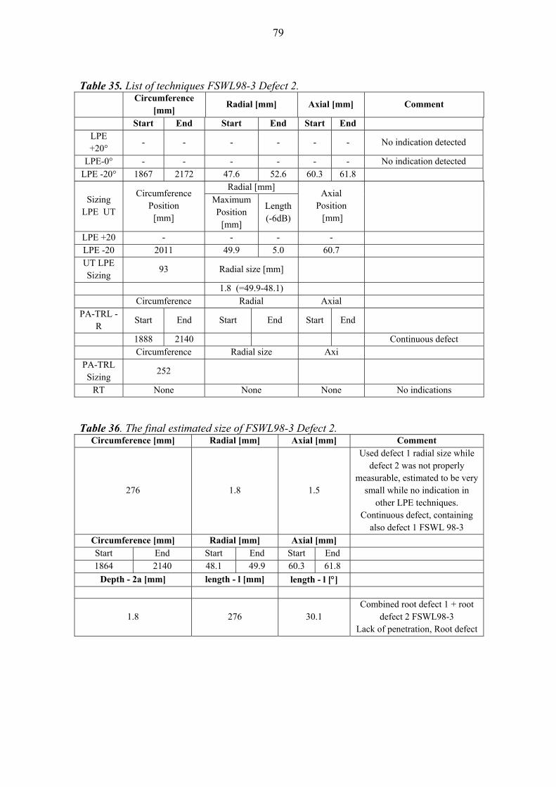
79
Table 35. List of techniques FSWL98-3 Defect 2.
Circumference
[mm] Radial [mm] Axial [mm] Comment
Start End Start End Start End LPE +20°
- - - - - - No indication detected
LPE-0° - - - - - - No indication detected LPE -20° 1867 2172 47.6 52.6 60.3 61.8
Sizing LPE UT
Circumference Position
[mm]
Radial [mm] Axial
Position [mm]
Maximum Position
[mm]
Length (-6dB)
LPE +20 - - - - LPE -20 2011 49.9 5.0 60.7 UT LPE Sizing
93 Radial size [mm]
1.8 (=49.9-48.1) Circumference Radial Axial
PA-TRL -R
Start End Start End Start End
1888 2140 Continuous defect Circumference Radial size Axi
PA-TRL Sizing
252
RT None None None No indications
Table 36. The final estimated size of FSWL98-3 Defect 2. Circumference [mm] Radial [mm] Axial [mm] Comment
276 1.8 1.5
Used defect 1 radial size while defect 2 was not properly
measurable, estimated to be very small while no indication in
other LPE techniques. Continuous defect, containing
also defect 1 FSWL 98-3 Circumference [mm] Radial [mm] Axial [mm]
Start End Start End Start End
1864 2140 48.1 49.9 60.3 61.8
Depth - 2a [mm] length - l [mm] length - l []
1.8 276 30.1 Combined root defect 1 + root
defect 2 FSWL98-3 Lack of penetration, Root defect
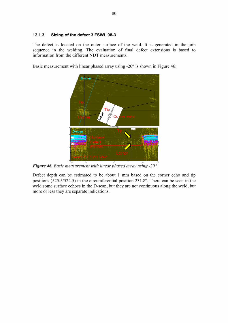
80
12.1.3 Sizing of the defect 3 FSWL 98-3
The defect is located on the outer surface of the weld. It is generated in the join sequence in the welding. The evaluation of final defect extensions is based to information from the different NDT measurements. Basic measurement with linear phased array using -20 is shown in Figure 46:
Figure 46. Basic measurement with linear phased array using -20.
Defect depth can be estimated to be about 1 mm based on the corner echo and tip positions (525.5/524.5) in the circumferential position 231.8. There can be seen in the weld some surface echoes in the D-scan, but they are not continuous along the weld, but more or less they are separate indications.

81
The TOFD measurement was performed for the defect3 FSWL 98-3. The sizing results are presented in Figure 47.
Figure 47. TOFD measurement of defect 3, FSWL 98-3.
TODF measurement gave 1 mm depth for the defect 3 FSWL 98-3. The circumferential position for depth sizing measurement was 237. The TOFD measurement showed the indication was continuous and the circumferential position was between 205.6 and 237.9 So the circumferential length of the defect was 296 mm (32.3) by TOFD technique. The probe centre axial position was 70 mm in the TOFD measurements. TRL70 measurement was performed for the defect 3 FSWL 98-3. The sizing results are presented in Figure 48.
Figure 48. The sizing results of TRL-70 matrix phased array probe of defect 3 FSWL 98-3.
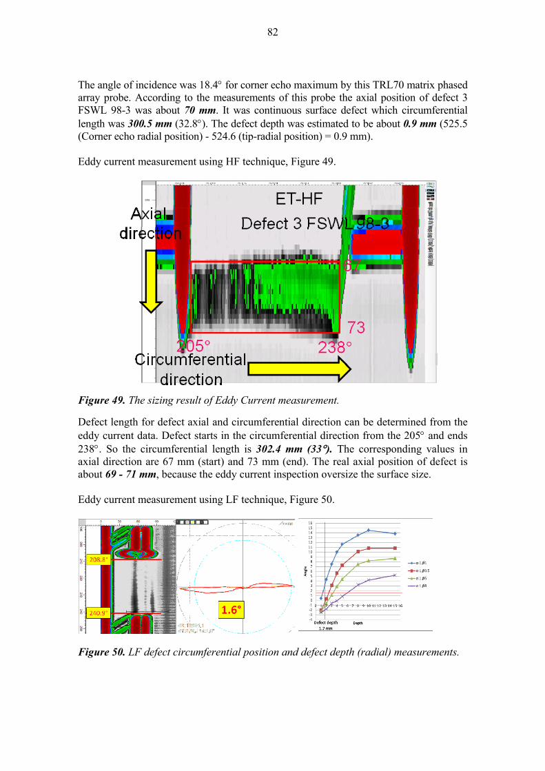
82
The angle of incidence was 18.4 for corner echo maximum by this TRL70 matrix phased array probe. According to the measurements of this probe the axial position of defect 3 FSWL 98-3 was about 70 mm. It was continuous surface defect which circumferential length was 300.5 mm (32.8). The defect depth was estimated to be about 0.9 mm (525.5 (Corner echo radial position) - 524.6 (tip-radial position) = 0.9 mm). Eddy current measurement using HF technique, Figure 49.
Figure 49. The sizing result of Eddy Current measurement.
Defect length for defect axial and circumferential direction can be determined from the eddy current data. Defect starts in the circumferential direction from the 205 and ends 238. So the circumferential length is 302.4 mm (33). The corresponding values in axial direction are 67 mm (start) and 73 mm (end). The real axial position of defect is about 69 - 71 mm, because the eddy current inspection oversize the surface size. Eddy current measurement using LF technique, Figure 50.
Figure 50. LF defect circumferential position and defect depth (radial) measurements.
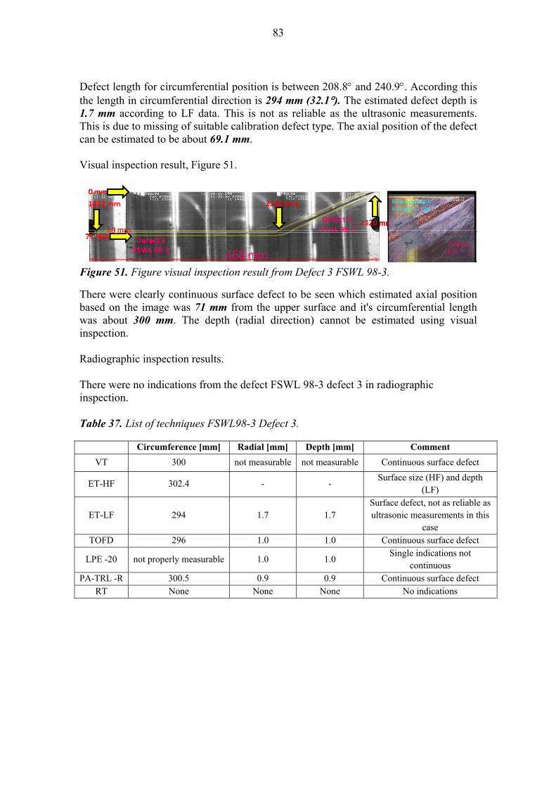
83
Defect length for circumferential position is between 208.8 and 240.9. According this the length in circumferential direction is 294 mm (32.1). The estimated defect depth is 1.7 mm according to LF data. This is not as reliable as the ultrasonic measurements. This is due to missing of suitable calibration defect type. The axial position of the defect can be estimated to be about 69.1 mm. Visual inspection result, Figure 51.
Figure 51. Figure visual inspection result from Defect 3 FSWL 98-3.
There were clearly continuous surface defect to be seen which estimated axial position based on the image was 71 mm from the upper surface and it's circumferential length was about 300 mm. The depth (radial direction) cannot be estimated using visual inspection. Radiographic inspection results. There were no indications from the defect FSWL 98-3 defect 3 in radiographic inspection. Table 37. List of techniques FSWL98-3 Defect 3.
Circumference [mm] Radial [mm] Depth [mm] Comment
VT 300 not measurable not measurable Continuous surface defect
ET-HF 302.4 - - Surface size (HF) and depth
(LF)
ET-LF 294 1.7 1.7 Surface defect, not as reliable as ultrasonic measurements in this
case TOFD 296 1.0 1.0 Continuous surface defect
LPE -20 not properly measurable 1.0 1.0 Single indications not
continuous PA-TRL -R 300.5 0.9 0.9 Continuous surface defect
RT None None None No indications
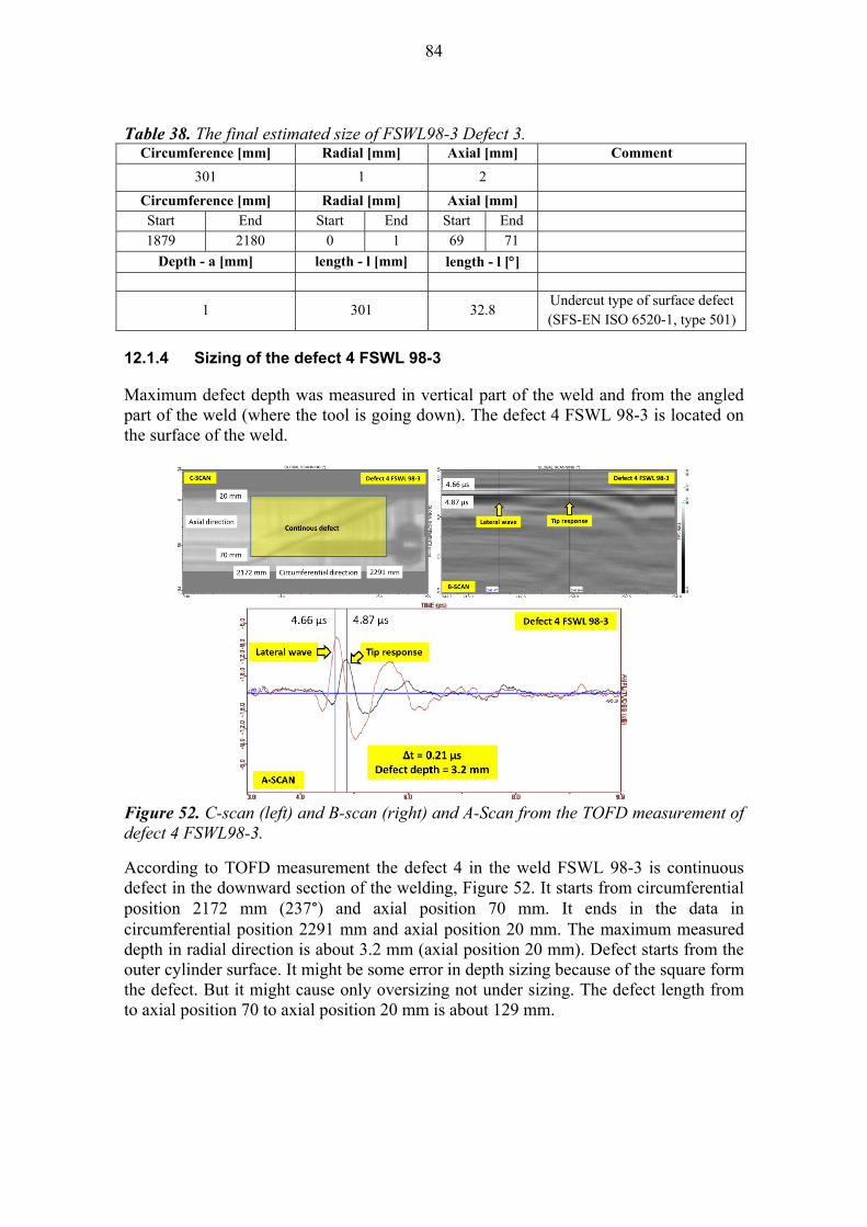
84
Table 38. The final estimated size of FSWL98-3 Defect 3. Circumference [mm] Radial [mm] Axial [mm] Comment
301 1 2
Circumference [mm] Radial [mm] Axial [mm]
Start End Start End Start End
1879 2180 0 1 69 71
Depth - a [mm] length - l [mm] length - l []
1 301 32.8 Undercut type of surface defect (SFS-EN ISO 6520-1, type 501)
12.1.4 Sizing of the defect 4 FSWL 98-3
Maximum defect depth was measured in vertical part of the weld and from the angled part of the weld (where the tool is going down). The defect 4 FSWL 98-3 is located on the surface of the weld.
Figure 52. C-scan (left) and B-scan (right) and A-Scan from the TOFD measurement of defect 4 FSWL98-3.
According to TOFD measurement the defect 4 in the weld FSWL 98-3 is continuous defect in the downward section of the welding, Figure 52. It starts from circumferential position 2172 mm (237°) and axial position 70 mm. It ends in the data in circumferential position 2291 mm and axial position 20 mm. The maximum measured depth in radial direction is about 3.2 mm (axial position 20 mm). Defect starts from the outer cylinder surface. It might be some error in depth sizing because of the square form the defect. But it might cause only oversizing not under sizing. The defect length from to axial position 70 to axial position 20 mm is about 129 mm.
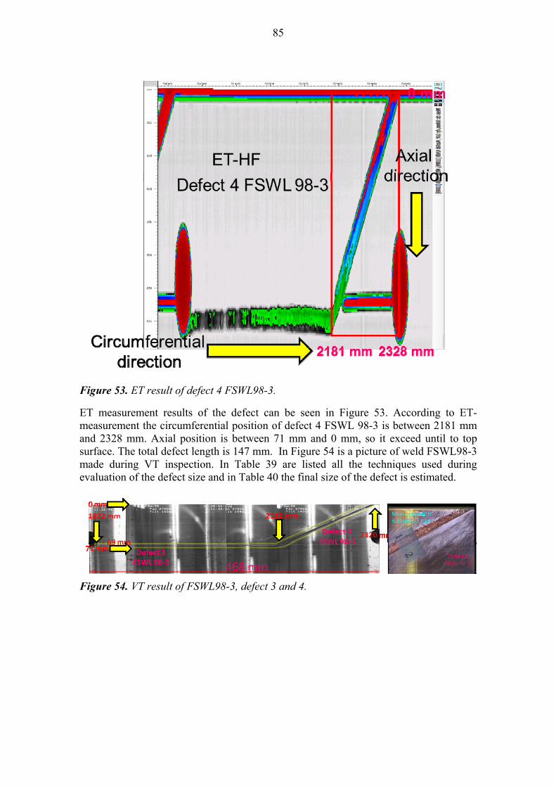
85
Figure 53. ET result of defect 4 FSWL98-3.
ET measurement results of the defect can be seen in Figure 53. According to ET-measurement the circumferential position of defect 4 FSWL 98-3 is between 2181 mm and 2328 mm. Axial position is between 71 mm and 0 mm, so it exceed until to top surface. The total defect length is 147 mm. In Figure 54 is a picture of weld FSWL98-3 made during VT inspection. In Table 39 are listed all the techniques used during evaluation of the defect size and in Table 40 the final size of the defect is estimated.
Figure 54. VT result of FSWL98-3, defect 3 and 4.
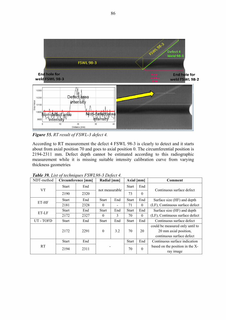
86
Figure 55. RT result of FSWL-3 defect 4.
According to RT measurement the defect 4 FSWL 98-3 is clearly to detect and it starts about from axial position 70 and goes to axial position 0. The circumferential position is 2194-2311 mm. Defect depth cannot be estimated according to this radiographic measurement while it is missing suitable intensity calibration curve from varying thickness geometries Table 39. List of techniques FSWL98-3 Defect 4. NDT-method Circumference [mm] Radial [mm] Axial [mm] Comment
VT Start End
not measurable Start End
Continuous surface defect 2190 2320 73 0
ET-HF Start End Start End Start End Surface size (HF) and depth
(LF), Continuous surface defect 2181 2328 0 - 71 0
ET-LF Start End Start End Start End Surface size (HF) and depth
(LF), Continuous surface defect 2172 2327 0 3 70 0 UT - TOFD Start End Start End Start End Continuous surface defect
2172 2291 0 3.2 70 20 could be measured only until to
20 mm axial position, continuous surface defect
RT Start End
- Start End Continuous surface indication
based on the position in the X-ray image
2194 2311 70 0
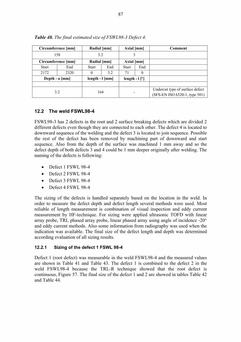
87
Table 40. The final estimated size of FSWL98-3 Defect 4.
Circumference [mm] Radial [mm] Axial [mm] Comment
158 3.2 3
Circumference [mm] Radial [mm] Axial [mm]
Start End Start End Start End
2172 2320 0 3.2 71 0
Depth - a [mm] length - l [mm] length - l []
3.2 164 - Undercut type of surface defect (SFS-EN ISO 6520-1, type 501)
12.2 The weld FSWL98-4
FSWL98-3 has 2 defects in the root and 2 surface breaking defects which are divided 2 different defects even though they are connected to each other. The defect 4 is located to downward sequence of the welding and the defect 3 is located to join sequence. Possible the rest of the defect has been removed by machining part of downward and start sequence. Also from the depth of the surface was machined 1 mm away and so the defect depth of both defects 3 and 4 could be 1 mm deeper originally after welding. The naming of the defects is following:
Defect 1 FSWL 98-4
Defect 2 FSWL 98-4
Defect 3 FSWL 98-4
Defect 4 FSWL 98-4
The sizing of the defects is handled separately based on the location in the weld. In order to measure the defect depth and defect length several methods were used. Most reliable of length measurement is combination of visual inspection and eddy current measurement by HF-technique. For sizing were applied ultrasonic TOFD with linear array probe, TRL phased array probe, linear phased array using angle of incidence -20° and eddy current methods. Also some information from radiography was used when the indication was available. The final size of the defect length and depth was determined according evaluation of all sizing results.
12.2.1 Sizing of the defect 1 FSWL 98-4
Defect 1 (root defect) was measurable in the weld FSWL98-4 and the measured values are shown in Table 41 and Table 43. The defect 1 is combined to the defect 2 in the weld FSWL98-4 because the TRL-R technique showed that the root defect is continuous, Figure 57. The final size of the defect 1 and 2 are showed in tables Table 42 and Table 44.
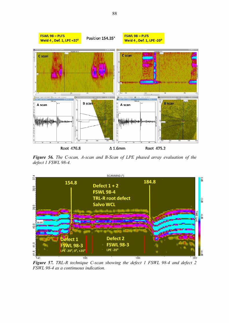
88
Figure 56. The C-scan, A-scan and B-Scan of LPE phased array evaluation of the defect 1 FSWL 98-4.
Figure 57. TRL-R technique C-scan showing the defect 1 FSWL 98-4 and defect 2 FSWL 98-4 as a continuous indication.
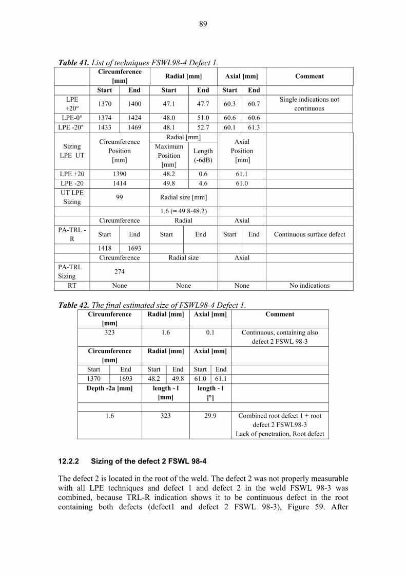
89
Table 41. List of techniques FSWL98-4 Defect 1.
Circumference
[mm] Radial [mm] Axial [mm] Comment
Start End Start End Start End
LPE +20°
1370 1400 47.1 47.7 60.3 60.7 Single indications not
continuous LPE-0° 1374 1424 48.0 51.0 60.6 60.6
LPE -20° 1433 1469 48.1 52.7 60.1 61.3
Sizing LPE UT
Circumference Position
[mm]
Radial [mm] Axial
Position [mm]
Maximum Position
[mm]
Length (-6dB)
LPE +20 1390 48.2 0.6 61.1
LPE -20 1414 49.8 4.6 61.0
UT LPE Sizing
99 Radial size [mm]
1.6 (= 49.8-48.2)
Circumference Radial Axial
PA-TRL -R
Start End Start End Start End Continuous surface defect
1418 1693
Circumference Radial size Axial
PA-TRL Sizing
274
RT None None None No indications
Table 42. The final estimated size of FSWL98-4 Defect 1.
Circumference [mm]
Radial [mm] Axial [mm] Comment
323 1.6 0.1 Continuous, containing also defect 2 FSWL 98-3
Circumference [mm]
Radial [mm] Axial [mm]
Start End Start End Start End 1370 1693 48.2 49.8 61.0 61.1 Depth -2a [mm] length - l
[mm] length - l
[]
1.6 323 29.9 Combined root defect 1 + root defect 2 FSWL98-3
Lack of penetration, Root defect
12.2.2 Sizing of the defect 2 FSWL 98-4
The defect 2 is located in the root of the weld. The defect 2 was not properly measurable with all LPE techniques and defect 1 and defect 2 in the weld FSWL 98-3 was combined, because TRL-R indication shows it to be continuous defect in the root containing both defects (defect1 and defect 2 FSWL 98-3), Figure 59. After
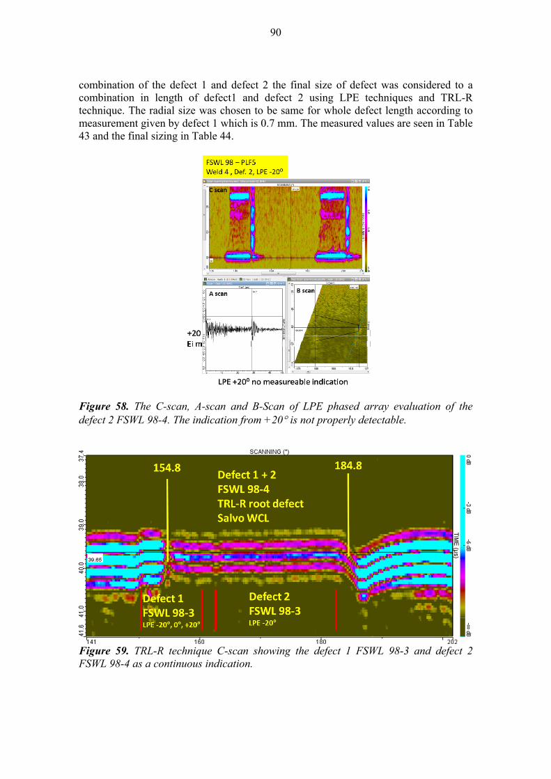
90
combination of the defect 1 and defect 2 the final size of defect was considered to a combination in length of defect1 and defect 2 using LPE techniques and TRL-R technique. The radial size was chosen to be same for whole defect length according to measurement given by defect 1 which is 0.7 mm. The measured values are seen in Table 43 and the final sizing in Table 44.
Figure 58. The C-scan, A-scan and B-Scan of LPE phased array evaluation of the defect 2 FSWL 98-4. The indication from +20 is not properly detectable.
Figure 59. TRL-R technique C-scan showing the defect 1 FSWL 98-3 and defect 2 FSWL 98-4 as a continuous indication.
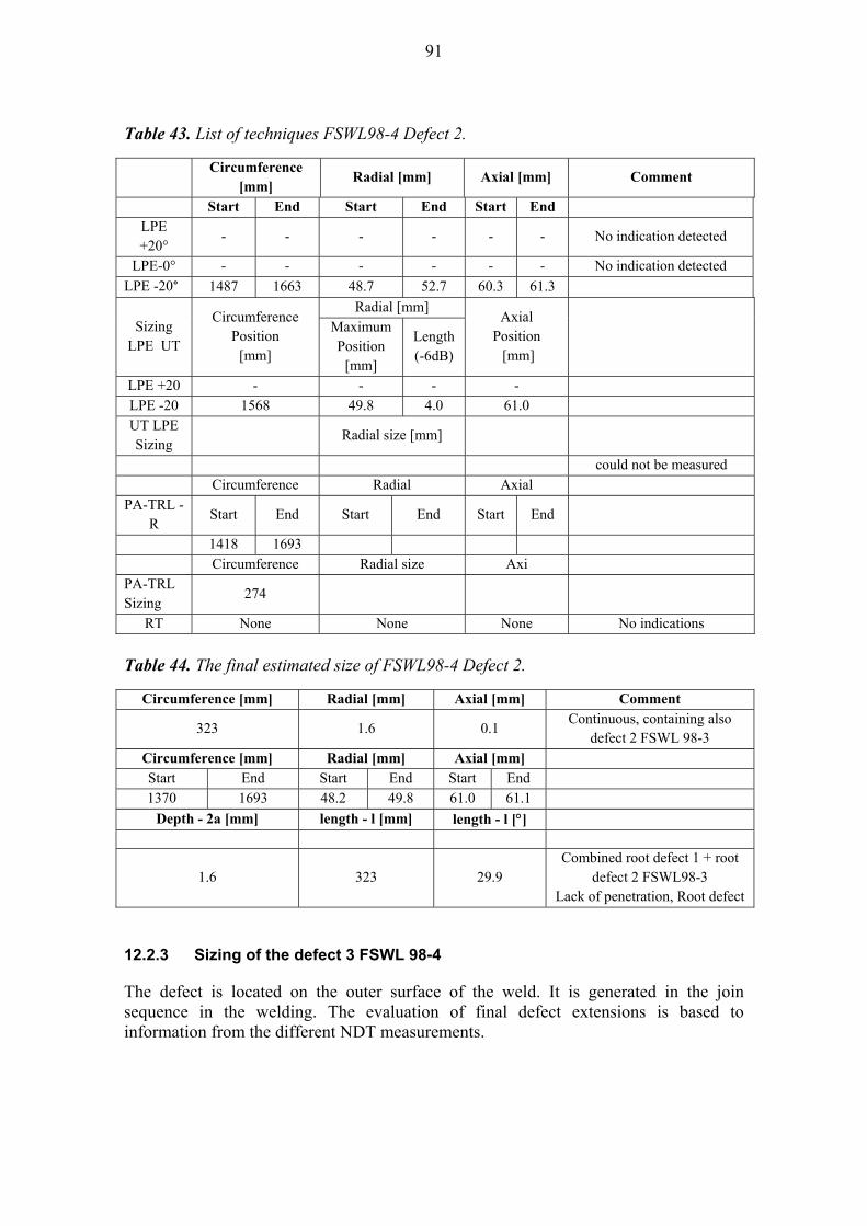
91
Table 43. List of techniques FSWL98-4 Defect 2.
Circumference
[mm] Radial [mm] Axial [mm] Comment
Start End Start End Start End
LPE +20°
- - - - - - No indication detected
LPE-0° - - - - - - No indication detected
LPE -20° 1487 1663 48.7 52.7 60.3 61.3
Sizing LPE UT
Circumference Position
[mm]
Radial [mm] Axial
Position [mm]
Maximum Position
[mm]
Length (-6dB)
LPE +20 - - - -
LPE -20 1568 49.8 4.0 61.0
UT LPE Sizing
Radial size [mm]
could not be measured
Circumference Radial Axial
PA-TRL -R
Start End Start End Start End
1418 1693
Circumference Radial size Axi
PA-TRL Sizing
274
RT None None None No indications
Table 44. The final estimated size of FSWL98-4 Defect 2.
Circumference [mm] Radial [mm] Axial [mm] Comment
323 1.6 0.1 Continuous, containing also
defect 2 FSWL 98-3
Circumference [mm] Radial [mm] Axial [mm]
Start End Start End Start End
1370 1693 48.2 49.8 61.0 61.1
Depth - 2a [mm] length - l [mm] length - l []
1.6 323 29.9 Combined root defect 1 + root
defect 2 FSWL98-3 Lack of penetration, Root defect
12.2.3 Sizing of the defect 3 FSWL 98-4
The defect is located on the outer surface of the weld. It is generated in the join sequence in the welding. The evaluation of final defect extensions is based to information from the different NDT measurements.
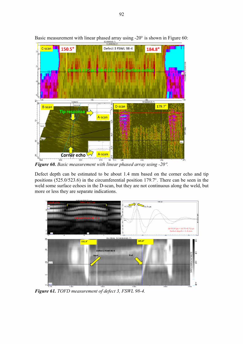
92
Basic measurement with linear phased array using -20 is shown in Figure 60:
Figure 60. Basic measurement with linear phased array using -20.
Defect depth can be estimated to be about 1.4 mm based on the corner echo and tip positions (525.0/523.6) in the circumferential position 179.7. There can be seen in the weld some surface echoes in the D-scan, but they are not continuous along the weld, but more or less they are separate indications.
Figure 61. TOFD measurement of defect 3, FSWL 98-4.
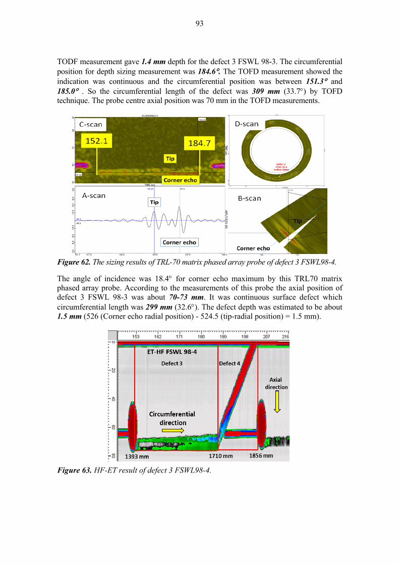
93
TODF measurement gave 1.4 mm depth for the defect 3 FSWL 98-3. The circumferential position for depth sizing measurement was 184.6. The TOFD measurement showed the indication was continuous and the circumferential position was between 151.3 and 185.0 . So the circumferential length of the defect was 309 mm (33.7) by TOFD technique. The probe centre axial position was 70 mm in the TOFD measurements.
Figure 62. The sizing results of TRL-70 matrix phased array probe of defect 3 FSWL98-4.
The angle of incidence was 18.4 for corner echo maximum by this TRL70 matrix phased array probe. According to the measurements of this probe the axial position of defect 3 FSWL 98-3 was about 70-73 mm. It was continuous surface defect which circumferential length was 299 mm (32.6). The defect depth was estimated to be about 1.5 mm (526 (Corner echo radial position) - 524.5 (tip-radial position) = 1.5 mm).
Figure 63. HF-ET result of defect 3 FSWL98-4.
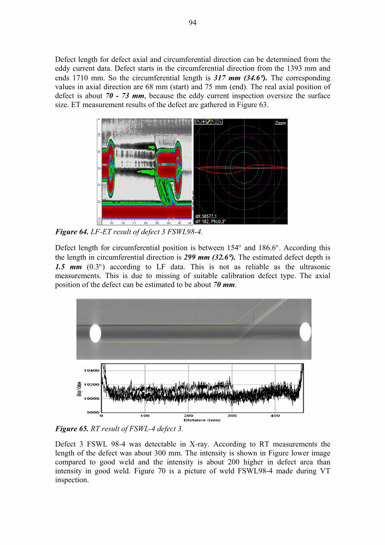
94
Defect length for defect axial and circumferential direction can be determined from the eddy current data. Defect starts in the circumferential direction from the 1393 mm and ends 1710 mm. So the circumferential length is 317 mm (34.6). The corresponding values in axial direction are 68 mm (start) and 75 mm (end). The real axial position of defect is about 70 - 73 mm, because the eddy current inspection oversize the surface size. ET measurement results of the defect are gathered in Figure 63.
Figure 64. LF-ET result of defect 3 FSWL98-4.
Defect length for circumferential position is between 154 and 186.6. According this the length in circumferential direction is 299 mm (32.6). The estimated defect depth is 1.5 mm (0.3) according to LF data. This is not as reliable as the ultrasonic measurements. This is due to missing of suitable calibration defect type. The axial position of the defect can be estimated to be about 70 mm.
Figure 65. RT result of FSWL-4 defect 3.
Defect 3 FSWL 98-4 was detectable in X-ray. According to RT measurements the length of the defect was about 300 mm. The intensity is shown in Figure lower image compared to good weld and the intensity is about 200 higher in defect area than intensity in good weld. Figure 70 is a picture of weld FSWL98-4 made during VT inspection.
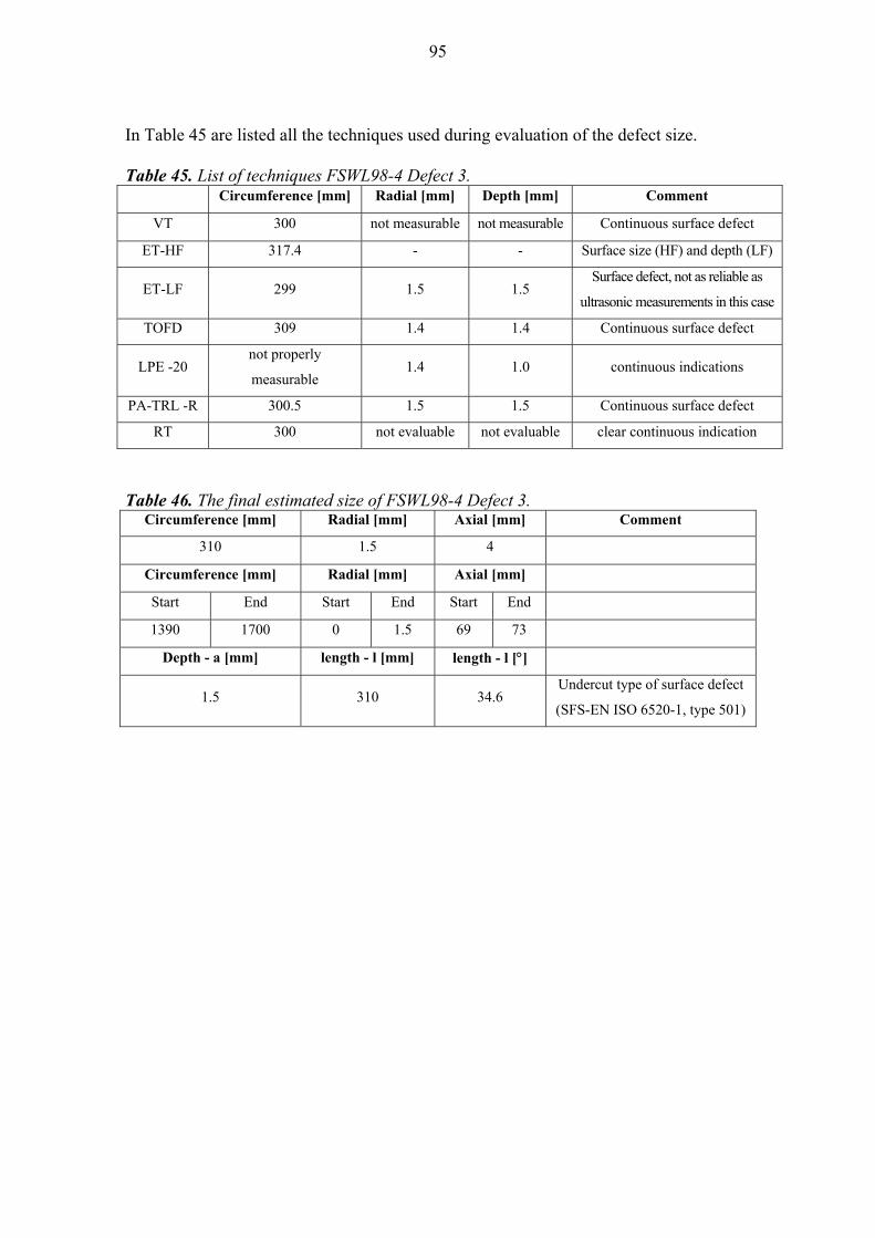
95
In Table 45 are listed all the techniques used during evaluation of the defect size. Table 45. List of techniques FSWL98-4 Defect 3.
Circumference [mm] Radial [mm] Depth [mm] Comment
VT 300 not measurable not measurable Continuous surface defect
ET-HF 317.4 - - Surface size (HF) and depth (LF)
ET-LF 299 1.5 1.5 Surface defect, not as reliable as
ultrasonic measurements in this case
TOFD 309 1.4 1.4 Continuous surface defect
LPE -20 not properly
measurable 1.4 1.0 continuous indications
PA-TRL -R 300.5 1.5 1.5 Continuous surface defect
RT 300 not evaluable not evaluable clear continuous indication
Table 46. The final estimated size of FSWL98-4 Defect 3.
Circumference [mm] Radial [mm] Axial [mm] Comment
310 1.5 4
Circumference [mm] Radial [mm] Axial [mm]
Start End Start End Start End
1390 1700 0 1.5 69 73
Depth - a [mm] length - l [mm] length - l []
1.5 310 34.6 Undercut type of surface defect
(SFS-EN ISO 6520-1, type 501)
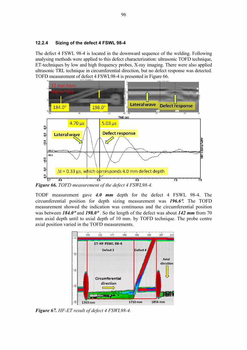
96
12.2.4 Sizing of the defect 4 FSWL 98-4
The defect 4 FSWL 98-4 is located in the downward sequence of the welding. Following analysing methods were applied to this defect characterization: ultrasonic TOFD technique, ET-techniques by low and high frequency probes, X-ray imaging. There were also applied ultrasonic TRL technique in circumferential direction, but no defect response was detected. TOFD measurement of defect 4 FSWL98-4 is presented in Figure 66.
Figure 66. TOFD measurement of the defect 4 FSWL98-4.
TODF measurement gave 4.0 mm depth for the defect 4 FSWL 98-4. The circumferential position for depth sizing measurement was 196.6. The TOFD measurement showed the indication was continuous and the circumferential position was between 184.0 and 198.0 . So the length of the defect was about 142 mm from 70 mm axial depth until to axial depth of 10 mm. by TOFD technique. The probe centre axial position varied in the TOFD measurements.
Figure 67. HF-ET result of defect 4 FSWL98-4.
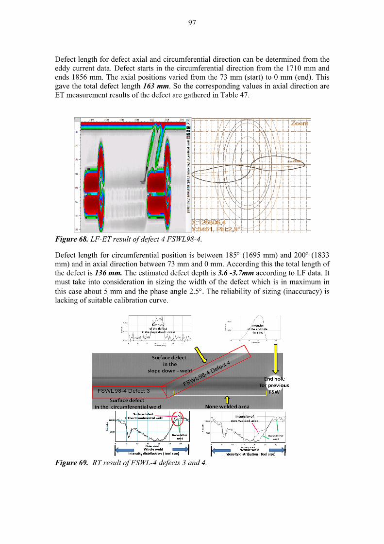
97
Defect length for defect axial and circumferential direction can be determined from the eddy current data. Defect starts in the circumferential direction from the 1710 mm and ends 1856 mm. The axial positions varied from the 73 mm (start) to 0 mm (end). This gave the total defect length 163 mm. So the corresponding values in axial direction are ET measurement results of the defect are gathered in Table 47.
Figure 68. LF-ET result of defect 4 FSWL98-4.
Defect length for circumferential position is between 185 (1695 mm) and 200 (1833 mm) and in axial direction between 73 mm and 0 mm. According this the total length of the defect is 136 mm. The estimated defect depth is 3.6 -3.7mm according to LF data. It must take into consideration in sizing the width of the defect which is in maximum in this case about 5 mm and the phase angle 2.5. The reliability of sizing (inaccuracy) is lacking of suitable calibration curve.
Figure 69. RT result of FSWL-4 defects 3 and 4.
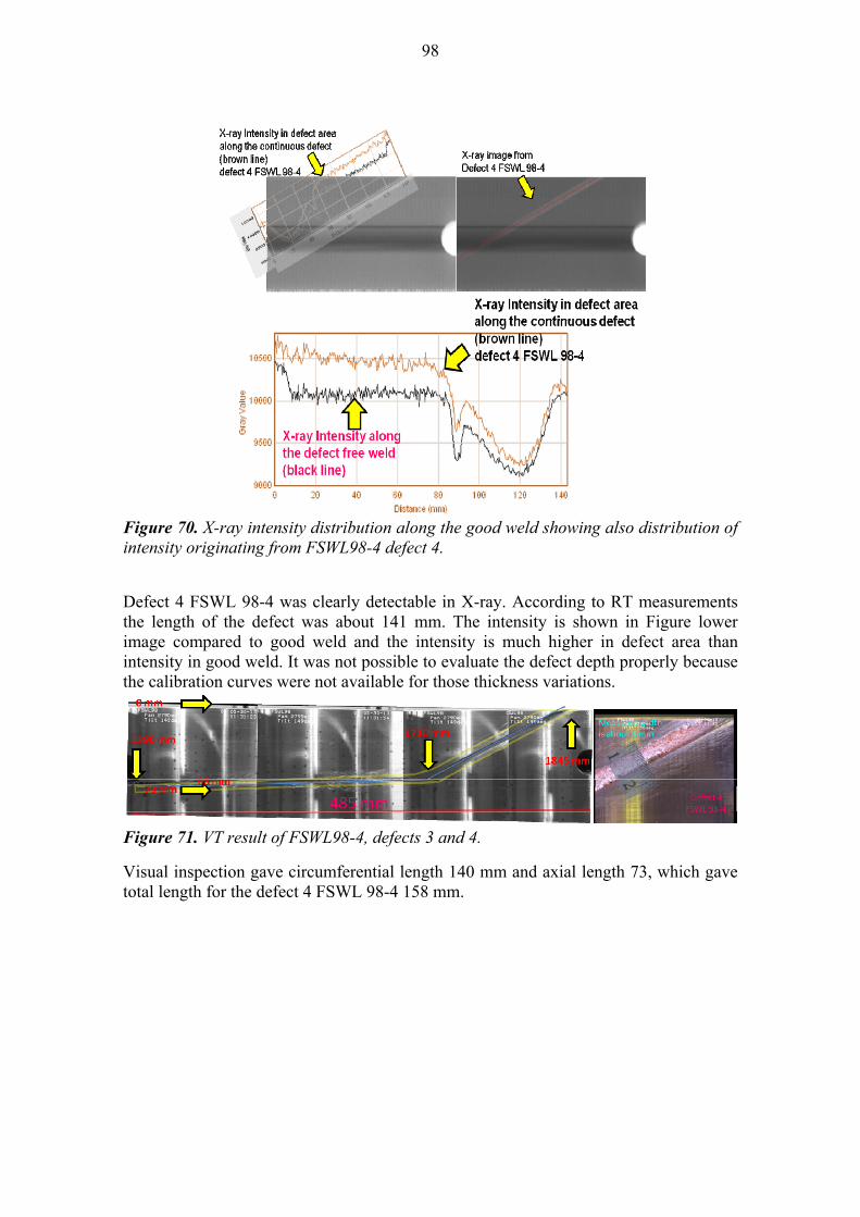
98
Figure 70. X-ray intensity distribution along the good weld showing also distribution of intensity originating from FSWL98-4 defect 4.
Defect 4 FSWL 98-4 was clearly detectable in X-ray. According to RT measurements the length of the defect was about 141 mm. The intensity is shown in Figure lower image compared to good weld and the intensity is much higher in defect area than intensity in good weld. It was not possible to evaluate the defect depth properly because the calibration curves were not available for those thickness variations.
Figure 71. VT result of FSWL98-4, defects 3 and 4.
Visual inspection gave circumferential length 140 mm and axial length 73, which gave total length for the defect 4 FSWL 98-4 158 mm.
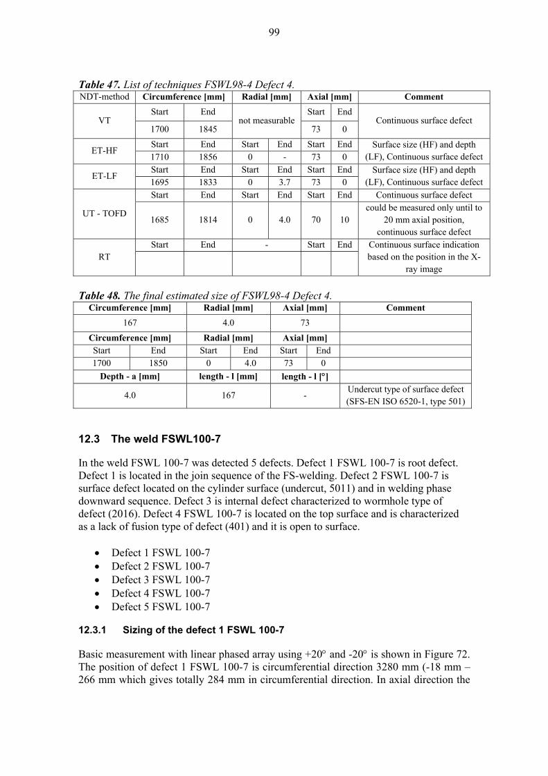
99
Table 47. List of techniques FSWL98-4 Defect 4. NDT-method Circumference [mm] Radial [mm] Axial [mm] Comment
VT Start End
not measurable Start End
Continuous surface defect 1700 1845 73 0
ET-HF Start End Start End Start End Surface size (HF) and depth
(LF), Continuous surface defect 1710 1856 0 - 73 0
ET-LF Start End Start End Start End Surface size (HF) and depth
(LF), Continuous surface defect 1695 1833 0 3.7 73 0
UT - TOFD
Start End Start End Start End Continuous surface defect
1685 1814 0 4.0 70 10 could be measured only until to
20 mm axial position, continuous surface defect
RT Start End - Start End Continuous surface indication
based on the position in the X-ray image
Table 48. The final estimated size of FSWL98-4 Defect 4.
Circumference [mm] Radial [mm] Axial [mm] Comment
167 4.0 73
Circumference [mm] Radial [mm] Axial [mm]
Start End Start End Start End
1700 1850 0 4.0 73 0
Depth - a [mm] length - l [mm] length - l []
4.0 167 - Undercut type of surface defect (SFS-EN ISO 6520-1, type 501)
12.3 The weld FSWL100-7
In the weld FSWL 100-7 was detected 5 defects. Defect 1 FSWL 100-7 is root defect. Defect 1 is located in the join sequence of the FS-welding. Defect 2 FSWL 100-7 is surface defect located on the cylinder surface (undercut, 5011) and in welding phase downward sequence. Defect 3 is internal defect characterized to wormhole type of defect (2016). Defect 4 FSWL 100-7 is located on the top surface and is characterized as a lack of fusion type of defect (401) and it is open to surface.
Defect 1 FSWL 100-7 Defect 2 FSWL 100-7 Defect 3 FSWL 100-7 Defect 4 FSWL 100-7 Defect 5 FSWL 100-7
12.3.1 Sizing of the defect 1 FSWL 100-7
Basic measurement with linear phased array using +20 and -20 is shown in Figure 72. The position of defect 1 FSWL 100-7 is circumferential direction 3280 mm (-18 mm – 266 mm which gives totally 284 mm in circumferential direction. In axial direction the
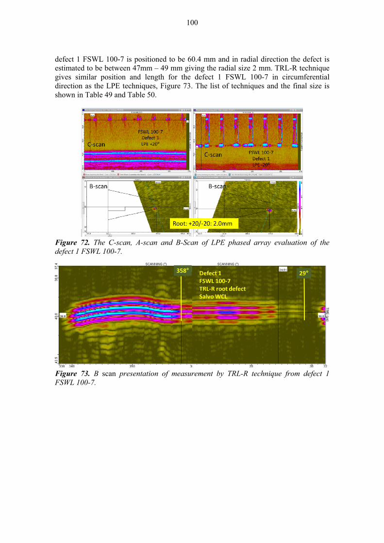
100
defect 1 FSWL 100-7 is positioned to be 60.4 mm and in radial direction the defect is estimated to be between 47mm – 49 mm giving the radial size 2 mm. TRL-R technique gives similar position and length for the defect 1 FSWL 100-7 in circumferential direction as the LPE techniques, Figure 73. The list of techniques and the final size is shown in Table 49 and Table 50.
Figure 72. The C-scan, A-scan and B-Scan of LPE phased array evaluation of the defect 1 FSWL 100-7.
Figure 73. B scan presentation of measurement by TRL-R technique from defect 1 FSWL 100-7.
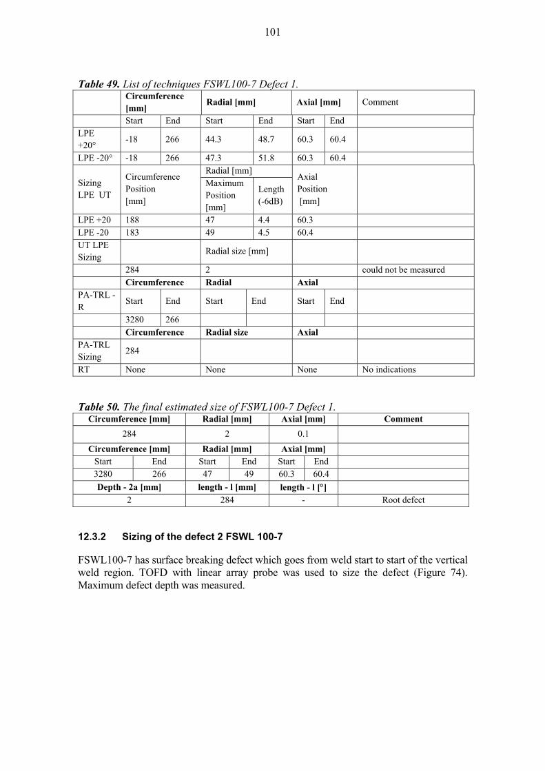
101
Table 49. List of techniques FSWL100-7 Defect 1.
Circumference [mm]
Radial [mm] Axial [mm] Comment
Start End Start End Start End LPE +20°
-18 266 44.3 48.7 60.3 60.4
LPE -20° -18 266 47.3 51.8 60.3 60.4
Sizing LPE UT
Circumference Position [mm]
Radial [mm] Axial Position [mm]
Maximum Position [mm]
Length (-6dB)
LPE +20 188 47 4.4 60.3 LPE -20 183 49 4.5 60.4 UT LPE Sizing
Radial size [mm]
284 2 could not be measured Circumference Radial Axial PA-TRL -R
Start End Start End Start End
3280 266 Circumference Radial size Axial PA-TRL Sizing
284
RT None None None No indications
Table 50. The final estimated size of FSWL100-7 Defect 1. Circumference [mm] Radial [mm] Axial [mm] Comment
284 2 0.1
Circumference [mm] Radial [mm] Axial [mm]
Start End Start End Start End
3280 266 47 49 60.3 60.4
Depth - 2a [mm] length - l [mm] length - l []
2 284 - Root defect
12.3.2 Sizing of the defect 2 FSWL 100-7
FSWL100-7 has surface breaking defect which goes from weld start to start of the vertical weld region. TOFD with linear array probe was used to size the defect (Figure 74). Maximum defect depth was measured.
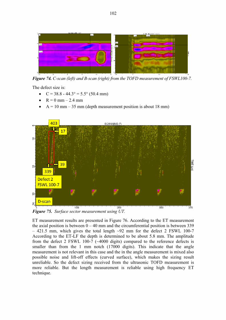
102
Figure 74. C-scan (left) and B-scan (right) from the TOFD measurement of FSWL100-7.
The defect size is:
C = 38.8 - 44.3° = 5.5° (50.4 mm)
R = 0 mm – 2.4 mm
A = 10 mm – 35 mm (depth measurement position is about 18 mm)
Figure 75. Surface sector measurement using UT.
ET measurement results are presented in Figure 76. According to the ET measurement the axial position is between 0 – 40 mm and the circumferential position is between 339 – 421.5 mm, which gives the total length ~92 mm for the defect 2 FSWL 100-7 According to the ET-LF the depth is determined to be about 5.8 mm. The amplitude from the defect 2 FSWL 100-7 (~4000 digits) compared to the reference defects is smaller than from the 1 mm notch (17000 digits). This indicate that the angle measurement is not relevant in this case and the in the angle measurement is mixed also possible noise and lift-off effects (curved surface), which makes the sizing result unreliable. So the defect sizing received from the ultrasonic TOFD measurement is more reliable. But the length measurement is reliable using high frequency ET technique.
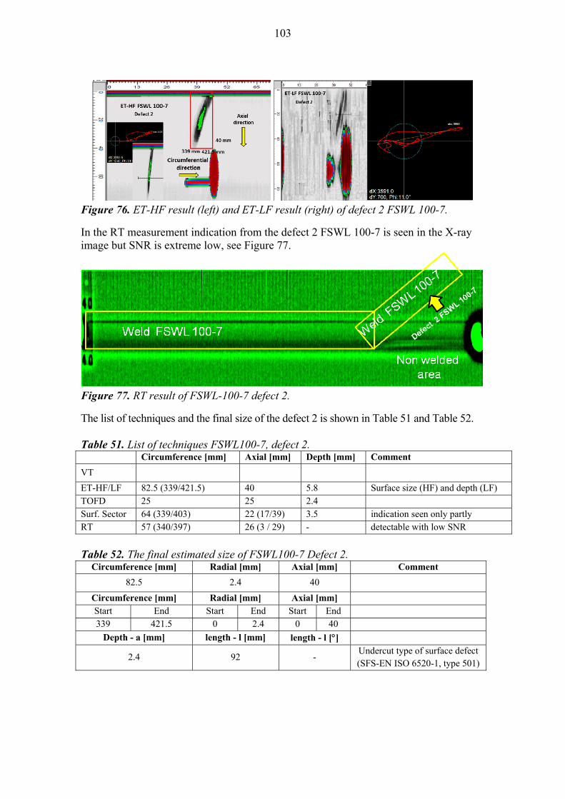
103
Figure 76. ET-HF result (left) and ET-LF result (right) of defect 2 FSWL 100-7.
In the RT measurement indication from the defect 2 FSWL 100-7 is seen in the X-ray image but SNR is extreme low, see Figure 77.
Figure 77. RT result of FSWL-100-7 defect 2.
The list of techniques and the final size of the defect 2 is shown in Table 51 and Table 52. Table 51. List of techniques FSWL100-7, defect 2. Circumference [mm] Axial [mm] Depth [mm] Comment
VT
ET-HF/LF 82.5 (339/421.5) 40 5.8 Surface size (HF) and depth (LF) TOFD 25 25 2.4 Surf. Sector 64 (339/403) 22 (17/39) 3.5 indication seen only partly RT 57 (340/397) 26 (3 / 29) - detectable with low SNR
Table 52. The final estimated size of FSWL100-7 Defect 2.
Circumference [mm] Radial [mm] Axial [mm] Comment
82.5 2.4 40
Circumference [mm] Radial [mm] Axial [mm]
Start End Start End Start End
339 421.5 0 2.4 0 40
Depth - a [mm] length - l [mm] length - l []
2.4 92 - Undercut type of surface defect (SFS-EN ISO 6520-1, type 501)
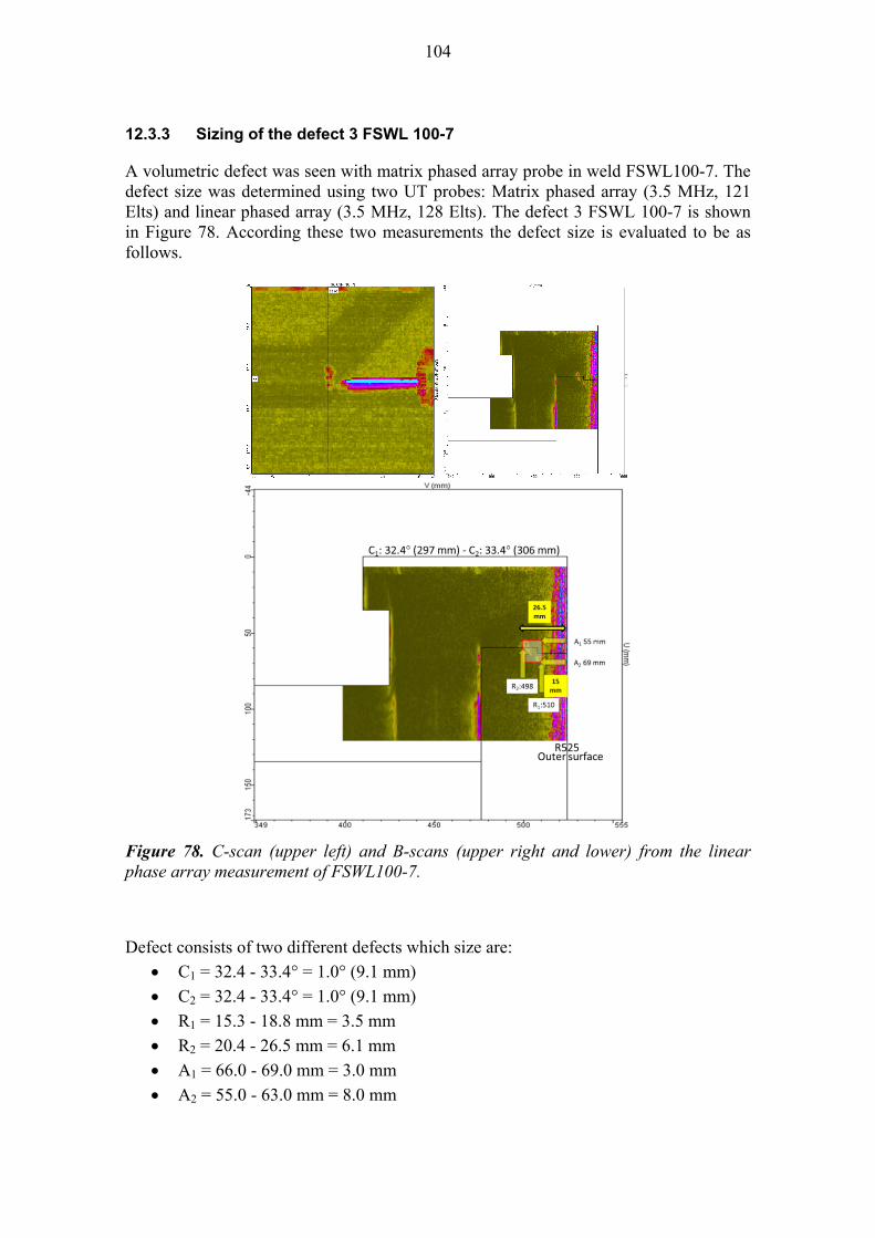
104
12.3.3 Sizing of the defect 3 FSWL 100-7
A volumetric defect was seen with matrix phased array probe in weld FSWL100-7. The defect size was determined using two UT probes: Matrix phased array (3.5 MHz, 121 Elts) and linear phased array (3.5 MHz, 128 Elts). The defect 3 FSWL 100-7 is shown in Figure 78. According these two measurements the defect size is evaluated to be as follows.
Figure 78. C-scan (upper left) and B-scans (upper right and lower) from the linear phase array measurement of FSWL100-7.
Defect consists of two different defects which size are:
C1 = 32.4 - 33.4° = 1.0° (9.1 mm)
C2 = 32.4 - 33.4° = 1.0° (9.1 mm)
R1 = 15.3 - 18.8 mm = 3.5 mm
R2 = 20.4 - 26.5 mm = 6.1 mm
A1 = 66.0 - 69.0 mm = 3.0 mm
A2 = 55.0 - 63.0 mm = 8.0 mm
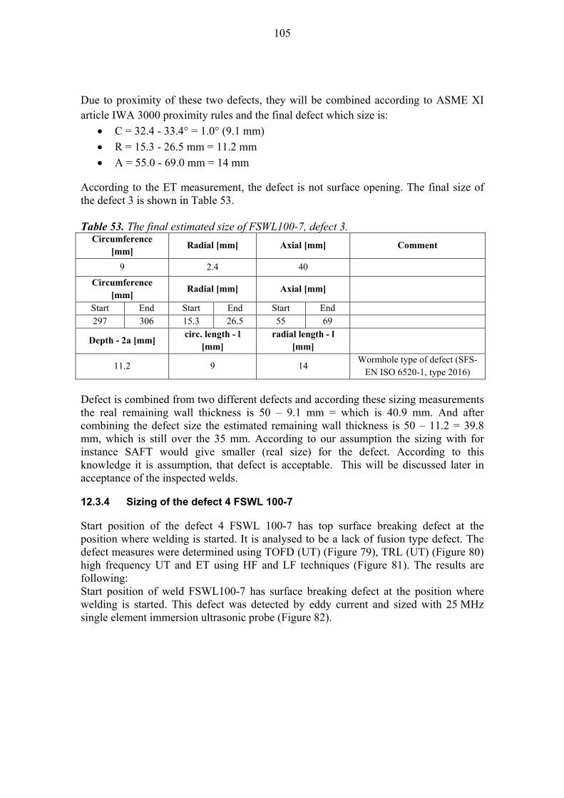
105
Due to proximity of these two defects, they will be combined according to ASME XI article IWA 3000 proximity rules and the final defect which size is:
C = 32.4 - 33.4° = 1.0° (9.1 mm)
R = 15.3 - 26.5 mm = 11.2 mm
A = 55.0 - 69.0 mm = 14 mm
According to the ET measurement, the defect is not surface opening. The final size of the defect 3 is shown in Table 53. Table 53. The final estimated size of FSWL100-7, defect 3.
Circumference [mm]
Radial [mm] Axial [mm] Comment
9 2.4 40
Circumference [mm]
Radial [mm] Axial [mm]
Start End Start End Start End
297 306 15.3 26.5 55 69
Depth - 2a [mm] circ. length - l
[mm] radial length - l
[mm]
11.2 9 14 Wormhole type of defect (SFS-
EN ISO 6520-1, type 2016)
Defect is combined from two different defects and according these sizing measurements the real remaining wall thickness is 50 – 9.1 mm = which is 40.9 mm. And after combining the defect size the estimated remaining wall thickness is 50 – 11.2 = 39.8 mm, which is still over the 35 mm. According to our assumption the sizing with for instance SAFT would give smaller (real size) for the defect. According to this knowledge it is assumption, that defect is acceptable. This will be discussed later in acceptance of the inspected welds.
12.3.4 Sizing of the defect 4 FSWL 100-7
Start position of the defect 4 FSWL 100-7 has top surface breaking defect at the position where welding is started. It is analysed to be a lack of fusion type defect. The defect measures were determined using TOFD (UT) (Figure 79), TRL (UT) (Figure 80) high frequency UT and ET using HF and LF techniques (Figure 81). The results are following: Start position of weld FSWL100-7 has surface breaking defect at the position where welding is started. This defect was detected by eddy current and sized with 25 MHz single element immersion ultrasonic probe (Figure 82).
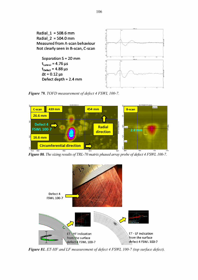
106
Figure 79. TOFD measurement of defect 4 FSWL 100-7.
Figure 80. The sizing results of TRL-70 matrix phased array probe of defect 4 FSWL 100-7.
Figure 81. ET-HF and LF measurement of defect 4 FSWL 100-7 (top surface defect).
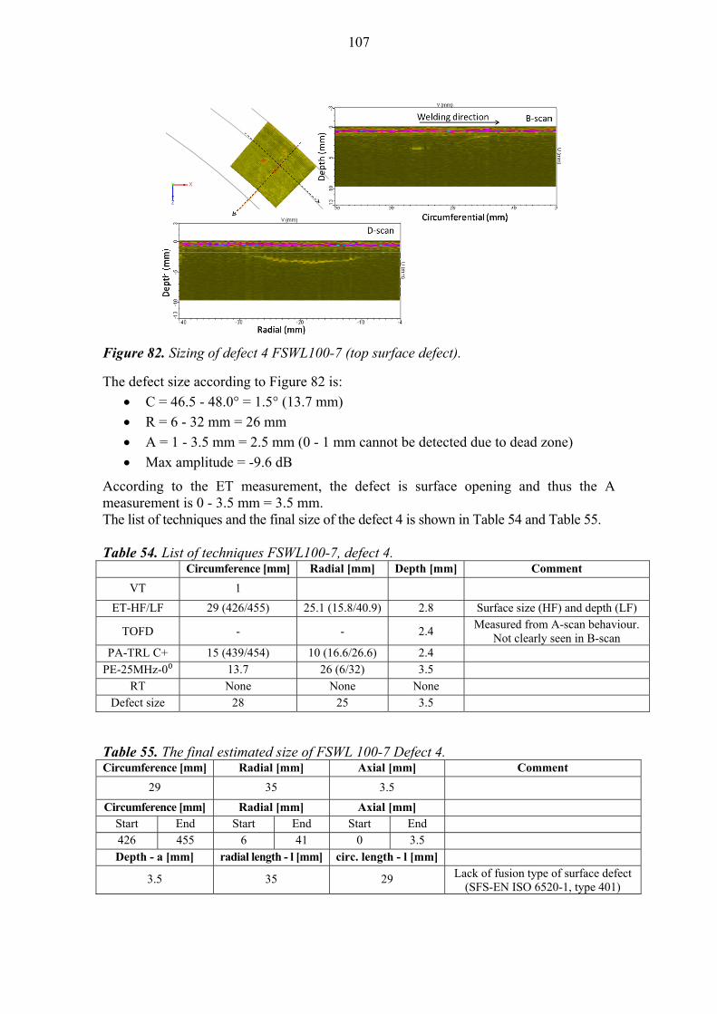
107
Figure 82. Sizing of defect 4 FSWL100-7 (top surface defect).
The defect size according to Figure 82 is:
C = 46.5 - 48.0° = 1.5° (13.7 mm)
R = 6 - 32 mm = 26 mm
A = 1 - 3.5 mm = 2.5 mm (0 - 1 mm cannot be detected due to dead zone)
Max amplitude = -9.6 dB
According to the ET measurement, the defect is surface opening and thus the A measurement is 0 - 3.5 mm = 3.5 mm. The list of techniques and the final size of the defect 4 is shown in Table 54 and Table 55. Table 54. List of techniques FSWL100-7, defect 4.
Circumference [mm] Radial [mm] Depth [mm] Comment
VT 1
ET-HF/LF 29 (426/455) 25.1 (15.8/40.9) 2.8 Surface size (HF) and depth (LF)
TOFD - - 2.4 Measured from A-scan behaviour.
Not clearly seen in B-scan PA-TRL C+ 15 (439/454) 10 (16.6/26.6) 2.4
PE-25MHz-0⁰ 13.7 26 (6/32) 3.5
RT None None None
Defect size 28 25 3.5
Table 55. The final estimated size of FSWL 100-7 Defect 4. Circumference [mm] Radial [mm] Axial [mm] Comment
29 35 3.5
Circumference [mm] Radial [mm] Axial [mm]
Start End Start End Start End
426 455 6 41 0 3.5
Depth - a [mm] radial length - l [mm] circ. length - l [mm]
3.5 35 29 Lack of fusion type of surface defect (SFS-EN ISO 6520-1, type 401)
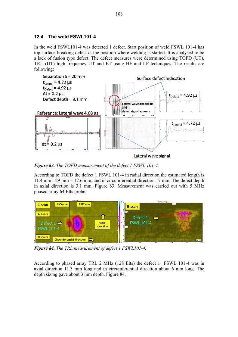
108
12.4 The weld FSWL101-4
In the weld FSWL101-4 was detected 1 defect. Start position of weld FSWL 101-4 has top surface breaking defect at the position where welding is started. It is analysed to be a lack of fusion type defect. The defect measures were determined using TOFD (UT), TRL (UT) high frequency UT and ET using HF and LF techniques. The results are following:
Figure 83. The TOFD measurement of the defect 1 FSWL 101-4.
According to TOFD the defect 1 FSWL 101-4 in radial direction the estimated length is 11.4 mm - 29 mm = 17.6 mm, and in circumferential direction 17 mm. The defect depth in axial direction is 3.1 mm, Figure 83. Measurement was carried out with 5 MHz phased array 64 Elts probe.
Figure 84. The TRL measurement of defect 1 FSWL101-4.
According to phased array TRL 2 MHz (128 Elts) the defect 1 FSWL 101-4 was in axial direction 11.3 mm long and in circumferential direction about 6 mm long. The depth sizing gave about 3 mm depth, Figure 84.
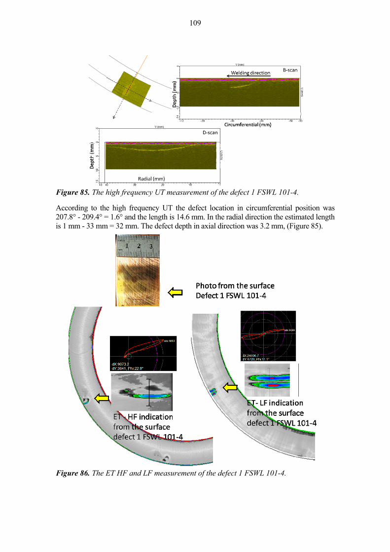
109
Figure 85. The high frequency UT measurement of the defect 1 FSWL 101-4.
According to the high frequency UT the defect location in circumferential position was 207.8° - 209.4° = 1.6° and the length is 14.6 mm. In the radial direction the estimated length is 1 mm - 33 mm = 32 mm. The defect depth in axial direction was 3.2 mm, (Figure 85).
Figure 86. The ET HF and LF measurement of the defect 1 FSWL 101-4.
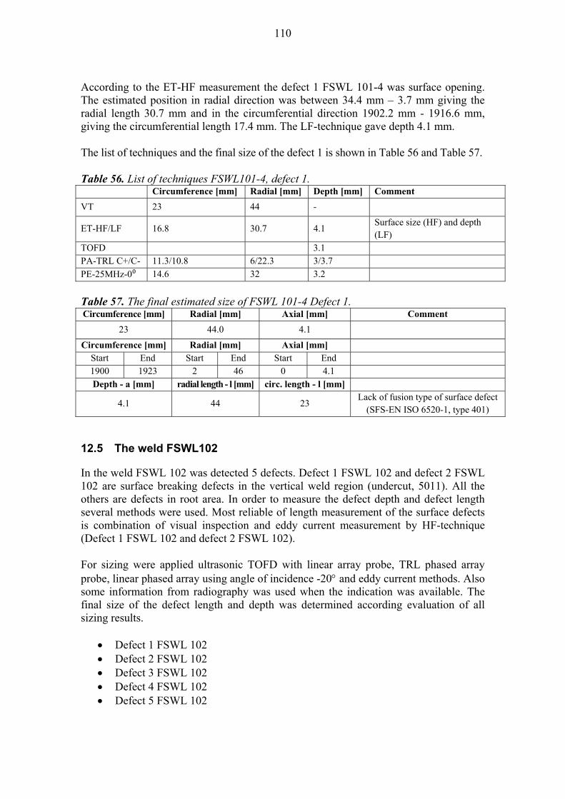
110
According to the ET-HF measurement the defect 1 FSWL 101-4 was surface opening. The estimated position in radial direction was between 34.4 mm – 3.7 mm giving the radial length 30.7 mm and in the circumferential direction 1902.2 mm - 1916.6 mm, giving the circumferential length 17.4 mm. The LF-technique gave depth 4.1 mm. The list of techniques and the final size of the defect 1 is shown in Table 56 and Table 57. Table 56. List of techniques FSWL101-4, defect 1. Circumference [mm] Radial [mm] Depth [mm] Comment
VT 23 44 -
ET-HF/LF 16.8 30.7 4.1 Surface size (HF) and depth (LF)
TOFD 3.1 PA-TRL C+/C- 11.3/10.8 6/22.3 3/3.7
PE-25MHz-0⁰ 14.6 32 3.2
Table 57. The final estimated size of FSWL 101-4 Defect 1. Circumference [mm] Radial [mm] Axial [mm] Comment
23 44.0 4.1
Circumference [mm] Radial [mm] Axial [mm]
Start End Start End Start End
1900 1923 2 46 0 4.1
Depth - a [mm] radial length - l [mm] circ. length - l [mm]
4.1 44 23 Lack of fusion type of surface defect
(SFS-EN ISO 6520-1, type 401)
12.5 The weld FSWL102
In the weld FSWL 102 was detected 5 defects. Defect 1 FSWL 102 and defect 2 FSWL 102 are surface breaking defects in the vertical weld region (undercut, 5011). All the others are defects in root area. In order to measure the defect depth and defect length several methods were used. Most reliable of length measurement of the surface defects is combination of visual inspection and eddy current measurement by HF-technique (Defect 1 FSWL 102 and defect 2 FSWL 102). For sizing were applied ultrasonic TOFD with linear array probe, TRL phased array probe, linear phased array using angle of incidence -20 and eddy current methods. Also some information from radiography was used when the indication was available. The final size of the defect length and depth was determined according evaluation of all sizing results.
Defect 1 FSWL 102 Defect 2 FSWL 102 Defect 3 FSWL 102 Defect 4 FSWL 102 Defect 5 FSWL 102
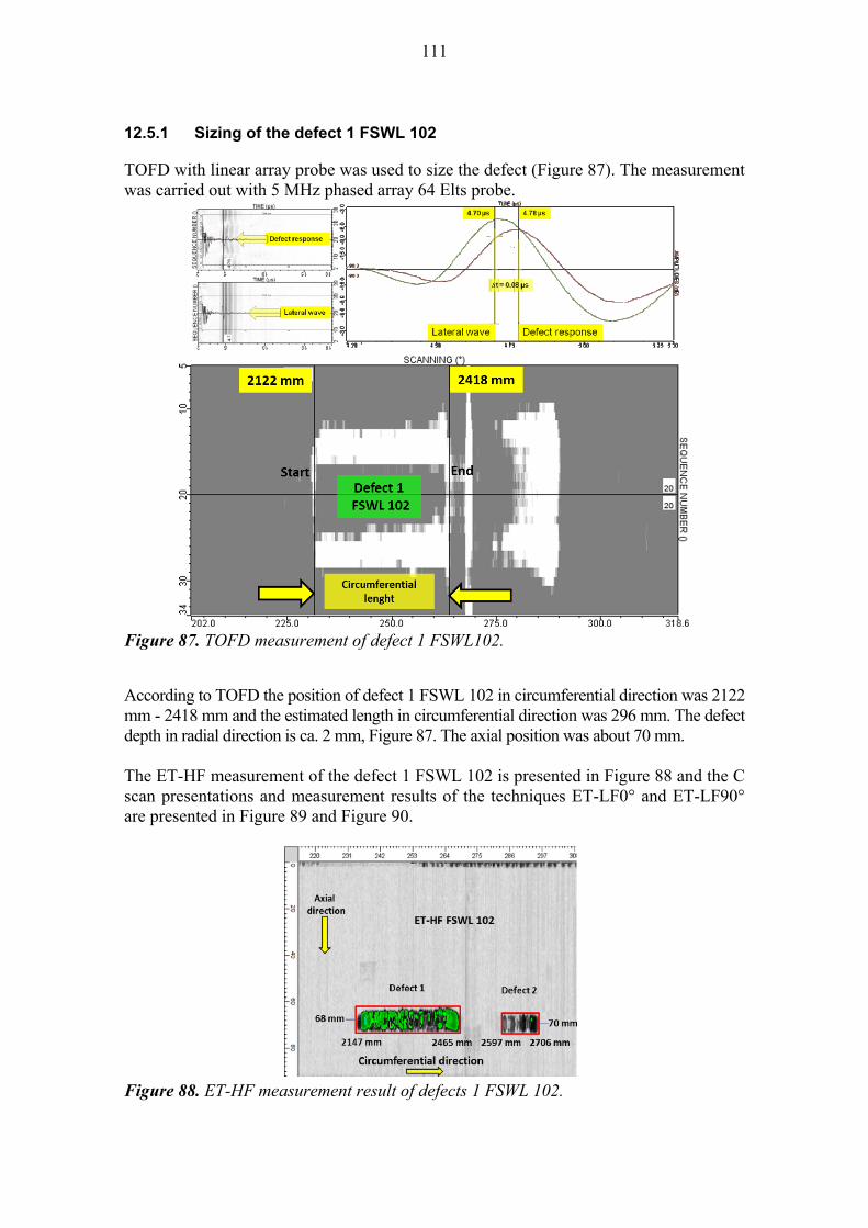
111
12.5.1 Sizing of the defect 1 FSWL 102
TOFD with linear array probe was used to size the defect (Figure 87). The measurement was carried out with 5 MHz phased array 64 Elts probe.
Figure 87. TOFD measurement of defect 1 FSWL102.
According to TOFD the position of defect 1 FSWL 102 in circumferential direction was 2122 mm - 2418 mm and the estimated length in circumferential direction was 296 mm. The defect depth in radial direction is ca. 2 mm, Figure 87. The axial position was about 70 mm. The ET-HF measurement of the defect 1 FSWL 102 is presented in Figure 88 and the C scan presentations and measurement results of the techniques ET-LF0° and ET-LF90° are presented in Figure 89 and Figure 90.
Figure 88. ET-HF measurement result of defects 1 FSWL 102.
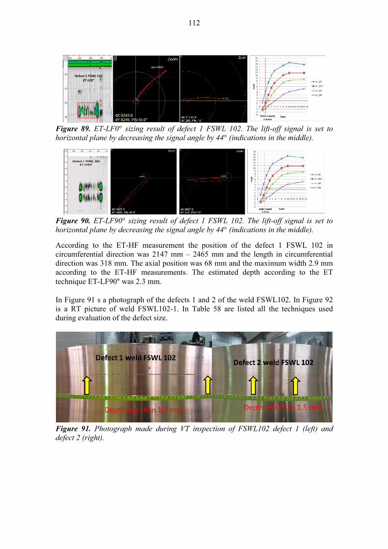
112
Figure 89. ET-LF0° sizing result of defect 1 FSWL 102. The lift-off signal is set to horizontal plane by decreasing the signal angle by 44° (indications in the middle).
Figure 90. ET-LF90° sizing result of defect 1 FSWL 102. The lift-off signal is set to horizontal plane by decreasing the signal angle by 44° (indications in the middle).
According to the ET-HF measurement the position of the defect 1 FSWL 102 in circumferential direction was 2147 mm – 2465 mm and the length in circumferential direction was 318 mm. The axial position was 68 mm and the maximum width 2.9 mm according to the ET-HF measurements. The estimated depth according to the ET technique ET-LF90° was 2.3 mm. In Figure 91 s a photograph of the defects 1 and 2 of the weld FSWL102. In Figure 92 is a RT picture of weld FSWL102-1. In Table 58 are listed all the techniques used during evaluation of the defect size.
Figure 91. Photograph made during VT inspection of FSWL102 defect 1 (left) and defect 2 (right).
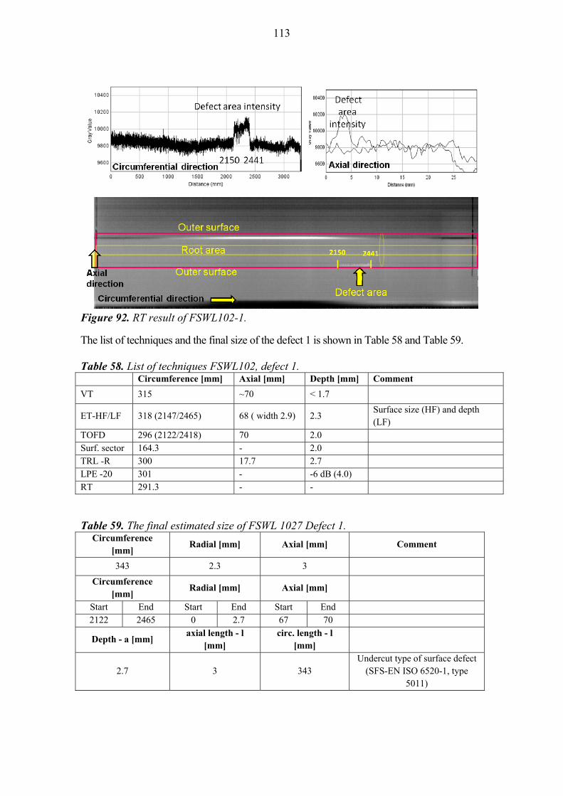
113
Figure 92. RT result of FSWL102-1.
The list of techniques and the final size of the defect 1 is shown in Table 58 and Table 59. Table 58. List of techniques FSWL102, defect 1. Circumference [mm] Axial [mm] Depth [mm] Comment
VT 315 ~70 < 1.7
ET-HF/LF 318 (2147/2465) 68 ( width 2.9) 2.3 Surface size (HF) and depth (LF)
TOFD 296 (2122/2418) 70 2.0 Surf. sector 164.3 - 2.0 TRL -R 300 17.7 2.7 LPE -20 301 - -6 dB (4.0) RT 291.3 - -
Table 59. The final estimated size of FSWL 1027 Defect 1. Circumference
[mm] Radial [mm] Axial [mm] Comment
343 2.3 3
Circumference [mm]
Radial [mm] Axial [mm]
Start End Start End Start End
2122 2465 0 2.7 67 70
Depth - a [mm] axial length - l
[mm] circ. length - l
[mm]
2.7 3 343 Undercut type of surface defect
(SFS-EN ISO 6520-1, type 5011)
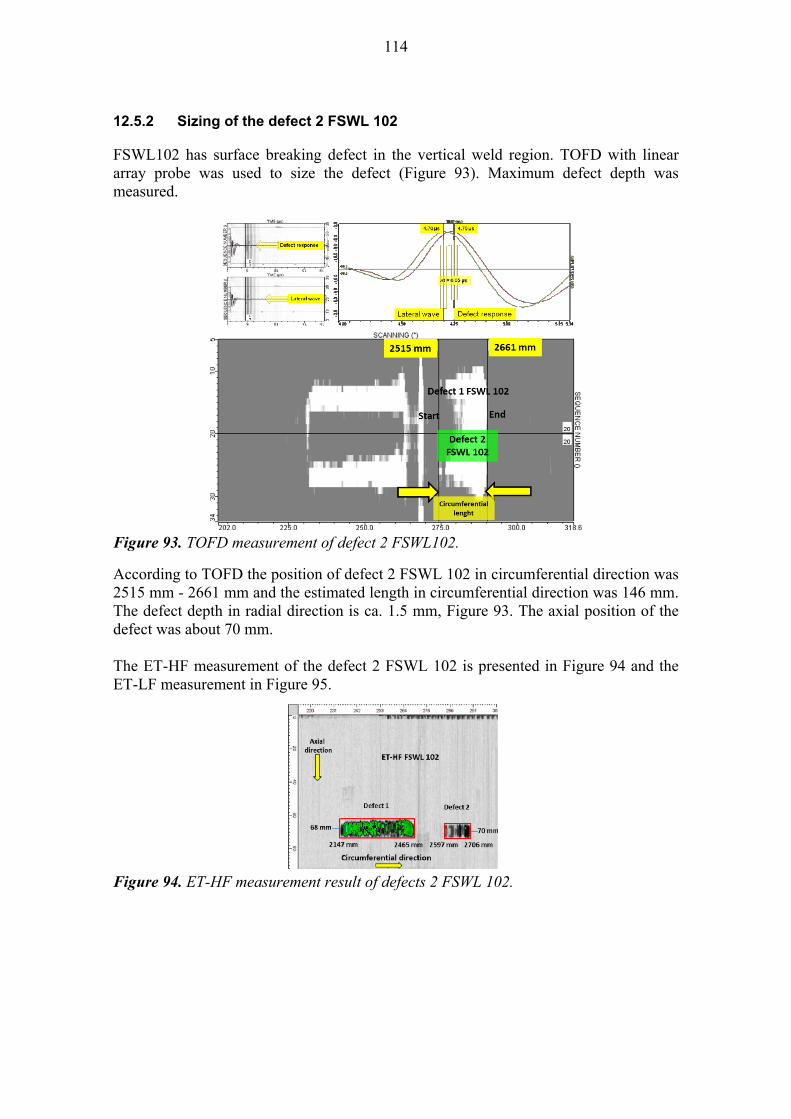
114
12.5.2 Sizing of the defect 2 FSWL 102
FSWL102 has surface breaking defect in the vertical weld region. TOFD with linear array probe was used to size the defect (Figure 93). Maximum defect depth was measured.
Figure 93. TOFD measurement of defect 2 FSWL102.
According to TOFD the position of defect 2 FSWL 102 in circumferential direction was 2515 mm - 2661 mm and the estimated length in circumferential direction was 146 mm. The defect depth in radial direction is ca. 1.5 mm, Figure 93. The axial position of the defect was about 70 mm. The ET-HF measurement of the defect 2 FSWL 102 is presented in Figure 94 and the ET-LF measurement in Figure 95.
Figure 94. ET-HF measurement result of defects 2 FSWL 102.
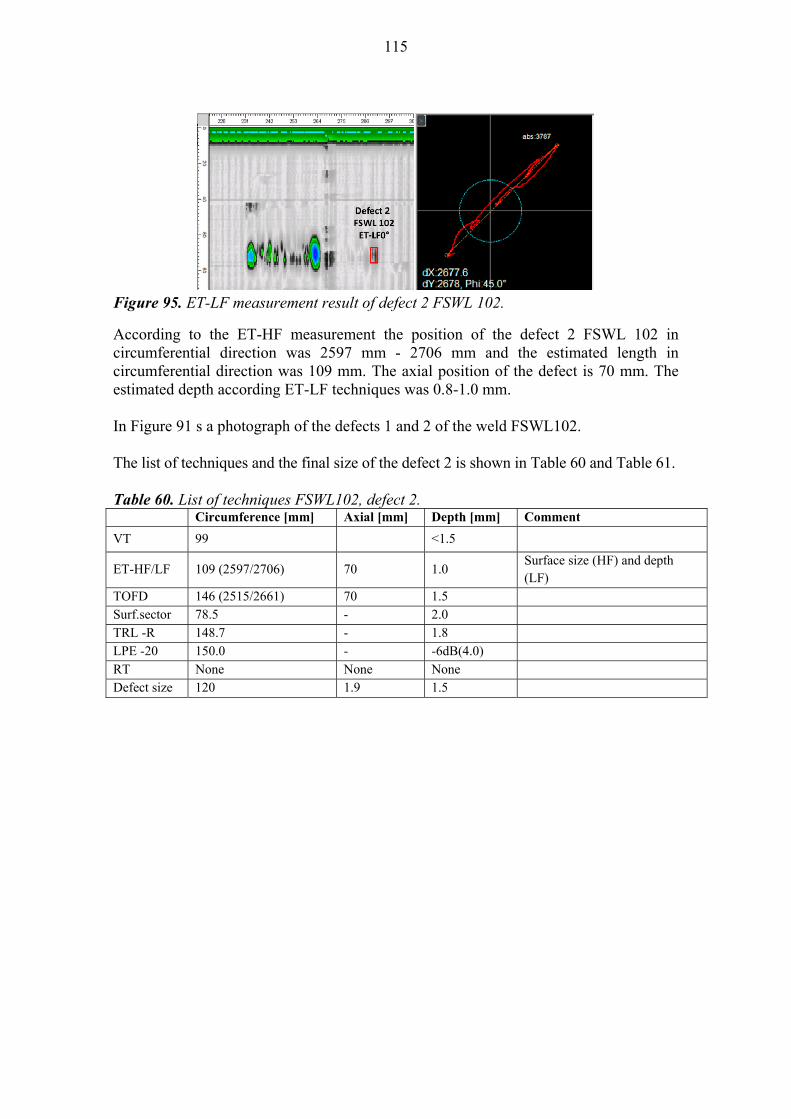
115
Figure 95. ET-LF measurement result of defect 2 FSWL 102.
According to the ET-HF measurement the position of the defect 2 FSWL 102 in circumferential direction was 2597 mm - 2706 mm and the estimated length in circumferential direction was 109 mm. The axial position of the defect is 70 mm. The estimated depth according ET-LF techniques was 0.8-1.0 mm. In Figure 91 s a photograph of the defects 1 and 2 of the weld FSWL102. The list of techniques and the final size of the defect 2 is shown in Table 60 and Table 61. Table 60. List of techniques FSWL102, defect 2. Circumference [mm] Axial [mm] Depth [mm] Comment
VT 99 <1.5
ET-HF/LF 109 (2597/2706) 70 1.0 Surface size (HF) and depth (LF)
TOFD 146 (2515/2661) 70 1.5 Surf.sector 78.5 - 2.0 TRL -R 148.7 - 1.8 LPE -20 150.0 - -6dB(4.0) RT None None None Defect size 120 1.9 1.5
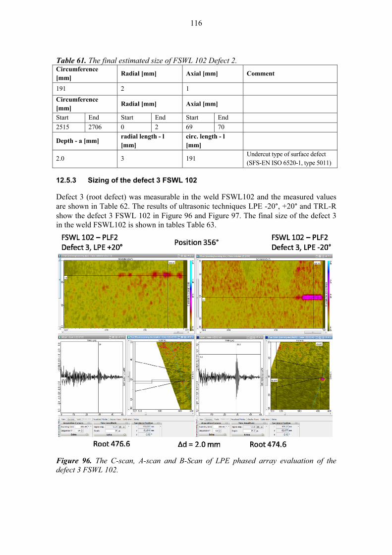
116
Table 61. The final estimated size of FSWL 102 Defect 2. Circumference [mm]
Radial [mm] Axial [mm] Comment
191 2 1
Circumference [mm]
Radial [mm] Axial [mm]
Start End Start End Start End
2515 2706 0 2 69 70
Depth - a [mm] radial length - l [mm]
circ. length - l [mm]
2.0 3 191 Undercut type of surface defect (SFS-EN ISO 6520-1, type 5011)
12.5.3 Sizing of the defect 3 FSWL 102
Defect 3 (root defect) was measurable in the weld FSWL102 and the measured values are shown in Table 62. The results of ultrasonic techniques LPE -20°, +20° and TRL-R show the defect 3 FSWL 102 in Figure 96 and Figure 97. The final size of the defect 3 in the weld FSWL102 is shown in tables Table 63.
Figure 96. The C-scan, A-scan and B-Scan of LPE phased array evaluation of the defect 3 FSWL 102.

117
Figure 97. TRL-R technique C-scan showing all detected defects in the weld FSWL 102.
The list of techniques of the defect 3 is shown in Table 62. Table 62. List of techniques FSWL102 Defect 3.
Circumference
[mm] Radial [mm] Axial [mm] Comment
Start End Start End Start End
LPE +20°
3147 277 46.4 49.2 60.5 61.6
LPE -20° 3182 907 49.0 53.0 60.0 60.0
Sizing LPE UT
Circumference Position
[mm]
Radial [mm] Axial
Position [mm]
Maximum Position
[mm]
Length (-6dB)
LPE +20 3262 48.4 2.8 61.6
LPE -20 3262 50.4 4.0 62.1
UT LPE Sizing
Radial size [mm]
1058 2.0 could not be measured
Circumference Radial Axial
PA-TRL -R
Start End Start End Start End
3196 909
Circumference Radial size Axial
PA-TRL Sizing
1012
RT None None None No indications
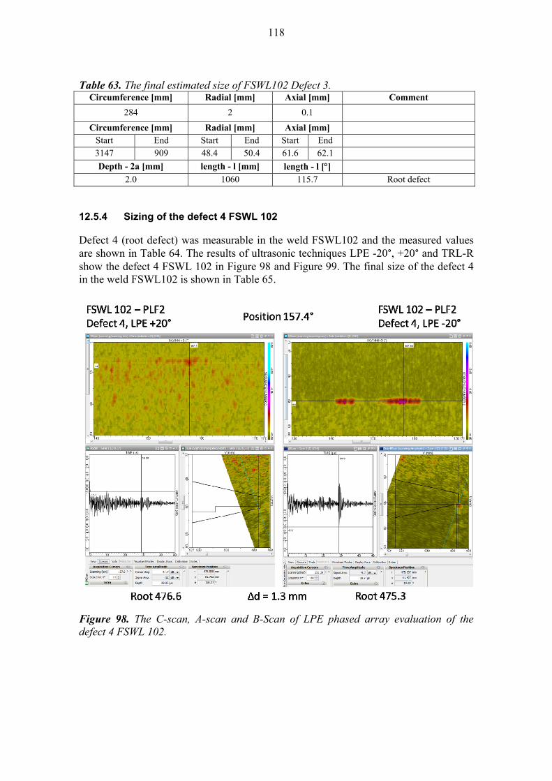
118
Table 63. The final estimated size of FSWL102 Defect 3. Circumference [mm] Radial [mm] Axial [mm] Comment
284 2 0.1
Circumference [mm] Radial [mm] Axial [mm]
Start End Start End Start End
3147 909 48.4 50.4 61.6 62.1
Depth - 2a [mm] length - l [mm] length - l []
2.0 1060 115.7 Root defect
12.5.4 Sizing of the defect 4 FSWL 102
Defect 4 (root defect) was measurable in the weld FSWL102 and the measured values are shown in Table 64. The results of ultrasonic techniques LPE -20°, +20° and TRL-R show the defect 4 FSWL 102 in Figure 98 and Figure 99. The final size of the defect 4 in the weld FSWL102 is shown in Table 65.
Figure 98. The C-scan, A-scan and B-Scan of LPE phased array evaluation of the defect 4 FSWL 102.
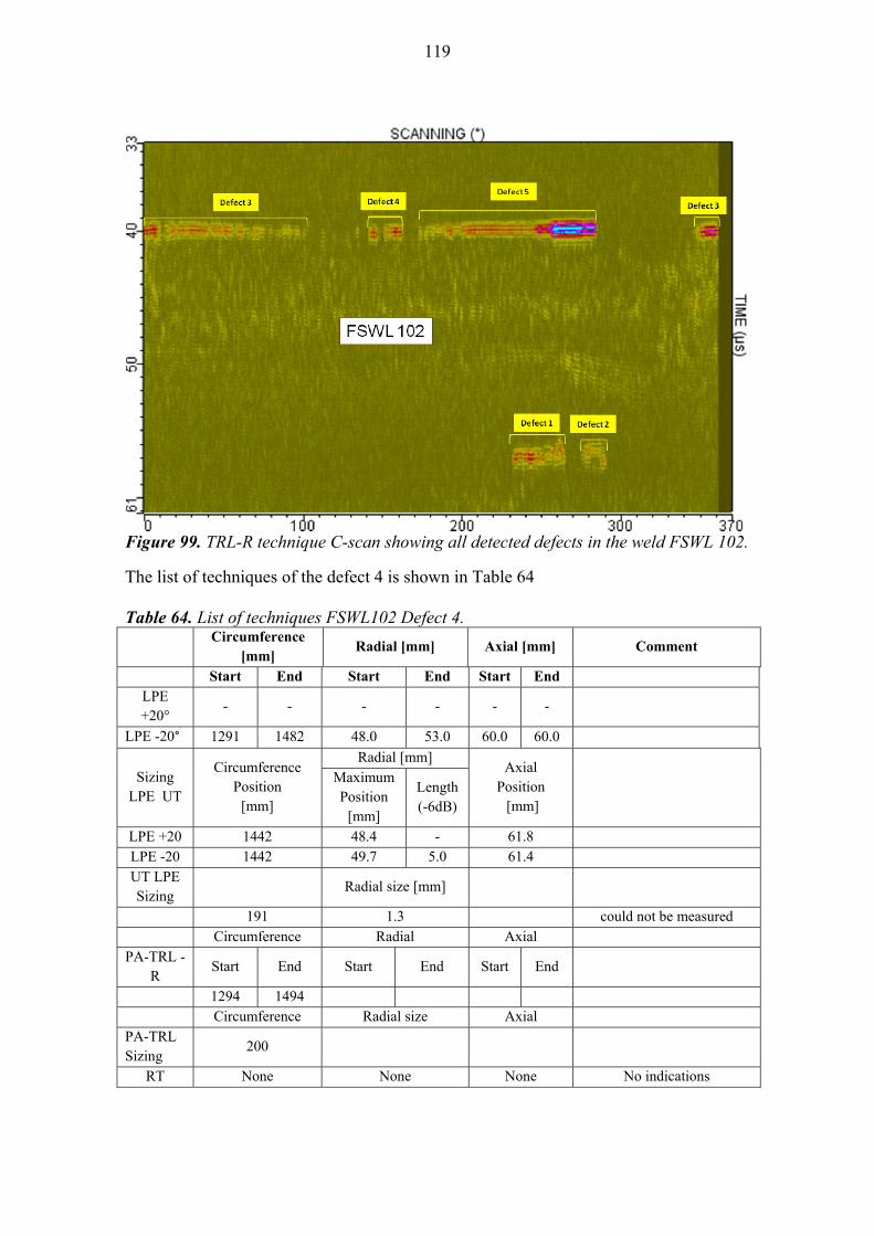
119
Figure 99. TRL-R technique C-scan showing all detected defects in the weld FSWL 102.
The list of techniques of the defect 4 is shown in Table 64 Table 64. List of techniques FSWL102 Defect 4.
Circumference
[mm] Radial [mm] Axial [mm] Comment
Start End Start End Start End
LPE +20°
- - - - - -
LPE -20° 1291 1482 48.0 53.0 60.0 60.0
Sizing LPE UT
Circumference Position
[mm]
Radial [mm] Axial
Position [mm]
Maximum Position
[mm]
Length (-6dB)
LPE +20 1442 48.4 - 61.8
LPE -20 1442 49.7 5.0 61.4
UT LPE Sizing
Radial size [mm]
191 1.3 could not be measured
Circumference Radial Axial
PA-TRL -R
Start End Start End Start End
1294 1494
Circumference Radial size Axial
PA-TRL Sizing
200
RT None None None No indications
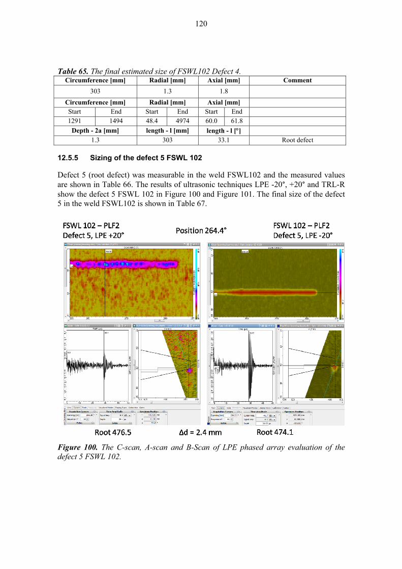
120
Table 65. The final estimated size of FSWL102 Defect 4.
Circumference [mm] Radial [mm] Axial [mm] Comment
303 1.3 1.8
Circumference [mm] Radial [mm] Axial [mm]
Start End Start End Start End
1291 1494 48.4 4974 60.0 61.8
Depth - 2a [mm] length - l [mm] length - l []
1.3 303 33.1 Root defect
12.5.5 Sizing of the defect 5 FSWL 102
Defect 5 (root defect) was measurable in the weld FSWL102 and the measured values are shown in Table 66. The results of ultrasonic techniques LPE -20°, +20° and TRL-R show the defect 5 FSWL 102 in Figure 100 and Figure 101. The final size of the defect 5 in the weld FSWL102 is shown in Table 67.
Figure 100. The C-scan, A-scan and B-Scan of LPE phased array evaluation of the defect 5 FSWL 102.
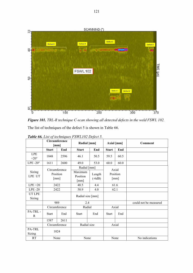
121
Figure 101. TRL-R technique C-scan showing all detected defects in the weld FSWL 102.
The list of techniques of the defect 5 is shown in Table 66. Table 66. List of techniques FSWL102 Defect 5.
Circumference
[mm] Radial [mm] Axial [mm] Comment
Start End Start End Start End
LPE +20°
1848 2596 46.1 50.5 59.5 60.5
LPE -20° 1611 2600 49.0 53.0 60.0 60.0
Sizing LPE UT
Circumference Position
[mm]
Radial [mm] Axial
Position [mm]
Maximum Position
[mm]
Length (-6dB)
LPE +20 2422 48.5 4.4 61.6
LPE -20 2422 50.9 4.0 62.1
UT LPE Sizing
Radial size [mm]
989 2.4 could not be measured
Circumference Radial Axial
PA-TRL -R
Start End Start End Start End
1587 2611
Circumference Radial size Axial
PA-TRL Sizing
1024
RT None None None No indications

122
Table 67. The final estimated size of FSWL102 Defect 5. Circumference [mm] Radial [mm] Axial [mm] Comment
1024 2.4 2.6
Circumference [mm] Radial [mm] Axial [mm]
Start End Start End Start End
1587 2611 48.5 50.9 59.5 62.1
Depth - 2a [mm] length - l [mm] length - l []
2.4 1024 111.8 Root defect
12.6 The weld FSWL103
In the weld FSWL 103 was detected 1 defect in root area, defect 1 FSWL 103. In order to measure the defect depth and defect length several methods were used. For sizing were applied ultrasonic TRL phased array probe, linear phased array using angle of incidence +20 and -20. The final size of the defect length and depth was determined according evaluation of all sizing results.
Defect 1 FSWL 103
12.6.1 Sizing of the defect 1 FSWL 103
Defect 1 (root defect) was measurable in the weld FSWL103 and the measured values are shown in Table 68. The results of ultrasonic techniques LPE -20°, +20° and TRL-R show the defect 1 FSWL 103 in Figure 102 and Figure 103. The final size of the defect 1 in the weld FSWL103 is shown in Table 69.
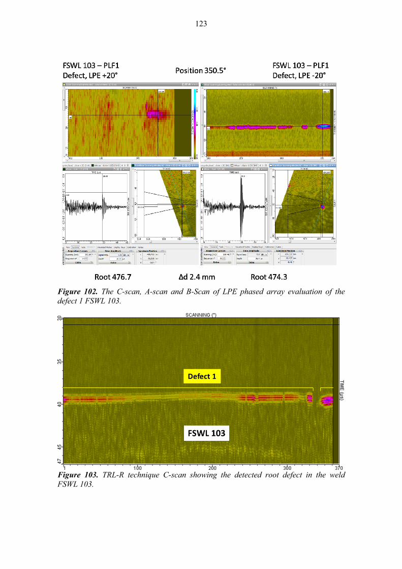
123
Figure 102. The C-scan, A-scan and B-Scan of LPE phased array evaluation of the defect 1 FSWL 103.
Figure 103. TRL-R technique C-scan showing the detected root defect in the weld FSWL 103.
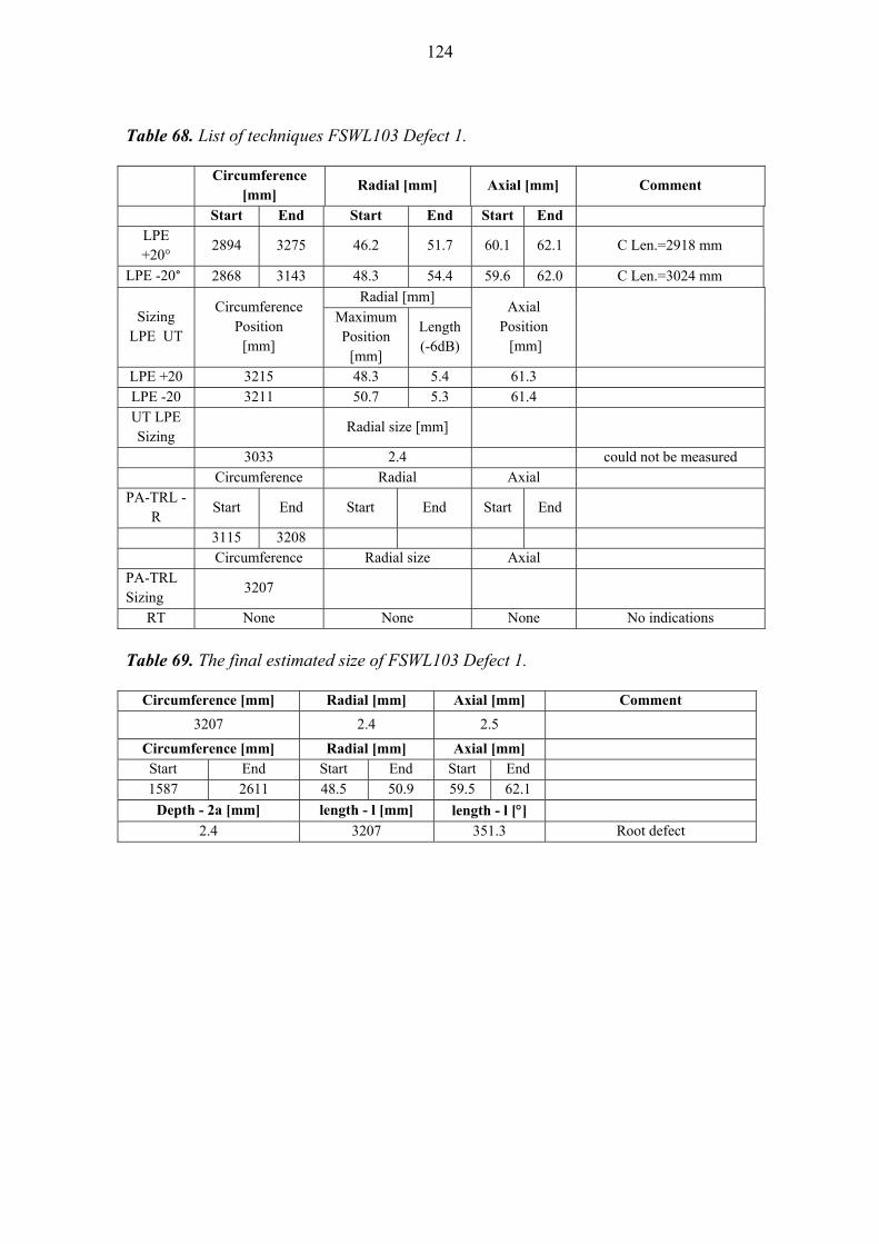
124
Table 68. List of techniques FSWL103 Defect 1.
Circumference
[mm] Radial [mm] Axial [mm] Comment
Start End Start End Start End
LPE +20°
2894 3275 46.2 51.7 60.1 62.1 C Len.=2918 mm
LPE -20° 2868 3143 48.3 54.4 59.6 62.0 C Len.=3024 mm
Sizing LPE UT
Circumference Position
[mm]
Radial [mm] Axial
Position [mm]
Maximum Position
[mm]
Length (-6dB)
LPE +20 3215 48.3 5.4 61.3
LPE -20 3211 50.7 5.3 61.4
UT LPE Sizing
Radial size [mm]
3033 2.4 could not be measured
Circumference Radial Axial
PA-TRL -R
Start End Start End Start End
3115 3208
Circumference Radial size Axial
PA-TRL Sizing
3207
RT None None None No indications
Table 69. The final estimated size of FSWL103 Defect 1.
Circumference [mm] Radial [mm] Axial [mm] Comment
3207 2.4 2.5
Circumference [mm] Radial [mm] Axial [mm]
Start End Start End Start End
1587 2611 48.5 50.9 59.5 62.1
Depth - 2a [mm] length - l [mm] length - l []
2.4 3207 351.3 Root defect

125
13 ACCEPTANCE / REJECTION OF THE WELDS
The acceptability of each weld is evaluated based on the NDT evaluation results separately. This is similar process as it will be carried out in the encapsulation plant for sealing weld as well as for bottom weld is case when the disposal canister is manufactured from ordinary tube and bottom. At the moment the reference method for Posiva is tube with integrated bottom. Each detected defect will be evaluated separately. Only is in case where several defects should be combined together the acceptance or rejection will be based on the acceptability of combined defect dimensions.
13.1 Acceptance / rejection of specimen FSWL 98
The specimen FSWL 98 contains seven separate welds having different welding parameters. The acceptability of each weld has been evaluated separately.
13.1.1 Acceptance / rejection of the weld 98-1
No defects were detected in eddy current, visual, ultrasonic and radiographic inspections. According to the result of NDT evaluation weld 98-1 is acceptable.
13.1.2 Acceptance / rejection of the weld 98-2
It was detected one long defect in the root of the weld 98-2 (Defect number 1, Table 11, weld 98-2). The size of the defect in the root a x l is < 5 mm x 326 mm The acceptance criterion for the root defect is continuous defect (circumferential direction) and 8 mm in depth (radial direction). The root defect was less than 5 mm in depth direction (radial) and in circumferential direction 326 mm, so it was acceptable. More precisely estimation of the defect depth gave as a result about 2.2 mm in radial direction (LPE -20°, +20°). The evaluation of defect detection and defect sizing bases only on the ultrasonic inspection. According to the result of NDT evaluation weld 98-2 is acceptable. No defect was detected by eddy current, visual or radiographic inspections.
Figure 104. Weld 98-2 and defect in the root of the weld.
13.1.3 Acceptance / rejection of the weld 98-3
It was detected 4 defects in weld 98-3 (Table 12). Defect number 1 is defect in the root weld, defect number 2 is defect in the root of the weld. They can be combined and the maximum size in wall thickness direction was 1.8 mm and it left remaining wall
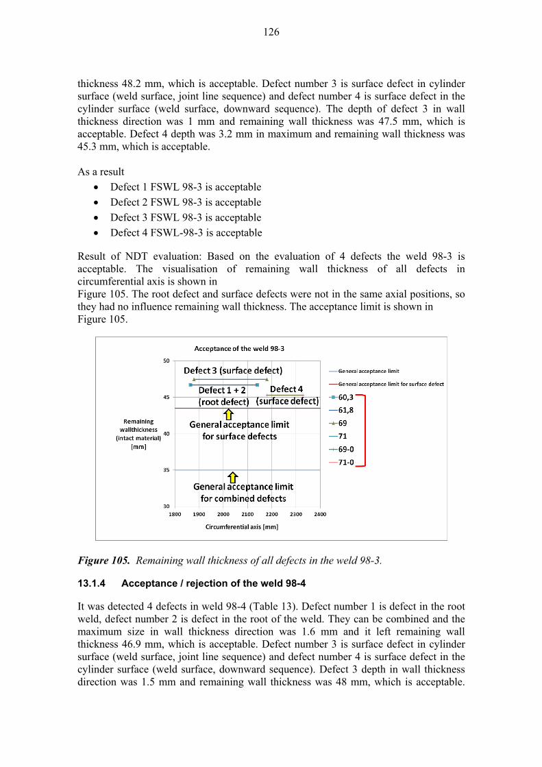
126
thickness 48.2 mm, which is acceptable. Defect number 3 is surface defect in cylinder surface (weld surface, joint line sequence) and defect number 4 is surface defect in the cylinder surface (weld surface, downward sequence). The depth of defect 3 in wall thickness direction was 1 mm and remaining wall thickness was 47.5 mm, which is acceptable. Defect 4 depth was 3.2 mm in maximum and remaining wall thickness was 45.3 mm, which is acceptable. As a result
Defect 1 FSWL 98-3 is acceptable
Defect 2 FSWL 98-3 is acceptable
Defect 3 FSWL 98-3 is acceptable
Defect 4 FSWL-98-3 is acceptable
Result of NDT evaluation: Based on the evaluation of 4 defects the weld 98-3 is acceptable. The visualisation of remaining wall thickness of all defects in circumferential axis is shown in Figure 105. The root defect and surface defects were not in the same axial positions, so they had no influence remaining wall thickness. The acceptance limit is shown in Figure 105.
Figure 105. Remaining wall thickness of all defects in the weld 98-3.
13.1.4 Acceptance / rejection of the weld 98-4
It was detected 4 defects in weld 98-4 (Table 13). Defect number 1 is defect in the root weld, defect number 2 is defect in the root of the weld. They can be combined and the maximum size in wall thickness direction was 1.6 mm and it left remaining wall thickness 46.9 mm, which is acceptable. Defect number 3 is surface defect in cylinder surface (weld surface, joint line sequence) and defect number 4 is surface defect in the cylinder surface (weld surface, downward sequence). Defect 3 depth in wall thickness direction was 1.5 mm and remaining wall thickness was 48 mm, which is acceptable.
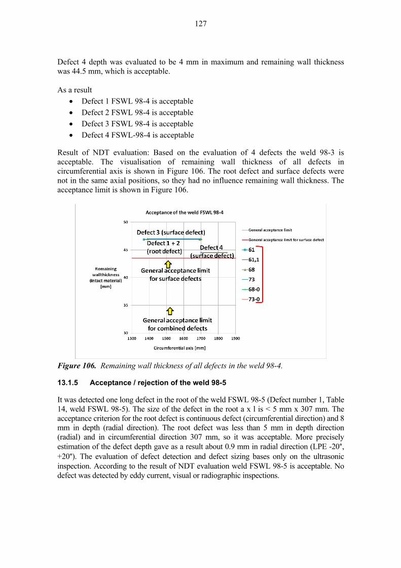
127
Defect 4 depth was evaluated to be 4 mm in maximum and remaining wall thickness was 44.5 mm, which is acceptable. As a result
Defect 1 FSWL 98-4 is acceptable
Defect 2 FSWL 98-4 is acceptable
Defect 3 FSWL 98-4 is acceptable
Defect 4 FSWL-98-4 is acceptable
Result of NDT evaluation: Based on the evaluation of 4 defects the weld 98-3 is acceptable. The visualisation of remaining wall thickness of all defects in circumferential axis is shown in Figure 106. The root defect and surface defects were not in the same axial positions, so they had no influence remaining wall thickness. The acceptance limit is shown in Figure 106.
Figure 106. Remaining wall thickness of all defects in the weld 98-4.
13.1.5 Acceptance / rejection of the weld 98-5
It was detected one long defect in the root of the weld FSWL 98-5 (Defect number 1, Table 14, weld FSWL 98-5). The size of the defect in the root a x l is < 5 mm x 307 mm. The acceptance criterion for the root defect is continuous defect (circumferential direction) and 8 mm in depth (radial direction). The root defect was less than 5 mm in depth direction (radial) and in circumferential direction 307 mm, so it was acceptable. More precisely estimation of the defect depth gave as a result about 0.9 mm in radial direction (LPE -20°, +20°). The evaluation of defect detection and defect sizing bases only on the ultrasonic inspection. According to the result of NDT evaluation weld FSWL 98-5 is acceptable. No defect was detected by eddy current, visual or radiographic inspections.

128
13.1.6 Acceptance / rejection of the weld 98-6
It was detected one long defect in the root of the weld FSWL 98-6 (Defect number 1, Table 15, weld FSWL 98-6). The size of the defect in the root a x l is < 5 mm x 230 mm. The acceptance criterion for the root defect is continuous defect (circumferential direction) and 8 mm in depth (radial direction). The root defect was less than 5 mm in depth direction (radial) and in circumferential direction 230 mm, so it was acceptable. More precisely estimation of depth was not possible. The evaluation of defect detection and defect sizing bases only on the ultrasonic inspection. According to the result of NDT evaluation weld FSWL 98-6 is acceptable. No defect was detected by eddy current, visual or radiographic inspections.
13.1.7 Acceptance / rejection of the weld 98-7
In the weld FSWL 98-7 was detected 2 root defects (Defect 1 and 2 Table 16, weld FSWL 98-7). Defect 1 was determined to be less than 5 mm in depth (radial direction) and its length 300 mm. Defect 2 was correspondingly less than 5 mm in depth (radial direction) and its length was 104 mm. The acceptance criterion for the root defect is continuous defect (circumferential direction) and 8 mm in depth (radial direction). Defect 1 could be sized more precisely and the depth was determined to be 0.7 mm in radial direction. Defect 2 could not be sized more accurately. Still both defects were acceptable according to ultrasonic evaluation. According to the result of NDT evaluation weld FSWL 98-7 is acceptable. No defect was detected by eddy current, visual or radiographic inspections.
13.2 Acceptance / rejection of weld FSWL 100
13.2.1 Acceptance / rejection of the weld 100-1
It was detected one long defect in the root of the weld FSWL 100-1 (Defect number 1, Table 17, weld FSWL 100-1). The size of the defect in the root a x l is < 5 mm x 148 mm. The acceptance criterion for the root defect is continuous defect (circumferential direction) and 8 mm in depth (radial direction). The root defect was less than 5 mm in depth direction (radial) and in circumferential direction 148 mm, so it was acceptable. More precisely estimation of depth was not possible. The evaluation of defect detection and defect sizing bases only on the ultrasonic inspection. According to the result of NDT evaluation weld FSWL 100-1 is acceptable. No defect was detected by eddy current, visual or radiographic inspections.
13.2.2 Acceptance / rejection of the weld 100-2
It was detected one long defect in the root of the weld FSWL 100-2 (Defect 1, Table 18, weld FSWL 100-2). The size of the defect in the root a x l is < 5 mm x 251 mm. The acceptance criterion for the root defect is continuous defect (circumferential direction) and 8 mm in depth (radial direction). The root defect was less than 5 mm in depth direction (radial) and in circumferential direction 251 mm, so it was acceptable. More precisely estimation of depth was not possible. The evaluation of defect detection and defect sizing bases only on the ultrasonic inspection. According to the result of NDT evaluation weld FSWL 100-1 is acceptable. No defect was detected by eddy current, visual or radiographic inspections.
129
13.2.3 Acceptance / rejection of the weld 100-3
It was detected one long defect in the root of the weld FSWL 100-3 (Defect 1, Table 19, weld FSWL 100-3). The size of the defect in the root a x l is < 5 mm x 307 mm. The acceptance criterion for the root defect is continuous defect (circumferential direction) and 8 mm in depth (radial direction). The root defect was less than 5 mm in depth direction (radial) and in circumferential direction 307 mm, so it was acceptable. Defect 1 could be sized more precisely and the depth was determined to be 2.6 mm in radial direction. The evaluation of defect detection and defect sizing bases only on the ultrasonic inspection. According to the result of NDT evaluation weld FSWL 100-3 is acceptable. No defect was detected by eddy current, visual or radiographic inspections.
13.2.4 Acceptance / rejection of the weld 100-4
It was detected one long defect in the root of the weld FSWL 100-4 (Defect 1, Table 20, weld FSWL 100-4). The size of the defect in the root a x l is < 5 mm x 320 mm. The acceptance criterion for the root defect is continuous defect (circumferential direction) and 8 mm in depth (radial direction). The root defect was less than 5 mm in depth direction (radial) and in circumferential direction 320 mm, so it was acceptable. Defect 1 could be sized more precisely and the depth was determined to be 3.2 mm in radial direction. The evaluation of defect detection and defect sizing bases only on the ultrasonic inspection. According to the result of NDT evaluation weld FSWL 100-4 is acceptable. No defect was detected by eddy current, visual or radiographic inspections.
13.2.5 Acceptance / rejection of the weld 100-5
It was detected one long defect in the root of the weld FSWL 100-5 (Defect 1, Table 21, weld FSWL 100-5). The size of the defect in the root a x l is < 5 mm x 301 mm. The acceptance criterion for the root defect is continuous defect (circumferential direction) and 8 mm in depth (radial direction). The root defect was less than 5 mm in depth direction (radial) and in circumferential direction 301 mm, so it was acceptable. Defect 1 could be sized more precisely and the depth was determined to be 2.4 mm in radial direction. The evaluation of defect detection and defect sizing bases only on the ultrasonic inspection. According to the result of NDT evaluation weld FSWL 100-5 is acceptable. No defect was detected by eddy current, visual or radiographic inspections.
13.2.6 Acceptance / rejection of the weld 100-6
It was detected one long defect in the root of the weld FSWL 100-6 (Defect 1, Table 22, weld FSWL 100-6). The size of the defect in the root a x l is < 5 mm x 306 mm. The acceptance criterion for the root defect is continuous defect (circumferential direction) and 8 mm in depth (radial direction). The root defect was less than 5 mm in depth direction (radial) and in circumferential direction 306 mm, so it was acceptable. Defect 1 could be sized more precisely and the depth was determined to be 1.7 mm in radial direction. The evaluation of defect detection and defect sizing bases only on the ultrasonic inspection. According to the result of NDT evaluation weld FSWL 100-6 is acceptable. No defect was detected by eddy current, visual or radiographic inspections.
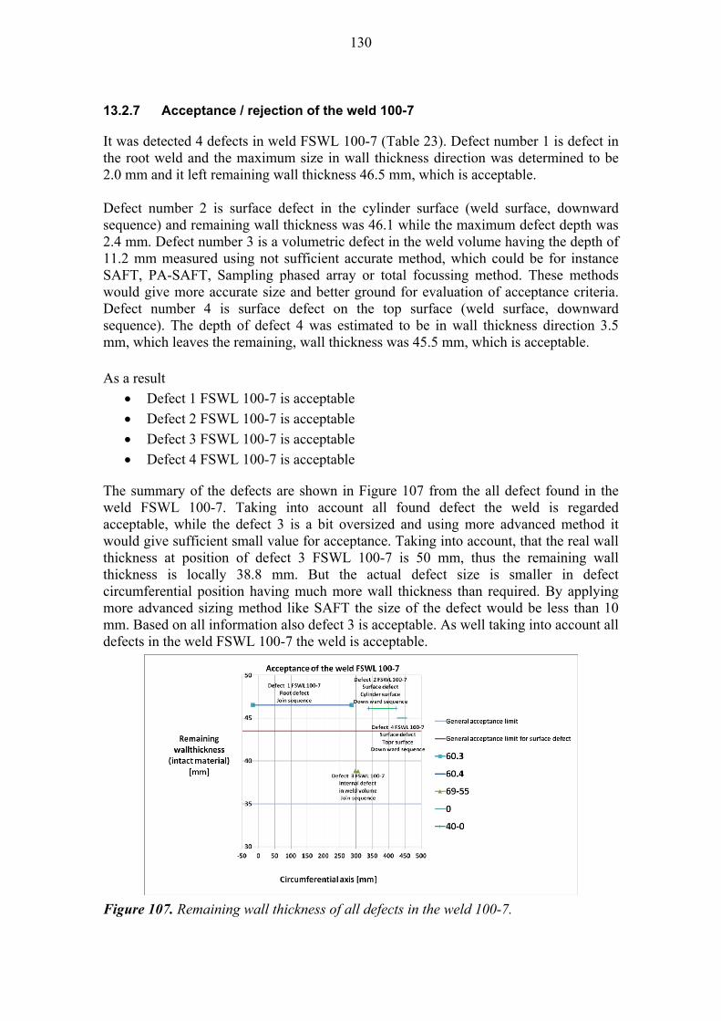
130
13.2.7 Acceptance / rejection of the weld 100-7
It was detected 4 defects in weld FSWL 100-7 (Table 23). Defect number 1 is defect in the root weld and the maximum size in wall thickness direction was determined to be 2.0 mm and it left remaining wall thickness 46.5 mm, which is acceptable. Defect number 2 is surface defect in the cylinder surface (weld surface, downward sequence) and remaining wall thickness was 46.1 while the maximum defect depth was 2.4 mm. Defect number 3 is a volumetric defect in the weld volume having the depth of 11.2 mm measured using not sufficient accurate method, which could be for instance SAFT, PA-SAFT, Sampling phased array or total focussing method. These methods would give more accurate size and better ground for evaluation of acceptance criteria. Defect number 4 is surface defect on the top surface (weld surface, downward sequence). The depth of defect 4 was estimated to be in wall thickness direction 3.5 mm, which leaves the remaining, wall thickness was 45.5 mm, which is acceptable. As a result
Defect 1 FSWL 100-7 is acceptable
Defect 2 FSWL 100-7 is acceptable
Defect 3 FSWL 100-7 is acceptable
Defect 4 FSWL 100-7 is acceptable
The summary of the defects are shown in Figure 107 from the all defect found in the weld FSWL 100-7. Taking into account all found defect the weld is regarded acceptable, while the defect 3 is a bit oversized and using more advanced method it would give sufficient small value for acceptance. Taking into account, that the real wall thickness at position of defect 3 FSWL 100-7 is 50 mm, thus the remaining wall thickness is locally 38.8 mm. But the actual defect size is smaller in defect circumferential position having much more wall thickness than required. By applying more advanced sizing method like SAFT the size of the defect would be less than 10 mm. Based on all information also defect 3 is acceptable. As well taking into account all defects in the weld FSWL 100-7 the weld is acceptable.
Figure 107. Remaining wall thickness of all defects in the weld 100-7.
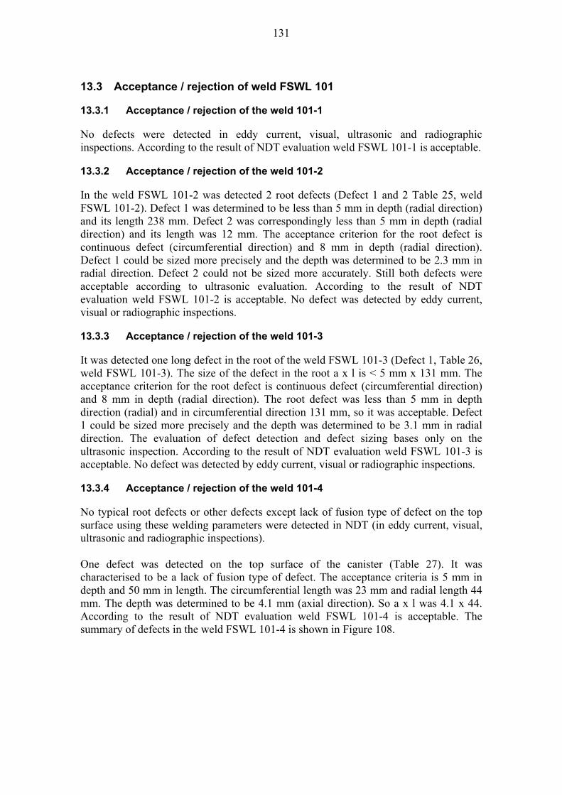
131
13.3 Acceptance / rejection of weld FSWL 101
13.3.1 Acceptance / rejection of the weld 101-1
No defects were detected in eddy current, visual, ultrasonic and radiographic inspections. According to the result of NDT evaluation weld FSWL 101-1 is acceptable.
13.3.2 Acceptance / rejection of the weld 101-2
In the weld FSWL 101-2 was detected 2 root defects (Defect 1 and 2 Table 25, weld FSWL 101-2). Defect 1 was determined to be less than 5 mm in depth (radial direction) and its length 238 mm. Defect 2 was correspondingly less than 5 mm in depth (radial direction) and its length was 12 mm. The acceptance criterion for the root defect is continuous defect (circumferential direction) and 8 mm in depth (radial direction). Defect 1 could be sized more precisely and the depth was determined to be 2.3 mm in radial direction. Defect 2 could not be sized more accurately. Still both defects were acceptable according to ultrasonic evaluation. According to the result of NDT evaluation weld FSWL 101-2 is acceptable. No defect was detected by eddy current, visual or radiographic inspections.
13.3.3 Acceptance / rejection of the weld 101-3
It was detected one long defect in the root of the weld FSWL 101-3 (Defect 1, Table 26, weld FSWL 101-3). The size of the defect in the root a x l is < 5 mm x 131 mm. The acceptance criterion for the root defect is continuous defect (circumferential direction) and 8 mm in depth (radial direction). The root defect was less than 5 mm in depth direction (radial) and in circumferential direction 131 mm, so it was acceptable. Defect 1 could be sized more precisely and the depth was determined to be 3.1 mm in radial direction. The evaluation of defect detection and defect sizing bases only on the ultrasonic inspection. According to the result of NDT evaluation weld FSWL 101-3 is acceptable. No defect was detected by eddy current, visual or radiographic inspections.
13.3.4 Acceptance / rejection of the weld 101-4
No typical root defects or other defects except lack of fusion type of defect on the top surface using these welding parameters were detected in NDT (in eddy current, visual, ultrasonic and radiographic inspections). One defect was detected on the top surface of the canister (Table 27). It was characterised to be a lack of fusion type of defect. The acceptance criteria is 5 mm in depth and 50 mm in length. The circumferential length was 23 mm and radial length 44 mm. The depth was determined to be 4.1 mm (axial direction). So a x l was 4.1 x 44. According to the result of NDT evaluation weld FSWL 101-4 is acceptable. The summary of defects in the weld FSWL 101-4 is shown in Figure 108.
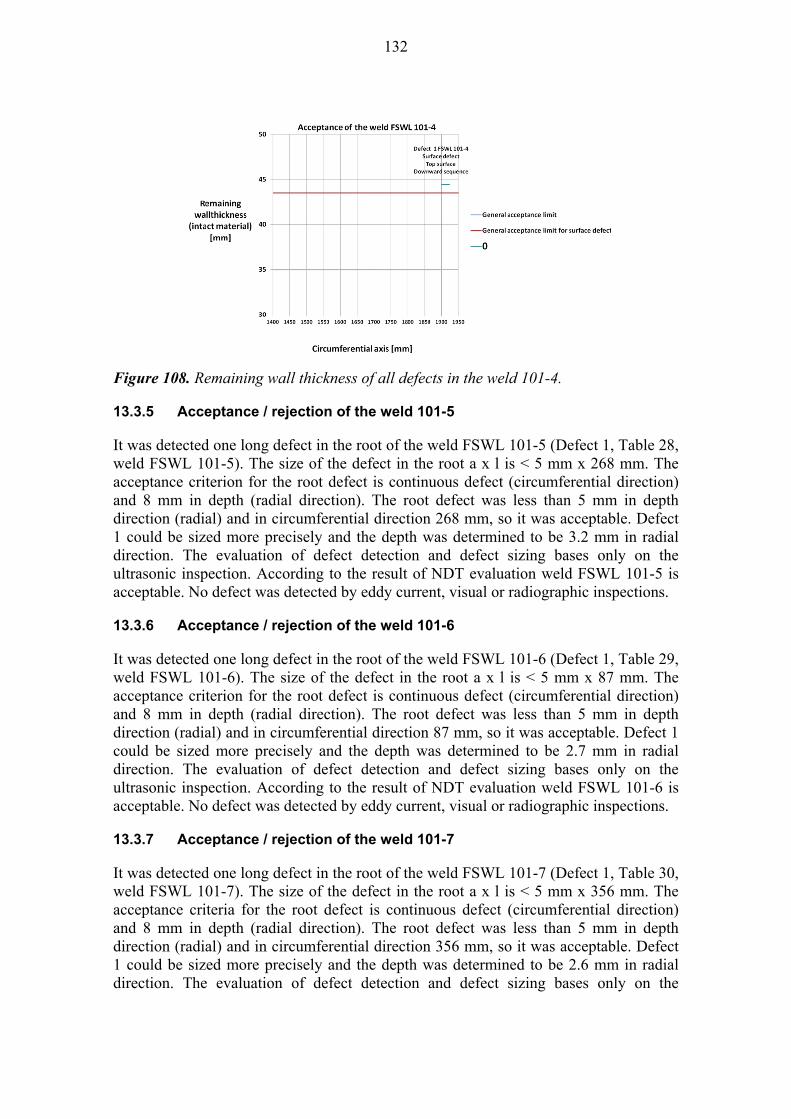
132
Figure 108. Remaining wall thickness of all defects in the weld 101-4.
13.3.5 Acceptance / rejection of the weld 101-5
It was detected one long defect in the root of the weld FSWL 101-5 (Defect 1, Table 28, weld FSWL 101-5). The size of the defect in the root a x l is < 5 mm x 268 mm. The acceptance criterion for the root defect is continuous defect (circumferential direction) and 8 mm in depth (radial direction). The root defect was less than 5 mm in depth direction (radial) and in circumferential direction 268 mm, so it was acceptable. Defect 1 could be sized more precisely and the depth was determined to be 3.2 mm in radial direction. The evaluation of defect detection and defect sizing bases only on the ultrasonic inspection. According to the result of NDT evaluation weld FSWL 101-5 is acceptable. No defect was detected by eddy current, visual or radiographic inspections.
13.3.6 Acceptance / rejection of the weld 101-6
It was detected one long defect in the root of the weld FSWL 101-6 (Defect 1, Table 29, weld FSWL 101-6). The size of the defect in the root a x l is < 5 mm x 87 mm. The acceptance criterion for the root defect is continuous defect (circumferential direction) and 8 mm in depth (radial direction). The root defect was less than 5 mm in depth direction (radial) and in circumferential direction 87 mm, so it was acceptable. Defect 1 could be sized more precisely and the depth was determined to be 2.7 mm in radial direction. The evaluation of defect detection and defect sizing bases only on the ultrasonic inspection. According to the result of NDT evaluation weld FSWL 101-6 is acceptable. No defect was detected by eddy current, visual or radiographic inspections.
13.3.7 Acceptance / rejection of the weld 101-7
It was detected one long defect in the root of the weld FSWL 101-7 (Defect 1, Table 30, weld FSWL 101-7). The size of the defect in the root a x l is < 5 mm x 356 mm. The acceptance criteria for the root defect is continuous defect (circumferential direction) and 8 mm in depth (radial direction). The root defect was less than 5 mm in depth direction (radial) and in circumferential direction 356 mm, so it was acceptable. Defect 1 could be sized more precisely and the depth was determined to be 2.6 mm in radial direction. The evaluation of defect detection and defect sizing bases only on the
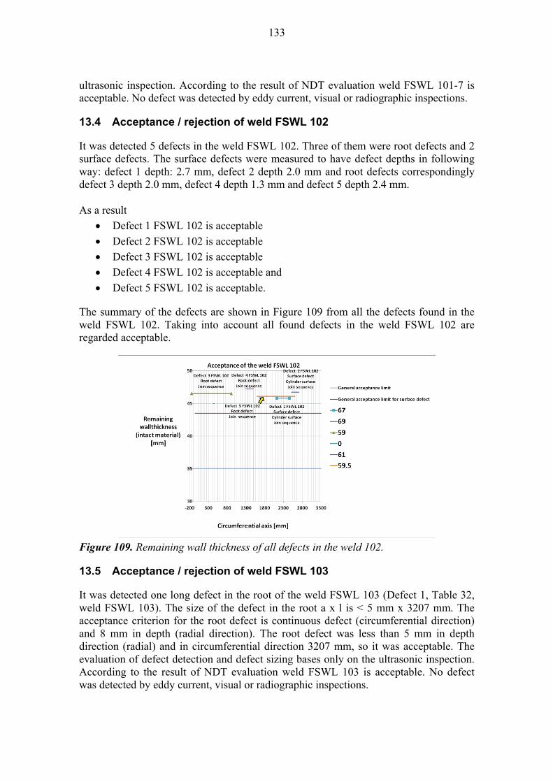
133
ultrasonic inspection. According to the result of NDT evaluation weld FSWL 101-7 is acceptable. No defect was detected by eddy current, visual or radiographic inspections.
13.4 Acceptance / rejection of weld FSWL 102
It was detected 5 defects in the weld FSWL 102. Three of them were root defects and 2 surface defects. The surface defects were measured to have defect depths in following way: defect 1 depth: 2.7 mm, defect 2 depth 2.0 mm and root defects correspondingly defect 3 depth 2.0 mm, defect 4 depth 1.3 mm and defect 5 depth 2.4 mm. As a result
Defect 1 FSWL 102 is acceptable
Defect 2 FSWL 102 is acceptable
Defect 3 FSWL 102 is acceptable
Defect 4 FSWL 102 is acceptable and
Defect 5 FSWL 102 is acceptable.
The summary of the defects are shown in Figure 109 from all the defects found in the weld FSWL 102. Taking into account all found defects in the weld FSWL 102 are regarded acceptable.
Figure 109. Remaining wall thickness of all defects in the weld 102.
13.5 Acceptance / rejection of weld FSWL 103
It was detected one long defect in the root of the weld FSWL 103 (Defect 1, Table 32, weld FSWL 103). The size of the defect in the root a x l is < 5 mm x 3207 mm. The acceptance criterion for the root defect is continuous defect (circumferential direction) and 8 mm in depth (radial direction). The root defect was less than 5 mm in depth direction (radial) and in circumferential direction 3207 mm, so it was acceptable. The evaluation of defect detection and defect sizing bases only on the ultrasonic inspection. According to the result of NDT evaluation weld FSWL 103 is acceptable. No defect was detected by eddy current, visual or radiographic inspections.
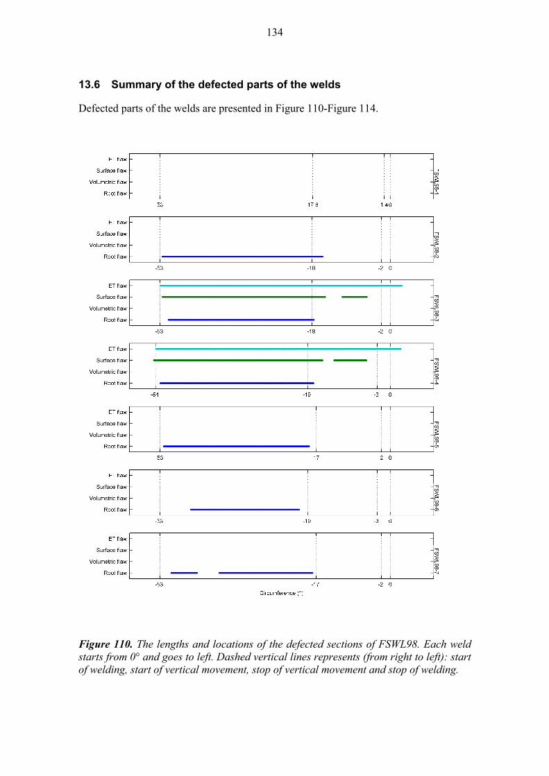
134
13.6 Summary of the defected parts of the welds
Defected parts of the welds are presented in Figure 110-Figure 114.
Figure 110. The lengths and locations of the defected sections of FSWL98. Each weld starts from 0° and goes to left. Dashed vertical lines represents (from right to left): start of welding, start of vertical movement, stop of vertical movement and stop of welding.
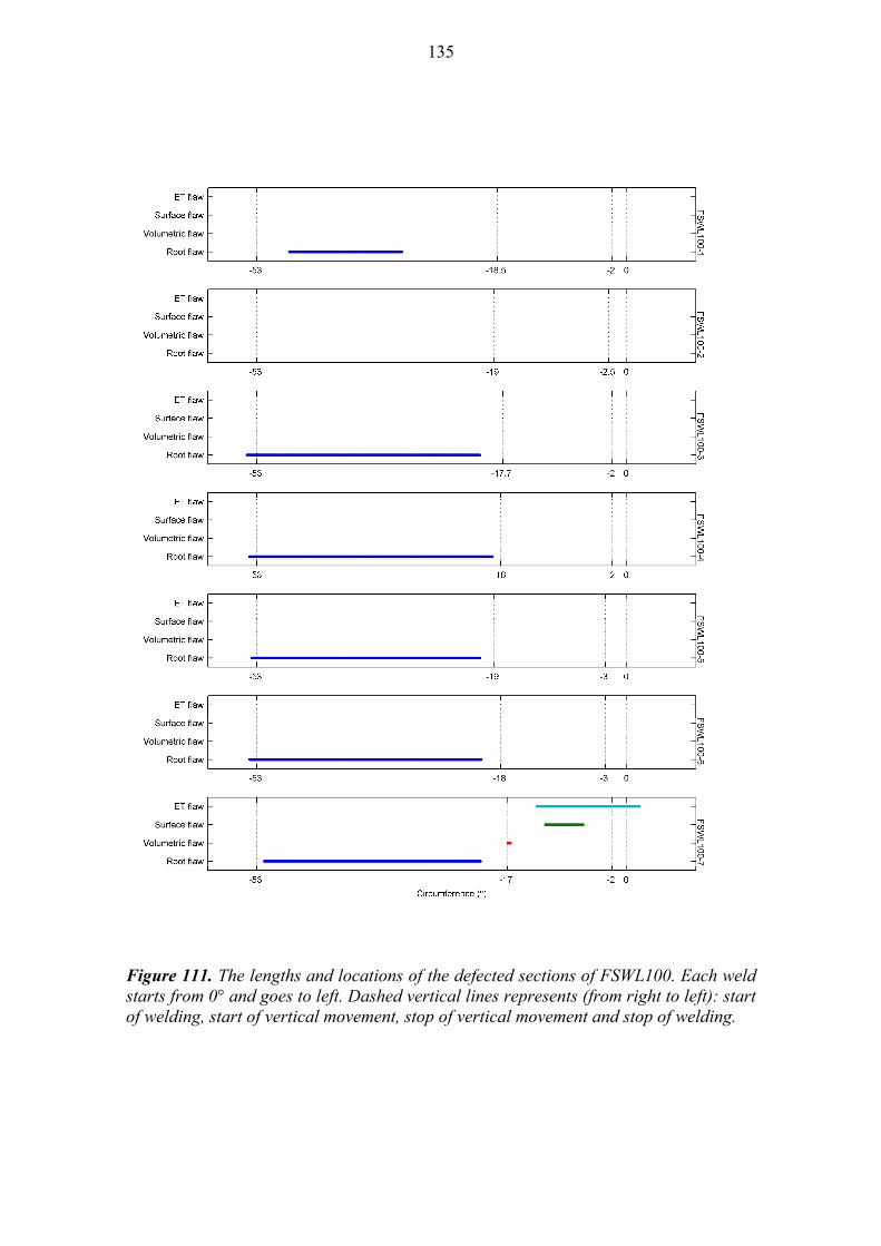
135
Figure 111. The lengths and locations of the defected sections of FSWL100. Each weld starts from 0° and goes to left. Dashed vertical lines represents (from right to left): start of welding, start of vertical movement, stop of vertical movement and stop of welding.
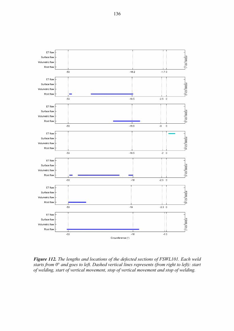
136
Figure 112. The lengths and locations of the defected sections of FSWL101. Each weld starts from 0° and goes to left. Dashed vertical lines represents (from right to left): start of welding, start of vertical movement, stop of vertical movement and stop of welding.
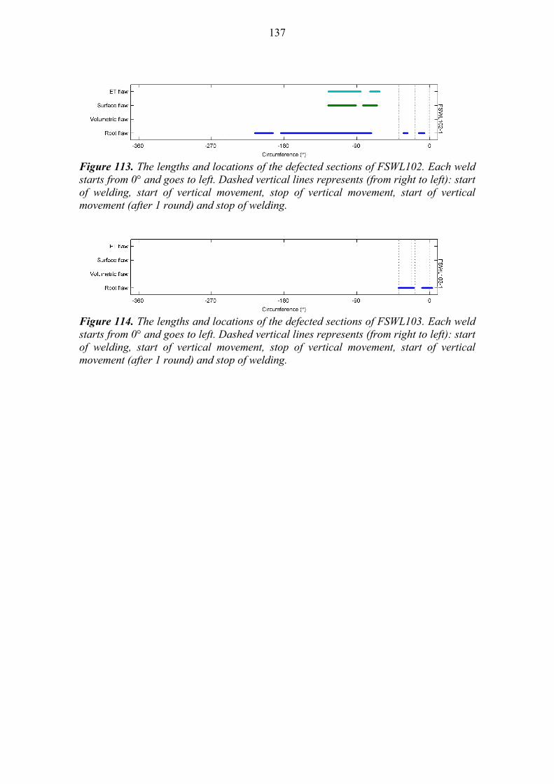
137
Figure 113. The lengths and locations of the defected sections of FSWL102. Each weld starts from 0° and goes to left. Dashed vertical lines represents (from right to left): start of welding, start of vertical movement, stop of vertical movement, start of vertical movement (after 1 round) and stop of welding.
Figure 114. The lengths and locations of the defected sections of FSWL103. Each weld starts from 0° and goes to left. Dashed vertical lines represents (from right to left): start of welding, start of vertical movement, stop of vertical movement, start of vertical movement (after 1 round) and stop of welding.

138
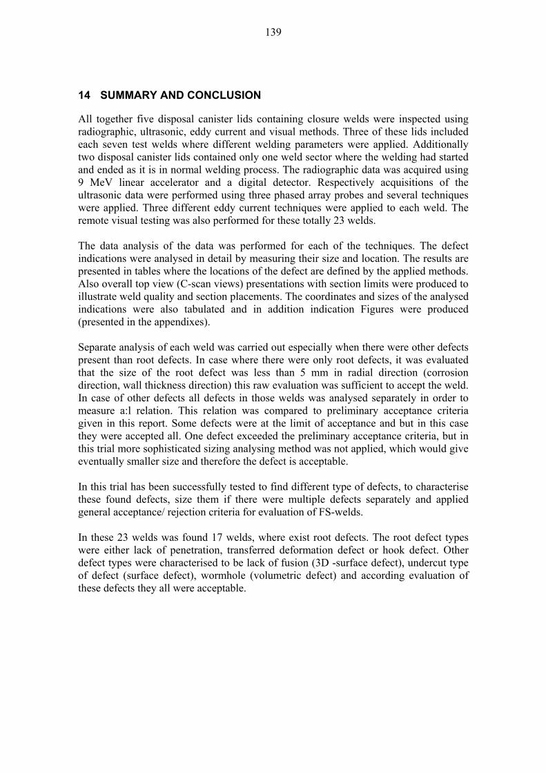
139
14 SUMMARY AND CONCLUSION
All together five disposal canister lids containing closure welds were inspected using radiographic, ultrasonic, eddy current and visual methods. Three of these lids included each seven test welds where different welding parameters were applied. Additionally two disposal canister lids contained only one weld sector where the welding had started and ended as it is in normal welding process. The radiographic data was acquired using 9 MeV linear accelerator and a digital detector. Respectively acquisitions of the ultrasonic data were performed using three phased array probes and several techniques were applied. Three different eddy current techniques were applied to each weld. The remote visual testing was also performed for these totally 23 welds. The data analysis of the data was performed for each of the techniques. The defect indications were analysed in detail by measuring their size and location. The results are presented in tables where the locations of the defect are defined by the applied methods. Also overall top view (C-scan views) presentations with section limits were produced to illustrate weld quality and section placements. The coordinates and sizes of the analysed indications were also tabulated and in addition indication Figures were produced (presented in the appendixes). Separate analysis of each weld was carried out especially when there were other defects present than root defects. In case where there were only root defects, it was evaluated that the size of the root defect was less than 5 mm in radial direction (corrosion direction, wall thickness direction) this raw evaluation was sufficient to accept the weld. In case of other defects all defects in those welds was analysed separately in order to measure a:l relation. This relation was compared to preliminary acceptance criteria given in this report. Some defects were at the limit of acceptance and but in this case they were accepted all. One defect exceeded the preliminary acceptance criteria, but in this trial more sophisticated sizing analysing method was not applied, which would give eventually smaller size and therefore the defect is acceptable. In this trial has been successfully tested to find different type of defects, to characterise these found defects, size them if there were multiple defects separately and applied general acceptance/ rejection criteria for evaluation of FS-welds. In these 23 welds was found 17 welds, where exist root defects. The root defect types were either lack of penetration, transferred deformation defect or hook defect. Other defect types were characterised to be lack of fusion (3D -surface defect), undercut type of defect (surface defect), wormhole (volumetric defect) and according evaluation of these defects they all were acceptable.

140
141
15 REFERENCES
ASME XI, 2010, Rules for inservice inspection of nuclear power plant components, Article IWA 3000, Standards for examination evaluation pp. 14 - 25. Böhm, R., 2012, internal communication. Cederqvist, L. 2011. Friction stir welding of copper canisters using power and temperature control. Doctoral thesis, Lund university, Division of machine design, Department of design science, Sweden, 139 p. Charlesworth J. P. & Temple J. A. G., 2001, Engineering application of ultrasonic Time-of Flight diffraction, Second Edition, Research Studies Press LTD, 254 p. Mishra, R-S. & Mahoney, M-W. 2007. Friction Stir Welding and Processing. Materials Park, Ohio: ASM International, 2007. ISBN: 978-0-87170-840-3. Müller, C., Elagin, M., Scharmach, M., Bellon, C., Jaenisch, G.-R., Bär, S., Redmer, B., Goebbels, J., Ewert, U., Zscherpel, U., Böhm, R., Brekow, G., Erhard, A., Heckel, T., Tessaro, U., Tscharntke D. & Ronneteg, U., 2006, Reliability of nondestructive testing (NDT) of the copper canister seal weld, SKB report R-06-08, 158p. Pitkänen, J., Salonen, J., Sandlin, S. & Ronneteg, U., 2007, Defect Detectability in EB-welded Copper Disposal Canister with 9 MeV Accelerator, 6th International Conference on NDE in Relation to Structural Integrity for Nuclear and Pressurized Components, Budapest 12th -14th October 2007, 14p. Purhonen, T., 2014, State of the art of the welding method for sealing spent nuclear fuel canister made of copper: Part 1 – FSW, Posiva working report 2014-22, p. 97. Rai, R., De, A., Bhadeshia, H.K. D.H. & Debroy, T. 2011. Review: friction stir welding tools, Science and Technology of Welding and Joining, vol 16 no 4. Raiko, H., 2012. Canister Design 2012, Posiva report 2012-13. Pitkänen J., 2010, Inspection of Bottom and Lid welds of disposal canisters, Posiva report 2010-04, 98 p. Ronneteg, U, Cederqvist, L., Ryden H., Öberg, T. and Müller, C., 2006, Reliability in sealing of canister for spent nuclear fuel, SKB Report R-06-26, 121 p. Lohwasser & Chen 2009, Friction Stir Welding, from basics to applications, Woodhead Publishing, December 436p.
142
Savolainen, K., 2004, Friction Stir Weldability of Copper Alloys. M.Sc. Thesis. Helsinki University of Technology, Laboratory of Engineering Materials, 115p + 3 appendices. Savolainen 2012, Friction Stir Welding of Copper and Microstructure and Properties of the Welds, Doctoral Dissertation 13/2012, Department of Engineering Design and Production, February, 170p. SFS-EN 583-6, 2008, Non-destructive testing, Ultrasonic examination, Time-of-flight diffraction technique as a method for detection and sizing of discontinuities 26p. SFS-EN ISO 25239-5, 2012, Friction stir welding – Aluminium – Part 5: Quality and inspection requirements. Finnish stanrdards association, 9p. SFS ISO 6520-1, 2008, Welding and allied processes. Classification of geometric imperfections in metallic materials: Part 1: Fusion Welding 49p. SKB, 2006, Kapsel för använt kärnbränsle, Tillverkning av kapselkomponenter, SKB Report R-06-03, 2006, 67p. Yamada, H., Yano, Y. & Udagawa T., 2004, Development of the phased array system for angle beam testing, Nippon Steel Technical report N089 January 2004, pp. 28-32.
143
APPENDIXES APPENDIX 1 : WELD PENETRATION MEASUREMENTS ....................................... 145APPENDIX 2 : CORNER AMPLITUDE MEASUREMENT ......................................... 147 APPENDIX 3 : WELD ATTENUATION ....................................................................... 149 APPENDIX 4 : WCL MEASUREMENTS .....................................................................151APPENDIX 5 : EDDY CURRENT INDICATIONS ....................................................... 155

144
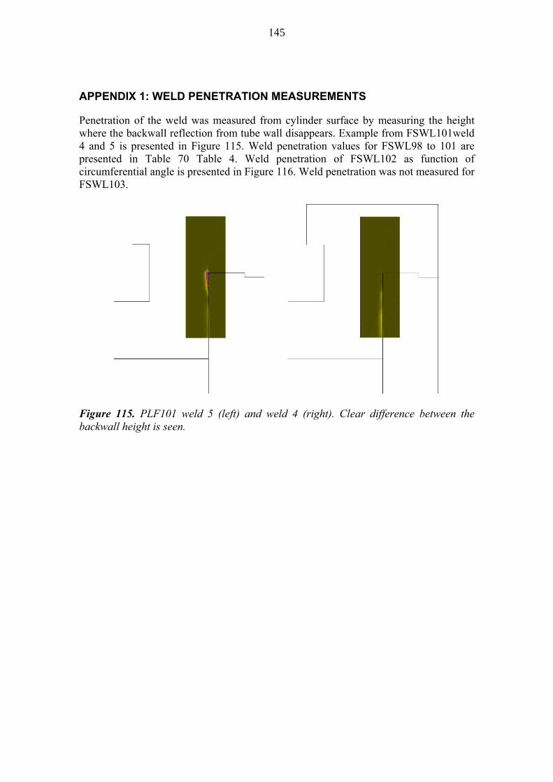
145
APPENDIX 1: WELD PENETRATION MEASUREMENTS
Penetration of the weld was measured from cylinder surface by measuring the height where the backwall reflection from tube wall disappears. Example from FSWL101weld 4 and 5 is presented in Figure 115. Weld penetration values for FSWL98 to 101 are presented in Table 70 Table 4. Weld penetration of FSWL102 as function of circumferential angle is presented in Figure 116. Weld penetration was not measured for FSWL103.
Figure 115. PLF101 weld 5 (left) and weld 4 (right). Clear difference between the backwall height is seen.
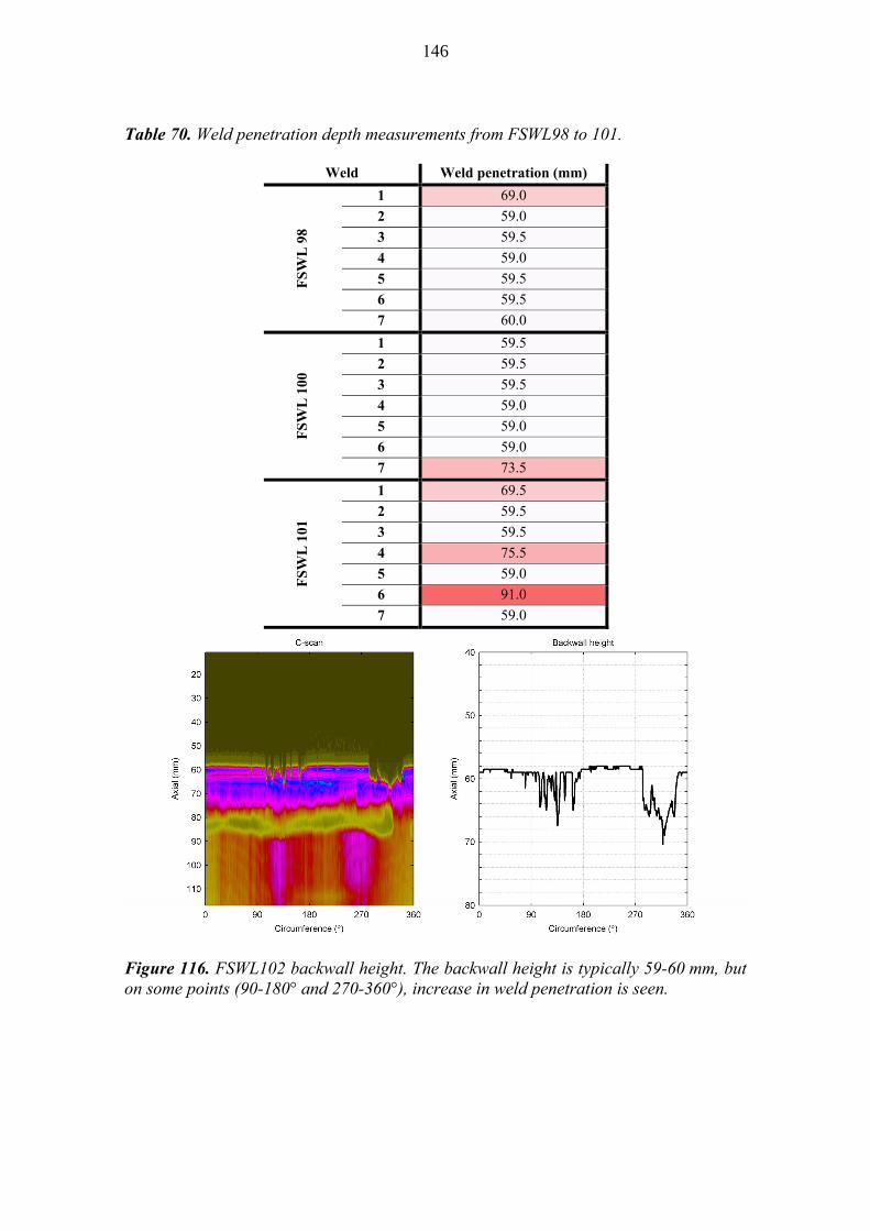
146
Table 70. Weld penetration depth measurements from FSWL98 to 101.
Weld Weld penetration (mm)
FS
WL
98
1 69.0
2 59.0
3 59.5
4 59.0
5 59.5
6 59.5
7 60.0 F
SW
L 1
00
1 59.5
2 59.5
3 59.5
4 59.0
5 59.0
6 59.0
7 73.5
FS
WL
101
1 69.5
2 59.5
3 59.5
4 75.5
5 59.0
6 91.0
7 59.0
Figure 116. FSWL102 backwall height. The backwall height is typically 59-60 mm, but on some points (90-180° and 270-360°), increase in weld penetration is seen.
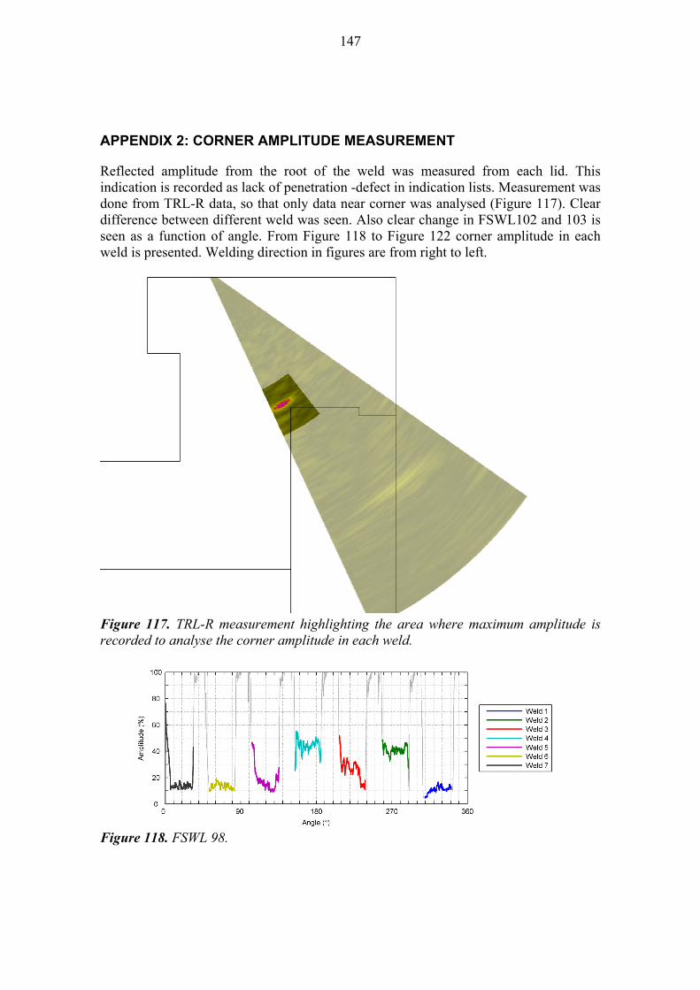
147
APPENDIX 2: CORNER AMPLITUDE MEASUREMENT
Reflected amplitude from the root of the weld was measured from each lid. This indication is recorded as lack of penetration -defect in indication lists. Measurement was done from TRL-R data, so that only data near corner was analysed (Figure 117). Clear difference between different weld was seen. Also clear change in FSWL102 and 103 is seen as a function of angle. From Figure 118 to Figure 122 corner amplitude in each weld is presented. Welding direction in figures are from right to left.
Figure 117. TRL-R measurement highlighting the area where maximum amplitude is recorded to analyse the corner amplitude in each weld.
Figure 118. FSWL 98.
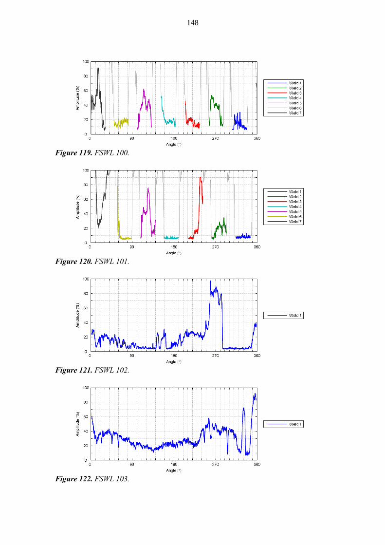
148
Figure 119. FSWL 100.
Figure 120. FSWL 101.
Figure 121. FSWL 102.
Figure 122. FSWL 103.
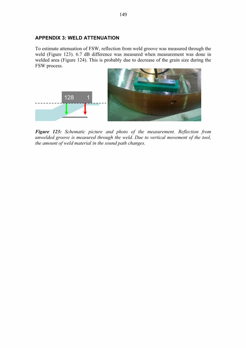
149
APPENDIX 3: WELD ATTENUATION
To estimate attenuation of FSW, reflection from weld groove was measured through the weld (Figure 123). 6.7 dB difference was measured when measurement was done in welded area (Figure 124). This is probably due to decrease of the grain size during the FSW process.
128 1
Figure 123: Schematic picture and photo of the measurement. Reflection from unwelded groove is measured through the weld. Due to vertical movement of the tool, the amount of weld material in the sound path changes.
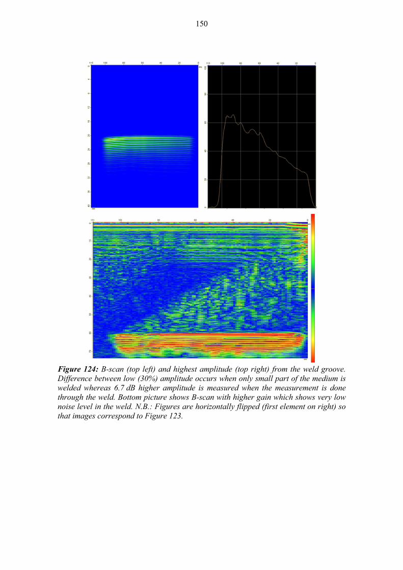
150
Figure 124: B-scan (top left) and highest amplitude (top right) from the weld groove. Difference between low (30%) amplitude occurs when only small part of the medium is welded whereas 6.7 dB higher amplitude is measured when the measurement is done through the weld. Bottom picture shows B-scan with higher gain which shows very low noise level in the weld. N.B.: Figures are horizontally flipped (first element on right) so that images correspond to Figure 123.
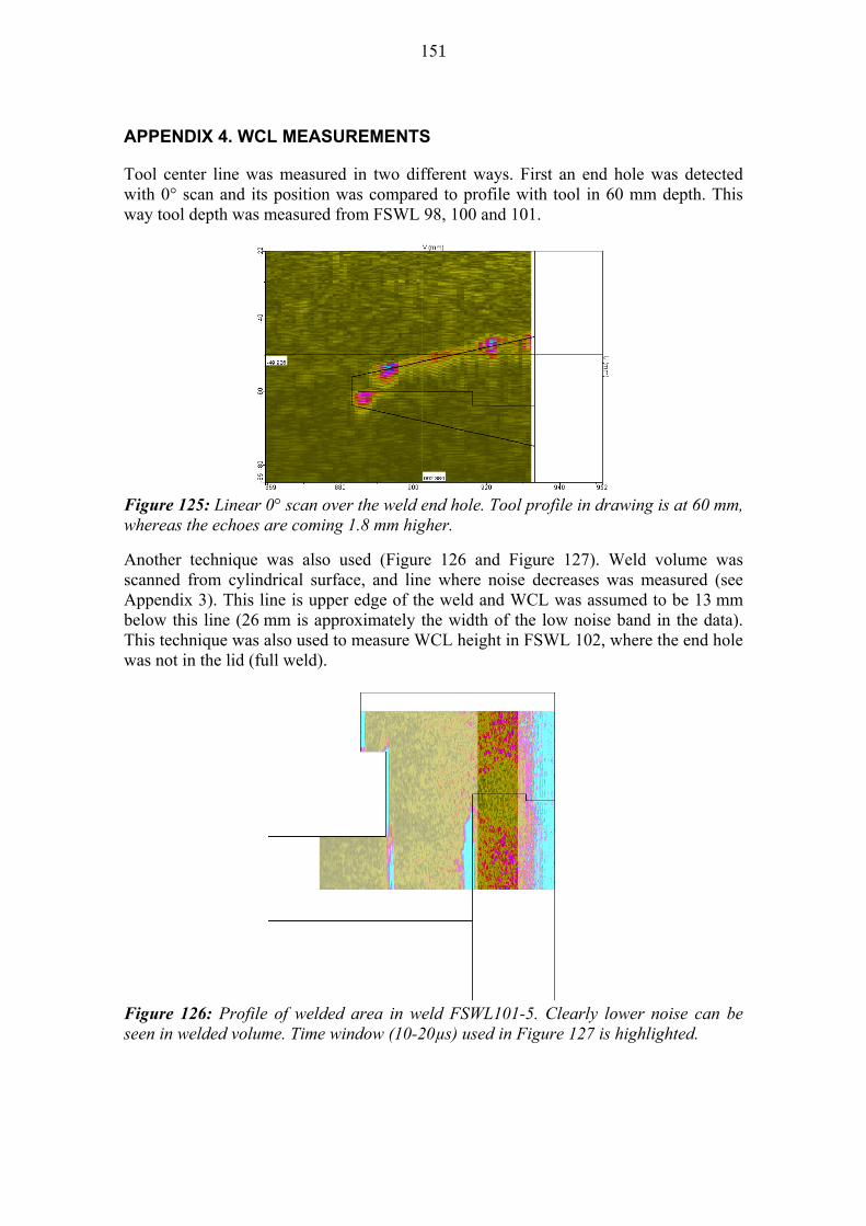
151
APPENDIX 4. WCL MEASUREMENTS
Tool center line was measured in two different ways. First an end hole was detected with 0° scan and its position was compared to profile with tool in 60 mm depth. This way tool depth was measured from FSWL 98, 100 and 101.
Figure 125: Linear 0° scan over the weld end hole. Tool profile in drawing is at 60 mm, whereas the echoes are coming 1.8 mm higher.
Another technique was also used (Figure 126 and Figure 127). Weld volume was scanned from cylindrical surface, and line where noise decreases was measured (see Appendix 3). This line is upper edge of the weld and WCL was assumed to be 13 mm below this line (26 mm is approximately the width of the low noise band in the data). This technique was also used to measure WCL height in FSWL 102, where the end hole was not in the lid (full weld).
Figure 126: Profile of welded area in weld FSWL101-5. Clearly lower noise can be seen in welded volume. Time window (10-20µs) used in Figure 127 is highlighted.
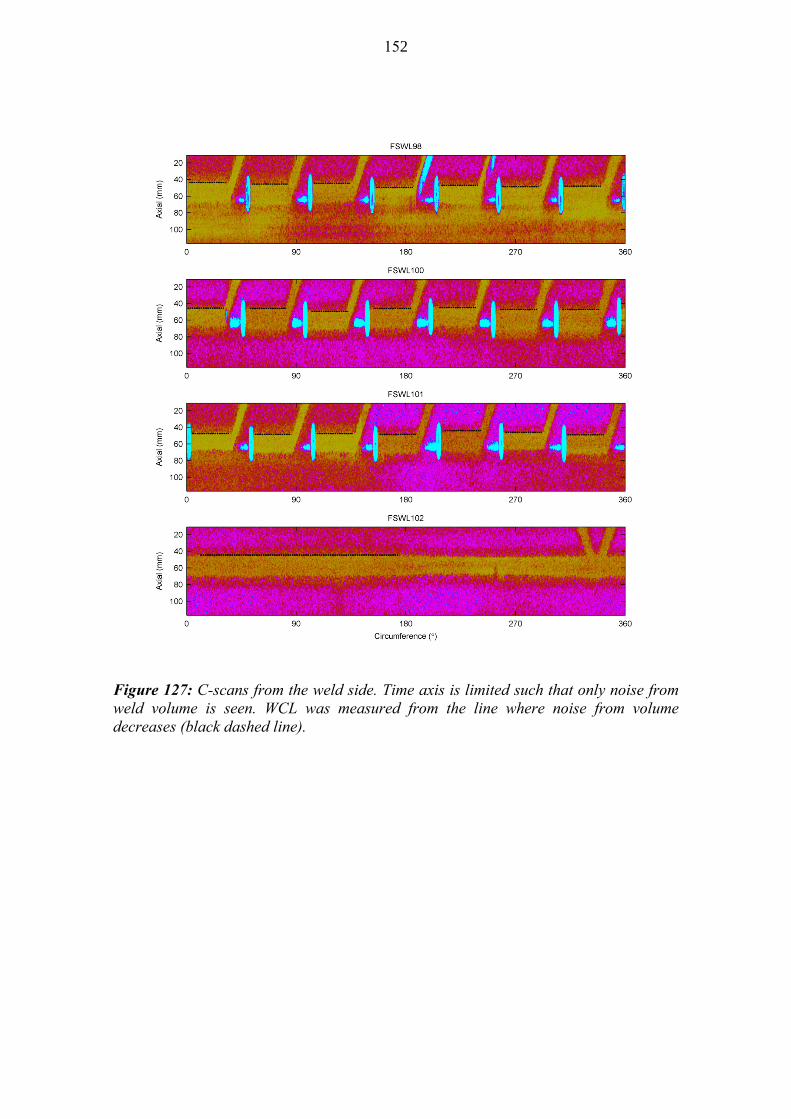
152
Figure 127: C-scans from the weld side. Time axis is limited such that only noise from weld volume is seen. WCL was measured from the line where noise from volume decreases (black dashed line).
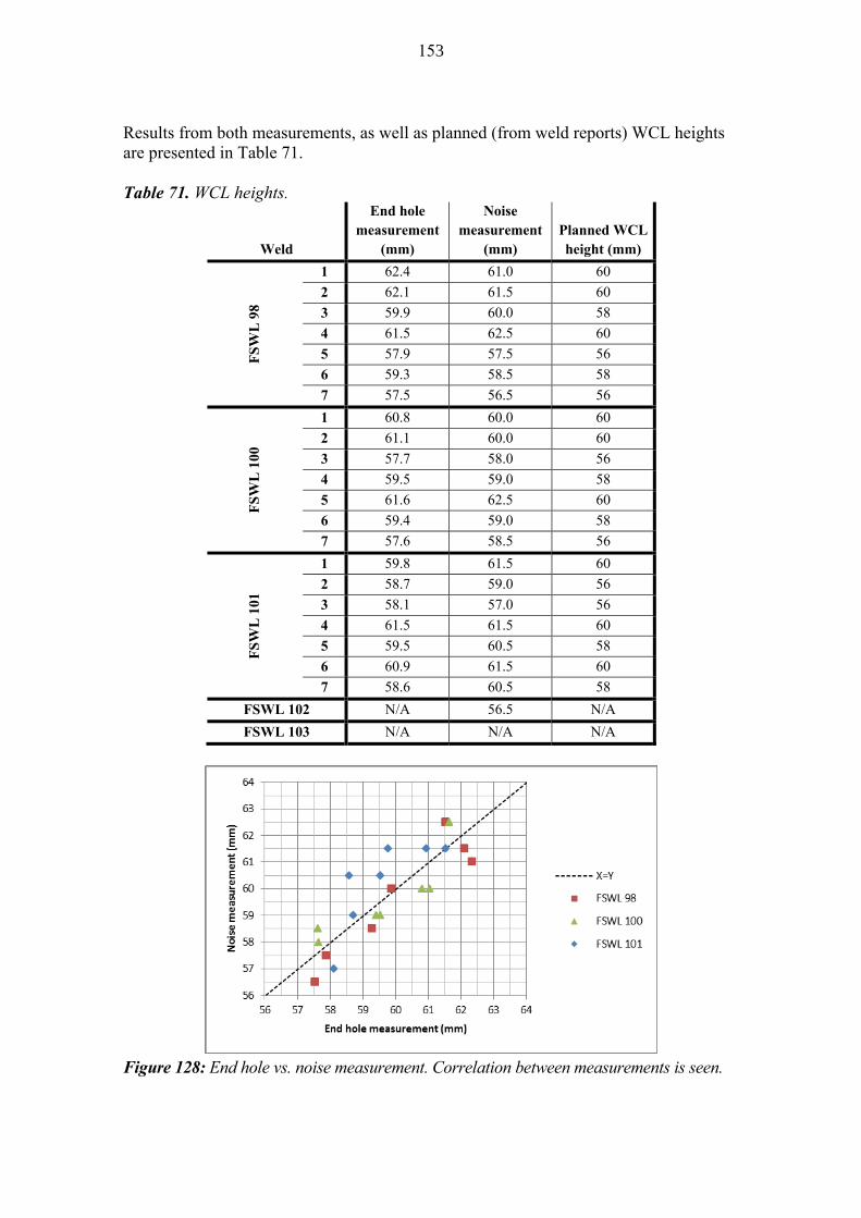
153
Results from both measurements, as well as planned (from weld reports) WCL heights are presented in Table 71. Table 71. WCL heights.
Weld
End hole measurement
(mm)
Noise measurement
(mm) Planned WCL height (mm)
FS
WL
98
1 62.4 61.0 60
2 62.1 61.5 60
3 59.9 60.0 58
4 61.5 62.5 60
5 57.9 57.5 56
6 59.3 58.5 58
7 57.5 56.5 56
FS
WL
100
1 60.8 60.0 60
2 61.1 60.0 60
3 57.7 58.0 56
4 59.5 59.0 58
5 61.6 62.5 60
6 59.4 59.0 58
7 57.6 58.5 56
FS
WL
101
1 59.8 61.5 60
2 58.7 59.0 56
3 58.1 57.0 56
4 61.5 61.5 60
5 59.5 60.5 58
6 60.9 61.5 60
7 58.6 60.5 58
FSWL 102 N/A 56.5 N/A
FSWL 103 N/A N/A N/A
Figure 128: End hole vs. noise measurement. Correlation between measurements is seen.

154
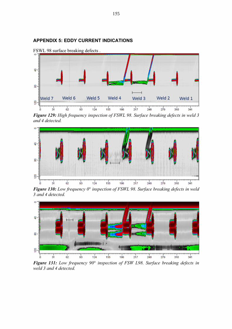
155
APPENDIX 5: EDDY CURRENT INDICATIONS
FSWL 98 surface breaking defects .
Figure 129: High frequency inspection of FSWL 98. Surface breaking defects in weld 3 and 4 detected.
Figure 130: Low frequency 0° inspection of FSWL 98. Surface breaking defects in weld 3 and 4 detected.
Figure 131: Low frequency 90° inspection of FSW L98. Surface breaking defects in weld 3 and 4 detected.

156
The weld FSWL 98-3 & FSWL 98-4
Figure 132. Top surface measurements of FSWL98-3&4. Upper left: HF measurement of FSWL 98-4. Upper right: HF measurement of FSWL 98-3. Bottom left: LF0 measurement. Bottom right: LF90 measurement.
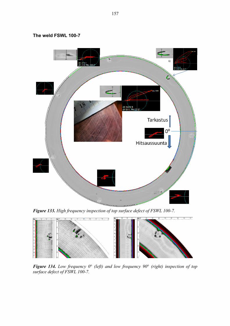
157
The weld FSWL 100-7
Figure 133. High frequency inspection of top surface defect of FSWL 100-7.
Figure 134. Low frequency 0° (left) and low frequency 90° (right) inspection of top surface defect of FSWL 100-7.

158
FSWL 100
Figure 135: High frequency inspection of FSWL 100. Surface breaking defect in weld 7 detected.
Figure 136: Low frequency 0° inspection of FSWL 100. Surface breaking defect in weld 7 detected.
Figure 137: Low frequency 90° inspection of FSWL 100. Surface breaking defect in weld 7 detected.
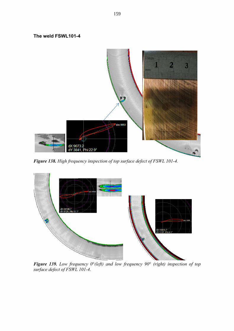
159
The weld FSWL101-4
Figure 138. High frequency inspection of top surface defect of FSWL 101-4.
Figure 139. Low frequency 0°(left) and low frequency 90° (right) inspection of top surface defect of FSWL 101-4.
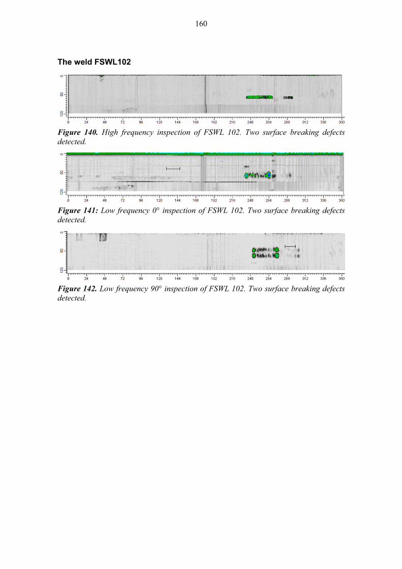
160
The weld FSWL102
Figure 140. High frequency inspection of FSWL 102. Two surface breaking defects detected.
Figure 141: Low frequency 0° inspection of FSWL 102. Two surface breaking defects detected.
Figure 142. Low frequency 90° inspection of FSWL 102. Two surface breaking defects detected.


![Non-destructive Evaluation of Friction Stir Welded Joints ... · strength of the FSW joint for AC4C Al alloy and Steel dissimilar friction stir lap joints [7]. Aluminum alloy welds](https://img.pdfslide.us/doc/110x75/5e5c511832f9297d8a597cf4/non-destructive-evaluation-of-friction-stir-welded-joints-strength-of-the-fsw.jpg)