25 October 2007 NCTM Regional Conference and Exposition, Kansas City, Missouri

Your Chance to See Original, Historical,

Classic, and Rare Mathematics Books

Richard Delaware Department of Mathematics and Statistics

University of Missouri – Kansas City

delawarer@umkc.edu Personal Web Site: http://d.faculty.umkc.edu/delawarer/ [This talk will be posted here.]

Department Web Site: http://cas.umkc.edu/math/

__________________________________________________________________________________

Thirteen books on display courtesy of the LINDA HALL LIBRARY of Science, Engineering & Technology

http://www.lindahall.org 5109 Cherry St., Kansas City, MO 64110

Bruce Bradley, Librarian for History of Science

(816) 926-8737

NOTE: Further special viewing of these and other books at Linda Hall Library Rare Book Room on: Thurs. Oct. 25, 2:00-5:00 pm, Fri. Oct. 26, 1:00-5:00 pm, & Sat. Oct. 27, 10 am – 12 noon. Images taken by Linda Hall Library; Historical notes from Bruce Bradley, and :

• Katz, Victor J., A History of Mathematics: An Introduction, 2nd Ed, 1998

2

Contents Chronological by date of first editions

__________________________________________________________________________________ PAGE 3 Euclid 1482, 1570, 1847 8 Recorde 1542 10 Bombelli 1572 13 Descartes 1637 16 Galilei 1638 19 Newton 1671, 1687 24 L’Hospital 1696 25 de Moivre 1718 29 Maclaurin 1742 31 Agnesi 1748 33 Notes from my History of Mathematics course __________________________________________________________________________________

3

Euclid, c. 300 BCE

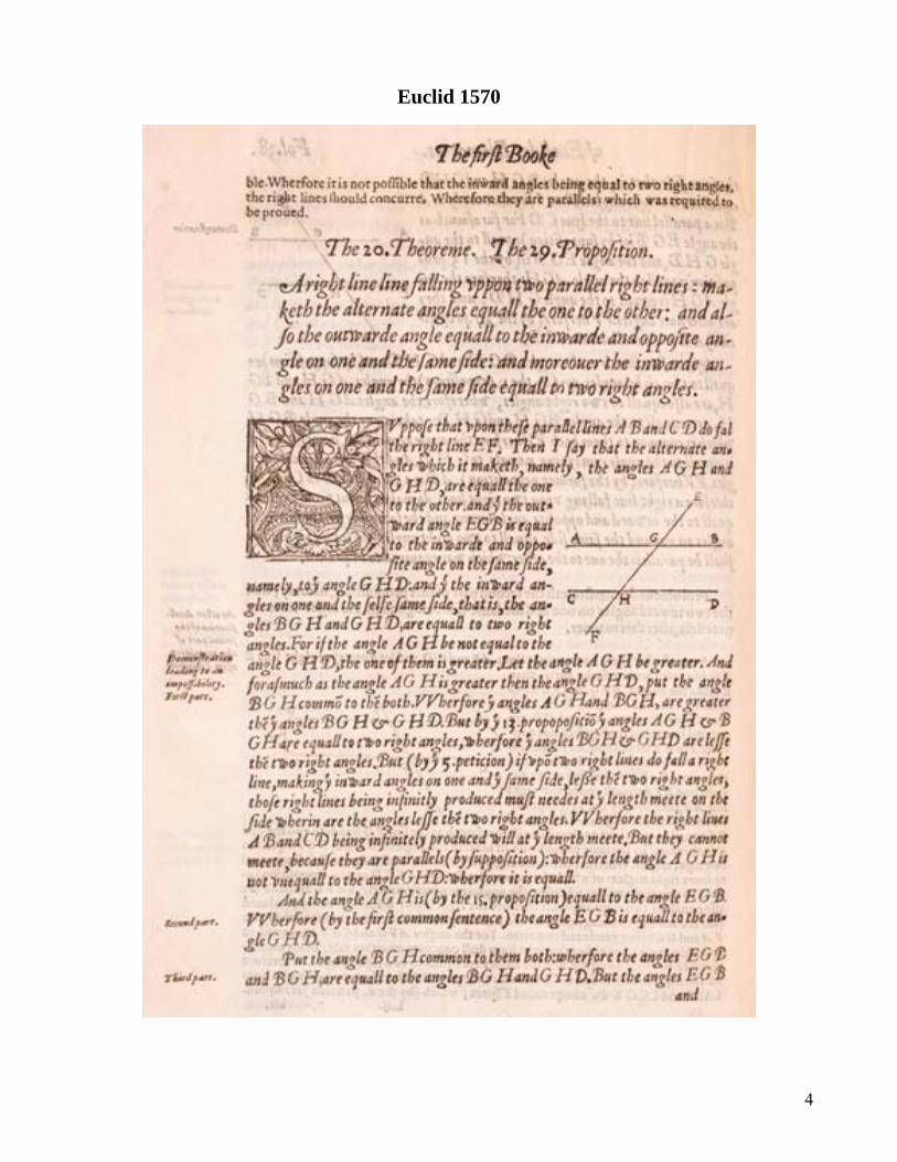
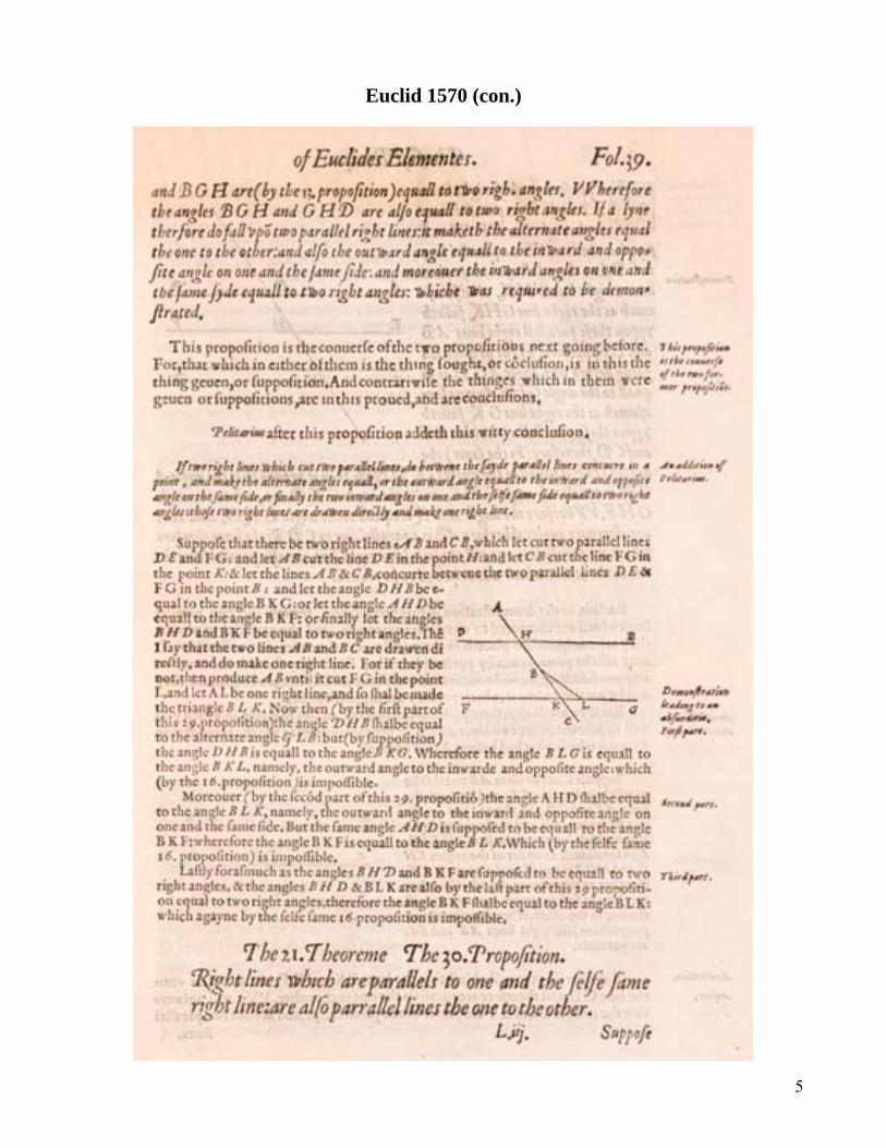
The Elements of Geometry First Printed Edition, in Latin, 1482 Elementa geometria. Venice: Erhard Ratdolt, 1482. After Gutenberg’s invention of the printing press, Euclid’s Elements of Geometry was the first mathematical work to be printed, and the first major work to be illustrated with mathematical diagrams. First English Translation, 1570 The Elements of geometrie. London: Imprinted ... by John Daye, 1570. The 1570 publication of this book, also known as the Billingsley translation, contains a preface by John Dee who also added annotations and additional theorems. This edition is especially noted for the addition of pop-ups, to illustrate problems of solid geometry as three-dimensional figures in book eleven. Euclid in Color, 1847 Byrne, Oliver, The first six books of the elements of Euclid, in which coloured diagrams and symbols are used instead of letters for the greater ease of learners. London: William Pickering [of P & Chatto], 1847. Oliver Byrne’s edition of Euclid’s Elements substituted colors for the usual letters to designate the angles and lines of geometric figures, making it one of the oddest and most beautiful mathematical books ever printed. It was also one of the most difficult to print, as the use of color wood blocks required exact registration to correctly align the pages for pass through the printing press for the different colors of ink. Byrne’s Euclid http://www.sunsite.ubc.ca/DigitalMathArchives/Euclid/byrne.html With live Java diagrams http://aleph0.clarku.edu/~djoyce/java/elements/elements.html The Visual Elements of Euclid http://www.visual-euclid.org

4

Euclid 1570

5

Euclid 1570 (con.)

6

Byrne’s Euclid 1847

7

Byrne’s Euclid 1847 (con.)

8

Robert Recorde, 1510-1558 The Ground of Artes

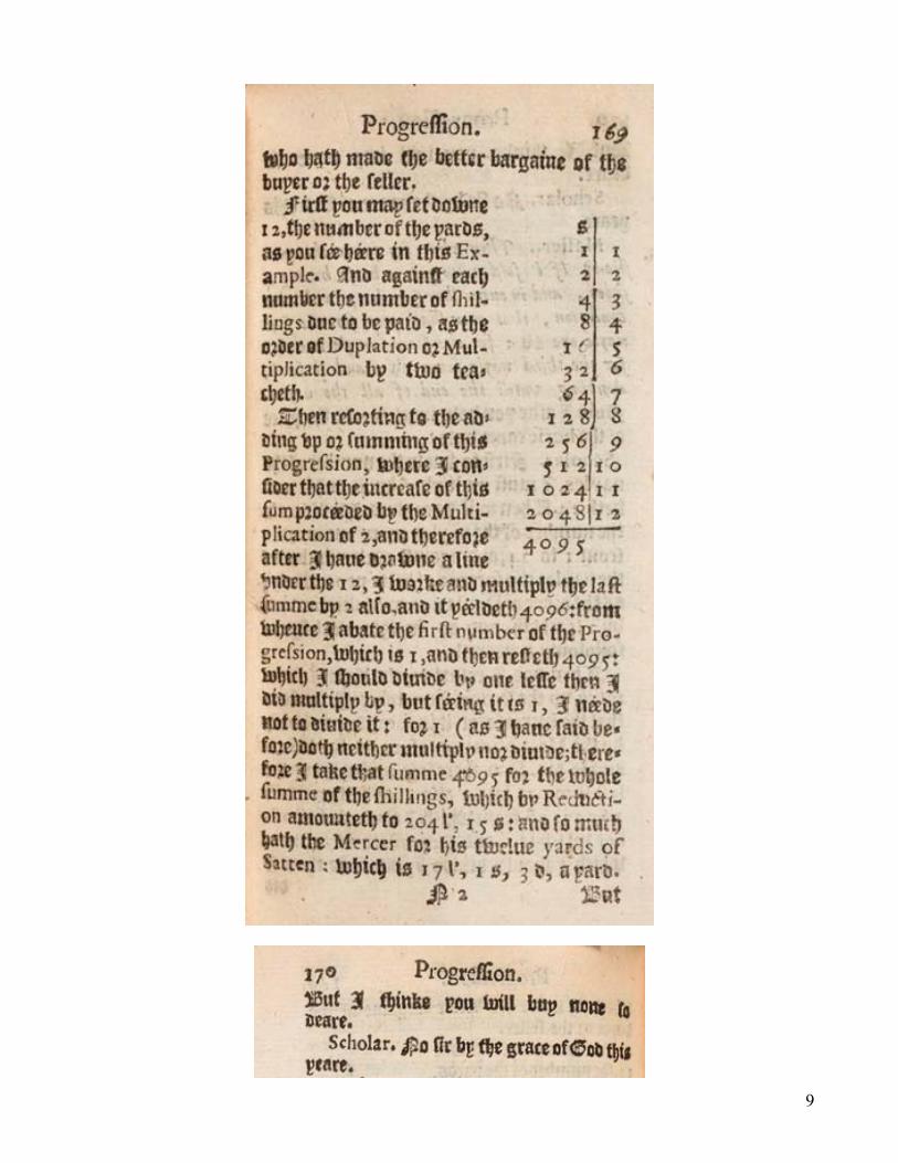
1623 (first edition 1542) Ground of arts; teaching the perfect works and practice of arithmeticke, both in whole numbers and fractions...afterwards augmented by John.. Dee, and since enlarged ... by John Mellis...[and] Robert Hartwell. London: John Beale for Roger Jackson, 1623. Record wrote several books on mathematical subjects, mainly in the form of a dialog between a master and a scholar. The Grounde of Artes first appeared in 1542 and included only a section on Arithmetic. In 1557, he published the first book on algebra in English, The Whetstone of Witte, made famous by his invention of a symbol (=) to express equality. In this 1623 edition of the Grounde of Artes (one of at least 27 early editions!), the book on algebra was included as the second part. Ironically, the equal symbol was not used by the editors, and only slowly came into common use later in the seventeenth century.

9

10

Raffaele Bombelli, 1526-1572 Algebra

1579 (original edition 1572) L'algebra opera di Rafael Bombelli da Bologna. Diuisa in tre libri. Bologna: Per Giouanni Rossi, 1579 Bombelli’s was not the first book on algebra. In 1545, Girolamo Cardano explored the subject in depth in his treatise, the Ars Magna. But Cardano’s was a difficult book, Bombelli judged, and the world needed an algebra text that would allow anyone to master the subject. So Bombelli wrote one between 1557 and 1560, finally printed in 1572, intended as a systematic and logical textbook. Only three parts (of five) were published, but it was so successful that Leibniz, who used Bombelli’s Algebra to teach himself mathematics a century later, called Bombelli the “outstanding master of the analytical art.”

11

12

13

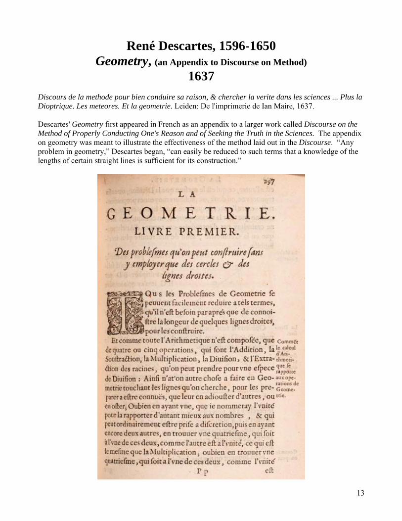
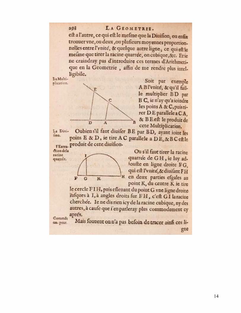
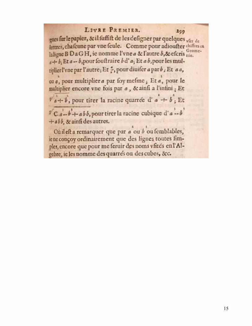
René Descartes, 1596-1650 Geometry, (an Appendix to Discourse on Method)

1637 Discours de la methode pour bien conduire sa raison, & chercher la verite dans les sciences ... Plus la Dioptrique. Les meteores. Et la geometrie. Leiden: De l'imprimerie de Ian Maire, 1637. Descartes' Geometry first appeared in French as an appendix to a larger work called Discourse on the Method of Properly Conducting One's Reason and of Seeking the Truth in the Sciences. The appendix on geometry was meant to illustrate the effectiveness of the method laid out in the Discourse. “Any problem in geometry,” Descartes began, “can easily be reduced to such terms that a knowledge of the lengths of certain straight lines is sufficient for its construction.”

14

15

16

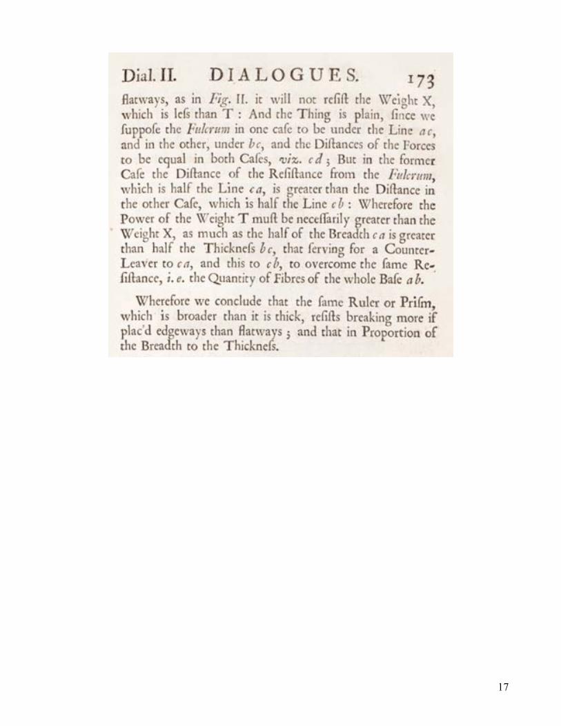
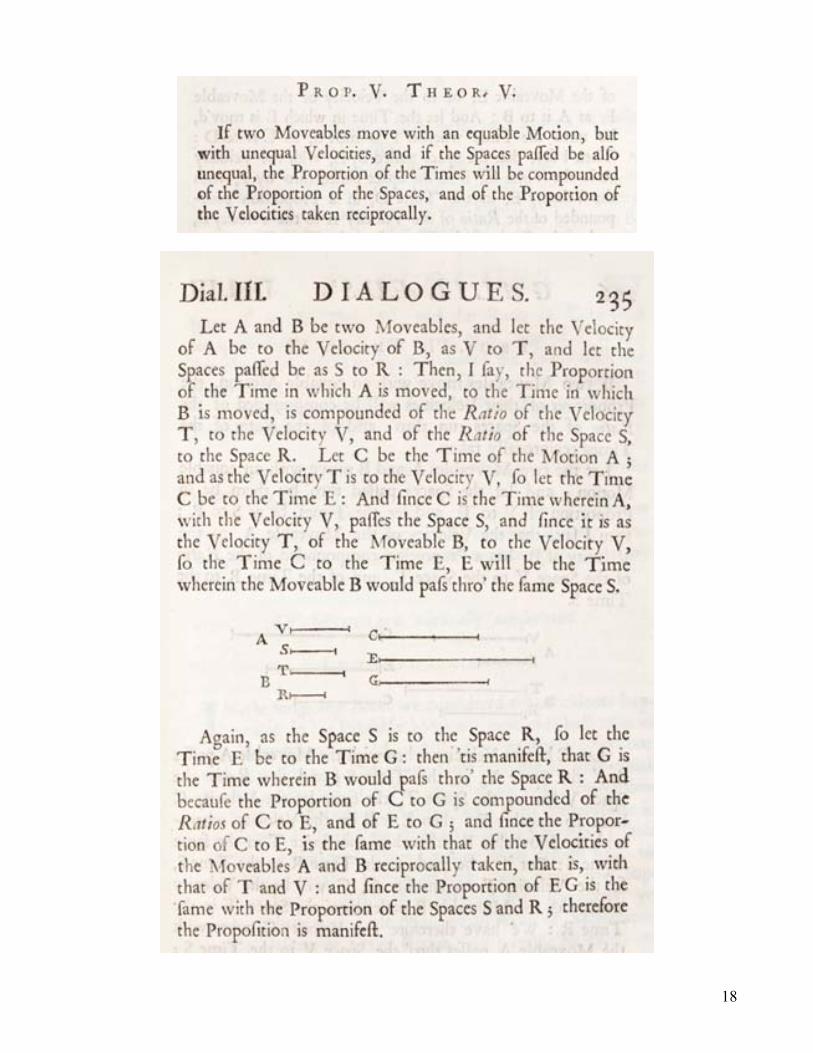
Galileo Galilei, 1564-1642 Discourses and Mathematical Demonstrations

Concerning Two New Sciences 1730 (Original edition 1638)

Mathematical discourses concerning two new sciences relating to mechanicks and local motion. London: Printed for J. Hooke, 1730.

Galileo is known for his telescopic discoveries and his controversial defense of Copernicus. But when the church forbade him from further speculation and writing about astronomy, he retreated to consider problems of mathematics and engineering. The result was this book setting forth the mathematical principles of statics (the strength of materials), and kinematics (the science of bodies in motion).

17

18

19

Isaac Newton, 1642-1727 Treatise on the Method of Series and Fluxions

1736 postumously (first edition 1671 in Latin, trans. by John Colson)

& Mathematical Principles of Natural Philosophy

third edition, Latin 1726 (first edition 1687)

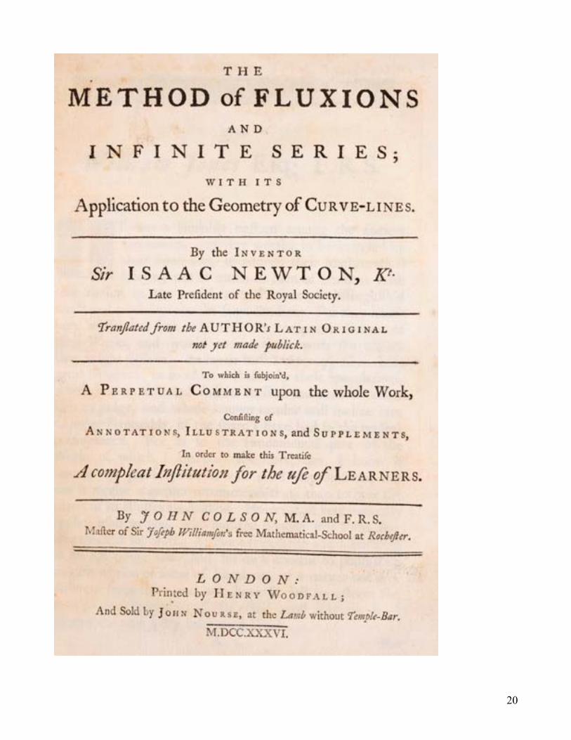
The method of fluxions and infinite series : with its application to the geometry of curve-lines. London: Printed by Henry Woodfall; and sold by John Nourse, 1736. Newton’s earliest work on the calculus, as documented in his unpublished manuscripts, came in 1665 –the same year that he took his B.A. degree. His most complete exposition on the calculus was written in 1671, in Latin, but it remained unpublished until this English translation by John Colson appeared in 1736. According to Newton, a variable was regarded as a “fluent,” and thought of as a function of time, while its rate of change with respect to time was called a “fluxion.” The basic problem this “calculus” was to investigate relations among fluents and their fluxions. Philosophiae naturalis principia mathematica. London: Apud Guil. & Joh. Innys, 1726. Neither Newton or the Royal Society had enough funds to publish the first edition of the Principia in 1687, the cost of which was borne by Newton's friend Edmond Halley. This third Latin edition, the last published during Newton's lifetime, became the basis for all subsequent editions. Newton was able to pay Henry Pemberton 200 guineas for his editorial assistance in seeing the work through the press.

Newton’s Newton’s Our Our Terms Notation Notation Terms Fluent x )(tx Function of time t

Fluxion x& dtdx Derivative with respect to t

20

21

22

23

24

Guillaume François, Marquis de L’Hospital, 1661-1704

Analysis of infinitely small quantities for the understanding of curves

1696 Analyse des infiniment petits pour l'intelligence des lignes courbes. Paris: De l'Imprimerie Royale, 1696. L’Hospital learned the new calculus from Johann Bernoulli, who spent some months in Paris teaching it to L’Hospital in 1691. Since there was no textbook on the calculus, L’Hospital wrote one. Although the Analyse was the first calculus textbook ever written, it has never been translated into English. L’Hospital’s Rule, which he learned from Bernoulli, first appeared here.

25

Abraham de Moivre, 1667-1754 The Doctrine of Chances; or, a Method of Calculating the

Probabilities of Events in Play 1738 (first edition 1718)

The doctrine of chances; or, a method of calculating the probabilities of events in play. -- The second edition. London: Printed for the author, by H. Woodfall, 1738. This book on probability theory that was first published in 1718. But in the second edition of 1738 (“Fuller, Clearer, and more Correct than the First”), de Moivre introduced the concept of normal distributions. This is now often referred to as the theorem of de Moivre-Laplace, giving a mathematical formulation for the way that “chances” and stable frequencies are related.

26

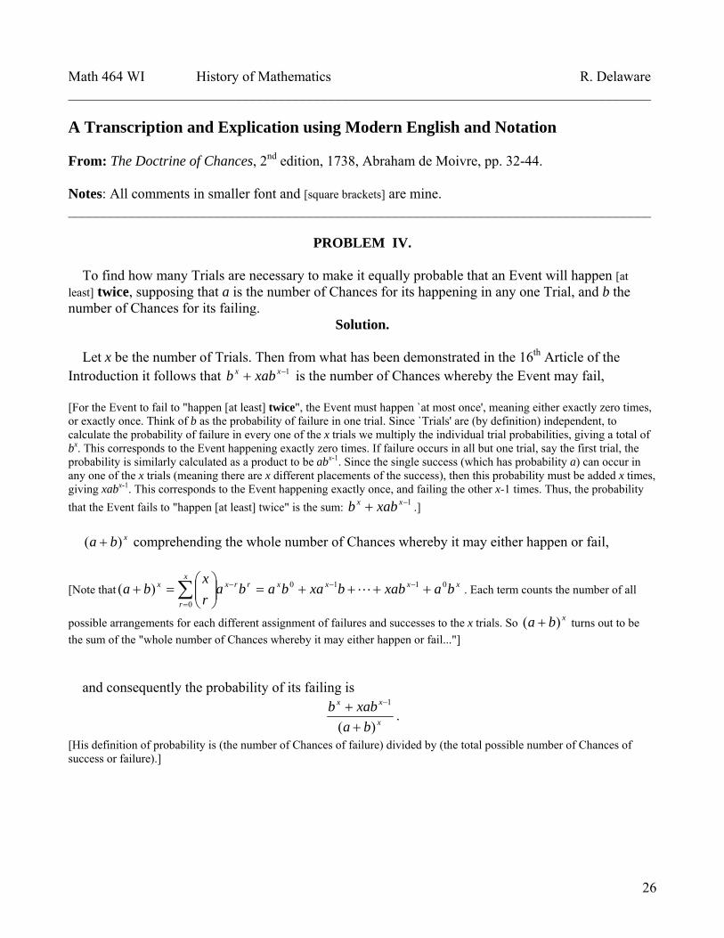
Math 464 WI History of Mathematics R. Delaware __________________________________________________________________________________ A Transcription and Explication using Modern English and Notation From: The Doctrine of Chances, 2nd edition, 1738, Abraham de Moivre, pp. 32-44. Notes: All comments in smaller font and [square brackets] are mine. __________________________________________________________________________________

PROBLEM IV. To find how many Trials are necessary to make it equally probable that an Event will happen [at least] twice, supposing that a is the number of Chances for its happening in any one Trial, and b the number of Chances for its failing.

Solution. Let x be the number of Trials. Then from what has been demonstrated in the 16th Article of the Introduction it follows that 1−+ xx xabb is the number of Chances whereby the Event may fail, [For the Event to fail to "happen [at least] twice", the Event must happen `at most once', meaning either exactly zero times, or exactly once. Think of b as the probability of failure in one trial. Since `Trials' are (by definition) independent, to calculate the probability of failure in every one of the x trials we multiply the individual trial probabilities, giving a total of bx. This corresponds to the Event happening exactly zero times. If failure occurs in all but one trial, say the first trial, the probability is similarly calculated as a product to be abx-1. Since the single success (which has probability a) can occur in any one of the x trials (meaning there are x different placements of the success), then this probability must be added x times, giving xabx-1. This corresponds to the Event happening exactly once, and failing the other x-1 times. Thus, the probability that the Event fails to "happen [at least] twice" is the sum: 1−+ xx xabb .] xba )( + comprehending the whole number of Chances whereby it may either happen or fail,

[Note that ∑=

−−− ++++=⎟⎟⎠

⎞⎜⎜⎝

⎛=+

x

r

xxxxrrxx baxabbxababarx

ba0

0110)( L . Each term counts the number of all

possible arrangements for each different assignment of failures and successes to the x trials. So xba )( + turns out to be the sum of the "whole number of Chances whereby it may either happen or fail..."] and consequently the probability of its failing is

x

xx

baxabb

)(

1

++ −

.

[His definition of probability is (the number of Chances of failure) divided by (the total possible number of Chances of success or failure).]

27

But, by Hypothesis, the Probabilities of happening and failing are equal. [Meaning, both must equal 1/2 (that is, they are "equally probable".)] We have therefore the Equation

21

)(

1

=+

+ −

x

xx

baxabb , or

122)( −+=+ xxx xabbba , or

making qb

a 1= ,

qx

q

x2211 +=⎟⎟

⎠

⎞⎜⎜⎝

⎛+ .

[That is, divide the equation 122)( −+=+ xxx xabbba by bx and then substitute qb

a 1= .]

Now if in this Equation we suppose q = 1, x will be found = 3, [Substituting q = 1 we get xx 222 += , hence xx +=− 12 1 . A little guessing shows that x = 3 (trials) satisfies the equation. (There is no algebraic way to solve this equation, and a simultaneous graph of the functions on either side of the equality only reveals that there is a single intersection point at

which x is positive.) Note that since both a > 0 and b > 0, then it follows from qb

a 1= that q > 0. Then q = 1 is the smallest

possible integral value of q here (its lower bound value).]

and if we suppose q infinite, and also zqx= , we shall have the Equation

)1log()2log( zz ++= ,

[To make sense of these statements, first observe that we can rewrite the equation above, with zqx= , as

qx

q

x2211 +=⎟⎟

⎠

⎞⎜⎜⎝

⎛+

⎟⎟⎠

⎞⎜⎜⎝

⎛+=

⎟⎟

⎠

⎞

⎜⎜

⎝

⎛⎟⎟⎠

⎞⎜⎜⎝

⎛+

qx

q

qx

q

1211

( )zq

zq

+=⎟⎟

⎠

⎞

⎜⎜

⎝

⎛⎟⎟⎠

⎞⎜⎜⎝

⎛+ 1211 .

Second, we recall the well-known calculus fact that as q→∞ we have

eq

q

→⎟⎟⎠

⎞⎜⎜⎝

⎛+

11

where e ≈ 2.71828 is the usual base for the natural exponential function, what he elsewhere calls the `hyperbolic base'. Thus, "if we suppose q infinite" we have )1(2 ze z += and then applying the logarithm function (to the `hyperbolic base') to both sides we find

28

)]1(2log[)log( ze z += )1log()2log( zz ++= .]

in which taking the value of z, either by Trial or otherwise, it will be found = 1.678 nearly. [Again, there is no algebraic way to solve this equation, or the equivalent equation )1(2 ze z += . A simultaneous graph of the functions on either side of the equality once again only reveals that there is a single intersection point at which z is positive. But from this, or numerical trial and error, we can approximate the solution as z ≈ 1.678.] And therefore the value of x will always be between the limits 3q and 1.678q, but will soon converge to the last of these limits. For which reason, if q be not very small, x may in all cases be supposed = 1.678q.

[The equation zqx= can be written as x = zq. So from above, when q = 1 we found that x = 3, which here we write as x =

3q. From the last calculation, for large values of q (that is, as q→∞) we found that x ≈ 1.678q, meaning x "will soon converge to" this value.] Yet if there be any suspicion that the value of x thus taken is too little, substitute this value in the original Equation

qx

q

x2211 +=⎟⎟

⎠

⎞⎜⎜⎝

⎛+ ,

and note the Error. Then if it be worth taking notice of, increase a little the value of x, and substitute again this new value of x in the aforesaid Equation. And noting the new Error, the value of x may be sufficiently corrected by applying the Rule which the Arithmeticians call double false Position.

[For instance, note first that the absolute error function x

qqx

⎟⎟⎠

⎞⎜⎜⎝

⎛+−+

1122 is an increasing function of x, the number of

trials. Now, suppose that error function equals e1, “the Error”. Next, “increase a little the value of x”, by say 0>δ . Then

we have 211)(22 eqq

xx

=⎟⎟⎠

⎞⎜⎜⎝

⎛+−

++

+δδ

, “the new Error”. We now have two points, ),(),,( 21 exex δ+ , where

21 ee < . Where a line through these two points intersects the x-axis is our “double false Position” (linear) approximation of the true value of x = the number of trials.] __________________________________________________________________________________

29

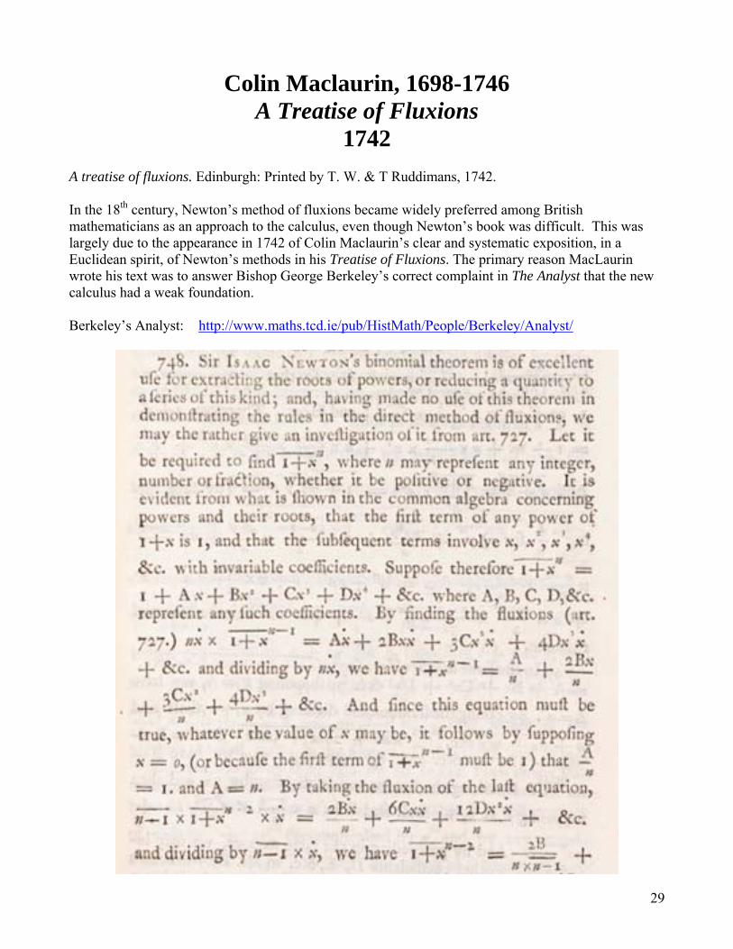
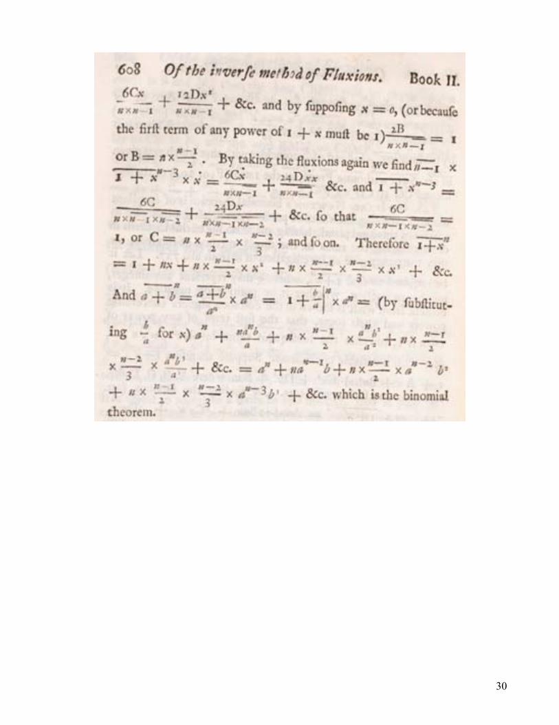
Colin Maclaurin, 1698-1746 A Treatise of Fluxions

1742 A treatise of fluxions. Edinburgh: Printed by T. W. & T Ruddimans, 1742. In the 18th century, Newton’s method of fluxions became widely preferred among British mathematicians as an approach to the calculus, even though Newton’s book was difficult. This was largely due to the appearance in 1742 of Colin Maclaurin’s clear and systematic exposition, in a Euclidean spirit, of Newton’s methods in his Treatise of Fluxions. The primary reason MacLaurin wrote his text was to answer Bishop George Berkeley’s correct complaint in The Analyst that the new calculus had a weak foundation. Berkeley’s Analyst: http://www.maths.tcd.ie/pub/HistMath/People/Berkeley/Analyst/

30

31

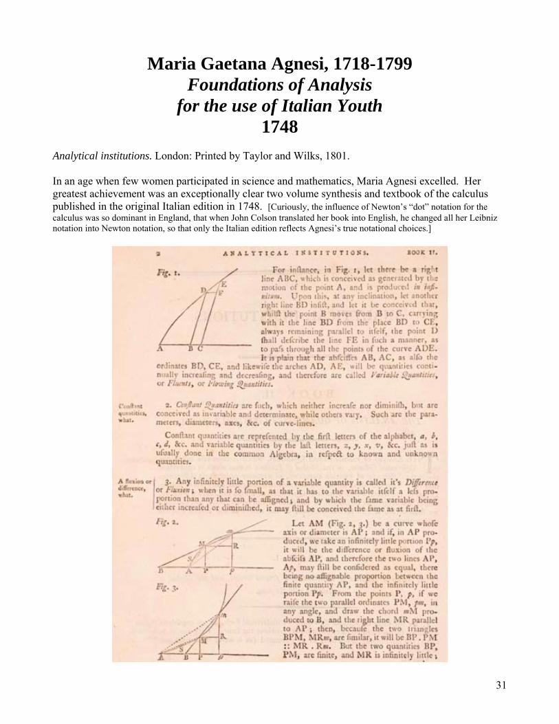
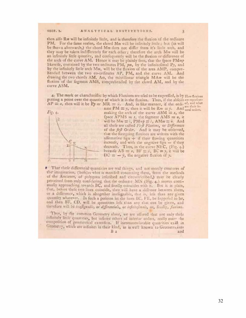
Maria Gaetana Agnesi, 1718-1799 Foundations of Analysis

for the use of Italian Youth 1748

Analytical institutions. London: Printed by Taylor and Wilks, 1801. In an age when few women participated in science and mathematics, Maria Agnesi excelled. Her greatest achievement was an exceptionally clear two volume synthesis and textbook of the calculus published in the original Italian edition in 1748. [Curiously, the influence of Newton’s “dot” notation for the calculus was so dominant in England, that when John Colson translated her book into English, he changed all her Leibniz notation into Newton notation, so that only the Italian edition reflects Agnesi’s true notational choices.]

32

33

How I use these books, and their translations, for my History of Mathematics class at UMKC

If the use of the history of mathematics in the classroom is to be more than a collection of generic and occasionally entertaining stories, as instructors we need to dig deeper. We need to look at the actual historical written work of mathematicians and teachers of mathematics to see how they were thinking in the context of their times. Luckily we now have access to many excellent English translations of historical mathematics, and though as working teachers we don’t have time to do a comprehensive archaeological excavation into them, we can dig “test-pits” to dip into that rich past. The struggles of the historical mathematics research community toward understanding, when it first encountered the very same issues that our students now perennially face in learning elementary mathematics, can engage those students, if we take advantage of the universal human pleasure in detective work. I present my students with copies of historical arguments, problem solutions, or proofs (with some guiding notes), and often tell them little (until after the assignment) about the author, or his or her time period. So, they are faced with extracting meaning from material that is well within their grasp, but unusual in presentation. With the power of modern notation at their fingertips, along with the hundreds and sometimes thousands of years of mathematical sophistication since the material was written, they successfully learn to read with precision and to explicate the given arguments and proofs, and in the process build confidence in their own work. They even find this exciting, especially when I reveal who the author is. __________________________________________________________________________________

Explicate, verb, [Definition, Oxford English Dictionary]: 1.a. To unfold, unroll; to smooth out (wrinkles); to open out (what is wrapped up): to expand…

c. To spread out to view, display. 2. a. To disentangle, unravel.

3. To develop, bring out what is implicitly contained in (a notion, principle, proposition.) 4. To unfold in words; to give a detailed account of …

6. To make clear the meaning of (anything); to remove difficulties or obscurities from; to clear up, explain. __________________________________________________________________________________

34

Historical “Proof” Explication

• Read the given argument, proof, or theorem and proof combination. I have photocopied them from an original historical document, or faithful English translation. The assignment is designed to be more-or-less self-contained.

• Explicate this result, that is, to write an expository version. Your version will usually therefore be

longer than the original. Remember that a “proof” is a narrative, telling the story of (proving) why the theorem is true. Your job is to make that story transparent.

• Stay as close as possible to the style and form of the argument, preserving the historical flavor

and ideas of the author. Do not substitute a faster, modern statement and proof. • You will be graded on the clarity of your exposition. • You will also be graded on how critically you have read the result, whether you found all the

confusions, omitted arguments, and so on, even if you were not able to settle all of them to your satisfaction.

• Your work may require any or all of the following:

• Clarify words, definitions, and statements. For instance, "line" may be used where "line segment" is meant, "equation" confused with "expression", or "equal" with "congruent" or "equivalent"; the same letters or words may be used for several different objects; out-of-date terminology and phrasing may need to be updated, or just made more precise.

• Is the result properly stated as a Theorem, Proposition, Lemma, Corollary, etc.? Is the Proof

so named, and clearly delineated? • Add as many pictures as you like to clarify the argument. These include "idea" pictures, as

well as the usual graphs, diagrams, constructions, etc. A detailed “movie” of images is often needed.

• Include omitted arguments, or other details. Some arguments may be long enough to be

stated (by you) separately as a Lemma. Do so, if you like. Other arguments may be assumed common knowledge by the author, but not clear to you or your modern readers. Tell us. This is vital to good exposition.

• Correct any mathematical errors or omissions you may find. For example, if a variable

suddenly appears in a denominator, did the author consider the case when that variable might be zero? Are there other omissions of cases we would today include? Are there typographic errors? Are the calculations really correct? Take nothing for granted.

• Modernize the mathematical notation if needed, but again, stay close to the history.

_________________________________________________________________________________