Embed Size (px)
Citation preview

NCHRP Project 14-20A Final Report
G - 1
A P P E N D I X G
Procedure to Quantify Consequences of Delayed Maintenance of Lighting
The purpose of roadway lighting is to provide better nighttime visibility conditions for drivers to improve
safety and reduce the risk of nighttime crashes (Lutkevich et al. 2012). “Lighting enables the driver to recognize
the geometry and condition of the roadway at extended distances” (ILDOT 2013). Street lighting improves
visibility and safety of pedestrians on sidewalks, reduces crime, as well as well-lit crosswalks improve visibility
of pedestrians for incoming vehicles. Lighting also increases road aesthetics and helps to maintain operating
speed during nighttime (Markow 2007). Delaying maintenance on the lighting system will not only impact
agency future maintenance and replacement costs but will also affect safety increasing the likelihood of car
crashes at nighttime. Figure G-1 shows the procedure to quantify the consequences of delayed maintenance of
lighting systems.
Figure G-1. Procedure to quantify the consequences of delayed maintenance of lighting.
Figure G-1. Procedure to quantify the consequences of delayed maintenance of lighting.
Scenario 1
All Needs
Future budget needs:
- Maintance and Replacement Cost
- Backlog Cost
- Crash Cost
- Energy Cost
Lighting System Condition
Lighting System Value and Sustainability
Ratio
Step 3: Conduct Delayed
Maintenance Scenarios
Analyses
Step 2: Determine
Maintenance and Budget
Needs for the Lighting
System
Step 1: Define the Lighting
System Preservation Policy
Scenario 2
Do Nothing
Scenario 3
Delayed Maintenance
1.1: Identify the Types of Maintenance
1.2: Establish Performance Objectives for the Lighting System
1.3: Formulate Decision Criteria for Lighting Maintenance Activities
2.1: Assess the Lighting System Condition and Service Life
3.1: Formulate Delayed Maintenance Scenarios
3.2: Perform the Delayed Maintenance Scenarios Analyses
3.3: Determine the Impact and Report the Consequences of
Delayed Maintenance
2.2: Select Performance Models to Forecast the Lighting Condition
2.3: Perform the Needs Analysis
Scenario 4
Budget-Driven with
Limited Funds
Percentage of Lighting in Service

NCHRP Project 14-20A Final Report
G - 2
G.1 Step 1: Define the Lighting System Preservation Policy
The initial step in the procedure is to define a preservation policy for the lighting system. To some extent the
level at which the policy is defined depends on the data that an organization has available on its lighting assets.
For instance, if an organization has detailed data on the inventory, with details on structural supports and their
condition, electrical systems, and dates of the most recent relamping of each system, then it is possible to define
a relatively comprehensive and specific policy. However, many organizations maintain a basic database of
lighting assets with very high-level inventory and little or no condition data. In these cases, the preservation
policy is necessarily more straightforward, identifying under what circumstances relamping is performed. The
following sections describe the sub-steps in defining a system preservation policy regardless of the level of
detail of the inventory and condition data that an organization maintains. The example presented in this
Appendix illustrates a case for an agency that has only summary inventory data on its database as available in
most of the DOTs.
G.1.1 Identify the Types of Maintenance
In this step the agency must determine what types of maintenance should be considered in the preservation
program. This is complex by the fact that the term “maintenance” is often defined differently between agencies.
Common maintenance terms for lighting used by DOTs are defined as follows:
Preventive maintenance is usually targeted on switch gear, control cabinets, (Markow 2007) or cleaning. The
frequency of luminaire cleaning is calculated based on the Luminaire Dirt Depreciation (LDD) factor which
accounts for characteristics such as “luminaire type, mounting height, environment of the luminaire location
(urban or rural setting), traffic volume, and roadway offsets” (AASHTO 2005).
Immediate maintenance, also called remedial, is often performed in emergency safety hazard cases, such as
knockdowns, cable breaks, and switch gear problems (Markow 2007).
Corrective maintenance is usually performed on fixture failures and any problems with the lamp or ballast
(Markow 2007).
Worst-first maintenance is performed on “underground breaks from deteriorated systems resulting in failures
from salt water and freeze-thaw in winter” (Markow 2007).
Group replacement / Routine maintenance: Lighting systems can be replaced at a specified interval. In the
European Union, where lighting is of high quality with very few outages, the lighting systems are relamped
typically every three or five years (Wilken et al. 2001). Older facilities may need to be updated to the current
light sources, energy conservation standards and wiring (ILDOT 2013 and MnDOT 2010). There is an incentive
to replace high-pressure sodium (HPS) luminaires with light-emidding diodes (LEDs) which are more energy
efficient and last longer.
Some DOTs perform mostly corrective maintenance due to low manpower and non-existing processes for
selecting which lighting asset components are maintained. Accidents and electrical faults get priority and
monthly night runs are performed to find problems. Work orders are processed via various management
systems, for example SAP, where history of maintenance costs are saved. Often there are not statewide policies
and management plans for lighting, so the maintenance practices differ from region to region. However, it is
recommended by FHWA to include a maintenance plan (cleaning and replacement) in the life-cycle cost
analysis during design stages, as in some cases, more expensive durable and corrosion-resistant lighting can
provide the best benefit to cost ratio (Lutkevich et al. 2012).
In the lighting model developed in this study, the number and type of maintenance activities for the
preservation of the lighting system has been streamlined to include proactive relamping (replacing lamps prior
to failure), reactive relamping (replacing lamps after they have failed), and installation of new LED lights to
replace HPS lights.
NCHRP Project 14-20A Final Report
G - 3
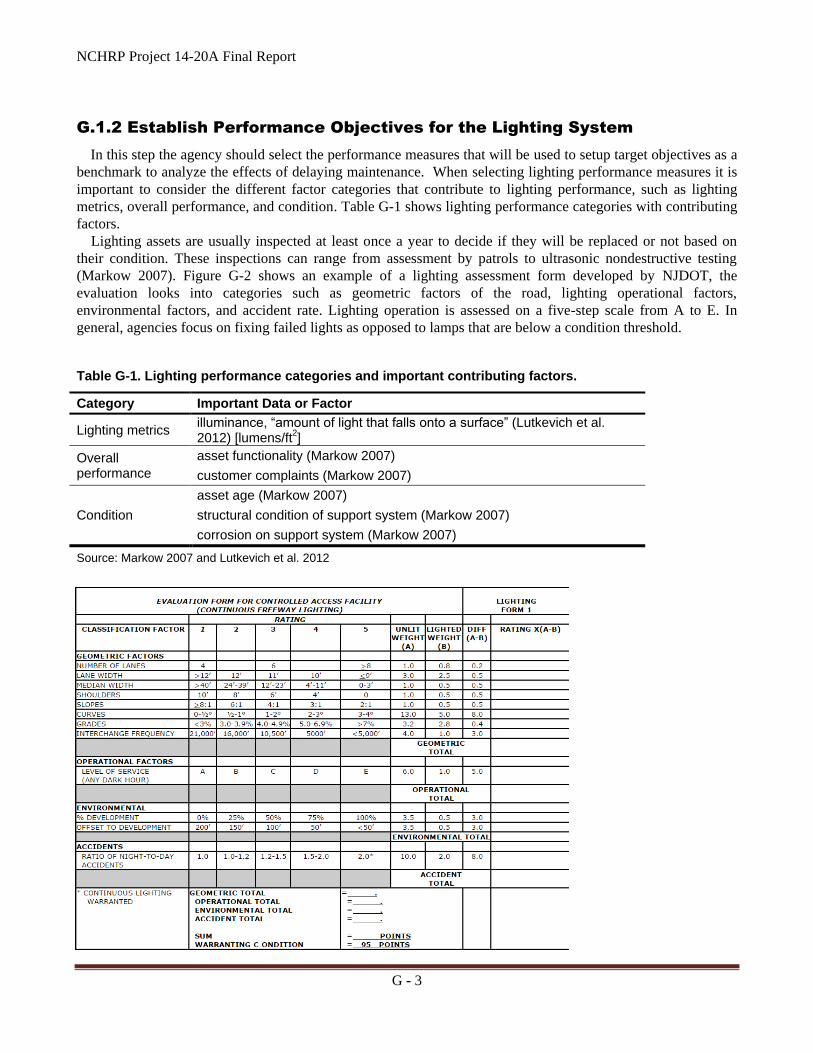
G.1.2 Establish Performance Objectives for the Lighting System
In this step the agency should select the performance measures that will be used to setup target objectives as a
benchmark to analyze the effects of delaying maintenance. When selecting lighting performance measures it is
important to consider the different factor categories that contribute to lighting performance, such as lighting
metrics, overall performance, and condition. Table G-1 shows lighting performance categories with contributing
factors.
Lighting assets are usually inspected at least once a year to decide if they will be replaced or not based on
their condition. These inspections can range from assessment by patrols to ultrasonic nondestructive testing
(Markow 2007). Figure G-2 shows an example of a lighting assessment form developed by NJDOT, the
evaluation looks into categories such as geometric factors of the road, lighting operational factors,
environmental factors, and accident rate. Lighting operation is assessed on a five-step scale from A to E. In
general, agencies focus on fixing failed lights as opposed to lamps that are below a condition threshold.
Table G-1. Lighting performance categories and important contributing factors.
Category Important Data or Factor
Lighting metrics illuminance, “amount of light that falls onto a surface” (Lutkevich et al. 2012) [lumens/ft
2]
Overall performance
asset functionality (Markow 2007)
customer complaints (Markow 2007)
Condition
asset age (Markow 2007)
structural condition of support system (Markow 2007)
corrosion on support system (Markow 2007)
Source: Markow 2007 and Lutkevich et al. 2012

NCHRP Project 14-20A Final Report
G - 4
Source: NJDOT 2014
Figure G-2. Example of a lighting assessment form.
Lighting standards, warrants, and design criteria are found in the Roadway Lighting Design Guide (AASHTO
2005), and the ANSI / IES RP-8-14: American National Standard Practice for Roadway Lighting. For example,
the ANS/IES standard defines the recommended luminance based on roadway classification (major, collector,
local) and pedestrian traffic at night (significant, lesser, low traffic) (MnDOT 2010). The lighting equipment
consists of luminaires, support system, and service cabinets. Luminaires have optical, electrical, and mechanical
components Lighting support system consists of mast arm, pole, and foundation.
The targets clearly depend largely upon what performance measures are established. The following are
examples of targets an agency might set for common performance measures:
Percentage of lighting in certain condition
Lighting age
Degree of lighting material degradation
Other lighting performance measures used by DOTs are shown in Table G-2.
Table G-2. Examples of other performance measures for lighting.
Performance Measure Description Source
Function as intended 90% of the total luminaries of the combined sign and
highway lighting are functioning as intended FDOT 2015
Crash rate Ratio of night-to-day accidents NJDOT 2014
Energy savings Percentage of LEDs, Percentage converted to LEDs
In this study, the lighting model predicts the percentage of lights in operation at a given point. When
lights fail, this reduces energy costs but increases accident costs. The model predicts that the nighttime crash
rate increases 33 percent at a given location when lighting is not functioning (equivalent to a 25 percent decrease
for adding lighting to an unlit location). This crash rate estimate is based on a recent synthesis on effects of
lighting on safety (Wilken et al. 2001). To use the model, targets are specified for proactive relamping, reactive
replacement of failed lamps, and conversion to LED. The model predicts the needs for reactive replacement of
failed lamps, and funds necessary to achieve the target values during the analysis period.
G.1.3 Formulate Decision Criteria for Maintenance Activities
The decision criteria should specify what activities are needed based on the lighting condition and the cost of
those activities. Later in the process, it is necessary to further determine the impact of the activities on lighting
condition. If an agency has implemented a lighting management system, then this information may already be
specified; otherwise it is necessary to define the maintenance activities. In order to simplify the decision criteria,
maintenance activities are divided into two major groups:
Proactive maintenance: Agencies not only fix failed lamps, but also lamps that have a greater probability of
failure if they are below a certain threshold. For example, a DOT can plan for rewiring of old direct bury wires
to reduce future failures and proactively retrofit lighting fixtures to LED.
Reactive maintenance: Agencies fix lamps only when they have failed. For example, Colorado Department
of Transportation Region 5, assess condition of a certain percentage of their lighting asset inventory and replace
any lights that are not in good condition. Other agencies, such as Texas Department of Transportation, monitor
condition remotely via voltage, where a drop in voltage indicate a knockdown or a burnt out lamp.

NCHRP Project 14-20A Final Report
G - 5
In this study, the lighting model simulates reactive maintenance by allowing the user to specify what percent
of failed lamps are replaced each year (ideally 100 percent but possibly less in practice if maintenance is
delayed). Further, the model simulates proactive replacements by allowing the user to specify the probability
threshold at which lamps are proactively replaced. For example, if the user enters a value of 90 percent, then
any lamps that have a 90 percent chance of failure (or greater) in a given year are replaced. Also, the user can
specify what percentage of conventional HPS fixtures are converted to LED each year.
G.2 Step 2: Determine Maintenance and Budget Needs for the Lighting
System
G.2.1 Assess the Lighting System Condition
Lighting service life is usually determined based on agency experience, professional judgment and
manufacturer’s data. However, assets are often “repaired or replaced as soon as they fail without regard to
service life” (Markow 2007). Group relamping based on lamp mortality curve based on manufacturer’s data is a
common maintenance method (CDOT 2006). DOTs perform nighttime drive-by inspections looking for
problems such as flickering or knockdowns, usually in less than three month intervals (Markow 2007). Highway
lighting is monitored more often, e.g. every two weeks.
The median life expectancy for lighting ranges between 25 to 30 years for structural components, 1 to 4 years
for lamps, 7 years for ballast, 18 years for control panels and 16 years for luminaires, as Table G-3 shows. LED
lamps are not shown on the table. These are projected to last 10 to 20 years (similar to that shown for a typical
luminaire), but when they fail the LED fixture must be replaced rather than an individual lamp.
Table G-3. Lighting life expectancy.
Components and Material
No. of Responses
Minimum (Years)
Maximum (Years)
Mean (Years)
Median (Years)
Mode (Years)
Structural Components
Tubular Steel 12 10 40 25.4 25 25
Tubular Aluminum 9 10 40 26.1 25 30
Cast Metal 2 15 30 22.5 22.5 −
Wood Posts 2 25 40 32.5 32.5 −
High mast or tower 11 10 50 28.6 30 30
Lamps
Incandescent 3 1 5 2 1 1
Mercury Vapor 6 3 5 4 4 4
High pressure 15 1 6 3.6 4 5
Sodium
Low-pressure 3 1 5 3 4 4
Sodium
Metal halide 9 1 5 2.9 3 2
Fluorescent 1 − − 5 − −
Other components
Ballast 9 2 25 9.7 7.5 10
Photocells 11 1 10 5.2 5 5
Control panels 7 10 25 18.2 20 20
Luminaires 2 5 25 16.25 16.25 −
Notes: −, value is undefined for the particular distribution. When distribution is based on only one data point, its value is

NCHRP Project 14-20A Final Report
G - 6
shown in the Mean column.
Source: NCHRP Synthesis 371 – Markow 2007
G.2.2 Select Performance Models to Forecast the Lighting System Service
Life
Lighting performance can be estimated based on condition or age. A condition-based approach requires
periodical condition assessment inspections to develop deterioration models. An age-based approach estimates
the remaining life from historical records of construction and reconstruction. For lighting systems an age-based
approach is frequently the only viable approach as it is often not practical to establish a condition assessment
program for lighting, and it is difficult to visually inspect conditions of key components, such as lamps. Popular
performance models used to forecast lighting service life include:
Exponential functional form (Szary et al. 2005)
Weibull distribution (Ford et al. 2012)
Table G-4 shows an example of a Weibull regression model to predict roadway lighting life.
Table G-4. Weibull regression model of roadway lighting life (end-of-life = historical replacement
interval).
Source: Ford et al. 2012
The lighting failure probability can follow a Weibull distribution as Figure G-3 shows. Failure probability
increases for metal and tall poles. Whereas factors such as “warmer climate, sign mounting and interstate”
location tend to extend the life (Ford et al. 2012). A Kaplan-Meier (K-M) estimate distribution is also shown in
Figure G-3. The prediction of Weibull model was validated against the non-parametric K-M estimate (Ford et al.
2012).
Life Expectancy Factor Parameter Estimate, β
t-Statistic
Constant -4.674 -1.479
Normal Annual Temperature (°F) 0.172 2.933
Material type indicator (1 if metal pole, 0 otherwise) -1.023 -7.964
Mounting location indicator (1 if on sign, 0 otherwise) 1.069 3.113
Functional class indicator (1 if on interstate, 0 otherwise) 0.437 3.440
Fixture height indicator (1 if less than 30 feet, 0 otherwise) -0.350 -1.391
Baseline Ancillary Factors Parameter
Estimate, β t-Statistics
Shape Factor, β 1.764 14.201
Scaling Factor, α 123.609 10.372
Model Statistics
Number of observations 229
Log-likelihood Function at Convergence -177.88
Restricted Log-likelihood Function -328.68

NCHRP Project 14-20A Final Report
G - 7
Source: Ford et al. 2012
Figure G-3. Lighting failure probability curve.
In this study, the lighting model uses a Weibull distribution that predicts lamp failure. Default values for the
model were populated based on findings from the NCHRP Report 713 and expert knowledge. This modeling
approach is consistent with existing practices, but focuses on failure of the shortest-lived element of a lighting
unit, the lamp, and does not account for the need for maintenance of structural or electrical components. Figure
G-4 illustrates the cumulative failure probability assumed in the model for HPS lamps and LED fixtures. As
indicated in the figures, HPS lamps are predicted to last 2-3 years, and LED fixtures are predicted to last
approximately 20 years based on this model.
Figure G-4. Modeled failure rate of HPS lamps and LED fixtures.

NCHRP Project 14-20A Final Report
G - 8
G.2.3 Perform the Needs Analysis
The needs analysis is performed as follows using the lighting model developed for the research:
1. HPS lamps and LED fixtures are grouped by age in years, and calculations are made for each 1-year age
bin (e.g., 2-year old HPS lamps).
2. Three types of needs are considered: (1) needs for replacing failed HPS lamps and LED fixtures; (2)
needs for proactively replacing HPS lamps or LED fixtures with a specified probability of failure, and
(3) needs for conversion from HPS to LED lamps.
3. The model predicts the number of failed lamps and fixtures for each 1-year age bin using the
distributions shown in Figure G-4. The percentage of failed lamps/fixtures replaced is specified as
input, as is the average amount of time between the initial failure and lamp/fixture replacements.
4. For each age bin the model predicts the likelihood of failure in the next year for the HPS lamps and
LED fixtures that do not fail in the current year. If the failure likelihood exceeds a specified percentage,
then these lamps/fixtures are replaced.
5. The model predicts the number of HPS lights converted to LED. The percentage converted is an input
specified by analysis year and the same value is applied regardless of age.
6. Agency costs are tabulated for reactive replacements, proactive replacements, and conversion to LED.
7. Energy costs are tabulated, accounting for the savings in energy cost from not operating failed lights,
and the reduced energy costs of LED relative to HPS.
8. Crash costs due to failed lights are tabulated, accounting for the number of failed lights and failure
duration. The model predicts increased crash costs from nighttime crashed based on the model
assumptions detailed further below.
9. Lamp/fixture ages are increased by one year, and the analysis is repeated for the next year until the end
of the analysis period.
Table G-5 lists the default lighting model assumptions with the corresponding notes of the source. Regarding
replacement costs, the cost for HPS is based on data from Virginia described in the literature (VTRC 2015).
This study estimates annual maintenance costs, including costs of relamping and other maintenance, and
expresses them as a unit cost per watt per year. These are captured in the average replacement cost of $480 for
HPS based on the assumption that HPS fixtures are typically 250W and are relamped every two years. This
reference estimates similar costs for LED on a per year basis. However, the unit cost per replacement is
significantly higher, $3,000 per replacement, since LED fixtures are replaced less frequently. If replacement
work is performed reactively rather than proactively (unscheduled rather than scheduled), it is assumed to add
10 percent to the cost. Other parameters, including energy costs, time to replace failed lamps/fixtures, crash-
related parameters, and the existing inventory are based on data collected in the case study.

NCHRP Project 14-20A Final Report
G - 9
Table G-5. Default lighting model assumptions.
G.3 Step 3: Conduct Delayed Maintenance Scenarios Analyses
G.3.1 Formulate the Delayed Maintenance Scenarios
Table G-6 defines the set of scenarios evaluated for lighting maintenance. In Scenario 1, three different types
of agency-desired maintenance policies are tested. Scenario 1.a approximates the current practices of an agency
in located in western state. In this case, lighting maintenance is performed in a reactive manner: when an HPS
lamp or LED fixture fails, it is replaced, and the agency is gradually transitioning from use of HPS to LED.
However, the agency does not perform proactive replacements of HPS or LED. Scenario 1.b describes a
scenario in which failed HPS lamps and LED are replaced, and the agency is also proactively gradually
transitioning from use of HPS to LED over a 10 year period. In addition, the agency proactively replaces units
with high probability of failure, reducing replacement costs and the time that lights are out. Scenario 1.c is
similar to Scenario 1.a, except that in this case no additional fixtures are transitioned from HPS to LED.
In Scenario 2, replacement of failed lamps is delayed by 10 years. In Scenario 3, the replacement of failed
lamps/fixtures is delayed by 5 years. In Scenario 4 different constraints are placed on maintenance work. In
Scenario 4 only a percentage of failed lamps are replaced due to limited budget. Percentages are include 90
percent in Scenario 4.a, 75 percent in Scenario 4.b, and 50 percent in Scenario 4.c.
Parameter Value Notes
Annual energy cost per fixture ($)
HPS 78.40 Energy cost of 7 cents per kWh assumed based on case study assuming 4,000 hours of energy use per fixture, with 250W per fixture for HPS, 150W for LED
LED 47.04
Replacement cost per unit ($)
HPS, scheduled 480 (VTRC 2015): determined based on analysis of annual maintenance costs for HPS lighting: 10% increase assumed for unscheduled replacement Case study data: 10% increase assumed for unscheduled replacement
HPS, unscheduled 528
LED, scheduled 3,000
LED, unscheduled 3,300
Time to replace failed lamp/fixture (days) 14 Case study data
Annual VMT for portion on network with lighting (millions)
1,484.64 Case study data: 12% of network of interstates, other freeway/expressway and other principal arterials.
Nighttime crash rate for portion of network with lighting (crashes per million VMT)
1.65 Case study data: note the analysis assumes half of all crashes occur at night
Average crash cost ($/crash) 100,000
Case study data
Initial number of fixtures HPS 4,510
LED 5,723

NCHRP Project 14-20A Final Report
G - 10
Table G-6. Key elements to analyze delayed maintenance scenarios for lighting.
Data Performance
Models Maintenance Scenarios
Length of Analysis: 10 years Results
Lighting System Database Inventory
Weibull models for predicting likelihood of lamp or electrical failure Another alternative to model deterioration is a straight-line service life, based on original design life
1. All Needs
a. Failed lamps/fixtures are replaced in 2 weeks. HPS
is replaced with LED over a 10-year period. No additional proactive replacements are performed.
b. Failed lamps/fixtures are replaced in 2 weeks. HPS is replaced with LED over a 10-year period. Additionally, lamps/fixtures are proactively replaced when their failure probability exceeds 90%.
c. Failed lamps/fixtures are replaced in 2 weeks. No proactive replacements are performed and no additional fixtures are converted to LED.
2. Do Nothing
All lamp/fixture replacements are deferred for 10 years.
3. Delayed Maintenance All lamp/fixture replacements are deferred for 5 years. After the deferral period failed lamps are replaced in two weeks. No proactive replacements are performed and no additional fixtures are converted to LED.
4. Budget-Driven with Limited Funds
a. Only 90 percent of failed lamps/fixtures are replaced due to limited budget
b. Only 75 percent of failed lamps/fixtures are replaced due to limited budget
c. Only 50% of failed lamps/fixtures are replaced due to limited budget
Replacements that are performed in 2 weeks. No proactive replacements are performed, and no additional fixtures are converted to LED.
Analytical Tool Spreadsheet based model that incorporates probability of failure Reports
Impact on condition due to delayed maintenance
Agency costs of scheduled and unscheduled maintenance
Agency costs of converting HPS to LED where applicable
Agency energy costs
Increased user accident costs from loss of lighting

NCHRP Project 14-20A Final Report
G - 11
G.3.2 Perform the Delayed Maintenance Scenarios Analyses
Table G-7 shows the results of the scenarios described in Table G-6. Agency costs of replacing
lamps/fixtures reactively (unscheduled) and proactively (scheduled); the cost of converting from HPS to LED;
excess crash costs; energy costs; and total costs are reported. A discount rate of 7 percent is used for the
discounted costs. The minimum percentage of fixtures in service over the period of analysis and at the end of the
10 years are also reported.
Table G-7. Summary of scenario analysis results for lighting.
1 At the end of year 10
G.3.3 Determine the Impact of Delayed Maintenance and Report the
Consequences
To quantify the consequences of delayed maintenance, the results of delayed maintenance scenarios are
compared to the baseline scenario from the needs analysis. Six scenarios out of eight the scenarios defined in
Table G-7 are selected to show the consequences of delayed maintenance.
Consequences on the Lighting System in Service
Prior to the scenario analyses 100 percent of the lighting system is in service and 56 percent of the lights are
LED.
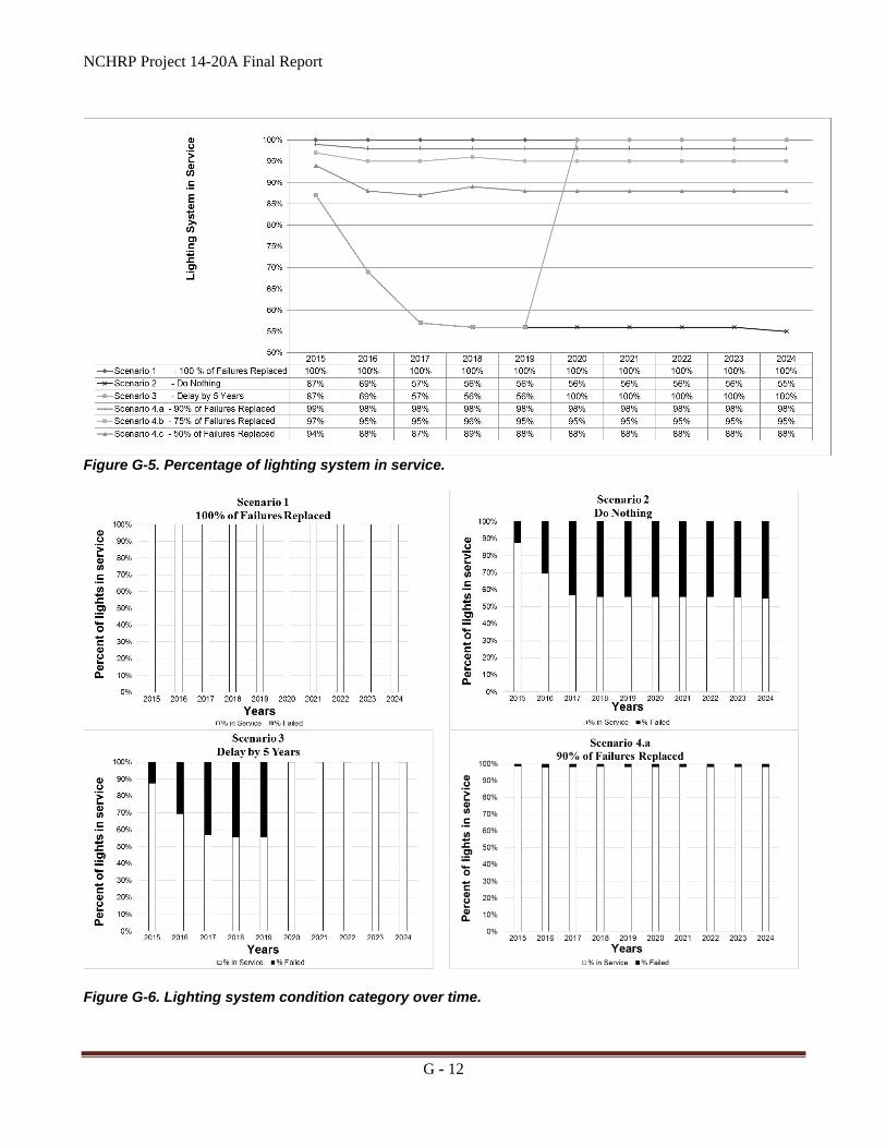
Figures G-5 and G-6 display the percentage of the lighting system in service throughout the analysis period.
For Scenario 1.a, where 100 percent of failures are replaced, the entire lighting system is in service during the
analysis period. This is representative of Scenario 1.b and 1.c, as well. For Scenario 2, where lamp
replacements are delayed by 10 years, the percentage of lighting system in service drops to 55 percent in year
10. For Scenario 3, where lamp replacements are delayed by 5 years, the percentage of lighting system in
service drops to 56 percent in year 5 and then recovers to 100 percent in year 6. For Scenario 4.a, where 90
percent of failures are replaced, 98 percent of the lighting system is in service during the analysis period. For
Scenario 4.b, where 75 percent of failures are replaced, 95 percent of the lighting system is in service during the
analysis period. For Scenario 4.c, where 50 percent of failures are replaced, 88 percent of the lighting system is
in service during the analysis period.
NCHRP Project 14-20A Final Report
G - 12
Figure G-5. Percentage of lighting system in service.
Figure G-6. Lighting system condition category over time.

NCHRP Project 14-20A Final Report
G - 13
Figure G-6. Lighting system condition category over time. (Continued)
Consequences on Future Budget Needs
Figure G-7 shows the predicted costs by year for Scenario 1.a, which best represents current agency practice.
The figure shows proactive and reactive replacement costs by year, costs for conversion from HPS to LED,
energy costs, crash costs, and total costs. Figure G-8 shows predicted costs by year for Scenario 1.c, in which
failed lamps and fixtures are replaced, but no additional fixtures are converted to LED. Relative to Scenario 1.a
there are no conversion costs, but these are substituted with higher energy costs and higher costs for reactive
replacements. Note that over the 10-year analysis period considered by the model Scenario 1.c is slightly
cheaper than Scenario 1.a. However, the benefits of LED over HPS are expected to manifest themselves over a
longer period than the 10-year analysis period, and in any case the purpose of the present analysis is to
demonstrate the effects of delaying maintenance, not the life-cycle implications of converting from HPS to
LED. Figure G-9 shows the predicted costs for Scenario 3, in which all work is deferred for 5 years. In this
scenario increased crash costs become the dominant cost over the deferral period, rising to approximately $20
million per year (equivalent to an additional 2-3 fatalities per year). Figure G-10 shows the predicted percentage
of lighting units in service for this scenario, illustrating the drop in HPS lighting in service over the deferral
period.
Figure G-7. Costs by year, Scenario 1.a.

NCHRP Project 14-20A Final Report
G - 14
Figure G-8. Costs by year, Scenario 1.c.
Figure G-9. Costs by year, Scenario 3.
Figure G-10. Lighting units in service by year, Scenario 3.

NCHRP Project 14-20A Final Report
G - 15
Figure G-11 shows the unfunded backlog for each scenario throughout the analysis period. For Scenario 1,
where 100 percent of failures are replaced, there is no backlog. For Scenario 2, where lamp replacements are
delayed by 10 years, the backlog is $2.7 million at year 10. For Scenario 3, where lamp replacements are
delayed by 5 years, the backlog reaches $2.4 million in year 5 but starting year 6 there is no backlog costs. For
Scenario 4.a, where 90 percent of failures are replaced, the backlog does not reach over $112,000 during the 10-
year analysis period. For Scenario 4.b, where 75 percent of failures are replaced, the backlog reaches $316,000
at the end of the analysis period. For Scenario 4.c, where 50 percent of failures are replaced, the backlog reaches
$768,000 at the end of the analysis period.
Figure G-11. Unfunded backlog for each scenario over the analysis period.
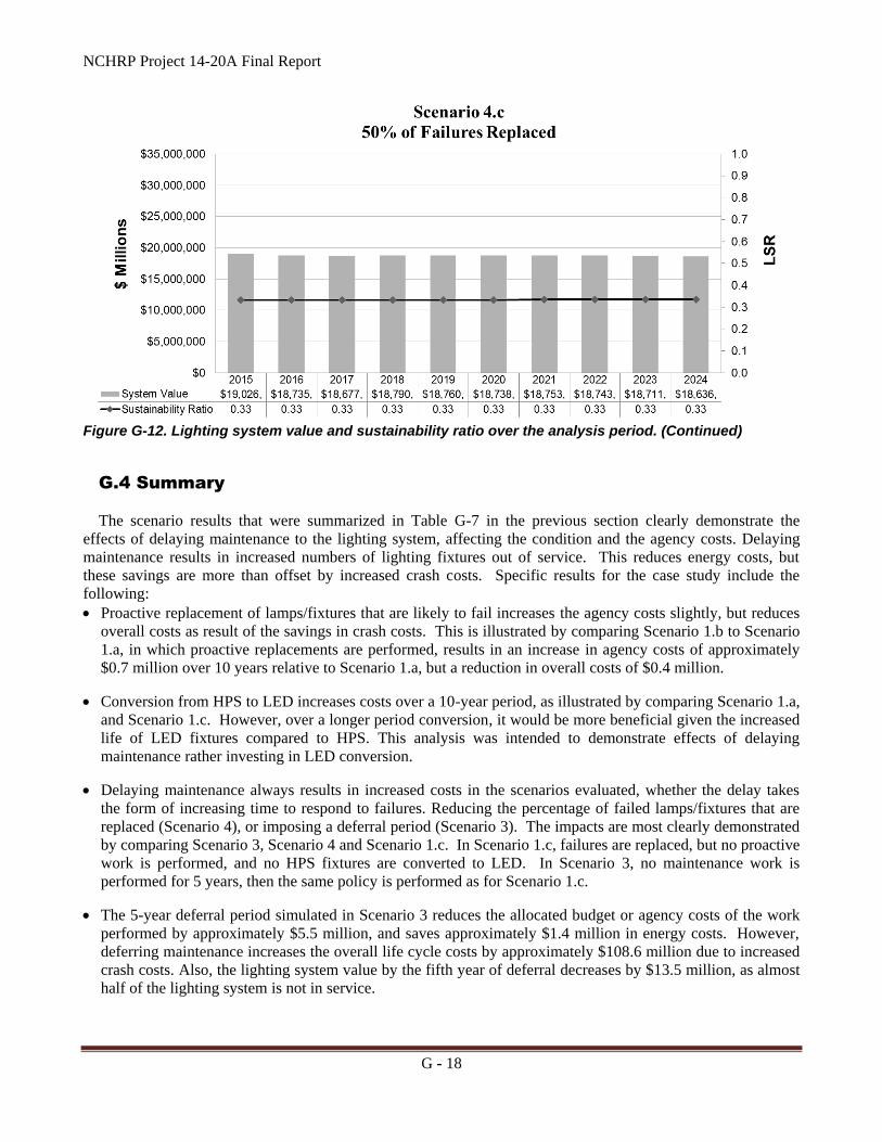
Figure G-12 shows changes of the lighting system value together with the lighting sustainability ratio (LSR)
over the analysis period of 10 years. LSR indicates on a scale 0 to 1 the percentage of asset needs that are
funded each year.

NCHRP Project 14-20A Final Report
G - 16
For Scenario 1, where 100 percent of failures are replaced, the network value increases from the initial $20.6
million to $30.7 million at the end of the analysis. For Scenario 2, where lamp replacements are delayed by 10
years, the system value gradually decreases during the analysis period down to $16.9 million in the last year. For
Scenario 3, where lamp replacements are delayed by 5 years, the asset value decreases in the first five years to
$17.2 million and then increases to $19.3 million for years 6 through 10. Scenario 4.a, where 90 percent of
failures are replaced, maintains the asset value at $19.2 million. Scenario 4.b, where 75 percent of failures are
replaced, maintains the asset value at approximately $19.1 million. Scenario 4.c, where 50 percent of failures
are replaced, maintains the asset value at approximately $18.6 million.
Figure G-12. Lighting system value and sustainability ratio over the analysis period.

NCHRP Project 14-20A Final Report
G - 17
Figure G-12. Lighting system value and sustainability ratio over the analysis period. (Continued)
NCHRP Project 14-20A Final Report
G - 18
Figure G-12. Lighting system value and sustainability ratio over the analysis period. (Continued)
G.4 Summary
The scenario results that were summarized in Table G-7 in the previous section clearly demonstrate the
effects of delaying maintenance to the lighting system, affecting the condition and the agency costs. Delaying
maintenance results in increased numbers of lighting fixtures out of service. This reduces energy costs, but
these savings are more than offset by increased crash costs. Specific results for the case study include the
following:
Proactive replacement of lamps/fixtures that are likely to fail increases the agency costs slightly, but reduces
overall costs as result of the savings in crash costs. This is illustrated by comparing Scenario 1.b to Scenario
1.a, in which proactive replacements are performed, results in an increase in agency costs of approximately
$0.7 million over 10 years relative to Scenario 1.a, but a reduction in overall costs of $0.4 million.
Conversion from HPS to LED increases costs over a 10-year period, as illustrated by comparing Scenario 1.a,
and Scenario 1.c. However, over a longer period conversion, it would be more beneficial given the increased
life of LED fixtures compared to HPS. This analysis was intended to demonstrate effects of delaying
maintenance rather investing in LED conversion.
Delaying maintenance always results in increased costs in the scenarios evaluated, whether the delay takes
the form of increasing time to respond to failures. Reducing the percentage of failed lamps/fixtures that are
replaced (Scenario 4), or imposing a deferral period (Scenario 3). The impacts are most clearly demonstrated
by comparing Scenario 3, Scenario 4 and Scenario 1.c. In Scenario 1.c, failures are replaced, but no proactive
work is performed, and no HPS fixtures are converted to LED. In Scenario 3, no maintenance work is
performed for 5 years, then the same policy is performed as for Scenario 1.c.
The 5-year deferral period simulated in Scenario 3 reduces the allocated budget or agency costs of the work
performed by approximately $5.5 million, and saves approximately $1.4 million in energy costs. However,
deferring maintenance increases the overall life cycle costs by approximately $108.6 million due to increased
crash costs. Also, the lighting system value by the fifth year of deferral decreases by $13.5 million, as almost
half of the lighting system is not in service.

NCHRP Project 14-20A Final Report
G - 19
The 10-year deferral period simulated in Scenario 2 reduces the agency costs by approximately $8.9 million,
and approximately $3.2 million in energy costs. However, deferring maintenance increases overall life cycle
costs by approximately $200.3 million due to increased crash costs. Also, the lighting system value by the
tenth year of deferral decreases by $13.8 million, as almost half of the lighting system is not in service.

NCHRP Project 14-20A Final Report
G - 20
References
American Association of State Highway and Transportation Officials (AASHTO). 2005. Roadway Lighting Design Guide. American Association of State Highway and Transportation Officials, Washington, DC.
Colorado Department of Transportation (CDOT). 2006. Lighting Design Guide. Colorado Department of Transportation, Denver, CO.
Florida Department of Transportation (FDOT). 2015. Maintenance Rating Program Handbook. Florida Department of Transportation, Tallahassee, FL. http://www.dot.state.fl.us/statemaintenanceoffice/RDW /MRP/MRPHandbook2015.pdf. Accessed on April 15, 2016.
Ford, K. M., M. H. R. Arman, S. Labi, K. C. Sinha, P. D. Thompson, A. M. Shirole, and Z. Li. 2012. Estimating Life Expectancies of Highway assets. NCHRP Report 713, Volume 1&2. Transportation Research Board, Washington, DC.
Illinois Department of Transportation (ILDOT). 2013. Bureau of Design and Environment Manual, Chapter Fifty-Six, Highway Lighting. Illinois Department of Transportation, Springfield, IL.
Lutkevich, P., D. McLean, and J. Cheung. 2012. FHWA Lighting Handbook. Report No. FHWA-SA-11-22. Federal Highway Administration, Washington, DC.
Markow, M. J. 2007. Managing Selected Transportation Assets: Signals, Lighting, Signs, Pavement Markings, Culverts, and Sidewalks. NCHRP Synthesis 371. Transportation Research Board, Washington, DC.
Minnesota Department of transportation (MnDOT). 2010. Roadway Lighting Design Manual. New Jersey Department of Transportation (NJDOT). 2014. State of New Jersey Department of Transportation
Roadway Design Manual. Section 11, Highway Lighting Systems. Szary, P. J., A. Maher, M. Stirzki, and N. Moini. 2005. Use of LED or Other New Technology to Replace
Standard Overhead and Sign Lighting (Mercury and/or Sodium). Report No. FHWA-NJ-2005-029. New Jersey Department of Transportation, Trenton, NJ.
Virginia Transportation Research Council, VTRC. 2015. Assessment of the Performance of Light-Emitting Diode Roadway Lighting Technology. Final Report VTRC 16-R6.
Wilken, D., B. Ananthanarayanan, P. Hasson, P. J. Lutkevich, C. P. Watson, K. Burkett, J. Arens, J. Havard, and J. Unick. 2001. European Road Lighting Technologies. Report No. FHWA-PL-01-034. Federal Highway Administration, Washington, DC.


![G-8229 20A TR sell sheet[1]. - Leviton](https://img.pdfslide.us/doc/110x75/620734f449d709492c2f0111/g-8229-20a-tr-sell-sheet1-leviton.jpg)